


1. Introduction
1.1. Motivation
The accurate prediction of wall-bounded hypersonic flow dynamics is crucial for the design of hypersonic vehicles, whose performance is severely limited by wall-heat transfer loads, especially upon transition to turbulence. Mid-to-low fidelity methods such as large-eddy simulations (LES) and, even more so, Reynolds-averaged Navier–Stokes (RANS) may fail to provide accurate heat transfer calculations especially in the high-speed regime.
Reynolds-averaged Navier–Stokes calculations are preferred in engineering design, in spite of their poor accuracy at hypersonic conditions (Wilcox Reference Wilcox2006) and sensitivity to model parameters (Roys & Blottner Reference Roys and Blottner2006). To overcome these problems especially in the hypersonic regime, recent studies proposed compressibility corrections (McDaniel et al. Reference McDaniel, Nichols, Eymann, Starr and Morton2016; Nichols Reference Nichols2019; Danis & Durbin Reference Danis and Durbin2022; Hendrickson, Subbareddy & Candler Reference Hendrickson, Subbareddy and Candler2022) reporting significant improvements. The non-eddy-resolving nature of RANS makes their adoption in highly unsteady flows such as shock-boundary layer interaction problems also challenging (Wadhams, Holden & Maclean Reference Wadhams, Holden and Maclean2014).
Large-eddy simulation techniques offer a higher fidelity approach, albeit at a higher cost, resolving both large-scale and smaller-scale (up to the primary filter cutoff) unsteady processes leading to more acceptable prediction accuracies. Developing LES techniques specifically for hypersonic wall-bounded flows is a practical gateway towards informing RANS models for same flow conditions. The present paper aims at filling in gaps in the sub-filter-scale (SFS) characterization of wall-bounded hypersonic turbulence, which has not received particular attention in the literature. In LES, only flow features larger than a given length scale (i.e. primary filter width,  $\bar {\varDelta }$) are meant to be resolved, while the effects of the smaller, unresolved SFS scales need to be modelled to close the filtered equations (discussed below). An LES technique will yield grid-dependent results when the primary filter width is linked to the computational grid ( $\bar {\varDelta } \simeq \varDelta$), or grid-independent results when it is not, where typically $\bar {\varDelta } > 2\varDelta$. The latter approach requires carefully crafted explicitly filtered techniques (Bose, Moin & You Reference Bose, Moin and You2010) that are mindful of truncation errors due to the underlying numerical scheme applied to the filtered equations. The present paper focuses on a former type of LES technique, reviewed in the following section.
1.2. Sub-filter-scale modelling for incompressible turbulence
Smagorinsky (Reference Smagorinsky1963) proposed the first SFS model, for incompressible flow, built on the assumption that the resolved turbulent kinetic energy production is balanced by the SFS dissipation. The Smagorinsky model is an eddy-viscosity model, i.e. providing a local and instantaneous augmentation of the (otherwise) molecular viscous dissipation. Comparisons with direct numerical simulation (DNS) data revealed fundamental deficiencies in eddy-viscosity models (Clark, Ferziger & Reynolds Reference Clark, Ferziger and Reynolds1979), and several improvements for SFS models have been proposed. Bardina, Ferziger & Reynolds (Reference Bardina, Ferziger and Reynolds1980) introduced a similarity model, which assumed that the structure of the velocity field at small scales is similar to that at large scales. Based on this assumption, the unclosed term in the similarity model was constructed directly from the resolved velocity field. However, the similarity model alone is not sufficiently dissipative as shown by comparison with the experiment of Comte-Bellot & Corrsin (Reference Comte-Bellot and Corrsin1971). To solve this problem, a dissipative Smagorinsky-like term was added.
While popular due to their ease of implementation, eddy-viscosity models have several limitations (Meneveau & Katz Reference Meneveau and Katz2000). For example, when the flow is laminar, the Smagorinsky model applies unnecessary SFS dissipation, often preventing transition to turbulence (Piomelli & Zang Reference Piomelli and Zang1991). To avoid this fundamental flaw, Germano et al. (Reference Germano, Piomelli, Moin and Cabot1991) proposed a dynamic procedure based on test filtering operations (performed with a filter width larger than the primary), to modulate the SFS dissipation based on highest wavenumber content of the resolved flow field. Meneveau, Lund & Cabot (Reference Meneveau, Lund and Cabot1996) devised a Lagrangian dynamic model extending the dynamic model to inhomogeneous flows. The Lagrangian dynamic model accumulates the required averages along the pathline by backwards time integration to determine the model coefficient.
Recently, Piomelli, Rouhi & Geurts (Reference Piomelli, Rouhi and Geurts2015) proposed a new definition of the length scale to be used in a SFS model based not on grid size, but on turbulence quantities. The filter width is defined as the fraction of the local integral length scale, which is estimated from the resolved turbulent kinetic energy and the total dissipation.
1.3. Extension to compressible turbulence
The previous models focused on SFS closures for incompressible flows. Several other models have been proposed for compressible turbulence. Moin et al. (Reference Moin, Squires, Cabot and Les1991) generalized the dynamic subgrid-scale eddy-viscosity model by Germano et al. (Reference Germano, Piomelli, Moin and Cabot1991) for the LES of compressible flows and scalar transport. They derived coefficients for the model and turbulent Prandtl number based on a priori analysis using DNS data. Vreman, Geurts & Kuerten (Reference Vreman, Geurts and Kuerten1995a,Reference Vreman, Geurts and Kuertenb) performed a priori and a posteriori tests for compressible temporal mixing layers, and the pressure-dilatation and turbulent dissipation rate, which are usually neglected, become substantial at a convective Mach number of 0.6. This SFS modelling approach is often used for wall-bounded flows. Knight et al. (Reference Knight, Zhou, Okong'o and Shukla1998) tested the monotone integrated large-eddy simulation and its combination with a Smagorinsky eddy-viscosity model, and demonstrated that both models accurately predict the decay of turbulent kinetic energy, and the hybrid model showed a small improvement. Speziale et al. (Reference Speziale, Erlebacher, Zang and Hussaini1988) proposed the addition of a scale-similar part to the eddy-viscosity model of Yoshizawa (Reference Yoshizawa1986) introducing the mixed model. The eddy-viscosity contribution provides the dissipation that is underestimated by purely scale-similar models such as of Bardina et al. (Reference Bardina, Ferziger and Reynolds1980). Martin, Piomelli & Candler (Reference Martin, Piomelli and Candler2000) carried out an a priori study of several SFS models, including those by Moin et al. (Reference Moin, Squires, Cabot and Les1991), Vreman et al. (Reference Vreman, Geurts and Kuerten1995b) and Knight et al. (Reference Knight, Zhou, Okong'o and Shukla1998) using DNS of homogeneous isotropic turbulence. They reported that the mixed model with the dynamics adjustment (Moin et al. Reference Moin, Squires, Cabot and Les1991) gave the most accurate results in the momentum equation and the internal energy and enthalpy equation. In the total energy equation a newly proposed scale-similar model gave the most accurate results. Stolz, Adams & Kleiser (Reference Stolz, Adams and Kleiser2001b) proposed the approximate deconvolution model (ADM) approach (Stolz & Adams Reference Stolz and Adams1999; Stolz, Adams & Kleiser Reference Stolz, Adams and Kleiser2001a) for compressible flows and applied this approach to shock turbulent boundary layer interaction with a compression ramp. They demonstrated that turbulent and non-turbulent SFS contributions are properly modelled. This approach is also used by Loginov, Adams & Zheltovodov (Reference Loginov, Adams and Zheltovodov2006). Chapelier & Lodato (Reference Chapelier and Lodato2016) proposed the spectral-element dynamics model, which relies on a sensor based on a Legendre block-spectral decomposition of the flow field. The evaluation of the energy decay gives an estimation of the quality of the resolution in each element and allows for adapting the intensity of the subgrid dissipation locally. Recently, Sousa & Scalo (Reference Sousa and Scalo2022b) introduced the quasi-spectral viscosity (QSV) method, which is capable of unifying shock capturing and SFS modelling under a LES mathematical framework based on the concept that both hydrodynamic turbulence and shock formation are characterized by the energy cascade from large to small scales due to nonlinear interactions (Frisch Reference Frisch1995; Gupta & Scalo Reference Gupta and Scalo2018), and they should be treated in a similar fashion. The QSV approach was also developed to be applicable to unstructured grids, via a block-spectral Legendre spectral decomposition (Sousa & Scalo Reference Sousa and Scalo2022a).
These models have been applied to compressible turbulence, and some of them were applied to the hypersonic regime (Bhagwandin & Martin Reference Bhagwandin and Martin2021; Chen & Scalo Reference Chen and Scalo2021b; Helm Reference Helm2021; Helm & Martin Reference Helm and Martin2022; Camillo et al. Reference Camillo, Wagner, Toki and Scalo2023). On the other hand, discussions about the SFS terms in hypersonic wall-bounded flows are very limited although there are several DNS studies (Martin Reference Martin2007; Li, Fu & Ma Reference Li, Fu and Ma2008; Duan, Beekman & Martin Reference Duan, Beekman and Martin2011; Duan & Martin Reference Duan and Martin2011; Franko & Lele Reference Franko and Lele2013; Zhang, Duan & Choudhari Reference Zhang, Duan and Choudhari2018; Chen & Scalo Reference Chen and Scalo2021b; Helm Reference Helm2021; Xu et al. Reference Xu, Wang, Wan, Yu, Li and Chen2021a,Reference Xu, Wang, Wan, Yu, Li and Chenb; Chen et al. Reference Chen, Lv, Xu, Shi and Yang2022; Huang, Duan & Choudhari Reference Huang, Duan and Choudhari2022; Xu, Wang & Chen Reference Xu, Wang and Chen2022). To the best of the authors’ knowledge, there are only two studies that investigated the SFS terms using DNS of hypersonic wall-bounded flows. Helm & Martin (Reference Helm and Martin2022) simulated hypersonic shock/turbulent boundary layer interactions, and they provided boundary layer profiles of percentage turbulent kinetic energy in the SFS terms. Xu et al. (Reference Xu, Wang, Wan, Yu, Li and Chen2021b) investigated the effect of wall temperature on the kinetic energy transfer in a hypersonic turbulent boundary layer, and reported that the cold wall temperature significantly enhances the compressibility in the near-wall region and a local reverse SFS flux of kinetic energy in the strong expansion region. Similar behaviour of the kinetic energy was also reported in compressible isotropic turbulence (Wang et al. Reference Wang, Wan, Chen and Chen2018). These data are beneficial for the SFS modelling, because most LES models are designed based on energy cascade and dissipation. On the other hand, contributions of the SFS terms on momentum balance are also important for model validation because the balance directly links to velocity profiles and shear-stress loads. Therefore, the present study performs DNS of hypersonic turbulent Couette flows and extracts exact SFS shear stresses in the flow fields to investigate contributions of the SFS shear stresses in hypersonic wall-bounded flows. In addition, this study also aims to investigate flow physics behind the exact SFS shear stresses.
1.4. Paper outline
This paper is organized as follows. The computational configuration and conditions are summarized in § 2. The numerical methods are briefly described in § 3, and we recall the SFS terms in the governing equations of LES. The results, presented in § 4, encompass flow statistics and flow structures with emphasis on effects of Mach number and Reynolds number on exact SFS shear stresses. Flow statistics regarding averaged flow fields are presented in § 4.1. Exact SFS shear stresses are provided in § 4.2. Flow physics behind the exact SFS shear stress is discussed with mathematical transformation and visualization of the flow field in §§ 4.3–4.6. Effects of Reynolds number on the SFS shear stresses are investigated in § 4.7. The findings from this study are summarized in § 5.
2. Configuration and conditions
The present configuration is that of a turbulent Couette flow, shown in figure 1. The top wall moves at constant velocity, while the bottom wall is at rest. The distance between the top and bottom walls is set to  $l_{y} = 2\delta$, where $\delta$ is the half-width of the channel. The computational domain extends $24 \delta$ and $4 \delta$ in the streamwise and spanwise directions, respectively. No-slip and isothermal wall conditions are applied to both walls. Periodic boundary conditions are applied to the streamwise $(x)$ and spanwise directions $(z)$. The simulations encompass three lower-Reynolds-number cases with different Mach numbers (M6, M7 and M8) and three higher-Reynolds-number cases all at Mach 8, achieved by increasing the domain height (M8-H1) or density/pressure (M8-R1, M8-R2). All cases are listed in table 1, and their grid resolutions are provided in table 2. The top wall serves as a surrogate for the edge of the boundary layer, and is set at a temperature $T_{top}$ of 224 K, while the bottom wall temperature is $T_{bot}=300$ K in all cases. The bulk pressure $p_{bulk}$ is 2950 Pa in the lower-Reynolds-number cases. The $p_{bulk}$ is computed by volume-averaging pressure over the computational domain. The $p_{bulk}$ in M8-R1 and M8-R2 is increased to 6000 and 12 000 Pa, respectively. The higher pressure induces higher densities and lower dynamic viscosity, leading to higher Reynolds numbers. The $p_{bulk}$ in M8-H1 is the same as the lower-Reynolds-number cases, however, the $\delta$ is larger than the other cases, achieving an increase in the characteristic boundary layer thickness length scale. The top wall velocity $U_{top}$ is 1805, 2094 or 2406 m s $^{-1}$ in the lower-Reynolds-number cases. These velocities correspond to the Mach numbers of 6.0, 7.0 and 8.0 based on the top wall temperature. For top-wall Mach numbers of $M_{top}$ 7.0, the $U_{top}$, $T_{top}$ and $p_{bulk}$ match free-stream conditions of the experiments conducted in Calspan-University at Buffalo Research Center (CUBRC) (Wadhams et al. Reference Wadhams, Holden and Maclean2014). The $U_{top}$ in the higher-Reynolds-number cases is set to 2406 m s $^{-1}$. The ratio of $T_{bot}$ and the recovery temperature $T_r$ ranges between 0.112 and 0.188, and the temperature ratio decreases with increasing Mach number. The recovery temperature $T_r$ is defined as
 \begin{equation} T_r \equiv T_{top} \left(1+Pr^{1/3}\frac{\gamma - 1}{2}M_{top}^2 \right), \end{equation}
where  $Pr$ is the Prandtl number ( $Pr = 0.72$) and $\gamma$ is the specific heat ratio ( $\gamma = 1.4$). In table 2, $Re_{\tau } \equiv u_{\tau } \delta \rho _{bot} / \mu _{bot}$ is the friction Reynolds number, where $\rho _{bot}$ is the density, $\mu _{bot}$ is the viscosity and $u_{\tau }\equiv \sqrt {\tau _{bot}/\rho _{bot}}$ is the friction velocity at the bottom wall. Here, $\tau _{bot}$ is the wall shear stress at the bottom wall. The $Re^*_{\tau } \equiv u^*_{\tau, c} \delta \rho _{c} / \mu _{c}$ is a semi-local friction Reynolds number, which accounts for variable density effects (Huang, Coleman & Bradshaw Reference Huang, Coleman and Bradshaw1995). The $\rho _c$ and $\mu _c$ is the density and viscosity at the centreline of the couette flow ( $\kern 1.5pt y/\delta =1$). The $u^*_{\tau, c} \equiv \sqrt {\tau _{bot}/\rho _c}$ is a semi-local friction velocity. Grid resolutions in table 2 are reported in wall units with superscript $+$, and in star units with superscript $*$. The grid resolutions in the wall units are normalized by the viscous length scale at the wall $l_{vis}=\mu _{bot}/\sqrt {\rho _{bot} \tau _{bot}}$, and those in the star units are normalized by the length scale calculated at the centre $l_{vis}^*=\mu _{c}/\sqrt {\rho _{c} \tau _{bot}}$.

Figure 1. Sketch of the Couette flow configurations.
Table 1. List of computational cases and conditions. The bulk density is a result of an active adjustment meant to achieve the desired bulk pressure.

Table 2. Grid resolution in wall and starred units, and the maximum resolution normalized using the Kolmogorov scale  $\eta$. The $\Delta x_i /\eta$ values vary in the wall-normal direction and only their maximum values are provided.

In addition, the maximum grid spacing in terms of the Kolmogorov scale  $\eta$ is also included in table 2. The $\eta$ is approximated as
 \begin{equation} \eta = \left( \frac{( \bar{\mu})^3}{( \bar{\rho})^2 \varepsilon} \right)^{1/4}, \end{equation}
where  $\varepsilon$ is the incompressible turbulent kinetic energy dissipation.
The  $Re_{\tau }$ in the lower-Reynolds-number cases ranges from 621 to 713, and the $Re^*_{\tau }$ ranges from 213 to 277, respectively. The $Re_{\tau }$ increases with an increase in Mach number, whereas the $Re^*_{\tau }$ decreases with an increase in Mach number. The $Re_{\tau }$ in the higher-Reynolds-number cases ranges from 1278 to 2355, and the $Re^*_{\tau }$ ranges from 384 to 698, respectively.
In past DNS studies of incompressible wall-bounded flows, the maximum reported grid spacings compared with the local Kolmogorov length scale are  $(\Delta x / \eta )_{max} \approx 12$, $(\Delta y / \eta )_{max} \approx 3$ and $(\Delta z / \eta )_{max} \approx 6$ (Zonta, Marchioli & Soldati Reference Zonta, Marchioli and Soldati2012; Lee et al. Reference Lee, Jung, Sung and Zaki2013), corresponding to a maximum grid spacing in wall units of $\Delta x^+ = 12$, $\Delta y^+ = 21$ and $\Delta z^+ = 8$. The latter are determined by the friction Reynolds number $Re_\tau$ via the relation $\Delta x^+_i = Re_\tau \Delta x_i / \delta$. In compressible wall-bounded flows the semi-local Reynolds number $Re_\tau ^*$, rather, dictates the characteristic size of the near-wall structures. In fact, increasing the Mach number while keeping $Re_\tau ^*$ constant (see Chen & Scalo Reference Chen and Scalo2021b) results in an increase of the friction Reynolds number $Re_\tau$. However, the resulting increase of $\Delta x^+_i$ values does not indicate a degradation of the grid resolution since the size of the turbulent structures scales with semi-local units, which read $\Delta x^*_i = Re_\tau ^* \Delta x_i / \delta$. The latter account for changes in the average thermofluid properties such as density and temperature, effectively dictating grid resolution requirements in near-wall compressible turbulence. In addition, the streamwise integral length scale of near-wall turbulent structures is greatly enhanced in hypersonic boundary layers (Duan, Beekman & Martin Reference Duan, Beekman and Martin2010), as a result, longer computational domains in the streamwise direction are required to achieve statistical decorrelation, shifting the energy-containing portion of the energy spectrum to lower wavenumbers, alleviating grid requirements in the streamwise direction. Thus, the same grid resolution requirement expected of DNS of incompressible turbulent flows in wall units cannot be applied to hypersonic flows. A grid refinement study showing streamwise and spanwise spectra for the present flow set-up is shown in Appendix A.
3. Numerical methods
In this study, three-dimensional fully compressible Navier–Stokes equations are solved via a six-order compact finite-difference code CFDSU originally developed by Nagarajan, Lele & Ferziger (Reference Nagarajan, Lele and Ferziger2003) and now under continued development at Purdue. The code CFDSU has been successfully applied to several wall-bounded hypersonic flows (Sousa et al. Reference Sousa, Patel, Chapelier, Wartemann, Wagner and Scalo2019; Chen & Scalo Reference Chen and Scalo2021a,Reference Chen and Scalob). The solver adopts a staggered finite-difference scheme. Thermodynamic properties such as density, pressure and temperature are stored at cell centres, while velocity components and their associated momentum are stored at cell faces. Since the six-order compact scheme is not applicable at boundaries, the order is reduced to a fourth one at two points from each boundary. Owing to the absence of shock formation in the present simulations, no shock capturing methods are employed. The time integration is carried out by a four-stage third-order strong stability preserving Runge–Kutta scheme (Gottlieb Reference Gottlieb2005) with a Courant–Friedrichs–Lewy (CFL) number of 0.7. In order to ensure time stability, the conservative variables are filtered using a sixth-order compact filter described in Lele (Reference Lele1992). Its filter coefficient  $\alpha$ is varied between $0.495$ and $0.499$. The molecular transport coefficients of viscosity $\mu$ and thermal conductivity $k$ are computed by Sutherland's law.
3.1. Formalism for statistical averaging and spatial filtering operators
Statistical averaging and spatial filtering operators are applied to the present hypersonic Couette flows to investigate flow statistics and SFS phenomena. The operators in this paper are summarized in table 3.
Table 3. List of operators acting on a generic field  $\phi$. Brackets and apostrophes indicate operators for statistical averaging, and overlines/tildes and primes indicate those for spatial filtering.

The following bracket operators  $\langle {\cdot } \rangle$ and $\{ {\cdot } \}$
 \begin{equation} \langle \phi \rangle = \frac{1}{N_{t}N_{x}N_{z}} \sum_{l=1}^{N_{t}}\sum_{k=1}^{N_{z}} \sum_{i=1}^{N_{x}} \phi_{ikl} , \quad \{ \phi \} = \frac{\langle \rho \phi \rangle}{\langle \rho \rangle} \end{equation}
indicate averaging and Favre averaging in time and the homogeneous  $(x, z)$ plane, respectively. Here $N_t$ is a number of snapshots to be used for averaging; $N_x$ and $N_z$ are numbers of grid points in $x$ and $z$ directions. The apostrophe notations $({\cdot })\textrm{'}$ and $({\cdot })\textrm{''}$ indicate fluctuations about the average and the Favre average, respectively:
 \begin{equation} \phi\textrm{'} = \phi - \langle \phi \rangle, \quad \phi\textrm{''} = \phi - \{ \phi \}. \end{equation}
 The overline  $\overline {({\cdot })}$ and tilde $\tilde {({\cdot })}$ are used for spatial filtering and density-weighted spatial filtering, respectively:
 \begin{equation} \bar{\phi}(x) = \int \phi (\xi) G(x,\xi) \,{\rm d} \xi, \quad \tilde{\phi} = \frac{\bar{\rho \phi}}{\bar{\phi}}. \end{equation}
Here  $G(x,\xi )$ is the filtering kernel, which depends on filtering types. For example, the kernel for a sharp spectral filter applied in the SFS analysis in § 4, is defined as
 \begin{equation} G(x,\xi) = \frac{1}{\bar{\varDelta}}\frac{\sin ({\rm \pi} (\xi-x)/\bar{\varDelta})}{{\rm \pi} (\xi-x)/\bar{\varDelta}}. \end{equation}
Applying Fourier transform to the kernel, the transfer function  $\hat {G}(k)$ for the sharp spectral filter is obtained as
 \begin{equation} \hat{G}(k) = \left\{\begin{array}{@{}ll} 1 & (| k | \leq {\rm \pi}/ \bar{\varDelta}), \\ 0 & (\text{otherwise}),\\ \end{array}\right. \end{equation}
where  $k$ is the wavenumber. The prime notations $({\cdot })^{\prime }$ and $({\cdot })^{\prime \prime }$ indicate residual values about the spatial filtering and the Favre spatial filtering, respectively:
 \begin{equation} \phi^{\prime} = \phi - \bar{\phi}, \quad \phi^{\prime \prime} = \phi - \tilde{\phi}. \end{equation}
3.2. Closure for filtered Navier–Stokes equations
The Favre-filtered Navier–Stokes equations are solved in LES and they read
 $$\begin{gather} \frac{\partial \bar{\rho}}{\partial t} + \frac{\partial \bar{\rho} \tilde{u_j}}{\partial x_j}=0, \end{gather}$$
 $$\begin{gather}\frac{\partial \bar{\rho} \tilde{u_j}}{\partial t} + \frac{\partial \bar{\rho} \tilde{u_j}\tilde{u_j}}{\partial x_j} =-\frac{\partial \bar{p}}{\partial x_i}+\frac{\partial \overline{\sigma_{ij}}}{\partial x_j}-\frac{\bar{\rho} \tau^{SFS}_{ij}}{\partial x_j}, \end{gather}$$
 $$\begin{gather}\frac{\partial \bar{E}}{\partial t}+\frac{\partial (\bar{E}+\bar{p} ) \tilde{u_j}}{\partial x_j}=\frac{\partial}{\partial x_j} \left( k \frac{\partial \tilde{T}}{\partial x_j} \right)+\frac{\partial \overline{\sigma_{ij}} \tilde{u_i}}{\partial x_j} -\frac{\partial \bar{\rho} C_p {q^{SFS}_j}}{\partial x_j} -\frac{\partial}{\partial x_j}\left(\frac{1}{2}\bar{\rho} \nu^{SFS}_j \right) +\epsilon^{SFS}, \end{gather}$$
where  $t$ denotes time, $x$ is a Cartesian coordinate and $u$ is the velocity. To be consistent with notations in the literature, $(x_1 , x_2, x_3) \equiv (x,y,z)$ denote the streamwise, wall-normal and spanwise directions and $(u_1 , u_2, u_3) \equiv (u,v,w)$. Here $E$ and $\sigma _{ij}$ are the total energy and viscous stress tensor, respectively, whose filtered values read
 $$\begin{gather} \bar{E} = \frac{\bar{p}}{\gamma -1}+\frac{1}{2}\bar{\rho}\tilde{u_i}\tilde{u_i}+\frac{1}{2}\bar{\rho}\tau_{ii}, \end{gather}$$
 $$\begin{gather}\bar{\sigma}_{ij} = \overline{\mu \left( \frac{\partial u_i}{\partial x_j} + \frac{\partial u_j}{\partial x_i}-\frac{2}{3} \frac{\partial u_k}{\partial x_k} \delta_{ij}\right)}. \end{gather}$$
The nonlinearity in (3.11) leads to the sub-filter contribution
 \begin{equation} \bar{\sigma}_{ij} = \mu \left( \frac{\partial \tilde{u_i}}{\partial x_j} + \frac{\partial \tilde{u_j}}{\partial x_i}-\frac{2}{3} \frac{\partial \tilde{u_k}}{\partial x_k} \delta_{ij}\right) + \sigma^{SFS}_{ij}. \end{equation}
The  $\sigma ^{SFS}_{ij}$ is defined as
 \begin{equation} \sigma^{SFS}_{ij} = \overline{\mu \left( \frac{\partial u_i}{\partial x_j} + \frac{\partial u_j}{\partial x_i}-\frac{2}{3} \frac{\partial u_k}{\partial x_k} \delta_{ij}\right)} - \mu \left( \frac{\partial \tilde{u_i}}{\partial x_j} + \frac{\partial \tilde{u_j}}{\partial x_i}-\frac{2}{3} \frac{\partial \tilde{u_k}}{\partial x_k} \delta_{ij}\right)\!. \end{equation}
The  $\tau ^{SFS}_{ij}$, $q^{SFS}_j$, $\nu ^{SFS}_j$ and $\epsilon ^{SFS}$ are the SFS stress tensor, the SFS temperature flux, the SFS kinetic energy advection and the SFS turbulent heat dissipation. They are the nonlinear terms that contribute to the energy flux from large to small scales, and they are written as
 $$\begin{gather} \tau^{SFS}_{ij} = \tilde{u_i u_j} -\tilde{u_i}\tilde{u_j}, \end{gather}$$
 $$\begin{gather}q^{SFS}_j = \tilde{Tu_j}-\tilde{T}\tilde{u_j}, \end{gather}$$
 $$\begin{gather}\nu^{SFS}_j = \tilde{u_k u_k u_j} -\tilde{u_k}\tilde{u_k}\tilde{u_j}, \end{gather}$$
 $$\begin{gather}\epsilon^{SFS}= \frac{\partial \overline{\sigma_{ij}u_i}}{\partial x_j}-\frac{\partial \overline{\sigma_{ij}} \tilde{u_i}}{\partial x_j}. \end{gather}$$
The present study focuses on identifying compressibility effects in the exact SFS shear stress  $\tau _{12}$ extracted from the reference hypersonic Couette flow calculations discussed above. We have elected to adopt a sharp spectral filter since that will yield stresses that are consistent with a Fourier representation of the inter-scale energy dynamics of turbulence (Kolmogorov Reference Kolmogorov1962; Kraichnan Reference Kraichnan1976; Frisch Reference Frisch1995). This enables SFS modelling efforts, to be evaluated in a priori and a posteriori studies, to use fundamental results from turbulence theory to inform their closure.
4. Results
Mean profiles and turbulent statistics extracted from the DNS runs are analysed first in § 4.1. The analysis of the SFS stresses in § 4.2 follows. A mathematical decomposition of the SFS shear stresses is then carried out in § 4.3, followed by an instantaneous flow analysis (§ 4.4) and a quadrant analysis (§ 4.5) revealing the mechanisms responsible for counter-gradient momentum transport of SFS shear stresses. Effects of filter directions and Reynolds number on SFS shear stresses are explored in § 4.6 and § 4.7, respectively.
4.1. First- and second-order DNS statistics
Figure 2 shows mean profiles of streamwise velocity, temperature and density as a function of  $y/\delta$. The mean streamwise velocity monotonically increases from the bottom wall to the top wall in all cases. The gradient of the velocity becomes large near both of the walls because the viscous shear stress is dominant due to the suppression of turbulence. The mean temperature reaches its maximum value around $y/\delta =1$ in all cases, as in supersonic and hypersonic channel flows (Chen & Scalo Reference Chen and Scalo2021a,Reference Chen and Scalob), because both of the top and bottom wall temperatures are lower than the recovery temperature, which is proportional to the Mach number squared. The mean temperature variation is strong near the wall, while the variation toward the centre of the channel is mild over $y/\delta =0.1$. The mean temperature profile influences the structure of the temperature fluctuation (discussed in § 4.4). The mean density profiles reflect the variation in the temperature profiles, and become their minimum values at each maximum temperature location. The bulk density in M8-R1 and M8-R2 is higher than the other cases because of the higher bulk pressure, $p_{bulk}$.

Figure 2. Mean profiles of (a) streamwise velocity, (b) temperature and (c) density.
To compensate for effects of variations in density and viscosity, Trettel & Larsson (Reference Trettel and Larsson2016)'s transformation defined as
 \begin{equation} u_{TL} = \int^{u^+}_0 \left( \frac{\langle \rho \rangle}{\langle \rho_{bot} \rangle} \right)^{1/2} \left[ 1 + \frac{1}{2} \frac{1}{\langle \rho \rangle} \frac{\partial \langle \rho \rangle}{\partial y} -\frac{1}{\langle \mu \rangle} \frac{\partial \langle \mu \rangle}{\partial y} y \right] {\rm d}u^+ \end{equation}
is applied to the mean streamwise velocity profile  $\langle u \rangle$, where $u^+ \equiv \langle u \rangle / \sqrt {\tau _{bot}/\langle \rho _{bot} \rangle }$ is the normalized velocity. The transformed profiles as a function of the semi-local wall unit $y^*\equiv \langle \rho \rangle u^*_{\tau } y /\langle \mu \rangle$, where $u^*_{\tau } \equiv \sqrt {\tau _{bot}/ \langle \rho \rangle }$ (Huang et al. Reference Huang, Coleman and Bradshaw1995) are shown in figure 3. For the purpose of comparison, the reference log law $2.5 \ln {y^*}+5.2$ is also included. Direct numerical simulation studies of Couette flows (Liu Reference Liu2003; Yerragolam et al. Reference Yerragolam, Stevens, Verzicco, Lohse and Shishkina2022; Yao & Hussain Reference Yao and Hussain2023) reported a logarithmic region similar to channel flows. The variations in temperature and density should affect velocity profiles, because momentum and viscosity depend on density and temperature, respectively. However, the transformed velocity $u_{TL}$ profiles show an excellent collapse between all cases, and the profiles agree well with the reference log law. This result indicates that the Trettel & Larsson transformation works well in the present conditions. Past studies about wall-bounded flows with variable density revealed that existing velocity transformations work well at moderate conditions (Patel, Boersma & Pecnik Reference Patel, Boersma and Pecnik2016; Ma, Yang & Ihme Reference Ma, Yang and Ihme2018; Toki, Teramoto & Okamoto Reference Toki, Teramoto and Okamoto2020; Chen & Scalo Reference Chen and Scalo2021b; Hirai, Pecnik & Kawai Reference Hirai, Pecnik and Kawai2021), whereas they do not work well under conditions where density strongly fluctuates (Ma et al. Reference Ma, Yang and Ihme2018; Kawai Reference Kawai2019; Kim, Hickey & Scalo Reference Kim, Hickey and Scalo2019). Regarding hypersonic wall-bounded flows, Bai, Griffin & Fu (Reference Bai, Griffin and Fu2022) demonstrated that the Trettel & Larsson transformation works well for high- and low-enthalpy temporal boundary layers, while the transformation is accurate only in the viscous sublayer for high-enthalpy spatial boundary layers. On the other hand, Yao & Hussain (Reference Yao and Hussain2023) reported that the Trettel & Larsson transformation performs well in compressible Couette flow with a wall Mach number up to 5. Their top and bottom walls are moving in the opposite directions, and its Mach number based on the relative velocity corresponds to 10. The excellent collapse in the present Couette flow is consistent with Yao & Hussain (Reference Yao and Hussain2023), and indicates that the Trettel & Larsson transformation works well for Couette flows even at hypersonic conditions.

Figure 3. Transformed velocity profiles via Trettel & Larsson (Reference Trettel and Larsson2016)'s transformation. The reference log law  $2.5 \ln y^*+5.2$ is shown in a thin black line.
To examine the effects of property variations on turbulence at the present hypersonic conditions, figure 4 depicts profiles of velocity fluctuation correlations as a function of  $y^*$. The fluctuation correlations are semi-local scaled by mean density and wall shear stresses at the top and bottom walls, and they are separately shown in the top and bottom wall sides. The result shows that there are excellent collapses of velocity fluctuation correlations in all directions, indicating that the semi-local scaling works well with velocity fluctuations as well as mean profiles. In addition, the comparison between the top and bottom wall sides reveals that the velocity fluctuation correlations have surprisingly symmetric profiles, in spite of the asymmetric density and temperature profiles. We hereafter focus on only the bottom-wall statistics without loss of generality.

Figure 4. Profiles of velocity fluctuation correlations in (a) bottom wall side and (b) top wall side. The legend is the same as figure 2.
Figure 5 provides Reynolds shear stress profiles as a function of  $y/\delta$ and $y^*$. Profiles as a function of $y^*$ are only shown for the bottom wall side. The profiles are non-dimensionalized by the bottom wall shear stress. The Reynolds shear stress increases from the walls, and it is almost constant in the wall-normal direction over $0.2 \lesssim y/\delta \lesssim 1.8$ in all cases. As shown in figure 2, the streamwise velocity monotonically increases from the bottom wall in Couette flows. Therefore, turbulence even around the centre of the channel induces Reynolds shear stress, and a sign switch of the Reynolds stress does not occur as in channel flows. The Reynolds shear stress profile as a function of $y^*$ shows good agreement between all cases. This agreement indicates that the semi-local scaling also works well with the Reynolds shear stress in the present simulation.

Figure 5. Reynolds shear stress profiles as a function of the outer scaling  $y/\delta$ (a) and as a function of the semi-local wall unit $y^*$ (b) in the bottom wall side.
Figure 6 depicts fluctuation correlations of  $T$ and $\rho$ as a function of $y/\delta$ and $y^*$. The profiles of $y^*$ are only shown for the bottom wall side. These correlations are non-dimensionalized by the local values at each $y$ locations. The $T$ correlation has a peak around $y^*=8$, and gradually decreases to the centre of the channel in all cases. Its maximum value increases with an increase in Mach number, because the larger Mach number induces the larger $T$ gradient near the wall as shown in figure 2. The comparison between the $T$ and $\rho$ fluctuation correlations reveals that fluctuation correlations of $\rho$ are quite similar to those of $T$. The Navier–Stokes equations are coupled with the perfect gas law in the present simulations, and thus, the local $\rho$ depends on the local $T$ and $p$. However, the similar fluctuation correlations of $T$ and $\rho$ corroborate that the $\rho$ fluctuations mainly depend on only $T$ in the present conditions.

Figure 6. Fluctuation correlations of (a,b) temperature and (c,d) density as a function of the outer scaling  $y/\delta$ (a,c) and as a function of the semi-local wall unit $y^*$ (b,d).
The flow statistics clarified the variations in density and temperature due to the high Mach number. However, the density fluctuations are so moderate that the semi-local scaling works well with the mean velocity profiles, the velocity fluctuation correlations and the Reynolds shear stress. It may be expected that compressibility effects on SFS phenomena are also not significant at the present hypersonic conditions, however, the SFS analysis carried out in the following shows unexpected profiles of the SFS shear stresses with significant compressibility effects.
4.2. Exact SFS shear stresses in hypersonic Couette flows
To investigate exact SFS shear stresses in the present hypersonic Couette flows, a sharp spectral filter is applied in the  $x$ and $z$ directions with different cutoff filter lengths, $\bar {\varDelta }$. Three combinations of filter widths are tested: $(\bar {\varDelta }_x, \bar {\varDelta }_z) = (0.09375\delta, 0.03125\delta )$, $(0.1875\delta, 0.0625\delta )$ and $(0.375\delta, 0.125\delta )$. For the purpose of description, these combinations are named $\bar {\varDelta }_{x,z}^{(1)}$, $\bar {\varDelta }_{x,z}^{(2)}$ and $\bar {\varDelta }_{x,z}^{(3)}$ as summarized in table 4. The cutoff wavenumbers ( $k_{x,max}$ and $k_{z,max}$) in the $x$ and $z$ directions of the filters are also included in the table. Also, we refer to positive values of shear stress when momentum is transported from the top to the bottom wall, following the statistical mean.
Table 4. Filter widths and cutoff wavenumbers in  $x$ and $z$ for three different filtering strategies.

Figure 7 compares the exact SFS shear stresses for the M8 case using various filter strengths. The SFS shear stresses are averaged in time and  $(x, z)$ plane, and non-dimensionalized by the bottom wall shear stress. The SFS shear stresses obtained with $\bar {\varDelta }_{x,z}^{(1)}$ are almost null, since the filter widths are only twice the grid spacing in the $x$ and $z$ directions, showing that the baseline DNS data are well resolved. The SFS shear stress with $\bar {\varDelta }_{x,z}^{(2)}$ is significant only over $0 \lesssim y/\delta \lesssim 0.3$ and $1.7 \lesssim y/\delta \lesssim 2.0$, exhibiting a negative peak around $y^*=25$. As shown in figure 5, the Reynolds shear stress is positive in the entire of the domain, and thus, the sign of the SFS shear stress is opposite to that of the Reynolds shear stress. Since the sign of the shear stresses are defined based on the mean statistical direction of momentum transport, the negative SFS shear stress indicates counter-gradient momentum transport. On the other hand, the sign of the SFS shear stress for the strongest filter, $\bar {\varDelta }_{x,z}^{(3)}$ is positive in the entire of the domain, however, its shape is largely different from the Reynolds shear stress or total turbulent stress. The SFS shear stress with $\bar {\varDelta }_{x,z}^{(3)}$ has two peaks, one around $y^*=10$ and the other around $y^*=60$. There is a valley between the two peaks near $y^*=25$. After $y^*=60$, it decreases toward the centre of the channel.

Figure 7. Comparison of exact SFS shear stress profiles in the M8 case for three different combinations of filter widths. Profiles are shown as a function of (a)  $y/\delta$ and (b) $y^*$. Profiles of $y^*$ are only shown for the bottom wall side.
The comparison between the different filter widths reveals that the valley with a filter strength of  $\bar {\varDelta }_{x,z}^{(3)}$ is located at almost the same location $(y^*=25)$ as the negative SFS peak obtained with $\bar {\varDelta }_{x,z}^{(2)}$. Wavenumber content that is removed by a weaker filter is also removed when a stronger filter is applied, and thus, the agreement of the valley and the negative peak locations implies that the valley with $\bar {\varDelta }_{x,z}^{(3)}$ is induced by the upward filtered momentum transport of relatively small-scale turbulence whose scale is close to the filter width of $\bar {\varDelta }_{x,z}^{(2)}$.
To examine effects of Mach number, figure 8 compares exact SFS shear stresses with  $\bar {\varDelta }_{x,z}^{(3)}$ among the different Mach number cases: M6, M7 and M8. The SFS shear stress profiles show that all profiles have positive peaks around $y^*=10$ and $y^*=60$ and have a valley around $y^*=25$. The profiles are qualitatively the same in all cases. However, the extent of the SFS shear stress valley is largely different. The ratio of the secondary peak to the valley of the SFS shear stress increases with increasing Mach number, indicating that the SFS stress valley becomes deeper in a higher-Mach-number case. In addition, such a valley of SFS shear stress is not observed in incompressible flows (Piomelli, Moin & Ferziger Reference Piomelli, Moin and Ferziger1988; Germano et al. Reference Germano, Piomelli, Moin and Cabot1991), and thus, it can be attributed to compressibility effects, scaling super-linearly with the Mach number. Since such a valley indicates a reduction of shear stress at the SFS scale, it will be SFS shear stress deficit hereinafter.

Figure 8. Comparison of exact SFS shear stress profiles as a function of (a)  $y/\delta$ and (b) $y^*$ between different Mach number cases for $\bar {\varDelta }_{x,z}^{(3)}$. Profiles as a function of $y^*$ are only shown for the bottom wall side. Ratios of the second peak to valley in the bottom wall side are 1.044, 1.163 and 1.817 for M6, M7 and M8, respectively.
The present computational set-up is inspired by the high-enthalpy wind tunnel conditions of CUBRC, where changes in the Mach number also entail changes in Reynolds number. Strictly isolating the Mach-number dependency of the SFS shear stresses would require a different computational set-up. However, given the clear dependency of the SFS shear stress deficit on compressible flow effects (as discussed in § 4.7), this phenomena is expected to disappear in the low-Mach-number limit. Previous DNS studies of low-speed flows (Toki et al. Reference Toki, Teramoto and Okamoto2020) in fact show how the mixing length grows monotonically with the vertical distance from the buffer layer, which results in a corresponding monotonic decrease of the SFS shear stresses, and hence, the absence of a deficit as identified in the present study.
The flow statistics indicated that compressibility effects on the mean flow fields are moderate at the present conditions, however, the analysis of SFS shear stress revealed the presence of a strong deficit, which has not been observed in the low-speed regime. Large-eddy simulation modelling therefore needs to account for compressibility effects even at conditions where the compressibility effects on mean flow fields are moderate.
4.3. Decomposition of SFS shear stresses
To gain insight into the mechanics driving the SFS shear stress deficit at hypersonic conditions, we embark in a mathematical decomposition of the SFS stresses.
We first decompose density and velocities into filtered and residual values (see table 3):
 $$\begin{gather} \rho = \bar{\rho}+\rho^{\prime}, \end{gather}$$
 $$\begin{gather}u = \tilde{u} + u^{\prime \prime}, \end{gather}$$
 $$\begin{gather}v = \tilde{v} + v^{\prime \prime}. \end{gather}$$
Substituting (4.2), (4.3) and (4.4) into the filtered triple product of  $\rho$, $u$ and $v$, one obtains
 \begin{align} \overline{\rho u v} & = \overline{(\bar{\rho}+\rho^{\prime})(\tilde{u} + u^{\prime \prime})(\tilde{v} + v^{\prime \prime})} \end{align}
 \begin{align} & = \overline{\bar{\rho}\tilde{u}\tilde{v}} + \overline{\rho^{\prime} \tilde{u} \tilde{v}} + \overline{\bar{\rho} u^{\prime \prime} \tilde{v}} + \overline{\bar{\rho} \tilde{u} v^{\prime \prime}} + \overline{\rho^{\prime} u^{\prime \prime} \tilde{v}} + \overline{\rho^{\prime} \tilde{u} v^{\prime \prime}} + \overline{\bar{\rho} u^{\prime \prime} v^{\prime \prime}} + \overline{\rho^{\prime} u^{\prime \prime} v^{\prime \prime} }. \end{align}
The first term is moved to the left-hand side, and then (4.6) can be rewritten as
 \begin{equation} \overline{\rho u v} - \overline{\bar{\rho}\tilde{u}\tilde{v}} = \overline{\rho^{\prime} \tilde{u} \tilde{v}} + \overline{\bar{\rho} u^{\prime \prime} \tilde{v}} + \overline{\bar{\rho} \tilde{u} v^{\prime \prime}} + \overline{\rho^{\prime} u^{\prime \prime} \tilde{v}} + \overline{\rho^{\prime} \tilde{u} v^{\prime \prime}} + \overline{\bar{\rho} u^{\prime \prime} v^{\prime \prime}} + \overline{\rho^{\prime} u^{\prime \prime} v^{\prime \prime}}. \end{equation}
Applying a statistical average to (4.7) in time and homogeneous directions, one obtains
 \begin{align} \langle \overline{\rho u v} \rangle - \langle \overline{\bar{\rho}\tilde{u}\tilde{v}} \rangle &= \langle \overline{\rho^{\prime} \tilde{u} \tilde{v}} \rangle + \langle \overline{\bar{\rho} u^{\prime \prime} \tilde{v}} \rangle + \langle \overline{\bar{\rho} \tilde{u} v^{\prime \prime}} \rangle + \langle \overline{\rho^{\prime} u^{\prime \prime} \tilde{v}} \rangle\nonumber\\ &\quad + \langle \overline{\rho^{\prime} \tilde{u} v^{\prime \prime}} \rangle + \langle \overline{\bar{\rho} u^{\prime \prime} v^{\prime \prime}} \rangle + \langle \overline{\rho^{\prime} u^{\prime \prime} v^{\prime \prime} }\rangle. \end{align}
 Since  $\langle \phi \rangle = \langle \bar {\phi } \rangle$ holds, the left-hand side of (4.8) is equal to $\bar {\rho }\tau _{12}^{SFS}$ and, hence,
 \begin{align} - \langle \bar{\rho} \tau^{SFS}_{12} \rangle & =-\langle \rho^{\prime} \tilde{u} \tilde{v} \rangle - \langle \bar{\rho} u^{\prime \prime} \tilde{v} \rangle - \langle \bar{\rho} \tilde{u} v^{\prime \prime} \rangle - \langle \rho^{\prime} u^{\prime \prime} \tilde{v} \rangle\nonumber\\ &\quad - \langle \rho^{\prime} \tilde{u} v^{\prime \prime} \rangle - \langle \bar{\rho} u^{\prime \prime} v^{\prime \prime} \rangle - \langle \rho^{\prime} u^{\prime \prime} v^{\prime \prime} \rangle \end{align}
after applying a sign change to all terms. Finally, by combining  $-\langle \bar {\rho } u^{\prime \prime } \tilde {v} \rangle - \langle \rho ^{\prime } u^{\prime \prime } \tilde {v} \rangle$ and $- \langle \bar {\rho } \tilde {u} v^{\prime \prime } \rangle - \langle \rho ^{\prime } \tilde {u} v^{\prime \prime } \rangle$ into $- \langle \rho u^{\prime \prime } \tilde {v} \rangle$ and $- \langle \rho \tilde {u} v^{\prime \prime } \rangle$, respectively, one obtains
 \begin{equation} {-} \langle \bar{\rho} \tau^{SFS}_{12} \rangle =-\langle \rho^{\prime} \tilde{u} \tilde{v} \rangle -\langle \rho u^{\prime \prime} \tilde{v} \rangle - \langle \rho \tilde{u} v^{\prime \prime} \rangle - \langle \bar{\rho} u^{\prime \prime} v^{\prime \prime} \rangle - \langle \rho^{\prime} u^{\prime \prime} v^{\prime \prime} \rangle, \end{equation}
which is the equation that will be used in our analysis. The terms on the right-hand side are plotted for the M8 case for filter width  $\bar {\varDelta }_{x,z}^{(3)}$ in figure 9. The SFS shear stress, which corresponds to the total of the decomposed terms, is also included. The first three terms indicate transport by the resolved flow. Only the sum of them is shown in the figure. The forth term is the contribution of the second-order term in the residual velocity. The fifth term is the third-order correlation of residual components of $\rho$, $u$ and $v$. Figure 9 shows that the sign of the transport by the resolved flow is negative, that of the residual velocity term is positive and the third-order correlation term is negligible. The comparison among these terms clarifies that the second-order term in the residual velocity is dominant in the entire of the domain, indicating that the SFS shear stress mainly originates from such a term. Therefore, to elucidate the flow physics underlying the deficit in SFS shear stresses, the flow dynamics of the $u^{\prime \prime }$ and $v^{\prime \prime }$ residual velocities should be analysed.

Figure 9. Decomposed SFS shear stress terms in M8 as a function of (a)  $y/\delta$ and (b) $y^*$. Profiles as a function of $y^*$ are only shown in the bottom wall side. Circles represent the total of the decomposed terms.
4.4. Flow structures
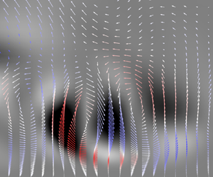
Investigation and decomposition of the SFS shear stress revealed that the filtered momentum transport deficit can be primarily attributed to convective residual velocity motions, whose structures are analysed herein. Fluctuation data of  $u$,
$u$,  $T$ and $\rho$ are extracted in several planes. In addition, the second-order residual velocity term $-\bar {\rho } u^{\prime \prime } v^{\prime \prime }$ is also extracted for filter width $\bar {\varDelta }_{x,z}^{(3)}$ (see table 4) and shown in wall-parallel planes in figures 10–12 for the M8 case. Figure 10 shows contours at $y^*=10$, which is at the location of the first peak of the SFS shear stress; figure 11 depicts contours at $y^*=28$, which corresponds to the valley location; figure 12 illustrates data at $y^*=60$, which is at the location of the second peak.

Figure 10. Instantaneous snapshot in the  $y^*=10$ ( $\kern 1.5pt y/\delta = 0.035$) wall-parallel plane for M8. Statistical fluctuation of (a) streamwise velocity, (b) temperature, (c) density and (d) second-order residual velocity contribution $-\bar {\rho } u^{\prime \prime } v^{\prime \prime }$ to the shear SFS stress for the filter width $\bar {\varDelta }_{x,z}^{(3)}$. (a,b) statistical Favre fluctuation, (c) statistical Reynolds fluctuation and (d) residual shear stress.

Figure 11. Instantaneous snapshot in the  $y^*=28$ ( $y/\delta = 0.11$) wall-parallel plane for M8. Statistical fluctuation of (a) streamwise velocity, (b) temperature, (c) density and (d) second-order residual velocity contribution $-\bar {\rho } u^{\prime \prime } v^{\prime \prime }$ to the SFS shear stress for the filter width $\bar {\varDelta }_{x,z}^{(3)}$. (a,b) statistical Favre fluctuation, (c) statistical Reynolds fluctuation and (d) residual shear stress.

Figure 12. Instantaneous snapshot in the  $y^*=60$ ( $\kern 1.5pt y/\delta = 0.28$) wall-parallel plane for M8. Statistical fluctuation of (a) streamwise velocity, (b) temperature, (c) density and (d) second-order residual velocity contribution $-\bar {\rho } u^{\prime \prime } v^{\prime \prime }$ to the SFS shear stress for the filter width $\bar {\varDelta }_{x,z}^{(3)}$. (a,b) statistical Favre fluctuation, (c) statistical Reynolds fluctuation and (d) residual shear stress.
The  $u$ fluctuation field at $y^*=10$ shown in figure 10 exhibits the typical streaky structures. The low-speed streaks are accompanied by the upward ( $v\textrm{''}>0$) vertical transport of the near-wall fluid, known as ejection events. The high-speed streaks are accompanied by the downward ( $v\textrm{''}<0$) vertical transport of higher-speed fluid, known as sweep events. Similar streaky structures were reported in many DNS studies of compressible wall-bounded flows (Duan et al. Reference Duan, Beekman and Martin2010, Reference Duan, Beekman and Martin2011; Pirozzoli & Bernardini Reference Pirozzoli and Bernardini2011; Kawai Reference Kawai2019; Xu et al. Reference Xu, Wang, Wan, Yu, Li and Chen2021a). The spanwise spacing of the high-speed streaks is visibly wider than that of the low-speed streaks. The $T$ and $\rho$ fluctuation fields at $y^*=10$ show similar streaky structures, and the comparison with the $u$ field clearly shows that low-temperature/high-density and high-temperature/low-density streaks correlate closely with low-speed and high-speed streaks, respectively. In addition, the $T$ fluctuation pattern is quite similar to the $u$ one. Such similarity near the wall was observed in supersonic boundary layers (Pirozzoli & Bernardini Reference Pirozzoli and Bernardini2011) and boundary layers with a temperature gradient (Toki & Bellan Reference Toki and Bellan2021, Reference Toki and Bellan2022). This indicates that structural similarity between velocity and temperature holds even at hypersonic conditions. In contrast, the $-\bar {\rho } u^{\prime \prime } v^{\prime \prime }$ field does not exhibit clear streaky structures because it is driven by the residual velocities, hence, small in scale, resulting in highly localized structures. In addition, its value is on average positive indicating filtered momentum transport in the mean statistical direction.
The  $u$ fluctuation field at $y^*=28$ shown in figure 11 also exhibits streaky structures. The similarity between the $u$ and $T$ still holds. However, careful observation of the $T$ fluctuation contour reveals that negative values are more extreme than positive ones. Similarly, the positive $\rho$ fluctuations are more extreme than the negative ones. The skewness in the $T$ fluctuations is driven by the mean temperature profile. As shown in figure 2, the mean temperature profile can be split around $y/\delta = 0.1$ to two layers: lower layer with strong temperature variation near the wall, and upper layer with mild variation toward the centre of the channel. The plane at $y^*=28$ ( $\kern 1.5pt y/\delta = 0.11$) is close to the interface of these layers, and therefore, the ejected fluid is accompanied by strong temperature fluctuations, whereas the swept one by mild fluctuations. The contribution of the $-\bar {\rho } u^{\prime \prime } v^{\prime \prime }$ field at $y^*=28$ also shows patchy structures, but its value becomes more distributed than $y^*=10$. Interestingly, the negative contribution to the SFS shear stress is observable in this plane, indicating that the residual velocity locally acts to reduce the average SFS shear stress. Such negative contribution is hardly observed at $y^*=10$.
The  $u$ fluctuation field at $y^*=60$ in figure 12 shows that the spanwise spacing of the velocity streaks are wider than that at $y^*=10$ and $28$. The similarity between the $u$ and $T$ becomes less clear. The $-\bar {\rho } u^{\prime \prime } v^{\prime \prime }$ field at $y^*=60$ depicts similar negative patchy structures to that at $y^*=28$. This result implies that the negative contribution to momentum transport in the SFS scale is observable at any $y$ locations over $y^*=28$. Therefore, to elucidate the cause of the SFS shear stress deficit, the reason why the negative contributions are enhanced around $y^*=28$ should be explored.
To investigate flow dynamics in the wall-normal direction, figure 13 shows contours of  $u$ fluctuation, $T$,
$T$,  $\rho$ and $-\bar {\rho } u^{\prime \prime } v^{\prime \prime }$ for the filter width $\bar {\varDelta }_{x,z}^{(3)}$ in cross-stream planes for all Mach numbers. Since the $-\bar {\rho } u^{\prime \prime } v^{\prime \prime }$ field has small-scale features and it is highly localized, a few selected regions where the strong negative contribution is observed are extracted. The $u$ fluctuation contour shows a cross-section of low-speed and high-speed streaks in the dash-dotted line square box. The cross-section reveals that the spanwise spacing of the low-speed streaks increases away from the wall for $y/\delta < 0.15$ in all Mach number cases. Such volumetric expansion may be explained as follows. The low-speed streak is accompanied by low-temperature/high-density fluid, while the high-speed streak is accompanied by high-temperature/low-density fluid. At the interface between these streaks, heat transfer is established from the high-temperature fluid of the high-speed streak to the low-temperature fluid of the low-speed streak. Therefore, the fluid of the low-speed streak expands around such an interface, and the volumetric expansion induces variation in spanwise spacing of the low-speed streak. This explanation is consistent with $T$ and $\rho$ contours in this plane. The low-speed streak in the dash-dotted line square box extends to $y/\delta =0.25$, whereas the temperature in the streak largely increases from the wall in all cases. Following the temperature variation, the density decreases in the streak. These $T$ and $\rho$ contours indicate that volumetric expansion occurs in the streak.

Figure 13. Instantaneous snapshot in cross-stream planes for M6, M7 and M8: (a–c) streamwise velocity fluctuations, (d–f) temperature, (g–i) density and (j–l) second-order residual velocity contribution  $-\bar {\rho } u^{\prime \prime } v^{\prime \prime }$ to the SFS shear stress with the filter width $\bar {\varDelta }_{x,z}^{(3)}$. Results are shown for (a,d,g,j) M6, (b,e,h,k) M7 and (c,f,i,l) M8.
As the result of the expansion of the low-speed streak, the high-speed streak is entrained under the low-speed streak, as shown in the region surrounded by the dashed line. The  $-\bar {\rho } u^{\prime \prime } v^{\prime \prime }$ field shows a strong negative value in this very region. In addition, the strong negative $-\bar {\rho } u^{\prime \prime } v^{\prime \prime }$ is observable only below $y/\delta \approx 0.2$, which corresponds to $y^* \approx 45$. This result indicates that the negative contribution is enhanced below this location, although the wall-parallel planes at $y^*=28$ and $y^*=60$ (figures 11d and 12d) depicted similar $-\bar {\rho } u^{\prime \prime } v^{\prime \prime }$ structures. Thus, flow dynamics around the interface between the high-speed and low-speed streaks is the key for understanding of the SFS shear stress deficit.
To elucidate the flow dynamics in the region surrounded by the smaller dashed box in figure 13, figure 14 illustrates vectors of fluctuation velocities and residual ones on the  $-\bar {\rho } u^{\prime \prime } v^{\prime \prime }$ contour in the cross-stream plane for the M8 case. Figure 14(a) shows fluctuation velocity vectors $(v\textrm{''}, w\textrm{''}$) coloured by $u\textrm{''}$ values, and figure 14(b) provides residual velocity vectors $(v^{\prime \prime }, w^{\prime \prime }$) coloured by $u^{\prime \prime }$ values. For the sake of description, the region surrounded by a black dashed line is called region 1, and the region surrounded by a white dashed line is called region 2. Strong negative $-\bar {\rho } u^{\prime \prime } v^{\prime \prime }$ are observed in these regions.

Figure 14. Vectors of (a) fluctuation velocities and (b) residual velocities obtained via a filter width  $\bar {\varDelta }_{x,z}^{(3)}$ in the cross-stream plane for M8 coloured by streamwise velocity fluctuations $u\textrm{''}$ and residual velocity $u^{\prime \prime }$, respectively. The $-\bar {\rho } u^{\prime \prime } v^{\prime \prime }$ contour is shown in the background with a greyscale colourmap.
The  $(v\textrm{''}, w\textrm{''}$) vectors show that red-coloured vectors are directed upward in region 1, indicating that higher-speed fluid moves upward. However, the mean streamwise velocity monotonically increases from the bottom wall, and thus, the higher-speed fluid should originate from the upper region. The counter-gradient motion can be explained as follows. As shown in figure 13, the high-speed streak is entrained under the low-speed streak due to the volumetric expansion of the low-speed streak. Since the low-speed streak is accompanied by the ejection event, partial fluid of the high-speed streak is rolled up by the ejection around the interface between the streaks. The rolling up induces the counter-gradient motion of the higher-speed fluid. By contrast, partial fluid of the low-speed streak is drawn into the high-speed fluid in region 2, and the relatively low-speed fluid is directed downward. Since these motions act to accelerate the upper fluid and decelerate the lower fluid, contributions of them are against the mean statistical direction of momentum transport.
Scales of these motions should be smaller than those of streaky structures because they occur only around the interface between the streaks. Therefore, these motions can be removed by the spatial filter. The  $(v^{\prime \prime }, w^{\prime \prime }$) vectors in figure 14(b) clearly show the effect of the spatial filter on these motions because the vectors indicate velocity components removed by the spatial filter. The $(v^{\prime \prime }, w^{\prime \prime }$) vectors reveal that a higher-residual velocity fluid moves upward, and a lower-residual velocity fluid moves downward in regions 1 and 2, respectively. These motions, contributions of which are against the mean statistical direction of momentum transport, are removed by the spatial filter. Since the SFS shear stress is defined as acting to supplement contributions of the removed motions, the SFS shear stress should locally work against the mean statistical direction. Hence, the $(v^{\prime \prime }, w^{\prime \prime }$) vectors imply that the counter-gradient motions of the residual velocity induce the SFS shear stress deficit.
4.5. Quadrant analysis for residual velocity motions
A powerful method to investigate contributions of turbulent motions is a quadrant analysis. Details about a quadrant analysis may be found in Wallace (Reference Wallace2016). Generally, a quadrant analysis is applied to turbulent fluxes in mean flow fields. Quadrants for the Reynolds shear stress  $-\langle \rho \rangle \{ u\textrm{''} v\textrm{''} \}$ are classified in the following four categories: Q1 $(u\textrm{''}>0, v\textrm{''}>0)$, Q2 $(u\textrm{''}<0, v\textrm{''}>0)$, Q3 $(u\textrm{''}<0, v\textrm{''}<0)$ and Q4 $(u\textrm{''}>0, v\textrm{''}<0)$. The Q2 and Q4 motions correspond to ejection and sweep events. The Q1 and Q3 motions, which are counter-gradient-type motions, are called outward and inward interactions by Wallace, Eckelmann & Brodkey (Reference Wallace, Eckelmann and Brodkey1972). The upward motion of the higher-speed fluid in figure 14 corresponds to the Q1 motion, and the downward motion of the lower-speed fluid corresponds to the Q3 motion. In this section the quadrant analysis is also applied to the second-order residual velocity term $\langle -\bar {\rho } u^{\prime \prime } v^{\prime \prime } \rangle$ for the filter width $\bar {\varDelta } _{x,z}^{(3)}$ to discuss its contributions to the SFS shear stress. Similarly to the Reynolds shear stress $-\langle \rho \rangle \{ u\textrm{''} v\textrm{''}\}$, quadrants for the $\langle -\bar {\rho } u^{\prime \prime } v^{\prime \prime } \rangle$ are classified in the following four categories: Q1 $(u^{\prime \prime }>0, v^{\prime \prime }>0)$, Q2 $(u^{\prime \prime }<0, v^{\prime \prime }>0)$, Q3 $(u^{\prime \prime }<0, v^{\prime \prime }<0)$ and Q4 $(u^{\prime \prime }>0, v^{\prime \prime }<0)$.
The  $-\langle \bar {\rho } \rangle \{ u\textrm{''} v\textrm{''}\}$ and the $\langle -\bar {\rho } u^{\prime \prime } v^{\prime \prime } \rangle$ are decomposed to quadrant contributions and their profiles in the bottom wall side are shown in figures 15 and 16 for the M6, M7 and M8 cases. The $-\langle \rho \rangle \{ u\textrm{''} v\textrm{''} \}$ can be decomposed to
 \begin{equation} {-}\langle \rho \rangle \{ u\textrm{''} v\textrm{''}\} = \sum_{q=1}^{4}{-\langle \rho \rangle \{ u\textrm{''}v\textrm{''}\}_{q}}, \end{equation}
Figure 15. Quadrant contributions to Reynolds shear stress in the M6, M7 and M8 cases.

Figure 16. Quadrant contributions to SFS shear stress for the filter width  $\bar {\varDelta }_{x,z}^{(3)}$ in the M6, M7 and M8 cases.
where  $-\langle \rho \rangle \{ u\textrm{''} v\textrm{''} \}_{q}$ is the $q$th quadrant contribution. The first quadrant is computed as
 \begin{equation} \langle \rho \rangle \{
u\textrm{''} v\textrm{''} \}_{1}
=\frac{1}{N_{t}N_{x}N_{z}}\left( \sum_{\substack{l=1\\
u\textrm{''}>0,v\textrm{''}>0}}^{N_{t}} \sum_{\substack{k=1\\
u\textrm{''}>0,v\textrm{''}>0}}^{N_{z}} \sum_{\substack{i=1\\
u\textrm{''}>0,v\textrm{''}>0}}^{N_{x}}( \rho u\textrm{''} v\textrm{''})_{ikl}\right)\!.
\end{equation}
\begin{equation} \langle \rho \rangle \{
u\textrm{''} v\textrm{''} \}_{1}
=\frac{1}{N_{t}N_{x}N_{z}}\left( \sum_{\substack{l=1\\
u\textrm{''}>0,v\textrm{''}>0}}^{N_{t}} \sum_{\substack{k=1\\
u\textrm{''}>0,v\textrm{''}>0}}^{N_{z}} \sum_{\substack{i=1\\
u\textrm{''}>0,v\textrm{''}>0}}^{N_{x}}( \rho u\textrm{''} v\textrm{''})_{ikl}\right)\!.
\end{equation}
The other quadrants are computed in the same way based on each sign condition. The  $\langle -\bar {\rho } u^{\prime \prime } v^{\prime \prime } \rangle$ can be also decomposed as
 \begin{equation} {-}\langle \bar{\rho} u^{\prime \prime} v^{\prime \prime} \rangle = \sum_{q=1}^{4}{-\langle \bar{\rho} u^{\prime \prime} v^{\prime \prime} \rangle_{q}}, \end{equation}
where  $-\langle \bar {\rho } u^{\prime \prime } v^{\prime \prime } \rangle _{q}$ is the $q$th quadrant contribution computed based on the signs of the residual velocities $u^{\prime \prime }$ and $v^{\prime \prime }$.
Figure 15 shows that contributions of the Q2 and Q4 motions to the  $-\langle \bar {\rho } \rangle \{ u\textrm{''} v\textrm{''} \}$ are positive, and those of the Q1 and Q3 motions are negative in all cases. A comparison among the cases shows that there is a difference in the Q2 and Q3 motions below $y^*=10$, whereas contributions in all motions collapse for $y^*>10$, indicating that the Mach number hardly affects quadrant contributions to the Reynolds shear stress for $y^*>10$. Inspecting values of each motion, positive contributions of the Q2 and Q4 motions are found to be much larger than negative contributions of the Q1 and Q3 motions, indicating that the Q2 and Q4 motions are dominant in the Reynolds shear stress.
The contributions to the  $-\langle \bar {\rho } u^{\prime \prime } v^{\prime \prime } \rangle$ in figure 16 also show that contributions of the Q2 and Q4 motions are positive and those of the Q1 and Q3 motions are negative. However, their behaviours are much different from the $-\langle \bar {\rho } \rangle \{ u\textrm{''} v\textrm{''} \}$ for $y^*>10$. Contributions of the Q2 and Q4 motions have positive peaks around $y^*=30$, and those of the Q1 and Q3 motions have negative peaks at the same $y^*$ location. In addition, those peaks become more pronounced for higher Mach numbers. Especially, negative contributions of the Q1 and Q3 motions for the M8 case are over 1.5 in absolute value, and they are comparable with those of the Q2 and Q4 motions. This result indicates that the negative contributions of the Q1 and Q3 motions are also significant in small-scale turbulence, and can influence the SFS shear stress.
To further investigate impacts of the negative contributions, the sum of the Q1 and Q3 contributions and that of the Q2 and Q4 motions are compared. Figure 17 provides these ratios for the  $-\langle \bar {\rho } \rangle \{ u\textrm{''} v\textrm{''}\}$ and the $-\langle \bar {\rho } u^{\prime \prime } v^{\prime \prime } \rangle$ as a function of $y^*$. The ratio for the $-\langle \bar {\rho } \rangle \{u\textrm{''} v\textrm{''}\}$ shows agreement for $y^*>10$, and its value is below 0.3 in almost the entire domain, indicating that the negative contributions are smaller than 30 % of positive contributions. In contrast, the ratio for $-\langle \bar {\rho } u^{\prime \prime } v^{\prime \prime } \rangle$ is much larger, and it has a positive peak at $y^*=30$ in all cases. Especially, the peak in M8 reaches around 0.8, indicating that the negative contributions reach 80 % of positive contributions in the SFS scale turbulence. The negative contributions are attributed to the counter-gradient motions observed in § 4.4. Therefore, the positive peak at $y^*=30$ statistically proves that the counter-gradient motions, which induces the SFS shear stress deficit, are enhanced at this location.

Figure 17. Ratio of negative and positive quadrant contributions for (a) Reynolds shear stress and (b) SFS shear stress with the filter width  $\bar {\varDelta }_{x,z}^{(3)}$ in M6, M7 and M8. The subscript $(1+3)$ indicates the sum of the Q1 and Q3 contributions, and the subscript $(2+4)$ indicates the sum of the Q2 and Q4 contributions.
4.6. Effects of filter directions on SFS shear stress
Given the highly anisotropic nature of wall-bounded hypersonic turbulence, the choice of a specific filtering strategy is an important factor determining the values of the SFS shear stress. To investigate the effects of the ratio of filter widths in the  $x$ and $z$ directions, a sharp spectral filter is applied in only $x$ or $z$, representing the two aspect ratio extremes of a two-dimensional filter applied in the $(x, z)$ plane. The filter widths chosen for each direction are $\bar {\varDelta }_{x}^{(3)}$ and $\bar {\varDelta }_{z}^{(3)}$, and their combination into a two-dimensional filter is denoted as $\bar {\varDelta }_{x, z}^{(3)}$.
Figure 18 shows that the combination of the SFS stresses obtained from the one-directional filtering operations amounts to the total stresses extracted from the two-direction filter  $\bar {\varDelta }_{x, z}^{(3)}$. The SFS shear stress due to the under-resolved scales in the $z$ direction is significantly below $y^*\approx 20$, whereas those associated with the $x$ direction become dominant in the outer layer region. This result indicates that, from an LES perspective, flow structures near the wall are more likely to be under-resolved in the $z$ direction, while the grid resolution in $x$ becomes more critical away from the buffer layer, in the core of the flow. These observations are consistent with results shown in figures 10–12. Furthermore, the SFS stresses obtained via filtering in the $x$ exhibit a negative peak around $y^*=20$, indicating that the SFS shear stress deficit is driven by SFS activity in the streamwise direction. This analysis underscores the importance of accounting for flow anisotropy when developing SFS stresses for hypersonic flows.

Figure 18. The SFS shear stress extracted using filtering operations only in the streamwise or spanwise direction, compared with both filters combined. The  $\bar {\varDelta }_{x}^{(3)}$ and $\bar {\varDelta }_{z}^{(3)}$ are the filter widths of one-directional filters in the $x$ and $z$ direction, respectively. Black circles represent the data obtained from two-directional filters $\bar {\varDelta }_{x,z}^{(3)}$. Profiles are shown as a function of (a) $y/\delta$ and (b) $y^*$. Profiles of $y^*$ are only shown for the bottom wall side.
4.7. Effects of Reynolds number on SFS shear stress
Analyses for the M6, M7 and M8 cases revealed that the second-order residual velocity term induces the SFS shear stress deficit at hypersonic conditions. Since the deficit is attributed to small-scale turbulence as shown in § 4.4, the SFS shear stress can depend on Reynolds number. To investigate effects of Reynolds number on the SFS shear stress, figure 19 compares averaged SFS shear stress profiles among the higher-Reynolds-number cases: M8-H1, M8-R1 and M8-R2. For the purpose of comparison, data for the M8 case is also included. Similarly to § 4.2, the same three combinations of filter widths are tested:  $\bar {\varDelta }_{x,z}^{(1)}$, $\bar {\varDelta }_{x,z}^{(2)}$ and $\bar {\varDelta }_{x,z}^{(3)}$. These filter widths are decided as a function of $\delta$, not the grid spacing. Therefore, the ratio of the filter width and grid spacing is not the same between the cases. For example, $\bar {\varDelta }_{x,z}^{(1)}$ is twice as large as grid spacing for M8, three times for M8-H1 and M8-R1, and four times for M8-R2. Additionally, figure 20 shows contours of streamwise velocity fluctuations of filtered fields for the three filter widths in the wall-parallel plane at $y^*=26$ for the M8-R2 case to discuss the effect of filter widths on flow structures. Data of the unfiltered flow field are also included in the figure.

Figure 19. Exact SFS shear stress profiles as a function of (a,c,e)  $y/\delta$ and (b,d,f) $y^*$ for higher-Reynolds-number cases. Profiles as a function of $y^*$ are only shown in the bottom wall side. The filter widths are (a,b) $\bar {\varDelta }_{x,z}^{(1)}$, (c,d) $\bar {\varDelta }_{x,z}^{(2)}$ and (e,f) $\bar {\varDelta }_{x,z}^{(3)}$.

Figure 20. Instantaneous snapshot of streamwise velocity fluctuations in spatial filtered fields in the  $y^*=26$ ( $\kern 1.5pt y/\delta = 0.03$) wall-parallel plane for M8-R2: (a) unfiltered, (b) $\bar {\varDelta }_{x,z}^{(1)}$, (c) $\bar {\varDelta }_{x,z}^{(2)}$ and (d) $\bar {\varDelta }_{x,z}^{(3)}$. (a) statistical Favre fluctuation velocity, and (b–d) statistical Favre fluctuation of Favre filtered velocity.
The SFS shear stress with  $\bar {\varDelta }_{x,z}^{(1)}$ is almost null in M8, but those in the other cases are substantial. The profiles in M8-H1 and M8-R1 have a negative peak around $y^*=25$, and they are similar to that in M8 with $\bar {\varDelta }_{x,z}^{(2)}$ (figure 7). The profile in M8-R2 has a deficit near $y^*=25$ and it is analogous to that in M8 with $\bar {\varDelta }_{x,z}^{(3)}$. The comparison with figure 7 reveals that the $y/\delta$ locations of the negative peak and the deficit in the higher-Reynolds-number cases are closer to the wall than those for the M8 case, however, the $y^*$ locations of them are the same. This result indicates that the negative peak and the deficit of the SFS shear stress can appear in the buffer region even at high Reynolds number. In addition, the SFS shear stress for the M8-H1 and M8-R1 cases exhibits excellent collapses with all filter widths. These two cases have different channel widths, but Mach numbers and Reynolds numbers are almost the same. Therefore, the collapses imply that the SFS shear stress can be scaled under the same Reynolds number and Mach number condition.
The SFS shear stress with  $\bar {\varDelta }_{x,z}^{(2)}$ in M8-H1 and M8-R1 has a deficit around $y^*=25$, while that in M8-R2 does not have a deficit. The peak in M8-R2 is over 0.25 and quite larger than the other cases. Generally, flow structures become finer with increasing Reynolds number. The comparison of velocity fluctuation fields around $y^*=25$ between M8 and M8-R2 (figures 11a and 20a) shows that M8-R2 has much finer structures. Therefore, even when the same spatial filter is applied, the effect of the filter on M8-R2 is more significant. Accordingly, the SFS shear stress becomes larger with an increase in Reynolds number. The absence of the deficit in M8-R2 is attributed to its fine flow structures. Momentum transport in the mean statistical direction is induced by large-scale motions comparable with velocity streaks. On the other hand, the counter-gradient momentum transport of the second-order residual velocity term occurs only in the smaller scale as shown in § 4.4. Therefore, when a strong spatial filter is applied, the momentum transport in the mean statistical direction overwhelms the counter-gradient one.
The SFS stress with  $\bar {\varDelta }_{x,z}^{(3)}$ in M8-H1 and M8-R1 does not have a deficit as well as M8-R2, because of the strong spatial filter. The peak in M8-R2 reaches 0.6 indicating that the SFS shear stress is comparable to the wall shear stress and Reynolds shear stress. Theoretically, the SFS shear stress value becomes closer to the Reynolds shear stress with an increase in the filter width, because an infinite filter width corresponds to averaging in homogeneous directions. Therefore, the quite large SFS shear stress in M8-R2 implies that the spatial filter affects the largest-scale structures in the flow field.
The comparison of the SFS shear stress among different filter widths revealed that the deficit of the SFS shear stress is observable in the buffer region at any Reynolds number with certain filter widths, while the deficit disappears when a stronger spatial filter is applied. It may be expected that the SFS shear stress deficit does not need to be considered in LES modelling of hypersonic wall-bounded flows with a strong spatial filter. However, the streamwise velocity fluctuations in filtered fields shown in figure 20 indicate that the strong spatial filter induces inevitable problems. The contour with  $\bar {\varDelta }_{x,z}^{(1)}$ shows a similar velocity field to that of an unfiltered one. The similarity implies that important turbulent motions can be resolved with $\bar {\varDelta }_{x,z}^{(1)}$. On the other hand, the contours with $\bar {\varDelta }_{x,z}^{(2)}$ and $\bar {\varDelta }_{x,z}^{(3)}$ show that some structures observed in the unfiltered field disappear in the spatial filtered ones. For example, the box with a solid black line contains several low- and high-speed streaks in the unfiltered field, whereas they are not observed in the contour with $\bar {\varDelta }_{x,z}^{(3)}$, indicating that there is an upper limit of the spatial filter width to resolve important large-scale structures.
To further investigate effects of the spatial filter width on flow fields, figure 21 provides streamwise and spanwise spectra of the Reynolds shear stress at  $y^*=25$ for the M8, M8-H1, M8-R1 and M8-R2 cases. The $k_x$ and $k_z$ indicate wavenumbers within the computational domain in the streamwise and spanwise directions, respectively. The cutoff wavenumbers of the applied spatial filters are provided by red, green and blue solid lines. The spectra are almost constant for low wavenumbers, and start to decrease at a certain wavenumber, indicating that the energy cascade occurs in all cases. The comparison among the cases reveals that the wavenumber where the energy cascade starts, increases with an increase in Reynolds number. For example, the energy cascade in the spanwise direction occurs for $k_z > 10$ in M8, whereas that occurs for $k_z > 60$ in M8-R2. Most SFS models are built based on the energy cascade, thus, these wavenumbers correspond to the upper limit of the spatial filter width for SFS models. The blue line indicates the filter for $\bar {\varDelta }_{x,z}^{(1)}$, and the energy cascade in the spanwise direction in M8-R2 starts around this line. Therefore, the upper limit of the spatial filter width for M8-R2 is close to $\bar {\varDelta }_{x,z}^{(1)}$. Similarly, the spectra indicate that the upper limit for M8-H1 and M8-R1 is located around $\bar {\varDelta }_{x,z}^{(2)}$ and, for M8, is around $\bar {\varDelta }_{x,z}^{(3)}$. All of these filter widths around the upper limits are approximately four to eight times as large as DNS grid spacings for each case. Therefore, compared with the current DNS resolution, it is expected that resolutions of $\Delta x^* \approx 40 \sim 80$ and $\Delta z^* \approx 15 \sim 30$ are required for well-resolved LES. In addition, figure 19 shows that the SFS stresses with these upper limit filters have the SFS shear stress deficit in all cases. Hence, LES modelling for hypersonic wall-bounded flows needs to account for the deficit of the SFS shear stress so that important large-scale turbulence is resolved.

Figure 21. One-dimensional spectra of  $\rho u\textrm{''} v\textrm{''}$ at $y^*=25$ in (a) the streamwise direction and (b) the spanwise direction for higher-Reynolds-number cases. The blue, green and red solid lines indicate cutoff wavenumbers for $\bar {\varDelta }_{x,z}^{(1)}$, $\bar {\varDelta }_{x,z}^{(2)}$ and $\bar {\varDelta }_{x,z}^{(3)}$, respectively.
5. Conclusion
Direct numerical simulations of hypersonic turbulent Couette flows have been performed to investigate exact SFS shear stress in wall-bounded turbulent flows at hypersonic conditions. The simulations encompass three lower-Reynolds-number cases with different Mach numbers and higher-Reynolds-number cases. The Mach number of the top wall is 6, 7 or 8 in the lower-Reynolds-number cases and in the higher-Reynolds-number cases is 8. The friction Reynolds number in the lower-Reynolds-number cases ranges from 621 to 713 and it increases with an increase in Mach number, whereas the semi-local friction Reynolds number ranges from 213 to 277 and it decreases with an increase in Mach number. The friction Reynolds number in the higher-Reynolds-number cases ranges from 1278 to 2355 and the semi-local friction Reynolds number ranges from 384 to 698.
The mean profiles showed that the mean temperature and density largely vary in the wall-normal direction, however, the Trettel & Larsson (Reference Trettel and Larsson2016)'s transformation works well for the mean streamwise velocity profiles. In addition, there are good agreements of semi-local scaled velocity fluctuation correlations between all cases. The analysis of mean profiles and turbulent fluctuations revealed that compressibility effects on mean flow fields are so moderate that the existing scaling law holds under the present hypersonic conditions. On the other hand, analyses of SFS shear stress for the lower-Reynolds-number cases revealed that the averaged SFS shear stress with a weaker filter works against the mean statistical direction of momentum transport. The averaged SFS shear stress with a stronger filter works in the mean statistical direction, however, it has two peaks separated by the SFS shear stress deficit. The deficit becomes more pronounced for higher Mach numbers, and such deficit of the SFS shear stress was not observed in the low-speed regime. Thus, the deficit can be attributed to compressibility effects, and LES modelling needs to account for compressibility effects even at conditions where compressibility effects on mean flow fields are moderate.
Through the mathematical transformation, the SFS shear stress was decomposed to transport of the resolved flow, contributions of the second-order term in the residual velocity and the third-order correlations of residual components. The comparison among these terms clarified that contributions of the second-order term in residual velocity motions is dominant, indicating that the SFS shear stress mainly originates from the second-order residual velocity term. Thus, flow dynamics in the SFS shear stress deficit should be explained by investigation of the residual velocity motions.
Visualization of flow structures in the wall-parallel planes revealed that the spanwise spacing of the high-velocity streaks are visibly wider than the low-velocity streaks. The temperature field is quite similar to the velocity field in the vicinity of the wall, however, the similarity becomes less clear away from the wall. The visualized contribution of the second-order residual velocity term is highly localized, and its strong negative value is observable at the location of the SFS shear stress deficit. The velocity fluctuation field in the cross-stream plane showed that the spanwise spacing of the low-speed streak increases in the wall-normal direction due to the volumetric expansion. As a result, the high-speed streak is entrained under the low-speed streak. The contour of the contribution of the second-order term in residual velocity displays its strong negative value around the interface between the low- and high-speed streaks. This result implies that flow dynamics around such an interface is the key for understanding of the SFS shear stress deficit. Vectors of fluctuation velocities and residual velocities were shown to examine flow dynamics in the negative contribution region. The vectors of fluctuation velocities revealed that partial fluid of the high-speed streak is rolled up by a close ejection event due to the volumetric expansion of the low-speed streak. In contrast, partial fluid of the low-speed streak is drawn into the higher-speed fluid, and the relatively low-speed fluid is directed downward. Since these motions act to accelerate the upper fluid and decelerate the lower fluid, contributions of these motions are against the mean statistical direction of momentum transport. The vectors of the residual velocities clarified that these counter-gradient motions are removed by the spatial filter. Since the SFS shear stress is defined as acting to supplement contributions of the removed motions, the SFS shear stress locally works against the mean statistical direction of momentum transport in the region and induces the SFS shear stress deficit.
A quadrant analysis for the residual velocities statistically supported the discussion based on the visualization of the flow field. Quadrants of the counter-gradient motions for the residual velocities have a negative peak, and their negative contributions become more pronounced for a higher Mach number. Since the negative contributions correspond to the counter-gradient momentum transport, the quadrant analysis statistically proved that the negative contributions are locally enhanced, and the SFS shear stress deficit is induced by the counter-gradient motions.
The SFS stress analysis carried out with one-directional filters revealed that the SFS shear stress deficit is associated with gradients in the streamwise direction, and it is a highly directional phenomenon. Therefore, it is recommended that the highly anisotropic state of wall-bounded hypersonic turbulence is taken into account in the development of SFS models.
The SFS shear stress deficit is also observable in the buffer region at any Reynolds number with a certain filter width. On the other hand, the deficit disappears when a strong spatial filter is applied. However, observation of the filtered velocity fluctuation field revealed that such a strong spatial filter can remove velocity streaks, indicating that LES with the strong filter cannot resolve important large-scale structures. In addition, energy spectra of the Reynolds shear stress clarified the upper limit of the spatial filter width for SFS models. When the upper limit spatial filter is applied, the SFS shear stress deficit is still observable in all cases. Hence, LES modelling for hypersonic wall-bounded flows needs to account for the SFS shear stress deficit to achieve reasonable resolution.
This study focuses only on the SFS shear stress, however, there are other components of the total SFS stress tensor, as well as SFS heat fluxes and kinetic energy transport and SFS turbulent heat dissipation that need to be closed. The analyses of these other SFS terms will be carried out in future work.
Acknowledgements
The authors acknowledge the computational support of the Rosen Center for Advanced Computing (RCAC) at Purdue.
Funding
The authors acknowledge support through ONR grant nos. N00014-20-1-2662 (ONR-YIP, PI: Scalo), N00014-21-1-2475 (ONR-MURI, PI: Venkat Raman) and N00014-23-1-2560 (Core ONR program, PI: Carlo Scalo) with Dr. Eric Marineau as program manager. This work used Purdue Anvil CPU at Purdue through allocation MCH220031 from the Advanced Cyberinfrastructure Coordination Ecosystem: Services & Support (ACCESS) program, which is supported by National Science Foundation grant nos. 2138259, 2138286, 2138307, 2137603 and 2138296 (Boerner et al. Reference Boerner, Deems, Furlani, Knuth and Towns2023).
Declaration of interests
The authors report no conflict of interest.
Appendix A. Grid refinement study and domain size
As shown in table 2, three different grids are used in the present DNS because of the wide range of Reynolds numbers. The grid-refinement studies of the three grids are performed for M8, M8-R1 and M8-R2. Figures 22–24 show transformed velocity profiles via Trettel & Larsson (Reference Trettel and Larsson2016)'s transformation and velocity fluctuation correlations. These figures clearly show grid convergence processes, and sufficiently converged profiles have excellent collapses among the different cases as shown in figures 3 and 4. In addition, to investigate the resolution requirements of the highest Mach number considered in this study, a grid sensitivity analysis of energy spectra and the SFS shear stress are conducted for M8, which is the case exhibiting the strongest SFS deficit. Figure 25 shows the streamwise velocity energy spectra in the streamwise direction and spanwise velocity spectra in the spanwise direction at  $y^*=28$, and figure 26 shows the SFS shear stress with $\bar {\varDelta }_{x,z}^{(3)}$. The energy spectra with the medium and fine grids collapse below $k_x=100$ and $k_z=50$. These wavenumbers are comparable with the cutoff wavenumbers of the weakest filter adopted, $\bar {\varDelta }_{x,z}^{(1)}$. The SFS shear stress with $\bar {\varDelta }_{x,z}^{(1)}$ shown in figure 7 revealed that its contribution is negligible, and thus, the spectra implies that the high-wavenumber turbulence is sufficiently well resolved to allow for the accurate extraction of SFS shear stresses. Moreover, the SFS shear stress with $\bar {\varDelta }_{x,z}^{(3)}$ in figure 26 shows acceptable collapse between medium and fine grids.

Figure 22. Grid sensitivity study for M8. (a) Transformed velocity profiles via Trettel & Larsson (Reference Trettel and Larsson2016)'s transformation and (b) velocity fluctuation correlations. Coarse,  $N_x \times N_y \times N_z = 384 \times 128 \times 192$; medium, $N_x \times N_y \times N_z = 512 \times 192 \times 256$; fine, $N_x \times N_y \times N_z = 768 \times 256 \times 384$.

Figure 23. Grid sensitivity study for M8-R1. (a) Transformed velocity profiles via Trettel & Larsson (Reference Trettel and Larsson2016)'s transformation and (b) velocity fluctuation correlations. Coarse,  $N_x \times N_y \times N_z = 256 \times 160 \times 128$; medium, $N_x \times N_y \times N_z = 512 \times 192 \times 256$; fine, $N_x \times N_y \times N_z = 768 \times 220 \times 384$.

Figure 24. Grid sensitivity study for M8-R2. (a) Transformed velocity profiles via Trettel & Larsson (Reference Trettel and Larsson2016)'s transformation and (b) velocity fluctuation correlations. Coarse,  $N_x \times N_y \times N_z = 256 \times 160 \times 128$; medium, $N_x \times N_y \times N_z = 512 \times 192 \times 256$; fine, $N_x \times N_y \times N_z = 768 \times 220 \times 384$; finer, $N_x \times N_y \times N_z = 1024 \times 256 \times 512$.

Figure 25. Grid sensitivity study of energy spectra at  $y^*=28$ for M8. (a) Streamwise velocity in the streamwise direction and (b) spanwise velocity in the spanwise direction. The blue, green and red solid lines indicate cutoff wavenumbers for $\bar {\varDelta }_{x,z}^{(1)}$, $\bar {\varDelta }_{x,z}^{(2)}$ and $\bar {\varDelta }_{x,z}^{(3)}$, respectively. Coarse, $N_x \times N_y \times N_z = 384 \times 128 \times 192$; medium, $N_x \times N_y \times N_z = 512 \times 192 \times 256$; fine, $N_x \times N_y \times N_z = 768 \times 256 \times 384$.

Figure 26. Grid sensitivity study of SFS shear stress with  $\bar {\varDelta }_{x,z}^{(3)}$ for M8 as a function of (a) $y/\delta$ and (b) $y^*$. Coarse, $N_x \times N_y \times N_z = 384 \times 128 \times 192$; medium, $N_x \times N_y \times N_z = 512 \times 192 \times 256$; fine, $N_x \times N_y \times N_z = 768 \times 256 \times 384$.
Figure 27 depicts two-point correlations of velocity fluctuations in homogeneous directions at  $y^*=10$ for the M8, M8-R1 and M8-R2 cases. The streamwise and spanwise correlations of velocity fluctuations all drop to almost zero, indicating that the present computational domain is sufficiently large. In addition, the correlation distance in a higher-Reynolds-number case becomes shorter. This result indicates that the largest scale of turbulence decreases with an increase in Reynolds number.

Figure 27. Two-point correlations of velocity fluctuations in (a,c,e) streamwise and (b,d,f) spanwise directions at  $y^*=10$ in M8, M8-R1 and M8-R2. (a,b) streamwise velocity, (c,d) wall-normal velocity and (e,f) spanwise velocity.
Appendix B. Filtered Navier–Stokes equations for the present coordinates
Practical LES should follow the compressible LES methodology in generalized curvilinear coordinates (Nagarajan, Lele & Ferziger Reference Nagarajan, Lele and Ferziger2007). Here, we consider a structured grid in the physical space  $\boldsymbol {y}$ to be transformed to computational space $\boldsymbol {x}$ in the present configuration:
 $$\begin{gather} x^i = x^i(y_1,y_2, y_3), \end{gather}$$
 $$\begin{gather}y_i = y_i(x^1,x^2, x^3), \end{gather}$$
where  $x^i$ and $y_i$ are the $i$th coordinate of each respective system of reference. The compressible filtered Navier–Stokes equations for generalized curvilinear coordinates are
 $$\begin{gather} \frac{\partial \overline{J \rho}}{\partial t} + \frac{\partial }{\partial x^j}( \overline{J \rho} \tilde v^j)= 0, \end{gather}$$
 $$\begin{gather}\frac{\partial \overline{J \rho}\tilde v^i}{\partial t} + \frac{\partial}{\partial x^j}(\overline{J \rho} \tilde v^i \tilde v^j + \overline{J p} g^{ij} - J \tilde \sigma^{ij} + \overline{J \rho} \tau^{ij})=-\varGamma^i_{qj}(\overline{J \rho} \tilde v^q \tilde v^j + \overline{J p} g^{qj} - J \tilde \sigma^{qj} + \overline{J \rho} \tau^{qj}), \end{gather}$$
 $$\begin{gather}\frac{\partial \overline{J E}}{\partial t} + \frac{\partial}{\partial x^j}(\overline{J(E + p)}\tilde v^j + J \tilde Q^{j})= \frac{\partial}{\partial x^k}( J \tilde \sigma^{ij}g_{ik}\tilde v^k )- \frac{\partial \overline{J \rho} C_p q^{j} }{\partial x^j}, \end{gather}$$
where  $J$ is the Jacobian of the transformation that is the determinant of the Jacobi matrix ( $J_{ij} = \partial y_i/\partial x^j$). The transformation between $u_i$ and $v^i$ is given by
 \begin{equation} v^j = u_i \frac{\partial x^j}{\partial y_i}. \end{equation}
The sub-filter terms are defined as
 $$\begin{gather} \tau^{ij} = \tilde{v^i v^j} - \tilde v^i \tilde v^j, \end{gather}$$
 $$\begin{gather}q^{j} = \tilde{T v^j} - \tilde T \tilde v^j. \end{gather}$$
In (B3)–(B5),  $g_{ij}$ and $g^{ij}$ are the covariant and contravariant metric tensors, respectively, and $\varGamma ^i_{qj}$ is the Christoffel symbol of the second kind. They are defined as
 $$\begin{gather} g_{ij} = \frac{\partial y_i \partial y_j}{\partial x^k \partial x^k}, \end{gather}$$
 $$\begin{gather}g^{ij} = \frac{\partial x^k \partial x^k}{\partial y_i \partial y_j}, \end{gather}$$
 $$\begin{gather}\varGamma^i_{qj} = \frac{\partial x^i}{\partial y_l} \frac{\partial^2 y_l}{\partial x^q \partial x^j}. \end{gather}$$
In the curvilinear frame of reference the total energy, the viscous stress tensor and the heat flux vector are described by slightly modified relations described below:
 $$\begin{gather} \frac{\overline{J p}}{\gamma - 1} = \overline{J E} - \frac{1}{2} \overline{J \rho} g_{ij} \tilde v^i \tilde v^j - \frac{1}{2} \overline{J \rho} g_{ij} \tau^{ij}, \end{gather}$$
 $$\begin{gather}\tilde \sigma^{ij} = \mu \left(g^{jk} \frac{\partial \tilde v^i}{\partial x^k} + g^{ik} \frac{\partial \tilde v^j}{\partial x^k} - \frac{2}{3} g^{ij}\frac{\partial \tilde v^k}{\partial x^k} \right)\!, \end{gather}$$
 $$\begin{gather}\tilde Q^j =-k g^{ij} \frac{\partial \tilde T}{\partial x^i}. \end{gather}$$
The present simulations are given by an orthogonal grid, and the grid spacing in streamwise and spanwise directions are uniform. Thus, the Jacobian and the velocities in computational space can be rewritten as
 $$\begin{gather} J = \frac{\partial y_1}{\partial x^1} \frac{\partial y_2}{\partial x^2} \frac{\partial y_3}{\partial x^3} = \frac{\partial y_2}{\partial x^2} = J_{22}, \end{gather}$$
 $$\begin{gather}v^1 = u_1, \quad v^2 = u_2/J_{22} \quad \text{and} \quad v^3 = u_3. \end{gather}$$
Substituting these velocities to the sub-filter terms in (B7) and (B8), one obtains
 $$\begin{gather} \begin{bmatrix} \tau^{11} & \tau^{12} & \tau^{13} \\ \tau^{21} & \tau^{22} & \tau^{23} \\ \tau^{31} & \tau^{32} & \tau^{33} \end{bmatrix}=\begin{bmatrix} \tau_{11} & \tau_{12}/J_{22} & \tau_{13} \\ \tau_{21}/J_{22} & \tau_{22}/(J_{22})^2 & \tau_{23}/J_{22} \\ \tau_{31} & \tau_{32}/J_{22} & \tau_{33} \end{bmatrix} \end{gather}$$
 $$\begin{gather}\begin{bmatrix} \sigma^{11} & \sigma^{12} & \sigma^{13} \\ \sigma^{21} & \sigma^{22} & \sigma^{23} \\ \sigma^{31} & \sigma^{32} & \sigma^{33} \end{bmatrix}=\begin{bmatrix} \sigma_{11} & \sigma_{12}/J_{22} & \sigma_{13} \\ \sigma_{21}/J_{22} & \sigma_{22}/(J_{22})^2 & \sigma_{23}/J_{22} \\ \sigma_{31} & \sigma_{32}/J_{22} & \sigma_{33} \end{bmatrix} \end{gather}$$
 $$\begin{gather}\begin{bmatrix} q^1 \\ q^2 \\ q^3 \end{bmatrix}=\begin{bmatrix} q_1 \\ q_2/J_{22} \\ q_3 \end{bmatrix}. \end{gather}$$
In addition, the contravariant metric tensors are rewritten as
 \begin{equation} \begin{bmatrix} g^{11} & g^{12} & g^{13} \\ g^{21} & g^{22} & g^{23} \\ g^{31} & g^{32} & g^{33} \end{bmatrix}=\begin{bmatrix} 1 & 0 & 0\\ 0 & 1/(J_{22})^2 & 0\\ 0 & 0 & 0 \end{bmatrix}. \end{equation}
The Christoffel symbols of the second kind are rewritten as
 $$\begin{gather} \varGamma^1_{qj} = \frac{\partial x^1}{\partial y_1} \frac{\partial^2 y_1}{\partial x^1 \partial x^1} = 0, \end{gather}$$
 $$\begin{gather}\varGamma^2_{qj} = \frac{\partial x^2}{\partial y_2} \frac{\partial^2 y_2}{\partial x^2 \partial x^2} = (\varGamma^2_{22}), \end{gather}$$
 $$\begin{gather}\varGamma^3_{qj} = \frac{\partial x^3}{\partial y_3} \frac{\partial^2 y_3}{\partial x^3 \partial x^3} = 0. \end{gather}$$
Substituting these values into the conservation equations, one obtains the following conservation equations:
 $$\begin{gather} \frac{\partial \overline{J \rho}}{\partial t} + \frac{\partial }{\partial x^j}( \overline{J \rho} \tilde v^j)= 0, \end{gather}$$
 $$\begin{gather}\frac{\partial \overline{J \rho}\tilde v^1}{\partial t} + \frac{\partial}{\partial x^j}(\overline{J \rho} \tilde v^1 \tilde v^j + \overline{J p} g^{1j} - J \tilde \sigma^{1j} + \overline{J \rho} \tau^{1j})= 0, \end{gather}$$
 $$\begin{gather} \frac{\partial \overline{J \rho}\tilde v^2}{\partial t} + \frac{\partial}{\partial x^j}(\overline{J \rho} \tilde v^2 \tilde v^j + \overline{J p} g^{2j} - J \tilde \sigma^{2j} + \overline{J \rho} \tau^{2j})\nonumber\\ \quad =-\varGamma^2_{22}(\overline{J \rho} \tilde v^2 \tilde v^2 + \overline{Jp} - J \tilde \sigma^{22} + \overline{J\rho}\tau^{22}), \end{gather}$$
 $$\begin{gather} \frac{\partial \overline{J \rho}\tilde v^3}{\partial t} + \frac{\partial}{\partial x^j}(\overline{J \rho} \tilde v^3 \tilde v^j + \overline{J p} g^{3j} - J \tilde \sigma^{3j} + \overline{J \rho} \tau^{3j})= 0, \end{gather}$$
 $$\begin{gather}\frac{\partial \overline{JE}}{\partial t}+\frac{\partial}{\partial x^j}(\overline{J(E+p)}\tilde v^j +J \tilde Q^j) = \frac{\partial}{\partial x^j}(J\tilde \sigma^{ij} g_{ii} \tilde v^i) - \frac{\partial}{\partial x^j}(\overline{J \rho} Cp q^j). \end{gather}$$


 Open access