


‘Each advance in our understanding of turbulence seems to illuminate one layer of complexity while uncovering another beneath.’
1. Introduction
Turbulence hardly needs an introduction, as it is one of the most striking and ubiquitous phenomena in nature, influencing systems across an extraordinary range of scales and contexts. Representing the chaotic and unpredictable motion of fluids, turbulence governs physical processes in the atmosphere and the oceans, shaping ecosystems, weather patterns, air quality, global circulation and the global climate system. Its importance extends well beyond our planet to astrophysical phenomena, driving the formation of stars and galaxies and shaping the universe on the largest scales. Turbulence is equally indispensable in engineering: it dictates how fluids are transported through ducts and pipes, around vehicles and structures and underpins the efficiency of energy conversion in engines, reactors and turbines.
Despite its ubiquity and obvious importance, turbulence remains notoriously difficult to characterise and predict. What makes the problem particularly compelling is that, unlike many other frontiers of physics, turbulence is both directly observable in everyday life and firmly rooted in well-established conservation laws. These laws have been known for over two centuries and are conceptually straightforward to write down, yet they conceal extraordinary complexity. For low-speed flows (relative to speed of sound) in Newtonian fluids such as water and air, turbulence is described by the incompressible Navier–Stokes equations (INSE):
 \begin{align} \begin{aligned} \frac {\partial u _i}{\partial x_i } &= 0, \\ \frac {\partial u_i }{\partial t } + u_{\!j} \frac {\partial u _i}{\partial x_{\!j} } &= - \frac {\partial P }{\partial x_i} + \nu {\nabla} ^2 u_i + f_i ,\end{aligned} \end{align}
where $u_i$
is the velocity field (
$u_i$
is the velocity field ( $i=1,2,3$
),
$i=1,2,3$
), $P$
is the kinematic pressure (which is pressure divided by fluid density),
$P$
is the kinematic pressure (which is pressure divided by fluid density), $\nu$
is the fluid kinematic viscosity and
$\nu$
is the fluid kinematic viscosity and $f_i$
is a forcing term. These equations can be non-dimensionalised using characteristic velocity and length scales,
$f_i$
is a forcing term. These equations can be non-dimensionalised using characteristic velocity and length scales, $U$
and
$U$
and $L$
, respectively, which typically represent the motion of the fluid at the size of the system. This leads to the introduction of the Reynolds number
$L$
, respectively, which typically represent the motion of the fluid at the size of the system. This leads to the introduction of the Reynolds number $\textit{Re} = UL/\nu$
, which can be loosely interpreted as the ratio of inertial and viscous forces.
$\textit{Re} = UL/\nu$
, which can be loosely interpreted as the ratio of inertial and viscous forces.
The complexity of turbulence is, at its core, a mathematical one. The challenge lies not in formulating the INSE but in solving them in the turbulent regime where $\textit{Re}$
is very large. In this regime, inertial forces overwhelm viscous forces, producing a vast hierarchy of interacting scales that extend from the size of the system down to dissipative eddies, which are orders of magnitude smaller. The INSE as written above represent the simplest kind of turbulence, where
$\textit{Re}$
is very large. In this regime, inertial forces overwhelm viscous forces, producing a vast hierarchy of interacting scales that extend from the size of the system down to dissipative eddies, which are orders of magnitude smaller. The INSE as written above represent the simplest kind of turbulence, where $\textit{Re}$
is the sole control parameter. Even in this ostensibly minimal case, no general solutions are known. In fact, even the basic question of whether smooth solutions to the INSE exist for all times remains unresolved, standing as one of the Clay Millennium Prize Problems (Fefferman Reference Fefferman2006). The intractability of the INSE stems from two core aspects: nonlinearity and non-locality. The nonlinearity is evident from the advective term, whereas the non-locality is implicitly hidden in the pressure term. This can be made explicit by taking the divergence of INSE, leading to a Poisson equation for pressure
$\textit{Re}$
is the sole control parameter. Even in this ostensibly minimal case, no general solutions are known. In fact, even the basic question of whether smooth solutions to the INSE exist for all times remains unresolved, standing as one of the Clay Millennium Prize Problems (Fefferman Reference Fefferman2006). The intractability of the INSE stems from two core aspects: nonlinearity and non-locality. The nonlinearity is evident from the advective term, whereas the non-locality is implicitly hidden in the pressure term. This can be made explicit by taking the divergence of INSE, leading to a Poisson equation for pressure
 \begin{align} {\nabla} ^2\! P = - A_{\textit{ij}} A_{\textit{ji}} , \end{align}
where $A_{\textit{ij}} \equiv \partial u_i / \partial x_{\!j}$
is the velocity-gradient tensor. Thus, the INSE are, in effect, partial integro-differential equations, where the evolution of the flow at any given point is nonlinearly coupled to the state of the entire field.
$A_{\textit{ij}} \equiv \partial u_i / \partial x_{\!j}$
is the velocity-gradient tensor. Thus, the INSE are, in effect, partial integro-differential equations, where the evolution of the flow at any given point is nonlinearly coupled to the state of the entire field.
One may argue that exact solutions are not always necessary for technological progress; after all, the Wright brothers successfully engineered the first aircraft (1903) even before Prandtl’s boundary-layer theory (1904) was established. Since then, engineers have devised increasingly sophisticated methods to deal with turbulence for design purposes, for example to predict quantities like lift, drag and heat transfer. Still, a faithful description of turbulence across all scales is essential for problems that transcend conventional design. For instance, flows in the atmosphere or oceans are governed not only by planetary-scale motions but also by processes occurring at centimetre to millimetre scales, where essential mixing, entrainment and transport occur. Cloud formation, pollutant dispersion, mixing in the ocean, all hinge on dynamics that require a deeper theoretical and predictive understanding of turbulence (Thorpe Reference Thorpe2005; Bodenschatz et al. Reference Bodenschatz, Malinowski, Shaw and Stratmann2010; Wyngaard Reference Wyngaard2010). Even otherwise, advances in turbulence modelling for engineering applications are invariably tied to theoretical progress.
Given the lack of a general method for solving the INSE, the turbulence problem has necessarily splintered into several problems, each shaped in its own way by large-scale conditions tied to flow geometry, particularly presence of walls, and the physical effects under consideration. Shear flows, wall-bounded turbulence, rotating and stratified turbulence, magnetohydrodynamic turbulence and compressible turbulence, each present unique challenges, and progress in one regime does not necessarily translate directly to another. The physical effects typically show up directly through the forcing term $f_i$
in (1.1), possibly involving other fields (such as a temperature, salinity or magnetic field) – making it extremely challenging, perhaps impossible, to construct a single ‘theory of turbulence’ that accounts for all cases. Nevertheless, the interaction of a vast range of scales, as encoded by the nonlinear terms of the INSE, is a fundamental trait shared by all flows. Thus, a central goal of a turbulence theory, if any, is to understand how energy and information are transferred across scales through these nonlinear interactions, even under simplifying assumptions of homogeneity and isotropy. The essential idea is that uncovering any universal rules that govern the scale-to-scale dynamics provides a baseline for understanding turbulence itself. Thereafter, additional physics can be meaningfully built upon this baseline, depending on the specific problem.
$f_i$
in (1.1), possibly involving other fields (such as a temperature, salinity or magnetic field) – making it extremely challenging, perhaps impossible, to construct a single ‘theory of turbulence’ that accounts for all cases. Nevertheless, the interaction of a vast range of scales, as encoded by the nonlinear terms of the INSE, is a fundamental trait shared by all flows. Thus, a central goal of a turbulence theory, if any, is to understand how energy and information are transferred across scales through these nonlinear interactions, even under simplifying assumptions of homogeneity and isotropy. The essential idea is that uncovering any universal rules that govern the scale-to-scale dynamics provides a baseline for understanding turbulence itself. Thereafter, additional physics can be meaningfully built upon this baseline, depending on the specific problem.
A landmark step in this direction came with the work of Kolmogorov (Reference Kolmogorov1941), which proposed a statistical description of turbulence, rooted in universality of small-scale fluctuations, independent of forcing or geometry. Building upon the observation of Richardson (Reference Richardson1922), his phenomenology envisioned a self-similar cascade, whereby energy injected into the system at large scales is progressively redistributed to smaller scales through nonlinear interactions, until it gets dissipated into heat by viscosity. Such a cascade allows large-scale anisotropies to be progressively forgotten, with isotropy and universality emerging at small scales. This idea has been enormously influential, shaping much of turbulence research since its inception, and providing the foundation upon which most present-day theories and models of turbulence have been developed. Its reach also extends beyond fluid mechanics, informing problems in nonlinear physics, critical phenomena, astrophysics and even finance (Ghashghaie et al. Reference Ghashghaie, Breymann, Peinke, Talkner and Dodge1996; Bramwell, Holdsworth & Pinton Reference Bramwell, Holdsworth and Pinton1998).
While Kolmogorov’s original work essentially hypothesised a mean-field description for the energy cascade and accompanying small-scale statistics (such as those of velocity increments and gradients), it was soon realised that this picture is incorrect. Instead, the energy cascade is highly sporadic and spatially uneven, a phenomenon termed intermittency, giving rise to strongly non-Gaussian behaviour in small-scale statistics. An enormous amount of research has since been devoted to understanding small-scale turbulence and intermittency. In the second half of 20th century, much of the progress was initially driven by laboratory experiments, cementing intermittency as a central aspect of turbulence, and motivating new theoretical frameworks rooted in multifractality (Frisch Reference Frisch1995; Sreenivasan & Antonia Reference Sreenivasan and Antonia1997).
Towards the end of 20th century, direct numerical simulations (DNS) of the INSE began to emerge as a transformative tool in turbulence research. While initially restricted to low Reynolds numbers, DNS provided unfettered access the full three-dimensional (3-D) velocity field, and thus any other conceivable quantities. This capability revolutionised the study of turbulence by enabling an unprecedented scrutiny of the small-scale dynamics. Most notably, DNS grants the full knowledge of the velocity-gradient tensor $A_{\textit{ij}}$
, which governs the local stretching, rotation and dissipation, and encodes the intricate coupling between strain and vorticity that drives the cascade. In fact, as we saw in (1.2), the non-locality of the INSE is also mediated by the gradients. While DNS were originally restricted to low
$A_{\textit{ij}}$
, which governs the local stretching, rotation and dissipation, and encodes the intricate coupling between strain and vorticity that drives the cascade. In fact, as we saw in (1.2), the non-locality of the INSE is also mediated by the gradients. While DNS were originally restricted to low $\textit{Re}$
, the sustained exponential growth of computing power has allowed DNS to advance to high Reynolds numbers, comparable to those available in most laboratory experiments. This allows one to reliably extract asymptotic scaling laws (which were once only accessible in experiments), while still having access to the full tensorial dynamics of the flow. Experiments of course continue to play a central and irreplaceable role in turbulence research, and modern measurements techniques can now access velocity gradients directly, albeit at relatively low Reynolds numbers. However, at high
$\textit{Re}$
, the sustained exponential growth of computing power has allowed DNS to advance to high Reynolds numbers, comparable to those available in most laboratory experiments. This allows one to reliably extract asymptotic scaling laws (which were once only accessible in experiments), while still having access to the full tensorial dynamics of the flow. Experiments of course continue to play a central and irreplaceable role in turbulence research, and modern measurements techniques can now access velocity gradients directly, albeit at relatively low Reynolds numbers. However, at high $\textit{Re}$
, experimental measurements are typically restricted to 1-D surrogates of the velocity field, making DNS an essential complement in probing the small-scale structure of turbulence.
$\textit{Re}$
, experimental measurements are typically restricted to 1-D surrogates of the velocity field, making DNS an essential complement in probing the small-scale structure of turbulence.
The goal of this Perspective is to synthesise current understanding of turbulence intermittency and small-scale universality, and also highlight open questions that continue to challenge it. Given the enormous body of existing literature on the subject, it is neither possible nor intended to offer an exhaustive review. Instead, our viewpoint will be built around the velocity-gradient tensor as a fundamental descriptor of small-scale turbulence, emphasising its role in linking phenomenology, statistics and the underlying dynamics. Our discussion draws primarily on insights from recent well-resolved DNS of homogeneous isotropic turbulence, but also incorporates findings from laboratory experiments and DNS of wall-bounded flows to underscore the universality of the observed small-scale dynamics. This article complements and extends the perspective of Dubrulle (Reference Dubrulle2019), which focused on the cascade dynamics and inertial-range intermittency, relying primarily on experimental data, and also the recent review by Johnson & Wilczek (Reference Johnson and Wilczek2024), which focused on the average gradient and cascade dynamics along with reduced-order modelling.
In what follows, we first provide background on the dynamics of velocity gradients derived from INSE, setting the stage for the mechanisms that govern small-scale dynamics. We then revisit the foundations of Kolmogorov’s phenomenology and the emergence of intermittency, tracing how these classical ideas have evolved into modern intermittency theories. Their predictions are compared against available data, primarily from high-resolution DNS, complemented where possible by laboratory experiments. Although these theoretical frameworks explain many observed trends, they also fail to reproduce several important features. To address these issues, we turn to the dynamics of strain and vorticity amplification and also examine the role of non-local interactions. Finally, we summarise the key insights gained and discuss open questions and possible directions for future work.
2. Navier–Stokes dynamics and velocity-gradient amplification
2.1. Energy budget and the zeroth law of turbulence
A natural consequence of viscosity is that kinetic energy is irreversibly dissipated in a moving fluid. This obviously bears out in our everyday experiences, whether stirring a cup of coffee, pumping water through a pipe or the motion of a fan. In each case, motion is damped by internal friction, as mechanical energy is converted into heat at the molecular level. One can mathematically formalise this by taking the dot product of INSE with $\boldsymbol{u}$
and integrating over the spatial domain. Using standard vector identities, the incompressibility condition in (1.1) and appropriate boundary conditions (e.g. no-slip walls or periodicity), we arrive at the energy-budget equation
$\boldsymbol{u}$
and integrating over the spatial domain. Using standard vector identities, the incompressibility condition in (1.1) and appropriate boundary conditions (e.g. no-slip walls or periodicity), we arrive at the energy-budget equation
 \begin{align} \frac {1}{2} \frac {\partial }{\partial t} \langle |{\boldsymbol{u}}|^2 \rangle &= \langle \boldsymbol{f} \boldsymbol{\cdot }{\boldsymbol{u}} \rangle - \nu \langle |\boldsymbol{\nabla }{\boldsymbol{u}}|^2 \rangle, \end{align}
where $\langle \boldsymbol{\cdot }\rangle$
denotes a spatial average (or an ensemble average under ergodic assumptions). Despite its simplicity, the above equation captures the essential energetics of turbulence. The left-hand side quantifies the rate of change of kinetic energy. On the right-hand side, the forcing term produces energy, as described by
$\langle \boldsymbol{\cdot }\rangle$
denotes a spatial average (or an ensemble average under ergodic assumptions). Despite its simplicity, the above equation captures the essential energetics of turbulence. The left-hand side quantifies the rate of change of kinetic energy. On the right-hand side, the forcing term produces energy, as described by $\mathcal{P} \equiv \langle \boldsymbol{f} \boldsymbol{\cdot }\boldsymbol{u} \rangle$
, while the viscous term always acts to dissipate energy. The mean dissipation rate is defined as
$\mathcal{P} \equiv \langle \boldsymbol{f} \boldsymbol{\cdot }\boldsymbol{u} \rangle$
, while the viscous term always acts to dissipate energy. The mean dissipation rate is defined as
 \begin{align} \langle \epsilon \rangle = \nu \langle | \boldsymbol{\nabla }{\boldsymbol{u}} |^2 \rangle . \end{align}
Evidently, in the absence of any forcing ( ${\boldsymbol{f}} = \boldsymbol{0}$
and
${\boldsymbol{f}} = \boldsymbol{0}$
and $\mathcal{P} = 0$
), the kinetic energy monotonically decreases and turbulence quickly decays.
$\mathcal{P} = 0$
), the kinetic energy monotonically decreases and turbulence quickly decays.
On the other hand, if energy is continuously injected into the system, a statistically stationary state may be established whereby the energy injection and dissipation balance each other, i.e. $\mathcal{P} = \langle \epsilon \rangle$
. In most turbulent flows, the injection of energy occurs at scales of system size, i.e. the largest scales. For instance, consider a fan driving the flow in a room, or a pressure gradient driving the flow through a pipe. In contrast, the viscous dissipation term, governed by the gradients of velocity, acts only at smallest scales (to be formally defined later), which are typically orders of magnitude smaller than the system size. This separation of scales between energy injection and dissipation establishes the notion of an energy cascade, wherein energy gets transferred from large to small scales before being dissipated. In fact, this multiscale nature is intrinsic to all turbulent flows, underpinning much of their complexity.
$\mathcal{P} = \langle \epsilon \rangle$
. In most turbulent flows, the injection of energy occurs at scales of system size, i.e. the largest scales. For instance, consider a fan driving the flow in a room, or a pressure gradient driving the flow through a pipe. In contrast, the viscous dissipation term, governed by the gradients of velocity, acts only at smallest scales (to be formally defined later), which are typically orders of magnitude smaller than the system size. This separation of scales between energy injection and dissipation establishes the notion of an energy cascade, wherein energy gets transferred from large to small scales before being dissipated. In fact, this multiscale nature is intrinsic to all turbulent flows, underpinning much of their complexity.
An important question arising from (2.2) is what happens to the dissipation rate as $\nu$
becomes very small (approaching zero) or equivalently the Reynolds number
$\nu$
becomes very small (approaching zero) or equivalently the Reynolds number $\textit{Re}$
becomes very large (approaching infinity), as encountered in turbulence. Naively, one may expect the dissipation rate to vanish in the limit
$\textit{Re}$
becomes very large (approaching infinity), as encountered in turbulence. Naively, one may expect the dissipation rate to vanish in the limit $\nu \to 0$
. Instead, observations suggest a remarkable behaviour that the dissipation rate instead approaches a finite constant. From dimensional considerations, one can write:
$\nu \to 0$
. Instead, observations suggest a remarkable behaviour that the dissipation rate instead approaches a finite constant. From dimensional considerations, one can write: $\langle | \boldsymbol{\nabla }{\boldsymbol{u}} |^2 \rangle \simeq (U/L)^2 f(\textit{Re})$
, where
$\langle | \boldsymbol{\nabla }{\boldsymbol{u}} |^2 \rangle \simeq (U/L)^2 f(\textit{Re})$
, where $f(\boldsymbol{\cdot })$
is some non-dimensional function of
$f(\boldsymbol{\cdot })$
is some non-dimensional function of $\textit{Re}$
. It follows that
$\textit{Re}$
. It follows that $\langle \epsilon \rangle \simeq (U^3/L) \ f(\textit{Re})/Re$
. Empirically, one finds that
$\langle \epsilon \rangle \simeq (U^3/L) \ f(\textit{Re})/Re$
. Empirically, one finds that $\langle \epsilon \rangle \sim U^3/L$
and
$\langle \epsilon \rangle \sim U^3/L$
and $f(\textit{Re})/Re \simeq 1$
. This behaviour is illustrated in figure 1, which shows the ratio
$f(\textit{Re})/Re \simeq 1$
. This behaviour is illustrated in figure 1, which shows the ratio $\langle \epsilon \rangle L/U^3$
as a function of Reynolds number as obtained from various DNS of isotropic turbulence. While there are some minor variations, possibly arising due to differences in forcing, the numerical evidence that the ratio
$\langle \epsilon \rangle L/U^3$
as a function of Reynolds number as obtained from various DNS of isotropic turbulence. While there are some minor variations, possibly arising due to differences in forcing, the numerical evidence that the ratio $\langle \epsilon \rangle L/U^3$
is approaching a constant (independent of Reynolds number) is very strong.
$\langle \epsilon \rangle L/U^3$
is approaching a constant (independent of Reynolds number) is very strong.
Mean energy-dissipation rate, $\langle \epsilon \rangle$
normalised by
$\langle \epsilon \rangle$
normalised by $U^3/L$
from DNS of isotropic turbulence, where
$U^3/L$
from DNS of isotropic turbulence, where $U$
is the root-mean-square (r.m.s.) of the velocity fluctuations, and
$U$
is the root-mean-square (r.m.s.) of the velocity fluctuations, and $L$
is the integral scale. The data are shown as a function of the Taylor-scale Reynolds number
$L$
is the integral scale. The data are shown as a function of the Taylor-scale Reynolds number $\textit{Re}_\lambda$
(defined by (4.1)), which is proportional to
$\textit{Re}_\lambda$
(defined by (4.1)), which is proportional to $\textit{Re}^{1/2}$
. In the limit
$\textit{Re}^{1/2}$
. In the limit ${\textit{Re}_\lambda } \to \infty$
, the value of the ratio appears to asymptote to
${\textit{Re}_\lambda } \to \infty$
, the value of the ratio appears to asymptote to $C_\epsilon \approx 0.42$
. The current database is summarised in table 1, the green triangles are from Ishihara, Gotoh & Kaneda (Reference Ishihara, Gotoh and Kaneda2009), whereas the blue squares are from Yeung et al. (Reference Yeung, Ravikumar, Uma-Vaideswaran, Dotson, Sreenivasan, Pope, Meneveau and Nichols2025), which differ somewhat in the details of large-scale forcing, and thus might asymptote to slightly different constants.
$C_\epsilon \approx 0.42$
. The current database is summarised in table 1, the green triangles are from Ishihara, Gotoh & Kaneda (Reference Ishihara, Gotoh and Kaneda2009), whereas the blue squares are from Yeung et al. (Reference Yeung, Ravikumar, Uma-Vaideswaran, Dotson, Sreenivasan, Pope, Meneveau and Nichols2025), which differ somewhat in the details of large-scale forcing, and thus might asymptote to slightly different constants.

While figure 1 is restricted to DNS data, dissipation anomaly has been even more strongly confirmed in experiments across numerous flow configurations (Sreenivasan Reference Sreenivasan1998; Pearson, Krogstad & van de Water Reference Pearson, Krogstad and van de Water2002; Vassilicos Reference Vassilicos2015; Dubrulle Reference Dubrulle2019) – establishing it as a cornerstone of turbulence research, so much so that it is often referred to as the ‘zeroth law of turbulence’. However, the asymptotic limit of the ratio $\langle \epsilon \rangle \sim U^3/L$
as
$\langle \epsilon \rangle \sim U^3/L$
as $\textit{Re} \to \infty$
appears to be flow-dependent (Sreenivasan Reference Sreenivasan1998; Vassilicos Reference Vassilicos2015). It is worth noting that dissipation anomaly has only been established empirically. Since the incompressible Euler equations are recovered from the INSE in the limit
$\textit{Re} \to \infty$
appears to be flow-dependent (Sreenivasan Reference Sreenivasan1998; Vassilicos Reference Vassilicos2015). It is worth noting that dissipation anomaly has only been established empirically. Since the incompressible Euler equations are recovered from the INSE in the limit $\nu \to 0$
, the expectation, first conjectured by Onsager (Reference Onsager1949), is that turbulent solutions of the INSE correspond to singular solutions of the Euler equations, which anomalously dissipate energy (without viscosity). While a formal mathematical proof of this conjecture remains elusive, much progress has been made on this front. We refer interested readers to a recent review of the topic by Eyink (Reference Eyink2024).
$\nu \to 0$
, the expectation, first conjectured by Onsager (Reference Onsager1949), is that turbulent solutions of the INSE correspond to singular solutions of the Euler equations, which anomalously dissipate energy (without viscosity). While a formal mathematical proof of this conjecture remains elusive, much progress has been made on this front. We refer interested readers to a recent review of the topic by Eyink (Reference Eyink2024).
It follows from dissipation anomaly that velocity-gradient fluctuations must become increasingly intense as $\nu$
decreases, with its variance scaling as
$\nu$
decreases, with its variance scaling as $ \langle |\boldsymbol{\nabla }{\boldsymbol{u}}|^2 \rangle \sim \langle \epsilon \rangle / \nu$
. This scaling naturally highlights a characteristic time scale:
$ \langle |\boldsymbol{\nabla }{\boldsymbol{u}}|^2 \rangle \sim \langle \epsilon \rangle / \nu$
. This scaling naturally highlights a characteristic time scale: $(\nu /\langle \epsilon \rangle )^{1/2}$
, of the smallest scales, where viscous dissipation dominates. In fact, it is easy to realise that additional dimensional groups can be formed using
$(\nu /\langle \epsilon \rangle )^{1/2}$
, of the smallest scales, where viscous dissipation dominates. In fact, it is easy to realise that additional dimensional groups can be formed using $\nu$
and
$\nu$
and $\langle \epsilon \rangle$
, which characterise the viscous scales. This foundational idea indeed paved the way for Kolmogorov’s Reference Kolmogorov1941 theory, which formalises the statistical description of small scales and will be discussed in § 3.
$\langle \epsilon \rangle$
, which characterise the viscous scales. This foundational idea indeed paved the way for Kolmogorov’s Reference Kolmogorov1941 theory, which formalises the statistical description of small scales and will be discussed in § 3.
2.2. Velocity-gradient dynamics
The amplification of velocity gradients is evidently a fundamental ingredient for the zeroth law of turbulence. In fact, the formation of large gradients is essential to the generation of small scales in the flow. It is therefore natural to investigate how velocity gradients evolve and amplify in turbulent flows. To do so, we define the velocity-gradient tensor ${\boldsymbol{A}} =\boldsymbol{\nabla }{\boldsymbol{u}}$
and take the gradient of (1.1), yielding the evolution equation
${\boldsymbol{A}} =\boldsymbol{\nabla }{\boldsymbol{u}}$
and take the gradient of (1.1), yielding the evolution equation
 \begin{align} D_t A_{\textit{ij}} = - A_{\textit{ik}} A_{\textit{kj}} - H_{\textit{ij}} + \nu {\nabla} ^2 A_{\textit{ij}}, \end{align}
where $D_t = (\partial _t + {\boldsymbol{u}} \boldsymbol{\cdot }\boldsymbol{\nabla })$
is the material derivative and
$D_t = (\partial _t + {\boldsymbol{u}} \boldsymbol{\cdot }\boldsymbol{\nabla })$
is the material derivative and ${\boldsymbol{H}} = \boldsymbol{\nabla }\boldsymbol{\nabla }\!P$
is the pressure-Hessian tensor. In the above equation, we have ignored the contribution
${\boldsymbol{H}} = \boldsymbol{\nabla }\boldsymbol{\nabla }\!P$
is the pressure-Hessian tensor. In the above equation, we have ignored the contribution $\boldsymbol{\nabla }\!{\boldsymbol{f}}$
from the forcing term, since it often acts on the largest scales and its local spatial variation is negligible for the dynamics of
$\boldsymbol{\nabla }\!{\boldsymbol{f}}$
from the forcing term, since it often acts on the largest scales and its local spatial variation is negligible for the dynamics of $\boldsymbol{A}$
. Nevertheless, caution is warranted in certain flows, for instance, turbulence in the presence of rotation or stratification, where the forcing term can interact with velocity over the entire range of scales. The first term on the right-hand side of (2.3), a quadratic nonlinearity, governs the self-amplification (or attenuation) of gradients. The incompressibility condition:
$\boldsymbol{A}$
. Nevertheless, caution is warranted in certain flows, for instance, turbulence in the presence of rotation or stratification, where the forcing term can interact with velocity over the entire range of scales. The first term on the right-hand side of (2.3), a quadratic nonlinearity, governs the self-amplification (or attenuation) of gradients. The incompressibility condition: $A_{ii}=0$
, leads to the pressure Poisson equation given earlier in (1.2), highlighting the non-locality mediated by the pressure field.
$A_{ii}=0$
, leads to the pressure Poisson equation given earlier in (1.2), highlighting the non-locality mediated by the pressure field.
While (2.3) is generally intractable, useful insight can be gained by considering simplified scenarios in which certain terms are approximated or neglected. One such simplification is the restricted Euler (RE) model, which ignores the viscous term and eliminates the non-locality, while preserving incompressibility, by assuming that the pressure-Hessian tensor is isotropic: $H_{\textit{ij}} = ({1}/{3}) H_{kk} \delta _{\textit{ij}} = -({1}/{3}) A_{mn} A_{nm} \delta _{\textit{ij}}$
. The resulting system of ordinary differential equations for
$H_{\textit{ij}} = ({1}/{3}) H_{kk} \delta _{\textit{ij}} = -({1}/{3}) A_{mn} A_{nm} \delta _{\textit{ij}}$
. The resulting system of ordinary differential equations for $\boldsymbol{A}$
is closed and can, in fact, be solved analytically for any specified initial condition
$\boldsymbol{A}$
is closed and can, in fact, be solved analytically for any specified initial condition ${\boldsymbol{A}}_0 = {\boldsymbol{A}} (t_0)$
(Vieillefosse Reference Vieillefosse1982; Cantwell Reference Cantwell1992). However, for almost all initial conditions, the RE model exhibits a finite-time singularity, with the gradient norm scaling as
${\boldsymbol{A}}_0 = {\boldsymbol{A}} (t_0)$
(Vieillefosse Reference Vieillefosse1982; Cantwell Reference Cantwell1992). However, for almost all initial conditions, the RE model exhibits a finite-time singularity, with the gradient norm scaling as $||{\boldsymbol{A}}(t)|| \sim 1/{(t^* - t)}$
. This blow-up is a direct manifestation of the self-amplification due to the quadratic nonlinearity. For the INSE, viscosity is expected to regularise any potential blow-up, but the situation is obviously more complicated because of the non-local pressure Hessian. However, the insight from the RE model clearly highlights the tendency for gradients to amplify, the more so as viscosity gets weaker, qualitatively aligning with the emergence of the dissipation anomaly. Nevertheless, as we will observe soon, the dynamics of gradients in turbulent flows extends beyond what is captured by dissipation anomaly, with fluctuations of gradients being significantly larger than their r.m.s. values.
$||{\boldsymbol{A}}(t)|| \sim 1/{(t^* - t)}$
. This blow-up is a direct manifestation of the self-amplification due to the quadratic nonlinearity. For the INSE, viscosity is expected to regularise any potential blow-up, but the situation is obviously more complicated because of the non-local pressure Hessian. However, the insight from the RE model clearly highlights the tendency for gradients to amplify, the more so as viscosity gets weaker, qualitatively aligning with the emergence of the dissipation anomaly. Nevertheless, as we will observe soon, the dynamics of gradients in turbulent flows extends beyond what is captured by dissipation anomaly, with fluctuations of gradients being significantly larger than their r.m.s. values.
2.2.1. Strain and vorticity
To fully analyse the dynamics of $\boldsymbol{A}$
, it is necessary to consider its full tensorial structure. To that end, it is particularly useful to decompose
$\boldsymbol{A}$
, it is necessary to consider its full tensorial structure. To that end, it is particularly useful to decompose $\boldsymbol{A}$
into its symmetric and skew-symmetric parts, respectively, corresponding to the strain-rate tensor and vorticity vector
$\boldsymbol{A}$
into its symmetric and skew-symmetric parts, respectively, corresponding to the strain-rate tensor and vorticity vector
 \begin{align} S_{\textit{ij}} = \frac {1}{2}(A_{\textit{ij}} + A_{\textit{ji}}), \ \ \ \ \ \ \omega _i = (\boldsymbol{\nabla }\times {\boldsymbol{u}})_i = \varepsilon _{\textit{ijk}} A_{\textit{kj}}, \end{align}
where $\varepsilon _{\textit{ijk}}$
is the Levi-Civita symbol. In principle, the skew-symmetric part of
$\varepsilon _{\textit{ijk}}$
is the Levi-Civita symbol. In principle, the skew-symmetric part of $\boldsymbol{A}$
is directly given by the rotation-rate tensor:
$\boldsymbol{A}$
is directly given by the rotation-rate tensor: $R_{\textit{ij}} = ({1}/{2})(A_{\textit{ij}} - A_{\textit{ji}})$
, but it is synonymous with the vorticity vector, since
$R_{\textit{ij}} = ({1}/{2})(A_{\textit{ij}} - A_{\textit{ji}})$
, but it is synonymous with the vorticity vector, since $\omega _i = -\varepsilon _{\textit{ijk}} R_{\textit{jk}}$
. The evolution equations for the strain and vorticity deduced from (2.3) are
$\omega _i = -\varepsilon _{\textit{ijk}} R_{\textit{jk}}$
. The evolution equations for the strain and vorticity deduced from (2.3) are
 \begin{align} \frac {{\rm D} \omega _i}{{\rm D}t} &= \omega _{\!j} S_{\textit{ij}} + \nu {\nabla} ^2 \omega _i, \\[-12pt]\nonumber \end{align}
 \begin{align} \frac {{\rm D}S_{\textit{ij}}}{{\rm D}t} &= -S_{\textit{ik}} S_{\textit{kj}} - \frac {1}{4} \big(\omega _i \omega _{\!j} - \omega ^2 \delta _{\textit{ij}}\big) - H_{\textit{ij}} + \nu {\nabla} ^2 S_{\textit{ij}} \ , \end{align}
where $\omega ^2 = \omega _k \omega _k$
. From the vorticity equation, we see that its nonlinear amplification is governed by the vector
$\omega ^2 = \omega _k \omega _k$
. From the vorticity equation, we see that its nonlinear amplification is governed by the vector $W_i = \omega _{\!j} S_{\textit{ij}}$
, which is typically associated with the stretching and amplification of vorticity by strain, but generally also captures the effects of vortex compression/attenuation and tilting by strain. In contrast, strain self-amplifies through a quadratic nonlinearity (same as for
$W_i = \omega _{\!j} S_{\textit{ij}}$
, which is typically associated with the stretching and amplification of vorticity by strain, but generally also captures the effects of vortex compression/attenuation and tilting by strain. In contrast, strain self-amplifies through a quadratic nonlinearity (same as for $\boldsymbol{A}$
), but with additional feedback from vorticity. The pressure-Hessian tensor, given its symmetric form, only contributes to the evolution of the strain. But since vorticity is amplified by strain, the pressure Hessian still indirectly influences vorticity amplification.
$\boldsymbol{A}$
), but with additional feedback from vorticity. The pressure-Hessian tensor, given its symmetric form, only contributes to the evolution of the strain. But since vorticity is amplified by strain, the pressure Hessian still indirectly influences vorticity amplification.
Perspective view of isosurfaces of enstrophy (cyan) and dissipation (red), normalised by their mean values. The fields correspond to a representative instantaneous snapshot from DNS of isotropic turbulence at ${\textit{Re}_\lambda } = 650$
on a grid of size
${\textit{Re}_\lambda } = 650$
on a grid of size $8192^3$
, corresponding to
$8192^3$
, corresponding to $4096 \eta _K^3$
, where
$4096 \eta _K^3$
, where $\eta _K$
is the Kolmogorov length scale, defined by (3.1). Starting from (a), we successively zoom in and also increase the contour threshold in other panels, such that all sub-domains share the same centre, which corresponds to the strongest gradient in the snapshot. Domain sizes together with the contour thresholds
$\eta _K$
is the Kolmogorov length scale, defined by (3.1). Starting from (a), we successively zoom in and also increase the contour threshold in other panels, such that all sub-domains share the same centre, which corresponds to the strongest gradient in the snapshot. Domain sizes together with the contour thresholds $C$
are noted at the top of each panel.
$C$
are noted at the top of each panel.

To quantify the intensity of strain and vorticity, it is convenient to use their square-norms, defined as
 \begin{align} \varOmega = \omega _i \omega _i , \quad \varSigma = 2 S_{\textit{ij}} S_{\textit{ij}} , \end{align}
where the former is the enstrophy and the latter is the dissipation rate divided by viscosity, i.e. $\varSigma = \epsilon /\nu$
. Note that the dissipation rate is formally defined as
$\varSigma = \epsilon /\nu$
. Note that the dissipation rate is formally defined as $\epsilon = 2\nu S_{\textit{ij}} S_{\textit{ij}}$
, but in homogeneous turbulence it is easy to show that their averages are equal:
$\epsilon = 2\nu S_{\textit{ij}} S_{\textit{ij}}$
, but in homogeneous turbulence it is easy to show that their averages are equal: $\langle \varOmega \rangle = \langle \varSigma \rangle = \langle \epsilon \rangle /\nu = \langle A_{\textit{ij}}A_{\textit{ij}}\rangle$
. These magnitudes provide a natural measure of local gradient intensity relative to the mean and serve as convenient diagnostics to identify regions of strong rotation and stretching in turbulent flows.
$\langle \varOmega \rangle = \langle \varSigma \rangle = \langle \epsilon \rangle /\nu = \langle A_{\textit{ij}}A_{\textit{ij}}\rangle$
. These magnitudes provide a natural measure of local gradient intensity relative to the mean and serve as convenient diagnostics to identify regions of strong rotation and stretching in turbulent flows.
As hinted earlier, gradients in turbulence can be far more intense than what is implied by dissipation anomaly. This can be qualitatively established by visualising $\varOmega$
and
$\varOmega$
and $\varSigma$
, as shown in figure 2. The figure demonstrates that intense gradients are spatially inhomogeneous, concentrating into coherent structures that dominate the small-scale dynamics. Vorticity tends to concentrate in elongated tube-like regions (vortex tubes), while strain organises into thin, sheet-like structures, often wrapping around vortex tubes. Despite their spatial sparsity, these structures maintain remarkable coherency even at very high intensities. Moreover, while their distribution is inhomogeneous, their coherency persists remarkably well even at very high intensities. This organisation of small-scale gradients has been repeatedly observed in both DNS and laboratory experiments (Jiménez et al. Reference Jiménez, Wray, Saffman and Rogallo1993; Zeff et al. Reference Zeff, Lanterman, McAllister, Roy, Kostelich and Lathrop2003; Ishihara et al. Reference Ishihara, Kaneda, Yokokawa, Itakura and Uno2007; Buaria et al. Reference Buaria, Pumir, Bodenschatz and Yeung2019) and underpins much of the intermittency phenomena discussed in later sections.
$\varSigma$
, as shown in figure 2. The figure demonstrates that intense gradients are spatially inhomogeneous, concentrating into coherent structures that dominate the small-scale dynamics. Vorticity tends to concentrate in elongated tube-like regions (vortex tubes), while strain organises into thin, sheet-like structures, often wrapping around vortex tubes. Despite their spatial sparsity, these structures maintain remarkable coherency even at very high intensities. Moreover, while their distribution is inhomogeneous, their coherency persists remarkably well even at very high intensities. This organisation of small-scale gradients has been repeatedly observed in both DNS and laboratory experiments (Jiménez et al. Reference Jiménez, Wray, Saffman and Rogallo1993; Zeff et al. Reference Zeff, Lanterman, McAllister, Roy, Kostelich and Lathrop2003; Ishihara et al. Reference Ishihara, Kaneda, Yokokawa, Itakura and Uno2007; Buaria et al. Reference Buaria, Pumir, Bodenschatz and Yeung2019) and underpins much of the intermittency phenomena discussed in later sections.
2.2.2. The $Q$
-
$R$
plane
$Q$
-
$R$
plane


An alternative way to study the dynamics of velocity-gradient tensor is through its principal invariants defined as
 \begin{align} Q &= -\frac {1}{2} A_{\textit{ij}} A_{\textit{ji}} =\frac {1}{4}(\varOmega - \varSigma ), \\[-12pt]\nonumber \end{align}
 \begin{align} R &= -\frac {1}{3} A_{\textit{ij}} A_{\textit{jk}} A_{\textit{ki}} =-\frac {1}{4} \omega _i \omega _{\!j} S_{\textit{ij}} -\frac {1}{3} S_{\textit{ij}} S_{\textit{jk}} S_{\textit{ki}}, \end{align}
which arise naturally in the characteristic polynomial of the velocity-gradient tensor
 \begin{align} p_A(\lambda ) \equiv {\mathrm{det}} ( {\boldsymbol{A}} - \lambda \boldsymbol{I} ) = -\lambda ^3 - Q \lambda + R , \end{align}
where $\lambda$
corresponds to the eigenvalues. Note that the first principal invariant
$\lambda$
corresponds to the eigenvalues. Note that the first principal invariant $P=A_{ii}$
is zero from incompressibility, eliminating the quadratic term in the polynomial. Another motivation for using the invariants comes from the RE model, for which the tensorial equations reduce to a closed dynamical system:
$P=A_{ii}$
is zero from incompressibility, eliminating the quadratic term in the polynomial. Another motivation for using the invariants comes from the RE model, for which the tensorial equations reduce to a closed dynamical system: $({\rm d}/{{\rm d}t}) \{Q, R\} = \{-3R, -2Q^2/3\}$
(Vieillefosse Reference Vieillefosse1982; Cantwell Reference Cantwell1992). It is easy to show that these equations imply that
$({\rm d}/{{\rm d}t}) \{Q, R\} = \{-3R, -2Q^2/3\}$
(Vieillefosse Reference Vieillefosse1982; Cantwell Reference Cantwell1992). It is easy to show that these equations imply that $4Q^3 + 27R^2 = \mathrm{const.}$
along trajectories in the
$4Q^3 + 27R^2 = \mathrm{const.}$
along trajectories in the $Q$
-
$Q$
- $R$
plane. In the full Navier–Stokes dynamics, this is obviously not the case. Rather, the sign of
$R$
plane. In the full Navier–Stokes dynamics, this is obviously not the case. Rather, the sign of $(4Q^3 + 27R^2)$
determines the nature of the eigenvalues of
$(4Q^3 + 27R^2)$
determines the nature of the eigenvalues of $A_{\textit{ij}}$
, with negative leading to all real eigenvalues and positive leading to two eigenvalues being complex conjugates.
$A_{\textit{ij}}$
, with negative leading to all real eigenvalues and positive leading to two eigenvalues being complex conjugates.
(a) Qualitative description of the local flow topology in the $Q$
-
$Q$
- $R$
plane. The joint PDF of
$R$
plane. The joint PDF of $R$
and
$R$
and $Q$
(non-dimensionalised using the Kolmogorov time scale) from DNS of isotropic turbulence at (b)
$Q$
(non-dimensionalised using the Kolmogorov time scale) from DNS of isotropic turbulence at (b) ${\textit{Re}_\lambda }=140$
and (c)
${\textit{Re}_\lambda }=140$
and (c) ${\textit{Re}_\lambda }=1300$
as adapted from Buaria & Sreenivasan (Reference Buaria and Sreenivasan2023a
).
${\textit{Re}_\lambda }=1300$
as adapted from Buaria & Sreenivasan (Reference Buaria and Sreenivasan2023a
).

For homogeneous turbulence, one can show that the averages are $\langle Q \rangle =0$
and
$\langle Q \rangle =0$
and $\langle R \rangle =0$
(Betchov Reference Betchov1956). The invariants therefore are often used to characterise the local flow topology. For instance, the sign and magnitude of
$\langle R \rangle =0$
(Betchov Reference Betchov1956). The invariants therefore are often used to characterise the local flow topology. For instance, the sign and magnitude of $Q$
distinguishes regions where vorticity dominates over strain (for
$Q$
distinguishes regions where vorticity dominates over strain (for $Q\gt 0$
) and vice versa (for
$Q\gt 0$
) and vice versa (for $Q\lt 0$
), whereas that of
$Q\lt 0$
), whereas that of $R$
distinguishes their corresponding amplification and attenuation mechanisms. Thus, examining the joint probability distribution of
$R$
distinguishes their corresponding amplification and attenuation mechanisms. Thus, examining the joint probability distribution of $Q$
and
$Q$
and $R$
offers a compact way to describe the local structure and dynamics of velocity gradients. Whereas a Gaussian ensemble of trace-free tensors would yield a symmetric distribution with respect to
$R$
offers a compact way to describe the local structure and dynamics of velocity gradients. Whereas a Gaussian ensemble of trace-free tensors would yield a symmetric distribution with respect to $R$
, turbulent flows exhibit a characteristic asymmetry in the
$R$
, turbulent flows exhibit a characteristic asymmetry in the $Q$
-
$Q$
- $R$
plane. This is illustrated in figure 3. Panel (a) presents a qualitative picture of how the quadrants of the
$R$
plane. This is illustrated in figure 3. Panel (a) presents a qualitative picture of how the quadrants of the $Q$
-
$Q$
- $R$
plane characterise the local flow topology (Cantwell Reference Cantwell1992). Furthermore, panels b–c show the joint probability density function (PDF) from simulations at two different Reynolds numbers, revealing the well-known inverted tear-drop shape corresponding to preferential organisation of gradients associated with amplification of vorticity and strain, and also their intermittent nature, which is more formally explored in later sections.
$R$
plane characterise the local flow topology (Cantwell Reference Cantwell1992). Furthermore, panels b–c show the joint probability density function (PDF) from simulations at two different Reynolds numbers, revealing the well-known inverted tear-drop shape corresponding to preferential organisation of gradients associated with amplification of vorticity and strain, and also their intermittent nature, which is more formally explored in later sections.
While the $Q$
-
$Q$
- $R$
representation has been often utilised in the literature to study and model gradient dynamics, it can also present substantial ambiguity when focusing on intense gradients as necessary for intermittency. For instance, events with large positive
$R$
representation has been often utilised in the literature to study and model gradient dynamics, it can also present substantial ambiguity when focusing on intense gradients as necessary for intermittency. For instance, events with large positive $Q$
as visible in figure 3(b–c) point to intense vorticity, consistent with observations in figure 2. However,
$Q$
as visible in figure 3(b–c) point to intense vorticity, consistent with observations in figure 2. However, $Q \approx 0$
only suggests a mutual cancellation between vorticity and strain, irrespective of their individual intensities. To avoid this ambiguity, we will not rely on the
$Q \approx 0$
only suggests a mutual cancellation between vorticity and strain, irrespective of their individual intensities. To avoid this ambiguity, we will not rely on the $Q$
-
$Q$
- $R$
plane to analyse the flow topology, but rather directly consider events of intense vorticity and strain as identified by their square norms defined in (2.7). Nevertheless, we refer interested readers to previous reviews by Wallace & Vukoslavčević (Reference Wallace and Vukoslavčević2010) and Meneveau (Reference Meneveau2011) and references therein for an exposition of the gradient dynamics in the
$R$
plane to analyse the flow topology, but rather directly consider events of intense vorticity and strain as identified by their square norms defined in (2.7). Nevertheless, we refer interested readers to previous reviews by Wallace & Vukoslavčević (Reference Wallace and Vukoslavčević2010) and Meneveau (Reference Meneveau2011) and references therein for an exposition of the gradient dynamics in the $Q$
-
$Q$
- $R$
plane.
$R$
plane.
2.3. Singularities and turbulence
The presence of nonlinear amplification mechanisms in the INSE naturally leads to a fundamental question: Is the growth of gradients bounded, or can they grow unbounded, leading to a finite-time singularity? In fact, whether solutions to the INSE with smooth initial conditions remain smooth for all times or whether a finite-time singularity appears remains one of the outstanding open mathematical problems, as recognised by the Clay Mathematical Institute (Fefferman Reference Fefferman2006). It is in a way surprising that this question remains unanswered, since the INSE have been known for more than two centuries. So far, detailed comparisons between the experimental results and DNS suggest that the INSE accurately describe turbulent flows.
Simply formulated, the regularity (or smoothness) of a velocity field, $\boldsymbol{u}$
, refers to the existence of a sufficiently large number of derivatives. Leray (Reference Leray1934) established the first essential results about the regularity of solutions of the INSE, and proved the existence of smooth solutions of the Navier–Stokes equations when the viscosity is large enough, using boundary conditions in a finite box without walls. Although he could not rule out that some solutions of the initial value problem could lose their regularity in a finite time,
$\boldsymbol{u}$
, refers to the existence of a sufficiently large number of derivatives. Leray (Reference Leray1934) established the first essential results about the regularity of solutions of the INSE, and proved the existence of smooth solutions of the Navier–Stokes equations when the viscosity is large enough, using boundary conditions in a finite box without walls. Although he could not rule out that some solutions of the initial value problem could lose their regularity in a finite time, $t^*$
when the viscosity
$t^*$
when the viscosity $\nu$
becomes very small, Leray (Reference Leray1934) established that the loss of regularity manifests itself by the growth of the velocity gradients
$\nu$
becomes very small, Leray (Reference Leray1934) established that the loss of regularity manifests itself by the growth of the velocity gradients $\boldsymbol{A}$
. However, it remains unclear whether the observation of strong gradients in turbulent flows has any relation to potential singularities; but the related underlying mathematical challenges provide a further motivation to study the amplification of velocity gradients.
$\boldsymbol{A}$
. However, it remains unclear whether the observation of strong gradients in turbulent flows has any relation to potential singularities; but the related underlying mathematical challenges provide a further motivation to study the amplification of velocity gradients.
Along with the inequality proving that a singularity must lead to an infinite amplification of the velocity gradients, Leray (Reference Leray1934) also showed that even the velocity of a singular solution of the INSE must also diverge at time $t^*$
, i.e. the infinity norm of velocity also blows up. Clearly, any kind of divergence would question the validity of the INSE as a physical model of turbulence. However, the available numerical or experimental data for incompressible turbulence do not provide any evidence for the appearance of particularly large velocity fluctuations (remaining significantly smaller compared with the speed of sound, and also precluding compressibility effects). This casts a doubt on the existence of possible singular solutions of the INSE, at least over the range of Reynolds numbers available so far. In this article, we will work under the assumption that the solutions to the INSE are smooth, with well-defined derivatives.
$t^*$
, i.e. the infinity norm of velocity also blows up. Clearly, any kind of divergence would question the validity of the INSE as a physical model of turbulence. However, the available numerical or experimental data for incompressible turbulence do not provide any evidence for the appearance of particularly large velocity fluctuations (remaining significantly smaller compared with the speed of sound, and also precluding compressibility effects). This casts a doubt on the existence of possible singular solutions of the INSE, at least over the range of Reynolds numbers available so far. In this article, we will work under the assumption that the solutions to the INSE are smooth, with well-defined derivatives.
A related but different problem is the question of the regularity of solutions to the Euler equations, obtained by setting $\nu = 0$
in (1.1). The conceptually appealing result that the solutions of the Navier–Stokes equations tend to solutions of the Euler equations when
$\nu = 0$
in (1.1). The conceptually appealing result that the solutions of the Navier–Stokes equations tend to solutions of the Euler equations when $\nu \to 0$
has been established, under the condition that the solutions of the Euler equations remain regular enough, by Kato (Reference Kato1972). The rigorous results available for the Euler equations also point to the importance of gradient amplification: Beale, Kato & Majda (Reference Beale, Kato and Majda1984) showed that for a solution of the Euler equations, singular at
$\nu \to 0$
has been established, under the condition that the solutions of the Euler equations remain regular enough, by Kato (Reference Kato1972). The rigorous results available for the Euler equations also point to the importance of gradient amplification: Beale, Kato & Majda (Reference Beale, Kato and Majda1984) showed that for a solution of the Euler equations, singular at $t^*$
, the
$t^*$
, the $L_\infty$
-norm of vorticity
$L_\infty$
-norm of vorticity $|| \omega ||_{L^\infty }$
has to satisfy
$|| \omega ||_{L^\infty }$
has to satisfy $\int ^{t^*} || \omega (t') ||_{L^\infty } {\rm d}t' = \infty$
. This relation emphasises the amplification of vorticity in any solution of the Euler equations. Subsequent work led to more precise necessary conditions for the development of singular solutions. In particular, Constantin, Fefferman & Majda (Reference Constantin, Fefferman and Majda1996) established the importance of the strain generated locally, based on the Biot–Savart formulation, an aspect we will return to in § 8. Only recently has Luo & Hou (Reference Luo and Hou2014) shown that singular solutions of the Euler equations appear in an axisymmetric configuration, close to the wall of a cylinder. However, given its essential dependence on the presence of a wall, its general relevance to turbulent flows remains unclear (Eyink Reference Eyink2024).
$\int ^{t^*} || \omega (t') ||_{L^\infty } {\rm d}t' = \infty$
. This relation emphasises the amplification of vorticity in any solution of the Euler equations. Subsequent work led to more precise necessary conditions for the development of singular solutions. In particular, Constantin, Fefferman & Majda (Reference Constantin, Fefferman and Majda1996) established the importance of the strain generated locally, based on the Biot–Savart formulation, an aspect we will return to in § 8. Only recently has Luo & Hou (Reference Luo and Hou2014) shown that singular solutions of the Euler equations appear in an axisymmetric configuration, close to the wall of a cylinder. However, given its essential dependence on the presence of a wall, its general relevance to turbulent flows remains unclear (Eyink Reference Eyink2024).
To summarise, the question of gradient amplification is at the heart of the search for singularities of the INSE equations. As such, turbulence studies would greatly benefit from a better mathematical understanding of the amplification and possibly of the saturation of velocity gradients in high-Reynolds-number flows. However, the relevance of the mathematical results obtained so far to turbulence remains unclear. Finally, we note that the concept of singularity in the context of turbulence is often discussed in relation to the approach originally proposed by Onsager (Reference Onsager1949), in order to explain the dissipation anomaly in terms of local Hölder exponents $\leqslant 1/3$
. We refer interested readers to the two recent perspective articles by Dubrulle (Reference Dubrulle2019) and Eyink (Reference Eyink2024).
$\leqslant 1/3$
. We refer interested readers to the two recent perspective articles by Dubrulle (Reference Dubrulle2019) and Eyink (Reference Eyink2024).
3. Kolmogorov (Reference Kolmogorov1941) phenomenology
The previous section highlighted how dissipation anomaly naturally establishes a scale range in turbulence. Building upon this observation, Kolmogorov (Reference Kolmogorov1941) introduced a phenomenological approach to characterise the statistical structure of turbulence, which has since become the bedrock of modern turbulence theory. While his seminal work, commonly referred to as K41, is a staple of every turbulence textbook, we revisit it in this section with particular attention to aspects pertinent to velocity gradients that are less often emphasised.
3.1. Kolmogorov (Reference Kolmogorov1941): background
The central idea in K41 is that of the energy cascade and the emergence of universality at small scales. Kolmogorov postulated that turbulence sustains a dynamic equilibrium across scales, whereby energy is injected at large scales, transferred progressively to smaller scales (like a cascade), and ultimately gets dissipated into heat by viscosity at the smallest scales. Given the differing boundary conditions, geometries and forcing mechanisms between different turbulent flows, one expects the large scales to be inherently anisotropic and non-universal. However, Kolmogorov hypothesised that, as energy cascades to smaller scales, the influence of these large scales diminishes, and the small scales become increasingly isotropic (also termed ‘locally isotropic’) and universal, plausibly independent of the flow configuration. This idea forms the core of K41 phenomenology, endowing a special status on small scales, and enabling a major simplification Indeed, the K41 theory points to a general flow-independent description, which in itself is a major conceptual leap forward. Evidently, for small-scale isotropy to emerge, a large enough scale separation is necessary, which is equivalent to saying that $\textit{Re}$
must be sufficiently large (since the scale range increases with
$\textit{Re}$
must be sufficiently large (since the scale range increases with $\textit{Re}$
).
$\textit{Re}$
).
Kolmogorov (Reference Kolmogorov1941) goes further to quantify the small scales by assuming that the energy cascade is fully characterised by the mean dissipation rate $\langle \epsilon \rangle$
. Since
$\langle \epsilon \rangle$
. Since $\langle \epsilon \rangle$
remains finite and independent of viscosity at high
$\langle \epsilon \rangle$
remains finite and independent of viscosity at high $\textit{Re}$
, Kolmogorov postulated that small scales of turbulence can be uniquely prescribed by only
$\textit{Re}$
, Kolmogorov postulated that small scales of turbulence can be uniquely prescribed by only $\nu$
and
$\nu$
and $\langle \epsilon \rangle$
. From dimensional analysis, one can define the following characteristic scales, now known as the Kolmogorov scales
$\langle \epsilon \rangle$
. From dimensional analysis, one can define the following characteristic scales, now known as the Kolmogorov scales
 \begin{align} \eta _K = (\nu ^3/\langle \epsilon \rangle )^{1/4} , \ \ \ \ \ \tau _K = (\nu /\langle \epsilon \rangle )^{1/2} , \ \ \ \ \ u_K = (\nu \langle \epsilon \rangle )^{1/4} , \end{align}
respectively for length, time and velocity. Thus, K41 postulates that any statistical quantity characterising the small scales, when appropriately non-dimensionalised by the Kolmogorov scales, behaves universally. Using dissipation anomaly $\langle \epsilon \rangle \sim U^3/L$
, one can obtain the ratios of Kolmogorov scales to the corresponding large scales, which turn out to be
$\langle \epsilon \rangle \sim U^3/L$
, one can obtain the ratios of Kolmogorov scales to the corresponding large scales, which turn out to be
 \begin{align} \frac {L}{\eta _K} \sim \textit{Re}^{3/4} , \ \ \ \ \ \frac {T_{\!E}}{\tau _K} \sim \textit{Re}^{1/2} , \ \ \ \ \ \frac {U}{u_K} \sim \textit{Re}^{1/4}, \end{align}
where $T_{\!E} = L/U$
is the large-eddy time scale. The above relations also illustrate how the range of scales increases with Reynolds number.
$T_{\!E} = L/U$
is the large-eddy time scale. The above relations also illustrate how the range of scales increases with Reynolds number.
3.2. Velocity increments and gradients
To analyse the implications of K41, we first consider the longitudinal velocity increment
 \begin{align} \delta u_r = u_\alpha (x_\alpha +r) - u_\alpha (x_\alpha ) , \end{align}
where the velocity component $u_\alpha$
and the separation distance
$u_\alpha$
and the separation distance $r$
are both along
$r$
are both along $x_\alpha$
. The quantity
$x_\alpha$
. The quantity $\delta u_r$
essentially represents a coarse-grained gradient over a scale
$\delta u_r$
essentially represents a coarse-grained gradient over a scale $r$
, and can be related to energy transfer and flow structures at that scale. We will soon generalise the formalism to transverse increments and the velocity-gradient tensor.
$r$
, and can be related to energy transfer and flow structures at that scale. We will soon generalise the formalism to transverse increments and the velocity-gradient tensor.
The statistical behaviour of $\delta u_r$
can be characterised by its distribution, or by its moments
$\delta u_r$
can be characterised by its distribution, or by its moments $S_n \equiv \langle (\delta u_r)^n \rangle$
, also known as structure functions. If the scale
$S_n \equiv \langle (\delta u_r)^n \rangle$
, also known as structure functions. If the scale $r$
is sufficiently small, i.e.
$r$
is sufficiently small, i.e. $r \ll L$
, so the hypothesis of universality holds, then it follows from K41 that
$r \ll L$
, so the hypothesis of universality holds, then it follows from K41 that
 \begin{align} \langle (\delta u_r )^n \rangle = F_n (\langle \epsilon \rangle , \nu , r) , \ \ \ \ \ \ \ r \ll L. \end{align}
After non-dimensionalisation, the above relation can be restated more simply as
 \begin{align} \langle (\delta u_r)^n \rangle / u_K^n = F_n (r / \eta _K), \ \ \ \ \ \ \ r \ll L , \end{align}
where the functions $F_n(\boldsymbol{\cdot })$
are postulated to be universal. Note that more generally, a universal characteristic function can be constructed for the distribution of
$F_n(\boldsymbol{\cdot })$
are postulated to be universal. Note that more generally, a universal characteristic function can be constructed for the distribution of $\delta u_r$
(Monin & Yaglom Reference Monin and Yaglom1975). While K41 does not explicitly provide the functions
$\delta u_r$
(Monin & Yaglom Reference Monin and Yaglom1975). While K41 does not explicitly provide the functions $F_n(\boldsymbol{\cdot })$
, they could be empirically obtained from data if universality indeed holds. Nevertheless, K41 provides its two limiting behaviours. The first is when
$F_n(\boldsymbol{\cdot })$
, they could be empirically obtained from data if universality indeed holds. Nevertheless, K41 provides its two limiting behaviours. The first is when $r \to 0$
(or more precisely,
$r \to 0$
(or more precisely, $r/\eta _K \to 0$
, since
$r/\eta _K \to 0$
, since $\eta _K$
is the smallest possible scale in K41 theory), in which case
$\eta _K$
is the smallest possible scale in K41 theory), in which case $\delta u_r / r$
approaches the true gradient. In this limit, it follows from a Taylor-series expansion that
$\delta u_r / r$
approaches the true gradient. In this limit, it follows from a Taylor-series expansion that $(\delta u_r)^n \sim (\partial _x u)^n r^n$
, which leads to the result that velocity-gradient moments, when normalised by Kolmogorov scales, are universal constants. More formally, considering the longitudinal component
$(\delta u_r)^n \sim (\partial _x u)^n r^n$
, which leads to the result that velocity-gradient moments, when normalised by Kolmogorov scales, are universal constants. More formally, considering the longitudinal component $A_{\alpha \alpha } = \partial _\alpha u_\alpha$
(no summation implied) of the velocity-gradient tensor, K41 implies that the non-dimensional moments
$A_{\alpha \alpha } = \partial _\alpha u_\alpha$
(no summation implied) of the velocity-gradient tensor, K41 implies that the non-dimensional moments
 \begin{align} M_n^{L} \equiv \langle A_{\alpha \alpha } ^n \rangle \tau _K^n , \end{align}
are universal constants. This is equivalent to stating that $ F_n(x) \simeq M_n^{L} \ x^n$
for
$ F_n(x) \simeq M_n^{L} \ x^n$
for $ x\to 0$
in (3.5).
$ x\to 0$
in (3.5).
The second limit is obtained by additionally considering $\eta _K \ll r \ll L$
, i.e.
$\eta _K \ll r \ll L$
, i.e. $r$
is in the intermediate range of scales far from both large scales and viscous scales – also called the inertial range (since inertial forces dominate in this range). This is the well-known second hypothesis of K41, which postulates that in the inertial range, the effects of viscosity can be ignored. From simple dimensional arguments it follows that
$r$
is in the intermediate range of scales far from both large scales and viscous scales – also called the inertial range (since inertial forces dominate in this range). This is the well-known second hypothesis of K41, which postulates that in the inertial range, the effects of viscosity can be ignored. From simple dimensional arguments it follows that
 \begin{align} \langle (\delta u_r)^n \rangle = C_n (\langle \epsilon \rangle r)^{n/3} , \ \ \ \ \ \ \eta _K \ll r \ll L, \end{align}
which is equivalent to stating that $F_n(x) \simeq C_n x^{n/3}$
for
$F_n(x) \simeq C_n x^{n/3}$
for $ {x\to \infty }$
in (3.5). Evidently, even larger scale separation, and hence higher
$ {x\to \infty }$
in (3.5). Evidently, even larger scale separation, and hence higher $\textit{Re}$
, would be required to observe this limiting behaviour. For
$\textit{Re}$
, would be required to observe this limiting behaviour. For $n=2$
, the above result is equivalent to the well-known scaling relation for the turbulent energy spectrum, formally defined later in (3.17).
$n=2$
, the above result is equivalent to the well-known scaling relation for the turbulent energy spectrum, formally defined later in (3.17).
It is worth emphasising that the scaling relations in (3.7) and (3.17) rely solely on dimensional arguments and cannot be directly derived from governing equations, with a single exception. For $n=3$
, starting from the INSE, one can derive the Kármán–Howarth equation (von Kármán & Howarth Reference de Kármán and Howarth1938)
$n=3$
, starting from the INSE, one can derive the Kármán–Howarth equation (von Kármán & Howarth Reference de Kármán and Howarth1938)
 \begin{align} \frac {3}{r^5} \int _0^r r^{\prime 4} \frac {\partial S_2(r')}{\partial t} dr' - 6\nu \frac {\partial S_2}{\partial r} + S_3 = - \frac {4}{5} \langle \epsilon \rangle r . \end{align}
The first two terms on the left-hand side can be argued to be negligible in the range $\eta _K \ll r \ll L$
and assuming statistical stationarity, lead to the result:
$\eta _K \ll r \ll L$
and assuming statistical stationarity, lead to the result: $S_3 = - ({4}/{5}) \langle \epsilon \rangle r$
, which exactly corresponds to (3.7) for
$S_3 = - ({4}/{5}) \langle \epsilon \rangle r$
, which exactly corresponds to (3.7) for $n=3$
with
$n=3$
with $C_3 = - ({4}/{5})$
. Interestingly, this implies that the third moment is non-vanishing in the high
$C_3 = - ({4}/{5})$
. Interestingly, this implies that the third moment is non-vanishing in the high $\textit{Re}$
limit (due to dissipation anomaly) and also negative, which establishes that the average flux of energy is always from large to small scales, in agreement with the cascade picture (Frisch Reference Frisch1995).
$\textit{Re}$
limit (due to dissipation anomaly) and also negative, which establishes that the average flux of energy is always from large to small scales, in agreement with the cascade picture (Frisch Reference Frisch1995).
It is straightforward to extend the results discussed in § 3.2 to transverse increments, defined as
 \begin{align} \delta v_r = u_\alpha (x_\beta +r) - u_\alpha (x_\beta ) , \end{align}
where the separation distance $r$
is orthogonal to direction of velocity component. Since K41 is based on scale similarity and dimensional analysis, the scaling predictions for
$r$
is orthogonal to direction of velocity component. Since K41 is based on scale similarity and dimensional analysis, the scaling predictions for $\delta v_r$
are identical to those for
$\delta v_r$
are identical to those for $\delta u_r$
. In the inertial range, for instance, one expects
$\delta u_r$
. In the inertial range, for instance, one expects $(\delta v_r)^n \sim (\langle \epsilon \rangle r)^{n/3}$
, albeit with different proportionality constants. However, there are no exact relations derived from the INSE which involve only transverse increments. The
$(\delta v_r)^n \sim (\langle \epsilon \rangle r)^{n/3}$
, albeit with different proportionality constants. However, there are no exact relations derived from the INSE which involve only transverse increments. The $4/5$
th law for longitudinal increments can be generalised to the
$4/5$
th law for longitudinal increments can be generalised to the $4/3$
rd and
$4/3$
rd and $4/15$
th laws, which provide a third-order moment relation involving both longitudinal and transverse increments (Duchon & Robert Reference Duchon and Robert2000; Eyink Reference Eyink2003). In fact, rotational symmetry implies that the odd moments of
$4/15$
th laws, which provide a third-order moment relation involving both longitudinal and transverse increments (Duchon & Robert Reference Duchon and Robert2000; Eyink Reference Eyink2003). In fact, rotational symmetry implies that the odd moments of $\delta v_r$
are zero. On the other hand, for the moments of the transverse velocity gradients:
$\delta v_r$
are zero. On the other hand, for the moments of the transverse velocity gradients: $A_{\alpha \beta } = \partial _\beta u_\alpha$
(
$A_{\alpha \beta } = \partial _\beta u_\alpha$
( $\alpha \ne \beta$
), K41 predicts that the non-dimensionalised moments
$\alpha \ne \beta$
), K41 predicts that the non-dimensionalised moments
 \begin{align} M_n^{T} \equiv \langle A_{\alpha \beta }^n \rangle \tau _K^n , \quad \alpha \ne \beta , \end{align}
are universal constants, in analogy with the longitudinal case. In this case also, the odd moments would be zero from rotational symmetry.
3.3. Generalised tensorial correlations
Since K41 posits isotropy at small scales, the longitudinal and transverse components of both velocity increments and gradients can be further related to one another. More generally, one can consider all tensorial correlations and obtain scaling relations for them. This leads naturally to the study of higher-order tensors, such as the fourth- and sixth-order velocity-gradient tensors
 \begin{align} M_{\textit{ijkl}} = \langle A_{\textit{ij}} A_{\textit{kl}} \rangle \tau _K^2, \quad M_{\textit{ijklmn}} = \langle A_{\textit{ij}} A_{\textit{kl}} A_{mn} \rangle \tau _K^3 . \end{align}
While K41 scaling predicts that all components of these tensors are universal constants, isotropy imposes even stronger constraints on the tensor structure. For example, the fourth-order tensor $M_{\textit{ijkl}}$
, can be expressed in terms of a single reference component, typically taken to be
$M_{\textit{ijkl}}$
, can be expressed in terms of a single reference component, typically taken to be $M_{1111} = \langle A_{11}^2 \rangle \tau _K^2$
, according to
$M_{1111} = \langle A_{11}^2 \rangle \tau _K^2$
, according to
 \begin{align} M_{\textit{ijkl}} = M_{1111} \left (\!-\frac {1}{2} \delta _{\textit{ij}} \delta _{\textit{kl}} + 2 \delta _{\textit{ik}} \delta _{\textit{jl}} - \frac {1}{2} \delta _{il} \delta _{\textit{jk}} \right ) \! . \end{align}
Using the definition of $\tau _K$
, a straightforward calculation gives
$\tau _K$
, a straightforward calculation gives $M_2^L = ({1}/{2}) M_2^T = M_{1111} = ({1}/{15})$
.
$M_2^L = ({1}/{2}) M_2^T = M_{1111} = ({1}/{15})$
.
For the sixth-order tensor, a single component, $\langle A_{11}^3 \rangle \tau _K^3$
, suffices to characterise the entire tensor under isotropy. This is the skewness of longitudinal gradients (up to a constant prefactor) and is known to be negative, similar to the skewness of velocity increments (see (3.8)). The expression of the sixth-order tensor additionally gives the relation for the two invariants
$\langle A_{11}^3 \rangle \tau _K^3$
, suffices to characterise the entire tensor under isotropy. This is the skewness of longitudinal gradients (up to a constant prefactor) and is known to be negative, similar to the skewness of velocity increments (see (3.8)). The expression of the sixth-order tensor additionally gives the relation for the two invariants $\langle \omega _i S_{\textit{ij}} \omega _{\!j} \rangle$
and
$\langle \omega _i S_{\textit{ij}} \omega _{\!j} \rangle$
and $\langle S_{\textit{ij}} S_{\textit{ij}} S_{\textit{ki}} \rangle$
(Betchov Reference Betchov1956; Pope Reference Pope2000)
$\langle S_{\textit{ij}} S_{\textit{ij}} S_{\textit{ki}} \rangle$
(Betchov Reference Betchov1956; Pope Reference Pope2000)
 \begin{align} \langle \omega _i \omega _{\!j} S_{\textit{ij}} \rangle = -\frac {4}{3} \langle S_{\textit{ij}} S_{\textit{ij}} S_{\textit{ki}} \rangle = - \frac {35}{2} \big\langle A_{11}^3 \big\rangle, \end{align}
revealing the connection between gradient amplification and energy cascade.
In contrast, the expression of the eighth-order tensor corresponding to the fourth-order gradient moments requires four reference components (Siggia Reference Siggia1981)
 \begin{align} F_1 = \big \langle A_{11}^4 \big \rangle, \ \ F_2 = \big \langle A_{11}^2 A_{21}^2 \big \rangle, \ \ F_3 = \big \langle A_{21}^4 \big \rangle , \ \ F_4 = \big \langle A_{11}^2 A_{23}^2 \big \rangle, \end{align}
where $F_1$
and
$F_1$
and $F_3$
respectively correspond to the flatness of longitudinal and transverse gradients. As shown in Siggia (Reference Siggia1981), the four invariants can also be written in terms of strain and vorticity
$F_3$
respectively correspond to the flatness of longitudinal and transverse gradients. As shown in Siggia (Reference Siggia1981), the four invariants can also be written in terms of strain and vorticity
 \begin{align} I_1 = \frac {1}{4} \big \langle \varSigma ^2 \big \rangle , \ \ I_2 = \frac {1}{2} \left \langle \varSigma \varOmega \right \rangle \! , \ \ I_3 = \left \langle W_i W_i \right \rangle \! , \ \ I_4 = \big \langle \varOmega ^2 \big \rangle , \end{align}
where $\varSigma$
and
$\varSigma$
and $\varOmega$
are the square norms of strain and vorticity, defined earlier in (2.7) and
$\varOmega$
are the square norms of strain and vorticity, defined earlier in (2.7) and $W_i = \omega _{\!j} S_{\textit{ij}}$
is the vortex stretching vector. We will return to these quantities later in § 5, when the scaling of gradient moments is rigorously investigated.
$W_i = \omega _{\!j} S_{\textit{ij}}$
is the vortex stretching vector. We will return to these quantities later in § 5, when the scaling of gradient moments is rigorously investigated.
Similar analysis can be performed by considering generalised tensors obtained from velocity increments. However, deriving isotropic relations for them is more involved as one also needs to factor in the dependence on scale size. We refer the reader to Monin & Yaglom (Reference Monin and Yaglom1975) and Pope (Reference Pope2000) for a detailed exposition. Here, we briefly discuss only the structure of the energy spectrum. In general, one can consider the velocity spectrum tensor $E_{\textit{ij}}({\boldsymbol{k}})$
defined by the Fourier transform of the two point correlation
$E_{\textit{ij}}({\boldsymbol{k}})$
defined by the Fourier transform of the two point correlation $R_{\textit{ij}} ({\boldsymbol{r}}) = \langle u_i ({\boldsymbol{x}}) u_{\!j}{}({\boldsymbol{x}}+{\boldsymbol{r}})\rangle$
. Isotropy implies that
$R_{\textit{ij}} ({\boldsymbol{r}}) = \langle u_i ({\boldsymbol{x}}) u_{\!j}{}({\boldsymbol{x}}+{\boldsymbol{r}})\rangle$
. Isotropy implies that $E_{\textit{ij}}({\boldsymbol{k}})$
can be expressed in terms of the energy spectrum
$E_{\textit{ij}}({\boldsymbol{k}})$
can be expressed in terms of the energy spectrum $E(k)$
as
$E(k)$
as
 \begin{align} E_{\textit{ij}} ({\boldsymbol{k}}) = \frac {E(k)}{4\pi k^2} \left ( \delta _{\textit{ij}} - \frac {k_i k_{\!j}}{k^2} \right ) \ : \ \ \ \langle u_i u_{\!j} \rangle = \int _{{\boldsymbol{k}}} E_{\textit{ij}} ({\boldsymbol{k}}) {\rm d}{\boldsymbol{k}}, \end{align}
where $\boldsymbol{k}$
is the wave vector and
$\boldsymbol{k}$
is the wave vector and $k = |{\boldsymbol{k}}|$
is the wavenumber. It is easy to show the turbulent kinetic energy
$k = |{\boldsymbol{k}}|$
is the wavenumber. It is easy to show the turbulent kinetic energy $({1}/{2}) \langle u_i u_i \rangle = \int _0^\infty E(k) {\rm d}k$
(note that
$({1}/{2}) \langle u_i u_i \rangle = \int _0^\infty E(k) {\rm d}k$
(note that ${\rm d}{\boldsymbol{k}} = 4\pi k^2 {\rm d}k$
). Finally, application of K41 scaling arguments in the inertial range leads to the well-known result
${\rm d}{\boldsymbol{k}} = 4\pi k^2 {\rm d}k$
). Finally, application of K41 scaling arguments in the inertial range leads to the well-known result
 \begin{align} E(k) = C \langle \epsilon \rangle ^{2/3} k^{-5/3} , \quad 1/L \ll k \ll 1/\eta _K. \end{align}
The one-dimensional energy spectrum $E_{11}(k_1)$
, non-dimensionalised by Kolmogorov scales. The symbols in black correspond to experimental data as adapted from figure 6.14 of Pope (Reference Pope2000). The spectra from DNS are superposed on top, corresponding to isotropic turbulence over the range
$E_{11}(k_1)$
, non-dimensionalised by Kolmogorov scales. The symbols in black correspond to experimental data as adapted from figure 6.14 of Pope (Reference Pope2000). The spectra from DNS are superposed on top, corresponding to isotropic turbulence over the range $140 \leqslant \textit{Re}_\lambda \leqslant 1300$
(table 1) and
$140 \leqslant \textit{Re}_\lambda \leqslant 1300$
(table 1) and $\textit{Re}_\lambda =2550$
(Yeung et al. Reference Yeung, Ravikumar, Uma-Vaideswaran, Dotson, Sreenivasan, Pope, Meneveau and Nichols2025), and channel flow at
$\textit{Re}_\lambda =2550$
(Yeung et al. Reference Yeung, Ravikumar, Uma-Vaideswaran, Dotson, Sreenivasan, Pope, Meneveau and Nichols2025), and channel flow at $\textit{Re}_\tau = 5200$
(Lee & Moser Reference Lee and Moser2015), taken from the centre of the channel. The spectra for latter two are obtained from the Johns Hopkins turbulence database (Graham et al. Reference Graham2016).
$\textit{Re}_\tau = 5200$
(Lee & Moser Reference Lee and Moser2015), taken from the centre of the channel. The spectra for latter two are obtained from the Johns Hopkins turbulence database (Graham et al. Reference Graham2016).

3.4. Kolmogorov (Reference Kolmogorov1941): successes and shortcomings
3.4.1. Energy spectrum
Arguably the most celebrated confirmation of K41 comes from the scaling of the energy spectrum as predicted by (3.17). While DNS can provide the full 3-D spectrum, experiments often only provide the 1-D surrogate: $E_{11} (k_1)$
corresponding to the downstream velocity component
$E_{11} (k_1)$
corresponding to the downstream velocity component $u_1$
. Using (3.16) it is easy to show that
$u_1$
. Using (3.16) it is easy to show that $\langle u_1^2\rangle = \int E_{11} (k_1) {\rm d}k_1$
. It is easy to deduce that both 1-D and 3-D spectra share the same scaling exponent in the inertial range, which K41 predicts to be
$\langle u_1^2\rangle = \int E_{11} (k_1) {\rm d}k_1$
. It is easy to deduce that both 1-D and 3-D spectra share the same scaling exponent in the inertial range, which K41 predicts to be $-5/3$
. Note that the presence of an inertial range requires high
$-5/3$
. Note that the presence of an inertial range requires high $\textit{Re}$
. As a result, earlier tests of K41 predominantly relied on 1-D surrogates measured in experiments, with high
$\textit{Re}$
. As a result, earlier tests of K41 predominantly relied on 1-D surrogates measured in experiments, with high $\textit{Re}$
DNS data only becoming available more recently. Figure 4 shows a compilation of the 1-D spectra (non-dimensionalised by Kolmogorov variables) from experiments and DNS. The details pertaining to the data are provided later in § 4. Two observations stand out: (i) collapse of various spectra for higher wavenumbers, corresponding to scales smaller than the large scale; (ii) emergence and broadening of a
$\textit{Re}$
DNS data only becoming available more recently. Figure 4 shows a compilation of the 1-D spectra (non-dimensionalised by Kolmogorov variables) from experiments and DNS. The details pertaining to the data are provided later in § 4. Two observations stand out: (i) collapse of various spectra for higher wavenumbers, corresponding to scales smaller than the large scale; (ii) emergence and broadening of a $k^{-5/3}$
scaling at intermediate wavenumbers with increasing Reynolds number – both in remarkable agreement with K41 predictions. In addition to the 1-D spectrum
$k^{-5/3}$
scaling at intermediate wavenumbers with increasing Reynolds number – both in remarkable agreement with K41 predictions. In addition to the 1-D spectrum $E_{11}(k_1)$
, experiments have also measured other surrogates such as
$E_{11}(k_1)$
, experiments have also measured other surrogates such as $E_{22}(k_1)$
and
$E_{22}(k_1)$
and $E_{33}(k_1)$
(Saddhoughi & Veeravalli Reference Saddhoughi and Veeravalli1994), and more recently the full 3-D spectrum (Dubrulle Reference Dubrulle2019). In all cases, the results are broadly consistent with the
$E_{33}(k_1)$
(Saddhoughi & Veeravalli Reference Saddhoughi and Veeravalli1994), and more recently the full 3-D spectrum (Dubrulle Reference Dubrulle2019). In all cases, the results are broadly consistent with the $-5/3$
scaling.
$-5/3$
scaling.
3.4.2. Intermittency and velocity gradients
Given the success of K41 in predicting the energy spectrum, it is natural to investigate its implications for other statistical quantities. In this regard, we consider the statistics of velocity gradients and increments, as introduced earlier. Considering first the velocity gradients, K41 predicts that all non-dimensional moments as defined earlier are universal constants. Since these moments are non-dimensionalised using Kolmogorov time scale, which itself is defined from the variance of velocity gradients, it follows that K41 predicts a universal functional form for the standardised distribution of velocity gradients. Figure 5 shows the standardised PDF of the longitudinal component $A_{\alpha \alpha }$
for various Reynolds numbers. The data are obtained from DNS of isotropic turbulence (as outlined in § 4). Note that
$A_{\alpha \alpha }$
for various Reynolds numbers. The data are obtained from DNS of isotropic turbulence (as outlined in § 4). Note that $\langle A_{\textit{ij}} \rangle =0$
by design and
$\langle A_{\textit{ij}} \rangle =0$
by design and $\sigma$
is the standard deviation satisfying
$\sigma$
is the standard deviation satisfying $\sigma \tau _K = ({1}/{\sqrt {15}})$
. According to K41, these PDFs should collapse onto a single curve (possibly Gaussian – shown as a dotted curve in figure 5 for reference). However, this prediction is clearly violated. The PDFs not only fail to collapse, but also exhibit long tails which strongly deviate from Gaussian behaviour. Moreover, with increasing Reynolds number, the tails become broader, indicating that extreme events become increasingly frequent.
$\sigma \tau _K = ({1}/{\sqrt {15}})$
. According to K41, these PDFs should collapse onto a single curve (possibly Gaussian – shown as a dotted curve in figure 5 for reference). However, this prediction is clearly violated. The PDFs not only fail to collapse, but also exhibit long tails which strongly deviate from Gaussian behaviour. Moreover, with increasing Reynolds number, the tails become broader, indicating that extreme events become increasingly frequent.
The PDF of the longitudinal velocity gradients, $A_{11} = \partial u_1/\partial x_1$
, normalised by its r.m.s.,
$A_{11} = \partial u_1/\partial x_1$
, normalised by its r.m.s., $\sigma = \langle A_{11}^2 \rangle ^{1/2}$
for the DNS runs listed in table 1. The dotted line corresponds to a standard Gaussian distribution.
$\sigma = \langle A_{11}^2 \rangle ^{1/2}$
for the DNS runs listed in table 1. The dotted line corresponds to a standard Gaussian distribution.

The observation in figure 5 corresponds to the phenomena of small-scale intermittency, often also referred to as internal intermittency or simply intermittency. It loosely refers to the formation of rare and intense velocity gradients which fundamentally defy a mean-field description, such as that proposed by K41. In a mean-field framework, the entire distribution of a random variable is solely described by its mean amplitude, typically resulting in Gaussian statistics. The fat-tailed PDFs seen here clearly invalidate such a description. It is worth clarifying that development of stronger gradients with increasing Reynolds numbers is inherently expected due to dissipation anomaly. However, figure 5 shows that the intense gradients observed in turbulent flows are far stronger than predicted by dissipation anomaly alone. This behaviour lies at the heart of intermittency: the realisation that small scales of turbulence cannot be characterised by the mean dissipation rate alone, as assumed by K41. Instead, it requires a full spectrum of singularities, forming the basis for multifractality (which is formally discussed in § 5).
Since the result in figure 5 clearly invalidates K41, one might wonder why K41 remains successful for the energy spectrum. The resolution to this apparent paradox lies in the fact that the energy spectrum reflects only the second moment of velocity differences. When considering second moments of velocity gradients, K41 predictions are also quite accurate. In fact, the definition of the Kolmogorov time scale ensures that the second moment of the velocity gradients aligns exactly with K41. Consequently, while K41 fails to capture the full distribution and extreme events of velocity gradients, it is still able to approximately represent the average energetics of turbulence.
Compensated 3-D energy spectrum $E (k)$
from DNS of isotropic turbulence, at various Taylor-scale Reynolds numbers,
$E (k)$
from DNS of isotropic turbulence, at various Taylor-scale Reynolds numbers, $\textit{Re}_\lambda$
. The figure is adapted from Buaria & Sreenivasan (Reference Buaria and Sreenivasan2020), with
$\textit{Re}_\lambda$
. The figure is adapted from Buaria & Sreenivasan (Reference Buaria and Sreenivasan2020), with ${\textit{Re}_\lambda }=2550$
data added from the Johns Hopkins turbulence database.
${\textit{Re}_\lambda }=2550$
data added from the Johns Hopkins turbulence database.

To understand how K41 fails systematically, it is instructive to examine higher-order moments, which are increasingly sensitive to the extreme events in the PDF tails. As figure 5 indicates, higher-order moments of gradients exhibit strong Reynolds-number dependence (which we formally quantify in § 5). Hence, the effects of intermittency are weak on low-order statistics, but dominate higher-order statistics. Nevertheless, even the weak influence of intermittency on low-order statistics can be revealed, including the energy spectrum. Figure 6 shows the compensated 3-D energy spectra from DNS (Buaria & Sreenivasan Reference Buaria and Sreenivasan2020), where scales smaller than the Kolmogorov length scale are resolved. It can be observed that for $k\eta _K \geqslant 1$
, the spectra do not actually collapse as hypothesised by K41. Such deviations have also been confirmed in experiments (Gorbunova et al. Reference Gorbunova, Balarac, Bourgoin, Canet, Mordant and Rossetto2020). In fact, a closer inspection of the inertial range at high Reynolds numbers in DNS shows subtle deviations even from the
$k\eta _K \geqslant 1$
, the spectra do not actually collapse as hypothesised by K41. Such deviations have also been confirmed in experiments (Gorbunova et al. Reference Gorbunova, Balarac, Bourgoin, Canet, Mordant and Rossetto2020). In fact, a closer inspection of the inertial range at high Reynolds numbers in DNS shows subtle deviations even from the $-5/3$
scaling in the inertial range (Ishihara et al. Reference Ishihara, Morishita, Yokokawa, Uno and Kaneda2016).
$-5/3$
scaling in the inertial range (Ishihara et al. Reference Ishihara, Morishita, Yokokawa, Uno and Kaneda2016).
3.4.3. Structure functions
Much like velocity gradients, velocity increments also reveal a strong influence of intermittency. In fact, velocity increments and structure functions have historically received more attention (Sreenivasan & Antonia Reference Sreenivasan and Antonia1997), as direct measurement of velocity gradients has always been very challenging in experiments; whereas DNS were early on restricted to low $\textit{Re}$
, precluding a clear inertial range. In recent years, however, DNS at high
$\textit{Re}$
, precluding a clear inertial range. In recent years, however, DNS at high $\textit{Re}$
have become feasible, allowing precise determinations of high-order structure functions and their scaling exponents (Iyer, Sreenivasan & Yeung Reference Iyer, Sreenivasan and Yeung2020; Buaria & Sreenivasan Reference Buaria and Sreenivasan2023c
). Given their extensive treatment in the literature, we summarise here the key results most relevant to our discussion.
$\textit{Re}$
have become feasible, allowing precise determinations of high-order structure functions and their scaling exponents (Iyer, Sreenivasan & Yeung Reference Iyer, Sreenivasan and Yeung2020; Buaria & Sreenivasan Reference Buaria and Sreenivasan2023c
). Given their extensive treatment in the literature, we summarise here the key results most relevant to our discussion.
Scaling exponents of the structure functions, with L and T corresponding to longitudinal and transverse, respectively. The DNS data are from Iyer et al. (Reference Iyer, Sreenivasan and Yeung2020) and Buaria & Sreenivasan (Reference Buaria and Sreenivasan2023c
) and experimental data are from Sreenivasan & Antonia (Reference Sreenivasan and Antonia1997), Dhruva et al. (Reference Dhruva, Tsuji and Sreenivasan1997) and Shen & Warhaft (Reference Shen and Warhaft2002). The data are compared with various theoretical predictions as indicated in the legend and also listed in table 2 in § 5.1. The longitudinal scaling exponents are seemingly best described by the log-normal model with intermittency exponent $\mu \approx 0.22$
(Buaria & Sreenivasan Reference Buaria and Sreenivasan2022a
). The transverse exponents appear to saturate to a value close to
$\mu \approx 0.22$
(Buaria & Sreenivasan Reference Buaria and Sreenivasan2022a
). The transverse exponents appear to saturate to a value close to $2$
.
$2$
.

Recasting the notation used earlier, one can generally state that the structure functions follow a power-law scaling in the inertial range
 \begin{align} S_p \equiv \langle (\delta u_r )^p \rangle \sim r^{\zeta _p} , \quad \eta _K \ll r \ll L, \end{align}
with the K41 result given as $\zeta _p^{\mathrm{K41}} = p/3$
. Analogous relations hold for transverse structure functions, so we differentiate the scaling exponents as
$\zeta _p^{\mathrm{K41}} = p/3$
. Analogous relations hold for transverse structure functions, so we differentiate the scaling exponents as $\zeta _p^{\textit{L}}$
for longitudinal and
$\zeta _p^{\textit{L}}$
for longitudinal and $\zeta _p^{\mathrm{T}}$
for transverse directions. Figure 7 shows the compilation of results from recent DNS (Iyer et al. Reference Iyer, Sreenivasan and Yeung2020; Buaria & Sreenivasan Reference Buaria and Sreenivasan2023c
) and classical wind-tunnel experiments at high
$\zeta _p^{\mathrm{T}}$
for transverse directions. Figure 7 shows the compilation of results from recent DNS (Iyer et al. Reference Iyer, Sreenivasan and Yeung2020; Buaria & Sreenivasan Reference Buaria and Sreenivasan2023c
) and classical wind-tunnel experiments at high $\textit{Re}$
(Sreenivasan & Antonia Reference Sreenivasan and Antonia1997; Dhruva, Tsuji & Sreenivasan Reference Dhruva, Tsuji and Sreenivasan1997; Shen & Warhaft Reference Shen and Warhaft2002).
$\textit{Re}$
(Sreenivasan & Antonia Reference Sreenivasan and Antonia1997; Dhruva, Tsuji & Sreenivasan Reference Dhruva, Tsuji and Sreenivasan1997; Shen & Warhaft Reference Shen and Warhaft2002).
Consistent with previous discussion, we notice that for smaller values of $p$
, the exponents for low-order structure functions are in nominal agreement with the K41 prediction (with the result
$p$
, the exponents for low-order structure functions are in nominal agreement with the K41 prediction (with the result $\zeta _p^{\textit{L}}=1$
for
$\zeta _p^{\textit{L}}=1$
for $p=3$
being exact). However, increasing deviations are visible at higher moment orders. In addition to the K41 prediction, figure 7 also includes predictions from several intermittency models that provide improved fits to the longitudinal exponents; these will be formally discussed in § 5. An important feature revealed by the data is the difference between longitudinal and transverse exponents. While both coincide at low orders, the transverse exponents show stronger departures from K41 at higher
$p=3$
being exact). However, increasing deviations are visible at higher moment orders. In addition to the K41 prediction, figure 7 also includes predictions from several intermittency models that provide improved fits to the longitudinal exponents; these will be formally discussed in § 5. An important feature revealed by the data is the difference between longitudinal and transverse exponents. While both coincide at low orders, the transverse exponents show stronger departures from K41 at higher $p$
, and remarkably appear to saturate beyond
$p$
, and remarkably appear to saturate beyond $p \geqslant 10$
. Importantly, this asymmetry is not accounted for by prevailing intermittency models and remains an open problem. This will also be discussed in § 5.
$p \geqslant 10$
. Importantly, this asymmetry is not accounted for by prevailing intermittency models and remains an open problem. This will also be discussed in § 5.
4. A note on DNS
Before delving deeper into intermittency and dynamics of turbulence, a brief exposition of DNS is in order. As the name suggests, DNS refers to the direct computation of solutions of the INSE by explicitly resolving all dynamically relevant scales of motion. The simulation domain must therefore encompass the largest flow structures while the computational grid must be fine enough to capture the smallest scales of motion. When properly resolved, DNS provides an exact numerical representation of turbulence, giving complete access to the full 3-D velocity field ${\boldsymbol{u}}({\boldsymbol{x}},t)$
, and enabling the computation of any desired flow property without any modelling assumption.
${\boldsymbol{u}}({\boldsymbol{x}},t)$
, and enabling the computation of any desired flow property without any modelling assumption.
To quantify the turbulence intensity in DNS, as also done in classical grid turbulence experiments, it is customary to use the Taylor-scale Reynolds number, $\textit{Re}_\lambda$
, based on the Taylor length scale,
$\textit{Re}_\lambda$
, based on the Taylor length scale, $\lambda$
. The corresponding quantities, which are also accessible via hot-wire measurements, are defined by
$\lambda$
. The corresponding quantities, which are also accessible via hot-wire measurements, are defined by
 \begin{align} {\textit{Re}_\lambda } = \frac {U \lambda }{\nu } , \quad {\mathrm{where}} \quad \lambda = \left ( \frac {U^2}{\langle A_{11}^2 \rangle } \right )^{1/2} \! , \end{align}
where $U$
represents the r.m.s. of velocity. Taking into account the dissipation anomaly, one finds, in homogeneous isotropic turbulence, that
$U$
represents the r.m.s. of velocity. Taking into account the dissipation anomaly, one finds, in homogeneous isotropic turbulence, that $\textit{Re}$
and
$\textit{Re}$
and $\textit{Re}_\lambda$
are related by:
$\textit{Re}_\lambda$
are related by: $ {\textit{Re}_\lambda } = (15 C_\epsilon Re)^{1/2}$
(Pope Reference Pope2000), where
$ {\textit{Re}_\lambda } = (15 C_\epsilon Re)^{1/2}$
(Pope Reference Pope2000), where $C_\epsilon = \langle \epsilon \rangle L/U^3 \approx 0.43$
as shown in figure 1.
$C_\epsilon = \langle \epsilon \rangle L/U^3 \approx 0.43$
as shown in figure 1.
However, the conceptual simplicity and unprecedented utility of DNS come with a high computational cost. The standard practice is to simulate the INSE with a fixed geometry, in a system of size $L_0$
, with a large-scale velocity
$L_0$
, with a large-scale velocity $U$
, and to increase the Reynolds number by numerically decreasing viscosity
$U$
, and to increase the Reynolds number by numerically decreasing viscosity $\nu$
. Assuming K41 phenomenology, the range of scales in a turbulent flow is given by
$\nu$
. Assuming K41 phenomenology, the range of scales in a turbulent flow is given by $L/\eta _K \sim \textit{Re}^{3/4}$
, see (3.2). Taking the simulation domain to be
$L/\eta _K \sim \textit{Re}^{3/4}$
, see (3.2). Taking the simulation domain to be $L_0$
and grid spacing to be
$L_0$
and grid spacing to be $\Delta x$
, it follows that the number of grid points in one spatial direction is
$\Delta x$
, it follows that the number of grid points in one spatial direction is $N = L_0/\Delta x \sim \textit{Re}^{3/4}$
. Thus, for a full 3-D simulation, the total number of grid points scales as
$N = L_0/\Delta x \sim \textit{Re}^{3/4}$
. Thus, for a full 3-D simulation, the total number of grid points scales as $N^3 \sim \textit{Re}^{9/4}$
.
$N^3 \sim \textit{Re}^{9/4}$
.
On the other hand, the time step size $\Delta t$
in simulations is set by stability constraints, typically the Courant–Friedrichs–Lewy (CFL) condition, which requires
$\Delta t$
in simulations is set by stability constraints, typically the Courant–Friedrichs–Lewy (CFL) condition, which requires $ \Delta t \leqslant C {} \Delta x /||{\boldsymbol{u}}||_\infty$
. The length of the simulation must be long enough to capture at least one large-eddy-turnover time
$ \Delta t \leqslant C {} \Delta x /||{\boldsymbol{u}}||_\infty$
. The length of the simulation must be long enough to capture at least one large-eddy-turnover time $T_{\!E} = L/U$
, which gives the total number of time steps
$T_{\!E} = L/U$
, which gives the total number of time steps $N_t \sim T_{\!E}/\Delta t$
. It is easy to show that, in the standard set-up considered,
$N_t \sim T_{\!E}/\Delta t$
. It is easy to show that, in the standard set-up considered, $N_t \sim N$
, resulting in a total computational cost of
$N_t \sim N$
, resulting in a total computational cost of $N^4 \sim \textit{Re}^3$
. Note that the computational cost of DNS is slightly higher than the physical range of scales given by
$N^4 \sim \textit{Re}^3$
. Note that the computational cost of DNS is slightly higher than the physical range of scales given by $( L/\eta _K)^3 \times (T_{\!E}/\tau _K) \sim \textit{Re}^{11/4}$
(Pope Reference Pope2000); evidently, this is due to the stability criteria just discussed.
$( L/\eta _K)^3 \times (T_{\!E}/\tau _K) \sim \textit{Re}^{11/4}$
(Pope Reference Pope2000); evidently, this is due to the stability criteria just discussed.
The cost of DNS increases even further when additional physics, such as particles, scalars, are also included. Consequently, high $\textit{Re}$
encountered in nature and engineering, often of the order
$\textit{Re}$
encountered in nature and engineering, often of the order $\mathcal{O}(10^8)$
or higher, are far beyond the reach of present-day DNS capabilities. Instead, the practice is to perform DNS of idealised, canonical flows that serve as testbeds to analyse fundamental physics, validate theories and develop turbulence models for complex flows at higher
$\mathcal{O}(10^8)$
or higher, are far beyond the reach of present-day DNS capabilities. Instead, the practice is to perform DNS of idealised, canonical flows that serve as testbeds to analyse fundamental physics, validate theories and develop turbulence models for complex flows at higher $\textit{Re}$
(Moin & Mahesh Reference Moin and Mahesh1998). Given the diversity in how turbulence can be generated, several canonical set-ups exist, primarily differing in their boundary conditions and the large-scale forcing mechanisms to sustain turbulence, see, e.g. Kim & Leonard (Reference Kim and Leonard2024).
$\textit{Re}$
(Moin & Mahesh Reference Moin and Mahesh1998). Given the diversity in how turbulence can be generated, several canonical set-ups exist, primarily differing in their boundary conditions and the large-scale forcing mechanisms to sustain turbulence, see, e.g. Kim & Leonard (Reference Kim and Leonard2024).
In principle, one needs to investigate the turbulent small scales for each individual flow condition, as different configurations emphasise different physical mechanisms. In this context, establishing the universality of the small-scale properties is a major stake, as it would imply a statistical description, independent of the specificity of the flow. It is also easy to reason that universality necessitates local isotropy at small scales, since any persistent anisotropy would be flow specific. For this reason, the canonical set-up of homogeneous isotropic turbulence (HIT) provides the simplest and best configuration to study the small scales. In DNS, HIT is simulated in a triply periodic domain, in the absence of any solid boundaries and shear. An isotropic large-scale forcing is applied at the lowest wavenumber to sustain a statistically stationary state. This allows one to generate turbulence which is isotropic at large scales (on average), in turn also realising a very high degree of isotropy at small scales – making it ideal for testing theoretical predictions and analysing intermittency. In this article, we will predominantly rely on data from DNS of HIT, but often compare it with data from DNS of other flows and also laboratory experiments (as done earlier in § 3).
4.1. Intermittency and resolution requirements
The classical estimate that the computational cost of DNS scales as $\textit{Re}^3$
relies on K41 phenomenology, where the smallest scale in the flow is given by
$\textit{Re}^3$
relies on K41 phenomenology, where the smallest scale in the flow is given by $\eta _K$
, defined from the mean dissipation rate, see § 3 However, as we saw in § 3.4.2, intermittency implies that fluctuations of dissipation rate and gradients can be far more intense, suggesting the existence of dynamically relevant scales smaller than
$\eta _K$
, defined from the mean dissipation rate, see § 3 However, as we saw in § 3.4.2, intermittency implies that fluctuations of dissipation rate and gradients can be far more intense, suggesting the existence of dynamically relevant scales smaller than $\eta _K$
(Paladin & Vulpiani Reference Paladin and Vulpiani1987). Accordingly, a reliable DNS requires a finer grid resolution, resolving dynamically active scales
$\eta _K$
(Paladin & Vulpiani Reference Paladin and Vulpiani1987). Accordingly, a reliable DNS requires a finer grid resolution, resolving dynamically active scales $\eta _{\textit{min}} \lt \eta _K$
in the flow. Unfortunately, this presents a challenging situation, as directly assessing
$\eta _{\textit{min}} \lt \eta _K$
in the flow. Unfortunately, this presents a challenging situation, as directly assessing $\eta _{\textit{min}}$
(or validating any theoretical prediction for it) requires accurate DNS data, but such an accurate DNS itself requires an a priori knowledge of
$\eta _{\textit{min}}$
(or validating any theoretical prediction for it) requires accurate DNS data, but such an accurate DNS itself requires an a priori knowledge of $\eta _{\textit{min}}$
. Note that if
$\eta _{\textit{min}}$
. Note that if $\eta _{\textit{min}}$
is appropriately resolved in DNS, then the CFL stability criterion automatically ensures that the smallest time scale is also resolved. Note that the challenge of resolving scales even smaller than
$\eta _{\textit{min}}$
is appropriately resolved in DNS, then the CFL stability criterion automatically ensures that the smallest time scale is also resolved. Note that the challenge of resolving scales even smaller than $\eta _K$
is even more demanding in experiments, since the measurement resolution at high Reynolds numbers falls substantially short of resolving
$\eta _K$
is even more demanding in experiments, since the measurement resolution at high Reynolds numbers falls substantially short of resolving $\eta _K$
, let alone even smaller scales.
$\eta _K$
, let alone even smaller scales.
A pragmatic solution is to perform DNS at a given $\textit{Re}$
by resolving
$\textit{Re}$
by resolving $\eta _K$
and then to progressively refine the grid resolution until the statistics of relevant quantities become independent of further grid refinements. This approach is well known in the computational fluid dynamics community and has also been employed in turbulence simulations (Jiménez et al. Reference Jiménez, Wray, Saffman and Rogallo1993; Yeung, Sreenivasan & Pope Reference Yeung, Sreenivasan and Pope2018). Despite its apparent simplicity, this strategy remains challenging, as the most extreme events corresponding to the smallest scales are also very rare, and obtaining converged statistics also requires a large number of samples. We used the procedure outlined above to construct the DNS database discussed in the following subsection; but more information on convergence tests can be found in Yeung et al. (Reference Yeung, Sreenivasan and Pope2018) and Buaria et al. (Reference Buaria, Pumir and Bodenschatz2020a
,
Reference Buaria, Bodenschatz and Pumirb
).
$\eta _K$
and then to progressively refine the grid resolution until the statistics of relevant quantities become independent of further grid refinements. This approach is well known in the computational fluid dynamics community and has also been employed in turbulence simulations (Jiménez et al. Reference Jiménez, Wray, Saffman and Rogallo1993; Yeung, Sreenivasan & Pope Reference Yeung, Sreenivasan and Pope2018). Despite its apparent simplicity, this strategy remains challenging, as the most extreme events corresponding to the smallest scales are also very rare, and obtaining converged statistics also requires a large number of samples. We used the procedure outlined above to construct the DNS database discussed in the following subsection; but more information on convergence tests can be found in Yeung et al. (Reference Yeung, Sreenivasan and Pope2018) and Buaria et al. (Reference Buaria, Pumir and Bodenschatz2020a
,
Reference Buaria, Bodenschatz and Pumirb
).
The precise analysis to identify the smallest scales is discussed in § 6. However, we briefly introduce the relation connecting resolution and Reynolds number with the number of grid points, which will be helpful in better understanding the database presented in § 4.3. Following the string of arguments at the beginning of this section, we relate the number of grid points, $N$
, to the size
$N$
, to the size $L_0$
of the domain and to the grid spacing,
$L_0$
of the domain and to the grid spacing, $\Delta x$
, via:
$\Delta x$
, via: $N = L_0/\Delta x \sim L/\Delta x$
, which expresses that the computational domain must capture the largest flow length scale. With simple rearrangement, we get
$N = L_0/\Delta x \sim L/\Delta x$
, which expresses that the computational domain must capture the largest flow length scale. With simple rearrangement, we get
 \begin{align} N \sim \left ( \frac {\Delta x}{\eta _K} \right )^{-1} \textit{Re}^{3/4} \, \sim \, \left ( \frac {\Delta x}{\eta _K} \right )^{-1} \textit{Re}_\lambda ^{3/2}, \end{align}
where $\Delta x /\eta _K$
measures the small-scale resolution in DNS. When resolving
$\Delta x /\eta _K$
measures the small-scale resolution in DNS. When resolving $\eta _K$
as suggested by K41 phenomenology, it is sufficient to keep this ratio fixed as Reynolds number increases. However, due to intermittency,
$\eta _K$
as suggested by K41 phenomenology, it is sufficient to keep this ratio fixed as Reynolds number increases. However, due to intermittency, $\Delta x /\eta _K$
has to depend on the Reynolds number, with the expectation that it must decreased with
$\Delta x /\eta _K$
has to depend on the Reynolds number, with the expectation that it must decreased with $\textit{Re}$
. Taking
$\textit{Re}$
. Taking $\Delta x /\eta _K \sim \textit{Re}_\lambda ^{-\alpha }$
, it follows that
$\Delta x /\eta _K \sim \textit{Re}_\lambda ^{-\alpha }$
, it follows that
 \begin{align} N \sim \textit{Re}^{3/4 + \alpha /2} \sim \textit{Re}_\lambda ^{3/2 + \alpha }, \end{align}
meaning the total cost of DNS actually scales as $N^4 \sim \textit{Re}_\lambda ^{6 + 4\alpha } \sim \textit{Re}^{3 + 2\alpha }$
. A formal analysis to quantify this exponent
$N^4 \sim \textit{Re}_\lambda ^{6 + 4\alpha } \sim \textit{Re}^{3 + 2\alpha }$
. A formal analysis to quantify this exponent $\alpha$
is presented in § 6, but it is evident that an accurate DNS to study intermittency is in fact even more expensive than expected from the use of K41 phenomenology.
$\alpha$
is presented in § 6, but it is evident that an accurate DNS to study intermittency is in fact even more expensive than expected from the use of K41 phenomenology.
4.2. Statistical convergence and simulation length
An important consideration for DNS and experiments alike is that of statistical convergence, particularly when investigating rare and extreme events, as required for studying intermittency. In DNS of HIT, since the flow is both statistically homogeneous and stationary, statistics are obtained by first averaging over the entire domain at a given instant (or a single snapshot) and subsequently averaging over multiple snapshots taken at different times. Care must be taken, however, to ensure that the snapshots are sufficiently separated in time so that they are statistically independent. Thus, the question of statistical convergence is tied to the total length of the simulation.
The simulation time is typically prescribed in terms of the large-eddy-turnover time $T_{\!E}$
, which essentially characterises the decorrelation time of the largest eddies. The standard prescription is to perform a simulation spanning several eddy-turnover times. The simulations considered here largely adhere to this. Although for the largest grid sizes, the enormous computing cost can limit the total simulation time. However, this is not an issue in the present context, since our focus is on the small scales, which decorrelate on much faster time scales. Thus, their statistics can be accrued by averaging snapshots more frequently in time. In fact, for velocity gradients, the decorrelation time is governed by
$T_{\!E}$
, which essentially characterises the decorrelation time of the largest eddies. The standard prescription is to perform a simulation spanning several eddy-turnover times. The simulations considered here largely adhere to this. Although for the largest grid sizes, the enormous computing cost can limit the total simulation time. However, this is not an issue in the present context, since our focus is on the small scales, which decorrelate on much faster time scales. Thus, their statistics can be accrued by averaging snapshots more frequently in time. In fact, for velocity gradients, the decorrelation time is governed by $\tau _K$
, which becomes progressively smaller compared with
$\tau _K$
, which becomes progressively smaller compared with $T_{\!E}$
as Reynolds number increases. Likewise, the characteristic length scale of spatial gradients is governed by
$T_{\!E}$
as Reynolds number increases. Likewise, the characteristic length scale of spatial gradients is governed by $\eta _K$
, which becomes increasingly smaller compared with
$\eta _K$
, which becomes increasingly smaller compared with $L$
as the Reynolds number increases, implying that even a spatial average over one snapshot provides a larger number of statistically independent events.
$L$
as the Reynolds number increases, implying that even a spatial average over one snapshot provides a larger number of statistically independent events.
The precise details regarding grid resolution and simulation lengths are summarised in the next subsection. Nevertheless, it is worth emphasising that, for all the results reported here, we have carefully established convergence with respect to both grid resolution and statistical sampling. In practice, this is verified by ensuring that the PDF $P(s)$
for a fluctuating quantity
$P(s)$
for a fluctuating quantity $s$
remains unchanged with respect to improvements in grid resolution and sampling. Particular attention is paid to the convergence of higher-order moments
$s$
remains unchanged with respect to improvements in grid resolution and sampling. Particular attention is paid to the convergence of higher-order moments $\langle s^n \rangle$
, which are especially sensitive to rare and extreme events. Since these moments can be expressed as
$\langle s^n \rangle$
, which are especially sensitive to rare and extreme events. Since these moments can be expressed as $\langle s^n \rangle = \int s^n \, P(s) \,{\rm d}s$
, their accurate determination requires that the tails of integrand
$\langle s^n \rangle = \int s^n \, P(s) \,{\rm d}s$
, their accurate determination requires that the tails of integrand $s^n \, P(s)$
decay sufficiently as
$s^n \, P(s)$
decay sufficiently as $|s|$
increases (such that the integral converges). All the results presented here have been verified to satisfy these convergence criteria. However, to keep the focus on the physical interpretation of the results, we do not reproduce the detailed convergence analyses here, but they can often be found in the prior studies where the results were originally reported.
$|s|$
increases (such that the integral converges). All the results presented here have been verified to satisfy these convergence criteria. However, to keep the focus on the physical interpretation of the results, we do not reproduce the detailed convergence analyses here, but they can often be found in the prior studies where the results were originally reported.
4.3. Direct numerical simulation database
As mentioned previously, our analysis relies primarily on data from DNS of HIT. This allows us to use spectral methods based on a decomposition in Fourier modes, which is a particularly attractive choice for spatial discretisation. In the Fourier spectral method, the velocity and other relevant fields are represented as sums of discrete Fourier modes, allowing one to utilise the exact differentiation properties of the Fourier basis. This allows one to compute the spatial derivative with unparalleled spectral accuracy, with the discretisation error decreasing exponentially with grid spacing (Orszag & Patterson Reference Orszag and Patterson1972). The nonlinear terms are evaluated in physical space using a pseudospectral approach, with aliasing errors controlled by a combination of truncation and grid shifting (Patterson & Orszag Reference Patterson and Orszag1971; Rogallo Reference Rogallo1981). The resolution in spectral DNS is naturally expressed in terms of the maximum resolved wavenumber $k_{\textit{max}}$
, which is related to grid spacing as
$k_{\textit{max}}$
, which is related to grid spacing as $k_{\textit{max}} = 2 \pi \sqrt {2} N / (3 L_0) \approx 3/\Delta x$
. It is typical to set
$k_{\textit{max}} = 2 \pi \sqrt {2} N / (3 L_0) \approx 3/\Delta x$
. It is typical to set $L_0 = 2\pi$
in DNS of HIT giving
$L_0 = 2\pi$
in DNS of HIT giving $k_{\textit{max}} = \sqrt {2} N/3$
. Thus, the small-scale resolution in HIT is also given by
$k_{\textit{max}} = \sqrt {2} N/3$
. Thus, the small-scale resolution in HIT is also given by $k_{\textit{max}} \eta _K$
, with
$k_{\textit{max}} \eta _K$
, with $\Delta x /\eta _K = 3/(k_{\textit{max}}\eta _K)$
. Thus, the grid size can be expressed as
$\Delta x /\eta _K = 3/(k_{\textit{max}}\eta _K)$
. Thus, the grid size can be expressed as
 \begin{align} N = \textit{const}. \left ( k_{\textit{max}} \ \eta _K \right ) \textit{Re}_\lambda ^{3/2}. \end{align}
Historically, HIT simulations were performed with $k_{\textit{max}} \eta _K = 1{-}1.5$
, occasionally going up to
$k_{\textit{max}} \eta _K = 1{-}1.5$
, occasionally going up to $k_{\textit{max}} \eta _K=2$
(Jiménez et al. Reference Jiménez, Wray, Saffman and Rogallo1993; Gotoh, Fukayama & Nakano Reference Gotoh, Fukayama and Nakano2002; Ishihara et al. Reference Ishihara, Kaneda, Yokokawa, Itakura and Uno2007). Such values correspond to
$k_{\textit{max}} \eta _K=2$
(Jiménez et al. Reference Jiménez, Wray, Saffman and Rogallo1993; Gotoh, Fukayama & Nakano Reference Gotoh, Fukayama and Nakano2002; Ishihara et al. Reference Ishihara, Kaneda, Yokokawa, Itakura and Uno2007). Such values correspond to $\Delta x/\eta _K \gt 1$
, barely resolving even the Kolmogorov scale. The HIT database used here, summarised in table 1, adopts substantially higher resolution: for
$\Delta x/\eta _K \gt 1$
, barely resolving even the Kolmogorov scale. The HIT database used here, summarised in table 1, adopts substantially higher resolution: for ${\textit{Re}_\lambda }=140$
to
${\textit{Re}_\lambda }=140$
to $650$
, we maintain an unprecedented resolution of
$650$
, we maintain an unprecedented resolution of $k_{\textit{max}} \eta _K \approx 6$
, whereas for
$k_{\textit{max}} \eta _K \approx 6$
, whereas for ${\textit{Re}_\lambda }=1300$
the resolution is
${\textit{Re}_\lambda }=1300$
the resolution is $k_{\textit{max}}\eta _K \approx 3$
. For
$k_{\textit{max}}\eta _K \approx 3$
. For ${\textit{Re}_\lambda } \leqslant 650$
, the runs span a few eddy-turnover times in the statistically stationary state. However, the run at
${\textit{Re}_\lambda } \leqslant 650$
, the runs span a few eddy-turnover times in the statistically stationary state. However, the run at ${\textit{Re}_\lambda }=1300$
is necessarily shorter due to the high computational cost. As noted earlier, this is not an issue when studying intermittency, as velocity increments and gradients decorrelate on a much shorter time scale than
${\textit{Re}_\lambda }=1300$
is necessarily shorter due to the high computational cost. As noted earlier, this is not an issue when studying intermittency, as velocity increments and gradients decorrelate on a much shorter time scale than $T_{\!E}$
, and more so when their extreme events are considered. We further note that the listed
$T_{\!E}$
, and more so when their extreme events are considered. We further note that the listed ${\textit{Re}_\lambda }=1300$
run was extended from a simulation of
${\textit{Re}_\lambda }=1300$
run was extended from a simulation of ${\textit{Re}_\lambda }=1300$
at
${\textit{Re}_\lambda }=1300$
at $8192^3$
with
$8192^3$
with $k_{\textit{max}}\eta _K \approx 2$
(Buaria & Sreenivasan Reference Buaria and Sreenivasan2023c
; Iyer et al. Reference Iyer, Sreenivasan and Yeung2020), which spans a few eddy-turnover times in the stationary state. Essentially, for all the runs listed in table 1, we have convincingly established convergence with respect to both resolution and statistical sampling, as supported by analyses and comparisons (with past results) in several recent works, see e.g. Buaria et al. (Reference Buaria, Pumir, Bodenschatz and Yeung2019, 2020a), Buaria & Pumir (Reference Buaria and Pumir2022) and Buaria & Sreenivasan (Reference Buaria and Sreenivasan2023c
) and references therein.
$k_{\textit{max}}\eta _K \approx 2$
(Buaria & Sreenivasan Reference Buaria and Sreenivasan2023c
; Iyer et al. Reference Iyer, Sreenivasan and Yeung2020), which spans a few eddy-turnover times in the stationary state. Essentially, for all the runs listed in table 1, we have convincingly established convergence with respect to both resolution and statistical sampling, as supported by analyses and comparisons (with past results) in several recent works, see e.g. Buaria et al. (Reference Buaria, Pumir, Bodenschatz and Yeung2019, 2020a), Buaria & Pumir (Reference Buaria and Pumir2022) and Buaria & Sreenivasan (Reference Buaria and Sreenivasan2023c
) and references therein.
Simulation parameters for the DNS runs used in the current work: the Taylor-scale Reynolds number ( $\textit{Re}_\lambda$
), the number of grid points (
$\textit{Re}_\lambda$
), the number of grid points ( $N^3$
), spatial resolution (
$N^3$
), spatial resolution ( $k_{\textit{max}}\eta$
), ratio of large-eddy-turnover time (
$k_{\textit{max}}\eta$
), ratio of large-eddy-turnover time ( $T_{\!E}$
) to Kolmogorov time scale (
$T_{\!E}$
) to Kolmogorov time scale ( $\tau _K$
), length of simulation (
$\tau _K$
), length of simulation ( $T_{{sim}}$
) in statistically stationary state and the number of instantaneous snapshots (
$T_{{sim}}$
) in statistically stationary state and the number of instantaneous snapshots ( $N_s$
) used for each run to obtain the statistics.
$N_s$
) used for each run to obtain the statistics.

To complement these data, we also analyse turbulent plane channel flow DNS from the Johns Hopkins Turbulence Database, corresponding to $\textit{Re}_\tau = 1000$
and
$\textit{Re}_\tau = 1000$
and $5200$
(Lee & Moser Reference Lee and Moser2015; Graham et al. Reference Graham2016). For comparison with HIT, we only analyse velocity-gradient statistics near the channel centre (far from wall effects). However, when it comes to small-scale resolution, these simulations are not that well resolved in the streamwise direction, with
$5200$
(Lee & Moser Reference Lee and Moser2015; Graham et al. Reference Graham2016). For comparison with HIT, we only analyse velocity-gradient statistics near the channel centre (far from wall effects). However, when it comes to small-scale resolution, these simulations are not that well resolved in the streamwise direction, with $\Delta x/\eta _K = 2.2$
and
$\Delta x/\eta _K = 2.2$
and $1.5$
(corresponding to
$1.5$
(corresponding to $k_{\textit{max}}\eta _K \approx 1.4$
and
$k_{\textit{max}}\eta _K \approx 1.4$
and $2$
) for
$2$
) for $\textit{Re}_\tau =1000$
and
$\textit{Re}_\tau =1000$
and $5200$
, respectively, although resolution in the wall-normal and spanwise directions is slightly better (Buaria & Pumir Reference Buaria and Pumir2025).
$5200$
, respectively, although resolution in the wall-normal and spanwise directions is slightly better (Buaria & Pumir Reference Buaria and Pumir2025).
4.4. A note on experiments
While the results discussed in this work are obtained primarily from DNS, they are also compared with experiments whenever possible. In particular, two types of experimental data are used for comparison: hot-wire measurements in a wind tunnel, and particle image velocimetry (PIV) in a von Kármán mixing tank. Although these experiments were not directly performed by us, it is still worth briefly discussing their characteristics and limitations to place the comparisons in the proper context.
For several decades, well before the advent of modern DNS, our understanding of turbulent flows relied heavily on wind-tunnel experiments using hot-wire anemometry. Standard hot-wire measurements provide the streamwise velocity as a function of time, at a fixed point in a flow. The technique relies on measuring changes in the electrical resistance of a thin heated wire, which varies as the wire is cooled by the incoming flow; since the cooling rate depends on the local flow velocity, the resistance fluctuations can be calibrated to yield the instantaneous velocity signal. Thereafter, using Taylor’s frozen-turbulence hypothesis, which requires the turbulence intensity to be small compared with the mean-flow velocity, the temporal signal can then be interpreted as a spatial record of the flow field. In its standard configuration, a hot-wire probe provides measurements of one velocity component along one spatial direction, typically denoted $u_1 (x_1)$
, and if the resolution of the signal is sufficiently fine (
$u_1 (x_1)$
, and if the resolution of the signal is sufficiently fine ( $\lesssim \eta _K$
), also the longitudinal velocity gradient
$\lesssim \eta _K$
), also the longitudinal velocity gradient $A_{11}$
. More sophisticated cross-wire probes can also measure the transverse component
$A_{11}$
. More sophisticated cross-wire probes can also measure the transverse component $u_2(x_1)$
.
$u_2(x_1)$
.
The primary advantage of wind-tunnel measurements is the ability to achieve high Reynolds numbers – arguably the highest attainable in controlled laboratory conditions – making them particularly valuable for validating intermittency theories and scaling laws in the inertial range. However, the scope of these measurements is inherently limited since they provide information only along a single spatial direction. As a result, many analyses rely on 1-D surrogates for quantities that are intrinsically three-dimensional, often presuming local isotropy without being able to actually test it.
For the wind-tunnel comparisons presented here, we rely primarily on the measurements reported by Sreenivasan & Antonia (Reference Sreenivasan and Antonia1997), Shen & Warhaft (Reference Shen and Warhaft2002) and Gylfason, Ayyalasomayajula & Warhaft (Reference Gylfason, Ayyalasomayajula and Warhaft2004). Although these datasets are not the most recent available, they remain among the most carefully documented wind-tunnel measurements which provide access to longitudinal and transverse statistics at high Reynolds numbers, and also with sufficient resolution to measure velocity-gradient statistics. Although not shown, tests are underway that compare new experiments at the Göttingen wind tunnel with DNS, and reaffirm the conclusions drawn in this work.
A complementary experimental approach is provided by PIV, which enables spatially resolved measurements of velocity fields. In PIV experiments, tracer particles are seeded into the flow and illuminated by a laser sheet, allowing velocity vectors to be reconstructed from successive images of the particle motion (as captured by high-speed cameras). In the present work, we utilise PIV data in a von Kármán mixing tank, a configuration consisting of counter-rotating disks that generate intense turbulent motion in a confined vessel. Measurements are made in a small volume around the centre of the vessel, where the symmetry of the flow ensures that the mean velocity is approximately zero.
Unlike hot-wire measurements, PIV provides simultaneous measurement of velocity over an extended spatial region, enabling measurement of the full 3-D velocity field on a 3-D grid, and if the grid resolution is small enough ( $\lesssim \eta _K$
), of the full velocity-gradient tensor – much in the same spirit as in DNS (Wallace & Vukoslavčević Reference Wallace and Vukoslavčević2010; Lawson & Dawson Reference Lawson and Dawson2014). Despite sustained progress, current PIV measurements remain restricted to lower Reynolds numbers compared with wind-tunnel experiments. Additionally, improving the resolution (with respect to
$\lesssim \eta _K$
), of the full velocity-gradient tensor – much in the same spirit as in DNS (Wallace & Vukoslavčević Reference Wallace and Vukoslavčević2010; Lawson & Dawson Reference Lawson and Dawson2014). Despite sustained progress, current PIV measurements remain restricted to lower Reynolds numbers compared with wind-tunnel experiments. Additionally, improving the resolution (with respect to $\eta _K$
) comes at the expense of further reducing the Reynolds number. Consequently, PIV experiments capable of resolving
$\eta _K$
) comes at the expense of further reducing the Reynolds number. Consequently, PIV experiments capable of resolving $\eta _K$
operate at substantially lower Reynolds numbers compared with both DNS and wind-tunnel experiments. In the present work, we use the PIV data reported by Knutsen et al. (Reference Knutsen, Baj, Lawson, Bodenschatz, Dawson and Worth2020), corresponding to
$\eta _K$
operate at substantially lower Reynolds numbers compared with both DNS and wind-tunnel experiments. In the present work, we use the PIV data reported by Knutsen et al. (Reference Knutsen, Baj, Lawson, Bodenschatz, Dawson and Worth2020), corresponding to ${\textit{Re}_\lambda }=200$
, with a spatial resolution of
${\textit{Re}_\lambda }=200$
, with a spatial resolution of $0.8 \, \eta _K$
, thus providing access to the full velocity-gradient tensor. More recent experiments using particle tracking velocimetry, are now able to reach higher Reynolds numbers, up to
$0.8 \, \eta _K$
, thus providing access to the full velocity-gradient tensor. More recent experiments using particle tracking velocimetry, are now able to reach higher Reynolds numbers, up to ${\textit{Re}_\lambda }=277$
(Musci et al. Reference Musci, Dubrulle, LeBris, Geneste, Braganca, Foucaut, Cuvier and Cheminet2025), while resolving the Kolmogorov scale – with experiments at even higher Reynolds numbers underway. Although not shown, the results from Musci et al. (Reference Musci, Dubrulle, LeBris, Geneste, Braganca, Foucaut, Cuvier and Cheminet2025) also reaffirm the conclusions drawn in this work.
${\textit{Re}_\lambda }=277$
(Musci et al. Reference Musci, Dubrulle, LeBris, Geneste, Braganca, Foucaut, Cuvier and Cheminet2025), while resolving the Kolmogorov scale – with experiments at even higher Reynolds numbers underway. Although not shown, the results from Musci et al. (Reference Musci, Dubrulle, LeBris, Geneste, Braganca, Foucaut, Cuvier and Cheminet2025) also reaffirm the conclusions drawn in this work.
5. Intermittency: phenomenology and scaling
The self-similarity of K41, grounded in dissipation anomaly, presumes a constant rate of energy transfer across scales, ultimately leading to viscous dissipation. For an eddy of size $r$
, with characteristic velocity increment
$r$
, with characteristic velocity increment $\delta u_r$
, this implies:
$\delta u_r$
, this implies: $\epsilon \sim u_r^3 / r$
, which is corroborated by the
$\epsilon \sim u_r^3 / r$
, which is corroborated by the $4/5$
th law exactly derivable from the INSE. This can be restated as
$4/5$
th law exactly derivable from the INSE. This can be restated as
 \begin{align} \delta u_r \sim (\epsilon r ) ^{1/3} , \end{align}
which, upon naively averaging for any moment order $p$
, leads to the K41 result of
$p$
, leads to the K41 result of $\zeta _p = p/3$
. Such an averaging, however, is fundamentally tenuous for any
$\zeta _p = p/3$
. Such an averaging, however, is fundamentally tenuous for any $p$
since both
$p$
since both $\delta u_r$
and
$\delta u_r$
and $\epsilon$
are random variables. As noted in previous sections, the distributions of velocity gradients and dissipation rate are strongly non-Gaussian, with intermittent bursts far exceeding their mean amplitude. Essentially, the key shortcoming of the K41 argument can be expressed mathematically as
$\epsilon$
are random variables. As noted in previous sections, the distributions of velocity gradients and dissipation rate are strongly non-Gaussian, with intermittent bursts far exceeding their mean amplitude. Essentially, the key shortcoming of the K41 argument can be expressed mathematically as $\langle \epsilon ^{p/3} \rangle \ne \langle \epsilon \rangle ^{p/3}$
for
$\langle \epsilon ^{p/3} \rangle \ne \langle \epsilon \rangle ^{p/3}$
for $p\ne 3$
, highlighting that the mean dissipation alone cannot predict the scaling of higher moment orders.
$p\ne 3$
, highlighting that the mean dissipation alone cannot predict the scaling of higher moment orders.
This limitation was recognised early on (see e.g. Frisch Reference Frisch1995 for a historical exposition), and Kolmogorov himself proposed the refined similarity hypothesis in 1962 (Kolmogorov Reference Kolmogorov1962) henceforth K62, introducing the concept of locally averaged dissipation rate $\epsilon _r$
, which accounts for spatial fluctuations of
$\epsilon _r$
, which accounts for spatial fluctuations of $\epsilon$
. The refined view posits that (5.1) be instead written as
$\epsilon$
. The refined view posits that (5.1) be instead written as
 \begin{align} \delta u_r \sim ( \epsilon _r r ) ^{1/3}, \end{align}
leading to the general result
 \begin{align} \langle (\delta u_r)^p \rangle \sim \langle \epsilon _r^{p/3} \rangle \ r^{p/3}. \end{align}
Owing to intermittency, the locally averaged dissipation exhibits anomalous scaling: $\langle \epsilon _r^p \rangle \sim r^{\tau _p}$
, which in turn produces the refined similarity relation for exponents
$\langle \epsilon _r^p \rangle \sim r^{\tau _p}$
, which in turn produces the refined similarity relation for exponents
 \begin{align} \zeta _p = \frac {p}{3} + \tau _{p/3} . \end{align}
This remarkably establishes a direct connection between the intermittency of gradients (averaged over scale $r$
) and the scaling of structure functions: knowledge of one prescribes the other. However, predicting the precise form of either requires further modelling assumptions.
$r$
) and the scaling of structure functions: knowledge of one prescribes the other. However, predicting the precise form of either requires further modelling assumptions.
To that end, K62 assumes a log-normal distribution of $\epsilon _r$
to derive an analytical expression for
$\epsilon _r$
to derive an analytical expression for $\tau _p$
and
$\tau _p$
and $\zeta _p$
, providing the first quantitative prediction of intermittency. While this simple model works reasonably well, it also has known limitations (Frisch Reference Frisch1995). With the development of modern mathematical tools rooted in fractal geometry, a more general formalism, the multifractal model, to characterise intermittency was established (Benzi et al. Reference Benzi, Paladin, Parisi and Vulpiani1984; Parisi & Frisch Reference Parisi and Frisch1985), which provides an encompassing view of all models (including K41 and K62). In the following subsection, we introduce this multifractal formalism and show how it extends and refines Kolmogorov’s ideas, allowing us to predict anomalous scaling for both structure functions and gradients.
$\zeta _p$
, providing the first quantitative prediction of intermittency. While this simple model works reasonably well, it also has known limitations (Frisch Reference Frisch1995). With the development of modern mathematical tools rooted in fractal geometry, a more general formalism, the multifractal model, to characterise intermittency was established (Benzi et al. Reference Benzi, Paladin, Parisi and Vulpiani1984; Parisi & Frisch Reference Parisi and Frisch1985), which provides an encompassing view of all models (including K41 and K62). In the following subsection, we introduce this multifractal formalism and show how it extends and refines Kolmogorov’s ideas, allowing us to predict anomalous scaling for both structure functions and gradients.
5.1. Multifractal model: basic framework
The underlying framework for the multifractal model can be presented in several ways, but the essence of them all is the same. For instance, one can directly build the framework around velocity increments (Benzi et al. Reference Benzi, Paladin, Parisi and Vulpiani1984), or alternatively, around locally averaged dissipation (Meneveau & Sreenivasan Reference Meneveau and Sreenivasan1987), both being equivalent through the relation in (5.4). Since our discussion has already been focused on velocity increments and gradients, we will use the former approach, mostly following the presentation of Frisch (Reference Frisch1995). For a more refined exposition, we also refer the readers to recent work of Dubrulle (Reference Dubrulle2019, Reference Dubrulle2022).
In the multifractal model, the global scale invariance of K41, characterised by a single scaling exponent (in (5.1)), is replaced by a local scale invariance, with a spectrum of scaling exponents. Formally, the velocity increment across a scale $r$
is taken to be locally Hölder continuous
$r$
is taken to be locally Hölder continuous
 \begin{align} \delta u_r / U \sim (r/L)^h , \ \ \ \ \ \ r/L \to 0, \end{align}
where the exponent $h$
varies in the interval
$h$
varies in the interval $h_{\textit{min}} \leqslant h \leqslant h_{\textit{max}}$
. Each value of
$h_{\textit{min}} \leqslant h \leqslant h_{\textit{max}}$
. Each value of $h$
is realised on a geometrical set with a fractal dimension
$h$
is realised on a geometrical set with a fractal dimension $D(h)$
, such that the probability to observe the exponent
$D(h)$
, such that the probability to observe the exponent $h$
for the scale
$h$
for the scale $r$
is
$r$
is $P_r(h) \sim r^{3-D(h)}$
, with
$P_r(h) \sim r^{3-D(h)}$
, with $3-D(h)$
being the co-dimension. The function
$3-D(h)$
being the co-dimension. The function $D(h)$
is also called the multifractal spectrum and is presumed to be universal.
$D(h)$
is also called the multifractal spectrum and is presumed to be universal.
The structure functions can be obtained by integrating over the sets of exponents
 \begin{align} \left \langle \left ( {\delta u_r } \right )^p \right \rangle / U^p \sim \int _{h_{\textit{min}}}^{h_{\textit{max}}} \left ( \frac {r}{L} \right )^{ph + 3 - D(h)} {\rm d}h . \end{align}
From the steepest descent estimation, i.e. in the limit $r/L \to 0$
, it is easy to deduce that
$r/L \to 0$
, it is easy to deduce that
 \begin{align} \left \langle \left ( {\delta u_r } \right )^p \right \rangle /U^p \sim \left ( \frac {r}{L} \right )^{\zeta _p} \end{align}
with $\zeta _p$
, corresponding to the smallest possible scaling exponent (for a given value of
$\zeta _p$
, corresponding to the smallest possible scaling exponent (for a given value of $p$
), defined as
$p$
), defined as
 \begin{align} \zeta _p = \inf _h \ [ph + 3 - D(h)] \ = h^* p + 3 - D(h^*), \end{align}
where $h^* = h^*(p)$
is the critical point satisfying:
$h^* = h^*(p)$
is the critical point satisfying: $D'(h^*(p)) = p$
. Thus, the scaling exponents
$D'(h^*(p)) = p$
. Thus, the scaling exponents $\zeta _p$
arise as the Legendre transform of the multifractal spectrum
$\zeta _p$
arise as the Legendre transform of the multifractal spectrum $D(h)$
, with each moment order coming from a different value of
$D(h)$
, with each moment order coming from a different value of $h$
and
$h$
and $D(h)$
, i.e. each exponent
$D(h)$
, i.e. each exponent $\zeta _p$
comes from a unique fractal set. It is not difficult to assess that
$\zeta _p$
comes from a unique fractal set. It is not difficult to assess that $\zeta _p$
for increasing
$\zeta _p$
for increasing $p$
values come from smaller
$p$
values come from smaller $h$
values, corresponding to rarer and more intense events. Note that the K41 phenomenology corresponds to a single fractal set with
$h$
values, corresponding to rarer and more intense events. Note that the K41 phenomenology corresponds to a single fractal set with $h = 1/3$
,
$h = 1/3$
, $D(h) = 3$
.
$D(h) = 3$
.
A couple of important observations are in order. In K41, scaling relations and universality are formulated relative to Kolmogorov scales, defined using viscosity (see (3.1)) and the inertial range emerges as an asymptotic regime at larger Reynolds numbers. By contrast, the multifractal description of turbulence is formulated directly in the inertial range by assuming that the velocity increments are Hölder continuous. As we will see in the next subsection, the dissipation scale is later obtained as a cutoff that depends on the local value of $h$
. Thus, the universality in the multifractal description of turbulence is fundamentally different. Since only
$h$
. Thus, the universality in the multifractal description of turbulence is fundamentally different. Since only $D(h)$
is presumed to be universal, only the scaling exponents can now be universal, whereas the proportionality constants could be flow-dependent.
$D(h)$
is presumed to be universal, only the scaling exponents can now be universal, whereas the proportionality constants could be flow-dependent.
It is worth emphasising that $D(h)$
has never been explicitly derived from the INSE, nor its presumed universality been formally established. In fact, such a derivation from the INSE might possibly be fundamentally out of reach. Consequently, one must again rely on phenomenological approaches to obtain
$D(h)$
has never been explicitly derived from the INSE, nor its presumed universality been formally established. In fact, such a derivation from the INSE might possibly be fundamentally out of reach. Consequently, one must again rely on phenomenological approaches to obtain $D(h)$
or even directly
$D(h)$
or even directly $\zeta _p$
. Since
$\zeta _p$
. Since $\zeta _p$
and
$\zeta _p$
and $D(h)$
form a Legendre transform pair, the knowledge of one uniquely determines the other. In particular, the relation in (5.8) can be inverted to express
$D(h)$
form a Legendre transform pair, the knowledge of one uniquely determines the other. In particular, the relation in (5.8) can be inverted to express $D(h)$
as
$D(h)$
as
 \begin{align} D(h) = \inf _p \ [ph + 3 - \zeta _p], \end{align}
with the critical point satisfying: ${\partial \zeta _p}/{\partial p} = h^*(p)$
. In principle, one can also obtain
${\partial \zeta _p}/{\partial p} = h^*(p)$
. In principle, one can also obtain $D(h)$
directly from the data using wavelet transforms (Muzy, Bacry & Arneodo Reference Muzy, Bacry and Arneodo1991), which could be more reliable than using (5.9).
$D(h)$
directly from the data using wavelet transforms (Muzy, Bacry & Arneodo Reference Muzy, Bacry and Arneodo1991), which could be more reliable than using (5.9).
Several phenomenological models have been developed over the past few decades. A vast majority of them fall under the umbrella of so-called cascade models, which use multiplicative processes to model the energy cascade (Frisch Reference Frisch1995). The more recent model by Sreenivasan & Yakhot (Reference Sreenivasan and Yakhot2021) utilises ideas from functional renormalisation group to develop a prediction for $\zeta _p$
, but can easily be recast in the multifractal framework by obtaining
$\zeta _p$
, but can easily be recast in the multifractal framework by obtaining $D(h)$
through a Legendre transform of
$D(h)$
through a Legendre transform of $\zeta _p$
(Buaria & Sreenivasan Reference Buaria and Sreenivasan2023c
). Given that these models have been extensively studied before, we will not go into their details. For comparison, we recount what we consider to be some landmark intermittency models in table 2, along with the relevant references.
$\zeta _p$
(Buaria & Sreenivasan Reference Buaria and Sreenivasan2023c
). Given that these models have been extensively studied before, we will not go into their details. For comparison, we recount what we consider to be some landmark intermittency models in table 2, along with the relevant references.
Theoretical predictions for scaling exponents $\zeta _p$
from notable intermittency models, along with the
$\zeta _p$
from notable intermittency models, along with the $h_{\textit{min}}$
value for each.
$h_{\textit{min}}$
value for each.

The predictions from these models, alongside results from DNS and experiments, were presented earlier in figure 7. Focusing first on the longitudinal exponents, it is evident that all models reasonably capture the observed deviations from K41. Interestingly, the best prediction appears to be the log-normal model, with $\mu \approx 0.22$
(Buaria & Sreenivasan Reference Buaria and Sreenivasan2022a
). However, it is well known that the log-normal model is untenable for large
$\mu \approx 0.22$
(Buaria & Sreenivasan Reference Buaria and Sreenivasan2022a
). However, it is well known that the log-normal model is untenable for large $p$
, as incompressibility requires
$p$
, as incompressibility requires $\zeta _p$
to be a non-decreasing function of
$\zeta _p$
to be a non-decreasing function of $p$
, i.e.
$p$
, i.e. $\partial \zeta _p /\partial p \geqslant 0, \ \forall \ p$
(Frisch Reference Frisch1995). Since the solution to (5.9) is given as
$\partial \zeta _p /\partial p \geqslant 0, \ \forall \ p$
(Frisch Reference Frisch1995). Since the solution to (5.9) is given as ${\partial \zeta _p}/{\partial p} = h^*(p)$
, the previous condition also imposes that
${\partial \zeta _p}/{\partial p} = h^*(p)$
, the previous condition also imposes that $h_{\textit{min}} \geqslant 0$
. It is easy to see that these constraints are violated by the log-normal model for high
$h_{\textit{min}} \geqslant 0$
. It is easy to see that these constraints are violated by the log-normal model for high $p$
values, beyond what is shown in figure 7. Given the practical difficulties in obtaining converged statistics for very high moment orders, the log-normal model still serves as a remarkably simple and practical model for capturing intermittency (see also Dubrulle Reference Dubrulle2019).
$p$
values, beyond what is shown in figure 7. Given the practical difficulties in obtaining converged statistics for very high moment orders, the log-normal model still serves as a remarkably simple and practical model for capturing intermittency (see also Dubrulle Reference Dubrulle2019).
The above inconsistency is fixed in other models, namely the p-model (Meneveau & Sreenivasan Reference Meneveau and Sreenivasan1987), the log-Poisson (She & Leveque Reference She and Leveque1994; Dubrulle Reference Dubrulle1994) and the more recent SY2021 model (Sreenivasan & Yakhot Reference Sreenivasan and Yakhot2021). From figure 7 we see that they are essentially indistinguishable up to $p=8$
, but show conspicuous deviations from DNS data at higher orders, with SY2021 providing the closest prediction. A notable feature of the SY2021 model is that it also corresponds to the limiting case of
$p=8$
, but show conspicuous deviations from DNS data at higher orders, with SY2021 providing the closest prediction. A notable feature of the SY2021 model is that it also corresponds to the limiting case of $h_{\textit{min}}=0$
. It readily follows from (5.8) that for
$h_{\textit{min}}=0$
. It readily follows from (5.8) that for $h_{\textit{min}}=0$
,
$h_{\textit{min}}=0$
, $\zeta _p = 3 - D(0)$
, suggesting a saturation of exponents at large
$\zeta _p = 3 - D(0)$
, suggesting a saturation of exponents at large $p$
. The SY2021 model predicts
$p$
. The SY2021 model predicts $\zeta _\infty = 7.3$
, although observing this asymptotic saturation would require extremely high-order moments (
$\zeta _\infty = 7.3$
, although observing this asymptotic saturation would require extremely high-order moments ( $p\geqslant 100$
), which is well beyond feasible statistical convergence (essentially making it impossible to verify). Thus, despite the empirical success and physical consistency of various models, the precise asymptotic form of
$p\geqslant 100$
), which is well beyond feasible statistical convergence (essentially making it impossible to verify). Thus, despite the empirical success and physical consistency of various models, the precise asymptotic form of $\zeta _p$
, and by extension the full hierarchy of singularities in turbulence, remains an open theoretical problem.
$\zeta _p$
, and by extension the full hierarchy of singularities in turbulence, remains an open theoretical problem.
Interestingly, the transverse exponents shown in figure 7 already appear to saturate for $p\geqslant 10$
, suggesting that the longitudinal exponents may eventually do the same. However, no predictions for scaling of transverse exponents are available in the literature, the classical presumption being that they would scale identically as their longitudinal counterpart. Remarkably,
$p\geqslant 10$
, suggesting that the longitudinal exponents may eventually do the same. However, no predictions for scaling of transverse exponents are available in the literature, the classical presumption being that they would scale identically as their longitudinal counterpart. Remarkably, $\zeta _\infty ^{\mathrm{T}} \approx 2$
for transverse exponents, in excellent agreement with saturation of Lagrangian scaling exponents (Buaria & Sreenivasan Reference Buaria and Sreenivasan2023c
), affirming that this saturation is in fact a genuine dynamical feature of small scales (and not a statistical artefact). This also raises some important questions about the physical significance of this asymmetry and how to model it, challenging the current understanding of small-scale turbulence.
$\zeta _\infty ^{\mathrm{T}} \approx 2$
for transverse exponents, in excellent agreement with saturation of Lagrangian scaling exponents (Buaria & Sreenivasan Reference Buaria and Sreenivasan2023c
), affirming that this saturation is in fact a genuine dynamical feature of small scales (and not a statistical artefact). This also raises some important questions about the physical significance of this asymmetry and how to model it, challenging the current understanding of small-scale turbulence.
5.2. Multifractal model: extension to gradients
The multifractal framework, originally developed for velocity increments in the inertial range, can also be extended to describe velocity gradients (Nelkin Reference Nelkin1990; Benzi et al. Reference Benzi, Biferale, Paladin, Vulpiani and Vergassola1991; Frisch Reference Frisch1995). This extension raises subtle issues at the conceptual level, since gradients by definition reside at the smallest scales where viscous effects dominate and inertial assumptions are no longer valid. Despite this, the framework provides a systematic way to formulate predictions once suitable assumptions are made. Once again, we follow the framework used by Frisch (Reference Frisch1995). Starting from (5.5), and defining gradient as $\partial _x u = \lim _{r \to 0}\delta u_r / r$
, it follows that
$\partial _x u = \lim _{r \to 0}\delta u_r / r$
, it follows that
 \begin{align} \partial _x u \sim \frac {U}{L} \left ( \frac {r}{L} \right )^{h-1} \Bigg |_{r=\eta (h)}, \end{align}
where $\eta = \eta (h)$
marks the dissipative cutoff in the limit
$\eta = \eta (h)$
marks the dissipative cutoff in the limit $r\to 0$
. Following the same steps as for structure functions, the order-
$r\to 0$
. Following the same steps as for structure functions, the order- $n$
moment of velocity gradient is given by
$n$
moment of velocity gradient is given by
 \begin{align} \langle (\partial _x u)^n\rangle \sim \left (\frac {U}{L}\right )^n \int _h \left ( \frac {r}{L} \right )^{n(h-1) + 3 - D(h)} \ {\rm d}h \ \Bigg |_{r=\eta (h)}. \end{align}
The dissipative cutoff must now be identified to determine the relevant scale $\eta$
for the gradients. In K41, this scale is simply
$\eta$
for the gradients. In K41, this scale is simply $\eta _K$
defined from mean dissipation, but in the multifractal formalism, this scale fluctuates, depending on
$\eta _K$
defined from mean dissipation, but in the multifractal formalism, this scale fluctuates, depending on $h$
. A correspondence to K41 can be drawn here, where the viscous scales correspond to a local Reynolds number of unity, i.e.
$h$
. A correspondence to K41 can be drawn here, where the viscous scales correspond to a local Reynolds number of unity, i.e. $u_K \eta _K /\nu = 1$
. For multifractals, this condition is imposed as (Paladin & Vulpiani Reference Paladin and Vulpiani1987)
$u_K \eta _K /\nu = 1$
. For multifractals, this condition is imposed as (Paladin & Vulpiani Reference Paladin and Vulpiani1987)
 \begin{align} \frac {\delta u_r \ r}{\nu } = 1. \end{align}
Combining the above condition with (5.5) and setting $r=\eta$
, it follows that
$r=\eta$
, it follows that
 \begin{align} \frac {\eta }{L} \sim \textit{Re}^{-\tfrac {1}{(h+1)}} , \end{align}
where we have also used $\textit{Re}=UL/\nu$
. It is easy to see that
$\textit{Re}=UL/\nu$
. It is easy to see that $\eta _K = \eta (h=({1}/{3}))$
, but for
$\eta _K = \eta (h=({1}/{3}))$
, but for $h\lt ({1}/{3})$
, scales smaller than
$h\lt ({1}/{3})$
, scales smaller than $\eta _K$
will develop in the flow.
$\eta _K$
will develop in the flow.
Combining the result in (5.13) with (5.10), and invoking the steepest descent argument for $\textit{Re} \to \infty$
(or
$\textit{Re} \to \infty$
(or $\nu \to 0$
) leads to the power-law dependence
$\nu \to 0$
) leads to the power-law dependence
 \begin{align} \langle (\partial _x u)^n \rangle \sim (U/L)^n \, \textit{Re}^{\rho _n}, \end{align}
with scaling exponents given by
 \begin{align} \rho _n = \sup _h \ \frac {n(1 - h) - 3 + D(h)}{1+h}. \end{align}
Since $D(h)$
is uniquely determined from
$D(h)$
is uniquely determined from $\zeta _p$
(given in (5.9)), it follows that
$\zeta _p$
(given in (5.9)), it follows that $\rho _n$
is also uniquely determined from
$\rho _n$
is also uniquely determined from $\zeta _p$
. This relation can be made explicit by using the relation
$\zeta _p$
. This relation can be made explicit by using the relation $D'(h*) = p$
obtained from (5.8) and
$D'(h*) = p$
obtained from (5.8) and $D(h^*) = ph^* + 3 - \zeta _p$
from (5.9). Using these relations with maximisation of the right-hand side in (5.15) leads to the relation (Frisch Reference Frisch1995)
$D(h^*) = ph^* + 3 - \zeta _p$
from (5.9). Using these relations with maximisation of the right-hand side in (5.15) leads to the relation (Frisch Reference Frisch1995)
 \begin{align} \zeta _p + p = 2 n . \end{align}
The solution $p(n)$
to the above equation for a given value of
$p(n)$
to the above equation for a given value of $n$
provides the corresponding result
$n$
provides the corresponding result
 \begin{align} \rho _n = p(n) - n , \end{align}
for the scaling exponents. Thus, instead of using $D(h)$
, one can also directly use
$D(h)$
, one can also directly use $\zeta _p$
to compute the
$\zeta _p$
to compute the $\textit{Re}$
-scaling exponents for velocity gradients. The above scaling result can also be rewritten in terms of central moments
$\textit{Re}$
-scaling exponents for velocity gradients. The above scaling result can also be rewritten in terms of central moments $\langle (\partial _x u)^n \rangle / \langle (\partial _x u)^2 \rangle ^{n/2}$
, which are equivalent to
$\langle (\partial _x u)^n \rangle / \langle (\partial _x u)^2 \rangle ^{n/2}$
, which are equivalent to $M_n \equiv \langle (\partial _x u)^n \rangle \tau _K^n$
defined earlier in § 3.1. Using
$M_n \equiv \langle (\partial _x u)^n \rangle \tau _K^n$
defined earlier in § 3.1. Using $\textit{Re} \sim \textit{Re}_\lambda ^2$
, the scaling relation for central moments in terms of Taylor-scale Reynolds number can be rewritten as
$\textit{Re} \sim \textit{Re}_\lambda ^2$
, the scaling relation for central moments in terms of Taylor-scale Reynolds number can be rewritten as
 \begin{align} M_n = c_n \textit{Re}_\lambda ^{\xi _n}, \quad \xi _n \equiv 2 \rho _n - n = 2 p(n) - 3 n , \end{align}
with $p(n)$
being the solution of (5.16). Alternatively, one can also write
$p(n)$
being the solution of (5.16). Alternatively, one can also write $\xi _n = 3(p/3 - \zeta _p)/2$
. Since
$\xi _n = 3(p/3 - \zeta _p)/2$
. Since $p/3 - \zeta _p$
increases as
$p/3 - \zeta _p$
increases as $p$
increases (for
$p$
increases (for $p\gt 3$
), it follows that
$p\gt 3$
), it follows that $\xi _n$
(and also
$\xi _n$
(and also $\rho _n$
) also increase with
$\rho _n$
) also increase with $n$
. As before, it is straightforward to show that higher moment orders come from increasingly smaller values of
$n$
. As before, it is straightforward to show that higher moment orders come from increasingly smaller values of $h$
and
$h$
and $D(h)$
, corresponding to rarer and extremer events.
$D(h)$
, corresponding to rarer and extremer events.
It is easy to see that for $n=2$
, the solution to (5.16) corresponds to
$n=2$
, the solution to (5.16) corresponds to $p=3$
,
$p=3$
, $\zeta _p=1$
, giving
$\zeta _p=1$
, giving $\rho _2 = 1$
,
$\rho _2 = 1$
, $\xi _2=0$
, consistent with scaling of the third-order structure function and dissipation anomaly. Additionally, the K41 result of
$\xi _2=0$
, consistent with scaling of the third-order structure function and dissipation anomaly. Additionally, the K41 result of $\zeta _p=p/3$
, leads to the solution
$\zeta _p=p/3$
, leads to the solution $p(n) = 3n/2$
, giving
$p(n) = 3n/2$
, giving $\xi _n = 0$
, as also predicted by K41. Since intermittency leads to
$\xi _n = 0$
, as also predicted by K41. Since intermittency leads to $\zeta _p \lt p/3$
for
$\zeta _p \lt p/3$
for $p\gt 3$
, it implies that
$p\gt 3$
, it implies that $p(n) \gt 3n/2$
and thus (
$p(n) \gt 3n/2$
and thus ( $\rho _n$
and)
$\rho _n$
and) $\xi _n \gt 0$
. Interestingly, it also follows from (5.16) that
$\xi _n \gt 0$
. Interestingly, it also follows from (5.16) that $p(n) \lt 2n$
, thus giving the bound
$p(n) \lt 2n$
, thus giving the bound
 \begin{align} 3n/2 \lt p(n) \lt 2n, \quad n\gt 2, \ p\gt 3, \end{align}
for relating $n$
th moment of velocity gradient and
$n$
th moment of velocity gradient and $p$
th-order structure function. In practice, since
$p$
th-order structure function. In practice, since $\zeta _p$
are reliably obtained up to
$\zeta _p$
are reliably obtained up to $p\leqslant 12$
(figure 7), the corresponding gradient exponents
$p\leqslant 12$
(figure 7), the corresponding gradient exponents $\xi _n$
can be accurately obtained up to
$\xi _n$
can be accurately obtained up to $n\lesssim 8$
. In the next subsection, we thus quantitatively compare the multifractal predictions for
$n\lesssim 8$
. In the next subsection, we thus quantitatively compare the multifractal predictions for $\xi _n$
up to
$\xi _n$
up to $n=8$
, against results from DNS and experiments, to assess their accuracy and range of validity.
$n=8$
, against results from DNS and experiments, to assess their accuracy and range of validity.
5.3. Scaling of longitudinal gradients
To assess the validity of multifractal predictions for longitudinal velocity-gradient moments $\langle (\partial _x u)^n \rangle$
, it is first essential to establish the scaling regime where a clear power-law scaling emerges as a function of
$\langle (\partial _x u)^n \rangle$
, it is first essential to establish the scaling regime where a clear power-law scaling emerges as a function of $\textit{Re}_\lambda$
. In the inertial range, the power-law scaling exponents describe the dependence of structure functions on the spatial separation
$\textit{Re}_\lambda$
. In the inertial range, the power-law scaling exponents describe the dependence of structure functions on the spatial separation $r$
, and are expected to be independent of
$r$
, and are expected to be independent of $\textit{Re}_\lambda$
– with only the extent of the scaling range increasing with
$\textit{Re}_\lambda$
– with only the extent of the scaling range increasing with $\textit{Re}_\lambda$
. By contrast, the moments of the velocity gradient depend explicitly on
$\textit{Re}_\lambda$
. By contrast, the moments of the velocity gradient depend explicitly on $\textit{Re}$
. Some recent studies (Schumacher et al. Reference Schumacher, Scheel, Krasnov, Donzis, Yakhot and Sreenivasan2014; Sreenivasan & Yakhot Reference Sreenivasan and Yakhot2021; Khurshid, Donzis & Sreenivasan Reference Khurshid, Donzis and Sreenivasan2023) have suggested that the scaling of the velocity-gradient moments emerges at very low
$\textit{Re}$
. Some recent studies (Schumacher et al. Reference Schumacher, Scheel, Krasnov, Donzis, Yakhot and Sreenivasan2014; Sreenivasan & Yakhot Reference Sreenivasan and Yakhot2021; Khurshid, Donzis & Sreenivasan Reference Khurshid, Donzis and Sreenivasan2023) have suggested that the scaling of the velocity-gradient moments emerges at very low $\textit{Re}_\lambda$
(
$\textit{Re}_\lambda$
( $\gtrsim 10$
), substantially lower than what is necessary to observe scalings in the inertial range. However, these studies were limited to low Reynolds number (
$\gtrsim 10$
), substantially lower than what is necessary to observe scalings in the inertial range. However, these studies were limited to low Reynolds number ( ${\textit{Re}_\lambda } \lesssim 200$
), and therefore did not shed much light on the scaling regimes at large
${\textit{Re}_\lambda } \lesssim 200$
), and therefore did not shed much light on the scaling regimes at large $\textit{Re}_\lambda$
.
$\textit{Re}_\lambda$
.
Flatness $M_4/M_2^2$
of longitudinal velocity gradients as a function of
$M_4/M_2^2$
of longitudinal velocity gradients as a function of $\textit{Re}_\lambda$
over the range
$\textit{Re}_\lambda$
over the range $1 \leqslant {\textit{Re}_\lambda } \leqslant 1300$
. The asymptotic power-law scaling of the moments appears to emerge only for
$1 \leqslant {\textit{Re}_\lambda } \leqslant 1300$
. The asymptotic power-law scaling of the moments appears to emerge only for ${\textit{Re}_\lambda } \gtrsim 200$
. All data correspond to DNS of isotropic turbulence, with sources indicated in the legend. A similar figure for the flatness of transverse velocity gradients can be found in Buaria (Reference Buaria2026).
${\textit{Re}_\lambda } \gtrsim 200$
. All data correspond to DNS of isotropic turbulence, with sources indicated in the legend. A similar figure for the flatness of transverse velocity gradients can be found in Buaria (Reference Buaria2026).

To resolve this question, we compile HIT data from various sources (Ishihara et al. Reference Ishihara, Kaneda, Yokokawa, Itakura and Uno2007; Gotoh & Yang Reference Gotoh and Yang2022; Khurshid et al. Reference Khurshid, Donzis and Sreenivasan2023), including our own at higher Reynolds numbers (Buaria & Pumir Reference Buaria and Pumir2025), and inspect the flatness (or kurtosis) of the longitudinal gradients in figure 8. The dataset spans three (six) orders of magnitude in $\textit{Re}_\lambda$
(
$\textit{Re}_\lambda$
( $\textit{Re}$
), providing a comprehensive view of the scaling with respect to
$\textit{Re}$
), providing a comprehensive view of the scaling with respect to $\textit{Re}_\lambda$
. From this plot, the following observations can be made: (i) at very low
$\textit{Re}_\lambda$
. From this plot, the following observations can be made: (i) at very low $\textit{Re}_\lambda$
, the flatness is close to
$\textit{Re}_\lambda$
, the flatness is close to $3$
, corresponding to a Gaussian distribution, (ii) the flatness steadily increases with
$3$
, corresponding to a Gaussian distribution, (ii) the flatness steadily increases with $\textit{Re}_\lambda$
, approaching a power law only at much higher
$\textit{Re}_\lambda$
, approaching a power law only at much higher $\textit{Re}_\lambda$
. It is evident that the transition from Gaussian to non-Gaussian is smooth and gradual, and not a sharp one – contrary to what was proposed in Sreenivasan & Yakhot (Reference Sreenivasan and Yakhot2021) and Khurshid et al. (Reference Khurshid, Donzis and Sreenivasan2023). In particular, the range
$\textit{Re}_\lambda$
. It is evident that the transition from Gaussian to non-Gaussian is smooth and gradual, and not a sharp one – contrary to what was proposed in Sreenivasan & Yakhot (Reference Sreenivasan and Yakhot2021) and Khurshid et al. (Reference Khurshid, Donzis and Sreenivasan2023). In particular, the range ${\textit{Re}_\lambda } \lesssim 200$
(for HIT) corresponds to a transitional regime. Thus, any power laws extracted here, do not correspond to true asymptotic scaling of velocity-gradient moments. This analysis underscores that identifying power laws in velocity-gradient moments also requires high
${\textit{Re}_\lambda } \lesssim 200$
(for HIT) corresponds to a transitional regime. Thus, any power laws extracted here, do not correspond to true asymptotic scaling of velocity-gradient moments. This analysis underscores that identifying power laws in velocity-gradient moments also requires high $\textit{Re}_\lambda$
, very much alike capturing inertial-range scalings. Hence, when extracting the scaling exponents for velocity gradients, we will henceforth ignore low-
$\textit{Re}_\lambda$
, very much alike capturing inertial-range scalings. Hence, when extracting the scaling exponents for velocity gradients, we will henceforth ignore low- $\textit{Re}_\lambda$
data. Note that although not shown, similar transitional behaviour is obtained in other flows, with the asymptotic state reached at different
$\textit{Re}_\lambda$
data. Note that although not shown, similar transitional behaviour is obtained in other flows, with the asymptotic state reached at different $\textit{Re}_\lambda$
than for HIT.
$\textit{Re}_\lambda$
than for HIT.
(a) Skewness, $M_3/M_2^{3/2}$
, (b) flatness,
$M_3/M_2^{3/2}$
, (b) flatness, $M_4/M_2^2$
, (c) hyperflatness
$M_4/M_2^2$
, (c) hyperflatness $M_6/M_2^3$
and (d) normalised eighth moment,
$M_6/M_2^3$
and (d) normalised eighth moment, $M_8/M_2^4$
of longitudinal velocity gradients as a function of
$M_8/M_2^4$
of longitudinal velocity gradients as a function of $\textit{Re}_\lambda$
for different cases. The DNS data, shown by the black circles, are from Ishihara et al. (Reference Ishihara, Kaneda, Yokokawa, Itakura and Uno2007), and the experimental data shown as grey triangles are from Gylfason et al. (Reference Gylfason, Ayyalasomayajula and Warhaft2004). All panels share the same legend.
$\textit{Re}_\lambda$
for different cases. The DNS data, shown by the black circles, are from Ishihara et al. (Reference Ishihara, Kaneda, Yokokawa, Itakura and Uno2007), and the experimental data shown as grey triangles are from Gylfason et al. (Reference Gylfason, Ayyalasomayajula and Warhaft2004). All panels share the same legend.

Figure 9 shows the scaling of central moments for orders $n=3,4,6$
and
$n=3,4,6$
and $8$
. In addition to our own HIT data reaching up to
$8$
. In addition to our own HIT data reaching up to ${\textit{Re}_\lambda }=1300$
, we also utilised data from other sources, including laboratory experiments, DNS of channel flows and other well-resolved HIT datasets previously reported in the literature. Remarkably, we observe that the scaling exponents are the same for all flows, with different proportionality constants. This is consistent with the expectation of universality in the multifractal framework.
${\textit{Re}_\lambda }=1300$
, we also utilised data from other sources, including laboratory experiments, DNS of channel flows and other well-resolved HIT datasets previously reported in the literature. Remarkably, we observe that the scaling exponents are the same for all flows, with different proportionality constants. This is consistent with the expectation of universality in the multifractal framework.
To test the multifractal predictions outlined earlier, we extract the scaling exponents from DNS data and report the values in table 3. The predictions from various models, outlined previously in table 2, are also shown. These predictions are obtained using the $\zeta _p$
listed in table 2, and solving (5.16) and (5.18). It can be readily observed that all models provide good predictions for the low-order moments, but deviate at higher orders. Assuming the multifractal approach to be valid, any discrepancy in theoretical predictions for
$\zeta _p$
listed in table 2, and solving (5.16) and (5.18). It can be readily observed that all models provide good predictions for the low-order moments, but deviate at higher orders. Assuming the multifractal approach to be valid, any discrepancy in theoretical predictions for $\xi _n$
exponents stems from discrepancies in the predictions for the values of
$\xi _n$
exponents stems from discrepancies in the predictions for the values of $\zeta _p$
themselves. In this sense, the deviations between the predictions of
$\zeta _p$
themselves. In this sense, the deviations between the predictions of $\xi _n$
and the measured values are not surprising since the model predictions of
$\xi _n$
and the measured values are not surprising since the model predictions of $\zeta _p$
itself deviate from the values obtained from DNS data at high
$\zeta _p$
itself deviate from the values obtained from DNS data at high $p$
values, see figure 7. Interestingly, the best predictions are observed for the log-normal model. This is also not surprising since the log-normal model provides the best fit to
$p$
values, see figure 7. Interestingly, the best predictions are observed for the log-normal model. This is also not surprising since the log-normal model provides the best fit to $\zeta _p$
in the range of
$\zeta _p$
in the range of $p$
considered, see figure 7. Naturally, the predictions of the log-normal model are not expected to be correct for moments much larger than those considered, given the known deficiencies of this model (Frisch Reference Frisch1995). Importantly, the values of the exponents
$p$
considered, see figure 7. Naturally, the predictions of the log-normal model are not expected to be correct for moments much larger than those considered, given the known deficiencies of this model (Frisch Reference Frisch1995). Importantly, the values of the exponents $\zeta _p$
and
$\zeta _p$
and $\xi _n$
obtained from DNS are perfectly consistent with the multifractal description. In fact, the values of
$\xi _n$
obtained from DNS are perfectly consistent with the multifractal description. In fact, the values of $p$
and
$p$
and $\zeta _p$
deduced from the numerical value of
$\zeta _p$
deduced from the numerical value of $\xi _n$
, using (5.16) and (5.18), agree very well with the dependence of
$\xi _n$
, using (5.16) and (5.18), agree very well with the dependence of $\zeta _p$
on
$\zeta _p$
on $p$
illustrated in figure 7.
$p$
illustrated in figure 7.
Scaling exponents for longitudinal gradient moments.

As a side remark, we note that table 3 includes two distinct predictions based on the $\zeta _p$
values from Sreenivasan & Yakhot (Reference Sreenivasan and Yakhot2021). The first one (labelled ‘original SY2021’) follows the relation proposed by Yakhot & Sreenivasan (Reference Yakhot and Sreenivasan2005) and Sreenivasan & Yakhot (Reference Sreenivasan and Yakhot2021), which essentially postulates that the exponents
$\zeta _p$
values from Sreenivasan & Yakhot (Reference Sreenivasan and Yakhot2021). The first one (labelled ‘original SY2021’) follows the relation proposed by Yakhot & Sreenivasan (Reference Yakhot and Sreenivasan2005) and Sreenivasan & Yakhot (Reference Sreenivasan and Yakhot2021), which essentially postulates that the exponents $\xi _n$
are related to
$\xi _n$
are related to $\zeta _{p}$
for
$\zeta _{p}$
for $p=2n$
, that is, the moments of the gradients of order
$p=2n$
, that is, the moments of the gradients of order $n$
come from structure functions of order
$n$
come from structure functions of order $2n$
. This approach differs from the multifractal one, which predicts that the moments of order
$2n$
. This approach differs from the multifractal one, which predicts that the moments of order $n$
of the moments are related to
$n$
of the moments are related to $p$
th-order structure function with
$p$
th-order structure function with $3n/2 \lt p \lt 2n$
as given in (5.19). However, as noted earlier, the extraction of
$3n/2 \lt p \lt 2n$
as given in (5.19). However, as noted earlier, the extraction of $\xi _n$
in their previous works (Schumacher et al. Reference Schumacher, Scheel, Krasnov, Donzis, Yakhot and Sreenivasan2014; Sreenivasan & Yakhot Reference Sreenivasan and Yakhot2021) relied on very low
$\xi _n$
in their previous works (Schumacher et al. Reference Schumacher, Scheel, Krasnov, Donzis, Yakhot and Sreenivasan2014; Sreenivasan & Yakhot Reference Sreenivasan and Yakhot2021) relied on very low $\textit{Re}_\lambda$
, where the power law is still changing. This led to a fortuitous agreement between the data and theory. But as we can see in table 3, when
$\textit{Re}_\lambda$
, where the power law is still changing. This led to a fortuitous agreement between the data and theory. But as we can see in table 3, when $\zeta _p$
of Sreenivasan & Yakhot (Reference Sreenivasan and Yakhot2021) is utilised with the multifractal result, the predictions are in better agreement with the DNS results (keeping in mind the discrepancies for
$\zeta _p$
of Sreenivasan & Yakhot (Reference Sreenivasan and Yakhot2021) is utilised with the multifractal result, the predictions are in better agreement with the DNS results (keeping in mind the discrepancies for $\zeta _p$
at high
$\zeta _p$
at high $p$
values).
$p$
values).
5.4. Universality
The results in figure 9 clearly support the universality of scaling exponents. At the same time, they raise the natural question about how the flow Reynolds number should be interpreted in such comparisons, since the proportionality constants remain flow-dependent. It is worth pointing out that all definitions of flow Reynolds numbers are constructed from large-scale quantities: the r.m.s. velocity $U$
together with the integral length scale
$U$
together with the integral length scale $L$
or the Taylor-scale
$L$
or the Taylor-scale $\lambda$
. In contrast, the Reynolds number of smallest scales associated with the gradients is of order unity – as expressed by (5.12). This mismatch makes the flow Reynolds number an imperfect reference when comparing small-scale statistics. Instead, we posit that a more consistent approach would be to directly use a small-scale quantity to characterise the turbulence intensity, such as the skewness or flatness of velocity gradients, which vary monotonically with
$\lambda$
. In contrast, the Reynolds number of smallest scales associated with the gradients is of order unity – as expressed by (5.12). This mismatch makes the flow Reynolds number an imperfect reference when comparing small-scale statistics. Instead, we posit that a more consistent approach would be to directly use a small-scale quantity to characterise the turbulence intensity, such as the skewness or flatness of velocity gradients, which vary monotonically with $\textit{Re}_\lambda$
. Thereafter, remaining gradient moments can be instead formulated in terms of this reference moment – akin to extended self-similarity (Benzi et al. Reference Benzi, Ciliberto, Tripiccione, Baudet, Massaioli and Succi1993) for velocity gradients – with the hope that proportionality constants now may become flow-independent as the scaling laws are no longer formulated in terms of Reynolds number (and large-scale quantities).
$\textit{Re}_\lambda$
. Thereafter, remaining gradient moments can be instead formulated in terms of this reference moment – akin to extended self-similarity (Benzi et al. Reference Benzi, Ciliberto, Tripiccione, Baudet, Massaioli and Succi1993) for velocity gradients – with the hope that proportionality constants now may become flow-independent as the scaling laws are no longer formulated in terms of Reynolds number (and large-scale quantities).
(a) Skewness, $M_3/M_2^{3/2}$
and (b) hyperflatness,
$M_3/M_2^{3/2}$
and (b) hyperflatness, $M_6/M_2^3$
as a function of flatness for different flows. The data from Schumacher et al. (Reference Schumacher, Scheel, Krasnov, Donzis, Yakhot and Sreenivasan2014) correspond to DNS of Rayleigh–Bénard convection. Figure adapted from Buaria & Pumir (Reference Buaria and Pumir2025).
$M_6/M_2^3$
as a function of flatness for different flows. The data from Schumacher et al. (Reference Schumacher, Scheel, Krasnov, Donzis, Yakhot and Sreenivasan2014) correspond to DNS of Rayleigh–Bénard convection. Figure adapted from Buaria & Pumir (Reference Buaria and Pumir2025).

Using the available data in figure 9, this idea is illustrated in figure 10, which shows skewness vs. flatness (panel a) and sixth moment (hyperflatness) vs. flatness (panel b). In both cases, data from different flows collapse onto a single flow-independent curve. This constitutes a stronger demonstration of universality, beyond what is suggested by multifractals. Essentially, the results in figure 10 can be generally described as
 \begin{align} M_n / M_2^{n/2} = K_n (M_4/ M_2^2)^{\xi _n/\xi _4}, \end{align}
where the proportionality constants $K_n$
are also universal constants, just as the scaling exponents. Note that the choice of using flatness as the dependent variable is arbitrary and, in principle, one can use any other moment.
$K_n$
are also universal constants, just as the scaling exponents. Note that the choice of using flatness as the dependent variable is arbitrary and, in principle, one can use any other moment.
The results in figure 10 imply that the statistical properties of the velocity gradients in different flows (albeit in regions of weak or no mean shear) are identical to those obtained from HIT, once the turbulence intensity has been matched. Our results indicate that, instead of simply trying to match the large-scale or Taylor-scale Reynolds number, one needs to precisely match the small-scale statistics such as skewness or flatness of velocity gradients. Using this idea, one can easily infer an exact correspondence between two different flows. For instance, using channel flow and HIT as two reference flows, one can observe from figure 10 that the $\textit{Re}_\tau =1000$
and
$\textit{Re}_\tau =1000$
and $5200$
runs for channel flow are equivalent to
$5200$
runs for channel flow are equivalent to ${\textit{Re}_\lambda }=240$
and
${\textit{Re}_\lambda }=240$
and $650$
runs for HIT, respectively, and therefore differ significantly from estimates of
$650$
runs for HIT, respectively, and therefore differ significantly from estimates of $\textit{Re}_\lambda$
using classical methods. On the other hand, the estimate of
$\textit{Re}_\lambda$
using classical methods. On the other hand, the estimate of ${\textit{Re}_\lambda }=200$
in the von Kármán flow experiment (Knutsen et al. Reference Knutsen, Baj, Lawson, Bodenschatz, Dawson and Worth2020) is only slightly larger than
${\textit{Re}_\lambda }=200$
in the von Kármán flow experiment (Knutsen et al. Reference Knutsen, Baj, Lawson, Bodenschatz, Dawson and Worth2020) is only slightly larger than ${\textit{Re}_\lambda }=140$
in HIT. Likewise, similar mappings can also be made for other flows, which an interested reader may wish to explore.
${\textit{Re}_\lambda }=140$
in HIT. Likewise, similar mappings can also be made for other flows, which an interested reader may wish to explore.
It is worth noting that Kolmogorov (Reference Kolmogorov1962) also predicts a form of universality consistent with that demonstrated above. Assuming log-normality of the locally averaged dissipation rate, $\epsilon _r$
, Kolmogorov (Reference Kolmogorov1962) showed that
$\epsilon _r$
, Kolmogorov (Reference Kolmogorov1962) showed that
 \begin{align} \langle \epsilon _r^n \rangle /\langle \epsilon \rangle ^n = \exp [\sigma ^2 n(n-1)/2 ], \end{align}
where $\sigma ^2$
denotes the variance of the Gaussian variable
$\sigma ^2$
denotes the variance of the Gaussian variable $\log (\epsilon _r/\langle \epsilon \rangle )$
. It is straightforward to see that the above expression is equivalent to stating
$\log (\epsilon _r/\langle \epsilon \rangle )$
. It is straightforward to see that the above expression is equivalent to stating
 \begin{align} \langle \epsilon _r^n \rangle /\langle \epsilon \rangle ^n = \left [\langle \epsilon _r^2 \rangle /\langle \epsilon \rangle ^2 \right ]^{n(n-1)/2}\!. \end{align}
If one further assumes that for some $r=\eta$
,
$r=\eta$
, $\epsilon _{r} \to \epsilon$
, that is the same dissipative cutoff prescribes all gradient moments (note that K62 presumes
$\epsilon _{r} \to \epsilon$
, that is the same dissipative cutoff prescribes all gradient moments (note that K62 presumes $\eta =\eta _K$
), then it can be seen that the above relation becomes equivalent to (5.20). The proportionality constants
$\eta =\eta _K$
), then it can be seen that the above relation becomes equivalent to (5.20). The proportionality constants $K_n$
are then prescribed by isotropic relations connecting moments of
$K_n$
are then prescribed by isotropic relations connecting moments of $\epsilon$
and
$\epsilon$
and $\partial u/\partial x$
, and are therefore universal, while the exponents satisfy
$\partial u/\partial x$
, and are therefore universal, while the exponents satisfy $\xi _{2n} /\xi _4 = n(n-1)/2$
, or equivalently
$\xi _{2n} /\xi _4 = n(n-1)/2$
, or equivalently $\xi _n / \xi _4 = n(n-2)/8$
. An inspection of the DNS results in table 3 shows that this prediction works reasonably well (within some small error).
$\xi _n / \xi _4 = n(n-2)/8$
. An inspection of the DNS results in table 3 shows that this prediction works reasonably well (within some small error).
Given that the log-normal model provided a reasonable description of both structure functions and gradient statistics, this agreement is perhaps not surprising. However, it is important to emphasise that the K62 prediction differs fundamentally from the multifractal framework. In the multifractal model, the dissipative cutoff $\eta$
is different for each moment order, reflecting the presence of a hierarchy of singularities, whereas in K62 a single cutoff
$\eta$
is different for each moment order, reflecting the presence of a hierarchy of singularities, whereas in K62 a single cutoff $\eta =\eta _K$
is assumed for all moments. In fact, Kolmogorov (Reference Kolmogorov1962) assumes a specific form for the variance
$\eta =\eta _K$
is assumed for all moments. In fact, Kolmogorov (Reference Kolmogorov1962) assumes a specific form for the variance $\sigma ^2 = \log A + \mu \log (L/r)$
, which results in
$\sigma ^2 = \log A + \mu \log (L/r)$
, which results in $\xi _4 = 3\mu /2$
, which for
$\xi _4 = 3\mu /2$
, which for $\mu \approx 0.22$
underpredicts the observed result of
$\mu \approx 0.22$
underpredicts the observed result of $\xi _4 \approx 0.39$
. However, using multifractals to relate inertial and dissipation ranges accurate predicts this result. This disparity raises an important question regarding the nature of the universality observed in figure 10. It is feasible that the apparent universality of
$\xi _4 \approx 0.39$
. However, using multifractals to relate inertial and dissipation ranges accurate predicts this result. This disparity raises an important question regarding the nature of the universality observed in figure 10. It is feasible that the apparent universality of $K_n$
is only approximate, with discernible deviations only emerging at sufficiently high moment orders (beyond available here). Fully resolving this issue would require very high resolution DNS and experiments of various non-HIT flows at high Reynolds numbers, such that high moment orders can be accurately extracted.
$K_n$
is only approximate, with discernible deviations only emerging at sufficiently high moment orders (beyond available here). Fully resolving this issue would require very high resolution DNS and experiments of various non-HIT flows at high Reynolds numbers, such that high moment orders can be accurately extracted.
5.5. Scaling of transverse gradients
The success of the multifractal framework in capturing the intermittency of longitudinal gradients from inertial-range exponents naturally motivates its application to the study of transverse gradients. As mentioned previously, from a purely phenomenological perspective, the multifractal model does not differentiate between longitudinal and transverse components. Essentially, one would expect identical scaling results for transverse increments and gradients as their longitudinal counterparts. However, we already saw in figure 7 that was not the case. While the scaling exponents for longitudinal and transverse structure functions are similar at low moment orders, systematic differences emerge at higher orders, with the transverse exponents consistently smaller, indicating stronger intermittency. Such differences have long been reported in the literature (Chen et al. Reference Chen, Sreenivasan, Nelkin and Cao1997; Shen & Warhaft Reference Shen and Warhaft2002; Gotoh et al. Reference Gotoh, Fukayama and Nakano2002), but have often been attributed to the low Reynolds numbers or experimental uncertainties in measuring high-order structure functions. With modern DNS now achieving both high Reynolds number and finer resolution, it has become clear that the distinction is genuine: transverse exponents do differ from their longitudinal counterpart (Iyer et al. Reference Iyer, Sreenivasan and Yeung2020; Buaria & Sreenivasan Reference Buaria and Sreenivasan2023c ).
Given the differences in their inertial-range exponents, it is natural to expect that transverse and longitudinal gradient moments also scale differently. This is indeed the case, as illustrated in figure 11, which shows normalised fourth- and sixth-order moments for both. The dashed lines show the power laws for longitudinal moments, (with $\xi _4$
and
$\xi _4$
and $\xi _6$
reported earlier in table 3), while dotted lines show their transverse counterparts. The slopes differ slightly but systematically, indicating that transverse gradients grow more strongly with the Reynolds number.
$\xi _6$
reported earlier in table 3), while dotted lines show their transverse counterparts. The slopes differ slightly but systematically, indicating that transverse gradients grow more strongly with the Reynolds number.
Dependence of the normalised moments of the longitudinal (circle) and transverse (squares) velocity gradients on $\textit{Re}_\lambda$
. Power laws are indicated for each set of data points.
$\textit{Re}_\lambda$
. Power laws are indicated for each set of data points.

To deduce the scaling of transverse moments, one can repeat the earlier steps for longitudinal counterpart, i.e. utilise $\zeta _p^{\mathrm{T}}$
from figure 7, together with the relation in (5.18). However, since
$\zeta _p^{\mathrm{T}}$
from figure 7, together with the relation in (5.18). However, since $\zeta _p^{\mathrm{T}} \approx 2.1$
beyond
$\zeta _p^{\mathrm{T}} \approx 2.1$
beyond $p\geqslant 10$
, it is easy to deduce that
$p\geqslant 10$
, it is easy to deduce that $\xi _n^{\mathrm{T}} = n - 2 \,\zeta _\infty ^{\mathrm{T}}$
, beyond
$\xi _n^{\mathrm{T}} = n - 2 \,\zeta _\infty ^{\mathrm{T}}$
, beyond $n\gtrsim 6$
. This leads to the expectation that
$n\gtrsim 6$
. This leads to the expectation that $\xi _6^{\mathrm{T}} \approx 2$
, whereas
$\xi _6^{\mathrm{T}} \approx 2$
, whereas $\xi _8^{\mathrm{T}} \approx 4$
, both of which are substantially higher than the values observed in figure 11. Hence, while the multifractal formalism successfully describes longitudinal gradients, it does not seem to work for transverse gradients (the predicted scaling being much steeper than actually observed).
$\xi _8^{\mathrm{T}} \approx 4$
, both of which are substantially higher than the values observed in figure 11. Hence, while the multifractal formalism successfully describes longitudinal gradients, it does not seem to work for transverse gradients (the predicted scaling being much steeper than actually observed).
Although the somewhat nominal $\textit{Re}_\lambda$
range over which clear scaling can be established introduces some uncertainty in the precise values of
$\textit{Re}_\lambda$
range over which clear scaling can be established introduces some uncertainty in the precise values of $\xi _n$
, this is likely a minor issue in light of the overall consistency across datasets and models. The observed trends are robust and indicate that longitudinal and transverse gradients follow genuinely distinct scaling behaviours. Most phenomenological approaches do not explicitly differentiate between the two, yet the numerical results in figures 7 and 9 present evidence to the contrary. The persistence of these differences, even at the highest accessible
$\xi _n$
, this is likely a minor issue in light of the overall consistency across datasets and models. The observed trends are robust and indicate that longitudinal and transverse gradients follow genuinely distinct scaling behaviours. Most phenomenological approaches do not explicitly differentiate between the two, yet the numerical results in figures 7 and 9 present evidence to the contrary. The persistence of these differences, even at the highest accessible $\textit{Re}_\lambda$
, therefore represents a key open challenge for turbulence theory – one that any comprehensive theory of intermittency and universality must ultimately resolve.
$\textit{Re}_\lambda$
, therefore represents a key open challenge for turbulence theory – one that any comprehensive theory of intermittency and universality must ultimately resolve.
The somewhat limited $\textit{Re}_\lambda$
-range over which the scaling is identified introduces some uncertainty in the extracted
$\textit{Re}_\lambda$
-range over which the scaling is identified introduces some uncertainty in the extracted $\xi _n$
values. It remains conceivable that the longitudinal moments have not yet reached their fully asymptotic regime and might converge towards the larger observed exponents for transverse gradients at substantially high
$\xi _n$
values. It remains conceivable that the longitudinal moments have not yet reached their fully asymptotic regime and might converge towards the larger observed exponents for transverse gradients at substantially high $\textit{Re}_\lambda$
. However, such a scenario would likely also require a corresponding change in the inertial-range scaling exponents at very high
$\textit{Re}_\lambda$
. However, such a scenario would likely also require a corresponding change in the inertial-range scaling exponents at very high $\textit{Re}_\lambda$
. the inertial-range scaling exponents would also have to change noticeably at much high
$\textit{Re}_\lambda$
. the inertial-range scaling exponents would also have to change noticeably at much high $\textit{Re}_\lambda$
. Given the robustness of the present results and the persistent lack of theoretical understanding of transverse scaling exponents, it appears more plausible that the underlying assumptions themselves need to be revisited. As will be shown in coming sections, the dynamics governing longitudinal and transverse gradients differs fundamentally and is unaccounted for in prevailing phenomenological approaches. This naturally calls for a reformulation of the theoretical framework to explicitly account for their distinct dynamical roles.
$\textit{Re}_\lambda$
. Given the robustness of the present results and the persistent lack of theoretical understanding of transverse scaling exponents, it appears more plausible that the underlying assumptions themselves need to be revisited. As will be shown in coming sections, the dynamics governing longitudinal and transverse gradients differs fundamentally and is unaccounted for in prevailing phenomenological approaches. This naturally calls for a reformulation of the theoretical framework to explicitly account for their distinct dynamical roles.
5.6. Moments of dissipation and enstrophy
Up to this point, our discussion has primarily focused on statistics of longitudinal and transverse gradients, because of their conceptual simplicity in representing the full tensorial picture under the assumption of local isotropy. Additionally, these 1-D quantities are more readily measurable in classical wind-tunnel experiments, using single or cross hot-wires. However, as discussed earlier in § 2.2, strain and vorticity, and their norms, $\varSigma = 2S_{\textit{ij}} S_{\textit{ij}}$
,
$\varSigma = 2S_{\textit{ij}} S_{\textit{ij}}$
, $\varOmega = \omega _i \omega _i$
, contain richer information about the small-scale dynamics governing the mechanisms that underlie the energy cascade and gradient amplification. In fact,
$\varOmega = \omega _i \omega _i$
, contain richer information about the small-scale dynamics governing the mechanisms that underlie the energy cascade and gradient amplification. In fact, $\varSigma$
is essentially the dissipation rate, which plays a central role in intermittency theories. Accordingly, studying the moments of
$\varSigma$
is essentially the dissipation rate, which plays a central role in intermittency theories. Accordingly, studying the moments of $\varSigma$
and
$\varSigma$
and $\varOmega$
provides a more comprehensive and physically grounded view of intermittency.
$\varOmega$
provides a more comprehensive and physically grounded view of intermittency.
From a physical perspective, regions dominated by strong vorticity can be expected to produce large transverse gradients, while regions of strong strain give rise to large longitudinal gradients. From this standpoint, the individual gradient components could be viewed as statistical projections of the underlying fluctuations of $\varSigma$
and
$\varSigma$
and $\varOmega$
, suggesting a natural relation between the scaling of the moments of order
$\varOmega$
, suggesting a natural relation between the scaling of the moments of order $2n$
of the longitudinal and transverse velocity derivatives and the moments of order
$2n$
of the longitudinal and transverse velocity derivatives and the moments of order $n$
of
$n$
of $\varSigma$
and
$\varSigma$
and $\varOmega$
. Note that isotropic relations (given earlier in § 3.3) already provide some exact results to that end. For instance, from the isotropic form of the fourth-order tensor in (3.12), the second-order gradient moments follow,
$\varOmega$
. Note that isotropic relations (given earlier in § 3.3) already provide some exact results to that end. For instance, from the isotropic form of the fourth-order tensor in (3.12), the second-order gradient moments follow, $\langle \varOmega \rangle = \langle \varSigma \rangle = 15 \langle A_{11}^2 \rangle = ({15}/{2}) \langle A_{12}^2 \rangle = 1/\tau _K^2$
.
$\langle \varOmega \rangle = \langle \varSigma \rangle = 15 \langle A_{11}^2 \rangle = ({15}/{2}) \langle A_{12}^2 \rangle = 1/\tau _K^2$
.
The relations for fourth-order gradient moments are more involved, since the eighth-order tensor involves four invariants, as given earlier. For that case, one can derive (Siggia Reference Siggia1981)
 \begin{align} I_1 = \frac {105}{4} F_1 , \quad I_4 = 45 F_1 - 480 F_2 + 80 F_3 + 120 F_4, \end{align}
where $I_1$
and
$I_1$
and $I_4$
are the second-order moments of dissipation and enstrophy, while
$I_4$
are the second-order moments of dissipation and enstrophy, while $F_1$
and
$F_1$
and $F_3$
correspond to the fourth-order moments of the longitudinal and transverse moments, respectively, as defined earlier in § 3.3. Thus, in this case, while dissipation can be directly related to the longitudinal gradient, enstrophy in principle is connected to both longitudinal and transverse gradients.
$F_3$
correspond to the fourth-order moments of the longitudinal and transverse moments, respectively, as defined earlier in § 3.3. Thus, in this case, while dissipation can be directly related to the longitudinal gradient, enstrophy in principle is connected to both longitudinal and transverse gradients.
Normalised second and third moments of $\varOmega$
and
$\varOmega$
and $\varSigma$
as a function of
$\varSigma$
as a function of $\textit{Re}_\lambda$
. The power-law exponents are identical to those of fourth and sixth moments of longitudinal and transverse gradients as shown in figure 8.
$\textit{Re}_\lambda$
. The power-law exponents are identical to those of fourth and sixth moments of longitudinal and transverse gradients as shown in figure 8.

Nevertheless, when examining the scaling of dissipation and enstrophy moments, we empirically find that they are still prescribed solely by longitudinal and transverse velocity gradients, respectively. Figure 12 shows the scaling of normalised second- and third-order moments of $\varSigma$
and
$\varSigma$
and $\varOmega$
as functions of
$\varOmega$
as functions of $\textit{Re}_\lambda$
. As anticipated, the power-law scalings for each moment order match perfectly with the observed scalings for respective gradients in figure 11. Quantitatively, the data yield
$\textit{Re}_\lambda$
. As anticipated, the power-law scalings for each moment order match perfectly with the observed scalings for respective gradients in figure 11. Quantitatively, the data yield
 \begin{align} \frac {\langle A_{11}^4 \rangle }{\langle A_{11}^2 \rangle ^2} = \frac {15}{7} \, \langle \varSigma ^2 \rangle \, \tau _K^4, \quad \frac {\langle A_{12}^4 \rangle }{\langle A_{12}^2 \rangle ^2} \approx 1.8 \, \langle \varOmega ^2 \rangle \, \tau _K^4, \end{align}
where the first relation is exact from isotropy, but the second one is empirical, suggesting the contribution to enstrophy is dominated by the transverse gradient (and conversely). Although isotropic relations for even higher moments are more involved (Boschung Reference Boschung2015), the comparison between figure 11(b) and figure 12(b) suggests that empirical relations could still be formulated between higher-order moments of dissipation and enstrophy and those of corresponding longitudinal and transverse gradients, respectively.
6. Extreme events and small-scale structure
6.1. Smallest scales from multifractal
As defined in (5.13), the viscous cutoff in the multifractal model is given by $\eta (h) = L \textit{Re}^{-({1}/{1+h})}$
. Since each gradient moment corresponds to a specific local Hölder exponent
$\eta (h) = L \textit{Re}^{-({1}/{1+h})}$
. Since each gradient moment corresponds to a specific local Hölder exponent $h$
, it follows that each moment corresponds to its own viscous cutoff. The K41 result for
$h$
, it follows that each moment corresponds to its own viscous cutoff. The K41 result for $h=1/3$
corresponds to the second-order gradient moment with
$h=1/3$
corresponds to the second-order gradient moment with $\eta = \eta _K = L \textit{Re}^{-3/4}$
. Higher-order moments come from smaller values of
$\eta = \eta _K = L \textit{Re}^{-3/4}$
. Higher-order moments come from smaller values of $h$
, implying increasingly smaller values of
$h$
, implying increasingly smaller values of $\eta (h)$
than
$\eta (h)$
than $\eta _K$
. This naturally leads to the question of what the smallest scales in the flow are, corresponding to
$\eta _K$
. This naturally leads to the question of what the smallest scales in the flow are, corresponding to $h_{\textit{min}}$
.
$h_{\textit{min}}$
.
Using (5.13), it is easy to show that the smallest length scale $\eta _{\textit{min}}$
, corresponding to
$\eta _{\textit{min}}$
, corresponding to $h_{\textit{min}}$
are given as
$h_{\textit{min}}$
are given as
 \begin{align} \eta _{\textit{min}} \sim \eta _K \ \textit{Re}_\lambda ^{-\alpha }, \quad {\mathrm{where}} \quad \alpha = \frac {1 - 3 h_{\textit{min}}}{2(1+h_{\textit{min}})}, \end{align}
where we have used $\eta _K = L \textit{Re}^{-3/4}$
and
$\eta _K = L \textit{Re}^{-3/4}$
and $\textit{Re} \sim \textit{Re}_\lambda ^2$
. Since the time scale is the inverse of the gradient, the smallest time scale
$\textit{Re} \sim \textit{Re}_\lambda ^2$
. Since the time scale is the inverse of the gradient, the smallest time scale $\tau _{\textit{min}}$
in the flow can be quantified using the infinity norm of gradients (i.e. the most extreme gradient)
$\tau _{\textit{min}}$
in the flow can be quantified using the infinity norm of gradients (i.e. the most extreme gradient)
 \begin{align} \tau _{\textit{min}} = \lim _{n \to \infty } \frac {1}{ \langle (\partial _x u)^n \rangle ^{1/n}}. \end{align}
Using (5.14) and (5.15), with $\tau _K = (L/U) \textit{Re}^{-1/2}$
(corresponding to
$\tau _K = (L/U) \textit{Re}^{-1/2}$
(corresponding to $h=1/3$
), it can be easily shown that
$h=1/3$
), it can be easily shown that $\tau _{\textit{min}}$
scales as
$\tau _{\textit{min}}$
scales as
 \begin{align} \tau _{\textit{min}} \sim \tau _K \ \textit{Re}_\lambda ^{-\beta }, \quad {\mathrm{where}} \quad \beta = 2 \alpha. \end{align}
Finally, using (5.12), we can also identify the velocity increment over the smallest scale as $\delta u|_{\eta _{\textit{min}}} = \nu /\eta _{\textit{min}}$
, which can be shown to scale as
$\delta u|_{\eta _{\textit{min}}} = \nu /\eta _{\textit{min}}$
, which can be shown to scale as
 \begin{align} \delta u |_{\eta _{\textit{min}}} \sim u_K \textit{Re}_\lambda ^\alpha \sim U \textit{Re}_\lambda ^{\alpha - \tfrac {1}{2}}, \end{align}
where we have used $u_K = U \, \textit{Re}_\lambda ^{-1/2}$
Thus, by identifying
$u_K = U \, \textit{Re}_\lambda ^{-1/2}$
Thus, by identifying $h_{\textit{min}}$
, the above relations can prescribe the scaling of the smallest scales in the flow.
$h_{\textit{min}}$
, the above relations can prescribe the scaling of the smallest scales in the flow.
As mentioned earlier, the multifractal framework itself does not prescribe a unique value for $h_{\textit{min}}$
. However, specific intermittency models, such as those discussed in the previous section, yield explicit predictions for
$h_{\textit{min}}$
. However, specific intermittency models, such as those discussed in the previous section, yield explicit predictions for $h_{\textit{min}}$
, as provided in table 2. As hinted earlier, physical consistency requires that
$h_{\textit{min}}$
, as provided in table 2. As hinted earlier, physical consistency requires that $h_{\textit{min}} \geqslant 0$
(Frisch Reference Frisch1995), making the log-normal predictions for moments of very high orders and negative
$h_{\textit{min}} \geqslant 0$
(Frisch Reference Frisch1995), making the log-normal predictions for moments of very high orders and negative $h_{\textit{min}}$
untenable. By contrast, other models predict physically admissible values of
$h_{\textit{min}}$
untenable. By contrast, other models predict physically admissible values of $h_{\textit{min}}$
; but only the SY2021 model prescribes
$h_{\textit{min}}$
; but only the SY2021 model prescribes $h_{\textit{min}}=0$
, which has also been suggested before (Paladin & Vulpiani Reference Paladin and Vulpiani1987). Despite its obvious importance, it must be noted that no direct evaluation of
$h_{\textit{min}}=0$
, which has also been suggested before (Paladin & Vulpiani Reference Paladin and Vulpiani1987). Despite its obvious importance, it must be noted that no direct evaluation of $h_{\textit{min}}$
has been made, since it explicitly requires measuring the infinity norm of gradients (or velocity increments).
$h_{\textit{min}}$
has been made, since it explicitly requires measuring the infinity norm of gradients (or velocity increments).
Interestingly, the result $h_{\textit{min}}=0$
has a measurable effect on inertial-range exponents
$h_{\textit{min}}=0$
has a measurable effect on inertial-range exponents $\zeta _p$
. From (5.8), it is easy to argue that in the limit
$\zeta _p$
. From (5.8), it is easy to argue that in the limit $p\to \infty$
,
$p\to \infty$
, $h_{\textit{min}}=0$
implies that the exponent
$h_{\textit{min}}=0$
implies that the exponent $\zeta _\infty = 3 - D(0)$
, i.e. they saturate when the moment order
$\zeta _\infty = 3 - D(0)$
, i.e. they saturate when the moment order $p$
goes to infinity. Thus,
$p$
goes to infinity. Thus, $h_{\textit{min}}=0$
is always accompanied by saturation of inertial-range exponents. Although the precise value of
$h_{\textit{min}}=0$
is always accompanied by saturation of inertial-range exponents. Although the precise value of $p$
at which such a saturation can be observed depends on the form of
$p$
at which such a saturation can be observed depends on the form of $D(h)$
While a saturation is not observed for longitudinal exponents, numerical results do point to a saturation for transverse moments – as seen in figure 7, and also for Lagrangian exponents, see Buaria & Sreenivasan (Reference Buaria and Sreenivasan2023c
). Given the other evidence presented here, it is reasonable to assume that
$D(h)$
While a saturation is not observed for longitudinal exponents, numerical results do point to a saturation for transverse moments – as seen in figure 7, and also for Lagrangian exponents, see Buaria & Sreenivasan (Reference Buaria and Sreenivasan2023c
). Given the other evidence presented here, it is reasonable to assume that $h_{\textit{min}}=0$
, leading to
$h_{\textit{min}}=0$
, leading to $\alpha = 1/2$
and
$\alpha = 1/2$
and $\beta =1$
in (6.1) and (6.3). This is also consistent with the expectation that
$\beta =1$
in (6.1) and (6.3). This is also consistent with the expectation that $\delta u \sim U$
for the smallest scales. In the following subsection, we will try to characterise the most extreme velocity gradients in hope of confirming the above results.
$\delta u \sim U$
for the smallest scales. In the following subsection, we will try to characterise the most extreme velocity gradients in hope of confirming the above results.
6.2. Characterising extreme events
Capturing the most extreme events in turbulence – those associated with the strongest gradients, vorticity or strain – is notoriously challenging, both computationally and statistically. In this section, we restrict attention to data from our DNS of HIT described in § 4 and summarised in table 1. This choice allows a clear assessment of extreme fluctuations under the most controlled conditions (given the high resolution datasets for HIT). Nevertheless, questions of universality will be addressed soon after.
Since no theoretical bound exists for the extent of velocity-gradient distribution and convergence of such a measure for an unbounded distribution would in principle demand infinite statistics, a direct estimate is unattainable. Instead, we adopt a semi-explicit approach, where we directly characterise the tails of the distributions under the assumption that they follow a preset functional form. Rather than examining the PDFs of velocity gradients (as shown earlier in figure 5), we will utilise the PDFs of strain and vorticity, as previously defined by their square-norms $\varSigma = 2 S_{\textit{ij}} S_{\textit{ij}}$
and
$\varSigma = 2 S_{\textit{ij}} S_{\textit{ij}}$
and $\varOmega = \omega _i \omega _i$
in (2.7). This choice has two important advantages. First, these quantities have the same mean value and also a clearer physical significance, which will allow us to identify and connect to the physical mechanisms underlying extreme events. Second, the square-norms are positive definite and extend the accessible tails of the PDFs, enabling more reliable functional fits.
$\varOmega = \omega _i \omega _i$
in (2.7). This choice has two important advantages. First, these quantities have the same mean value and also a clearer physical significance, which will allow us to identify and connect to the physical mechanisms underlying extreme events. Second, the square-norms are positive definite and extend the accessible tails of the PDFs, enabling more reliable functional fits.
Probability density functions of $\varOmega = \omega _i \omega _i$
and
$\varOmega = \omega _i \omega _i$
and $\varSigma = 2 S_{\textit{ij}}S_{\textit{ij}}$
, both normalised by their mean
$\varSigma = 2 S_{\textit{ij}}S_{\textit{ij}}$
, both normalised by their mean $\langle \varOmega \rangle = \langle \varSigma \rangle = 1/\tau _K^2$
, for different
$\langle \varOmega \rangle = \langle \varSigma \rangle = 1/\tau _K^2$
, for different $\textit{Re}_\lambda$
listed in table 1 (a)
$\textit{Re}_\lambda$
listed in table 1 (a) $\varOmega$
; (b)
$\varOmega$
; (b) $\varSigma$
. Figure adapted from Buaria & Pumir (Reference Buaria and Pumir2022).
$\varSigma$
. Figure adapted from Buaria & Pumir (Reference Buaria and Pumir2022).

Figure 13 shows the PDFs of $\varSigma$
and
$\varSigma$
and $\varOmega$
, normalised by their mean
$\varOmega$
, normalised by their mean $1/\tau _K^2$
, at different
$1/\tau _K^2$
, at different $\textit{Re}_\lambda$
. For any given
$\textit{Re}_\lambda$
. For any given $\textit{Re}_\lambda$
, the extent of the PDF of
$\textit{Re}_\lambda$
, the extent of the PDF of $\varOmega$
is larger than that of
$\varOmega$
is larger than that of $\varSigma$
, consistent with a stronger intermittency of transverse components discussed earlier. It is readily evident that as
$\varSigma$
, consistent with a stronger intermittency of transverse components discussed earlier. It is readily evident that as $\textit{Re}_\lambda$
increases, extreme events (for both
$\textit{Re}_\lambda$
increases, extreme events (for both $\varSigma$
and
$\varSigma$
and $\varOmega$
) become more intense (going up to thousands of times the mean), and are also more frequent. In all cases, the extent of the tails shown is restricted on the basis of statistical convergence; essentially, the bins shown are converged with respect to both small-scale resolution and statistical sampling. Events more extreme and rare than shown are obviously expected, however, we will assume that they conform to a functional form capturing the tails shown.
$\varOmega$
) become more intense (going up to thousands of times the mean), and are also more frequent. In all cases, the extent of the tails shown is restricted on the basis of statistical convergence; essentially, the bins shown are converged with respect to both small-scale resolution and statistical sampling. Events more extreme and rare than shown are obviously expected, however, we will assume that they conform to a functional form capturing the tails shown.
Rescaled PDFs of $\varOmega$
and
$\varOmega$
and $\varSigma$
, rescaled by
$\varSigma$
, rescaled by $\tau _{ext}^2$
, where
$\tau _{ext}^2$
, where $\tau _{ext} = \tau _K \textit{Re}_\lambda ^{-\beta }$
, with
$\tau _{ext} = \tau _K \textit{Re}_\lambda ^{-\beta }$
, with $\beta$
increasing from approximately
$\beta$
increasing from approximately $0.7$
to
$0.7$
to $0.8$
with
$0.8$
with $\textit{Re}_\lambda$
. The PDFs have been rescaled by
$\textit{Re}_\lambda$
. The PDFs have been rescaled by $\textit{Re}_\lambda ^{\delta }$
, with
$\textit{Re}_\lambda ^{\delta }$
, with $\delta \approx 4$
. The dashed black curves correspond to stretched exponential fits of the form given in (6.6). Figure adapted from Buaria & Pumir (Reference Buaria and Pumir2022).
$\delta \approx 4$
. The dashed black curves correspond to stretched exponential fits of the form given in (6.6). Figure adapted from Buaria & Pumir (Reference Buaria and Pumir2022).

To capture the $\textit{Re}_\lambda$
-dependence of the outmost part of the PDF tails, we propose a simple rescaling of the PDFs. We define the following time scale to rescale the extreme values:
$\textit{Re}_\lambda$
-dependence of the outmost part of the PDF tails, we propose a simple rescaling of the PDFs. We define the following time scale to rescale the extreme values:
 \begin{align} \tau _{\textit{ext}} = \tau _K \ \textit{Re}_\lambda ^{-\beta '} . \end{align}
This scale mimics the one defined in (6.3), but for now we keep them separate, and will soon evaluate how $\tau _{\textit{ext}}$
compares with
$\tau _{\textit{ext}}$
compares with $\tau _{\textit{min}}$
from multifractal model. Denoting
$\tau _{\textit{min}}$
from multifractal model. Denoting $f_\varOmega (\varOmega _e)$
and
$f_\varOmega (\varOmega _e)$
and $f_\varSigma (\varSigma _e)$
as the PDFs of
$f_\varSigma (\varSigma _e)$
as the PDFs of $\varOmega _e = \varOmega \tau _{\textit{ext}}^2$
and
$\varOmega _e = \varOmega \tau _{\textit{ext}}^2$
and $\varSigma _e = \varSigma \tau _{\textit{ext}}^2$
, respectively, figure 14 shows the rescaled PDFs,
$\varSigma _e = \varSigma \tau _{\textit{ext}}^2$
, respectively, figure 14 shows the rescaled PDFs, $\textit{Re}_\lambda ^\delta f_\varOmega (\varOmega _e)$
and
$\textit{Re}_\lambda ^\delta f_\varOmega (\varOmega _e)$
and $\textit{Re}_\lambda ^\delta \, f_\varSigma (\varSigma _e)$
, where factor
$\textit{Re}_\lambda ^\delta \, f_\varSigma (\varSigma _e)$
, where factor $\textit{Re}_\lambda ^\delta$
captures the likelihood of extreme events. The exponents
$\textit{Re}_\lambda ^\delta$
captures the likelihood of extreme events. The exponents $\beta '$
and
$\beta '$
and $\delta$
are empirically determined by assuming a functional form of the PDF tails. Remarkably, the same values of
$\delta$
are empirically determined by assuming a functional form of the PDF tails. Remarkably, the same values of $\beta '$
and
$\beta '$
and $\delta$
collapse PDFs of both
$\delta$
collapse PDFs of both $\varOmega$
and
$\varOmega$
and $\varSigma$
indicating that their most extreme events scale similarly, even though their finite order moments do not.
$\varSigma$
indicating that their most extreme events scale similarly, even though their finite order moments do not.
The fitting procedure to obtain $\beta '$
and
$\beta '$
and $\delta$
is described in details in Buaria et al. (Reference Buaria, Pumir, Bodenschatz and Yeung2019) and Buaria & Pumir (Reference Buaria and Pumir2022), but we summarise the essential aspects here. While several functional forms have been proposed in the literature, the stretched exponential form
$\delta$
is described in details in Buaria et al. (Reference Buaria, Pumir, Bodenschatz and Yeung2019) and Buaria & Pumir (Reference Buaria and Pumir2022), but we summarise the essential aspects here. While several functional forms have been proposed in the literature, the stretched exponential form
 \begin{align} f_X(x) = a \exp (-b x^c) , \end{align}
where $x = \varOmega \tau _K^2$
or
$x = \varOmega \tau _K^2$
or $\varSigma \tau _K^2$
, is particularly known to fit the PDF tails very accurately (Meneveau & Sreenivasan Reference Meneveau and Sreenivasan1991; Zeff et al. Reference Zeff, Lanterman, McAllister, Roy, Kostelich and Lathrop2003; Donzis, Yeung & Sreenivasan Reference Donzis, Yeung and Sreenivasan2008; Buaria et al. Reference Buaria, Pumir, Bodenschatz and Yeung2019; Gotoh, Watanabe & Saito Reference Gotoh, Watanabe and Saito2023). Applying a change of variables:
$\varSigma \tau _K^2$
, is particularly known to fit the PDF tails very accurately (Meneveau & Sreenivasan Reference Meneveau and Sreenivasan1991; Zeff et al. Reference Zeff, Lanterman, McAllister, Roy, Kostelich and Lathrop2003; Donzis, Yeung & Sreenivasan Reference Donzis, Yeung and Sreenivasan2008; Buaria et al. Reference Buaria, Pumir, Bodenschatz and Yeung2019; Gotoh, Watanabe & Saito Reference Gotoh, Watanabe and Saito2023). Applying a change of variables: $x_e = x \times (\tau _{\textit{ext}}/\tau _K)^2$
, where
$x_e = x \times (\tau _{\textit{ext}}/\tau _K)^2$
, where $x_e = \varOmega _e$
or
$x_e = \varOmega _e$
or $\varSigma _e$
, the collapse shown in figure 14 requires that
$\varSigma _e$
, the collapse shown in figure 14 requires that
 \begin{align} b \ \textit{Re}_\lambda ^{2\beta ' c} = b', \quad a \ \textit{Re}_\lambda ^{(2\beta ' + \delta )} = a' , \end{align}
such that $b'$
and
$b'$
and $a'$
are constants independent of
$a'$
are constants independent of $\textit{Re}_\lambda$
. Thus,
$\textit{Re}_\lambda$
. Thus, $\beta '$
can be directly obtained from the dependence of
$\beta '$
can be directly obtained from the dependence of $b^{1/c}$
on
$b^{1/c}$
on $\textit{Re}_\lambda$
.
$\textit{Re}_\lambda$
.
To determine the fitting coefficients, one can simply fit the tails of the logarithm of the PDFs to the functional form $(\log a {-} bx^c)$
of (6.6). However, a direct fit requires nonlinear regression, which can be very sensitive to initial seed, leading to large error bars. To mitigate that, we choose the value of
$(\log a {-} bx^c)$
of (6.6). However, a direct fit requires nonlinear regression, which can be very sensitive to initial seed, leading to large error bars. To mitigate that, we choose the value of $c$
beforehand (in the range
$c$
beforehand (in the range $0.19 \leqslant c \leqslant 0.29$
as dictated by initial nonlinear fits), reducing the fitting procedure to a linear regression problem, providing exact results for coefficients
$0.19 \leqslant c \leqslant 0.29$
as dictated by initial nonlinear fits), reducing the fitting procedure to a linear regression problem, providing exact results for coefficients $a$
and
$a$
and $b$
. Figure 15 shows the variation of
$b$
. Figure 15 shows the variation of $b^{1/c}$
with
$b^{1/c}$
with $\textit{Re}_\lambda$
for different values of
$\textit{Re}_\lambda$
for different values of $c$
chosen. The data points, corresponding to the fits for
$c$
chosen. The data points, corresponding to the fits for $\varOmega$
and
$\varOmega$
and $\varSigma$
, have been shifted for clarity, so that they coincide for
$\varSigma$
, have been shifted for clarity, so that they coincide for $\textit{Re}_\lambda =1300$
. Remarkably, we see that data points at other
$\textit{Re}_\lambda =1300$
. Remarkably, we see that data points at other $\textit{Re}_\lambda$
also almost perfectly coincide with each other, implying that the slope of
$\textit{Re}_\lambda$
also almost perfectly coincide with each other, implying that the slope of $b^{1/c}$
with
$b^{1/c}$
with $\textit{Re}_\lambda$
is essentially insensitive to the fitting procedure. Although not shown, the exponent
$\textit{Re}_\lambda$
is essentially insensitive to the fitting procedure. Although not shown, the exponent $\delta$
is also extracted in a similar fashion.
$\delta$
is also extracted in a similar fashion.
Plot of $b^{1/c}$
vs
$b^{1/c}$
vs $\textit{Re}_\lambda$
corresponding to stretched exponential fits given in (6.6) to PDFs of
$\textit{Re}_\lambda$
corresponding to stretched exponential fits given in (6.6) to PDFs of $\varOmega$
and
$\varOmega$
and $\varSigma$
shown previously in figure 13. For clarity, we have rescaled the data points, so that points for
$\varSigma$
shown previously in figure 13. For clarity, we have rescaled the data points, so that points for ${\textit{Re}_\lambda }=1300$
exactly superpose. The dashed cyan curve corresponds to the prediction of
${\textit{Re}_\lambda }=1300$
exactly superpose. The dashed cyan curve corresponds to the prediction of $\beta '$
as given in (6.15). Figure adapted from Buaria & Pumir (Reference Buaria and Pumir2022).
$\beta '$
as given in (6.15). Figure adapted from Buaria & Pumir (Reference Buaria and Pumir2022).

Conditional expectations (a) $\langle \varOmega | \varSigma \rangle$
and (b)
$\langle \varOmega | \varSigma \rangle$
and (b) $\langle \varSigma | \varOmega \rangle$
. The dashed black line in each plot corresponds to a straight line of slope unity. Inset in panel b shows
$\langle \varSigma | \varOmega \rangle$
. The dashed black line in each plot corresponds to a straight line of slope unity. Inset in panel b shows $\gamma$
as a function of
$\gamma$
as a function of $\textit{Re}_\lambda$
, for a power-law fit
$\textit{Re}_\lambda$
, for a power-law fit $ \langle \varSigma | \varOmega \rangle \sim \varOmega ^\gamma$
applied in the region
$ \langle \varSigma | \varOmega \rangle \sim \varOmega ^\gamma$
applied in the region $\varOmega \tau _K^2 \gtrsim 1$
. Figure adapted from Buaria & Pumir (Reference Buaria and Pumir2025).
$\varOmega \tau _K^2 \gtrsim 1$
. Figure adapted from Buaria & Pumir (Reference Buaria and Pumir2025).

It is worth noting from figure 15 that the slope of the data points (which gives $\beta '$
) is not constant, but rather changes slowly, with
$\beta '$
) is not constant, but rather changes slowly, with $\beta '$
varying from approximately
$\beta '$
varying from approximately $0.71$
to
$0.71$
to $0.8$
in going from
$0.8$
in going from $\textit{Re}_\lambda =140$
to
$\textit{Re}_\lambda =140$
to $1300$
. Thus, the collapse shown in figure 14 utilises this varying value of
$1300$
. Thus, the collapse shown in figure 14 utilises this varying value of $\beta '$
. Recall that for
$\beta '$
. Recall that for $h_{\textit{min}}=0$
, the multifractal model gives
$h_{\textit{min}}=0$
, the multifractal model gives $\beta =1$
(for
$\beta =1$
(for $\tau _{\textit{min}}$
defined in (6.3)). Thus, based on the scaling of the PDF tails, we see that
$\tau _{\textit{min}}$
defined in (6.3)). Thus, based on the scaling of the PDF tails, we see that $\tau _{\textit{ext}}$
does not quite match the expected
$\tau _{\textit{ext}}$
does not quite match the expected $\tau _{\textit{min}}$
from multifractals, but there is a tendency for
$\tau _{\textit{min}}$
from multifractals, but there is a tendency for $\tau _{\textit{ext}}$
to slowly approach
$\tau _{\textit{ext}}$
to slowly approach $\tau _{\textit{min}}$
as
$\tau _{\textit{min}}$
as $\textit{Re}_\lambda$
increases. A similar observation was also made by Elsinga, Ishihara & Hunt (Reference Elsinga, Ishihara and Hunt2020) when considering the scaling of extreme dissipation events. The physical origin of
$\textit{Re}_\lambda$
increases. A similar observation was also made by Elsinga, Ishihara & Hunt (Reference Elsinga, Ishihara and Hunt2020) when considering the scaling of extreme dissipation events. The physical origin of $\beta '$
is investigated in the next subsection, but we will return to the comparison with multifractal results soon after.
$\beta '$
is investigated in the next subsection, but we will return to the comparison with multifractal results soon after.
6.3. Relating scaling to flow dynamics
To explain the scaling of PDF tails captured by the scale $\tau _{\textit{ext}}$
, we utilise some key aspects of the flow dynamics arising from the interaction of strain and vorticity. The first is the observation that extreme gradients are organised in vortical filaments, surrounded by sheet-like regions of intense strain, as illustrated in figure 2. Although
$\tau _{\textit{ext}}$
, we utilise some key aspects of the flow dynamics arising from the interaction of strain and vorticity. The first is the observation that extreme gradients are organised in vortical filaments, surrounded by sheet-like regions of intense strain, as illustrated in figure 2. Although $\varOmega$
and
$\varOmega$
and $\varSigma$
have the same mean, we saw earlier that
$\varSigma$
have the same mean, we saw earlier that $\varOmega$
is more intermittent than
$\varOmega$
is more intermittent than $\varSigma$
. Moreover, even though extreme events of
$\varSigma$
. Moreover, even though extreme events of $\varOmega$
and
$\varOmega$
and $\varSigma$
scale with
$\varSigma$
scale with $\tau _{\textit{ext}}$
, they are not spatially co-located. This suggests a non-trivial interrelationship between strain and vorticity. To better understand it, we consider their mutual conditional expectations, as shown in figure 16. From figure 16(a), we observe that intense events of
$\tau _{\textit{ext}}$
, they are not spatially co-located. This suggests a non-trivial interrelationship between strain and vorticity. To better understand it, we consider their mutual conditional expectations, as shown in figure 16. From figure 16(a), we observe that intense events of $\varSigma$
are locally accompanied by proportionately intense events of
$\varSigma$
are locally accompanied by proportionately intense events of $\varOmega$
, i.e.
$\varOmega$
, i.e. $\langle \varOmega |\varSigma \rangle \sim \varSigma$
. However, the converse is not true.
$\langle \varOmega |\varSigma \rangle \sim \varSigma$
. However, the converse is not true.
From figure 16(b), we observe that strain in regions of intense vorticity is relatively weaker and empirically described by a power law
 \begin{align} \langle \varSigma | \varOmega \rangle \tau _K^2 \sim \big(\varOmega \tau _K^2\big)^\gamma, \quad 0 \lt \gamma \lt 1 , \end{align}
where the exponent $\gamma$
slowly increases with
$\gamma$
slowly increases with $\textit{Re}_\lambda$
, as shown in the inset of figure 16(b). More specifically,
$\textit{Re}_\lambda$
, as shown in the inset of figure 16(b). More specifically, $\gamma$
increases from approximately
$\gamma$
increases from approximately $0.6$
at
$0.6$
at $\textit{Re}_\lambda =140$
to approximately
$\textit{Re}_\lambda =140$
to approximately $0.75$
at
$0.75$
at $\textit{Re}_\lambda =1300$
. Thus, there is an intrinsic asymmetry between vorticity and strain, which arises from the Navier–Stokes dynamics. This asymmetry can be understood by exploring the non-local relationship between strain and vorticity, as will be discussed in § 8. We next utilise this asymmetry (reflected in the exponent
$\textit{Re}_\lambda =1300$
. Thus, there is an intrinsic asymmetry between vorticity and strain, which arises from the Navier–Stokes dynamics. This asymmetry can be understood by exploring the non-local relationship between strain and vorticity, as will be discussed in § 8. We next utilise this asymmetry (reflected in the exponent $\gamma$
), along with the knowledge of vortical flow structures to quantify the scaling of extreme events.
$\gamma$
), along with the knowledge of vortical flow structures to quantify the scaling of extreme events.
From a physical standpoint, we can assert that the smallest length scale in the flow corresponds to the smallest dimension of the most intense vortical filaments, as also supported by visualisations in figure 2. This results from a balance between viscosity and some effective strain $S_e \simeq \varSigma _e^{1/2}$
acting on the filament (Burgers Reference Burgers1948):
$S_e \simeq \varSigma _e^{1/2}$
acting on the filament (Burgers Reference Burgers1948): $\eta \simeq (\nu ^2 / \varSigma _e)^{1/4}$
, which can be rewritten as
$\eta \simeq (\nu ^2 / \varSigma _e)^{1/4}$
, which can be rewritten as
 \begin{align} \eta /\eta _K \simeq \big(\varSigma _e\tau _K^2\big)^{-1/4}. \end{align}
Note that this relation is essentially equivalent to the assumption that the local Reynolds number is unity, when defining the smallest scale – as also assumed in multifractals earlier in (5.12). It can be easily seen that the classical K41 result corresponds to $\varSigma _e = \langle \varSigma \rangle = \langle \epsilon \rangle /\nu$
. Instead, based on the observation in figure 16(b), we utilise the conditional relation in (6.8), leading to
$\varSigma _e = \langle \varSigma \rangle = \langle \epsilon \rangle /\nu$
. Instead, based on the observation in figure 16(b), we utilise the conditional relation in (6.8), leading to
 \begin{align} \eta /\eta _K = \big(\varOmega \tau _K^2\big)^{-\gamma /4}. \end{align}
Introducing the length scale $\eta _{\textit{ext}}$
as the size associated with vortex filaments corresponding to most
$\eta _{\textit{ext}}$
as the size associated with vortex filaments corresponding to most $\varOmega _{\textit{max}}$
, which in turn corresponds to scale
$\varOmega _{\textit{max}}$
, which in turn corresponds to scale $\tau _{\textit{ext}}$
, i.e.
$\tau _{\textit{ext}}$
, i.e. $\varOmega _{\textit{max}} \sim 1/\tau _{\textit{ext}}^2$
, we obtain
$\varOmega _{\textit{max}} \sim 1/\tau _{\textit{ext}}^2$
, we obtain
 \begin{align} \eta _{\textit{ext}}/\eta _{K} \simeq (\tau _{\textit{ext}}/\tau _K)^{\gamma /2} . \end{align}
We can define the scaling of $\eta _{\textit{ext}}$
as
$\eta _{\textit{ext}}$
as
 \begin{align} \eta _{\textit{ext}} \sim \eta _{K} \ \textit{Re}_\lambda ^{-\alpha '} \end{align}
which combined with $\tau _{\textit{ext}}$
from (6.5) leads to the relation
$\tau _{\textit{ext}}$
from (6.5) leads to the relation
 \begin{align} 2\alpha ' = \gamma \beta '. \end{align}
Evidently, $\eta _{\textit{ext}}$
mimics the
$\eta _{\textit{ext}}$
mimics the $\eta _{\textit{min}}$
from multifractals defined in (6.1), just as
$\eta _{\textit{min}}$
from multifractals defined in (6.1), just as $\tau _{\textit{ext}}$
mimics
$\tau _{\textit{ext}}$
mimics $\tau _{\textit{min}}$
. However, the corresponding relation between the exponents for
$\tau _{\textit{min}}$
. However, the corresponding relation between the exponents for $\eta _{\textit{min}}$
and
$\eta _{\textit{min}}$
and $\tau _{\textit{min}}$
in multifractal model was
$\tau _{\textit{min}}$
in multifractal model was $2 \alpha = \beta$
(given in (6.3)).
$2 \alpha = \beta$
(given in (6.3)).
Probability density functions of transverse velocity increments, normalised by r.m.s. of velocity $U$
, over distances (a)
$U$
, over distances (a) $r/\eta _K = 0.5$
and (b)
$r/\eta _K = 0.5$
and (b) $r/\eta _K = 1$
, at various
$r/\eta _K = 1$
, at various $\textit{Re}_\lambda$
. The PDFs highlight that strongest velocity increments over smallest scales are of the order of
$\textit{Re}_\lambda$
. The PDFs highlight that strongest velocity increments over smallest scales are of the order of $U$
. Figure adapted from Buaria & Pumir (Reference Buaria and Pumir2022).
$U$
. Figure adapted from Buaria & Pumir (Reference Buaria and Pumir2022).

An additional relation between $\alpha '$
and
$\alpha '$
and $\beta '$
can be obtained by simply evaluating the largest velocity increment leading to the strongest gradient across the smallest length scale, i.e.
$\beta '$
can be obtained by simply evaluating the largest velocity increment leading to the strongest gradient across the smallest length scale, i.e. $1/\tau _{\textit{ext}} = \delta u_{\textit{max}}/\eta _{\textit{ext}}$
. Several earlier works (Jiménez et al. Reference Jiménez, Wray, Saffman and Rogallo1993; Ishihara et al. Reference Ishihara, Kaneda, Yokokawa, Itakura and Uno2007; Buaria et al. Reference Buaria, Pumir, Bodenschatz and Yeung2019) have established that velocity increments across vortex tubes are as large as the r.m.s. of velocity fluctuations, i.e.
$1/\tau _{\textit{ext}} = \delta u_{\textit{max}}/\eta _{\textit{ext}}$
. Several earlier works (Jiménez et al. Reference Jiménez, Wray, Saffman and Rogallo1993; Ishihara et al. Reference Ishihara, Kaneda, Yokokawa, Itakura and Uno2007; Buaria et al. Reference Buaria, Pumir, Bodenschatz and Yeung2019) have established that velocity increments across vortex tubes are as large as the r.m.s. of velocity fluctuations, i.e. $\delta u_{\textit{max}} \sim U$
. This can also be observed in figure 17, which shows the PDFs of (transverse) velocity increments
$\delta u_{\textit{max}} \sim U$
. This can also be observed in figure 17, which shows the PDFs of (transverse) velocity increments $\delta u_r$
for
$\delta u_r$
for $r/\eta _K \leqslant 1$
. The PDFs extend all the way to
$r/\eta _K \leqslant 1$
. The PDFs extend all the way to $|\delta u_r|/U \sim 1$
, for all
$|\delta u_r|/U \sim 1$
, for all $\textit{Re}_\lambda$
shown.
$\textit{Re}_\lambda$
shown.
Thus, one can write $1/ \tau _{\textit{ext}} \sim U/\eta _{\textit{ext}}$
, which leads to the relation
$1/ \tau _{\textit{ext}} \sim U/\eta _{\textit{ext}}$
, which leads to the relation
 \begin{align} \beta ' = \alpha ' + \frac {1}{2} . \end{align}
Solving the above equation together with (6.13) then leads to
 \begin{align} \beta ' = \frac {1}{2-\gamma }, \quad \alpha ' = \frac {1}{2(2-\gamma )} , \end{align}
which provides the scaling of extreme events solely in terms of the exponent $\gamma$
. As noted earlier,
$\gamma$
. As noted earlier, $\gamma$
varies from
$\gamma$
varies from $0.6$
to
$0.6$
to $0.75$
across the range of
$0.75$
across the range of $\textit{Re}_\lambda$
available (see the inset of figure 16
b). This implies that
$\textit{Re}_\lambda$
available (see the inset of figure 16
b). This implies that $\beta '$
varies from approximately
$\beta '$
varies from approximately $0.714$
to
$0.714$
to $0.80$
. This prediction was shown earlier in figure 15 (dashed cyan line), and compared with data points obtained from curve fitting procedure to collapse the PDF tails. It can be seen that the model prediction for
$0.80$
. This prediction was shown earlier in figure 15 (dashed cyan line), and compared with data points obtained from curve fitting procedure to collapse the PDF tails. It can be seen that the model prediction for $\beta '$
is in perfect agreement with the data, providing strong justification for the collapse.
$\beta '$
is in perfect agreement with the data, providing strong justification for the collapse.
While the prediction for $\tau _{\textit{ext}}$
(and
$\tau _{\textit{ext}}$
(and $\beta '$
) was validated using PDF tails, validating the prediction for
$\beta '$
) was validated using PDF tails, validating the prediction for $\eta _{\textit{ext}}$
(and
$\eta _{\textit{ext}}$
(and $\alpha '$
) poses an inherent difficulty, as directly identifying the size of vortical filaments would be fraught with uncertainties. Another approach could be to evaluate the PDF of the coarse-grained gradient
$\alpha '$
) poses an inherent difficulty, as directly identifying the size of vortical filaments would be fraught with uncertainties. Another approach could be to evaluate the PDF of the coarse-grained gradient $\delta u_r /r$
, over some scale
$\delta u_r /r$
, over some scale $r$
, and make it successively smaller until the PDF of
$r$
, and make it successively smaller until the PDF of $\delta u_r /r$
collapses to the PDF of velocity gradient for
$\delta u_r /r$
collapses to the PDF of velocity gradient for $r \leqslant \eta _{\textit{ext}}$
. However, this approach is also ambiguous since DNS provides discrete
$r \leqslant \eta _{\textit{ext}}$
. However, this approach is also ambiguous since DNS provides discrete $r$
values (in integer multiples of the grid spacing
$r$
values (in integer multiples of the grid spacing $\Delta x$
). Instead, we devise an alternative approach by characterising the deviations of
$\Delta x$
). Instead, we devise an alternative approach by characterising the deviations of $\delta u_r/r$
from the actual gradient. Expressing the increment
$\delta u_r/r$
from the actual gradient. Expressing the increment $\delta u_r$
using a Taylor-series expansion leads to
$\delta u_r$
using a Taylor-series expansion leads to
 \begin{align} \frac {\delta u_r}{r} = \frac {\partial u}{\partial x} + \frac {\partial ^2 u}{\partial x^2} \frac {r}{2!} + \frac {\partial ^3 u}{\partial x^3} \frac {r^2}{3!} + \ldots. \end{align}
For $r \leqslant \eta _{\textit{ext}}$
, the right-hand side converges to
$r \leqslant \eta _{\textit{ext}}$
, the right-hand side converges to $\partial _x u$
, whereas for
$\partial _x u$
, whereas for $r \gt \eta _{\textit{ext}}$
, deviations are expected due to higher-order derivatives. For the most extreme gradients, we can assert that
$r \gt \eta _{\textit{ext}}$
, deviations are expected due to higher-order derivatives. For the most extreme gradients, we can assert that $\partial ^n u /\partial x^n \simeq c_n U/\eta _{\textit{ext}}^n$
, where
$\partial ^n u /\partial x^n \simeq c_n U/\eta _{\textit{ext}}^n$
, where $c_n$
are independent of
$c_n$
are independent of $\textit{Re}_\lambda$
. Together with
$\textit{Re}_\lambda$
. Together with $U \sim \eta _{\textit{ext}}/\tau _{\textit{ext}}$
, this gives
$U \sim \eta _{\textit{ext}}/\tau _{\textit{ext}}$
, this gives
 \begin{align} \frac {\delta u_r \tau _{\textit{ext}}}{r} \simeq c_1 + \frac {c_2}{2!} \left ( \frac {r}{\eta _{\textit{ext}}} \right ) + \frac {c_3}{3!} \left ( \frac {r}{\eta _{\textit{ext}}} \right )^2 + \ldots , \end{align}
leading to the expectation that the PDF tails of the quantity $\delta u_r \tau _{\textit{ext}}{r}$
can be collapsed for different
$\delta u_r \tau _{\textit{ext}}{r}$
can be collapsed for different $\textit{Re}_\lambda$
by matching the
$\textit{Re}_\lambda$
by matching the $r/\eta _{\textit{ext}}$
values.
$r/\eta _{\textit{ext}}$
values.
Comparison of rescaled PDFs of the transverse velocity increments, non-dimensionalised by $\tau _{ext}/r$
, between (a)
$\tau _{ext}/r$
, between (a) ${\textit{Re}_\lambda }=140$
and
${\textit{Re}_\lambda }=140$
and ${\textit{Re}_\lambda }=1300$
, and (b)
${\textit{Re}_\lambda }=1300$
, and (b) ${\textit{Re}_\lambda }=140$
and
${\textit{Re}_\lambda }=140$
and ${\textit{Re}_\lambda }=650$
. (a) Solid red lines for
${\textit{Re}_\lambda }=650$
. (a) Solid red lines for $\textit{Re}_\lambda = 1300$
, for
$\textit{Re}_\lambda = 1300$
, for $r/\eta _K = 1, \, 2, \, 4, \, 8$
and dashed blue line for
$r/\eta _K = 1, \, 2, \, 4, \, 8$
and dashed blue line for $\textit{Re}_\lambda = 140$
for
$\textit{Re}_\lambda = 140$
for $r/\eta = 2 , \, 4, \, 8 , \, 16$
. (b) Solid red lines are for
$r/\eta = 2 , \, 4, \, 8 , \, 16$
. (b) Solid red lines are for $\textit{Re}_\lambda = 650$
, showing
$\textit{Re}_\lambda = 650$
, showing $r/\eta _K = 1,\, 2, \, 4,\, 8$
, and dashed blue lines are for
$r/\eta _K = 1,\, 2, \, 4,\, 8$
, and dashed blue lines are for $\textit{Re}_\lambda = 140$
, showing
$\textit{Re}_\lambda = 140$
, showing $r/\eta _K = 1.5, \, 3, \,6,\, 12$
. In each panel, curves for increasing
$r/\eta _K = 1.5, \, 3, \,6,\, 12$
. In each panel, curves for increasing $r/\eta _K$
shift monotonically from right to left. Although not shown, the curves corresponding to the longitudinal increments exhibit similar behaviour. Figure adapted from Buaria & Pumir (Reference Buaria and Pumir2022).
$r/\eta _K$
shift monotonically from right to left. Although not shown, the curves corresponding to the longitudinal increments exhibit similar behaviour. Figure adapted from Buaria & Pumir (Reference Buaria and Pumir2022).

From the values of $\gamma$
and
$\gamma$
and $\alpha '$
, it turns out that
$\alpha '$
, it turns out that $\eta _K/\eta _{\textit{ext}}$
at
$\eta _K/\eta _{\textit{ext}}$
at ${\textit{Re}_\lambda }=140$
is approximately twice larger than at
${\textit{Re}_\lambda }=140$
is approximately twice larger than at ${\textit{Re}_\lambda }=1300$
. Figure 18(a) shows the rescaled PDFs of the transverse velocity differences
${\textit{Re}_\lambda }=1300$
. Figure 18(a) shows the rescaled PDFs of the transverse velocity differences $\delta u_r \tau _{\textit{ext}}{r}$
for
$\delta u_r \tau _{\textit{ext}}{r}$
for $r/\eta _K=1,2,4,8$
at
$r/\eta _K=1,2,4,8$
at ${\textit{Re}_\lambda }=1300$
and
${\textit{Re}_\lambda }=1300$
and $r/\eta _K=2,4,8,16$
at
$r/\eta _K=2,4,8,16$
at ${\textit{Re}_\lambda }=140$
, showing an excellent collapse of the tails, and once again validating the results in (6.15). A similar comparison can be made for
${\textit{Re}_\lambda }=140$
, showing an excellent collapse of the tails, and once again validating the results in (6.15). A similar comparison can be made for ${\textit{Re}_\lambda }=650$
and
${\textit{Re}_\lambda }=650$
and ${\textit{Re}_\lambda }=140$
, with the ratio of their
${\textit{Re}_\lambda }=140$
, with the ratio of their $\eta _K/\eta _{\textit{ext}}$
being approximately 1.5. This is shown in figure 18(b), further validating the prediction.
$\eta _K/\eta _{\textit{ext}}$
being approximately 1.5. This is shown in figure 18(b), further validating the prediction.
6.4. Universality of vorticity–strain correlation
The scaling of scales $\tau _{\textit{ext}}$
and
$\tau _{\textit{ext}}$
and $\eta _{\textit{ext}}$
in the previous subsection relied exclusively on data from DNS of HIT. Central to this description is the conditional coupling between strain and vorticity, particularly the power-law dependence
$\eta _{\textit{ext}}$
in the previous subsection relied exclusively on data from DNS of HIT. Central to this description is the conditional coupling between strain and vorticity, particularly the power-law dependence $\langle \varSigma | \varOmega \rangle \sim \varOmega ^\gamma$
. This naturally raises the question of the universality of this behaviour, especially the exponent
$\langle \varSigma | \varOmega \rangle \sim \varOmega ^\gamma$
. This naturally raises the question of the universality of this behaviour, especially the exponent $\gamma$
and its dependence on
$\gamma$
and its dependence on $\textit{Re}_\lambda$
.
$\textit{Re}_\lambda$
.
Conditional expectations (a) $\langle \varSigma | \varOmega \rangle$
and (b)
$\langle \varSigma | \varOmega \rangle$
and (b) $\langle \varOmega |\varSigma \rangle$
, for different flows, as listed in the legend (shared by both panels). The inset in panel (a) shows a zoomed version of the curves. Figure adapted from Buaria & Pumir (Reference Buaria and Pumir2025).
$\langle \varOmega |\varSigma \rangle$
, for different flows, as listed in the legend (shared by both panels). The inset in panel (a) shows a zoomed version of the curves. Figure adapted from Buaria & Pumir (Reference Buaria and Pumir2025).

To address this, we extract the conditional expectations from other flows, including DNS for channel flow and tomographic-PIV experiments of Knutsen et al. (Reference Knutsen, Baj, Lawson, Bodenschatz, Dawson and Worth2020), where the full gradient tensor is available. Figure 19 shows the quantities (a) $\langle \varSigma | \varOmega \rangle$
and (b)
$\langle \varSigma | \varOmega \rangle$
and (b) $\langle \varOmega | \varSigma \rangle$
for all flows. We recall that the comparison between the moments of the longitudinal gradients, presented in § 5.3, led to the conclusion that the small-scale turbulence in the channel flow at
$\langle \varOmega | \varSigma \rangle$
for all flows. We recall that the comparison between the moments of the longitudinal gradients, presented in § 5.3, led to the conclusion that the small-scale turbulence in the channel flow at $\textit{Re}_\tau = 1000$
and
$\textit{Re}_\tau = 1000$
and $5200$
is equivalent to HIT at
$5200$
is equivalent to HIT at ${\textit{Re}_\lambda } = 240$
and
${\textit{Re}_\lambda } = 240$
and $650$
, respectively. While the experiments at
$650$
, respectively. While the experiments at ${\textit{Re}_\lambda } = 200$
align with HIT at
${\textit{Re}_\lambda } = 200$
align with HIT at $\textit{Re}_\lambda$
slightly larger than
$\textit{Re}_\lambda$
slightly larger than $140$
. The behaviour of
$140$
. The behaviour of $\langle \varSigma | \varOmega \rangle$
in figure 19(a) shows a striking consistency across different flows, with the corresponding power-law exponents from channel flow and experiments almost perfectly matching with HIT data at corresponding
$\langle \varSigma | \varOmega \rangle$
in figure 19(a) shows a striking consistency across different flows, with the corresponding power-law exponents from channel flow and experiments almost perfectly matching with HIT data at corresponding $\textit{Re}_\lambda$
. Similarly, the behaviour of
$\textit{Re}_\lambda$
. Similarly, the behaviour of $\langle \varOmega | \varSigma \rangle$
in figure 19(b) is also consistent across different flows – always adhering to the
$\langle \varOmega | \varSigma \rangle$
in figure 19(b) is also consistent across different flows – always adhering to the $\varSigma ^1$
behaviour, independent of Reynolds number. Together, these results demonstrate a remarkable universality in the strain–vorticity coupling at small scales, implying that the underlying mechanisms driving the most extreme events are insensitive to large scales. In the following sections, we will provide additional evidence supporting the universality of strain–vorticity dynamics across different turbulent flows and Reynolds numbers.
$\varSigma ^1$
behaviour, independent of Reynolds number. Together, these results demonstrate a remarkable universality in the strain–vorticity coupling at small scales, implying that the underlying mechanisms driving the most extreme events are insensitive to large scales. In the following sections, we will provide additional evidence supporting the universality of strain–vorticity dynamics across different turbulent flows and Reynolds numbers.
6.5. Extreme events: a critical discussion
The analysis in the previous subsections suggests the existence of two scales, $\tau _{\textit{ext}}$
for time and
$\tau _{\textit{ext}}$
for time and $\eta _{\textit{ext}}$
for length, which characterise the most extreme events of
$\eta _{\textit{ext}}$
for length, which characterise the most extreme events of $\varOmega \tau _K^2$
and
$\varOmega \tau _K^2$
and $\varSigma \tau _K^2$
. The Reynolds dependence of these scales is given as
$\varSigma \tau _K^2$
. The Reynolds dependence of these scales is given as
 \begin{align} \tau _{\textit{ext}} &= \tau _K \, \textit{Re}_\lambda ^{-\beta '} , \ \ \ \ \ \ \ \beta ' = \frac {1}{(2-\gamma )} \\[-12pt]\nonumber \end{align}
 \begin{align} \eta _{\textit{ext}} &= \eta _K \, \textit{Re}_\lambda ^{-\alpha '} , \ \ \ \ \ \ \ \alpha ' = \gamma \beta '/2 \end{align}
where $\gamma$
is the exponent characterising the relationship between strain and vorticity. In contrast, the smallest scales as described by the multifractal framework are given by
$\gamma$
is the exponent characterising the relationship between strain and vorticity. In contrast, the smallest scales as described by the multifractal framework are given by
 \begin{align} \tau _{\textit{min}} &= \tau _K \textit{Re}_\lambda ^{-\beta } , \ \ \ \ \ \ \beta = \frac {1 - 3 h_{\textit{min}}}{1 + h_{\textit{min}}}, \\[-12pt]\nonumber \end{align}
 \begin{align} \eta _{\textit{min}} &= \eta _K \textit{Re}_\lambda ^{-\alpha } , \ \ \ \ \ \ \ \alpha = \beta /2, \end{align}
where $h_{\textit{min}}$
is the smallest possible Hölder exponent in the flow. It is reasonable to infer from all the evidence that
$h_{\textit{min}}$
is the smallest possible Hölder exponent in the flow. It is reasonable to infer from all the evidence that $h_{\textit{min}} = 0$
, suggesting
$h_{\textit{min}} = 0$
, suggesting $\beta = 2\alpha = 1$
. This is equivalent to assuming that the largest velocity increments at the smallest scales are given by
$\beta = 2\alpha = 1$
. This is equivalent to assuming that the largest velocity increments at the smallest scales are given by $\delta u_r \sim U$
, which is well supported by data analysed here and also prior works (Paladin & Vulpiani Reference Paladin and Vulpiani1987; Jiménez et al. Reference Jiménez, Wray, Saffman and Rogallo1993; Buaria et al. Reference Buaria, Pumir, Bodenschatz and Yeung2019; Sreenivasan & Yakhot Reference Sreenivasan and Yakhot2021).
$\delta u_r \sim U$
, which is well supported by data analysed here and also prior works (Paladin & Vulpiani Reference Paladin and Vulpiani1987; Jiménez et al. Reference Jiménez, Wray, Saffman and Rogallo1993; Buaria et al. Reference Buaria, Pumir, Bodenschatz and Yeung2019; Sreenivasan & Yakhot Reference Sreenivasan and Yakhot2021).
The trend for the exponent $\gamma$
suggests
$\gamma$
suggests $\gamma \to 1$
when
$\gamma \to 1$
when ${\textit{Re}_\lambda } \to \infty$
. In this case, the two approaches provide identical results in the limit of
${\textit{Re}_\lambda } \to \infty$
. In this case, the two approaches provide identical results in the limit of ${\textit{Re}_\lambda } \to \infty$
. But at the finite
${\textit{Re}_\lambda } \to \infty$
. But at the finite $\textit{Re}_\lambda$
values currently available – which appear high enough to extract asymptotic scalings – these two results appear fundamentally different. Thus, one must reconcile them appropriately. Firstly, it is worth discussing whether these sets of scales are supposed to be identical. For the scales characterising the most extreme events, our focus was explicitly on vorticity and strain. Given that extreme vorticity resides in tube-like structures, and strain in sheet-like structures around these tubes, the ‘extreme’ scales identified by us simply correspond to geometric properties of such (most extreme) structures.
$\textit{Re}_\lambda$
values currently available – which appear high enough to extract asymptotic scalings – these two results appear fundamentally different. Thus, one must reconcile them appropriately. Firstly, it is worth discussing whether these sets of scales are supposed to be identical. For the scales characterising the most extreme events, our focus was explicitly on vorticity and strain. Given that extreme vorticity resides in tube-like structures, and strain in sheet-like structures around these tubes, the ‘extreme’ scales identified by us simply correspond to geometric properties of such (most extreme) structures.
In contrast, the multifractal picture remains somewhat agnostic of the underlying dynamics stemming from the INSE. Its scaling predictions emerge statistically rather than dynamically by setting $h_{\textit{min}}=0$
, supported by empirical observations that
$h_{\textit{min}}=0$
, supported by empirical observations that $\delta u_r \sim U$
and also from the plausible saturation of
$\delta u_r \sim U$
and also from the plausible saturation of $\zeta _p$
at large
$\zeta _p$
at large $p$
. Crucially, the multifractal model provides no direct prediction about the formation or role of vortex tubes, or other coherent structures shaping intermittency. Incidentally, the log-Poisson formulation of She & Leveque (Reference She and Leveque1994), which was partly motivated by the notion of vortex filaments, predicts
$p$
. Crucially, the multifractal model provides no direct prediction about the formation or role of vortex tubes, or other coherent structures shaping intermittency. Incidentally, the log-Poisson formulation of She & Leveque (Reference She and Leveque1994), which was partly motivated by the notion of vortex filaments, predicts $h_{\textit{min}}=({1}/{9})$
, which is inconsistent with
$h_{\textit{min}}=({1}/{9})$
, which is inconsistent with $h_{\textit{min}}=0$
inferred from the data, thus limiting its physical relevance.
$h_{\textit{min}}=0$
inferred from the data, thus limiting its physical relevance.
Essentially, it remains unclear whether the smallest scales identified by the multifractal framework correspond in any way to the vortical structures observed in turbulence. This may be viewed as a shortcoming of multifractal model, since it does not necessarily provide any physical significance for the predicted smallest scales. Furthermore, the multifractal picture also offers no insight into how strain and vorticity correlate, specifically the asymmetry in their conditional expectations characterised by the exponent $\gamma$
. A similar limitation was encountered earlier when comparing the scaling of longitudinal and transverse gradient moments. In this sense, one may conclude that the multifractal formalism, as it has been applied so far, is incomplete.
$\gamma$
. A similar limitation was encountered earlier when comparing the scaling of longitudinal and transverse gradient moments. In this sense, one may conclude that the multifractal formalism, as it has been applied so far, is incomplete.
On the other hand, the analysis presented in this section also calls for caution. When identifying the extreme scales, our focus was on the outermost tails of the PDFs. We cannot rule out that events even more extreme and rare than those captured by the PDFs in figure 13 will appear if the statistical samples are dramatically increased, e.g. by extending the length of the simulations by orders of magnitude. Our assumption was that the functional form fitted to PDF tails would still capture such unresolved events; but it is entirely possible that the shape of the PDF experiences a sudden change for events much larger than the ones captured. To that end, one can argue that $\beta ' = 0.8$
corresponding to observed PDF tails (and vortical structures), may simply correspond to
$\beta ' = 0.8$
corresponding to observed PDF tails (and vortical structures), may simply correspond to $h_{\textit{min}}\gt 0$
events. Specifically, substituting
$h_{\textit{min}}\gt 0$
events. Specifically, substituting $\beta =0.8$
in (6.3) gives
$\beta =0.8$
in (6.3) gives $h_{\textit{min}} \approx 0.05$
, which corresponds to a high but finite order moment (and not the infinity norm). Thus, the disparity in the scaling of
$h_{\textit{min}} \approx 0.05$
, which corresponds to a high but finite order moment (and not the infinity norm). Thus, the disparity in the scaling of $\tau _{\textit{ext}}$
and
$\tau _{\textit{ext}}$
and $\tau _{\textit{min}}$
predicted by the multifractal model may not pose any contradiction. However, the value
$\tau _{\textit{min}}$
predicted by the multifractal model may not pose any contradiction. However, the value $h=0.05$
also gives
$h=0.05$
also gives $\alpha = 0.4$
and
$\alpha = 0.4$
and $\delta u_r \sim U \ \textit{Re}_\lambda ^{0.1}$
, which are not consistent with the collapse in figure 18 and the observation in figure 17, respectively.
$\delta u_r \sim U \ \textit{Re}_\lambda ^{0.1}$
, which are not consistent with the collapse in figure 18 and the observation in figure 17, respectively.
Nevertheless, a few questions remain. The first is about the physical and dynamical relevance of $\eta _{\textit{min}}$
(and
$\eta _{\textit{min}}$
(and $\tau _{\textit{min}}$
) predicted by the multifractal approach. If these are indeed the smallest scales in the flow, the DNS results suggest that they do not meaningfully contribute to the most extreme vorticity–strain events observed. Likely, their role will show up only when considering the highest moment orders of velocity gradients, higher than what can conceivably be determined statistically. Additionally, the derivation for
$\tau _{\textit{min}}$
) predicted by the multifractal approach. If these are indeed the smallest scales in the flow, the DNS results suggest that they do not meaningfully contribute to the most extreme vorticity–strain events observed. Likely, their role will show up only when considering the highest moment orders of velocity gradients, higher than what can conceivably be determined statistically. Additionally, the derivation for $\eta _{\textit{min}}$
in the multifractal formalisms only required consideration of longitudinal gradients, and an explanation for the scaling of transverse components remains incomplete. In contrast, our focus on vortical structures to capture
$\eta _{\textit{min}}$
in the multifractal formalisms only required consideration of longitudinal gradients, and an explanation for the scaling of transverse components remains incomplete. In contrast, our focus on vortical structures to capture $\eta _{\textit{ext}}$
explicitly utilised both strain and vorticity. In fact, we note that in both cases the smallest scale identified corresponds to a local Reynolds number of unity, as identified by the longitudinal velocity increment. For a vortex tube, this is implicit in defining its radius by balancing viscosity and strain. In the multifractal framework, it is typically presumed that the Reynolds number based on the transverse component would also be unity. However, this does not bear out in practice. If we consider the circulation of a vortex tube
$\eta _{\textit{ext}}$
explicitly utilised both strain and vorticity. In fact, we note that in both cases the smallest scale identified corresponds to a local Reynolds number of unity, as identified by the longitudinal velocity increment. For a vortex tube, this is implicit in defining its radius by balancing viscosity and strain. In the multifractal framework, it is typically presumed that the Reynolds number based on the transverse component would also be unity. However, this does not bear out in practice. If we consider the circulation of a vortex tube $\varGamma$
, then the local Reynolds number defined as
$\varGamma$
, then the local Reynolds number defined as $R_\varGamma = \varGamma /\nu$
is not unity; rather our results indicate
$R_\varGamma = \varGamma /\nu$
is not unity; rather our results indicate $R_\varGamma = \textit{Re}_\lambda ^{1-\beta }$
, which is consistent with the observations of Jiménez et al. (Reference Jiménez, Wray, Saffman and Rogallo1993) (but instead of taking
$R_\varGamma = \textit{Re}_\lambda ^{1-\beta }$
, which is consistent with the observations of Jiménez et al. (Reference Jiménez, Wray, Saffman and Rogallo1993) (but instead of taking $\eta _K$
as the relevant scale for the radius of tubes, we use
$\eta _K$
as the relevant scale for the radius of tubes, we use $\eta _{\textit{ext}}$
). Note that for
$\eta _{\textit{ext}}$
). Note that for ${\textit{Re}_\lambda } \to \infty$
, the expectations that
${\textit{Re}_\lambda } \to \infty$
, the expectations that $\gamma , \beta \to 1$
imply that
$\gamma , \beta \to 1$
imply that $R_\varGamma$
tends to a constant value. Thus, all observations point to the fact that a consistent and correct theory of turbulence requires a joint description of longitudinal and transverse gradients (and increments), grounded in the dynamics of strain and vorticity.
$R_\varGamma$
tends to a constant value. Thus, all observations point to the fact that a consistent and correct theory of turbulence requires a joint description of longitudinal and transverse gradients (and increments), grounded in the dynamics of strain and vorticity.
7. Amplification dynamics
It is evident from the preceding sections that the amplification of strain and vorticity lies at the core of small-scale intermittency. In this section, we aim to elucidate how such an amplification arises dynamically and how it shapes the underlying flow structures responsible for intermittency. By jointly examining the dynamics of strain and vorticity, we seek to connect their amplification mechanisms to the emergence of coherent structures (vortex tubes and strain sheets). This dynamical viewpoint would provide a natural bridge between the statistical manifestations of intermittency and the fluid-mechanical processes that sustain them, hopefully paving the way towards a more unified physical description. It is worth noting that these nonlinear amplification mechanisms also engender the energy transfer from large to small scales, see e.g. Duchon & Robert (Reference Duchon and Robert2000), Tsinober (Reference Tsinober2009), Carbone & Bragg (Reference Carbone and Bragg2020), Johnson (Reference Johnson2020) and Vela-Martín (Reference Vela-Martín2022). Complementary to these works, our focus here will be to primarily understand the formation of extreme gradients.
To that end, we consider the transport equations for $\varOmega$
and
$\varOmega$
and $\varSigma$
, which can be derived from (2.5) and (2.6), respectively, by taking appropriate dot products. After standard manipulations, one obtains
$\varSigma$
, which can be derived from (2.5) and (2.6), respectively, by taking appropriate dot products. After standard manipulations, one obtains
 \begin{align} \frac {1}{2} \frac {{\rm D} \varOmega }{{\rm D}t } & = \omega _i \omega _{\!j} S_{\textit{ij}} + \nu \omega _i {\nabla} ^2 \omega _i, \\[-12pt]\nonumber \end{align}
 \begin{align} \frac {1}{4}\frac {{\rm D} \varSigma }{{\rm D}t} & = - S_{\textit{ij}} S_{\textit{jk}} S_{\textit{ki}} - \frac {1}{4} \omega _i \omega _{\!j} S_{\textit{ij}} - S_{\textit{ij}} H_{\textit{ij}} + \nu S_{\textit{ij}} {\nabla} ^2 S_{\textit{ij}} . \end{align}
These two equations encapsulate the essential physics of gradient amplification. Both involve the vortex stretching term, resulting from a coupling between vorticity and strain $\omega _i S_{\textit{ij}} \omega _{\!j}$
. The equation for
$\omega _i S_{\textit{ij}} \omega _{\!j}$
. The equation for $\varSigma$
also involves the self-amplification term
$\varSigma$
also involves the self-amplification term $- S_{\textit{ij}} S_{\textit{jk}} S_{\textit{ki}}$
. These two terms are local. In addition, (7.2) contains a coupling between strain and the pressure Hessian,
$- S_{\textit{ij}} S_{\textit{jk}} S_{\textit{ki}}$
. These two terms are local. In addition, (7.2) contains a coupling between strain and the pressure Hessian, $H_{\textit{ij}}$
, which is clearly a non-local term, as a consequence of (1.2). The absence of any explicitly non-local effect in the equation for vorticity makes (7.1) at first sight easier to study than (7.2). Note that (7.1) and (7.2) both involve viscous terms. In the following, we will not explicitly focus on those viscous terms, but refer the readers to Buaria et al. (Reference Buaria and Sreenivasan2020a
) for a more precise analysis of the viscous terms.
$H_{\textit{ij}}$
, which is clearly a non-local term, as a consequence of (1.2). The absence of any explicitly non-local effect in the equation for vorticity makes (7.1) at first sight easier to study than (7.2). Note that (7.1) and (7.2) both involve viscous terms. In the following, we will not explicitly focus on those viscous terms, but refer the readers to Buaria et al. (Reference Buaria and Sreenivasan2020a
) for a more precise analysis of the viscous terms.
7.1. Unconditional statistics
We next focus on the local terms in (7.1) and (7.2), namely vortex stretching, $\omega _i \omega _{\!j} S_{\textit{ij}}$
and
$\omega _i \omega _{\!j} S_{\textit{ij}}$
and $S_{\textit{ij}} S_{\textit{jk}} S_{\textit{ki}}$
. As commonly done, it is useful to analyse these terms in the eigenframe of the strain tensor: consisting of the three real eigenvalues
$S_{\textit{ij}} S_{\textit{jk}} S_{\textit{ki}}$
. As commonly done, it is useful to analyse these terms in the eigenframe of the strain tensor: consisting of the three real eigenvalues $\lambda _i$
, such that
$\lambda _i$
, such that $\lambda _1 \geqslant \lambda _2 \geqslant \lambda _3$
, and the corresponding eigenvectors
$\lambda _1 \geqslant \lambda _2 \geqslant \lambda _3$
, and the corresponding eigenvectors ${\boldsymbol{e}}_i$
. Incompressibility implies that
${\boldsymbol{e}}_i$
. Incompressibility implies that
 \begin{align} \lambda _1 + \lambda _2 + \lambda _3=0 \ , \end{align}
hence, $\lambda _1 \gt 0$
and
$\lambda _1 \gt 0$
and $\lambda _3 \lt 0$
. It is easy to show that
$\lambda _3 \lt 0$
. It is easy to show that $\varSigma = 2 S_{\textit{ij}} S_{\textit{ij}} = 2 (\lambda _1^2 + \lambda _2^2 + \lambda _3^2)$
, and additionally
$\varSigma = 2 S_{\textit{ij}} S_{\textit{ij}} = 2 (\lambda _1^2 + \lambda _2^2 + \lambda _3^2)$
, and additionally
 \begin{align} S_{\textit{ij}} S_{\textit{jk}} S_{\textit{ki}} = \lambda _1^3 + \lambda _2^3 + \lambda _3^3 =3 \ \lambda _1 \lambda _2 \lambda _3 . \end{align}
For HIT, $\langle S_{\textit{ij}} S_{\textit{jk}} S_{\textit{ki}} \rangle$
is simply related to the third moment of the longitudinal velocity derivative,
$\langle S_{\textit{ij}} S_{\textit{jk}} S_{\textit{ki}} \rangle$
is simply related to the third moment of the longitudinal velocity derivative, $A_{11}$
as
$A_{11}$
as $\langle S_{\textit{ij}} S_{\textit{jk}} S_{\textit{ki}} \rangle = ({105}/{8})\langle A_{11}^3 \rangle$
. For this reason, the observation that the third moment
$\langle S_{\textit{ij}} S_{\textit{jk}} S_{\textit{ki}} \rangle = ({105}/{8})\langle A_{11}^3 \rangle$
. For this reason, the observation that the third moment $M_L^3$
(defined by (3.6)) is negative, as shown in figure 9, also implies that
$M_L^3$
(defined by (3.6)) is negative, as shown in figure 9, also implies that $\langle S_{\textit{ij}} S_{\textit{jk}} S_{\textit{ki}} \rangle \lt 0$
, which further implies that the intermediate eigenvalue
$\langle S_{\textit{ij}} S_{\textit{jk}} S_{\textit{ki}} \rangle \lt 0$
, which further implies that the intermediate eigenvalue $\lambda _2$
is predominantly positive. Importantly, using (3.13), one immediately deduces that
$\lambda _2$
is predominantly positive. Importantly, using (3.13), one immediately deduces that $\langle \omega _i \omega _{\!j} S_{\textit{ij}} \rangle \gt 0$
, so the term tends to amplify vorticity. Similarly, the average of the sum of the two local terms in (7.2) amounts to
$\langle \omega _i \omega _{\!j} S_{\textit{ij}} \rangle \gt 0$
, so the term tends to amplify vorticity. Similarly, the average of the sum of the two local terms in (7.2) amounts to $- ({4}/{3}) \langle S_{\textit{ij}} S_{\textit{jk}} S_{\textit{ki}} \rangle$
, which is also positive, therefore leading to strain amplification. It is also easy to show, for homogeneous incompressible turbulence, that
$- ({4}/{3}) \langle S_{\textit{ij}} S_{\textit{jk}} S_{\textit{ki}} \rangle$
, which is also positive, therefore leading to strain amplification. It is also easy to show, for homogeneous incompressible turbulence, that $\langle S_{\textit{ij}} H_{\textit{ij}} \rangle = 0$
.
$\langle S_{\textit{ij}} H_{\textit{ij}} \rangle = 0$
.
It is evident that the amplification of vorticity by strain depends not only on the magnitude of the strain and vorticity but also on the alignment between vorticity and strain eigenvectors ${\boldsymbol{e}}_i$
. This can be seen by writing the vortex stretching term,
${\boldsymbol{e}}_i$
. This can be seen by writing the vortex stretching term, $\omega _i \omega _{\!j} S_{\textit{ij}}$
in the eigenframe of the strain tensor
$\omega _i \omega _{\!j} S_{\textit{ij}}$
in the eigenframe of the strain tensor
 \begin{align} \omega _i \omega _{\!j} S_{\textit{ij}} = \lambda _i ( \boldsymbol{e}_i \boldsymbol{\cdot }{{\boldsymbol{\omega }}} )^2 = \varOmega \ \lambda _i (\boldsymbol{e}_i \boldsymbol{\cdot }{\hat {\boldsymbol{\omega }}})^2, \end{align}
where $\hat {\boldsymbol{\omega }}$
is the unit vector along vorticity. As a consequence of
$\hat {\boldsymbol{\omega }}$
is the unit vector along vorticity. As a consequence of $S_{ii} = 0$
, the vortex stretching term
$S_{ii} = 0$
, the vortex stretching term $\omega _i \omega _{\!j} S_{\textit{ij}}$
is zero when the three components
$\omega _i \omega _{\!j} S_{\textit{ij}}$
is zero when the three components $({\boldsymbol{e}}_i \boldsymbol{\cdot }{\hat {\boldsymbol{\omega }}})^2$
are equal and very small when they are close to each other. The equation also shows that the distribution of eigenvalues of
$({\boldsymbol{e}}_i \boldsymbol{\cdot }{\hat {\boldsymbol{\omega }}})^2$
are equal and very small when they are close to each other. The equation also shows that the distribution of eigenvalues of $\boldsymbol{S}$
plays an important role: a positive vortex stretching can be achieved when vorticity is preferentially aligned with positive eigendirections of strain, i.e. in the direction
$\boldsymbol{S}$
plays an important role: a positive vortex stretching can be achieved when vorticity is preferentially aligned with positive eigendirections of strain, i.e. in the direction ${\boldsymbol{e}}_1$
or
${\boldsymbol{e}}_1$
or ${\boldsymbol{e}}_2$
, since
${\boldsymbol{e}}_2$
, since $\lambda _2$
is preferentially positive.
$\lambda _2$
is preferentially positive.
Empirically, one finds a remarkable alignment between vorticity and the intermediate eigenvalue of ${\boldsymbol{e}}_2$
. This property, first noticed by Ashurst et al. (Reference Ashurst, Kerstein, Kerr and Gibson1987), has been amply confirmed in both DNS and experiments in different turbulent flows (Tsinober Reference Tsinober2009; Wallace & Vukoslavčević Reference Wallace and Vukoslavčević2010; Pumir, Xu & Siggia Reference Pumir, Xu and Siggia2016; Musci et al. Reference Musci, Dubrulle, LeBris, Geneste, Braganca, Foucaut, Cuvier and Cheminet2025). We illustrated the result in figure 20(a), which shows the PDF of
${\boldsymbol{e}}_2$
. This property, first noticed by Ashurst et al. (Reference Ashurst, Kerstein, Kerr and Gibson1987), has been amply confirmed in both DNS and experiments in different turbulent flows (Tsinober Reference Tsinober2009; Wallace & Vukoslavčević Reference Wallace and Vukoslavčević2010; Pumir, Xu & Siggia Reference Pumir, Xu and Siggia2016; Musci et al. Reference Musci, Dubrulle, LeBris, Geneste, Braganca, Foucaut, Cuvier and Cheminet2025). We illustrated the result in figure 20(a), which shows the PDF of $ | {\hat {\boldsymbol{\omega }}} \boldsymbol{\cdot }{\boldsymbol{e}}_i |$
for HIT, channel flow and experiments. Elementary geometrical considerations suggest that if
$ | {\hat {\boldsymbol{\omega }}} \boldsymbol{\cdot }{\boldsymbol{e}}_i |$
for HIT, channel flow and experiments. Elementary geometrical considerations suggest that if $\hat {\boldsymbol{\omega }}$
were randomly aligned with respect to the three eigenvectors,
$\hat {\boldsymbol{\omega }}$
were randomly aligned with respect to the three eigenvectors, ${\boldsymbol{e}}_i$
, the PDF would be uniform. The very significant increase of
${\boldsymbol{e}}_i$
, the PDF would be uniform. The very significant increase of $P( | {\hat {\boldsymbol{\omega }}} \boldsymbol{\cdot }{\boldsymbol{e}}_2|)$
when
$P( | {\hat {\boldsymbol{\omega }}} \boldsymbol{\cdot }{\boldsymbol{e}}_2|)$
when $| {\hat {\boldsymbol{\omega }}} \boldsymbol{\cdot }{\boldsymbol{e}}_2 | \rightarrow 1$
implies a tendency of
$| {\hat {\boldsymbol{\omega }}} \boldsymbol{\cdot }{\boldsymbol{e}}_2 | \rightarrow 1$
implies a tendency of $\hat {\boldsymbol{\omega }}$
to align with
$\hat {\boldsymbol{\omega }}$
to align with ${\boldsymbol{e}}_2$
. The PDF of
${\boldsymbol{e}}_2$
. The PDF of $| {\hat {\boldsymbol{\omega }}} \boldsymbol{\cdot }{\boldsymbol{e}}_3|$
has a maximum for
$| {\hat {\boldsymbol{\omega }}} \boldsymbol{\cdot }{\boldsymbol{e}}_3|$
has a maximum for $| {\hat {\boldsymbol{\omega }}} \boldsymbol{\cdot }{\boldsymbol{e}}_3 | \rightarrow 0$
, implying that
$| {\hat {\boldsymbol{\omega }}} \boldsymbol{\cdot }{\boldsymbol{e}}_3 | \rightarrow 0$
, implying that $\hat {\boldsymbol{\omega }}$
is predominantly perpendicular to
$\hat {\boldsymbol{\omega }}$
is predominantly perpendicular to ${\boldsymbol{e}}_3$
. The average values of the cosines between
${\boldsymbol{e}}_3$
. The average values of the cosines between $\hat {\boldsymbol{\omega }}$
and
$\hat {\boldsymbol{\omega }}$
and ${\boldsymbol{e}}_i$
provide a quantitative way to measure the alignment between the different vectors. We begin by noticing that when a vector
${\boldsymbol{e}}_i$
provide a quantitative way to measure the alignment between the different vectors. We begin by noticing that when a vector $\boldsymbol{e}$
is randomly oriented with respect to
$\boldsymbol{e}$
is randomly oriented with respect to ${\boldsymbol{e}}_i$
, then
${\boldsymbol{e}}_i$
, then $\langle ({\boldsymbol{e}} \boldsymbol{\cdot }{\boldsymbol{e}}_i)^2 \rangle = 1/3$
for
$\langle ({\boldsymbol{e}} \boldsymbol{\cdot }{\boldsymbol{e}}_i)^2 \rangle = 1/3$
for $i=1$
,
$i=1$
, $2$
and
$2$
and $3$
. The values of
$3$
. The values of $\langle ({\hat {\boldsymbol{\omega }}} \boldsymbol{\cdot }{\boldsymbol{e}}_i)^2 \rangle$
are approximately independent of the specific flow, as well as of the Reynolds number, of the order of
$\langle ({\hat {\boldsymbol{\omega }}} \boldsymbol{\cdot }{\boldsymbol{e}}_i)^2 \rangle$
are approximately independent of the specific flow, as well as of the Reynolds number, of the order of $0.320:0.523:0.157$
(see also table II of Buaria et al. Reference Buaria, Bodenschatz and Pumir2020a
). The strong alignment between
$0.320:0.523:0.157$
(see also table II of Buaria et al. Reference Buaria, Bodenschatz and Pumir2020a
). The strong alignment between $\hat {\boldsymbol{\omega }}$
and
$\hat {\boldsymbol{\omega }}$
and ${\boldsymbol{e}}_2$
, clearly visible in the panel (a) of figure 20 is reflected by the value
${\boldsymbol{e}}_2$
, clearly visible in the panel (a) of figure 20 is reflected by the value $\langle ({\boldsymbol{e}}_2 \boldsymbol{\cdot }{\hat {\boldsymbol{\omega }}})^2 \rangle \approx 0.523$
, significantly larger than
$\langle ({\boldsymbol{e}}_2 \boldsymbol{\cdot }{\hat {\boldsymbol{\omega }}})^2 \rangle \approx 0.523$
, significantly larger than $1/3$
, and than the other values of
$1/3$
, and than the other values of $\langle ({\hat {\boldsymbol{\omega }}} \boldsymbol{\cdot }{\boldsymbol{e}}_i)^2 \rangle$
for
$\langle ({\hat {\boldsymbol{\omega }}} \boldsymbol{\cdot }{\boldsymbol{e}}_i)^2 \rangle$
for $i=1$
and
$i=1$
and $i=3$
.
$i=3$
.
Unconditional expectations of quantities related to vortex stretching, distinguishing the 3 eigendirections of the rate of strain tensor, $\boldsymbol{S}$
. All quantities have been made dimensionless by the Kolmogorov time scale,
$\boldsymbol{S}$
. All quantities have been made dimensionless by the Kolmogorov time scale, $\tau _K$
.
$\tau _K$
.

(a) The PDFs of the cosines of alignments between the vorticity unit vector $\hat {\boldsymbol{\omega }}$
, and the eigenvectors
$\hat {\boldsymbol{\omega }}$
, and the eigenvectors ${\boldsymbol{e}}_i$
corresponding to the eigenvalues
${\boldsymbol{e}}_i$
corresponding to the eigenvalues $\lambda _i$
of the strain-rate tensor (with
$\lambda _i$
of the strain-rate tensor (with $\lambda _1 \geqslant \lambda _2 \geqslant \lambda _3$
). (b) The PDF of
$\lambda _1 \geqslant \lambda _2 \geqslant \lambda _3$
). (b) The PDF of $\lambda _2^*$
, defined in (7.6), which measures the relative strength of the intermediate eigenvalue with respect to the overall strain amplitude. The curves shown include DNS, at
$\lambda _2^*$
, defined in (7.6), which measures the relative strength of the intermediate eigenvalue with respect to the overall strain amplitude. The curves shown include DNS, at ${\textit{Re}_\lambda } = 140$
,
${\textit{Re}_\lambda } = 140$
, $240$
and
$240$
and $1300$
, Channel flows and the experimental data of Knutsen et al. (Reference Knutsen, Baj, Lawson, Bodenschatz, Dawson and Worth2020), as indicated in the legend. All the curves shown superpose perfectly, demonstrating that the effect of
$1300$
, Channel flows and the experimental data of Knutsen et al. (Reference Knutsen, Baj, Lawson, Bodenschatz, Dawson and Worth2020), as indicated in the legend. All the curves shown superpose perfectly, demonstrating that the effect of $\textit{Re}_\lambda$
is minimal, and pointing to universality of the gradient statistics. Figure adapted from Buaria & Pumir (Reference Buaria and Pumir2025).
$\textit{Re}_\lambda$
is minimal, and pointing to universality of the gradient statistics. Figure adapted from Buaria & Pumir (Reference Buaria and Pumir2025).

To study the distribution of the intermediate eigenvalue of $\boldsymbol{S}$
, we consider (Lund & Rogers Reference Lund and Rogers1994)
$\boldsymbol{S}$
, we consider (Lund & Rogers Reference Lund and Rogers1994)
 \begin{align} \lambda _2^* = \frac {\sqrt {6} \lambda _2}{\sqrt {||{\boldsymbol{S}}||^2}} = \frac { \sqrt {6} \lambda _2}{\sqrt {\lambda _1^2 + \lambda _2^2 + \lambda _3^2}} \, , \end{align}
which satisfies $ -1 \leqslant \lambda _2^* \leqslant 1$
, the two extreme values being reached when
$ -1 \leqslant \lambda _2^* \leqslant 1$
, the two extreme values being reached when $\lambda _2 = \lambda _3$
(
$\lambda _2 = \lambda _3$
( $\lambda _2^* = -1$
) and when
$\lambda _2^* = -1$
) and when $\lambda _2 = \lambda _1$
(
$\lambda _2 = \lambda _1$
( $\lambda _2^* = 1$
). Figure 20(b) shows the relative distribution of
$\lambda _2^* = 1$
). Figure 20(b) shows the relative distribution of $\lambda _2^*$
. Remarkably, all the curves shown in figure 20 for different flows superpose extremely well. There is almost perfect superposition of the PDFs in figure 20(b). This provides another piece of evidence for the universality of the properties of the velocity gradient in the flow. More specifically, figure 20(b) shows that the quantity
$\lambda _2^*$
. Remarkably, all the curves shown in figure 20 for different flows superpose extremely well. There is almost perfect superposition of the PDFs in figure 20(b). This provides another piece of evidence for the universality of the properties of the velocity gradient in the flow. More specifically, figure 20(b) shows that the quantity $\lambda ^*_2$
is predominantly positive, which confirms the observation that
$\lambda ^*_2$
is predominantly positive, which confirms the observation that $\langle S_{\textit{ij}} S_{\textit{jk}} S_{\textit{ki}}\rangle \lt 0$
. Additionally, the distribution of
$\langle S_{\textit{ij}} S_{\textit{jk}} S_{\textit{ki}}\rangle \lt 0$
. Additionally, the distribution of $\lambda _2^*$
shows a clear maximum at
$\lambda _2^*$
shows a clear maximum at $\lambda _2^* \approx 0.5$
. This corresponds to a ratio of approximately
$\lambda _2^* \approx 0.5$
. This corresponds to a ratio of approximately $\lambda _2/\lambda _1 \approx ({1}/{3})$
(Ashurst et al. Reference Ashurst, Kerstein, Kerr and Gibson1987). From the PDF shown in figure 20(b), it is straightforward to determine the average values of
$\lambda _2/\lambda _1 \approx ({1}/{3})$
(Ashurst et al. Reference Ashurst, Kerstein, Kerr and Gibson1987). From the PDF shown in figure 20(b), it is straightforward to determine the average values of $\lambda _2^*$
, which are approximately constant:
$\lambda _2^*$
, which are approximately constant: $ \langle \lambda _2^* \rangle \approx 0.291$
(see also table II in Buaria et al. Reference Buaria, Bodenschatz and Pumir2020a
), essentially independent of
$ \langle \lambda _2^* \rangle \approx 0.291$
(see also table II in Buaria et al. Reference Buaria, Bodenschatz and Pumir2020a
), essentially independent of $\textit{Re}_\lambda$
and to a large extent of the flow considered.
$\textit{Re}_\lambda$
and to a large extent of the flow considered.
Table 4 lists the expectations of $\langle \lambda _\alpha \rangle \tau _K$
,
$\langle \lambda _\alpha \rangle \tau _K$
, $\langle \lambda _\alpha ^2 \rangle \tau _K^2$
and
$\langle \lambda _\alpha ^2 \rangle \tau _K^2$
and $\langle \lambda _\alpha ( {\boldsymbol{e}}_\alpha \boldsymbol{\cdot }{\hat {\boldsymbol{\omega }}})^2 \rangle$
, with the latter being the contribution of the
$\langle \lambda _\alpha ( {\boldsymbol{e}}_\alpha \boldsymbol{\cdot }{\hat {\boldsymbol{\omega }}})^2 \rangle$
, with the latter being the contribution of the $\alpha ^{}$
th eigendirection of strain to vortex stretching, as can be remove seen from (7.5). All quantities listed in table 4 have been made dimensionless by
$\alpha ^{}$
th eigendirection of strain to vortex stretching, as can be remove seen from (7.5). All quantities listed in table 4 have been made dimensionless by $\tau _K$
and correspond to HIT flows, over a range of Reynolds numbers from
$\tau _K$
and correspond to HIT flows, over a range of Reynolds numbers from $\textit{Re}_\lambda = 140$
to
$\textit{Re}_\lambda = 140$
to $\textit{Re}_\lambda = 1300$
. Interestingly, table 4 reveals that the values of
$\textit{Re}_\lambda = 1300$
. Interestingly, table 4 reveals that the values of $\langle \lambda _\alpha ^2 \rangle \tau _K^2$
are essentially constant over the range of values of
$\langle \lambda _\alpha ^2 \rangle \tau _K^2$
are essentially constant over the range of values of $\textit{Re}_\lambda$
considered in our work (note that
$\textit{Re}_\lambda$
considered in our work (note that $\sum _\alpha \langle \lambda _\alpha ^2 \rangle \tau _K^2 = ({1}/{2})$
). In comparison, the averaged values
$\sum _\alpha \langle \lambda _\alpha ^2 \rangle \tau _K^2 = ({1}/{2})$
). In comparison, the averaged values $\langle \lambda _\alpha \rangle \tau _K$
all slightly decrease in absolute values when
$\langle \lambda _\alpha \rangle \tau _K$
all slightly decrease in absolute values when $\textit{Re}_\lambda$
increases. On the other hand, the contributions to stretching from the three eigendirections of strain,
$\textit{Re}_\lambda$
increases. On the other hand, the contributions to stretching from the three eigendirections of strain, $\langle \lambda _\alpha ^2 ( {\boldsymbol{\omega }} \boldsymbol{\cdot }{\boldsymbol{e}}_\alpha )^2 \rangle \tau _K^3$
, increase with
$\langle \lambda _\alpha ^2 ( {\boldsymbol{\omega }} \boldsymbol{\cdot }{\boldsymbol{e}}_\alpha )^2 \rangle \tau _K^3$
, increase with $\textit{Re}_\lambda$
. We notice that the contribution of the largest strain eigenvalue is actually larger than the contribution of the intermediate strain eigenvalue:
$\textit{Re}_\lambda$
. We notice that the contribution of the largest strain eigenvalue is actually larger than the contribution of the intermediate strain eigenvalue: $\langle \lambda _1 ({\boldsymbol{\omega }} \boldsymbol{\cdot }{\boldsymbol{e}}_1)^2 \rangle \gt \langle \lambda _2 ({\boldsymbol{\omega }} \boldsymbol{\cdot }{\boldsymbol{e}}_2)^2 \rangle$
. This is a result of the significantly larger value of
$\langle \lambda _1 ({\boldsymbol{\omega }} \boldsymbol{\cdot }{\boldsymbol{e}}_1)^2 \rangle \gt \langle \lambda _2 ({\boldsymbol{\omega }} \boldsymbol{\cdot }{\boldsymbol{e}}_2)^2 \rangle$
. This is a result of the significantly larger value of $\langle \lambda _1 \rangle \tau _K$
compared with
$\langle \lambda _1 \rangle \tau _K$
compared with $\langle \lambda _2 \rangle \tau _K$
, which compensates for the preferential alignment of
$\langle \lambda _2 \rangle \tau _K$
, which compensates for the preferential alignment of $\boldsymbol{\omega }$
with
$\boldsymbol{\omega }$
with ${\boldsymbol{e}}_2$
(Tsinober Reference Tsinober2009; Buaria et al. Reference Buaria and Sreenivasan2020a
).
${\boldsymbol{e}}_2$
(Tsinober Reference Tsinober2009; Buaria et al. Reference Buaria and Sreenivasan2020a
).
7.2. Conditional statistics
The analysis presented in the previous subsection was based on unconditional statistics determined over the entire field. To get further insight into the nonlinear amplification acting on regions where vorticity or strain are very large, we now consider the averages of the various local quantities relevant to vortex and strain amplification, conditioned on $\varOmega \tau _K^2$
. To study vortex stretching conditioned on strain and vorticity, our starting point is (7.5), which clearly shows the role of both the alignment between
$\varOmega \tau _K^2$
. To study vortex stretching conditioned on strain and vorticity, our starting point is (7.5), which clearly shows the role of both the alignment between $\hat {\boldsymbol{\omega }}$
and
$\hat {\boldsymbol{\omega }}$
and ${\boldsymbol{e}}_i$
, and of the eigenvalues
${\boldsymbol{e}}_i$
, and of the eigenvalues $\lambda _i$
.
$\lambda _i$
.
Conditional expectation of second moment of alignment cosines between vorticity and eigenvectors of strain, conditioned on (a) $\varOmega$
, and (b)
$\varOmega$
, and (b) $\varSigma$
. The horizontal dashed line at
$\varSigma$
. The horizontal dashed line at $1/3$
marks the expectation for a uniform distribution of the alignment cosine. Figure adapted from Buaria & Pumir (Reference Buaria and Pumir2025).
$1/3$
marks the expectation for a uniform distribution of the alignment cosine. Figure adapted from Buaria & Pumir (Reference Buaria and Pumir2025).

Figure 21 shows the alignment between vorticity and the strain eigenvectors ${\boldsymbol{e}}_i$
, conditioned on
${\boldsymbol{e}}_i$
, conditioned on $\varOmega \, \tau _K^2$
(panel a) and on
$\varOmega \, \tau _K^2$
(panel a) and on $\varSigma \tau _K^2$
(panel b), from various flows. We recall that a random orientation between
$\varSigma \tau _K^2$
(panel b), from various flows. We recall that a random orientation between $\hat {\boldsymbol{\omega }}$
and
$\hat {\boldsymbol{\omega }}$
and ${\boldsymbol{e}}_i$
implies
${\boldsymbol{e}}_i$
implies $\langle ( {\hat {\boldsymbol{\omega }}} \boldsymbol{\cdot }{\boldsymbol{e}}_i)^2 \rangle = 1/3$
. Consistent with figure 20, the numerical results confirm the preferential alignment between
$\langle ( {\hat {\boldsymbol{\omega }}} \boldsymbol{\cdot }{\boldsymbol{e}}_i)^2 \rangle = 1/3$
. Consistent with figure 20, the numerical results confirm the preferential alignment between $\hat {\boldsymbol{\omega }}$
and
$\hat {\boldsymbol{\omega }}$
and ${\boldsymbol{e}}_2$
. However, this preferential alignment between these two vectors is observable primarily when
${\boldsymbol{e}}_2$
. However, this preferential alignment between these two vectors is observable primarily when $\varOmega \tau _K^2$
or
$\varOmega \tau _K^2$
or $\varSigma \tau _K^2$
are much larger than
$\varSigma \tau _K^2$
are much larger than $1$
; for small values of
$1$
; for small values of $\varOmega \tau _K^2$
and
$\varOmega \tau _K^2$
and $\varSigma \tau _K^2$
, no particular alignment is observed. Figure 21 also shows that, as expected, the alignment between vorticity and the most compressible eigendirection of strain is very weak. More surprisingly, figure 21 also reveals a slight tendency of vorticity to be perpendicular to the most stretching eigendirection,
$\varSigma \tau _K^2$
, no particular alignment is observed. Figure 21 also shows that, as expected, the alignment between vorticity and the most compressible eigendirection of strain is very weak. More surprisingly, figure 21 also reveals a slight tendency of vorticity to be perpendicular to the most stretching eigendirection, ${\boldsymbol{e}}_1$
, even when
${\boldsymbol{e}}_1$
, even when $\varOmega \tau _K^2 \gg 1$
. We observe at most a very moderate effect of
$\varOmega \tau _K^2 \gg 1$
. We observe at most a very moderate effect of $\textit{Re}_\lambda$
. The differences between the different flows considered are also very small.
$\textit{Re}_\lambda$
. The differences between the different flows considered are also very small.
Conditional expectations of the first two eigenvalues of strain $\lambda _1$
and
$\lambda _1$
and $\lambda _2$
, conditioned on (a)
$\lambda _2$
, conditioned on (a) $\varOmega$
, and (b)
$\varOmega$
, and (b) $\varSigma$
, for various
$\varSigma$
, for various $\textit{Re}_\lambda$
. The black dashed lines correspond to slope
$\textit{Re}_\lambda$
. The black dashed lines correspond to slope $1/2$
. Conditional expectation of the quantity
$1/2$
. Conditional expectation of the quantity $\lambda _2^*$
, as defined in (7.6), conditioned on (c)
$\lambda _2^*$
, as defined in (7.6), conditioned on (c) $\varOmega$
and (d)
$\varOmega$
and (d) $\varSigma$
. Panel a adapted from Buaria et al. (Reference Buaria, Bodenschatz and Pumir2020a
) and panel b from Buaria, Pumir & Bodenschatz (Reference Buaria, Pumir and Bodenschatz2022). Panels c and d adapted from Buaria & Pumir (Reference Buaria and Pumir2025).
$\varSigma$
. Panel a adapted from Buaria et al. (Reference Buaria, Bodenschatz and Pumir2020a
) and panel b from Buaria, Pumir & Bodenschatz (Reference Buaria, Pumir and Bodenschatz2022). Panels c and d adapted from Buaria & Pumir (Reference Buaria and Pumir2025).

Figure 22 shows the expectation of the first two eigenvalues of strain, $\lambda _1$
and
$\lambda _1$
and $\lambda _2$
, made dimensionless by
$\lambda _2$
, made dimensionless by $\tau _K$
, and conditioned on
$\tau _K$
, and conditioned on $\varOmega \tau _K^2$
(panel a) and on
$\varOmega \tau _K^2$
(panel a) and on $\varSigma \tau _K^2$
(panel b). The average values of the two eigenvalues, conditioned on
$\varSigma \tau _K^2$
(panel b). The average values of the two eigenvalues, conditioned on $\varOmega$
and
$\varOmega$
and $\varSigma$
, are positive; the average of the third eigenvalue,
$\varSigma$
, are positive; the average of the third eigenvalue, $\lambda _3$
, can simply be deduced from the identity
$\lambda _3$
, can simply be deduced from the identity $\lambda _3 = - (\lambda _1 + \lambda _2)$
. The value of
$\lambda _3 = - (\lambda _1 + \lambda _2)$
. The value of $ \langle \lambda _1 | \varOmega \rangle$
grows slower than
$ \langle \lambda _1 | \varOmega \rangle$
grows slower than $\varOmega ^{1/2}$
, shown by the dashed line, when
$\varOmega ^{1/2}$
, shown by the dashed line, when $\varOmega \tau _K^2 \gg 1$
, consistent with the observation that strain
$\varOmega \tau _K^2 \gg 1$
, consistent with the observation that strain $\langle \varSigma | \varOmega \rangle$
itself grows slower than
$\langle \varSigma | \varOmega \rangle$
itself grows slower than $\varOmega$
. We observe that the ratio
$\varOmega$
. We observe that the ratio $\langle \lambda _1 | \varOmega \rangle /\langle \lambda _2 | \varOmega \rangle \sim 5 {-} 6$
over essentially the entire range of values of
$\langle \lambda _1 | \varOmega \rangle /\langle \lambda _2 | \varOmega \rangle \sim 5 {-} 6$
over essentially the entire range of values of $\varOmega \tau _K^2$
shown in figure 22(a). Alternatively, the average of
$\varOmega \tau _K^2$
shown in figure 22(a). Alternatively, the average of $\lambda _2^*$
, conditioned on
$\lambda _2^*$
, conditioned on $\varOmega$
, see figure 22(c) varies only mildly with
$\varOmega$
, see figure 22(c) varies only mildly with $\varOmega$
in the range
$\varOmega$
in the range $ 0.26 \lesssim \lambda _2^* \lesssim 0.31$
, consistent with a ratio
$ 0.26 \lesssim \lambda _2^* \lesssim 0.31$
, consistent with a ratio $\langle \lambda _2 | \varOmega \rangle /\langle \lambda _1 | \varOmega \rangle \approx 5{-}6$
(Buaria et al. Reference Buaria and Sreenivasan2020a
). In contrast, the mean values of
$\langle \lambda _2 | \varOmega \rangle /\langle \lambda _1 | \varOmega \rangle \approx 5{-}6$
(Buaria et al. Reference Buaria and Sreenivasan2020a
). In contrast, the mean values of $\lambda _1$
and
$\lambda _1$
and $\lambda _2$
conditioned on
$\lambda _2$
conditioned on $\varSigma$
show a significantly different behaviour. Namely, figure 22(b) shows that
$\varSigma$
show a significantly different behaviour. Namely, figure 22(b) shows that $\langle \lambda _1 | \varSigma \rangle$
behaves as
$\langle \lambda _1 | \varSigma \rangle$
behaves as $\varSigma ^{1/2}$
over the entire range of
$\varSigma ^{1/2}$
over the entire range of $\varSigma \tau _K^2$
studied. The intermediate eigenvalue,
$\varSigma \tau _K^2$
studied. The intermediate eigenvalue, $\langle \lambda _2 | \varSigma \rangle$
is very small for
$\langle \lambda _2 | \varSigma \rangle$
is very small for $\varSigma \tau _K^2 \lesssim 0.1$
, and grows as
$\varSigma \tau _K^2 \lesssim 0.1$
, and grows as $\varSigma ^{1/2}$
, and is approximately
$\varSigma ^{1/2}$
, and is approximately $1/3$
of
$1/3$
of $\langle \lambda _1 | \varSigma \rangle$
when
$\langle \lambda _1 | \varSigma \rangle$
when $\varSigma \tau _K^2 \gtrsim 1$
. This is confirmed by figure 22(d), which shows that
$\varSigma \tau _K^2 \gtrsim 1$
. This is confirmed by figure 22(d), which shows that $\langle \lambda _2^* | \varSigma \rangle$
strong changes from
$\langle \lambda _2^* | \varSigma \rangle$
strong changes from $\langle \lambda _2^* | \varSigma \rangle \approx 0$
when
$\langle \lambda _2^* | \varSigma \rangle \approx 0$
when $\varSigma \tau _K^2 \to 0$
, and
$\varSigma \tau _K^2 \to 0$
, and $\to 1/2$
when
$\to 1/2$
when $\varSigma \tau _K^2 \to \infty$
.
$\varSigma \tau _K^2 \to \infty$
.
(a) Conditional expectation of the enstrophy production term, conditioned on $\varOmega$
. (b) Conditional expectation of the enstrophy production and strain self-amplification terms conditioned on
$\varOmega$
. (b) Conditional expectation of the enstrophy production and strain self-amplification terms conditioned on $\varSigma$
. For clarity, the terms have been compensated by the conditioning variable. The black dashed line in each panel corresponds to a power law of
$\varSigma$
. For clarity, the terms have been compensated by the conditioning variable. The black dashed line in each panel corresponds to a power law of $1/2$
, as expected from a purely dimensional scaling. Figure adapted from Buaria & Pumir (Reference Buaria and Pumir2025).
$1/2$
, as expected from a purely dimensional scaling. Figure adapted from Buaria & Pumir (Reference Buaria and Pumir2025).

The fractional contributions from each eigendirection to the net production of enstrophy at various $\textit{Re}_\lambda$
, conditioned on a)
$\textit{Re}_\lambda$
, conditioned on a) $\varOmega$
, and b)
$\varOmega$
, and b) $\varSigma$
. Solid and dashed lines correspond to
$\varSigma$
. Solid and dashed lines correspond to $\alpha = 1$
and
$\alpha = 1$
and $2$
, respectively. Panel (a) is adapted from Buaria et al. (Reference Buaria, Bodenschatz and Pumir2020a
) and panel (b) from Buaria et al. (Reference Buaria, Pumir and Bodenschatz2022).
$2$
, respectively. Panel (a) is adapted from Buaria et al. (Reference Buaria, Bodenschatz and Pumir2020a
) and panel (b) from Buaria et al. (Reference Buaria, Pumir and Bodenschatz2022).

Figure 23(a) shows the enstrophy production term conditioned on $\varOmega$
,
$\varOmega$
, $\langle \omega _iS_{\textit{ij}} \omega _{\!j} | \varOmega \rangle$
, while figure 23(b) shows the enstrophy production term
$\langle \omega _iS_{\textit{ij}} \omega _{\!j} | \varOmega \rangle$
, while figure 23(b) shows the enstrophy production term $\langle ( \omega _i S_{\textit{ij}} \omega _{\!j} | \varSigma \rangle$
, as well as the strain self-amplification term
$\langle ( \omega _i S_{\textit{ij}} \omega _{\!j} | \varSigma \rangle$
, as well as the strain self-amplification term $-\langle S_{\textit{ij}} S_{\textit{jk}} S_{\textit{ki}} | \varSigma \rangle$
. In both panels, we have compensated the conditional enstrophy production term by the conditioning variable. Consistent with the observation that the strain intensity,
$-\langle S_{\textit{ij}} S_{\textit{jk}} S_{\textit{ki}} | \varSigma \rangle$
. In both panels, we have compensated the conditional enstrophy production term by the conditioning variable. Consistent with the observation that the strain intensity, $\langle \varSigma | \varOmega \rangle$
grows slower than linearly with
$\langle \varSigma | \varOmega \rangle$
grows slower than linearly with $\varOmega$
, figure 23(a) shows that the dependence of
$\varOmega$
, figure 23(a) shows that the dependence of $\langle \omega _i S_{\textit{ij}} \omega _{\!j} | \varOmega \rangle$
is slower than
$\langle \omega _i S_{\textit{ij}} \omega _{\!j} | \varOmega \rangle$
is slower than $\varOmega ^{1/2}$
, shown as a dashed line. The dependence is close to, but differs from, a power law. The curves corresponding to the channel flows at
$\varOmega ^{1/2}$
, shown as a dashed line. The dependence is close to, but differs from, a power law. The curves corresponding to the channel flows at $\textit{Re}_\tau = 1000$
, respectively
$\textit{Re}_\tau = 1000$
, respectively $\textit{Re}_\tau = 5200$
, are very close to those corresponding to HIT at
$\textit{Re}_\tau = 5200$
, are very close to those corresponding to HIT at ${\textit{Re}_\lambda } = 240$
, respectively
${\textit{Re}_\lambda } = 240$
, respectively ${\textit{Re}_\lambda } = 650$
, consistent with the comparisons discussed in § 5.4. In a similar spirit, figure 23(b),the two conditional averages have been divided by
${\textit{Re}_\lambda } = 650$
, consistent with the comparisons discussed in § 5.4. In a similar spirit, figure 23(b),the two conditional averages have been divided by $\varSigma$
. Both quantities grow as
$\varSigma$
. Both quantities grow as $\varSigma ^{1/2}$
when
$\varSigma ^{1/2}$
when $\varSigma \tau _K^2 \gtrsim 1$
.
$\varSigma \tau _K^2 \gtrsim 1$
.
Figure 24 shows the relative contribution of the eigenvalues of strain to vortex stretching, following (7.5), conditioned on $\varOmega$
(panel a) and on
$\varOmega$
(panel a) and on $\varSigma$
(panel b). The preferential alignment of vorticity with the intermediate eigenvalue of strain may suggest that the main contribution to stretching originates primarily from
$\varSigma$
(panel b). The preferential alignment of vorticity with the intermediate eigenvalue of strain may suggest that the main contribution to stretching originates primarily from ${\boldsymbol{e}}_2$
. However, the large value of the ratio
${\boldsymbol{e}}_2$
. However, the large value of the ratio $\langle \lambda _1 | \varOmega \rangle /\langle \lambda _2 | \varOmega _2 \rangle \sim 6$
when
$\langle \lambda _1 | \varOmega \rangle /\langle \lambda _2 | \varOmega _2 \rangle \sim 6$
when $\varOmega \tau _K^2 \gg 1$
ensures that the contributions of the two largest eigenvectors of strain to vortex stretching are actually comparable when
$\varOmega \tau _K^2 \gg 1$
ensures that the contributions of the two largest eigenvectors of strain to vortex stretching are actually comparable when $\varOmega \tau _K \gg 1$
. This is evident from figure 24(a). In comparison, in figure 24(b), the contribution to vortex stretching, conditioned on
$\varOmega \tau _K \gg 1$
. This is evident from figure 24(a). In comparison, in figure 24(b), the contribution to vortex stretching, conditioned on $\varSigma$
due to
$\varSigma$
due to ${\boldsymbol{e}}_1$
is smaller than the contribution due to
${\boldsymbol{e}}_1$
is smaller than the contribution due to ${\boldsymbol{e}}_2$
for large values of
${\boldsymbol{e}}_2$
for large values of $\varSigma \tau _K^2$
. This is a consequence of the stronger value of
$\varSigma \tau _K^2$
. This is a consequence of the stronger value of $\lambda _2/\lambda _1$
when
$\lambda _2/\lambda _1$
when $\varSigma \tau _K^2 \gg 1$
.
$\varSigma \tau _K^2 \gg 1$
.
7.3. Role of pressure on strain amplification
As clearly shown by (7.2), strain amplification is affected by non-local effects due to the pressure Hessian through the term $S_{\textit{ij}} H_{\textit{ij}}$
in (7.2). We recall that the average contribution due to pressure in (7.2),
$S_{\textit{ij}} H_{\textit{ij}}$
in (7.2). We recall that the average contribution due to pressure in (7.2), $\langle S_{\textit{ij}} H_{\textit{ij}} \rangle$
, is
$\langle S_{\textit{ij}} H_{\textit{ij}} \rangle$
, is $0$
in a homogeneous flow. This leads to the identity
$0$
in a homogeneous flow. This leads to the identity $({{\rm D} \varSigma }/{{\rm D}t}) = 2 \langle \omega _i \omega _{\!j} S_{\textit{ij}} \rangle \gt 0$
(up to viscous terms), which implies that
$({{\rm D} \varSigma }/{{\rm D}t}) = 2 \langle \omega _i \omega _{\!j} S_{\textit{ij}} \rangle \gt 0$
(up to viscous terms), which implies that $\varSigma = 2 (\lambda _1^2 + \lambda _2^2 + \lambda _3^2)$
is also amplified by the nonlinear terms in the INSE.
$\varSigma = 2 (\lambda _1^2 + \lambda _2^2 + \lambda _3^2)$
is also amplified by the nonlinear terms in the INSE.
Although the pressure-Hessian term in (7.2) does not provide a net contribution to the amplification of $\varSigma$
, since
$\varSigma$
, since $\langle H_{\textit{ij}} S_{\textit{ij}} \rangle = 0$
, the average value of
$\langle H_{\textit{ij}} S_{\textit{ij}} \rangle = 0$
, the average value of $H_{\textit{ij}} S_{\textit{ij}}$
conditioned on strain differs from zero and therefore may contribute to the amplification of strain. This is demonstrated by figure 25(a), which shows the dependence of
$H_{\textit{ij}} S_{\textit{ij}}$
conditioned on strain differs from zero and therefore may contribute to the amplification of strain. This is demonstrated by figure 25(a), which shows the dependence of $\langle S_{\textit{ij}} H_{\textit{ij}} | \varSigma \rangle$
, divided by
$\langle S_{\textit{ij}} H_{\textit{ij}} | \varSigma \rangle$
, divided by $\varSigma$
, as a function of
$\varSigma$
, as a function of $\varSigma \tau _K^2$
for HIT runs at various Reynolds numbers, as indicated in the legend. For quantities stronger than the mean (
$\varSigma \tau _K^2$
for HIT runs at various Reynolds numbers, as indicated in the legend. For quantities stronger than the mean ( $\varSigma \tau _K^2 \gtrsim 1$
), the conditional average
$\varSigma \tau _K^2 \gtrsim 1$
), the conditional average $\langle S_{\textit{ij}} H_{\textit{ij}} | \varSigma \rangle$
is positive, implying that pressure provides a negative contribution to the amplification of strain (due to the negative sign in (7.2)), i.e. it rather attenuates the growth of
$\langle S_{\textit{ij}} H_{\textit{ij}} | \varSigma \rangle$
is positive, implying that pressure provides a negative contribution to the amplification of strain (due to the negative sign in (7.2)), i.e. it rather attenuates the growth of $\varSigma$
. Interestingly, we observe that
$\varSigma$
. Interestingly, we observe that $\langle S_{\textit{ij}} H_{\textit{ij}} | \varSigma \rangle /\varSigma \sim \varSigma ^{1/2}$
for large values of
$\langle S_{\textit{ij}} H_{\textit{ij}} | \varSigma \rangle /\varSigma \sim \varSigma ^{1/2}$
for large values of $\varSigma \tau _K^2$
.
$\varSigma \tau _K^2$
.
Conditional expectations on $\varSigma$
of (a) strain and pressure-Hessian correlation, and b) various nonlinear (inviscid) terms on the right-hand side of (7.2). In panel a, the dashed black line corresponds to
$\varSigma$
of (a) strain and pressure-Hessian correlation, and b) various nonlinear (inviscid) terms on the right-hand side of (7.2). In panel a, the dashed black line corresponds to $0.01 \, \varSigma ^{3/2}$
. In panel b, all curves have been compensated by
$0.01 \, \varSigma ^{3/2}$
. In panel b, all curves have been compensated by $\varSigma ^{3/2}$
revealing a plateau for
$\varSigma ^{3/2}$
revealing a plateau for $\varSigma \tau _K^2 \gt 1$
. Figure adapted from Buaria et al. (Reference Buaria, Pumir and Bodenschatz2022).
$\varSigma \tau _K^2 \gt 1$
. Figure adapted from Buaria et al. (Reference Buaria, Pumir and Bodenschatz2022).

As the average $\langle H_{\textit{ij}} S_{\textit{ij}} \rangle = 0$
, the conditional average of
$\langle H_{\textit{ij}} S_{\textit{ij}} \rangle = 0$
, the conditional average of $H_{\textit{ij}} S_{\textit{ij}}$
has to change sign: the non-local effect of pressure leads to a redistribution of strain fluctuations towards the mean amplitude. Figure 25(b) compares the effect of the three inviscid terms on the right-hand side of (7.2), conditioned on
$H_{\textit{ij}} S_{\textit{ij}}$
has to change sign: the non-local effect of pressure leads to a redistribution of strain fluctuations towards the mean amplitude. Figure 25(b) compares the effect of the three inviscid terms on the right-hand side of (7.2), conditioned on $\varSigma$
. All three terms have been divided by
$\varSigma$
. All three terms have been divided by $\varSigma ^{3/2}$
, and show a plateau for
$\varSigma ^{3/2}$
, and show a plateau for $\varSigma \tau _K^2 \gg 1$
. The dominant contribution comes from the self-amplification of strain,
$\varSigma \tau _K^2 \gg 1$
. The dominant contribution comes from the self-amplification of strain, $S_{\textit{ij}} S_{\textit{jk}} S_{\textit{ki}}$
, the conditional value
$S_{\textit{ij}} S_{\textit{jk}} S_{\textit{ki}}$
, the conditional value $- \langle S_{\textit{ij}} S_{\textit{jk}} S_{\textit{ki}}| \varSigma \rangle \sim 0.089 \, \varSigma ^{3/2}$
. In comparison, vortex stretching and the pressure Hessian both contribute negatively to the amplification of
$- \langle S_{\textit{ij}} S_{\textit{jk}} S_{\textit{ki}}| \varSigma \rangle \sim 0.089 \, \varSigma ^{3/2}$
. In comparison, vortex stretching and the pressure Hessian both contribute negatively to the amplification of $\varSigma$
:
$\varSigma$
: $- 1/4 \langle \omega _i \omega _{\!j} S_{\textit{ij}} | \varSigma \rangle \sim -0.028 \, \varSigma ^{3/2}$
and
$- 1/4 \langle \omega _i \omega _{\!j} S_{\textit{ij}} | \varSigma \rangle \sim -0.028 \, \varSigma ^{3/2}$
and $-\langle S_{\textit{ij}} H_{\textit{ij}} | \varSigma \rangle \sim - 0.010 \, \varSigma ^{3/2}$
. The sum of the three terms is positive, pointing to a nonlinear amplification by the inviscid terms. In the steady state, this amplifying effect is opposed by the action of the viscous terms.
$-\langle S_{\textit{ij}} H_{\textit{ij}} | \varSigma \rangle \sim - 0.010 \, \varSigma ^{3/2}$
. The sum of the three terms is positive, pointing to a nonlinear amplification by the inviscid terms. In the steady state, this amplifying effect is opposed by the action of the viscous terms.
Whereas the pressure Hessian $H_{\textit{ij}}$
plays a relatively simple role in strain amplification, it acts in a more unexpected way on the evolution of the individual eigenvalues of strain,
$H_{\textit{ij}}$
plays a relatively simple role in strain amplification, it acts in a more unexpected way on the evolution of the individual eigenvalues of strain, $\lambda _i^2$
. This can be seen by projecting the pressure Hessian along the eigendirections of strain, defined as
$\lambda _i^2$
. This can be seen by projecting the pressure Hessian along the eigendirections of strain, defined as $\tilde {H}_\alpha = {\boldsymbol{e}}_\alpha ^T \, {\boldsymbol{H}} \, {\boldsymbol{e}}_\alpha$
for
$\tilde {H}_\alpha = {\boldsymbol{e}}_\alpha ^T \, {\boldsymbol{H}} \, {\boldsymbol{e}}_\alpha$
for $\alpha = 1,2,3$
(no summation is assumed over Greek indices). This allows us to project (2.6) onto each strain eigenvector to obtain (Nomura & Post Reference Nomura and Post1998)
$\alpha = 1,2,3$
(no summation is assumed over Greek indices). This allows us to project (2.6) onto each strain eigenvector to obtain (Nomura & Post Reference Nomura and Post1998)
 \begin{align} \frac {{\rm D} \lambda _\alpha }{{\rm D}t} = - \lambda _\alpha ^2 + \frac {\varOmega }{4} \, \big [ 1 - ( {\boldsymbol{e}}_\alpha \boldsymbol{\cdot }{\hat {\boldsymbol{\omega }}})^2 \big ] - \tilde {H}_\alpha + \textrm {viscous terms} . \end{align}
Multiplying (7.7) by $\lambda _i$
leads to
$\lambda _i$
leads to
 \begin{align} \frac {1}{2} \frac { {\rm D} \lambda _\alpha ^2 }{{\rm D}t} = - \lambda _\alpha ^3 + \frac {\varOmega \lambda _\alpha }{4} \, \big [ 1 - ({\boldsymbol{e}}_\alpha \boldsymbol{\cdot }{\hat {\boldsymbol{\omega }}})^2 \big ] - \lambda _\alpha \tilde {H}_\alpha + \textrm {viscous terms} . \end{align}
Equation (7.8) indicates that the negative eigenvalue of strain, $\lambda _3^2$
, is amplified by the nonlinear term since
$\lambda _3^2$
, is amplified by the nonlinear term since $- \lambda _3^3 \gt 0$
, while, on the contrary, the positive eigenvalues are attenuated by the cubic term. We also notice that the term originating from vortex stretching,
$- \lambda _3^3 \gt 0$
, while, on the contrary, the positive eigenvalues are attenuated by the cubic term. We also notice that the term originating from vortex stretching, $1/4 \varOmega \lambda _i [ 1 - ({\boldsymbol{e}}_\alpha \boldsymbol{\cdot }{\hat {\boldsymbol{\omega }}})^2 ]$
, has the opposite sign compared with
$1/4 \varOmega \lambda _i [ 1 - ({\boldsymbol{e}}_\alpha \boldsymbol{\cdot }{\hat {\boldsymbol{\omega }}})^2 ]$
, has the opposite sign compared with $-\lambda _\alpha ^3$
: vortex stretching contributes negatively to the growth of
$-\lambda _\alpha ^3$
: vortex stretching contributes negatively to the growth of $\lambda _3^2$
, and positively to the amplification of
$\lambda _3^2$
, and positively to the amplification of $\lambda _1^2$
and
$\lambda _1^2$
and $\lambda _2^2$
. To get a better understanding of the amplification of strain, one needs to fully understand not only the coupling with vorticity but also the pressure terms, the second and third terms in (7.8), respectively.
$\lambda _2^2$
. To get a better understanding of the amplification of strain, one needs to fully understand not only the coupling with vorticity but also the pressure terms, the second and third terms in (7.8), respectively.
Conditional expectations of the various inviscid terms in (7.8) for different eigendirections of strain. All quantities are normalised by $\varSigma ^{3/2}$
. The legend is spread over panels a and b, but applies to all panels. Figure adapted from Buaria et al. (Reference Buaria, Pumir and Bodenschatz2022).
$\varSigma ^{3/2}$
. The legend is spread over panels a and b, but applies to all panels. Figure adapted from Buaria et al. (Reference Buaria, Pumir and Bodenschatz2022).

Figure 26 shows the contributions of the inviscid terms in (7.8), conditioned on the norm of strain, $\varSigma$
. From left to right, the three panels respectively show the contributions corresponding to amplification of each eigenvalue. All quantities have been made dimensionless by dividing by
$\varSigma$
. From left to right, the three panels respectively show the contributions corresponding to amplification of each eigenvalue. All quantities have been made dimensionless by dividing by $\varSigma ^{3/2}$
. Following (7.8), the sign convention used in the figure is that positive terms contribute to amplifying
$\varSigma ^{3/2}$
. Following (7.8), the sign convention used in the figure is that positive terms contribute to amplifying $\lambda _\alpha ^2$
. We observe that the sums of all terms, shown in black in each panel of figure 26, are all positive, meaning that the overall effect of the nonlinearity is to amplify strain. Furthermore, as expected, the
$\lambda _\alpha ^2$
. We observe that the sums of all terms, shown in black in each panel of figure 26, are all positive, meaning that the overall effect of the nonlinearity is to amplify strain. Furthermore, as expected, the $-\lambda _\alpha ^3$
term amplifies the most negative eigenvalue of
$-\lambda _\alpha ^3$
term amplifies the most negative eigenvalue of $\boldsymbol{S}$
, but leads to an attenuation of the intermediate eigenvalue,
$\boldsymbol{S}$
, but leads to an attenuation of the intermediate eigenvalue, $\lambda _2$
, and even more so of the most intense one,
$\lambda _2$
, and even more so of the most intense one, $\lambda _1$
. For those two positive eigenvalues,
$\lambda _1$
. For those two positive eigenvalues, $\lambda _1$
and
$\lambda _1$
and $\lambda _2$
, we observe that the vortex stretching term almost exactly cancels
$\lambda _2$
, we observe that the vortex stretching term almost exactly cancels $-\lambda _\alpha ^3$
, so the sum of the three terms, for large enough values of
$-\lambda _\alpha ^3$
, so the sum of the three terms, for large enough values of $\varSigma \, \tau _K^2$
, reduces to the contribution of the pressure term, which plays an amplifying role. The situation is different for
$\varSigma \, \tau _K^2$
, reduces to the contribution of the pressure term, which plays an amplifying role. The situation is different for $\lambda _3$
, for which the amplifying effect of
$\lambda _3$
, for which the amplifying effect of $-\lambda _3^2$
overwhelms the sum of the vorticity and pressure terms, the latter negatively contributing to the amplification of
$-\lambda _3^2$
overwhelms the sum of the vorticity and pressure terms, the latter negatively contributing to the amplification of $\lambda _3$
. Thus, the pressure Hessian plays an important role in the amplification of strain by redistributing the amplification of the variances of the three eigenvalues of strain, but this effect does not provide a net contribution to the amplification of strain.
$\lambda _3$
. Thus, the pressure Hessian plays an important role in the amplification of strain by redistributing the amplification of the variances of the three eigenvalues of strain, but this effect does not provide a net contribution to the amplification of strain.
7.4. Role of pressure on vorticity amplification
Although the pressure Hessian does not appear explicitly in the equation describing the evolution of vorticity, its indirect effect on vorticity amplification can be assessed by writing the transport equation for the vortex stretching vector $W_i = \omega _{\!j} S_{\textit{ij}}$
, given as
$W_i = \omega _{\!j} S_{\textit{ij}}$
, given as
 \begin{align} \frac {{\rm D}W_i}{{\rm D}t} = - \omega _{\!j} H_{\textit{ij}} + \textrm {viscous term} . \end{align}
Disregarding the viscous terms, one can formally write $({{\rm D}W_i}/{{\rm D}t}) = ({D^2 \omega _i}/{{\rm D}t^2})$
, so the pressure Hessian appears in the second derivative of vorticity (Ohkitani & Kishiba Reference Ohkitani and Kishiba1995; Nomura & Post Reference Nomura and Post1998). We further write the equation of evolution for the vortex stretching vector
$({{\rm D}W_i}/{{\rm D}t}) = ({D^2 \omega _i}/{{\rm D}t^2})$
, so the pressure Hessian appears in the second derivative of vorticity (Ohkitani & Kishiba Reference Ohkitani and Kishiba1995; Nomura & Post Reference Nomura and Post1998). We further write the equation of evolution for the vortex stretching vector $W_i$
as
$W_i$
as
 \begin{align} \frac {{\rm D} \omega _i W_i}{{\rm D}t} = W_i W_i - \omega _i \omega _{\!j} H_{\textit{ij}} + \textrm {viscous term} . \end{align}
The formal solution of the Poisson equation (1.2) involves an integral formula relating $P$
to
$P$
to $A_{\textit{ij}} A_{\textit{ji}}$
. Expressing the second derivative of pressure with respect to spatial coordinates leads to an expression of the form
$A_{\textit{ij}} A_{\textit{ji}}$
. Expressing the second derivative of pressure with respect to spatial coordinates leads to an expression of the form
 \begin{align} H_{\textit{ij}} = H^{I}_{\textit{ij}} + H^{D}_{\textit{ij}} \quad {\mathrm{where}} \quad H^I_{\textit{ij}} = - \frac {1}{3} A_{mn} A_{nm} \delta _{\textit{ij}}, \end{align}
where $H^D_{\textit{ij}}$
is expressed as a convolution of
$H^D_{\textit{ij}}$
is expressed as a convolution of $A_{\textit{ij}} A_{\textit{ji}}$
over space (Ohkitani & Kishiba Reference Ohkitani and Kishiba1995). We refer here to
$A_{\textit{ij}} A_{\textit{ji}}$
over space (Ohkitani & Kishiba Reference Ohkitani and Kishiba1995). We refer here to $H^I$
and
$H^I$
and $H^D$
as the isotropic and deviatoric contributions to the pressure Hessian, with the remark that the former is formally local, and the latter non-local, with the specific property that
$H^D$
as the isotropic and deviatoric contributions to the pressure Hessian, with the remark that the former is formally local, and the latter non-local, with the specific property that $H^D_{ii} = 0$
. The isotropic term, which can be written as
$H^D_{ii} = 0$
. The isotropic term, which can be written as $H^{I}_{\textit{ij}} = ({1}/{6}) ( \varOmega - \varSigma ) \delta _{\textit{ij}}$
, coincides with the RE term, already introduced in § 2. Introducing the decomposition of
$H^{I}_{\textit{ij}} = ({1}/{6}) ( \varOmega - \varSigma ) \delta _{\textit{ij}}$
, coincides with the RE term, already introduced in § 2. Introducing the decomposition of $H_{\textit{ij}}$
as a sum of the isotropic and deviatoric parts, (7.10) becomes
$H_{\textit{ij}}$
as a sum of the isotropic and deviatoric parts, (7.10) becomes
 \begin{align} \frac {{\rm D} \omega _i \, W_i}{{\rm D}t} = W_i W_i - \omega _i \omega _{\!j} H^D_{\textit{ij}} - \omega _i \omega _{\!j} H^I_{\textit{ij}} + \textrm {viscous term}. \end{align}
The role of the two components of the pressure Hessian, $H_{\textit{ij}}^I$
and
$H_{\textit{ij}}^I$
and $H_{\textit{ij}}^D$
, in vorticity amplification, as written on the right-hand side of (7.12), can be readily determined from DNS, by considering separately the averages
$H_{\textit{ij}}^D$
, in vorticity amplification, as written on the right-hand side of (7.12), can be readily determined from DNS, by considering separately the averages $\langle \omega _i \omega _{\!j} H^{\mathrm{D}}_{\textit{ij}} \rangle$
and
$\langle \omega _i \omega _{\!j} H^{\mathrm{D}}_{\textit{ij}} \rangle$
and $\langle \omega _i \omega _{\!j} H^{\mathrm{I}}_{\textit{ij}} \rangle$
. For HIT, the corresponding values, along with those of
$\langle \omega _i \omega _{\!j} H^{\mathrm{I}}_{\textit{ij}} \rangle$
. For HIT, the corresponding values, along with those of $\langle W_i W_i \rangle$
, are listed in table 5.
$\langle W_i W_i \rangle$
, are listed in table 5.
Unconditional averages of the quantities associated with correlation of vorticity and pressure Hessian, based on (7.12). All quantities were made dimensionless by the Kolmogorov time scale $\tau _K$
.
$\tau _K$
.

Remarkably, the values of $\langle H^I_{\textit{ij}} \omega _i \omega _{\!j} \rangle$
are positive, which implies that
$\langle H^I_{\textit{ij}} \omega _i \omega _{\!j} \rangle$
are positive, which implies that $H^I_{\textit{ij}}$
tends to attenuate vortex stretching. On the other hand, the contribution of the deviatoric term
$H^I_{\textit{ij}}$
tends to attenuate vortex stretching. On the other hand, the contribution of the deviatoric term $\langle H^D_{\textit{ij}} \omega _i \omega _{\!j} \rangle$
is always negative and therefore tends to oppose the effect of
$\langle H^D_{\textit{ij}} \omega _i \omega _{\!j} \rangle$
is always negative and therefore tends to oppose the effect of $H_{\textit{ij}}^{\mathrm{I}}$
. Remarkably, the numerical results shown in table 5 point to a strong cancellation between the effect of
$H_{\textit{ij}}^{\mathrm{I}}$
. Remarkably, the numerical results shown in table 5 point to a strong cancellation between the effect of $H_{\textit{ij}}^{\mathrm{I}}$
and
$H_{\textit{ij}}^{\mathrm{I}}$
and $H_{\textit{ij}}^{\mathrm{D}}$
; the resulting effect of pressure
$H_{\textit{ij}}^{\mathrm{D}}$
; the resulting effect of pressure $\langle H_{\textit{ij}} \omega _i \omega _{\!j} \rangle$
being positive. This implies that pressure overall tends to reduce vortex stretching, It is important to notice that
$\langle H_{\textit{ij}} \omega _i \omega _{\!j} \rangle$
being positive. This implies that pressure overall tends to reduce vortex stretching, It is important to notice that $\langle W_i W_i \rangle$
is large and overwhelms the inhibitory effect of pressure, therefore ensuring that the INSE dynamics generates vortex stretching in the flow.
$\langle W_i W_i \rangle$
is large and overwhelms the inhibitory effect of pressure, therefore ensuring that the INSE dynamics generates vortex stretching in the flow.
To analyse the coupling between pressure Hessian and vorticity in (7.10), it is useful to diagonalise the pressure Hessian, $H_{\textit{ij}}$
, which is a symmetric, real matrix, and therefore has 3 real eigenvectors,
$H_{\textit{ij}}$
, which is a symmetric, real matrix, and therefore has 3 real eigenvectors, $\lambda ^P_i$
associated with three eigenvectors,
$\lambda ^P_i$
associated with three eigenvectors, $\boldsymbol{e}^P_i$
, such that
$\boldsymbol{e}^P_i$
, such that $\boldsymbol{e}^P_i \boldsymbol{\cdot }\boldsymbol{e}^P_{\!j} = \delta _{\textit{ij}}$
, where
$\boldsymbol{e}^P_i \boldsymbol{\cdot }\boldsymbol{e}^P_{\!j} = \delta _{\textit{ij}}$
, where $\delta$
is the Kronecker delta tensor. As previously, we rank the eigenvalues of
$\delta$
is the Kronecker delta tensor. As previously, we rank the eigenvalues of $H_{\textit{ij}}$
in decreasing order:
$H_{\textit{ij}}$
in decreasing order: $\lambda ^P_1 \geqslant \lambda ^P_2 \geqslant \lambda ^P_3$
. We notice that the eigenvalues of
$\lambda ^P_1 \geqslant \lambda ^P_2 \geqslant \lambda ^P_3$
. We notice that the eigenvalues of $H_{\textit{ij}}$
and
$H_{\textit{ij}}$
and $H^{\mathrm{I}}_{\textit{ij}}$
coincide and that the average values of the eigenvalues of
$H^{\mathrm{I}}_{\textit{ij}}$
coincide and that the average values of the eigenvalues of $H_{\textit{ij}}$
differ from those of
$H_{\textit{ij}}$
differ from those of $H_{\textit{ij}}^{\mathrm{D}}$
by the constant quantity
$H_{\textit{ij}}^{\mathrm{D}}$
by the constant quantity $A_{\textit{ij}} A_{\textit{ji}}$
. In this text, we will focus on the eigenvalues of
$A_{\textit{ij}} A_{\textit{ji}}$
. In this text, we will focus on the eigenvalues of $H_{\textit{ij}}$
; a more complete discussion involving the eigenvalues of
$H_{\textit{ij}}$
; a more complete discussion involving the eigenvalues of $H_{\textit{ij}}^{\mathrm{D}}$
can be found in (Buaria & Pumir Reference Buaria and Pumir2023). The investigation of the effect of the pressure Hessian on the evolution of vortex stretching, (7.10), is based on the decomposition
$H_{\textit{ij}}^{\mathrm{D}}$
can be found in (Buaria & Pumir Reference Buaria and Pumir2023). The investigation of the effect of the pressure Hessian on the evolution of vortex stretching, (7.10), is based on the decomposition
 \begin{align} \omega _i \omega _{\!j} H_{\textit{ij}} = \varOmega \, \lambda ^P_i \, ({\hat {\boldsymbol{\omega }}} \boldsymbol{\cdot }\boldsymbol{e}_i^P)^2 \ , \end{align}
which is similar in spirit to (7.5). The numerical results for our HIT flows reveal that the mean values of the eigenvalues, $\langle \lambda ^P_i \rangle$
scale as
$\langle \lambda ^P_i \rangle$
scale as $\tau _K^{-2}$
, with a proportionality coefficient
$\tau _K^{-2}$
, with a proportionality coefficient $\sim 0.300:0.025:-0.325$
for the three eigenvalues, see (Buaria et al. Reference Buaria, Pumir and Bodenschatz2022). The DNS do not reveal a very strong alignment between vorticity and the eigenvalues of
$\sim 0.300:0.025:-0.325$
for the three eigenvalues, see (Buaria et al. Reference Buaria, Pumir and Bodenschatz2022). The DNS do not reveal a very strong alignment between vorticity and the eigenvalues of $H_{\textit{ij}}$
,
$H_{\textit{ij}}$
, $\boldsymbol{e}^P_i$
. This can be seen by the mean values of
$\boldsymbol{e}^P_i$
. This can be seen by the mean values of $\langle ({\hat {\boldsymbol{\omega }}} \boldsymbol{\cdot }{\boldsymbol{e}}_\alpha )^2 \rangle$
listed in table 5, which remain close to
$\langle ({\hat {\boldsymbol{\omega }}} \boldsymbol{\cdot }{\boldsymbol{e}}_\alpha )^2 \rangle$
listed in table 5, which remain close to $1/3$
:
$1/3$
: $\sim 0.292: 0.418 : 0.290$
for
$\sim 0.292: 0.418 : 0.290$
for $i=1$
,
$i=1$
, $2$
and
$2$
and $3$
and only point to a mild alignment between
$3$
and only point to a mild alignment between $\hat {\boldsymbol{\omega }}$
and
$\hat {\boldsymbol{\omega }}$
and $\boldsymbol{e}^P_2$
. As a point of comparison, the alignment between
$\boldsymbol{e}^P_2$
. As a point of comparison, the alignment between $\hat {\boldsymbol{\omega }}$
and
$\hat {\boldsymbol{\omega }}$
and ${\boldsymbol{e}}_2$
was comparatively much stronger (
${\boldsymbol{e}}_2$
was comparatively much stronger ( $\langle {\hat {\boldsymbol{\omega }}} \boldsymbol{\cdot }{\boldsymbol{e}}_2)^2 \rangle \approx 0.523$
. The dependence of these quantities on
$\langle {\hat {\boldsymbol{\omega }}} \boldsymbol{\cdot }{\boldsymbol{e}}_2)^2 \rangle \approx 0.523$
. The dependence of these quantities on $\textit{Re}_\lambda$
is very weak.
$\textit{Re}_\lambda$
is very weak.
Conditional expectations (given enstrophy $\varOmega$
), and at various
$\varOmega$
), and at various $\textit{Re}_\lambda$
, of (a) the second moment of alignment cosines between vorticity and eigenvectors of pressure Hessian, and (b) the eigenvalues of pressure Hessian. Figure adapted from Buaria & Pumir (Reference Buaria and Pumir2023).
$\textit{Re}_\lambda$
, of (a) the second moment of alignment cosines between vorticity and eigenvectors of pressure Hessian, and (b) the eigenvalues of pressure Hessian. Figure adapted from Buaria & Pumir (Reference Buaria and Pumir2023).

To proceed with the study of the role of pressure in vorticity amplification using (7.10), we determined numerically the averages of $({\hat {\boldsymbol{\omega }}} \boldsymbol{\cdot }\boldsymbol{e}^P_i)^2$
and of
$({\hat {\boldsymbol{\omega }}} \boldsymbol{\cdot }\boldsymbol{e}^P_i)^2$
and of $\lambda ^P_i$
conditioned on
$\lambda ^P_i$
conditioned on $\varOmega$
. Figure 27(a) shows
$\varOmega$
. Figure 27(a) shows $\langle ({\hat {\boldsymbol{\omega }}} \boldsymbol{\cdot }\boldsymbol{e}^P_i)^2 | \varOmega \rangle$
for our HIT runs, and reveals a strong alignment between
$\langle ({\hat {\boldsymbol{\omega }}} \boldsymbol{\cdot }\boldsymbol{e}^P_i)^2 | \varOmega \rangle$
for our HIT runs, and reveals a strong alignment between $\hat {\boldsymbol{\omega }}$
and the eigenvector corresponding to the smallest eigenvector of
$\hat {\boldsymbol{\omega }}$
and the eigenvector corresponding to the smallest eigenvector of $H_{\textit{ij}}$
– although this alignment is impossible to detect on the averaged quantities, such as
$H_{\textit{ij}}$
– although this alignment is impossible to detect on the averaged quantities, such as $\langle ({\hat {\boldsymbol{\omega }}} \boldsymbol{\cdot }\boldsymbol{e}^P_i)^2 \rangle$
. Furthermore, figure 27(b) shows the eigenvalue of the pressure Hessian, conditioned on
$\langle ({\hat {\boldsymbol{\omega }}} \boldsymbol{\cdot }\boldsymbol{e}^P_i)^2 \rangle$
. Furthermore, figure 27(b) shows the eigenvalue of the pressure Hessian, conditioned on $\varOmega$
:
$\varOmega$
: $\langle \lambda ^P_i | \varOmega \rangle$
. The largest eigenvalues, for
$\langle \lambda ^P_i | \varOmega \rangle$
. The largest eigenvalues, for $i=1$
and
$i=1$
and $2$
are positive, and are slightly negative for
$2$
are positive, and are slightly negative for $i=3$
, but tend to
$i=3$
, but tend to $0$
when
$0$
when $\varOmega \tau _K^2 \gg 1$
. The alignment properties, as well as the structure of the eigenvalues of
$\varOmega \tau _K^2 \gg 1$
. The alignment properties, as well as the structure of the eigenvalues of $H_{\textit{ij}}$
, as shown in figure 27, can be qualitatively understood by drawing a comparison with Burgers’ vortex (Burgers Reference Burgers1948), as also previously discussed in § 6. An elementary calculation shows that the smallest eigenvalue of
$H_{\textit{ij}}$
, as shown in figure 27, can be qualitatively understood by drawing a comparison with Burgers’ vortex (Burgers Reference Burgers1948), as also previously discussed in § 6. An elementary calculation shows that the smallest eigenvalue of $H_{\textit{ij}}$
is
$H_{\textit{ij}}$
is $0$
for a Burgers’ vortex, with the corresponding eigenvector being parallel to vorticity (Andreotti Reference Andreotti1997). Evidently, the regions of intense vorticity in turbulence also demonstrate a similar behaviour (Nguyen, Laval & Dubrulle Reference Nguyen, Laval and Dubrulle2020; Buaria & Pumir Reference Buaria and Pumir2023).
$0$
for a Burgers’ vortex, with the corresponding eigenvector being parallel to vorticity (Andreotti Reference Andreotti1997). Evidently, the regions of intense vorticity in turbulence also demonstrate a similar behaviour (Nguyen, Laval & Dubrulle Reference Nguyen, Laval and Dubrulle2020; Buaria & Pumir Reference Buaria and Pumir2023).
(a) Conditional expectation (given enstrophy $\varOmega$
) of the term
$\varOmega$
) of the term $\omega _i \omega _{\!j} H_{\textit{ij}}$
(marked as sum) and the individual contributions from each eigendirection of pressure Hessian (in solid lines). (b) Conditional expectations (given enstrophy
$\omega _i \omega _{\!j} H_{\textit{ij}}$
(marked as sum) and the individual contributions from each eigendirection of pressure Hessian (in solid lines). (b) Conditional expectations (given enstrophy $\varOmega$
) of the terms
$\varOmega$
) of the terms $\omega _i \omega _{\!j} H^{\mathrm{I}}_{\textit{ij}}$
and
$\omega _i \omega _{\!j} H^{\mathrm{I}}_{\textit{ij}}$
and $\omega _i \omega _{\!j} H^{\mathrm{D}}_{\textit{ij}}$
, as well as their sum, illustrating the large cancellation between the isotropic and deviatoric components of the pressure Hessian. All quantities are compensated by
$\omega _i \omega _{\!j} H^{\mathrm{D}}_{\textit{ij}}$
, as well as their sum, illustrating the large cancellation between the isotropic and deviatoric components of the pressure Hessian. All quantities are compensated by $\varOmega ^2$
, revealing a plateau for
$\varOmega ^2$
, revealing a plateau for $\varOmega \tau _K^2 \gg 1$
. Figure adapted from Buaria & Pumir (Reference Buaria and Pumir2023).
$\varOmega \tau _K^2 \gg 1$
. Figure adapted from Buaria & Pumir (Reference Buaria and Pumir2023).

The resulting contributions to the amplification of vortex stretching, see (7.13), are shown in figure 28(a). The quantities $\langle \omega _i \omega _{\!j} H_{\textit{ij}} | \varOmega \rangle$
have been divided by
$\langle \omega _i \omega _{\!j} H_{\textit{ij}} | \varOmega \rangle$
have been divided by $\varOmega ^2$
, which makes all the quantities shown dimensionless. We observe that all quantities are very small when
$\varOmega ^2$
, which makes all the quantities shown dimensionless. We observe that all quantities are very small when $\varOmega \tau _K^2 \gg 1$
. Consistent with the results in figure 27, figure 28(a) shows that the contributions of the two largest eigenvalues of
$\varOmega \tau _K^2 \gg 1$
. Consistent with the results in figure 27, figure 28(a) shows that the contributions of the two largest eigenvalues of $H_{\textit{ij}}$
,
$H_{\textit{ij}}$
, $\lambda ^P_1$
and
$\lambda ^P_1$
and $\lambda ^P_2$
, are both positive. The contribution of the third one,
$\lambda ^P_2$
, are both positive. The contribution of the third one, $\lambda ^P_3$
is also very weak but appears to be slightly positive and, in fact, comparable to the contribution of the two other eigenvalues. The sum of the three contributions, shown by the dashed–dotted lines in figure 28(a), is positive and reaches a plateau at a small but finite value, which implies that
$\lambda ^P_3$
is also very weak but appears to be slightly positive and, in fact, comparable to the contribution of the two other eigenvalues. The sum of the three contributions, shown by the dashed–dotted lines in figure 28(a), is positive and reaches a plateau at a small but finite value, which implies that $\langle \omega _i \omega _{\!j} H_{\textit{ij}} | \varOmega \rangle \sim 0.012 \, \varOmega ^2$
. This implies that the pressure Hessian opposes the growth of vortex stretching, the more so as the vorticity is more intense.
$\langle \omega _i \omega _{\!j} H_{\textit{ij}} | \varOmega \rangle \sim 0.012 \, \varOmega ^2$
. This implies that the pressure Hessian opposes the growth of vortex stretching, the more so as the vorticity is more intense.
It is worth recalling the observation of table 5 that the effect of the pressure Hessian results from a strong cancellation between the isotropic part, $H_{\textit{ij}}^{\mathrm{I}}$
, which opposes amplification, and
$H_{\textit{ij}}^{\mathrm{I}}$
, which opposes amplification, and $H_{\textit{ij}}^{\mathrm{D}}$
, which favours it. This effect is also seen when separating the contribution of
$H_{\textit{ij}}^{\mathrm{D}}$
, which favours it. This effect is also seen when separating the contribution of $H_{\textit{ij}}^{\mathrm{I}}$
and
$H_{\textit{ij}}^{\mathrm{I}}$
and $H_{\textit{ij}}^{\mathrm{D}}$
in the term
$H_{\textit{ij}}^{\mathrm{D}}$
in the term $\omega _i \omega _{\!j} H_{\textit{ij}}$
conditioned on
$\omega _i \omega _{\!j} H_{\textit{ij}}$
conditioned on $\varOmega$
, see figure 28(b). The cancellation is clearly visible when focusing on regions of most intense vorticity,
$\varOmega$
, see figure 28(b). The cancellation is clearly visible when focusing on regions of most intense vorticity, $\varOmega \tau _K^2 \gg 1$
. In fact, the eigenvalues of
$\varOmega \tau _K^2 \gg 1$
. In fact, the eigenvalues of $H_{\textit{ij}}$
are equal to the eigenvalues of
$H_{\textit{ij}}$
are equal to the eigenvalues of $H_{\textit{ij}}^D$
, minus
$H_{\textit{ij}}^D$
, minus $A_{\textit{ij}} A_{\textit{ji}}/3$
, whose average conditioned on
$A_{\textit{ij}} A_{\textit{ji}}/3$
, whose average conditioned on $\varOmega$
is equal to
$\varOmega$
is equal to $\langle - A_{\textit{ij}} A_{\textit{ji}}/3 | \varOmega \rangle = \langle \varOmega (\varOmega - \varSigma ) | \varOmega \rangle /6$
. The empirical relation
$\langle - A_{\textit{ij}} A_{\textit{ji}}/3 | \varOmega \rangle = \langle \varOmega (\varOmega - \varSigma ) | \varOmega \rangle /6$
. The empirical relation $\langle \varSigma | \varOmega \rangle \sim \varOmega ^\gamma$
, with
$\langle \varSigma | \varOmega \rangle \sim \varOmega ^\gamma$
, with $\gamma \lt 1$
, implies that
$\gamma \lt 1$
, implies that $\langle \omega _i \omega _{\!j} H^I_{\textit{ij}} | \varOmega \rangle /\varOmega ^2 \sim 1/6$
when
$\langle \omega _i \omega _{\!j} H^I_{\textit{ij}} | \varOmega \rangle /\varOmega ^2 \sim 1/6$
when $\varOmega \tau _K^2 \to \infty$
, a value
$\varOmega \tau _K^2 \to \infty$
, a value $\gtrsim 10$
times larger than the value found numerically for
$\gtrsim 10$
times larger than the value found numerically for $\langle \omega _i \omega _{\!j} H_{\textit{ij}} | \varOmega \rangle$
, see figure 28:
$\langle \omega _i \omega _{\!j} H_{\textit{ij}} | \varOmega \rangle$
, see figure 28: $\langle \omega _i \omega _{\!j} H_{\textit{ij}} | \varOmega \rangle /\varOmega ^2 \approx 0.012$
.
$\langle \omega _i \omega _{\!j} H_{\textit{ij}} | \varOmega \rangle /\varOmega ^2 \approx 0.012$
.
(a) Conditional expectations (given enstrophy $\varOmega$
) of the nonlinear,
$\varOmega$
) of the nonlinear, $\langle W_i W_i | \varOmega \rangle$
, and pressure-Hessian contributions,
$\langle W_i W_i | \varOmega \rangle$
, and pressure-Hessian contributions, $\langle \omega _i \omega _{\!j} H_{\textit{ij}} | \varOmega \rangle$
, to the dynamics of the vortex stretching vector, as given in 7.12. (b) The ratio of two terms, demonstrating that the pressure-Hessian contribution overtakes the nonlinear contribution at large
$\langle \omega _i \omega _{\!j} H_{\textit{ij}} | \varOmega \rangle$
, to the dynamics of the vortex stretching vector, as given in 7.12. (b) The ratio of two terms, demonstrating that the pressure-Hessian contribution overtakes the nonlinear contribution at large $\varOmega$
. Figure adapted from Buaria & Pumir (Reference Buaria and Pumir2023).
$\varOmega$
. Figure adapted from Buaria & Pumir (Reference Buaria and Pumir2023).

Whereas the pressure Hessian opposes amplification of vortex stretching when $\varOmega \tau _K \gg 1$
, the term
$\varOmega \tau _K \gg 1$
, the term ${\boldsymbol{W}}^2$
in (7.10) is positive, and therefore tends to amplify vortex stretching. This leads to a competition between the two inviscid effects. To gain further insight on the role of pressure in the dynamics leading to vortex stretching, figure 28(a) shows the averages of the various terms in (7.10), conditioned on
${\boldsymbol{W}}^2$
in (7.10) is positive, and therefore tends to amplify vortex stretching. This leads to a competition between the two inviscid effects. To gain further insight on the role of pressure in the dynamics leading to vortex stretching, figure 28(a) shows the averages of the various terms in (7.10), conditioned on $\varOmega$
(Buaria & Pumir Reference Buaria and Pumir2023):
$\varOmega$
(Buaria & Pumir Reference Buaria and Pumir2023): $\langle W_i W_i | \varOmega \rangle$
(dashed lines) and
$\langle W_i W_i | \varOmega \rangle$
(dashed lines) and $\langle \omega _i \omega _{\!j} H_ij | \varOmega \rangle$
(full lines). Both quantities have been compensated by
$\langle \omega _i \omega _{\!j} H_ij | \varOmega \rangle$
(full lines). Both quantities have been compensated by $\varOmega ^2$
, making them dimensionless. Figure 29(a) shows that
$\varOmega ^2$
, making them dimensionless. Figure 29(a) shows that $\langle W_i W_i | \varOmega \rangle /\varOmega ^2$
is a decreasing function of
$\langle W_i W_i | \varOmega \rangle /\varOmega ^2$
is a decreasing function of $\varOmega$
. This can be understood by writing
$\varOmega$
. This can be understood by writing $W_i W_i = \omega _i S_{\textit{ij}} S_{\textit{jk}} \omega _k$
, and noticing that the strain grows slower than
$W_i W_i = \omega _i S_{\textit{ij}} S_{\textit{jk}} \omega _k$
, and noticing that the strain grows slower than $\varOmega$
in regions of intense vorticity,
$\varOmega$
in regions of intense vorticity, $\langle \varSigma | \varOmega \rangle \sim \varOmega ^{\gamma }$
, with
$\langle \varSigma | \varOmega \rangle \sim \varOmega ^{\gamma }$
, with $\gamma \lt 1$
.
$\gamma \lt 1$
.
On the other hand, $\langle \omega _i \omega _{\!j} H_{\textit{ij}} | \varOmega \rangle / \varOmega ^2$
tends to a constant value when
$\langle \omega _i \omega _{\!j} H_{\textit{ij}} | \varOmega \rangle / \varOmega ^2$
tends to a constant value when $\varOmega \tau _K^2 \gg 1$
. As a result, the positive term
$\varOmega \tau _K^2 \gg 1$
. As a result, the positive term $W_i W_i$
in (7.10) eventually becomes smaller than
$W_i W_i$
in (7.10) eventually becomes smaller than $\omega _i \omega _{\!j} H_{\textit{ij}}$
, so the expectation
$\omega _i \omega _{\!j} H_{\textit{ij}}$
, so the expectation $(\langle W_i W_i - \omega _i \omega _{\!j} H_{\textit{ij}}) | \varOmega \rangle$
becomes negative when
$(\langle W_i W_i - \omega _i \omega _{\!j} H_{\textit{ij}}) | \varOmega \rangle$
becomes negative when $\varOmega \tau _K^2$
becomes large enough. To better illustrate the effect, the ratio between the pressure term and
$\varOmega \tau _K^2$
becomes large enough. To better illustrate the effect, the ratio between the pressure term and $\langle W_i W_i | \varOmega \rangle$
is shown in the inset of figure 29(b): The ratio becomes larger than
$\langle W_i W_i | \varOmega \rangle$
is shown in the inset of figure 29(b): The ratio becomes larger than $1$
when the vorticity is sufficiently intense, above a threshold value for
$1$
when the vorticity is sufficiently intense, above a threshold value for $\varOmega \tau _K^2$
, which depends on
$\varOmega \tau _K^2$
, which depends on $\textit{Re}_\lambda$
. Our numerical results therefore show that the pressure term dominates in regions where vorticity is most intense, i.e. for
$\textit{Re}_\lambda$
. Our numerical results therefore show that the pressure term dominates in regions where vorticity is most intense, i.e. for $\varOmega \tau _K^2$
. This suggests the existence of an inviscid mechanism, due to the non-local effect of pressure, which ultimately opposes amplification of vorticity in regions where
$\varOmega \tau _K^2$
. This suggests the existence of an inviscid mechanism, due to the non-local effect of pressure, which ultimately opposes amplification of vorticity in regions where $\varOmega$
is the most intense. We will discuss a mechanism leading to attenuation of vortex amplification induced by non-local effects more thoroughly in the next section.
$\varOmega$
is the most intense. We will discuss a mechanism leading to attenuation of vortex amplification induced by non-local effects more thoroughly in the next section.
8. Non-locality
The analysis in § 7 focused on gradient dynamics from a local perspective, by examining single-point statistics to understand how nonlinear terms amplify vorticity and strain at a given point. We also analysed the role of pressure (Hessian) on gradient amplification, noting that its deviatoric part encapsulates the cumulative influence of non-local effects. Nevertheless, this treatment was still local in scope, in the sense that only single-point statistics of pressure Hessian were taken into consideration. Given the inherent multiscale nature of turbulence, a true and complete picture of non-locality requires examining how gradient amplification is influenced by flow structures at different distances and scales.
In § 7, we investigated how vorticity undergoing amplification at any point is locally stretched or compressed by the strain and pressure (Hessian) at the same location. However, given that the entire gradient field is non-locally coupled, a key aspect to understand is how amplification at one point is shaped by the surrounding flow configuration. This requires moving beyond a local description and considering how amplification at one location depends on another separated by some distance $R$
, representing the influence of an eddy of size
$R$
, representing the influence of an eddy of size $R$
. To that end, we adopt a complementary framework that bypasses the explicit use of the pressure field and utilises the Biot–Savart relation to directly determine strain from the vorticity field. From a phenomenological standpoint, such non-local coupling is already implicit in classical structure function analysis, where the longitudinal and transverse increments encode interactions between scales and contribute to the energy cascade. Here, however, we seek to examine non-locality more explicitly in the context of gradient dynamics, which may be regarded as the dynamical counterpart to the cascade picture.
$R$
. To that end, we adopt a complementary framework that bypasses the explicit use of the pressure field and utilises the Biot–Savart relation to directly determine strain from the vorticity field. From a phenomenological standpoint, such non-local coupling is already implicit in classical structure function analysis, where the longitudinal and transverse increments encode interactions between scales and contribute to the energy cascade. Here, however, we seek to examine non-locality more explicitly in the context of gradient dynamics, which may be regarded as the dynamical counterpart to the cascade picture.
8.1. Local and non-local strain
Starting from the definition ${\boldsymbol{\omega }} = \boldsymbol{\nabla }\times {\boldsymbol{u}}$
, and taking its curl, we obtain:
${\boldsymbol{\omega }} = \boldsymbol{\nabla }\times {\boldsymbol{u}}$
, and taking its curl, we obtain: $\boldsymbol{\nabla }\times {\boldsymbol{\omega }} = \boldsymbol{\nabla }(\boldsymbol{\nabla }\boldsymbol{\cdot }{\boldsymbol{u}}){}- {\nabla} ^2 {\boldsymbol{u}}$
, which after using the incompressibility condition gives the following Poisson equation in
$\boldsymbol{\nabla }\times {\boldsymbol{\omega }} = \boldsymbol{\nabla }(\boldsymbol{\nabla }\boldsymbol{\cdot }{\boldsymbol{u}}){}- {\nabla} ^2 {\boldsymbol{u}}$
, which after using the incompressibility condition gives the following Poisson equation in $\boldsymbol{u}$
:
$\boldsymbol{u}$
:
 \begin{align} {\nabla} ^2 {\boldsymbol{u}} = - \boldsymbol{\nabla }\times {\boldsymbol{\omega }} \ . \end{align}
The solution to this equation is given by the Biot–Savart relation
 \begin{align} {\boldsymbol{u}}( {\boldsymbol{x}}) = \frac {1}{4 \pi } \int _{\varLambda } \frac { {\boldsymbol{r}} }{|{\boldsymbol{r}}|^3} \times {\boldsymbol{\omega }} ({\boldsymbol{x}} + {\boldsymbol{r}}) \ {\rm d} {\boldsymbol{r}} \ , \end{align}
where the integration domain $\varLambda$
can be assumed to be infinite or periodic (as in the case of DNS of HIT). Taking the gradient of (8.2), one obtains (Ohkitani Reference Ohkitani1994)
$\varLambda$
can be assumed to be infinite or periodic (as in the case of DNS of HIT). Taking the gradient of (8.2), one obtains (Ohkitani Reference Ohkitani1994)
 \begin{align} S_{\textit{ij}} ({\boldsymbol{x}}) = PV \int \frac {3}{8 \pi } (\epsilon _{ikl} r_{\!j} + \epsilon _{jkl} r_i) \, \omega _l({\boldsymbol{x}} + {\boldsymbol{r}} ) \, \frac {r_k}{r^5} \, d^3 {\boldsymbol{r}} \ , \end{align}
which gives a direct non-local expression for the strain tensor in terms of entire vorticity field. The above integral essentially couples all the scales and provides an alternative means to understand the non-locality of gradient amplification, without involving the pressure field.
The Biot–Savart formulation also emphasises that the dynamics of incompressible turbulence can be entirely described by the vorticity equation (given in (2.5)), which also does not involve the pressure field. Indeed, this perspective has been central in the mathematical literature (Doering Reference Doering2009). From this viewpoint, the central quantity governing small-scale dynamics is the vortex stretching vector ( $W_i = \omega _{\!j} S_{\textit{ij}}$
), the strain being prescribed by (8.3). Although the Biot–Savart integral is analytically intractable, it can be directly evaluated from DNS data, allowing quantitative analysis of how vorticity amplification is influenced by the surrounding vorticity field across multiple scales.
$W_i = \omega _{\!j} S_{\textit{ij}}$
), the strain being prescribed by (8.3). Although the Biot–Savart integral is analytically intractable, it can be directly evaluated from DNS data, allowing quantitative analysis of how vorticity amplification is influenced by the surrounding vorticity field across multiple scales.
To analyse the degree of non-locality with respect to a scale size $R$
, the integration domain in (8.3) is separated into a spherical neighbourhood of radius
$R$
, the integration domain in (8.3) is separated into a spherical neighbourhood of radius $r \leqslant R$
and the remaining outer domain (Hamlington et al. Reference Hamlington, Schumacher and Dahm2008b
; Buaria et al. Reference Buaria and Sreenivasan2020b
)
$r \leqslant R$
and the remaining outer domain (Hamlington et al. Reference Hamlington, Schumacher and Dahm2008b
; Buaria et al. Reference Buaria and Sreenivasan2020b
)
 \begin{align} S_{\textit{ij}} ({\boldsymbol{x}}) = \underbrace { \int _{r\gt R} \left [ {\cdot } {\cdot } {\cdot }\right ] d^3 {\boldsymbol{x}}'}_{=S^{\textit{NL}}_{\textit{ij}}({\boldsymbol{x}},R)} \ + \ \underbrace { \int _{r \leqslant R} \left [ {\cdot } {\cdot } {\cdot }\right ] d^3 {\boldsymbol{x}}'}_{=S^{\textit{L}}_{\textit{ij}}({\boldsymbol{x}},R)} \ . \end{align}
Here, $S^{\textit{NL}}_{\textit{ij}}$
represents the non-local strain acting at
$S^{\textit{NL}}_{\textit{ij}}$
represents the non-local strain acting at $\boldsymbol{x}$
, induced by vorticity at distances
$\boldsymbol{x}$
, induced by vorticity at distances $r\gt R$
from the point, and
$r\gt R$
from the point, and $S^{\textit{L}}_{\textit{ij}}$
is the local strain induced in the neighbourhood (
$S^{\textit{L}}_{\textit{ij}}$
is the local strain induced in the neighbourhood ( $r\leqslant R$
) of the vorticity at
$r\leqslant R$
) of the vorticity at $\boldsymbol{x}$
. One can loosely interpret
$\boldsymbol{x}$
. One can loosely interpret $S^{\textit{NL}}_{\textit{ij}}$
as the background strain responsible for vortex stretching, whereas
$S^{\textit{NL}}_{\textit{ij}}$
as the background strain responsible for vortex stretching, whereas $S^{\textit{L}}_{\textit{ij}}$
reflects the locally induced strain in response to stretching – which can further self-amplify or attenuate vorticity.
$S^{\textit{L}}_{\textit{ij}}$
reflects the locally induced strain in response to stretching – which can further self-amplify or attenuate vorticity.
Although vorticity and strain fields are directly accessible in DNS, explicitly evaluating the integrals in (8.4) is computationally expensive (and also error prone due to grid data being available on a Cartesian grid). Instead, as shown in Buaria et al. (Reference Buaria, Pumir and Bodenschatz2020b
), the non-local strain can be efficiently obtained for any $R$
by applying a transfer function to the total strain in Fourier space
$R$
by applying a transfer function to the total strain in Fourier space
 \begin{align} \hat {S}_{\textit{ij}}^{\textit{NL}} ({\boldsymbol{k}},R) = f(kR) \ \hat {S}_{\textit{ij}} ({\boldsymbol{k}}), \quad {\mathrm{where}} \quad f(kR) = \frac {3 \left [ \sin (kR) - kR \cos (kR) \right ] }{(kR)^3}, \end{align}
where $( \hat {\boldsymbol{\cdot }})$
denotes the Fourier coefficient and
$( \hat {\boldsymbol{\cdot }})$
denotes the Fourier coefficient and $\boldsymbol{k}$
is the wave vector. Incidentally, the transfer function
$\boldsymbol{k}$
is the wave vector. Incidentally, the transfer function $f(kR)$
corresponds to the 3-D sinc function, which is the Fourier transform of a box or top-hat filter. Consequently, the non-local strain is equivalent to the spatially filtered or locally averaged strain tensor over a sphere of radius
$f(kR)$
corresponds to the 3-D sinc function, which is the Fourier transform of a box or top-hat filter. Consequently, the non-local strain is equivalent to the spatially filtered or locally averaged strain tensor over a sphere of radius $R$
(see also Buaria & Sreenivasan Reference Buaria and Sreenivasan2022a
). Since the DNS of isotropic turbulence is performed using the Fourier spectral method, obtaining the non-local strain for any value of
$R$
(see also Buaria & Sreenivasan Reference Buaria and Sreenivasan2022a
). Since the DNS of isotropic turbulence is performed using the Fourier spectral method, obtaining the non-local strain for any value of $R$
is straightforward. Therefore, the results presented in this section are again based on DNS of HIT.
$R$
is straightforward. Therefore, the results presented in this section are again based on DNS of HIT.
Before analysing the role of non-local, and local, strain in vorticity amplification, it is instructive to first examine their dependence on scale size $R$
. Figure 30 shows their square-norm, as a function of
$R$
. Figure 30 shows their square-norm, as a function of $R$
, with all quantities non-dimensionalised by
$R$
, with all quantities non-dimensionalised by $\tau _K$
. The solid (red) lines correspond to
$\tau _K$
. The solid (red) lines correspond to ${\textit{Re}_\lambda }=1300$
and the dashed (blue) lines correspond to
${\textit{Re}_\lambda }=1300$
and the dashed (blue) lines correspond to ${\textit{Re}_\lambda }=140$
. The numerical results demonstrate that the dependence on the Reynolds number is very weak. From their definitions, it is evident that for
${\textit{Re}_\lambda }=140$
. The numerical results demonstrate that the dependence on the Reynolds number is very weak. From their definitions, it is evident that for $R=0$
:
$R=0$
: ${\boldsymbol{S}}^{\textit{NL}} = {\boldsymbol{S}}$
and
${\boldsymbol{S}}^{\textit{NL}} = {\boldsymbol{S}}$
and ${\boldsymbol{S}}^{\textit{L}} = \boldsymbol{0}$
, whereas for
${\boldsymbol{S}}^{\textit{L}} = \boldsymbol{0}$
, whereas for $R\to \infty$
:
$R\to \infty$
: ${\boldsymbol{S}}^{\textit{NL}} = \boldsymbol{0}$
and
${\boldsymbol{S}}^{\textit{NL}} = \boldsymbol{0}$
and ${\boldsymbol{S}}^{\textit{L}} = {\boldsymbol{S}}$
. Accordingly, the non-local strain decays monotonically from unity at
${\boldsymbol{S}}^{\textit{L}} = {\boldsymbol{S}}$
. Accordingly, the non-local strain decays monotonically from unity at $R=0$
to zero as
$R=0$
to zero as $R$
increases, with local strain doing the opposite. Note that
$R$
increases, with local strain doing the opposite. Note that
 \begin{align} S_{\textit{ij}}S_{\textit{ij}} = S^{\textit{NL}}_{\textit{ij}} S^{\textit{NL}}_{\textit{ij}} + S^{\textit{L}}_{\textit{ij}} S^{\textit{L}}_{\textit{ij}} + 2 S^{\textit{NL}}_{\textit{ij}} S^{\textit{L}}_{\textit{ij}}. \end{align}
The mean of the cross-correlation term, shown in the inset of figure 30, vanishes at $R=0$
and
$R=0$
and $\infty$
, but remains finite and non-zero at any intermediate
$\infty$
, but remains finite and non-zero at any intermediate $R$
– with a maximum around
$R$
– with a maximum around $R \simeq 8\eta _K$
. A similar scale is obtained from the cross-over of two curves in the main plot of figure 30. As suggested in Hamlington et al. (Reference Hamlington, Schumacher and Dahm2008a
), this scale can be loosely interpreted as the characteristic radius of the vortex tubes, consistent with the earlier analysis of Jiménez et al. (Reference Jiménez, Wray, Saffman and Rogallo1993). As discussed next, a direct analysis of the vortex stretching can be performed using non-local strain to identify the size of vortical structures corresponding to extreme events.
$R \simeq 8\eta _K$
. A similar scale is obtained from the cross-over of two curves in the main plot of figure 30. As suggested in Hamlington et al. (Reference Hamlington, Schumacher and Dahm2008a
), this scale can be loosely interpreted as the characteristic radius of the vortex tubes, consistent with the earlier analysis of Jiménez et al. (Reference Jiménez, Wray, Saffman and Rogallo1993). As discussed next, a direct analysis of the vortex stretching can be performed using non-local strain to identify the size of vortical structures corresponding to extreme events.
The square norms of the local and non-local contributions of strain, normalised by $\tau _K^2$
, at
$\tau _K^2$
, at ${\textit{Re}_\lambda } = 140$
(dashed line) and
${\textit{Re}_\lambda } = 140$
(dashed line) and ${\textit{Re}_\lambda } = 1300$
(full lines). The inset shows the cross-correlation term
${\textit{Re}_\lambda } = 1300$
(full lines). The inset shows the cross-correlation term $4 \langle S_{\textit{ij}}^{\textit{NL}} S_{\textit{ij}}^{\textit{L}} \rangle$
. Note that all three terms add to unity by definition.
$4 \langle S_{\textit{ij}}^{\textit{NL}} S_{\textit{ij}}^{\textit{L}} \rangle$
. Note that all three terms add to unity by definition.

Conditional expectation of the square-norm of the local (L) and non-local (NL) strain, normalised by the corresponding expectation of total strain, as a function of $R/\eta$
, at
$R/\eta$
, at ${\textit{Re}_\lambda } = 1300$
(solid lines) and
${\textit{Re}_\lambda } = 1300$
(solid lines) and ${\textit{Re}_\lambda } = 650$
(dashed lines). Figure adapted from Buaria & Pumir (Reference Buaria and Pumir2021).
${\textit{Re}_\lambda } = 650$
(dashed lines). Figure adapted from Buaria & Pumir (Reference Buaria and Pumir2021).

8.2. Non-locality of vortex stretching
To investigate the role of non-local (and local) strain in the amplification of vorticity, we perform here an analysis similar to that done in § 7, considering the quantities relevant to the dynamics of vorticity conditioned on $\varOmega$
. Additionally, we now also consider the explicit dependence on the spatial scale
$\varOmega$
. Additionally, we now also consider the explicit dependence on the spatial scale $R$
. Extending the result shown in figure 30, figure 31 shows the dependence of the norms of the local and non-local components of strain as a function of
$R$
. Extending the result shown in figure 30, figure 31 shows the dependence of the norms of the local and non-local components of strain as a function of $R/\eta$
, conditioned on enstrophy with
$R/\eta$
, conditioned on enstrophy with $\varOmega \tau _K^2$
ranging from 1 to 1000, as indicated by the legend. Each quantity is normalised by the corresponding conditional expectation of the total strain, constraining the curves between
$\varOmega \tau _K^2$
ranging from 1 to 1000, as indicated by the legend. Each quantity is normalised by the corresponding conditional expectation of the total strain, constraining the curves between $0$
and
$0$
and $1$
as before. The result for
$1$
as before. The result for $\varOmega \tau _K^2 = 1$
is similar to the unconditional result shown in figure 30. However, as
$\varOmega \tau _K^2 = 1$
is similar to the unconditional result shown in figure 30. However, as $\varOmega$
increases, we observe a faster decay (rise) for non-local (local) strain, such that the characteristic distance, say
$\varOmega$
increases, we observe a faster decay (rise) for non-local (local) strain, such that the characteristic distance, say $R^* (\varOmega )/\eta _K$
, at which they intersect, decreases with increasing
$R^* (\varOmega )/\eta _K$
, at which they intersect, decreases with increasing $\varOmega$
. If this intersection is interpreted as a characteristic vortex radius, it follows that regions of stronger vorticity correspond to thinner, more localised vortex tubes (which is consistent with the observations in figure 2).
$\varOmega$
. If this intersection is interpreted as a characteristic vortex radius, it follows that regions of stronger vorticity correspond to thinner, more localised vortex tubes (which is consistent with the observations in figure 2).
To further assess the efficacy of vortex stretching, we examine the alignment of vorticity within the eigenframe of non-local and local strain. The same notation is used as before to identify the respective eigenframes, with appropriate superscripts NL and L for non-local and local strain, respectively. We extract the second moment of the directional cosines: $\langle (\boldsymbol{e}_i^{\mathrm{L},NL} \boldsymbol{\cdot }\hat {{\boldsymbol{\omega }}})^2\rangle$
, to quantify the alignments between vorticity and the eigenvectors of non-local/local strain. Note that these moments are individually bounded between
$\langle (\boldsymbol{e}_i^{\mathrm{L},NL} \boldsymbol{\cdot }\hat {{\boldsymbol{\omega }}})^2\rangle$
, to quantify the alignments between vorticity and the eigenvectors of non-local/local strain. Note that these moments are individually bounded between $0$
and
$0$
and $1$
(with
$1$
(with $1/3$
corresponding to uniform distribution), and also that their combined sum is unity, i.e.
$1/3$
corresponding to uniform distribution), and also that their combined sum is unity, i.e. $\sum _{i=1}^3 (\boldsymbol{e}_i^{\mathrm{L},NL} \boldsymbol{\cdot }\hat {{\boldsymbol{\omega }}})^2=1$
.
$\sum _{i=1}^3 (\boldsymbol{e}_i^{\mathrm{L},NL} \boldsymbol{\cdot }\hat {{\boldsymbol{\omega }}})^2=1$
.
Figure 32 shows the second moment of directional cosines as a function of scale size $R/\eta _K$
, conditioned on
$R/\eta _K$
, conditioned on $\varOmega \tau _K^2$
. Panels (a) and (b) correspond to alignments for non-local and local strain, respectively, for
$\varOmega \tau _K^2$
. Panels (a) and (b) correspond to alignments for non-local and local strain, respectively, for $\varOmega \tau _K^2=1$
. Focusing first on figure 32(a), we observe that at
$\varOmega \tau _K^2=1$
. Focusing first on figure 32(a), we observe that at $R=0$
(where
$R=0$
(where ${\boldsymbol{S}}^{\textit{NL}} = {\boldsymbol{S}})$
, the well-known result is recovered: vorticity preferentially aligns with the intermediate (second) eigenvector and tends to be orthogonal to the most compressive (third) eigenvector. However, as
${\boldsymbol{S}}^{\textit{NL}} = {\boldsymbol{S}})$
, the well-known result is recovered: vorticity preferentially aligns with the intermediate (second) eigenvector and tends to be orthogonal to the most compressive (third) eigenvector. However, as $R/\eta _K$
increases, the alignment of vorticity with the most extensive (first) eigenvector
$R/\eta _K$
increases, the alignment of vorticity with the most extensive (first) eigenvector $\boldsymbol{e}_1^{\textit{NL}}$
strengthens, while that with the intermediate one (second) weakens. The two become equal at
$\boldsymbol{e}_1^{\textit{NL}}$
strengthens, while that with the intermediate one (second) weakens. The two become equal at $R/\eta _K \approx 10$
, beyond which vorticity increasingly aligns with
$R/\eta _K \approx 10$
, beyond which vorticity increasingly aligns with $\boldsymbol{e}_1^{\textit{NL}}$
, whereas its alignment with
$\boldsymbol{e}_1^{\textit{NL}}$
, whereas its alignment with $\boldsymbol{e}_2^{\textit{NL}}$
tends towards the uniform limit of
$\boldsymbol{e}_2^{\textit{NL}}$
tends towards the uniform limit of $1/3$
.
$1/3$
.
The conditional second moments of the alignment cosines between $\hat {\boldsymbol{\omega }}$
and the eigenvectors of the local (L) and non-local (NL) strain tensors at
$\hat {\boldsymbol{\omega }}$
and the eigenvectors of the local (L) and non-local (NL) strain tensors at ${\textit{Re}_\lambda } = 1300$
(solid lines) and
${\textit{Re}_\lambda } = 1300$
(solid lines) and $650$
(dashed lines), conditioned on the three value of enstrophy:
$650$
(dashed lines), conditioned on the three value of enstrophy: $\varOmega /\langle \varOmega \rangle = 1$
(panels a and b),
$\varOmega /\langle \varOmega \rangle = 1$
(panels a and b), $\varOmega / \langle \varOmega \rangle = 100$
(panels c and d) and
$\varOmega / \langle \varOmega \rangle = 100$
(panels c and d) and $\varOmega /\langle \varOmega \rangle = 1000$
(panels e and f). The dotted line at 1/3 in each panel corresponds to a uniform distribution of the cosines. Figure adapted from Buaria & Pumir (Reference Buaria and Pumir2021).
$\varOmega /\langle \varOmega \rangle = 1000$
(panels e and f). The dotted line at 1/3 in each panel corresponds to a uniform distribution of the cosines. Figure adapted from Buaria & Pumir (Reference Buaria and Pumir2021).

Next, looking at figure 32(b), we observe that vorticity preferentially aligns with the second eigenvector of local strain $\boldsymbol{e}_2^{\textit{L}}$
, for small
$\boldsymbol{e}_2^{\textit{L}}$
, for small $R/\eta _K$
. (Note that the eigenframe of local strain is not defined for
$R/\eta _K$
. (Note that the eigenframe of local strain is not defined for $R=0$
.) As
$R=0$
.) As $R/\eta _K$
increases, this preferential alignment remains nearly constant, and the known result for total strain recovered for large
$R/\eta _K$
increases, this preferential alignment remains nearly constant, and the known result for total strain recovered for large $R/\eta _K$
. Interestingly, for small
$R/\eta _K$
. Interestingly, for small $R/\eta _K$
, vorticity appears somewhat more orthogonal to
$R/\eta _K$
, vorticity appears somewhat more orthogonal to $\boldsymbol{e}_1^{\textit{L}}$
, with a switch to
$\boldsymbol{e}_1^{\textit{L}}$
, with a switch to $\boldsymbol{e}_3^{\textit{L}}$
occurring around the same distance as the switch for non-local strain in figure 32(a).
$\boldsymbol{e}_3^{\textit{L}}$
occurring around the same distance as the switch for non-local strain in figure 32(a).
The alignment results for $\varOmega \tau _K^2=100$
are shown in figure 32(c–d), and for
$\varOmega \tau _K^2=100$
are shown in figure 32(c–d), and for $\varOmega \tau _K^2={} 1000$
in figure 32(e, f). In these cases, similar trends are observed, although alignment tendencies become increasingly pronounced with higher
$\varOmega \tau _K^2={} 1000$
in figure 32(e, f). In these cases, similar trends are observed, although alignment tendencies become increasingly pronounced with higher $\varOmega$
. Consequently, the characteristic distance at which the preferential alignment of vorticity switches from the second to the first eigenvector of
$\varOmega$
. Consequently, the characteristic distance at which the preferential alignment of vorticity switches from the second to the first eigenvector of ${\boldsymbol{S}}^{\textit{NL}}$
occurs (as seen in figure 32
a,c,d) decreases systematically with increasing
${\boldsymbol{S}}^{\textit{NL}}$
occurs (as seen in figure 32
a,c,d) decreases systematically with increasing $\varOmega$
– consistent with the trend observed in figure 31.
$\varOmega$
– consistent with the trend observed in figure 31.
The above results indicate that vorticity is predominantly stretched by non-local strain in a manner similar to passive material lines, with vorticity preferentially aligning with the most extensive eigenvector. However, in response to this stretching, the locally induced strain in the vicinity of these vortices acts to reorient the vorticity towards the intermediate eigenvector, effectively moderating the stretching. Since vortex stretching is the mechanism through which small scales are produced in the flow, the observation that vortex stretching is mainly driven by non-local strain suggests an intriguing parallel to triadic energy transfers in spectral space, where the energy transfers are local, but mediated non-locally by large scales (Domaradzki & Rogallo Reference Domaradzki and Rogallo1990). However, it is worth noting that triadic interactions only describe an averaged, mode-based view of energy cascade, whereas the present framework captures the spatial structure and dynamics of extreme events, which are directly responsible for intermittency.
Figures 31 and 32 allowed us to identify a characteristic distance $R^*(\varOmega )/\eta _K$
, decreasing with increasing
$R^*(\varOmega )/\eta _K$
, decreasing with increasing $\varOmega$
. This distance can be related to the size of vortex tubes associated with a given enstrophy,
$\varOmega$
. This distance can be related to the size of vortex tubes associated with a given enstrophy, $\varOmega$
. The connection can be made very explicit by revisiting our earlier analysis in § 6. In (6.10), we established a relation between the size (radius) of a vortex,
$\varOmega$
. The connection can be made very explicit by revisiting our earlier analysis in § 6. In (6.10), we established a relation between the size (radius) of a vortex, $\eta$
, and its enstrophy. Recasting
$\eta$
, and its enstrophy. Recasting $\eta$
in (6.10) as
$\eta$
in (6.10) as $R^* (\varOmega )$
yields
$R^* (\varOmega )$
yields
 \begin{align} R^* /\eta _K \simeq (\varOmega \tau _K^2 )^{-\gamma /4}, \end{align}
where the exponent $\gamma$
corresponds to the power-law dependence of the effective strain acting on vorticity:
$\gamma$
corresponds to the power-law dependence of the effective strain acting on vorticity: $\langle \varSigma | \varOmega \rangle \sim \varOmega ^{\gamma }$
.
$\langle \varSigma | \varOmega \rangle \sim \varOmega ^{\gamma }$
.
We extract the distance $R^*/\eta _K$
at which the norms of
$R^*/\eta _K$
at which the norms of $S^{\textit{NL}}$
and
$S^{\textit{NL}}$
and $S^{\textit{L}}$
are identical, as seen in figure 31, and plot it as a function of
$S^{\textit{L}}$
are identical, as seen in figure 31, and plot it as a function of $\varOmega \tau _K^2$
in figure 33. Given the smaller range of
$\varOmega \tau _K^2$
in figure 33. Given the smaller range of $\varOmega$
at lower
$\varOmega$
at lower $\textit{Re}_\lambda$
, we only show results for
$\textit{Re}_\lambda$
, we only show results for ${\textit{Re}_\lambda }=390$
to
${\textit{Re}_\lambda }=390$
to $1300$
. The power laws corresponding to
$1300$
. The power laws corresponding to $\gamma /4$
are also shown for the lowest and highest
$\gamma /4$
are also shown for the lowest and highest $\textit{Re}_\lambda$
. Note that
$\textit{Re}_\lambda$
. Note that $\gamma /4$
only varies from
$\gamma /4$
only varies from $0.17$
to
$0.17$
to $0.19$
for the range of
$0.19$
for the range of $\textit{Re}_\lambda$
, but this small change can still be made out. More importantly, we see that the characteristic distance
$\textit{Re}_\lambda$
, but this small change can still be made out. More importantly, we see that the characteristic distance $R^*/\eta _K$
agrees almost perfectly with the power-law prediction deduced in § 6, confirming our ansatz that it corresponds to the radius of vortex tubes. The distance at which the alignment of vorticity switches from the second to the first eigenvector of non-local strain is comparable but differs slightly from
$R^*/\eta _K$
agrees almost perfectly with the power-law prediction deduced in § 6, confirming our ansatz that it corresponds to the radius of vortex tubes. The distance at which the alignment of vorticity switches from the second to the first eigenvector of non-local strain is comparable but differs slightly from $R^*$
(Buaria & Pumir Reference Buaria and Pumir2021). The dependence of this length scale on
$R^*$
(Buaria & Pumir Reference Buaria and Pumir2021). The dependence of this length scale on $\varOmega$
exhibits a much smaller range of power law, which relates to the breakdown of scale invariance. We refer the interested readers to Buaria & Pumir (Reference Buaria and Pumir2021) for details.
$\varOmega$
exhibits a much smaller range of power law, which relates to the breakdown of scale invariance. We refer the interested readers to Buaria & Pumir (Reference Buaria and Pumir2021) for details.
The critical distance $R^*/\eta _K$
as a function of
$R^*/\eta _K$
as a function of $\varOmega /\langle \varOmega \rangle$
corresponding to the distance obtained from figure 31 where magnitude of conditional local and non-local strain are equal. The black dotted line corresponds to the power law
$\varOmega /\langle \varOmega \rangle$
corresponding to the distance obtained from figure 31 where magnitude of conditional local and non-local strain are equal. The black dotted line corresponds to the power law $\sim \varOmega ^{-0.19}$
, based on (8.7), with
$\sim \varOmega ^{-0.19}$
, based on (8.7), with $\gamma = 0.76$
for
$\gamma = 0.76$
for ${\textit{Re}_\lambda } = 1300$
.
${\textit{Re}_\lambda } = 1300$
.

The conditional expectation of non-local production $P_\varOmega ^{\textit{NL}} = \langle \omega _i \omega _{\!j} S^{\textit{NL}}_{\textit{ij}} |\varOmega \rangle$
normalised by total production
$P_\varOmega ^{\textit{NL}} = \langle \omega _i \omega _{\!j} S^{\textit{NL}}_{\textit{ij}} |\varOmega \rangle$
normalised by total production $P_\varOmega = \langle \omega _i \omega _{\!j} S_{\textit{ij}} |\varOmega \rangle$
is shown in figure 34. For moderate conditioning values (
$P_\varOmega = \langle \omega _i \omega _{\!j} S_{\textit{ij}} |\varOmega \rangle$
is shown in figure 34. For moderate conditioning values ( $\varOmega \tau _K^2 \simeq 1{-}10$
), the normalised production term exhibits behaviour similar to that of the non-local strain term in figure 31 – it begins at unity for
$\varOmega \tau _K^2 \simeq 1{-}10$
), the normalised production term exhibits behaviour similar to that of the non-local strain term in figure 31 – it begins at unity for $R=0$
and decreases monotonically to zero as
$R=0$
and decreases monotonically to zero as $R\to \infty$
. However, at most extreme conditioning values (
$R\to \infty$
. However, at most extreme conditioning values ( $\varOmega \tau _K^2 \simeq 100{-}1000$
), a qualitatively different behaviour is observed, with the normalised value of
$\varOmega \tau _K^2 \simeq 100{-}1000$
), a qualitatively different behaviour is observed, with the normalised value of $P_\varOmega ^{\textit{NL}}$
overshooting unity at small
$P_\varOmega ^{\textit{NL}}$
overshooting unity at small $R$
, before decreasing more sharply at larger
$R$
, before decreasing more sharply at larger $R$
. Since
$R$
. Since $P_\varOmega = P_\varOmega ^{\textit{NL}} + P_\varOmega ^{\textit{L}}$
, the observed overshoot implies that the local production term
$P_\varOmega = P_\varOmega ^{\textit{NL}} + P_\varOmega ^{\textit{L}}$
, the observed overshoot implies that the local production term $P_\varOmega ^{\textit{L}}$
becomes negative for small
$P_\varOmega ^{\textit{L}}$
becomes negative for small $R$
, and essentially counteracts the amplification of vorticity when it becomes very large. Remarkably, this suggests the existence of an inviscid self-attenuating mechanism embedded within the nonlinear term itself – one that possibly acts to limit unbounded vorticity growth. The nature and implications of this mechanism are explored in detail in the next subsection.
$R$
, and essentially counteracts the amplification of vorticity when it becomes very large. Remarkably, this suggests the existence of an inviscid self-attenuating mechanism embedded within the nonlinear term itself – one that possibly acts to limit unbounded vorticity growth. The nature and implications of this mechanism are explored in detail in the next subsection.
Dependence on $R/\eta _K$
of the conditional expectation of the enstrophy production based on non-local strain,
$R/\eta _K$
of the conditional expectation of the enstrophy production based on non-local strain, $\langle \omega _i \omega _{\!j} S_{\textit{ij}}^{\textit{NL}} | \varOmega \rangle$
, normalised by the total enstrophy production
$\langle \omega _i \omega _{\!j} S_{\textit{ij}}^{\textit{NL}} | \varOmega \rangle$
, normalised by the total enstrophy production $\langle \omega _i \omega _{\!j} S_{\textit{ij}} | \varOmega \rangle$
at
$\langle \omega _i \omega _{\!j} S_{\textit{ij}} | \varOmega \rangle$
at ${\textit{Re}_\lambda } = 1300$
(solid lines) and
${\textit{Re}_\lambda } = 1300$
(solid lines) and $650$
(dashed lines). Figure adapted from Buaria & Pumir (Reference Buaria and Pumir2021).
$650$
(dashed lines). Figure adapted from Buaria & Pumir (Reference Buaria and Pumir2021).

8.3. Self-attenuation of extreme events
Earlier in figure 34, we observed that the local enstrophy production term $\langle \omega _i \omega _{\!j} S_{\textit{ij}}^{\textit{L}} |\varOmega \rangle$
becomes negative in the vicinity of large
$\langle \omega _i \omega _{\!j} S_{\textit{ij}}^{\textit{L}} |\varOmega \rangle$
becomes negative in the vicinity of large $\varOmega$
. This behaviour has important implications for the dynamics of extreme vorticity events and, more broadly, for the regularity of the INSE. To provide some context, recall that the evolution of vorticity is governed by two competing mechanisms: amplification through vortex stretching and attenuation through viscous diffusion. The enstrophy production term
$\varOmega$
. This behaviour has important implications for the dynamics of extreme vorticity events and, more broadly, for the regularity of the INSE. To provide some context, recall that the evolution of vorticity is governed by two competing mechanisms: amplification through vortex stretching and attenuation through viscous diffusion. The enstrophy production term $\omega _i \omega _{\!j} S_{\textit{ij}}$
quantifies the nonlinear self-amplification of vorticity, whereas the viscous term always counteracts it.
$\omega _i \omega _{\!j} S_{\textit{ij}}$
quantifies the nonlinear self-amplification of vorticity, whereas the viscous term always counteracts it.
Thus, for a potential finite-time blow up of vorticity (leading to a singularity), the enstrophy production term $\omega _i \omega _{\!j} S_{\textit{ij}}$
must also diverge (Beale et al. Reference Beale, Kato and Majda1984). Since the production term can be decomposed into non-local and local contributions:
$\omega _i \omega _{\!j} S_{\textit{ij}}$
must also diverge (Beale et al. Reference Beale, Kato and Majda1984). Since the production term can be decomposed into non-local and local contributions: $\omega _i \omega _{\!j} S_{\textit{ij}} = \omega _i \omega _{\!j} S_{\textit{ij}}^{\textit{NL}} + \omega _i \omega _{\!j} S_{\textit{ij}}^{\textit{L}}$
, any such blow up must originate from one of these components. However, Constantin et al. (Reference Constantin, Fefferman and Majda1996) demonstrated that the non-local contribution can be bounded in terms of the total kinetic energy of the flow, implying that any singular behaviour must stem from the local term.
$\omega _i \omega _{\!j} S_{\textit{ij}} = \omega _i \omega _{\!j} S_{\textit{ij}}^{\textit{NL}} + \omega _i \omega _{\!j} S_{\textit{ij}}^{\textit{L}}$
, any such blow up must originate from one of these components. However, Constantin et al. (Reference Constantin, Fefferman and Majda1996) demonstrated that the non-local contribution can be bounded in terms of the total kinetic energy of the flow, implying that any singular behaviour must stem from the local term.
The panels illustrate how local stretching attenuates vortex amplification in a representative region of intense vorticity. The views are from DNS at ${\textit{Re}_\lambda }=650$
, see table 1. The maximum enstrophy,
${\textit{Re}_\lambda }=650$
, see table 1. The maximum enstrophy, $\varOmega$
, is at the centre of the domain shown, whose edges are
$\varOmega$
, is at the centre of the domain shown, whose edges are $50\eta _K$
in each direction (in each panel successive major ticks are
$50\eta _K$
in each direction (in each panel successive major ticks are $10\eta$
apart). Top row: Isosurfaces of
$10\eta$
apart). Top row: Isosurfaces of $\varOmega$
at thresholds of (a)
$\varOmega$
at thresholds of (a) $200$
and (b)
$200$
and (b) $1000$
(times the mean value). (c) Two-dimensional contours of
$1000$
(times the mean value). (c) Two-dimensional contours of $\varOmega \tau _K^2$
at the mid-plane of the domain, shown in grey in (a) and (b). Middle row: enstrophy production based on total strain,
$\varOmega \tau _K^2$
at the mid-plane of the domain, shown in grey in (a) and (b). Middle row: enstrophy production based on total strain, $P_\varOmega$
, suitably non-dimensionalised by mean of enstrophy, at thresholds of (d)
$P_\varOmega$
, suitably non-dimensionalised by mean of enstrophy, at thresholds of (d) $\pm 400$
, and (e)
$\pm 400$
, and (e) $\pm 1000$
, which approximately correspond to moderate and intense enstrophy, shown in (a) and (b) respectively. ( f) Two-dimensional contours at the mid-plane. The production terms based on total strain is overwhelmingly positive. Bottom row: enstrophy production based on local strain,
$\pm 1000$
, which approximately correspond to moderate and intense enstrophy, shown in (a) and (b) respectively. ( f) Two-dimensional contours at the mid-plane. The production terms based on total strain is overwhelmingly positive. Bottom row: enstrophy production based on local strain, $P^L_\varOmega$
, with
$P^L_\varOmega$
, with $R=2\eta _K$
, once again suitably non-dimensionalised by mean enstrophy, at thresholds of (h)
$R=2\eta _K$
, once again suitably non-dimensionalised by mean enstrophy, at thresholds of (h) $\pm 50$
and (g)
$\pm 50$
and (g) $\pm 200$
, and also corresponding to moderate and intense enstrophy shown in (a) and (b) respectively. (i) Two-dimensional contours at the mid-plane, revealing that the production term based on local strain is strongly negative in the regions of intense vorticity. For each row, the thresholds shown in the first two isosurfaces plots are marked by dashed and solid lines respectively in the last 2-D contour field plot. Figure adapted from Buaria et al. (Reference Buaria, Pumir and Bodenschatz2020b
).
$\pm 200$
, and also corresponding to moderate and intense enstrophy shown in (a) and (b) respectively. (i) Two-dimensional contours at the mid-plane, revealing that the production term based on local strain is strongly negative in the regions of intense vorticity. For each row, the thresholds shown in the first two isosurfaces plots are marked by dashed and solid lines respectively in the last 2-D contour field plot. Figure adapted from Buaria et al. (Reference Buaria, Pumir and Bodenschatz2020b
).

The observation in figure 34 is therefore striking: for large $\varOmega$
, the local production term is negative and thus acts to attenuate vorticity. To examine this more directly, we next present a supporting visualisation. Figure 35 shows vortex tubes around one of the most extreme vorticity events in the flow, with the maxima of the enstrophy located at the centre of the domain. Panels (a) and (b) show isosurfaces of enstrophy respectively, at 100 and 1000 times the mean value corresponding to moderate and intense events, and illustrate the characteristic vortex-tube structure. Panel (c) shows the enstrophy field in the mid-plane slice of the domain. Figure 35(d–f) shows the corresponding result for the total enstrophy production,
$\varOmega$
, the local production term is negative and thus acts to attenuate vorticity. To examine this more directly, we next present a supporting visualisation. Figure 35 shows vortex tubes around one of the most extreme vorticity events in the flow, with the maxima of the enstrophy located at the centre of the domain. Panels (a) and (b) show isosurfaces of enstrophy respectively, at 100 and 1000 times the mean value corresponding to moderate and intense events, and illustrate the characteristic vortex-tube structure. Panel (c) shows the enstrophy field in the mid-plane slice of the domain. Figure 35(d–f) shows the corresponding result for the total enstrophy production, $P_\varOmega$
whereas figure 35(g-i) shows it for the local enstrophy production term,
$P_\varOmega$
whereas figure 35(g-i) shows it for the local enstrophy production term, $P_\varOmega ^{\textit{L}}$
. (corresponding to
$P_\varOmega ^{\textit{L}}$
. (corresponding to $R = 2\eta$
). Evidently,
$R = 2\eta$
). Evidently, $P_\varOmega$
is overwhelmingly positive, which is anticipated given the large enstrophy in these tubes, and also from the dynamical constraints of turbulence (Betchov Reference Betchov1956).
$P_\varOmega$
is overwhelmingly positive, which is anticipated given the large enstrophy in these tubes, and also from the dynamical constraints of turbulence (Betchov Reference Betchov1956).
However, unlike $P_\varOmega$
which is always positive for intense vorticity, the mean of
$P_\varOmega$
which is always positive for intense vorticity, the mean of $P_\varOmega ^{\textit{L}}$
does not have such constraints. For moderate values shown in figure 35(g), we find that the volumes occupied by positive and negative values are comparable. However, for the intense value shown in figure 35(h), negative stretching rate is more prevalent, especially around the centre where vorticity is maximum. This is corroborated by figure 35(i), which shows the 2-D contour level of
$P_\varOmega ^{\textit{L}}$
does not have such constraints. For moderate values shown in figure 35(g), we find that the volumes occupied by positive and negative values are comparable. However, for the intense value shown in figure 35(h), negative stretching rate is more prevalent, especially around the centre where vorticity is maximum. This is corroborated by figure 35(i), which shows the 2-D contour level of $P_\varOmega ^{\textit{L}}$
at the mid-plane and reveals that both negative and positive values occur in the outer regions of the tubes where vorticity is not very intense, whereas large negative values occur inside the tubes, where vorticity is most intense.
$P_\varOmega ^{\textit{L}}$
at the mid-plane and reveals that both negative and positive values occur in the outer regions of the tubes where vorticity is not very intense, whereas large negative values occur inside the tubes, where vorticity is most intense.
Conditional expectation of the enstrophy production due to the local strain: $P_\varOmega ^{\textit{L}} = \omega _i \omega _{\!j} S_{\textit{ij}}^{\textit{L}}$
. The curves shown correspond to
$P_\varOmega ^{\textit{L}} = \omega _i \omega _{\!j} S_{\textit{ij}}^{\textit{L}}$
. The curves shown correspond to $R/\eta =1$
and
$R/\eta =1$
and $2$
, at
$2$
, at ${\textit{Re}_\lambda }=390{-}1300$
. Although not shown here, a similar result is also obtained in experiments (Buaria, Lawson & Wilczek Reference Buaria, Lawson and Wilczek2024).
${\textit{Re}_\lambda }=390{-}1300$
. Although not shown here, a similar result is also obtained in experiments (Buaria, Lawson & Wilczek Reference Buaria, Lawson and Wilczek2024).

Figure 36 shows the conditional expectation $\langle P_\varOmega ^{\textit{L}} |\varOmega \rangle /\varOmega$
, for
$\langle P_\varOmega ^{\textit{L}} |\varOmega \rangle /\varOmega$
, for $R/\eta _K=1$
and
$R/\eta _K=1$
and $2$
, at various
$2$
, at various $\textit{Re}_\lambda$
, complementing the previous figure, and highlighting the behaviour of
$\textit{Re}_\lambda$
, complementing the previous figure, and highlighting the behaviour of $P_\varOmega ^{\textit{L}}$
as a function of
$P_\varOmega ^{\textit{L}}$
as a function of $\varOmega$
. It can be seen that the conditional production term is essentially zero for small and moderate
$\varOmega$
. It can be seen that the conditional production term is essentially zero for small and moderate $\varOmega$
. However, as
$\varOmega$
. However, as $\varOmega \tau _K^2$
grows, local production becomes negative and increases strongly in magnitude with
$\varOmega \tau _K^2$
grows, local production becomes negative and increases strongly in magnitude with $\varOmega$
. We note that the values of
$\varOmega$
. We note that the values of $P^{\textit{L}}_\varOmega$
are overwhelmingly negative for large
$P^{\textit{L}}_\varOmega$
are overwhelmingly negative for large $\varOmega$
, corroborated by the observation (not shown in the figure) that the conditional expectations of
$\varOmega$
, corroborated by the observation (not shown in the figure) that the conditional expectations of $|P^{\textit{L}}_\varOmega |$
and
$|P^{\textit{L}}_\varOmega |$
and $-P^{\textit{L}}_\varOmega$
are virtually identical.
$-P^{\textit{L}}_\varOmega$
are virtually identical.
The observations in figures 35 and 36 (and also figure 34) clearly indicate that the local strain induced by vorticity acts to suppress further enstrophy growth. In other words, the nonlinear term itself encodes a self-attenuating mechanism which mitigates vorticity amplification even as viscosity decreases. As seen in figure 36, the onset of attenuation simply shifts to slightly higher $\varOmega$
with decreasing viscosity (or increasing
$\varOmega$
with decreasing viscosity (or increasing $\textit{Re}_\lambda$
). Thus, a careful mathematical analysis of this mechanism and determination of the bounds on
$\textit{Re}_\lambda$
). Thus, a careful mathematical analysis of this mechanism and determination of the bounds on $P_\varOmega ^{\textit{L}}$
could possibly reveal a path to establish the regularity of the INSE.
$P_\varOmega ^{\textit{L}}$
could possibly reveal a path to establish the regularity of the INSE.
The property of self-attenuation further implies a distinct structural organisation of the vorticity and velocity fields in regions of extreme enstrophy. In particular, elementary arguments show the importance of the twisting of vortex lines in generating the effect of self-attenuation (Buaria et al. Reference Buaria and Sreenivasan2020b
). The recent analysis of Buaria et al. (Reference Buaria, Lawson and Wilczek2024) provides further evidence of this mechanism and its connection to the absence of singularity in the INSE under conditions typical of fully developed turbulence. A key consequence of such twisting is the local alignment of velocity and vorticity (Buaria et al. Reference Buaria and Sreenivasan2020b
), a property often referred to as Beltramisation (Moffatt & Tsinober Reference Moffatt and Tsinober1992). This alignment weakens the nonlinear term $\boldsymbol{\nabla }\times ({\boldsymbol{u}} \times {\boldsymbol{\omega }})$
, thereby reducing the efficiency of vortex stretching in the most intense regions of the flow.
$\boldsymbol{\nabla }\times ({\boldsymbol{u}} \times {\boldsymbol{\omega }})$
, thereby reducing the efficiency of vortex stretching in the most intense regions of the flow.
8.4. Discussion
The Biot–Savart framework employed throughout this section offers a powerful tool to analyse the inherently non-local relationship between strain and vorticity – one of the central difficulties in understanding gradient amplification. Using this formulation, we reaffirmed the relation between the size of vortices and their amplitude, consistent with the phenomenological arguments developed earlier in § 6.3. Moreover, the non-local Biot–Savart analysis also highlights the role of inviscid self-attenuation mechanism, possibly underpinning the regularity of the INSE.
However, some open issues remain to be understood. The chief among them is the empirical scaling relation $\langle \varSigma | \varOmega \rangle \sim \varOmega ^\gamma$
, whose physical origin is not fully understood. How does the vorticity field, as shown exemplarily in figure 2, contribute to generating a strain field
$\langle \varSigma | \varOmega \rangle \sim \varOmega ^\gamma$
, whose physical origin is not fully understood. How does the vorticity field, as shown exemplarily in figure 2, contribute to generating a strain field $\varSigma$
, with specific scaling properties identified here, remains a key challenge. In particular, understanding the dependence of the exponent
$\varSigma$
, with specific scaling properties identified here, remains a key challenge. In particular, understanding the dependence of the exponent $\gamma$
on
$\gamma$
on $\textit{Re}_\lambda$
shown in figure 16, is essential in describing small-scale turbulence at high but finite
$\textit{Re}_\lambda$
shown in figure 16, is essential in describing small-scale turbulence at high but finite $\textit{Re}_\lambda$
. Resolving these questions would help bridge the gap between phenomenological scaling arguments and dynamical, structure-based descriptions of small-scale turbulence.
$\textit{Re}_\lambda$
. Resolving these questions would help bridge the gap between phenomenological scaling arguments and dynamical, structure-based descriptions of small-scale turbulence.
9. Concluding remarks and open questions
Turbulence remains one of the most enduring and challenging frontiers in science and engineering. Its defining traits: nonlinearity, non-locality and a vast hierarchy of interacting scales, generate a dynamical richness that has long eluded a comprehensive understanding. Yet, turbulence is far from a singular challenge; much like the mythical Hydra, it presents itself as a multifaceted problem, with each head often demanding a distinct approach. Among the many facets, the dynamics of small scales occupy a uniquely central role in developing a fundamental picture of turbulence, serving as the backbone of turbulence theory and modelling.
Decades of investigations have unveiled deep insights into small-scale turbulence, from dissipation anomaly and Kolmogorov’s statistical framework to the more recent understanding of intermittency, multifractality and coherent structures such as vortex tubes. Yet, despite these advances, a predictive and unified description of small scales remains elusive. The results reviewed in this article illustrate that while classical frameworks, particularly the multifractal formalism, capture several aspects of small-scale statistics with remarkable accuracy, they fail to fully account for the observed asymmetries and structural intricacies of the flow, especially the disparate behaviours of longitudinal and transverse statistics.
The description of velocity gradients stems from the INSE, whose defining features – nonlinearity and non-locality – also make them analytically intractable. The statistical framework introduced by Kolmogorov (Reference Kolmogorov1941), reviewed in § 3, remains one of the most profound ideas in turbulence theory. It postulates that at sufficiently large Reynolds numbers, small-scale statistics become independent of large-scale flow properties, leading to universality and scaling laws that continue to guide theoretical and modelling developments. The simple mean-field description of K41 works remarkably well in capturing the overall energetics of turbulence, for instance, when predicting low-order statistics such as the energy spectrum. Experimental and numerical evidence, however, has led to the unambiguous conclusion that energy transfers in turbulence are highly sporadic and localised, accompanied by the formation of extreme velocity gradients.
While intermittency marks the breakdown of Kolmogorov’s mean-field picture, the core tenet of universality still endures in modern intermittency theories – discussed in § 5. Theories based on multifractality provide a statistical description of intermittency by treating turbulence as an ensemble of locally self-similar regions with a spectrum of scaling exponents from which anomalous scaling laws emerge. Although some discrepancies remain regarding the highest moment orders, the multifractal description appears to provide an accurate and self-consistent statistical description of the longitudinal velocity increments and gradients. However, extension of the framework to transverse components appears to fail in several essential aspects. The observed differences between longitudinal and transverse gradients serve as a clear reminder that these quantities probe distinct physical structures in the flow, highlighting the limitations of existing statistical approaches that overlook the structural and dynamical context.
Motivated by this, the structural analyses discussed in § 6 explored the regions giving rise to the most intense gradients, showing that the small-scale dynamics is closely tied to how strain and vorticity interact. The conditional coupling between these quantities reveals robust asymmetries that underpin the formation of extreme events. These results also emphasise that intermittency emerges not just from statistical variability but also from concrete amplification mechanisms shaped by the organisation of vortical and straining structures.
To gain deeper insight into these mechanisms, §§ 7 and 8 examined the amplification dynamics of vorticity and strain, and the role of non-local interactions using the Biot–Savart framework. These analyses revealed how regions of intense vorticity and strain arise from the nonlinear coupling between stretching, rotation and pressure effects, highlighting an intrinsic organisation of the small-scale flow. The Biot–Savart formulation, in particular, made it possible to disentangle the local and non-local contributions to vortex stretching and to quantify how surrounding vorticity fields induce strain. Remarkably, the results showed excellent consistency with the phenomenological results obtained earlier in § 6, reinforcing the view that non-locality plays a critical role in understanding extreme events. As an aside, the study of non-local effects led to the identification of an inviscid self-attenuation effect, which appears to prevent an unbounded amplification of vorticity, and could potentially help establish regularity of the INSE.
Beyond traditional scaling laws, the small-scale structure of turbulence reveals a remarkable coherency that cannot be captured by statistical theories alone. The amplification dynamics expose how small scales organise into distinct structures such as vortex tubes and strain sheets. These structures embody the nonlinear mechanisms rooted in vortex stretching and strain self-amplification that drive intermittency and energy transfers. Recognising this structure–dynamics connection would be central to developing a comprehensive, physically grounded predictive description of turbulence. In that regard, we isolate some pressing open problems which deserve further attention.
9.1. Longitudinal vs. transverse statistics
Since the moments of the velocity increments (and gradients) provide an essential way to characterise intermittency, the disparities between longitudinal and transverse statistics constitute a major unresolved issue. Historically, the longitudinal statistics have been the centre of attention, likely because only the 1-D longitudinal increment was accessible in early wind-tunnel experiments utilising hot-wire anemometry. In fact, despite the very significant progress in experimental methods, wind-tunnel experiments at the highest Reynolds numbers still rely on hot-wire anemometry. Additionally, the $4/5$
th law, which can be directly derived from the INSE, requires the knowledge of longitudinal increments only. In contrast, the corresponding
$4/5$
th law, which can be directly derived from the INSE, requires the knowledge of longitudinal increments only. In contrast, the corresponding $4/3$
rd and
$4/3$
rd and $4/15$
th laws (Eyink Reference Eyink2003), also exactly derivable from the INSE, require both longitudinal and transverse increments. Interestingly, they all demonstrate identical scalings, prompting a generalised assumption that transverse statistics follow identical scaling laws as their longitudinal counterparts for all moment orders. Once more sophisticated data from experiments and DNS became available, it was apparent that there are potential differences between the two. However, these early observations were often attributed to low-Reynolds-number effects or experimental uncertainties. Recent results have now clearly established that there are persistent differences between them, reflected in different scaling exponents of structure functions and also of the moments of velocity gradients, with transverse statistics displaying stronger intermittency.
$4/15$
th laws (Eyink Reference Eyink2003), also exactly derivable from the INSE, require both longitudinal and transverse increments. Interestingly, they all demonstrate identical scalings, prompting a generalised assumption that transverse statistics follow identical scaling laws as their longitudinal counterparts for all moment orders. Once more sophisticated data from experiments and DNS became available, it was apparent that there are potential differences between the two. However, these early observations were often attributed to low-Reynolds-number effects or experimental uncertainties. Recent results have now clearly established that there are persistent differences between them, reflected in different scaling exponents of structure functions and also of the moments of velocity gradients, with transverse statistics displaying stronger intermittency.
The likely origin of this disparity lies in the differences between the dynamics governing vortical and straining motions. As remarked earlier, longitudinal and transverse quantities are related, in a loose way, to strain and vorticity, respectively. In this regard, the mechanisms concerning amplification of strain and vorticity provide a natural framework to understand the differences between them. The non-local effects also act very differently on vorticity and strain; when vorticity is non-locally amplified by strain (vortex stretching), it leads to local depletion of strain. In contrast, strain locally self-amplifies itself, but is non-locally attenuated by the pressure field. This complex interaction also seems to generate geometric organisation of vorticity into tubes and strain into sheets. However, these underlying dynamical differences are not taken into account in statistical approaches, including the multifractal model.
As it stands, all available theoretical predictions for inertial-range scaling laws have been derived for longitudinal statistics. While the generally capture the overall trend, some discrepancies seem to persist for high moment orders ( $p \gt 8$
). Moreover, as we saw in § 5, the multifractal extension from the inertial range to dissipation range works remarkably well in predicting the scaling of longitudinal gradient moments – see in particular table 3. This is to be contrasted with the case of transverse scaling exponents, for which such a correspondence does not work. The transverse scaling exponents exhibit saturation with respect to moment order (as seen in figure 7), approaching a limiting value of
$p \gt 8$
). Moreover, as we saw in § 5, the multifractal extension from the inertial range to dissipation range works remarkably well in predicting the scaling of longitudinal gradient moments – see in particular table 3. This is to be contrasted with the case of transverse scaling exponents, for which such a correspondence does not work. The transverse scaling exponents exhibit saturation with respect to moment order (as seen in figure 7), approaching a limiting value of $\zeta _p^T \approx 2$
beyond
$\zeta _p^T \approx 2$
beyond $p\geqslant 10$
. A similar saturation has also been observed for Lagrangian structure functions (Buaria & Sreenivasan Reference Buaria and Sreenivasan2023c
), suggesting that this behaviour reflects a fundamental aspect of the underlying flow structure. Interestingly, a saturation exponent of
$p\geqslant 10$
. A similar saturation has also been observed for Lagrangian structure functions (Buaria & Sreenivasan Reference Buaria and Sreenivasan2023c
), suggesting that this behaviour reflects a fundamental aspect of the underlying flow structure. Interestingly, a saturation exponent of $2$
corresponds to a codimension of unity, which aligns with the presence of thin vortical filaments, hinting at a geometric underpinning of transverse intermittency originating in the vorticity–strain dynamics.
$2$
corresponds to a codimension of unity, which aligns with the presence of thin vortical filaments, hinting at a geometric underpinning of transverse intermittency originating in the vorticity–strain dynamics.
These results suggest that rather than describing longitudinal or transverse statistics separately, one must describe them jointly for a complete and accurate description of intermittency. Incidentally, such a perspective has once been considered within the multifractal framework, although only in the inertial range and also purely adopting a conventional cascade approach without any direct consideration of the Navier–Stokes dynamics (Meneveau et al. Reference Meneveau, Sreenivasan, Kailasnath and Fan1990). More recently, Buaria (Reference Buaria2026) revisited this idea and extended the analysis to velocity gradients, demonstrating that the scaling of longitudinal gradients is solely prescribed by longitudinal structure functions – consistent with the results discussed earlier in § 5 – whereas, transverse gradient scaling is prescribed by mixed longitudinal–transverse structure functions. This finding essentially reinforces that a solution to the intermittency problem requires a general theoretical prediction for the scaling of mixed structure functions. Such a prediction would essentially capture both longitudinal and transverse statistics in inertial and dissipation ranges.
9.2. The scope of universality
While the results in this article were primarily derived from DNS of HIT, on numerous occasions we presented comparisons with other flows, including laboratory experiments in a wind tunnel, von Kármán mixing tank and also DNS of plane channel flow. Generally, results from these different configurations were in excellent agreement with each other – both for scaling laws and for statistics pertaining to structure of the velocity-gradient tensor. As discussed in § 5.4, the proportionality constants in the scaling laws can be matched across different flows. In fact, even the structure of the velocity-gradient tensor compares well quantitatively, as revealed by various conditional statistics in § 7. Essential to these comparisons is to quantify the intensity of turbulence by using small-scale statistical properties (as measured e.g. by the skewness of flatness of the velocity gradients), rather than Reynolds number, which necessarily relies on large-scale velocity, with clearly flow-dependent features (Buaria & Pumir Reference Buaria and Pumir2025). Thus, as far as we could verify, small-scale universality as a core tenet of turbulence theory holds to a remarkable degree. It is also worth mentioning that although not directly considered here, some works have also shown various other aspects of the small-scale structure of turbulence to be universal, see e.g. Tsinober (Reference Tsinober2009), Elsinga & Marusic (Reference Elsinga and Marusic2010), Zecchetto & Da Silva (Reference Zecchetto and Da Silva2021) and Das & Girimaji (Reference Das and Girimaji2022).
Nonetheless, it is important to delineate the scope of that universality. It is easy to argue that universality necessarily follows from local isotropy, as also originally hypothesised by Kolmogorov. In this sense, all the flows considered in this work reasonably satisfied local isotropy, by virtue of being far from any solid boundaries, and in regions of very weak to zero mean large-scale gradient. For instance, in wall-bounded turbulence, we considered statistics only near the centre of the channel, or the centre of a Rayleigh–Bénard cell, and likewise in wind-tunnel or mixing tank experiments. It is worth noticing that even in the flows investigated in this work, some anisotropies appear to diminish very slowly. This in particular is the case for the third moments (skewness), which appear as different in the three spatial directions (Buaria & Pumir Reference Buaria and Pumir2025). In fact, in various flows, the presence of persistent large-scale shear appears to persistently violate local isotropy and hence universality, even when the Reynolds number increases (Shen & Warhaft Reference Shen and Warhaft2000; Biferale & Procaccia Reference Biferale and Procaccia2005; Pumir et al. Reference Pumir, Xu and Siggia2016; Tang, Antonia & Djenidi Reference Tang, Antonia and Djenidi2022).
A similar breakdown also occurs in passive-scalar turbulence, where the presence of a large-scale scalar gradient is known to persistently violate local isotropy (Sreenivasan Reference Sreenivasan1991; Buaria et al. Reference Buaria and Pumir2021a ). Note that an effect of scalar gradients on the anisotropy of the flow features is also expected in the case of stably stratified turbulence, where the large-scale buoyancy gradient persists. This should be contrasted with the classical Rayleigh–Bénard set-up, where mixing confines the (unstable) temperature gradient to narrow boundary layers. In flows subject to sizable large-scale gradients, or close to the boundaries, universal features identified here would invariably break down, and leading-order corrections are required to capture the influence of shear or large-scale anisotropy on the small scales. Indeed, this has recently received some attention in various flows (Kaneda & Yamamoto Reference Kaneda and Yamamoto2021; Tang et al. Reference Tang, Antonia and Djenidi2022; Gong et al. Reference Gong, Yang, Xu and Pumir2025), but much more work is needed to develop a complete picture. This is obviously a challenging task as anisotropic corrections to small-scale description are likely to be flow specific.
9.3. Related intermittency problems
In this article, our focus has been entirely on the intermittency of the velocity field. However, intermittency is a far more general phenomenon in turbulent flows, manifesting also in the transport of scalars and in the Lagrangian dynamics of fluid particles. Both scalar and Lagrangian intermittency share deep connections with the velocity field, but also have their own distinct behaviour and challenges.
Lagrangian intermittency is, at least conceptually, the more direct extension of Eulerian intermittency (Borgas Reference Borgas1993; Chevillard et al. Reference Chevillard, Roux, Lévêque, Mordant, Pinton and Arnéodo2003; Biferale et al. Reference Biferale, Boffetta, Celani, Devenish, Lanotte and Toschi2004). This connection is most apparent when considering Lagrangian structure functions (moments of temporal velocity increments: $S^L_p(\tau ) = \langle |u(t+\tau ) - u(t)|^p \rangle$
, whose inertial-range exponents can also be obtained from the Eulerian multifractal spectrum
$S^L_p(\tau ) = \langle |u(t+\tau ) - u(t)|^p \rangle$
, whose inertial-range exponents can also be obtained from the Eulerian multifractal spectrum $D(h)$
. Historically, it has been presumed that the
$D(h)$
. Historically, it has been presumed that the $D(h)$
corresponding to longitudinal Eulerian statistics also prescribe the Lagrangian exponents (Biferale et al. Reference Biferale, Boffetta, Celani, Devenish, Lanotte and Toschi2004). However, recently it was shown that Lagrangian exponents in fact almost perfectly align with those of transverse Eulerian structure functions – with both saturating at
$D(h)$
corresponding to longitudinal Eulerian statistics also prescribe the Lagrangian exponents (Biferale et al. Reference Biferale, Boffetta, Celani, Devenish, Lanotte and Toschi2004). However, recently it was shown that Lagrangian exponents in fact almost perfectly align with those of transverse Eulerian structure functions – with both saturating at $2$
at high moment orders (Buaria & Sreenivasan Reference Buaria and Sreenivasan2023c
). This further accentuates the urgent need to understand transverse Eulerian intermittency and its role in establishing a unified description of small-scale intermittency (for the velocity field in general). Nevertheless, this analogy seemingly breaks down when considering the statistics of acceleration (which represents the temporal velocity gradient). In this case, a naive extension of longitudinal or transverse intermittency fails to explain the observed statistics of acceleration (Buaria & Sreenivasan Reference Buaria and Sreenivasan2022b
), including the strong correlations between different acceleration components (Buaria & Sreenivasan Reference Buaria and Sreenivasan2023b
). These discrepancies underscore the urgent need for a complete framework that consistently links Eulerian and Lagrangian intermittency in both inertial and dissipation ranges.
$2$
at high moment orders (Buaria & Sreenivasan Reference Buaria and Sreenivasan2023c
). This further accentuates the urgent need to understand transverse Eulerian intermittency and its role in establishing a unified description of small-scale intermittency (for the velocity field in general). Nevertheless, this analogy seemingly breaks down when considering the statistics of acceleration (which represents the temporal velocity gradient). In this case, a naive extension of longitudinal or transverse intermittency fails to explain the observed statistics of acceleration (Buaria & Sreenivasan Reference Buaria and Sreenivasan2022b
), including the strong correlations between different acceleration components (Buaria & Sreenivasan Reference Buaria and Sreenivasan2023b
). These discrepancies underscore the urgent need for a complete framework that consistently links Eulerian and Lagrangian intermittency in both inertial and dissipation ranges.
The intermittency of scalar fields poses a different but equally rich set of questions. For passive scalars advected by the velocity field, the observed scalar intermittency is much stronger than that of velocity, as seen, for instance, in the scaling exponents of scalar increments and gradients (Warhaft Reference Warhaft2000). The physical origin of this intermittency lies in the formation of characteristic ramp-cliff structures, where smooth regions of weak scalar gradients are punctuated by thin, intense gradients (Sreenivasan Reference Sreenivasan1991; Shraiman & Siggia Reference Shraiman and Siggia2000; Falkovich, Gawȩdzki & Vergassola Reference Falkovich, Gawȩdzki and Vergassola2001). These cliffs arise from the compressive action of the velocity field on scalar field and seemingly transmit large-scale anisotropy, imposed for instance by a mean scalar gradient, down to the smallest dissipative scales. As a consequence, passive-scalar turbulence (in presence of a mean-gradient) exhibits a persistent violation of local isotropy across all scales. Although these structures have long been observed and studied, only recent advances in high-resolution DNS have enabled a a systematic and quantitative characterisation, particularly in the regime of high Schmidt number $Sc \gg 1$
(Buaria et al. Reference Buaria and Pumir2021a
,Reference Buaria and Pumir
b
), the Schmidt number being the non-dimensional ratio of kinematic viscosity and scalar diffusivity. For high
$Sc \gg 1$
(Buaria et al. Reference Buaria and Pumir2021a
,Reference Buaria and Pumir
b
), the Schmidt number being the non-dimensional ratio of kinematic viscosity and scalar diffusivity. For high $Sc$
, the scalar field develops scales far smaller than those of the velocity field, making both experimental measurements and DNS extremely challenging.
$Sc$
, the scalar field develops scales far smaller than those of the velocity field, making both experimental measurements and DNS extremely challenging.
Even the scalar increment statistics in the inertial range reveal a marked dependence of the scalar scaling exponents on $Sc$
, with high-order moments exhibiting saturation at values that decrease as
$Sc$
, with high-order moments exhibiting saturation at values that decrease as $Sc$
increases (Buaria et al. Reference Buaria and Pumir2021b
). This behaviour highlights the intrinsically non-universal character of passive-scalar intermittency, in contrast to the more robust universality often assumed for velocity fluctuations. The breakdown of universality is of course also apparent from persistent anisotropy at small scales: strong scalar fronts preferentially align with the imposed mean gradient, leading to persistent skewness and directional dependence of scalar gradient statistics (Sreenivasan Reference Sreenivasan1991; Shraiman & Siggia Reference Shraiman and Siggia2000; Warhaft Reference Warhaft2000). Remarkably, the presence of ramp-cliff structures allows for a simple and geometric description of scalar gradient statistics (Buaria et al. Reference Buaria and Pumir2021a
). Extensions of this approach have recently been shown to capture extreme fluctuations of velocity gradients in flows in the presence of a mean shear, both in homogeneous shear-turbulence and in the log-layer of the turbulent boundary layer (Gong et al. Reference Gong, Yang, Xu and Pumir2025). Thus, the apparent lack of universality in passive-scalar intermittency not only poses an important problem in itself, but also offers valuable clues toward understanding velocity-gradient fluctuations – linking the physics of scalar mixing and small-scale intermittency in a broader, unifying framework.
$Sc$
increases (Buaria et al. Reference Buaria and Pumir2021b
). This behaviour highlights the intrinsically non-universal character of passive-scalar intermittency, in contrast to the more robust universality often assumed for velocity fluctuations. The breakdown of universality is of course also apparent from persistent anisotropy at small scales: strong scalar fronts preferentially align with the imposed mean gradient, leading to persistent skewness and directional dependence of scalar gradient statistics (Sreenivasan Reference Sreenivasan1991; Shraiman & Siggia Reference Shraiman and Siggia2000; Warhaft Reference Warhaft2000). Remarkably, the presence of ramp-cliff structures allows for a simple and geometric description of scalar gradient statistics (Buaria et al. Reference Buaria and Pumir2021a
). Extensions of this approach have recently been shown to capture extreme fluctuations of velocity gradients in flows in the presence of a mean shear, both in homogeneous shear-turbulence and in the log-layer of the turbulent boundary layer (Gong et al. Reference Gong, Yang, Xu and Pumir2025). Thus, the apparent lack of universality in passive-scalar intermittency not only poses an important problem in itself, but also offers valuable clues toward understanding velocity-gradient fluctuations – linking the physics of scalar mixing and small-scale intermittency in a broader, unifying framework.
In addition to passive scalar and tracer particles, intense gradients also play a direct and dominant role on the motion of inertial particles and bubbles in turbulent flows. Unlike tracers, such particles do not exactly follow the flow, but are strongly influenced by the local flow structures and topology. For instance, regions of intense vorticity associated with low-pressure cores attract lighter particles and bubbles. In contrast, heavier particles experience centrifugal effects and are expelled from vortical regions. Thus, intense fluctuations of dissipation and enstrophy directly control the distribution of inertial particles, leading to strong spatial inhomogeneities and clustering and also impact their collision and coalescence rates (Squires & Eaton Reference Squires and Eaton1991; Shaw Reference Shaw2003; Pumir & Wilkinson Reference Pumir and Wilkinson2016). The situation becomes more complex in realistic settings, where additional physical processes come into play. For instance, in clouds phase change due to condensation and evaporation introduces thermal feedback which can alter both the particle dynamics and the underlying turbulent flow (Mellado Reference Mellado2017; Makwana et al. Reference Makwana, Kumar, Sethuraman and Govindarajan2025). Similar considerations apply in multiphase flows or reacting flows where intermittency and the particle dynamics are two-way coupled. While steady progress has been made in these areas (Marchioli et al. Reference Marchioli2025), understanding the coupling between intense gradients and the particle dynamics remains a pressing open problem, with broad implications for various natural and engineering flows.
9.4. Importance of thermal fluctuations
In this work, and more generally throughout the literature, turbulence intermittency has been investigated within the framework of the INSE. The foundational assumption being that the INSE, as a deterministic continuum model, fully captures the essential physics of turbulent motion down to the smallest scales. Under this view, the chaoticity and unpredictability of turbulence arises purely from the nonlinearity, rather than from any intrinsic stochasticity. This assertion has guided both theory and DNS, which have proven remarkably successful in reproducing experimental observations across a wide range of flows.
Recently, the role of thermal fluctuations arising from random molecular motion has been revisited, raising questions about the completeness and accuracy of the deterministic continuum description. Traditional arguments maintain that because the smallest scales of turbulence are still several orders of magnitude larger than the molecular mean-free path, thermal fluctuations can be neglected. However, refining earlier work of Betchov (Reference Betchov1957), Bandak et al. (Reference Bandak, Goldenfeld, Mailybaev and Eyink2022) have suggested that thermal fluctuations may become significant at scales just below the Kolmogorov scale. The essential argument relies on equating the exponentially decaying turbulent energy spectrum: $E(k) \sim u_K^2 \eta _K \exp (-k\eta _K)$
, to the equipartition energy spectrum of thermal fluctuations:
$E(k) \sim u_K^2 \eta _K \exp (-k\eta _K)$
, to the equipartition energy spectrum of thermal fluctuations: $E_{{th}} (k) \sim (k_B T/\rho ) k^2$
, where
$E_{{th}} (k) \sim (k_B T/\rho ) k^2$
, where $k_B$
is the Boltzmann constant and
$k_B$
is the Boltzmann constant and $T$
the temperature. Balancing these expressions yields the condition
$T$
the temperature. Balancing these expressions yields the condition
 \begin{align} \theta _\eta (k\eta _K)^2 \exp (k\eta _K) \simeq 1, \quad {\mathrm{where}} \quad \theta _\eta = \frac {k_B T}{\rho u_K^2 \eta _K^3} \ . \end{align}
Estimates for $\theta _\eta$
in typical flows range from
$\theta _\eta$
in typical flows range from $10^{-6} {-} 10^{-9}$
, and hence the solution to the above equation suggests that thermal fluctuations could become relevant for scales
$10^{-6} {-} 10^{-9}$
, and hence the solution to the above equation suggests that thermal fluctuations could become relevant for scales $k\eta _K \gtrsim 5{-}10$
. Another analysis by Bell et al. (Reference Bell, Nonaka, Garcia and Eyink2022) suggests an even lower threshold,
$k\eta _K \gtrsim 5{-}10$
. Another analysis by Bell et al. (Reference Bell, Nonaka, Garcia and Eyink2022) suggests an even lower threshold, $k\eta _K \gtrsim 3$
. Thus, from this perspective, thermal fluctuations could significantly alter the small-scale dynamics of turbulence.
$k\eta _K \gtrsim 3$
. Thus, from this perspective, thermal fluctuations could significantly alter the small-scale dynamics of turbulence.
However, no measurable influence of thermal fluctuations has yet been detected in turbulence experiments. This in part reflects the limits of present diagnostic capabilities, since given the estimate in (9.1), one needs to accurately resolve an exponentially decaying energy spectrum beyond $k\eta _K \gtrsim 3{-}5$
, which is a daunting task in turbulence experiments. Nevertheless, direct comparisons between high-resolution DNS and precision laboratory experiments, made throughout this article, show striking quantitative agreement without requiring incorporation of thermal fluctuations. Thus, the evidence so far appears to suggest that the standard INSE (without thermal fluctuations) provide a faithful description of small-scale turbulence.
$k\eta _K \gtrsim 3{-}5$
, which is a daunting task in turbulence experiments. Nevertheless, direct comparisons between high-resolution DNS and precision laboratory experiments, made throughout this article, show striking quantitative agreement without requiring incorporation of thermal fluctuations. Thus, the evidence so far appears to suggest that the standard INSE (without thermal fluctuations) provide a faithful description of small-scale turbulence.
At the same time, when considering the dynamics of extreme events, another plausible argument can be made against the relevance of thermal fluctuations. As discussed earlier, extreme velocity gradients correspond to fluctuations as large as the r.m.s. of velocity, far exceeding the characteristic Kolmogorov velocity scale $u_K$
that enters (9.1). Indeed, the spectral balance underlying that equation reflects the average energetics of the flow, not the strongly amplified gradients that underlie intermittency. These extreme events are directly governed by the deterministic nonlinearity, with their magnitude far exceeding the stochastic contributions that would arise from thermal fluctuations. Consequently, the statistical tails of velocity gradients that encode intermittency are unlikely to be affected by thermal fluctuations. Although not shown here, ongoing comparisons between DNS and new experiments in the Göttingen wind tunnel, which now resolve energy spectra beyond
$u_K$
that enters (9.1). Indeed, the spectral balance underlying that equation reflects the average energetics of the flow, not the strongly amplified gradients that underlie intermittency. These extreme events are directly governed by the deterministic nonlinearity, with their magnitude far exceeding the stochastic contributions that would arise from thermal fluctuations. Consequently, the statistical tails of velocity gradients that encode intermittency are unlikely to be affected by thermal fluctuations. Although not shown here, ongoing comparisons between DNS and new experiments in the Göttingen wind tunnel, which now resolve energy spectra beyond $k\eta _K \gt 1$
, seem to affirm this expectation.
$k\eta _K \gt 1$
, seem to affirm this expectation.
Nevertheless, the role of thermal fluctuations warrants further investigation – both in experimental attempts to detect them at sub-Kolmogorov scales and in numerical efforts to precisely quantify their dynamical impact on small scales. Their influence would clearly be relevant in regimes where the continuum description itself begins to falter, such as in very low-density flows, strongly compressible flows, or near critical transitions marked by strong coupling between hydrodynamics and thermodynamic fluctuations. As George Box famously remarked, ‘All models are wrong, but some are useful.’ The INSE have so far proven to be remarkably accurate and useful in describing a wide range of flows, faithfully capturing small-scale intermittency. Nevertheless, exploring the precise limits of this deterministic framework is important, particularly as DNS and experiments become more refined in probing increasingly smaller scales.
9.5. Some lessons for turbulence modelling
While this article focuses on the theoretical understanding of turbulence, the insights gained inevitably raise questions about their implications for turbulence modelling. In most real-world applications, DNS remains computationally infeasible, making reduced descriptions such as Reynolds-averaged Navier–Stokes (RANS) and large-eddy simulation (LES) indispensable. In RANS, only mean-flow quantities are evolved, with the entire range of turbulent scales represented through closure models. In contrast, LES resolves the large scales while modelling the entire range of small scales, relying on their presumed universality. Given that the mean flow is directly governed by the geometry and large-scale forcing, it is perhaps fair to say that RANS closures have little prospect of being generalisable across different flow configurations. In contrast, LES naturally offers significantly higher fidelity – albeit at a higher computational cost – by resolving the flow-specific large scales and invoking universality to model the small scales.
While the results discussed here provide strong support for small-scale universality in certain flows, they also warrant caution for more complex flows not covered here. As emphasised earlier, local isotropy is a prerequisite for universality, yet it is realised only far from boundaries and in regions with very weak or negligible mean gradients. The presence of persistent shear or strain can lead to significant departures from local isotropy, thereby invalidating the universality assumption that underpins LES closures. This suggests that different flow configurations may require different modelling strategies, even within the LES framework. One possible direction is to move beyond the classical LES paradigm and consider approaches that resolve not only the large scales, but also some portion of the small-scale dynamics – effectively bridging the gap between LES and DNS (Donzis & Sajeev Reference Donzis and Sajeev2024; Moitro, Dammati & Poludnenko Reference Moitro, Dammati and Poludnenko2024). Such hybrid or multiscale approaches could also allow a more direct representation of the gradient dynamics and intermittency, and may be especially beneficial in flows where backscatter effects are prominent, such as reacting flows, particle-laden turbulence. In these situations, the local transfer of energy from small to large scales – often poorly captured by traditional closures – plays a significant role, and a more faithful representation of the small-scale dynamics is of critical importance.
Even in situations where universality is nominally satisfied, the presence of strong intermittency and observed asymmetries between longitudinal and transverse fluctuations clearly indicate that the small scales are not adequately described by simple, isotropic or local models. Conventional LES closures such as eddy-viscosity and cascade-based models are designed primarily to reproduce the average energy transfer and spectral behaviour, without accounting for the local structure and dynamics (Sagaut Reference Sagaut2006). In fact, such models may even misrepresent the amplification mechanisms and geometric organisation that underpin the small scales.
This points towards new opportunities for improving turbulence modelling by incorporating insights from the velocity-gradient dynamics. In recent years, reduced-order modelling of velocity gradients has seen significant advances, with newer approaches accurately reproducing key DNS results at an insignificant cost (Buaria & Sreenivasan Reference Buaria and Sreenivasan2023; Johnson & Wilczek Reference Johnson and Wilczek2024a ; Carbone et al. Reference Carbone, Peterhans, Ecker and Wilczek2024; Das & Girimaji Reference Das and Girimaji2024). By explicitly accounting for nonlinear amplification mechanisms and statistical constraints, such models could provide a more physically grounded description of small scales. When coupled with LES, such approaches could improve the prediction of dissipation, intermittency and backscatter across different flow configurations, while retaining computational tractability. While some efforts have been made in this direction (Johnson & Meneveau Reference Johnson and Meneveau2018), much work remains to systematically integrate such dynamical models into practical subgrid-scale closures.
With the improved understanding of small-scale physics and the continued growth of computational power, it is becoming increasingly clear that LES and related approaches will play a central role in turbulence simulations of real-world flows. However, realising their full potential will require significant advances in subgrid-scale modelling. In particular, progress will depend on moving beyond simplified phenomenological closures and toward approaches that combine statistical descriptions with insights from flow structure and dynamics. The challenge is to translate the increasingly detailed understanding of small-scale turbulence into models that remain predictive across a wide range of flows while retaining computational efficiency. At the same time, the importance of small-scale intermittency extends beyond its role in the dynamics of turbulence itself. As discussed earlier in § 9.3, extreme events play a central role in a variety of applications, including mixing, combustion and multiphase flows, where they often control rates of transport, reaction and phase interaction. Developing refined models that can reliably capture these effects is therefore not only of fundamental interest but also of considerable practical importance It is our hope that that the understanding synthesised in this article will help inform and guide future research and modelling efforts across a wide range of turbulent flows.
9.6. Final remarks
Given its complexity and ubiquity, turbulence continues to challenge our theoretical insight and test the limits of our computational and experimental capabilities, with the study of small scales remaining one of its most elusive aspects. The mathematical intractability of the INSE suggests that a complete theory of turbulence may never be realised. Nevertheless, remarkable progress has been achieved through a synthesis of phenomenology, high-resolution simulations and increasingly refined laboratory measurements.
The results reviewed in this article underscore both the progress and limitations of the prevailing approaches. The multifractal formalism provides a compelling statistical scaffold, yet glaring shortcomings remain, particularly in explaining the asymmetries between longitudinal and transverse fluctuations, and between strain and the vorticity dynamics. The emerging view is that intermittency has to be understood holistically, linking statistics to the joint dynamics and the geometry of strain and vorticity.
It is instructive to recall that nearly three decades ago, the review by Sreenivasan & Antonia (Reference Sreenivasan and Antonia1997) posed a number of open questions concerning universality, anisotropy, role of structures, a careful study of distributions of velocity gradients and increments, and the need for reliable data at high Reynolds numbers. Most of these issues have since been addressed. Direct numerical simulations now access regimes that were once deemed unattainable, laboratory experiments can measure the full velocity-gradient tensor; and our understanding of small-scale organisation and non-local interactions has grown immensely. Yet, as so often in turbulence and science in general, the resolution of old questions has revealed new layers of complexity. Explaining the asymmetry between longitudinal and transverse statistics, understanding the coupling of strain and the vorticity dynamics, clarifying the potential role of thermal fluctuations, and assessing the impact of intermittency on mixing and transport processes now stand as the next frontiers.
It should of course be kept in mind that turbulence is profoundly a multifaceted problem, and progress necessarily must be pursued on several fronts simultaneously. Given the present focus on small scales, we have necessarily left aside the vast range of other problems: from large-scale anisotropy and compressibility to scalar mixing, wall-bounded turbulence and modelling applications that continue to present their own challenges. Ultimately, progress on any one front will continue to rely on the interplay between theory, DNS and experiments. While recent advances in DNS and experiments seem to continue to outpace theory, the field now possesses a wealth of detailed data that demand deeper theoretical interpretation. Pushing the limits of DNS and experiments will obviously remain essential, but renewed effort in theoretical development now appears to be equally critical to transform these empirical insights into predictive frameworks.
Finally, it is worth stressing that even in the most favourable case, the remarkably complex subject of turbulent flow is unlikely to be regarded as ‘solved’ merely from a better understanding of intermittency. As history in other scientific disciplines has shown, the resolution of fundamental questions often opens new avenues of inquiry. Likewise, a deeper understanding of intermittency will not exhaust the richness of turbulence, but it will provide the foundation for confronting even broader challenges (as also embodied by the quotation at the very beginning).
Acknowledgements
The authors gratefully acknowledge their collaborators for numerous insightful discussions and contributions over the years that have also informed this work. The authors thank R. Benzi, L. Biferale, G. Eyink, G. Falkovich, N. Goldenfeld, T. Gotoh, R. Govindarajan, C. Meneveau, B. Shraiman, E. Siggia, K. R. Sreenivasan, H. Xu, P. F. Yang, P. K. Yeung, for their inputs on a draft of this article. The authors also thank B. Dubrulle, O. Pouliquen, P. Johnson, M. Wilczek, for carefully reading the manuscript and providing feedback that helped improve its clarity and presentation. The authors gratefully acknowledge the Gauss Centre for Supercomputing e.V. for providing computing time on the supercomputers JUWELS and JUQUEEN at Jülich Supercomputing Centre (JSC), where the simulations and data analyses reported in this paper were primarily performed.
Funding
D.B.’s work was partially supported by Texas Tech University. A.P. acknowledges partial support from ANR (project TILT, ANR-20-CE30-0035).
Declaration of interests
The authors report no conflicts of interest.
Data availability statement
The data that support the findings of this study are available from the corresponding author upon reasonable request.


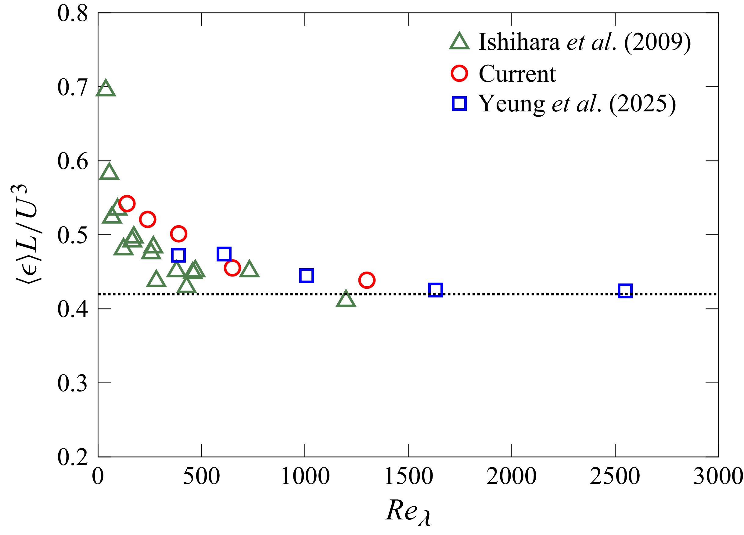


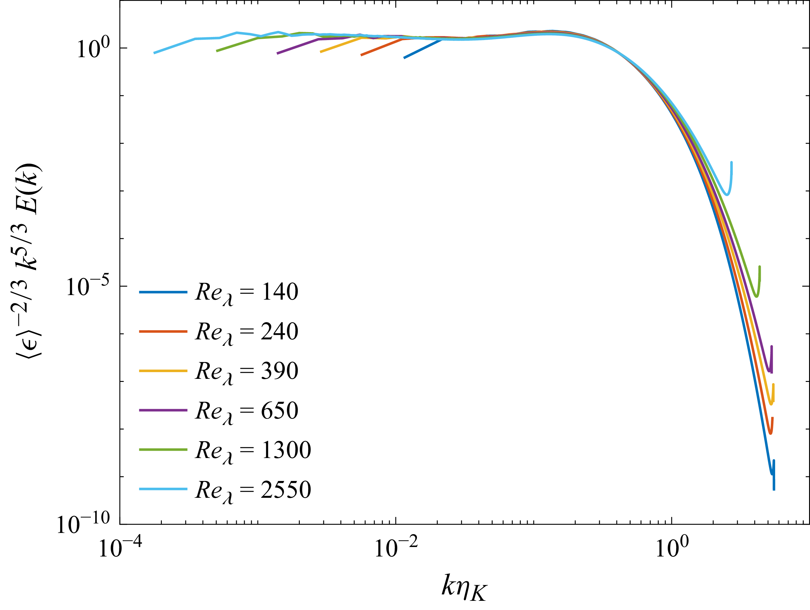


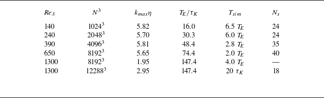


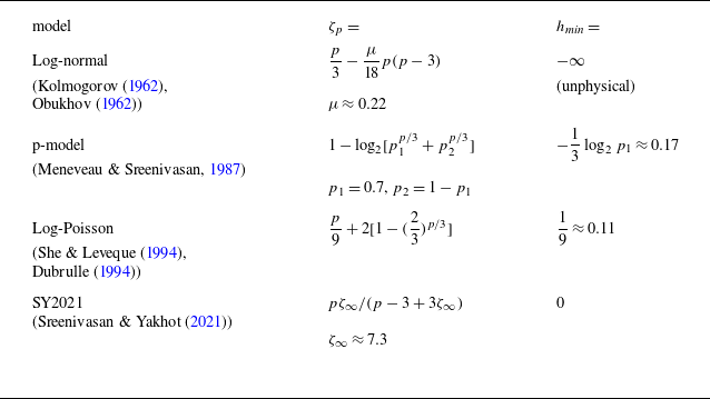


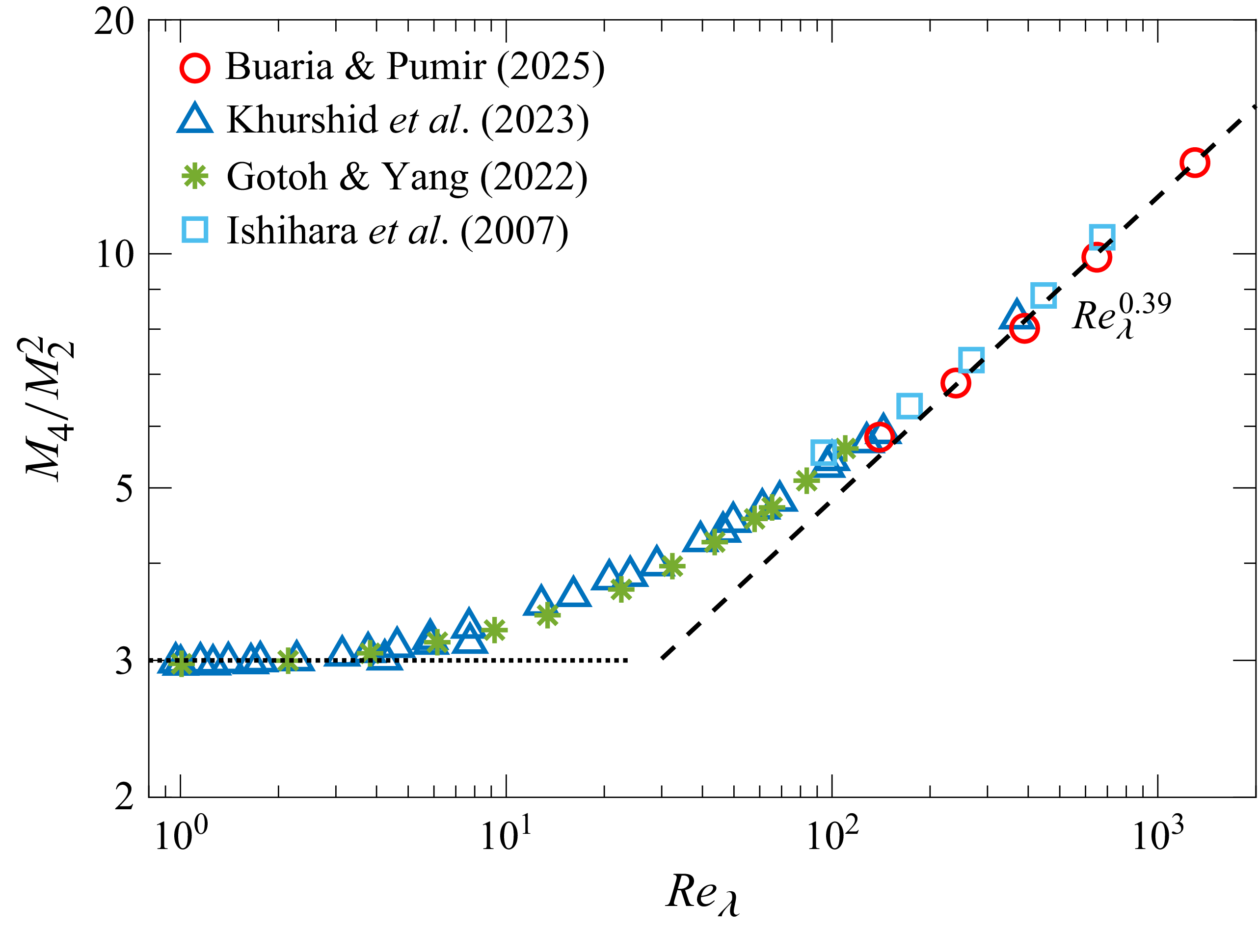


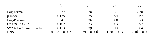


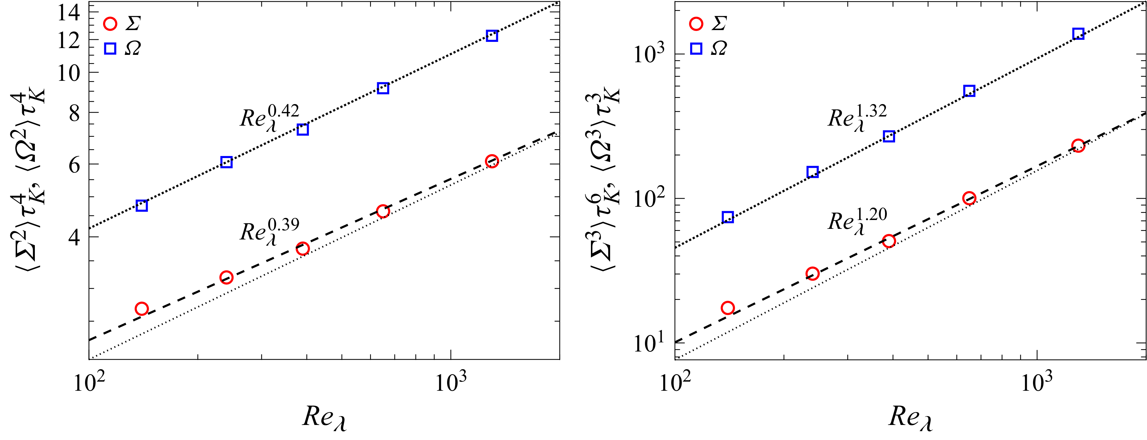


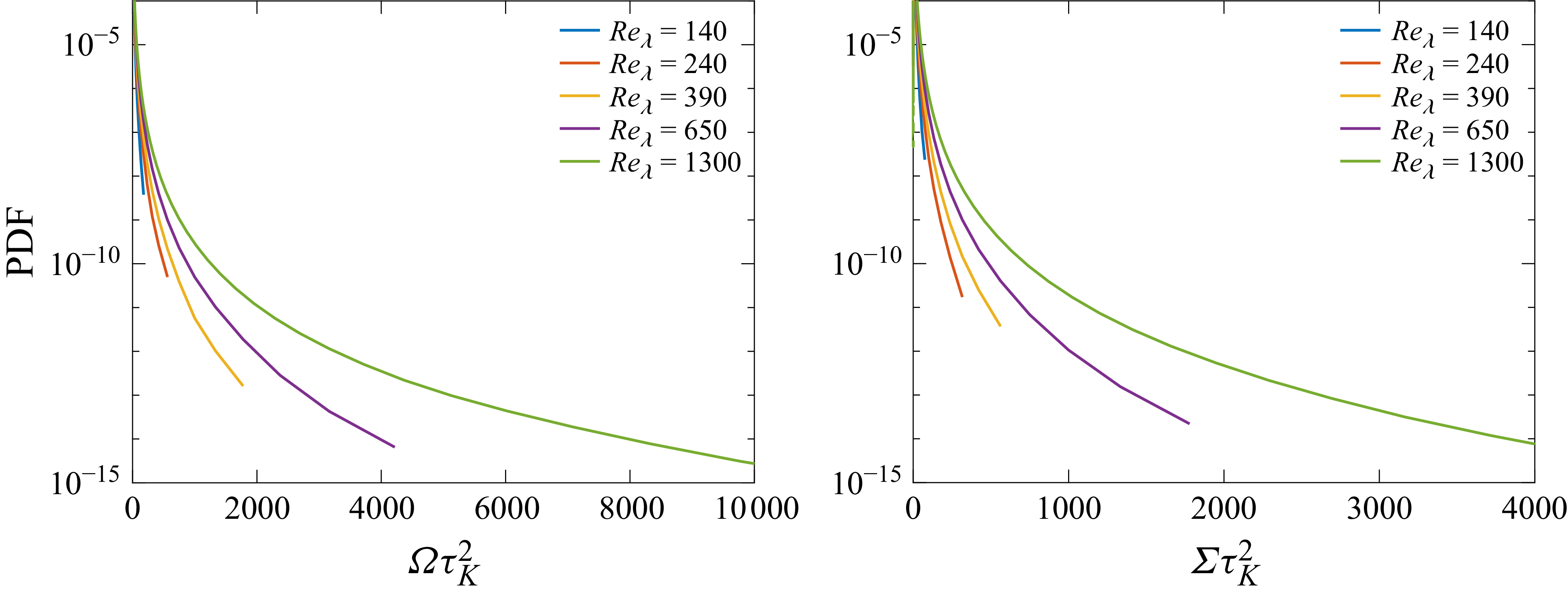


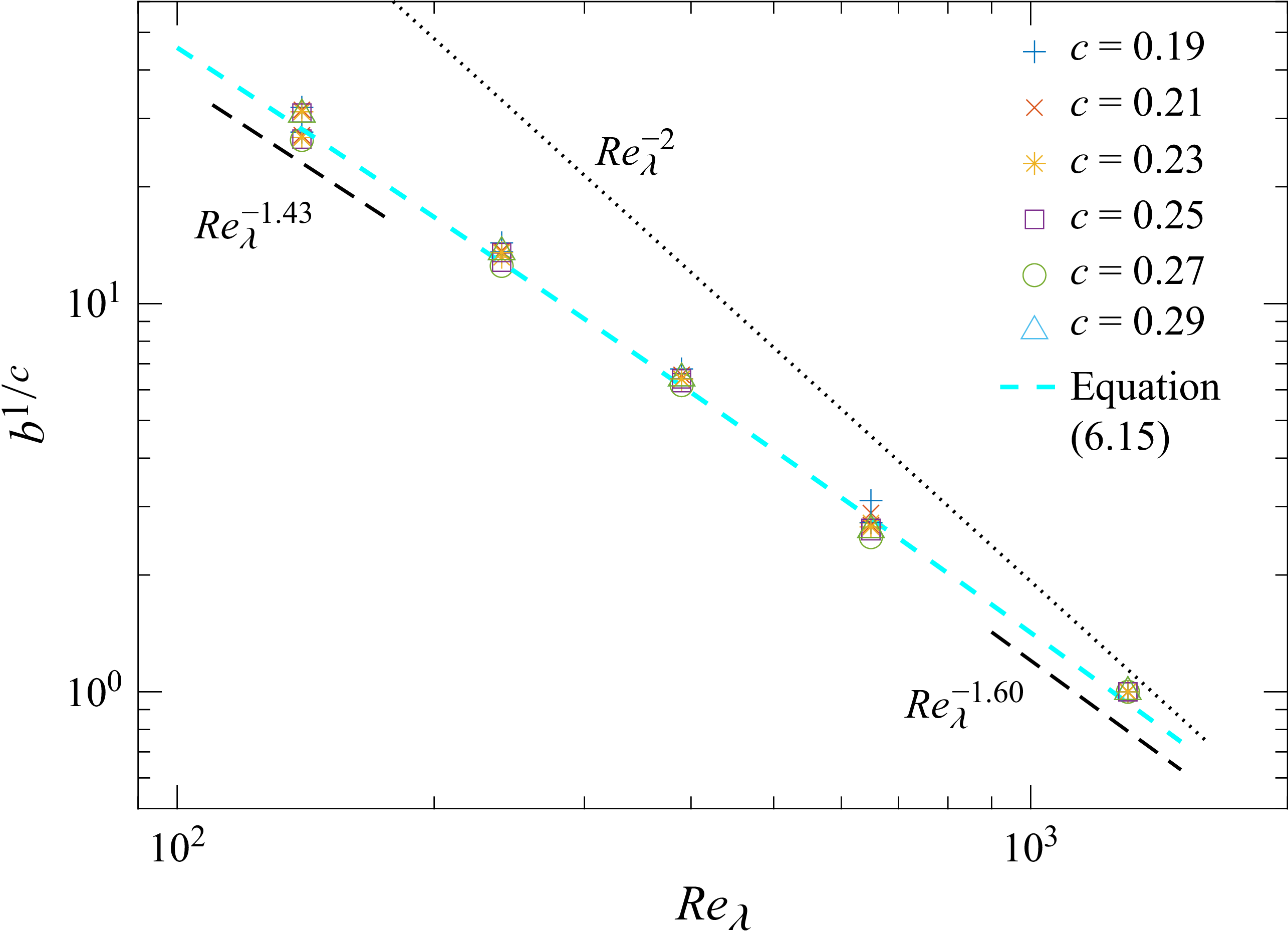


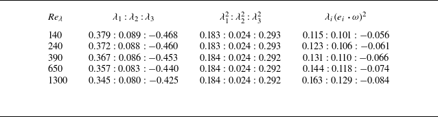


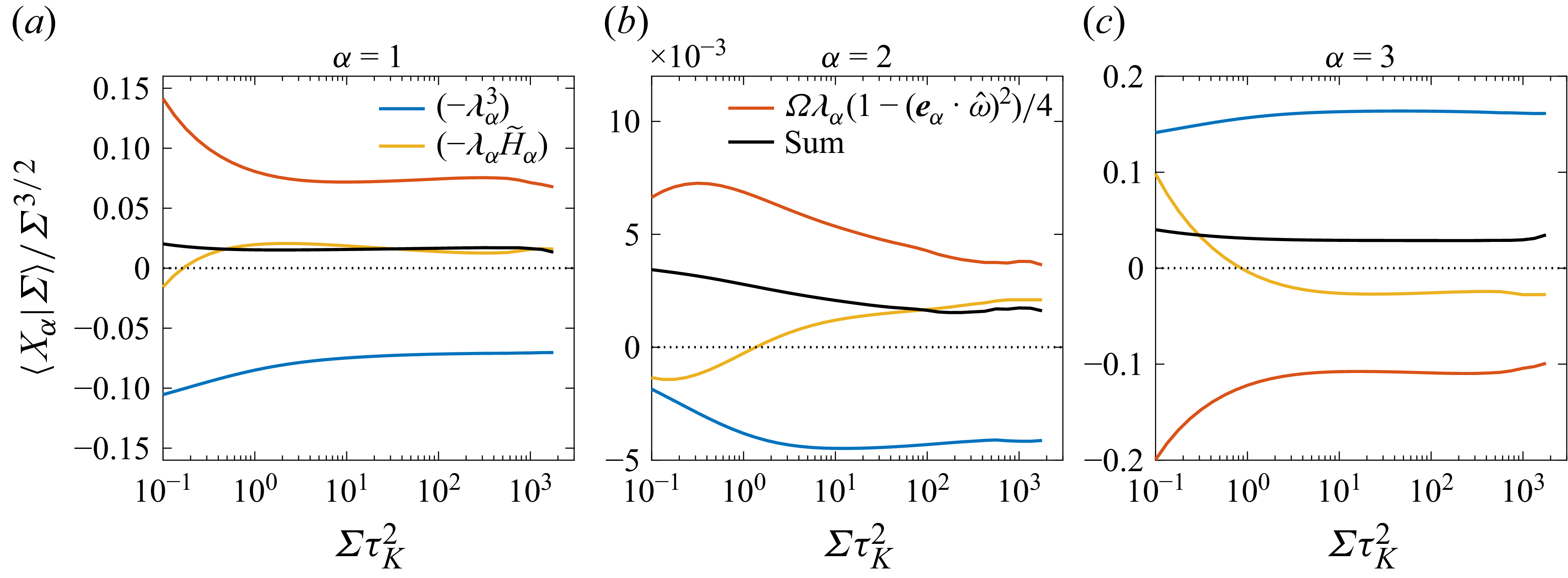

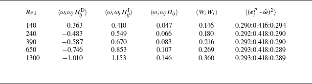


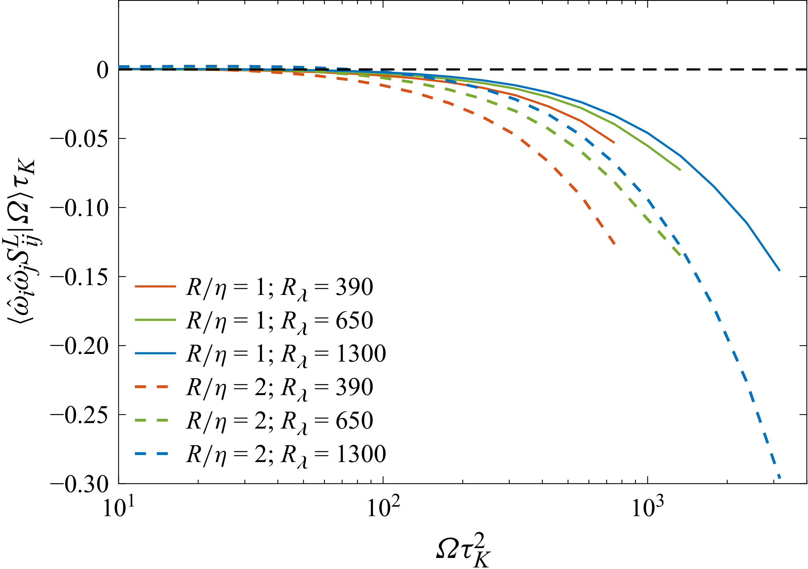


 Open access