


1. Introduction
Rayleigh–Bénard convection, a buoyancy-driven flow in a horizontal fluid layer heated from below and cooled from above, is one of the most canonical flows widely observed in nature, and also in engineering applications. The effect of buoyancy on a flow is characterised by the Rayleigh number  $Ra$. When $Ra$ exceeds a certain critical value $Ra_{c}$, the thermal conduction state becomes unstable and two-dimensional (2-D) steady convection rolls appear (Drazin & Reid Reference Drazin and Reid1981). At a higher $Ra$, the convection becomes time-dependent and subsequently exhibits turbulent states with multi-scale thermal and vortex structures. One of the primary interests in the Rayleigh–Bénard problem is the scaling of turbulent heat transfer with $Ra$, i.e. the dependence of the Nusselt number $Nu$ on $Ra$. Over half a century ago, Priestley (Reference Priestley1954) and Malkus (Reference Malkus1954) simultaneously and independently proposed $Nu\sim Ra^{1/3}$. Priestley derived the scaling from a similarity argument based on dimensional analysis by assuming that the heat flux is independent of the height of the fluid layer, $H$, while leaving the Prandtl number $Pr$ dependence unspecified. In contrast, Malkus obtained a scaling independent of $Pr$ based on a marginal stability argument. Later Malkus’ theory was reframed and developed by Howard (Reference Howard1966). Malkus (Reference Malkus1954) also raised a question for the upper limit of the heat transfer in thermal convection, and the upper bounds of $Nu\sim Ra^{1/2}$ were derived via variational approaches (Howard Reference Howard1963; Busse Reference Busse1969). In the 1990s, Doering & Constantin (Reference Doering and Constantin1996) derived a rigorous upper bound of $Nu\le 0.167Ra^{1/2}-1$ by employing a new variational approach called ‘the background method’ (Doering & Constantin Reference Doering and Constantin1992), and then the lowest asymptotic upper bound, $Nu-1=0.02634Ra^{1/2}$, was obtained by Plasting & Kerswell (Reference Plasting and Kerswell2003). Based on the mixing-length theory, apart from the upper-bound problems, a scaling of $Nu\sim Pr^{1/2}Ra^{1/2}$ was derived by Spiegel (Reference Spiegel1963). In 1961, his theory was already proposed as testified by Batchelor (Reference Batchelor1961) (see also Doering Reference Doering2019). Shortly afterwards, Kraichnan (Reference Kraichnan1962) modified Spiegel's theory, and predicted $Nu\sim Pr^{1/2}Ra^{1/2}(\ln Ra)^{-3/2}$ for a sufficiently large $Ra$, as a scaling in an asymptotic state with turbulent boundary layers. The logarithmic correction possibly varies from $(\ln Ra)^{-3/2}$ to $(\ln Ra)^{-3}$ (Chavanne et al. Reference Chavanne, Chilla, Castaing, Hebral, Chabaud and Chaussy1997); $Nu\sim Pr^{1/2}Ra^{1/2}$ is currently called ‘ultimate’ scaling. In conventional turbulent Rayleigh–Bénard convection, however, the ultimate scaling has not been observed yet. A prominent experiment by Niemela et al. (Reference Niemela, Skrbek, Sreenivasan and Donnelly2000) for a very high $Ra$ exhibits $Nu\sim Ra^{0.31}$ even at $Ra\sim 10^{17}$. A recent numerical simulation by Iyer et al. (Reference Iyer, Scheel, Schumacher and Sreenivasan2020) up to $Ra=10^{15}$, in a slender cylindrical container with an aspect ratio of $1/10$, exhibits $Nu\sim Ra^{0.33}$. In the 1990s, Shraiman & Siggia (Reference Shraiman and Siggia1990) deduced $Nu\sim Pr^{-1/7}Ra^{2/7}$ by assuming the existence of turbulent boundary layers. In the 2000s, Grossmann & Lohse (Reference Grossmann and Lohse2000, Reference Grossmann and Lohse2001, Reference Grossmann and Lohse2002, Reference Grossmann and Lohse2004) proposed a unifying scaling law of global properties for $Ra$ and $Pr$, based on decomposing the total scalar and energy dissipation into contributions from the bulk region and the boundary layer. Their scaling argument results in two equations for the Nusselt number $Nu(Ra,Pr)$ and the Reynolds number $Re(Ra,Pr)$ with six adjustable parameters, and they are determined to fit experimental and numerical data. Many experiments and numerical simulations have demonstrated the validity of this scaling law (Ahlers, Grossmann & Lohse Reference Ahlers, Grossmann and Lohse2009; Stevens et al. Reference Stevens, van der Poel, Grossmann and Lohse2013). Per the argument, the scaling $Nu\sim Ra^{1/3}$ is derived in the high- $Ra$ regime $10^{8}\lesssim Ra\lesssim 10^{14}$ for $Pr\sim 1$. The transition to the ultimate scaling is also predicted for $Ra\gtrsim 10^{14}$; however, the local effective behaviour is represented by $Nu\approx cRa^{0.38}$, where $c$ is a fitting constant, due to logarithmic corrections (Grossmann & Lohse Reference Grossmann and Lohse2011). Although some results have shown the transition to $Nu\sim Ra^{0.38}$, the high- $Ra$ scaling is still being discussed (Chillà & Schumacher Reference Chillà and Schumacher2012; Zhu et al. Reference Zhu, Mathai, Stevens, Verzicco and Lohse2018; Doering, Toppaladoddi & Wettlaufer Reference Doering, Toppaladoddi and Wettlaufer2019a,Reference Doering, Toppaladoddi and Wettlauferb). In contrast, for $10^{8}\lesssim Ra\lesssim 10^{11}$, a considerable amount of turbulent data exhibit the classical scaling $Nu\sim Ra^{1/3}$ (e.g. Niemela & Sreenivasan Reference Niemela and Sreenivasan2006; He et al. Reference He, Funfschilling, Nobach, Bodenschatz and Ahlers2012).
Recently, Waleffe, Boonkasame & Smith (Reference Waleffe, Boonkasame and Smith2015) found a scaling of  $Nu=0.115Ra^{0.31}$ in 2-D steady Rayleigh–Bénard convection for $10^7\lesssim Ra\lesssim 10^9$ and $Pr=7$ (see also Sondak, Smith & Waleffe Reference Sondak, Smith and Waleffe2015). In their work, 2-D steady solutions were obtained to maximise $Nu$ by optimising the horizontal periods. The scaling is achieved by a family of 2-D solutions with a horizontal period that decreases with increasing $Ra$. Interestingly, the scaling is quite similar to the three-dimensional (3-D) turbulent data fit $Nu=0.105Ra^{0.312}$ (He et al. Reference He, Funfschilling, Nobach, Bodenschatz and Ahlers2012). Although the result suggests that simple and coherent structures can capture the essence of convective turbulence, it does not imply that this can be realised by any single 2-D steady solution with a fixed horizontal period (fundamental wavelength). More recently, a wall-to-wall optimal transport problem, which is a variational problem for finding a divergence-free velocity field optimising scalar transport between two parallel plates, has been discussed (Hassanzadeh, Chini & Doering Reference Hassanzadeh, Chini and Doering2014; Tobasco & Doering Reference Tobasco and Doering2017; Doering & Tobasco Reference Doering and Tobasco2019). Motoki, Kawahara & Shimizu (Reference Motoki, Kawahara and Shimizu2018a) also numerically obtained 3-D time-independent velocity fields to be the optimal states maximising heat transfer between two isothermal no-slip parallel plates under the constraint of fixed total enstrophy. The optimal states exhibit ultimate scaling, which is quite close to the lowest rigorous upper bound obtained by Plasting & Kerswell (Reference Plasting and Kerswell2003), and lead to hierarchical self-similar vortex structures. In the optimised 3-D velocity fields, smaller and stronger vortices appear closer to the walls as the total enstrophy increases. In velocity fields numerically optimised within a 2-D field, the emergence of such hierarchical flow structures has not been observed (Souza, Tobasco & Doering Reference Souza, Tobasco and Doering2020). Although the 3-D optimal state needs an external body force other than buoyancy, we proved that the optimal state found by Motoki et al. (Reference Motoki, Kawahara and Shimizu2018a) could continuously connect to a steady solution of the Boussinesq equations using the homotopy continuation method (see appendix A).
In this paper, we discuss the connected 3-D steady solution. In the Rayleigh–Bénard convection between horizontal boundaries, a 3-D steady solution with convection cells also bifurcates from the conduction state at the same critical value of  $Ra$ as the 2-D steady solution (see figure 1). This is because convection rolls in any horizontal direction can exist simultaneously. Although the 3-D solution is not stable, it exists even at a high $Ra$. We demonstrate the ability of this invariant solution to capture key statistical features, as well as coherent thermal and flow structures in turbulent Rayleigh–Bénard convection. We then discuss the hierarchical multi-scale vortex structures and energy transfer in the 3-D steady solution.
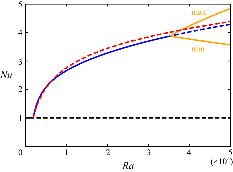
Nusselt number  $Nu$ as a function of Rayleigh number $Ra$. The red and blue curves represent the 3-D steady solution in the square periodic domain and 2-D steady solution with $L/H={\rm \pi} /2$ for $Pr=1$ bifurcating from the conduction state (black) at $Ra\approx 1879$, respectively. The orange curves show the maximum and minimum values of $Nu$ in the 3-D time-periodic solution. The dashed lines denote unstable solutions.
The remainder of the paper is organised as follows. In § 2, we introduce the governing equations, boundary conditions and dimensionless parameters to characterise the thermal convection. We then describe the numerical procedures to obtain nonlinear solutions. The statistical properties and spatial structures of the 3-D steady solution are presented in § 3, and the hierarchical vortex structures are discussed in § 4. Finally, a summary and conclusions are presented in § 5. In appendix A, we present the homotopy continuation analysis from the 3-D optimal solution of the Euler–Lagrange equations for the wall-to-wall optimal transport problem to the present 3-D steady solution of the Boussinesq equations. The parameter dependence of the 3-D steady solution and the adequacy of the spatial resolution are discussed in appendix B.
2. Boussinesq equations and numerical methods
Let us consider a fluid layer between two horizontal plates heated from below and cooled from above. We employ the Oberbeck–Boussinesq approximation, wherein the density variations are only significant in the buoyancy term. The time evolutions of velocity field  ${\boldsymbol {u}}({\boldsymbol {x}},t)=u{\boldsymbol {e}}_{x}+v{\boldsymbol {e}}_{y}+w{\boldsymbol {e}}_{z}$ and temperature field $T({\boldsymbol {x}},t)$ are described by the Boussinesq equations
 \begin{gather} \boldsymbol{\nabla}\boldsymbol{\cdot}{\boldsymbol{u}}=0, \end{gather}
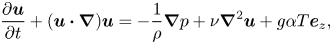 \begin{gather}\frac{\partial {\boldsymbol{u}}}{\partial t}+({\boldsymbol{u}}\boldsymbol{\cdot}\boldsymbol{\nabla}){\boldsymbol{u}}=-\frac{1}{\rho}\boldsymbol{\nabla} p+\nu\boldsymbol{\nabla}^{2}{\boldsymbol{u}}+g\alpha T{\boldsymbol{e}}_{z}, \end{gather}
 \begin{gather}\frac{\partial T}{\partial t}+({\boldsymbol{u}}\boldsymbol{\cdot}\boldsymbol{\nabla})T=\kappa\boldsymbol{\nabla}^{2}T, \end{gather}
where  $p({\boldsymbol {x}},t)$ is pressure and $\rho , \nu , g, \alpha$ and $\kappa$ are the mass density, kinematic viscosity, acceleration due to gravity, volumetric thermal expansivity and thermal diffusivity, respectively. Vectors ${\boldsymbol {e}}_{x}$ and ${\boldsymbol {e}}_{y}$ are mutually orthogonal unit vectors in the horizontal directions, while ${\boldsymbol {e}}_{z}$ is a unit vector in the vertical direction. The two no-slip and impermeable horizontal plates are positioned at $z=0$ and $z=H$, and the top (or bottom) wall surface is held at a lower (or higher) constant temperature:
 \begin{equation} \boldsymbol{u}(z=0)=\boldsymbol{u}(z=H)=\boldsymbol{0};\quad T(z=0)=\Delta T>0,\quad T(z=H)=0. \end{equation}
The velocity and temperature fields are supposed to be periodic in the  $x$ and $y$ directions with the same period $L_{x}=L_{y}=L$. The thermal convection is characterised by the Rayleigh number $Ra$ and the Prandtl number $Pr$:
$Pr$:
 \begin{equation} Ra=\frac{g\alpha\Delta T H^{3}}{\nu\kappa},\quad Pr=\frac{\nu}{\kappa}. \end{equation}
The vertical heat flux is quantified by the Nusselt number:
 \begin{equation} Nu=\frac{-\kappa{\langle \partial T/\partial z \rangle}_{xyt}+{\langle wT \rangle}_{xyt}}{\kappa\Delta T/H}=1+\frac{H}{\kappa\Delta T}{\left\langle wT \right\rangle}_{xyzt}, \end{equation}
where  $\langle \cdot \rangle _{xyt}$ and $\langle \cdot \rangle _{xyzt}$ represent the horizontal and time average and the volume and time average, respectively. The second equality is given by the volume and time average of (2.3).
Equations (2.1)–(2.3) are discretised employing a spectral Galerkin method based on the Fourier series expansion in the periodic horizontal directions and the Chebyshev polynomial expansion in the vertical direction. The nonlinear terms are evaluated using a spectral collocation method. Aliasing errors are removed with the aid of the  $2/3$ (or $1/2$) rule for the Fourier (or Chebyshev) transform. Time advancement is performed with the Crank–Nicholson scheme and the second-order Adams–Bashforth scheme for the diffusion terms and the rest, respectively. The nonlinear steady solutions are obtained using the Newton–Krylov iteration (for more details, see § 3 and appendix A in Motoki, Kawahara & Shimizu (Reference Motoki, Kawahara and Shimizu2018b)).
In this paper, we present the steady solution and the turbulent states in the horizontally square periodic domain with  $L/H={\rm \pi} /2\approx 1.57$ for $Pr=1$. The domain is the same as that of the optimal states derived by Motoki et al. (Reference Motoki, Kawahara and Shimizu2018a). The numerical process is conducted on $128^{3}$ grid points for $Ra<10^7$ and $256^{3}$ grid points for $Ra\ge 10^7$. In the smaller (or larger) domain with $L/H=1$ (or $L/H=2{\rm \pi} /3.117\approx 2.02$), we have confirmed that the effects of the domain size on the heat flux and the spatial structures are insignificant, which is described in the following sections. The domain size dependence is shown in appendix B with the Prandtl number dependence and the adequacy of the spatial resolution.
All the 3-D steady solutions presented in this paper satisfy the  ${\rm \pi} /2$-rotation symmetry
 \begin{equation} [u,v,w,T](x,y,z)=[v,-u,w,T](\,y,-x,z) \end{equation}
as well as the reflection symmetry
 \begin{equation} [u,v,w,T](x,y,z)=[-u,v,w,T](-x,y,z) \nonumber\\ =[u,-v,w,T](x,-y,z) \end{equation}
and the shift-and-reflection symmetry
 \begin{equation} [u,v,w,T](x,y,z)=[u,v,-w,1-T](x+L/2,y+L/2,1-z). \end{equation}
These symmetries are not imposed on the solutions explicitly at  $Ra\lesssim 10^6$. At $Ra\sim 10^{7}$, we impose the symmetries (2.7)–(2.9) in order to reduce the computational degrees of freedom.
3. Three-dimensional steady solution
3.1. The  $Nu$–$Ra$ scaling


The 3-D and 2-D steady solutions in the domain with  $L/H={\rm \pi} /2$ for $Pr=1$ bifurcate from the conduction state at $Ra\approx 1879$, as shown in figure 1. The 2-D roll solution is stable up to $Ra\approx 3.55\times 10^{4}$, and subsequently a time-periodic 3-D solution appears (the stable periodic solution has been obtained by the time evolution). Figure 2 presents $Nu$ in the 3-D and 2-D steady solutions as a function of $Ra$ at a higher $Ra$. The red line shows the 3-D steady solution, and the open and filled circles represent the present turbulent data in the horizontally square periodic domain and the experimental data in a cylindrical container (Niemela & Sreenivasan Reference Niemela and Sreenivasan2006), respectively. The blue circles represent the 2-D optimised steady solutions for $Pr=1$ obtained by Sondak et al. (Reference Sondak, Smith and Waleffe2015). Although the 3-D steady solution at high $Ra$ exhibits smaller $Nu$ than the 2-D optimised solutions, it maintains larger $Nu$ than the turbulent states even at $Ra\sim 10^{7}$. The inset shows $Nu$ compensated by $Ra^{\gamma }$. The scaling exponent $\gamma$ of turbulent states shows $2/7$ for $Ra\lesssim 10^{7}$; at higher $Ra$, it changes to $0.31$. Such a transition has been experimentally and numerically observed for $Pr\sim 1$ (Castaing et al. Reference Castaing, Gunaratne, Heslot, Kadanoff, Libchaber, Thomae, Wu, Zaleski and Zanetti1989; Silano, Sreenivasan & Verzicco Reference Silano, Sreenivasan and Verzicco2010). The exponent of the heat flux in the 3-D steady solution is greater than $2/7$ but less than $1/3$, with $0.31$ being the closest, whereas that in the 2-D steady solution with fixed $L/H={\rm \pi} /2$ (blue line) is smaller than $2/7$. The bumps in the 3-D steady solution correspond to the remarkable changes in the thermal and flow structures, which will be shown in § 3.3. At $Ra\sim 10^{4}$ the heat flux of the 3-D steady solution surpasses maxima in the 2-D steady solutions. As shown in appendix B, the 3-D steady solution with the smaller horizontal period ( $L/H=1$) shows larger $Nu$ at $Ra\sim 10^{5}$. The results imply that a family of the 3-D steady solutions with optimised horizontal periods might achieve maximal heat transfer in the steady Rayleigh–Bénard convection. The orange dashed line indicates the optimal scaling $Nu-1=0.0236Ra^{1/2}$ (Motoki et al. Reference Motoki, Kawahara and Shimizu2018a) given by the 3-D optimal states maximising the wall-to-wall transport, and it is quite close to the rigorous upper bound, $Nu-1=0.02634Ra^{1/2}$ (Plasting & Kerswell Reference Plasting and Kerswell2003). Although the 3-D optimal states exhibiting significantly high heat flux require an external body force different from buoyancy, the optimal state can be continuously connected to the present 3-D steady solution of the full Boussinesq equations by a homotopy from the body force to the buoyancy, as shown in appendix A.
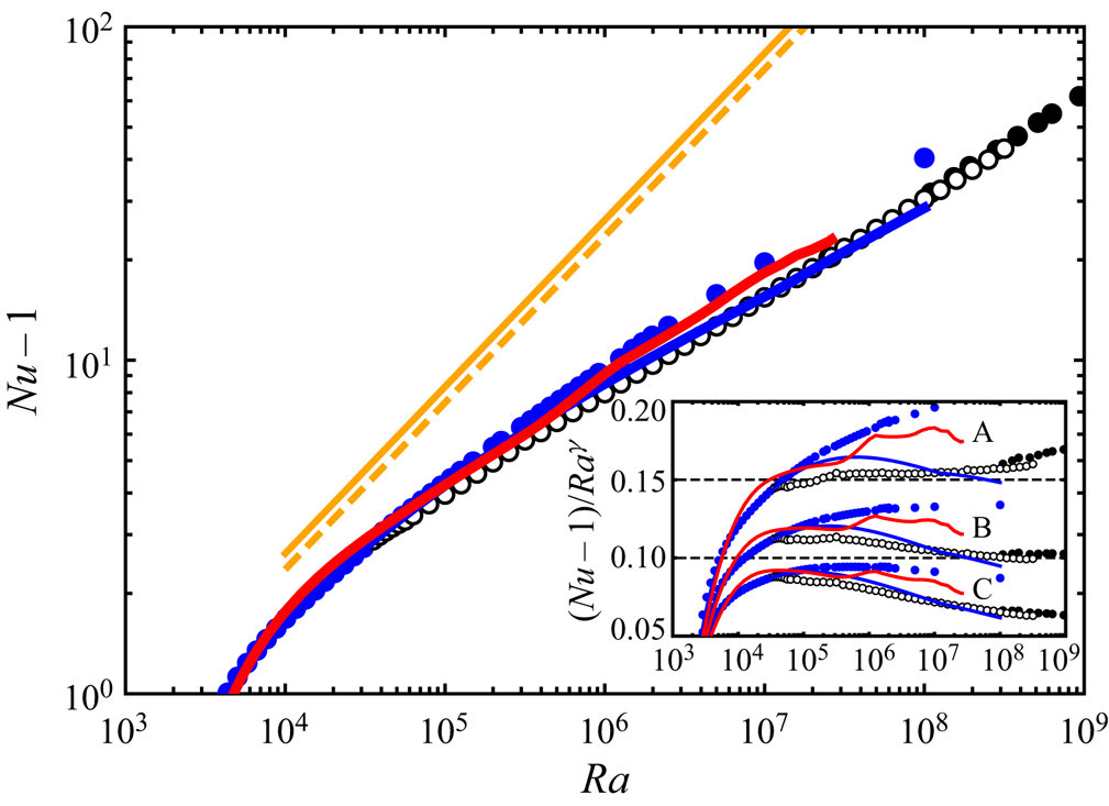
Nusselt number  $Nu-1$ as a function of Rayleigh number $Ra$. The red and blue solid lines represent the 3-D and 2-D steady solutions, respectively. The open black circles represent the present turbulent data obtained in the horizontally square periodic domain, and the filled ones are the experimental turbulent data in a cylindrical container (Niemela & Sreenivasan Reference Niemela and Sreenivasan2006). The blue filled circles indicate 2-D optimised steady solutions for $Pr=1$ obtained by Sondak et al. (Reference Sondak, Smith and Waleffe2015). The orange solid and dashed lines indicate the upper bound $Nu-1=0.02634Ra^{1/2}$ (Plasting & Kerswell Reference Plasting and Kerswell2003) and the optimal scaling $Nu-1=0.0236Ra^{1/2}$, respectively, evaluated from the wall-to-wall optimal transport states (Motoki et al. Reference Motoki, Kawahara and Shimizu2018a). The inset shows $Nu$ compensated by $Ra^{\gamma }$: $\gamma =2/7$ (plot A); $\gamma =0.31$ (plot B); $\gamma =1/3$ (plot C).
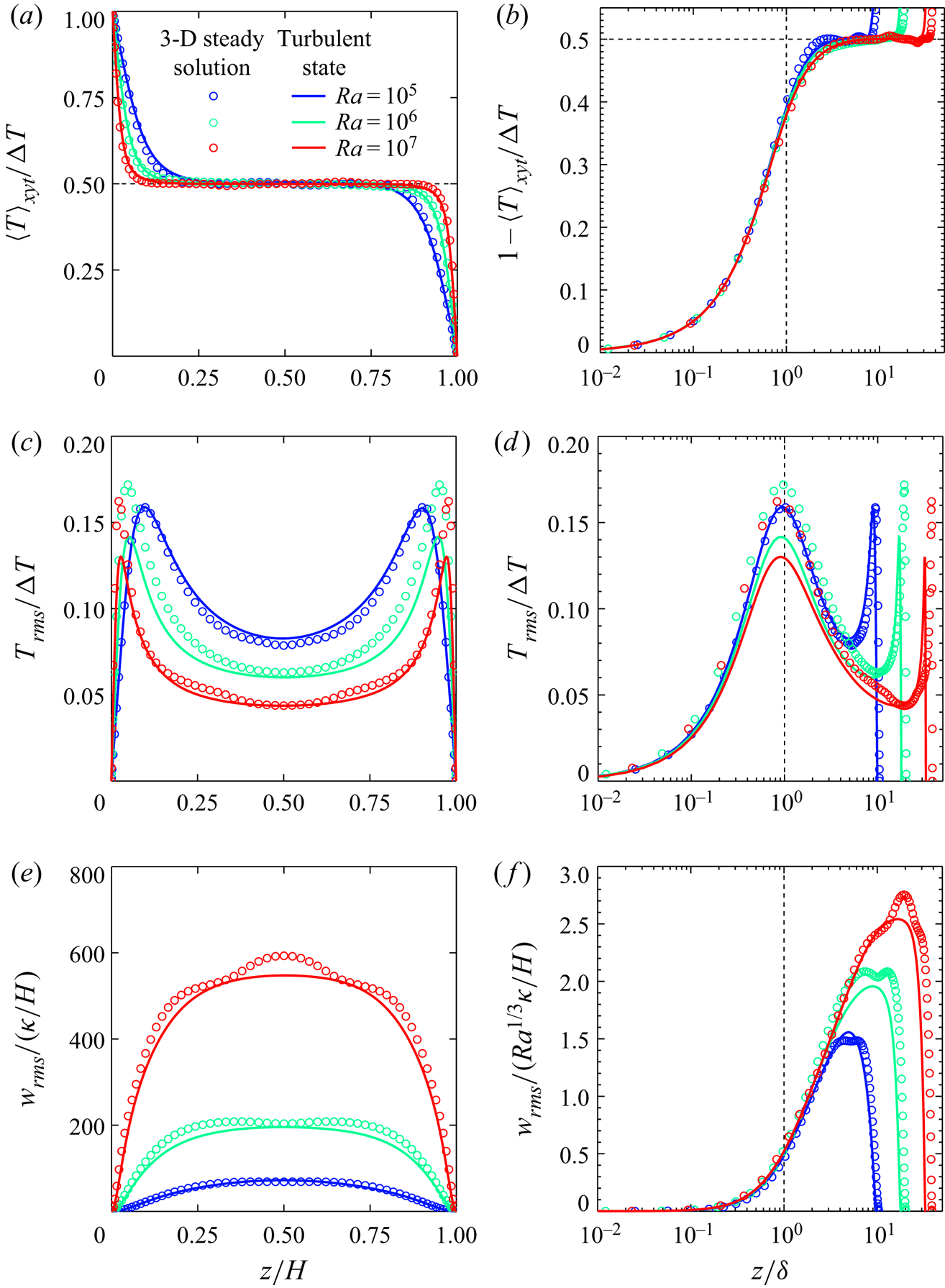
3.2. Mean temperature and root-mean-square profiles
Figure 3 compares the mean temperature  ${\langle T \rangle }_{xyt}$, root-mean-square (RMS) temperature $T_{rms}={\langle {(T-{\langle T \rangle }_{xyt})}^{2} \rangle }_{xyt}^{1/2}$ and RMS vertical velocity $w_{rms}={\langle w^{2} \rangle }_{xyt}^{1/2}$ for the 3-D steady solution with those for the turbulent states at $10^{5}\le Ra\le 10^{7}$. In figure 3(b,d,f) the distance to the wall, $z$, is normalised by $\delta$, where $\delta$ is the thermal conduction layer thickness given by $\delta /H=1/(2Nu)$. The mean temperature in the 3-D steady solution well follows that in the turbulent states; furthermore, the corresponding RMS values are also in good agreement with each other. In the bulk region, all mean temperature profiles are flattened, as a result of the nearly complete mixing by large-scale circulation. The temperature difference $\Delta T/2$ exists only at the thermal conduction layer, $0\le z\lesssim 2\delta /H=1/Nu$, and $T_{rms}$ exhibits a peak at $z/\delta \approx 1$. If the advection, diffusion and buoyancy terms in the Navier–Stokes equation (2.2) at the conduction layer are balanced as
 \begin{equation} \frac{w'^{2}}{\delta}\sim\nu\frac{w'}{\delta^{2}}\sim g\alpha\Delta T \end{equation}
(the balance between the advection and diffusion terms is given by that in the energy equation (2.3) for  $\nu \sim \kappa$), the near-wall vertical velocity would then be
 \begin{equation} w'\sim{(g\alpha\Delta T\delta)}^{1/2}\sim Ra^{1/3}\frac{\kappa}{H}, \end{equation}
yielding the scaling law
 \begin{equation} Nu\sim Ra^{1/3} \end{equation}
(Kawano et al. Reference Kawano, Motoki, Shimizu and Kawahara2021), which has been given by Malkus’ theory (Malkus Reference Malkus1954) and the argument of Grossmann & Lohse (Reference Grossmann and Lohse2000). As shown in figure 3(f), the RMS vertical velocity  $w_{rms}$ scales as $Ra^{1/3}\kappa /H$ near the wall $z/\delta \sim 1$.
(a,b) Mean temperature, (c,d) RMS temperature and (e,f) RMS vertical velocity as a function of (a,c,e)  $z/H$ and (b,d,f) $z/\delta$ in the 3-D steady solution and the turbulent state. Here $\delta$ is the thermal conduction layer thickness that scales as $\delta /H=1/(2Nu)$.
In the bulk region, where the effects of viscosity or thermal conduction are insignificant, the advection and buoyancy terms are balanced as
 \begin{equation} \frac{U_{b}^{2}}{H}\sim g\alpha\Delta T', \end{equation}
and the dominance of convective heat transfer in bulk and the scaling (3.3) give us
 \begin{equation} \frac{U_{b}\Delta T'}{\kappa \Delta T/H}\sim Ra^{1/3} \end{equation}
(Kawano et al. Reference Kawano, Motoki, Shimizu and Kawahara2021). Equations (3.4) and (3.5) yield the bulk velocity scales as
 \begin{equation} U_{b}\sim Pr^{-2/3}Ra^{4/9}\nu/H. \end{equation}
The Reynolds number based on  $U_{b}$ scales with $Pr^{-2/3}Ra^{4/9}$, exhibiting consistency with the scaling suggested by Grossmann & Lohse (Reference Grossmann and Lohse2000) when both energy and scalar dissipation are bulk-dominated. Figure 4 shows the Reynolds number $Re$ defined as
 \begin{equation} Re=\frac{{\langle w^{2} \rangle}_{xyzt}^{1/2}H}{\nu} \end{equation}
as a function of  $Ra$. The Reynolds number $Re$ of the 3-D steady solution is comparable with that of the turbulent states exhibiting ${Re}\sim Ra^{4/9}$ at a high $Ra$. In contrast, the 2-D steady solution with fixed $L/H={\rm \pi} /2$ seems to approach $Re\sim Ra^{1/2}$, implying that $\langle w^{2}\rangle _{xyzt}^{1/2}$ scales with the buoyancy-induced terminal velocity $U={(g\alpha \Delta TH)}^{1/2}$.
Reynolds number  $Re$ as a function of Rayleigh number $Ra$. The red and blue solid lines represent the 3-D and 2-D steady solutions, respectively. The open circles represent the present turbulent data obtained in the horizontally square periodic domain. The inset shows $Nu$ compensated by $Ra^{\gamma }$: $\gamma =4/9$ (plot A); $\gamma =1/2$ (plot B).
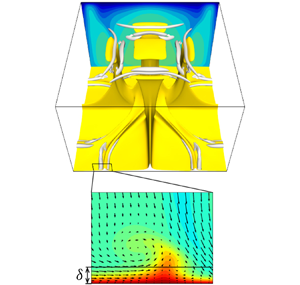
3.3. Thermal and flow structures
Figure 5 visualises the thermal and flow structures in the 3-D steady solution and the turbulent state. The yellow objects represent the isosurfaces of temperature  $T/\Delta T=0.6$, representing high-temperature plumes; the grey objects represent the vortex structures visualised by the positive second invariant of the velocity gradient tensor
 \begin{equation} Q=-\frac{1}{2}\frac{\partial u_{i}}{\partial x_{j}}\frac{\partial u_{j}}{\partial x_{i}}. \end{equation}
At  $Ra=10^{5}$ (figure 5a), the 3-D steady solution consists of large-scale thermal plumes as well as accompanying near-wall small-scale plume and vortex structures near the vertical planes $x/H=0$ and $y/H=0$. As $Ra$ for the 3-D steady solution increases, smaller thermal plume structures (and relevant smaller and stronger tube-like vortex structures) appear near the walls without affecting the already existing large-scale structures. As $Ra$ increases from $10^{5}$ to $10^{6}$, thermal and vortex structures newly emerge along the diagonals $y={\pm }x$ near the walls (figure 5b). As $Ra$ increases further from $10^{6}$ to $10^{7}$, smaller-scale structures appear along $x/H=\pm {\rm \pi}/8$ and $y/H={\pm }{\rm \pi} /8$ near the walls, and the large secondary plumes approach the opposite wall (figure 5c). The bumps of $Nu$ seen in figure 2 correspond to these remarkable changes in the thermal and vortex structures.
Thermal and flow structures in (a–c) the 3-D steady solution and (d) the turbulent state at (a)  $Ra=10^5$, (b) $Ra=10^6$ and (c,d) $Ra=10^7$. The yellow and grey objects represent the isosurfaces of the temperature $T/\Delta T=0.6$ and the positive second invariant of the velocity gradient tensor, (a) $Q/(\kappa ^2/H^4)=1.28\times 10^5$, (b) $Q/(\kappa ^2/H^4)=1.28\times 10^6$ and (c,d) $Q/(\kappa ^2/H^4)=8\times 10^7$, respectively. The contours represent temperature $T$ in the plane $y/H={\rm \pi} /4 (=-{\rm \pi} /4)$, and the velocity vectors $(u,w)$ in the enlarged views in (c,d) are superposed.
At  $Ra=10^7$ (figure 5c), we observe sheet-like thermal plumes with the smallest-scale vortices, which are quite similar to those observed in the snapshot of the turbulent state (figure 5d). The smallest-scale structures appear in the thermal conduction layer, and the sizes of the plumes and vortices scale with the thickness $\delta$. In 2-D optimised steady solutions (Sondak et al. Reference Sondak, Smith and Waleffe2015; Waleffe et al. Reference Waleffe, Boonkasame and Smith2015), the appearance of small-scale thermal and vortex structures has been observed with the shrinking horizontal period as $Ra$ increases, and the scaling $Nu\sim Ra^{0.31}$ is achieved by a family of solutions with smaller horizontal periods. It should be stressed that the single 3-D steady solution spontaneously reproduces the multi-scale coherent structures of convective turbulence.
4. Hierarchical vortices and energy transfer in wavenumber space
The 3-D steady solution is found to reproduce the near-wall coherent structures in convective turbulence; however, the flow in bulk should be addressed. The developed turbulence organises hierarchical coherent vortex structures of various scales (Goto, Saito & Kawahara Reference Goto, Saito and Kawahara2017; Motoori & Goto Reference Motoori and Goto2019). The smallest-scale vortex structures can still be extracted by employing the isosurface of  $Q$, as shown in figure 5; however, it is difficult to identify large- and intermediate-scale structures. To examine the hierarchy of multi-scale vortices in the 3-D steady solution, we consider coarse-graining the velocity field ${\boldsymbol {u}}$. The coarse-grained velocity field ${\boldsymbol {u}}^{*}$ is obtained using the Gaussian low-pass filter (Lozano-Durán, Holzner & Jimenez Reference Lozano-Durán, Holzner and Jimenez2016; Motoori & Goto Reference Motoori and Goto2019) as follows:
 \begin{equation} {\boldsymbol{u}}^{*}({\boldsymbol{x}})=\int_{V} {a}{\boldsymbol{u}}({\boldsymbol{x}}')\exp{\left\{ -{\left( \frac{{\rm \pi}\Delta r}{\sigma} \right)}^2 \right\}}\,\textrm{d}\kern0.7pt{\boldsymbol{x}}', \end{equation}
where  $\Delta r=|\boldsymbol {x}'-\boldsymbol {x}|$, $\sigma$ is the filter width and $a$ is a constant such that the integral of the kernel over the control volume $V$ is unity. In the wall-normal direction, the Gaussian filter is applied by reflecting it at the wall (Lozano-Durán et al. Reference Lozano-Durán, Holzner and Jimenez2016). Figure 6 shows hierarchical vortex structures in the 3-D steady solution at $Ra=2.6\times 10^7$. Non-filtered structures are shown in figure 6(a), and the isosurfaces of $Q$ of the filtered velocity ${{\boldsymbol {u}}}^{*}$ with $\sigma =H(=2L/{\rm \pi} ),L/2,L/4,L/8$ and $L/16$ are displayed in figure 6(b–f), respectively. The blue objects in figure 6(b) are the largest-scale structures corresponding to the large-scale circulation, whereas the red ones in figure 6(f) are the smallest-scale structures of size $\sigma /2=L/32\approx 2\delta$, which coincides with the size of vortices observed in the non-filtered field (figure 6a). The light blue, green and light red objects in figure 6(c,d,e) illustrate the intermediate-scale vortex structures of eight, four and two times the size of the smallest-scale vortices, respectively. The smaller-scale vortex structures exist closer to the wall, while the intermediate-scale ones are observed in the bulk region in figure 6(d,e).
Hierarchical vortex structures visualised by coarse-graining with Gaussian low-pass filter. (a) The yellow and red objects represent the isosurfaces of the non-filtered  $T/\Delta T=0.6$ and $Q/(\kappa ^2/H^4)=2\times 10^8$, respectively. (b–h) The vortex structures are visualised by the isosurfaces of $Q/(\kappa ^2/H^4)$ of the filtered velocity field with filter widths of $\sigma =H(=2L/{\rm \pi} )$ (blue), $\sigma =L/4$ (light blue), $\sigma =L/8$ (green), $\sigma =L/16$ (light red) and $\sigma =L/32$ (red); they are superposed in (g,h). The isosurface levels are (blue) $5\times 10^5$, (light blue) $4\times 10^6$, (green) $1.2\times 10^7$, (light red) $3\times 10^7$ and (red) $1.6\times 10^8$.
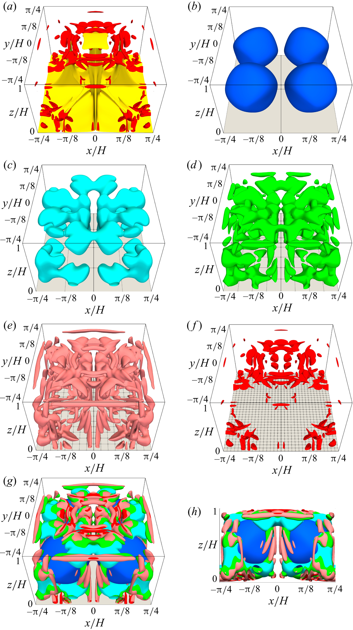
Figure 6(g,h) shows the superposed structures, and from their spatial distribution, it is conjectured that the bulk flow is composed of multi-scale coherent structures. Figure 7(a) shows the energy spectrum  $E(k,z)$ of the 3-D steady solution at the centre of the fluid layer, $z=H/2$, and the corresponding turbulence spectrum at $Ra=2.6\times 10^{7}$. The energy spectrum $E(k,z)$ is defined as
 \begin{equation} E(k,z)=\frac{L}{2{\rm \pi}}\sum_{k-{\Delta k}/{2}<|\boldsymbol{k}_{2D}|<k+{\Delta k}/{2}}\frac{1}{2}{\left\langle {|\tilde{\boldsymbol{u}}(\boldsymbol{k}_{2D},z)|}^{2} \right\rangle}_{t}, \end{equation}
where  $\tilde {(\cdot )}$ indicates the Fourier coefficients in the periodic ( $x$ and $y$) directions and ${\langle \cdot \rangle }_{t}$ represents the time average. Here $\boldsymbol {k}_{2D}=(k_{x},k_{y})$ and $k=|\boldsymbol {k}_{2D}|$ are the wavenumber vector and its magnitude, respectively, and $\Delta k=2{\rm \pi} /L$. The lateral and longitudinal axes are normalised by the kinematic viscosity $\nu$ and the energy dissipation rate
 \begin{equation} \varepsilon(z)=\frac{\nu}{2}{\left\langle {\left( \frac{\partial u_{i}}{\partial x_{j}}+\frac{\partial u_{j}}{\partial x_{i}} \right)}^{2} \right\rangle}_{xyt}, \end{equation}
which yield the Kolmogorov micro-scale length  $\eta=(\nu^3/\varepsilon)^{1/4}$. The spectra of the 3-D steady solution and turbulent state are in good agreement at high wavenumber $k\eta \gtrsim 10^{0}$. Furthermore, in the wavenumber band $2{\rm \pi} /(L/4)\lesssim k\eta \lesssim 2{\rm \pi} /(L/16)$, corresponding to the intermediate-scale range, the energy spectrum follows Kolmogorov's $-5/3$ power law, $E=C_{K}\varepsilon ^{2/3}k^{-5/3}$ (Kolmogorov Reference Kolmogorov1941), with the constant $C_{K}\approx 1.5$, which is consistent with that in the inertial subrange of high-Reynolds-number turbulence (Sreenivasan Reference Sreenivasan1995; Ishihara et al. Reference Ishihara, Morishita, Yokokawa, Uno and Kaneda2016).
(a) Energy spectrum  $E$ and (b) energy flux $\varPi$ at the centre of the fluid layer, $z=H/2$, in the 3-D steady solution (circles) and the turbulent state (lines) at $Ra=2.6\times 10^7$. The lateral and longitudinal axes are normalised by the kinematic viscosity $\nu$ and the energy dissipation rate $\varepsilon$ at $z=H/2$, which yield the Kolmogorov micro-scale length $\eta=(\nu^3/\varepsilon)^{1/4}$. The red dashed lines represent $E=1.5\varepsilon ^{2/3}k^{-5/3}$ and $\varPi /\varepsilon =1$, respectively. The light blue, green and light red colours indicate $k=2{\rm \pi} /(L/4)$, $2{\rm \pi} /(L/8)$ and $2{\rm \pi} /(L/16)$, respectively, normalised with $\eta$ in the 3-D steady solution, corresponding to the intermediate-scale structures shown in figure 6.
In figure 7(b), we show the energy flux in the wavenumber space,  $\varPi (k,z)$ (Mizuno Reference Mizuno2016), defined as
 \begin{gather} \varPi(k,z)=\sum_{k'\ge k}\sum_{k-{\Delta k}/{2}<|{\boldsymbol{k}}_{2D}|<k+{\Delta k}/{2}}T^{s}({\boldsymbol{k}}_{2D},z), \end{gather}
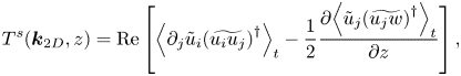 \begin{gather}T^{s}({\boldsymbol{k}}_{2D},z)=\mathrm{Re}\left[ {\left\langle \partial_{j}\tilde{u}_{i}{(\widetilde{u_{i}u_{j}})}^{{\dagger}ger} \right\rangle}_{t}-\frac{1}{2}\frac{\partial {\left\langle \tilde{u}_{j}{(\widetilde{u_{j}w})}^{{\dagger}ger} \right\rangle}_{t}}{\partial z} \right], \end{gather}
where  $(\partial _{1},\partial _{2},\partial _{3})=(\textrm {i}k_{x},\textrm {i}k_{y},\partial /\partial z)$ and ${\dagger}ger$ denotes the complex conjugate. Here $T^{s}(\boldsymbol {k}_{2D},z)$ represents the energy transfer between the Fourier modes, and the sum of all spectral components does not contribute to the total energy budget, i.e. $\sum _{\boldsymbol {k}_{2D}}T^{s}({\boldsymbol {k}}_{2D},z)=0$. In the intermediate-scale range, the energy flux exhibits positive values, that is, the energy is transferred from large to small scale, and it scales with the same order of energy dissipation rate.
In the optimised 2-D steady solution (Sondak et al. Reference Sondak, Smith and Waleffe2015; Waleffe et al. Reference Waleffe, Boonkasame and Smith2015), as  $Ra$ increases the horizontal scale of large-scale convective rolls reduces due to the shrinking of the horizontal period. The bulk flows at high $Ra$ diverge from those in the turbulent states, although it is intriguing that the optimised steady solutions exhibit the turbulent scaling $Nu\sim Ra^{0.31}$. Meanwhile, the 3-D steady solution reproduces not only the near-wall coherent structures but also the turbulence in the bulk of the Rayleigh–Bénard convection.
5. Summary and conclusions
We have discovered a 3-D steady solution to the Boussinesq equations, exhibiting a scaling of  $Nu\sim Ra^{0.31}$ and leading to multi-scale coherent structures, which are similar to those observed in turbulent Rayleigh–Bénard convection. The invariant solution bifurcates from the conduction state at $Ra\sim 10^3$, and it has been tracked up to $Ra\sim 10^7$ using the Newton–Krylov iteration. The heat flux of the 3-D steady solution can surpass maxima in the 2-D steady solutions (Sondak et al. Reference Sondak, Smith and Waleffe2015; Waleffe et al. Reference Waleffe, Boonkasame and Smith2015), and thus a family of the 3-D steady solutions with optimised horizontal periods might achieve maximal heat transfer in steady Rayleigh–Bénard convection. In contrast, in the 3-D steady solution with fixed horizontal periods, the horizontal-averaged temperature and the RMS of the temperature and velocity fluctuations are in good agreement with the horizontal and temporal averages obtained for the turbulent states. In the near-wall region of both the 3-D steady solution and the turbulent states, smaller-scale thermal plumes emerge with an increase in $Ra$. The size of the coherent thermal structures and relevant vortices is comparable with the thermal conduction layer thickness $\delta /H=1/(2Nu)$, and the RMS vertical velocity at $z/\delta \sim 1$ scales with the velocity scale $Ra^{1/3}\kappa /H$, corresponding to $Nu\sim Ra^{1/3}$. The Reynolds number $Re$ based on the RMS vertical velocity scales as $Re\sim Ra^{4/9}$, which is related to the scaling $Nu\sim Ra^{1/3}$. The bulk flow in the 3-D steady solution comprises hierarchical multi-scale vortices. We have extracted the large- and intermediate-scale vortex structures by employing the coarse-graining method. The ratio of the largest to the smallest length scales in the 3-D steady solution at $Ra=2.6\times 10^{7}$ is approximately $20$. The energy spectrum at the centre of the fluid layer shows good agreement with that of the turbulent state. In the intermediate-scale range, the spectrum follows $E=1.5\varepsilon ^{2/3}k^{-5/3}$, which is commonly observed in the inertial subrange of the developed turbulence. Furthermore, energy is transferred from large to small scales in the wavenumber space, and the energy flux balances the energy dissipation rate, in accordance with the Kolmogorov–Obukhov energy cascade view.
Recently, van Veen, Vela-Martín & Kawahara (Reference van Veen, Vela-Martín and Kawahara2019) have found a time-periodic solution that reproduces inertial range dynamics in a triply periodic turbulence driven by a constant body force of the Taylor–Green type. They have obtained the invariant solution by applying large-eddy simulation based on the Smagorinsky-type eddy-viscosity model. Meanwhile, by introducing the buoyant force, we have succeeded in finding a multi-scale solution of the full incompressible Navier–Stokes equations without any empirical models. We believe that the current work and approaches based on multi-scale invariant solutions will trigger significant advances in the theoretical understanding and deductive modelling of coherent structures and energy transfer mechanisms in developed turbulence.
Acknowledgements
We are grateful to Dr D. Sondak (Harvard University) for providing us with numerical data.
Funding
This work was supported by the Japanese Society for Promotion of Science (JSPS) KAKENHI (grant nos. 19K14889 and 18H01370). In this research work we used the supercomputer of ACCMS, Kyoto University. This work was supported by NIFS Collaboration Research Program (NIFS19KNSS124).
Declaration of interests
The authors report no conflict of interest.
Appendix A. Homotopy from wall-to-wall optimal transport solution
The wall-to-wall optimal transport problem (Hassanzadeh et al. Reference Hassanzadeh, Chini and Doering2014; Motoki et al. Reference Motoki, Kawahara and Shimizu2018a; Souza et al. Reference Souza, Tobasco and Doering2020) involves maximising the heat flux between two parallel plates with a constant temperature difference, under the constraint of fixed total enstrophy, which is written as
 \begin{equation} \left. \begin{aligned} \textrm{Maximise} & \quad Nu=1+{\left\langle w\theta \right\rangle}_{xyz},\\ \text{subject to} & \quad \boldsymbol{\nabla}\boldsymbol{\cdot}\boldsymbol{u}=0, \\\ & \quad ({\boldsymbol{u}}\boldsymbol{\cdot}\boldsymbol{\nabla})\theta+w=\kappa\boldsymbol{\nabla}^{2}\theta,\\ & \quad Pe=\frac{{\left\langle {|\boldsymbol{\nabla}\boldsymbol{\cdot}\boldsymbol{u}|}^{2} \right\rangle}_{xyz}^{1/2}H^{2}}{\kappa}=\textrm{const.} \\ & \quad \text{and the boundary conditions}, \end{aligned} \right\} \end{equation}
where  $\theta =T-(1-z)$ is the temperature fluctuation about a conduction state. The constraint optimisation is relevant to the maximisation of the objective functional
 \begin{align} \mathcal{F}'\!=\!{\left\langle w'\theta'\!-\phi'\left(\boldsymbol{x}'\right) \left[\left(\boldsymbol{u}'\boldsymbol{\cdot}\boldsymbol{\nabla}'\right)\theta'\!+w' \!-\!{\boldsymbol{\nabla}'}^{2}\theta'\right] \!+\!\psi'\left(\boldsymbol{x}'\right)\left(\boldsymbol{\nabla}'\boldsymbol{\cdot}\boldsymbol{u}'\right) \!+\!\frac{\mu'}{2}\left(Pe^{2}\!-\!{|\boldsymbol{\nabla}'\boldsymbol{u}'|}^{2}\right) \right\rangle}_{xyz}\!, \end{align}
where  $\phi '(\boldsymbol {x}')$, $\psi '(\boldsymbol {x}')$ and $\mu '$ are Lagrange multipliers and prime $(\boldsymbol {\cdot })'$ represents a non-dimensional variable based on $H$,
$H$,  $\Delta T$, $\kappa$ and $\rho$. The Euler–Lagrange equations are
 \begin{gather} \frac{\delta \mathcal{F}'}{\delta \boldsymbol{u}'}\equiv -\boldsymbol{\nabla}' \psi'+\theta'\boldsymbol{\nabla}'\phi'+\mu'{\boldsymbol{\nabla}'}^{2}\boldsymbol{u}'+(\theta'+\phi')\boldsymbol{e}_{z}=\boldsymbol{0}, \end{gather}
 \begin{gather}\frac{\delta \mathcal{F}'}{\delta \theta'}\equiv \left(\boldsymbol{u}'\boldsymbol{\cdot}\boldsymbol{\nabla}'\right)\phi'+w'+{\boldsymbol{\nabla}'}^{2}\phi'=0, \end{gather}
 \begin{gather}\frac{\delta \mathcal{F}'}{\delta \phi'}\equiv -\left(\boldsymbol{u}'\boldsymbol{\cdot}\boldsymbol{\nabla}'\right)\theta'+ w'+{\boldsymbol{\nabla}'}^{2}\theta'=0, \end{gather}
 \begin{gather}\frac{\delta \mathcal{F}'}{\delta \psi'}\equiv \boldsymbol{\nabla}'\boldsymbol{\cdot}\boldsymbol{u}'=0, \end{gather}
 \begin{gather}\frac{\partial \mathcal{F}'}{\partial \mu'}\equiv \frac{1}{2}{\left\langle Pe^{2}-|\boldsymbol{\nabla}'\boldsymbol{u}'|^{2} \right\rangle}_{xyz}=0. \end{gather}
In our previous work (Motoki et al. Reference Motoki, Kawahara and Shimizu2018a), we obtained the optimal state to satisfy (A3)–(A7). Thus, to fulfil the Boussinesq equations, the optimal velocity and temperature field ( $\boldsymbol {u}_{op}'$, $\theta _{op}'$) require an additional body force,
 \begin{equation} \boldsymbol{f}'(\boldsymbol{x}')=-\left(\boldsymbol{u}_{op}'\boldsymbol{\cdot}\boldsymbol{\nabla}'\right) \boldsymbol{u}_{op}'-\boldsymbol{\nabla}' p_{op}'+Pr{\boldsymbol{\nabla}'}^{2}\boldsymbol{u}_{op}'+PrRa\left(1-z'+\theta_{op}'\right) {\boldsymbol{e}}_{z}, \end{equation}
which is different from the buoyant force, where  $p_{op}'$ is the pressure determined by the Poisson equation stemming from the Boussinesq equations. We consider homotopy from the Euler–Lagrange system to the steady Boussinesq system:
 \begin{gather} -\left(\boldsymbol{u}'\boldsymbol{\cdot}\boldsymbol{\nabla}'\right)\boldsymbol{u}'-\boldsymbol{\nabla}' p'+Pr{\boldsymbol{\nabla}'}^{2}\boldsymbol{u}'+PrRa\left(1-z'+\theta'\right){\boldsymbol{e}}_{z}=\lambda \boldsymbol{f}', \end{gather}
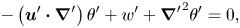 \begin{gather}-\left(\boldsymbol{u}'\boldsymbol{\cdot}\boldsymbol{\nabla}'\right)\theta'+w'+{\boldsymbol{\nabla}'}^{2}\theta'=0, \nonumber\end{gather}
 \begin{gather}\boldsymbol{\nabla}'\boldsymbol{\cdot}{\boldsymbol{u}}'=0, \end{gather}
where  $\lambda$ is a homotopy parameter. For fixed $Ra=10^{4}$, $Pr=1$ and $\boldsymbol {f}'$, we have tracked the solution from $\lambda =1$ to $0$ using the Newton–Krylov method (figure 8). The connected solution ${S}_{3D}$ is the present 3-D steady solution shown in §§ 3 and 4.
Homotopy from the wall-to-wall optimal transport solution at  $Pe=508$ (from Motoki et al. Reference Motoki, Kawahara and Shimizu2018a) to the present 3-D steady solution for a fixed $Ra=10^{4}$ and $Pr=1$. (a) Nusselt number $Nu$ as a function of the homotopy parameter $\lambda$. The red open circle shows the optimal solution ${S}_{op}$ of the Euler–Lagrange equations for the wall-to-wall optimal transport problem, and the red and blue filled circles represent the 3-D steady solution ${S}_{3D}$ and the 2-D steady solution ${S}_{2D}$ of the Boussinesq equations, respectively. (b–d) Isosurfaces of temperature $T/\Delta T=0.6$ at (b) $\lambda =0$, (c) $\lambda =0.3$ and (d) $\lambda =1.0$. The contours represent the temperature $T$ in the planes $x/H=-{\rm \pi} /4$ and $y/H={\rm \pi} /4$. The numerical computation is carried out on $64^{3}$ grid points.
Appendix B. Dependence of multi-scale steady solution on domain size, Prandtl number and spatial resolution
Figure 9 shows the Nusselt number  $Nu$ compensated by $Ra^{0.31}$ and the Reynolds number $Re$ compensated by $Pr^{-2/3}Ra^{4/9}$ as a function of the Rayleigh number $Ra$ in the 3-D steady solutions for different horizontal period $L$ and Prandtl number $Pr$. The magenta, red and orange symbols represent $L/H=2{\rm \pi} /(k_{c}H)\approx 2.02$, ${\rm \pi} /2\approx 1.57$ and $1$, respectively, for $Pr=1$, where $k_{c}=3.117/H$ is the wavenumber corresponding to the minimal critical Rayleigh number $Ra_{c}=1708$ (Drazin & Reid Reference Drazin and Reid1981). Although there is a variation for small $Ra$, the three solutions show similar $Nu$ at $Ra\gtrsim 10^{6}$. The green symbols represent $L/H={\rm \pi} /2$ for $Pr=7$, and the dependence of $Nu$ on $Pr$ is minor. The dependence of $Nu$ on the domain size and $Pr$ (for $1\lesssim Pr\lesssim 10$) is expected to not be significant at a high $Ra$, since the emergence of the small-scale plume and vortex structures near the walls, which are robustly observed for different values of $L$ and $Pr$ (figures 5, 10, 11 and 12), might be a key ingredient in the vertical heat flux. In contrast, a variation in $Re$ exists; however, all the solutions are comparable at $Ra\sim 10^{7}$. The blue filled and open diamonds in figure 9(a) indicate the 2-D optimised steady solutions for $Pr=1$ and $7$, respectively, obtained by Sondak et al. (Reference Sondak, Smith and Waleffe2015). The 3-D steady solutions can exceed the maximal heat flux in the 2-D steady solutions. Meanwhile, at $Ra\gtrsim 10^{6}$ the present 3-D steady solutions with $1\le L/H \lesssim 2$ exhibit smaller $Nu$ than those of the 2-D optimised steady solutions at the same $Pr$.
$Pr$.
(a) Nusselt number  $Nu$ compensated by $Ra^{0.31}$ and (b) Reynolds number $Re$ compensated by $Pr^{-2/3}Ra^{4/9}$ as a function of the Rayleigh number $Ra$ in the 3-D steady solutions for different horizontal period $L$ and Prandtl number $Pr$. The magenta, red and orange symbols represent $L/H=2{\rm \pi} /3.117$, ${\rm \pi} /2$ and $1$, respectively, for $Pr=1$, and the green symbols represent $L/H={\rm \pi} /2$ for $Pr=7$. The blue filled and open diamonds represent the 2-D optimised steady solutions (Sondak et al. Reference Sondak, Smith and Waleffe2015) for $Pr=1$ and $7$, respectively. The blue dashed line indicates the least square fit in the 2-D steady solutions for $Pr=7$, $Nu-1=0.115Ra^{0.31}$, determined in the range $10^{7}< Ra\le 10^{9}$ (Waleffe et al. Reference Waleffe, Boonkasame and Smith2015). The present solutions have been obtained on grid points of $+$,
$+$,  $(N_{x},N_{y},N_{z})=(64,64,64)$; $\bullet$, $(128,128,128)$; $\times$, $(192,192,128)$; $\circ$, $(256,256,256)$.
The 3-D steady solution in the domain with  $L/H=2{\rm \pi} /3.117\approx 2.02$ for $Pr=1$ at (a) $Ra=10^5$, (b) $Ra=10^6$ and (c) $Ra=10^7$. The yellow and grey objects represent the isosurfaces of $T/\Delta T=0.6$ and (a) $Q/(\kappa ^2/H^4)=1.28\times 10^5$, (b) $Q/(\kappa ^2/H^4)=8\times 10^5$ and (c) $Q/(\kappa ^2/H^4)=8\times 10^7$, respectively. The contours indicate $T$ in the plane $y/H={\rm \pi} /3.117$.
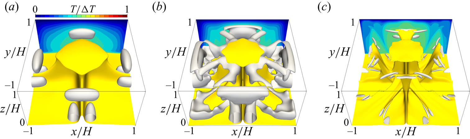
The 3-D steady solution in the domain with  $L/H=1$ for $Pr=1$ at (a) $Ra=10^5$, (b) $Ra=10^6$ and (c) $Ra=10^7$. The yellow and grey objects represent the isosurfaces of $T/\Delta T=0.6$ and (a) $Q/(\kappa ^2/H^4)=1.28\times 10^5$, (b) $Q/(\kappa ^2/H^4)=2.4\times 10^6$ and (c) $Q/(\kappa ^2/H^4)=5\times 10^7$, respectively. The contours indicate $T$ in the plane $y/H=0.5$.
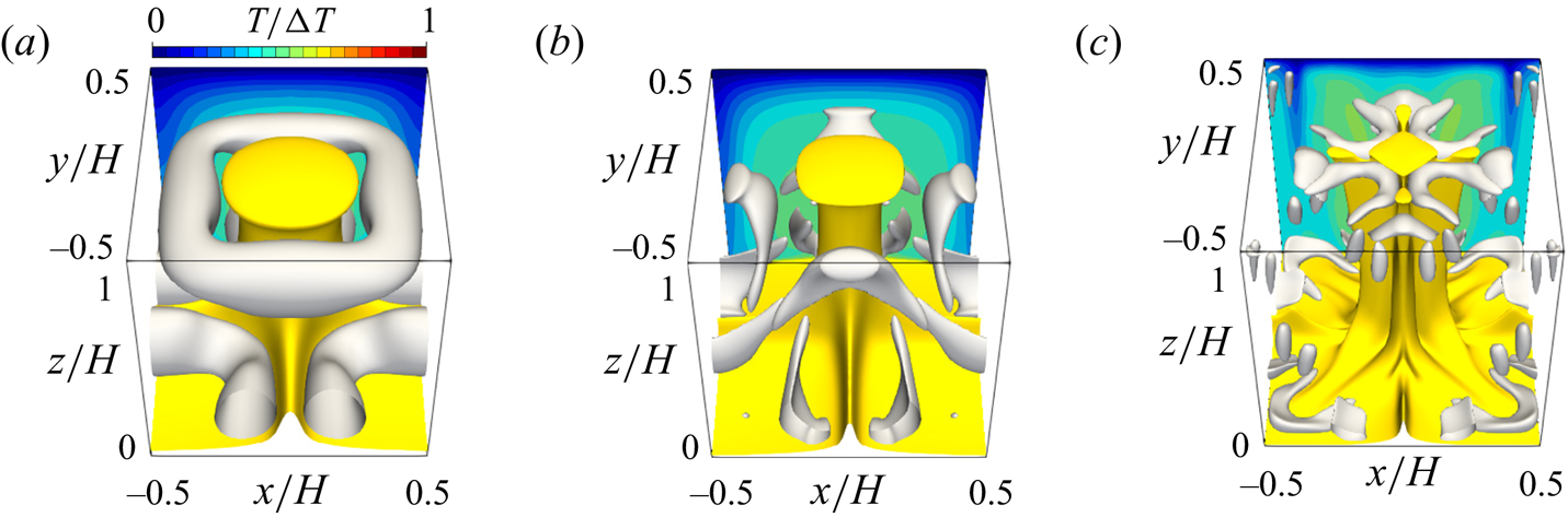
The 3-D steady solution in the domain with  $L/H={\rm \pi} /2\approx 1.57$ for $Pr=7$ at (a) $Ra=10^5$, (b) $Ra=10^6$ and (c) $Ra=10^7$. The yellow and grey objects represent the isosurfaces of $T/\Delta T=0.6$ and (a) $Q/(\kappa ^2/H^4)=1\times 10^5$, (b) $Q/(\kappa ^2/H^4)=1\times 10^6$ and (c) $Q/(\kappa ^2/H^4)=1.28\times 10^7$, respectively. The contours indicate $T$ in the plane $y/H={\rm \pi} /2$.
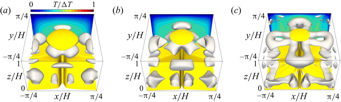
In figure 9 the symbols  $+$,
$+$,  $\bullet$, $\times$ and $\circ$ show the results obtained on different grid points $(N_{x},N_{y},N_{z})=(64,64,64)$, $(128,128,128)$, $(192,192,128)$ and $(256,256,256)$, respectively, and the effects of the spatial resolutions on $Nu$ and $Re$ are minor. For our main results with $L/H={\rm \pi} /2$ and $Pr=1$, the grid points $(N_{x},N_{y},N_{z})=(128,128,128)$ are enough to evaluate the characteristics of the 3-D steady solution at $Ra\lesssim 10^{7}$; $(N_{x},N_{y},N_{z})=(256,256,256)$ are sufficient at $Ra\sim 10^{7}$. Furthermore, the Kolmogorov micro-scale length $\eta$ and the thermal conduction layer thickness $\delta$ in the 3-D steady solution and the turbulent states at $Ra=10^{5},10^{6},10^{7}$ and $10^{7.42}\approx 2.6\times 10^{7}$ are summarised in table 1 together with the grid sizes. Since the energy dissipation rate is a function of the wall-normal coordinate $z$,
$z$,  $\varepsilon (z)=(\nu /2){\langle {(\partial u_{i}/\partial x_{j}+\partial u_{j}/\partial x_{i})}^{2} \rangle }_{xyt}$, $\eta$ also depends on $z$. Here ${\langle \eta \rangle }_{z}$ and $\eta |_{c}$ are based on the total energy dissipation rate, ${\langle \varepsilon \rangle }_{z}$, and that at the centre of the fluid layer, $\varepsilon |_{z=H/2}$, respectively, and ${\langle \eta \rangle }_{z}<\eta |_{c}$ in all cases. The grid size in the $x$ direction, $\Delta x(=\Delta y)$, and the maximal value of $z$,
$z$,  $\Delta z$, are comparable with $\eta$ and less than one-third of $\delta$. Therefore, the spatial resolution is sufficient to resolve the smallest-scale thermal and flow structures in the 3-D steady solution and the turbulent states. The present turbulent direct numerical simulation data are obtained by averaging time of more than 200 convective time units based on the buoyancy-induced terminal velocity $U={(g\alpha \Delta TH)}^{1/2}$.
Numerical details of the 3-D steady solution and the turbulent states for  $L/H={\rm \pi} /2$ and $Pr=1$. Here $\Delta x$ and $\Delta z$ are the spatial resolutions in the $x$ and $z$ directions; ${\langle \eta \rangle }_{z}$ and $\eta |_{c}$ represent the Kolmogorov micro-scale length $\eta ={(\nu ^{3}/\varepsilon )}^{1/4}$ based on the vertical averaged energy dissipation rate, ${\langle \varepsilon \rangle }_{z}=(\nu /2){\langle {(\partial u_{i}/\partial x_{j}+\partial u_{j}/\partial x_{i})}^{2} \rangle }_{xyzt}$, and that at the centre of the fluid layer, $\varepsilon |_{z=H/2}$, respectively; $\delta$ is the thermal conduction layer thickness, $\delta /H=1/(2Nu)$; $\tau$ is the integral time to obtain the statistics; and $U={(g\alpha \Delta T H)}^{1/2}$ is the buoyancy-induced terminal velocity.


 Open access