Quantifying Heterochrony

A novel approach for quantifying heterochrony is proposed herein, whereby a character matrix comprising a series of multistate characters coded for each species within the analysis is developed. Each character represents an aspect of morphology that may exhibit a paedomorphic, peramorphic, or neutral heterochronic expression. The peramorphic and paedomorphic conditions for each character are determined based on a ranked series of criteria:

1. 1. direct observations of ontogenetic changes within the target species;

2. 2. ontogenetic changes observed in closely related species;

3. 3. ontogenetic changes observed in extant relatives;

4. 4. comparison with outgroup juvenile morphology or ontogeny for character polarity; and

5. 5. comparison with outgroup adult morphology for character polarity.

Once the polarity of the morphology of heterochronic expression for each character is established, characters are coded for each species and assigned a score. A paedomorphic condition is assigned a negative (−1) score, a peramorphic condition is assigned a positive (+1) score, and a neutral condition is assigned a score of 0. If a character cannot be coded for a given species, either due to it not being preserved or its condition being otherwise unclear, it is not given a score and does not contribute to the analysis. The total number of characters within the matrix depends on the number of identifiable heterochronically influenced traits within a lineage; as such, organisms with more complex morphologies and better-understood ontogenies will result in larger heterochronic matrices. A larger matrix allows for increased granularity in the heterochronic weighting, and ideally a matrix will comprise 10 or more characters; however, it is possible to generate a heterochronic weighting for a taxon that has as few as three characters coded.

Each of the characters coded for a species in the matrix contributes to the heterochronic weighting of the species, calculated as:

(1)$$Hw_j = \displaystyle{{\mathop \sum \nolimits_{i = 1}^n \eta _i} \over n}$$

where Hw is the heterochronic weighting of species j, derived from the mean of the combined heterochronic scores (η) of n characters, resulting in a value between 1.00 (more peramorphic) and −1.00 (more paedomorphic). In turn, the heterochronic weighting of a given clade is calculated as:

(2)$$\left[ {Hw} \right]_k \,= \,\displaystyle{{\mathop \sum \nolimits_{\,j = 1}^N Hw_j} \over N} $$

where [Hw] is the heterochronic weighting of clade k, derived from the mean of the combined heterochronic weightings (Hw) in N species, again resulting in a value between 1.00 and −1.00. The heterochronic weighting of a clade therefore represents the average of the heterochronic weightings of its constituent species; it is explicitly not an ancestral state reconstruction. What heterochronic weighting does ensure is that all taxa within an analysis have a directly comparable metric, permitting analysis of heterochronic trends and correlation with other evolutionary phenomena. While the scale of the heterochrony metric raw values within an analysis is relative and cannot be directly compared between analyses, patterns and timing of heterochronic shifts can be directly compared between datasets in an identical manner to quantitative analyses of morphospace (Korn et al. Reference Korn, Hopkins and Walton2013; Hopkins and Gerber Reference Hopkins, Gerber, de la Rosa and Müller2017).

To determine whether the heterochronic weighting of a clade represents a concerted trend shift distinct from what could be expected from random, nondirectional evolution, the observed clade scores are randomized across the tree topology. In total, 100,000 randomizations are performed, with the distribution of the randomized heterochronic weightings then collated into a histogram for each clade to which the observed clade heterochronic weighting can be directly compared. If the actual weighting score falls within either tail of the distribution, the weighting is significantly different from what would be expected under random (nondirectional) character change. Randomizing the heterochronic weightings across the observed phylogeny accounts for vagaries such as clade size and topological relationships that may impact the distribution of heterochronic weighting scores. The heterochronic weights retrieved for a given clade are therefore compared with a distribution of weight scores over an identical topology; as such, randomized distributions should be generated for each topology used in an analysis. In this way, disparate analyses can determine whether clades fall within the tails of the expected heterochronic weighting distribution given their phylogenetic topology.

Node- versus Tip-based Analyses

Scores for heterochronic weighting can be applied two ways, through either a node-based or a tip-based analysis (Fig. 1). Applying heterochronic weighting through node-based calculations accurately encompasses the fact that whether a condition for a given taxon is peramorphic, paedomorphic, or neutral is dependent on the condition in its ancestor as inferred by ancestral state reconstruction, and so it is possible for the polarity of a character to change over the evolutionary history of a clade. As such, when applying node-based calculations, it is critical to document the polarity of each character for each node in the phylogeny. Heterochronic weights are calculated for nodes and are reset at the base of each branch of the phylogeny, with individual character weights representing the inferred shift or transition from the ancestral condition. Node-based application of heterochronic weighting more accurately reflects the actual process of heterochrony; however, it is sensitive to sampling, as failing to sample a species can result in an incorrect assumption of character polarity for a given node, while large gaps in sampling can result in unnatural stacking of transitions at sampled nodes. The analysis also becomes incredibly sensitive to phylogenetic topology, as the relative order in which nodes occur will have a major impact on character polarity. Therefore, node-based heterochronic weighting ideally requires a well-constrained and dated phylogeny for an evenly sampled group with good ontogenetic data. In practice, only a minority of clades may combine all of these attributes, limiting the extent to which heterochronic weighting can be applied from a node-based perspective—although the promise of phylogenetic advances in a variety of molluscan groups such as ammonoids and gastropods, which regularly preserve details of their ontogeny and have a good fossil record, marks them as potential candidates for node-based heterochronic weighting.

Figure 1.

Example of heterochronic weightings calculated from three traits evolving across a lineage comprising taxa A–G. In the top tree, evolution of the three traits is shown with their condition (peramorphic + 1, paedomorphic −1, or neutral 0) for each species and internal node of the phylogeny shown in boxes. Transitions between character states are shown beneath each branch. The polarity of a transition is dependent on the condition of the character at the preceding node; therefore, a transition to 0 from −1 would be positive (a peramorphic transition), while a transition to 0 from + 1 would be negative (a paedomorphic transition). Node-based calculations are shown on the bottom left, where heterochronic weights are derived from the transitions leading to each node or tip species, while tip-based calculations of heterochronic weights derived from the terminal character conditions of tip species are shown on the bottom right. Both analytical variations accurately capture the overall peramorphic trend among species A and B and the paedomorphic trend from species E to G. Notably, the tip-based application of the method fails to recognize the peramorphic reversal in species F; however, tip-based heterochronic weights would recognize the peramorphic influence if this were to develop into a long-term trend. Node- and tip-based calculations of heterochronic weights are therefore both equally accurate with regard to recognizing overall trends, but node-based calculations are more precise.

Alternatively, the tip-based application of heterochronic weighting provides a grand average of heterochronic traits within observed taxa compared with the root character polarity. Rather than tracing the transition of the heterochronic event, tip-based heterochronic weighting quantifies the overall outcome of heterochronic events. This makes the method less precise than its node-based articulation, as it may fail to recognize relative polarity changes in characteristics, but is more broadly applicable to groups with uneven sampling or uncertain phylogenetic topology. Tip-based heterochronic weighting gives an overall indication of peramorphic or paedomorphic trends over the evolutionary history of a clade; in this way, it is similar to the method recently used by Martynov et al. (Reference Martynov, Lundin, Picton, Fletcher, Malmberg and Korshunova2020) to study paedomorphosis in nudibranchs, with the distinction that heterochronic weighting provides a quantitative rather than qualitative assessment of the degree of peramorphic or paedomorphic traits within a species. For the present study, heterochronic weighting was applied using the tip-based procedure, as sampling of Xiphosura is uneven across their evolutionary history, as demonstrated by the lack of Silurian exemplars. This is considered an appropriate field test of the method, as I suspect that tip-based analyses will form the bulk of any subsequent studies that adopt heterochronic weighting.

Heterochronic Character Matrix

A heterochronic character matrix for Xiphosura was assembled comprising 20 characters. Characters and their peramorphic and paedomorphic conditions were developed following the criteria detailed in “Quantifying Heterochrony”. The characters encompass a wide variety of xiphosuran morphology, equally divided between traits of the prosoma (anterior tagma) and traits of the thoracetron (posterior tagma) (Figs. 2, 3, Table 1). The resulting matrix, coded for 54 xiphosurid taxa, is available in the Supplementary Material. While a number of aspects of these characters also appear in the phylogenetic character matrix, several (such as body size) are not considered appropriate phylogenetic characters and are not incorporated into the phylogenetic analysis. Those heterochronic characters that are included comprise only a minority (5%) of the total phylogenetic characters, ensuring a degree of independence between the two character sets.

Figure 2.

Heterochronic characters coded for Xiphosura encompassing aspects of overall body size and prosomal morphology, showing paedomorphic (−1), neutral (0), and peramorphic (+1) conditions. A character unavailable for coding in a species is considered missing data (?) and does not contribute to the species score.

Figure 3.

Heterochronic characters coded for Xiphosura encompassing aspects of thoracetron and telson morphology, showing paedomorphic (−1), neutral (0), and peramorphic (+1) conditions. A character unavailable for coding in a species is considered missing data (?) and does not contribute to the species score.

Table 1.

Character traits used in the heterochronic character matrix, detailing the ancestral or base condition and the peramorphic and paedomorphic expression of each. Diagrammatic representations of each character are shown in Figs. 2 and 3.

Determination of polarity of character morphs for assigning peramorphic and paedomorphic conditions was performed with reference to the observed ontogenetic trajectories of extinct and extant species. The most extensive work on xiphosurid development and ontogeny has focused on the extant American species Limulus polyphemus, with studies of embryonic (Scholl Reference Scholl1977; Sekiguchi et al. Reference Sekiguchi, Yamamichi, Costlow, Bonaventura, Bonaventura and Tesh1982; Sekiguchi Reference Sekiguchi and Sekiguchi1988; Shuster and Sekiguchi Reference Shuster, Sekiguchi, Shuster, Barlow and Brockmann2003; Haug and Rötzer Reference Haug and Rötzer2018a) and postembryonic (Sekiguchi et al. Reference Sekiguchi, Seshimo, Sugita and Sekiguchi1988a,Reference Sekiguchi, Seshimo and Sugitab; Shuster and Sekiguchi Reference Shuster, Sekiguchi, Shuster, Barlow and Brockmann2003) ontogeny supplemented by detailed studies of the early development of the thoracic opercula and book gills (Farley Reference Farley2010) and compound lateral eyes (Harzsch et al. Reference Harzsch, Vilpoux, Blackburn, Platchetzki, Brown, Melzer, Kempler and Battelle2006). Comparatively few studies of the extant Asian species’ ontogenies exist; those few that do focus on Tachypleus tridentatus (Sekiguchi et al. Reference Sekiguchi, Yamamichi, Costlow, Bonaventura, Bonaventura and Tesh1982, Reference Sekiguchi, Seshimo, Sugita and Sekiguchi1988a,Reference Sekiguchi, Seshimo and Sugitab; Sekiguchi Reference Sekiguchi and Sekiguchi1988), often via direct comparison with the development of Limulus.

Ontogenetic data also exist for a number of extinct taxa from across the xiphosurid phylogeny. The bellinurines Euproops danae and Euproops sp., from the Carboniferous of the United States and Germany, respectively, have been subject to detailed study of their postlarval development (Schultka Reference Schultka2000; Haug et al. Reference Haug, Van Roy, Leipner, Funch, Rudkin, Schöllmann and Haug2012; Haug and Rötzer Reference Haug and Rötzer2018b; Tashman et al. Reference Tashman, Feldmann and Schweitzer2019). Ontogenetic data have also been reported from the bellinurine Alanops magnificus, known from the Carboniferous Montceau-les-Mines Konservat-Lagerstätte in France, a species considered to demonstrate a paedomorphically derived adult morphology (Racheboeuf et al. Reference Racheboeuf, Vannier and Anderson2002). Bellinurine embryonic larvae preserved within egg clutches have also been reported from the Carboniferous of Russia and assigned to the newly erected species Xiphosuroides khakassicus (Shpinev and Vasilenko Reference Shpinev and Vasilenko2018), which probably represent the larvae of an existing species of Bellinurus. Outside of the bellinurines, juvenile and adult individuals of the paleolimulid Paleolimulus kunguricus, from the Permian of Russia have been described (Naugolnykh Reference Naugolnykh2017). Subadult and adult stages have also been differentiated among the available material of the Cretaceous tachypleine Tachypleus syriacus from the Hâqel and Hjoûla Konservat-Lagerstätten of Lebanon (Lamsdell and McKenzie Reference Lamsdell and McKenzie2015), while the Cretaceous mesolimulid Mesolimulus tafraoutensis from the Gara Sbaa Konservat-Lagerstätte of Morocco is known from juvenile material (Lamsdell et al. Reference Lamsdell, Tashman, Pasini and Garassino2020).

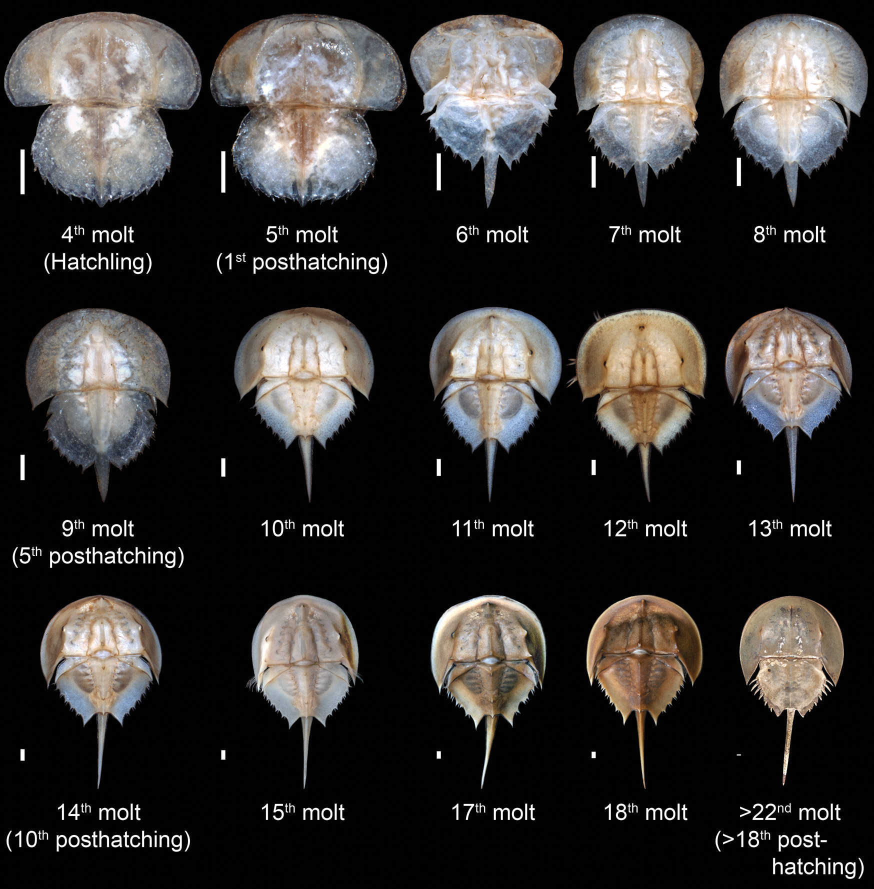
This diversity in phylogenetic sampling of xiphosurid ontogeny reveals a number of consistent trends in horseshoe crab development across their evolutionary history that can still be observed in the ontogeny of modern species (Fig. 4). These evolutionarily conserved ontogenetic trends include a progressive reduction in expression of the prosomal ophthalmic ridge from the larval form through to the adult, a relative decrease in the length of the prosomal appendages, a reduction in expression of the free lobe segment, an increase in the number and complexity of opisthosomal opercula, and an increase in the relative length of the telson compared with the body. It is these traits, alongside other observed consistent trends in xiphosuran ontogeny, that were incorporated into the heterochronic character matrix.

Figure 4.

Ontogenetic sequence of Limulus polyphemus from the Yale Peabody Museum teaching collection, beginning with the hatchling (fourth molt) and proceeding to the adult (post–22^nd molt, which corresponds to the 18^th posthatching molt). The final molt is represented by specimen YPM IZ 070174. The size of each instar has been standardized to more clearly demonstrate changes in relative morphological proportions. Scale bars, 1 mm.

Phylogenetic Analysis

A phylogenetic framework for Xiphosura was constructed using an expanded version of the chelicerate character matrix from Lamsdell (Reference Lamsdell2016), which itself draws on matrices presented in Lamsdell (Reference Korn, Hopkins and Walton2013), Selden et al. (Reference Selden, Lamsdell and Liu2015), Lamsdell and McKenzie (Reference Lamsdell and McKenzie2015), and Lamsdell et al. (Reference Lamsdell, Briggs, Liu, Witzke and McKay2015). The resulting matrix comprises 256 characters coded for 153 taxa and is available in the online MorphoBank database (O'Leary and Kaufman Reference O'Leary and Kaufman2012) under the project code p2606 (accessible from http://morphobank.org/permalink/?P2606) as well as in the Supplementary Material. Sampling of Xiphosurida within the matrix was increased by six, incorporating Limulus woodwardi (Watson Reference Watson1909) and the newly described Limulitella tejraensis (Błażejowski et al. Reference Błażejowski, Niedźwiedzki, Boukhalfa and Soussi2017), M. tafraoutensis (Lamsdell et al. Reference Lamsdell, Tashman, Pasini and Garassino2020), P. kunguricus (Naugolnykh Reference Naugolnykh2017), Paleolimulus woodae (Lerner et al. Reference Lerner, Lucas and Mansky2016), and Vaderlimulus tricki (Lerner et al. Reference Lerner, Lucas and Lockley2017). Three taxa were removed from the matrix: Anacontium brevis, which is a synonym of the co-occurring Anacontium carpenteri (Anderson Reference Anderson1997); Liomesaspis leonardensis, which is poorly preserved and lacks diagnostic characters separating it from Liomesaspis laevis (see Tasch Reference Tasch1961); and Willwerathia laticeps, which may not be a chelicerate (Lamsdell Reference Lamsdell2019). In total, 54 Xiphosura (sensu Lamsdell Reference Lamsdell2013, Reference Lamsdell2016) were included, and it is these taxa that were the focus of subsequent analyses of heterochrony and ecological affinity, with the remaining 99 taxa within the matrix serving to adequately root and demonstrate the monophyly of the xiphosuran clade. Additionally, the character coding for Yunnanolimulus luopingensis was updated to incorporate information from recently described specimens exhibiting exceptional preservation (Hu et al. Reference Hu, Zhang, Feldmann, Benton, Schweitzer, Wen, Zhou, Xie, Lü and Hong2017). Four new characters were also added to the matrix, encompassing cardiac lobe width (character 32), the cardiac lobe bearing a median cardiac ridge with rounded cross section (character 38), the occurrence of a genal groove (character 45), and the course and extent of the genal groove (character 46). Morphological terminology for character definitions follows Selden and Siveter (Reference Selden and Siveter1987) and Lamsdell (Reference Lamsdell2013).

Tree inference was performed using Bayesian statistical analysis, which has been shown to outperform maximum parsimony analyses of simulated data (Wright and Hillis Reference Wright and Hillis2014; O'Reilly et al. Reference O'Reilly, Puttick, Parry, Tanner, Tarver, Fleming, Pisani and Donoghue2016; Puttick et al. Reference Puttick, O'Reilly, Tanner, Fleming, Clark, Holloway, Lozano-Fernandez, Parry, Tarver, Pisani and Donoghue2017, Reference Puttick, O'Reilly, Pisani and Donoghue2019), although tree topologies derived from empirical data analyzed under parsimony methods exhibit higher stratigraphic congruence than those retrieved from Bayesian analysis (Sansom et al. Reference Sansom, Choate, Keating and Randle2018). Bayesian inference was performed using Markov chain Monte Carlo analyses as implemented in MrBayes 3.2.6 (Huelsenbeck and Ronquist Reference Huelsenbeck and Ronquist2001), with four independent runs of 100,000,000 generations and four chains each under the maximum-likelihood model for discrete morphological character data (Mkv + Γ; Lewis Reference Lewis2001), with gamma-distributed rate variation among sites. All characters were treated as unordered and equally weighted (Congreve and Lamsdell Reference Congreve and Lamsdell2016). Trees were sampled with a frequency of every 100 generations, resulting in 1,000,000 trees per run. The first 25,000,000 generations (250,000 sampled trees) of each run were discarded as burn-in, and the 50% majority rule consensus tree was calculated from the remaining 750,000 sampled trees across all four runs; this represents the optimal summary of phylogenetic relationships given the available data (Holder et al. Reference Holder, Sukumaran and Lewis2008). Posterior probabilities were calculated from the frequency at which a clade occurred among the sampled trees included in the consensus tree.

Additionally, maximum parsimony analysis was performed using TNT (Goloboff et al. Reference Goloboff, Farris and Nixon2008) (made available with the sponsorship of the Willi Hennig Society) to test for topological congruence between Bayesian and parsimony methods. The search strategy employed 100,000 random addition sequences with all characters unordered and of equal weight (Congreve and Lamsdell Reference Congreve and Lamsdell2016), each followed by tree bisection-reconnection branch swapping (the mult command in TNT). Jackknife (Farris et al. Reference Farris, Albert, Källersjö, Lipscomb and Kluge1996), bootstrap (Felsenstein Reference Felsenstein1985), and Bremer (Bremer Reference Bremer1994) support values were also calculated in TNT and the ensemble Consistency, Retention and Rescaled Consistency Indices were calculated in Mesquite 3.02 (Maddison and Maddison Reference Maddison and Maddison2018). Bootstrapping was performed with 50% resampling for 1,000 repetitions, while jackknifing was performed using simple addition sequence and tree bisection-reconnection branch swapping for 1,000 repetitions with 33% character deletion.

Ecological Affinity

Previous work by Kiessling and Aberhan (Reference Kiessling and Aberhan2007) and Hopkins (Reference Hopkins2014) has set out a series of standard environmental categories for organisms found in marine environments; latitudinal occupation, substrate preference, bathymetry, and reef association. For the present study, however, a novel characteristic is considered: salinity. Previous work has shown that horseshoe crabs invaded nonmarine environments multiple times over their evolutionary history (Lamsdell Reference Lamsdell2016), a transition associated with a variety of biomechanical and physiological challenges (Lamsdell Reference Lamsdellin press), and it is these macroevolutionary events that comprise the focus of the work herein. As with the characteristics of Kiessling and Aberhan (Reference Kiessling and Aberhan2007) and Hopkins (Reference Hopkins2014), salinity is reduced to a binary variable, and species are assigned either a marine or nonmarine (including freshwater and deltaic/transitional marginal-marine environments with a large amount of continental flora and fauna) affinity. The ecological affinity for each taxon was estimated through the modified method of Miller and Connolly (Reference Miller and Connolly2001). This is a departure from Hopkins (Reference Hopkins2014), who implemented a refined version of the Bayesian estimation of affinity developed by Simpson and Harnik (Reference Simpson and Harnik2009), which has traditionally been applied to higher taxa (e.g., genera). The drawback of applying the Bayesian estimation method to species data is that it requires multiple samples; Simpson and Harnik (Reference Simpson and Harnik2009) only considered genera with at least four occurrences. This is impossible for many species in the fossil record, particularly unmineralized marine organisms (which include horseshoe crabs), the majority of which are known solely from single localities—representing only a single occurrence. In contrast, the method of Miller and Connolly (Reference Miller and Connolly2001) simply calculates the affinity of a taxon for a given environment as the number of occurrences within the environment divided by the total number of occurrences, resulting in a metric ranging from 0 to 1; when combined, the value of the metric for each of the two possible affinities and no clear affinity will always sum to 1. The advantage of this method is that it can operate with only a single observation, with the drawback that lower sample sizes increase the chances of a false positive of ecological affinity. However, species tend to have a narrow range of habitat preferences (Saupe et al. Reference Saupe, Hendricks, Portell, Dowsett, Haywood, Hunter and Lieberman2014, Reference Saupe, Qiao, Hendricks, Portell, Hunter, Soberón and Lieberman2015), thereby reducing the chance of occurrences outside their preferred environments; when species do have broader habitat preferences, they also tend to have broader geographic ranges, increasing the probability of fossilization and thereby increasing the available sample size, reducing the chance of false positives.

The resulting metrics for ecological affinity were interpreted as any single value >0.5 indicating a preference for that environment. When no single environment scored >0.5, the taxon was considered to exhibit no affinity. Ties (an instance where the highest-scoring environment achieved a 0.5) were also considered an indication of no affinity. In practice, as the majority of horseshoe crab species are known from only one or a handful of localities, most species showed a clear ecological affinity (see Supplementary Material).

Phylogenetic Paleoecology

The emergent field of phylogenetic paleoecology leverages phylogenetic information to assess the long-term evolutionary significance of ecological trends within lineages through the synthesis of phylogenetic theory and quantitative paleoecology (Lamsdell et al. Reference Lamsdell, Congreve, Hopkins, Krug and Patzkowsky2017). Using the historical phylogenetic and ecological framework, it is possible to test for phylogenetic or ecological signal in the distribution of heterochronic weightings, thereby accounting for the possible influence of both the genealogical and ecological biological hierarchies (Congreve et al. Reference Congreve, Falk and Lamsdell2018).

The phylogenetic framework also permits for the estimation of the ancestral conditions of both morphological and ecological characteristics. To determine the number of transitions between marine and nonmarine environments, the ecological affinity of each species as determined above was mapped onto the resulting phylogenetic tree and parsimony-based ancestral state reconstruction performed in Mesquite 3.02 (Maddison and Maddison Reference Maddison and Maddison2018). The inferred ancestral ecological affinities were used to polarize the internal nodes of the tree, thereby establishing whether the ecological affinities of tip species represent inherited habitat preferences or are the result of a shift in the occupied niche.

Multivariate statistical tests (permutational multivariate analysis of variance [PERMANOVA] using the Euclidian distance measure) were performed in the statistical software package PAST (Hammer et al. Reference Hammer, Harper and Ryan2001) and using the adonis function in the R (R Core Team 2018) package vegan (Oksanen et al. Reference Oksanen, Blanchet, Friendly, Kindt, Legendre, McGlinn, Michin, O'Hara, Simpson, Solymos, Stevens, Szoecs and Wagner2019) to ascertain the statistical significance of differences in heterochronic weightings across ecological affinities and phylogenetic clades. Several analyses were performed: comparison between marine and nonmarine habitats, comparison between clades, and a test of the interaction between clade and habitat categories. For the comparison between marine and nonmarine habitats, all species were included in the analysis. However, for analyses that required the assignment of species to clades, only species assignable to Bellinurina, Paleolimulidae, Austrolimulidae, or Limulidae were included. This resulted in the exclusion of Lunataspis aurora and Kasibelinurus amoricum (stem Xiphosurida), Bellinuroopsis rossicus and Rolfeia fouldenensis (stem Limulina), and Valloisella lievinensis (stem Limulidae), as their inclusion would necessitate the formulation of unnatural, paraphyletic “groups” that possess no evolutionary cohesion and could serve to bias analyses. Significance was estimated by permutation across groups with 10,000 replicates, including Bonferroni correction to correct for multiple comparisons in the case of comparison between clades.

To test whether the distributions of species’ heterochronic weightings within clades exhibit directional trends, Spearman's (Reference Spearman1904) rank correlation coefficient ρ, calculated using the cor.test function in R (R Core Team 2018), was used to compare the heterochronic weighting of observed taxa within a clade to their distance from the root of the clade. A statistically significant ρ, in combination with a statistically significant clade heterochronic weighting [Hw], was considered evidence of a concerted heterochronic trend within the clade. The distance of a species from the root of the clade was determined using the cladistic rank method (Gauthier et al. Reference Gauthier, Kluge and Rowe1988; Norell and Novacek Reference Norell and Novacek1992a,Reference Norell and Novacekb; Norell Reference Norell1993; Benton and Storrs Reference Benton and Storrs1994; Benton and Hitchin Reference Benton and Hitchin1997; Carrano Reference Carrano2000, Reference Carrano, Carrano, Gaudin, Blob and Wible2006; Wagner and Sidor Reference Wagner and Sidor2000; Poulin Reference Poulin2005; Prado and Alberdi Reference Prado and Alberdi2008; Huttenlocker Reference Huttenlocker2014). Cladistic rank is determined by counting the sequence of primary nodes in a cladogram from the basal node to the ultimate node (Fig. 5). The main axis of the cladogram is defined as the internal branch supporting the most inclusive clade after each bifurcation. Smaller offshoot clades are reduced to polytomies for the purpose of assigning a clade rank, with each constituent species within a polytomy receiving the same rank. The assignment of equal rank to all constituents of an offshoot clade is a conservative approach that ensures any revealed trend is the majority pattern demonstrated by the most inclusive clades within the cladogram, without biasing the analysis through exclusion of taxa located in offshoot clades. This was done for each of the four main xiphosurid clades: Bellinurina, Paleolimulidae, Austrolimulidae, and Limulidae.

Figure 5.

Example of the method for assigning taxa to clade ranks for Spearman's rank correlation.