


1. Introduction
The monoclinal flood wave is a travelling waveform that one can often encounter in shallow water flows (Moots & Mavis Reference Moots and Mavis1938; Whitham Reference Whitham1974; Le Méhauté Reference Le Méhauté1976; Ferrick Reference Ferrick2005; Shome & Steffler Reference Shome and Steffler2006; Fowler Reference Fowler2011). In recent years, many research groups have contributed to formulating a hydrodynamic-like framework for describing granular flows. In this context, our group established the theoretical existence of the monoclinal wave in granular chute flow (Razis, Kanellopoulos & van der Weele Reference Razis, Kanellopoulos and van der Weele2018, Reference Razis, Kanellopoulos and van der Weele2019) by employing the appropriately modified granular Saint-Venant equations (Savage & Hutter Reference Savage and Hutter1989; Forterre Reference Forterre2006; Gray & Edwards Reference Gray and Edwards2014; Viroulet et al. Reference Viroulet, Baker, Edwards, Johnson, Gjaltema, Clavel and Gray2017).
A typical monoclinal wave is sketched in figure 1. It may be formed if we allow extra material to flow over a pre-existing thin, uniform sheet of height  $h_{+}$ that propagates with mean velocity $\bar {u}_{+}$. Thus, a sheet of greater height $h_{-}$ and speed $\bar {u}_{-}$ is created on the upstream flank. This waveform retains its stability as long as the Froude number in the upper plateau does not exceed a critical threshold, ${Fr}_{{cr}}$. In the context of one-dimensional flow, the Froude number is defined as follows:
 \begin{equation} {Fr}(x,t)=\frac{\bar{u}(x,t)}{ \sqrt{ h(x,t) g \cos \zeta} } , \end{equation}
where  $\bar {u}(x,t)$ is the depth-averaged velocity of the granular sheet, $h(x,t)$ is its height, $g$ is the gravitational acceleration and $\zeta$ is the inclination angle of the chute.
Granular monoclinal flood wave on a chute (Razis et al. Reference Razis, Kanellopoulos and van der Weele2018): a flowing sheet of uniform height  $h_{-}$ and depth-averaged velocity $\bar {u}_{-}$ overtakes a shallower and slower flow of height $h_{+}$ and velocity $\bar {u}_{+}$. The monoclinal wave, being the travelling shock structure connecting these two regions, is stable as long as the Froude number ${Fr}_{-}$ of the upper plateau does not exceed a critical value ${Fr}_{{cr}}$ given by (3.18). It propagates at a wave speed $c$ exceeding the velocities of the granular materials in both plateaus, i.e. $c > \bar {u}_{-} > \bar {u}_{+}$.

The paper is organized as follows. In § 2 the governing equations, being the one-dimensional Saint-Venant equations adapted to the granular context, are introduced. We then give the fundamental solution representing the stable uniform flow. In § 3 the dynamical system that governs all possible wave solutions (travelling and standing) is derived, its fixed points are located and their local stability properties are determined. Then, in this context, the critical Froude number for the fundamental solution (stable uniform flow) is found. In § 4 the geometrical shape of the orbit of the granular monoclinal wave in phase space is determined. Based on the above findings, and on the form of the first-order approximation of the granular Saint-Venant equations, a classification of the monoclinal waveform is given. Finally, in § 5 the paper is concluded with a recapitulation of the main results and with a computational experiment confirming the stability of the granular monoclinal waves.
2. The Saint-Venant equations for granular chute flow
The dynamics of a flowing granular sheet, in analogy with the shallow water approximation in normal fluids, is described in terms of its height  $h(x,t)$ and depth-averaged velocity $\bar {u}(x,t)$. The latter is defined as $\bar {u}(x,t) = h(x,t)^{-1}\int _{0}^{h(x,t)} u(x,z,t) \,\textrm {d}z$, where $u(x,z,t)$ is the detailed velocity profile depending on the depth $z$. Flow variations in the crosswise direction are ignored; hence both $h(x,t)$ and $\bar {u}(x,t)$ depend only on $x$ and $t$ (cf. figure 1). Furthermore, it is assumed that the granular sheet has a constant density, so it is treated as an incompressible fluid (Savage & Hutter Reference Savage and Hutter1989).
The height  $h(x,t)$ and the depth-averaged velocity $\bar {u}(x,t)$ are governed by a system of two coupled, nonlinear partial differential equations (PDEs) (Gray & Edwards Reference Gray and Edwards2014; Razis et al. Reference Razis, Edwards, Gray and van der Weele2014; Edwards & Gray Reference Edwards and Gray2015; Razis et al. Reference Razis, Kanellopoulos and van der Weele2018; Edwards et al. Reference Edwards, Russell, Johnson and Gray2019; Razis et al. Reference Razis, Kanellopoulos and van der Weele2019), namely the mass conservation
 \begin{equation} \frac{\partial h}{\partial t} + \frac{\partial}{\partial x} (h \bar{u}) = 0 \end{equation}
and the momentum balance
 \begin{align} \frac{\partial}{\partial t} (h \bar{u}) + \frac{\partial}{\partial x} (h \bar{u}^{2}) = gh\sin\zeta - \frac{\partial}{\partial x}\left(\frac{1}{2}gh^{2}\cos\zeta\right) - \mu(h, \bar{u})gh \cos\zeta + \frac{\partial}{\partial x}\left(\nu h^{3/2}\frac{\partial \bar{u}}{\partial x}\right). \end{align}
The terms on the right-hand side of (2.2) represent the following.
(i) The gravity component along the $x$ direction, with $g=9.81\ \textrm {m}\ \textrm {s}^{-2}$.
(ii) The force arising from variations in
$h(x,t)$, i.e. the negative gradient of the depth-averaged pressure.(iii) The frictional force exerted by the chute bed, modelled as a (height- and velocity-dependent) friction coefficient
$\mu (h,\bar {u})$ multiplied by the normal reaction force acting on the granular sheet.


For the friction coefficient, the modified expression for the fully dynamic regime introduced by Edwards et al. (Reference Edwards, Viroulet, Kokelaar and Gray2017) is adopted:
 \begin{equation} \mu(h,\bar{u}) = \tan \zeta_1 + (\tan \zeta_2 - \tan \zeta_1)\left(1 + \frac{\beta h}{\mathcal{L} ({Fr}+\varGamma)}\right)^{{-}1}. \end{equation}
Here  $\zeta _1$, $\zeta _2$, $\mathcal {L}$, $\beta$ and $\varGamma$ are experimental parameters. The angles $\zeta _{1}$ and $\zeta _{2}$ denote the two inclination angles that delimit the interval in which uniform granular flows are possible. For $\zeta < \zeta _{1}$ the granular sheet remains at rest, whereas for $\zeta > \zeta _{2}$ it flows downwards in an accelerated fashion. The parameter $\mathcal {L}$ has its origins in the functional form of the experimental fit concerning the critical angle curves that determine the friction force (Pouliquen & Forterre Reference Pouliquen and Forterre2002). It represents a characteristic thickness (usually ranging from $1$ to $2$ particle diameters) of flow over which a transition between the angles $\zeta _{1}$ and $\zeta _{2}$ occurs in the friction law (2.3). Its exact value depends both on the properties of the grains and on the bed roughness (Pouliquen & Forterre Reference Pouliquen and Forterre2002; Edwards et al. Reference Edwards, Viroulet, Kokelaar and Gray2017). The parameter $\beta$ and the Froude number offset $\varGamma$ are closely related (Forterre & Pouliquen Reference Forterre and Pouliquen2003):
 \begin{equation} {Fr} = \beta \frac{h}{h_{{stop}}(\zeta)}-\varGamma, \end{equation}
where  $h_{{stop}}(\zeta )$ denotes the thickness of the deposition layer that is left on the chute, at an inclination angle $\zeta$, after a uniform flow has passed over it. A first version of (2.4) (without the $\varGamma$ offset) was derived by Pouliquen (Reference Pouliquen1999) by experimentally measuring the Froude number as a function of the quotient $h/h_{{stop}}$ for four different systems of glass beads, revealing their linear relation which is independent of the bead size, the inclination and the roughness condition. The Froude offset $\varGamma$ was introduced by Forterre & Pouliquen (Reference Forterre and Pouliquen2003) in order to fit the experimental results concerning the mean velocity for different materials (sand and glass) into a single law, thus formulating (2.4). In this context we note that the factor $1/\sqrt {\cos \zeta }$ was absent from their definition of the Froude number ${Fr}$ and the offset $\varGamma$. In Edwards et al. (Reference Edwards, Viroulet, Kokelaar and Gray2017) also the parameter $\beta _{*}$ was introduced, expressing the Froude number value at a height $h=h_{*}(\zeta )$ with $h_{{stop}}(\zeta )< h_{*}(\zeta )< h_{{start}}(\zeta )$. Here $h_{*}(\zeta )$ denotes the level of the thinnest (and therefore slowest) possible steady uniform flow which leaves a deposit of smaller thickness $h_{{stop}}(\zeta )$. In the same spirit, $h_{{start}}(\zeta )$ denotes the height for which a static layer is mobilized when the inclination is increased to an angle $\zeta$. As such, it is guaranteed that the granular chute flow remains fully dynamic as long as $Fr\geqslant \beta _{*}$ (Edwards et al. Reference Edwards, Viroulet, Kokelaar and Gray2017).
(iv) The viscous-like diffusive term arising from depth-averaging the in-plane stresses in the sheet. Here, the analytical expression derived by Gray & Edwards (Reference Gray and Edwards2014) is adopted:
 \begin{equation} \nu = \nu(\zeta) = \frac{2 \mathcal{L} \sqrt{g} \sin\zeta }{9 \beta \sqrt{\cos\zeta}}\,\gamma(\zeta),\quad \textrm{where}\ \gamma(\zeta) = \frac{\tan \zeta_2 - \tan\zeta}{\tan\zeta - \tan \zeta_1}. \end{equation}
The granular monoclinal wave consists of two uniformly moving plateaus linked together via a shock front (Razis et al. Reference Razis, Kanellopoulos and van der Weele2018, Reference Razis, Kanellopoulos and van der Weele2019). The steady uniform flow corresponds to the constant solution of the granular Saint-Venant equations (2.1)–(2.2) when all derivatives with respect to  $x$ and $t$ vanish, leaving only $\tan \zeta = \mu (h,\bar {u})$. This condition expresses the balance between the forces of gravity and friction (Razis et al. Reference Razis, Kanellopoulos and van der Weele2018). Now, we can express the velocity of the uniform plateaus as follows:
 \begin{equation} \bar{u}_\pm{=} \frac{\beta \sqrt{g \cos \zeta}}{\mathcal{L} \gamma(\zeta)}\,h_{{\pm}}^{3/2} - \varGamma \sqrt{g \cos \zeta}~ h_{{\pm}}^{1/2}, \end{equation}
and the corresponding Froude number takes the form
 \begin{equation} {Fr}_\pm{=} {Fr}_{{\pm}}(h_\pm,\bar{u}_\pm) = \frac{\bar{u}_\pm}{\sqrt{g h_\pm \cos \zeta}} = \frac{\beta}{\mathcal{L} \gamma(\zeta)}\,h_{{\pm}}-\varGamma. \end{equation}
The velocity of the shock front is given by the well-known formula (Whitham Reference Whitham1974)
 \begin{equation} c =\frac{h_{-}\bar{u}_{-}-h_{+}\bar{u}_{+}}{h_{-}-h_{+}}, \end{equation}
which reflects the fact that in the steady state, for an observer in the co-moving frame, the flux of material entering the shock structure must be equal to the flux leaving the shock, i.e.  $h_{+}(\bar {u}_{+}-c)=h_{-}(\bar {u}_{-}-c)$. Although in the shock region the inertial terms are not exactly zero, they are sufficiently small to justify this expression which is based on kinematic considerations alone, namely the mass conservation across the shock (Razis et al. Reference Razis, Kanellopoulos and van der Weele2018).
Equation (2.8) with the help of equation (2.6) can be expressed in a form which does not contain the velocities  $\bar {u}_{\pm }$:
 \begin{equation} c = \frac{\beta \sqrt{g \cos \zeta}}{\mathcal{L} \gamma(\zeta)} \left( \frac{h_{-}^{5/2}-h_{+}^{5/2}}{h_{-}-h_{+}} \right) - \varGamma \sqrt{g \cos \zeta}~ \left( \frac{h_{-}^{3/2}-h_{+}^{3/2}}{h_{-}-h_{+}} \right). \end{equation}
From (2.9) one might have the impression that when  $\varGamma >0$, the shock speed decreases. This is not the case; in fact the opposite is true as may be seen by fixing the values of the Froude numbers in both plateaus. Equation (2.7) demonstrates that in the presence of the $\varGamma$ offset, the corresponding heights of the plateaus increase and as a consequence, (2.9) returns a greater shock speed than for $\varGamma =0$. This will become even more evident later, in § 3, when we introduce the non-dimensional equations.
Another aspect that is worth noting here is that the minimum height for the lower plateau, in the fully dynamic regime, can be found by setting  $Fr_{+}=\beta _{*}$ and solving equation (2.7) for $h_{+}$. The resulting expression is
 \begin{equation} h_{+,{min}} = \frac{\mathcal{L} \gamma(\zeta)}{\beta}(\beta_{*}+\varGamma). \end{equation}
 Finally, for completeness, we should note that the advective term  $\partial _x (h \bar {u}^{2})$ in (2.2) may be multiplied by a shape factor to obtain an optimal correspondence with experiments (Saingier, Deboeuf & Lagrée Reference Saingier, Deboeuf and Lagrée2016; Lagrée et al. Reference Lagrée, Saingier, Deboeuf, Staron and Popinet2017). This factor, for a steady flow with a Bagnold velocity profile, is equal to $\alpha =5/4$ (GDR-MiDi 2004; Börzsönyi, Hasley & Ecke Reference Börzsönyi, Hasley and Ecke2005; Gray & Edwards Reference Gray and Edwards2014). However, for shallow granular flows with relatively small Froude number, as in the current paper, the solutions are quite insensitive to the shape factor's value (Saingier et al. Reference Saingier, Deboeuf and Lagrée2016; Viroulet et al. Reference Viroulet, Baker, Edwards, Johnson, Gjaltema, Clavel and Gray2017). In fact, in an experimental study by Forterre (Reference Forterre2006) (see in particular figure 1 in that paper) it was found that the plug flow with shape factor value $\alpha =1$ gave a better correspondence with the experimental data than the Bagnold profile, for which $\alpha$ would be $5/4$.
3. Dynamical systems approach
3.1. Travelling wave solution and stability analysis
The monoclinal wave is a travelling waveform propagating without change of shape and at a constant velocity  $c$. Therefore its height and depth-averaged velocity are of the general form $h(x,t) = h(x-ct) = h(\xi )$ and $\bar {u}(x,t) = \bar {u}(x-ct) = \bar {u}(\xi )$, and consequently the governing equations (2.1)–(2.2) become ordinary differential equations. The mass balance equation (2.1) reduces to
 \begin{equation} -ch + h\bar{u} ={-}K, \end{equation}
where the integration constant  $K$ corresponds to the flux of the material per unit width of the channel in the co-moving frame. Using (2.6), this flux constant can be written as a function of height only:
 \begin{equation} K = h_{{\pm}} (c- \bar{u}_{{\pm}}) = c h_{{\pm}}- \frac{\beta \sqrt{g \cos \zeta}}{\mathcal{L} \gamma(\zeta)}h_{{\pm}}^{5/2} + \varGamma \sqrt{g \cos \zeta} h_{{\pm}}^{3/2}. \end{equation}
Solving (3.1) with respect to  $\bar {u}$, we find the first and the second derivative $\bar {u}_{\xi },\bar {u}_{\xi \xi }$ in terms of $h$, and then we substitute into the momentum balance equation (2.2). This leads to the following second-order ordinary differential equation:
 \begin{equation} \frac{\nu K}{h^{3/2}}h'' - \frac{\nu K}{2 h^{5/2}}(h')^{2} + \left(\frac{K^{2}}{h^{3}}-g\cos\zeta\right)h' + g\sin\zeta - \mu(h)g\cos\zeta = 0, \end{equation}
where now  $\mu (h)$ has the form
 \begin{equation} \mu(h) = \tan \zeta_1 + \frac{\tan \zeta_2 - \tan \zeta_1}{1 + \dfrac{\beta h}{\mathcal{L} \left(\varGamma+\left(c-Kh^{{-}1}\right) \left(gh\cos\zeta\right)^{{-}1/2}\right)}}. \end{equation}
Equation (3.3) governs all the travelling and the standing, when  $c=0$, waveforms for granular chute flow that are sustained by the Saint-Venant equations (2.1)–(2.2).
Here, it is convenient to introduce non-dimensional variables, denoted by a tilde, as follows:  $h = h_{-} \tilde {h}$ and $\xi = h_{-} \tilde {\xi }$ (and also $h_{+} = h_{-} \tilde {h}_{+}$). That is, all length scales are measured in terms of the thickness $h_{-}$ of the incoming flow. With this rescaling, the differential equation (3.3) takes the non-dimensional form
 \begin{equation} \frac{\textrm{d}^{2} \tilde{h}}{\textrm{d} \tilde{\xi}^{2}} - \frac{1}{2 \tilde{h}} \left(\frac{\textrm{d} \tilde{h}}{\textrm{d}\tilde{\xi}} \right)^{2} + \frac{ R \tilde{h}^{3/2} }{ {Fr}_{-}^{2} (\tilde{c}-1) } \left[ \left( \frac{ {Fr}_{-}^{2} (\tilde{c}-1)^{2} }{\tilde{h}^{3}} -1 \right) \frac{\textrm{d} \tilde{h}}{\textrm{d} \tilde{\xi}} + \tan \zeta - \mu(\tilde{h}) \right]=0, \end{equation}
with
 $$\begin{gather} \mu(\tilde{h}) = \tan \zeta_1 + \frac{\tan \zeta_2 - \tan \zeta_1}{1 + \dfrac{\gamma(\zeta)\tilde{h}({Fr}_{-}+\varGamma)}{\varGamma+Fr_{-}(\tilde{c} \tilde{h}-\tilde{c}+1) \tilde{h}^{{-}3/2}}}, \end{gather}$$
 $$\begin{gather}\tilde{c} =\frac{c}{\bar{u}_{-}}= \frac{1}{1-\tilde{h}_{+}}\,\frac{1}{Fr_{-}} \left(({Fr}_{-}+\varGamma)(1-\tilde{h}_{+}^{5/2})-\varGamma(1-\tilde{h}_{+}^{3/2}) \right), \end{gather}$$
and the granular Reynolds number defined by
 \begin{equation} R =\frac{\mathcal{L} \gamma(\zeta) \sqrt{g \cos \zeta}\,({Fr}_{-}+\varGamma)}{\beta \nu(\zeta)}\,{Fr}_{-} . \end{equation}
Equation (3.5) first appeared in a study by Gray & Edwards (Reference Gray and Edwards2014) of granular roll waves and also featured in Razis et al. (Reference Razis, Kanellopoulos and van der Weele2019) in the context of the transition from the granular monoclinal waves to (granular) roll waves. Here, despite the fact that (3.5) is identical, the constitutive relations (3.6), (3.7) and (3.8) are different, due to the inclusion of the  $\varGamma$ offset. Of course, for $\varGamma =0$ one recovers the exact same expressions as in Razis et al. (Reference Razis, Kanellopoulos and van der Weele2019). We also note that the shock speed given by (3.7), expressed only as a function of $\tilde {h}_{+}$, is always greater than unity for $\tilde {h}_{+}>0$ and that $\tilde {c}\rvert _{\tilde {h}_{+}=0}=1$. Equation (3.7) also implies that in the presence of the $\varGamma$ offset, the dimensionless shock speed depends not only on $\tilde {h}_{+}$ but also on the Froude number. In general, given a fixed value of $Fr_{-}$, a non-zero $\varGamma$ offset causes an increase of the (dimensionless) shock speed.
Now, we can write (3.5) as two coupled first-order ordinary differential equations, forming a dynamical system:
 $$\begin{gather} \frac{\textrm{d}\tilde{h}}{\textrm{d} \tilde{\xi}} = \tilde{s} = f(\tilde{h},\tilde{s}), \end{gather}$$
 $$\begin{gather}\frac{\textrm{d} \tilde{s}}{\textrm{d} \tilde{\xi}} = {\frac{\tilde{s}^{2}}{2\tilde{h}}} - \frac{R \tilde{h}^{3/2}}{Fr_{-}^{2}(\tilde{c}-1) } \left[ \left( \frac{Fr_{-}^{2} (\tilde{c}-1)^{2}}{\tilde{h}^{3}} -1 \right) \tilde{s} + \tan \zeta - \mu(\tilde{h}) \right] = g(\tilde{h},\tilde{s}) . \end{gather}$$
The fixed points of the above dynamical system lie at the intersections, in the  $(\tilde {h},\tilde {s})$ phase space, of the two nullcline curves:
 $$\begin{gather} f(\tilde{h},\tilde{s}) = \tilde{s} = 0, \end{gather}$$
 $$\begin{gather}g(\tilde{h},\tilde{s}) = {\frac{\tilde{s}^{2}}{2\tilde{h}}} - \frac{R \tilde{h}^{3/2}}{{Fr}_{-}^{2}(\tilde{c}-1) } \left[ \left( \frac{{Fr}_{-}^{2} (\tilde{c}-1)^{2}}{\tilde{h}^{3}} -1 \right) \tilde{s} + \tan \zeta - \mu(\tilde{h}) \right] = 0. \end{gather}$$
Substituting (3.10a) into (3.10b), the necessary and sufficient condition for uniform flow,  $\tan \zeta = \mu (\tilde {h})$, appears yielding two fixed points: $(\tilde {h},\tilde {s})=(\tilde {h}_{+},0)$ and $(\tilde {h},\tilde {s})=(1,0)$. This means that both fixed points correspond to uniform flow conditions. To determine their local stability we consider the Jacobian matrix:
 \begin{equation} J = \left.\begin{pmatrix} \dfrac{\partial f}{\partial \tilde{h}} & \dfrac{\partial f}{\partial \tilde{s}} \\ \dfrac{\partial g}{\partial \tilde{h}} & \dfrac{\partial g}{\partial \tilde{s}} \end{pmatrix}\right\vert_{(\tilde{h},\tilde{s})=(\tilde{h}_{{\pm}},0)} = \left.\begin{pmatrix} 0 & 1 \\ \dfrac{\partial g}{\partial \tilde{h}} & \dfrac{\partial g}{\partial \tilde{s}} \end{pmatrix}\right\vert_{(\tilde{h},\tilde{s})=(\tilde{h}_{{\pm}},0)} \end{equation}
and we determine the corresponding eigenvalues
 \begin{equation} \lambda_{a,b} = \frac{1}{2} \left( \frac{\partial g}{\partial \tilde{s}} \pm \sqrt{ \left( \frac{\partial g}{\partial \tilde{s}} \right)^{2} + 4 \frac{\partial g}{\partial \tilde{h}} } \right) \end{equation}
on each fixed point. The analytical expressions of the above eigenvalues are four functions (two for each fixed point) depending on  $\tilde {h}_{+}, {Fr}, \varGamma , \zeta _1, \zeta$ and $\zeta _2$. Their formulas are rather long, so they are not presented here for economy of space. For the granular monoclinal waveform, in the fully dynamic regime, where $\beta _{*}\leqslant Fr < Fr_{{cr}}$, $\tilde {c}>1$ and $\tilde {h}_{+}<1$ (and of course $\zeta _1<\zeta <\zeta _2$), it is found that $(\tilde {h}_{+},0)$ has always two real eigenvalues with opposite sign, meaning that it is a saddle, while $(1,0)$ is always an unstable node with two real positive eigenvalues. This result is in full agreement with Razis et al. (Reference Razis, Kanellopoulos and van der Weele2019) where the $\varGamma$ offset was taken to be zero.
At this point, let us write down the explicit expression of the trace of the Jacobian matrix, at  $\tilde {s}=0$, since it will play a key role in our study:
 \begin{equation} \textrm{Tr}_{(\tilde{h},0)}J \equiv \left.\frac{\partial g}{\partial \tilde{s}}\right\vert_{\tilde{s}=0} = \frac{R \tilde{h}^{3/2} ( 1 - Fr_{-}^{2} (\tilde{c}-1)^{2} \tilde{h}^{{-}3} )}{Fr_{-}^{2} (\tilde{c}-1)} .\end{equation}
This expression depends implicitly on  $\varGamma$ through $R$ (equation (3.8)) and $\tilde {c}$ (equation (3.7)).
3.2. Critical Froude number for stable uniform flow
In the situation of uniform flow along the whole chute ( $\mu (\tilde {h})=\tan \zeta$) it applies that $\tilde {h}_{-}=\tilde {h}_{+}({=}1)$, and so the dynamical system (3.9) has a unique fixed point at $(1,0)$. Now, the Jacobian matrix (3.11) at this fixed point takes the form
 \begin{equation} J_c = \left. \begin{pmatrix} 0 & 1 \\ 0 & R\,\dfrac{1-{Fr}_{-}^{2}(\tilde{c}-1)^{2}}{{Fr}_{-}^{2}(\tilde{c}-1)} \end{pmatrix}\right\vert_{\tilde{h}_{+}\rightarrow 1}. \end{equation}
The uniform threshold flow, i.e. the marginal value of  $\tilde {h}$ above which the uniform flow cannot be sustained, is neither stable nor unstable (in fact, mathematically it is a cusp point; see Razis et al. (Reference Razis, Kanellopoulos and van der Weele2019)), so both eigenvalues of the matrix $J_{c}$ are zero. One eigenvalue is already zero by default and thus we have only to consider the second eigenvalue. This becomes zero when the trace of $J_{c}$, when $\tilde {h}_{+}\rightarrow 1$, vanishes. This implies
 \begin{equation} 1-Fr_{{cr}}^{2}(\tilde{c}-1)^{2}\rvert_{\tilde{h}_{+}\rightarrow 1} =0 \end{equation}
or equivalently discarding the negative root:
 \begin{equation} {Fr}_{{cr}}=\left.\frac{1}{\tilde{c}-1}\right\vert_{\tilde{h}_{+}\rightarrow 1}. \end{equation}
Equation (3.7) for the (dimensionless) shock speed in this case gives
 \begin{equation} \tilde{c}\rvert_{\tilde{h}_{+}\rightarrow 1} = \frac{5}{2}+\frac{\varGamma}{{Fr}_{{cr}}}, \end{equation}
and by substituting into (3.16), we conclude that
 \begin{equation} {Fr}_{{cr}} =\tfrac{2}{3}-\tfrac{2}{3}\,\varGamma. \end{equation}
When the  $\varGamma$ offset is zero, (3.18) gives the well-known critical value of $2/3$ (Forterre & Pouliquen Reference Forterre and Pouliquen2003; Gray & Edwards Reference Gray and Edwards2014; Razis et al. Reference Razis, Kanellopoulos and van der Weele2018, Reference Razis, Kanellopoulos and van der Weele2019) just as it should do. Here we should also note that (3.17) and (3.18) coincide with the results of Forterre & Pouliquen (Reference Forterre and Pouliquen2003). They obtain the corresponding equations from the depth-averaged PDEs, by performing a stability analysis around the uniform flow and deriving the associated dispersion relation.
In figure 2, a numerical experiment is conducted in order to validate the result found in (3.18). The granular Saint-Venant equations (2.1) and (2.2) are solved numerically, with a randomly perturbed initial condition, of maximum amplitude 0.3 mm around  $h_{+}=h_{-}$ (denoted by the blue curve) and cyclic boundary conditions. The Froude number of the incoming flow remains always fixed at ${Fr}_{{exp}}=0.6$, while the value of the $\varGamma$ offset is gradually increased. For the rest of the parameters, we use the values measured by Edwards et al. (Reference Edwards, Viroulet, Kokelaar and Gray2017) (carborundum particles on a bed of glass beads). The outcome is denoted by the red curve and is depicted after $60$ time steps (representing seconds). Starting from $\varGamma =0$, in figure 2(a), where the critical Froude number ${Fr}_{{cr}}=2/3$ is well beyond ${Fr}_{{exp}}$, we witness the restoration of a stable uniform flow. In figure 2(b) we set $\varGamma =0.07$ which gives $Fr_{{cr}}=0.62$, still larger than ${Fr}_{{exp}}$. As expected the uniform flow is still stable. The case when ${Fr}_{{cr}}=0.6={Fr}_{{exp}}$ ( $\varGamma =0.1$) is shown in figure 2(c). The perturbed initial condition can no longer evolve into a uniform flow, and thus it forms and maintains small-amplitude undulations of relatively long wavelength. Finally, in figure 2(d) we choose $\varGamma =0.2$, which corresponds to ${Fr}_{{cr}}=0.533< Fr_{{exp}}$. Now, stable roll waves are formed as foreseen for flows that exceed the critical Froude number (Gray & Edwards Reference Gray and Edwards2014; Razis et al. Reference Razis, Edwards, Gray and van der Weele2014, Reference Razis, Kanellopoulos and van der Weele2019). To be more specific, as we can witness, the coarsening of roll waves has not finished after $60$ s. In due time the first roll wave will merge with the second forming a single wave, while the third will merge with the fourth. The detailed physical mechanism that allows the larger (and faster) granular roll wave to merge with a smaller (and slower) one, forming a single travelling wave afterwards, was studied in Razis et al. (Reference Razis, Edwards, Gray and van der Weele2014). For this computational experiment the numerical scheme that was used was the method of lines (Schiesser Reference Schiesser1991; Razis et al. Reference Razis, Kanellopoulos and van der Weele2018), with a space step of $\Delta x = 0.003$ m over a total length of $x_{{max}} = 2$ m. The grid independence of the result has been checked by using smaller space steps as well.
Numerical experiment confirming the relation between the critical Froude number for uniform flow and the  $\varGamma$ offset, (3.18). In all four runs we fixed the Froude number value to be $Fr_{{exp}}=0.60$, and we vary the value of the $\varGamma$ offset. The red curve represents the solution we take after $60$ time steps in a virtual set-up for which we have imposed cyclic boundary conditions, while the blue ‘wavy’ curve is the randomly perturbed initial condition around $h_{+}=h_{-}$. (a) With $\varGamma =0$, the critical Froude number ( $Fr_{{cr}}=2/3$) is beyond our chosen value and so the uniform flow is stable against the perturbations. After $60$ time steps the perturbations have disappeared (red line). (b) The same behaviour is witnessed for $\varGamma =0.07$ ( $Fr_{{cr}}=0.62>Fr_{{exp}}$). (c) When $\varGamma =0.10$, $Fr_{{cr}}=0.6=Fr_{{exp}}$. Here, the uniform flow is no longer stable, and the perturbed initial condition gives birth to small-amplitude undulations. (d) For $\varGamma =0.20$, equation (3.18) gives $Fr_{{cr}}=0.533< Fr_{{exp}}$. Now, as expected, stable roll waves are born, yet in the coarsening process (notice the different scaling of the vertical axis in this case). The system parameters are taken (except for the $\varGamma$ offset) from Edwards et al. (Reference Edwards, Viroulet, Kokelaar and Gray2017): $\zeta _1=31.1^{\circ }$, $\zeta _2=47.5^{\circ }$, $\mathcal {L}=0.44\ \textrm {mm}$, $\beta =0.63$, $\beta _{*}=0.466$ and the arbitrary value of $\zeta =33^{\circ }$ is used.

Equation (3.18) implies that in order to witness granular monoclinal waves in experiments, it is preferable to use a material that minimizes the  $\varGamma$ offset parameter. In fact, most known experimental set-ups that include a non-zero $\varGamma$ offset are not adequate for establishing or maintaining a stable uniform flow, and consequently a granular monoclinal wave, in the fully dynamic regime. In chronological order, (i) in the set-up used by Forterre & Pouliquen (Reference Forterre and Pouliquen2003) concerning sand on a bed of the same material, the measurements were $\varGamma =0.77/\sqrt {\cos \zeta }$ and $\beta =0.65/\sqrt {\cos \zeta }$ in an angle interval $\zeta _1=27.0^{\circ }<\zeta <43.4^{\circ }=\zeta _2$. The maximum critical Froude number value is $Fr_{{cr}}=0.123$ while the minimum $\beta$ value is $\beta =0.689$, thus rendering impossible the fully dynamic uniform flow, as the authors also witnessed in their experiments. (ii) The experimental set-up of Edwards et al. (Reference Edwards, Viroulet, Kokelaar and Gray2017) concerning carborundum particles on a bed of glass beads with $\varGamma =0.4$ and $\beta _{*}=0.466$ gives $Fr_{{cr}}=0.4<\beta _{*}$, demonstrating its unsuitability for the study of dynamic granular monoclinal waves.
In the direction of applying our analysis in a real set of measurements, even though in all the analytic expressions we will include the  $\varGamma$ offset, for the numerical calculations in § 4, the parameter values measured by Russell et al. (Reference Russell, Johnson, Edwards, Viroulet, Rocha and Gray2019), concerning glass ballotini on a bed of the same material, will be used: $\zeta _1=21.27^{\circ }, \zeta _2=33.89^{\circ }, \mathcal {L}=0.2351\ \textrm {mm}, \varGamma =0.0, \beta =0.143, \beta _{*}=0.19$. Moreover, in § 4.3, a hypothetical material with non-zero $\varGamma$ offset value, based on the measurements of Edwards et al. (Reference Edwards, Viroulet, Kokelaar and Gray2017), will be assumed in order to illustrate that the parameter $\varGamma$ alters the results only quantitatively and not qualitatively.
4. Classification of the granular monoclinal waves
4.1. The heteroclinic orbit and its properties
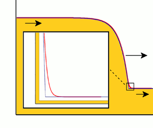
In phase space, the monoclinal wave is represented as a heteroclinic orbit connecting the saddle's stable manifold with the nearest (always repelling) manifold of the unstable node (see figure 3) (Razis et al. Reference Razis, Kanellopoulos and van der Weele2018, Reference Razis, Kanellopoulos and van der Weele2019). This means that the reason for the granular monoclinal wave to exist (from the dynamical systems perspective) is the presence of the stable manifold of the saddle point. The exact position, i.e. the specific negative slope with respect to the horizontal axis, of that manifold as the value of  $\tilde {h}_{+}$ varies determines the entire shape of the granular monoclinal wave.
A granular monoclinal wave profile (a) and its phase space depiction (b). The two uniform plateaus  $\tilde {h}_{-}=1$ and $\tilde {h}=\tilde {h}_{+}$ correspond to the fixed points $(1,0)$ (unstable node) and $(\tilde {h}_{+}, 0)$ (saddle), respectively. The granular monoclinal wave connecting these plateaus is represented in phase space as a heteroclinic orbit connecting the two fixed points. The background grey arrows, which denote the vector field, as well as the added black arrows, show that the orbit is repelled by the (unstable) manifold of the node and attracted by the saddle's stable manifold. The manifolds are denoted by the thin black lines. The system parameters are taken from Russell et al. (Reference Russell, Johnson, Edwards, Viroulet, Rocha and Gray2019): $\zeta _1=21.27^{\circ }, \zeta _2=33.89^{\circ }, \mathcal {L}=0.2351\ \textrm {mm}, \varGamma =0.0, \beta =0.143, \beta _{*}=0.19$ and the arbitrary value of $\zeta =25^{\circ }$ is used.

The contribution of the unstable node at  $(\tilde {h},\tilde {s})=(1,0)$ is rather simple by comparison. Its trace and its determinant are always positive, repelling any initial condition in its neighbourhood. The saddle has a more interesting contribution. In a two-dimensional phase space, the two manifolds of a saddle are rotated as the trace of the Jacobian matrix (evaluated at the saddle point) varies, while the always negative determinant regulates the relative angle between the two manifolds. This general behaviour is depicted in figure 4 for a minimal dynamical system. The saddle point lies at the origin while the manifolds are the straight lines that intersect with it. In figure 4(a,b), the trace of the corresponding Jacobian matrix is kept constant at $\textrm {Tr}=0$ while the determinant becomes smaller, from $\textrm {Det}=-1$ in figure 4(a) to $\textrm {Det}=-2$ in figure 4(b). Evidently, the two manifolds move away from each other with respect the $x$ axis and the angle $\alpha$ increases without any rotation. On the other hand, in figure 4(c,d) where the determinant is kept constant at $\textrm {Det}=-1$ and the trace changes values from $\textrm {Tr}=1$ in figure 4(c) to $\textrm {Tr}=-1$ in figure 4(d), the relative distance of the manifolds is kept intact but they are rotated. More specifically, the angle $\alpha$ increases as the trace becomes smaller.
The relative position of the manifolds of a saddle, in a minimal two-dimensional dynamical system, for various values of the trace and the determinant of the corresponding Jacobian matrix. (a,b) As the trace is kept fixed at  $\textrm {Tr}=0$ and the determinant becomes smaller, from $\textrm {Det}=-1$ in (a) to $\textrm {Det}=-2$ in (b), the manifolds diverge without any rotation. This also leads to the increase of the angle $\alpha$. (c,d) When the (always negative) determinant is kept constant at $\textrm {Det}=-1$ and the trace becomes smaller, from $\textrm {Tr}=1$ in (c) to $\textrm {Tr}=-1$ in (d), the manifolds are rotated around the origin keeping their relative distance intact. Also here the angle $\alpha$ increases.

Back to our system, the analytical expression of the determinant, evaluated at the saddle point  $(\tilde {h}_{+},0)$, as a function of $\tilde {h}_{+}$ is
 \begin{align}
&\textrm{Det}\,J\rvert_{(\tilde{h}_{+},0)}={-}\left.\dfrac{\partial g}{\partial \tilde{h}}\right\vert_{(\tilde{h}_{+},0)} \nonumber\\
&\quad= C(\zeta)\frac{({Fr}_{-}+\varGamma)\tilde{h}_{+}^{3/2}+(-\frac{2}{3}
Fr_{-}-\varGamma)\tilde{h}_{+}^{1/2}+(Fr_{-}+\varGamma)\tilde{h}_{+}^{2} +
(-\frac{2}{3} Fr_{-}-\varGamma)\tilde{h}_{+}-\frac{2}{3}{Fr}_{-}}{\tilde{h}_{+}^{2}
(({Fr}_{-}+\varGamma)\tilde{h}_{+}^{1/2}+({Fr}_{-}+\varGamma)\tilde{h}_{+}+{Fr}_{-})},
\end{align}
\begin{align}
&\textrm{Det}\,J\rvert_{(\tilde{h}_{+},0)}={-}\left.\dfrac{\partial g}{\partial \tilde{h}}\right\vert_{(\tilde{h}_{+},0)} \nonumber\\
&\quad= C(\zeta)\frac{({Fr}_{-}+\varGamma)\tilde{h}_{+}^{3/2}+(-\frac{2}{3}
Fr_{-}-\varGamma)\tilde{h}_{+}^{1/2}+(Fr_{-}+\varGamma)\tilde{h}_{+}^{2} +
(-\frac{2}{3} Fr_{-}-\varGamma)\tilde{h}_{+}-\frac{2}{3}{Fr}_{-}}{\tilde{h}_{+}^{2}
(({Fr}_{-}+\varGamma)\tilde{h}_{+}^{1/2}+({Fr}_{-}+\varGamma)\tilde{h}_{+}+{Fr}_{-})},
\end{align}
where the prefactor  $C(\zeta )$ is given by
 \begin{equation} C(\zeta) =\frac{27\left(\tan(\zeta)-\tan(\zeta_1)\right)\left(\tan(\zeta)-\tan(\zeta_2)\right)}{4 \tan(\zeta)\left(\tan(\zeta_2)-\tan(\zeta_2)\right)}. \end{equation}
Equation (4.1) expresses a negative, monotonically increasing function for  $0<\tilde {h}_{+}<1$ and $\beta _{*}\leqslant {Fr}<{Fr}_{{cr}}$ (see figure 5). This means that as the two plateaus of the granular monoclinal wave come closer to each other ( $\tilde {h}_{+}$ approaches $1$) the determinant of the saddle approaches zero. This implies that the slope of the stable manifold has the tendency to decrease as the fixed points come closer to each other.
Plot of the determinant (4.1) (red curve) and the trace (4.3) (blue curve) of the Jacobian matrix evaluated at the saddle point  $(\tilde {h},\tilde {s})=(\tilde {h}_{+},0)$ as a function of $\tilde {h}_{+}$ for fixed Froude number ${Fr}=0.6$. The system parameters are taken from Russell et al. (Reference Russell, Johnson, Edwards, Viroulet, Rocha and Gray2019): $\zeta _1=21.27^{\circ }, \zeta _2=33.89^{\circ }, \mathcal {L}=0.2351\ \textrm {mm}, \varGamma =0.0, \beta =0.143, \beta _{*}=0.19$ and the arbitrary value of $\zeta =25^{\circ }$ is used.

The trace of the Jacobian matrix evaluated at the saddle point is given by
 \begin{equation} \textrm{Tr}_{(\tilde{h}_{+},0)}J \equiv \left.\frac{\partial g}{\partial \tilde{s}}\right\vert_{(\tilde{h}_{+},0)} = \frac{R\tilde{h}_{+}^{3/2} ( 1 - {Fr}_{-}^{2} (\tilde{c}-1)^{2} \tilde{h}_{+}^{{-}3} )}{{Fr}_{-}^{2} (\tilde{c}-1)}. \end{equation}
 In figure 5 the value of the trace is depicted for fixed Froude number value  ${Fr}=0.6$ and parameter values taken from Russell et al. (Reference Russell, Johnson, Edwards, Viroulet, Rocha and Gray2019). As expected, the trace of the saddle can be positive, negative or even zero as the value of $\tilde {h}_{+}$ varies. The slope of the stable manifold becomes milder as the trace increases its value and vice versa, in full correspondence with the effects of the determinant. In fact, when $\textrm {Tr}_{(\tilde {h}_{+},0)}J = 0$, the two manifolds of the saddle are fully symmetric as far as the slopes of its manifolds are concerned (locally near the saddle point), as the eigenvalues have the same absolute value (but opposite sign).
4.2. Mild and steep granular monoclinal waves
The vanishing of the saddle's trace constitutes a criterion that can be used to classify the granular monoclinal waves, in the sense that it determines the interval of validity of the first-order approximation of the equation of motion (3.5). If we assume the inviscid limit ( $\nu (\zeta )=0$), then the non-dimensional equation (3.5) takes the form
 \begin{equation} \frac{\textrm{d} \tilde{h}}{\textrm{d} \tilde{\xi}}= \frac{\mu(\tilde{h})-\tan \zeta}{{Fr}_{-}^{2} (\tilde{c}-1)^{2} \tilde{h}^{{-}3}-1} \end{equation}
which, with (3.13), can also be written as
 \begin{equation} \frac{\textrm{d} \tilde{h}}{\textrm{d} \tilde{\xi}}= \tilde{s}_{f}= \frac{\left(\tan \zeta-\mu(\tilde{h})\right)R\tilde{h}^{3/2}}{\textrm{Tr}_{(\tilde{h},0)}J\,{Fr}_{-}^{2} (\tilde{c}-1)}. \end{equation}
Equation (4.5) constitutes a dimensionless and more general form (due to the inclusion of the  $\small {\varGamma }$ offset) of (4.1) from Razis et al. (Reference Razis, Kanellopoulos and van der Weele2018), where the authors investigate the region of validity of the inviscid description for the granular monoclinal wave.
Now, the trace of the unstable node is always positive,  $\textrm {Tr}_{(1,0)}J>0$, and thus when also $\textrm {Tr}_{(\tilde {h}_{+},0)}J>0$ holds, it means that the approximate trajectory of the granular monoclinal wave in phase space, given by (4.5), does not encounter any singularity in the interval $\tilde {h}_{+}\leqslant \tilde {h}\leqslant 1$ ( $\tilde {c}$ is always larger than $1$ in the same interval). Indeed, in this case, and especially if $\textrm {Tr}_{(\tilde {h}_{+},0)}J$ is well above zero, one can safely use the first-order approximation rather than (3.5) (see figure 6a). In fact, one can find here, to a very good approximation, the orbit of the granular monoclinal wave in phase space algebraically, from the right-hand side of (4.5), without solving the dynamical system (3.9). On the other hand, if $\textrm {Tr}_{(\tilde {h}_{+},0)}J<0$, (4.5) will produce a singularity inside the interval $\tilde {h}_{+}\leqslant \tilde {h}\leqslant 1$, rendering the inviscid approximation invalid, as can be seen in figure 6(c). The critical state is witnessed in figure 6(b), where we set $\tilde {h}=\tilde {h}_{+}+0.001$ (to achieve visualization for this case we must deviate slightly from $\tilde {h}=\tilde {h}_{+}$ and $\textrm {Tr}_{(\tilde {h}_{+},0)}J=0$). Here, the use of the inviscid approximation is still marginally possible but, as can be seen in the inset, is inadvisable. The above analysis prompts us to classify the monoclinal waves into two major categories, the mild (M) and the steep (S), depending on whether the sign of the trace of the Jacobian matrix evaluated at the saddle $(\tilde {h}_{+}, 0)$ is positive or negative, respectively.
The classification of the granular monoclinal waves for fixed Froude number  $Fr=0.6 < Fr_{{cr}}=2/3$. The threshold value of $\tilde {h}_{+}$, taken from (4.6), is $\tilde {h}_{+,{thres}}=0.6771243445$. (a) Mild regime. For $\tilde {h}_{+}=0.75>\tilde {h}_{+,{thres}}$ we witness that the heteroclinic orbit, representing the monoclinal wave in phase space (red thick curve), is in very good agreement with the inviscid approximation given by (4.5) (dark blue thin curve). The $\tilde {h}$ value for which the first-order approximation becomes singular is well before $\tilde {h}_{+}$ (vertical line), validating its use. The good agreement can be seen also in the corresponding profile depicted in the right-hand panel. There, the area of interest is magnified in the inset in order to visualize the small differences. (b) Critical regime. At $\tilde {h}_{+}=\tilde {h}_{+,{thres}}$ the first-order approximation is marginally valid, as the singular point lies at $\tilde {h} =\tilde {h}_{+}$ (the plots are generated by setting $\tilde {h}_{+}=0.678=\tilde {h}_{+,{thres}}+0.001$ in order to enable the visualization of this case). (c) Steep regime. Here, when $\tilde {h}_{+}=0.6 < \tilde {h}_{+,{thres}}$, the singularity lies inside the interval $\tilde {h}_{+}\leqslant \tilde {h}\leqslant 1$, rendering the first value approximation invalid. The system parameters are taken from Russell et al. (Reference Russell, Johnson, Edwards, Viroulet, Rocha and Gray2019): $\zeta _1=21.27^{\circ }, \zeta _2=33.89^{\circ }, \mathcal {L}=0.2351\ \textrm {mm}, \varGamma =0.0, \beta =0.143, \beta _{*}=0.19$ and the arbitrary value of $\zeta =25^{\circ }$ is used.

The algebraic expression of the threshold height of the lower plateau  $\tilde {h}_{+,{thres}}$ with respect only to incoming Froude number ${Fr}_{-}$ can be found analytically by solving the equation $\textrm {Tr}_{(\tilde {h}_{+},0)}J=0$ given in (4.3) with the help of (3.7). Discarding the two complex solutions and the one real solution that gives $\tilde {h}_{+,{thres}}>1$, we conclude
 \begin{equation} \tilde{h}_{+,{thres}}= \frac{-{Fr}_{-}+\left({-}3({Fr}_{-}+\varGamma-1)({Fr}_{-}-\varGamma/3+1/3)\right)^{1/2}+\varGamma-1}{2( {Fr}_{-}+\varGamma-1)}. \end{equation}
 At the same time, however, one must take into account the lower boundary for the fully dynamic regime,  $\beta _{*}\leqslant {Fr}_{+}$, which dictates the minimum height of the lower plateau $\tilde {h}_{+}$. Equation (2.10) can be written in dimensionless variables as
 \begin{equation} \tilde{h}_{+,{min}}= \frac{\beta_{*}+\varGamma}{{Fr}_{-}+\varGamma}. \end{equation}
A combined plot of (4.6) together with (4.7) is depicted in figure 7 for parameter values taken from Russell et al. (Reference Russell, Johnson, Edwards, Viroulet, Rocha and Gray2019). The dark shaded area below  $\tilde {h}_{+,{min}}$ (blue curve) denotes the values of Froude number and $\tilde {h}_{+}$ for which the regime is not fully dynamic. The light shaded region, which lies above $\tilde {h}_{+,{min}}$ and to the right of $\tilde {h}_{+,{thres}}$ (red curve), is labelled with the letter ‘S’ and represents the area where the steep granular monoclinal waves will be formed. There, the use of the second-order differential equation (3.5) is the only valid choice. On the other hand, the region labelled with the letter ‘M’, above the $\tilde {h}_{+,{min}}$ curve and to the left of the $\tilde {h}_{+,{thres}}$ curve, is the mild regime where the granular monoclinal wave can be approximately described by the inviscid limit (4.4). The gradient grey shading near the $\tilde {h}_{+,{thres}}$ curve reflects the fact that the inviscid approximation (4.4) becomes increasingly inaccurate. The intersection of the two curves is found by setting $\tilde {h}_{+,{thres}}=\tilde {h}_{+,{min}}$. For Froude number values smaller than $Fr\approx 0.5$ here, the granular moniclinal waves are exclusively of the mild type.
Phase diagram showing  $\tilde {h}_{+,{thres}}$ (red curve) together with $\tilde {h}_{+,{min}}$ (blue curve) as a function of the incoming Froude number ( ${Fr}_{-}$). The dark shaded region denotes the area where the flow is not fully dynamic. The letter ‘M’ above the $\tilde {h}_{+,{min}}$ curve and to the left of the $\tilde {h}_{+,{thres}}$ curve denotes the area where the mild granular monoclinal waves appear, while the letter ‘S’ to the right of the $\tilde {h}_{+,{thres}}$ curve and above the $\tilde {h}_{+,{min}}$ curve (light shaded area) denotes the steep regime. The gradient shading inside the mild regime represents the increasing lack of accuracy of the inviscid approximation close to the $\tilde {h}_{+,{thres}}$ curve. The system parameters are taken from Russell et al. (Reference Russell, Johnson, Edwards, Viroulet, Rocha and Gray2019): $\zeta _1=21.27^{\circ }, \zeta _2=33.89^{\circ }, \mathcal {L}=0.2351\ \textrm {mm}, \varGamma =0.0, \beta =0.143, \beta _{*}=0.19$.

The above classification of the granular monoclinal waves into two regimes, the mild and the steep, must be seen mainly from a mathematical point of view. Indeed, the viscous equation of motion, (3.5), is capable of fully describing dynamic granular monoclinal waves (as well as all the other waveforms, given the appropriate parameter values) regardless of to which regime they belong. The element that makes this classification important, combined with the dynamical systems view, is that in the mild regime we can approximate, quite accurately, the granular monoclinal wave in phase space, without solving the full system but by directly plotting (4.5) as a function of  $\tilde {h}$. This constitutes an insightful and direct way to reveal the dynamics of any granular monoclinal wave in the mild regime.
4.3. A case study
It is conceivable that an experimental set-up can be constructed, in which fully dynamic granular monoclinal waves can be detected despite the fact that the chosen material displays a non-zero  $\varGamma$ offset. For that reason, a case study of a hypothetical material that includes a $\varGamma$ offset and is nevertheless capable of establishing this waveform is studied in this subsection. The parameter values of Edwards et al. (Reference Edwards, Viroulet, Kokelaar and Gray2017) are adopted with the exception of the $\varGamma$ offset value. Here we take $\varGamma =0.1$ (instead of $\varGamma =0.4$), and so the full set of the parameter values becomes: $\zeta _1=31.1^{\circ }, \zeta _2=47.5^{\circ }, \mathcal {L}=0.44\ \textrm {mm}, \beta =0.63, \beta _{*}=0.466, \varGamma =0.1$. In addition, the value of $\zeta =33.0^{\circ }$ is used. The critical Froude number in this case, see (3.18), is $Fr_{{cr}}=0.6$, and thus the fully dynamic interval is restricted to $0.466\leqslant Fr<0.6$. Using equation (4.7), the corresponding interval of validity for $\tilde {h}_{+}$ is found to be $0.83235\leqslant \tilde {h}_{+}<1$.
Taking these values into consideration, the incoming Froude number is chosen to be  ${Fr}_{-}=0.58$, while the corresponding lower plateau threshold that separates the mild from the steep regime, see (4.6), is $\tilde {h}_{+,{thres}}=0.876359$. In figure 8 the classification of the granular monoclinal waves for this hypothetical material is depicted. In figure 8(a) where the value $\tilde {h}_{+}=0.9>\tilde {h}_{+,{thres}}$ is chosen, one can see a mild granular monoclinal wave, as expected. In the right-hand panel, the orbit's excellent agreement with the inviscid approximation is witnessed. In figure 8(b) the near-critical case is presented: $\tilde {h}_{+}=0.8765=\tilde {h}_{+,{thres}}+0.0002$. Finally, the steep case can be seen in figure 8(c) where $\tilde {h}_{+}=0.85<\tilde {h}_{+,{thres}}$. Comparing these results with the findings of figure 6, the two systems are qualitatively identical; the differences are only quantitative. This is evident also in figure 9 where the corresponding $\tilde {h}_{+,{thres}}$ curve is plotted along with the corresponding $\tilde {h}_{+,{min}}$ curve, as a function of the incoming Froude number, for this hypothetical set-up.
Granular monoclinal waves in our hypothetical set-up for fixed Froude number  $Fr=0.58 < Fr_{{cr}}=0.6$ and thus, from (4.6), $\tilde {h}_{+,{thres}}=0.876359$. (a) Mild regime. For $\tilde {h}_{+}=0.90>\tilde {h}_{+,{thres}}$ the heteroclinic orbit (red thick curve) is in very good agreement with the inviscid approximation given by (4.5) (dark blue thin curve), as can be especially seen in the inset of the profile plot in the right-hand panel. (b) Critical regime. At $\tilde {h}_{+}=\tilde {h}_{+,{thres}}+0.0002$ the first-order approximation is marginally valid. (c) Steep regime. Here, when $\tilde {h}_{+}=0.85 < \tilde {h}_{+,{thres}}$, the singularity lies inside the interval $\tilde {h}_{+}\leqslant \tilde {h}\leqslant 1$, making the full second-order (viscous) expression necessary. The system parameter values are hypothetical based on measurements of Edwards et al. (Reference Edwards, Viroulet, Kokelaar and Gray2017): $\zeta _1=31.1^{\circ }, \zeta _2=47.5^{\circ }, \zeta =32.7^{\circ }, \mathcal {L}=0.44\ \textrm {mm}, \beta =0.63, \beta _{*}=0.466, \varGamma =0.1$ and the arbitrary value of $\zeta =33^{\circ }$ is used.

Phase diagram showing  $\tilde {h}_{+,{thres}}$ (red curve) together with $\tilde {h}_{+,{min}}$ (blue curve) as a function of the incoming Froude number for the hypothetical set-up of § 4.3. As in figure 7, the dark shaded region denotes the area where the dynamic regime is impossible. The letter ‘M’ above the $\tilde {h}_{+,{min}}$ curve and to the left of the $\tilde {h}_{+,{thres}}$ curve denotes the area where the mild granular monoclinal waves appear, while the light shaded area with the letter ‘S’ to the right of the $\tilde {h}_{+,{thres}}$ curve and above the $\tilde {h}_{+,{min}}$ curve denotes the steep regime. The gradient shading inside the mild regime represents the increasing lack of accuracy of the inviscid approximation close to the $\tilde {h}_{+,{thres}}$ curve. The system parameter values are: $\zeta _1=31.1^{\circ }, \zeta _2=47.5^{\circ }, \mathcal {L}=0.44\ \textrm {mm}, \beta =0.63, \beta _{*}=0.466, \varGamma =0.1$.

The phase diagrams of figures 7 and 9 provide a guideline for further study of granular monoclinal waves. Equations (4.6) and (4.7) have a simple algebraic form and they depend only on the parameters  $\varGamma$ and $\beta _{*}$. This fact makes them a very useful tool for theorists and experimentalists alike.
5. Concluding remarks
In this paper, the mathematical properties of the granular monoclinal wave are clarified. As a travelling waveform, it can be well described by casting the granular Saint-Venant equations into a two-dimensional dynamical system. In order to make the formulation as general as possible, the modified expression of the friction coefficient introduced by Edwards et al. (Reference Edwards, Viroulet, Kokelaar and Gray2017), which includes the  $\varGamma$ offset, has been adopted.
Exploiting the stability analysis findings, the critical Froude number above which the uniform flow becomes unstable was determined as a function of the  $\varGamma$ offset (equation (3.18)). From that relation it is clear that – given the fact that the granular monoclinal wave is a travelling shock structure that connects two plateaus of steady and uniform flow – a material with $\textstyle \varGamma =0$ is more likely to develop such waves.
Based on our understanding of the properties of the saddle's stable manifold, a classification of the granular monoclinal waves was possible. It was shown that when the trace of the saddle is positive, the actual profile can be approximated by the inviscid limit (4.4) of the full, viscous equation of motion (3.5) (mild regime). On the other side of the spectrum, when the saddle's trace is negative, this approximation becomes invalid (steep regime). In the same context, an analytical expression relating the height of the lower plateau with the value of the incoming Froude number that separates these two regimes is given (4.6). Along with the curve that determines the minimum level of  $\tilde {h}_{+}$ in the fully dynamic regime (4.7), they constitute a map of the dynamical properties of the granular monoclinal waves.
A study of the possible formation of granular monoclinal waves in a hypothetical material with non-zero  $\varGamma$ offset is included in this paper. The results were qualitatively very similar to those obtained with the experimental set-up of Russell et al. (Reference Russell, Johnson, Edwards, Viroulet, Rocha and Gray2019), which lacks the $\varGamma$ offset parameter, illustrating the relevance of the case study in question.
In order to address the important issue of the stability of the solutions obtained from the dynamical system, one must return to the original time-dependent PDEs, i.e. the granular Saint-Venant equations (2.1)–(2.2). The stability of the monoclinal profiles found earlier can be demonstrated by inserting them, in perturbed form, as initial conditions into these PDEs. In figure 10, as an example, we show the time evolution of the thus perturbed ‘mild’ monoclinal wave. The perturbation (a small surplus of material in the shape of a Gaussian-like bump) is seen to disappear in the course of time, yielding again the unperturbed profile which remains unchanged afterwards.
Stability of a granular monoclinal wave which constitutes a solution of (3.3) with  $Fr=0.6$ and a height $h_{+}$ corresponding to $\tilde {h}_{+}=0.92$ (mild regime): an initial perturbation (black thin curve) is positioned on the wave's upper plateau and its evolution is computed from the granular Saint-Venant equations (2.1)–(2.2). The perturbation is seen to diminish in time, and after $180$ s we witness that the monoclinal wave has recovered its initial shape. The red dashed curve denotes the unperturbed initial monoclinal wave, and is presented here for direct comparison with the solution taken from the PDEs (solid lines). The evolution of the system has been evaluated using the method of lines (Schiesser Reference Schiesser1991; Razis et al. Reference Razis, Kanellopoulos and van der Weele2018), with a computational space step of $\Delta x = 0.01$ m over a total length of $x_{{max}} = 50$ m. The system parameters are taken from Russell et al. (Reference Russell, Johnson, Edwards, Viroulet, Rocha and Gray2019): $\zeta _1=21.27^{\circ }, \zeta _2=33.89^{\circ }, \mathcal {L}=0.2351\ \textrm {mm}, \varGamma =0.0, \beta =0.143, \beta _{*}=0.19$ and the arbitrary value of $\zeta =25^{\circ }$ is used.

As a final remark, it may be noted that this analysis applies to normal fluids too. The modified Saint-Venant equations introduced by Kranenburg (Reference Kranenburg1992) in the context of the evolution of roll waves in normal fluids (see also Yu & Kevorkian Reference Yu and Kevorkian1992; Yu, Kevorkian & Haberman Reference Yu, Kevorkian and Haberman2000; Balmforth & Mandre Reference Balmforth and Mandre2004) give rise to a similar dynamical system with many analogies. This will be reported in a forthcoming publication.
Acknowledgements
I cordially thank Professor K. van der Weele (University of Patras, Greece) and Dr D. Razis for their interest in this work and for their very insightful advice.
Funding
This research is co-financed by Greece and the European Union (European Social Fund – ESF) through the Operational Programme ‘Human Resources Development, Education and Lifelong Learning’ in the context of the project ‘Reinforcement of Postdoctoral Researchers – 2nd Cycle’ (MIS-5033021), implemented by the State Scholarships Foundation (IKY).
Declaration of interests
The author reports no conflict of interest.


 Open access