


1. Introduction
The usual boundary condition at a solid–fluid boundary is the no-slip condition,  $\boldsymbol {u}_t - \boldsymbol {v}_t = \boldsymbol {0}$, where $\boldsymbol {u}_t$ and $\boldsymbol {v}_t$ are the tangential velocities of the fluid and solid, respectively. The no-slip condition assumes that there is no jump in tangential velocity, or slip, across the boundary. However, most real fluid–solid boundaries will exhibit some small amount of slip (Thompson & Troian Reference Thompson and Troian1997), which is described using the partial-slip boundary condition,
 \begin{equation} \boldsymbol{u}_t - \boldsymbol{v}_t = \lambda \frac{\partial \boldsymbol{u}_t}{\partial n},\end{equation}
where  $\lambda$ is the slip length, and $n$ is the direction normal to the wall. While the slip length is often negligible, there are a range of practical flow configurations where the slip length must be considered, such as in microfluidic applications (Lauga, Brenner & Stone Reference Lauga, Brenner and Stone2007), dilute-gas flows (Morris, Hannon & Garcia Reference Morris, Hannon and Garcia1992) or the motion of a contact line (Thompson & Robbins Reference Thompson and Robbins1989).
The partial-slip boundary condition is also used to model superhydrophobic surfaces, which have an apparent slip length (Cottin-Bizonne et al. Reference Cottin-Bizonne, Barrat, Bocquet and Charlaix2003; Tretheway & Meinhart Reference Tretheway and Meinhart2004; Gao & Feng Reference Gao and Feng2009). Such surfaces have been found to reduce skin-friction drag in both laminar (Lee, Choi & Kim Reference Lee, Choi and Kim2016) and turbulent (Gose et al. Reference Gose, Golovin, Boban, Mabry, Tuteja, Perlin and Ceccio2018; Park, Choi & Kim Reference Park, Choi and Kim2021) flows and can reduce flow separation, thereby reducing form drag (Jetly, Vakarelski & Thoroddsen Reference Jetly, Vakarelski and Thoroddsen2018; Mollicone et al. Reference Mollicone, Battista, Gualtieri and Casciola2022) and preventing stall (Sooraj, Jain & Agrawal Reference Sooraj, Jain and Agrawal2019).
The partial-slip boundary condition also generalises the free-slip boundary condition, which occurs at a free surface. Contaminated surfaces display behaviour intermediate between the no-slip and free-slip boundary conditions (Tryggvason et al. Reference Tryggvason, Abdollahi-Alibeik, Willmarth and Hirsa1992; Hirsa & Willmarth Reference Hirsa and Willmarth1994; Tsai & Yue Reference Tsai and Yue1995), depending on the variation of the surfactant concentration, and may therefore be approximated using the partial-slip boundary condition.
Vorticity dynamics provides a useful alternative viewpoint for understanding the dynamics of various flows, and often provides greater insight than momentum considerations alone (Lighthill Reference Lighthill1963). Zhu et al. (Reference Zhu, Zhu, Su, Zou, Liu, Shi and Wu2014) have discussed the partial-slip boundary condition from the perspective of vorticity dynamics, providing expressions for the surface vorticity and the boundary vorticity flux. They illustrate the usefulness of vorticity dynamics in understanding boundary layer control. Specifically, flow separation is attributed to a surplus of vorticity in the boundary layer. Partial-slip boundaries reduce the boundary vorticity flux, therefore reducing flow separation.
The present authors have recently developed a general formulation of boundary vorticity dynamics (Terrington, Hourigan & Thompson Reference Terrington, Hourigan and Thompson2022b), which does not explicitly depend on the tangential boundary conditions, and can therefore be applied to a wide range of interfaces and boundaries, including no-slip walls, free surfaces and fluid–fluid interfaces. The present paper examines the dynamics of vorticity at partial-slip boundaries under this formulation.
Our formulation treats the slip velocity at a partial-slip boundary as representing a vortex sheet, or more precisely as a surface density of vector circulation (Terrington et al. Reference Terrington, Hourigan and Thompson2022b). There are two main benefits to this approach. First, the total vector circulation – including both the total vorticity of the fluid and the vector circulation of the interface vortex sheet – is generally conserved. While local creation of vector circulation may occur within the interface vortex sheet, this will be balanced by an equal creation of opposite-signed vector circulation elsewhere.
Second, we provide a general mechanism for the generation of vector circulation within the interface vortex sheet, which applies equally to free-slip, no-slip and partial-slip boundaries. Vector circulation is generated by the inviscid relative acceleration between the fluid and the boundary, caused by either a tangential pressure gradient or acceleration of the solid wall. The rate of generation of vector circulation does not depend on either the fluid viscosity or the degree of slip at the wall.
While neither viscosity nor slip length affect the creation of vector circulation, they do govern how vector circulation is redistributed between the interface vortex sheet and the total vorticity of the fluid. The partial-slip boundary condition provides a relationship between the density of vector circulation in the interface vortex sheet and the tangential boundary vorticity. The viscous boundary vorticity flux transfers vector circulation between the interface vortex sheet and the fluid interior to maintain this condition. In the limiting case of a no-slip boundary, all vector circulation is diffused into the fluid as vorticity, since the no-slip boundary cannot sustain an interface vortex sheet.
The structure of this paper is as follows. First, in § 2 we discuss the theory of vorticity and vector circulation dynamics at partial-slip boundaries. Then, in § 3 we examine the interaction between a vortex ring and a partial-slip wall, to illustrate the behaviour of vorticity at partial-slip boundaries. Finally, concluding remarks are made in § 4.
2. Theory
In this section we discuss the dynamics of vorticity and vector circulation at partial-slip boundaries. The structure is as follows. First, we discuss the equations of motion and boundary conditions from the perspective of linear momentum in § 2.1. Then, we introduce the vorticity and the interface vortex sheet at a partial-slip boundary in § 2.2. We then discuss the dynamics of vorticity and the interface vortex sheet in § 2.3. Finally, the boundary conditions for vorticity at a partial-slip boundary are discussed in §§ 2.4 and 2.5.
2.1. Dynamics of linear momentum
We assume incompressible flow of a constant-viscosity Newtonian fluid, which is governed by the continuity and Navier–Stokes equations:
 $$\begin{gather} \boldsymbol{\nabla} \boldsymbol{\cdot} \boldsymbol{u} = 0, \end{gather}$$
 $$\begin{gather}\frac{\mathrm d \boldsymbol{u}}{\mathrm d t} ={-}\boldsymbol{\nabla} p + \frac{1}{Re} \boldsymbol{\nabla}^2 \boldsymbol{u}. \end{gather}$$
Quantities have been non-dimensionalised by a length scale  $L$, velocity scale $U$ and the fluid density $\rho$. The fluid viscosity is denoted $\mu$ and $Re = \rho U L/\mu$ is the Reynolds number. The dimensionless pressure $p$ includes both the dimensional pressure $p^*$ and the body force potential $\phi _g^*$, as $p = (p^* + \phi _g^*)/\rho U^2$.
The general form of the partial-slip boundary condition is (Bazant & Vinogradova Reference Bazant and Vinogradova2008)
 \begin{equation} \boldsymbol{u} - \boldsymbol{v} = {{\boldsymbol{\mathsf{M}}}} \boldsymbol{\cdot} (\boldsymbol{\hat{s}} \boldsymbol{\cdot} {{\boldsymbol{\mathsf{T}}}}),\end{equation}
where  ${{\boldsymbol{\mathsf{T}}}}$ is the viscous stress tensor, ${{\boldsymbol{\mathsf{M}}}}$ is the interfacial mobility tensor and $\boldsymbol {\hat {s}}$ is the unit normal to the boundary directed into the fluid. This form of the partial-slip boundary condition relates both the slip velocity and the permeability of the wall to the applied surface stress.
The tensor  ${{\boldsymbol{\mathsf{M}}}}$ is useful for surfaces where the degree of slip depends on the direction, such as patterned microsurfaces. In the present work, we assume no permeability of the surface, i.e.
 \begin{equation} \boldsymbol{\hat{s}} \boldsymbol{\cdot} (\boldsymbol{u} - \boldsymbol{v}) = 0, \end{equation}
and that the surface slip is isotropic. For isotropic slip, and for a Newtonian fluid, we can replace the tensor  ${{\boldsymbol{\mathsf{M}}}}$ with a scalar slip length $\lambda$ (Legendre, Lauga & Magnaudet Reference Legendre, Lauga and Magnaudet2009; Zhu et al. Reference Zhu, Zhu, Su, Zou, Liu, Shi and Wu2014)
 \begin{equation} \boldsymbol{\hat{s}} \times (\boldsymbol{u} - \boldsymbol{v}) = Kn \boldsymbol{\hat{s}} \times (\boldsymbol{\hat{s}} \boldsymbol{\cdot} \boldsymbol{\nabla} \boldsymbol{u} + \boldsymbol{\nabla} \boldsymbol{u} \boldsymbol{\cdot} \boldsymbol{\hat{s}}), \end{equation}
where  $Kn = \lambda /L$ is the Knudsen number (Legendre et al. Reference Legendre, Lauga and Magnaudet2009). For a non-rotating plane wall, (2.5) reduces to the well-known form given by (1.1).
We can also express the partial-slip boundary condition in terms of a ‘slip coefficient’,  $\alpha = Kn/(1+Kn)$:
 \begin{equation} (1-\alpha) \boldsymbol{\hat{s}} \times (\boldsymbol{u} - \boldsymbol{v}) = \alpha \boldsymbol{\hat{s}} \times (\boldsymbol{\hat{s}} \boldsymbol{\cdot} \boldsymbol{\nabla} \boldsymbol{u} + \boldsymbol{\nabla} \boldsymbol{u} \boldsymbol{\cdot} \boldsymbol{\hat{s}}).\end{equation}
Here  $\alpha = 0$ corresponds to the no-slip boundary condition ( $Kn = 0$) and $\alpha = 1$ corresponds to the free-slip boundary condition ( $Kn = \infty$).
2.2. Vorticity and vector circulation
Vorticity is the curl of velocity,
 \begin{equation} \boldsymbol{ \omega} = \boldsymbol{\nabla} \times \boldsymbol{u}, \end{equation}
and can be interpreted as representing twice the mean rotation rate of an infinitesimal fluid element (Truesdell Reference Truesdell1954). It is often useful to consider the volume integral of vorticity, which is known as the total vorticity (Poincaré Reference Poincaré1893; Truesdell Reference Truesdell1948). Using the generalised Stokes theorem (Truesdell Reference Truesdell1954, (7.3)), the total vorticity contained in a volume  $V$ can be expressed as a surface integral of tangential velocity on the control-volume boundary ( $\partial V$):
 \begin{equation} \boldsymbol{ \varGamma} = \int_V \boldsymbol{ \omega}\, \mathrm d V = \oint_{\partial V} \boldsymbol{\hat{n}} \times \boldsymbol{u} \,\mathrm d S.\end{equation}
Here  $\boldsymbol {\hat {n}}$ is the unit normal vector to $\partial V$, directed out of $V$.
$V$.
Noting that (2.8) is analogous to the relationship between total vorticity and circulation in two dimensions, we refer to the integral on the right-hand side of (2.8) as the vector circulation (Terrington, Hourigan & Thompson Reference Terrington, Hourigan and Thompson2021; Terrington et al. Reference Terrington, Hourigan and Thompson2022b). This is a different quantity to circulation, which is the line integral of velocity along a closed curve, even in three dimensions. Our motivation for introducing the term ‘vector circulation’ to refer to the right-hand side of (2.8), rather than referring to this quantity only as the ‘total vorticity’, is to allow the slip velocity at an interface to be unambiguously interpreted as a kind of vortex sheet.
Specifically, while Wu & Wu (Reference Wu and Wu1993) do not consider a slip velocity to represent a sheet of vorticity, the slip velocity does unambiguously represent a surface density of vector circulation or a boundary vortex sheet (Terrington et al. Reference Terrington, Hourigan and Thompson2021, Reference Terrington, Hourigan and Thompson2022b)
 \begin{equation} \boldsymbol{ \gamma} = \boldsymbol{\hat{s}} \times (\boldsymbol{u} - \boldsymbol{v}), \end{equation}
where  $\boldsymbol { \gamma }$ is the surface density of vector circulation due to the slip velocity at the boundary.
To demonstrate this, we consider the control volume  $V$ illustrated in figure 1. Part of the boundary surface ( $\partial V$) lies on the partial-slip wall $(\partial V)_s$, while the rest of the boundary lies in the fluid interior $(\partial V)_f$. We let $\boldsymbol {u}$ be the fluid velocity, $\boldsymbol {v}$ be the solid velocity and $\boldsymbol {w}$ be the velocity of the control-volume boundary. Since $(\partial V)_s$ must remain on the partial-slip wall, we have the following condition on $(\partial V)_s$:
 \begin{equation} \boldsymbol{u} \boldsymbol{\cdot} \boldsymbol{\hat{s}} = \boldsymbol{v} \boldsymbol{\cdot} \boldsymbol{\hat{s}} = \boldsymbol{w} \boldsymbol{\cdot} \boldsymbol{\hat{s}}. \end{equation}
Control volume  $V$ considered in this work. The boundary is separated into two portions: $(\partial V)_s$, the portion that lies on the partial-slip wall; and $(\partial V)_f$, the portion that lies in the fluid interior. The boundary curve to $(\partial V)_s$ is denoted $\partial I$. Finally, $\boldsymbol {\hat {n}}$ and $\boldsymbol {\hat {s}}$ are the unit normal vectors to $(\partial V)_f$ and $(\partial V)_s$, respectively.

The velocity at  $(\partial V)_s$ is not well defined, and may equal either the fluid velocity $\boldsymbol {u}$ or the solid velocity $\boldsymbol {v}$. To account for this, we let the surfaces $(\partial V)_{s,\boldsymbol {u}}$ and $(\partial V)_{s,\boldsymbol {v}}$ approach $(\partial V)_s$ from the fluid and solid sides, respectively. Taking the limits $(\partial V)_{s,\boldsymbol {u}} \rightarrow (\partial V)_s$ and $(\partial V)_{s,\boldsymbol {v}} \rightarrow (\partial V)_s$ there is a vector circulation contained in the region bounded by these surfaces:
 \begin{equation} \boldsymbol{ \varGamma}_\gamma = \int_{(\partial V)_{s,\boldsymbol{u}}} \boldsymbol{\hat{s}} \times \boldsymbol{u}\, \mathrm d S - \int_{(\partial V)_{s,\boldsymbol{v}}} \boldsymbol{\hat{s}} \times \boldsymbol{v}\,\mathrm d S = \int_{(\partial V)_s} \boldsymbol{ \gamma}\, \mathrm d S. \end{equation}
Also considering the total vorticity of the fluid,
 \begin{equation} \boldsymbol{ \varGamma}_\omega = \int_V \boldsymbol{ \omega}\, \mathrm d V = \int_{(\partial V)_f}\boldsymbol{\hat{n}} \times \boldsymbol{u}\, \mathrm d S - \int_{(\partial V)_{s,\boldsymbol{u}}} \boldsymbol{\hat{s}} \times \boldsymbol{u}\, \mathrm d S, \end{equation}
the total vector circulation includes both the total vorticity of the fluid and the vector circulation in the interface vortex sheet:
 \begin{equation} \boldsymbol{ \varGamma} = \int_{(\partial V)_f}\boldsymbol{\hat{n}} \times \boldsymbol{u}\, \mathrm d S - \int_{(\partial V)_{s,\boldsymbol{v}}} \boldsymbol{\hat{s}} \times \boldsymbol{v}\, \mathrm d S = \boldsymbol{ \varGamma}_\omega + \boldsymbol{ \varGamma}_\gamma.\end{equation}
 We note that discontinuities of tangential velocity have long been identified as vortex sheets (e.g. Lamb Reference Lamb1924; Batchelor Reference Batchelor1967). However, this identification is usually performed by considering a thin surface containing a finite total vorticity, and then allowing the sheet thickness to approach  $\delta \rightarrow 0$, while keeping the total vorticity constant (e.g. Batchelor Reference Batchelor1967, § 2.6). Wu & Wu (Reference Wu and Wu1993) have pointed out that such a vortex sheet is physically different from a slip velocity at a fluid–solid boundary. In particular, the vortex sheet obtained under the limit $\delta \rightarrow 0$ of a thin shear layer implies that fluid elements rotate with an angular velocity $\omega = \infty$, while a slip velocity implies that fluid elements on the boundary slide relative to one another, without rotation.
While a slip velocity does not represent the physical rotation of fluid elements, it does represent a surface density of vector circulation, as defined by the integral on the right-hand side of (2.8). Moreover, interpreting this slip velocity as a kind of boundary vortex sheet generalises a number of useful kinematic properties of the vorticity field, including a generalised divergence-free condition, a generalised Biot–Savart law and a generalised Stokes theorem (Terrington et al. Reference Terrington, Hourigan and Thompson2021, Reference Terrington, Hourigan and Thompson2022b). Recognising these compelling mathematical reasons to interpret the slip velocity as a boundary vortex sheet, the present paper considers the vector circulation – which unambiguously includes both the total vorticity of the fluid and the boundary vortex sheet – to be the primary quantity of interest.
2.3. Dynamics of vector circulation
We have previously developed a general formulation of the creation of vector circulation at generalised fluid–fluid interfaces (Terrington et al. Reference Terrington, Hourigan and Thompson2022b). The present subsection outlines the main results of this formulation. The equations presented in this section are slightly different from those in Terrington et al. (Reference Terrington, Hourigan and Thompson2022b). Specifically, the present paper considers only the total vorticity of the fluid and the vector circulation of the boundary vortex sheet, while the total vorticity of the solid was also considered in Terrington et al. (Reference Terrington, Hourigan and Thompson2022b).
The vorticity transport equation is obtained by taking the curl of (2.2) (Lamb Reference Lamb1924; Batchelor Reference Batchelor1967),
 \begin{equation} \frac{\partial \boldsymbol{ \omega}}{\partial t} + \boldsymbol{u} \boldsymbol{\cdot} \boldsymbol{\nabla} \boldsymbol{ \omega} =\boldsymbol{ \omega} \boldsymbol{\cdot} \boldsymbol{\nabla} \boldsymbol{u} + \nu \boldsymbol{\nabla}^2 \boldsymbol{ \omega}. \end{equation}
The vorticity transport equation can also be expressed in integral form to give the rate of change of total vorticity in the fluid (Truesdell Reference Truesdell1948; Terrington et al. Reference Terrington, Hourigan and Thompson2022b),
 \begin{align} \frac{\mathrm d \boldsymbol{ \varGamma}_\omega}{\mathrm d t} &= \int_{(\partial V)_f} \boldsymbol{ \omega} (\boldsymbol{w} - \boldsymbol{u}) \boldsymbol{\cdot} \boldsymbol{\hat{n}}\, \mathrm d S + \int_{(\partial V)_f} (\boldsymbol{ \omega} \boldsymbol{\cdot} \boldsymbol{\hat{n}})\boldsymbol{u}\, \mathrm d S - \int_{(\partial V)_f}\frac{1}{Re} \boldsymbol{\hat{n}} \times (\boldsymbol{\nabla} \times \boldsymbol{ \omega})\, \mathrm d S \nonumber\\ &\quad - \int_{(\partial V)_s} (\boldsymbol{ \omega} \boldsymbol{\cdot} \boldsymbol{\hat{s}})\boldsymbol{u}\, \mathrm d S + \int_{(\partial V)_s}\frac{1}{Re} \boldsymbol{\hat{s}} \times (\boldsymbol{\nabla} \times \boldsymbol{ \omega})\, \mathrm d S. \end{align}
Using (2.36) from Terrington et al. (Reference Terrington, Hourigan and Thompson2022b), the rate of change of  $\boldsymbol { \varGamma }_\gamma$ is
 \begin{align} \frac{\mathrm d \boldsymbol{ \varGamma}_\gamma}{\mathrm d t} &= \int_{(\partial V)_s}\boldsymbol{ \varSigma}\, \mathrm d S - \int_{(\partial V)_s} \frac{1}{Re} \boldsymbol{\hat{s}} \times (\boldsymbol{\nabla} \times \boldsymbol{ \omega})\, \mathrm d S + \int_{(\partial V)_s}[ (\boldsymbol{ \omega} \boldsymbol{\cdot} \boldsymbol{\hat{s}}) \boldsymbol{u} - (\boldsymbol{ \omega}_v \boldsymbol{\cdot} \boldsymbol{\hat{s}}) \boldsymbol{v} ]\, \mathrm d S \nonumber\\ &\quad -\oint_{\partial I} \left[\frac{1}{2}(\boldsymbol{u} \boldsymbol{\cdot} \boldsymbol{u} - \boldsymbol{v} \boldsymbol{\cdot} \boldsymbol{v}) + (\boldsymbol{ \gamma} \times \boldsymbol{\hat{s}}) \times (\boldsymbol{w} \times \boldsymbol{\hat{t}}) \right]\mathrm d s, \end{align}
where  $\boldsymbol { \varSigma }$ is a surface-density source of vector circulation:
 \begin{equation} \boldsymbol{ \varSigma} ={-} \boldsymbol{\hat{n}} \times \left[\boldsymbol{\nabla} p + \frac{\mathrm d \boldsymbol{v}}{\mathrm d t} \right].\end{equation}
Here  $\boldsymbol { \omega }_v = \boldsymbol {\nabla } \times \boldsymbol {v}$ is the vorticity of the solid body and $\boldsymbol {\hat {t}}$ is the unit tangent vector to $\partial I$. Finally, combining (2.15) and (2.16) gives the balance of total vector circulation, including both the total vorticity of the fluid and the vector circulation contained in the boundary vortex sheet:
 \begin{align} \frac{\mathrm d
\boldsymbol{ \varGamma}}{\mathrm d t} &= \int_{(\partial
V)_s} \boldsymbol{ \varSigma}\, \mathrm d S +
\int_{(\partial V)_f} \boldsymbol{ \omega} (\boldsymbol{w}
- \boldsymbol{u}) \boldsymbol{\cdot} \boldsymbol{\hat{n}}\,
\mathrm d S\nonumber\\
&\quad + \int_{(\partial V)_f} (\boldsymbol{ \omega}
\boldsymbol{\cdot} \boldsymbol{\hat{n}})\boldsymbol{u}\,
\mathrm d S - \int_{(\partial V)_f}\frac{1}{Re}
\boldsymbol{\hat{n}} \times (\boldsymbol{\nabla} \times
\boldsymbol{ \omega})\, \mathrm d S \nonumber\\
&\quad -\int_{(\partial V)_s} (\boldsymbol{ \omega}_v
\boldsymbol{\cdot} \boldsymbol{\hat{s}}) \boldsymbol{v}\,
\mathrm d S - \oint_{\partial I}
\left[\frac{1}{2}(\boldsymbol{u} \boldsymbol{\cdot}
\boldsymbol{u} - \boldsymbol{v} \boldsymbol{\cdot}
\boldsymbol{v}) + (\boldsymbol{ \gamma} \times
\boldsymbol{\hat{s}}) \times (\boldsymbol{w} \times
\boldsymbol{\hat{t}}) \right]\mathrm d s.
\end{align}
\begin{align} \frac{\mathrm d
\boldsymbol{ \varGamma}}{\mathrm d t} &= \int_{(\partial
V)_s} \boldsymbol{ \varSigma}\, \mathrm d S +
\int_{(\partial V)_f} \boldsymbol{ \omega} (\boldsymbol{w}
- \boldsymbol{u}) \boldsymbol{\cdot} \boldsymbol{\hat{n}}\,
\mathrm d S\nonumber\\
&\quad + \int_{(\partial V)_f} (\boldsymbol{ \omega}
\boldsymbol{\cdot} \boldsymbol{\hat{n}})\boldsymbol{u}\,
\mathrm d S - \int_{(\partial V)_f}\frac{1}{Re}
\boldsymbol{\hat{n}} \times (\boldsymbol{\nabla} \times
\boldsymbol{ \omega})\, \mathrm d S \nonumber\\
&\quad -\int_{(\partial V)_s} (\boldsymbol{ \omega}_v
\boldsymbol{\cdot} \boldsymbol{\hat{s}}) \boldsymbol{v}\,
\mathrm d S - \oint_{\partial I}
\left[\frac{1}{2}(\boldsymbol{u} \boldsymbol{\cdot}
\boldsymbol{u} - \boldsymbol{v} \boldsymbol{\cdot}
\boldsymbol{v}) + (\boldsymbol{ \gamma} \times
\boldsymbol{\hat{s}}) \times (\boldsymbol{w} \times
\boldsymbol{\hat{t}}) \right]\mathrm d s.
\end{align} The physical interpretation of various terms in (2.15)–(2.18) was discussed in Terrington et al. (Reference Terrington, Hourigan and Thompson2022b), and will be briefly restated here. The term  $\boldsymbol { \varSigma }$ represents a surface-density source of vector circulation in the interface vortex sheet. Specifically, vector circulation is generated by an inviscid relative acceleration between the fluid and the solid, due to either a tangential pressure gradient or an external acceleration of the solid body. This extends Morton's (Reference Morton1984) inviscid theory of vorticity creation to three-dimensional flows, assuming the slip velocity at the boundary is interpreted as a boundary vortex sheet.
The term  $\int _{(\partial V)_s} ({1}/{Re}) \boldsymbol {\hat {s}} \times (\boldsymbol {\nabla } \times \boldsymbol { \omega })\, \mathrm d S$ in (2.15) and (2.16) is the viscous boundary vorticity flux, which represents the viscous transfer of vector circulation between the interface vortex sheet and the total vorticity of the fluid. Importantly, this term is absent from (2.18), and therefore, viscosity is not involved in the generation of vector circulation.
Note that we have used Lyman's definition of the viscous boundary vorticity flux,  $\boldsymbol { \sigma } =({1}/{Re})\boldsymbol {\hat {s}} \times (\boldsymbol {\nabla } \times \boldsymbol { \omega })$ (Lyman Reference Lyman1990), rather than the alternative Lighthill–Panton definition, $\boldsymbol { \sigma } = -({1}/{Re}) \boldsymbol {\hat {s}} \boldsymbol {\cdot } \boldsymbol {\nabla } \boldsymbol { \omega }$ (Lighthill Reference Lighthill1963; Panton Reference Panton1984). Both definitions predict the same kinematic evolution of the vorticity field, and there is not a clear physical justification to prefer either definition (Terrington et al. Reference Terrington, Hourigan and Thompson2021). For our purposes, we find Lyman's definition preferable, as it allows a completely inviscid description of the creation of vector circulation.
Terms involving  $(\boldsymbol { \omega } \boldsymbol {\cdot } \boldsymbol {\hat {s}})\boldsymbol {u}$ and $(\boldsymbol { \omega }_v \boldsymbol {\cdot } \boldsymbol {\hat {s}})\boldsymbol {v}$ are related to vortex stretching and tilting. Specifically, the terms involving $( \boldsymbol { \omega } \boldsymbol {\cdot } \boldsymbol {\hat {n}}) \boldsymbol {u}$ in (2.15) represent the rate of change of vector circulation in the fluid due to the vortex stretching/tilting term:
 \begin{equation} \int_{(\partial V)_s} -(\boldsymbol{ \omega} \boldsymbol{\cdot} \boldsymbol{\hat{s}})\boldsymbol{u}\mathrm d S + \int_{(\partial V)_f} (\boldsymbol{ \omega} \boldsymbol{\cdot} \boldsymbol{\hat{n}})\boldsymbol{u}\mathrm d S = \int_{V} \boldsymbol{ \omega} \boldsymbol{\cdot} \boldsymbol{\nabla} \boldsymbol{u}\, \mathrm d V. \end{equation}
Therefore, the corresponding term  $\oint _{(\partial V)_s} \boldsymbol {\hat {s}} \boldsymbol {\cdot } [\boldsymbol { \omega } \boldsymbol {u} - \boldsymbol { \omega }_v \boldsymbol {v} ]\, \mathrm d S$ in (2.16) is interpreted as a kind of vortex stretching/tilting occurring in the interface vortex sheet. The total vorticity creation due to vortex stretching and tilting is given by the following terms in (2.18):
 \begin{align} \int_{(\partial V)_f} (\boldsymbol{ \omega} \boldsymbol{\cdot} \boldsymbol{\hat{n}})\boldsymbol{u}\, \mathrm d S -\int_{(\partial V)_s} (\boldsymbol{ \omega}_v \boldsymbol{\cdot} \boldsymbol{\hat{s}}) \boldsymbol{v}\, \mathrm d S = \int_{V} \boldsymbol{ \omega} \boldsymbol{\cdot} \boldsymbol{\nabla} \boldsymbol{u}\, \mathrm d V + \int_{(\partial V)_s} \boldsymbol{\hat{s}} \boldsymbol{\cdot} [\boldsymbol{ \omega} \boldsymbol{u} - \boldsymbol{ \omega}_v \boldsymbol{v} ]\,\mathrm d S. \end{align}
These terms demonstrate that vortex stretching can only produce a net creation of vector circulation if vortex lines intersect the control-volume boundary (Terrington et al. Reference Terrington, Hourigan and Thompson2022b).
The remaining terms in (2.15)–(2.18) describe the transport of vector circulation across the control-volume boundary. Integrals over  $(\partial V)_f$ describe the transport of vorticity in the fluid interior, by either advection ( $\boldsymbol { \omega } (\boldsymbol {w} - \boldsymbol {u}) \boldsymbol {\cdot } \boldsymbol {\hat {n}}$) or viscous diffusion ( $({1}/{Re}) \boldsymbol {\hat {n}} \times (\boldsymbol {\nabla } \times \boldsymbol { \omega })$). Finally, the integral over ( $\partial I$) describes the transport of vector circulation within the interface vortex sheet, along the interface.
Terms in (2.18) are defined only on the control-volume boundary  $\partial V$, and therefore, express a conservation principle for vector circulation (Terrington et al. Reference Terrington, Hourigan and Thompson2022b). The total vector circulation within $V$ can only change if new vector circulation is added at the boundaries – either by the transport of vorticity in the fluid interior $(\partial V)_f$, along the interface vortex sheet $(\partial I)$, by the vortex stretching/tilting terms, or by the creation of vorticity at the boundary ( $\boldsymbol { \varSigma }$). Importantly, if the solid wall is stationary and there is no net external pressure gradient, then there is no net creation of vector circulation. Local creation of vector circulation may occur but this is balanced by the creation of opposite-signed vector circulation elsewhere. This extends a previous result of Poincaré (Reference Poincaré1893) and Truesdell (Reference Truesdell1948), who show that the total vorticity in either an unbound fluid domain or a fluid domain partially bounded by a stationary no-slip wall is constant in time, assuming the vorticity flux terms decay sufficiently at infinity.
2.4. Boundary conditions for surface-tangential vorticity
The general formulation outlined in § 2.3 is independent of the tangential boundary condition. This subsection outlines how the partial-slip boundary condition is applied to the general formulation.
As discussed in the previous subsection, vector circulation may be generated in the interface vortex sheet by the inviscid relative acceleration between the fluid and the solid ( $\boldsymbol { \varSigma } = \boldsymbol {\nabla } p + \mathrm d \boldsymbol {v}/t$), which is driven by tangential pressure gradients and the acceleration of the solid boundary. Vector circulation in the interface vortex sheet may also be enhanced or reoriented by the vortex stretching/tilting term. Viscosity is not involved in the creation of vector circulation. Instead, the role of viscosity is to redistribute vector circulation between the interface vortex sheet and the total vorticity of the fluid, via the boundary vorticity flux.
An expression for the boundary vorticity flux can be obtained from the tangential momentum equation (Lighthill Reference Lighthill1963; Lyman Reference Lyman1990; Wu & Wu Reference Wu and Wu1996)
 \begin{equation} \boldsymbol{ \sigma} = \frac{1}{Re}\boldsymbol{\hat{s}} \times (\boldsymbol{\nabla} \times \boldsymbol{ \omega}) ={-}\boldsymbol{\hat{s}} \times \left[ \boldsymbol{\nabla} p + \frac{\mathrm d \boldsymbol{u}}{\mathrm d t} \right].\end{equation}
This expression is commonly interpreted as representing two separate contributions that determine the total boundary vorticity flux (Wu & Wu Reference Wu and Wu1996; Dabiri & Gharib Reference Dabiri and Gharib1997; Zhu et al. Reference Zhu, Zhu, Su, Zou, Liu, Shi and Wu2014; André & Bardet Reference André and Bardet2017): the pressure gradient  $\boldsymbol {\nabla } p$ and the fluid acceleration $\mathrm d \boldsymbol {u}/\mathrm d t$ (an additional viscous term is also obtained under the Lighthill–Panton definition of the boundary vorticity flux). However, the fluid acceleration is partially a result of the pressure gradient (2.2), so these should not be considered as separate physical contributions to the total vorticity flux. Instead, (2.21) relates the boundary vorticity flux to the tangential viscous acceleration of the fluid (Rood Reference Rood1994a,Reference Roodb; Terrington et al. Reference Terrington, Hourigan and Thompson2021).
We note that in the specific case of a no-slip boundary ( $\alpha = 0$), the fluid acceleration ( $\mathrm d \boldsymbol {u}/\mathrm d t$) and the acceleration of the solid wall ( $\mathrm d \boldsymbol {v}/\mathrm d t$) are equal. In this case, (2.21) becomes
 \begin{equation} \boldsymbol{ \sigma} = \frac{1}{Re} \boldsymbol{\hat{s}} \times (\boldsymbol{\nabla} \times \boldsymbol{ \omega}) ={-}\boldsymbol{\hat{s}} \times \left[ \boldsymbol{\nabla} p + \frac{\mathrm d \boldsymbol{v}}{\mathrm d t} \right].\end{equation}
The right-hand side of this equation can be interpreted as two separate physical effects, namely the tangential pressure gradient  $\boldsymbol {\nabla } p$ and the acceleration of the solid wall $\mathrm d \boldsymbol {v}/\mathrm d t$ (Morton Reference Morton1984). We stress that the boundary vorticity flux is still equal to the tangential viscous acceleration of the fluid. For a no-slip wall, however, this viscous acceleration enforces the no-slip condition, and is therefore equal and opposite to the inviscid relative acceleration driven by both the tangential pressure gradient and the acceleration of the solid wall (Terrington et al. Reference Terrington, Hourigan and Thompson2021).
For the more general case of a partial-slip boundary, however, the fluid and solid accelerations are generally not equal. Therefore, the boundary vorticity flux is determined by (2.21) and is equal to the tangential viscous acceleration of fluid at the boundary. The tangential viscous acceleration is necessary to enforce the partial-slip boundary condition (2.6). Therefore, from a vorticity dynamics perspective, the boundary vorticity flux transfers vector circulation between the interface vortex sheet and the total vorticity of the fluid, in order to satisfy the partial-slip boundary condition.
Moreover, the partial-slip boundary condition can be expressed in terms of the interface vortex sheet and the boundary vorticity. First, we use the Caswell–Wu decomposition of the strain-rate tensor (Wu et al. Reference Wu, Yang, Luo and Pozrikidis2005) to obtain the following expression (Wu & Wu Reference Wu and Wu1996; Zhu et al. Reference Zhu, Zhu, Su, Zou, Liu, Shi and Wu2014):
 $$\begin{gather} \boldsymbol{\hat{s}} \times (\boldsymbol{\hat{s}} \boldsymbol{\cdot} \boldsymbol{\nabla} \boldsymbol{u} + (\boldsymbol{\nabla} \boldsymbol{u})\boldsymbol{\cdot} \boldsymbol{\hat{s}}) = \boldsymbol{ \omega}_\parallel{-} \boldsymbol{ \omega}_r, \end{gather}$$
 $$\begin{gather}\boldsymbol{ \omega}_r ={-}2 \boldsymbol{\hat{s}} \times( \boldsymbol{\nabla}_\parallel (\boldsymbol{u} \boldsymbol{\cdot} \boldsymbol{\hat{s}}) + \boldsymbol{u} \boldsymbol{\cdot} {{\boldsymbol{\mathsf{K}}}} ). \end{gather}$$
Here  ${{\boldsymbol{\mathsf{K}}}}$ is the surface curvature tensor, $\boldsymbol {\nabla }_\parallel$ is the surface gradient operator (Wu Reference Wu1995) and $\boldsymbol { \omega }_\parallel = \boldsymbol { \omega } - (\boldsymbol {\hat {s}} \boldsymbol {\cdot } \boldsymbol { \omega }) \boldsymbol {\hat {s}}$ is the surface-parallel vorticity. The partial-slip boundary condition (2.6) provides the following relationship between the tangential boundary vorticity and the interface vortex sheet:
 \begin{equation} (1 - \alpha) \boldsymbol{ \gamma} = \alpha (\boldsymbol{ \omega}_\parallel{-} \boldsymbol{ \omega}_r).\end{equation}
The viscous boundary vorticity flux will redistribute vector circulation between the interface vortex sheet and the total vorticity of the fluid to maintain this boundary condition.
In (2.23)–(2.25),  $\boldsymbol { \omega }_r$ represents the rotation of the interface. Specifically, $\boldsymbol { \omega }_r$ is twice the angular velocity of the unit normal vector to a material fluid element on the boundary (Peck & Sigurdson Reference Peck and Sigurdson1998). This rotation is due to either motion of the boundary ( $\boldsymbol {\nabla }_\parallel (\boldsymbol {u} \boldsymbol {\cdot } \boldsymbol {\hat {s}})$) or rotation of the fluid element as it flows along a curved boundary ( $\boldsymbol {u} \boldsymbol {\cdot } {{\boldsymbol{\mathsf{K}}}}$).
The quantity  $\boldsymbol { \omega }_\parallel - \boldsymbol { \omega }_r$ represents the tangential component of the relative rotation rate between a material fluid element and the partial-slip wall. Equation (2.25) shows that this quantity is proportional to the density of vector circulation in the interface vortex sheet, with a coefficient of proportionality determined by the slip coefficient.
The partial-slip boundary condition generalises both the no-slip and free-slip boundary conditions. For a no-slip boundary ( $\alpha = 0$), (2.25) reduces to $\boldsymbol { \gamma } = \boldsymbol {0}$, or a no-slip boundary cannot sustain an interface vortex sheet. Therefore, all vector circulation generated by the inviscid relative acceleration is immediately diffused into the fluid interior by the viscous boundary vorticity flux (2.22), in order to satisfy the no-slip condition (Morton Reference Morton1984; Terrington et al. Reference Terrington, Hourigan and Thompson2021).
For a free-slip boundary ( $\alpha = 1$), (2.25) reduces to $\boldsymbol { \omega }_\parallel = \boldsymbol { \omega }_r$, which is the well-known boundary condition for vorticity at a free surface (Wu Reference Wu1995; Peck & Sigurdson Reference Peck and Sigurdson1998; Lundgren & Koumoutsakos Reference Lundgren and Koumoutsakos1999). This condition requires that the boundary fluid element has a tangential rotation rate equal to that of the unit normal vector to the boundary (Peck & Sigurdson Reference Peck and Sigurdson1998). The boundary vorticity flux transfers vector circulation between the interface vortex sheet and the total vorticity of the fluid to maintain this condition, as described previously by Lundgren & Koumoutsakos (Reference Lundgren and Koumoutsakos1999), Brøns et al. (Reference Brøns, Thompson, Leweke and Hourigan2014), Terrington, Hourigan & Thompson (Reference Terrington, Hourigan and Thompson2020) and Terrington et al. (Reference Terrington, Hourigan and Thompson2022b) for free-surface flows.
We remark that Wu & Wu (Reference Wu and Wu1993, Reference Wu and Wu1996) have opposed the inviscid model of vorticity creation, on the basis that the slip velocity does not represent the physical rotation of fluid elements at the boundary. Therefore, they do not consider the slip velocity to represent a vortex sheet, and consider only the total vorticity of the fluid. According to (2.15), the total vorticity of the fluid in an initially irrotational flow can only change by the viscous diffusion of vorticity at the boundary. Therefore, if one does not include the slip velocity as a boundary vortex sheet, the generation of vorticity is a viscous process. We find that the viscous diffusion of vorticity into the fluid results in an equal and opposite change to the vector circulation contained in the boundary vortex sheet. Therefore, the generation of vector circulation, which includes both the total vorticity of the fluid and the boundary vortex sheet, is an inviscid process that does not depend on either viscosity or the slip length.
2.5. Boundary conditions for surface-normal vorticity
The surface-normal vorticity is related to the surface divergence of the interface vortex sheet, through the generalised divergence-free condition (Wu Reference Wu1995; Terrington et al. Reference Terrington, Hourigan and Thompson2021, Reference Terrington, Hourigan and Thompson2022b)
 \begin{equation} \boldsymbol{\nabla}_\parallel \boldsymbol{\cdot} \boldsymbol{ \gamma} + \boldsymbol{ \omega} \boldsymbol{\cdot} \boldsymbol{\hat{s}} - \boldsymbol{ \omega}_v \boldsymbol{\cdot} \boldsymbol{\hat{s}}= 0,\end{equation}
which essentially states that vortex lines do not end on the boundary – they either continue as vortex lines in the solid body or as vector circulation in the interface vortex sheet. The surface-normal vorticity also obeys the surface-transport equation (Terrington et al. Reference Terrington, Hourigan and Thompson2022b)
 \begin{equation} \frac{\mathrm d }{\mathrm d t} \int_{(\partial V)_s} \boldsymbol{ \omega} \boldsymbol{\cdot} \boldsymbol{\hat{s}}\, \mathrm d S = \oint_{\partial I} (\boldsymbol{ \omega} \boldsymbol{\cdot} \boldsymbol{\hat{s}}) (\boldsymbol{w} - \boldsymbol{u}) \boldsymbol{\cdot} \boldsymbol{\hat{b}}\, \mathrm d s + \oint_{\partial I} \boldsymbol{ \sigma} \boldsymbol{\cdot} \boldsymbol{\hat{b}}\, \mathrm d s,\end{equation}
which is the Kelvin circulation formula (e.g. (80.2) from Truesdell Reference Truesdell1954) for a control surface with arbitrary velocity. Here,  $\boldsymbol {\hat {b}}$ is a unit vector both tangent to $I$ and orthogonal to $\partial I$. Terms on the right-hand side of (2.27) describe the transport of surface-normal vorticity along the boundary by advection and viscosity, respectively. Terrington et al. (Reference Terrington, Hourigan and Thompson2022b) show that this transport equation maintains the generalised divergence-free condition (2.26).
The viscous term in (2.27) describes changes to the surface-normal vorticity that occur as a consequence of the diffusion of surface-tangential vorticity across the boundary. We have previously shown that this representation clearly illustrates how the kinematic condition that vortex lines do not end in the fluid is maintained (Terrington et al. Reference Terrington, Hourigan and Thompson2021, Reference Terrington, Hourigan and Thompson2022b; Terrington, Hourigan & Thompson Reference Terrington, Hourigan and Thompson2022a). For example, in the case of vortex ring connection to a free surface (Terrington et al. Reference Terrington, Hourigan and Thompson2022a), the diffusion of tangential vorticity out of the fluid (breaking open of vortex lines) coincides with the appearance of new surface-normal vorticity in the free surface (attachment of vortex lines to the boundary).
3. Vortex ring interactions with a partial-slip boundary
In this section we examine the interaction between a vortex ring and a partial-slip wall to illustrate the dynamics of vorticity and vector circulation. Vortex ring collisions with both no-slip and free-slip walls have been widely studied as canonical examples of vortex-boundary interactions, and the present section generalises these cases to the partial-slip wall.
The head-on collision between a vortex ring and a plane no-slip wall has been examined by many previous studies, including Walker et al. (Reference Walker, Smith, Cerra and Doligalski1987), Homa, Lucas & Rockwell (Reference Homa, Lucas and Rockwell1988), Lim, Nickels & Chong (Reference Lim, Nickels and Chong1991), Chu, Wang & Hsieh (Reference Chu, Wang and Hsieh1993), Orlandi & Verzicco (Reference Orlandi and Verzicco1993), Chu, Wang & Chang (Reference Chu, Wang and Chang1995a), Swearingen, Crouch & Handler (Reference Swearingen, Crouch and Handler1995), Jang, Chiba & Watanabe (Reference Jang, Chiba and Watanabe1996), Fabris, Liepmann & Marcus (Reference Fabris, Liepmann and Marcus1996), Naitoh, Banno & Yamada (Reference Naitoh, Banno and Yamada2001) and Mishra, Pumir & Ostilla-Mónico (Reference Mishra, Pumir and Ostilla-Mónico2021). Vorticity of sign opposite to the primary vortex ring is generated at the no-slip boundary, resulting in the creation of a secondary vortex. The interaction between the primary and secondary vortices leads to a phenomenon known as ‘rebound’, where the primary vortex ring changes direction and travels away from the wall.
The head-on collision between a vortex ring and a flat free-slip wall is studied numerically by Orlandi & Verzicco (Reference Orlandi and Verzicco1993), Archer, Thomas & Coleman (Reference Archer, Thomas and Coleman2010) and Mishra et al. (Reference Mishra, Pumir and Ostilla-Mónico2021), and the closely related interaction with a clean free surface is examined experimentally by Song, Bernal & Tryggvason (Reference Song, Bernal and Tryggvason1992). The mathematically equivalent problem of the head-on collision between two identical vortex rings has also been studied by Oshima (Reference Oshima1978), Shariff et al. (Reference Shariff, Leonard, Zabusky and Ferziger1988), Lim & Nickels (Reference Lim and Nickels1992), Chu et al. (Reference Chu, Wang, Chang, Chang and Chang1995b), Inoue, Hattori & Sasaki (Reference Inoue, Hattori and Sasaki2000), Guan et al. (Reference Guan, Wei, Rasolkova and Wu2016) and Cheng, Lou & Lim (Reference Cheng, Lou and Lim2018). No secondary vorticity is generated at a flat free-slip wall, and therefore, vortex rebound does not occur. Instead, the vortex ring expands laterally and approximately parallel to the boundary. Generation of secondary vorticity and vortex rebound do occur at contaminated free surfaces (Bernal et al. Reference Bernal, Hirsa, Kwon and Willmarth1989), however, since these surfaces do not act as perfectly free-slip boundaries. Instead, contaminated surfaces exhibit behaviour similar to that of a partial-slip boundary.
The oblique interaction between a vortex ring and a flat no-slip wall is studied by Lim (Reference Lim1989), Verzicco & Orlandi (Reference Verzicco and Orlandi1994), Cheng, Lou & Luo (Reference Cheng, Lou and Luo2010), Couch & Krueger (Reference Couch and Krueger2011) and New, Shi & Zang (Reference New, Shi and Zang2016). Due to the loss of axial symmetry, vortex stretching is uneven across the vortex ring, leading to the formation of bi-helical vortex lines at the part of the vortex ring furthest from the wall (Lim Reference Lim1989). At small and moderate inclination angles, all parts of the vortex ring interact with the boundary at a similar time, forming a complete secondary vortex ring (Cheng et al. Reference Cheng, Lou and Luo2010). At large inclination angles, the side of the vortex ring nearest the wall interacts with the boundary first, generating secondary vorticity of the same sign as the primary vortex ring, which then merges with the near half of the vortex ring (Couch & Krueger Reference Couch and Krueger2011). The upper part of the vortex ring then interacts with the boundary, ejecting vorticity from the boundary layer (Couch & Krueger Reference Couch and Krueger2011; New et al. Reference New, Shi and Zang2016).
For the oblique interaction between a vortex ring and a flat free-slip wall (Balakrishnan, Thomas & Coleman Reference Balakrishnan, Thomas and Coleman2011), or a clean free surface (Bernal & Kwon Reference Bernal and Kwon1989; Song et al. Reference Song, Kachman, Kwon, Bernal and Tryggvason1991; Lugt & Ohring Reference Lugt and Ohring1994; Gharib & Weigand Reference Gharib and Weigand1996; Ohring & Lugt Reference Ohring and Lugt1996; Zhang, Shen & Yue Reference Zhang, Shen and Yue1999; Terrington et al. Reference Terrington, Hourigan and Thompson2022a), a phenomenon known as vortex connection occurs. Surface-tangential vorticity from the upper part of the vortex ring diffuses out of the fluid at the free-slip boundary, causing the vortex ring to open up and attach to the surface. For the mathematically equivalent problem of an oblique interaction between two identical vortex rings (Kida, Takaoka & Hussain Reference Kida, Takaoka and Hussain1991; Yao & Hussain Reference Yao and Hussain2020; Mouallem et al. Reference Mouallem, Daryan, Wawryk, Pan and Hickey2021), a related phenomena known as vortex reconnection occurs. Here, the two vortex rings open due to the cross-diffusive annihilation of opposite-signed vorticity, and the open ends of the two vortex rings are reconnected to form a single vortex ring.
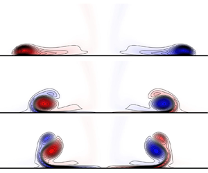
In this study we examine both the head-on and highly inclined oblique interactions between a vortex ring and partial-slip walls with various slip coefficients. For the head-on collision, the quantity of secondary vorticity diffused into the fluid increases as the slip coefficient decreases, leading to a stronger secondary vortex, and therefore, increased rebound of the primary vortex ring. For the highly inclined oblique interaction, the extent of vortex ring connection to the boundary increases as the slip length increases. No connection to the boundary occurs for the no-slip boundary and the maximum extent of connection occurs for the free-slip boundary.
The structure of this section is as follows. First, in § 3.1 we discuss the problem set-up and numerical methodology. Then, in § 3.2 we examine the orthogonal interaction. Finally, the oblique interaction is considered in § 3.3.
3.1. Numerical set-up
The flow configuration under consideration is as shown in figure 2. A vortex ring with initial circulation  $\varGamma _0$, ring radius $R_0$ and core radius $a_0$ is situated at a height $H_0$ above the partial-slip wall, and is inclined an angle $\theta _0$ with respect to the wall. We assume the initial vorticity distribution within the vortex ring core is Gaussian, following previous numerical studies (Zhang et al. Reference Zhang, Shen and Yue1999; Terrington et al. Reference Terrington, Hourigan and Thompson2022a),
 \begin{equation} \omega_{axial} = \frac{\varGamma_0}{{\rm \pi} a_0^2} \exp \left( -\frac{r^2}{a_0^2} \right), \end{equation}
where  $\omega _{axial}$ is the component of vorticity aligned with the vortex core axis and $r$ is the distance from the vortex ring core.
Flow configuration investigated in this work. A vortex ring with initial circulation  $\varGamma _0$, ring radius $R_0$ and core radius $a_0$ is positioned at a height $H_0$ above a partial-slip wall, and is inclined at an angle $\theta _0$ with respect to the wall. The computational domain is a rectangular box with dimensions $L_x$, $L_y$ and $L_z$.

The flow is non-dimensionalised by the vortex ring radius  $R_0$, the initial circulation of the vortex ring $\varGamma _0$ and the kinematic viscosity of the fluid $\nu$. Therefore, the flow is characterised by the following non-dimensional parameters: the Reynolds number $Re = \varGamma _0/\nu$, the slip coefficient $\alpha = (\lambda /R_0)/(1+\lambda /R_0)$, the core-diameter ratio $a_0/R_0$, the depth ratio $H_0/R_0$ and the inclination $\theta _0$. The main focus of this investigation is the slip coefficient, and therefore, all other parameters are held constant. For the orthogonal interaction ( $\theta _0 = 0^\circ$), we consider $Re = 1743$, $a_0/R_0 = 0.4$ and $H_0/R_0 = 3$ for comparison with data from Chu et al. (Reference Chu, Wang and Chang1995a), while for the oblique interaction, we consider $\theta _0 = 80^\circ$, $Re = 1570$, $a_0/R_0 = 0.35$ and $H_0/R_0 = 2.5$, to compare our results with Terrington et al. (Reference Terrington, Hourigan and Thompson2022a).
Numerical simulations were performed using the open-source software package foam-extend 4.1, which is a fork of the OpenFOAM software. Foam-extend 4.1 was previously used to simulate the related problem of a vortex ring interacting with a deformable free surface (Terrington et al. Reference Terrington, Hourigan and Thompson2022a). In the present study we use the pimpleFoam solver implemented in foam-extend 4.1. In this solver, pressure–velocity coupling is achieved using the PIMPLE algorithm, which combines the PISO (Issa Reference Issa1986) and SIMPLE (Patankar & Spalding Reference Patankar and Spalding1972) algorithms. The continuity and momentum equations ((2.2) and (2.1)) are discretised using the finite volume method. Gaussian finite volume integration was used for all spatial derivatives, with second-order linear interpolation for all terms aside from the advection term, which uses the second-order linear-upwind interpolation. Time is discretised using a second-order backwards scheme.
As shown in figure 2, the semi-infinite domain is truncated to lengths of  $L_x$, $L_y$ and $L_z$ in the $x$,
$x$,  $y$ and $z$ directions, respectively. For the orthogonal-interaction case, we use $L_x = L_y = 20$ and $L_z = 10$, which are sufficiently large as to not introduce significant domain blockage effects (Cheng et al. Reference Cheng, Lou and Luo2010). The upper boundary ( $z = L_z$) was set to a free-slip boundary, while the remaining far-field boundaries (at $x = \pm\, L_x/2$ and $y = \pm\, L_y/2$) were set to constant pressure outlets. For the oblique interaction, we used $L_x = L_y = L_z = 10$, which is larger than the domain considered by Zhang et al. (Reference Zhang, Shen and Yue1999). The upper boundary $z = L_z$ was set to a free-slip boundary, the side boundaries $y = \pm\, L_y/2$ were set to symmetry planes and periodic boundary conditions were applied at $x = \pm\, L_x/2$. The computational domain was meshed with a block-structured mesh using the blockMesh utility in foam-extend 4.1.
For the orthogonal interaction, we perform a mesh resolution and validation study by comparing with experimental and numerical data from Chu et al. (Reference Chu, Wang and Chang1995a) for the no-slip case ( $\alpha = 0$). Three meshes with increasing resolution were used, as listed in table 1. We performed two sets of simulations. The first uses $a_0/R_0 = 0.21$, to match the parameters used by Chu et al. (Reference Chu, Wang and Chang1995a). As shown in figure 3(a), which plots the trajectory of the vortex ring core, this first set of simulations is in good agreement with the numerical data of Chu et al. (Reference Chu, Wang and Chang1995a) and reasonable agreement with the experimental data. However, as shown in figure 3(b), the maximum vorticity magnitude is not as well resolved. In particular, the initial vorticity magnitude does not match the initial condition $\omega _0 = \varGamma _0/({\rm \pi} a_0)$. Therefore, mesh 3 is too coarse to resolve the initial core radius of $a_0/R_0 = 0.21$. A second set of simulations was performed with a larger initial core radius of $a_0/R_0 = 0.4$. While the vortex ring trajectory now differs from Chu et al. (Reference Chu, Wang and Chang1995a), due to the change in the initial core radius, changes in both the vortex ring trajectory and the maximum vorticity magnitude between meshes $2$ and $3$ are small. Therefore, $a_0/R_0 = 0.4$ was used for this study, and mesh 2 is considered satisfactory.
Numerical grids used for the orthogonal case ( $\theta _0 = 0^\circ$). Here $N$ is the total number of cells, while $\Delta x$, $\Delta y$ and $\Delta z$ indicate representative cell spacings near the vortex ring. Spacing in the $z$ direction is provided at both the partial-slip wall ( $\Delta z_{0}$) and at $z = 4$ ( $\Delta z_{4}$).

Grid resolution and validation study for the orthogonal interaction between a vortex ring and a no-slip wall, showing (a) the trajectories of the vortex core, and (b) the time histories of the maximum vorticity magnitude, normalised by the initial maximum vorticity  $\omega _0 = \varGamma _0/({\rm \pi} a_0^2)$. Two different initial core radii are considered, $a_0/R_0 = 0.21$ and $a_0/R_0 = 0.4$. Numerical and experimental data from Chu et al. (Reference Chu, Wang and Chang1995a) are also shown in (a). Physical parameters are $\theta = 0$, $Re = 1743$ and $H_0/R_0 = 3$.

For the oblique case, a mesh resolution study was performed at  $\alpha = 1$ (free slip), with parameters matching our previous numerical study of the interaction between a vortex ring and a free surface (Terrington et al. Reference Terrington, Hourigan and Thompson2022a). Three meshes were used, as listed in table 2. Figure 4 plots the maximum spanwise vorticity in the symmetry plane, as well as the maximum vorticity magnitude at the free-slip wall, for each of the three meshes. The change in the solution between meshes $2$ and $3$ is small, and therefore, mesh $3$ is considered converged. The solution obtained for the interaction between a vortex ring and a free surface (Terrington et al. Reference Terrington, Hourigan and Thompson2022a), at $Fr = 0.01$ (i.e. nearly flat), is also shown, and good agreement is observed. The slight differences in solution are likely due to the lack of a periodic domain in Terrington et al. (Reference Terrington, Hourigan and Thompson2022a), and the different domain size between the two studies.
Numerical grids used for the oblique case ( $\theta _0 = 80^\circ$). Here $N$ is the total number of cells, while $\Delta x$, $\Delta y$ and $\Delta z$ indicate the cell spacings near the vortex ring. Spacing in the $z$ direction is provided at both the partial-slip wall ( $\Delta z_{0}$) and at $z = 4$ ( $\Delta z_{4}$).

Resolution study for the oblique interaction between a vortex ring and a free-slip boundary, showing the maximum magnitude of vorticity in both the symmetry plane and the free-slip boundary, for  $\theta = 80^\circ$, $Re = 1570$, $a_0/R_0 = 0.35$ and $H_0/R_0 = 2.5$. Numerical data from Terrington et al. (Reference Terrington, Hourigan and Thompson2022a) for the interaction between a vortex ring and a free surface with $Fr = 0.01$ are also provided.

3.2. Orthogonal interaction
This section considers the head-on collision between a vortex ring and a partial-slip wall ( $\theta _0 = 0$). Contours of spanwise vorticity ( $\omega _y$) in the $x$–
$x$– $z$ plane, overlaid with velocity vectors, are presented in figure 5 for a free-slip boundary ( $\alpha = 1$), in figure 6 for a no-slip boundary ( $\alpha = 0$) and in figure 7 for partial-slip boundaries with $\alpha = 0.5$ (a,b), $\alpha = 0.25$ (c,d) and $\alpha = 0.1$ (e, f). A transient animation comparing the vorticity contours for four different slip coefficients ( $\alpha = 1, 0.25, 0.1, 0$) is also provided in supplementary movie 1 available at https://doi.org/10.1017/jfm.2024.68.
Contour plots of vorticity in the plane  $y = 0$ overlaid with velocity vectors for the interaction between a vortex ring and a free-slip wall ( $\alpha = 1$). The contour levels are $\omega _y = \ldots,-0.3,-0.1,0.1,0.3,\ldots$.

Contour plots of vorticity in the plane  $y = 0$ overlaid with velocity vectors, for the interaction between a vortex ring and a no-slip wall ( $\alpha = 0$). The contour levels are $\omega _y = \ldots,-0.3,-0.1,0.1,0.3,\ldots$.

Contour plots of vorticity in the plane  $y = 0$ overlaid with velocity vectors, for the interaction between a vortex ring and a partial-slip wall with $\alpha = 0.5$ (a,b), $\alpha = 0.25$ (c,d) and $\alpha = 0.1$ (e, f). The contour levels are $\omega _y = \ldots,-0.3,-0.1,0.1,0.3,\ldots$.

The free-slip case is shown in figure 5. This case exhibits three distinct stages of motion, as recognised by Chu et al. (Reference Chu, Wang, Chang, Chang and Chang1995b) for the mathematically equivalent problem of the head-on collision between two identical vortex rings. First, in the free-travelling stage, the vortex ring initially approaches the wall under its own self-induced velocity, where it is deflected and travels radially outwards along the wall. Next, in the vortex stretching stage, strong vortex stretching results in a reduction in the vortex ring core radius, and an increase in the maximum vorticity magnitude (figure 5c). As discussed by Orlandi & Verzicco (Reference Orlandi and Verzicco1993), the vortex ring core forms a head–tail structure during this stage of the interaction. Finally, in the viscous dissipation stage, large vorticity gradients near the boundary lead to the diffusion of vorticity out of the fluid, resulting in a reduction in the peak vorticity magnitude in the vortex ring core (figure 5d).
For the no-slip case (figure 6), the flow is modified by the generation of secondary vorticity at the boundary. As discussed by Cheng et al. (Reference Cheng, Lou and Luo2010), secondary vorticity of sign opposite to the primary vortex ring is generated at the boundary. As the primary vortex ring interacts with this boundary layer, it draws vorticity away from the wall, forming a secondary vortex (figure 6b). The interaction between the primary and secondary vortices then lifts the primary vortex away from the wall, in a process known as rebound (Lim et al. Reference Lim, Nickels and Chong1991). The removal of vorticity from the boundary layer by the primary vortex ring also reduces the tangential motion of the vortex ring along the boundary (Orlandi & Verzicco Reference Orlandi and Verzicco1993). Finally, a second interaction between the primary vortex ring and the wall produces an additional tertiary vortex ring (figure 6d).
The partial-slip cases exhibit behaviour intermediate between the limiting free-slip and no-slip cases. As shown in figure 7, the quantity of secondary vorticity diffused into the fluid increases as the slip coefficient is decreased, with no secondary vorticity created for the free-slip case (figure 5) and the strongest secondary vorticity generated at a no-slip boundary (figure 6). As a result, the quantity of secondary vorticity removed from the boundary layer to form the secondary vortex increases as the slip coefficient is decreased. The increased removal of vorticity from the boundary layer results in a reduction in the radial motion of the vortex ring along the wall.
The increased strength of the secondary vortex also results in a stronger rebound effect. Figure 8(a) plots the trajectories of the primary (solid lines) and secondary (dashed lines) vortex ring cores, which are identified as local maxima in vorticity magnitude. The trajectories of the primary vortex ring for partial-slip boundaries are intermediate between the two limiting cases of no-slip ( $\alpha = 0$) and free-slip ( $\alpha = 1$) boundaries. The distance from the vortex ring to the wall increases as the slip coefficient decreases, due to stronger interactions with the secondary vorticity. No rebound occurs for $\alpha = 1, 0.5$ and $0.25$ (i.e. the distance from the wall decreases monotonically), and the secondary vortex (defined as a local maxima of vorticity magnitude) is either weak or non-existent for these slip lengths. Rebound occurs for $\alpha = 0.1, 0.05$ and $0$, and a stronger secondary vortex is formed for these cases. The strength of the rebound increases as the slip length increases, corresponding to an increase in the strength of the secondary vortex.
Variation in (a) the trajectory of the vortex ring core and (b) the time history of maximum vorticity magnitude, against slip coefficient ( $\alpha$), for both the primary (solid lines) and secondary (dashed lines) vortex rings.

Figure 8(b) presents the maximum azimuthal vorticity for the primary (solid lines) and secondary vortices (dashed lines) for a range of slip coefficients. For the free-slip case ( $\alpha = 1$), the maximum vorticity of the primary vortex nearly doubles as the vortex ring interacts with the wall, due to increased vortex stretching as the vortex ring radius increases (Orlandi & Verzicco Reference Orlandi and Verzicco1993). As $\alpha$ is decreased, the peak value of the maximum vorticity decreases, indicating a reduction in the vortex stretching effect as the radial motion of the vortex ring is reduced by the generation of secondary vorticity.
3.2.1. Mechanism of secondary vorticity creation
To summarise the preceding analysis, the main effect of the slip coefficient is to control the amount of secondary vorticity diffused into the fluid from the boundary, with increased secondary vorticity as the slip coefficient is decreased. This results in an increased rebound, and a reduction in the radial distance travelled along the wall.
We now consider the mechanism responsible for generating the secondary vorticity. Recall that the slip velocity represents a sheet of vector circulation at the partial-slip boundary:
 \begin{equation} \boldsymbol{ \gamma} = \boldsymbol{\hat{e}}_z \times \boldsymbol{u}. \end{equation}
Here  $\boldsymbol {\hat {e}}_z$ is the unit normal vector in the vertical direction. Figure 9 presents a colour-density plot of the magnitude of vector circulation in the interface vortex sheet ( $|\boldsymbol { \gamma }|$), as well as vortex lines in the interface vortex sheet (lines tangent to $\boldsymbol { \gamma }$), at $t = 20$, and for a range of slip coefficients. Transparent isosurfaces of vorticity magnitude are also shown. A transient animation of this figure is also presented in movie 2.
Colour plot showing the magnitude of vector circulation in the interface vortex sheet  $|\boldsymbol {\gamma }|$, as well as vortex lines in the interface vortex sheet, at $t = 20$. Transparent isosurfaces of vorticity magnitude $|\boldsymbol {\omega }| = 0.5$ are also shown, with blue indicating the primary vortex and red indicating the secondary vorticity.

For a free-slip boundary (figure 9a), vector circulation is generated in the interface vortex sheet as the vortex ring approaches the wall, with orientation opposite to that of the primary vortex ring. For partial-slip walls (figure 9b,c), vector circulation is still present in the vortex sheet, however, the strength of the vortex sheet decreases as the slip coefficient is decreased. Finally, there is no interface vortex sheet at the no-slip wall (figure 9d). The reduced strength of the interface vortex sheet corresponds with an increased levels of secondary vorticity, indicating that vector circulation is diffused out of the interface vortex sheet and into the fluid.
To examine the creation of the interface vortex sheet, as well as the secondary vorticity, we consider the reference surface  $S$ shown in figure 10. The boundary curve of this surface is split into two portions: the curve $C_f$ is in the fluid interior, while $C_s$ lies on the partial-slip wall. The total circulation ( $\varGamma$) is expressed as
 $$\begin{gather} \varGamma = \varGamma_\omega + \varGamma_\gamma, \end{gather}$$
 $$\begin{gather}\varGamma_\omega = \int_S \omega \boldsymbol{\cdot} \mathrm d \boldsymbol{S} = \oint_{C_s + C_f} \boldsymbol{u} \boldsymbol{\cdot} \mathrm d \boldsymbol{s}, \end{gather}$$
 $$\begin{gather}\varGamma_\gamma = \int_{C_s} - \boldsymbol{u} \boldsymbol{\cdot} \mathrm d \boldsymbol{s}, \end{gather}$$
and includes contributions from vorticity in the fluid interior ( $\varGamma _\omega$) and circulation in the interface vortex sheet ( $\varGamma _\gamma$). The orientation of $S$ is such that the circulation due to the primary vortex ring is positive.
Control surface  $S$ and boundary curve $C$ for computing the circulation balance. Here $C_s$ is the portion of $C$ on the boundary, while $C_f$ is the remaining portion that lies in the fluid interior.

Using (2.40), (2.49), (2.50) from Terrington et al. (Reference Terrington, Hourigan and Thompson2022b), the rates of change of  $\varGamma$, $\varGamma _\omega$ and $\varGamma _\gamma$ are given by
 $$\begin{gather} \frac{\mathrm d \varGamma}{\mathrm d t} = [p_b - p_a], \end{gather}$$
 $$\begin{gather}\frac{\mathrm d \varGamma_\omega}{\mathrm d t} = \int_{C_s} \left[ \frac{1}{Re} \boldsymbol{\hat{s}} \times(\boldsymbol{\nabla} \times \boldsymbol{ \omega} )\right] \boldsymbol{\cdot} \boldsymbol{\hat{n}}\, \mathrm d s, \end{gather}$$
 $$\begin{gather}\frac{\mathrm d \varGamma_\gamma}{\mathrm d t} = [p_b - p_a] - \int_{C_s} \left[ \frac{1}{Re} \boldsymbol{\hat{s}} \times(\boldsymbol{\nabla} \times \boldsymbol{ \omega} )\right] \boldsymbol{\cdot} \boldsymbol{\hat{n}}\, \mathrm d s, \end{gather}$$
where  $\boldsymbol {\hat {n}}$ is the unit normal to $S$, and we have assumed all fluxes of vorticity across $C_f$ are negligible. Since the partial-slip wall is held stationary, a net change in the total circulation can only be generated by tangential pressure gradients. These pressure gradients accelerate the fluid with respect to the wall, generating circulation in the interface vortex sheet. The viscous boundary flux $({1}/{Re}) \boldsymbol {\hat {s}} \times (\boldsymbol {\nabla } \times \boldsymbol { \omega })$ transfers circulation between the interface vortex sheet and the fluid interior, in order to maintain the partial-slip boundary condition, without generating a net circulation.
Figure 11 presents time histories of  $\varGamma$ (solid lines), $\varGamma _\omega$ (dashed lines) and $\varGamma _\gamma$ (dash-dotted lines) for a range of slip coefficients, while figure 12 presents the rate of change of circulation, as well as the pressure and viscous terms from (3.4), for the free-slip (a), $\alpha = 0.1$ partial-slip (b) and no-slip (c) cases.
Time history of the circulations in the fluid ( $\varGamma _\omega$), interface vortex sheet ( $\varGamma _\gamma$) and the total circulation ( $\varGamma = \varGamma _\omega + \varGamma _\gamma$), for a range of slip coefficients.

Time histories of the rates of change of circulations in the fluid ( $\varGamma _\omega$), interface vortex sheet ( $\varGamma _\gamma$) and total circulation ( $\varGamma _\omega +\varGamma _\gamma$), as well as the viscous and pressure terms from (3.4), for slip coefficients (a) $\alpha = 1$, (b) $\alpha = 0.1$ and (c) $\alpha = 0$.

We first consider the initial approach of the vortex ring to the boundary ( $0< t<20$). As shown in figure 11, the total circulation is approximately independent of slip coefficient during this time interval. Figure 12 confirms that this circulation is generated by tangential pressure gradients at the boundary. To understand the pressure gradients involved, we provide the sketch in figure 13. As the vortex ring approaches the boundary, the velocity field induced by the primary vortex ring features a stagnation point at the symmetry axis, which is a region of high pressure. Fluid at the boundary is accelerated away from the stagnation point, resulting in a slip velocity at the boundary. This is equivalent to a vortex sheet, with orientation opposite to that of the primary vortex ring.
Sketch of the general vorticity creation mechanism. The vortex ring induces a tangential velocity at the boundary, thereby creating an interface vortex sheet. Depending on the slip coefficient, the boundary vorticity flux transfers vorticity into the fluid interior to satisfy the partial-slip boundary condition.

While the slip coefficient does not affect the generation of circulation, it governs how circulation is redistributed between the interface vortex sheet and the fluid interior. The partial-slip boundary condition (2.25) provides the following relationship between the boundary vorticity and the strength of the interface vortex sheet:
 \begin{equation} \alpha \boldsymbol{ \omega}_{{\parallel}} = (1-\alpha)\boldsymbol{ \gamma}.\end{equation}
Circulation is transferred between the interface vortex sheet and the fluid interior to maintain this condition. As the slip coefficient is decreased, the ratio of interface circulation to boundary vorticity decreases and, therefore, a greater quantity of circulation is diffused into the fluid as secondary vorticity.
For the free-slip case, the partial-slip boundary condition is  $\boldsymbol { \omega }_\parallel = \boldsymbol {0}$, and therefore, no secondary vorticity is diffused into the fluid. Referring to figure 11, the circulation in the fluid ( $\varGamma _\omega$) remains constant for $0< t<20$, while a negative circulation is generated in the interface vortex sheet. As shown in figure 12(a), the pressure gradient generates the negative circulation in the interface vortex sheet, and there is no viscous flux of vorticity into the fluid.
For  $t>20$, the primary vortex ring interacts with the boundary. To maintain $\boldsymbol { \omega }_\parallel = \boldsymbol {0}$ on the boundary, vorticity from the primary vortex ring is diffused out of the fluid and into the interface vortex sheet, as indicated by the viscous flux term in figure 12(a). This produces equal and opposite changes to the circulations $\varGamma _\omega$ and $\varGamma _\gamma$. Both the magnitude of positive $\varGamma _\omega$ and the magnitude of negative $\varGamma _\gamma$ decrease by an equal amount, without affecting the total circulation (figure 11).
For the no-slip boundary, the partial-slip boundary condition reduces to  $\boldsymbol { \gamma } = \boldsymbol {0}$. Therefore, all circulation generated by tangential pressure gradients is diffused into the fluid as secondary vorticity. Referring to figure 11, $\varGamma _\gamma$ remains equal to zero, while $\varGamma _\omega$ decreases due to the creation of negative secondary vorticity. As shown in figure 12(c), the pressure gradient and viscous flux terms are equal (aside from small numerical errors in computing the vorticity gradients), and therefore, all circulation generated by the tangential pressure gradient is immediately diffused into the fluid as secondary vorticity.
For partial-slip boundaries, both secondary vorticity and interface circulation must exist at the boundary. Therefore, some circulation is diffused into the fluid, while the rest remains in the interface vortex sheet. As shown in figure 12(b), the viscous flux is less than the pressure-gradient term over the interval  $0< t<20$, and therefore, only a part of the circulation generated by the tangential pressure gradient is diffused into the fluid as secondary vorticity. As shown in figure 11, the amount of circulation diffused into the fluid increases as the slip coefficient is decreased. This is due to the partial-slip boundary condition (3.5), which requires a greater ratio of boundary vorticity to interface circulation as $\alpha$ is decreased.
For  $t>20$, the pressure-gradient term is small (figure 12b), and therefore, the total circulation remains relatively constant. However, the viscous flux remains significant, transferring circulation out of the interface vortex sheet and into the fluid. As shown in figure 7, the primary vortex ring interacts with the boundary vorticity, both drawing positive vorticity away from the boundary, as well as reducing the magnitude of boundary vorticity by the viscous cross-annihilation of opposite-signed vorticity. Therefore, new vorticity must be added at the boundary by the viscous flux to maintain the partial-slip boundary condition.
3.3. Oblique interaction
We now consider the oblique interaction ( $\theta _0 = 80^\circ$). Figures 14–17 present three- dimensional visualisations of the interaction between a vortex ring and a partial-slip boundary, with slip coefficients of $\alpha = 1$ (figure 14), $\alpha = 0.25$ (figure 15), $\alpha = 0.1$ (figure 16) and $\alpha = 0$ (figure 17). In each of these figures, (a–c) plot isosurfaces of vorticity magnitude ( $|\omega | = 0.5$), vortex lines in the fluid and a colour-density plot of surface-normal vorticity ( $\omega _z$) at the partial-slip wall. Subfigures (d–f) present a colour-density plot of the magnitude of vector circulation in the interface vortex sheet ( $|\boldsymbol { \gamma }|$), vortex lines in the interface vortex sheet (i.e. curves tangent to $\boldsymbol { \gamma }$) and transparent vorticity magnitude isosurfaces. A transient animation of these figures is provided in supplementary movie 3.
Interaction between a vortex ring and a free-slip wall ( $\alpha = 1$). Subfigures (a–c) present isosurfaces of vorticity magnitude $|\boldsymbol { \omega }| = 0.5$, vortex lines in the fluid and a colour-density plot of surface-normal vorticity $\omega _z$ at the boundary. Subfigures (d–f) present a colour plot of the strength of the interface vortex sheet $|\boldsymbol { \gamma }|$ and vortex lines in the interface vortex sheet (curves tangent to $\boldsymbol { \gamma }$), overlaid with a transparent isosurface of vorticity magnitude.

Interaction between a vortex ring and a partial-slip wall, with  $\alpha = 0.25$. Subfigures (a–f) are as labelled in figure 14.

Interaction between a vortex ring and a partial-slip wall, with  $\alpha = 0.1$. Subfigures (a–f) are as labelled in figure 14.

Interaction between a vortex ring and a no-slip wall ( $\alpha = 0$). Subfigures (a–f) are as labelled in figure 14.

We also present contour plots of spanwise vorticity ( $\omega _y$) in the symmetry plane ( $y = 0$), overlaid with velocity vectors, in figures 18 and 19 for $\alpha = 1$ (figure 18a–c), $\alpha = 0.25$ (figure 18d–f), $\alpha = 0.1$ (figure 19a–c) and $\alpha = 0$ (figure 19d–f). A transient animation of these figures is also provided in supplementary movie 4.
Contours of spanwise vorticity ( $\omega _y$) in the symmetry plane ( $y = 0$), overlaid with velocity vectors, for slip coefficients (a–c) $\alpha = 1$ and (d–f) $\alpha = 0.25$. The contour levels are $\omega _y = \ldots,-0.3,-0.1,0.1,0.3,\ldots$.

Contours of spanwise vorticity ( $\omega _y$) in the symmetry plane ( $y = 0$), overlaid with velocity vectors, for slip coefficients (a–c) $\alpha = 0.1$ and (d–f) $\alpha = 0$. The contour levels are $\omega _y = \ldots,-0.3,-0.1,0.1,0.3,\ldots$.

We begin by considering the free-slip case ( $\alpha = 1$). The main feature of the interaction is that the vortex ring opens up and attaches to the boundary (Bernal & Kwon Reference Bernal and Kwon1989; Terrington et al. Reference Terrington, Hourigan and Thompson2022a). Initially, the vortex ring is a closed loop (figure 14a). The upper part of the vortex ring corresponds with negative spanwise vorticity in figure 18(a), while the lower part of the vortex ring corresponds with positive spanwise vorticity. As the vortex ring interacts with the free-slip boundary, vortex lines open up and attach to the boundary (figure 14b,c). The opening up of vortex lines corresponds with the loss of positive spanwise vorticity from the symmetry plane, as seen in figure 18(b,c), while the attachment of vortex lines to the boundary corresponds with the appearance of surface-normal vorticity $\omega _z$ at the boundary (figure 14c).
The free-slip case is mathematically equivalent to the oblique interaction between two identical vortex rings studied by Kida et al. (Reference Kida, Takaoka and Hussain1991). Many flow features are identical between both cases, including the flattening of the vortex ring core near the boundary/symmetry plane (figure 14b), the breaking open of vortex lines (figure 14c), and a small ‘thread’ of non-reconnected vorticity remaining after the interaction (figure 14c). The attachment of vortex lines to the surface observed here corresponds to the reconnection of the two vortex rings in Reference Kida, Takaoka and HussainKida et al.'s (Reference Kida, Takaoka and Hussain1991) study.
We now consider the interface vortex sheet. As shown in figure 14(d), vector circulation is generated in the interface vortex sheet as the vortex ring approaches the boundary. The initial vortex sheet comprises two sets of closed-loop vortex lines. As the vortex ring interacts with the free-slip boundary, positive spanwise vorticity ( $\omega _y$) is diffused out of the fluid and into the interface vortex sheet. Therefore, in the final state the interface vortex sheet primarily contains positive spanwise-oriented vector circulation (figure 14f). Moreover, according to (2.26), vortex lines in the interface vortex sheet begin and end at regions of positive and negative vertical vorticity ( $\omega _z$), respectively. Therefore, after the vortex ring has attached to the boundary, vortex lines in the interface vortex sheet begin and end at the locations where the ends of the vortex ring are attached to the boundary (figure 14c, f). Effectively, the vortex ring remains a closed loop, with the lower part of the vortex ring having been diffused out of the fluid, and into the interface vortex sheet (Terrington et al. Reference Terrington, Hourigan and Thompson2022a).
We now consider the no-slip case,  $\alpha = 0$. The no-slip boundary cannot sustain an interface vortex sheet, and therefore, $\boldsymbol { \gamma } = 0$ (figure 17d–f). Any vector circulation generated at the boundary by tangential pressure gradients is immediately diffused into the fluid as secondary vorticity. Secondary vorticity is clearly evident in figure 17(a), and comprises two sets of closed loops. The closed loops of secondary vorticity are qualitatively similar to the closed loops of vector circulation in the interface vortex sheet generated for the free-slip case (figure 14d). This suggests that the pressure gradients during the initial approach of the vortex ring are relatively independent of the slip length. While the generated vector circulation remains in the interface vortex sheet for the free-surface case, it is instead diffused into the fluid as secondary vorticity for the no-slip case. The generated secondary vorticity is also clearly evident in the contours of spanwise vorticity presented in figure 19(d). Negative secondary vorticity is generated directly beneath the vortex ring, while positive vorticity is generated both upstream and downstream of the vortex ring. These regions of positive and negative secondary vorticity correspond to where the loop-shaped vortex lines intersect the symmetry plane.
There is no vortex reconnection to the boundary for the no-slip case. Instead, the lower part of the vortex ring interacts with the secondary vorticity. During the initial stages of this interaction (figure 17b), vortex lines in the lower part of the vortex ring open up and connect with vortex lines in the secondary vorticity. This produces a single set of closed vortex lines (figure 17c), with no clear distinction between primary and secondary vorticity. Referring to the contours of spanwise vorticity (figure 19b,c), the lower part of the vortex ring merges with the secondary vorticity. The small amount of negative secondary vorticity is annihilated by the much larger quantity of positive vorticity, leaving only positive vorticity. This positive vorticity remains in the fluid, and does not diffuse out of the boundary.
We now consider the partial-slip cases, which exhibit behaviour intermediate between the limiting cases of no-slip and free-slip boundaries. We consider two main flow features. First, the amount of secondary vorticity diffused into the fluid increases as the slip length is decreased. Second, the extent of vortex connection to the boundary increases as the slip length is increased. We now discuss these two observations using our theoretical formulation of vorticity dynamics.
3.3.1. Generation of secondary vorticity
The amount of secondary vorticity diffused into the fluid increases as the slip length is decreased, as is clearly evident by comparing figures 18(a,d) and 19(a,d). No secondary vorticity appears for the free-slip case ( $\alpha = 1$), while a small amount of secondary vorticity appears for $\alpha = 0.25$. The amount of secondary vorticity increases as $\alpha$ is decreased further to $\alpha = 0.1$, and the maximum quantity of secondary vorticity is generated for the no-slip case ( $\alpha = 0$).
The appearance of secondary vorticity in the fluid coincides with a reduction in the strength of the interface vortex sheet. The free-slip boundary has the strongest vortex sheet (figure 17d), and the strength of the vortex sheet decreases as the slip length is reduced (figures 15d and 16d). Finally, no vortex sheet is present at the no-slip boundary (figure 17d).
These observations are readily understood under the inviscid model of vector circulation generation. The creation of vector circulation at the boundary is due to tangential pressure gradients, which produce an inviscid relative acceleration between the fluid and the boundary. In figure 20 we plot contours of surface pressure at  $t = 20$ for both the free-slip ( $\alpha = 1$) and no-slip ( $\alpha = 0$) boundaries. The pressure profiles are relatively insensitive to slip coefficient, with only a small difference in the magnitude of the pressure peaks, and therefore, the distribution of vector circulation generated at the boundary does not significantly depend on the slip coefficient. Fluid at the boundary is accelerated away from the positive upstream pressure peak and towards the negative downstream pressure peak.
Contours of pressure on the boundary for (a)  $\alpha = 1$ and (b) $\alpha = 0$, at $t = 20$. Transparent isosurfaces of $|\boldsymbol { \omega } | = 0.5$ are also shown for reference.

The interface vortex sheet can also be interpreted as a consequence of the tangential velocity induced by the primary vortex ring, as shown in figure 21. Directly below the vortex ring, the induced tangential velocity is negative, indicating that negative vector circulation is generated there. Both ahead of the upstream stagnation point and behind the downstream stagnation point, the induced tangential velocity is positive, indicating positive vector circulation. Considering the full three-dimensional flow (figure 21b), fluid is accelerated away from the upstream stagnation point (due to the positive pressure) and towards the downstream stagnation point (due to the negative pressure), resulting in two sets of closed loops of vector circulation. This matches the closed loops of vector circulation in the interface vortex sheet at a free-slip boundary (figure 14d) and the closed loops of secondary vorticity at the no-slip boundary (figure 17a).
Sketch illustrating the generation of vector circulation in the interface vortex sheet. The approaching vortex ring induces a tangential velocity at the boundary, thereby creating a vortex sheet.

While the slip coefficient does not affect the generation of vector circulation, it determines how vector circulation is distributed between the interface vortex sheet and the fluid. The partial-slip boundary condition prescribes the ratio between vector circulation in the interface vortex sheet and boundary vorticity:  $\alpha \boldsymbol { \omega }_\parallel = (1-\alpha ) \boldsymbol { \gamma }$. For the free-slip boundary, this becomes $\boldsymbol { \omega }_\parallel = \boldsymbol {0}$, and all vector circulation remains in the interface vortex sheet. For the no-slip boundary, we have $\boldsymbol { \gamma } =\boldsymbol {0}$ and all vector circulation is diffused into the fluid as secondary vorticity. For the partial-slip boundary, both boundary vorticity and the interface vortex sheet must exist simultaneously. As $\alpha$ is increased, a greater quantity of vector circulation must remain in the interface vortex sheet, and therefore, less secondary vorticity is diffused into the fluid.
3.3.2. Extent of vortex ring connection to the boundary
The extent of vortex ring connection to the boundary also depends on the slip coefficient. For the free-slip case (figure 14c), most of the vortex lines open up and attach to the boundary, and this is accompanied by the loss of most of the positive spanwise vorticity from the fluid (figure 18c). For  $\alpha = 0.25$ (figure 15c), the vortex ring opens up and connects to the boundary. However, slightly more positive spanwise vorticity remains in the fluid (figure 18f), indicating a reduced extent of reconnection. For $\alpha = 0.1$ (figure 16c), some vortex lines open up and attach to the boundary, however, many of the vortex lines remain as closed loops. This corresponds with a substantial quantity of positive spanwise vorticity remaining in the fluid (figure 19c). Finally, no vortex connection occurs at the no-slip wall (figure 17c) and all positive spanwise vorticity remains in the fluid (figure 19f).
The dynamics of vortex ring connection to the boundary can be understood using the system of control surfaces shown in figure 22 (Terrington et al. Reference Terrington, Hourigan and Thompson2022a). Here,  $S$ is the symmetry plane, while $I_1$ and $I_2$ are the portions of the partial-slip wall on each side of the symmetry plane. These surfaces share a common boundary at the connection line, $C$. The vortex connection process involves a loss of positive circulation from $S$ (i.e. opening up of vortex lines), and an increase of positive circulation in $I_1$ and of negative circulation in $I_2$, indicating the attachment of vortex lines to the boundary. The magnitudes of positive circulation gained in $I_1$ and of negative circulation gained in $I_2$ are both equal to the magnitude of negative circulation lost from $S$, as a consequence of the kinematic condition that vortex lines do not end in the fluid (Terrington et al. Reference Terrington, Hourigan and Thompson2022a).
Control surface analysis for examining vortex ring connection to the boundary.

In figure 23(a) we plot the time histories of the circulations:  $\varGamma _S$, $\varGamma _{I_1}$ and $\varGamma _{I_2}$, which are the circulations in $S$,
$S$,  $I_1$ and $I_2$, respectively. We also plot $\varGamma _\gamma = \int _C \gamma _y$, which is the circulation contained in the interface vortex sheet, along the connection line $C$. Vortex reconnection to the boundary is associated with a decrease in $\varGamma _S$, indicating the loss of positive spanwise vorticity from the fluid. This is also associated with an equal and opposite change to the circulation $\varGamma _\gamma$, as the vorticity lost from the fluid is transferred into the interface vortex sheet. Finally, there is an equal increase of both positive circulation in $\varGamma _{I_1}$ and of negative circulation in $\varGamma _{I_2}$, indicating the attachment of vortex lines to the boundary.
Time histories of (a) the circulations  $\varGamma _S$, $\varGamma _{I_1}$, $\varGamma _{I_2}$ and $\varGamma _{\gamma }$, and (b) the rate of change of circulations $-\mathrm d \varGamma _S/\mathrm d t = \mathrm d \varGamma _{I_1}/\mathrm d t = - \mathrm d\varGamma _{I_2}/\mathrm d t = \mathrm d \varGamma _{\gamma }/\mathrm d t$, for a range of slip coefficients. The viscous boundary flux $F_\nu$ is also shown in subfigure (b).

The free-slip case ( $\alpha = 1$) has the largest changes to each of the circulations, indicating the greatest extent of vortex connection. The changes to the circulations reduce as $\alpha$ is decreased, indicating that the extent of reconnection is reduced. Finally, the circulations remain constant for the no-slip boundary ( $\alpha = 0$), indicating that vortex connection does not occur.
The rate of change of the circulations  $\varGamma _{S}$, $\varGamma _{I_1}$, $\varGamma _{I_2}$ and $\varGamma _{\gamma }$ are given by (4.11a–e) from Terrington et al. (Reference Terrington, Hourigan and Thompson2022a):
 $$\begin{gather} \frac{\mathrm d \varGamma_S}{\mathrm d t} = \frac{\mathrm d }{\mathrm d t} \int_S \omega_y\, \mathrm d S ={-}F_\nu, \end{gather}$$
 $$\begin{gather}\frac{\mathrm d \varGamma_{I_1}}{\mathrm d t} = \frac{\mathrm d }{\mathrm d t} \int_{I_1} \omega_z\, \mathrm d S = F_\nu, \end{gather}$$
 $$\begin{gather}\frac{\mathrm d \varGamma_{I_2}}{\mathrm d t} = \frac{\mathrm d }{\mathrm d t} \int_{I_2} \omega_z\, \mathrm d S ={-}F_\nu,\end{gather}$$
 $$\begin{gather}\frac{\mathrm d \varGamma_\gamma}{\mathrm d t} = \frac{\mathrm d }{\mathrm d t}\int_C \gamma_y\, \mathrm d s = F_\nu, \end{gather}$$
 $$\begin{gather}F_\nu = \int_C \frac{1}{Re} \left[ \frac{\partial \omega_y}{\partial z}-\frac{\partial \omega_z}{\partial y} \right]\mathrm d s. \end{gather}$$
Importantly, the rates of change of all of the circulations are governed by the viscous flux of vorticity along the connection line,  $F_\nu$. This viscous flux simultaneously describes the diffusion of spanwise vorticity out of the fluid ( $\mathrm d \varGamma _S/\mathrm d t$) and into the interface vortex sheet ( $\mathrm d \varGamma _\gamma /\mathrm d t$), as well as the appearance of positive and negative vorticity in $I_1$ and $I_2$, respectively ( $\mathrm d \varGamma _{I_1}/\mathrm d t$ and $\mathrm d \varGamma _{I_2}/\mathrm d t$). Importantly, this clearly explains why the exact quantity of circulation lost from the symmetry plane is gained in the boundary, which is a necessary consequence of the kinematic condition that vortex lines do not end in the fluid (Terrington et al. Reference Terrington, Hourigan and Thompson2022a).
Figure 23(b) plots the rates of change of circulations ( $-\mathrm d \varGamma _{S}/\mathrm d t = \mathrm d \varGamma _{I_1}/\mathrm d t = \mathrm d \varGamma _\gamma / \mathrm d t = - \mathrm d \varGamma _{I_2}/\mathrm d t$), as well as the viscous flux $F_\nu$, for a range of slip coefficients, confirming that the rate of change of circulations are described by the viscous flux (small numerical errors are present due to the difficulty of accurately computing vorticity gradients, which are third derivatives of velocity). The viscous flux, and the rate of change of circulation, increase as the slip coefficient is increased, resulting in a greater extent of reconnection.
To understand why vortex reconnection depends on the slip coefficient, recall that the viscous flux  $F_\nu$ ensures that the partial-slip condition is satisfied at the boundary. For a free-slip boundary, this condition requires that $\boldsymbol { \omega }_\parallel = \boldsymbol {0}$ on the boundary. As the vortex ring impinges upon the boundary (figure 18b), positive spanwise vorticity is brought near the boundary. Due to the condition $\boldsymbol { \omega }_\parallel = \boldsymbol {0}$ at the boundary, there is a large vorticity gradient $\partial \omega _y/\partial z$ at the boundary, resulting in a large viscous flux of vorticity $F_\nu$. Therefore, positive vorticity is removed from the fluid, and into the vortex sheet, maintaining the free-slip boundary condition at the boundary. The viscous flux $F_\nu$ also results in the appearance of surface-normal vorticity at the boundary, indicating the attachment of the vortex ring to the boundary.
For partial-slip boundaries, some negative spanwise vorticity must remain at the boundary to satisfy the partial-slip boundary condition  $\alpha \boldsymbol { \omega }_\parallel = (1-\alpha ) \boldsymbol { \gamma }$. As the slip coefficient is reduced, a greater quantity of negative vorticity must remain in the fluid, and therefore, less vorticity is diffused out of the fluid by the viscous flux $F_\nu$. This results in a reduced extent of vortex reconnection.
Finally, for the no-slip boundary, no interface vortex sheet can exist ( $\boldsymbol { \gamma } = \boldsymbol {0}$). Therefore, no circulation is diffused out of the fluid and the net viscous flux $F_\nu$ is zero. As a result, reconnection does not occur at a no-slip boundary.
4. Conclusions
We have discussed the generation and transport of vorticity and vector circulation at partial-slip boundaries, using our general formulation of vorticity dynamics (Terrington et al. Reference Terrington, Hourigan and Thompson2022b). The slip velocity at the boundary represents a surface density of vector circulation, i.e. an interface vortex sheet. The total vector circulation, including both the total vorticity of the fluid and vector circulation in the interface vortex sheet, is generally conserved. Specifically, if there is no external acceleration of the solid boundary, and no net external pressure gradient, the total vector circulation will remain constant. Under these conditions, local generation of vector circulation may still occur on a section of the boundary, but this will be balanced by the generation of opposite-signed vector circulation elsewhere.
The creation of vector circulation does not depend on either viscosity or the partial-slip boundary condition. Vector circulation is generated by the inviscid relative acceleration between the fluid and the solid at the boundary, due to either external acceleration of the boundary or a tangential pressure gradient. Vector circulation within the interface vortex sheet may also be amplified and reoriented by the vortex stretching/tilting term.
While the creation of vector circulation does not depend on either viscosity or the no-slip condition, both viscosity and the no-slip condition determine how vector circulation is redistributed between the total vorticity of the fluid and the interface vortex sheet. The partial-slip boundary condition provides a relationship between the density of vector circulation in the interface vortex sheet and the boundary vorticity. The strength of the interface vortex sheet is greater for large slip lengths, while the intensity of boundary vorticity is greater for small slip lengths. Finally, the viscous boundary vorticity flux transfers vector circulation between the interface vortex sheet and the total vorticity of the fluid to maintain the partial-slip boundary condition, but does not generate a net vector circulation.
The interaction between a vortex ring and a partial-slip wall was examined to illustrate various aspects of our formulation. For the orthogonal interaction, vector circulation is generated at the boundary by tangential pressure gradients as the vortex ring approaches the boundary. While the quantity of vector circulation generated does not depend on the slip coefficient, a greater quantity of vector circulation is diffused into the fluid as secondary vorticity when the slip length is reduced. The secondary vorticity subsequently alters the motion of the primary vortex ring, lifting it away from the wall and reducing the radial motion of the vortex ring along the wall.
For the oblique interaction between a vortex ring and a partial-slip wall, the vortex ring opens up and connects to the boundary. Specifically, spanwise vorticity from the lower part of the vortex ring is diffused out of the fluid and into the interface vortex sheet, causing the vortex ring to attach to the boundary. The extent of connection depends on the slip length. As the slip length is decreased, a greater quantity of vorticity must remain in the fluid, in order to satisfy the partial-slip boundary condition, and therefore, the extent of connection is reduced.
Supplementary movies
Supplementary movies are available at https://doi.org/10.1017/jfm.2024.68.
Funding
This work was supported by the Australian Government through the Australian Research Council's Discovery Projects funding scheme (projects DP210100990 and DP190103388), and by computational resources provided by the National Computational Infrastructure and Pawsey Supercomputer Centre (Merit Grant d71) under the National Computational Merit Allocation Scheme.
Declaration of interests
The authors report no conflict of interest.


 Open access