4.1 Necessity

Suppose ${\mathcal G}_1={\mathcal G}(\delta _1, {\mathcal L}_{{\vec {\textbf {a}}}_1}), \dots , {\mathcal G}_{d+1}={\mathcal G}(\delta _{d+1}, {\mathcal L}_{{\vec {\textbf {a}}}_{d+1}})$ are adjacent. We prove the necessary part by contradiction.

Assume condition (a) fails, that is, there exists some $\ell _1, \ell _2 \in \{1, \dots , d+1\}$ with $\ell _1 \neq \ell _2$ and $s \in \{1, \dots , d\}$ , such that for each $N_1 \ge 1$ , there exists some $m_1 \ge 0$ and $K \in \mathbb {Z}$ , such that

$$ \begin{align*}\left| \left(\delta_{\ell_1} \right)_s-\left(\delta_{\ell_2} \right)_s- \frac{K}{n^{m_1}}\right|< \frac{1}{N_1 n^{m_1}}, \end{align*} $$

which implies that the distance between the hyperplane $\left \{(x)_s=(\delta _{\ell _1})_s\right \}$ and the hyperplane $\left \{(x)_s=(\delta _{\ell _2})_s+K/n^{m_1}\right \}$ is less than $1/(N_1 n^{m_1})$ . On the other hand, note that

$$ \begin{align*}\left\{(x)_s=(\delta_{\ell_1})_s\right\} \subset b\left[ {\mathcal G}_{\ell_1, {m_1}} \right] \end{align*} $$

and

$$ \begin{align*}\left\{(x)_s=(\delta_{\ell_2})_s+\frac{K}{n^{m_1}}\right\} \subset b\left[ {\mathcal G}_{\ell_2, {m_1}} \right], \end{align*} $$

where $b\left [ {\mathcal G}_{\ell _1, m_1} \right ]$ is the union of all the boundaries of the cubes in ${\mathcal G}_{\ell _1}$ with sidelength $1/n^{m_1}$ , and similarly for the term $b\left [ {\mathcal G}_{\ell _2, m_1} \right ]$ .

Now, the idea is to find two sufficiently closed points on the intersection of the boundaries of these n-adic grids. Without loss of generality, let us assume $s=\ell _1=1$ and $\ell _2=2$ . Now, let us consider the points

$$ \begin{align*}p_1:=\{(x)_1=(\delta_1)_1\} \cap \{(x)_2=(\delta_3)_2 \} \cap \cdots \cap \{(x)_d=(\delta_{d+1})_d \} \end{align*} $$

and

$$ \begin{align*}p_2:=\left\{(x)_1=(\delta_2)_1+\frac{K}{n^{m_1}}\right\} \cap \{(x)_2=(\delta_3)_2 \} \cap \cdots \cap \{(x)_d=(\delta_{d+1})_d \} \}, \end{align*} $$

which satisfy the following properties:

1. (a) $p_1 \in b\left [ {\mathcal G}_{1, m_1} \right ] \cap \bigcap \limits _{t=3}^{d+1} b\left [ {\mathcal G}_{t, m_1} \right ]$ and $p_2 \in \bigcap \limits _{t=2}^{d+1} b\left [ {\mathcal G}_{t, m_1} \right ]$ .

2. (b) $\textrm {dist}(p_1, p_2)=\left | \left (\delta _1 \right )_1-\left (\delta _2 \right )_1- K/n^m\right |< 1/(N_1 n^{m_1})$ .

Note that property (b) above allows us to choose an open cube Q of radius $1/(N_1 n^{m_1})$ that containing both $p_1$ and $p_2$ , whereas property (a) asserts that if there is a dyadic cube $D \in {\mathcal G}_{\ell }, \ell \in \{1, \dots , d+1\}$ covering Q, then $\ell (D)>1/n^{m_1}$ , and hence

$$ \begin{align*}\ell(D)>N_1 \ell(Q). \end{align*} $$

This will contradict to the second condition in Definition 1.3 if we choose $N_1$ sufficiently large (see Figure 1).

Figure 1:

$p_1$ , $p_2$ , the hyperplane $\{(x)_1=(\delta _1)_1\}$ (red part), the hyperplane $\left \{(x)_1=(\delta _2)_1+K/n^{m_1}\right \}$ (blue part), the line $L:=\{(x)_2=(\delta _3)_2 \} \cap \cdots \cap \{(x)_d=(\delta _{d+1})_d \}$ , and the cube Q containing both $p_1$ and $p_2$ .

Next, expecting a contradiction again, we assume (b) fails. The proof for this part is very similar to the previous one. Let us consider two different cases.

Case I: There exists some $k_1, k_2 \in \{1, \dots , d+1\}, k_1 \neq k_2$ , and $s \in \{1, \dots , d\}$ , such that

(4.1) $$ \begin{align} \liminf_{j \to \infty} \left|\frac{ \left[{\mathcal L}_{{\vec{\textbf{a}}}_{k_1}}(j)\right]_{s}-\left[{\mathcal L}_{{\vec{\textbf{a}}}_{k_2}}(j)\right]_{s}}{n^j}\right|=0. \end{align} $$

Again, for simplicity, we may assume $s=k_1=1$ and $k_2=2$ . By (4.1), for any $\varepsilon>0$ , there exists some $j_1$ sufficiently large, such that

$$ \begin{align*}\left| \left[{\mathcal L}_{{\vec{\textbf{a}}}_1}(j_1)\right]_1-\left[{\mathcal L}_{{\vec{\textbf{a}}}_2}(j_1)\right]_1 \right|<\varepsilon \cdot n^{j_1}, \end{align*} $$

which implies that

$$ \begin{align*}\left|\left[\delta_1+{\mathcal L}_{{\vec{\textbf{a}}}_1}(j_1)\right]_1-\left[\delta_2+{\mathcal L}_{{\vec{\textbf{a}}}_2}(j_1)\right]_1 \right|<2\varepsilon \cdot n^{j_1}, \end{align*} $$

since we assume $j_1$ is sufficiently large. Now, we can exactly follow the idea in part (a) now. More precisely, we define

$$ \begin{align*}q_1:=\{(x)_1=\left[\delta_1+{\mathcal L}_{{\vec{\textbf{a}}}_1}(j_1)\right]_1\} \cap \bigcup_{t=2}^d \left\{(x)_t=\left[\delta_{t+1}+{\mathcal L}_{{\vec{\textbf{a}}}_{t+1}}(j_1) \right]_t \right\} \end{align*} $$

and

$$ \begin{align*}q_2:= \bigcup_{t=1}^d \left\{(x)_t=\left[\delta_{t+1}+{\mathcal L}_{{\vec{\textbf{a}}}_{t+1}}(j_1) \right]_t \right\}, \end{align*} $$

which enjoy similar properties as $p_1$ and $p_2$ :

1. (a) $q_1 \in b\left [ {\mathcal G}_{1, -j_1} \right ] \cap \bigcap \limits _{k=3}^{d+1} b\left [ {\mathcal G}_{k, -j_1} \right ]$ and $q_2 \in \bigcap \limits _{k=2}^{d+1} b\left [ {\mathcal G}_{k, -j_1} \right ]$ .

2. (b) $\textrm {dist}(q_1, q_2)<2 \varepsilon \cdot n^{j_1}$ .

Then desired contradiction will follow by taking an open cube with sidelength $2\varepsilon \cdot n^{j_1}$ containing both $q_1$ and $q_2$ , where $\varepsilon $ is sufficiently small.

Case II: There exists some $k_1, k_2 \in \{1, \dots , d+1\}, k_1 \neq k_2$ , and $s \in \{1, \dots , d\}$ , such that

(4.2) $$ \begin{align} \limsup_{j \to \infty} \left|\frac{ \left[{\mathcal L}_{{\vec{\textbf{a}}}_{k_1}}(j)\right]_{s}-\left[{\mathcal L}_{{\vec{\textbf{a}}}_{k_2}}(j)\right]_{s}}{n^j}\right|=1. \end{align} $$

The proof for the second case is an easy modification of the first one. Indeed, (4.2) implies that for any $\varepsilon>0$ , there exists some $j_2$ sufficiently large, such that either

$$ \begin{align*}\left| \left[\delta_{k_1}+{\mathcal L}_{{\vec{\textbf{a}}}_{k_1}}(j_2)\right]_{s}-\left[\delta_{k_2}+{\mathcal L}_{{\vec{\textbf{a}}}_{k_2}}(j_2)+n^j \vec{e}_s\right]_{s} \right|<\varepsilon \cdot n^{j_2} \end{align*} $$

or

$$ \begin{align*}\left| \left[\delta_{k_1}+{\mathcal L}_{{\vec{\textbf{a}}}_{k_1}}(j_2)\right]_{s}-\left[\delta_{k_2}+{\mathcal L}_{{\vec{\textbf{a}}}_{k_2}}(j_2)-n^j \vec{e}_s\right]_{s} \right|<\varepsilon \cdot n^{j_2} \end{align*} $$

holds, where in the above estimates, $\vec {e}_s$ refers to the stand unit vector in $\mathbb {R}^d$ with the sth entry being $1$ . The rest of the proof is the same as Case I.

4.2 Sufficiency

Suppose the conditions (a) and (b) hold, that is,

1. (1) For any $\ell _1, \ell _2 \in \{1, \dots , d+1\}$ where $\ell _1 \neq \ell _2$ , and $s \in \{1, \dots , d\}$ , there exists some constant $C(\ell _1, \ell _2, s)>0$ , such that for any $m \ge 0$ and $k \in \mathbb {Z}$ , there holds

   (4.3) $$ \begin{align} \left| \left(\delta_{\ell_1} \right)_s-\left(\delta_{\ell_2} \right)_s- \frac{k}{n^m}\right| \ge \frac{C(\ell_1, \ell_2, s)}{n^m}. \end{align} $$

2. (2) For any $k_1, k_2 \in \{1, \dots , d+1\}, k_1 \neq k_2$ , and $s \in \{1, \dots , d\}$ , there holds

   (4.4) $$ \begin{align} 0< \liminf_{j \to \infty} \left|\frac{ \left[{\mathcal L}_{{\vec{\textbf{a}}}_{k_1}}(j)\right]_{s}-\left[{\mathcal L}_{{\vec{\textbf{a}}}_{k_2}}(j)\right]_{s}}{n^j}\right| \le \limsup_{j \to \infty} \left|\frac{ \left[{\mathcal L}_{{\vec{\textbf{a}}}_{k_1}}(j)\right]_{s}-\left[{\mathcal L}_{{\vec{\textbf{a}}}_{k_2}}(j)\right]_{s}}{n^j}\right|<1. \end{align} $$

Denote

$$ \begin{align*}C_1:=\min_{1 \le \ell_1 \neq \ell_2 \le d+1, 1 \le s \le d} C(\ell_1, \ell_2, s), \quad D_1:=\min_{1 \le k_1 \neq k_2 \le d+1, 1 \le s \le d} D_1(k_1, k_2, s), \end{align*} $$

and

$$ \begin{align*}D_2:=1-\max_{1 \le k_1 \neq k_2 \le d+1, 1 \le s \le d} D_2(k_1, k_2, s), \end{align*} $$

where the quantities $D_1(k_1, k_2, s)$ and $D_2(k_1, k_2, s)$ are defined in Corollary 2.5. Note that $C_1, D_1, D_2>0$ by our assumption (4.4). Moreover, by (4.4), there exists some $N \in {\mathbb N}$ , such that for any $k_1, k_2 \in \{1, \dots , d+1\}, k_1 \neq k_2$ , $s \in \{1, \dots , d\}$ , and $j \ge N$ , there holds

(4.5) $$ \begin{align} \frac{D_1}{2}< \left|\frac{ \left[{\mathcal L}_{{\vec{\textbf{a}}}_{k_1}}(j)\right]_{s}-\left[{\mathcal L}_{{\vec{\textbf{a}}}_{k_2}}(j)\right]_{s}}{n^j}\right|<1-\frac{D_2}{2}. \end{align} $$

Recall that the goal is to show that the collection ${\mathcal G}_1={\mathcal G}(\delta _1, {\mathcal L}_{{\vec {\textbf {a}}}_1}), \dots , {\mathcal G}_{d+1}={\mathcal G}(\delta _{d+1}, {\mathcal L}_{{\vec {\textbf {a}}}_{d+1}})$ is adjacent in $\mathbb {R}^d$ . Take some $C>0$ sufficiently small, such that

$$ \begin{align*}0<C<\min \left\{C_1, \frac{D_1}{4}, \frac{D_2}{4}, \frac{1}{10} \right\}. \end{align*} $$

Now, for any cube Q in $\mathbb {R}^d$ , let $m_0 \in \mathbb {Z}$ such that

$$ \begin{align*}\frac{C}{n^{m_0+1}} \le \ell(Q)<\frac{C}{n^{m_0}}. \end{align*} $$

We consider several cases.

Case I: $m_0>0$ . Let us show that Q is contained in some cube in ${\mathcal G}_{k, m_0}$ for some $k \in \{1, \dots , d+1\}$ . We argue by contradiction. If Q is not contained in any cubes in ${\mathcal G}_{k, m_0}$ for all $k=1, \dots , d+1$ . Then, for each $k \in \{1, \dots , d+1\}$ , there exists some $j_k \in \{1, \dots , d\}$ , such that

$$ \begin{align*}P_{j_k} (Q) \cap P_{j_k} ({\mathcal A}_{k, m_0}) \neq \emptyset, \end{align*} $$

where we recall ${\mathcal A}_{k, m_0}$ is the collection of all the vertices of the cubes in ${\mathcal G}_{k, m_0}$ . By pigeonholing, there exists some $\ell _1, \ell _2 \in \{1, \dots , d+1\}$ with $\ell _1 \neq \ell _2$ , but $j_*:=j_{\ell _1}=j_{\ell _2}$ , such that

$$ \begin{align*}P_{j_*} (Q) \cap P_{j_*} ({\mathcal A}_{\ell_1, m_0}), \quad P_{j_*} (Q) \cap P_{j_*} ({\mathcal A}_{\ell_2, m_0}) \neq \emptyset, \end{align*} $$

which implies that there exists some $K_1, K_2 \in \mathbb {Z}$ , such that

$$ \begin{align*}\left| \left(\delta_{\ell_1}\right)_{j_*}+\frac{K_1}{n^{m_0}} -\left(\delta_{\ell_2} \right)_{j_*}-\frac{K_2}{n^{m_0}} \right| \le \ell(Q)<\frac{C}{n^{m_0}}< \frac{C(\ell_1, \ell_2, j_*)}{n^{m_0}}, \end{align*} $$

which contradicts to (4.3).

Case II: $m_0 \le -N$ . Again, we wish to show that Q is contained in some cubes in ${\mathcal G}_{k, m_0}$ for some $k \in \{1, \dots , d+1\}$ and we prove it by contradiction. Following the argument in Case I above, we see that there exists some $k_1, k_2 \in \{1, \dots , d+1\}$ with $k_1 \neq k_2$ and $j^* \in \{1, \dots , d\}$ , such that

$$ \begin{align*}P_{j^*} (Q) \cap P_{j^*} ({\mathcal A}_{k_1, m_0}), \quad P_{j_*} (Q) \cap P_{j^*} ({\mathcal A}_{k_2, m_0}) \neq \emptyset. \end{align*} $$

This implies that there exists some $K_3, K_4 \in \mathbb {Z}$ , such that

$$ \begin{align*}\left| \left[\delta_{k_1}+{\mathcal L}_{{\vec{\textbf{a}}}_{k_1}}(-m_0) \right]_{j^*}+\frac{K_3}{n^{m_0}}- \left[\delta_{k_2}+{\mathcal L}_{{\vec{\textbf{a}}}_{k_2}}(-m_0) \right]_{j^*}-\frac{K_4}{n^{m_0}} \right|<\frac{C}{n^{m_0}}. \end{align*} $$

Note that since we can always choose N sufficiently large, we can indeed reduce the above estimate to

$$ \begin{align*}\left| \left[{\mathcal L}_{{\vec{\textbf{a}}}_{k_1}}(-m_0) \right]_{j^*}+\frac{K_3}{n^{m_0}}- \left[{\mathcal L}_{{\vec{\textbf{a}}}_{k_2}}(-m_0) \right]_{j^*}-\frac{K_4}{n^{m_0}} \right|<\frac{2C}{n^{m_0}}, \end{align*} $$

which implies that

(4.6) $$ \begin{align} \left| \frac{ \left[{\mathcal L}_{{\vec{\textbf{a}}}_{k_1}}(-m_0) \right]_{j^*}- \left[{\mathcal L}_{{\vec{\textbf{a}}}_{k_2}}(-m_0) \right]_{j^*}}{n^{-m_0}}+(K_3-K_4) \right|< 2C. \end{align} $$

We claim that $K_3-K_4 \in \{-1, 0, 1\}$ . Indeed, by the choice of C, the right-hand side of the above estimate is bounded by $1/5$ ; on the other hand, by the definition of the location function, we have

$$ \begin{align*}\frac{ \left[{\mathcal L}_{{\vec{\textbf{a}}}_{k_1}}(-m_0) \right]_{j^*}- \left[{\mathcal L}_{{\vec{\textbf{a}}}_{k_2}}(-m_0) \right]_{j^*}}{n^{-m_0}} \in (-1, 1). \end{align*} $$

The desired claim then follows from these observations and the fact that $K_3-K_4$ is an integer. Therefore, the estimate (4.6) implies either

$$ \begin{align*}\left| \frac{ \left[{\mathcal L}_{{\vec{\textbf{a}}}_{k_1}}(-m_0) \right]_{j^*}- \left[{\mathcal L}_{{\vec{\textbf{a}}}_{k_2}}(-m_0) \right]_{j^*}}{n^{-m_0}} \right|< 2C<\frac{D_1}{2} \end{align*} $$

or

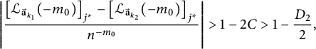$$ \begin{align*}\left| \frac{ \left[{\mathcal L}_{{\vec{\textbf{a}}}_{k_1}}(-m_0) \right]_{j^*}- \left[{\mathcal L}_{{\vec{\textbf{a}}}_{k_2}}(-m_0) \right]_{j^*}}{n^{-m_0}} \right|> 1-2C>1-\frac{D_2}{2}, \end{align*} $$

which contradicts (4.6).

Case III: $-N<m_0 \le 0$ . Indeed, we can “pass” the third case to the second case, by taking a cube $Q'$ containing Q with the sidelength is $n^N$ . Applying the second case to $Q'$ , we find that there exists some $D \in {\mathcal G}_k$ for some $k \in \{1, \dots , d+1\}$ , such that $Q' \subset D$ and $\ell (D) \le C_4 \ell (Q')$ , which clearly implies

1. (1) $Q \subset D$ .

2. (2) $\ell (D) \le C_4 n^N \ell (Q)$ .

The proof is complete.▪

7.1 Corner sets

In the first part of this section, let us introduce an important structure for ${\mathcal G}(\delta , {\mathcal L}_{{\vec {\textbf {a}}}})$ , which can be viewed as a “generator” of ${\mathcal G}(\delta , {\mathcal L}_{{\vec {\textbf {a}}}})$ .

Definition 7.1 Let ${\mathcal G}(\delta , {\mathcal L}_{{\vec {\textbf {a}}}})$ be an n-adic grid in $\mathbb {R}^d$ . For $\ell \in \mathbb {Z}$ , we define the $\ell $ th corner operation

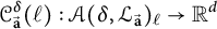$$ \begin{align*}{\mathcal C}_{{\vec{\textbf{a}}}}^{\delta}(\ell) :{\mathcal A}(\delta, {\mathcal L}_{{\vec{\textbf{a}}}})_{\ell} \to \mathbb{R}^d \end{align*} $$

is given by

$$ \begin{align*}\left[{\mathcal C}_{{\vec{\textbf{a}}}}^{\delta}(\ell)\right] (x):= \bigcup_{i=1}^d \prod_i \left(x, \left[(x)_1, (x)_1+n^{-\ell} \right) \times \left[(x)_d, (x)_d+n^{-\ell} \right) \right), \end{align*} $$

where for any $x \in \mathbb {R}^d$ and $A \subset \mathbb {R}^d$ , $\prod _i(x, A)$ denotes the projection of A to the hyperplane $\{y \in \mathbb {R}^d: (y)_i=(x)_i \}$ . We call the collection $\left [{\mathcal C}_{{\vec {\textbf {a}}}}^{\delta }(\ell )\right ] (x)$ the $\ell $ th corner set associated to x with parameters $(\delta , {\vec {\textbf {a}}})$ , and we refer x as the corner of the corner set $\left [{\mathcal C}_{{\vec {\textbf {a}}}}^{\delta } \right ](x)$ .

Below is an example of a corner set with its corner $x = \left (\frac {1}{3}, \frac {1}{3} \right )$ when $d=2, n=2$ , and $\ell =1$ (see Figure 3).

Figure 3:

Corner and corner set.

7.2 Small-scale lattices and $n$ -far vectors

The goal of the second part of section is to generalize the concept of far numbers in one dimension to higher dimension. It turns out that the correct thing to do is looking at the so-called small-scale lattices with respect to d many vectors in $\mathbb {R}^d$ . We point out that such a construction is implicitly mentioned in Conde Alonso’s proof of showing that d grids are never adjacent [Reference Conde Alonso5].

Let us first state an easy fact for the adjacent n-adic systems.

Lemma 7.3 Let ${\mathcal G}_1, \dots , {\mathcal G}_{d+1}$ be adjacent, with each of them having a representation

$$ \begin{align*}{\mathcal G}_i={\mathcal G}(\delta_i, {\mathcal L}_{{\vec{\textbf{a}}}_i}), \quad 1 \le i \le d+1. \end{align*} $$

Then, for each $k \in \{1, \dots , d\}$ ,

$$ \begin{align*}(\delta_i)_k \not\equiv (\delta_j)_k \quad (\mathrm{mod} \ 1), \quad 1 \le i \neq j \le d+1. \end{align*} $$

Proof To start with, we may assume that all $\delta _i$ ’s are of unit size. Otherwise, we consider $\delta _i':=\delta _i \quad (\textrm {mod} \ 1)$ , where the modulus $1$ is taken over all the coordinate components.

We prove it by contradiction. Without loss of generality, we may assume

$$ \begin{align*}A:=(\delta_1)_1=(\delta_2)_1. \end{align*} $$

This implies that

$$ \begin{align*}\left\{ x \in \mathbb{R}^d: x_1=A \right\} \subset b{\mathcal G}_{1, 0} \cap b{\mathcal G}_{2, 0}, \end{align*} $$

where $b{\mathcal G}_{1, 0}$ means the boundary of all cubes in the zeroth generation of ${\mathcal G}_1$ . This further shows that for any $m \ge 0$ , the set

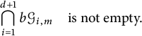$$ \begin{align*}\bigcap_{i=1}^{d+1} b{\mathcal G}_{i, m} \quad \textrm{is not empty.} \end{align*} $$

Indeed, it suffices to show that

(7.1) $$ \begin{align} \bigcap_{i=1}^{d+1} b{\mathcal G}_{i, 0} \quad \textrm{is not empty,} \end{align} $$

since

$$ \begin{align*}\bigcap_{i=1}^{d+1} b{\mathcal G}_{i, 0} \subset \bigcap_{i=1}^{d+1} b{\mathcal G}_{i, m} \end{align*} $$

for all $m \ge 0$ . While for a proof of (7.1), it suffices to note that the set

$$ \begin{align*}\left\{x \in \mathbb{R}^d: x_1=A, x_2=(\delta_3)_2, \dots, x_d=(\delta_{d+1})_d \right\} \subset \bigcap_{i=1}^{d+1} b{\mathcal G}_{i, 0}. \end{align*} $$

To complete the proof, it suffices to follow Conde Alonso’s argument. Namely, we pick a point $a \in \bigcap \limits _{i=1}^{d+1} b{\mathcal G}_{i, 0}$ and we take a small cube centered at a. It is clear that the only way to cover this ball by using the cubes from $\bigcup \limits _{i=1}^{d+1} {\mathcal G}_i$ is to use a cube whose sidelength is at least n. Shrinking the sidelength of the cube as small as we want, this gives a contradiction to the second property in Definition 1.3.

Therefore, this easy lemma suggests the following definition.

Definition 7.4 Given $\delta _1, \dots , \delta _\ell \in \mathbb {R}^d$ , where $\ell \ge 1, \ell \in \mathbb {Z}$ , we say that they are separated if

$$ \begin{align*}(\delta_i)_k \neq (\delta_j)_k \quad (\textrm{mod} \ 1), \end{align*} $$

for all $k \in \{1, \dots , d\}$ and $1 \le i \neq j \le \ell $ .

Now, we are ready to introduce the so-called small-scale lattices.

Definition 7.5 Let $m \ge 0$ and $\delta _1, \dots , \delta _d \in \mathbb {R}^d$ be separated. Then the small-scale lattice associated to $\delta _1, \dots , \delta _d$ at level m is defined as

$$ \begin{align*}{\mathfrak L}(\delta_1, \dots, \delta_d; m):=\bigcap_{i=1}^d b\left[{\mathcal G}(\delta_i)_m\right], \end{align*} $$

where ${\mathcal G}(\delta )_m$ is defined as in Definition 3.1 and $b\left [{\mathcal G}(\delta )_m\right ]$ refers to the union of all the boundary of the cubes in ${\mathcal G}(\delta )_m$ .

Example 7.6 Let us give an example of such a structure (see Figure 4), in which we consider the set ${\mathcal L}\left ( \left (\frac {1}{3}, \frac {1}{3}\right ), \left (\frac {2}{3}, \frac {2}{3}\right ); 1 \right )$ with $d=2$ and $n=2$ . More precisely, in Figure 4, the red dashed lattice represents $b \left [{\mathcal G} \left ( \left (\frac {1}{3}, \frac {1}{3} \right ) \right )_1 \right ]$ , the blue dashed lattice represents $b \left [{\mathcal G} \left ( \left (\frac {2}{3}, \frac {2}{3} \right ) \right )_1 \right ]$ , and the collection of all green points stands for ${\mathcal L}\left ( \left (\frac {1}{3}, \frac {1}{3}\right ), \left (\frac {2}{3}, \frac {2}{3}\right ); 1 \right )$ .

Figure 4:

${\mathcal L}\left ( \left (\frac {1}{3}, \frac {1}{3}\right ), \left (\frac {2}{3}, \frac {2}{3}\right ); 1 \right )$ .

There is an equivalent way to define ${\mathcal L}(\delta _1, \dots , \delta _d; m)$ .

Lemma 7.8 Let $\delta _1, \dots , \delta _d$ be separated. For each $\sigma \in S_d$ , where $S_d$ refers to the finite symmetric group over $\{1, \dots , d\}$ , denote

$$ \begin{align*}\delta_\sigma:=\left( \left(\delta_{\sigma(1)} \right)_1, \dots, \left(\delta_{\sigma(d)} \right)_d \right) \in \mathbb{R}^d. \end{align*} $$

Then, for each $m \ge 0$ , there holds

$$ \begin{align*}{\mathcal L}(\delta_1, \dots, \delta_d; m)=\bigcup_{\sigma \in S_d} {\mathcal A}(\delta_\sigma)_m. \end{align*} $$

Let us denote

$$ \begin{align*}{\mathfrak L}(\delta_1, \dots, \delta_d):=\bigcup_{m \ge 0} {\mathfrak L}(\delta_1, \dots, \delta_d; m) \end{align*} $$

be the union of all small-scale lattices.

We are ready to generalize the concept of far number in dimension-one case.

Definition 7.9 Given $\delta _1, \dots , \delta _d \in \mathbb {R}^d$ being separated, we say $\delta \in \mathbb {R}^d$ is an n-far vector with respect to ${\mathfrak L}(\delta _1, \dots , \delta _d)$ , if there exists some $C>0$ , such that for every $m \ge 0$ , there holds

(7.2) $$ \begin{align} \textrm{dist} \left(b\left[{\mathcal G}(\delta)_m\right], {\mathfrak L}(\delta_1, \dots, \delta_d; m) \right) \ge \frac{C}{n^m}. \end{align} $$

Remark 7.10 While the above definition looks quite different from Definition 1.3 of [Reference Anderson, Hu, Jiang, Olson and Wei2], we can actually motivate our definition from [Reference Anderson, Hu, Jiang, Olson and Wei2]. In the one-dimensional case, the set $\{\delta _1, \dots , \delta _d\}$ reduces to the set $\{0\}$ . Therefore, n-far in the one-dimensional case reduced to checking that

(7.3) $$ \begin{align} \left|\delta-\frac{k}{n^m} \right| \ge \frac{C}{n^m}, \end{align} $$

for $k \in \mathbb {Z}$ and $m \ge 0$ (see Remark 1.4(2) in [Reference Anderson, Hu, Jiang, Olson and Wei2]). Due to such a simple structure, Theorem 2.8 in [Reference Anderson, Hu, Jiang, Olson and Wei2] asserted that $\delta \in \mathbb {R}$ is n-far if and only if the maximal length of tie, that is, the maximal length of consecutive $0$ ’s or consecutive ( $n-1$ )’s in the base n-representation of $\delta $ , is finite.

The key point to generalize the concept of n-far number in higher dimension is to realize that $\delta $ and $\frac {k}{n^m}$ are indeed playing different roles in condition (7.3). More precisely, rewrite (7.3) as

$$ \begin{align*}\left| \left(\delta-\frac{k_1}{n^m} \right)-\frac{k_2}{n^m} \right| \ge \frac{C}{n^m} \end{align*} $$

for $k_1, k_2 \in \mathbb {Z}$ and $m \ge 0$ . Here are the key observations: let $m \ge 0$ be fixed, then:

1. (1) when $k_1$ varies, the set

   $$ \begin{align*}\left\{ \delta-\frac{k_1}{n^m}: k_1 \in \mathbb{Z} \right\} \end{align*} $$
   represents the all the boundary points $b\left [{\mathcal G}(\delta )_m \right ]$ ;

2. (2) when $k_2$ varies, the set

   $$ \begin{align*}\left\{\frac{k_2}{n^m}: k_2 \in \mathbb{Z} \right\} \end{align*} $$
   represents the small-scale lattice ${\mathcal L}(0; m)$ . This is clear from Lemma 7.8.

Hence, an equivalent way to state (7.3) is the following: for any $m \ge 0$ ,

$$ \begin{align*}\textrm{dist} \left( b\left[ {\mathcal G}(\delta)_m \right], {\mathcal L}(0; m) \right) \ge \frac{C}{n^m}, \end{align*} $$

which is precisely (7.2). The key here is that the boundary points and the small-scale lattice align in dimension 1.

Example 7.11 We now illustrate via an example why the idea of generalizing the concept of far numbers to pairwise distances is not sufficient to show that $d+1$ grids are adjacent. Take $\delta _1 = (0,0), \delta _2 = \left (0,\frac {1}{3}, \right )$ and $\delta _3 = \left (\frac {1}{3},\frac {1}{3} \right )$ . Consider the natural pairwise generalization of far where $\delta $ and $\delta '$ are far if $(\delta )_i$ is far from $(\delta ')_i$ for some i. Using this definition, we see that each of these points is far from each other, but $\delta _1, \delta _2, \delta _3$ do no form an adjacent n-adic system. In fact, if one looks at $\mathcal {L}(\delta _1, \delta _2;0)$ , one does not get a lattice, but a set of vertical lines (see Figure 5).

Figure 5:

A nonexample of small-scale lattice: $b[{\mathcal G}(\delta _1)]_0$ (black part), $b[{\mathcal G}(\delta _2)]_0$ (blue part), $b[{\mathcal G}(\delta _3)]_0$ (red part), and the nonexample $b\left [{\mathcal G}(\delta _1)\right ]_0 \cap b\left [{\mathcal G}(\delta _2)\right ]_0$ (green part).

Therefore, this pairwise comparison between points is not enough to determine an adjacent n-adic system and the lattice structure is needed.

7.3 Large-scale sampling, large-scale lattice, and modulated corner sets

The purpose of the last part of section is to introduce all the basic structures with respect to d separated vectors and d location functions, which is used to study the large-scale case. Informally, these structures are the counterparts of the small-scale lattice (see Definition 7.5) and the usual corner sets (see Definition 7.1); however, one new phenomenon for the large scale is that one needs to use the cube $[0, n^j)^d$ to quantify the behavior of the location function (see Theorem 8.1(ii)), and this suggests that we need a localized version of those structures in the large-scale case.

The setting is as follows. Let $\delta _1, \dots , \delta _d \in \mathbb {R}^d$ be separated, ${\vec {\textbf {a}}}_1, \dots , {\vec {\textbf {a}}}_d$ be the d many infinite matrices defined in (3.1), and ${\mathcal L}_{{\vec {\textbf {a}}}_1}, \dots , {\mathcal L}_{{\vec {\textbf {a}}}_d}$ be the corresponding location functions.

Definition 7.12 For each $j>0$ , the large-scale sampling associated to the tuples

$$ \begin{align*}\left(\delta_1, {\vec{\textbf{a}}}_1\right), \dots, \left(\delta_d, {\vec{\textbf{a}}}_d\right) \end{align*} $$

at level j is defined by

$$ \begin{align*}{\mathcal S}_{{\vec{\textbf{a}}}_1, \dots, {\vec{\textbf{a}}}_d}^{\delta_1, \dots, \delta_d}(j):=\left( \bigcap_{k=1}^d b\left[ {\mathcal G}(\delta_k, {\mathcal L}_{{\vec{\textbf{a}}}_k})_{-j}\right]\right) \cap [0, n^j)^d. \end{align*} $$

Example 7.13 Let $d=2, n=2$ , $\delta _1 = \left (\frac {1}{3}, \frac {1}{3} \right )$ , and $\delta _2 = \left (\frac {2}{3}, \frac {2}{3} \right )$ . We illustrate below the large-scale sampling (see Figure 6) for $j=1$ for $\left (\delta _1, {\vec {\textbf {a}}}_1 \right )$ and $\left (\delta _2, {\vec {\textbf {a}}}_2 \right )$ (in the cube $[0,2)^2)$ ) in Figure 6, where

$$ \begin{align*}{\vec{\textbf{a}}}_1:= \begin{pmatrix} 1 & 0 & 1 & 0 & \dots\\ 1 & 0 & 1 & 0 & \dots \end{pmatrix} \end{align*} $$

and

$$ \begin{align*}{\vec{\textbf{a}}}_2:=\begin{pmatrix} 0 & 1 & 0 & 1 & \dots\\ 0 & 1 & 0 & 1 & \dots \end{pmatrix} \end{align*} $$

Figure 6:

An example of large-scale sampling: $A=\delta _1+{\mathcal L}_{ {\vec {\textbf {a}}}_1}(1)=\left (\frac {4}{3}, \frac {4}{3} \right )$ , $B=\delta _2+{\mathcal L}_{{\vec {\textbf {a}}}_2}(1)=\left (\frac {2}{3}, \frac {2}{3} \right )$ , $b\left [{\mathcal G}(\delta _1, {\vec {\textbf {a}}}_1) \right ]_{-1}$ (red part), $b\left [{\mathcal G}(\delta _2, {\vec {\textbf {a}}}_2) \right ]_{-1}$ (blue part), and the large-scale sampling ${\mathcal S}_{{\vec {\textbf {a}}}_1, {\vec {\textbf {a}}}_2}^{\delta _1, \delta _2}(1)$ (green part).

Let us extend the definition of small-scale lattice to the large scales, which can be viewed as a “global” version of the large-scale sampling.

Definition 7.14 For each $m<0$ , the large-scale lattice associated to the tuples

$$ \begin{align*}\left(\delta_1, {\vec{\textbf{a}}}_1\right), \dots, \left(\delta_d, {\vec{\textbf{a}}}_d\right) \end{align*} $$

at level m is defined by

$$ \begin{align*}{\mathcal L}_{{\vec{\textbf{a}}}_1, \dots, {\vec{\textbf{a}}}_d}^{\delta_1, \dots, \delta_d}(m):=\bigcap_{k=1}^d b\left[ {\mathcal G}(\delta_k, {\mathcal L}_{{\vec{\textbf{a}}}_k})_m\right]. \end{align*} $$

We need one more definition to state our main result in large scale.

Definition 7.17 Let $j \ge 0$ , $\delta \in \mathbb {R}^d$ , ${\vec {\textbf {a}}}$ be an infinite matrix defined in (3.1), and ${\mathcal L}_{{\vec {\textbf {a}}}}$ be the associated location function. Then the jth modulated corner set associated to $(\delta , {\vec {\textbf {a}}})$ is defined to be

$$ \begin{align*}(m{\mathcal C})_{{\vec{\textbf{a}}}}^{\delta}(j):=\left( b \left[{\mathcal G}(\delta, {\mathcal L}_{\vec{\textbf{a}}}) \right]_{-j}\right) \cap [0, n^j)^d. \end{align*} $$

Example 7.18 We give an easy example of such a structure (see Figure 7). Here, we take our favorite example, that is, we consider the case when $d=2$ , $n=2, j=1$ , $\delta =\left (\frac {1}{3}, \frac {1}{3} \right )$ , and ${\vec {\textbf {a}}}:= \begin {pmatrix} 1 & 0 & 1 & 0 & \dots \\ 1 & 0 & 1 & 0 & \dots \end {pmatrix}$ .

Figure 7:

$(m{\mathcal C})_{{\vec {\textbf {a}}}}^{\left (\frac {1}{3}, \frac {1}{3} \right )}(1)$ .

In our later application, the modulated corner sets will only be applied to study the ancestors of the zeroth generation, whereas the corner sets defined early will take care of all the generations. More precisely, the modulated corners are important to take care of points near the boundary of the cube $[0, n^j)^d$ that might be close to a corner lying just outside $[0,n^j)^d$ but far from the modulated corner. This remark will be made clearer in the next section and indeed underlies our use of modulated corners.

8.1 Motivation and the structure theorem of adjacency

As mentioned in the introduction, the intuition behind the next theorem originates back to the one-dimensional result (see Theorem 2.2). The main idea to generalize the first condition is already contained in Remark 7.10. More precisely, we can rewrite condition (1) as: there exists some absolute constant $C>0$ , such that for any $k_1, k_2 \in \mathbb {Z}$ and $m \ge 0$ , it holds that

$$ \begin{align*}\left| \left( \delta_1-\frac{k_1}{n^m} \right)-\left( \delta_2-\frac{k_2}{n^m} \right) \right| \ge \frac{C}{n^m}. \end{align*} $$

For simplicity, we may assume both $\delta _1, \delta _2 \in [0, 1)$ , that is, both of them are of unit size (although we do not require such a restriction in our main result). As in Remark 7.10, there are two different ways to interpret the sets

$$ \begin{align*}\left\{\delta_i-\frac{k}{n^m}: k_i \in \mathbb{Z} \right\}, \quad i=1, 2. \end{align*} $$

The first way is to interpret each set as the set of all the boundary points $b\left [ {\mathcal G}(\delta _i)_m\right ]$ , whereas the second way is to treat it as the small-scale lattice ${\mathfrak L}(\delta _i; m)$ . Therefore, we can restate the first condition as

$$ \begin{align*} \delta_1\ \mathit{is}\ n-\mathit{far}\ \mathit{with}\ \mathit{respect}\ \mathit{to}\ {\mathfrak L}(\delta_2)\ \mathit{and}\ \delta_2\ \mathit{is}\ n-far\ \mathit{with}\ \mathit{respect}\ \mathit{to}\ {\mathfrak L}(\delta_1). \end{align*} $$

While for condition (2), note that it is equivalent to the following:

(8.1) $$ \begin{align} 0<\liminf_{j \to \infty} \left| \frac{\delta_1+{\mathcal L}_{{\vec{\textbf{a}}}_1}(j)-\delta_2-{\mathcal L}_{{\vec{\textbf{a}}}_2}(j)}{n^j} \right| \le \limsup_{j \to \infty} \left| \frac{\delta_1+{\mathcal L}_{{\vec{\textbf{a}}}_1}(j)-\delta_2-{\mathcal L}_{{\vec{\textbf{a}}}_2}(j)}{n^j} \right|<1. \end{align} $$

Similarly, there are two ways to interpret the sets (which contain only one element in the one-dimensional case):

(8.2) $$ \begin{align} \left\{ \delta_i+{\mathcal L}_{{\vec{\textbf{a}}}_i}(j) \right\}, \quad i=1, 2, \end{align} $$

for any $j \ge 1$ . The first way is to regard each as a jth modulated corner set, namely, $(m{\mathcal C})_{{\vec {\textbf {a}}}_i}^{\delta _i}(j)$ , whereas the second way is to consider it as a large-scale sampling at level j, that is, ${\mathcal S}_{{\vec {\textbf {a}}}_i}^{\delta _i}(j)$ . If one sets the interpretation of the first set as the modulated corner and of the second set as the large-scale sampling, then additionally there are also two different ways to understand the term

(8.3) $$ \begin{align} \left| \delta_1+{\mathcal L}_{{\vec{\textbf{a}}}_1}(j)-\delta_2-{\mathcal L}_{{\vec{\textbf{a}}}_2}(j) \right|. \end{align} $$

The first way is to treat it as

$$ \begin{align*}\textrm{dist} \left( (m{\mathcal C})_{{\vec{\textbf{a}}}_i}^{\delta_i}(j), {\mathcal S}_{{\vec{\textbf{a}}}_{i'}}^{\delta_{i'}}(j) \right), \end{align*} $$

where $\{i, i'\}=\{1, 2\}$ , whereas the second way is to regard it as the “maximum distance” between these two sets, that is,

$$ \begin{align*}\max_{y' \in {\mathcal S}_{{\vec{\textbf{a}}}_{i'}}^{\delta_{i'}}(j)} \textrm{dev} \left( (m{\mathcal C})_{{\vec{\textbf{a}}}_i}^{\delta_i}(j), y' \right). \end{align*} $$

Note that all these complicated structures (that is, the modulated corner set and large-scale sampling) collapse into a single point in the one-dimensional case, and all those quantities coincide with each other and take the value (8.3); however, in higher dimension, we need to treat them differently.

Here is the main result for the second part, which can be thought as some structure theorem of adjacency with respect to a collection of $d+1\ n$ -adic grids.

Theorem 8.1 The collection of n-adic grids ${\mathcal G}(\delta _1, {\mathcal L}_{{\vec {\textbf {a}}}_1}), \dots , {\mathcal G}(\delta _{d+1}, {\mathcal L}_{{\vec {\textbf {a}}}_{d+1}})$ are adjacent if and only if:

1. (i) For each $i \in \{1, \dots , d+1\}$ , $\delta _i $ is n-far with respect to ${\mathfrak L}\left (\delta _1, \dots , \widehat {\delta _i}, \dots , \delta _{d+1}\right )$ . Here, $\widehat {\delta _i}$ means that in the sequence $\{\delta _1, \dots , \delta _{d+1}\}$ , we remove the term $\delta _i$ .

2. (ii) For each $i \in \{1, \dots , d+1\}$ , there holds

   (8.4) $$ \begin{align} 0&<\liminf_{j \to \infty} \frac{\textrm{dist} \left( (m{\mathcal C})_{{\vec{\textbf{a}}}_i}^{\delta_i} (j), {\mathcal S}_{{\vec{\textbf{a}}}_1, \dots, \widehat{{\vec{\textbf{a}}}_i}, \dots, {\vec{\textbf{a}}}_{d+1}}^{\delta_1, \dots, \widehat{\delta_i}, \dots, \delta_{d+1}}(j) \right)}{n^j} \nonumber \\ & \le \limsup_{j \to \infty} \frac{\max_{y' \in {\mathcal S}_{{\vec{\textbf{a}}}_1, \dots, \widehat{{\vec{\textbf{a}}}_i}, \dots, {\vec{\textbf{a}}}_{d+1}}^{\delta_1, \dots, \widehat{\delta_i}, \dots, \delta_{d+1}}(j)} \textrm{dev}\left( (m{\mathcal C})_{{\vec{\textbf{a}}}_i}^{\delta_i} (j), y' \right)}{n^j} <1. \end{align} $$

Note that in the above statement, for each $j>0$ and $i \in \{1. \dots , d+1\}$ ,

$$ \begin{align*}{\mathcal S}_{{\vec{\textbf{a}}}_1, \dots, \widehat{{\vec{\textbf{a}}}_i}, \dots, {\vec{\textbf{a}}}_{d+1}}^{\delta_1, \dots, \widehat{\delta_i}, \dots, \delta_{d+1}}(j) \end{align*} $$

is a finite set, and hence the maximum value in the limit superior can be attained.

Remark 8.2 Note that the above result is independent of the choice of the representation of the n-grid and hence contains the uniformness result Theorem 2.4 as a particular case. The reason is that the structures that we are working with, that is, the collection of all the boundary points at certain generations, the small-scale lattices, the modulated corner sets, and the large-scale sampling, are independent of the choice of the representations, whereas for the term

$$ \begin{align*}\delta+{\mathcal L}_{{\vec{\textbf{a}}}}(j) \end{align*} $$

(see (8.2) and (8.1)) that we used in our one-dimensional result indeed depends on the particular choices of the representation; more precisely, it is possible for us to find two equivalent presentations ${\mathcal G}(\delta , {\mathcal L}_{{\vec {\textbf {a}}}})$ and ${\mathcal G}(\delta ', {\mathcal L}_{{\vec {\textbf {a}}}'})$ such that

$$ \begin{align*}\delta+{\mathcal L}_{{\vec{\textbf{a}}}}(j)<n^j \le \delta'+{\mathcal L}_{{\vec{\textbf{a}}}'}(j) \end{align*} $$

for j sufficiently large. In such a situation, Theorem 8.1 suggests us to work with the point $\delta '+{\mathcal L}_{{\vec {\textbf {a}}}'}(j)-n^j$ instead of $\delta '+{\mathcal L}_{{\vec {\textbf {a}}}'}(j)$ , and this will guarantee that there is only one limit infimum and one limit superior in (8.4), instead many of them.

8.2 Example revisited

Let us use Theorem 8.1 to verify the adjacency of the dyadic grids considered in Section 5. We start by verifying Condition (i) in Theorem 8.1. This means we have to show:

1. (a) $\delta _1$ is $2$ -far with respect to ${\mathfrak L}\left (\delta _2, \delta _3\right )$ ;

2. (b) $\delta _2$ is $2$ -far with respect to ${\mathfrak L}\left (\delta _1, \delta _3\right )$ ;

3. (c) $\delta _3$ is $2$ -far with respect to ${\mathfrak L}\left (\delta _1, \delta _2\right )$ .

We will show (c). First, it is easy to see that $\{\delta _1, \delta _2, \delta _3\}$ are separated. Note that calculating the quantity (7.2) for $m=1$ reduces to calculating in a “local region” (see the cyan part in Figure 8), as both $b[{\mathcal G}(\delta _3)]_1$ and ${\mathfrak L}(\delta _1, \delta _2; 1)$ behave periodically. Therefore, we can see that

$$ \begin{align*}\textrm{dist} \left(b\left[{\mathcal G}(\delta_3)\right]_1, {\mathfrak L}(\delta_1,\delta_2; 1) \right) = \min\left\{\frac{1}{3}-\frac{1}{5}, \ \frac{1}{5}-\frac{1}{6} \right\} = \frac{1/15}{2}. \end{align*} $$

Figure 8:

$b[{\mathcal G}(\delta _3)]_1$ (red part), the small-scale lattice ${\mathfrak L}(\delta _1, \delta _2; 1)$ (green part), the line segment with length $\frac {1}{3}-\frac {1}{5}=\frac {2}{15}$ (the horizontal magenta colored line), and the line segment with length $\frac {1}{5}-\frac {1}{6}=\frac {1}{30}$ (the vertical magenta colored line).

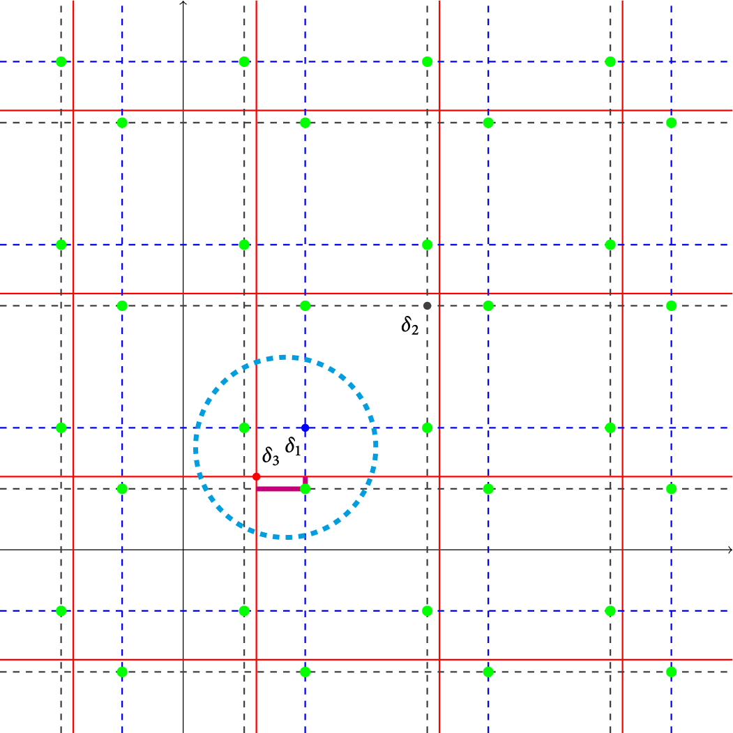
It turns out that this case $m=1$ already illustrates the main point. The case $m=0$ is even easier, and for all other $m>0$ , we will get either

$$ \begin{align*} \textrm{dist} \left(b\left[{\mathcal G}(\delta_3)\right]_m, {\mathfrak L}(\delta_1,\delta_2; m) \right) &= \inf_{k_1, k_2 \in \mathbb{Z}} \left|\left(\frac{1}{3} \pm \frac{k_1}{2^m} \right)- \left(\frac{1}{5} \pm \frac{k_2}{2^m} \right) \right| \\ &\geq \inf_{k_1, k_2 \in \mathbb{Z}} \left|\frac{2}{15} - \frac{k}{2^m} \right| \ge \frac{C}{2^m} \end{align*} $$

by techniques in [Reference Anderson, Hu, Jiang, Olson and Wei2, Proposition 2.4] (see also Lemma 3 in [Reference Anderson1]), or a similar claim where $\frac {1}{3}$ is replaced by $\frac {2}{3}$ . The other calculations for (a) and (b) are similar. For example, by an easy modification of the above arguments, we have, for any $m \ge 0$ ,

$$ \begin{align*}\textrm{dist} \left(b\left[{\mathcal G}(\delta_1)\right]_m, {\mathfrak L}(\delta_2,\delta_3; m) \right) \end{align*} $$

(this is for (a)) is either

$$ \begin{align*}\inf_{k_1, k_2 \in \mathbb{Z}} \left|\left(\frac{2}{3} \pm \frac{k_1}{2^m} \right)- \left(\frac{1}{3} \pm \frac{k_2}{2^m} \right) \right| \end{align*} $$

or

$$ \begin{align*}\inf_{k_1, k_2 \in \mathbb{Z}} \left|\left(\frac{1}{5} \pm \frac{k_1}{2^m} \right)- \left(\frac{1}{3} \pm \frac{k_2}{2^m} \right) \right|, \end{align*} $$

which is clearly bounded below by some $\frac {C}{2^m}$ , where C is independent of the choice of m. We leave the details to the interested reader.

We now verify Condition (ii). We first calculate the limit infimum, and begin by examining the case $j=1$ . In this case, it is clear from Figure 9 that

$$\begin{align*}\frac{\textrm{dist} \left( (m{\mathcal C})_{{\vec{\textbf{a}}}_1}^{\delta_1} (1), {\mathcal S}_{{\vec{\textbf{a}}}_2, {\vec{\textbf{a}}}_{3}}^{\delta_2, \delta_{3}}(1) \right)}{2} = \frac{1}{3}, \end{align*}$$

whereas

$$\begin{align*}\frac{\textrm{dist} \left( (m{\mathcal C})_{{\vec{\textbf{a}}}_2}^{\delta_2} (1), {\mathcal S}_{{\vec{\textbf{a}}}_1, {\vec{\textbf{a}}}_{3}}^{\delta_1, \delta_{3}}(1) \right)}{2} = \frac{\textrm{dist} \left( (m{\mathcal C})_{{\vec{\textbf{a}}}_3}^{\delta_3} (1), {\mathcal S}_{{\vec{\textbf{a}}}_1, {\vec{\textbf{a}}}_{2}}^{\delta_1, \delta_{2}}(1) \right)}{2} = \frac{|2/3-1/5|}{2} =\frac{7}{15}. \end{align*}$$

Figure 9:

All modulated corner sets $(m{\mathcal C})_{{\vec {\textbf {a}}}_i}^{\delta _i}(1)$ for $i=1, 2, 3$ (red parts) and all corresponding large-scale samplings ${\mathcal S}_{{\vec {\textbf {a}}}_1, \dots , \widehat {{\vec {\textbf {a}}}_i}, \dots , {\vec {\textbf {a}}}_3}^{\delta _1, \dots , \widehat {\delta _i}, \dots , \delta _3}(1)$ for $i=1, 2, 3$ (green parts).

Let us also calculate the case when $j=2$ (see Figure 10). In this case, we have

$$\begin{align*}\frac{\textrm{dist} \left( (m{\mathcal C})_{{\vec{\textbf{a}}}_2}^{\delta_2} (2), {\mathcal S}_{{\vec{\textbf{a}}}_1, {\vec{\textbf{a}}}_{3}}^{\delta_2, \delta_{3}}(2) \right)}{4} = \frac{1}{3}, \end{align*}$$

whereas

$$\begin{align*}\frac{\textrm{dist} \left( (m{\mathcal C})_{{\vec{\textbf{a}}}_1}^{\delta_1} (2), {\mathcal S}_{{\vec{\textbf{a}}}_2, {\vec{\textbf{a}}}_{3}}^{\delta_2, \delta_{3}}(2) \right)}{4} = \frac{\textrm{dist} \left( (m{\mathcal C})_{{\vec{\textbf{a}}}_3}^{\delta_3} (2), {\mathcal S}_{{\vec{\textbf{a}}}_1, {\vec{\textbf{a}}}_{2}}^{\delta_1, \delta_{2}}(2) \right)}{4} = \frac{4/3-1/5}{2} =\frac{17}{60}. \end{align*}$$

Figure 10:

All modulated corner sets $(m{\mathcal C})_{{\vec {\textbf {a}}}_i}^{\delta _i}(2)$ for $i=1, 2, 3$ (red parts) and all corresponding large-scale samplings ${\mathcal S}_{{\vec {\textbf {a}}}_1, \dots , \widehat {{\vec {\textbf {a}}}_i}, \dots , {\vec {\textbf {a}}}_3}^{\delta _1, \dots , \widehat {\delta _i}, \dots , \delta _3}(2)$ for $i=1, 2, 3$ (green parts).

Similarly, the cases $j=1, 2$ (that is, $m=-1$ and $-2$ , respectively) contain all the main ideas for the large-scale case (that is, $m<0$ ). Recall that, for $j \ge 0$ ,

$$ \begin{align*}\delta_1+{\mathcal L}_{{\vec{\textbf{a}}}_1}(j)= \begin{cases} \left(\frac{2^{j}}{3}, \frac{2^{j}}{3} \right), & \hfill j \ \textrm{even}, \\ \\ \left(\frac{2^{j+1}}{3}, \frac{2^{j+1}}{3} \right), & \hfill j \ \textrm{odd}, \end{cases} \quad \delta_2+{\mathcal L}_{{\vec{\textbf{a}}}_2}(j)= \begin{cases} \left(\frac{2^{j+1}}{3}, \frac{2^{j+1}}{3} \right), & \hfill j \ \textrm{even}, \\ \\ \left(\frac{2^{j}}{3}, \frac{2^{j}}{3} \right), & \hfill j \ \textrm{odd}, \end{cases} \end{align*} $$

and

$$ \begin{align*}\delta_3+{\mathcal L}_{{\vec{\textbf{a}}}_3}(j) \equiv \left(\frac{1}{5}, \frac{1}{5} \right). \end{align*} $$

This suggests that the first two limit infimums, which are

$$ \begin{align*}\liminf_{j \to \infty} \frac{\textrm{dist} \left( (m{\mathcal C})_{{\vec{\textbf{a}}}_1}^{\delta_1} (j), {\mathcal S}_{{\vec{\textbf{a}}}_2, {\vec{\textbf{a}}}_{3}}^{\delta_2, \delta_{3}}(j) \right)}{2^j} \quad \textrm{and} \quad \liminf_{j \to \infty} \frac{\textrm{dist} \left( (m{\mathcal C})_{{\vec{\textbf{a}}}_2}^{\delta_2} (j), {\mathcal S}_{{\vec{\textbf{a}}}_1, {\vec{\textbf{a}}}_{3}}^{\delta_1, \delta_{3}}(j) \right)}{2^j}, \end{align*} $$

are either

$$ \begin{align*}\lim_{j \to \infty} \frac{2^{j+1}/3-2^j/3}{2^j}=\frac{1}{3} \end{align*} $$

or

$$ \begin{align*}\lim_{j \to \infty} \frac{2^j/3-1/5}{2^j}=\frac{1}{3}. \end{align*} $$

To see this, one may consider two different cases by requiring j being even or being odd, the desired claim will then follow from plotting the corresponding modulated corner sets and large-scale samplings out, as the first two graphs illustrated in Figure 9.

While for the third limit infimum, that is,

$$ \begin{align*}\liminf_{j \to \infty} \frac{\textrm{dist} \left( (m{\mathcal C})_{{\vec{\textbf{a}}}_3}^{\delta_3} (j), {\mathcal S}_{{\vec{\textbf{a}}}_1, {\vec{\textbf{a}}}_{2}}^{\delta_1, \delta_{2}}(j) \right)}{2^j}, \end{align*} $$

we can see that it will be

$$ \begin{align*}\lim_{j \to \infty} \frac{2^j/3-1/5}{2^j}=\frac{1}{3}. \end{align*} $$

One may consult the third graph in Figure 9 for a visualization of this case. Overall, we can take $\frac {1}{3}$ as the limit infimum in Condition (ii) of our main result.

The calculations for the limit supreme are similar and can be visualized from Figure 9. More precisely, we can see that the quantity

$$ \begin{align*}\max_{i=1,2,3} \left[\limsup_{j \to \infty} \frac{\max_{y' \in {\mathcal S}_{{\vec{\textbf{a}}}_1, \dots, \widehat{{\vec{\textbf{a}}}_i}, \dots, {\vec{\textbf{a}}}_3}^{\delta_1, \dots, \widehat{\delta_i}, \dots, \delta_3}(j)} \textrm{dev}\left( (m{\mathcal C})_{{\vec{\textbf{a}}}_i}^{\delta_i} (j), y' \right)}{2^j}\right] \end{align*} $$

is the limit

$$ \begin{align*}\lim_{j \to \infty} \frac{2^{j+1}/3 - 1/5}{2^j} = \frac{2}{3}. \end{align*} $$

This verifies Condition (ii) in Theorem 8.1.▪