


1. Introduction to wave focussing
Focussing of moderate amplitude, progressive surface waves can often in turn produce unexpectedly large waves. At oceanic scales, spatial wave focussing, where large amplitude waves form persistently in specific regions (Chavarria, Le Gal & Le Bars Reference Chavarria, Le Gal and Le Bars2018; Torres et al. Reference Torres, Lloyd, Dolan and Weinfurtner2022), can produce waves powerful enough to damage or capsize ships. A famous example is the Aghulas current region (The Editors of Encyclopaedia Britannica 2024) known for giant waves and shipping accidents (Mallory Reference Mallory1974; Smith Reference Smith1976). The role of current generated refractive focussing leading to the birth of such giant waves, specifically in the Agulhas, was anticipated by Peregrine (Reference Peregrine1976) (also see figure 8 in Dysthe, Krogstad & Müller (Reference Dysthe, Krogstad and Müller2008) and § 2 in White & Fornberg (Reference White and Fornberg1998)). Refractive focussing of surface waves (Peregrine Reference Peregrine1986) has also been exploited to design ‘lenses’, i.e. submerged structures in a water basin which focus incoming divergent, circular waves (see figure 1a in Stamnes et al. (Reference Stamnes, Løvhaugen, Spjelkavik, Mei, Lo and Yue1983)), these being motivated from wave generation of power (McIver Reference McIver1985; Murashige & Kinoshita Reference Murashige and Kinoshita1992).
In addition to spatial focussing, spatiotemporal focussing also occurs (Dysthe et al. Reference Dysthe, Krogstad and Müller2008), where large wave amplitudes manifest at specific locations in space, albeit briefly. Spatiotemporal focussing has obvious relevance not only towards understanding, for example, rogue (freak) waves in the ocean (Charlie Wood 2020), but also to our current study (next section). The physical mechanisms underlying spatiotemporal focussing have been distinguished further into linear and nonlinear dispersive focussing (§§ 4.2 and 4.3, Dysthe et al. (Reference Dysthe, Krogstad and Müller2008)). Linear dispersive focussing of progressive waves relies on constructive interference exploiting the dispersive nature of surface gravity waves and is particularly simple to understand in the deep-water limit. For unidirectional wave packets in deep water, generated from a wavemaker oscillating harmonically at frequency  $\varOmega$ at one end of a sufficiently long wave flume, the energy propagation velocity (group velocity) of the packet is $c_g = {g}/{2\varOmega }$ where $g$ is acceleration due to gravity. If the wavemaker frequency varies linearly from $\varOmega _1$ to $\varOmega _2$ ( $\varOmega _1 > \varOmega _2$) following ${{\rm d}\varOmega }/{{\rm d}t} = -({g}/{2x_f})$ within the time interval $[t_1, t_2]$, Longuet-Higgins (Reference Longuet-Higgins1974) showed that the energy of each wave packet emitted during this period will converge at $x = x_f$ simultaneously at $t = t_f$ (see Brown & Jensen Reference Brown and Jensen2001). This focussing of wave energy thus causes a momentary but significant increase in energy density at $x_f$ manifested as a transient, large amplitude wave at that location around time $t_f$. This technique has been discussed in Davis & Zarnick (Reference Davis and Zarnick1964) and its variants have been employed extensively to generate breaking waves in the laboratory in a predictable manner in two (Rapp & Melville Reference Rapp and Melville1990) and three dimensions (Johannessen & Swan Reference Johannessen and Swan2001; Wu & Nepf Reference Wu and Nepf2002; McAllister et al. Reference McAllister, Draycott, Davey, Yang, Adcock, Liao and van den Bremer2022) as well as in other related contexts such as generation of a parasitic capillary on large amplitude waves (Xu & Perlin Reference Xu and Perlin2023).
On the other hand, in nonlinear dispersive focussing, the modulational instability (Benjamin & Feir Reference Benjamin and Feir1967) of a uniform, finite-amplitude wavetrain (Stokes wave) plays a crucial role. This instability can cause the wavetrain to split into groups, where focussing within a group can produce a wave significantly larger than the others (Zakharov, Dyachenko & Prokofiev Reference Zakharov, Dyachenko and Prokofiev2006). For further details on nonlinear focussing, we refer readers to the review by Onorato et al. (Reference Onorato, Residori, Bortolozzo, Montina and Arecchi2013).
1.1. Spatiotemporal focussing at gravito–capillary scales
Following this brief introduction to large-scale focussing, we now shift our attention to length scales where gravitational and capillary restoring forces are nearly equivalent. Our study aims to achieve an analytical understanding of wave focussing at these shorter scales. Below, we illustrate two examples where such small-scale focussing can be readily observed.
Stuhlman (Reference Stuhlman1932) investigated the formation of drops from collapsing bubbles with diameters under  $0.12$ cm in water–air interfaces and $0.15$ cm in benzene–air interfaces. He hypothesised that these drops emerged from Worthington jets created by the collapse of the bubble cavity. However, contemporary research identifies this as just one of two mechanisms responsible for drop generation (Villermaux, Wang & Deike Reference Villermaux, Wang and Deike2022). The first high-speed ( ${\approx }6000$ frames per second) images of jet formation were reported by MacIntyre (Reference MacIntyre1968, Reference MacIntyre1972) (see original experiments by Kientzler et al. (Reference Kientzler, Arons, Blanchard and Woodcock1954)). Interestingly, these studies demonstrated that the surface ripples are created by the retraction of the circular rim of the relaxing bubble cavity. These ripples travel towards the cavity base before the jet emerges. In the words of MacIntyre (Reference MacIntyre1972) (see abstract) ‘ $\ldots$ an irrotational solitary capillary ripple precedes the main toroidal rim transporting mass along the surface at approximately $90\,\%$ of its phase velocity. The convergence of this flow creates opposed jets
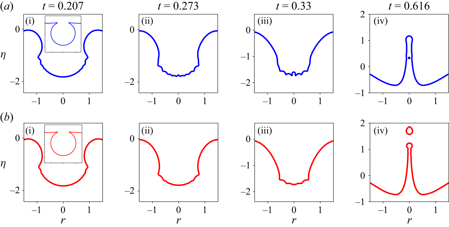
  $\ldots$’. The seminal work by Duchemin et al. (Reference Duchemin, Popinet, Josserand and Zaleski2002) of collapsing bubbles (much smaller than their capillary length scale) at a gas–liquid interface was able to resolve this focussing process, via direct numerical simulations (DNS) of the axisymmetric Navier–Stokes equations without gravity. Figure 1 depicts the generation of an axisymmetric, wavetrain focussing towards the base of the bubble cavity (also the symmetry axis) for two different Ohnesorge numbers $(Oh)$ and at a fixed Bond number $(Bo)$. The Bond number $Bo\equiv {\rho ^Lg\hat {R}_b^2}/{T}$ determines the bubble shape, and the Ohnesorge number $Oh\equiv {\mu ^L}/{\sqrt {\rho ^LT\hat {R}_b}}$ accounts for the ratio of viscous to capillary forces. Here $\rho ^L,\mu ^L,T, \hat {R}_b$ are the lower fluid density, lower fluid viscosity, coefficient of surface tension and equivalent radius of the bubble, respectively. We refer the readers to Deike (Reference Deike2022), Sanjay (Reference Sanjay2022) and Gordillo & Blanco-Rodríguez (Reference Gordillo and Blanco-Rodríguez2023) for recent advances on the study of bubble collapse and jet formation mechanisms.
An example of capillary wave focussing obtained from DNS conducted using the open-source code Basilisk (Popinet & Collaborators Reference Popinet2013–2024). The initial cavity shape, inset in (a i,b i), is obtained by solving the Young–Laplace equation with gravity to determine the shape of a static bubble at the free surface (without its cap). In centimetre–gram–second (CGS) units, initial bubble radius  $0.075$, surface tension $T=72$, gravity $g=-981$, density $\rho ^{L}=1.0$ and $\rho ^{U}=0.001$ for upper and lower fluid. Panel (a) (blue) simulations are conducted using zero viscosity for both gas (above) and liquid (below). Panel (b) (red) simulations have dynamic viscosity $\mu ^{U}=0.0001$ and $\mu ^{L}=0.01$. Axes are non-dimensionalised using initial bubble radius. Time is non-dimensionalised using the capillary time scale $t = {\hat {t}}/{\sqrt {{\rho \hat {R}_b^3}/{T}}}$. For panel (a) $Bo \equiv {\rho ^{L} g\hat {R}_b^2}/{T}=0.076$ and $Oh={\mu ^{L}}/{\sqrt {\rho ^{L} T \hat {R}_b}} = 0$; for panel (b) $Bo=0.076$ and $Oh=0.0043$.
Another example of axisymmetric focussing of surface waves was highlighted in the study by Longuet-Higgins (Reference Longuet-Higgins1990), where several interesting observations were noted. Longuet-Higgins (Reference Longuet-Higgins1990) studied the inverted conical shaped ‘impact cavities’ seen in experiments and simulations (Oguz & Prosperetti Reference Oguz and Prosperetti1990) of a liquid droplet falling on a liquid pool. The author compared these cavities with an exact solution to the potential flow equations without surface tension or gravity (Longuet-Higgins Reference Longuet-Higgins1983), where the free surface (gas–liquid interface) took the form of a cone at all times. The apex of this cone (i.e. the impact cavity) is often seen to contain a bulge (see figure 2a in Longuet-Higgins (Reference Longuet-Higgins1990)) and the formation of this was attributed to (we quote, § 6 first paragraph in Longuet-Higgins (Reference Longuet-Higgins1990)) ‘a ripple on the surface of the cone converging towards the axis of symmetry’, thus highlighting the role of wave focussing once again. Longuet-Higgins (Reference Longuet-Higgins1990) insightfully remarked that this convergence process would be similar to the radially inward propagation of a circular ripple on a water surface. The interface shape could thus be approximated as being due to the linear superposition of an initial, localised wave packet (generated by distorting an initially flat surface) whose Fourier–Bessel representation  $F(k)$ ( $k$ being the wavenumber) slowly varies on a time scale $\bar {t}$ (i.e. slow compared with the wave packet propagation time scale $t$). Longuet-Higgins (Reference Longuet-Higgins1990) thus posits that the shape of the perturbed interface $\eta (r,t, \bar {t})$ may be represented as
 \begin{equation} \eta(r,t,\bar{t}) = \int_{\Delta k} F(k,\bar{t}){\mathrm{J}}_{0}(kr)\exp\left(I\sigma(k) t\right)k \,{\rm d}k, \end{equation}
where  ${\mathrm {J}}_{0}$ is the Bessel function, $r$ is the radial coordinate and the spectrum of the surface perturbation $F(k,\bar {t})$ evolves slowly on a time scale $\bar {t}$, $I\equiv \sqrt {-1}$ and $\sigma (k)$ satisfies the dispersion relation for capillary waves (see equation (6.2) in Longuet-Higgins (Reference Longuet-Higgins1990)). Note that if the slow variation of $F(k,\bar {t})$ over $\bar {t}$ is supressed, (1.1) represents the solution to the linearised Cauchy–Poisson problem with an initial surface distortion whose Hankel transform is $F(k)$. Longuet-Higgins (Reference Longuet-Higgins1990), however, did not report any systematic comparison of available experimental or simulation data (Oguz & Prosperetti Reference Oguz and Prosperetti1990) with (1.1) although the author anticipated that nonlinearity could become important during the convergence (see the last paragraph on page 405 of Longuet-Higgins (Reference Longuet-Higgins1990)).
Our current study is partly motivated by the aforementioned observations of Longuet-Higgins (Reference Longuet-Higgins1990) and Duchemin et al. (Reference Duchemin, Popinet, Josserand and Zaleski2002) and aims at obtaining an analytical description of spatiotemporal wave focussing at these short scales. We seek an initial, localised surface distortion which produces a wavetrain, and whose radial convergence may be studied analytically, at least in the potential flow limit. We refer the reader to the review by Eggers, Sprittles & Snoeijer (Reference Eggers, Sprittles and Snoeijer2024) where this limit corresponding to Ohnesorge  $Oh=0$ is discussed. In the next section we present a localised initial surface distortion which is expressible as a linear superposition of Bessel functions (Fourier–Bessel series). It will be seen that this distortion generates a surface wavetrain which focuses towards the symmetry axis of the container. We emphasise that the wavetrains or the solitary ripple seen in Kientzler et al. (Reference Kientzler, Arons, Blanchard and Woodcock1954) and Longuet-Higgins (Reference Longuet-Higgins1990), respectively, have different physical origins compared with the ones we study here. However, following Longuet-Higgins (Reference Longuet-Higgins1990) we intuitively expect there are aspects of their convergence which do not sensitively depend on how these are generated in the first place.
Of particular relevance to us is also the interesting study by Fillette, Fauve & Falcon (Reference Fillette, Fauve and Falcon2022) who investigated forced capillary–gravity waves in a cylindrical container. These waves were generated via a vertically vibrating ring at the gas–liquid interface. The authors showed that the steady shape of the interface is well represented by the third-order, (nonlinear) time-periodic solution due to Mack (Reference Mack1962). The agreement between the analytical model and experimental data is particularly good around  $r=0$, although differences persist away from the symmetry axis (see their figure 4b). With increasing forcing amplitude, the authors note an interesting transition from the linear to the nonlinear regime followed by a jet ejection regime. We demonstrate in Appendix D that a similar transition is also seen for our initial condition (see discussion in the next paragraph) albeit our study excludes external forcing. Due to the absence of forcing, it becomes feasible to carry out a first principles mathematical analysis of the wave-focussing regime, as has been reported here.
While wavetrain convergence and jet formation may often be concomitant, as apparent from the bubble collapse simulations in figure 1, the two phenomena are distinct. Figure 3 of Deike et al. (Reference Deike, Ghabache, Liger-Belair, Das, Zaleski, Popinet and Séon2018), for example, describes experimental investigations of an air bubble bursting at a silicon oil–air interface producing a jet, but without any visible signature of a converging wavetrain towards the collapsing bubble base. On the other hand, the converging wavetrain in the shape oscillations generated due to two coalescing bubbles (Zhang & Thoroddsen (Reference Zhang and Thoroddsen2008); their figure 12), lead to rapid interfacial oscillations at the focal point, but no signature of pinch-off or a liquid jet. When a converging wavetrain and a liquid jet are both present, the dynamics of the latter can be affected by the former quite non-trivially. The fastest jet in such cases can occur at an ‘optimal’ value of liquid viscosity, rather than in the inviscid limit; see experiments and figure 3(b) of Ghabache et al. (Reference Ghabache, Antkowiak, Josserand and Séon2014a) in the context of bubble bursting. In view of this rather complex aforementioned behaviour, it becomes desirable to have first principles studies of cavity collapse with and without an accompanying wavetrain. The spatially localised interface deformation considered in this study (figure 3), permits access to these phenomena independently, through a tuning parameter. As shown in Appendix D, for small cavity depth (relative to its width), the initial distortion generates a train of radially inward focussed waves (after reflection), which we label as ‘wave focussing’ and whose physics is of interest here. At larger cavity depth, a jet emerges already at short time due to ‘flow focussing’. Notably, this jet is formed significantly before wall reflections can generate a radially inward propagating wavetrain. The study in Basak, Farsoiya & Dasgupta (Reference Basak, Farsoiya and Dasgupta2021) investigated such a jet, albeit obtained from a single Bessel function. In contrast, we study here the wave focussing regime where no such jet is generated.
As further motivation of our current study, we note that the bubble whose collapse is described in figure 1, is nearly spherical initially as its Bond number is low ( ${\ll }1$). The highly deformed, multivalued initial shape of such a bubble (inset of figure 1a i) precludes expressing it as a Fourier–Bessel series. In contrast, figure 2(a) depicts the bubble shape in the converse limit of large Bond number. Here the bubble shape appears like a cavity albeit with sharp protrusions. Such an initial shape (with some smoothing of the protrusions) is amenable to expression in a Fourier–Bessel series, whose coefficients may be evaluated in time. The cavity treated in this study, may thus be considered a crude approximation to a bubble at high Bond number. For numerical reasons, we have chosen our initial deformation to be a cavity with smooth humps (see figure 3) in contrast to the bubble shape with kinks in figure 2(a). We emphasise that for such an initial deformation as studied here, the physical origin of the focussing wave train that appears in our simulations is different from that of Gordillo & Rodríguez-Rodríguez (Reference Gordillo and Rodríguez-Rodríguez2019). Consequently, the focussing of the wavetrain is not the same as that of the wavetrain in classical bursting of bubbles at low $Bo$. However, qualitative similarities in certain aspects may be expected between the two situations and are studied here (see Appendix E).
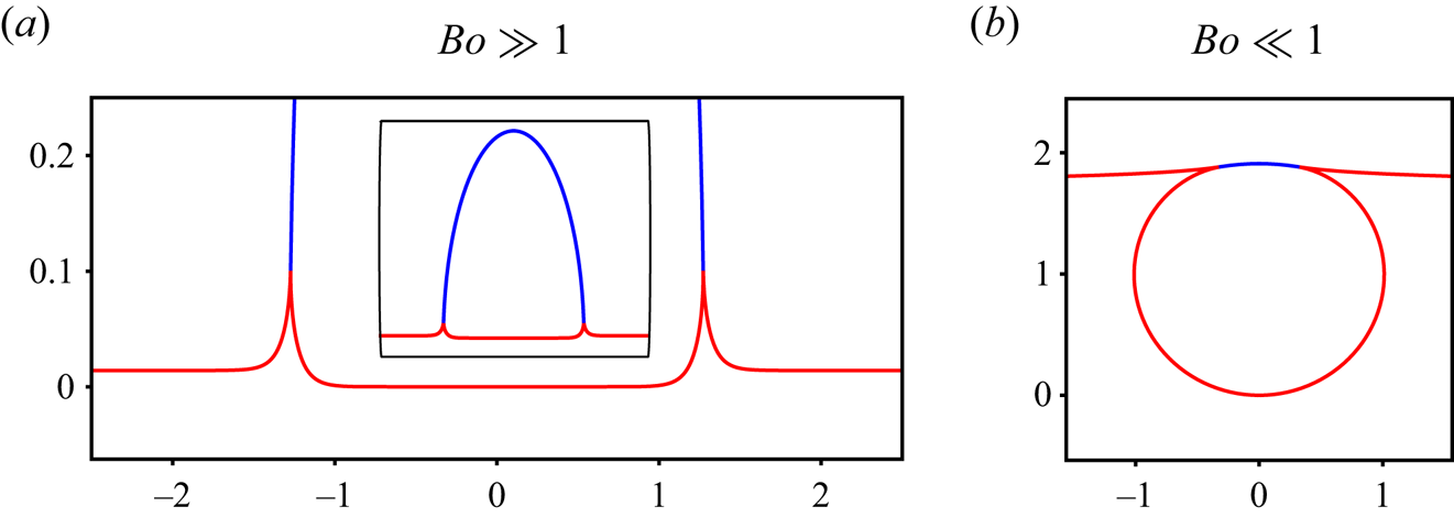
The effect of change of Bond number on the shape of a static bubble. (a) The bubble shape for  $Bo =222\gg 1$. (b) An air bubble corresponding to $Bo =0.076\ll 1$, also see inset in figure 1(a). As the Bond number is increased, an increasingly larger fraction of the bubble shifts upwards (compared with the mean interface level at large distance) and its ‘rim’, see sharp corners in (b), distorts into vertically pointing kinks seen in (a). For $Bo\gg 1$, the bubble shape is a single-valued function $\eta (r)$, the red curve in (a), and provides the motivation for the initial interface distortion (albeit significantly smoother) in figure 3 and treated analytically in this study. The curves in blue in (a,b) represent the bubble cap. The inset in (a), depicts the entire bubble including its cap while the main figure, highlights the bubble ‘rim’.
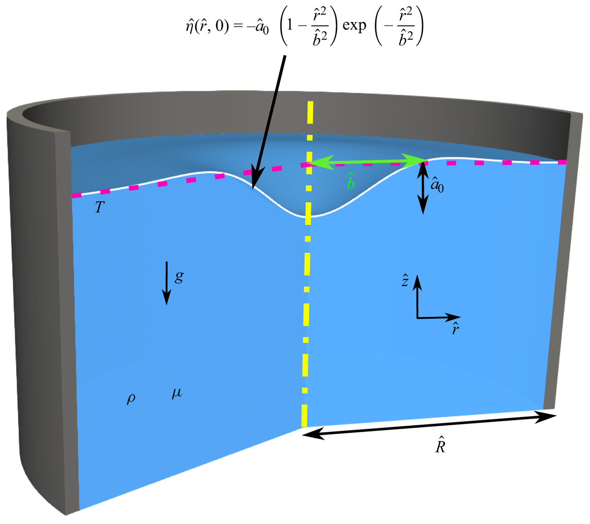
A (not to scale) cross-sectional representation of the initial interface distortion  $\hat {\eta }(\hat {r},0)$ shaped as a cavity of half-width $\hat {b}$ and depth $\hat {a}_0$ in a cylinder of radius $\hat {R}$ filled with liquid (in blue). The functional form chosen for $\hat {\eta }(\hat {r},0)$ was first proposed by Miles (Reference Miles1968) and represents a volume preserving distortion on radially unbounded domain. The red dotted line indicates the unperturbed level of the free surface of the liquid pool. The gas–liquid surface tension is $T$. Liquid density and viscosity are $\rho$ and $\mu$, respectively, $g$ is gravity. The cavity shape can be considered as a crude representation to the $Bo\gg 1$ bubble shape in figure 2 with the kinks smoothened drastically. It must be emphasised that our initial condition and the resulting wavetrain are significantly different from that of a bursting bubble. However, we intuitively expect that there may be qualitative similarities between the two processes and that it is possible to learn something about one by studying the other, which incidentally has the advantage of analytical tractability.
We develop an inviscid nonlinear theory for the focussing of a concentric wavetrain resulting from the aforementioned a priori imposed free-surface deformation. This theory developed from first principles here has no fitting parameters and helps delineate those aspects of focussing which may be accounted for by linear theory compared with nonlinear features. In a series of earlier theoretical and computational studies from our group (Farsoiya, Mayya & Dasgupta Reference Farsoiya, Mayya and Dasgupta2017; Basak et al. Reference Basak, Farsoiya and Dasgupta2021; Kayal, Basak & Dasgupta Reference Kayal, Basak and Dasgupta2022; Kayal & Dasgupta Reference Kayal and Dasgupta2023), we have solved the initial-value problem corresponding to delocalised, initial interface distortions in the form of a single Bessel function  $({\mathrm {J}}_{0}(kr))$ at gravity-dominated large scales (Kayal & Dasgupta Reference Kayal and Dasgupta2023), gravito–capillary intermediate scales (Farsoiya et al. Reference Farsoiya, Mayya and Dasgupta2017; Basak et al. Reference Basak, Farsoiya and Dasgupta2021) and capillarity-dominated small scales (Kayal et al. Reference Kayal, Basak and Dasgupta2022) (also see the recent study in Dhote et al. (Reference Dhote, Kumar, Kayal, Goswami and Dasgupta2024) for a delocalised initial perturbation on a sessile bubble). In contrast to these studies where the initial perturbation was spatially delocalised, we study here a spatially localised initial excitation. Apart from the obvious advantage of easier experimental realisation of this (see Ghabache, Séon & Antkowiak (Reference Ghabache, Séon and Antkowiak2014b) for experiments at gravity dominated scales), this initial condition has the additional advantage that already at linear order, a radially propagating concentric wavetrain is obtained and one can ask how does this converge at the axis of symmetry? In contrast, for the single Bessel function initial excitation as in Basak et al. (Reference Basak, Farsoiya and Dasgupta2021), Kayal et al. (Reference Kayal, Basak and Dasgupta2022) and Kayal & Dasgupta (Reference Kayal and Dasgupta2023), at linear order one obtains only a standing wave and it is necessary to proceed to quadratic order and beyond to generate the focussing wavetrain.
The manuscript is structured as follows. Section 2 illustrates the time evolution of a relaxing cavity and introduces the analytical equations for wave evolution. Section 3 compares these analytical results with DNS. Finally, the paper culminates with discussions and outlook in § 4.
2. Time evolution of a relaxing cavity
As shown in figure 3, the system consists of a cylindrical container of radius  $\hat {R}$ filled with quiescent liquid (indicated in blue). As we do not model the upper fluid in our theory, here onwards the superscript $L$ is dropped from the variables representing fluid properties. For simplicity of analytical calculation, the cylinder is assumed to be infinitely deep and the gas–liquid density ratio is kept fixed at $0.001$ for DNS only. In our theoretical calculations, we approximate the gas–liquid interface as a free surface and neglect any motion in the gas phase (although, it is modelled in our DNS). Some of the relevant length scales are the gravito–capillary length $l_c \equiv \sqrt {T/\rho g} \approx 2.7\,{\rm mm}$ and the viscocapillary length scale $l_\mu \equiv \mu ^2/\rho T \approx 0.01\,\mathrm {\mu }{\rm m}$. For our chosen half-width of the initial interface perturbation ( $\hat {b}=8.0\,{\rm mm}$), these length scales justify the inclusion of both capillarity as well as gravity in the theoretical calculation while neglecting viscosity at the leading order. However, we stress that viscosity is known to have a non-monotonic effect on wave focussing in a collapsing bubble, as demonstrated by Ghabache et al. (Reference Ghabache, Antkowiak, Josserand and Séon2014a). Their figure 3 shows that the jet velocity during bubble bursting varies non-monotonically with increasing viscosity. Thus, the fastest jets occur not in an inviscid system but at an ‘optimal’ viscosity. In what follows, we employ potential flow equations in our theory and do not treat the boundary layers expected to be generated at the air–water interface and the cylinder walls (Mei & Liu Reference Mei and Liu1973). We will address the inclusion of viscous effects later in the study.
Before delving into the theoretical formulation, it is instructive to discuss the phenomenology of the problem. Figure 4(a–i) depict the interface at various time instants as obtained from DNS. These are obtained by solving the inviscid, axisymmetric and incompressible Euler's equations with surface tension and gravity in cylindrical coordinates (Basilisk, Popinet & Collaborators Reference Popinet2013–2024) (a script file is available as Supplementary material (Kayal Reference Kayal2024)). The images in figure 4 are obtained by generating the surface of revolution of axisymmetric DNS data. As shown in figure 4(a), the interface is initially distorted in the shape of an axisymmetric, stationary and localised perturbation. As this cavity relaxes, waves are generated which travel outward reflecting off the wall (between figure 4e and figure 4f). This produces a wavetrain which focusses at the symmetry axis of the container ( $r=0$). One notes the formation of a small dimple-like structure at the symmetry axis in figure 4(h). In § 3, we will demonstrate that neither the dimple nor other interface features around the symmetry axis can be explained by the linear theory.
Wave focussing observed in DNS from the cavity-shaped interface distortion at  $t=0$ a). The figure is to be read from left to right and top to bottom for the progression of time. After the waves reflect off the cylinder wall (between panels (e) and (f); the confining walls are not shown), they focus inwards towards $r=0$ producing strongly nonlinear oscillations of increasing amplitude. The arrows indicate the instantaneous direction of wave motion. The DNS parameters may be read from Case $1$ in table 1.

2.1. Governing equations: potential flow
We now turn to the theoretical analysis of the phenomenology illustrated in figure 4. In the base state, we consider a quiescent pool of liquid with density  $\rho$ and surface tension $T$ contained in a cylinder of radius $\hat {R}$. For analytical simplicity, we assume this pool is infinitely deep compared with the wavelength of the excited interface waves. For further simplicity, we assume that the solid–liquid contact angle at the cylinder wall is always fixed at ${\rm \pi} /2$ and the contact line is free to move ( $\partial _nv_t = 0$). This is the simplest contact line condition which allows for reflection of waves at the boundary without complicating the analytical treatment of the problem (Snoeijer & Andreotti Reference Snoeijer and Andreotti2013). The variables $\hat {\eta }(\hat {r},\hat {t})$ are used to represent the axisymmetric perturbed interface (see figure 1) and $\hat {\phi }(\hat {r},\hat {z},\hat {t})$ is the disturbance velocity potential; $\hat {r}$ and $\hat {z}$ being the radial and axial coordinates in cylindrical geometry, respectively. Variables with the dimensions of length (e.g. $\hat {r},\hat {z},\hat \eta$) and time ( $\hat {t}$) are scaled using length and time scales $L \equiv \hat {R}$ and $T_0 \equiv \sqrt {{\hat {R}}/{g}}$, respectively. The velocity potential $\hat {\phi }$ is non-dimensionalised using the scale $L^2/T_0$. Under the potential flow approximation, the non-dimensional governing equations and boundary conditions governing perturbed quantities are
 \begin{gather} \frac{\partial^2\phi}{\partial r^2}+\frac{1}{r}\frac{\partial\phi}{\partial r}+\frac{\partial^2\phi}{\partial z^2} = 0, \end{gather}
 \begin{gather}\frac{\partial\eta}{\partial t}+\left(\frac{\partial\eta}{\partial r}\right)\left(\frac{\partial\phi}{\partial r}\right)_{z=\eta} - \left(\frac{\partial\phi}{\partial z}\right)_{z=\eta} = 0, \end{gather}
 \begin{gather}\left(\frac{\partial\phi}{\partial
t}\right)_{z=\eta}+\eta+\frac{1}{2}\left\{\left(\frac{\partial\phi}{\partial
r}\right)^2+\left(\frac{\partial\phi}{\partial
z}\right)^2\right\}_{z=\eta}\nonumber\\ \quad -
\frac{1}{Bo}\left\{\frac{\dfrac{\partial^2\eta}{\partial
r^2}}{\left\{ 1+\left(\dfrac{\partial\eta}{\partial
r}\right)^2\right\}^{{3}/{2}}}+\frac{1}{r}\frac{\dfrac{\partial\eta}{\partial
r}}{\left\{1+\left(\dfrac{\partial\eta}{\partial
r}\right)^2\right\}^{{1}/{2}}}\right\} =0,
\end{gather}
\begin{gather}\left(\frac{\partial\phi}{\partial
t}\right)_{z=\eta}+\eta+\frac{1}{2}\left\{\left(\frac{\partial\phi}{\partial
r}\right)^2+\left(\frac{\partial\phi}{\partial
z}\right)^2\right\}_{z=\eta}\nonumber\\ \quad -
\frac{1}{Bo}\left\{\frac{\dfrac{\partial^2\eta}{\partial
r^2}}{\left\{ 1+\left(\dfrac{\partial\eta}{\partial
r}\right)^2\right\}^{{3}/{2}}}+\frac{1}{r}\frac{\dfrac{\partial\eta}{\partial
r}}{\left\{1+\left(\dfrac{\partial\eta}{\partial
r}\right)^2\right\}^{{1}/{2}}}\right\} =0,
\end{gather} \begin{gather}\int_{0}^{1}r\eta(r,t)\,{\rm d}r=0,\quad \left(\frac{\partial\phi}{\partial r}\right)_{r=1}= 0, \end{gather}
 \begin{gather}\lim_{z\to-\infty}\phi \to \text{finite} \end{gather}
 \begin{gather}\eta(r,t=0) ={-}\varepsilon\left(1 - \frac{r^2}{b^2}\right)\exp\left(-\frac{r^2}{b^2}\right) = \sum_{m=1}^{N}\eta_m(0){\mathrm{J}}_{0}(k_m r),\nonumber\\ \qquad \frac{\partial\phi}{\partial n}(r,z = \eta(r,0),t=0) = 0, \end{gather}
where  $\varepsilon >0$ and $n$ in (2.1h) is a distance coordinate measured normal to the free surface at $t=0$. The dimensionless parameters are defined as follows: ${1}/{Bo} \equiv \alpha \equiv {T}/{\rho g \hat {R}^2}$, representing the inverse Bond number (based on the cylinder radius); $b \equiv {\hat {b}}/{\hat {R}}$ is the dimensionless measure of cavity width; and $\varepsilon \equiv {\hat {a}_0}/{\hat {R}}$ is the dimensionless measure of cavity depth (see figure 3 caption for the meaning of the symbols). Here onwards, we use $\alpha$ to represent the inverse Bond number.
In cylindrical, axisymmetric coordinates (2.1a) is the Laplace equation, (2.1b) and (2.1c) are the kinematic boundary condition and the Bernoulli equation applied at the free surface, respectively. Equation (2.1d) restricts initial interfacial distortions to those which are volume conserving while (2.1e) enforces no-penetration at the cylinder wall. Equation (2.1f) is the finiteness condition at infinite depth.
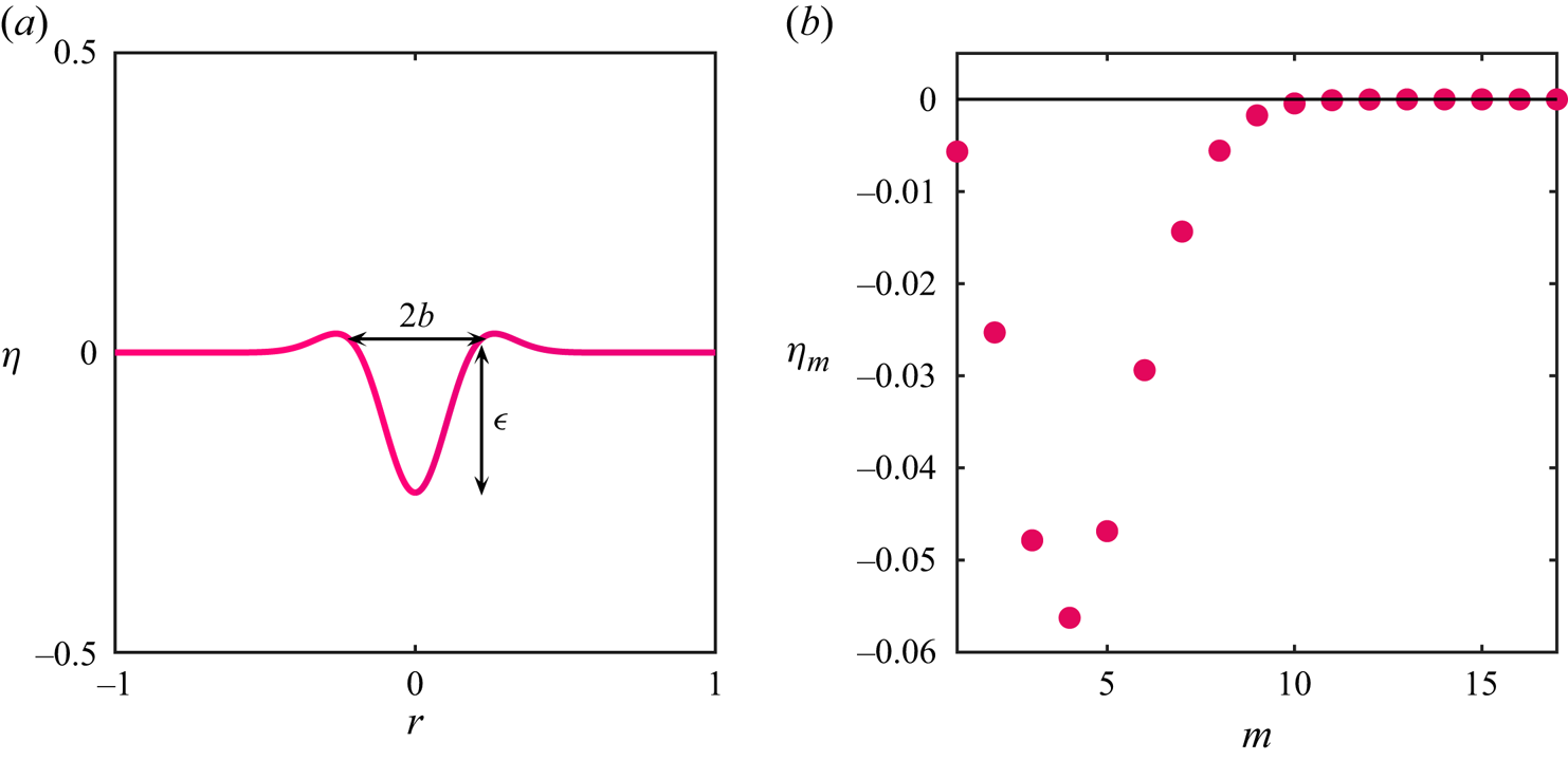
Equation (2.1g,h) represent the initial conditions. We decompose the initial interface distortion, i.e.  $\eta (r,t=0)=-\varepsilon (1 - {r^2}/{b^2})\exp (-({r^2}/{b^2}))$ (Miles Reference Miles1968), into its Fourier–Bessel series as indicated by the second equality sign in (2.1g) and ${\mathrm {J}}_1(k_m)=0$ for $m \in \mathbb {Z}^+$ (from (2.1e); note the identity $\mathrm {J}_0'({\cdot })=-\mathrm {J}_1({\cdot })$, the prime indicating a derivative). The numerical values of the coefficients $\eta _m$ at $t=0$, i.e. $\eta _m(0) \ (m=1,2,3,\ldots )$ in (2.1g) are determined from the orthogonality relation between Bessel functions, i.e. $\eta _m(0)={\int _0^{1}\,{\rm d}r\;r\textrm {J}_0(k_m r)\eta (r,0)}/{\int _0^{1}\,{\rm d}r \;r\textrm {J}_0^2(k_m r)}$. A sample representation of the initial condition and its Fourier–Bessel coefficients is presented in figures 5(a) and 5(b), respectively, where it is seen that approximately $17$ wavenumbers are excited initially. Subject to these initial and boundary conditions presented in (2.1a–h), we need to determine the amplitudes $\eta _m(t),\, m=1,2,3\ldots$ as a function of time and this is carried out next.
(a) The gas–liquid interface initially deformed as a cavity of half-width  $b = {\hat {b}}/{\hat {R}}$ and depth $\varepsilon \equiv {\widehat {a_0}}/{\hat {R}}$ (cavity shape at $t=0$). (b) The coefficients $\eta _m(0)$ are obtained by decomposing the initial distorted interface. For this initial distortion, $\varepsilon =0.091,b=0.187$. It is seen that only the first 10 or so Bessel functions/wavenumbers are excited initially (Bessel function coefficients). For accuracy, we consider the energy in the first seventeen initially ( $m=1,2,3,\ldots,17$).
2.2. Equations for  $\eta _j(t)$

In this section we solve the initial, boundary-value problem posed in (2.1a–h). We derive equations governing the time evolution of the coefficients  $\eta _j(t)$ up to quadratic order (i.e. terms which are cubic or higher in the coefficients are neglected). The approach for doing this is classical and was laid out in Hasselmann (Reference Hasselmann1962) in Cartesian coordinates although their initial conditions were random functions in contrast to the deterministic initial distortion posed in (2.1g). The procedure below closely follows the approach of Nayfeh (Reference Nayfeh1987), who derived similar equations (his equations (14) and (15)) in the context of the Faraday instability (i.e. with vertical oscillatory forcing) including gravity but not surface tension (Nayfeh Reference Nayfeh1987) in his analysis. In contrast to forced waves being studied by Nayfeh (Reference Nayfeh1987), we consider free waves in our current study and include both surface tension and gravity in the analysis. We first expand $\phi$ and $\eta$ in (2.1) as
 \begin{equation} \phi(r,z,t)=\sum_{m=1}^\infty \phi_m(t)\textrm{J}_0(k_mr)\exp(k_mz), \quad\eta(r,t)=\sum_{m=1}^\infty \eta_m(t)\textrm{J}_0(k_mr). \end{equation}
By construction, each term in the expansion in (2.1) satisfies the Laplace equation (2.1a), (2.1d) (the integral mass conservation condition evaluates to be numerically very small for the chosen parameters) and (2.1e) as well as the finiteness condition (2.1f). Taylor expanding (2.1b) and (2.1c) about  $z=0$ we obtain
 \begin{gather} \frac{\partial\eta}{\partial t}-\left(\frac{\partial\phi}{\partial z}\right)_{z=0}-\left(\frac{\partial^2\phi}{\partial z^2}\right)_{z=0}\eta+\frac{\partial\eta}{\partial r}\left(\frac{\partial\phi}{\partial r}\right)_{z=0}+\text{H.O.T}=0, \end{gather}
 \begin{gather}\left(\frac{\partial\phi}{\partial t}\right)_{z=0}+\eta\left(\frac{\partial^2\phi}{\partial t \partial z}\right)_{z=0}+\eta + \frac{1}{2}\left\{\left(\frac{\partial\phi}{\partial r}\right)^2+\left(\frac{\partial\phi}{\partial z}\right)^2\right\}_{z=0}\nonumber\\ -\;\alpha\left\{\frac{\partial^2\eta}{\partial r^2}+\frac{1}{r}\frac{\partial\eta}{\partial r}\right\} + \text{H.O.T}=0 \end{gather}
where  $\text {H.O.T}$ represents higher-order terms. Substituting expansions (2.2a,b) into (2.3a,b) and using orthogonality relations between Bessel functions we obtain for $n,p,m \in \mathbb {Z}^+$ the following:
 \begin{gather} \frac{{\rm d}\eta_n}{{\rm
d}
t}-k_n\phi_n(t)+\sum_{m,p}\big(D_{npm}-k_m^2C_{npm}\big)\phi_m(t)\eta_p(t)=0,
\end{gather}
\begin{gather} \frac{{\rm d}\eta_n}{{\rm
d}
t}-k_n\phi_n(t)+\sum_{m,p}\big(D_{npm}-k_m^2C_{npm}\big)\phi_m(t)\eta_p(t)=0,
\end{gather}
 \begin{gather}\frac{{\rm d}\phi_n}{{\rm
d} t}+\big(1+\alpha k_n^2\big)\eta_n(t)+\sum_{m,p}k_m
C_{npm}\left(\frac{{\rm d}\phi_m}{{\rm d}
t}\right)\eta_p(t)\nonumber\\ \quad +\;\frac{1}{2}\sum_{m,p}\big(D_{npm}+k_mk_pC_{npm}\big)\phi_m(t)\phi_p(t)=0
\nonumber\\ n = 1,2,3 \ldots.
\end{gather}
\begin{gather}\frac{{\rm d}\phi_n}{{\rm
d} t}+\big(1+\alpha k_n^2\big)\eta_n(t)+\sum_{m,p}k_m
C_{npm}\left(\frac{{\rm d}\phi_m}{{\rm d}
t}\right)\eta_p(t)\nonumber\\ \quad +\;\frac{1}{2}\sum_{m,p}\big(D_{npm}+k_mk_pC_{npm}\big)\phi_m(t)\phi_p(t)=0
\nonumber\\ n = 1,2,3 \ldots.
\end{gather}
The nonlinear interaction coefficients  $C_{npm}$ and $D_{npm}$ in (2.4) are related as (Nayfeh Reference Nayfeh1987)
 \begin{equation} D_{npm}=\frac{1}{2}\big(k_p^2+k_m^2-k_n^2\big)C_{npm} \end{equation}
and  $C_{npm}={\int _{0}^1 r\textrm {J}_0(k_nr)\textrm {J}_0(k_pr)\textrm {J}_0(k_mr)\,{\rm d}r}/{\int _{0}^1r\textrm {J}^2_0(k_nr)\,{\rm d}r}$. For the benefit of the reader, the detailed proof of (2.5) is provided in Appendix A. Retaining self-consistently up to quadratic-order terms, (2.4a) and (2.4b) may be combined into a second-order equation for $\eta _n$ alone. This is
 $$\begin{gather} \dfrac{{\rm d}^2\eta_n}{{\rm d} t^2}+\omega_n^2\eta_n+k_n\sum_{m,p}\left[1+\frac{k_p^2-k_m^2-k_n^2}{2k_mk_n}\right]C_{npm}\left(\dfrac{{\rm d}^2\eta_m}{{\rm d} t^2}\right)\eta_p \nonumber\\ +\dfrac{1}{2}k_n\sum_{m,p}\left[1+\dfrac{k_p^2+k_m^2-k_n^2}{2k_mk_p}+\dfrac{k_p^2-k_m^2-k_n^2}{k_mk_n}\right]C_{npm}\left(\dfrac{{\rm d}\eta_m}{{\rm d} t}\right)\left(\frac{{\rm d}\eta_p}{{\rm d} t}\right)=0. \end{gather}$$
Note that  $\omega _n$ is the linear oscillation frequency of the $n$th mode, viz. $\omega _n\equiv \sqrt {k_n(1+\alpha k_n^2)}$ (the effect of the nonlinear terms due to curvature in (2.3b) and thus surface tension, appears only through the linear-order dispersion relation up to second order). We solve the coupled ordinary differential equation (ODE) (2.6) numerically subject to the initial conditions discussed earlier for $n=1,2,3,\ldots 34$ (i.e. twice the initial number, see figure 5b) using ‘DifferentialEquations.jl’, an open-source package by Rackauckas, Nie & Collaborators (Reference Rackauckas and Nie2017) and collaborators. The ‘DifferentialEquations.jl‘ automatically chooses an ODE solver based on stiffness detection algorithms as described by Rackauckas & Nie (Reference Rackauckas and Nie2019). The Julia script file can be found in Kayal (Reference Kayal2024). We note that while numerically solving (2.6), we compute ${{\rm d}^2\eta _m}/{{\rm d} t^2}$ in the third term of the equation (the nonlinear term) via the linear estimate, viz., ${{\rm d}^2\eta _m}/{{\rm d} t^2}=-\omega _m^2 \eta _m$. Interestingly, the solution to (2.6) shows instability albeit only at large time (compared with the focussing time) when high wavenumbers ( $k$) appear in our model. This instability could either be numerical or physical and possibly related to instability of finite-amplitude capillary waves. Further investigations are necessary to ascertain the origin of this and is outside the scope of this study. As the instability occurs outside the time window of our study, it does not impact the results presented in this work. We thus restrict ourselves to numerical solutions to (2.6) within the time period of our interest where this instability does not appear.
As benchmarking of our numerical solution procedure, we first solve (2.6) employing the single Bessel function initial surface distortion that was studied in Basak et al. (Reference Basak, Farsoiya and Dasgupta2021), i.e. in our current notation  $\eta (r,t=0) = \varepsilon {\mathrm {J}}_{0}(l_5\;r),\;\varepsilon > 0$ where $l_5=16.4706$ is the fifth non-trivial root of the Bessel function ${\mathrm {J}}_1$. For this initial condition, the second-order accurate solution is expectedly of the form
 \begin{equation} \eta(r,t)= \varepsilon \eta_1(r,t) + \varepsilon^2 \eta_2(r,t), \end{equation}
where explicit expressions for  $\eta _1$ and $\eta _2$ were provided in Basak et al. (Reference Basak, Farsoiya and Dasgupta2021) (we note the slight difference in non-dimensionalisation of length between the current study and the one by Basak et al. (Reference Basak, Farsoiya and Dasgupta2021) involving a factor of
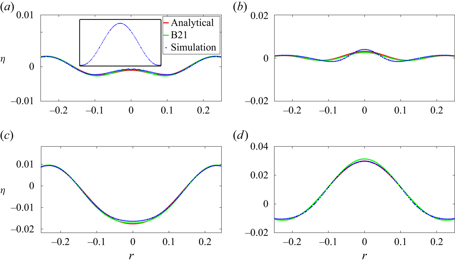
  $l_q$). Figure 6 demonstrates a comparison between the prediction of (2.7) (indicated in the figure as ‘B21’ for Basak et al. (Reference Basak, Farsoiya and Dasgupta2021)), the solution obtained from solving (2.6) with the same initial condition (labelled in the figure as ‘analytical’) and the numerical simulation from Basilisk (depicted as ‘simulation’). Figure 6 demonstrates good agreement between the three, thereby providing confidence on our numerical procedure for solving (2.6).
Benchmarking of our solution procedure for solving the coupled ODEs in (2.6) against inviscid DNS (indicated as ‘simulation’ in the legend of panel (a)) and analytical predictions by Basak et al. (Reference Basak, Farsoiya and Dasgupta2021), indicated as ‘B21’. For DNS, the dimensionless parameters are  $\varepsilon \equiv {a_0}/{\hat {R}} = \tfrac {0.5}{16.4706} = 0.03, \alpha = 0.004$ and $Oh=0$. Note that the initial condition here has a crest around $r=0$, see the inset of panel (a). Here (a) $t = 0.303$; (b) $t= 0.409$; (c) $t = 0.772$; (d) $t=1.029$.
3. Comparison of DNS with theory
3.1. Description
We have used the open-source code Basilisk (Popinet & Collaborators Reference Popinet2013–2024) to solve the Navier–Stokes equation with an interface viz.
 \begin{gather} \boldsymbol{\nabla}\boldsymbol{\cdot}\boldsymbol{u}=0, \end{gather}
 \begin{gather}\frac{\partial\boldsymbol{u}}{\partial t}+\boldsymbol{\nabla}\boldsymbol{\cdot}(\boldsymbol{u\bigotimes u})={-}\frac{\boldsymbol{\nabla}p}{\rho}+g+\frac{T}{\rho}\kappa \delta_s \boldsymbol{n}+\nu\nabla^2\boldsymbol{u}, \end{gather}
 \begin{gather}\frac{\partial f}{\partial t}+\boldsymbol{\nabla}\boldsymbol{\cdot}(f\boldsymbol{u})=0. \end{gather}
Here,  $\boldsymbol {u},p,\kappa$, $T$ and $f$ are the velocity field, pressure field, interface curvature, surface tension and the colour-function field, respectively. Basilisk is a one-fluid solver where the colour function $f$ takes values $0$ and $1$ in the two phases with the interface being represented geometrically using the volume-of-fluid algorithm in cells where $0 < f < 1$. The density and viscosity are represented as a weighted average of the respective values of the two phases, employing the colour function as the weight. Figure 7 depicts the simulation domain, the wall labelled 1 is the symmetry axis, and the liquid and gas are indicated in different colours. We have solved (3.1), (3.2) and (3.3) numerically in cylindrical axisymmetric coordinates, using an adaptive mesh based on temporal changes of the colour function $f$, and velocity $\boldsymbol {u}$. Grid resolution for different cases are provided in table 1. In all the viscous simulations treated in the manuscript, we have used free-slip walls with a $90^{\circ }$ contact angle, in order to be compatible with a freely moving contact line and obviate the well-known contact line singularity (Snoeijer & Andreotti Reference Snoeijer and Andreotti2013). By using free-slip conditions, we maintain consistency with the analytical expressions used in our study and facilitate a more direct comparison between our numerical results and theoretical predictions. This boundary condition naturally enforces a $90^{\circ }$ contact angle at the wall, setting a vanishing gradient for the colour function close to the wall, which is consistent with the assumptions in the theoretical model far from the centre of the cavity. For discussions, we refer to Wildeman et al. (Reference Wildeman, Visser, Sun and Lohse2016) which shows that the free-slip condition with a $90^{\circ }$ contact angle effectively eliminates dissipation close to the contact line, allowing us to focus on the interfacial dynamics that are central to our study.
Simulation domain. Only half of the domain is depicted, due to the axis of symmetry (side labelled  $1$). For both viscous as well as inviscid simulations, the boundaries labelled $2,3$ and $4$ are modelled as free-slip walls.
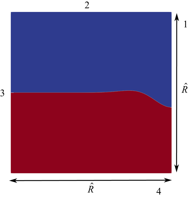
All dimensional lengths are indicated with a hat. Values are quoted in CGS units. In all of the cases we have used  $\hat {R}=4.282$ cm, $\hat {b}=0.8$ cm, $T=72\,{\rm dyne}\,{\rm cm}^{-1}$, $g=-981\,{\rm cm}\,{\rm s}^{-2}$, $\rho =1\,{\rm gm}\,{\rm cm}^{-3}$. These imply dimensionless values $b\equiv {\hat {b}}/{\hat {R}}=0.187$, $\alpha \equiv {T}/{\rho g \hat {R}^2}=0.004$. Here $Oh$ has been defined using $\hat {b}$, in order to be comparable to its value for a bursting bubble where radius of the bubble is considered for defining $Oh$. One may obtain a new Ohnesorge number $Oh^{'}$ based on $\hat {R}$ by using the formulae $Oh' \equiv {\mu }/{\sqrt {\rho T \hat {R}}}=Oh\times b^{1/2}$ with $b\equiv {\hat {b}}/{\hat {R}}$. The maximum grid resolution reported here are in powers of two. The conditions for adaptivity may be found in further detail in the script files (Kayal Reference Kayal2024).

3.2. Comparison
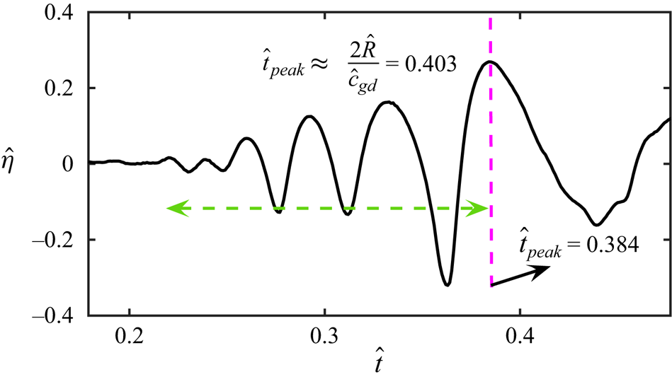
In this section, we compare results from our DNS with the theory discussed in § 2. Before this, it is instructive to rationalise the reflection process and estimate its duration. To do this, we observe that the Fourier–Bessel spectrum of the initial interface distortion prominently features a peak at  $m=4$ (see figure 5b). A rough estimate of the time required for the energy associated with any wavenumber excited in the initial spectrum to complete a return trip (from $\hat {r}=0$ to the wall and back) can be derived from linear theory. When this return time is estimated for the dominant wavenumber in the initial spectrum, we expect the numerical value to roughly coincide with the generation time of the largest amplitude oscillation at $\hat {r}=0$ during the focussing process. This is illustrated in figure 8, where the time signal from tracking the interface at $\hat {r}=0$ is presented (Case 2 in table 1). Note that this figure uses dimensional variables, denoted with hats. After the outward travelling waves move away, the interface at $\hat {r}=0$ remains relatively quiescent, as indicated by the nearly flat time signal around $\hat {t}=0.2$ s. As a result of reflection, the energy associated with every wavenumber $k$ present initially focusses back to $\hat {r}=0$, this return trip is carried out with its group velocity $\hat {c}_{g} = ({g + 3(T/\rho ) k^2})/({2\sqrt {gk + Tk^3/\rho }})$. In figure 5(b), the dominant wavenumber is $k_d = {l_4}/{\hat {R}}$ and the largest oscillation at $\hat {r}=0$ during the focussing process is seen to be generated at $\hat {t}_{peak} = 0.384$ s from figure 8. Using the linear estimate $\hat {t}_{peak} \approx {2\hat {R}}/{\hat {c}_{gd}}$ where $\hat {c}_{gd}$ is the group velocity of the dominant wavenumber, we obtain the value $0.403$ s which is reasonably close to the observed $\hat {t}_{peak}=0.384$ s.
Time signal of the interface at  $\hat {r}=0$. The green line indicates approximately the time window when focussing takes place at $\hat {r}=0$.
In the collage of images in figures 9 and 10, we present the shape of the interface as a function of time for Cases  $1$ and $2$ in table 1, respectively, comparing this with linear and nonlinear theoretical predictions. The only difference between these two figures is in the value of $\varepsilon$, all other dimensionless numbers remaining the same. Here linear theory implies solution to (2.6) without the nonlinear terms. Note that this is equivalent to superposition of the form $\eta (r,t) = \sum _{m=1}^{17}\eta _m(0){\mathrm {J}}_{0}(k_mr)\cos (\omega _m t)$ where $\omega _m(k_m)$ satisfies the gravito–capillary dispersion relation for deep water. In figure 9, the transition from outward propagating waves to inward propagating ones occur between figure 9(c) and figure 9(d). For figure 9(a), figure 9(b) and figure 9(c) it is evident that linear theory represents the outgoing waves accurately. However, as focussing commences from figure 9(d) onwards, we notice significant differences between linear theory and (inviscid) DNS. Interestingly, second-order theory seems to predict the shape of the interface around $r=0$ quite well. Figure 10 shows a more intense scenario than figure 9, featuring a larger $\varepsilon =0.091$. The transition from predominantly linear to nonlinear behaviour occurs between figure 10(c) and figure 10(d), representing outgoing and incoming waves, respectively. Notably, sharp dimple-like structures emerge around $r=0$, as seen in figure 10(h), which are well described by nonlinear theory. Additionally, the tendency to form jets (although no clear jet is visible), as seen in figure 10(j), is noteworthy, although the nonlinear theory is only qualitatively accurate in this context. We refer the reader to the accompanying Supplementary Movie 1 available at https://doi.org/10.1017/jfm.2024.1089 ( $\varepsilon = 0.061$) and Movie 2 ( $\varepsilon = 0.091$), see additional Supplementary material which visualises these.
Waves generated from the cavity shaped interface distortion at  $t=0$ (inset of panel (a)). We compare the interface shape as a function of time as predicted by linear theory (L, solid blue line), second-order nonlinear theory (N, solid green line) and (inviscid) DNS (Sim, red symbols). The waves reflect off the cylinder wall at $r=1$ (not shown) and focus back towards $r=0$ generating oscillations of increasing amplitude. This corresponds to Case $1$ of table 1 with $\varepsilon = 0.061$. To highlight the difference between linear and nonlinear predictions, the figures have been plotted up to $r=0.5$ instead of the entire radial domain up to $r=1$. The arrows depict the instantaneous direction of motion of the waves. Here (a) $t=0.166$; (b) $t=0.439$; (c) $t=1.075$; (d) $t=4.056$; (e) $t=4.117$; (f) $t=4.435$; (g) $t=4.753$; (h) $t=5.358$; (i) $t=5.615$; (j) $t=5.842$.
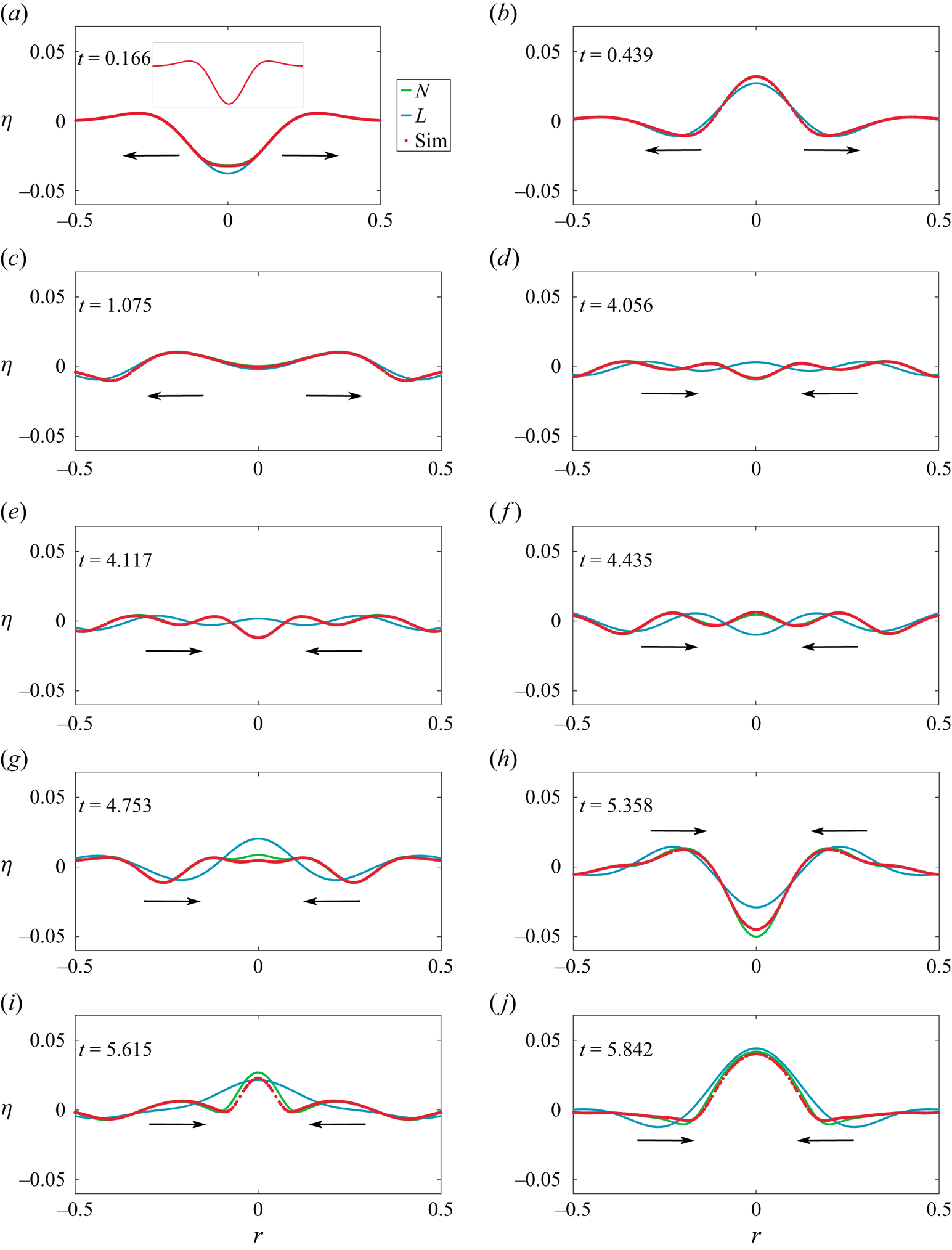
The same as figure 9, but for  $\varepsilon =0.091$ corresponding to Case $2$ in table 1. Note the good qualitative agreement between nonlinear theory and (inviscid) DNS but not linear theory, in capturing the dimple in (h). Also note the large amplitude oscillations at $r=0$ with a tendency to generate narrow jet-like structures (i,j), although no jets are seen. Here (a) $t=0.166$; (b) $t=0.439$; (c) $t=1.075$; (d) $t=4.056$; (e) $t=4.117$; (f) $t=4.435$; (g) $t=4.753$; (h) $t=5.358$; (i) $t=5.165$; (j) $t=5.842$.
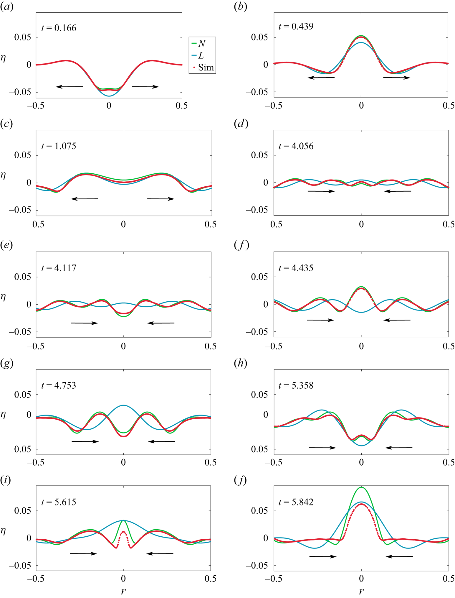
3.3. Role of nonlinearity at $r=0$

Figures 9 and 10 show that although the linear solution is a reasonable model for the interface evolution before reflection, it shows deviation from the fully nonlinear simulation at the axis of symmetry during radial convergence of the wavetrain. Towards understanding this better, we provide two sets of analysis in the following subsections. In § 3.3.1, we analyse the time-periodic solution by Mack (Reference Mack1962), investigating the role of nonlinearity generated bound components around  $r=0$. In § 3.3.2, we analyse the initial deformation as a Bessel function, akin to Basak et al. (Reference Basak, Farsoiya and Dasgupta2021). It will be seen from both analysis that bound components play an important role in the interface deformation around $r=0$.
3.3.1. Comparison with time-periodic solution
Unlike the initial interface distortion studied so far which leads to aperiodic behaviour, there also exist finite-amplitude deformations which generate time-periodic oscillations. Such finite-amplitude, time-periodic solutions are the standing-wave counterparts of the well-known Stokes travelling wave. In rectangular coordinates, such a standing-wave solution was first developed by Rayleigh (Strutt Reference Strutt1915) and in further detail by Penney et al. (Reference Penney, Price, Martin, Moyce, Penney, Price and Thornhill1952). This was extended to radially bounded, cylindrical geometry for finite liquid depth in Mack (Reference Mack1962). In the deep-water limit, Mack's solution contains three parameters, all appearing in the ‘free wave’ (see below) part of the solution represented by  $\tilde {a}_0 {\rm J}_0(k_q {\hat {r}}/{\hat {R}}),\, q=1,2,3,\ldots$. These in turn lead to two non-dimensional parameters viz. $\tilde {\epsilon } \equiv {\tilde {a}_0}/{\hat {R}}$ and a positive integer $q=1,2,3,\ldots$ specifying the number of zero crossings of ${\rm J}_0$ within the radial domain, a measure of crest-to-crest distance of the perturbation ( ${\rm J}_0$ is not periodic but becomes so asymptotically). In non-dimensional form the time-periodic solution of Mack (Reference Mack1962) may be written as
 \begin{align}
\eta(r,\tilde{t};\tilde{\epsilon},q) &=
T_0(r;\tilde{\epsilon},q) +
T_1(r;\tilde{\epsilon},q)\cos(2{\rm \pi}\tilde{t}) +
T_2(r;\tilde{\epsilon},q)\cos(4{\rm \pi}\tilde{t})\nonumber\\ &\quad +
T_3(r;\tilde{\epsilon},q)\cos(6{\rm \pi}\tilde{t}),
\end{align}
\begin{align}
\eta(r,\tilde{t};\tilde{\epsilon},q) &=
T_0(r;\tilde{\epsilon},q) +
T_1(r;\tilde{\epsilon},q)\cos(2{\rm \pi}\tilde{t}) +
T_2(r;\tilde{\epsilon},q)\cos(4{\rm \pi}\tilde{t})\nonumber\\ &\quad +
T_3(r;\tilde{\epsilon},q)\cos(6{\rm \pi}\tilde{t}),
\end{align}
where  $\tilde {t}\equiv {\omega \hat {t}}/{2{\rm \pi} }$. Mack (Reference Mack1962) obtained expressions for $T_0(r), T_1(r)$ and $T_2(r)$ for $q=1$ employing $\tilde {\epsilon }$ as perturbative parameter (up to $O(\tilde {\epsilon }^3)$) and expressions for these along with the nonlinear frequency $\omega (\tilde {\epsilon },q=1)$ are provided in Appendix A, adapted to our notation.
Note that the solution by Mack (Reference Mack1962) excludes capillary effects. Referring to Appendix A, we note that  $T_0(r)$ is of $O(\tilde {\epsilon }^2)$ while $T_1(r), T_2(r)$ and $T_3(r)$ are of $O(\tilde {\epsilon })$, $O(\tilde {\epsilon }^2)$ and $O(\tilde {\epsilon }^3)$, respectively. As a first step, we evaluate the accuracy of (3.4) at a relatively high steepness of $\tilde {\epsilon }\approx 0.16703$. This value is to be compared with its maximum possible value viz. $\tilde {\epsilon }_{max}=0.208$ (for $q=1$) computed by Mack (Reference Mack1962) ( $\tilde {\epsilon } \equiv k_1A_{11}$ in the notation by Mack (Reference Mack1962)). In figure 11, we plot the shape of the interface at various orders in $\tilde {\epsilon }$. The first-order approximation (leading-order term in $T_1(r;\tilde {\epsilon })$) is $\eta (r,\tilde {t};\tilde {\epsilon })=\tilde {\epsilon } {\rm J}_{0}(k_1r)\cos (2{\rm \pi} \tilde {t})$ and represents the so-called ‘free wave’, as the wavenumber $k_1$ and frequency $\omega$ satisfy the dispersion relation. However, all other corrections to $\eta (r,\tilde {t};\tilde {\epsilon })$ in (3.4), including those in $T_1(r)$, represent ‘bound components’ as these do not satisfy the dispersion relation. In figure 11 comparing the third-order approximation by Mack (Reference Mack1962) with the numerically computed fourth-order solution, indicates that the former is accurate at this chosen value of $\tilde {\epsilon }$. It is also apparent from figure 11 that the effect of systematically adding bound components (nonlinear contribution) in determining the interface shape, has the largest effect at $r=0$. This is further established in figure 12. In this figure, the third-order interface depicted in figure 11 ( $\tilde {t}=0.5$) is provided as an initial condition to the simulation. Half a time-period later ( $\tilde {t} = 1$), we see that the analytical approximations (i.e. the formulae in Mack (Reference Mack1962)) and the numerical simulation produce a higher elevation at $r=0$, compared with the first-order approximation (free wave). We particularly highlight the asymmetry at $r=0$ between the elevation and depressions for the higher-order approximations. For example, the third-order interface and the numerical simulation commence from a depression at $r=0$ in figure 11, which is visibly less than that for the first-order solution. At $\tilde {t} = 1$ in figure 12, the elevation at $r=0$ is now significantly more for the solutions which include bound components compared with the free-wave (the first-order solution). This behaviour, typical of nonlinear oscillators, should be contrasted against that of the free wave (a linear oscillator) which generates an elevation at $\tilde {t} = 1$ of the same magnitude as the depression at $\tilde {t} = 0.5$.
The shape of the interface calculated from (3.4) by retaining terms up to various orders in  $\tilde {\epsilon }$ in the expressions for $T_0(r), T_1(r),T_2(r), T_3(r)$. We choose $\tilde {\epsilon }=0.16703$ and $q=1$ and plot the interface at $\tilde {t}=0.5$ when the velocity field everywhere is zero and the shape around $r=0$ has a depression. A fourth-order interface shape for the same $\tilde {\epsilon }$ is also presented here, obtained following the numerical procedure given in Tsai & Yue (Reference Tsai and Yue1987).

Interface of various orders for  $q=1$ and $\tilde {\epsilon }=0.16703$. The first, second and third-order solutions are plotted at $\tilde {t}=1$ using (3.4) of Mack (Reference Mack1962). The numerical solution (indicated in blue as ‘simulation’) is initialised using the third-order solution of Mack (Reference Mack1962) evaluated at $\tilde {t}=0.5$. Note that $\tilde {t}=0.5$ in (3.4) is used to initialise the DNS and hence corresponds to $t=0$ for the latter.

In order to facilitate comparison of the localised initial deformation of current interest, against the time-periodic solution by Mack (Reference Mack1962), it is useful to express (3.4) as a linear superposition over Bessel functions. For this, we need to express the  $T_i(r),i=0,1,2,3$ as a Fourier–Bessel series. Note that for a time-periodic solution, $\eta _{m}(t;\tilde {\epsilon })$ in (3.5) are also time-periodic and hence may be expressed as Fourier series, i.e.
 \begin{align}
\eta(r,\tilde{t};\tilde{\epsilon}) &= \sum_{m=1}^{N}\eta_m(\tilde{t};\tilde{\epsilon}){\rm
J}_0(k_mr) = \sum_{m=1}^{N}\begin{pmatrix}\displaystyle\sum_{j=0}^{3}C_m^{(j)}(\tilde{\epsilon})\cos(2{\rm \pi}
j\tilde{t})\end{pmatrix}{\rm J}_0(k_mr) \nonumber\\ &=
\sum_{j=0}^{3}\left(\sum_{m=1}^{N}C_m^{(j)}(\tilde{\epsilon})
{\rm J}_0(k_mr)\right)\cos(2{\rm \pi} j\tilde{t}) \equiv
\sum_{j=0}^{3}T_j(r;\tilde{\epsilon})\cos(2{\rm \pi} j\tilde{t})
\end{align}
\begin{align}
\eta(r,\tilde{t};\tilde{\epsilon}) &= \sum_{m=1}^{N}\eta_m(\tilde{t};\tilde{\epsilon}){\rm
J}_0(k_mr) = \sum_{m=1}^{N}\begin{pmatrix}\displaystyle\sum_{j=0}^{3}C_m^{(j)}(\tilde{\epsilon})\cos(2{\rm \pi}
j\tilde{t})\end{pmatrix}{\rm J}_0(k_mr) \nonumber\\ &=
\sum_{j=0}^{3}\left(\sum_{m=1}^{N}C_m^{(j)}(\tilde{\epsilon})
{\rm J}_0(k_mr)\right)\cos(2{\rm \pi} j\tilde{t}) \equiv
\sum_{j=0}^{3}T_j(r;\tilde{\epsilon})\cos(2{\rm \pi} j\tilde{t})
\end{align}
where  $\eta _{m}(\tilde {t};\tilde {\epsilon }) \equiv C_m^{(j)}(\tilde {\epsilon })\cos (2{\rm \pi} j\tilde {t})$ and the $C_m^{(j)}$ are determined from orthogonality conditions by expressing the $T_j(r)$ in Fourier–Bessel series. Figure 13(a) and 13(b) present a comparison of the coefficients $\eta _{m}$ for Mack (Reference Mack1962) versus $\eta _{m}$ for a localised cavity. It is seen that the initial cavity shape whose time evolution has been studied here, have $\eta _{m}$ which are significantly different, especially for the lowest wavenumbers. Notably, for the time-periodic solution the $\eta _{m}$ change sign, whereas they are all negative for the cavity. In figure 14, we compare the time evolution of the profiles in figure 13(a), provided as initial conditions. We refer the reader to the caption of this figure for analogous conclusions about the importance of nonlinearity at $r=0$.
(a) A localised cavity shaped deformation (blue) plotted against the delocalised third-order, time-periodic solution (red) by Mack (Reference Mack1962) plotted at a time when it is shaped as a depression around  $r=0$. The Fourier–Bessel series for both shapes are $\eta _{m}(0){\rm J}_0(k_m r)$ where $\eta _m$ are provided in (b). For the time-periodic solution, $\tilde {\epsilon }=0.1014$ (third order). The two profiles have been depth matched at $r=0$. The cavity shape profile has the same dominant Bessel function ( $k_1$) as the free wave in the third-order time periodic solution from (3.4) (Mack Reference Mack1962). Unlike the cavity, the time-periodic solution is spatially delocalised as it has significant interface displacement at $r=1$, see (a). (b) The deformations in (a) are expressed as Fourier–Bessel series with coefficients $\eta _{m}$ presented in (b). The colour scheme is the same in (a,b). Here (a) is the initial interface shape; (b) $\eta _{m}$ for the cavity ( $t=0$) and for (3.4).

Time evolution starting from the two deformations (and zero velocity in the liquid) shown in figure 13(a). Panels (a,c,e) show snapshots of evolution of the cavity at  $t=0.56,1.75, 11.06$ from numerical simulations (Sim), nonlinear theory (N) obtained from the numerical solution to (2.6) and linear theory. In all cases, the nonlinear theory does significantly better than linear theory. The inward- and outward-propagating arrows show the instantaneous direction of wave propagation. Panels (b,d,f) are the time evolution of the third-order interface shape depicted in figure 13(a) (time-periodic solution) at $\tilde {t}=0.39, 0.79$ and $1.0$. One notes the excellent agreement between nonlinear theory and simulations while the difference at $r=0$ between the linear and nonlinear predictions are maintained. The colour scheme is identical for both columns. Note that air–water surface tension has been used for the simulations. To stay consistent with Mack (Reference Mack1962) where there is no surface tension, we have considered a much larger cylindrical domain here compared with the earlier case. For the simulations, we have used (CGS units) $T=80$, $g=981$, $\hat {R}_0=100$, $\nu =0$ (both fluids) with air–water density ratio.

3.3.2. Comparison with Basak et al. (Reference Basak, Farsoiya and Dasgupta2021)
In this subsection, we explain the apparent significance of nonlinearity around the symmetry axis. To do this, we revisit results for the single Bessel function interface distortion described by  $\eta (r,0)=\varepsilon \textrm {J}_0(k_5 r)$ (where $\varepsilon > 0$ corresponds to an initial crest at $r=0$ and $q=5$ is the wavenumber excited at $t=0$), as studied in Basak et al. (Reference Basak, Farsoiya and Dasgupta2021). For this initial condition, the expression for $\eta (r,t)$ was analytically derived up to $O(\varepsilon ^2)$ in Basak et al. (Reference Basak, Farsoiya and Dasgupta2021) as
 \begin{equation} \eta(r,t)=\underbrace{\varepsilon \textrm{J}_0(k_5\;r)\cos(\omega_5t)}_{\text{Primary wave}}+\varepsilon^2\sum_{j=1}^\infty \left[\underbrace{\zeta_1^{(j)}\cos (\omega_{j}t)}_{\text{Free waves}}+\overbrace{\zeta_2^{(j)}\cos (2\omega_5 t)+\zeta_3^{(j)}}^{\text{Bound waves}}\right]\textrm{J}_0(k_j r), \end{equation}
where  $\zeta _1^{(j)} + \zeta _2^{(j)} + \zeta _3^{(j)} = 0, \forall j \in \mathbb {Z}^+$ to ensure that the initial condition is satisfied. Note that that (3.6) has been suitably modified from Basak et al. (Reference Basak, Farsoiya and Dasgupta2021) to make this compatible with the length and time scales in the present analysis. Here $\varepsilon ={\hat {a}_0}/{\hat {R}}$, frequency $\omega _j=\sqrt {k_j(1+\alpha k_j^2)}$ and expressions for $\zeta _1^{(j)},\,\zeta _2^{(j)}$ and $\zeta _3^{(j)}$ are provided in the appendix of Basak et al. (Reference Basak, Farsoiya and Dasgupta2021).
As highlighted in (3.6), the expression for  $\eta (r,t)$ comprises of three qualitatively different parts. The first term on the right-hand side of (3.6) represents the primary wavenumber which is excited at $t=0$. This has wavenumber $k_5$ and oscillates harmonically with frequency $\omega _5$. For $\epsilon$ sufficiently large, the initial condition $\eta =\epsilon {\rm J}_0(k_5r)$ represents an interface distortion which is significantly different in shape from that of the corresponding time-periodic solution by Mack (Reference Mack1962) having its free wave as $k_5$. Due to this mismatch in initial shape, other ‘free waves’ are generated at $t>0$ in (3.6) and their frequency satisfy the dispersion relation, i.e. Bessel functions with wavenumber $k_j$ have frequency $\omega _{j}$. Another kind of waves viz. the ‘bound waves’ also appear at $O(\varepsilon ^2)$ and these do not satisfy the dispersion relation. These are necessary to cancel out the contribution from the free waves at $t=0$. Note that the amplitudes of the free waves viz. $\epsilon ^2\zeta _1^{(j)}$ in (3.6), do not evolve in time unlike that in the recent study on triadic resonant interactions among surface waves in Durey & Milewski (Reference Durey and Milewski2023); see the multiple scale analysis around their equation (4.1). An important difference between this initial condition (Basak et al. Reference Basak, Farsoiya and Dasgupta2021) and the third-order solution by Mack (Reference Mack1962) is that for the latter, there is only one free component and the rest are all bound components at all $t$ whereas in the former, infinite free and bound components are generated at $t>0$.
In figure 15, the interface from inviscid DNS with the initial condition  $\eta (r,0) = \varepsilon \textrm {J}_0(k_5 r), \varepsilon = 0.03 > 0$ is shown at an instant when it forms a dimple-like protrusion at $r=0$. This is represented by the curve with red dots, labelled as ‘simulation’. In the same figure, we also plot the formula from Basak et al. (Reference Basak, Farsoiya and Dasgupta2021), excluding the bound components (labelled as ‘primary + free’), i.e. setting $\zeta _2^{(j)}=\zeta _3^{(j)}=0$ in (3.6). It is evident that this approximation does not capture the dimple, which is otherwise predicted by the full nonlinear expression (indicated as ‘nonlinear’ in the figure caption and referring to (3.6)).
Various approximations for describing the dimple produced from a single Bessel function initial perturbation with moderately large amplitude.
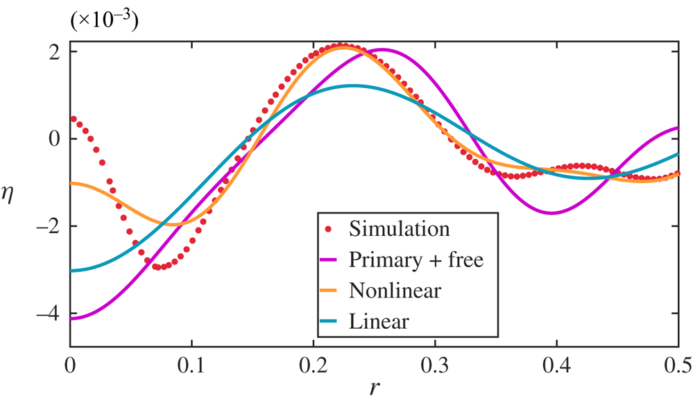
The above exercise can also be carried out when the initial interface deformation takes the shape of a cavity. For this initial condition,  $\eta (r,0) = \sum _{m=1}^{\infty } \eta _m(0) \textrm {J}_0(k_m r)$, as previously shown in figure 5(a). From the numerical solution to (2.6), the temporal frequency spectrum at $r=0$ is obtained. We track the time series generated by $\eta _m(t)$ and eliminate the frequencies $2\omega _m$ and $0$ from its Fourier spectrum. Figure 16 demonstrates that after the removal of these bound modes, the interface (labelled ‘primary + free’) fails to capture the dimple shape. In contrast, the full numerical solution to (2.6) faithfully reproduces the dimple. (We gratefully acknowledge an anonymous referee for several technical clarifications in this section.)
Shape of a dimple for a cavity with  $\varepsilon = 0.091$.

3.4. Viscous effects: comparison with linear theory
In this section, we analyse viscous effects for the chosen initial condition. Using cylindrical coordinates, Miles (Reference Miles1968) solved the problem of free-surface waves on a viscous liquid in the linear regime within a radially unbounded domain for a continuous spectrum of wavenumbers in the radial direction. Farsoiya et al. (Reference Farsoiya, Mayya and Dasgupta2017) extended this theory to internal waves, considering viscosity and density due to both upper and lower fluids, for a single wavenumber in the initial spectrum. Due to the availability of superposition in the linear regime, the results of Farsoiya et al. (Reference Farsoiya, Mayya and Dasgupta2017) are easily extended to initial excitations with multiple wavenumbers. In Cartesian geometry, the single wavenumber initial excitation case was first explicitly studied by Prosperetti (Reference Prosperetti1976) treating free-surface waves and by Prosperetti (Reference Prosperetti1981) treating internal waves. In the Laplace domain and in cylindrical axisymmetric coordinates, the solution to the evolution of a single initial wavenumber  $k_m$ was shown in Farsoiya et al. (Reference Farsoiya, Mayya and Dasgupta2017) to be given by
 \begin{align}
\begin{aligned}
\tilde{\eta}_{m}(s)&=\hat{\eta}_{m}(0)\dfrac{s+\left(4\tilde{k}_m^2\nu-\dfrac{4\tilde{k}_m^3\nu}{\tilde{k}_m+\sqrt{\tilde{k}_m^2+s/\nu}}\right)}{s^2+\left(4\tilde{k}_m^2\nu-\dfrac{4\tilde{k}_m^3\nu}{\tilde{k}_m+\sqrt{\tilde{k}_m^2+s/\nu}}\right)s+\hat{\omega}_m^2},\nonumber\\
&\quad \hat{\omega}_m^2 \equiv g\tilde{k}_m + T\tilde{k}_m^3/\rho,\quad \tilde{k}_m\equiv\dfrac{k_m}{\hat{R}}.\end{aligned}\end{align}
\begin{align}
\begin{aligned}
\tilde{\eta}_{m}(s)&=\hat{\eta}_{m}(0)\dfrac{s+\left(4\tilde{k}_m^2\nu-\dfrac{4\tilde{k}_m^3\nu}{\tilde{k}_m+\sqrt{\tilde{k}_m^2+s/\nu}}\right)}{s^2+\left(4\tilde{k}_m^2\nu-\dfrac{4\tilde{k}_m^3\nu}{\tilde{k}_m+\sqrt{\tilde{k}_m^2+s/\nu}}\right)s+\hat{\omega}_m^2},\nonumber\\
&\quad \hat{\omega}_m^2 \equiv g\tilde{k}_m + T\tilde{k}_m^3/\rho,\quad \tilde{k}_m\equiv\dfrac{k_m}{\hat{R}}.\end{aligned}\end{align}Employing linear superposition, the corresponding (dimensional) expression for the interface evolution in the time domain for the current case becomes
 \begin{equation} \hat{\eta}(\hat{r},\hat{t})= \sum_{m=1}^{17}\hat{\eta}_m(\hat{t}){\mathrm{J}}_{0}\left(k_m\frac{\hat{r}}{\hat{R}}\right),\quad \hat{\eta}_m(\hat{t})\equiv \mathcal{L}^{{-}1}\left[\tilde{\eta}_m(s)\right]. \end{equation}
Here  $\mathcal {L}^{-1}$ is the inverse Laplace operator. We stress that (3.7) accounts for dissipation in the bulk liquid and boundary layer, as demonstrated by Prosperetti (Reference Prosperetti1976) in Cartesian coordinates and by Farsoiya et al. (Reference Farsoiya, Mayya and Dasgupta2017) in cylindrical coordinates. Equation (3.8) is compared with DNS for two different values of $\varepsilon$ and $Oh$ in figures 17 and 18, where inverse Laplace transforms were performed using the Cohen method by Henri Cohen & Zagier (Reference Henri Cohen and Zagier2000) which is a default method in mpmath (2023), a free Python library for arbitrary-precision floating-point arithmetic; see Kayal (Reference Kayal2024) for the code. Figure 17 benchmarks the theory at a relatively small $\varepsilon = 0.006$, where linear viscous theory is expected to be accurate. Excellent agreement with linear viscous theory is observed in figure 17. Conversely, figure 18 shows a clear distinction between linear and nonlinear predictions.
Viscous DNS (indicated as ‘simulation’ with red dots in the legend to panel (a)) with  $\varepsilon =0.006$ and $Oh = 1.17\times 10^{-3}$ corresponding to Case $10$ in table 1. One notes the excellent agreement with linear, viscous theory (blue line, ‘linear’, (3.8) in text) with hardly any nonlinear contribution.

Viscous DNS (indicated as ‘simulation’ with red dots in the legend to panel (a)) with  $\varepsilon =0.091$ and $Oh = 1.17\times 10^{-4}$ corresponding to Case $4$ in table 1. In contrast to figure 17, increasing the value of $\varepsilon$ and a corresponding reduction in viscosity, has a dramatic effect in the simulations. We note that viscous linear theory is no longer adequate particularly during the focussing process in (f–h). In (h), we also provide a comparison of the interface at this time instant, for the inviscid numerical simulation ( $Oh=0$) with the same $\varepsilon$. It is seen that the viscous simulation has a crest which at the indicated instant of time, is taller than the one obtained from the inviscid simulation.
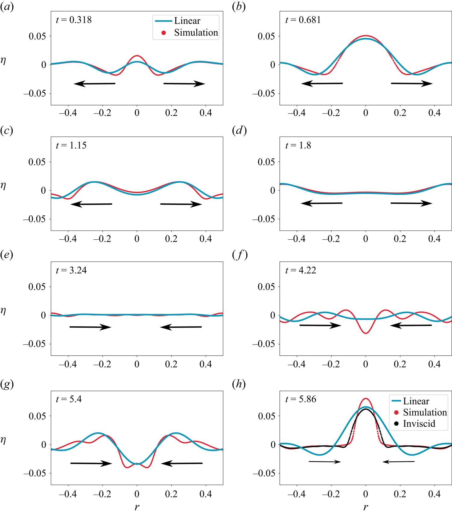
To further investigate the impact of viscosity, figure 19(a) presents the interfacial velocity at  $r=0$ from DNS for various $Oh$ values while figure 19(b) represents the interface displacement at $r=0$, in the same time window. The most notable observation is that the peak velocity at $r=0$ during wave focussing occurs in the viscous simulation rather than the inviscid one. This non-monotonic behaviour as a function of the Ohnesorge number is a well-known phenomenon in other contexts (Duchemin et al. Reference Duchemin, Popinet, Josserand and Zaleski2002; Ghabache et al. Reference Ghabache, Antkowiak, Josserand and Séon2014a), indicating a significant effect of viscosity. In our analysis of converging waves, we attribute the observed non-monotonic behaviour to viscous dissipation within the boundary layer at the gas–liquid interface. Even as the Ohnesorge number approaches zero ( $Oh = 0^+$), this boundary layer remains significant, similar to the dissipative anomaly seen in fully developed turbulence (Prandtl Reference Prandtl1904; Onsager Reference Onsager1949; Eggers Reference Eggers2018; Dubrulle Reference Dubrulle2019) and recently explored in contexts such as sheet retraction (Sanjay et al. Reference Sanjay, Sen, Kant and Lohse2022) and drop impact (Sanjay, Chantelot & Lohse Reference Sanjay, Chantelot and Lohse2023; Sanjay & Lohse Reference Sanjay and Lohse2024) interfacial flows. Consequently, this non-zero viscous dissipation intensifies the focussing of capillary waves, thereby increasing the velocity at the centre ( $r = 0$). To validate this hypothesis, in the next section, we next employ the viscous potential flow approach, which accounts for bulk viscous dissipation but neglects dissipation in the gas–liquid boundary layer, to model the converging waves.
(a) Velocity at the interface at  $\hat {r}=0$ for different values of $Oh$ and fixed $\varepsilon = 0.091$. Note that the viscous DNS for $Oh = 1.17\times 10^{-4}$ (solid deep blue line) produces the largest velocity peak around $t\approx 5.7$. Note in particular that the inviscid signal ( $Oh=0$, red symbols) has a peak which is shorter by a factor of half. This difference is because in the $Oh=0$ case, we are not resolving the numerically generated boundary layer at the current grid resolution. As discussed in the text, this introduces a degree of grid dependency in the inviscid simulations which cannot be resolved in the numerical framework of the open-source code Basilisk (Popinet & Collaborators Reference Popinet2013–2024). However, for $Oh\geq 1.17\times 10^{-4}$, we are resolving the boundary layers and the results are grid convergent. (b) The interface height $\eta (0,t)$ with the same colour scheme as in (a). We refer the reader to Appendix C where the grid convergence results for this (and other) simulations are provided.

We emphasise that DNS for  $Oh < 1.17 \times 10^{-4}$ exhibit grid dependency, as indicated by the pink shaded region in figure 21(a,b). This dependency arises from insufficient grid resolution to properly resolve the boundary layer in low-viscosity liquids, a challenge analogous to those encountered in wall-bounded turbulence studies (Lohse & Shishkina Reference Lohse and Shishkina2024) and classical contact line simulations (Snoeijer & Andreotti Reference Snoeijer and Andreotti2013). These fields continue to grapple with resolving multiple scales spanning orders of magnitude. We designate this unresolved region in pink, highlighting an open problem for future multiscale simulations. The $Oh=0$ simulation, represented by symbols in figure 19(a), demonstrates grid dependency in velocity at $r=0$ for resolutions up to $2048^2$ (maximum adaptive level). This manifests as isolated ‘spike’ points in figure 24(a). In contrast, the nonlinear analytical prediction, depicted by the green curve labelled ‘ $N$’ in figure 19(a), does not exhibit such spikes. In the (inviscid) Euler limit, our results align with inviscid nonlinear theory (see figures 9 and 10). However, we stress that this scenario also exhibits grid dependency. The one-fluid approximation used in Basilisk to solve Euler equations creates an over-constrained system by enforcing continuity of tangential velocity at the gas–liquid interface, which is incompatible with Euler equations. Consequently, indefinite grid refinement generates deviations, as evident in figure 24(a). Lastly, despite setting $Oh = 0$, our simulations retain a non-zero, grid-dependent viscosity. These factors should be considered when interpreting comparisons between inviscid, potential flow theory (where tangential velocity at the interface is discontinuous) and our numerical results obtained from Basilisk.
3.5. Viscous potential flow
To further elucidate viscous effects, we incorporate viscosity into the nonlinear equations using the viscous potential flow (VPF) model (Joseph Reference Joseph2006). Unlike the linear case discussed previously, this method does not account for the boundary layer formed at the free surface, since it does not enforce the zero shear stress boundary condition (Moore Reference Moore1963). As is well known, in this approach the normal stress boundary condition (2.1c) is modified to incorporate the effect of bulk viscous damping to obtain
 $$\begin{gather} \left(\frac{\partial\phi}{\partial t}\right)_{z=\eta}+\eta+2\;b\;Oh\; \sqrt{\alpha}\; \left(\frac{\partial^2\phi}{\partial z^2}\right)_{z=\eta}+\frac{1}{2}\left\{\left(\frac{\partial\phi}{\partial r}\right)^2+\left(\frac{\partial\phi}{\partial z}\right)^2\right\}_{z=\eta} \nonumber\\ -\;\alpha\left(\frac{\partial^2\eta}{\partial r^2}+\frac{1}{r}\frac{\partial\eta}{\partial r}\right) =0. \end{gather}$$
We follow the same strategy as the inviscid case and obtain a modified differential equation for  $\eta _n$, i.e. the viscous counterpart of (2.6) leading to
 \begin{align} &\dfrac{{\rm d}^2\eta_n}{{\rm d} t^2}+\omega_n^2\eta_n+2\;b\;Oh\; \sqrt{\alpha}\; k_n^2 \frac{{\rm d}\eta_n}{{\rm d}t}+2b\;Oh\;\sqrt{\alpha}\; k_n \sum_{m,p} k_m^2 C_{npm} \frac{{\rm d}\eta_m}{{\rm d}t}\eta_p \nonumber\\ &\qquad + k_n\sum_{m,p}\left[1+\frac{k_p^2-k_m^2-k_n^2}{2k_mk_n}\right]C_{npm}\left(\dfrac{{\rm d}^2\eta_m}{{\rm d} t^2}\right)\eta_p \nonumber\\ &\qquad +\dfrac{1}{2}k_n\sum_{m,p}\left[1+\dfrac{k_p^2+k_m^2-k_n^2}{2k_mk_p}+\dfrac{k_p^2-k_m^2-k_n^2}{k_mk_n}\right]C_{npm}\left(\dfrac{{\rm d}\eta_m}{{\rm d} t}\right)\left(\frac{{\rm d}\eta_p}{{\rm d} t}\right)=0. \end{align}
 In figure 20, we compare the nonlinear analytical inviscid solution (referred to as ‘inviscid’ in the legend), the VPF solution for  $\varepsilon = 0.091$ and the viscous DNS (referred to as ‘simulation’) for Case $4$ in table 1. It is seen that the VPF solution, is indistinguishable from the inviscid one in the limit of $Oh = 0^+$, highlighting the importance of resolving the viscous boundary layer in theory.
Comparison of the VPF (black dotted line), inviscid solution (green solid line) and DNS (red dots) at  $\varepsilon =0.091$ and $Oh=1.17\times 10^{-4}$, Case $4$ in table 1.
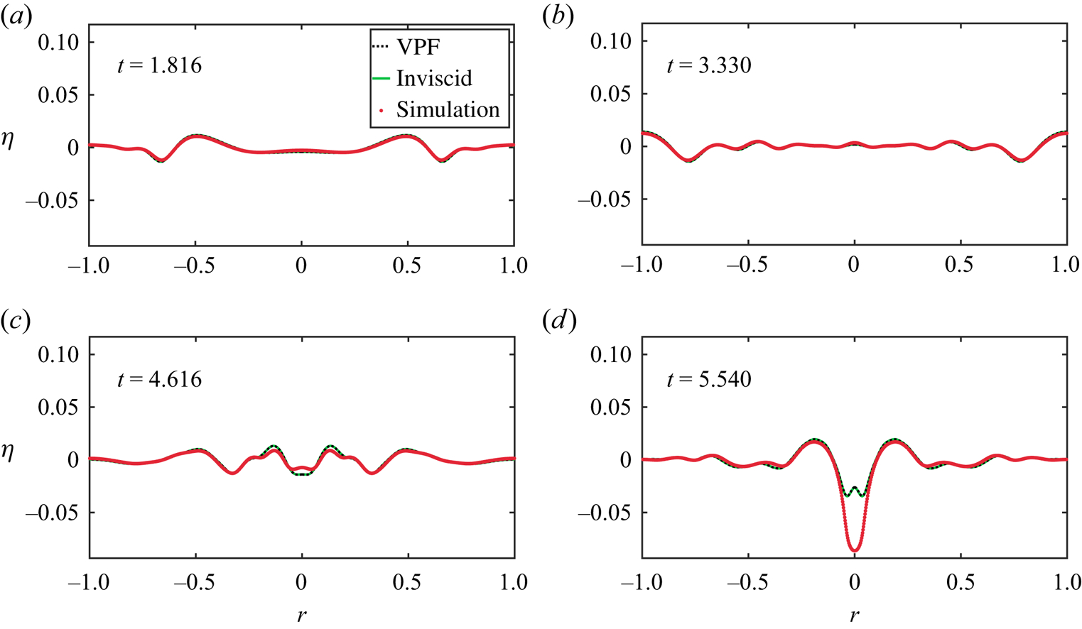
To further quantify the comparison between these cases, in figure 21(a) shows the maximum velocity at the axis of symmetry within a shallow cavity during focussing. The linear viscous theory, which accounts for the boundary layer at the free surface, describes the change in  $v_z$ with Ohnesorge number slightly better than the VPF model. Figure 21(b) presents results for a deeper cavity where nonlinearity plays a significant role, and the non-monotonic behaviour observed in figure 19(a) as a function of $Oh$ is evident. The VPF model fails to capture this non-monotonic behaviour, highlighting the importance of resolving the boundary layer at the gas–liquid interface, as discussed in § 3.4. We propose developing a nonlinear-viscous theory superior to the VPF model to explain the observations in figures 19 and 21(b) in future work.
Comparison of the maximum velocity at  $r=0$, i.e. $v_z^{max}$ (see arrows in figure 19a) after reflection for different Ohnesorge number for a shallow cavity, Cases $7,9,10,11,12$ in table 1 (panel (a)) and for a deep cavity, Cases $2,4,5,6,13,14$ (panel (b)). In (a) the ‘+’ symbols represent DNS with finite viscosity. Black dotted line represents DNS with zero viscosity. Red symbols represent the linear viscous solution obtained by numerical inversion of (3.7). Green symbols indicate VPF approximation obtained from solving (3.10). At the $Oh=0$ limit, VPF (green dashed line) and linear viscous theory (red dashed line) coincide with the linear inviscid theory (blue dashed line). In panel (b) the symbols have the same meaning as in (a), the only difference is that we have employed nonlinear inviscid theory (blue dashed line) in this case. Note that non-monotonicity in the velocity at $r=0$ as a function of $Oh$. The VPF approximation despite being nonlinear is unable to describe this non-monotonicity, presumably because of its inability to resolve the boundary layer at the free surface. The dotted black line represents the velocity of inviscid DNS which shows grid dependency. In the current figure, below a certain value of $Oh$ (pink shaded region) grid dependency persists in our simulations, due to the presence of an unresolved thin boundary layer. We do not depict this data here due to the lack of this convergence. For $Oh > 1.17\times 10^{-4}$, however, the boundary layers are resolved for simulation points ‘+’ and the data are grid converged. Note that the nonlinear inviscid theory ( $Oh=0$, dashed blue line) predicts $v_z^{max}(r=0)$ which is smaller than the prediction by DNS for $Oh\approx 1.17\times 10^{-4}$ by a factor $\approx 2$. A similar albeit significantly more intensification at an optimal value of $Oh$ was first noted in the case of bubble bursting in the seminal study by Duchemin et al. (Reference Duchemin, Popinet, Josserand and Zaleski2002); see their figure 12. Here (a) shallow cavity with $\varepsilon = 0.006$; (b) deep cavity with $\varepsilon =0.091$.
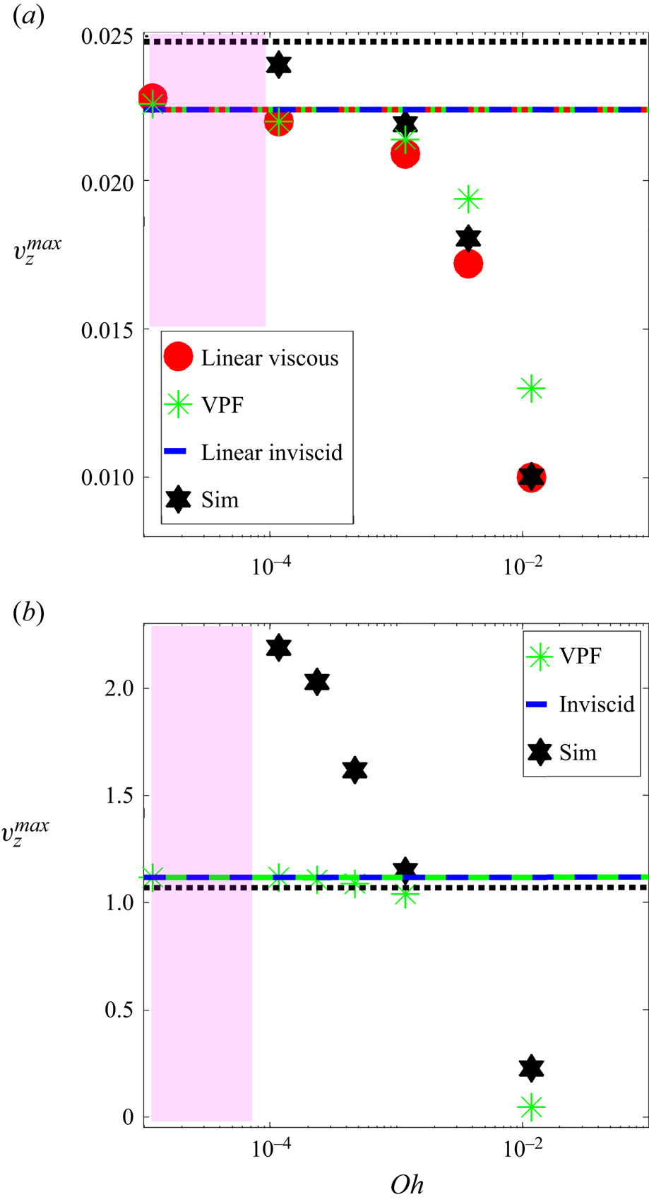
4. Conclusion and outlook
In this study, we have discussed the dynamics of a localised free-surface perturbation in a cylindrical pool of liquid, which generates a train of waves. These waves, upon reflecting from the container walls, converge back towards the axis of symmetry, leading to progressively increasing free-surface oscillations at the centre. Using the potential flow approximation, we derived a set of ODEs governing the evolution of amplitudes up to second order.
For shallow cavities, linear theory suffices to explain the wave evolution. However, as the cavity depth increases, the limitations of linear theory become evident, particularly in predicting the focussing effects at  $r=0$. Our findings demonstrate that linear dispersive focussing alone is inadequate to describe the intricate dimple shape forming at the axis of symmetry for deeper cavities. A nonlinear theory that accounts for the generation of bound components is found to be essential for accurately modelling the focussing process. The role of bound components is particularly critical in capturing the interface evolution at the symmetry axis.
A notable observation is the significant influence of viscosity on the focussing process. Interestingly, the maximum velocity at the axis of symmetry is higher for a slightly viscous fluid than for an inviscid one. This non-monotonic behaviour with respect to the Ohnesorge number  $Oh$ is not captured by either the linear viscous model (Prosperetti Reference Prosperetti1976; Farsoiya et al. Reference Farsoiya, Mayya and Dasgupta2017) or the nonlinear VPF model (Joseph Reference Joseph2006). The VPF model's failure, stemming from its neglect of boundary layer effects, underscores the critical role of these layers in the $Oh \to 0^+$ limit. As the VPF model converges to an inviscid solution in this limit, it further emphasises the boundary layers’ importance in velocity enhancement. The singular nature of the $Oh \to 0^+$ limit arises from fundamental disparities between Navier–Stokes and Euler equations. Even as $Oh$ approaches zero, the no-slip condition at the liquid–gas interface necessitates a boundary layer, preserving viscous effects.
In conclusion, we emphasise some interesting observations and hypothesis made in Zhang & Thoroddsen (Reference Zhang and Thoroddsen2008) concerning capillary wave focussing, albeit on a spherical bubble unlike the flat surface treated here. Some of these find qualitative support from our theory. In page  $9$, first column, first paragraph of Zhang & Thoroddsen (Reference Zhang and Thoroddsen2008), the authors remark insightfully that the wave convergence process is itself not necessarily nonlinear, as the large amplitude oscillations seen in their figure 14 are also predicted by linear theory. However, linear amplification itself may not be enough to trigger pinch-off, emphasising the local importance of nonlinearity at the focal point. Our analysis establishes that this is qualitatively true, cf. figure 18. In their section C (p. 9), Zhang & Thoroddsen (Reference Zhang and Thoroddsen2008) also emphasise that the phase and amplitude of the wavetrain is very important to the convergence process. Our nonlinear analysis establishes the importance of the amplitude of the wavetrain while the viscous analysis demonstrates that the VPF model (which does not resolve the interface boundary layer) is unable to capture the non-monotonic dependence of vertical velocity at $r=0$ on $Oh$. Presumably, this non-monotonicity will be predicted from a nonlinear, viscous model, which is still simpler than the full Navier–Stokes equation and this is proposed as future work. Upcoming research thus needs to develop a comprehensive, nonlinear viscous theory that incorporates boundary layer effects and also accounts for the nonlinearity associated with focussing. Additionally, extending this work to non-Newtonian fluids, such as viscoplastic or viscoelastic liquids (Sanjay, Lohse & Jalaal Reference Sanjay, Lohse and Jalaal2021), could reveal new insights and broaden the applicability of our theoretical framework.
Supplementary material
Supplementary movies are available at https://doi.org/10.1017/jfm.2024.1089. Movie 1, comparison of cavity evolution at  $\varepsilon =0.61$; movie 2, inviscid DNS of cavity evolution at $\varepsilon =0.91$. All codes are available at Kayal (Reference Kayal2024).
Acknowledgements
R.D. thanks Professor B. Sutherland for sharing the study by Smith (Reference Smith1976). V.S. thanks Professor D. Lohse for stimulating discussions on viscous anomaly.
Funding
We gratefully acknowledge financial support from DST-SERB (Government of India) grants MTR/2019/001240, CRG/2020/003707 and SPR/2021/000536 on topics related to waves, jet formation, cavity collapse and the viscous Cauchy–Poisson problem. The PhD tenure of L.K. is supported by the Prime-Minister's Research Fellowship (PMRF), Government of India and is gratefully acknowledged. V.S. acknowledges funding from NWO and Canon under the project FIP-II.
Declaration of interests
The authors report no conflict of interest.
Appendix A
The expressions for the third-order approximation to  $\eta (r, \tilde {t};\tilde {\epsilon })$ by Mack (Reference Mack1962) expressed in our notation are
 \begin{align} T_0(r;\tilde{\epsilon}) &\equiv \frac{1}{4} \tilde{\epsilon}^2 k_1({\rm J}_{01}^2 - {\rm J}_{11}^2), \end{align}
 \begin{align} T_1(r;\tilde{\epsilon}) &\equiv \tilde{\epsilon} {\rm J}_{01} + \frac{\tilde{\epsilon}^3 k_1^2 }{4} \left\{\vphantom{\sum_{j=1}^\infty \frac{k_j^2 \varGamma_j\alpha_n[{\rm J}_{11}{\rm J}_{1j}]}{k_1^2}} {\rm J}_{01}^3 - \frac{5}{2} {\rm J}_{01} {\rm J}_{11}^2 \right.\nonumber\\ &\quad + \frac{{\rm J}_{11}^3}{k_1 r} + \frac{1}{8} \sum_{i=1}^\infty \frac{k_{i}\varGamma_i {\rm J}_{01}{\rm J}_{0i}}{k_1} - \frac{1}{4} \sum_{i=1}^\infty \frac{k_{i}^2\varGamma_i {\rm J}_{01}{\rm J}_{0i}}{k_1^2} - \sum_{i=1}^\infty \frac{1}{8}\frac{k_{i}^2\varGamma_i {\rm J}_{11}{\rm J}_{1i}}{k_1^2} \nonumber\\ &\quad + \frac{1}{4} \sum_{i=1}^\infty \frac{k_{i}\varGamma_i {\rm J}_{01}{\rm J}_{0i}}{k_1} + \sum_{i=2}^\infty \frac{(k_i/k_1){\rm J}_{0i}}{1 - (k_i/k_1)} \left[\vphantom{\sum_{j=1}^\infty \frac{k_j^2 \varGamma_j\alpha_n[{\rm J}_{11}{\rm J}_{1j}]}{k_1^2}} - \alpha_n[{\rm J}_{01}^3] -\alpha_n[{\rm J}_{01}{\rm J}_{11}^2] \right.\nonumber\\ &\quad + \alpha_n\left[\frac{{\rm J}_{11}^3}{k_1 r}\right] -\frac{1}{4}\sum_{j=1}^\infty \frac{k_j^2 \varGamma_j \alpha_n[{\rm J}_{01}{\rm J}_{0j}]}{k_1^2} + \frac{1}{2}\sum_{j=1}^\infty \frac{k_j \varGamma_j \alpha_n[{\rm J}_{01}{\rm J}_{0j}]}{k_1} \nonumber\\ &\left.\left.\quad -\frac{1}{8}\sum_{j=1}^\infty \frac{k_j^2 \varGamma_j\alpha_n[{\rm J}_{11}{\rm J}_{1j}]}{k_1^2} \right] \right\}, \end{align}
 \begin{align} T_2(r;\tilde{\epsilon}) &\equiv \frac{\tilde{\epsilon}^2 k_1}{4} \left( {\rm J}_{01}^2 -{\rm J}_{11}^2 - \frac{1}{4}\sum_{i=1}^\infty \frac{k_i \varGamma_i {\rm J}_{0i}}{k_1} \right), \end{align}
 \begin{align} T_3(r;\tilde{\epsilon})
&\equiv \frac{\tilde{\epsilon}^3 k_1^2}{12} \left(\vphantom{\sum_{j=1}^\infty \frac{k_j \varGamma_j
\alpha_n[{\rm J}_{11}{\rm J}_{1j}]}{k_1}} {\rm
J}_{01}^3 - \frac{7}{2}{\rm J}_{01}{\rm J}_{11}^2 +
\frac{{\rm J}_{11}^3}{k_1 r} - \frac{1}{8}
\sum_{i=1}^\infty \frac{k_{i}\varGamma_i {\rm J}_{01}{\rm
J}_{0i}}{k_1} \right.\nonumber\\ &\quad - \frac{1}{4}
\sum_{i=1}^\infty \frac{k_{i}^2\varGamma_i {\rm J}_{01}{\rm
J}_{0i}}{k_1^2} + \sum_{i=1}^\infty
\frac{1}{8}\frac{k_{i}^2\varGamma_i {\rm J}_{11}{\rm
J}_{1i}}{k_1^2} \nonumber\\ &\quad +\frac{1}{4}
\sum_{i=1}^\infty \frac{k_{i}\varGamma_i {\rm J}_{01}{\rm
J}_{0i}}{k_1} -\frac{1}{9}\sum_{i=1}^\infty
\frac{(k_i/k_1){\rm J}_{0i}}{1 - (k_i/9k_1) }
\left[\vphantom{\sum_{j=1}^\infty \frac{k_j \varGamma_j
\alpha_n[{\rm J}_{11}{\rm J}_{1j}]}{k_1}} 5\alpha_n[{\rm
J}_{01}^3] + \frac{7}{2}\alpha_n[{\rm J}_{01}{\rm
J}_{11}^2]\right. \nonumber\\ &\quad
-\alpha_n\left[\frac{{\rm J}_{11}^3}{k_1 r}\right] -
\frac{5}{2}\sum_{j=1}^\infty \frac{k_j \varGamma_j
\alpha_n[{\rm J}_{01}{\rm J}_{0j}]}{k_1} +
\frac{1}{4}\sum_{j=1}^\infty \frac{k_j^2 \varGamma_j
\alpha_n[{\rm J}_{01}{\rm J}_{0j}]}{k_1^2} \nonumber\\
&\left.\left.\quad + \frac{1}{8}\sum_{j=1}^\infty
\frac{k_j^2 \varGamma_j \alpha_n[{\rm J}_{11}{\rm
J}_{1j}]}{k_1^2} - \sum_{j=1}^\infty \frac{k_j \varGamma_j
\alpha_n[{\rm J}_{11}{\rm J}_{1j}]}{k_1} \right] \right).
\end{align}
\begin{align} T_3(r;\tilde{\epsilon})
&\equiv \frac{\tilde{\epsilon}^3 k_1^2}{12} \left(\vphantom{\sum_{j=1}^\infty \frac{k_j \varGamma_j
\alpha_n[{\rm J}_{11}{\rm J}_{1j}]}{k_1}} {\rm
J}_{01}^3 - \frac{7}{2}{\rm J}_{01}{\rm J}_{11}^2 +
\frac{{\rm J}_{11}^3}{k_1 r} - \frac{1}{8}
\sum_{i=1}^\infty \frac{k_{i}\varGamma_i {\rm J}_{01}{\rm
J}_{0i}}{k_1} \right.\nonumber\\ &\quad - \frac{1}{4}
\sum_{i=1}^\infty \frac{k_{i}^2\varGamma_i {\rm J}_{01}{\rm
J}_{0i}}{k_1^2} + \sum_{i=1}^\infty
\frac{1}{8}\frac{k_{i}^2\varGamma_i {\rm J}_{11}{\rm
J}_{1i}}{k_1^2} \nonumber\\ &\quad +\frac{1}{4}
\sum_{i=1}^\infty \frac{k_{i}\varGamma_i {\rm J}_{01}{\rm
J}_{0i}}{k_1} -\frac{1}{9}\sum_{i=1}^\infty
\frac{(k_i/k_1){\rm J}_{0i}}{1 - (k_i/9k_1) }
\left[\vphantom{\sum_{j=1}^\infty \frac{k_j \varGamma_j
\alpha_n[{\rm J}_{11}{\rm J}_{1j}]}{k_1}} 5\alpha_n[{\rm
J}_{01}^3] + \frac{7}{2}\alpha_n[{\rm J}_{01}{\rm
J}_{11}^2]\right. \nonumber\\ &\quad
-\alpha_n\left[\frac{{\rm J}_{11}^3}{k_1 r}\right] -
\frac{5}{2}\sum_{j=1}^\infty \frac{k_j \varGamma_j
\alpha_n[{\rm J}_{01}{\rm J}_{0j}]}{k_1} +
\frac{1}{4}\sum_{j=1}^\infty \frac{k_j^2 \varGamma_j
\alpha_n[{\rm J}_{01}{\rm J}_{0j}]}{k_1^2} \nonumber\\
&\left.\left.\quad + \frac{1}{8}\sum_{j=1}^\infty
\frac{k_j^2 \varGamma_j \alpha_n[{\rm J}_{11}{\rm
J}_{1j}]}{k_1^2} - \sum_{j=1}^\infty \frac{k_j \varGamma_j
\alpha_n[{\rm J}_{11}{\rm J}_{1j}]}{k_1} \right] \right).
\end{align}
The  $O(\tilde {\epsilon }^3)$ accurate, nonlinear frequency $\omega (\tilde {\epsilon },q=1)$ is given by
 \begin{align} \omega^2(\tilde{\epsilon},q=1) &= k_1 \left\{ 1 + \frac{\tilde{\epsilon}^2 k_1^4}{4}\left( -\alpha_1[{\rm J}_{01}^3] - \alpha_1[{\rm J}_{01} {\rm J}_{11}^2] + \alpha_1\left[\frac{{\rm J}_{11}^3}{k_1 r}\right] - \frac{1}{4} \sum_{i=1}^\infty \frac{k_{i}^2\varGamma_i {\rm J}_{01} {\rm J}_{0i}}{k_1^2} \right.\right.\nonumber\\ &\left.\left.\quad + \frac{1}{2}\sum_{i=1}^\infty \frac{k_i \varGamma_i \alpha_1[{\rm J}_{01} {\rm J}_{0i}]}{k_1} - \frac{1}{8}\sum_{i=1}^\infty \frac{k_i^2 \varGamma_i \alpha_1[{\rm J}_{11} {\rm J}_{1i}]}{k_1} \right) \right\} \end{align}
with the functionals  $\alpha [{\cdot }]$ and $\gamma [{\cdot }]$ defined as
 \begin{equation} \alpha_n\left[F(r)\right] \equiv \frac{\int_0^1 r F(r) {\rm J}_{0n} \,{\rm d}r}{\dfrac{1}{2} ({\rm J}_0(k_{n}))^2},\quad \varGamma_i\left[F(r)\right] \equiv \frac{2 \alpha_n[ {\rm J}_{01}^2 ] + 2 \alpha_n[ {\rm J}_{11}^2 ] }{1 - \dfrac{k_n}{4k_1}}. \end{equation}
We have used the definitions  ${\rm J}_1(k_n) = 0 (n=1,2,3,\ldots )$ and the shorthand notation ${\rm J}_{ij} = {\rm J}_i(k_j r)$.
Appendix B
We derive the relation between the nonlinear interaction coefficients  $C_{mnq}$ and $D_{mnq}$ discussed in (2.5). This relation has been provided in Nayfeh (Reference Nayfeh1987) and Miles (Reference Miles1976) without proof and the same is presented here. Following Nayfeh (Reference Nayfeh1987), we represent (2.1) a in (semi) basis-independent notation as
 \begin{equation} \phi(\boldsymbol{x},z,t) = \sum_{m=1}^{\infty}\phi_m(t)\varPsi_m(\boldsymbol{x})\exp(k_mz), \end{equation}
where  $\boldsymbol {x}$ is the horizontal position vector and $\varPsi _m$ satisfies the equation $\nabla _H^2\varPsi _m + k_m^2 \varPsi = 0$ as a consequence of $\phi$ satisfying the Laplace equation; note that $\nabla ^2 = \nabla _H^2 + {\partial ^2}/{\partial z^2}$. We assume that $\varPsi _m(\boldsymbol {x})$ follow the orthogonality rule $\iint \, {\rm d}S\;\psi _m(\boldsymbol {x})\psi _q(\boldsymbol {x}) = \delta _{mq}S$ where $\delta _{mq}$ is the Kronecker delta. Using Stokes theorem to relate an area integral (over $s$) in two dimensions to the line integral, we have for a vector field $\boldsymbol {F}(\boldsymbol {x})$
 \begin{equation} \iint \,{\rm d}s\;\boldsymbol{\nabla}_H\boldsymbol{\cdot}\boldsymbol{F} = \int \,{\rm d}l\left(\boldsymbol{F}\boldsymbol{\cdot}\boldsymbol{n}\right). \end{equation}
Choosing  $\boldsymbol {F} = \psi _q\psi _{m}\boldsymbol {\nabla }_H\psi _n$, (B2) leads to
 \begin{equation} \iint \left[\psi_q\left(\boldsymbol{\nabla}_H\psi_m\boldsymbol{\cdot}\boldsymbol{\nabla}_H\psi_n\right) + \psi_m\left(\boldsymbol{\nabla}_H\psi_q\boldsymbol{\cdot}\boldsymbol{\nabla}_H\psi_n\right) + \psi_q\psi_m\nabla_H^2 \psi_n\right]\,{\rm d}s = 0, \end{equation}
the right-hand side following from the no-penetration condition at the wall. Following the same notation as Nayfeh (Reference Nayfeh1987), we define
 \begin{equation} \iint\,{\rm d}s\; \psi_m(\boldsymbol{x})\psi_n(\boldsymbol{x})\psi_q(\boldsymbol{x}) \equiv S\;C_{mnq},\quad \iint\,{\rm d}s\; \left(\boldsymbol{\nabla}_H\psi_m(\boldsymbol{x})\boldsymbol{\cdot}\boldsymbol{\nabla}_H\psi_n(\boldsymbol{x})\right)\psi_q(\boldsymbol{x}) \!\equiv\! S\;D_{mnq}.\end{equation}
Note that  $D_{nmq} = D_{mnq}$. Using (B4), (B3) may be written compactly as
 \begin{equation} D_{mnq} + D_{qnm} - k_n^2C_{mnq} = 0. \end{equation}
Replacing  $m\rightarrow n, n\rightarrow q, q\rightarrow m$ in (B5), we obtain
 \begin{equation} D_{nqm} + D_{mqn} - k_q^2C_{nqm} = 0, \end{equation}
which may be rewritten as
 \begin{equation} D_{qnm} + D_{qmn} - k_q^2C_{nqm} = 0. \end{equation}
 \begin{equation} D_{mnq} = k_n^2C_{mnq} - \left(k_q^2C_{nqm} - D_{qmn}\right). \end{equation}
Replacing once again  $m\rightarrow q, n\rightarrow m, q\rightarrow n$ in (B5), we obtain
 \begin{equation} D_{qmn} + D_{nmq} - k_m^2C_{qmn} = 0. \end{equation}
Combining (B8) and (B9) and the fact that  $D_{mnq} = D_{nmq}$, we obtain
 \begin{equation} D_{nmq} = \frac{1}{2}\left(k_n^2 + k_m^2 - k_q^2\right)C_{nmq}. \end{equation}
After some manipulation, (2.5) follows from the above expression.
Appendix C
Figures 22 and 23 illustrate grid convergence results at three resolutions ( $512^2$, $1024^2$ and $2048^2$) for Cases 4 and 2, respectively, from table 1. Figure 24(a,b) present grid convergence for the velocity at the symmetry axis.
Comparison of interface profile for Case  $4$ in table 1 at three different grid resolutions, $512^2$ (blue dots), $1024^2$ (red dots) and $2048^2$ (green dots).
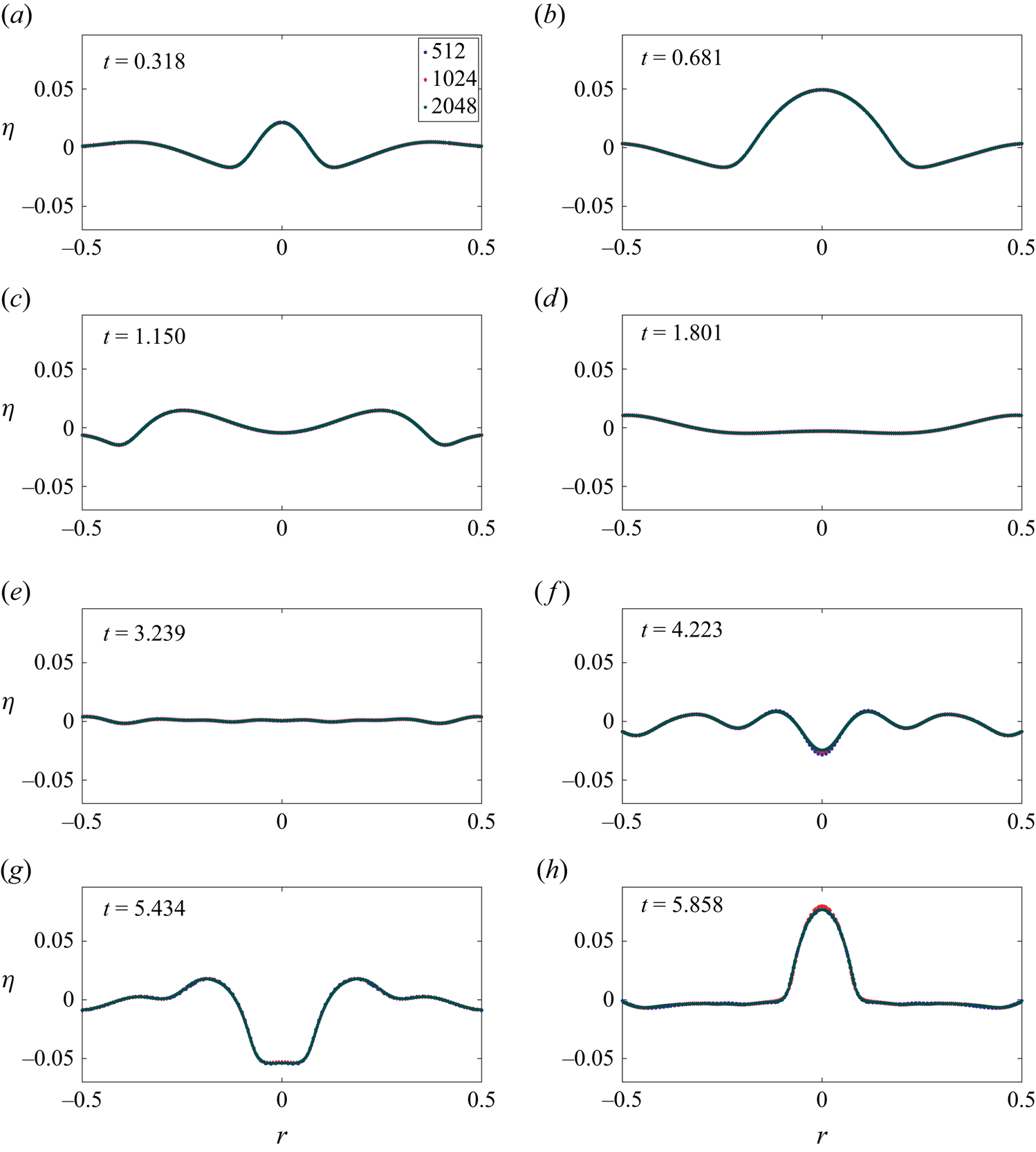
Comparison of interface profile for Case  $2$ in table 1 for three different grid resolutions, $512^2$ (blue dots), $1024^2$ (red dots) and $2048^2$ (green dots).

Comparison of the vertical velocity for Case 2 (panel (a)) and Case 4 (panel (b)) for three different grid resolutions,  $512^2$ (red solid line), $1024^2$ (blue solid line) and $2048^2$ (green solid line). In (a), we also provide the prediction from the numerical solution to the analytical model from (2.6) indicated as ‘N’ in the figure. Here (a) $Oh=0$; (b) $Oh=1.17\times 10^{-4}$.
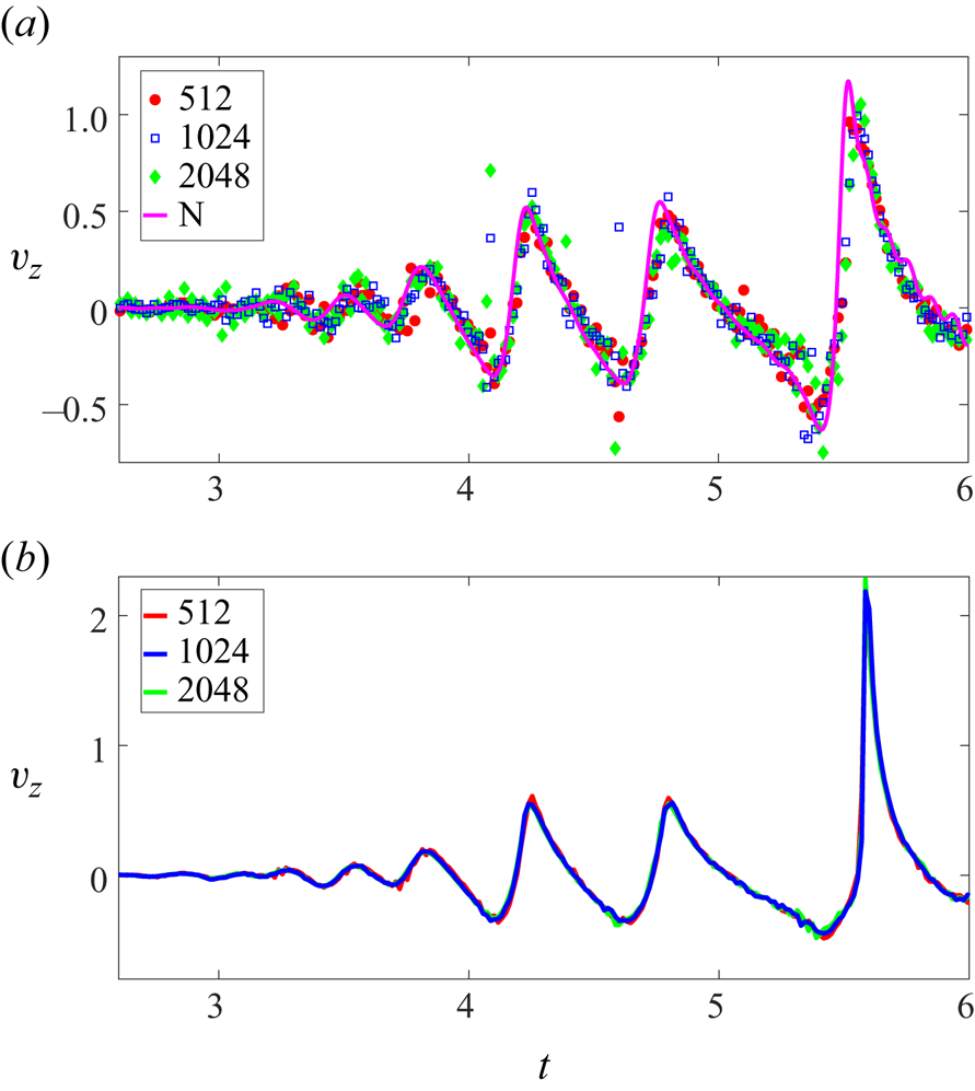
For the inviscid case ( $Oh = 0$, figure 24a), while the overall vertical velocity trend remains consistent, the presence of spikes and the magnitude exhibit grid refinement sensitivity. To provide a robust reference, we include the inviscid, nonlinear analytical solution in figure 24(a) denoted by ‘ $N$’. This demonstrates good agreement with the $Oh = 0$, DNS solution, capturing the main temporal velocity variation features without spurious peaks, thus validating the observed simulation behaviour. As $Oh$ approaches zero, our one-fluid approximation made in the solver Basilisk (Popinet & Collaborators Reference Popinet2013–2024) imposes a no-slip condition at the liquid–gas interface. Resolving this boundary layer requires a minimum grid size of $\Delta \sim KLOh^2$, where $L$ is the characteristic length and $K$ a system-dependent prefactor. This establishes a critical $Oh$ above which results converge well. We empirically determined this as $Oh = 1.17 \times 10^{-4}$ through grid independence testing. Results below this critical value remain unresolved due to insufficient grid resolution, indicated by the pink shaded region in figure 21(b). Further computational method improvements are needed to resolve cases where $Oh < 1.17 \times 10^{-4}$.
Appendix D
Figure 25 depicts the qualitative difference in behaviour starting from a cavity with  $\varepsilon =0.091$ (figure 25a). Here no jet is seen initially and the wavetrain focusses at $r=0$ after some time. In figure 25(b) with $\varepsilon =0.242$, a jet is seen at a much earlier time, and no focussing wavetrain is apparent. In this study, we focus on the regime indicated in figure 25(a). The jet in figure 25(b) is close to the one that was reported in Basak et al. (Reference Basak, Farsoiya and Dasgupta2021), albeit from a single Bessel function.
Both (a) and (b) start with the interface deformed as a cavity shown in red with different  $\epsilon$. Here (a) (red) interface at $t=0$, (green dashed curve) numerical simulation and (blue) linear approximation at $t=0.36T$, when the interface reaches its maximum height and (black curve) at a much later time $t=4.2T$. (b) The same colour code as in (a), (blue) for $t=0.48T$. Here $T$ is the dominant mode time period in the initial spectrum (linear approximation). The arrows in (b) indicate the approximate direction of flow resulting from the initial (capillary) pressure gradient. The jet which was studied in Basak et al. (Reference Basak, Farsoiya and Dasgupta2021) from $\eta (r,t=0)=\varepsilon {\rm J}_0(k_5 r)$ is closely related to the jet in (b). Note the lack of any visible wavetrain when this jet is produced. In this case, pressure difference arising due to the initial steep interface distortion around $r=0$, triggers a radially inward flow towards the same (indicated with arrows in figure 1b). The radial component of this inflow produces a stagnation zone of high pressure at the base of the cavity and a resultant upward jet. We label this situation as ‘flow focussing’. This jet in Basak et al. (Reference Basak, Farsoiya and Dasgupta2021) is associated with a large stagnation pressure at its base, involving conversion of kinetic energy (nonlinear term in Bernoulli equation) to pressure energy. In contrast in (a), no significant stagnation pressure zone develops initially (as the initial cavity is comparatively less steep compared with panel (b)). In this case nonlinear effects become manifest much later when the wavetrain focusses on to the symmetry axis, producing rapid interfacial oscillations at $r=0$. The apparent importance of nonlinearity around $r=0$ in this case is somewhat akin to linear dispersive focussing of surface waves, where nonlinearity becomes locally important at the focal point. Here (a) $\varepsilon =0.091$, wave focussing; (b) $\varepsilon =0.242$, flow focussing.

Appendix E. Comparison with Gordillo & Rodríguez-Rodríguez (Reference Gordillo and Rodríguez-Rodríguez2019)
Although the wavetrain in case of bubble bursting ( $Bo\ll 1$) (Gordillo & Rodríguez-Rodríguez Reference Gordillo and Rodríguez-Rodríguez2019) is different from the one we study here, some qualitative comparisons can be obtained between the two. In this section, we estimate the speed of propagation of the dominant crest for $\varepsilon =0.091$ and $Oh=0$. Similar to the figure 4(b) in Gordillo & Rodríguez-Rodríguez (Reference Gordillo and Rodríguez-Rodríguez2019), we observe that the waves propagating outwards and inwards propagate with the linear speed. This is validated in figure 26 by tracking the local maxima on the free surface in simulations, before and after reflection. In both cases, the propagation speed agrees with the phase speed of the dominant Bessel function ( $k_4$), see figure 5(b). Figure 27 provides an approximate scaling relation (to act as guides only) for the dependence of $v_z$ on $Oh$. We stress that we do not have theoretical description of these power laws and they are distinct from the $v_z^{max} \sim V_\gamma Oh$ established for bursting bubbles for $Oh > Oh_c$. Unlike the case of bubble bursting seen in figure 12 in the seminal study by Duchemin et al. (Reference Duchemin, Popinet, Josserand and Zaleski2002), the intensification seen in $v_z^{max}$ for our case for the optimal $Oh_c$ compared with $Oh\rightarrow 0$ is only approximately a factor of two. In the case of bubble bursting, this factor can be as high as $10$ (Gordillo & Blanco-Rodríguez Reference Gordillo and Blanco-Rodríguez2023). Note that $Oh_c$ appears as a fitting parameter in all existing bursting bubble theories and further work is needed to estimate this value. Our analysis shows that a first-principles theory for this may have to include nonlinearity and also resolve the boundary layer at the interface.
Measurement of interface elevation from simulations for the largest crest following it, for (a) outward wave propagation and (b) inward propagation. The crests are generated from an initial cavity with  $\varepsilon \approx 0.091$ (Case $2$ in table 1). The slope of the linear fit indicates the propagation velocity which is approximately equal to the phase speed of the dominant Bessel function. Similar to figure 4(b) in Gordillo & Rodríguez-Rodríguez (Reference Gordillo and Rodríguez-Rodríguez2019), we observe a good agreement with the linear propagation speed, before and after the reflection.
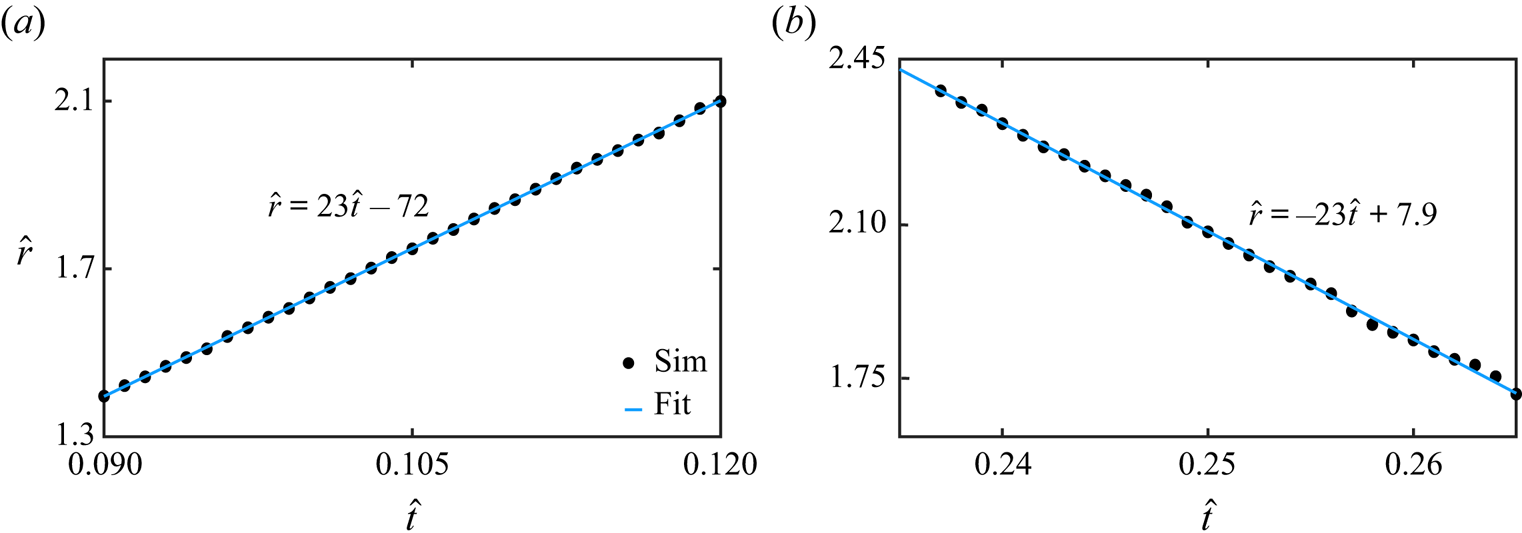
The maximum vertical velocity at the symmetry axis  $v_z^{max}$ for different $Oh$. This figure is a superset of simulation data provided in figure 21(b) with additional data points and power-law fits. The data for $Oh < 1.17\times 10^{-4}$ is indicated as a hashed region to indicate the grid-sensitivity of this data as discussed earlier in Appendix C.
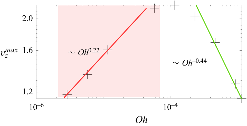


 Open access