


1. Introduction
Irreversible buoyancy flux convergence within oscillating stratified boundary layers on sloping bathymetry in the abyss may be a significant mechanism driving the deep branch of the global overturning circulation (Ferrari et al. Reference Ferrari, Mashayek, McDougall, Nikurashin and Campin2016). The boundary layers, combined with other bottom-intensified sources of turbulence, such as the breaking of internal waves, contribute to observed patterns of intense irreversible buoyancy flux convergence (Polzin Reference Polzin1996) at turbulence ‘hot spots’ (Thorpe Reference Thorpe2007). However, little is known about the laminar, transitional and turbulent processes on gently sloping smooth bathymetry in the ‘tranquil regions’ (Angel Reference Angel1990) of the abyssal ocean. One example of a tranquil region slope is at  $34^{\circ }{\rm N}\ 70^{\circ }{\rm W}$, where the northwest edge of the Sargasso Sea meets the deep end of the continental slope. Modelled maximum (spring tide) tidal current velocities near the seafloor (Turnewitsch et al. Reference Turnewitsch, Falahat, Nycander, Dale, Scott and Furnival2013), assessments of slope criticality (Becker & Sandwell Reference Becker and Sandwell2008) and abyssal mooring observations (Tarbell, Montgomery & Briscoe Reference Tarbell, Montgomery and Briscoe1985; Nash et al. Reference Nash, Kunze, Toole and Schmitt2004) at that location suggest ‘tranquil region’ boundary layers characterized by subcritical slopes, tide velocity amplitudes of less than or approximately equal to $0.01\ {\rm m}\ {\rm s}^{-1}$ and boundary layer thicknesses of ${O}(10)$ m.
How unstable are tranquil region boundary layers on abyssal slopes, and what are the instability mechanisms? In this article, we employ theory and simulations to investigate the pathways between laminar, transitional and turbulent states of boundary layers that are forced by the  $M_2$ barotropic tide and occur on hydraulically smooth abyssal slopes in the absence of forcing by high-wavenumber internal waves, mean flows, far-field turbulence on larger scales and resonant tidal–bathymetric interaction. Although tranquil region abyssal slopes are typically subcritical (Becker & Sandwell Reference Becker and Sandwell2008), we extend our analyses to supercritical slopes for completeness.
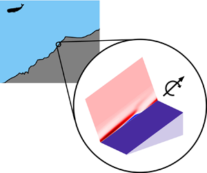
The boundary layers are formed as momentum and buoyancy are diffused by no-slip and adiabatic boundary conditions on sloping bathymetry as low-wavenumber internal waves heave isopycnals (constant-density contours) up and down slopes. Figure 1 illustrates the scale separations between the horizontal length scale of bathymetric features such as continental slopes,  $k^{-1}$, the excursion length scale of the tide, $L$, and the largest boundary layer length scale, $\delta _l$. The excursion length scale, $L$, is the characteristic scale of the across-isobath distance between the trajectory extrema in the inviscid problem, defined as
 \begin{equation} L\sim\frac{U_\infty}{\omega}, \end{equation}
where  $U_\infty$ is the barotropic tide amplitude projected onto the across-slope tangential coordinate ( $x$) and $\omega$ is the tide frequency. We assume that the slope is reasonably approximated as constant on scales of the order of the excursion length, $L$. Thus the boundary layers investigated in this article apply to boundary layer flows on hydraulically smooth slopes where the excursion parameter
 \begin{equation} \mathcal{E}=kL \end{equation}
is small,  $\mathcal {E}\ll 1$. The excursion parameter $\mathcal {E}$ is the ratio of net fluid advection by the barotropic tide to the topographic length. The baroclinic response to the barotropic forcing is highly nonlinear for large-excursion-parameter flows $\mathcal {E}$ (Bell Reference Bell1975a,Reference Bellb; Garrett & Kunze Reference Garrett and Kunze2007; Sarkar & Scotti Reference Sarkar and Scotti2017). Here, we investigate the dynamics on scales at or smaller than the excursion length; thus we assume that the baroclinic tide (or internal waves) generated by bathymetric features with horizontal length scales of $k^{-1}$ can be locally approximated as irrotational over $L\sim {O}(100)$ m. Therefore we model low-wavenumber baroclinic tides, or any oscillatory forcing occurring at frequencies in the range $f<\omega < N$ and characterized by vertical and horizontal structure that can be reasonably approximated as spatially homogeneous over length scales ${O}(10)$ m, as an across-isobath oscillating body force.
Illustration of boundary layers in tranquil abyssal regions at the deep end of a continental slope. The heaving of density surfaces up and down the slope by oscillations with vertical and horizontal structure characterized by length scales much greater than  ${O}(10)$ m creates an oscillating boundary layer.

Non-rotating, large-angle ( $42^{\circ }$), low- $\textit {Re}$ experiments by Hart (Reference Hart1971) showed that, when $\omega ^{2}\ll N^{2}$, ‘plumes’ form during the upward boundary layer flow phase that are mixed and stabilized during the downslope phase. Our objectives are (1) to determine if these boundary layers are laminar, transitional, intermittent or fully turbulent for a range of parameters that include those typical of abyssal ocean non-dimensional parameters associated with the $M_2$ tide, (2) to investigate the transition mechanisms and (3) to test back-of-the-envelope estimation for barotropic tide dissipation rates at the seafloor. The rest of this article is organized as follows. In § 2 we discuss the relevant governing equations and non-dimensional parameters. In § 3 we investigate analytical solutions for the laminar flows to estimate the necessary conditions for boundary layer gravitational instabilities. In § 4 we analyse the stability of simulated boundary layers and in § 5 we summarize the observed transition mechanisms and drag coefficients.
2. Problem formulation
The flows examined in this study are subject to a body force in the across-isobath, or streamwise, direction (the  $x$ direction in figure 1):
 \begin{equation} F_d(t_{d})={-}{\rm Re}[A_{d}\text{ie}^{\text{i}\omega t_{d}}], \end{equation}
where  $A_{d}$ is the dimensional amplitude of the pressure gradient $\partial _x\tilde {P}_{d}$ and $t_{d}$ is dimensional time.
Several geometric and physical approximations are invoked for the sake of tractibility and conceptual simplicity. The flow is approximated as Boussinesq: the density variations are small enough that the incompressibility condition is justified, and Joule heating (increases of internal energy due to the viscous dissipation of mechanical energy) is neglected. We idealize abyssal buoyancy as a linear function of temperature alone.
A Cartesian coordinate system, rotated  $\theta$ radians counterclockwise above the horizontal (figure 1), was chosen for analytical convenience. The $z$ coordinate is the wall-normal (or transverse) coordinate, which is at angle $\theta$ from the vertical coordinate (the coordinate anti-parallel to gravity). To distinguish between the slope-normal and vertical coordinates, the vertical coordinate (and vertical velocities, fluxes, etc.) in the direction normal to Earth's surface will be denoted as $\eta$, such that $\eta =x\sin \theta +z\cos \theta$, shown in figure 1.
The non-dimensional Boussinesq governing equations for conservation of mass, momentum and thermodynamic energy for the flow are
 \begin{gather} \partial_x\tilde{u}+\partial_y\tilde{v}+\partial_z\tilde{w}=0, \end{gather}
 \begin{gather}{d}_t\tilde{{u}}=\frac{1}{{Ro}}\tilde{v}-\partial_x\tilde{p}+ \frac{1}{\textit{Re}_L}\left(\partial_{xx}+\partial_{yy}+\partial_{zz}\right)\tilde{u}+{C}^{2}\tilde{b}+F(t), \end{gather}
 \begin{gather}{d}_t\tilde{{v}}={-}\frac{1}{{Ro}}\tilde{u}-\partial_y\tilde{p}+ \frac{1}{\textit{Re}_L}\left(\partial_{xx}+\partial_{yy}+\partial_{zz}\right)\tilde{v}, \end{gather}
 \begin{gather}{d}_t\tilde{{w}}={-}\partial_z\tilde{p}+ \frac{1}{\textit{Re}_L}\left(\partial_{xx}+\partial_{yy}+\partial_{zz}\right)\tilde{w}+ {C}^{2}\tilde{b}\cot\theta, \end{gather}
 \begin{gather}{d}_t\tilde{{b}}=\frac{1}{\textit{Pr}\,\textit{Re}_L} \left(\partial_{xx}+\partial_{yy}+\partial_{zz}\right)\tilde{b}, \end{gather}
where  ${d}_t=\partial _t+\tilde {\boldsymbol {u}}\boldsymbol {\cdot }\boldsymbol {\nabla }$ and $F(t)=F_{d}(t_{d})/(U_\infty \omega )=A\sin (t)$. The variables are non-dimensionalized as follows (subscript ‘ $d$’ denoting dimensional variables):
 \begin{equation} \boldsymbol{x}={\boldsymbol{x}_{d}}/{L}, \quad \tilde{\boldsymbol{u}}={\tilde{\boldsymbol{u}}_{d}}/{U_{{\infty}}}, \quad t={\omega}{t_{d}}, \quad \tilde{p}={\tilde{p}_{d}}/{U_{{\infty}}^{2}}, \quad \tilde{b}={\tilde{b}_{d}}/{(LN^{2}\sin\theta)}, \end{equation}
where the reference density  $\rho _0$ is absorbed into the mechanical pressure $p_{d}$ such that it has units of ${\rm J}\ {\rm kg}^{-1}$. Parameter $N^{2}$ is the square of the buoyancy frequency (the natural frequency associated with the restoring force of stratification). The buoyancy is defined as the acceleration associated with density anomalies, $b_{d}=g(\rho _0-\rho )/\rho _0$, where $g$ is the (constant) gravity and $\rho$ is the density.
Despite the assumptions and idealizations listed above, the dynamical parameter space is vast. The relevant non-dimensional ratios are the Prandtl number  $\textit {Pr}$, the slope Rossby number ${Ro}$, the slope frequency ratio ${C}$ and Stokes layer Reynolds number $\textit {Re}$. In this study, the Stokes layer Reynolds number is referred to in the analysis of the flow instead of the excursion length Reynolds number,
 \begin{equation} \textit{Re}_L=\frac{U_\infty L}{\nu}=\frac{U_\infty^{2}}{\nu\omega}, \end{equation}
because the Stokes layer Reynolds number is common in literature regarding oscillating boundary layers. The Prandtl and Stokes layer Reynolds numbers are defined as
 \begin{gather} \textit{Pr}=\frac{\nu}{\kappa}, \end{gather}
 \begin{gather}\textit{Re}=\frac{U_\infty\delta}{\nu}=\sqrt{2\textit{Re}_L}, \end{gather}
where  $\kappa$ is the molecular diffusivity of buoyancy and $\nu$ is the kinematic viscosity of abyssal seawater, and where the Stokes layer thickness is
 \begin{equation} \delta=\sqrt{2\nu/\omega}. \end{equation}
The slope frequency ratio is defined as the ratio of the projection of the buoyant acceleration onto the across-slope ( $x$) direction (parallel to the forcing) to the acceleration of the oscillatory forcing:
 \begin{equation} {C}=\frac{N\sin\theta}{\omega}. \end{equation}
The slope frequency ratio was first identified as an important ratio for describing the boundary layer by Hart (Reference Hart1971) (who denoted it as  ${Q}$, where ${Q}={C}^{2}$), while the frequency ratio $N/\omega$ emerges as an important measure of the role of stratification in the stratified form of Stokes’ second problem (Gayen & Sarkar Reference Gayen and Sarkar2010a). The slope frequency ratio is indicative of the degree of resonance between the oscillation body forcing and the buoyant restoring force.
Finally, the fourth non-dimensional ratio is the slope Rossby number:
 \begin{equation} {Ro}=\frac{\omega}{f\cos\theta}, \end{equation}
which indicates the ratio of the influence of planetary vorticity (projected onto the wall-normal direction) relative to vorticity with a characteristic time scale of the tide period,  $\omega ^{-1}$. For the finite-Rossby-number cases examined, $\omega$ is the $M_2$ tide frequency, the Coriolis parameter, $f$, is $10^{-4}\ {\rm s}^{-1}$ and the range of slope angles investigated are within $0<\theta \leqslant 14^{\circ }$. Therefore, the slope Rossby number is approximately 1.4 for all of the rotating reference frame flows investigated.
2.1. Inviscid, linear flow
The inviscid, linearized forms of the governing equations (2.2)–(2.6) describe the heaving of isopycnals up and down the slope:
 \begin{gather} \partial_t\tilde{{u}}=\frac{1}{{Ro}}\tilde{v}+{C}^{2}\tilde{b}+F(t), \end{gather}
 \begin{gather}\partial_t\tilde{{v}}={-}\frac{1}{{Ro}}\tilde{u}, \end{gather}
 \begin{gather}\partial_t\tilde{{b}}={-}\tilde{{u}}. \end{gather}
Crucially, the solutions to (2.14)–(2.16) prescribe the amplitude of the non-dimensional body force:
 \begin{equation} A=\left({C}^{2}+\frac{1}{{Ro}^{2}}-1\right),\end{equation}
where  $A_{d}=AU_\infty \omega$. The solutions to (2.16)–(2.16) are
 \begin{gather} \tilde{{u}}(t)={-}\cos(t), \end{gather}
 \begin{gather}\tilde{{v}}(t)={Ro}^{{-}1}\sin(t), \end{gather}
 \begin{gather}\tilde{{b}}(t)=\sin(t). \end{gather}
2.2. Resonance
The assumption that the vertical and horizontal structure of an internal wave is constant over a length scale of  ${O}(10)$ m is not valid if the wave is critical. At critical slope, the forcing model $F(t)$ in (2.1) and (2.14) is degenerate and vanishes if the critical slope condition
 \begin{equation} {C}^{2}+\frac{1}{{Ro}^{2}}-1=0 \end{equation}
is satisfied. If (2.21) is satisfied, the energy of the inviscid baroclinic tide is tightly focused into narrow beams that follow the curvature of the bathymetry (Balmforth, Ierley & Young Reference Balmforth, Ierley and Young2002).
Equation (2.21) is formally consistent with internal wave theory. In internal wave theory, critical slopes are defined by
 \begin{equation} \tan\theta_c=\sqrt{\frac{\omega^{2}-f^{2}}{N^{2}-\omega^{2}}}, \end{equation}
where  $\theta _c$ is the critical slope angle. If the slope angle $\theta \neq \theta _c$, then (2.17) is satisfied, $A\neq 0$. Equation (2.17) can be rearranged to obtain
 \begin{equation} \tan\theta=\sqrt{\frac{\omega^{2}(1+A)-f^{2}}{N^{2}-\omega^{2}(1+A)}}. \end{equation}
Therefore the criticality condition in (2.21) is just a rearrangement of the criticality condition defined by the slope parameter  $\epsilon$ from internal wave theory:
 \begin{equation} \epsilon=\frac{\tan\theta}{\tan\theta_c}, \end{equation}
where criticality states are defined:
 \begin{equation} \left.\begin{array}{llllll@{}} \text{if} & A<0 & \text{then} & \epsilon<1 & \rightarrow & \theta\ \text{is subcritical},\\ \text{if} & A=0 & \text{then} & \epsilon=1 & \rightarrow & \theta\ \text{is critical},\\ \text{if} & A>0 & \text{then} & \epsilon>1 & \rightarrow & \theta\ \text{is supercritical}. \end{array}\right\} \end{equation}
2.3. Boundary conditions
At the solid boundary at  $z=0$, the boundary conditions on the total velocity are no-slip and impermeability
 \begin{equation} \tilde{\boldsymbol{u}}=0, \end{equation}
and the boundary conditions on the total buoyancy is the adiabatic condition:
 \begin{equation} \partial_z\tilde{b}=0. \end{equation}
As  $z\rightarrow \infty$, the velocity boundary conditions are the oscillatory solutions for the inviscid flow, and zero flow in the wall-normal direction: (2.18), (2.19) and $\widetilde {{w}}=0$. The non-dimensional buoyancy field as $z\rightarrow \infty$ has two components, the inviscid oscillation and the constant background stratification:
 \begin{equation} \tilde{{b}}=x+z\cot\theta+\sin(t). \end{equation}
2.4. Variable decomposition
The total velocity and buoyancy fields are decomposed into three components that when summed together satisfy (2.2)–(2.6) and (2.26)–(2.28). To distinguish the components, let ‘ $H$’ denote the hydrostatic (and possibly geostrophic) component, let ‘ $S$’ denote the steady component and let ‘ $O$’ denote the oscillating component:
 \begin{gather} \tilde{\boldsymbol{u}}(x,y,z,t)= \boldsymbol{u}_{{H}}+\boldsymbol{u}_{{S}}(z)+\boldsymbol{u}_{{O}}(x,y,z,t), \end{gather}
 \begin{gather}\tilde{b}(x,y,z,t)=b_{{H}}(x,z)+b_{{S}}(z)+b_{{O}}(x,y,z,t), \end{gather}
 \begin{gather}\tilde{p}(x,y,z,t)=p_{{H}}(x,z)+p_{{S}}(z)+p_{{O}}(x,y,z,t). \end{gather}
The hydrostatic component of the buoyancy field is merely the background stratification in the rotated coordinate system,  $b_{{H,d}}(x_{d},z_{d}) =N^{2}(x_{d}\sin \theta +z_{d}\cos \theta )$ in dimensional form, and the quiescent hydrostatic velocity field $\boldsymbol {u}_{{H}}=0$ everywhere except in the finite-Rossby-number flow regime, in which case it is the along-slope geostrophic velocity that arises from the across-isobath pressure gradient imposed by the slope (Phillips Reference Phillips1970; Wunsch Reference Wunsch1970). The buoyancy frequency $N$ is defined in the same manner as convention:
 \begin{equation} N^{2}={-}\frac{g}{\rho_0}\partial_\eta{\rho}_{{H}}=\partial_\eta{b}_{{H,d}}, \end{equation}
where  $\eta$ denotes the vertical position coordinate as shown in figure 1.
The steady and oscillating flow components are anomalies from the hydrostatic background that ensure the satisfaction of frictional and diffusive boundary conditions at the wall and inviscid oscillations far from the wall. It is convenient to solve for the anomalies,
 \begin{gather} \boldsymbol{u}(x,y,z,t)=\boldsymbol{u}_{{S}}(z)+\boldsymbol{u}_{{O}}(x,y,z,t), \end{gather}
 \begin{gather}b(x,y,z,t)=b_{{S}}(z)+b_{{O}}(x,y,z,t), \end{gather}
 \begin{gather}p(x,y,z,t)=p_{{S}}(z)+p_{{O}}(x,y,z,t), \end{gather}
because the removal of the hydrostatic background permits periodic analytical and numerical solutions for  $\boldsymbol {u}$ and $b$.
$b$.
3. Linear solutions
Analytical solutions to linearized forms of (2.2)–(2.6) contain a wealth of information pertaining to the laminar, disturbed laminar and intermittently turbulent regimes (i.e. low- to moderate-Reynolds-number flows) that are investigated numerically in this study. Thorpe (Reference Thorpe1987) provided solutions of the rotating linear problem, a detailed derivation of which is given in Appendix A. The solutions in Appendix A are written in a form that readily collapses in the  ${Ro}\rightarrow \infty$ regime.
3.1. Necessary conditions for gravitational instability
The linear solutions for the steady flow component of both rotating and non-rotating flows is always gravitationally stable, meaning that the total vertical buoyancy gradient is never negative,
 \begin{equation} \partial_{\eta}b_{H}+\partial_{\eta}b_{S} =1-\cos^{2}\theta\mathrm{e}^{-\eta/\delta_{S}} \sqrt{2}\sin\left(\frac{\eta}{\delta_{S}}+\frac{\rm \pi}{4}\right)\geqslant 0, \end{equation}
if the oscillating component vanishes. The boundary layer thickness of the steady component (Phillips Reference Phillips1970; Wunsch Reference Wunsch1970) is
 \begin{equation} \delta_{S}=\left(\frac{f^{2}\cos^{2}\theta}{4\nu^{2}} +\textit{Pr} \frac{N^{2}\sin^{2}\theta}{4\nu^{2}}\right)^{{-}1/4}. \end{equation}
The oscillating flow component solutions exhibit transient gravitationally unstable buoyancy gradients,  $\delta _\eta \tilde {b}<0$, when denser fluid is advected over lighter fluid during portions of the oscillation period. If the oscillating component is non-zero, then the minimum necessary condition for gravitational instabilities is defined by
 \begin{equation} \partial_{\eta}b_{H}+\partial_{\eta}b_{S}<{-}\partial_{\eta}b_{O}, \end{equation}
because if (3.3) is satisfied, then the total vertical buoyancy gradient is negative,  $\delta _\eta \tilde {b}<0$. However, instabilities can grow only if the negative buoyancy gradient is sustained for a significant amount of time and if it is negative enough to overcome resistance from friction.
A characteristic boundary layer Rayleigh number and a ratio of the time scale of the growth of an instability to the period of the oscillation are required to estimate the minimum (quasi-steady) conditions for the growth of gravitational instabilities. However, the linear solutions do not readily yield a single boundary layer buoyancy gradient length scale. If the buoyancy gradient length scale is assumed to scale with  $\delta =\sqrt {2\nu /\omega }$, then a tenable time-dependent boundary layer Rayleigh number is defined:
 \begin{equation} {Ra}(t)\sim\frac{4\textit{Pr} N^{2}}{\omega^{2}}\partial_\eta\tilde{b}(t), \end{equation}
which only applies when  $\partial _\eta \tilde {b}(t)<0$. To estimate the gravitational stability of the flow without explicitly accounting for the time dependence of the basic state (the quasi-steady assumption), the basic state of the flow cannot change more rapidly than the growth rate of a gravitational instability. If the instabilities are ‘slowly modulated’ by the basic state (Davis Reference Davis1976), the quasi-steady assumption is reasonable for stability analysis. The dimensional instantaneous growth rate of a gravitational instability can be estimated as
 \begin{equation} \sigma\sim{\rm Im}\left[\sqrt{\partial_\eta \tilde{b}N^{2}}\right]. \end{equation}
If  $|{\omega }/{\sigma }|\ll 1$, then the modulation by the basic state is sufficiently slow for the growth of gravitational instabilities.
Figure 2 shows the minimum values of the non-dimensional total vertical buoyancy gradient from the linear solutions for non-rotating and rotating cases as a function of slope parameter and Stokes Reynolds number. Assuming that the gravitational instability in the boundary layer is physically similar to that of Rayleigh–Bénard instability in the case of one rigid and one stress-free boundary, then the critical Rayleigh number for the boundary layer is  ${Ra}_c\approx 1100$ (Chandrasekhar Reference Chandrasekhar1961), which corresponds to $|\omega /\sigma |=0.06$. For the chosen fluid properties (holding $\textit {Pr}=1$, $f=10^{-4}$, $N=10^{-3}$ and ${\omega =1.4\times 10^{-4}}$ constant), ${Ra}_c\approx 1100$ corresponds to a critical non-dimensional vertical buoyancy gradient of $\partial _\eta \tilde {b}=-5.4$, which is shown as the blue lines in figure 2. The minimum boundary layer buoyancy gradient is less than zero for all non-zero $\textit {Re}$ and $\epsilon$, and the minimum boundary layer buoyancy gradient is increasingly negative with increasing Reynolds number and with increasing slope parameter. The discontinuity at $\epsilon =1$ is an artefact of the degeneracy of linear solutions at critical slope. The $\epsilon$ axis between the non-rotating and rotating cases is different because rotation alters the angle of critical slope; both plots show the same slope angle range, $0<\theta \leqslant 16^{\circ }$.
Total buoyancy gradient minima. The minimum value (in both time and space) of the non-dimensional linear solution vertical buoyancy gradient for (a) the non-rotating reference frame case ( $f=0$) and (b) the rotating reference frame case.

4. Nonlinear solutions
In this section we examine the nonlinear stability and development of turbulence in boundary layers on smooth abyssal slopes for both rotating and non-rotating regimes. The boundary layers are initialized by the oscillating laminar flow solutions derived in Appendix A. We varied the slope Rossby number (nearly constant with slope, (2.13)), slope frequency ratio (2.12), Reynolds number (2.10), slope parameter (2.24) and slope angle  $\theta$ for each of the 16 simulations as shown in table 1. The slope frequency ratio ${C}$ and slope parameter $\epsilon$ are redundant for the non-rotating case, but are shown together because ${C}\neq \epsilon$ for the rotating flow, and ${C}$ appears explicitly in the forcing of the across-isobath ( $x$) momentum equation. We observed bursts of turbulence, triggered by two-dimensional gravitational instabilities that rapidly become three-dimensional, during the upslope flow phase of all cases at $\textit {Re}=840$ except for the case of lowest slope Burger number, which exhibits turbulence sustained throughout the period. At $\textit {Re}=420$, the flow matched the laminar analytical solutions except for weak turbulent bursts that occurred at the highest slope angles in the rotating regime.
Prescribed non-dimensional simulation parameters. The four independent parameters are  $\textit {Re}$, ${Ro}$, ${C}$, $\theta$, where $\textit {Pr}=1$ is not varied. The slope parameter $\epsilon =\tan \theta /\tan \theta _c$ is also used in this study to directly connect results to internal wave parameters. The slope Burger number is ${Bu}={N^{2}\tan ^{2}\theta }/f^{2}={Ro}^{2}{C}^{2}$.

4.1. Numerical implementation
The flow anomalies, as defined by (2.33) and (2.34), are discretized to satisfy periodic boundary conditions in the wall-parallel directions via Fourier spectral bases in the across-isobath ( $x$) and along-isobath ( $y$) directions. Periodicity is not merely numerically convenient; it also eliminates the need to prescribe buoyancy forcing (‘restratification’) because the oscillating flow can advect the background field to gain or lose buoyancy. In the periodic domain, the boundary layer buoyancy can only reach a homogenized steady state if the turbulence sustainably converts tidal momentum to potential energy throughout the entire period.
Although the planar extent of the computational domain is less than the excursion length of the tide, the domain size (table 2) is justifiably sufficient because the largest eddies in oscillating boundary layers are those associated with the transverse (wall-normal) length scale, which is much less than the excursion length. Indeed, at higher Reynolds number ( $\textit {Re}=1790$), Gayen & Sarkar (Reference Gayen and Sarkar2010b) found the turbulent boundary layer thickness, $\delta _l$, was $\delta _l=15\delta$ for the unstratified problem and $\delta _l=17\delta$ for flat-plate stratified oscillating boundary layers at the same Reynolds number. The grid resolution parameters for the two Reynolds numbers examined are shown in table 2, where ( $L_x,L_y,H$) are the domain dimensions in ( $x,y,z$), $l_{K}$ and $\tau _{K}$ are the Kolmogorov length and time scales, respectively, and wall units (denoted by superscript $+$) are scaled by the viscous length scale $\delta _v=\nu /U_*$, where $U_*$ is the a priori estimate of the friction velocity, which is approximated as $U_*=\sqrt {\nu \partial _z\bar {u}}\sim \sqrt {\nu {U_\infty }/{\delta }}$.
Resolution parameters. The grid is identical in the  $x$ and $y$ directions. Kolmogorov scales are estimated assuming that the law of the wall holds; therefore, characteristic dissipation rate is estimated a priori by $\varepsilon \sim U_*^{3}/(\delta \kappa _*)$, where the von Kármán constant is $\kappa _*=0.41$ and the friction velocity is estimated by $U_*\sim \sqrt {\nu U_\infty /\delta }$.

Our decomposition of the flow is the same as that of Phillips (Reference Phillips1970) and Wunsch (Reference Wunsch1970): we decompose the flow into a quiescent, hydrostatic background flow (denoted by the subscript ‘ $H$’ variables in (2.29), (2.30) and (2.31), where $\boldsymbol {u}_{H}=0$) and solve for anomalies from the background flow (the left-hand sides of (2.33), (2.34) and (2.35)) that, when summed with the background flow component, satisfy the no-slip (2.26) and adiabatic (2.27) boundary conditions at the wall imposed on the total flow. The nonlinear governing equations for the anomalies are
 \begin{gather} \partial_x{u}+\partial_y{v}+\partial_z{w}=0, \end{gather}
 \begin{gather}{d}_t{{u}}=\frac{1}{{Ro}}{v}-\partial_x{p}+ \frac{1}{\textit{Re}_L}\left(\partial_{xx}+\partial_{yy}+ \partial_{zz}\right){u}+{C}^{2}{b}+F(t), \end{gather}
 \begin{gather}{d}_t{{v}}={-}\frac{1}{{Ro}}{u}-\partial_y{p}+ \frac{1}{\textit{Re}_L}\left(\partial_{xx}+\partial_{yy}+\partial_{zz}\right){v}, \end{gather}
 \begin{gather}{d}_t{{w}}={-}\partial_z{p}+ \frac{1}{\textit{Re}_L}\left(\partial_{xx}+\partial_{yy}+\partial_{zz}\right){w} +{C}^{2}{b}\cot\theta, \end{gather}
 \begin{gather}{d}_t{{b}}=\frac{1}{\textit{Pr} \,\textit{Re}_L} \left(\partial_{xx}+\partial_{yy}+\partial_{zz}\right){b}, \end{gather}
where the anomalies  ${u},v,w,p$ and $b$ are defined by (2.33)–(2.35). The material derivative on the left-hand side of (4.5) contains nonlinear buoyancy anomaly advection terms as well as the terms describing the time rate of change of anomalous buoyancy, $-(u+w\cot \theta )$, by the advection of background buoyancy. Since the linear solutions for the oscillating laminar flow (Thorpe Reference Thorpe1987; Baidulov Reference Baidulov2010) contain only the advective terms corresponding to the background buoyancy advection, the laminar stratification oscillates from negative to positive and back again in a linear advection–diffusion balance. However, the boundary layer stratification can weaken, relative to the oscillating laminar stratification, if the vertical gradient of the nonlinear anomalous buoyancy advection in (4.5) is negative and dominates the vertical gradient of background buoyancy advection. Therefore, gradients of nonlinear anomalous buoyancy advection must continually overcome the restratifying tendency of background buoyancy advection (e.g. $u>0$ corresponds to a local decrease in buoyancy as relatively heavy fluid is advected upslope) for weakened boundary layer stratification to persist.
The anomalies were computed using the MPI-parallel pseudo-spectral partial differential equation solver Dedalus (Burns et al. Reference Burns, Vasil, Oishi, Lecoanet and Brown2019) using  $128^{3}$ modes. A third-order, four-stage, implicit–explicit Runge–Kutta method derived by Ascher, Ruuth & Spiteri (Reference Ascher, Ruuth and Spiteri1997) was used for temporal integration. Chebyshev polynomial bases of the first kind were employed for spatial discretization on a cosine grid in the wall-normal direction. Chebyshev polynomials permit the exact enforcement of the adiabatic wall-boundary condition ((2.27) minus the background component) on the buoyancy field and no-slip/impermeability wall-boundary conditions on the velocities ((2.26) minus the background component). The $3/2$ rule dealiasing scheme is used not only for dealiasing the spatial modes online but also for dealiasing post-processed flow statistics.
At the maximum wall-normal extent of the domain, the boundary conditions at infinity (2.18), (2.19) and (2.28) were approximated for the anomalies as free-slip, impermeable conditions:
 \begin{equation} \partial_zu=\partial_zv=w=0, \end{equation}
and an adiabatic condition on just the anomaly:
 \begin{equation} \partial_zb=0, \end{equation}
such that the total flow buoyancy gradient at  $z=H$ is the background buoyancy gradient in that direction.
Although the impermeability condition causes the reflection of internal waves that reach the upper boundary, the effects are assumed to be negligible because of the negligible amount of energy propagated by such high-wavenumber waves in low-Reynolds-number flow. Gayen & Sarkar (Reference Gayen and Sarkar2010a) found that for flat-bottomed stratified oscillatory flow at larger-Reynolds-number flow ( $\textit {Re}=1790$), the vertical wave energy flux is less than 1 % of the boundary layer dissipation and production rates. Indeed, small but non-zero dissipation rates of turbulent kinetic energy (TKE) were found near the upper boundary in some of the simulations, presumably from subharmonic parametric instability or other wave–wave instabilities because of the free-slip reflective upper boundary condition. However, 99.9 % of the shear production rate and dissipation rate occurred within one Ozmidov length of the wall ( $L_O=\sqrt {\varepsilon /N^{3}}$, using the magnitude of the background stratification for $N$) at the lower boundary for all simulations.
A small amount of grid-scale noise was observed primarily in the  $x,y$ directions for $\textit {Re}=840$ cases. However, the wall-normal integrated TKE balances (figure 4) the residual of the right-hand-side TKE equation terms and the calculation of $\partial _tK$ matched to graphical accuracy, suggesting the grid-scale noise did not significantly alter energetics. The resolution of $\Delta x/l_K=\Delta y/l_K=13.8,18.0$ (table 2) was chosen by estimating the characteristic scale of $\varepsilon ={O}(10^{-10}) \ \textrm {m}^{2}\ \textrm {s}^{-3}$ a priori assuming fully developed steady turbulence that satisfies the law of the wall, even though law-of-the-wall turbulence was not anticipated because of the transitional Reynolds numbers prescribed. The a priori estimate $\varepsilon ={O}(10^{-10})\ \textrm {m}^{2}\ \textrm {s}^{-3}$ roughly agrees with the majority of the corresponding a posteriori average dissipation rates shown in table 4, despite the false assumptions of the a priori estimate. Since the TKE equation closes to graphical accuracy and the instabilities investigated are laminar in origin, we anticipate that the results of this study will remain the same at higher resolution. However, the small amount of signal attenuation at the Nyquist wavenumbers suggests that the shear production and dissipation rates may be slightly underestimated.
The initial conditions were specified as the sum of the steady component (Phillips Reference Phillips1970; Wunsch Reference Wunsch1970), the oscillating component (Thorpe Reference Thorpe1987) at time  $t=0$ and uniformly distributed white noise corresponding to buoyancy anomaly perturbations of magnitude $10^{-10}\ \textrm {m}\ \textrm {s}^{-2}$. All of the simulations that exhibited turbulence (defined as wall-normal integrated production rates of TKE greater than $10^{-10}\ \textrm {m}^{3}\ \textrm {s}^{-3}$) did so within two oscillations.
The parameter regimes shown in table 1 qualitatively describe flows forced by the  $M_2$ tide frequency, which is specified as $\omega =1.4\times 10^{-4}$ ( $\textrm {rad}\ \textrm {s}^{-1}$, for a 12.4 h tide period) and the Coriolis parameter is specified as $f=10^{-4}$ ( $\textrm {rad}\ \textrm {s}^{-1}$). Much of the abyssal ocean is filled with Antarctic Bottom Water (AABW), characterized by temperatures near $0\,^{\circ }\textrm {C}$ and practical salinities of approximately 35 psu. At $0\,^{\circ }\textrm {C}$ and 35 psu, the kinematic viscosity is $1.8\times 10^{-6}\ \textrm {m}^{2} \ \textrm {s}^{-1}$ (Chen et al. Reference Chen, Chan, Read and Bromley1973; Talley Reference Talley2011) and the thermal diffusivity is $1.4\times 10^{-7}\ \textrm {m}^{2}\ \textrm {s}^{-1}$ (Thorpe Reference Thorpe2007); thus $Pr\approx 13$ for AABW. We specify the kinematic viscosity as $\nu =2\times 10^{-6}\ \textrm {m}^{2}\ \textrm {s}^{-1}$ in the relevant parameters in table 1 and $Pr=1$ for simplicity. We approximate the background buoyancy frequency at mid-latitude abyssal depths as $N=10^{-3}\ \textrm {rad}\ \textrm {s}^{-1}$ (Thurnherr & Speer Reference Thurnherr and Speer2003). Baroclinic tide amplitudes of $U_{\infty }\leqslant 0.01\ \textrm {m}\ \textrm {s}^{-1}$ in tidal models (Turnewitsch et al. Reference Turnewitsch, Falahat, Nycander, Dale, Scott and Furnival2013) agree with observations at the northwestern edge of the Sargasso Sea at $34^{\circ }\textrm {N}\ 70^{\circ }\textrm {W}$ (Tarbell et al. Reference Tarbell, Montgomery and Briscoe1985; Nash et al. Reference Nash, Kunze, Toole and Schmitt2004). Global assessments of slope criticality suggest that the same region is characterized by subcritical, low-angle slopes. We also examine supercritical slopes for completeness. The prescribed non-dimensional parameters in table 1 were varied by only varying the velocity, $U_\infty =0.01,0.005\ \textrm {m}\ \textrm {s}^{-1}$ corresponding to the two Reynolds numbers, and the slope angle (shown in the rightmost column of table 1).
4.2. Intermittent turbulent bursts
The integrated TKE budget of each simulation was computed in order to distinguish the laminar and turbulent regimes and to quantify turbulence production mechanisms. The planar mean TKE is defined as
 \begin{equation} K(z,t)\equiv\tfrac{1}{2}\left(\overline{u'^{2}}+\overline{v'^{2}}+\overline{w'^{2}}\right), \end{equation}
where the planar mean operator and variable decomposition are defined:
 \begin{gather} \bar{\phi}(z,t)=\frac{1}{L_xL_y}\int_{{-}L_x/2}^{L_x/2}\int_{{-}L_y/2}^{L_y/2} \phi(y,z,t)\,{\rm d} y\,{\rm d}x, \end{gather}
 \begin{gather}\phi(x,y,z,t)=\bar{\phi}(z,t)+\phi'(x,y,z,t), \end{gather}
and  $\phi$ is any of the anomalous variables defined by (2.33)–(2.35). The planar mean TKE evolution equation is
 \begin{equation} {\partial_t{K}} +\partial_{z}\mathcal{T} =\mathcal{P} +\mathcal{B} -\varepsilon. \end{equation}
The TKE transport term  $\partial _{z}\mathcal {T}$ includes all TKE flux divergences (mean, turbulent, pressure, diffusion), which vanish upon wall-normal integration of (4.11). The rate production of TKE by mean shear is $\mathcal {P}$ (production in the sense that, generally, $\mathcal {P}>0$), and it is defined as
 \begin{gather} \mathcal{P}(z,t)={-}\overline{u'w'}\partial_z\bar{u}-\overline{v'w'}\partial_z\bar{v}, \end{gather}
 \begin{gather}\mathcal{P}_{13}={-}\overline{u'w'}\partial_z\bar{u}, \end{gather}
 \begin{gather}\mathcal{P}_{23}={-}\overline{v'w'}\partial_z\bar{v}. \end{gather}
The buoyancy flux  $\mathcal {B}$ is typically downgradient ( $\mathcal {B}<0$ amidst $\partial _z\bar {b}>0$ or $\mathcal {B}>0$ amidst $\partial _z\bar {b}<0$), in which case it represents the conversion of TKE into potential energy, and it is defined as
 \begin{gather} \mathcal{B}(z,t)=\overline{w_\eta'b'}=\overline{u'b'}\sin\theta+\overline{w'b'}\cos\theta, \end{gather}
 \begin{gather}\mathcal{B}_1=\overline{u'b'}\sin\theta, \end{gather}
 \begin{gather}\mathcal{B}_3=\overline{w'b'}\cos\theta \end{gather}
in the rotated reference frame (where  $w_\eta ={d}_t\eta$ is the velocity in the vertical, not the wall-normal velocity $w$). Defined in this manner a downgradient buoyancy flux may be reversible. A reversible buoyancy flux may be thought of as a buoyancy flux that converts TKE into potential energy through stirring alone. Finally, the dissipation rate of TKE
 \begin{align} \varepsilon(z,t)&=\nu\left( \overline{(\partial_x{u'})^{2}} +\overline{(\partial_x{v'})^{2}} +\overline{(\partial_x{w'})^{2}} +\overline{(\partial_y{u'})^{2}} +\overline{(\partial_y{v'})^{2}}\right. \nonumber\\ &\quad \left.+\overline{(\partial_y{w'})^{2}} +\overline{(\partial_z{u'})^{2}} +\overline{(\partial_z{v'})^{2}} +\overline{(\partial_z{w'})^{2}}\right) \end{align}
is positive definite and therefore the last term of (4.11) is always a sink of TKE.
The laminar oscillating boundary layer buoyancy gradient is transient and evanescent; therefore, we seek an integral quantity to measure the stabilizing/destabilizing effects of the time-periodic laminar buoyancy gradient. We borrow the concept of boundary layer displacement thickness (Monin & Yaglom Reference Monin and Yaglom1971) and apply it to transient bulk buoyancy gradients rather than momentum. We refer to this measure as the boundary layer stratification thickness,  $\delta _s$. If the total buoyancy field is not constant over small distance in the wall-normal direction $z_1$, then it can be approximated as constant over some distance $z_0$ from the wall, where $z_0$ is defined by
 \begin{equation} N^{2}z_0=\int_0^{z_1}\partial_z\tilde{b}\,\mathrm{d}z. \end{equation}
It follows that
 \begin{equation} \delta_s=z_1-z_0=\int_0^{z_1}\left(1-\frac{\partial_z\tilde{b}}{N^{2}}\right)\mathrm{d}z. \end{equation}
Since  $\partial _z\tilde {b}\rightarrow N^{2}$ as $z_1\rightarrow \infty$ the integrand of (4.20) vanishes as $z_1\rightarrow \infty$.
Figure 3 shows the geometric interpretation of (4.19). Here  $\delta _s>0$ and indicates that, in bulk, the oscillating laminar boundary layer stratification is less than the background stratification, and vice versa as the sign of the laminar boundary layer buoyancy gradient oscillates from negative to positive in the laminar flow solutions provided in Appendix A. The stratification thickness is positive when heavier fluid is advected over lighter fluid that has been impeded from flowing upslope by molecular friction at the boundary. Note that $\delta _s<0$ for the laminar steady flow component solutions because the analytical solutions (Phillips Reference Phillips1970; Wunsch Reference Wunsch1970) require steady positive bulk stratification near the boundary, where isopycnals curve downwards. The stratification thickness was calculated for each flow investigated here, using the linear analytical solutions for the laminar oscillating flows and setting $z_1\gg 1$.
(a–d) Stratification thickness concept.

The wave- and planar-averaged, wall-normal integrated TKE budget statistics for  $\textit {Re}=840$ are shown in figure 4. The statistics were wave-averaged over 5–10 oscillations. All of the integrated TKE budgets at $\textit {Re}=840$, with the exceptions of case 5 and arguably case 7, possess a single burst of chaotic three-dimensional motion that is characterized by a rapid increase in the production rate of the TKE from the across-slope shear, $\mathcal {P}_{13}$, the component of shear parallel to the direction of the oscillating body force. The turbulent bursts, which occur shortly after $t/T\approx 0.5$, preferentially select the phase regime during which the velocity is upslope but decelerating, the sign of the oscillating buoyancy changes from positive to negative and the stratification thickness is negative (as indicated by the dark grey shading in figure 4). The negative stratification thickness preference of the bursts contrasts the low-Reynolds-number, intermittent turbulence regime of Stokes’ second problem, in which a single burst occurs per oscillation, corresponding to the random selection of one of two shear maxima that occur within one period (Spalart & Baldwin Reference Spalart and Baldwin1987).
(a–h) Wall-normal integrated, planar mean TKE budgets. The grey shading corresponds to the sign of the stratification thickness (negative (positive) represents enhanced (weak or negative) bulk boundary layer stratification). The dashed lines correspond to the time of the minimum total vertical buoyancy gradient in the linear solutions. The far-field velocity oscillates with  $-\cos (t)$.

To investigate the role of the linear buoyancy dynamics in the formation of the turbulent bursts in figure 4, the time of the minimum total vertical buoyancy gradient in the linear solutions, which the reader may recall is negative for all of the considered parameter space as shown in figure 2, is depicted as the vertical dashed black line. The maximum TKE production rate by the mean shear approximately coincides in the time of the minimum total vertical buoyancy gradient for cases 1 and 6, the smallest intensity turbulent bursts shown in figure 4. The shear production is predominantly by  $\mathcal {P}_{13}$, consistent with the notion that $w'>0$ disturbances initiated by gravitational instabilities impede the mean shear and trigger $u'<0$. The negative Reynolds stresses combined with $\partial _z\bar {u}>0$ during the upslope flow at $t\approx 0.5$ subsequently produce $\mathcal {P}_{13}>0$ as plotted in figure 4. In the rotating cases, $\mathcal {P}_{23}$ is non-zero as mean shear in the along-isobath direction provides a source of TKE which is present in the non-rotating regime. This result suggests that the bursts of TKE production rate by the mean shear are triggered by buoyant ejections of low-momentum fluid upward. However, the triggering of buoyancy ejections is brief, weak and not sustained, because the buoyancy fluxes in figure 4 are negligible prior to bursts in the along-isobath shear production. Thus the gravitational instabilities appear to initiate, but not drive, bursts of chaotic three-dimensional motion.
It is well known that boundary layer turbulence is inherently anisotropic. However, the majority of ocean turbulence measurements measure the fluctuations of the vertical shear of the horizontal velocities and then assume homogeneous isotropic turbulent motion to subsequently estimate the dissipation rate (Polzin & Montgomery Reference Polzin and Montgomery1996; St. Laurent, Toole & Schmitt Reference St. Laurent, Toole and Schmitt2001). The isotropic, homogeneous turbulence dissipation rate of TKE (Taylor Reference Taylor1935) is defined in the sloped coordinate frame as
 \begin{equation} \varepsilon_{hi}= \tfrac{15}{4}\nu\cos^{2}\theta\left(\overline{(\partial_zu')^{2}} +\overline{(\partial_zv')^{2}}\right). \end{equation}
The wall-normal integrated forms of  $\varepsilon _{hi}$ are plotted for the rotating reference frame cases in figure 4. Comparison of the dissipation rate assuming homogeneous isotropic turbulence (4.21) and the full dissipation rate (4.18), shown for the rotating cases, indicates that the assumption of homogeneous isotropic turbulence leads to overpredictions of the dissipation rate by a factor of approximately two. At high Reynolds number in unstratified boundary layers it is well known that the boundary layer dissipation rate is highly anisotropic in the viscous sublayer (Pope Reference Pope2000); therefore we speculate that, if the Prandtl number remains unity, then the anisotropy of the dissipation rate will be similarly significant in the viscous sublayer of the high-Reynolds-number regimes of the flow investigated here.
4.3. Gravitationally unstable rolls
Except for case 6, all of the simulations at  $\textit {Re}=840$ exhibited rolls characterized by growing streamwise vorticity. Figure 5 shows the instantaneous vertical velocity of case 2 to illustrate the life cycle of the rolls. In figure 5, red corresponds to upward motions and blue approximately corresponds to downward motions. The generation of two-dimensional convective rolls in the along-isobath/wall-normal ( $y$–
$y$– $z$) plane is visible just prior to the beginning of a burst. At time $t=0.51$ the rolls appear and by $t=0.55$ the rolls have begun to shear apart, erupting into the three-dimensional turbulence at the time of increase in TKE production by mean shear at $t=0.55$.
(a–f) Contours of the vertical velocity,  $w$, for case 2. The contour plots show the vertical velocity at a fixed distance (roughly $\delta$) in the wall-normal direction at six consecutive times. Here $w>0$ is coloured red, while $w<0$ is coloured blue. At $t=0.5$ the across-isobath velocity is positive but begins to decelerate. Simultaneously, (b) two-dimensional rolls form in the $y$–
$y$– $z$ plane, as heavier fluid is advected over lighter fluid trapped near the wall by the friction.

The rolls formed by gravitational instabilities in figure 5 are qualitatively consistent with rolls observed in oscillating sloping stratified boundary layer experiments by Hart (Reference Hart1971). Hart (Reference Hart1971) identified spanwise plumes and rolls associated with the periodic reversals of the density gradient that qualitatively resembled the rolls that appeared in high-Rayleigh-number Couette flow experiments by Bénard & Avsec (Reference Bénard and Avsec1938), Chandra (Reference Chandra1938) and Brunt (Reference Brunt1951). Perhaps due to the similarity to the convection experiments, the rolls observed by Hart (Reference Hart1971) were referred to as ‘convective rolls’. Linear stability analyses by Deardorff (Reference Deardorff1965), Gallagher & Mercer (Reference Gallagher and Mercer1965) and Ingersoll (Reference Ingersoll1966) revealed that the growth of gravitationally unstable disturbances in high-Rayleigh-number Couette flows is suppressed in the plane of the shear (the streamwise–vertical plane) by the shear (i.e. the suppression of the spanwise vorticity disturbances). They also found that the growth of disturbances in the spanwise–vertical plane (steamwise vorticity disturbances) is unimpeded by the shear and grows in the same manner as pure convection. It has since been established that streamwise (the across-isobath direction) vortices with axes in the direction of a mean shear flow (or ‘rolls’) can arise due to heating or centrifugal effects (Hu & Kelly Reference Hu and Kelly1997). Linear stability analyses by Kaiser (Reference Kaiser2020) of the same regimes indicate that the streamwise (across-isobath) vorticity, which describes the rolls in figure 5, is linearly gravitationally unstable at the low Reynolds numbers investigated here. The initial growth of the rolls in figure 5 appears to have similar attributes.
To verify the hypothesis that gravitational instabilities spawn the rolls, which in turn spawn the turbulent burst, an additional simulation with the same parameters as those of case 2, but with the nonlinear advective terms in the buoyancy equation removed (i.e. replacing the material derivative  ${d}_t\tilde {b}$ with $\partial _t\tilde {b}$ in (2.6)), was executed. The simulation of the non-advective buoyancy equation version of case 2 had no turbulent bursts over 10 cycles (all other simulations with bursts developed a burst within 2 cycles). The rolls are a bypass transition mechanism, lifting low-momentum fluid up and bringing high-momentum fluid down into the near-wall flow, and so they transiently destabilize the shear. The transient gravitationally unstable buoyancy gradients, discussed previously, can trigger oscillating boundary layer turbulent bursts even if the buoyancy fluxes are a negligible source of TKE.
Large-eddy simulation of a non-rotating internal wave beam at critical slope and at  $Re=10\,500$ ( $U_\infty =0.125\ \textrm {m}\ \textrm {s}^{-1}$) by Gayen & Sarkar (Reference Gayen and Sarkar2011) revealed turbulent bursts at the same time in the phase as those shown in figure 4: the bursts occur as the far-field velocity changes from downslope to upslope flow. However, the wall-normal structure of the prescribed internal wave beam investigated in Gayen & Sarkar (Reference Gayen and Sarkar2011) produced turbulence dominated by buoyancy fluxes as the beam generated a much larger supply of potential energy through isopycnal tucking (dense water advected over light water) than is possible by molecular diffusion. Given the differences in the magnitudes of the buoyancy fluxes in Gayen & Sarkar (Reference Gayen and Sarkar2011) and those shown in figure 4, we speculate that the low- to transitional-Reynolds-number regime is characterized by shear-driven turbulent bursts triggered by gravitational instability, while the higher Reynolds number/smaller internal tide vertical wavelength regime is characterized by large buoyancy fluxes due to significant isopycnal tucking.
Although the streamwise rolls are initially two-dimensional, they produce a three-dimensional vorticity field. The inherent three-dimensionality of the gravitational instability is evident in the Boussinesq baroclinic production of vorticity term ( $\boldsymbol {\nabla }\times \tilde {b}$) in the absolute vorticity budget for rotating and non-rotating oscillating boundary layers:
 \begin{equation} \text{baroclinic production} ={C}^{2}\big(\hspace{-4mm}\overbrace{\partial_y\tilde{b}\cot\theta\boldsymbol{i}}^{\substack{\text{nonlinear 2-D rolls} \\ \text{and 3-D bursts}}}\hspace{-1.5mm} +\hspace{2.5mm}(\overbrace{\partial_x\tilde{b}\cot\theta}^{\substack{\text{nonlinear} \\ \text{3-D bursts}}}\hspace{2mm}-\hspace{-2.5mm}\overbrace{\partial_z\tilde{b}}^{\substack{\text{linear flow} \\ \text{and 3-D bursts}}}\hspace{-4mm})\boldsymbol{j}\hspace{4mm} -\hspace{-4mm}\overbrace{\partial_y\tilde{b}\boldsymbol{k}}^{\substack{\text{nonlinear 2-D rolls} \\ \text{and 3-D bursts}}}\hspace{-7.5mm}\big).\end{equation}
The linear oscillating boundary layer vorticity field has only one vorticity component, the spanwise vorticity in the  $y$ direction, and the linear rotating oscillating boundary layer vorticity field is comprised of the spanwise vorticity and the streamwise vorticity in the $x$ direction. In either case, only the $\partial _z\tilde {b}\boldsymbol {j}$ term in (4.22) is non-zero. However, the rolls produce gradients in the buoyancy field in the $y$ direction. The first and last terms on the right-hand side of (4.22) indicate that the rolls in the $y$–
$y$– $z$ plane will inevitably generate vorticity in the streamwise and wall-normal directions; therefore, the rolls may induce three-dimensional motion in the oscillating boundary layers if viscosity and/or other mechanisms that suppress secondary instabilities are overcome. Therefore the coherent structures shown in figure 5, which facilitate the transition to turbulence, may initiate secondary instabilities through three-dimensional baroclinic production of vorticity, a phenomenon that is widely observed in other stratified shear flow instabilities (e.g. Peltier & Caulfield Reference Peltier and Caulfield2003).
4.4. Relaminarization and instability suppression
During the phase of enhanced boundary layer stratification relative to the background,  $\delta _s<0$ (the white regions in figure 4), the boundary shear instabilities must overcome not only the stabilizing effect of increased stratification but also the stabilizing effect of the wall that is present regardless of phase. Linear stability analysis by Schlichting (Reference Schlichting1935) yielded a critical gradient Richardson number of 1/24 for a stratified Blasius boundary layer, notably lower than the Miles–Howard theorem threshold for inviscid stratified shear. This suggests that the flow is stabilized with respect to shear perturbations during $\delta _s<0$, although it is difficult to derive a suitable gradient Richardson number from the time-periodic boundary layer velocity and buoyancy solutions (Appendix A) because of inner and outer boundary layer gradients with opposite sign as well as shear and buoyancy gradient sign changes (figure 6). However, if the flow is turbulent during the phase of $\delta _s<0$, turbulence model simulations at high Reynolds number by Umlauf & Burchard (Reference Umlauf and Burchard2011) suggest mixing is much more efficient, presumably because the turbulence intensity required to overcome the strengthened boundary layer stratification must be considerable.
(a–h) Hövmuller plots of mean stratification for  $\textit {Re}=840$. The total wall-normal buoyancy gradients are non-dimensionalized by $N^{2}$. The colour bar axes show that the boundary layer stratification maxima/minima increase/decrease with increasing slope.

Three other mechanisms contribute to the relaminarization of the turbulent bursts in figure 4. First, the turbulent burst diffuses the mean shear and thus its primary energy source. Second, the tidal acceleration opposes the mean shear during the second half of the phase, so the decay and reversal of the shear amplitude imply that less mean flow kinetic energy is available. Third, once the flow reverses the outer boundary layer becomes increasingly stratified, as mentioned previously, when  $\delta _s<0$. For a burst to persist across the entire period it must have a constant source of mean shear of large enough magnitude to sustain production of TKE throughout flow reversals and increased stratification.
4.5. The effect of rotation
Only case 5 features sustained turbulence throughout the period (figure 4) and sustained boundary layer buoyancy homogenization (figure 6), because projection of the Coriolis force onto the wall-normal direction increases with decreasing slope, and thus oscillating Stokes–Ekman-like boundary layers develop at low angle. As the slope angle decreases, the boundary layer velocity spiral broadens in the along-isobath direction and mean shear is produced in the along-isobath direction, providing an additional source of TKE through a component of shear production,  $\mathcal {P}_{23}$, that is not active in the non-rotating cases (figure 4). The Burger number is the ratio of the squares of the inertial period to the time scale associated with the buoyant restoring force. The slope Burger number accounts for the rotated reference frame, defined as
 \begin{equation} {Bu}={Ro}^{2}{C}^{2}=\frac{N^{2}\tan^{2}\theta}{f^{2}}. \end{equation}
If  $Bu <1$, the buoyant restoring force acts more slowly than the Coriolis force and rotation is significant. Table 3 shows the Burger number for the rotating boundary layer flows, cases 5–8 and 13–16. Cases of the lowest slope Burger number, cases 5 and 13, are influenced the most by rotation. In case 5, the highest-Reynolds-number and lowest-Burger-number flow, the turbulence is sustained throughout the period and the mean velocity field oscillates in a tidal ellipse. These results suggest that, within the investigated parameter regime, low-Burger-number flows are more likely to sustain turbulence throughout the entire period because the tidal ellipse of the boundary layer mean shear can supply TKE even at times in the oscillation when the component of mean shear in the across-isobath direction is weak.
Rotating boundary layer simulation slope Burger numbers.

4.6. Barotropic tide dissipation
In oceanography, the rate of energy loss to drag per square metre of the barotropic flow by tidal bottom boundary layers is often estimated using the quasi-empirical model  $D\approx \rho _0c_D|U|U^{2}$ (Hoerner Reference Hoerner1965), where $c_D$ is the dimensionless drag coefficient and $U$ is an estimate of the bulk velocity (Jayne & St. Laurent Reference Jayne and St. Laurent2001; St. Laurent & Garrett Reference St. Laurent and Garrett2002). The rate of energy dissipated by the tide can be represented in terms of watts per metre squared by
 \begin{equation} D\approx\rho_0\int_0^{30\delta}\bar{\varepsilon}\,\mathrm{d}z, \end{equation}
where  $\bar {\varepsilon }$ is the dimensional time mean dissipation rate of TKE (units $\textrm {m}^{2}\ \textrm {s}^{-3}$). Lacking a time-mean length scale for the boundary layer thickness that applies to bursting flows, we spatially average the dissipation rate of TKE over the region of 5 m near the wall, equivalent to averaging over approximately $0< z<30\delta$. For flat-plate boundary layers, the transitional flow regime is characterized by drag coefficients in the range $0.001\leqslant c_D\leqslant 0.005$, for $1<\textit {Re}<10^{3}$ or equivalently $1<\textit {Re}_L<10^{6}$ (Hoerner Reference Hoerner1965). The drag coefficients for the low-Reynolds-number boundary layers in this study were calculated as
 \begin{equation} c_D=\frac{D}{\rho_0U_\infty^{3}}. \end{equation}
 The drag coefficients are shown in table 4. The drag coefficient values shown in table 4 mostly fall within the expected range for flat-plate boundary layers, with the exception of the steepest slope case at  $\textit {Re}=840$, case 8. The drag coefficients are small at $\textit {Re}=420$ for all but the steepest slope angles in the rotating reference frame (cases 15 and 16). In table 4, $\sim$0 represents negligible drag. The drag coefficients increase with slope at constant Reynolds number, and they effectively vanish in a portion of the range $420<\textit {Re}<840$ on lower slopes where the flow is in the laminar or disturbed laminar abyssal slope regime.
Drag coefficients, averaged dissipation rates and Ozmidov–Kolmogorov length-scale ratios estimated from time-mean simulation results.

The average boundary layer dissipation rates  $\varepsilon _{{BL}}$ and the ratio of Ozmidov to Kolmogorov length scales $(L_O/L_K)^{4/3}$ are also shown in table 4, where
 \begin{gather} \varepsilon_{{BL}}\approx\frac{1}{30\delta}\int_0^{30\delta}\bar{\varepsilon}\,\mathrm{d}z, \end{gather}
 \begin{gather}\left(\frac{L_O}{L_K}\right)^{4/3}=\frac{\varepsilon_{{BL}}}{\nu N^{2}}. \end{gather}
The use of the ratio of Ozmidov to Kolmogorov length scales  $L_O/L_K$ to characterize the bulk effect of stratification on turbulence can be traced to the isotropy parameter of Gargett, Osborn & Nasmyth (Reference Gargett, Osborn and Nasmyth1984). More recently, Gargett's ratio raised to the 4/3 power has been referred to as the isotropy parameter $I$ (Thorpe Reference Thorpe2007; Ivey, Winters & Koseff Reference Ivey, Winters and Koseff2008) and as the buoyancy Reynolds number $Re_b$ (Ivey et al. Reference Ivey, Bluteau, Gayen, Jones and Sohail2021; Mashayek et al. Reference Mashayek, Baker, Cael and Caulfield2022). To avoid confusion, we refer to Gargett's ratio raised to the 4/3 power as the Ozmidov–Kolmogorov length-scale ratio.
Sign changes in the oscillating boundary layer buoyancy gradient (see figure 6 and the buoyancy solutions for the laminar flow provided in Appendix A) and therefore it does not lend itself to a simple time-mean estimate of the buoyancy gradient; therefore, the background buoyancy gradient  $N^{2}$ is used in (4.27). Since the Ozmidov–Kolmogorov length-scale ratio does not distinguish between weak stratification and strong turbulence, the ${O}(100)$ values presented in table 4 should be interpreted as weak turbulence, or chaotic motions with little scale separation that overcome weaker stratification. The dissipation rates presented in table 4 are consistent with observed minimum abyssal dissipation rates of $\varepsilon \sim 10^{-10}\ \textrm {m}^{2}\ \textrm {s}^{-3}$ (Thorpe Reference Thorpe2007). The low levels of dissipation rate and the relaminarization of the turbulent bursts imply that in all but the sustained turbulence case (case 5) the irreversible buoyancy flux is negligible. However, $I>100$ in stratified homogeneous turbulence is associated with significant irreversible buoyancy fluxes in laboratory experiments (Shih et al. Reference Shih, Koseff, Ivey and Ferziger2005; Ivey et al. Reference Ivey, Winters and Koseff2008), suggesting (1) that a better estimation of the characteristic boundary layer buoyancy gradient is required and (2) that the interpretation of the Ozmidov–Kolmogorov length-scale ratio near adiabatic boundaries is ambiguous because $(L_O/L_K)^{4/3}\rightarrow \infty$ on a steady adiabat.
5. Conclusions
We investigated transition pathways of low-Reynolds-number, oscillating, stratified, diffusive boundary layers on infinite slopes in rotating and non-rotating reference frames on extra-critical slopes. Our results suggest that the laminar boundary layers are destabilized by a two-dimensional gravitational instability, characterized by the formation of rolls aligned axially in the across-isobath direction, which triggers bursts of turbulence that are supplied with energy from the mean shear. This phenomenon occurred for all of the investigated parameter space, except for low slope Burger number ( $Bu\leqslant 1/8$) and for cases of low Reynolds number and low slope angle ( $\textit {Re}=420$, $\theta <0.1$). The low-slope-angle, low-Reynolds-number cases remained laminar. The low-slope-Burger-number, $\textit {Re}\approx 840$, case is qualitatively similar to stratified Stokes–Ekman layers, and it was the only simulation that exhibited sustained boundary layer buoyancy homogenization, or ‘mixing’. In that case, steady shear-driven turbulence throughout the period continually eroded the stratification ( $\mathcal {P}_{13}$ and $\mathcal {P}_{23}$ in figure 4), even during the downslope phase when light buoyancy anomalies advected downslope increase the stratification and suppress motion in the boundary layer (figure 6).
Vertically integrated TKE budgets suggest that energy supply to the transient turbulent bursts ( $\textit {Re}\approx 840$ flows except for case 5 in figure 4) was extracted from the mean shear. Increasing the slope parameter $\epsilon$ resulted in increases in turbulent burst intensity, quantified by integrated TKE shear production, and to a much lesser degree also induced larger positive turbulent buoyancy fluxes. The positive turbulent buoyancy fluxes eroded negative buoyancy gradients and generated downgradient buoyancy diffusion. The turbulent bursts in rotating reference frames (slope ${Ro}=1.4$) were qualitatively similar to the non-rotating reference frame bursts.
During the phase of downslope mean flow the bursts where observed to relaminarize. With the exception of  $Bu\leqslant 1/8$ (case 5), we observed that the boundary layer stratification significantly controls the transitional and intermittent regimes within $420\lesssim \textit {Re}\lesssim 840$ by suppressing turbulence during the downslope flow phase and triggering TKE production by the mean shear during the upslope flow phase.
Bulk estimates of the maximum boundary layer Rayleigh number (see figure 2) from analytical solutions were consistent with gravitational instabilities that were observed in simulations of varying parameter space. The gravitational instabilities for rolls qualitatively resemble the convective rolls of diabatic Couette flow (Ingersoll Reference Ingersoll1966), and the correlation between the timing of their formation and gravitationally unstable stratification in the boundary layer suggests that the instabilities are characterized by the upward ejection of buoyant low-momentum fluid near the wall which acts similarly to near-wall ejections in unstratified flows by initiating shear production (Robinson Reference Robinson1991). Our results agree with Floquet linear instability of the laminar flow solutions (Kaiser Reference Kaiser2020) that the boundary layers investigated are susceptible to linear gravitational instabilities at low Reynolds number.
The dissipation rates of TKE and drag coefficients increased with increased slope parameter, more for the non-rotating cases than the rotating cases. The drag coefficients (table 4) become negligibly small as the Reynolds number is decreased because, below  $\textit {Re}\approx 840$, the oscillating boundary layer is laminar and thus the time-mean drag is negligible, $D\approx 0$. The drag coefficients at $\textit {Re}=840$ increased with slope angle. The time-mean boundary layer Ozmidov–Kolmogorov length-scale ratio $(L_O/L_K)^{4/3}=\varepsilon /(\nu N^{2})$ was found to be elevated in some cases despite the low levels of turbulence mixing. However, both the definition of a time-mean buoyancy gradient for a boundary layer with time-periodic buoyancy gradient sign changes and the meaning of the Ozmidov–Kolmogorov length-scale ratio near an adiabatic boundary are ambiguous.
The idealized flows investigated here are different from ‘tranquil region’ abyssal slopes, such as can be found at  $34^{\circ }\textrm {N}\ 70^{\circ }\textrm {W}$, in several ways. First, we set the Prandtl number to unity, whereas in § 4.1 we observed that a plausible abyssal value of the Prandtl number for AABW is $Pr\approx 13$. We speculate that $Pr>1$ will increase the role of gravitational instabilities from merely triggering shear-driven turbulent bursts to the production of significant buoyancy fluxes. Second, we investigated steep slope angles, which are not characteristic of the continental slopes or other large-horizontal-scalebathymetric features. However, the results shown here may be relevant to shorter-horizontal-scale bathymetric features (e.g. abyssal hills of 10 km horizontal scale) if the boundary oscillation has negligible variability over ${O}(10)$ m scales. Despite these differences, the dissipation rates of TKE are consistent with background abyssal dissipation rates of $\varepsilon \sim {O}(10^{-10})\ \textrm {m}^{2}\ \textrm {s}^{-3}$ (Thorpe Reference Thorpe2007), and the drag coefficient of case 5 (low slope Burger number, $\textit {Re}=840$, arguably the most characteristic case of mid-latitude tranquil regions in the abyss) is similar to the drag coefficient found in significantly more turbulent boundary layers on the continental shelf (Zulberti, Jones & Ivey Reference Zulberti, Jones and Ivey2020), suggesting that $c_D\sim {O}(10^{-3})$ is potentially applicable to disparate oceanic boundary layers across a broad range of $\textit {Re}$. Further investigation is needed to assess the role of increased $Pr$, higher $\textit {Re}$, hydraulic roughness and other phenomena that occur on extra-critical slopes in the abyssal ocean.
Acknowledgements
The authors thank the Massachusetts Green Computing Center, K. Burns, J. Canfield, R. Ferrari, K. Helfrich, K. Polzin, X. Ruan and A. Thurnherr. This document is approved for Los Alamos Unlimited Release, LA-UR-21-28222.
Funding
This work was supported by a NSF Graduate Research Fellowship for B.E.K., the Massachusetts Institute of Technology–Woods Hole Oceanographic Institution Joint Program and the National Science Foundation (OCE-1657870).
Declarations of interests
The authors report no conflict of interest.
Appendix A
The following is a derivation of the solutions to (A2), (A3) and (A4). In the other sections of this paper, partial derivatives are denoted by  $\partial _{zz}$ for the second derivative in $z$, for example. In this appendix, Leibniz notation is used for derivatives. We begin by assuming linear oscillating solutions of the form
 \begin{equation} u_{{O},d}=\mathcal{U}(z)\mathrm{e}^{\text{i}\omega{t}}, \quad v_{{O},d}=\mathcal{V}(z)\mathrm{e}^{\text{i}\omega{t}}, \quad b_{{O},d}=\mathcal{B}(z)\text{ie}^{\text{i}\omega{t}}, \end{equation}
where  $d$ denotes the variables are dimensional and ${O}$ denotes the oscillating components (2.29) and (2.31). It does not matter if we make the ansatz $\mathcal {V}(z)\mathrm {e}^{\textrm {i}\omega {t}}$ or $\mathcal {V}(z)\textrm {ie}^{\textrm {i}\omega {t}}$ (the latter is the correct final form) because the particular solution fixes the phase relationship of $u$ and $v$. The oscillating components of the dimensional and linearized forms of (2.2)–(2.6), with no variation in the across-isobath ( $x$) or along-isobath ( $y$) directions, satisfy
 \begin{gather} \partial_t{{u}_{{O},d}}=f{v}_{{O},d}+\nu\partial_{zz}{u}_{{O},d}+{b}_{{O},d}\sin\theta+F_d(t), \end{gather}
 \begin{gather}\partial_t{{v}_{{O},d}}={-}f{u}+\nu\partial_{zz}{v}_{{O},d}, \end{gather}
 \begin{gather}\partial_t{{b}_{{O},d}}={-}{u}_{{O},d}N^{2}\sin\theta+\kappa \partial_{zz}{b}_{{O},d}, \end{gather}
where the wall-normal momentum vanishes by conservation of mass and the wall-normal momentum equation again reduces to a diagnostic equation for the pressure field. Substitution of the ansatz (A1a–c) into the linearized governing equations (A2), (A3) and (A4) yields
 \begin{gather} \left(\text{i}\omega-\nu\frac{\partial^{2}}{\partial{z^{2}}}\right)\mathcal{U} = \mathcal{V}f\cos\theta + {\rm i}\mathcal{B}\sin\theta +Ai, \end{gather}
 \begin{gather}\left(\text{i}\omega-\nu\frac{\partial^{2}}{\partial{z^{2}}}\right)\mathcal{V} ={-}\mathcal{U}f\cos\theta, \end{gather}
 \begin{gather}\left(\text{i}\omega -\kappa\frac{\partial^{2}}{\partial{z^{2}}}\right) {\rm i}\mathcal{B} ={-}\mathcal{U}N^{2}\sin\theta. \end{gather}
The equations above can be reduced to a single inhomogeneous linear partial differential equation for the wall-normal buoyancy structure  $\mathcal {B}(z)$:
 \begin{align} &\left[\left(\text{i}\omega -\nu\frac{\partial^{2}}{\partial{z^{2}}}\right)\left(\text{i}\omega -\nu\frac{\partial^{2}}{\partial{z^{2}}}\right)\left(\text{i}\omega -\kappa\frac{\partial^{2}}{\partial{z^{2}}}\right) + N^{2}\sin^{2}\theta\left(\text{i}\omega -\nu\frac{\partial^{2}}{\partial{z^{2}}}\right)\right.\nonumber\\ &\quad \left.-f^{2}\cos^{2}\theta \left(\text{i}\omega -\kappa\frac{\partial^{2}}{\partial{z^{2}}}\right) \right] {\rm i}\mathcal{B} =A\omega N^{2}\sin\theta. \end{align}
Equation (A8) has six characteristic roots for the complementary (homogeneous) component of the solution and six linearly independent solutions. To obtain the characteristic solutions, we expand all of the terms in (A8):
 \begin{align} &\left(\frac{\partial^{6}}{\partial{z^{6}}} -{\rm i}\left(\frac{2\omega}{\nu}+\frac{\omega}{\kappa}\right) \frac{\partial^{4}}{\partial{z^{4}}} +\left(-\frac{\omega^{2}}{\nu^{2}} -\frac{2\omega^{2}}{\nu\kappa} +\frac{f^{2}\cos^{2}\theta{}}{\nu^{2}} +\frac{N^{2}\sin^{2}\theta}{\nu\kappa}\right) \frac{\partial^{2}}{\partial{z^{2}}}\right. \nonumber\\ &\quad \left.+{\rm i}\left(-\frac{f^{2}\cos^{2}\theta{}\omega}{\nu^{2}\kappa} -\frac{N^{2}\sin^{2}\theta{}\omega}{\nu^{2}\kappa} +\frac{\omega^{3}}{\nu^{2}\kappa}\right) \right) \mathcal{B} ={\rm i}\frac{A\omega{}N^{2}\sin\theta}{\nu^{2}\kappa}. \end{align}
Therefore the non-homogeneous ordinary differential equation has the form
 \begin{equation} \left( \frac{\partial^{6}}{\partial{z^{6}}} +{\rm i}a_4 \frac{\partial^{4}}{\partial{z^{4}}} +a_2 \frac{\partial^{2}}{\partial{z^{2}}} +{\rm i}a_0 \right) \mathcal{B} ={\rm i}f_p, \end{equation}
where the subscript  $p$ denotes ‘particular solution’ and
 \begin{equation} \left.\begin{gathered} a_4={-}\left(\frac{2\omega}{\nu}+ \frac{\omega}{\kappa}\right)={-}\frac{\omega}{\kappa}\left(\frac{2}{\textit{Pr}}+1\right)={-}\frac{\omega}{\kappa}\left(\frac{2+\textit{Pr}}{\textit{Pr}}\right),\\ a_2={-}\frac{\omega^{2}}{\nu^{2}} -\frac{2\omega^{2}}{\nu\kappa} +\frac{f^{2}\cos^{2}\theta{}}{\nu^{2}} +\frac{N^{2}\sin^{2}\theta{}}{\nu\kappa} =\frac{f^{2}\cos^{2}\theta{}\!+\!\textit{Pr} N^{2}\sin^{2}\theta{} \!-\!\omega^{2}(1\!+\!2\textit{Pr})}{\kappa^{2}\textit{Pr}^{2}},\\ a_0=\frac{\omega^{3}}{\nu^{2}\kappa}- \frac{f^{2}\cos^{2}\theta{}\omega}{\nu^{2}\kappa} -\frac{N^{2}\sin^{2}\theta{}\omega}{\nu^{2}\kappa} =\frac{\omega(\omega^{2}-f^{2}\cos^{2}\theta{}-N^{2}\sin^{2}\theta{})}{\kappa^{3}\textit{Pr}},\\ f_p=\frac{A\omega{}N^{2}\sin\theta}{\nu^{2}\kappa}. \end{gathered}\right\}\end{equation}
Equation (A10) has the characteristic equation
 \begin{equation} \lambda^{6} +{\rm i}a_4 \lambda^{4} +a_2 \lambda^{2} +{\rm i}a_0 =0, \end{equation}
which has six distinct solutions for  $\lambda$. The total general solution is the sum of the complementary (homogeneous) solutions and the particular (non-homogeneous) solutions:
 \begin{equation} \mathcal{B}(z)= \mathcal{B}_{C}(z)+ \mathcal{B}_{p}(z). \end{equation}
The complementary solution is therefore of the form
 \begin{equation} \mathcal{B}_{C}(z)=c_1\mathrm{e}^{\lambda_1} +c_2\mathrm{e}^{\lambda_2} +c_3\mathrm{e}^{\lambda_3} +c_4\mathrm{e}^{\lambda_4} +c_5\mathrm{e}^{\lambda_5} +c_6\mathrm{e}^{\lambda_6} \end{equation}
and the particular part of the solution is of the form
 \begin{equation} \mathcal{B}_{p}=a_p , \end{equation}
where  $a_p$ is an unknown constant.
A.1. The particular solution
To solve for  $a_p$, we substitute the particular solution form (A15) into the non-homogeneous governing equation (A10):
 \begin{align} a_p &=\frac{f_p}{a_0} \nonumber\\ &=\frac{AN^{2}\sin\theta}{\omega^{2}-f^{2}\cos^{2}\theta{}-N^{2}\sin^{2}\theta} . \end{align}
A.2. The complementary solution
Let  $\phi =\lambda ^{2}$ in (A12) to obtain
 \begin{equation} \phi^{3} +{\rm i}a_4 \phi^{2} +a_2 \phi +{\rm i}a_0 =0, \end{equation}
where
 \begin{equation} \lambda_{1,2}={\pm}\sqrt{\phi_1}, \quad \lambda_{3,4}={\pm}\sqrt{\phi_2}, \quad \lambda_{5,6}={\pm}\sqrt{\phi_2}. \end{equation}
The solutions to this equation are
 \begin{gather} \beta=\sqrt[3]{2 {\rm i} a_4^{3}+9 {\rm i} a_2 a_4+3 \sqrt{3} \sqrt{4 a_2^{3}+a_4^{2} a_2^{2}+18 a_0 a_4 a_2+4 a_0 a_4^{3}-27 a_0^{2}}-27 {\rm i} a_0}, \end{gather}
 \begin{gather}\phi_1= \frac{\beta}{3 \sqrt[3]{2}} -\frac{\sqrt[3]{2} \left(a_4^{2}+3 a_2\right)}{3\beta}-\frac{{\rm i} a_4}{3}, \end{gather}
 \begin{gather}\phi_2={-}\frac{\left(1-{\rm i} \sqrt{3}\right) \beta }{6 \sqrt[3]{2}} +\frac{\left(1+{\rm i} \sqrt{3}\right) \left(a_4^{2}+3 a_2\right)}{3{\cdot}2^{2/3} \beta } -\frac{{\rm i} a_4}{3}, \end{gather}
 \begin{gather}\phi_3={-}\frac{\left(1+{\rm i} \sqrt{3}\right) \beta}{6 \sqrt[3]{2}} +\frac{\left(1-{\rm i} \sqrt{3}\right) \left(a_4^{2}+3 a_2\right)}{3{\cdot}4^{1/3} \beta }-\frac{{\rm i} a_4}{3}. \end{gather}
A.3. Boundary conditions
For the parameter space we are interested in  $c_1=c_3=c_5=0$ (to have finite solutions at $z=\infty$):
 \begin{equation} \mathcal{B}(z)= c_2\mathrm{e}^{-\sqrt{\phi_1}z} +c_4\mathrm{e}^{-\sqrt{\phi_2}z} +c_6\mathrm{e}^{-\sqrt{\phi_3}z}+a_p . \end{equation}
Now we reinterpret the boundary conditions in terms of  $\mathcal {B}$:
(i) No slip at the wall ( $z=0$) applied to the across-slope velocity
(A24)leads to the expression\begin{equation} \mathcal{U}={-}\frac{1}{N^{2}\sin\theta} \left(\text{i}\omega -\kappa\frac{\partial^{2}}{\partial{z^{2}}}\right) {\rm i}\mathcal{B}=0 \end{equation}(A25)\begin{equation} c_2 (\omega +{\rm i} \kappa \phi _1) +c_4 (\omega +{\rm i} \kappa \phi _2)+ c_6 (\omega +{\rm i} \kappa \phi _3)={-}a_p \omega. \end{equation}
$z=0$) applied to the across-slope velocity
(A24)leads to the expression\begin{equation} \mathcal{U}={-}\frac{1}{N^{2}\sin\theta} \left(\text{i}\omega -\kappa\frac{\partial^{2}}{\partial{z^{2}}}\right) {\rm i}\mathcal{B}=0 \end{equation}(A25)\begin{equation} c_2 (\omega +{\rm i} \kappa \phi _1) +c_4 (\omega +{\rm i} \kappa \phi _2)+ c_6 (\omega +{\rm i} \kappa \phi _3)={-}a_p \omega. \end{equation}(ii) No slip at the wall (
$z=0$) applied to the along-slope velocity
(A26)leads to the expression\begin{equation} \mathcal{V}=\frac{1}{f\cos\theta}\left(\frac{1}{N^{2}\sin\theta}\left(\omega^{2} +\text{i}\omega(\nu+\kappa)\frac{\partial^{2}}{\partial{z^{2}}}-\nu\kappa\frac{\partial^{4}}{\partial{z^{4}}}\right) \mathcal{B}-\sin\theta\mathcal{B}-A\right)=0 \end{equation}(A27)\begin{align} & c_6(\text{i}\omega \phi _3 (\kappa +\nu )-\kappa \nu \phi _3^{2}-N^{2} \sin ^{2}\theta+\omega ^{2} )\nonumber\\ &\qquad +c_2 \left({\rm i} \omega \phi _1 (\kappa +\nu )-\kappa \nu \phi _1^{2}-N^{2} \sin ^{2}\theta +\omega ^{2}\right)\nonumber\\ &\qquad + c_4 \left({\rm i} \omega \phi _2 (\kappa +\nu )-\kappa \nu \phi _2^{2}-N^{2} \sin ^{2}\theta +\omega ^{2}\right) \nonumber\\ &\quad =AN^{2}\sin\theta-a_p \left(\omega ^{2}-N^{2} \sin ^{2}\theta \right). \end{align}(iii) The adiabatic wall boundary condition
(A28)leads to the expression\begin{equation} \frac{\partial\mathcal{B}}{\partial{z}}=0+0{\rm i} \quad \text{at} \ z=0 \end{equation}(A29)\begin{equation} -c_4 \sqrt{\phi _2}-c_6 \sqrt{\phi _3}-c_2 \sqrt{\phi _1}=0. \end{equation}


Therefore we can solve for the coefficients. In matrix form:
 \begin{equation} \boldsymbol{E}\boldsymbol{\cdot }\boldsymbol{x}=\boldsymbol{y} \end{equation}
or
 \begin{equation} \begin{bmatrix} E_{11} & E_{12} & E_{13} \\ E_{21} & E_{22} & E_{23} \\ E_{31} & E_{32} & E_{33} \end{bmatrix} \begin{bmatrix} x_1 \\ x_2 \\ x_3 \end{bmatrix} = \begin{bmatrix} y_1 \\ y_2 \\ y_3 \\ \end{bmatrix}, \end{equation}
where we solve for
 \begin{equation} x_1=c_2=b_1, \quad x_2=c_4=b_2, \quad x_3=c_6=b_3, \end{equation}
with  $\boldsymbol {E}$ and $\boldsymbol {y}$ specified by the boundary conditions:
 \begin{gather} y_1={-}a_p\omega, \quad y_2=AN^{2}\sin\theta-a_p \left(\omega ^{2}-N^{2} \sin ^{2}\theta \right), \quad y_3=0, \end{gather}
 \begin{gather} \left.\begin{gathered} E_{11}=\omega +{\rm i} \kappa \phi _1, \quad E_{12}=\omega +{\rm i} \kappa \phi _2, \quad E_{13}=\omega +{\rm i} \kappa \phi _3,\\ E_{21}={\rm i} \omega \phi _1 (\kappa +\nu )-\kappa \nu \phi _1^{2}-N^{2} \sin ^{2}\theta +\omega ^{2},\\ E_{22}={\rm i} \omega \phi _2 (\kappa +\nu )-\kappa \nu \phi _2^{2}-N^{2} \sin ^{2}\theta +\omega ^{2},\\ E_{23}=\text{i}\omega \phi _3 (\kappa +\nu )-\kappa \nu \phi _3^{2}-N^{2} \sin ^{2}\theta+\omega ^{2},\\ E_{31}={-}\sqrt{\phi_1}, \quad E_{32}={-}\sqrt{\phi_2}, \quad E_{33}={-}\sqrt{\phi_3}. \end{gathered}\right\} \end{gather}
The solutions for the coefficients in the  $\mathcal {B}$ solution (see (A32a–c)) are
 \begin{align} \varUpsilon&=\kappa ^{2} \nu (\sqrt{\phi _2\phi _3} \phi _1+ \sqrt{\phi _1\phi _3} \phi _2 + \sqrt{\phi _1\phi _2} \phi _3) \nonumber\\ &\quad +{\rm i} \kappa \nu \omega (\sqrt{\phi _1\phi _2} + \sqrt{\phi _1\phi _3} + \sqrt{\phi _2\phi _3}+\phi _1+\phi _2+\phi _3)\nonumber\\ &\quad +\nu \omega ^{2}+\kappa N^{2} \sin ^{2}\theta, \end{align}
 \begin{align} b_1&={-}\frac{1}{\left(\sqrt{\phi _1}-\sqrt{\phi _2}\right) \left(\sqrt{\phi _1}-\sqrt{\phi _3}\right) \varUpsilon} \left( A \kappa N^{2} \sqrt{\phi _2\phi _3} \sin \theta +{\rm i} A N^{2} \omega \sin\theta\right. \nonumber\\ &\quad \left. +\kappa N^{2} a_p \sqrt{\phi _2\phi _3} \sin ^{2}\theta +{\rm i} \kappa \nu a_p \omega (\sqrt{\phi _3} \phi _2^{3/2} + \phi _3 \phi _2 +\sqrt{\phi _2} \phi _3^{3/2}) +\nu a_p \omega ^{2} \sqrt{\phi _2\phi _3}\right), \end{align}
 \begin{align} b_2&=\frac{1}{\left(\sqrt{\phi _1}-\sqrt{\phi _2}\right) \left(\sqrt{\phi _2}-\sqrt{\phi _3}\right) \varUpsilon} \left( A \kappa N^{2} \sqrt{\phi _1\phi _3} \sin\theta +i A N^{2} \omega \sin\theta \right.\nonumber\\ &\quad \left.+\kappa N^{2} a_p \sqrt{\phi _1\phi _3} \sin ^{2}\theta +{\rm i} \kappa \nu a_p \omega ( \sqrt{\phi _3} \phi _1^{3/2} + \phi _3 \phi _1 + \sqrt{\phi _1} \phi _3^{3/2} ) +\nu a_p \omega ^{2} \sqrt{\phi _1\phi _3}\right), \end{align}
 \begin{align} b_3&={-}\frac{1}{\left(\sqrt{\phi _1}-\sqrt{\phi _3}\right) \left(\sqrt{\phi _2}-\sqrt{\phi _3}\right) \varUpsilon} \left( A \kappa N^{2} \sqrt{\phi _1\phi _2} \sin\theta +{\rm i}A N^{2} \omega \sin\theta \right.\nonumber\\ &\quad\left. +\kappa N^{2} a_p \sqrt{\phi _1\phi _2} \sin ^{2}\theta +\text{i}\kappa \nu a_p \omega ( \sqrt{\phi _2} \phi _1^{3/2} + \phi _2 \phi _1 + \sqrt{\phi _1} \phi _2^{3/2} ) +\nu a_p \omega ^{2} \sqrt{\phi _1\phi _2}\right). \end{align}
A.4. Solutions
The solutions for the oscillating component of the flow (the components with subscript ‘ $O$’ in (2.29) and (2.30)) are
 \begin{equation} b_{{O},d}(z,t)={\rm Re}\left[ \mathcal{B}(z)\text{ie}^{\text{i}\omega{t}}\right]={\rm Re}\left[ \left(c_2\mathrm{e}^{-\sqrt{\phi_1}z} +c_4\mathrm{e}^{-\sqrt{\phi_2}z} +c_6\mathrm{e}^{-\sqrt{\phi_3}z}+a_p\right)\text{ie}^{\text{i}\omega{t}}\right], \end{equation}
where  $b_1,b_2$ and $b_3$ are given by (A36), (A37) and (A38). The across-slope velocity coefficients are
 \begin{gather} u_1=b_1(\omega+\text{i}\kappa\phi_1), \end{gather}
 \begin{gather}u_2=b_2(\omega+\text{i}\kappa\phi_2), \end{gather}
 \begin{gather}u_3=b_3(\omega+\text{i}\kappa\phi_3), \end{gather}
and the along-slope velocity coefficients are
 \begin{gather} v_1=b_1(\text{i}\omega\phi_1(\kappa+\nu)-\kappa\nu\phi_1^{2}-N^{2}\sin^{2}\theta+\omega^{2}), \end{gather}
 \begin{gather}v_2=b_2(\text{i}\omega\phi_2(\kappa+\nu)-\kappa\nu\phi_2^{2}-N^{2}\sin^{2}\theta+\omega^{2}), \end{gather}
 \begin{gather}v_3=b_3(\text{i}\omega\phi_3(\kappa+\nu)-\kappa\nu\phi_3^{2}-N^{2}\sin^{2}\theta+\omega^{2}), \end{gather}
and the velocity solutions are
 \begin{align} u_{{O},d}(z,t)&={\rm Re}\left[ \mathcal{U}(z)\mathrm{e}^{\text{i}\omega{t}}\right] \nonumber\\ &={\rm Re}\left[\frac{ \left(u_1\mathrm{e}^{-\sqrt{\phi_1}z} +u_2\mathrm{e}^{-\sqrt{\phi_2}z} +u_3\mathrm{e}^{-\sqrt{\phi_3}z}+a_p\omega\right)\mathrm{e}^{\text{i}\omega{t}}}{N^{2}\sin\theta}\right], \end{align}
 \begin{align} v_{{O},d}(z,t)&={\rm Re}\left[ \mathcal{V}(z)\text{ie}^{\text{i}\omega{t}}\right] \nonumber\\ &={\rm Re}\left[\frac{ \left(v_1\mathrm{e}^{-\sqrt{\phi_1}z} +v_2\mathrm{e}^{-\sqrt{\phi_2}z} +v_3\mathrm{e}^{-\sqrt{\phi_3}z}+a_p(\omega^{2}-N^{2}\sin^{2}\theta)-AN^{2}\sin\theta\right)\text{ie}^{\text{i}\omega{t}}}{fN^{2}\cos\theta\sin\theta}\right]. \end{align}


 Open access