


1. Introduction
The field of microfluidics has been explored widely in recent years due to its various applications, such as drug targeting (Fontana et al. Reference Fontana, Ferreira, Correia, Hirvonen and Santos2016), micro-chemical reactors (Liu, Xiang & Ni Reference Liu, Xiang and Ni2020) and cell sorting (Shields, Reyes & López Reference Shields IV, Reyes and López2015). More specifically, some of these applications include the control of small particles or droplets in a microchannel by external inputs such as sound waves (Zhang et al. Reference Zhang, Bachman, Ozcelik and Huang2020; Lee et al. Reference Lee, Raj, Thome, Day, Martinez, Bottenus, Gupta and Wyatt Shields IV2023), electromagnetic fields (Spellings et al. Reference Spellings, Engel, Klotsa, Sabrina, Drews, Nguyen, Bishop and Glotzer2015; Brooks, Sabrina & Bishop Reference Brooks, Sabrina and Bishop2018; Lee et al. Reference Lee, Brooks, Shelton, Bishop and Bharti2019), chemical fields (Ganguly & Gupta Reference Ganguly and Gupta2023; Raj, Shields & Gupta Reference Raj, Shields and Gupta2023) or hydrodynamic forces.
Hydrodynamic manipulation and trapping of particles and droplets have been investigated for many decades. One example of an early work is the paper by Taylor (Reference Taylor1934) in which he introduces the ‘four-roll mill’ experiment, originally designed to experimentally investigate droplet dynamics and deformation under extensional-flow conditions. A computer-controlled version of a four-roll mill was later developed by Bentley & Leal (Reference Bentley and Leal1986), allowing for the trapping of a droplet at the centre of the extensional flow for an extended time. More recently, with the rise of microfluidics, several works developed microfluidic analogues of the four-roll mill (Hudson et al. Reference Hudson, Phelan, Handler, Cabral, Migler and Amis2004; Lee et al. Reference Lee, Dylla-Spears, Teclemariam and Muller2007; Shenoy et al. Reference Shenoy, Kumar, Hilgenfeldt and Schroeder2019). In such cases, instead of four rolls, the particles are constrained within the intersection of four branches of a microfluidic channel. The flow inside the intersection is then controlled by changing the flux at each branch of the channel. This type of mechanism, as well as its generalization for multiple branches, is called a Stokes trap. In such devices, the motion of particles can be controlled by changing the flow rates in the branches, allowing for precise trajectory control of small particles, even in the Brownian range (Shenoy et al. Reference Shenoy, Kumar, Hilgenfeldt and Schroeder2019). These systems can be used for different applications, including the trapping and control of small particles and extensional-flow experiments with vesicles (Hsiao et al. Reference Hsiao, Dinic, Ren, Sharma and Schroeder2017; Kumar, Richter & Schroeder Reference Kumar, Richter and Schroeder2020a,Reference Kumar, Richter and Schroederb; Kumar et al. Reference Kumar, Shenoy, Deutsch and Schroeder2020c; Kumar & Schroeder Reference Kumar and Schroeder2021; Lin et al. Reference Lin, Kumar, Richter, Wang, Schroeder and Narsimhan2021).
Although several works regarding particle control in Stokes traps have been reported in the literature, one simplifying assumption typically made is that the trapped particles are very small, and hence move with the velocity of the external flow field, which is approximated by a superposition of Hele-Shaw sources. Such a model allows for the implementation of model predictive control of the system, which can be used to control the trajectory of two different particles at the same time with a six-branch Stokes trap. This approximation, of course, ceases to be valid for large droplets/vesicles, where the length of the drop is comparable to the intersection length. Besides the droplet or vesicle size, the dynamics of the problem is strongly affected by changes in shape, especially when the droplets/vesicles undergo large deformations. Although some recent works tackled the deformation of vesicles (Kumar et al. Reference Kumar, Richter and Schroeder2020a,Reference Kumar, Richter and Schroederb; Kumar & Schroeder Reference Kumar and Schroeder2021; Lin et al. Reference Lin, Kumar, Richter, Wang, Schroeder and Narsimhan2021) and control of small droplets using a Stokes trap (Narayan et al. Reference Narayan, Makhnenko, Moravec, Hauser, Dallas and Dutcher2020a,Reference Narayan, Moravec, Dallas and Dutcherb), the complex dynamics of drop deformation and response to different flow modes have not been simulated. However, recently, the work by Razzaghi & Ramachandran (Reference Razzaghi and Ramachandran2023) has shown experimentally that richer flow modes produced by hydrodynamic traps, such as a quadratic flow, can result in interesting drop shapes.
In this work, we analyse the motion and deformation of a droplet in a six-branch Stokes trap. The droplet dynamics is computed using boundary-integral simulations with dynamically changing fluxes. A simple proportional control is implemented to keep the droplet at the centre of the channel. The six channel branches enable us to examine the effects similar to classical deformation modes, such as pure extension, simple shear, and a six-fold extensional flow, and to perform different numerical experiments. We also analyse how the combination of these modes affects the drop shape, which is analysed via a spherical-harmonic decomposition. Moreover, we explore the influence of physical parameters such as capillary number and viscosity ratio on drop dynamics. In addition, we investigate how the different flow modes and their combination affect mixing inside the droplets, which can be useful in applications such as microfluidic reactors. To this end, we follow the mixing-number analysis of Stone & Stone (Reference Stone and Stone2005) and Muradoglu & Stone (Reference Muradoglu and Stone2005), extending the backward Poincaré cell method (Wang, Fan & Chen Reference Wang, Fan and Chen2001) to three-dimensional, continuously deforming droplets. We also investigate how drop deformation may cause an extra contribution to mixing due to the breaking of kinematic reversibility.
2. Boundary-integral formulation
In this work, we investigate the dynamics of a single Newtonian droplet in the intersecting region between six symmetrically distributed branches of a three-dimensional microfluidic channel with finite depth. The droplet is assumed to be neutrally buoyant with its centre of mass positioned at the centre plane of the microfluidic channel. The system is assumed to be in a creeping-flow regime, which is a reasonable assumption for most microfluidic systems.
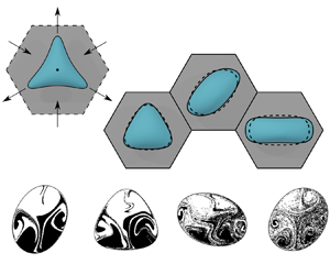
To model the branch intersection, we consider a hexagonal prism as our computational domain. The problem geometry, as well as a sample simulation of a deformable droplet in such geometry, can be seen in figure 1. In this geometry, the parallel top and bottom hexagonal panels correspond to the rigid, impenetrable walls of the microfluidic channel, whereas the six rectangular side panels correspond to the connections of the inlet/outlet branches with the intersection region. The flow rates at each branch, labelled  $Q_i$, can be changed with time almost independently, with the only constraint being mass conservation. We place the origin of the coordinate system at the geometric centre of the intersection, as indicated in figure 1(b).
Geometry used for the numerical simulations of a droplet in a Stokes trap. The simplified computational domain shown in (b) is a hexagonal prism corresponding to the intersecting region (B) of the multiple rectangular channel branches (A) in a microfluidic chip (C), illustrated in (a). The origin of the coordinate system, denoted as  $O$ in (b), is placed at the geometric centre of the hexagonal prism. (c) A more realistic computational domain, considering the channel branches combined with a moving frame $S_{\infty }^{{MF}}$ (as shown in Roure, Zinchenko & Davis Reference Roure, Zinchenko and Davis2023) to reduce computational times. The flow velocity at the entrance of each rectangular panel is given by a Boussinesq velocity profile with prescribed fluxes $Q_i$, which can be changed dynamically.

As simplified boundary conditions, we assume that the flow velocity profiles at the inlets/outlets of the hexagonal intersection region given by the Boussinesq solution for a rectangular channel and that there is no slip at the channel's top and bottom panels. We note that this formulation is different from the one in our previous work (Roure et al. Reference Roure, Zinchenko and Davis2023), where a moving frame (i.e. a small computational domain that follows the droplet throughout its motion) is used to reduce computational times for simulations of droplets in microfluidic channels. Further considerations regarding this simplified computational domain and comparison with extended computational geometries that include the rectangular branches (see figure 1c) using the algorithm from Roure et al. (Reference Roure, Zinchenko and Davis2023) are provided in § 2.1. The volumetric flow rate through each branch is prescribed and can be changed dynamically. The non-dimensionalization of the problem is made by using the inlet width  $W$ as the length scale, and a characteristic average velocity $U_{{av}}^B \equiv |Q|/(HW)$ to scale the velocity and potential densities, where $Q$ is a characteristic volumetric flow rate, and $H$ is the depth of the microfluidic channel. The choice of the flow rate $Q$ is made in a way such that, for a given characteristic flow mode, the average velocity of one of the branches is equal to unity.
As we consider the creeping-flow regime, the velocity on the drop interface is given by the solution of the following set of non-dimensional boundary-integral equations (Roure et al. Reference Roure, Zinchenko and Davis2023):
 \begin{align} \boldsymbol{u}(\kern0.7pt\boldsymbol{y}) &= \dfrac{2}{\lambda + 1} \left[ 2\int_{S_{\infty}} \boldsymbol{n}(\boldsymbol{x}) \boldsymbol{\cdot} \boldsymbol{\tau}(\boldsymbol{x} - \boldsymbol{y}) \boldsymbol{\cdot} \boldsymbol{q}(\boldsymbol{x}) \,{\rm d}S_{\boldsymbol{x}} + \boldsymbol{F}(\kern0.7pt\boldsymbol{y}) \right]\nonumber\\ &\quad+ 2\,\dfrac{\lambda - 1}{1 + \lambda} \int_{S_{d}} \boldsymbol{n}(\boldsymbol{x}) \boldsymbol{\cdot} \boldsymbol{\tau}(\boldsymbol{x} - \boldsymbol{y}) \boldsymbol{\cdot} \boldsymbol{u}(\boldsymbol{x}) \,{\rm d}S_{\boldsymbol{x}}, \end{align}
for  $\boldsymbol {y}$ on the drop surface $S_d$, and
 \begin{align} \boldsymbol{q}(\kern0.7pt\boldsymbol{y}) &= \boldsymbol{u}^{\infty}(\kern0.7pt\boldsymbol{y}) - 2 \int_{S_{\infty}} \boldsymbol{n}(\boldsymbol{x}) \boldsymbol{\cdot} \boldsymbol{\tau}(\boldsymbol{x} - \boldsymbol{y}) \boldsymbol{\cdot} \boldsymbol{q}(\boldsymbol{x}) \,{\rm d}S_{\boldsymbol{x}} - \boldsymbol{F}(\kern0.7pt\boldsymbol{y})\nonumber\\ &\quad- (\lambda - 1) \int_{S_{d}} \boldsymbol{n}(\boldsymbol{x}) \boldsymbol{\cdot} \boldsymbol{\tau}(\boldsymbol{x} - \boldsymbol{y}) \boldsymbol{\cdot} \boldsymbol{u}(\boldsymbol{x})\,{\rm d}S_{\boldsymbol{x}} - \dfrac{\boldsymbol{n}(\kern0.7pt\boldsymbol{y}) }{|S_{\infty}|} \int_{S_{\infty}} \boldsymbol{n}(\boldsymbol{x}) \boldsymbol{\cdot} \boldsymbol{q}(\boldsymbol{x})\,{\rm d}S_{\boldsymbol{x}}, \end{align}
for  $\boldsymbol {y}$ on the channel surface $S_{\infty }$. Here, $\lambda = \mu _d/\mu$ is the ratio between the drop viscosity and the viscosity of the surrounding fluid, $\boldsymbol {n}$ is the outward unit normal vector, $\boldsymbol {\tau }(\boldsymbol {r}) = 3 \boldsymbol {rrr}/(4 {\rm \pi}r^5)$ is the fundamental stresslet, $\boldsymbol {q}$ is a potential density (to be found) on the surfaces of the channel, and
 \begin{equation} \boldsymbol{F}(\kern0.7pt\boldsymbol{y}) = \frac{2}{Ca}\int_{S_{d}} \kappa(\boldsymbol{x})\, \boldsymbol{G}(\boldsymbol{x}-\boldsymbol{y}) \boldsymbol{\cdot} \boldsymbol{n}(\boldsymbol{x}) \, {\rm d}S_{\boldsymbol{x}} \end{equation}
for a neutrally buoyant droplet, where  $Ca = \mu U^B_{{av}}/\sigma$ is the capillary number, which measures the ratio between flow and interfacial-tension effects, $\kappa$ is the local mean curvature, $\sigma$ is the interfacial tension (assumed constant), and $\boldsymbol {G}(\boldsymbol {r}) = -(\boldsymbol {I}/r + \boldsymbol {rr}/r^3)/(8 {\rm \pi})$ is the Green's function for Stokes flow. Also note that, in contrast to our prior work (Roure et al. Reference Roure, Zinchenko and Davis2023), the potential density $\boldsymbol {q}$ also includes the undisturbed flow representation, in a way such that the undisturbed velocity $\boldsymbol {u}^{\infty }$ appears in the boundary-integral equation on the channel boundary, where the velocity is known from the boundary conditions. More explicitly, the equivalence between the two formulations can be obtained by making the transformation $\boldsymbol {q} \to \boldsymbol {q}+\boldsymbol {q}_{\infty }$, where $\boldsymbol {q}_{\infty }$ is the potential density associated with the double-layer representation of the undisturbed flow.
The two boundary-integral equations (2.1) and (2.2) are solved simultaneously by discretizing both the drop interface and channel boundaries, and solving the resulting finite system of linear equations using biconjugate-gradient iterations (see Roure et al. (Reference Roure, Zinchenko and Davis2023) for more details about the numerical method). The discretization of the drop interface, which we consider to always start from a spherical shape with radius  $a$, follows the icosahedron/dodecahedron-based approach from Zinchenko, Rother & Davis (Reference Zinchenko, Rother and Davis1997). The triangulation of the channel top and bottom panels uses a combination of Monte Carlo methods for disk packing and Delaunay triangulation described in Roure et al. (Reference Roure, Zinchenko and Davis2023). The calculation of the mean curvature and the outward normal vector $\boldsymbol {n}$ is done by using the best-paraboloid-spline method of Zinchenko & Davis (Reference Zinchenko and Davis2000). Further details about the boundary-integral formulation and the numerical methods can be found in our previous work (Roure et al. Reference Roure, Zinchenko and Davis2023).
For the mixing studies presented in § 4, we also need to calculate the velocity inside the droplets. To this end, a generalized double-layer representation for the internal flow (Pozrikidis Reference Pozrikidis1992; Kim & Karrila Reference Kim and Karrila2013) is used:
 \begin{equation} \boldsymbol{u}^{(i)}(\kern0.7pt\boldsymbol{y}) = 2 \int_{S_d} \boldsymbol{n}(\boldsymbol{x}) \boldsymbol{\cdot} \boldsymbol{\tau} (\boldsymbol{x} - \boldsymbol{y}) \boldsymbol{\cdot} \boldsymbol{\mathcal{Q}}(\boldsymbol{x}) \,{\rm d}S_{\boldsymbol{x}}, \end{equation}
where a potential density  $\boldsymbol {\mathcal {Q}}$ can be calculated by solving the partially deflated boundary-integral equation
 \begin{align} \boldsymbol{u}(\kern0.7pt\boldsymbol{y}) = 2 \int_{S_d} \boldsymbol{n}(\boldsymbol{x}) \boldsymbol{\cdot} \boldsymbol{\tau} (\boldsymbol{x} - \boldsymbol{y}) \boldsymbol{\cdot} \boldsymbol{\mathcal{Q}}(\boldsymbol{x}) \,{\rm d}S_{\boldsymbol{x} } + \boldsymbol{\mathcal{Q}}(\kern0.7pt\boldsymbol{y}) + \frac{\boldsymbol{n}(\kern0.7pt\boldsymbol{y})}{S_d} \int_{S_d} \boldsymbol{\mathcal{Q}}(\boldsymbol{x}) \boldsymbol{\cdot} \boldsymbol{n}(\boldsymbol{x}) \,{\rm d}S_{\boldsymbol{x}}, \quad \boldsymbol{y} \in S_d, \end{align}
on the drop surface. Note that (2.5) has the same form as the boundary-integral equation for the undisturbed channel flow in Roure et al. (Reference Roure, Zinchenko and Davis2023). Here, the surface velocity is given by the solution of the first boundary-integral problem (i.e. (2.1) and (2.2)). Equation (2.5) is discretized using a linear quadrature (Zinchenko et al. Reference Zinchenko, Rother and Davis1997) and solved numerically using the method of generalized minimal residuals. For the evaluation of the double-layer integrals in (2.4) and (2.5), we use the standard singularity/near-singularity subtraction from Loewenberg & Hinch (Reference Loewenberg and Hinch1996).
2.1. Effects of boundary condition simplification
As mentioned in the previous section, most of the simulations in this paper consider the channel intersection as the computational geometry with Dirichlet boundary conditions at its inlets and outlets given by the Boussinesq flow in a straight, rectangular channel. Although this configuration is more physically accurate than the external flow used in previous theoretical works for the Stokes trap (e.g. Lin et al. Reference Lin, Kumar, Richter, Wang, Schroeder and Narsimhan2021), these boundary conditions should be imposed on a section of a channel branch away from the intersection to more accurately model typical experimental set-ups, either by simulating the droplet in the full microfluidic domain or by using a moving-frame construction like the one described in Roure et al. (Reference Roure, Zinchenko and Davis2023) (see figure 1c), in which the frame changes with time as the drop moves and/or deforms. When doing the latter, it is still possible to implement the methods proposed in the present paper, including the control algorithm, by using a transient mode superposition of pre-calculated potential densities. Here, we briefly assess the main quantitative differences that may appear when considering the alternative inlet/outlet boundary conditions on sections of the branches away from the intersection.
We start by looking at the effect of branch length (i.e. the distance from the intersection to where we apply the boundary conditions within the rectangular inlet/outlet branches) on the undisturbed flow (i.e. without the droplet). Figure 2(a) shows a comparison between the undisturbed flow field for the hexagonal prism domain shown in figure 1(b) (in black) and the flow field of the full geometry shown in figure 1(a) (in blue), for a channel with dimensionless branch lengths  $L = 2.0$. As seen by the results in figure 2, although the flow fields are qualitatively similar, they present notable quantitative differences that arise between the direct application of the Boussinesq boundary conditions at the hexagonal computational cell versus at a dimensionless distance $L = 2.0$ from the hexagonal intersection. As expected, and seen in figure 2(b), increasing the length of the channel branches results in much smaller discrepancies between the velocity fields. For $L = 1.5$, these differences become very small, with discrepancies of less than $0.5\,\%$ for the bulk of the channel (except for the origin, where the velocity is zero), indicating that the limit of very long inlet/outlet channels is well reached for $L = 2.0$. As the results in this paper are more focused on the effects of flow-mode superposition on the drop deformation and mixing dynamics than the modelling of a more physically accurate channel flow, we use primarily the simplified hexagonal construction shown in figure 1(b). However, as quantitative differences in drop shape may arise from considering the full channel geometry, in § 3 we address some of these differences between the simplified external flow field and simulations of a droplet inside a full-channel representation of a Stokes trap with branch size $L = 2.0$ performed using the moving-frame approach from Roure et al. (Reference Roure, Zinchenko and Davis2023). As in our previous work, the computational frame expands as the drop stretches, and it moves if conditions are such that the drop drifts from its initial location. Overall, the results for the full-channel simulations are qualitatively similar to those for the simplified geometry, but with less-deformable droplets. As we show in the next section, this discrepancy is characterized by a quantitative difference in the components of the spherical-harmonic decomposition of the drop shape. These discrepancies are usually small for smaller droplets, but can become up to ${\sim }40\,\%$ in some extreme cases for larger, more-deformable droplets.
Effect of channel branch length on background flow in a Stokes trap. (a) Qualitative comparison between the vector fields for  $L = 0$ (black) and $L = 2.0$ (blue) at the same points. (b) Colour maps show the scalar discrepancy between the vector fields for different channel branch lengths.

3. Flow modes and drop deformation
Many works in the literature analyse drop and vesicle behaviour under simple-shear and extensional flows (e.g. Loewenberg & Hinch Reference Loewenberg and Hinch1996, Reference Loewenberg and Hinch1997; Zinchenko et al. Reference Zinchenko, Rother and Davis1997; Oliveira & Cunha Reference Oliveira and Cunha2015). More recently, the four-branch Stokes trap has been used to perform extensional-flow experiments with vesicles Kumar et al. (Reference Kumar, Richter and Schroeder2020a). In the six-branch Stokes trap, the higher number of degrees of freedom allows us to locally reproduce not only a pure-extensional flow but also other ‘classical’ flow modes such as extensional and quadratic flows, by manipulating the flow rates  $Q_i$ in the branches. As an example, figure 3 shows some of these different flow modes and the deformation response of a droplet to each one. The three flow modes represented by figures 3(a,b,c) are given, respectively, by
 $$\begin{gather} \boldsymbol{Q}_{{tri}} = (1,-1,1,-1,1,-1), \end{gather}$$
 $$\begin{gather}\boldsymbol{Q}_{{sh}} = (0,1,-1,0,1,-1) \end{gather}$$
and
 \begin{equation} \boldsymbol{Q}_{{ext}} = (2,-1,-1,2,-1,-1). \end{equation}
We call these modes (a) tri-axial extension, (b) shear, and (c) extension, respectively. Note that the extensional mode can be obtained by a ‘symmetrization’ of the shear mode, namely,  $\boldsymbol {Q}_{{ext}} = \mathcal {S}\boldsymbol {Q}_{{sh}} - \mathcal {S}^2\boldsymbol {Q}_{{sh}}$, where $\mathcal {S}$ is the shift operator defined by
 \begin{equation}
\mathcal{S}(\boldsymbol{Q})_i = \left\{\begin{array}{@{}ll@{}} Q_{i+1}, &
\text{for }i < 6, \\
Q_{1}, & \text{for }i = 6.
\end{array}\right.
\end{equation}
\begin{equation}
\mathcal{S}(\boldsymbol{Q})_i = \left\{\begin{array}{@{}ll@{}} Q_{i+1}, &
\text{for }i < 6, \\
Q_{1}, & \text{for }i = 6.
\end{array}\right.
\end{equation}
The shift operator corresponds to a  $60^{\circ }$ rotation of a given flow configuration. By symmetry, we have $\mathcal {S}^2\boldsymbol {Q}_{{tri}} = \boldsymbol {Q}_{{tri}}$ and $\mathcal {S}^3\boldsymbol {Q}_{{sh}} = \boldsymbol {Q}_{{sh}}$. Animated versions of these drop deformation modes can be found in the supplementary material available at https://doi.org/10.1017/jfm.2024.289.
Different drop deformation modes produced by the Stokes trap. The undisturbed flow for each mode is shown in (a ii–c ii), whereas the shape responses are shown in (a i–c i). For the simulations, we consider  $H = 1$, $a = 0.5$, $Ca = 0.1$, $\lambda = 1$, and (a) $\boldsymbol {Q} = \boldsymbol {Q}_{{tri}}$, (b) $\boldsymbol {Q} = \boldsymbol {Q}_{{sh}}$, and (c) $\boldsymbol {Q} = \boldsymbol {Q}_{{ext}}$. The solid shapes are for simulations of droplets in the simplified hexagonal geometry, whereas the dashed shapes are for simulations considering a full channel geometry with $L = 2$. All the shapes are given at the same time $t = 0.2$. The numbers in (a ii–c ii) correspond to the values of the flux $Q_i$ at each face for each mode.

The simulations in figure 3 were performed by considering an initially spherical droplet of dimensionless radius  $a = 0.5$ starting at the centre of the channel. The results considering a full-channel geometry (cf. § 2.1), represented by the dash contours, show qualitatively similar results, but with slightly smaller deformation. (These discrepancies in drop deformation are characterized quantitatively in § 3.1.) For less-deformable droplets (e.g. small $Ca$ and $\lambda$), the drop will eventually reach an equilibrium shape. However, in both experiments and numerical simulations, this equilibrium point might be unstable, meaning that small changes in the drop initial position may lead to the drop escaping the Stokes trap; this situation is shown in figure 4(b). To overcome this issue, we introduce a simple linear feedback controller to keep the droplet at the centre of the channel. To control drop translation, it is useful to know how to induce drop translation in the $x$ and $y$ axes individually, as these translation modes can combine linearly for Stokes flow to induce translation in any arbitrary direction in the $xy$ plane. One way that these modes can be achieved is shown in figure 4(a). Considering the translation flow modes
 \begin{equation} \boldsymbol{Q}_h = (0,-1,-1,0,1,1) \end{equation}
and
 \begin{equation} \boldsymbol{Q}_v= (1,0,0,-1,0,0), \end{equation}
the controlled flow rates are given by
 \begin{equation} \boldsymbol{Q} = \boldsymbol{Q}_0 - \left[ \alpha \boldsymbol{Q}_h \beta \boldsymbol{Q}_v \right] \begin{bmatrix} x_c \\ y_c \end{bmatrix}, \end{equation}
where  $\boldsymbol {Q}_0$ is the applied flux configuration in the absence of control, $[ \alpha \boldsymbol {Q}_h \beta \boldsymbol {Q}_v ]$ is a block matrix whose columns are given by $\alpha \boldsymbol {Q}_h$ and $\beta \boldsymbol {Q}_v$, and $\boldsymbol {x}_c = (x_c,y_c,z_c)$ is the surface centroid, given by
 \begin{equation} \boldsymbol{x}_c = \frac{1}{S_d} \int_{S_d} \boldsymbol{x} \,{\rm d}S, \end{equation}
with  $\alpha$ and $\beta$ being constants related to the strength of the control. When the droplet is not centred in the Stokes trap, the flux correction in (3.7) adds a counter-flux contribution, proportional to the droplet displacement from the centre of the channel, which moves the droplet towards the intersection centre by combining the translation modes (see figure 4).
Application of the linear feedback control. (a) Horizontal and vertical flow modes used for the control implementation. (b) Drop behaviour in the (ii,iii) presence and (iv,v) absence of control in numerical simulations for  $a = 0.4$, $Ca = 0.1$, $\lambda = 1$, and starting centre position $\boldsymbol {x}_c = (0.1 \cos (0.5),0.1 \sin (0.5),0)$, for (i) $t = 0$, (ii,iv) $0.25$, (v) $1.5$, and (iii) steady state.

For general applications, one has to be careful in choosing the constants  $\alpha$ and $\beta$, as strong additional fluxes may lead to drop breakup, and weak additional fluxes might not be strong enough to counteract the flux $\boldsymbol {Q}_0$, leading to a small region of effectiveness of the control algorithm near the centre of the intersection region. For the purpose of the simulations in this paper, the values $\alpha = \beta = 1$ have been found to perform well. It is also noted that if the origin is not an equilibrium point for the flux configuration $\boldsymbol {Q}_0$, or if one wants the drop centre to be positioned at a different target position, then an integral component should be added to (3.7). To illustrate the effectiveness of the simple proportional control algorithm, figure 4(b) shows the effect of the controller on the motion of a droplet starting off-centre. In the absence of a controller, the droplet tends to escape the channel, as shown in figures 4(b iv–v). The extension in this regime can also lead to drop breakup. In contrast, when the controller is turned on (figures 4b i–ii), the additional fluxes move the drop to the centre of the channel, keeping its position and shape stable.
3.1. Characterizing drop deformation via spherical harmonics
Often in the literature, drop deformation is characterized by parameters such as the Taylor deformation, which measures the deviation of a drop from its spherical equilibrium shape. From figure 3, it is clear that the different drop shapes induced by the distinct flow modes show substantial variation. Hence to properly describe drop deformation, we need a more precise way to characterize the deformed drop shape. One way to do this, valid for star-shaped drop geometries, is to decompose the shape of the droplet in spherical harmonics. Namely, the shape of the droplet is described by the function  $r(\theta,\varphi )$, where $r$ is the spherical radial coordinate from the drop centre, and $\varphi$ and $\theta$ are the azimuthal and polar angles, respectively. This function can be decomposed as
 \begin{equation} r(\theta,\varphi) = \sum_{\ell,m} c_{\ell m}\,Y_{\ell}^{m}(\theta,\varphi), \end{equation}
where  $Y_{\ell }^m(\theta,\varphi )$ are the normalized spherical harmonics, and the coefficients $c_{\ell m}$ are
 \begin{equation} c_{\ell m} = \int_{S^2} r(\theta,\varphi)\,\bar{Y}_{\ell}^{m}(\theta,\varphi) \,{\rm d}\varOmega, \end{equation}
with  $S^2$ the unit sphere, and overbar denoting complex conjugation. Numerical implementation of (3.10) consists of first projecting the unstructured drop mesh on the unit sphere and using a linear quadrature (e.g. Zinchenko et al. Reference Zinchenko, Rother and Davis1997).
As an example of harmonic decomposition, we examine the case of a droplet undergoing a tri-axial extensional flow shown previously in figure 3. Figure 5 shows numerical results for (a) the harmonic decomposition of drop shape in a tri-axial extensional flow mode, and (b) reconstruction of drop shape by using the first few harmonics. As the tri-extensional flow is locally quadratic, we expect the main excited harmonic to be  $Y_{33}$, as in the regime of small deformations. Indeed, as shown in figure 5(a), besides $Y_{00}$, the largest harmonic in the spectrum is $Y_{33}$, followed by $Y_{66}$. All other harmonics are substantially smaller, which is supported by the fact that we can reconstruct the drop shape with good accuracy by using only three harmonics, as shown in figure 5(b).
Harmonic decomposition of the shape of a droplet in a Stokes trap undergoing a tri-axial extensional flow for  $Ca = 0.1$, $\lambda = 1$, $H = 1$ and $a = 0.5$. The results show (a) the evolution of the $Y_{33}$ and $Y_{66}$ harmonics with time as the drop extends, and (b) the reconstruction of drop shape from the three main harmonics for $t = 0.25$. The dashed curves in (a) are the same harmonics for a full-channel simulation with branch length $L = 2.0$, whereas the solid curves are for the simplified hexagonal geometry. The dashed shapes in (b) are the numerical drop shape, whereas the solid lines are the harmonic approximations. The meshed geometry in (b) is a three-dimensional visualization of the harmonic reconstruction using the main three modes. (c) A comparison between the simulations in the simplified hexagonal channel (solid contours) and full channel (dashed contours) from (a).

The results shown in figure 5 indicate that a good parameter to measure drop deformation in a tri-axial extensional flow is the imaginary part of  $c_{33}$. The results for the full-channel simulations display a similar increasing behaviour, although with smaller drop deformation, which is characterized by lower absolute values of the harmonic coefficients $c_{33}$ and $c_{66}$. This discrepancy in deformation also leads to a difference in long-time behaviour, as the droplet in the full-channel simulation will eventually reach a stationary state, whereas the droplet in the simplified geometry escapes the hexagonal region in three different directions, suggesting that it will eventually break up. Hence we can perform numerical experiments with our trapped droplet. One possible example of such a numerical experiment is an oscillatory flow of the form
 \begin{equation} \boldsymbol{Q}_0(t) = \boldsymbol{Q}_{{tri}}\cos(\omega t), \end{equation}
where  $\omega$ is the inlet frequency. Figure 6(a,b) show the response of $c_{33}$, normalized by the drop radius $a$, to the oscillatory tri-extensional flow for $Ca = 0.1$, $\lambda = 1$, $H = 1$ and $\omega = 3$ for different values of drop radius $a$. The vertical dashed lines in figure 6 indicate the points in time where $\boldsymbol {Q} = \boldsymbol {0}$. As expected, larger droplets are more deformable, which results in a larger values of $\text {Im}(c_{33})/a$. Moreover, for droplets with radii $a=0.4$ or less (figure 6a), besides an initial transient regime, the harmonic response displays a sinusoidal behaviour slightly out of phase with the flux, indicating a small lag in the drop response, which is expected given the elastic character of the interfacial tension. We also note that drop size slightly affects the phase of drop oscillation. For the full channel simulations, shown as the dashed curves, we again observe a smaller deformation, but with the same qualitative trends. For $a = 0.5$, for the full-channel simulations (dashed curves), we observe a similar trend, with a harmonic deformation. However, for the hexagonal channel simulation, where deformations are larger, we observe non-sinusoidal oscillations, as shown in figure 6(b), indicating a ‘nonlinear’ response. Note that the oscillations in figure 6(b), besides displaying non-harmonic behaviour, also have slightly increasing peaks, indicating that either a larger time is required for the droplet oscillation to reach periodic behaviour or these oscillations are unstable (in the sense that they may potentially lead to drop breakup).
Numerical results for the imaginary part of the harmonic amplitude  $c_{33}$, normalized by the drop radius, versus time for a droplet undergoing an oscillatory tri-axial extensional flow $\boldsymbol {Q}_0 = \boldsymbol {Q}_{{tri}} \cos (\omega t)$. The results consider $Ca = 0.1$, $\lambda = 1$, $H = 1$, $\omega = 3$, and (a) $a = 0.25, 0.3, 0.4$, and (b) $a = 0.5$. (c) The harmonic response for $a = 0.4$, and $\omega = 0.0, 0.5, 1.0, 1.5, 2.0, 2.5$. (d) The frequency response for the drop sizes in (a). The solid curves are the results for the simplified geometry, whereas the dashed curves in (a,b,d) were obtained by a full-channel simulation with branch length $L = 2.0$. The dotted curves in (a,b) indicate the amplitude of the flux $Q_1$, whereas the vertical lines indicate the times where $\boldsymbol {Q} = \boldsymbol {0}$.

Besides drop size and physical parameters such as  $Ca$ and $\lambda$, an important quantity in oscillatory flows that influences the extension of drop deformation is the oscillation frequency $\omega$. The results in figures 6(c) and 6(d) show, respectively, the influence of different frequencies on the harmonic $c_{33}$, and a frequency ramp for oscillation amplitudes for different drop sizes. As expected from classical results for droplets under simple oscillatory extensional flows, smaller oscillation frequencies result in larger drop deformations, which are characterized by larger values of $\text {Im}(c_{33})$.
We can also use our method to simulate the stretching and relaxation behaviour of a droplet under step-strain conditions, similar to the vesicle experiments performed in Kumar et al. (Reference Kumar, Richter and Schroeder2020b). Besides, the decomposition in spherical harmonics allows us to quantify drop deformation for both regular extensional ( $\boldsymbol {Q}_{{ext}}$) and tri-extensional ( $\boldsymbol {Q}_{{tri}}$) flow modes. To illustrate this type of numerical experiment, figure 7 shows numerical results for a droplet undergoing a step-strain, tri-axial extension for $Ca = 0.1$, $\lambda = 1$, $H = 1$ and $a = 0.5$. The flow configuration is given by $\boldsymbol {Q}_{{tri}}$ for $t \le 0.2$, and $\boldsymbol {0}$ for $t >0.2$. For $t \le 0.2$, the drop experiences a tri-axial extension that is characterized by an increase in the $Y_{33}$ harmonic, as shown in figure 5. As the external flow suddenly stops, the droplet shape relaxes towards its initial spherical configuration. The results for the full-channel simulation, represented by the dashed curve, display a similar qualitative behaviour, with amplitudes approximately 30 % lower.
Numerical results for the  $Y_{33}$ harmonic response of a droplet undergoing a step tri-axial strain with $Ca = 0.1$, $\lambda = 1$, $a = 0.5$, $H = 1$, and $\boldsymbol {Q}_0 = \boldsymbol {Q}_{{tri}}$ for $t \le 0.2$, and $\boldsymbol {Q} = \boldsymbol {0}$ for $t > 0.2$. The result represented by the solid curve is for the simplified hexagonal domain, whereas the dashed curve is the result for the full-channel geometry with branch length $L = 2.0$.

3.2. Mode combination and shape manipulation
As shown in the previous subsection, subjecting the droplet to different flow modes in the Stokes trap may excite specific harmonics on the drop interface – a feature that can be used for shape manipulation. These modes can also be combined together to produce more complex drop shapes. To illustrate this observation, figure 8 shows numerical simulations for droplets undergoing a combination of (a) shear + tri-axial extension and (b) extension + tri-axial extension for  $Ca = 0.05$, $\lambda = 1$ and different drop radii $a$.
$a$.
Numerical results for drop shapes resulting from combinations (a) tri-extensional + shear and (b) tri-extensional + extensional flow modes, for  $Ca = 0.05$, $\lambda = 1$, $H = 1$, and different drop radii. The solid contours represent steady shapes, whereas the long-dashed contours, corresponding to (a) $t = 0.925$ and (b) $t = 0.35$, represent larger drops that eventually escape the intersection, possibly leading to breakup. The short-dashed contours (overlapping the solid contours) were obtained by the harmonic superposition of the half modes from table 1, and essentially coincide with the full simulations.

The results shown in figure 8 show that the combination of different flow modes can result in asymmetric drop shapes such as the ones shown in figure 8(a), while the droplet is kept at the centre of the channel by the controller. This asymmetry is even more pronounced for larger droplets. However, above a certain radius threshold, the droplet becomes too elongated, escaping the intersection, possibly leading to breakup. For small radii  $a$, for which the droplet undergoes small deformations, we observe a linear deformation regime, where the harmonics superpose linearly. This linear superposition for small droplets is shown in table 1, which gives numerical results for the main spherical harmonics present in the steady shapes shown in figure 8, with additional results from numerical simulation using the isolated ‘half modes’ $\boldsymbol {Q}_{{tri}}/2$, $\boldsymbol {Q}_{{ext}}/2$ and $\boldsymbol {Q}_{{sh}}/2$. The numerical results show that for small droplets (e.g. $a = 0.3$), the harmonic spectrum of the final shape due to a combined mode seems to be given by a linear superposition of the isolated modes, as expected from the theory of small deformations (Leal Reference Leal2007). In contrast, as in the case for the oscillatory flow, we start to observe a nonlinear behaviour for large droplets, which is characterized by the lack of linear harmonic superposition and the presence of extra harmonics. As an example, we can start to see some small discrepancies for $a= 0.4$ between the final harmonics and the ones from the isolated modes. This linear superposition of harmonic modes for moderate deformations is further supported by the reconstruction of the final shape by a linear combination of the half modes, which is shown by the short-dashed contours in figure 8. For $a = 0.5$, as in the harmonic response to the oscillatory flow presented in § 3.1, linearity is no longer observed.
Numerical results for the steady-state harmonic decomposition of different simple and combined flow modes for  $Ca = 0.05$, $\lambda = 1$ and $H = 1$. The results are rounded to three decimal places.

3.3. A hydrodynamic ‘three-phase rotor’
Drop rotation often plays an important role in improving the chaotic mixing inside the droplets (Stone, Nadim & Strogatz Reference Stone, Nadim and Strogatz1991), which is crucial for applications in drop-based microreactors. It is known from the literature that droplets in a simple shear flow display a tumbling motion for high viscosity ratios (Bilby & Kolbuszewski Reference Bilby and Kolbuszewski1977; Wetzel & Tucker Reference Wetzel and Tucker2001; Oliveira & Cunha Reference Oliveira and Cunha2015). In contrast, droplets with low viscosity ratios reach a steady-state deformation, where they present a ‘tank-treading’ motion (Kennedy, Pozrikidis & Skalak Reference Kennedy, Pozrikidis and Skalak1994). Whereas a four-roll mill can produce rotational flow, it is difficult, and possibly not feasible, to produce a flow that is locally rotational at the centre of a Stokes trap. For example, the model used by Shenoy et al. (Reference Shenoy, Kumar, Hilgenfeldt and Schroeder2019) represents the external flow inside a Stokes trap as a superposition of potential sources, which is irrotational. In fact, the mode shown in figure 3(b), which we labelled as ‘shear’, is locally an extensional flow.
However, the six-branch Stokes trap allows us to generate a rotating extensional external flow by combining the three different possible modes for the ‘shear’ mode,  $\boldsymbol {Q}_{{sh}}$, $\mathcal {S}\boldsymbol {Q}_{{sh}}$ and $\mathcal {S}^2 \boldsymbol {Q}_{{sh}}$, off phase by $2 {\rm \pi}/3$, in the form
 \begin{equation} \boldsymbol{Q}_{{rotor}} = \tfrac{1}{3} \left[ \boldsymbol{Q}_{{sh}} \cos(\omega t) + \mathcal{S} \boldsymbol{Q}_{{sh}} \cos(\omega t + 2 {\rm \pi}/3) + \mathcal{S}^2 \boldsymbol{Q}_{{sh}} \cos(\omega t + 4 {\rm \pi}/3) \right]. \end{equation}
Note, for example, that for  $t = {\rm \pi}/2$, $\boldsymbol {Q}_{{rotor}} \propto \boldsymbol {Q}_{{ext}}$. Numerical results for a single droplet in a Stokes trap undergoing the external flow produced by the flux configuration described in (3.12) with $\omega = 3$ are shown in figure 9. The droplet starts with a spherical shape and undergoes a transient extension regime until it reaches a periodic regime, with frequency $\omega$, similar to the wobbling motion observed in high-viscosity-ratio droplets undergoing a simple shear flow. An animated version of the drop motion can be found in the supplementary material.
Numerical results for a droplet undergoing a three-phase extensional flow for  $Ca = 0.05$, $\lambda = 1$, $a = 0.4$, $H = 1$ and $\omega = 3$. The motion of the drop is comprised of a short transient regime, shown in (a), where the droplet transitions from a spherical to an ovoid shape, and a periodic wobbling regime, shown in (b). The timeline at the bottom displays the full motion of the droplet. The solid drop shape for each part represents the first drop configuration for that part (i.e. first and fourth panels), whereas the dashed shape corresponds to the last configuration displayed on the timeline for that part (i.e. third and seventh panels). (c) The effect of the frequency $\omega$ on the maximum amplitude of the $c_{22}$ harmonic.

From the frequency response curve shown in figure 9(c), we see that, as in the case of the oscillatory tri-axial flow in § 3.1, the increase in rotation frequency leads to a smaller drop deformation. One interesting feature of this type of flow is that at each time step, the external flow acts similarly to an extensional flow. As the internal flow inside a droplet undergoing an external extensional flow has four circulation regions, a continuously rotating extensional flow will continuously change these invariant mixing regions, making it possible to observe effective mixing inside the droplet. In the next section, we investigate how this rotating flow mode may be used to produce active mixing inside the droplet.
4. Chaotic mixing inside droplets
4.1. General remarks
Besides influencing drop shape and deformation, the different flow modes investigated in the prior portion of this paper also affect the internal circulation. In this section, we investigate how these induced internal flows influence mixing inside the droplets.
Due to the large number of microfluidic applications, chaotic mixing inside droplets has been investigated extensively in the literature, both theoretically and experimentally (Sarrazin et al. Reference Sarrazin, Loubiere, Prat, Gourdon, Bonometti and Magnaudet2006; Blanchette Reference Blanchette2010; Zhao et al. Reference Zhao, Riaud, Luo, Jin and Cheng2015; Chen et al. Reference Chen, Zhao, Wang, Zhu, Tian, Xu, Wang and Huang2018). For example, chaotic mixing inside isolated spherical droplets induced by linear external flows was investigated by Stone et al. (Reference Stone, Nadim and Strogatz1991), inducing chaos by applying external, non-aligned extensional and rotation flows. For quadratic flows, even earlier results by Bajer & Moffatt (Reference Bajer and Moffatt1990) show a stretch-twist-fold chaotic dynamics. Later, Stone & Stone (Reference Stone and Stone2005) investigated a transient combination of shear and uniform flows to emulate the conditions in a typical microfluidic serpentine mixer. This work was also extended to direct numerical simulations of deformable two-dimensional droplets in a serpentine channel (Muradoglu & Stone Reference Muradoglu and Stone2005) using a finite-volume/front-tracking scheme. The characterization of mixing inside droplets in different microfluidic channels is still being explored (Fu et al. Reference Fu, Wang, Zhang, Bai, Jin and Cheng2019; Belousov et al. Reference Belousov, Filatov, Kukhtevich, Kantsler, Evstrapov and Bukatin2021; Cao et al. Reference Cao, Zhou, Yu and Liu2021). Recently, Gissinger, Zinchenko & Davis (Reference Gissinger, Zinchenko and Davis2021) used boundary-integral simulations to investigate mixing inside a droplet trapped in constrictions formed by rigid particles and fibres. Beyond the context of microchannels, the work by Watanabe, Hasegawa & Abe (Reference Watanabe, Hasegawa and Abe2018) also explored active mixing inside droplets in an acoustic trap.
Here, similarly to the previous work by Gissinger et al. (Reference Gissinger, Zinchenko and Davis2021), we use boundary-integral simulations to study the mixing dynamics inside the droplet in a Stokes trap. One of the advantages of boundary-integral methods for mixing simulations is that the velocity of the fluid at any point inside the droplet can be determined by the numerical evaluation of (2.4), without requiring interpolation. In contrast to the problem considered in Gissinger et al. (Reference Gissinger, Zinchenko and Davis2021), our droplet undergoes continuous deformation, not being confined to a steady state. To illustrate the velocity calculation inside the droplets for deformable droplets, figure 10(a) shows the short-time evolution of streamlines inside an initially spherical droplet. It reveals the formation of six circulation regions at the midplane  $z = 0$ inside a droplet undergoing a tri-axial extensional flow. At $t = 0$, the flow inside the droplet resembles the undisturbed external flow shown in figure 3(a). As the droplet deforms, we start to see six saddle-like fixed points moving from the drop centre towards its boundary, giving rise to the six circulation regions. For droplets with small deformations (e.g. $Ca \to 0$), this formation happens almost instantly. These circulation regions are very similar to those observed inside a spherical droplet subjected to an external quadratic flow.
Flow inside an initially spherical droplet subject to an external tri-axial extensional flow with  ${Ca = 0.1}$, $\lambda = 1$, $a = 0.4$ and $H = 1$. (a) The transient formation of six circulation regions inside the droplet. (b) The details of the mixing simulations, including the regions $V_{{dye}}$ (in black) and $V_{{clear}}$ (in white) used in the calculation of the mixing number. The final configuration is calculated by backtracing the centres of cells in a Cartesian grid to their initial positions.

Although there are multiple ways to characterize mixing in fluids, one that is particularly interesting in our case is the mixing number, introduced by Stone & Stone (Reference Stone and Stone2005). This particular choice comes from the visual intuitiveness of such a parameter, and its connection to the convective transport of a fluid region. This parameter was also shown to be correlated (or inversely correlated) to other quantities such as entropy, intensity of segregation, and other mixing quantifiers (Muradoglu & Stone Reference Muradoglu and Stone2005; Hoeijmakers et al. Reference Hoeijmakers, Araujo, van Heijst, Nijmeijer and Trieling2010; Gissinger et al. Reference Gissinger, Zinchenko and Davis2021; Roshchin & Patlazhan Reference Roshchin and Patlazhan2023). To illustrate the definition of this metric, we focus on the classical example of an initially spherical droplet with passive dye completely filling one of its hemispheres. This problem is illustrated in figure 10(b). As time passes, the dye is advected with the same velocity as the flow inside the droplet. As the dye is assumed to be non-diffusing, the sets  $V_{{dye}}$, consisting of the dyed points, and $V_{{clear}}$, consisting of the clear points, are disjoint. The mixing number is a measure of closeness between the two disjoint sets. In our specific case, we define it in the following grid-independent form:
 \begin{equation} m(t) = \frac{1}{a^2 V_d} \left[\int_{V_{{dye}}} d^2(\boldsymbol{x},V_{{clear}}) \,{\rm d} V + \int_{V_{{clear}}} d^2(\boldsymbol{x},V_{{dye}}) \,{\rm d} V \right], \end{equation}
where  $d^2(\boldsymbol {x},A) = \inf _{\boldsymbol {y}\in A} d^2(\boldsymbol {x},\boldsymbol {y})$ is the square of the distance between the point $\boldsymbol {x}$ and the set $A$. The normalization factor $a^2$ is used to make the mixing number non-dimensional and to avoid an extra drop-size dependency in $m(t)$. If the system is well mixed, then the two sets become strongly intertwined and the mixing number approaches zero, hence providing an inverse measure of mixing between the two sets.
In practical applications, as the nonlinear dynamics of the system must be solved numerically, the implementation of (4.1) is performed in a coarser domain given by a Cartesian grid formed by cubic cells of the same volume. Under these circumstances, the mixing number is given by
 \begin{equation} m(t) \approx \frac{1}{a^2 N_{g}} \sum_{k=1}^{N_{g}} d^2(\boldsymbol{x}_k,\text{Opp}(\boldsymbol{x}_k)), \end{equation}
which is the same expression as in Stone & Stone (Reference Stone and Stone2005). Here, the summation is over the grid cells,  $N_g$ is the total number of cells, $\boldsymbol {x}_k$ is the midpoint of a cell $k$, and
 \begin{equation}
\text{Opp}(\boldsymbol{x}) = \left\{\begin{array}{@{}ll@{}} V_{{dye}}, & \text{if} \ \boldsymbol{x} \in V_{{clear}},\\
V_{{clear}}, & \text{if} \ \boldsymbol{x} \in V_{{dye}},
\end{array}\right.
\end{equation}
\begin{equation}
\text{Opp}(\boldsymbol{x}) = \left\{\begin{array}{@{}ll@{}} V_{{dye}}, & \text{if} \ \boldsymbol{x} \in V_{{clear}},\\
V_{{clear}}, & \text{if} \ \boldsymbol{x} \in V_{{dye}},
\end{array}\right.
\end{equation}
where  $V_{{dye}}$ and $V_{{clear}}$ are the coarse-grained versions of their continuous counterparts. For a two-dimensional system, the definition of the mixing number (4.1) would be similar but with areas instead of volumes. Its numerical counterpart (4.2), however, would remain unaltered, with the exception that the Cartesian grid would now be two-dimensional.
The regions  $V_{{dye}}$ and $V_{{clear}}$ are determined by tracing the centre point of each cell to its starting position and using the initial condition for dye concentration (see figure 10b). This method is referred to as the backward Poincaré cell method (Wang et al. Reference Wang, Fan and Chen2001) and has been used in previous works to obtain graphical representations for the chaotic mixing inside droplets. For incompressible flows, such a method yields more accurate results for the mixing number when compared to forward propagation, as it consists in a direct discretization of the final concentration profile obtained by the method of characteristics for the advective transport equation (Roure & Davis Reference Roure and Davis2021). Namely, if the dye concentration $c(\boldsymbol {x},t)$ undergoes a purely advective transport, with $\partial c/\partial t + \boldsymbol {u} \boldsymbol {\cdot } \boldsymbol {\nabla } c = 0$ and initial condition $c_0(\boldsymbol {x})$, then the concentration at a time $t$ is given by $c_0(\varPsi _t^{-1} (\boldsymbol {x}))$, where $\varPsi _t$ is the time evolution of the dynamical system from a starting position at $t = 0$. Note that forward propagation is still necessary to calculate quantities such as the mixing entropy (Muradoglu & Stone Reference Muradoglu and Stone2005), which we do not explore in this work.
For calculation of both regular and backward trajectories, we use a second-order Runge–Kutta scheme. The fluid velocity field inside the droplet at each time step is calculated by the numerical evaluation of (2.4). To this end, the drop shapes and potential densities for the relevant time steps are pre-calculated and stored by solving the boundary-integral problem. To keep track of the points inside the droplet, we use an indicator function
 \begin{equation} I(\kern0.7pt\boldsymbol{y}) = \frac{1}{4 {\rm \pi}} \int_{S_d} \frac{\boldsymbol{n}(\boldsymbol{x})\boldsymbol{\cdot}(\boldsymbol{x} - \boldsymbol{y})}{\| \boldsymbol{x} - \boldsymbol{y} \|^3} \,{\rm d}S_{\boldsymbol{x}}, \end{equation}
which is 1 for  $\boldsymbol {y}\in V_d$, and 0 for $\boldsymbol {y} \notin V_d$. For drop-surface discretization into flat mesh triangles $\triangle$, each triangle contribution to (4.4) is simply the signed area of the spherical triangle obtained by projecting $\triangle$ onto the unit sphere centred at $\boldsymbol {y}$, and this area is found analytically from spherical trigonometry (as in Zinchenko & Davis Reference Zinchenko and Davis2013).
4.2. Mixing in deformable droplets
We now analyse how different flow modes may influence the mixing inside deformable droplets. As we are considering the droplet to be neutrally buoyant and centred at  $z = 0$, the plane $z = 0$ is a two-dimensional invariant manifold for all the flow modes considered in this paper. As the mixing in this two-dimensional submanifold often correlates with overall three-dimensional mixing inside the droplet (Stone & Stone Reference Stone and Stone2005), we focus our mixing analysis on the cross-section $z = 0$.
One of the main consequences of drop deformation is the breaking of the kinematic reversibility usually present in Stokes flows, which may improve the mixing inside the droplet for specific cases. To illustrate the effects of irreversibility, we return to the oscillatory flow problem discussed in § 3.1. For a perfectly spherical droplet (e.g.  $Ca = 0$), the linearity of Stokes equations implies that an oscillatory flow mode would not produce any type of effective mixing inside the droplet. Instead, all points would return to their initial position after one period. In contrast, for a deformable droplet, this kinematic symmetry is broken by the drop deformation, meaning that a given material point inside the droplet will display non-periodic dynamics, as illustrated in figure 11(a). This symmetry breaking is similar to that observed in the relative trajectories of particles leading to hydrodynamic dispersion (Cunha & Hinch Reference Cunha and Hinch1996; Loewenberg & Hinch Reference Loewenberg and Hinch1997; Roure & Cunha Reference Roure and Cunha2018).
Symmetry breaking of kinematic reversibility caused by drop deformation. (a) A droplet with  $a = 0.4$, $\lambda = 1$ and $Ca = 0.1$ undergoing a periodic deformation caused by an external oscillatory tri-axial extension flow. After one period, the material point presents a displacement from its initial position. (b) A Poincaré section at $z=0$ for three initial positions (A, B, C).

To better visualize the global effects of this symmetry breaking for the oscillatory tri-axial extension flow mode, figure 11(b) shows a Poincaré section for three different starting points inside the droplet at the  $z=0$ plane and $t = 1.625$, where the droplet shape is approximately spherical and the drop displays a periodic motion. Each point in the discrete trajectories shown in figure 11 corresponds to the material particle position after one period of oscillation. The results in figure 11(b) show the existence of non-periodic orbits, which are caused by drop deformation. From figure 11, we see that near the centre of the droplet (i.e. away from the surface), the symmetry breaking is small, as indicated by the points very close to each other. In contrast, near the surface, we observe a more noticeable deviation from periodicity, as indicated by the presence of two attractor-like structures. Due to the nature of our numerical method, it is hard to tell precisely if the Poincaré map is spiralling down to an attractor or if the structure consists of quasi-periodic orbits. In both cases, the breaking of periodicity is clear.
Although the breaking of the kinematic reversibility due to drop deformation may potentially improve mixing locally, it alone does not guarantee a full mixing inside the droplet, especially in the plane  $z = 0$. For example, for the tri-axial extension mode, as in the problem of a spherical droplet under a quadratic flow, the internal dynamics is constrained to the six symmetry quadrants inside the droplet. One way to overcome this issue and to induce a more effective mixing even in the midplane $z = 0$ is to use a time-dependent combination of flow modes, which is, in fact, the main strategy used in traditional microfluidic mixers. One such alternative would be the previously discussed three-phase mode $\boldsymbol {Q}_{{rotor}}$ discussed in § 3.3. Figure 12 shows numerical simulations of mixing inside a droplet undergoing a three-phase extensional external flow mode for $a = 0.4$, $Ca = 0.1$ and $H = 1$ for different times and different values of viscosity ratio and frequencies. The number below each droplet is the mixing number $m(t)$, calculated using (4.2).
Numerical simulations of mixing inside a droplet undergoing a three-phase extensional flow for  $a = 0.4$, $Ca = 0.1$, $H = 1$ at different times for distinct values of viscosity ratio and frequency $\omega$. The results are for the midplane $z = 0$. The number below each droplet is the mixing number $m(t)$, calculated using (4.2). Droplets with a lower viscosity ratio present a better mixing, which is indicated by a smaller mixing number.

As in the example shown in figure 10(b), the droplet starts with black points in the lower region and white points in the upper region. The final configuration of the points is calculated by using the backward Poincaré cell method described in this section. One immediate result, expected from the results found in Stone & Stone (Reference Stone and Stone2005), is that mixing is more effective for less-viscous droplets. This result is indicated by the very small mixing numbers and happens because the lower viscosity of the droplet results in a faster internal advection.
Another important factor in the mixing induced by the three-phase extensional flow is the frequency of the flow. Namely, for high frequencies such as  $\omega = 6$, we observe very little overall mixing. However, for low frequencies (e.g. $\omega = 1.5$), we observe a more effective mixing even for $\lambda = 1$. The reason behind the better mixing effectiveness is similar to the increase in effectiveness caused by lowering the viscosity ratio, namely the interplay between internal circulation and drop rotation. For high values of $\omega$, the droplet rotates much faster than the time it takes for the internal flow to advect the passive dye. For lower values of $\omega$, internal advection happens faster than rotation, allowing for a more effective mixing in a shorter time. Of course, for $\omega = 0$, the inner flow becomes steady, meaning that an effective mixing in the $z=0$ plane is impossible. Hence there should be an optimal value of $\omega$ to promote mixing.
As mentioned in the beginning of this subsection, drop deformation often plays an important role in mixing. Although our results from figure 11 indicate that drop deformation can potentially aid mixing inside the droplet by breaking the kinematic reversibility of Stokes flow, earlier results by Muradoglu & Stone (Reference Muradoglu and Stone2005) show an opposite trend. In fact, in our system, we also observe situations where drop deformation slows down mixing. As an example, figure 13 shows the results for numerical mixing simulations of a droplet subject to a three-phase extensional flow with  $\omega = 3$, $\lambda = 1$, $H = 1$, $a = 0.4$ and $Ca = 0.05$. Comparing the mixing numbers with the result shown in the second row of figure 12, we see that, like the results in Muradoglu & Stone (Reference Muradoglu and Stone2005), a smaller $Ca$ results in a better mixing – although the difference between the two cases is less pronounced in our system. This result is characterized by the lower mixing numbers at most time steps. Similarly to the effect of frequency on mixing, this improvement on mixing for less-deformable droplets can be explained physically by an interplay between surface deformation velocity and inner advection. For higher values of $Ca$, drop deformation happens faster than inner advection, resulting in a less effective mixing at larger scales. Hence, although drop deformation breaks the kinematic reversibility of the Stokes flow inside the droplet, larger deformations can decrease mixing, as observed previously for passive mixers in Muradoglu & Stone (Reference Muradoglu and Stone2005).
Numerical simulations of mixing inside a droplet undergoing a three-phase extensional flow for  $a = 0.4$, $Ca = 0.05$, $H = 1$, $\omega = 3$ and $\lambda = 1$ at different times. The results are for the midplane $z = 0$. The number below each droplet is the mixing number $m(t)$, calculated using (4.2).

Another way to combine the different modes to enhance active mixing is to alternate between different modes, as is usually done in passive mixing (e.g. serpentine channels) and in the investigation of Stone & Stone (Reference Stone and Stone2005), where a spherical droplet was subjected to alternating uniform and shear flows. In our system, one possibility is to alternate between three-phase extension mode and the tri-axial extension. To illustrate this improvement, figure 14 shows numerical results for the mixing inside a droplet for  $Ca = 0.1$, $\lambda = 1$, $\omega = 3$, and external flow given by
 \begin{equation} \boldsymbol{Q}_0(t) =
\left\{\begin{array}{@{}ll@{}} \boldsymbol{Q}_{{rotor}}, & \text{for}\ t \le 2 {\rm \pi}/\omega \pmod{4 {\rm \pi}/\omega}, \\
\boldsymbol{Q}_{{tri}}, & \text{for}\ t > 2 {\rm \pi}/\omega
\pmod{4 {\rm \pi}/\omega}. \end{array} \right.
\end{equation}
\begin{equation} \boldsymbol{Q}_0(t) =
\left\{\begin{array}{@{}ll@{}} \boldsymbol{Q}_{{rotor}}, & \text{for}\ t \le 2 {\rm \pi}/\omega \pmod{4 {\rm \pi}/\omega}, \\
\boldsymbol{Q}_{{tri}}, & \text{for}\ t > 2 {\rm \pi}/\omega
\pmod{4 {\rm \pi}/\omega}. \end{array} \right.
\end{equation}
The results shown in figure 14 indicate that even for viscosity ratios of  ${O}(1)$, it is possible to get a more effective mixing by alternating between equal periods of the two flow modes. Besides the mixing simulations for the calculation of the mixing number, we included animations of trajectories of multiple tracer particles for different modes that can be found in the supplementary material.
Numerical simulation of mixing inside a droplet for an external flow alternating between three-phase extension and tri-axial extension modes for  $Ca = 0.1$, $\lambda = 1$, $H = 1$ and $\omega = 3$ for the midplane $z = 0$. The number below each droplet is the mixing number $m(t)$, calculated using (4.2).

5. Concluding remarks
In this work, we investigated the motion of a droplet inside a six-branch Stokes trap. We identified different flow modes related to both translation and stretching. The different translating flow modes allow for the implementation of a linear control for drop position, whereas the deformation modes allow for manipulation of drop shape. Different flow modes can be used to perturb specific harmonics, and a combination of these flow modes can produce non-symmetrical drop shapes – a feature that can be useful in particle manufacturing processes. This complex drop deformation can be quantified by a decomposition into spherical harmonics, which allow us to observe the drop response to oscillatory and step-strain flow modes.
For small-deformation regimes such as droplets with small radii, we observed a linear response of drop deformation to the applied flow field, characterized by a harmonic response to oscillatory flows and linear mode superposition at small radii. When the droplets experience a large deformation, this linearity is broken, which can be seen by non-harmonic (and non-periodic) responses to oscillatory flows and the presence of different harmonics when combining modes. The linear mode superposition found for small droplets opens the possibility of using the Stokes trap, or other hydrodynamic traps, to generate specific drop shapes. However, a different branch configuration would be required to manipulate higher-order harmonics.
Moreover, we found that the combination of the different flow modes can be used to perform active mixing inside the droplet. As an example, we obtained numerical results for mixing inside a droplet under a transient three-phase extensional flow. As in previous results in the literature, droplets with small viscosity ratio present more effective mixing. However, it is possible to obtain a more efficient mixing inside more viscous droplets with  $\lambda = 1$ by lowering the rotation frequency and/or alternating between different flow modes. We also found that smaller deformations (low $Ca$) and frequencies (low $\omega$) can increase mixing, at least within certain ranges. Our results indicate that a Stokes trap, as for other particle trapping systems such as acoustic traps, can be used as an active mixer in microfluidic applications.
Supplementary material
Supplementary movies are available at https://doi.org/10.1017/jfm.2024.289.
Declaration of interests
The authors report no conflict of interest.


 Open access