


1. Introduction
A variety of devices, ranging from magnetrons to electric thrusters for space propulsion (Boeuf & Smolyakov Reference Boeuf and Smolyakov2023), operate with plasmas immersed in crossed applied electric and magnetic fields. Such
 $E\!\times\!B$
plasmas are also characterised by light, magnetised electrons and heavy, unmagnetised ions. The applied fields result in large relative drifts between the charged species which, combined with the strong inhomogeneities typical of these plasmas, cause the onset of what is known in the literature as drift-gradient instabilities (Morozov et al. Reference Morozov, Esipchuk, Kapulkin, Nevrovskii and Smirnov1972; Esipchuk & Tilinin Reference Esipchuk and Tilinin1976; Smolyakov et al. Reference Smolyakov, Chapurin, Frias, Koshkarov, Romadanov, Tang, Umansky, Raitses, Kaganovich and Lakhin2017; Ramos, Bello-Benítez & Ahedo Reference Ramos, Bello-Benítez and Ahedo2021). Through nonlinear mechanisms, these unstable oscillations can lead to turbulence and anomalous diffusion phenomena (Kaganovich et al. Reference Kaganovich2020; Boeuf & Smolyakov Reference Boeuf and Smolyakov2023).
$E\!\times\!B$
plasmas are also characterised by light, magnetised electrons and heavy, unmagnetised ions. The applied fields result in large relative drifts between the charged species which, combined with the strong inhomogeneities typical of these plasmas, cause the onset of what is known in the literature as drift-gradient instabilities (Morozov et al. Reference Morozov, Esipchuk, Kapulkin, Nevrovskii and Smirnov1972; Esipchuk & Tilinin Reference Esipchuk and Tilinin1976; Smolyakov et al. Reference Smolyakov, Chapurin, Frias, Koshkarov, Romadanov, Tang, Umansky, Raitses, Kaganovich and Lakhin2017; Ramos, Bello-Benítez & Ahedo Reference Ramos, Bello-Benítez and Ahedo2021). Through nonlinear mechanisms, these unstable oscillations can lead to turbulence and anomalous diffusion phenomena (Kaganovich et al. Reference Kaganovich2020; Boeuf & Smolyakov Reference Boeuf and Smolyakov2023).
The Hall thruster (HT) for space propulsion is a relevant example of an
 $E\!\times\!B$
discharge (Kaufman Reference Kaufman1985; Ahedo Reference Ahedo2011; Goebel, Katz & Mikellides Reference Goebel, Katz and Mikellides2023). Experimental observations and numerical simulations of HT plasmas have revealed the existence of fluctuations over a wide range of frequencies and the drift-gradient instability was proposed early on (Morozov et al. Reference Morozov, Esipchuk, Kapulkin, Nevrovskii and Smirnov1972; Esipchuk & Tilinin Reference Esipchuk and Tilinin1976) as a candidate for the theoretical explanation of such fluctuations in their low-frequency (i.e. sonic up to lower-hybrid) and long-wavelength (i.e. larger than the electron Larmor radius) regime. The electron cyclotron drift instability (Forslund, Morse & Nielson Reference Forslund, Morse and Nielson1970; Janhunen et al. Reference Janhunen, Smolyakov, Sydorenko, Jimenez, Kaganovich and Raitses2018; Boeuf & Smolyakov Reference Boeuf and Smolyakov2023) is another major subject of study, but this is a short-wavelength instability outside the scope of the present work. The intrinsic necessity of modelling a strongly inhomogeneous plasma to study the drift-gradient instabilities makes a kinetic analysis based on the Vlasov equation (Krall & Liewer Reference Krall and Liewer1971; Carter et al. Reference Carter, Yamada, Ji, Kulsrud and Trintchouk2002; Hepner, Wachs & Jorns Reference Hepner, Wachs and Jorns2020) rather difficult. As a consequence, most work so far has been based on the macroscopic fluid approach. For a low-collisionality plasma, this has the obvious shortcoming of necessitating an ad hoc closure on the higher moments of the distribution functions, especially for the electrons since the ions can reasonably be treated as cold. Examples of fluid closure hypotheses used in the literature of drift-gradient modes are isothermal (Morozov et al. Reference Morozov, Esipchuk, Kapulkin, Nevrovskii and Smirnov1972; Esipchuk & Tilinin Reference Esipchuk and Tilinin1976; Smolyakov et al. Reference Smolyakov, Chapurin, Frias, Koshkarov, Romadanov, Tang, Umansky, Raitses, Kaganovich and Lakhin2017; Ramos et al. Reference Ramos, Bello-Benítez and Ahedo2021; Ripoli, Ahedo & Merino Reference Ripoli, Ahedo and Merino2025) or barotropic (Modesti, Cichocki & Ahedo Reference Modesti, Cichocki and Ahedo2023) equations of state, or macroscopic closures on the heat flux in the temperature evolution equation (Frias et al. Reference Frias, Smolyakov, Kaganovich and Raitses2012; Escobar & Ahedo Reference Escobar and Ahedo2014). The unavoidable arbitrariness of such closure hypotheses makes the fluid approach ultimately unsatisfactory when it comes to a rigorous description of the electron temperature fluctuations and the role of the equilibrium electron temperature gradient as a driving agent for instability.
$E\!\times\!B$
discharge (Kaufman Reference Kaufman1985; Ahedo Reference Ahedo2011; Goebel, Katz & Mikellides Reference Goebel, Katz and Mikellides2023). Experimental observations and numerical simulations of HT plasmas have revealed the existence of fluctuations over a wide range of frequencies and the drift-gradient instability was proposed early on (Morozov et al. Reference Morozov, Esipchuk, Kapulkin, Nevrovskii and Smirnov1972; Esipchuk & Tilinin Reference Esipchuk and Tilinin1976) as a candidate for the theoretical explanation of such fluctuations in their low-frequency (i.e. sonic up to lower-hybrid) and long-wavelength (i.e. larger than the electron Larmor radius) regime. The electron cyclotron drift instability (Forslund, Morse & Nielson Reference Forslund, Morse and Nielson1970; Janhunen et al. Reference Janhunen, Smolyakov, Sydorenko, Jimenez, Kaganovich and Raitses2018; Boeuf & Smolyakov Reference Boeuf and Smolyakov2023) is another major subject of study, but this is a short-wavelength instability outside the scope of the present work. The intrinsic necessity of modelling a strongly inhomogeneous plasma to study the drift-gradient instabilities makes a kinetic analysis based on the Vlasov equation (Krall & Liewer Reference Krall and Liewer1971; Carter et al. Reference Carter, Yamada, Ji, Kulsrud and Trintchouk2002; Hepner, Wachs & Jorns Reference Hepner, Wachs and Jorns2020) rather difficult. As a consequence, most work so far has been based on the macroscopic fluid approach. For a low-collisionality plasma, this has the obvious shortcoming of necessitating an ad hoc closure on the higher moments of the distribution functions, especially for the electrons since the ions can reasonably be treated as cold. Examples of fluid closure hypotheses used in the literature of drift-gradient modes are isothermal (Morozov et al. Reference Morozov, Esipchuk, Kapulkin, Nevrovskii and Smirnov1972; Esipchuk & Tilinin Reference Esipchuk and Tilinin1976; Smolyakov et al. Reference Smolyakov, Chapurin, Frias, Koshkarov, Romadanov, Tang, Umansky, Raitses, Kaganovich and Lakhin2017; Ramos et al. Reference Ramos, Bello-Benítez and Ahedo2021; Ripoli, Ahedo & Merino Reference Ripoli, Ahedo and Merino2025) or barotropic (Modesti, Cichocki & Ahedo Reference Modesti, Cichocki and Ahedo2023) equations of state, or macroscopic closures on the heat flux in the temperature evolution equation (Frias et al. Reference Frias, Smolyakov, Kaganovich and Raitses2012; Escobar & Ahedo Reference Escobar and Ahedo2014). The unavoidable arbitrariness of such closure hypotheses makes the fluid approach ultimately unsatisfactory when it comes to a rigorous description of the electron temperature fluctuations and the role of the equilibrium electron temperature gradient as a driving agent for instability.
A kinetic alternative to a full Vlasov description, applicable to low-frequency modes with long parallel wavelengths, is provided by the gyrokinetic and drift-kinetic reductions that average out the fast Larmor gyration of the particles. Of these, the simpler drift-kinetic equation is restricted, in addition, to long perpendicular wavelengths. These reduced kinetic approaches have proven very useful in the study of turbulence in fusion plasmas, one of whose main recognised driving mechanisms is the gradient of the equilibrium temperature profiles of ions and electrons. In this context, the instabilities termed ion temperature gradient (ITG) and electron temperature gradient (ETG) have been widely studied and, even though the initial work was based on the fluid approach (Coppi, Rosenbluth & Sagdeev Reference Coppi, Rosenbluth and Sagdeev1967; Horton, Hong & Tang Reference Horton, Hong and Tang1988), most modern work relies on gyrokinetic or drift-kinetic descriptions (Biglari, Diamond & Rosenbluth Reference Biglari, Diamond and Rosenbluth1989; Romanelli Reference Romanelli1989; Dorland, Jenko & Rogers Reference Dorland, Jenko and Rogers2000; Jenko et al. Reference Jenko, Dorland, Kotschenreuther and Rogers2000, Reference Jenko, Dorland and Hammett2001; Parisi et al. Reference Parisi2022).
The present work proposes a drift-kinetic approach to the linear stability of
 $E\times B$
plasmas against electrostatic drift-gradient modes. A two-species, quasineutral plasma is considered, with the ions treated as a cold fluid. The magnetised electrons are described by a drift-kinetic equation in its leading small-Larmor-radius order, under the assumption of long perpendicular wavelengths
$E\times B$
plasmas against electrostatic drift-gradient modes. A two-species, quasineutral plasma is considered, with the ions treated as a cold fluid. The magnetised electrons are described by a drift-kinetic equation in its leading small-Larmor-radius order, under the assumption of long perpendicular wavelengths
 $k \rho _e \ll 1$
, where
$k \rho _e \ll 1$
, where
 $k$
is the magnitude of perpendicular wavevector and
$k$
is the magnitude of perpendicular wavevector and
 $\rho _e$
is the electron Larmor radius. A simple two-dimensional, Cartesian geometry perpendicular to the magnetic field is assumed, neglecting all parallel dynamics with the parallel wavevector
$\rho _e$
is the electron Larmor radius. A simple two-dimensional, Cartesian geometry perpendicular to the magnetic field is assumed, neglecting all parallel dynamics with the parallel wavevector
 $k_\parallel =0$
. This represents obviously a crude idealisation, but allows a detailed analysis of the perpendicular dynamics that still plays a major role in the evolution of HT plasmas along their axial and azimuthal directions. In particular, even though the model has no magnetic curvature, the magnitude of the magnetic field is allowed to be inhomogeneous and the kinetic resonance between the wave phase velocity and the particle magnetic-gradient drift velocity is taken into account. The instabilities revealed by our analysis can be divided into two broad categories. When the gradient of the ratio
$k_\parallel =0$
. This represents obviously a crude idealisation, but allows a detailed analysis of the perpendicular dynamics that still plays a major role in the evolution of HT plasmas along their axial and azimuthal directions. In particular, even though the model has no magnetic curvature, the magnitude of the magnetic field is allowed to be inhomogeneous and the kinetic resonance between the wave phase velocity and the particle magnetic-gradient drift velocity is taken into account. The instabilities revealed by our analysis can be divided into two broad categories. When the gradient of the ratio
 $n_0 / B$
between the equilibrium density and the magnetic field magnitude points in the direction of the applied electric field, we observe the expected instability of Simon–Hoh (S–H) type (Hoh Reference Hoh1963; Simon Reference Simon1963) in its collisionless form (Sakawa et al. Reference Sakawa, Joshi, Kaw, Chen and Jain1993), now modified to include the effect of the gradients of the magnetic field and the electron temperature in a kinetically consistent manner. When the gradient of
$n_0 / B$
between the equilibrium density and the magnetic field magnitude points in the direction of the applied electric field, we observe the expected instability of Simon–Hoh (S–H) type (Hoh Reference Hoh1963; Simon Reference Simon1963) in its collisionless form (Sakawa et al. Reference Sakawa, Joshi, Kaw, Chen and Jain1993), now modified to include the effect of the gradients of the magnetic field and the electron temperature in a kinetically consistent manner. When the gradient of
 $n_0 / B$
is opposite to the direction of the applied electric field, a less conventional but still robust instability is found, driven by the electron temperature gradient as a type of ETG mode.
$n_0 / B$
is opposite to the direction of the applied electric field, a less conventional but still robust instability is found, driven by the electron temperature gradient as a type of ETG mode.
The paper is structured as follows. Section 2 presents our working model and derives the linear relation between the perturbations of the density and the electric potential for the cold ions and the drift-kinetic electrons. Section 3 reviews the dispersion relation in the case of a strictly homogeneous magnetic field, which is independent of the electron temperature gradient. Section 4 derives the kinetic dispersion relation for an inhomogeneous magnetic field, the central result of this work. It identifies also the three independent dimensionless combinations of the plasma parameters on which the normalised roots of the dispersion relation depend. Section 5 discusses the marginal stability boundaries and the instability growth rates from our general dispersion relation, in the space of the relevant dimensionless plasma parameters. The instability thresholds are obtained analytically, with the detailed mathematical derivation given in Appendices A and B. Section 6 investigates a regime of weak magnetic inhomogeneity, with the purpose of studying the limit of the present kinetic formulation towards the classic S–H formulation for an homogeneous magnetic field. Section 7 presents the electron system of fluid moment equations that corresponds to the assumptions made in our kinetic model and shows that the fluid and kinetic descriptions are consistent with each other. This fluid system is not closed because it needs the contribution to the perpendicular heat flux of a fourth-rank moment of the electron distribution function that cannot be specified rigorously with macroscopic arguments alone. An educated, if not rigorous, macroscopic equation of state for the fourth-rank moment is then postulated to obtain a closed fluid model whose predictions are compared with those of the kinetic theory. Section 8 gives a summary to conclude the paper.
2. Two-dimensional, partially magnetised plasma model
As was done by Ramos et al. (Reference Ramos, Bello-Benítez and Ahedo2021), a two-dimensional, Cartesian geometry with dynamics in the plane perpendicular to the magnetic field will be assumed, as well as a single species of ions and the restriction to electrostatic modes:
 \begin{eqnarray} \boldsymbol{B} = B(z) \ \boldsymbol{e}_x , \qquad \partial / \partial x = 0 , \qquad u_{ix} = u_{ex} = 0 , \qquad \boldsymbol{ E} = - \boldsymbol{\nabla }\phi . \end{eqnarray}
Here,
 $\boldsymbol{u}_s$
is the macroscopic fluid velocity of the species
$\boldsymbol{u}_s$
is the macroscopic fluid velocity of the species
 $s$
,
$s$
,
 $\boldsymbol{E}$
and
$\boldsymbol{E}$
and
 $\boldsymbol{B}$
are the electromagnetic fields, and
$\boldsymbol{B}$
are the electromagnetic fields, and
 $\phi$
is the electric potential. For an HT configuration,
$\phi$
is the electric potential. For an HT configuration,
 $x,y,z$
represent locally the radial, azimuthal and axial directions, respectively, and hence, the model concerns the axial-azimuthal dynamics. The assumed inhomogeneous but unidirectional magnetic field has non-zero curl, which we accept to carry out a fully consistent while analytically tractable drift-kinetic study of the electron linear perturbation in two-dimensional geometry. Realistically, the curl of the magnetic field is negligible in an HT and the externally produced magnetic field has curvature. The present two-dimensional work has the limitation of ignoring the contribution of such magnetic curvature as well as all the other three-dimensional effects. The plasma will be assumed to be collisionless and quasi-neutral with unit-charge ions,
$x,y,z$
represent locally the radial, azimuthal and axial directions, respectively, and hence, the model concerns the axial-azimuthal dynamics. The assumed inhomogeneous but unidirectional magnetic field has non-zero curl, which we accept to carry out a fully consistent while analytically tractable drift-kinetic study of the electron linear perturbation in two-dimensional geometry. Realistically, the curl of the magnetic field is negligible in an HT and the externally produced magnetic field has curvature. The present two-dimensional work has the limitation of ignoring the contribution of such magnetic curvature as well as all the other three-dimensional effects. The plasma will be assumed to be collisionless and quasi-neutral with unit-charge ions,
 \begin{eqnarray} n_i = n_e = n . \end{eqnarray}
The ions will be treated as an unmagnetised cold fluid. The electrons will be treated as a strongly magnetised kinetic species, assuming their Larmor gyroradius to be much smaller than any characteristic length scale or mode wavelength, and their dynamics will accordingly be described with a drift-kinetic equation.
2.1. Cold ions
In a manner analogous to the analysis of Ramos et al. (Reference Ramos, Bello-Benítez and Ahedo2021) and using the same notation, the ions are described as a cold fluid,
 \begin{align} \frac {\partial n}{\partial t} + \boldsymbol{\nabla }\boldsymbol{\cdot }(n \boldsymbol{u}_i) = 0 , \end{align}
 \begin{align} m_i \left [ \frac {\partial \boldsymbol{u}_i}{\partial t} + (\boldsymbol{u}_i \boldsymbol{\cdot }\boldsymbol{\nabla })\boldsymbol{u}_i\right ] = e \left (- \boldsymbol{\nabla }\phi + B \boldsymbol{u}_i\!\times\!\boldsymbol{e}_x \right )\!. \end{align}
The equilibrium is assumed one-dimensional, with its variables depending only on the
 $z$
-coordinate and denoted with a
$z$
-coordinate and denoted with a
 $0$
subscript. A local, linear stability analysis is carried out for small-amplitude electrostatic perturbations, with the general variables split into equilibrium and fluctuating parts as
$0$
subscript. A local, linear stability analysis is carried out for small-amplitude electrostatic perturbations, with the general variables split into equilibrium and fluctuating parts as
 $Q(y,z,t) = Q_0(z) + Q_1(z) \exp (i k_y y + i k_z z - i \omega t)$
such that
$Q(y,z,t) = Q_0(z) + Q_1(z) \exp (i k_y y + i k_z z - i \omega t)$
such that
 $|\partial \ln Q_1 / \partial z| \sim |\partial \ln Q_0 / \partial z| \sim L^{-1} \ll |k_y| \sim |k_z|$
. Introducing the Doppler-shifted frequency in the ion frame,
$|\partial \ln Q_1 / \partial z| \sim |\partial \ln Q_0 / \partial z| \sim L^{-1} \ll |k_y| \sim |k_z|$
. Introducing the Doppler-shifted frequency in the ion frame,
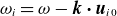 $\omega _i = \omega - \boldsymbol{k} \boldsymbol{\cdot }\boldsymbol{u}_{i0}$
, and assuming
$\omega _i = \omega - \boldsymbol{k} \boldsymbol{\cdot }\boldsymbol{u}_{i0}$
, and assuming
 $u_{iz0} \leq O(c_S)$
and
$u_{iz0} \leq O(c_S)$
and
 $|\omega _i| \sim |\omega | \geq O(k c_S) \gg O(\omega _{ci})$
, where
$|\omega _i| \sim |\omega | \geq O(k c_S) \gg O(\omega _{ci})$
, where
 $c_S = (T_{e0}/m_i)^{1/2}$
is the sound speed and
$c_S = (T_{e0}/m_i)^{1/2}$
is the sound speed and
 $\omega _{cs}= eB/m_s$
is the cyclotron frequency of species
$\omega _{cs}= eB/m_s$
is the cyclotron frequency of species
 $s$
, one obtains the relation between the density and electric potential perturbations (Esipchuk & Tilinin Reference Esipchuk and Tilinin1976; Frias et al. Reference Frias, Smolyakov, Kaganovich and Raitses2012; Smolyakov et al. Reference Smolyakov, Chapurin, Frias, Koshkarov, Romadanov, Tang, Umansky, Raitses, Kaganovich and Lakhin2017; Lakhin et al. Reference Lakhin, Ilgisonis, Smolyakov, Sorokina and Marusov2018; Ramos et al. Reference Ramos, Bello-Benítez and Ahedo2021; Ripoli et al. Reference Ripoli, Ahedo and Merino2025),
$s$
, one obtains the relation between the density and electric potential perturbations (Esipchuk & Tilinin Reference Esipchuk and Tilinin1976; Frias et al. Reference Frias, Smolyakov, Kaganovich and Raitses2012; Smolyakov et al. Reference Smolyakov, Chapurin, Frias, Koshkarov, Romadanov, Tang, Umansky, Raitses, Kaganovich and Lakhin2017; Lakhin et al. Reference Lakhin, Ilgisonis, Smolyakov, Sorokina and Marusov2018; Ramos et al. Reference Ramos, Bello-Benítez and Ahedo2021; Ripoli et al. Reference Ripoli, Ahedo and Merino2025),
 \begin{eqnarray} n_1 = \frac {e n_0 k^2}{m_i \omega _i^2} \ \phi _1 . \end{eqnarray}
2.2. Drift-kinetic electrons
For
 $|\omega | \ll \omega _{ce}$
,
$|\omega | \ll \omega _{ce}$
,
 $k \rho _e \ll 1$
and the assumed two-dimensional geometry with vanishing parallel gradients, the leading-order electron distribution function,
$k \rho _e \ll 1$
and the assumed two-dimensional geometry with vanishing parallel gradients, the leading-order electron distribution function,
 $f_e(w_\parallel , w_\perp , \boldsymbol{x}, t)$
, is independent of the gyrophase angle and satisfies the following collisionless drift-kinetic equation (Ramos Reference Ramos2008) in the reference frame of the macroscopic fluid velocity, i.e
$f_e(w_\parallel , w_\perp , \boldsymbol{x}, t)$
, is independent of the gyrophase angle and satisfies the following collisionless drift-kinetic equation (Ramos Reference Ramos2008) in the reference frame of the macroscopic fluid velocity, i.e
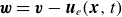 $\boldsymbol{w} = \boldsymbol{v} - \boldsymbol{u}_e(\boldsymbol{x},t)$
, where
$\boldsymbol{w} = \boldsymbol{v} - \boldsymbol{u}_e(\boldsymbol{x},t)$
, where
 $\boldsymbol{v}$
is the velocity coordinate in the laboratory frame:
$\boldsymbol{v}$
is the velocity coordinate in the laboratory frame:
 \begin{eqnarray} \frac {\partial f_e}{\partial t} + \left (\boldsymbol{u}_E - \frac {m_e w_\perp ^2}{2eB} \boldsymbol{e}_x\!\times\!\boldsymbol{\nabla }\ln B \right ) \boldsymbol{\cdot }\frac {\partial f_e}{\partial \boldsymbol{x}} - \frac {w_\perp }{2} \left (\boldsymbol{\nabla }\boldsymbol{\cdot }\boldsymbol{u}_E \right ) \frac {\partial f_e}{\partial w_\perp } = 0 . \end{eqnarray}
Here,
 $\boldsymbol{u}_E = B^{-1}\boldsymbol{e}_x\!\times\!\boldsymbol{\nabla }\phi$
is the electric drift velocity, so
$\boldsymbol{u}_E = B^{-1}\boldsymbol{e}_x\!\times\!\boldsymbol{\nabla }\phi$
is the electric drift velocity, so
 $\boldsymbol{\nabla }\boldsymbol{\cdot }\boldsymbol{ u}_E = B^{-1} \boldsymbol{e}_x \boldsymbol{\cdot }(\boldsymbol{\nabla }\ln B\!\times\!\boldsymbol{\nabla }\phi )$
. This applies to the lowest order in the small Larmor radius where the electron fluid velocity
$\boldsymbol{\nabla }\boldsymbol{\cdot }\boldsymbol{ u}_E = B^{-1} \boldsymbol{e}_x \boldsymbol{\cdot }(\boldsymbol{\nabla }\ln B\!\times\!\boldsymbol{\nabla }\phi )$
. This applies to the lowest order in the small Larmor radius where the electron fluid velocity
 $\boldsymbol{u}_e$
can be taken as the sum of the electric drift
$\boldsymbol{u}_e$
can be taken as the sum of the electric drift
 $\boldsymbol{u}_E$
plus a diamagnetic drift.
$\boldsymbol{u}_E$
plus a diamagnetic drift.
Linearising about a spatially one-dimensional equilibrium that depends on the
 $z$
-coordinate,
$z$
-coordinate,
 \begin{eqnarray} -i \omega f_{e1} \ & + & \ i k_y u_{E0} f_{e1} + \frac {ik_y}{B} \frac {\partial f_{e0}}{\partial z} \phi _1 + \frac {i k_y m_e w_\perp ^2}{2eB} \frac {\partial \ln B}{\partial z} f_{e1} \nonumber\\[4pt]& +& \ \frac {i k_y }{2B} \frac {\partial \ln B}{\partial z} w_\perp \frac {\partial f_{e0}}{\partial w_\perp } \phi _1 = 0 \end{eqnarray}
and, defining
 $\omega ' = \omega - k_y u_{E0}$
with
$\omega ' = \omega - k_y u_{E0}$
with
 $u_{E0} = - B^{-1} \partial \phi _0 / \partial z$
,
$u_{E0} = - B^{-1} \partial \phi _0 / \partial z$
,
 \begin{eqnarray} \left ( \omega ' - \frac {k_y m_e w_\perp ^2}{2eB} \frac {\partial \ln B}{\partial z} \right ) f_{e1} = \frac {k_y}{B} \left ( \frac {\partial f_{e0}}{\partial z} + \frac {1}{2} \frac {\partial \ln B}{\partial z} w_\perp \frac {\partial f_{e0}}{\partial w_\perp } \right ) \phi _1 . \end{eqnarray}
Assuming a Maxwellian equilibrium distribution function,
 \begin{eqnarray} f_{e0} = n_0 \left (\frac {m_e}{2\pi T_{e0}}\right )^{3/2} \exp \left (-\frac {m_e w^2}{2 T_{e0}} \right )\!, \end{eqnarray}
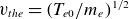
with the thermal velocity defined as
 $v_{the} = (T_{e0}/m_e)^{1/2}$
, and introducing the definitions
$v_{the} = (T_{e0}/m_e)^{1/2}$
, and introducing the definitions
 \begin{eqnarray} \omega _{*N} = - k_y \frac {T_{e0}}{eB} \ \frac {\partial \ln n_0}{\partial z} , \quad \omega _{*T} = - k_y \frac {T_{e0}}{eB} \ \frac {\partial \ln T_{e0}}{\partial z} , \quad \omega _{*B} = - k_y \frac {T_{e0}}{eB} \ \frac {\partial \ln B}{\partial z} , \qquad \end{eqnarray}
one obtains
 \begin{eqnarray} \left ( \omega ' + \frac {w_\perp ^2}{2 v_{the}^2} \omega _{*B} \right ) f_{e1} & = & - \ \frac {e n_0 \phi _1}{(2 \pi )^{3/2} T_{e0} v_{the}^3} \left [ \omega _{*N} + \left (\frac {w^2}{2 v_{the}^2} - \frac {3}{2} \right ) \omega _{*T} - \frac {w_\perp ^2}{2 v_{the}^2} \omega _{*B} \right ] \nonumber\\[12pt]&& \quad\times \exp \left ( - \frac {w^2}{2 v_{the}^2} \right )\!. \end{eqnarray}
The perturbed electron density is
 \begin{align} n_1 = 2 \pi \int_{- \infty }^\infty \text{d} w_\parallel \int _0^\infty \text{d} w_\perp \ w_\perp \ f_{e1} \end{align}
and, substituting the solution (2.11) for
 $f_{e1}$
,
$f_{e1}$
,
 \begin{align} n_1 &= - \ \frac{e n_0 \phi_1}{(2 \pi)^{1/2} T_{e0} v_{the}^3} \int_{- \infty}^\infty \textrm{d} w_\parallel \int_0^\infty \textrm{d} w_\perp \ w_\perp \ \nonumber \\& \quad \times \frac{\omega_{*N} + \left({w^2}/{2 v_{the}^2} - {3}/{2} \right) \omega_{*T} - ({w_\perp^2}/{2 v_{the}^2}) \omega_{*B}}{\omega' + ({w_\perp^2}/{2 v_{the}^2}) \omega_{*B}} \exp \left( - \frac{w^2}{2 v_{the}^2} \right)\!. \end{align}
Finally, carrying out the integral over
 $w_\parallel$
and calling
$w_\parallel$
and calling
 $s=w_\perp ^2 / (2 v_{the}^2)$
,
$s=w_\perp ^2 / (2 v_{the}^2)$
,
 \begin{eqnarray} n_1 = - \ \frac {e n_0 \phi _1}{T_{e0}} \int _0^\infty \,\mathrm{d}s \ \frac {\omega _{*N} + \omega _{*T} (s-1) - \omega _{*B} \ s}{\omega ' + \omega _{*B} \ s} \ \exp (-s), \end{eqnarray}
defined for those values of the plasma parameters and the mode frequency such that the integrand does not diverge on the integration path
 $(0 \lt s \lt \infty )$
and the integral exists.
$(0 \lt s \lt \infty )$
and the integral exists.
3. Dispersion relation for an homogeneous magnetic field
In the special case of an homogeneous magnetic field,
 $\omega _{*B}=0$
and the integral of (2.14) is elementary, yielding
$\omega _{*B}=0$
and the integral of (2.14) is elementary, yielding
 \begin{eqnarray} n_1 = - \ \frac {e n_0 \phi _1}{T_{e0}} \ \frac {\omega _{*N}}{\omega '} . \end{eqnarray}
Notice that the contribution of
 $\omega _{*T}$
cancels out. This result coincides with the familiar one derived from fluid theory in the lowest order of the small electron Larmor radius where the electron inertia and gyroviscosity can be neglected in the momentum equation. In this limit, the electron fluid system reduces to
$\omega _{*T}$
cancels out. This result coincides with the familiar one derived from fluid theory in the lowest order of the small electron Larmor radius where the electron inertia and gyroviscosity can be neglected in the momentum equation. In this limit, the electron fluid system reduces to
 \begin{eqnarray} \frac {\partial n}{\partial t} + \boldsymbol{\nabla }\boldsymbol{\cdot }(n \boldsymbol{u}_e) = 0 , \end{eqnarray}
 \begin{eqnarray} \boldsymbol{\nabla }p_e + e n \left (- \boldsymbol{\nabla }\phi + B \boldsymbol{u}_e\!\times\!\boldsymbol{e}_x \right ) = 0 . \end{eqnarray}
Solving for the electron current,
 \begin{eqnarray} n \boldsymbol{u}_e = \frac {1}{eB} \ \boldsymbol{e}_x \times \left (en \boldsymbol{\nabla }\phi - \boldsymbol{\nabla }p_e \right ) \end{eqnarray}
and, taking into account that here
 $B$
is constant,
$B$
is constant,
 \begin{eqnarray} \boldsymbol{\nabla }\boldsymbol{\cdot }(n \boldsymbol{u}_e) = \frac {1}{B} \ \boldsymbol{e}_x \boldsymbol{\cdot }\left ( \boldsymbol{\nabla }\phi\!\times\!\boldsymbol{\nabla }n \right)\!. \end{eqnarray}
Bringing this to the continuity equation and linearising, one gets
 \begin{eqnarray} (\omega - k_y u_{E0}) n_1 + \frac {e n_0 \omega _{*N}}{T_{e0}} \phi _1 = 0 , \end{eqnarray}
which is the same as (3.1).
Combining (2.5) and (3.1), one obtains the dispersion relation for an homogeneous magnetic field (Smolyakov et al. Reference Smolyakov, Chapurin, Frias, Koshkarov, Romadanov, Tang, Umansky, Raitses, Kaganovich and Lakhin2017)
 \begin{eqnarray} \omega _{*N} \ \omega _i^2 + k^2 c_S^2 (\omega _i - {\hat \varDelta }) = 0 , \end{eqnarray}
where
 \begin{eqnarray} {\hat \varDelta } = \omega _i - \omega ' = k_y u_{E0} - \boldsymbol{k} \boldsymbol{\cdot }\boldsymbol{u}_{i0} . \end{eqnarray}
This quadratic dispersion relation has an unstable complex root for
 \begin{eqnarray} {\hat \varDelta } \ \omega _{*N} \lt \frac{- k^2 c_S^2}{4}, \end{eqnarray}
which is the criterion for the (collisionless) S–H instability, including in
 $\hat \varDelta$
the ion-drift effect (Sakawa et al. Reference Sakawa, Joshi, Kaw, Chen and Jain1993). So, in the two-dimensional theory being considered here with
$\hat \varDelta$
the ion-drift effect (Sakawa et al. Reference Sakawa, Joshi, Kaw, Chen and Jain1993). So, in the two-dimensional theory being considered here with
 $k_\parallel =0$
, there is no kinetic effect on the low-frequency dispersion relation if the magnetic field is homogeneous, the only instability being the fluid drift-gradient mode driven by the equilibrium density gradient. To have an instability driven by the temperature gradient, a non-zero gradient of the magnetic field is necessary.
$k_\parallel =0$
, there is no kinetic effect on the low-frequency dispersion relation if the magnetic field is homogeneous, the only instability being the fluid drift-gradient mode driven by the equilibrium density gradient. To have an instability driven by the temperature gradient, a non-zero gradient of the magnetic field is necessary.
4. Dispersion relation for an inhomogeneous magnetic field
For
 $\omega _{*B} \not = 0$
, calling
$\omega _{*B} \not = 0$
, calling
 $\zeta = \omega ' / \omega _{*B}$
, (2.14) can be rewritten as
$\zeta = \omega ' / \omega _{*B}$
, (2.14) can be rewritten as
 \begin{eqnarray} n_1 = \frac {e n_0 \phi _1}{T_{e0} \ \omega _{*B}} \left[(\omega _{*T} - \omega _{*N}) \ g(\zeta ) - (\omega _{*T} - \omega _{*B}) \ h(\zeta ) \right] , \end{eqnarray}
where
 \begin{eqnarray} g(\zeta ) = \int _0^\infty\, \text{d}s \ \frac {\exp (-s)}{\zeta + s} \end{eqnarray}
and
 \begin{eqnarray} h(\zeta ) = \int _0^\infty \,\text{d}s \ \frac {s \ \exp (-s)}{\zeta + s} = 1 - \zeta \ g(\zeta ) . \end{eqnarray}
The function
 $g(\zeta )$
is real analytic, i.e.
$g(\zeta )$
is real analytic, i.e.
 $g(\zeta ^*) = g(\zeta )^*$
, and it has a branch cut for real and negative
$g(\zeta ^*) = g(\zeta )^*$
, and it has a branch cut for real and negative
 $\zeta$
with logarithmic singularities at
$\zeta$
with logarithmic singularities at
 $\zeta =0$
and at infinity. It is related to the exponential integral function (Abramowitz & Stegun Reference Abramowitz and Stegun1965)
$\zeta =0$
and at infinity. It is related to the exponential integral function (Abramowitz & Stegun Reference Abramowitz and Stegun1965)
 $E_1(\zeta )$
through
$E_1(\zeta )$
through
 \begin{eqnarray} g(\zeta ) = \exp (\zeta ) \ E_1(\zeta ), \end{eqnarray}
where
 \begin{eqnarray} E_1(\zeta ) = \int _\zeta ^\infty \,\text{d} \sigma \ \frac {\exp (-\sigma )}{\sigma } = - \left [\ln \zeta + \gamma + \sum _{m=1}^\infty \frac {(-1)^m \zeta ^m}{m \ m!} \right ] \end{eqnarray}
and
 $\gamma$
is the Euler–Mascheroni constant. The derivative of
$\gamma$
is the Euler–Mascheroni constant. The derivative of
 $g(\zeta )$
is defined everywhere except at its singular half-line,
$g(\zeta )$
is defined everywhere except at its singular half-line,
 \begin{eqnarray} \frac {\text{d} g(\zeta )}{\text{d} \zeta } = g(\zeta ) - \frac {1}{\zeta } . \end{eqnarray}
Taking successive derivatives, we obtain
 \begin{eqnarray} g(\zeta ) = \frac {1}{\zeta } - \frac {1}{\zeta ^2} + \frac {2}{\zeta ^3} - \frac {3!}{\zeta ^4} + \cdots + \frac {(-1)^k k!}{\zeta ^{k+1}} + \frac {\text{d}^{k+1} g(\zeta )}{\text{d} \zeta ^{k+1}}, \end{eqnarray}
which applies where the derivatives of
 $g(\zeta )$
exist, i.e. everywhere except for real non-positive
$g(\zeta )$
exist, i.e. everywhere except for real non-positive
 $\zeta$
. Disregarding the residual term
$\zeta$
. Disregarding the residual term
 $d^{k+1} g(\zeta )/d \zeta ^{k+1} = O(1/|\zeta |^{k+2})$
and letting
$d^{k+1} g(\zeta )/d \zeta ^{k+1} = O(1/|\zeta |^{k+2})$
and letting
 $k$
go to infinity, (4.7) can be considered as a power expansion of
$k$
go to infinity, (4.7) can be considered as a power expansion of
 $g(\zeta )$
for large argument. However, this is only a non-converging asymptotic series, so care must be exercised when using it. Most crucially, it does not reproduce the singular behaviour of
$g(\zeta )$
for large argument. However, this is only a non-converging asymptotic series, so care must be exercised when using it. Most crucially, it does not reproduce the singular behaviour of
 $g(\zeta )$
as
$g(\zeta )$
as
 $\zeta$
approaches a real and negative value, whose physical origin is the resonant character of the kinetic perturbation of the electron distribution function (2.13). This issue is dealt with in more detail in Appendix B, where an exponentially small correction is added in the case of
$\zeta$
approaches a real and negative value, whose physical origin is the resonant character of the kinetic perturbation of the electron distribution function (2.13). This issue is dealt with in more detail in Appendix B, where an exponentially small correction is added in the case of
 $\zeta$
being close to real and negative, which recovers faithfully that singularity.
$\zeta$
being close to real and negative, which recovers faithfully that singularity.
In terms of
 $\zeta$
, (2.5) can be rewritten as
$\zeta$
, (2.5) can be rewritten as
 \begin{eqnarray} n_1 = \frac {e n_0 k^2}{m_i \omega _{*B}^2 (\zeta + {\hat \varDelta } / \omega _{*B})^2} \ \phi _1 \end{eqnarray}
and, combining (4.1), (4.3) and (4.8), we obtain the final dispersion relation
 \begin{eqnarray} \frac {k^2 c_S^2}{(\zeta + {\hat \varDelta } / \omega _{*B})^2} = \omega _{*B}\{[(\omega _{*T} - \omega _{*N}) + (\omega _{*T} - \omega _{*B}) \zeta] g(\zeta ) - (\omega _{*T} - \omega _{*B}) \} .\qquad \end{eqnarray}
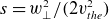
So, defining the three real dimensionless parameters,
 \begin{eqnarray} \alpha = \frac {\omega _{*B}(\omega _{*N} - \omega _{*B})}{k^2 c_S^2} , \ \beta = \frac {\omega _{*B}(\omega _{*T} - \omega _{*B})}{k^2 c_S^2} , \ \delta = \frac {{\hat \varDelta }}{\omega _{*B}} = \frac {k_y u_{E0} - \boldsymbol{k} \boldsymbol{\cdot }\boldsymbol{u}_{i0}}{\omega _{*B}} ,\qquad \end{eqnarray}
the dimensionless form of the dispersion relation is
 \begin{eqnarray} \frac {1}{(\zeta + \delta )^2} + [\alpha - \beta (1+\zeta )] \ g(\zeta ) + \beta = 0 , \end{eqnarray}
whose roots are either real roots or complex conjugate pairs, since
 $g(\zeta )$
is real analytic. Notice that the dimensionless variables in (4.11) are independent of the magnitude
$g(\zeta )$
is real analytic. Notice that the dimensionless variables in (4.11) are independent of the magnitude
 $k$
of the wavevector,
$k$
of the wavevector,
 $\boldsymbol{k} = k_y\boldsymbol{e}_y + k_z\boldsymbol{e}_z = k(\cos \theta \boldsymbol{e}_y +\sin \theta \boldsymbol{e}_z)$
, and depend only on the propagation angle
$\boldsymbol{k} = k_y\boldsymbol{e}_y + k_z\boldsymbol{e}_z = k(\cos \theta \boldsymbol{e}_y +\sin \theta \boldsymbol{e}_z)$
, and depend only on the propagation angle
 $\theta$
. As a consequence of this and the definition of
$\theta$
. As a consequence of this and the definition of
 $\zeta = \omega ' / \omega _{*B}$
, the dimensional complex frequency
$\zeta = \omega ' / \omega _{*B}$
, the dimensional complex frequency
 $\omega$
scales proportional to
$\omega$
scales proportional to
 $k$
in the long-wavelength regime
$k$
in the long-wavelength regime
 $k \rho _e \ll 1$
that this work considers.
$k \rho _e \ll 1$
that this work considers.
5. Parametric range of instability
The dispersion relation for an inhomogeneous magnetic field, (4.9) or (4.11), is a transcendental equation whose normalised frequency roots have to be found numerically. However, the marginal stability boundary in parameter space between the region where it has complex roots (i.e. where the plasma equilibrium is unstable) and the region where it does not have any complex root (i.e. where the plasma equilibrium is stable) can be found analytically. The detailed mathematical derivation of those marginal stability conditions is given in Appendices A and B.
Parametric range of instability from the kinetic dispersion relation (4.11) in the
 $(\alpha$
,
$(\alpha$
,
 $\beta )$
plane for several representative values of
$\beta )$
plane for several representative values of
 $\delta$
. The white region is stable, while a colour scale indicates the normalised instability growth rate in the unstable region. The green, blue and red solid lines represent the marginal stability boundaries obtained analytically.
$\delta$
. The white region is stable, while a colour scale indicates the normalised instability growth rate in the unstable region. The green, blue and red solid lines represent the marginal stability boundaries obtained analytically.

Figure 1 displays the analytic instability thresholds (shown as green, blue and red solid lines) and the regions of instability (indicated with a colour scale that represents the numerical growth rates) in
 $(\alpha , \beta )$
parametric planes at constant
$(\alpha , \beta )$
parametric planes at constant
 $\delta$
for six representative values of the latter. The agreement between the analytic and numerical results is excellent. The marginal stability boundary is divided in three sections. The lines coloured green correspond to a resonant instability threshold, where a pair of complex conjugate roots of the dispersion relation emerges at its logarithmic branch cut, with a marginal normalised real frequency
$\delta$
for six representative values of the latter. The agreement between the analytic and numerical results is excellent. The marginal stability boundary is divided in three sections. The lines coloured green correspond to a resonant instability threshold, where a pair of complex conjugate roots of the dispersion relation emerges at its logarithmic branch cut, with a marginal normalised real frequency
 $\zeta$
negative. This resonant instability threshold is given by the conditions
$\zeta$
negative. This resonant instability threshold is given by the conditions
 $\beta \leq 0$
,
$\beta \leq 0$
,
 $\beta \leq \alpha$
and
$\beta \leq \alpha$
and
 $\alpha = \beta (1-\delta ) \pm \sqrt {-\beta }$
. It connects the point
$\alpha = \beta (1-\delta ) \pm \sqrt {-\beta }$
. It connects the point
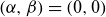 $(\alpha , \beta )=(0,0)$
where
$(\alpha , \beta )=(0,0)$
where
 $\zeta \rightarrow - \infty$
, with the point
$\zeta \rightarrow - \infty$
, with the point
 $(\alpha , \beta )=(-\delta ^{-2}, -\delta ^{-2})$
where
$(\alpha , \beta )=(-\delta ^{-2}, -\delta ^{-2})$
where
 $\zeta \rightarrow 0_{-}$
. The connecting path is continuous if
$\zeta \rightarrow 0_{-}$
. The connecting path is continuous if
 $\delta \lt 0$
, whereas it goes through infinity if
$\delta \lt 0$
, whereas it goes through infinity if
 $\delta \geq 0$
. The lines coloured blue correspond to a non-resonant or fluid-like instability threshold, where a pair of complex conjugate roots of the dispersion relation evolves from a pair of real roots that coalesce into a double root, with a marginal normalised real frequency
$\delta \geq 0$
. The lines coloured blue correspond to a non-resonant or fluid-like instability threshold, where a pair of complex conjugate roots of the dispersion relation evolves from a pair of real roots that coalesce into a double root, with a marginal normalised real frequency
 $\zeta$
positive. The equation for this non-resonant instability threshold is given in parametric form by (A12) and (A13). It connects the point
$\zeta$
positive. The equation for this non-resonant instability threshold is given in parametric form by (A12) and (A13). It connects the point
 $(\alpha , \beta )=(-\delta ^{-2}, -\delta ^{-2})$
where
$(\alpha , \beta )=(-\delta ^{-2}, -\delta ^{-2})$
where
 $\zeta \rightarrow 0_{+}$
with the point
$\zeta \rightarrow 0_{+}$
with the point
 $(\alpha , \beta )=(0,1)$
where
$(\alpha , \beta )=(0,1)$
where
 $\zeta \rightarrow + \infty$
. This connecting path is continuous if
$\zeta \rightarrow + \infty$
. This connecting path is continuous if
 $\delta \gt 0$
, whereas it goes through infinity if
$\delta \gt 0$
, whereas it goes through infinity if
 $\delta \leq 0$
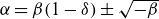
. Finally, the segment
$\delta \leq 0$
. Finally, the segment
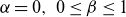 $\alpha =0, \ 0 \leq \beta \leq 1$
, coloured red, corresponds to a resonant instability threshold where a pair of complex conjugate roots of the dispersion relation emerges at infinity. On the stable
$\alpha =0, \ 0 \leq \beta \leq 1$
, coloured red, corresponds to a resonant instability threshold where a pair of complex conjugate roots of the dispersion relation emerges at infinity. On the stable
 $\alpha \lt 0$
side, there is a large positive real root, while on the unstable
$\alpha \lt 0$
side, there is a large positive real root, while on the unstable
 $\alpha \gt 0$
side, a complex pair appears with large negative real part and exponentially small imaginary part.
$\alpha \gt 0$
side, a complex pair appears with large negative real part and exponentially small imaginary part.
Figure 2 displays the same information, in
 $(\alpha , \delta )$
parametric planes at constant
$(\alpha , \delta )$
parametric planes at constant
 $\beta$
. For
$\beta$
. For
 $\beta \gt 1$
, all the instability thresholds are of the non-resonant type. For
$\beta \gt 1$
, all the instability thresholds are of the non-resonant type. For
 $0 \leq \beta \leq 1$
, we have non-resonant and root-at-infinity thresholds. For
$0 \leq \beta \leq 1$
, we have non-resonant and root-at-infinity thresholds. For
 $\beta \lt 0$
, we have both the non-resonant and the resonant with root at the branch cut types of thresholds, the latter appearing now as two parallel straight half-lines that leave a stable band in between. These two parallel lines start at the points
$\beta \lt 0$
, we have both the non-resonant and the resonant with root at the branch cut types of thresholds, the latter appearing now as two parallel straight half-lines that leave a stable band in between. These two parallel lines start at the points
 $(\alpha , \delta ) = (\beta , \pm 1/\sqrt {-\beta })$
and have slope
$(\alpha , \delta ) = (\beta , \pm 1/\sqrt {-\beta })$
and have slope
 $-1/\beta$
, so the width of the stable band shrinks to zero both as
$-1/\beta$
, so the width of the stable band shrinks to zero both as
 $\beta \rightarrow 0_-$
when the lines merge with the
$\beta \rightarrow 0_-$
when the lines merge with the
 $\alpha =0$
axis and as
$\alpha =0$
axis and as
 $\beta \rightarrow -\infty$
when the lines merge with the
$\beta \rightarrow -\infty$
when the lines merge with the
 $\delta = 0$
axis.
$\delta = 0$
axis.
Parametric range of instability from the kinetic dispersion relation (4.11) in the
 $(\alpha$
,
$(\alpha$
,
 $\delta )$
plane for several representative values of
$\delta )$
plane for several representative values of
 $\beta$
. The white region is stable, while a colour scale indicates the normalised instability growth rate in the unstable region. The green, blue and red solid lines represent the marginal stability boundaries obtained analytically.
$\beta$
. The white region is stable, while a colour scale indicates the normalised instability growth rate in the unstable region. The green, blue and red solid lines represent the marginal stability boundaries obtained analytically.

In these
 $(\alpha , \delta )$
planes, we see that the instability largely fills the first, second and fourth quadrants. The third quadrant is stable for positive
$(\alpha , \delta )$
planes, we see that the instability largely fills the first, second and fourth quadrants. The third quadrant is stable for positive
 $\beta$
, but develops an increasingly large region of instability as
$\beta$
, but develops an increasingly large region of instability as
 $\beta$
becomes increasingly negative. Recalling the definitions (2.10) and (4.10),
$\beta$
becomes increasingly negative. Recalling the definitions (2.10) and (4.10),
 $\alpha$
and
$\alpha$
and
 $\beta$
are positive when the gradients of
$\beta$
are positive when the gradients of
 $n_0/B$
and
$n_0/B$
and
 $T_{e0}/B$
, respectively, point in the direction of the gradient of
$T_{e0}/B$
, respectively, point in the direction of the gradient of
 $B$
. Also, if we assume for simplicity
$B$
. Also, if we assume for simplicity
 $|k_y u_{E0}| \gg |\boldsymbol{k} \boldsymbol{\cdot }\boldsymbol{u}_{i0}|$
as is often the case,
$|k_y u_{E0}| \gg |\boldsymbol{k} \boldsymbol{\cdot }\boldsymbol{u}_{i0}|$
as is often the case,
 $\delta$
is positive when the applied equilibrium electric field points opposite to the direction of the gradient of
$\delta$
is positive when the applied equilibrium electric field points opposite to the direction of the gradient of
 $B$
. Therefore, the second and fourth quadrants,
$B$
. Therefore, the second and fourth quadrants,
 $\alpha \delta \lt 0$
, correspond to the gradient of
$\alpha \delta \lt 0$
, correspond to the gradient of
 $n_0/B$
pointing in the direction of the applied electric field, which is the condition for the classic Simon–Hoh instability. Accordingly, we may regard the instability in those second and fourth quadrants as a generalisation of the S–H instability, now modified in a kinetically consistent manner by the effects of the gradients of the magnetic field and the electron temperature. These kinetic modifications are significant and the classic form of the S–H instability threshold in (3.9),
$n_0/B$
pointing in the direction of the applied electric field, which is the condition for the classic Simon–Hoh instability. Accordingly, we may regard the instability in those second and fourth quadrants as a generalisation of the S–H instability, now modified in a kinetically consistent manner by the effects of the gradients of the magnetic field and the electron temperature. These kinetic modifications are significant and the classic form of the S–H instability threshold in (3.9),
 $\alpha \delta \simeq -1/4$
, is observed only in the narrow parametric region characterised by
$\alpha \delta \simeq -1/4$
, is observed only in the narrow parametric region characterised by
 $|\beta | \ll 1, \ |\alpha | \sim |\delta |^{-1} \ll 1$
and
$|\beta | \ll 1, \ |\alpha | \sim |\delta |^{-1} \ll 1$
and
 $\alpha \lt 0$
that will be studied in the next section.
$\alpha \lt 0$
that will be studied in the next section.
The instability in the first and third quadrants is unconventional, as it happens when the gradient of
 $n_0/B$
points opposite to the applied electric field. This instability, not of S–H character, becomes generally stronger as the magnitude of
$n_0/B$
points opposite to the applied electric field. This instability, not of S–H character, becomes generally stronger as the magnitude of
 $\beta$
increases, indicating a drive due to the electron temperature gradient. In the first quadrant, where the gradient of
$\beta$
increases, indicating a drive due to the electron temperature gradient. In the first quadrant, where the gradient of
 $n_0/B$
is in the direction of the gradient of
$n_0/B$
is in the direction of the gradient of
 $B$
, we observe a relatively weak resonant instability with a stable band if
$B$
, we observe a relatively weak resonant instability with a stable band if
 $\beta \lt 0$
(i.e. if the gradient of
$\beta \lt 0$
(i.e. if the gradient of
 $T_{e0}/B$
is opposite to the gradients of
$T_{e0}/B$
is opposite to the gradients of
 $n_0/B$
and
$n_0/B$
and
 $B$
), but a more robust instability if
$B$
), but a more robust instability if
 $\beta$
is positive and increasing (i.e. if the gradient of
$\beta$
is positive and increasing (i.e. if the gradient of
 $T_{e0}/B$
is increasingly large in the direction of the gradients of
$T_{e0}/B$
is increasingly large in the direction of the gradients of
 $n_0/B$
and
$n_0/B$
and
 $B$
). The third quadrant, where the gradient of
$B$
). The third quadrant, where the gradient of
 $n_0/B$
is opposite to the gradient of
$n_0/B$
is opposite to the gradient of
 $B$
, is stable if
$B$
, is stable if
 $\beta \gt 0$
(i.e. if the gradient of
$\beta \gt 0$
(i.e. if the gradient of
 $T_{e0}/B$
is opposite to the gradient of
$T_{e0}/B$
is opposite to the gradient of
 $n_0/B$
). However, a strong non-resonant instability, clearly driven by the temperature gradient, appears in the third quadrant if
$n_0/B$
). However, a strong non-resonant instability, clearly driven by the temperature gradient, appears in the third quadrant if
 $\beta \lt 0$
(i.e. if the gradient of
$\beta \lt 0$
(i.e. if the gradient of
 $T_{e0}/B$
is in the direction of the gradient of
$T_{e0}/B$
is in the direction of the gradient of
 $n_0/B$
), with a condition for instability of the form
$n_0/B$
), with a condition for instability of the form
 $\beta \lt \beta _c(\alpha , \delta ) \lt 0$
. In summary, a robust instability, not of S–H character since it happens in the first or third quadrant where the gradient of
$\beta \lt \beta _c(\alpha , \delta ) \lt 0$
. In summary, a robust instability, not of S–H character since it happens in the first or third quadrant where the gradient of
 $n_0/B$
points opposite to the applied electric field, is observed when the gradient of
$n_0/B$
points opposite to the applied electric field, is observed when the gradient of
 $T_{e0}/B$
is in the direction of the gradient of
$T_{e0}/B$
is in the direction of the gradient of
 $n_0/B$
. It is triggered or becomes stronger as the magnitude of the electron temperature gradient increases, so it can be categorised as a type of ETG mode.
$n_0/B$
. It is triggered or becomes stronger as the magnitude of the electron temperature gradient increases, so it can be categorised as a type of ETG mode.
6. Weak magnetic inhomogeneity and comparison with the Simon–Hoh instability criterion
The kinetic analysis of §§ 4 and 5 necessitates a non-zero gradient of the magnetic field. This gives rise to a resonant contribution to the perturbation of the electron density in (2.14) that, for a weak magnetic gradient, comes from particles of high perpendicular velocity whose number is exponentially small, at the tail of their distribution function. Nevertheless, even if its quantitative effect may be small, the kinetic resonance is present no matter how small the magnetic gradient is, meaning a qualitative difference with the situation where the magnetic field is strictly constant and the resonance does not exist. Therefore, the approach, as the magnetic gradient tends to zero, of the kinetic result of §§ 4 and 5 towards the constant magnetic field result of § 3 (i.e. towards the classic S–H instability) is a non-trivial issue worth studying.
To investigate this, we consider a regime of weak magnetic inhomogeneity characterised by a magnetic gradient scale length
 $L_B = |\partial \ln B / \partial z|^{-1}$
much larger than the ion sound gyroradius
$L_B = |\partial \ln B / \partial z|^{-1}$
much larger than the ion sound gyroradius
 $\rho _S = c_S / \omega _{ci}$
. Thus, we introduce the small expansion parameter
$\rho _S = c_S / \omega _{ci}$
. Thus, we introduce the small expansion parameter
 \begin{eqnarray} \varepsilon = \frac {|\omega _{*B}|}{kc_S} = \frac {|k_y| \rho _S}{k L_B} \ll 1 . \end{eqnarray}
In addition, we assume the maximal ordering for the other variables,
 \begin{eqnarray} |\omega _{*N}| \sim |\omega _{*T}| \sim |{\hat \varDelta }| \sim |\omega '| \sim k c_S , \end{eqnarray}
which implies
 $|\alpha | \sim |\beta | \sim \varepsilon$
and
$|\alpha | \sim |\beta | \sim \varepsilon$
and
 $|\delta | \sim |\zeta | \sim \varepsilon ^{-1}$
. Then, we use the large-argument asymptotic expansion (4.7) to approximate the function
$|\delta | \sim |\zeta | \sim \varepsilon ^{-1}$
. Then, we use the large-argument asymptotic expansion (4.7) to approximate the function
 $g(\zeta )$
. Keeping the first two significant orders, our kinetic dispersion relation (4.11) reduces to
$g(\zeta )$
. Keeping the first two significant orders, our kinetic dispersion relation (4.11) reduces to
 \begin{eqnarray} (\zeta + \delta )^{-2} + \alpha (\zeta ^{-1} - \zeta ^{-2}) - \beta \ \zeta ^{-2} = O(|\alpha \zeta |^{-3}) + O(|\beta \zeta |^{-3}), \end{eqnarray}
or, equivalently,
 \begin{eqnarray} \alpha (\zeta + \delta )^2 + \zeta - (\alpha + \beta ) (\zeta + \delta )^2 \zeta ^{-1} = O(\varepsilon ) . \end{eqnarray}
This is a cubic equation for
 $\zeta$
that can be solved perturbatively. As a first approximation, we equate to zero the leading terms of this equation, which are its first two terms of order
$\zeta$
that can be solved perturbatively. As a first approximation, we equate to zero the leading terms of this equation, which are its first two terms of order
 $\varepsilon ^{-1}$
, to get the leading-order solution
$\varepsilon ^{-1}$
, to get the leading-order solution
 \begin{eqnarray} \zeta _0 = \frac {1}{2\alpha } \big[\!-(1+ 2 \alpha \delta ) \pm \sqrt {1+4 \alpha \delta } \big] . \end{eqnarray}
Then, we solve
 \begin{eqnarray} \alpha (\zeta + \delta )^2 + \zeta - (\alpha + \beta )(\zeta _0 + \delta )^2 \zeta _0^{-1} = 0 , \end{eqnarray}
which simplifies to
 \begin{eqnarray} \alpha (\zeta + \delta )^2 + \zeta + (\alpha + \beta ) / \alpha = 0 \end{eqnarray}
and yields
 \begin{eqnarray} \zeta = \frac {1}{2\alpha } \big[\!-(1+ 2 \alpha \delta ) \pm \sqrt {1+4 (\alpha \delta - \alpha - \beta )} \big] . \end{eqnarray}
This gives the condition for instability
 \begin{eqnarray} \alpha (\delta - 1) - \beta \lt - 1/4 \end{eqnarray}
or, in terms of dimensional parameters,
 \begin{eqnarray} ({\hat \varDelta } - \omega _{*B}) \ (\omega _{*N} - \omega _{*B}) - \omega _{*B} \ (\omega _{*T} - \omega _{*B}) \lt - k^2 c_S^2/4 . \end{eqnarray}
For the unstable range of these parameters, the growth rate of the instability is
 \begin{align} {\rm Im} \omega = \frac {k c_S}{|\omega _{*N} - \omega _{*B}|} \bigl [\omega _{*B} \ (\omega _{*T} - \omega _{*B})-({\hat \varDelta } - \omega _{*B}) \ (\omega _{*N} - \omega _{*B}) - k^2 c_S^2/4 \bigr ]^{1/2} . \end{align}
In the limit
 $\omega _{*B} \rightarrow 0$
, (6.10) becomes the same as (3.9) and the growth rate (6.11) becomes the same as the corresponding growth rate of order
$\omega _{*B} \rightarrow 0$
, (6.10) becomes the same as (3.9) and the growth rate (6.11) becomes the same as the corresponding growth rate of order
 $kc_S$
, so our kinetic theory recovers the S–H instability criterion for an homogeneous magnetic field. Moreover, (6.10) and (6.11) provide a kinetically based extension of such a criterion that includes the gradients of the magnetic field and the electron temperature, albeit in a perturbative sense for small
$kc_S$
, so our kinetic theory recovers the S–H instability criterion for an homogeneous magnetic field. Moreover, (6.10) and (6.11) provide a kinetically based extension of such a criterion that includes the gradients of the magnetic field and the electron temperature, albeit in a perturbative sense for small
 $\omega _{*B} / k \rho _S$
. This kinetically based extension should be contrasted with other extensions of the S–H criterion (Frias et al. Reference Frias, Smolyakov, Kaganovich and Raitses2012; Smolyakov et al. Reference Smolyakov, Chapurin, Frias, Koshkarov, Romadanov, Tang, Umansky, Raitses, Kaganovich and Lakhin2017; Ramos et al. Reference Ramos, Bello-Benítez and Ahedo2021; Boeuf & Smolyakov Reference Boeuf and Smolyakov2023; Ripoli et al. Reference Ripoli, Ahedo and Merino2025) derived within the fluid theory framework under various working hypotheses.
$\omega _{*B} / k \rho _S$
. This kinetically based extension should be contrasted with other extensions of the S–H criterion (Frias et al. Reference Frias, Smolyakov, Kaganovich and Raitses2012; Smolyakov et al. Reference Smolyakov, Chapurin, Frias, Koshkarov, Romadanov, Tang, Umansky, Raitses, Kaganovich and Lakhin2017; Ramos et al. Reference Ramos, Bello-Benítez and Ahedo2021; Boeuf & Smolyakov Reference Boeuf and Smolyakov2023; Ripoli et al. Reference Ripoli, Ahedo and Merino2025) derived within the fluid theory framework under various working hypotheses.
The regime of weak magnetic inhomogeneity under consideration has another region of instability in the parametric domain characterised by the alternative orderings
 \begin{eqnarray} |\omega _{*N}| \sim \varepsilon ^{1/2} kc_S , \qquad |\omega _{*T}| \sim |{\hat \varDelta }| \sim k c_S , \end{eqnarray}
where a frequency solution of the order
 $|\omega '| \sim \varepsilon ^{1/2} kc_S$
is found. This implies
$|\omega '| \sim \varepsilon ^{1/2} kc_S$
is found. This implies
 $|\alpha | \sim \varepsilon ^{3/2}, \ |\beta | \sim \varepsilon , \ |\delta | \sim \varepsilon ^{-1}$
and
$|\alpha | \sim \varepsilon ^{3/2}, \ |\beta | \sim \varepsilon , \ |\delta | \sim \varepsilon ^{-1}$
and
 $|\zeta | \sim \varepsilon ^{-1/2}$
, so the large-argument approximation for
$|\zeta | \sim \varepsilon ^{-1/2}$
, so the large-argument approximation for
 $g(\zeta )$
can still be used. Bringing these alternative orderings to (6.4), the leading terms are now of order
$g(\zeta )$
can still be used. Bringing these alternative orderings to (6.4), the leading terms are now of order
 $\varepsilon ^{-1/2}$
and give
$\varepsilon ^{-1/2}$
and give
 \begin{eqnarray} \alpha \delta ^2 + \zeta - \beta \delta ^2 \zeta ^{-1} = 0 \,. \end{eqnarray}
This has the solution
 \begin{align} \zeta = \frac {1}{2} \Bigl (-\alpha \delta ^2 \pm \delta \sqrt {\alpha ^2 \delta ^2 + 4 \beta } \Bigr ), \end{align}
with the condition for instability
 \begin{eqnarray} \beta \lt - \alpha ^2 \delta ^2 / 4 \lt 0 . \end{eqnarray}
In terms of dimensional parameters, taking into account the assumptions (6.12) and the fact that here we are keeping only the leading significant order, the instability condition is
 \begin{eqnarray} \omega _{*B} \ \omega _{*T} \ k^2 c_S^2 \lt - \ {\hat \varDelta }^2 \ \omega _{*N}^2 / 4 , \end{eqnarray}
with growth rate in its unstable parameter range
 \begin{eqnarray} {\rm Im} \omega = \frac {|{\hat \varDelta }|}{2k^2 c_S^2} \bigl (-{\hat \varDelta } ^2 \ \omega _{*N}^2 - 4 \ \omega _{*B} \ \omega _{*T} \ k^2 c_S^2 \bigr )^{1/2} . \end{eqnarray}
This instability disappears in the constant magnetic field limit
 $\omega _{*B} \rightarrow 0$
but, for
$\omega _{*B} \rightarrow 0$
but, for
 $\omega _{*B} \neq 0$
and parameters satisfying (6.16), it exists with a weak growth rate
$\omega _{*B} \neq 0$
and parameters satisfying (6.16), it exists with a weak growth rate
 ${\rm Im} \omega \sim |kc_s \omega _{*B}|^{1/2}$
.
${\rm Im} \omega \sim |kc_s \omega _{*B}|^{1/2}$
.
Stability diagram in the
 $(\alpha , \delta )$
plane for two small constant values of
$(\alpha , \delta )$
plane for two small constant values of
 $\beta$
. The white region is stable, while a colour scale indicates the normalised instability growth rate in the unstable region. The green, blue and red solid lines are the exact marginal stability boundaries obtained analytically from (4.11). The orange dashed lines are the marginal stability boundaries from (6.9).
$\beta$
. The white region is stable, while a colour scale indicates the normalised instability growth rate in the unstable region. The green, blue and red solid lines are the exact marginal stability boundaries obtained analytically from (4.11). The orange dashed lines are the marginal stability boundaries from (6.9).

All the above-mentioned perturbative results necessitate a qualification because they rely on the large-argument asymptotic expansion (4.7) for
 $g(\zeta )$
. As was pointed out earlier and is discussed in detail in Appendix B, the asymptotic expansion (4.7) must be modified with the addition of a small imaginary term if
$g(\zeta )$
. As was pointed out earlier and is discussed in detail in Appendix B, the asymptotic expansion (4.7) must be modified with the addition of a small imaginary term if
 $\zeta$
is close to a real negative value, to represent faithfully the branch cut brought about by the kinetic resonance. The marginally stable value of
$\zeta$
is close to a real negative value, to represent faithfully the branch cut brought about by the kinetic resonance. The marginally stable value of
 $\zeta$
on the lower branch of the hyperbola that bounds the condition (6.9), i.e. in the
$\zeta$
on the lower branch of the hyperbola that bounds the condition (6.9), i.e. in the
 $\alpha \gt 0, \ \delta -1 \lt 0$
quadrant of the
$\alpha \gt 0, \ \delta -1 \lt 0$
quadrant of the
 $(\alpha , \delta )$
plane, is negative. Therefore, unlike the upper branch with
$(\alpha , \delta )$
plane, is negative. Therefore, unlike the upper branch with
 $\alpha \lt 0$
and
$\alpha \lt 0$
and
 $\delta -1 \gt 0$
where the marginal
$\delta -1 \gt 0$
where the marginal
 $\zeta$
is positive, the lower branch of the hyperbola that bounds (6.9) need not represent properly the exact kinetic instability threshold. The same thing happens with the weaker instability in (6.14), (6.15), whose marginal
$\zeta$
is positive, the lower branch of the hyperbola that bounds (6.9) need not represent properly the exact kinetic instability threshold. The same thing happens with the weaker instability in (6.14), (6.15), whose marginal
 $\zeta$
is positive only on the branches of the instability threshold located in the
$\zeta$
is positive only on the branches of the instability threshold located in the
 $\alpha \lt 0$
half-plane. For
$\alpha \lt 0$
half-plane. For
 $\zeta$
close to real and negative, the magnitude of the imaginary correction to the asymptotic representation of
$\zeta$
close to real and negative, the magnitude of the imaginary correction to the asymptotic representation of
 $g(\zeta )$
is exponentially small and tends to zero as
$g(\zeta )$
is exponentially small and tends to zero as
 $\varepsilon = |\omega _{*B}| / (k c_S) \rightarrow 0$
:
$\varepsilon = |\omega _{*B}| / (k c_S) \rightarrow 0$
:
 $\ |{\rm Im} g(\zeta )| = \pi \exp (- |{\rm Re} \zeta |)$
with
$\ |{\rm Im} g(\zeta )| = \pi \exp (- |{\rm Re} \zeta |)$
with
 $|{\rm Re} \zeta | \sim \varepsilon ^{-1}$
or
$|{\rm Re} \zeta | \sim \varepsilon ^{-1}$
or
 $|{\rm Re} \zeta | \sim \varepsilon ^{-1/2}$
. This causes only an infinitesimal modification of the instability growth rates that approach continuously the corresponding values for a constant magnetic field at
$|{\rm Re} \zeta | \sim \varepsilon ^{-1/2}$
. This causes only an infinitesimal modification of the instability growth rates that approach continuously the corresponding values for a constant magnetic field at
 $\omega _{*B} = 0$
. However, the locus of marginal stability in parameter space experiences a finite modification and, as
$\omega _{*B} = 0$
. However, the locus of marginal stability in parameter space experiences a finite modification and, as
 $\omega _{*B} \rightarrow 0$
, does not approach continuously the marginal stability boundary for a constant magnetic field given by (6.10) with
$\omega _{*B} \rightarrow 0$
, does not approach continuously the marginal stability boundary for a constant magnetic field given by (6.10) with
 $\omega _{*B}=0$
, except for a section that approaches its upper hyperbola branch of positive marginal
$\omega _{*B}=0$
, except for a section that approaches its upper hyperbola branch of positive marginal
 $\zeta$
. This is illustrated by figure 3 that shows the stability diagrams in
$\zeta$
. This is illustrated by figure 3 that shows the stability diagrams in
 $(\alpha , \delta )$
planes for two small constant values of
$(\alpha , \delta )$
planes for two small constant values of
 $\beta = \pm 0.04$
and with a scaling of the axes appropriate to the regime of small
$\beta = \pm 0.04$
and with a scaling of the axes appropriate to the regime of small
 $\alpha$
and large
$\alpha$
and large
 $\delta$
. The green, blue and red solid lines are the exact instability thresholds from the complete dispersion relation (4.11), while the orange dashed lines are the perturbative thresholds given by (6.9). The magnitude of the normalised instability growth rate is indicated with a colour scale in the unstable region. As expected, the perturbative upper branch of the hyperbola (6.9) approximates very well the non-resonant part of the exact instability threshold where a strong instability with growth rate of the order of
$\delta$
. The green, blue and red solid lines are the exact instability thresholds from the complete dispersion relation (4.11), while the orange dashed lines are the perturbative thresholds given by (6.9). The magnitude of the normalised instability growth rate is indicated with a colour scale in the unstable region. As expected, the perturbative upper branch of the hyperbola (6.9) approximates very well the non-resonant part of the exact instability threshold where a strong instability with growth rate of the order of
 $kc_S$
arises. However, the lower branch of (6.9) does not reproduce the remainder of the marginal stability boundary that is determined either by the non-resonant onset of a weaker instability of the type (6.14)–(6.17) (observed for
$kc_S$
arises. However, the lower branch of (6.9) does not reproduce the remainder of the marginal stability boundary that is determined either by the non-resonant onset of a weaker instability of the type (6.14)–(6.17) (observed for
 $\beta \lt 0$
and
$\beta \lt 0$
and
 $\alpha \lt 0$
) or by resonant kinetic effects that require taking into account the branch cut of the function
$\alpha \lt 0$
) or by resonant kinetic effects that require taking into account the branch cut of the function
 $g(\zeta )$
. Nevertheless, this lower branch of (6.9) does represent accurately the sharp transition from low to high growth rates within the region of instability.
$g(\zeta )$
. Nevertheless, this lower branch of (6.9) does represent accurately the sharp transition from low to high growth rates within the region of instability.
7. Correspondence with fluid theory
The classic S–H analysis, as well as other works on the stability of
 $E\!\times\!B$
plasmas against drift-gradient modes (Frias et al. Reference Frias, Smolyakov, Kaganovich and Raitses2012; Smolyakov et al. Reference Smolyakov, Chapurin, Frias, Koshkarov, Romadanov, Tang, Umansky, Raitses, Kaganovich and Lakhin2017; Ramos et al. Reference Ramos, Bello-Benítez and Ahedo2021; Boeuf & Smolyakov Reference Boeuf and Smolyakov2023; Ripoli et al. Reference Ripoli, Ahedo and Merino2025), have followed the macroscopic fluid approach. It is therefore worthwhile to review explicitly the relationship between the kinetic model adopted in the present work and the corresponding fluid model. The electron system of macroscopic fluid equations that is derived under the present assumptions, namely absence of dissipation, curl-free electric field, lowest order in the small Larmor radius
$E\!\times\!B$
plasmas against drift-gradient modes (Frias et al. Reference Frias, Smolyakov, Kaganovich and Raitses2012; Smolyakov et al. Reference Smolyakov, Chapurin, Frias, Koshkarov, Romadanov, Tang, Umansky, Raitses, Kaganovich and Lakhin2017; Ramos et al. Reference Ramos, Bello-Benítez and Ahedo2021; Boeuf & Smolyakov Reference Boeuf and Smolyakov2023; Ripoli et al. Reference Ripoli, Ahedo and Merino2025), have followed the macroscopic fluid approach. It is therefore worthwhile to review explicitly the relationship between the kinetic model adopted in the present work and the corresponding fluid model. The electron system of macroscopic fluid equations that is derived under the present assumptions, namely absence of dissipation, curl-free electric field, lowest order in the small Larmor radius
 $(k \rho _e \ll 1)$
, and two-dimensional perpendicular geometry with zero parallel gradients, zero magnetic curvature and zero parallel flows, is
$(k \rho _e \ll 1)$
, and two-dimensional perpendicular geometry with zero parallel gradients, zero magnetic curvature and zero parallel flows, is
 \begin{eqnarray} \frac {\partial n}{\partial t} + \boldsymbol{\nabla }\boldsymbol{\cdot }(n \boldsymbol{u}_e) = 0 , \end{eqnarray}
 \begin{eqnarray} \boldsymbol{u}_e = \frac {1}{eB} \ \boldsymbol{e}_x \times \left ( e \boldsymbol{\nabla }\phi - \frac {1}{n} \boldsymbol{\nabla }p_e \right ), \end{eqnarray}
 \begin{eqnarray} \frac {\partial p_e}{\partial t} + \boldsymbol{u}_e \boldsymbol{\cdot }\boldsymbol{\nabla }p_e + 2 p_e \boldsymbol{\nabla }\boldsymbol{\cdot }\boldsymbol{u}_e + \boldsymbol{\nabla }\boldsymbol{\cdot }\boldsymbol{q}_e = 0 , \end{eqnarray}
 \begin{eqnarray} \boldsymbol{q}_e = \frac {1}{eB} \ \boldsymbol{e}_x \times \left (\frac {2 p_e}{n} \boldsymbol{\nabla }p_e - \boldsymbol{\nabla }r_e \right)\!. \end{eqnarray}
Here, the relevant odd moments of the electron distribution function, namely the perpendicular macroscopic fluid velocity
 $\boldsymbol{u}_e$
and the perpendicular flux of perpendicular heat
$\boldsymbol{u}_e$
and the perpendicular flux of perpendicular heat
 $\boldsymbol{q}_e$
, are given explicitly by the algebraic (7.2) and (7.4). The relevant even moments are the density
$\boldsymbol{q}_e$
, are given explicitly by the algebraic (7.2) and (7.4). The relevant even moments are the density
 \begin{eqnarray} n = \int\, \text{d}^3 \boldsymbol{w} \ f_e , \end{eqnarray}
the perpendicular pressure
 \begin{eqnarray} p_e = \frac {m_e}{2} \int \,\text{d}^3 \boldsymbol{w} \ w_\perp ^2 \ f_e \end{eqnarray}
and the perpendicular fourth-rank moment
 \begin{eqnarray} r_e = \frac {m_e^2}{4} \int \,\text{d}^3 \boldsymbol{w} \ w_\perp ^4 \ f_e . \end{eqnarray}
Notice that the parallel pressure does not enter the problem and is completely inconsequential, because the divergence of the pressure tensor is just equal to the (perpendicular) gradient of the perpendicular pressure due to the geometrical assumptions of zero parallel gradients and zero magnetic curvature. The same thing happens with the other two fourth-rank gyrotropic moments. This fluid system provides the dynamical evolution in (7.1) and (7.3) for
 $n$
and
$n$
and
 $p_e$
, but does not specify
$p_e$
, but does not specify
 $r_e$
, so it is not closed.
$r_e$
, so it is not closed.
If the magnetic field is constant, the contribution of
 $p_e$
to
$p_e$
to
 $\boldsymbol{\nabla }\boldsymbol{\cdot }(n \boldsymbol{u}_e)$
and the contribution of
$\boldsymbol{\nabla }\boldsymbol{\cdot }(n \boldsymbol{u}_e)$
and the contribution of
 $r_e$
to
$r_e$
to
 $\boldsymbol{\nabla }\boldsymbol{\cdot }\boldsymbol{q}_e$
vanish. So, in this special case, the fluid system becomes closed and, as shown in § 3, the result derived from the fluid theory coincides with the kinetic result.
$\boldsymbol{\nabla }\boldsymbol{\cdot }\boldsymbol{q}_e$
vanish. So, in this special case, the fluid system becomes closed and, as shown in § 3, the result derived from the fluid theory coincides with the kinetic result.
For a general inhomogeneous magnetic field, substituting (7.2) and (7.4) in (7.1) and (7.3) and carrying out the algebra, one obtains
 \begin{eqnarray} \frac {\partial n}{\partial t} + \frac {1}{B} \ \boldsymbol{e}_x \boldsymbol{\cdot }\left[ \boldsymbol{\nabla }\phi \times \boldsymbol{\nabla }n + \boldsymbol{\nabla }\ln B \times \left( n \boldsymbol{\nabla }\phi - \frac {1}{e} \boldsymbol{\nabla }p_e \right) \right] = 0 \end{eqnarray}
and
 \begin{eqnarray} \frac {\partial p_e}{\partial t} + \frac {1}{B} \ \boldsymbol{e}_x \boldsymbol{\cdot }\left [ \boldsymbol{\nabla }\phi \times \boldsymbol{\nabla }p_e + \boldsymbol{\nabla }\ln B \times \left ( 2 p_e \boldsymbol{\nabla }\phi - \frac {1}{e} \boldsymbol{\nabla }r_e \right ) \right ] = 0 . \end{eqnarray}
Therefore, the linearised continuity equation is
 \begin{eqnarray} - i \omega n_1 + \frac {i k_y}{B} \left [ \frac {\partial n_0}{\partial z} \phi _1 - \frac {\partial \phi _0}{\partial z} n_1 - \frac {\partial \ln B}{\partial z} \left ( n_0 \phi _1 - \frac {p_{e1}}{e} \right )\right ] = 0 \end{eqnarray}
or
 \begin{eqnarray} \omega ' n_1 + \omega _{*B} \frac {p_{e1}}{T_{e0}} + (\omega _{*N} - \omega _{*B}) \frac {e n_0 \phi _1 }{T_{e0}} = 0 , \end{eqnarray}
and the linearised pressure equation is
 \begin{eqnarray} - i \omega p_{e1} + \frac {i k_y}{B} \left [ \frac {\partial p_{e0}}{\partial z} \phi _1 - \frac {\partial \phi _0}{\partial z} p_{e1} - \frac {\partial \ln B}{\partial z} \left ( 2 p_{e0} \phi _1 - \frac {r_{e1}}{e} \right )\right ] = 0 \end{eqnarray}
or
 \begin{eqnarray} \omega ' p_{e1} + \omega _{*B} \frac {r_{e1}}{T_{e0}} + (\omega _{*N} + \omega _{*T} - 2 \omega _{*B}) e n_0 \phi _1 = 0 . \end{eqnarray}
With the presently derived drift-kinetic solution for the perturbed electron distribution function, we obtained the kinetic expression (2.14) for the perturbation of the density. We can also obtain the following kinetic expressions for the perturbations of the pressure and the fourth-rank moment:
 \begin{align} p_{e1} = - \ e n_0 \phi _1 \int _0^\infty \,\text{d}s \ \frac {s[\omega _{*N} + \omega _{*T} (s-1) - \omega _{*B} \ s]}{\omega ' + \omega _{*B} \ s} \ \exp (-s), \end{align}
 \begin{align} r_{e1} = - \ e n_0 T_{e0} \phi _1 \int _0^\infty\, \text{d}s \ \frac {s^2 [\omega _{*N} + \omega _{*T} (s-1) - \omega _{*B} \ s]}{\omega ' + \omega _{*B} \ s} \ \exp (-s) . \end{align}
It is now straightforward to verify that (2.14), (7.14) and (7.15) satisfy identically the macroscopic fluid equations (7.11) and (7.13). So, we verify explicitly that the kinetic description of the present work and the fluid description (7.1)–(7.4) are consistent with each other, but the fluid system must include the contribution of the fourth-rank moment
 $r_e$
to the perpendicular heat flux. As is well known, the proper specification of
$r_e$
to the perpendicular heat flux. As is well known, the proper specification of
 $r_e$
cannot be completed with macroscopic arguments alone; hence, the inability of an exclusively macroscopic fluid theory to reproduce all the kinetic results.
$r_e$
cannot be completed with macroscopic arguments alone; hence, the inability of an exclusively macroscopic fluid theory to reproduce all the kinetic results.
If one wants to continue further within the fluid approach, some more or less arbitrary hypothesis has to be adopted to specify
 $r_e$
and close the system. One such possible closure ansatz is to assume that
$r_e$
and close the system. One such possible closure ansatz is to assume that
 $r_e$
is a function of the lower even moments
$r_e$
is a function of the lower even moments
 $n$
and
$n$
and
 $p_e$
. If there are no fundamental constants available with dimensions of energy or length, dimensional analysis requires that the functional dependence be
$p_e$
. If there are no fundamental constants available with dimensions of energy or length, dimensional analysis requires that the functional dependence be
 $r_e = \lambda p_e^2 / n$
, with
$r_e = \lambda p_e^2 / n$
, with
 $\lambda$
a dimensionless constant. Under this assumption, the linear perturbation of
$\lambda$
a dimensionless constant. Under this assumption, the linear perturbation of
 $r_e$
is
$r_e$
is
 \begin{eqnarray} r_{e1} = \lambda \big(2 T_{e0} p_{e1} - T_{e0}^2 n_1\big) . \end{eqnarray}
Substituting this in (7.13) and eliminating
 $p_{e1}$
between (7.11) and (7.13), one arrives at the following relationship between the perturbations of the density and the electric potential:
$p_{e1}$
between (7.11) and (7.13), one arrives at the following relationship between the perturbations of the density and the electric potential:
 \begin{eqnarray} n_1 = \frac {e n_0 \phi _1}{T_{e0} \ \omega _{*B}} \left[(\omega _{*T} - \omega _{*N}) \ g_F \left(\frac {\omega '}{\omega _{*B}} \right) - (\omega _{*T} - \omega _{*B}) \ h_F \left(\frac {\omega '}{\omega _{*B}} \right) \right]\!, \end{eqnarray}
where
 \begin{eqnarray} g_F(\zeta ) = \frac {\zeta + 2 \lambda -1}{\zeta ^2 + 2 \lambda \zeta + \lambda } \end{eqnarray}
and
 \begin{eqnarray} h_F(\zeta ) = \frac {\zeta + 2 \lambda -2}{\zeta ^2 + 2 \lambda \zeta + \lambda } . \end{eqnarray}
We observe that (7.17) has the same form as the kinetic equation (4.1), only with the functions
 $g_F(\zeta )$
and
$g_F(\zeta )$
and
 $h_F(\zeta )$
in (7.18) and (7.19) substituting for the kinetic
$h_F(\zeta )$
in (7.18) and (7.19) substituting for the kinetic
 $g(\zeta )$
in (4.2) and
$g(\zeta )$
in (4.2) and
 $h(\zeta )$
in (4.3). The similarity could be made stronger if the functions
$h(\zeta )$
in (4.3). The similarity could be made stronger if the functions
 $g_F(\zeta )$
and
$g_F(\zeta )$
and
 $h_F(\zeta )$
satisfied the same relationship as their kinetic counterparts,
$h_F(\zeta )$
satisfied the same relationship as their kinetic counterparts,
 $h_F(\zeta ) = 1 - \zeta \ g_F(\zeta )$
. This is accomplished with the choice of the parameter
$h_F(\zeta ) = 1 - \zeta \ g_F(\zeta )$
. This is accomplished with the choice of the parameter
 $\lambda = 2$
. With this choice, the fluid dispersion relation
$\lambda = 2$
. With this choice, the fluid dispersion relation
 \begin{align} \frac {k^2 c_S^2 \ \omega _{*B}}{(\omega ' + {\hat \varDelta })^2} = \left[(\omega _{*T} - \omega _{*N}) + (\omega _{*T} - \omega _{*B}) \left(\frac {\omega '}{\omega _{*B}} \right) \right] g_F\left(\frac {\omega '}{\omega _{*B}} \right) - (\omega _{*T} - \omega _{*B}), \end{align}
mimics the kinetic one in (4.9), the only difference being that the function
 \begin{eqnarray} g_F(\zeta ) = \frac {\zeta + 3}{\zeta ^2 + 4 \zeta + 2} \end{eqnarray}
replaces the kinetic
 $g(\zeta )$
. Moreover, the asymptotic behaviour of this
$g(\zeta )$
. Moreover, the asymptotic behaviour of this
 $g_F(\zeta )$
for
$g_F(\zeta )$
for
 $|\zeta | \gg 1$
is
$|\zeta | \gg 1$
is
 \begin{eqnarray} g_F(\zeta ) = \frac {1}{\zeta } - \frac {1}{\zeta ^2} + \frac {2}{\zeta ^3} + O \left( \frac {1}{|\zeta |^4} \right)\!, \end{eqnarray}
which matches the first three terms of the corresponding asymptotic expansion (4.7) of the kinetic
 $g(\zeta )$
. This means that, if the analysis of (6.1)–(6.17) for weak magnetic inhomogeneity is carried out based on this fluid model, one obtains exactly the same results, because the only information about the function
$g(\zeta )$
. This means that, if the analysis of (6.1)–(6.17) for weak magnetic inhomogeneity is carried out based on this fluid model, one obtains exactly the same results, because the only information about the function
 $g(\zeta )$
used there was its asymptotic expansion for
$g(\zeta )$
used there was its asymptotic expansion for
 $|\zeta | \gg 1$
to the third term. So, the fluid model (7.1)–(7.4) with the
$|\zeta | \gg 1$
to the third term. So, the fluid model (7.1)–(7.4) with the
 $r_e = 2 p_e^2 / n$
closure affords a derivation of the temperature-gradient-dependent correction (6.10) to the S–H criterion, strictly within a fluid formalism. This closure corresponds to evaluating the perpendicular fourth rank moment
$r_e = 2 p_e^2 / n$
closure affords a derivation of the temperature-gradient-dependent correction (6.10) to the S–H criterion, strictly within a fluid formalism. This closure corresponds to evaluating the perpendicular fourth rank moment
 $r_e(n, p_e)$
on a two-temperature bi-Maxwellian distribution function with density
$r_e(n, p_e)$
on a two-temperature bi-Maxwellian distribution function with density
 $n$
and perpendicular pressure
$n$
and perpendicular pressure
 $p_e$
, which yields the following expression for the perpendicular flux of perpendicular heat:
$p_e$
, which yields the following expression for the perpendicular flux of perpendicular heat:
 \begin{eqnarray} \boldsymbol{q}_e = -\frac {2 p_e}{eB} \ \boldsymbol{e}_x \times \boldsymbol{\nabla }\left (\frac {p_e}{n} \right)\!. \end{eqnarray}
Substituting for
 $g_F(\omega '/\omega _{*B})$
, the fluid dispersion relation (7.20) can also be written as
$g_F(\omega '/\omega _{*B})$
, the fluid dispersion relation (7.20) can also be written as
 \begin{align} \frac {k^2 c_S^2}{(\omega ' + {\hat \varDelta })^2} = \frac {\omega '(\omega _{*B}-\omega _{*N}) + \omega _{*B}(\omega _{*T}-3\omega _{*N}+2 \omega _{*B})}{\omega '^2+4 \omega ' \omega _{*B}+2\omega _{*B}^2} . \end{align}
Functions
 $g_R(\zeta _R) = {\rm Re} g(\zeta _R)$
(solid red),
$g_R(\zeta _R) = {\rm Re} g(\zeta _R)$
(solid red),
 $g_F(\zeta _R)$
(dash-dotted blue) and
$g_F(\zeta _R)$
(dash-dotted blue) and
 $g_{A3}(\zeta _R)$
(dashed orange) for real argument
$g_{A3}(\zeta _R)$
(dashed orange) for real argument
 $\zeta _R$
. The function
$\zeta _R$
. The function
 $g_R$
is the real part of the kinetic dispersion relation function
$g_R$
is the real part of the kinetic dispersion relation function
 $g$
in (4.4) and (4.5),
$g$
in (4.4) and (4.5),
 $g_F$
is the fluid dispersion relation function (7.18) and
$g_F$
is the fluid dispersion relation function (7.18) and
 $g_{A3}$
is their 3-term asymptotic approximation for large argument (7.22).
$g_{A3}$
is their 3-term asymptotic approximation for large argument (7.22).

One way to gauge how well the closed fluid model (7.1)–(7.3), (7.23) approximates the exact kinetic theory is to compare the graphs of the fluid
 $g_F(\zeta )$
function (7.21) and the real part of the kinetic
$g_F(\zeta )$
function (7.21) and the real part of the kinetic
 $g(\zeta )$
function,
$g(\zeta )$
function,
 $g_R(\zeta ) ={\rm Re} g(\zeta )$
, for a real argument
$g_R(\zeta ) ={\rm Re} g(\zeta )$
, for a real argument
 $\zeta = \zeta _R$
ranging from
$\zeta = \zeta _R$
ranging from
 $-\infty$
to
$-\infty$
to
 $+\infty$
(with the real part of the kinetic
$+\infty$
(with the real part of the kinetic
 $g(\zeta _R)$
defined by continuity when its argument is negative). Such a plot is shown in figure 4 that displays also the function
$g(\zeta _R)$
defined by continuity when its argument is negative). Such a plot is shown in figure 4 that displays also the function
 $g_{A3}(\zeta _R)$
equal to the asymptotic series (7.22) truncated at its third term. When
$g_{A3}(\zeta _R)$
equal to the asymptotic series (7.22) truncated at its third term. When
 $\zeta _R \gt 0$
, we see that
$\zeta _R \gt 0$
, we see that
 $g_F(\zeta _R)$
approximates
$g_F(\zeta _R)$
approximates
 $g_R(\zeta _R)$
very well for
$g_R(\zeta _R)$
very well for
 $\zeta _R \gt 1$
and fairly well for
$\zeta _R \gt 1$
and fairly well for
 $\zeta _R$
between 0 and 1, whereas
$\zeta _R$
between 0 and 1, whereas
 $g_{A3}(\zeta _R)$
does a good approximation only for larger values of
$g_{A3}(\zeta _R)$
does a good approximation only for larger values of
 $\zeta _R$
. However, both
$\zeta _R$
. However, both
 $g_F(\zeta _R)$
and
$g_F(\zeta _R)$
and
 $g_{A3}(\zeta _R)$
are clearly inadequate when
$g_{A3}(\zeta _R)$
are clearly inadequate when
 $\zeta _R \lt 0$
(except at the large-
$\zeta _R \lt 0$
(except at the large-
 $|\zeta _R|$
tail), in addition to being unable to reproduce the discontinuous imaginary part that
$|\zeta _R|$
tail), in addition to being unable to reproduce the discontinuous imaginary part that
 $g(\zeta )$
has when
$g(\zeta )$
has when
 $\zeta \rightarrow \zeta _R \lt 0$
. If anything,
$\zeta \rightarrow \zeta _R \lt 0$
. If anything,
 $g_F(\zeta _R)$
appears to be the worse approximation there because of its two poles that are likely to give rise to spurious results. Hence, the closed fluid model (7.1)–(7.3), (7.23) is expected to approximate well the non-resonant kinetic instability thresholds where the normalised marginal frequency
$g_F(\zeta _R)$
appears to be the worse approximation there because of its two poles that are likely to give rise to spurious results. Hence, the closed fluid model (7.1)–(7.3), (7.23) is expected to approximate well the non-resonant kinetic instability thresholds where the normalised marginal frequency
 $\zeta$
is positive and not too close to
$\zeta$
is positive and not too close to
 $0$
. However, the fluid instability threshold conditions whose normalised marginal frequency is negative are questionable, since a realistic kinetic treatment would yield different results determined by the effect of the phase space resonance felt when
$0$
. However, the fluid instability threshold conditions whose normalised marginal frequency is negative are questionable, since a realistic kinetic treatment would yield different results determined by the effect of the phase space resonance felt when
 $\zeta$
is close to real and negative that the fluid description cannot reproduce.
$\zeta$
is close to real and negative that the fluid description cannot reproduce.
Instability growth rates from kinetic and fluid dispersion relations for
 $\omega _{*N} - \omega _{*B} = {\hat \varDelta } = 2kc_S$
and eight different values of
$\omega _{*N} - \omega _{*B} = {\hat \varDelta } = 2kc_S$
and eight different values of
 $\omega _{*B}/kc_S$
. The red lines represent the solution of the kinetic equation (4.9) and the blue lines are obtained from the fluid equation (7.24).
$\omega _{*B}/kc_S$
. The red lines represent the solution of the kinetic equation (4.9) and the blue lines are obtained from the fluid equation (7.24).


A numerical comparison between solutions of the kinetic dispersion relation (4.9) and the fluid dispersion relation (7.24) is presented in figures 5 and 6. Here, all the frequencies have been normalised to
 $kc_S$
and all the dimensionless ratios used are directly related to the physical quantities of interest. We have considered one choice of fixed values for the gradient of
$kc_S$
and all the dimensionless ratios used are directly related to the physical quantities of interest. We have considered one choice of fixed values for the gradient of
 $n_0/B$
and the relative drift between species, given by the fixed parameters
$n_0/B$
and the relative drift between species, given by the fixed parameters
 $\omega _{*N}-\omega _{*B} = \hat \varDelta = 2kc_S$
. With this choice, the gradient of
$\omega _{*N}-\omega _{*B} = \hat \varDelta = 2kc_S$
. With this choice, the gradient of
 $n_0/B$
is opposite to the applied electric field and
$n_0/B$
is opposite to the applied electric field and
 $\alpha \delta =4$
, so the configuration is well stable with regard the Simon–Hoh criterion. The instabilities found are therefore of the ETG kind and we concentrate in these modes and their dependence on the gradients of
$\alpha \delta =4$
, so the configuration is well stable with regard the Simon–Hoh criterion. The instabilities found are therefore of the ETG kind and we concentrate in these modes and their dependence on the gradients of
 $T_{e0}/B$
and
$T_{e0}/B$
and
 $B$
. The instability growth rates are shown in figure 5 as functions of
$B$
. The instability growth rates are shown in figure 5 as functions of
 $(\omega _{*T} - \omega _{*B})/kc_S = -\cos \theta \ \rho _S \ \partial \ln (T_{e0}/B)/\partial z$
for eight representative values of
$(\omega _{*T} - \omega _{*B})/kc_S = -\cos \theta \ \rho _S \ \partial \ln (T_{e0}/B)/\partial z$
for eight representative values of
 $\omega _{*B}/kc_S = -\cos \theta \ \rho _S \ \partial \ln B/\partial z$
, where
$\omega _{*B}/kc_S = -\cos \theta \ \rho _S \ \partial \ln B/\partial z$
, where
 $\theta$
was defined as the wavevector propagation angle with
$\theta$
was defined as the wavevector propagation angle with
 $\cos \theta = \pm 1$
for azimuthal propagation. So, given that we have chosen a positive
$\cos \theta = \pm 1$
for azimuthal propagation. So, given that we have chosen a positive
 $(\omega _N - \omega _{*B})/kc_S$
, positive values of
$(\omega _N - \omega _{*B})/kc_S$
, positive values of
 $(\omega _{*T} - \omega _{*B})/kc_S$
and
$(\omega _{*T} - \omega _{*B})/kc_S$
and
 $\omega _{*B}/kc_S$
correspond respectively to the gradients of
$\omega _{*B}/kc_S$
correspond respectively to the gradients of
 $T_{e0}/B$
and
$T_{e0}/B$
and
 $B$
pointing in the direction of the gradient of
$B$
pointing in the direction of the gradient of
 $n_0/B$
. The real part of the unstable mode frequencies,
$n_0/B$
. The real part of the unstable mode frequencies,
 ${\rm Re} \omega '$
Doppler-shifted to the frame of the electric drift, is similarly given in figure 6. These numerical results show ETG-like instabilities driven by the combination of the gradients of
${\rm Re} \omega '$
Doppler-shifted to the frame of the electric drift, is similarly given in figure 6. These numerical results show ETG-like instabilities driven by the combination of the gradients of
 $T_{e0}/B$
and
$T_{e0}/B$
and
 $B$
, in accordance with the discussion of the previous sections. The observed
$B$
, in accordance with the discussion of the previous sections. The observed
 ${\rm Re} \omega '/kc_S$
are always negative for the kinetic modes, therefore,
${\rm Re} \omega '/kc_S$
are always negative for the kinetic modes, therefore,
 $\zeta _R = {\rm Re} \omega '/\omega _{*B}$
has the sign opposite to that of
$\zeta _R = {\rm Re} \omega '/\omega _{*B}$
has the sign opposite to that of
 $\omega _{*B}/kc_S$
, and the modes have non-resonant character for
$\omega _{*B}/kc_S$
, and the modes have non-resonant character for
 $\omega _{*B}/kc_S \lt 0$
and resonant character for
$\omega _{*B}/kc_S \lt 0$
and resonant character for
 $\omega _{*B}/kc_S \gt 0$
. This is an expected feature since the sign of
$\omega _{*B}/kc_S \gt 0$
. This is an expected feature since the sign of
 $\zeta _R$
tends in most cases to be opposite to the sign of
$\zeta _R$
tends in most cases to be opposite to the sign of
 $\delta$
, which here has the same sign as
$\delta$
, which here has the same sign as
 $\omega _{*B}/kc_S$
because we have chosen
$\omega _{*B}/kc_S$
because we have chosen
 $\hat \varDelta /kc_S \gt 0$
. The non-resonant instabilities found for
$\hat \varDelta /kc_S \gt 0$
. The non-resonant instabilities found for
 $\omega _{*B}/kc_S \lt 0$
(i.e. when the gradient of
$\omega _{*B}/kc_S \lt 0$
(i.e. when the gradient of
 $B$
is opposite to the gradient of
$B$
is opposite to the gradient of
 $n_0/B$
) are the robust temperature-gradient-driven modes in the third quadrants of the diagrams of figure 2 that necessitate the gradient of
$n_0/B$
) are the robust temperature-gradient-driven modes in the third quadrants of the diagrams of figure 2 that necessitate the gradient of
 $T_{e0}/B$
to be in the direction of the gradient of
$T_{e0}/B$
to be in the direction of the gradient of
 $n_0/B$
and above a certain threshold in magnitude. The resonant instabilities found for
$n_0/B$
and above a certain threshold in magnitude. The resonant instabilities found for
 $\omega _{*B}/kc_S \gt 0$
(i.e. when the gradient of
$\omega _{*B}/kc_S \gt 0$
(i.e. when the gradient of
 $B$
is in the direction of the gradient of
$B$
is in the direction of the gradient of
 $n_0/B$
) are unstable modes in the first quadrants of the diagrams of figure 2. These first-quadrant instabilities can exist when the gradient of
$n_0/B$
) are unstable modes in the first quadrants of the diagrams of figure 2. These first-quadrant instabilities can exist when the gradient of
 $T_{e0}/B$
has either sign, but they are robust again when it points in the direction of the gradient of
$T_{e0}/B$
has either sign, but they are robust again when it points in the direction of the gradient of
 $n_0/B$
. The fluid dispersion relation provides a fairly good approximation to the kinetic non-resonant results with
$n_0/B$
. The fluid dispersion relation provides a fairly good approximation to the kinetic non-resonant results with
 $\omega _{*B}/kc_S \lt 0$
, but performs poorly when
$\omega _{*B}/kc_S \lt 0$
, but performs poorly when
 $\omega _{*B}/kc_S \gt 0$
and the kinetic modes have a resonant character.
$\omega _{*B}/kc_S \gt 0$
and the kinetic modes have a resonant character.
The closed fluid model under discussion, defined by our (7.1)–(7.3), (7.23), is akin to the one presented by Frias et al. (Reference Frias, Smolyakov, Kaganovich and Raitses2012). One difference is that Frias et al. (Reference Frias, Smolyakov, Kaganovich and Raitses2012) use the evolution equation for a scalar mean pressure (which involves the perpendicular flux of total heat), instead of our perpendicular pressure equation. This implies different numerical coefficients from those in our (7.3) and (7.23). Such a model assumes that the perturbation of the pressure remains isotropic, which is not consistent with collisionless kinetic theory. The other difference is that Frias et al. (Reference Frias, Smolyakov, Kaganovich and Raitses2012) consider a magnetic field configuration without curl, thus necessitating magnetic curvature. If one stays within the framework of zeroth-Larmor-radius-order fluid theory with isotropic pressure, this can be accommodated in a manner that simply amounts to modify the definition of the magnetic-gradient drift frequency by a factor
 $2$
. The resulting dispersion relation (written using our notation and sign conventions) is
$2$
. The resulting dispersion relation (written using our notation and sign conventions) is
 \begin{eqnarray} \frac {k^2 c_S^2}{(\omega ' + {\hat \varDelta })^2} = \frac {\omega '[(2\omega _{*B})-\omega _{*N}] + (2\omega _{*B})[\omega _{*T}-{{7}/{3}}\omega _{*N}+{{5}/{3}} (2\omega _{*B})]}{\omega '^2+{{10}/{3}} \omega ' (2\omega _{*B})+{{5}/{3}} (2\omega _{*B})^2} , \end{eqnarray}
which differs from (7.24) only in its numerical coefficients. Applying this isotropic pressure model to the same straight magnetic field configuration that the present work considers, means omitting the factor
 $2$
that multiplies
$2$
that multiplies
 $\omega _{*B}$
in (7.25). In this case, the numerical coefficients of (7.25) become close to those of (7.24) and the two dispersion relations yield very similar solutions. However, unlike (7.24), (7.25) cannot be expressed in the kinetically related form (7.20) with some other
$\omega _{*B}$
in (7.25). In this case, the numerical coefficients of (7.25) become close to those of (7.24) and the two dispersion relations yield very similar solutions. However, unlike (7.24), (7.25) cannot be expressed in the kinetically related form (7.20) with some other
 $g_F(\omega ' / \omega _{*B})$
function, whether the factor
$g_F(\omega ' / \omega _{*B})$
function, whether the factor
 $2$
in
$2$
in
 $\omega _{*B}$
is included or not.
$\omega _{*B}$
is included or not.
8. Conclusions
This work has derived a drift-kinetic dispersion relation for low-frequency, long-wavelength electrostatic waves in a partially magnetised, two-species plasma. The magnetised electron population has been treated following a drift-kinetic description, while the ions have been modelled as a cold unmagnetised fluid. A two-dimensional, perpendicular geometry without magnetic curvature has been assumed, but the magnitude of the magnetic field is allowed to be inhomogeneous, so the kinetic resonance between the wave phase velocity and the particle magnetic-gradient drift velocity is taken into account. It has been shown how retaining properly this magnetic drift resonance introduces non-negligible kinetic effects, and plays a crucial role in the kinetically consistent treatment of the gradients of the magnetic field and the equilibrium electron temperature.
The instability thresholds that result from our dispersion relation have been obtained analytically and verified numerically in the space of the relevant plasma parameters that encapsulate the gradients of the magnetic field, the density and the electron temperature as well as the relative drift between species due to the applied electric field. An expected instability is found for the Simon–Hoh-like conditions of the gradient of
 $n_0/B$
pointing in the direction of the applied electric field. In addition, a less conventional instability is found when the gradient of
$n_0/B$
pointing in the direction of the applied electric field. In addition, a less conventional instability is found when the gradient of
 $n_0/B$
is opposite to the applied electric field. This alternative instability is manifest when the gradient of
$n_0/B$
is opposite to the applied electric field. This alternative instability is manifest when the gradient of
 $T_{e0}/B$
is in the direction of the gradient of
$T_{e0}/B$
is in the direction of the gradient of
 $n_0/B$
and is triggered, or becomes stronger, as the magnitude of the electron temperature gradient increases, so it can be categorised as a type of ETG mode.
$n_0/B$
and is triggered, or becomes stronger, as the magnitude of the electron temperature gradient increases, so it can be categorised as a type of ETG mode.
A weak magnetic inhomogeneity regime characterised by a magnetic gradient scale length much larger than the ion sound gyroradius has been investigated, with the purpose of studying the limit of the present kinetic formulation towards the classic S–H formulation for an homogeneous magnetic field. The classic S–H instability criterion is recovered from our kinetic model and, in addition, a perturbative extension that includes the gradients of the magnetic field and the electron temperature has been obtained. This result needs a qualification because its derivation does not involve the kinetic resonance. Even though such a resonance pertains only to energetic electrons at the tail of their distribution function, their contribution is relevant no matter how small the magnetic gradient is, as long as it is not exactly zero. So, the instability growth rates approach continuously the corresponding values for a constant magnetic field, but the location of the strict marginal stability condition in parameter space jumps discontinuously when the magnetic gradient vanishes.
Acknowledgments
The authors thank Eduardo Ahedo and Mario Merino for many very useful discussions and suggestions.
Editor Alex Schekochihin thanks the referees for their advice in evaluating this article.
Funding
The work of M.R. has been supported by funding from the European Research Council (ERC) under the European Union’s Horizon 2020 research and innovation programme (Starting Grant project ZARATHUSTRA, grant agreement No. 950466). The participation of J.R. is part of the R&D project PID2022-140035OB-I00 (HEEP) funded by MCIN/AEI/10.13039/501100011033 and by ‘ERDF A way of making Europe’. Funding for APC: Universidad Carlos III de Madrid (Agreement CRUE-Madroño 2025).
Declaration of interests
The authors report no conflict of interest.
Appendix A. Determination of the instability thresholds
This appendix shows the analytical derivation of the boundary in parameter space between the region where the dispersion relation for inhomogeneous magnetic field (4.9) or (4.11) has complex roots (i.e. where the plasma equilibrium is unstable) and the region where it does not have any complex root (i.e. where the plasma equilibrium is stable). Recalling (4.5) and (4.6), the dispersion relation (4.11) can be expressed as
 \begin{eqnarray} 1 + (\zeta + \delta )^2 \ \{ \beta + [\beta (1+\zeta ) - \alpha ] \ \exp (\zeta ) \ [F(\zeta ) + \ln \zeta ] \} = 0 \,, \end{eqnarray}
where
 $F(\zeta )$
is an analytic function in the whole complex-
$F(\zeta )$
is an analytic function in the whole complex-
 $\zeta$
plane. Therefore, the branch cut and the essential singularity of the logarithm function, namely a branch cut for real and negative
$\zeta$
plane. Therefore, the branch cut and the essential singularity of the logarithm function, namely a branch cut for real and negative
 $\zeta$
and singular points at
$\zeta$
and singular points at
 $\zeta = 0$
and
$\zeta = 0$
and
 $\zeta = \infty$
, are present in the dispersion relation. This means that, in addition to the more familiar situation where a pair of real roots becomes a pair of complex conjugate roots through a double zero on the real axis, roots of this dispersion relation can emerge or disappear at the above-mentioned singularities of
$\zeta = \infty$
, are present in the dispersion relation. This means that, in addition to the more familiar situation where a pair of real roots becomes a pair of complex conjugate roots through a double zero on the real axis, roots of this dispersion relation can emerge or disappear at the above-mentioned singularities of
 $\ln \zeta$
.
$\ln \zeta$
.
A.1. Special roots on the real negative semiaxis
Because of its singularity, the dispersion relation (A1) cannot have a solution in which
 $\zeta$
is real and negative in general. There is an exception though if a solution exists of the form
$\zeta$
is real and negative in general. There is an exception though if a solution exists of the form
 $\zeta = \alpha / \beta -1$
, which suppresses the singularity. For this to be a solution, the parameters must satisfy
$\zeta = \alpha / \beta -1$
, which suppresses the singularity. For this to be a solution, the parameters must satisfy
 \begin{eqnarray} 1 + \beta (\alpha / \beta -1 + \delta )^2 = 0 \ \quad {\textrm {and hence,}} \quad \alpha = \beta (1-\delta ) \pm \sqrt {-\beta } . \end{eqnarray}
For any constant
 $\delta$
, this represents a parabola in the
$\delta$
, this represents a parabola in the
 $(\alpha , \beta$
) plane that exists for
$(\alpha , \beta$
) plane that exists for
 $\beta \leq 0$
and is tangent to the
$\beta \leq 0$
and is tangent to the
 $\beta = 0$
axis at
$\beta = 0$
axis at
 $(\alpha , \beta )=(0,0)$
. The arc of this parabola contained in the
$(\alpha , \beta )=(0,0)$
. The arc of this parabola contained in the
 $\alpha \geq \beta$
half-plane is the locus where the special real and negative solutions for
$\alpha \geq \beta$
half-plane is the locus where the special real and negative solutions for
 $\zeta$
exist. This curve connects the point
$\zeta$
exist. This curve connects the point
 $(\alpha , \beta )=(0,0)$
where
$(\alpha , \beta )=(0,0)$
where
 $\zeta \rightarrow - \infty$
with the point
$\zeta \rightarrow - \infty$
with the point
 $(\alpha , \beta )=(-\delta ^{-2}, -\delta ^{-2})$
where
$(\alpha , \beta )=(-\delta ^{-2}, -\delta ^{-2})$
where
 $\zeta \rightarrow 0_{-}$
. The connecting path is continuous if
$\zeta \rightarrow 0_{-}$
. The connecting path is continuous if
 $\delta \lt 0$
, whereas it goes through infinity if
$\delta \lt 0$
, whereas it goes through infinity if
 $\delta \geq 0$
. Slightly away from this curve, no nearby real solutions exist. One can find a pair of nearby complex conjugate solutions only on one side of the curve, as will be shown next.
$\delta \geq 0$
. Slightly away from this curve, no nearby real solutions exist. One can find a pair of nearby complex conjugate solutions only on one side of the curve, as will be shown next.
Consider the case
 $\delta \lt 0$
, where the arc satisfying
$\delta \lt 0$
, where the arc satisfying
 $\alpha \geq \beta$
necessitates the positive determination of the square root in (A2). Take
$\alpha \geq \beta$
necessitates the positive determination of the square root in (A2). Take
 \begin{eqnarray} \alpha = \beta (1-\delta ) + \sqrt {-\beta } + \epsilon , \end{eqnarray}
where
 $\epsilon$
is a real number approaching zero, and search for nearby roots of the dispersion relation of the form
$\epsilon$
is a real number approaching zero, and search for nearby roots of the dispersion relation of the form
 \begin{eqnarray} \zeta = \zeta _0 + \eta = \alpha / \beta - 1 + \eta , \end{eqnarray}
where
 $\eta = \eta _R + i \eta _I$
is a complex number approaching zero. Substituting this in the dispersion relation and keeping only the terms linear in the small quantities, one obtains
$\eta = \eta _R + i \eta _I$
is a complex number approaching zero. Substituting this in the dispersion relation and keeping only the terms linear in the small quantities, one obtains
 \begin{eqnarray} \frac {\epsilon }{2 \sqrt {-\beta }} + \left\{ \frac {\sqrt {-\beta }}{2} + \exp (\zeta _0) \big[ F(\zeta _0) + \ln |\zeta _0| + i \pi \ {\textrm {sign}}(\eta _I) \big] \right\} \eta = 0 , \end{eqnarray}
where
 $\sqrt {-\beta }$
is taken always with its positive determination. Calling
$\sqrt {-\beta }$
is taken always with its positive determination. Calling
 \begin{eqnarray} C = \frac {\sqrt {-\beta }}{2} + \exp (\zeta _0) \big[F(\zeta _0) + \ln |\zeta _0| \big], \end{eqnarray}
which is a real number because
 $F(\zeta )$
is real analytic and
$F(\zeta )$
is real analytic and
 $\zeta _0$
is real, and considering the real and imaginary parts of (A5), one arrives at the system
$\zeta _0$
is real, and considering the real and imaginary parts of (A5), one arrives at the system
 \begin{eqnarray} -C \ \eta _R + \pi \exp (\zeta _0) \ |\eta _I| = \frac {\epsilon }{2 \sqrt {-\beta }} , \end{eqnarray}
 \begin{eqnarray} \pi \exp (\zeta _0) \ \eta _R + C \ |\eta _I| = 0 , \end{eqnarray}
whose solution is
 \begin{eqnarray} \eta _R = \frac {- C \ \epsilon }{2 \sqrt {-\beta } \ [C^2 + \pi ^2 \exp (2\zeta _0)]} , \quad |\eta _I| = \frac {\pi \exp (\zeta _0) \ \epsilon }{2 \sqrt {-\beta } \ [C^2 + \pi ^2 \exp (2\zeta _0)]} . \end{eqnarray}
However, since
 $|\eta _I|$
must be positive, solutions exist only if
$|\eta _I|$
must be positive, solutions exist only if
 $\epsilon \gt 0$
, in which case there are two complex conjugate solutions for
$\epsilon \gt 0$
, in which case there are two complex conjugate solutions for
 $\eta$
.
$\eta$
.
The same reasoning applied to the
 $\delta \geq 0$
case yields the analogous result that complex conjugate roots of the dispersion relation, close to the special real and negative ones, exist on the exterior side of the corresponding arc of the parabola (A2) in the
$\delta \geq 0$
case yields the analogous result that complex conjugate roots of the dispersion relation, close to the special real and negative ones, exist on the exterior side of the corresponding arc of the parabola (A2) in the
 $(\alpha , \beta )$
parameter space, while no such solutions exist on the interior side. The conclusion is that the arc of the parabola (A2) satisfying
$(\alpha , \beta )$
parameter space, while no such solutions exist on the interior side. The conclusion is that the arc of the parabola (A2) satisfying
 $\alpha \geq \beta$
is a condition on the parameters that results in a threshold for instability. Such a curve is shown as the solid green lines in figures 1 and 7.
$\alpha \geq \beta$
is a condition on the parameters that results in a threshold for instability. Such a curve is shown as the solid green lines in figures 1 and 7.
A.2. Double roots on the real positive semiaxis
Another type of instability threshold occurs when two real roots of the dispersion relation transition into a pair of complex conjugate roots through a double zero on the real axis. In the present problem, this can happen only for positive real values of
 $\zeta$
since the dispersion relation is discontinuous at negative real values. The condition for such a double zero is that both the left-hand side of the dispersion relation (4.11) and its derivative with respect to
$\zeta$
since the dispersion relation is discontinuous at negative real values. The condition for such a double zero is that both the left-hand side of the dispersion relation (4.11) and its derivative with respect to
 $\zeta$
vanish simultaneously for some real and positive value of
$\zeta$
vanish simultaneously for some real and positive value of
 $\zeta$
. The differentiation of the dispersion relation is carried out easily using (4.6). Thus, we get the simultaneous system
$\zeta$
. The differentiation of the dispersion relation is carried out easily using (4.6). Thus, we get the simultaneous system
 \begin{eqnarray} \alpha g(\zeta ) - \beta [(\zeta + 1) g(\zeta ) - 1] = -(\zeta + \delta )^{-2} , \end{eqnarray}
 \begin{eqnarray} \alpha [g(\zeta ) - \zeta ^{-1}] - \beta [(\zeta + 2) g(\zeta ) - 1 - \zeta ^{-1}] = 2 (\zeta + \delta )^{-3} . \end{eqnarray}
This can be considered as a linear system for
 $\alpha$
and
$\alpha$
and
 $\beta$
that can be inverted to obtain
$\beta$
that can be inverted to obtain
 \begin{align} \alpha &= \frac {(\zeta ^2 + 4 \zeta + 2) g(\zeta ) - (\zeta + 3) + \delta \ [(\zeta + 2) g(\zeta ) - 1 - \zeta ^{-1}]}{D(\zeta ) \ (\zeta + \delta )^3} ,\\[-10pt]\nonumber \end{align}
 \begin{align} \beta &= \frac {(\zeta + 2) g(\zeta ) - 1 + \delta \ [g(\zeta ) - \zeta ^{-1}]}{D(\zeta ) \ (\zeta + \delta )^3} , \end{align}
where
 $D(\zeta )$
is the determinant of the system, which is positive for real and positive
$D(\zeta )$
is the determinant of the system, which is positive for real and positive
 $\zeta$
:
$\zeta$
:
 \begin{eqnarray} D(\zeta ) = \zeta ^{-1} - g(\zeta ) - g(\zeta )^2 \gt 0 . \end{eqnarray}
Equations (A12) and (A13) represent the parametric equation for a curve in the
 $(\alpha , \beta )$
plane at constant
$(\alpha , \beta )$
plane at constant
 $\delta$
, parametrised by a real and positive
$\delta$
, parametrised by a real and positive
 $\zeta$
that varies from zero to infinity. The points on this curve give the values of
$\zeta$
that varies from zero to infinity. The points on this curve give the values of
 $\alpha$
and
$\alpha$
and
 $\beta$
for which the dispersion relation has a double real root
$\beta$
for which the dispersion relation has a double real root
 $\zeta$
. This curve connects the point
$\zeta$
. This curve connects the point
 $(\alpha , \beta )=(-\delta ^{-2}, -\delta ^{-2})$
where
$(\alpha , \beta )=(-\delta ^{-2}, -\delta ^{-2})$
where
 $\zeta \rightarrow 0_{+}$
with the point
$\zeta \rightarrow 0_{+}$
with the point
 $(\alpha , \beta )=(0,1)$
where
$(\alpha , \beta )=(0,1)$
where
 $\zeta \rightarrow + \infty$
. The connecting path is continuous if
$\zeta \rightarrow + \infty$
. The connecting path is continuous if
 $\delta \gt 0$
, whereas it goes through infinity if
$\delta \gt 0$
, whereas it goes through infinity if
 $\delta \leq 0$
. Slightly away from this curve, the dispersion relation has two real roots on one side and a pair of nearby complex conjugate roots on the other side, so the curve defines a threshold for instability. It is shown as the solid blue lines in figures 1 and 7.
$\delta \leq 0$
. Slightly away from this curve, the dispersion relation has two real roots on one side and a pair of nearby complex conjugate roots on the other side, so the curve defines a threshold for instability. It is shown as the solid blue lines in figures 1 and 7.
In the vicinity of
 $(\alpha , \beta )=(0,1)$
, where
$(\alpha , \beta )=(0,1)$
, where
 $\zeta$
approaches
$\zeta$
approaches
 $+ \infty$
, (A12) and (A13) can be approximated using the large-argument asymptotic expansion (4.7) for
$+ \infty$
, (A12) and (A13) can be approximated using the large-argument asymptotic expansion (4.7) for
 $g(\zeta )$
. Thus, one gets the leading-order behaviours
$g(\zeta )$
. Thus, one gets the leading-order behaviours
 $\alpha = 2(2-\delta ) \zeta ^{-2}$
and
$\alpha = 2(2-\delta ) \zeta ^{-2}$
and
 $\beta -1 = 4 (2-\delta ) \zeta ^{-1}$
. So, if
$\beta -1 = 4 (2-\delta ) \zeta ^{-1}$
. So, if
 $\delta \neq 2$
, the double-root marginal stability curve behaves as
$\delta \neq 2$
, the double-root marginal stability curve behaves as
 $(\beta -1)^2 = 8 (2 - \delta ) \alpha$
, with
$(\beta -1)^2 = 8 (2 - \delta ) \alpha$
, with
 ${\textrm {sign}}(\beta - 1) = {\textrm {sign}}(2-\delta ) = {\textrm {sign}}(\alpha )$
. If
${\textrm {sign}}(\beta - 1) = {\textrm {sign}}(2-\delta ) = {\textrm {sign}}(\alpha )$
. If
 $\delta =2$
, one needs to carry the asymptotic expansion one order further to get the leading terms
$\delta =2$
, one needs to carry the asymptotic expansion one order further to get the leading terms
 $\alpha = -12 \zeta ^{-3}$
and
$\alpha = -12 \zeta ^{-3}$
and
 $\beta -1 = -18 \zeta ^{-2}$
; hence,
$\beta -1 = -18 \zeta ^{-2}$
; hence,
 $(\beta -1)^3 = -81 \alpha ^2 /2$
, with
$(\beta -1)^3 = -81 \alpha ^2 /2$
, with
 $\beta - 1 \lt 0$
and
$\beta - 1 \lt 0$
and
 $\alpha \lt 0$
.
$\alpha \lt 0$
.
A.3. Roots at infinity
The union of the instability thresholds derived in the two previous subsections does not form a closed boundary in the space of parameters that would separate the regions where complex roots of the dispersion relation exist and do not exist. To close such a marginal stability boundary, it is necessary to connect the points
 $(0,0)$
and
$(0,0)$
and
 $(0,1)$
in the
$(0,1)$
in the
 $(\alpha , \beta )$
plane. We note that the absolute value of the previously found roots in the vicinity of both
$(\alpha , \beta )$
plane. We note that the absolute value of the previously found roots in the vicinity of both
 $(\alpha , \beta )=(0,0)$
and
$(\alpha , \beta )=(0,0)$
and
 $(\alpha , \beta )=(0,1)$
tends to infinity. Therefore, we expect that the missing instability threshold condition that will close the marginal stability boundary will concern roots at infinity.
$(\alpha , \beta )=(0,1)$
tends to infinity. Therefore, we expect that the missing instability threshold condition that will close the marginal stability boundary will concern roots at infinity.
For
 $|\zeta | \rightarrow \infty$
, we try approximating the dispersion relation with the large-argument asymptotic expansion (4.7) of
$|\zeta | \rightarrow \infty$
, we try approximating the dispersion relation with the large-argument asymptotic expansion (4.7) of
 $g(\zeta )$
. Assuming a finite
$g(\zeta )$
. Assuming a finite
 $\delta$
, we obtain
$\delta$
, we obtain
 \begin{eqnarray} \alpha \zeta ^{-1} + (1 - \beta - \alpha ) \zeta ^{-2} = O(|\zeta |^{-3}), \end{eqnarray}
which allows a solution consistent with
 $|\zeta | \rightarrow \infty$
, provided
$|\zeta | \rightarrow \infty$
, provided
 $|\alpha /(\beta -1)| \sim |\zeta |^{-1} \rightarrow 0$
. Treating
$|\alpha /(\beta -1)| \sim |\zeta |^{-1} \rightarrow 0$
. Treating
 $\beta - 1$
as a parameter of order unity, the higher-order right-hand side contributes only a correction of order unity to
$\beta - 1$
as a parameter of order unity, the higher-order right-hand side contributes only a correction of order unity to
 $\zeta$
; hence,
$\zeta$
; hence,
 \begin{eqnarray} \zeta = \frac {\beta - 1}{\alpha } + O(1) . \end{eqnarray}
This approximate solution yields a real
 $\zeta$
that can be positive or negative, depending on the signs of the numerator and the denominator. However, we know that the dispersion relation cannot have real and negative roots except the special ones discussed in § 5.1, therefore, the negative solutions given by (A16) are not acceptable. This situation is due to the fact that the large-argument approximation (4.7) for
$\zeta$
that can be positive or negative, depending on the signs of the numerator and the denominator. However, we know that the dispersion relation cannot have real and negative roots except the special ones discussed in § 5.1, therefore, the negative solutions given by (A16) are not acceptable. This situation is due to the fact that the large-argument approximation (4.7) for
 $g(\zeta )$
is only a non-convergent asymptotic expansion that, no matter where it is truncated, is not adequate when
$g(\zeta )$
is only a non-convergent asymptotic expansion that, no matter where it is truncated, is not adequate when
 $\zeta$
approaches a real and negative value as it fails to represent the logarithmic branch cut singularity caused by the resonant kinetic electron response (2.14).
$\zeta$
approaches a real and negative value as it fails to represent the logarithmic branch cut singularity caused by the resonant kinetic electron response (2.14).
We can safely accept the asymptotic solution (A16) only when it yields a large and positive
 $\zeta$
, i.e. when
$\zeta$
, i.e. when
 $\alpha \gt 0$
and
$\alpha \gt 0$
and
 $\beta \gt 1$
or when
$\beta \gt 1$
or when
 $\alpha \lt 0$
and
$\alpha \lt 0$
and
 $\beta \lt 1$
, always with
$\beta \lt 1$
, always with
 $|\alpha | \rightarrow 0$
. Otherwise, the solution of the dispersion relation as
$|\alpha | \rightarrow 0$
. Otherwise, the solution of the dispersion relation as
 $|\zeta | \rightarrow \infty$
must either become a complex conjugate pair with a small imaginary part or not exist. So, when
$|\zeta | \rightarrow \infty$
must either become a complex conjugate pair with a small imaginary part or not exist. So, when
 $|\alpha | \rightarrow 0$
and
$|\alpha | \rightarrow 0$
and
 $(\beta - 1) / \alpha \lt 0$
, we search for a complex solution of the form
$(\beta - 1) / \alpha \lt 0$
, we search for a complex solution of the form
 $\zeta = - \rho +i \epsilon$
, where
$\zeta = - \rho +i \epsilon$
, where
 $\rho$
is a large positive number close to
$\rho$
is a large positive number close to
 $(1 - \beta ) / \alpha$
and
$(1 - \beta ) / \alpha$
and
 $\epsilon$
approaches zero, using instead the corrected asymptotic expansion for
$\epsilon$
approaches zero, using instead the corrected asymptotic expansion for
 $g(\zeta )$
in (B8) applicable to
$g(\zeta )$
in (B8) applicable to
 $\zeta$
close to real negative values. Bringing this corrected representation of
$\zeta$
close to real negative values. Bringing this corrected representation of
 $g(\zeta )$
to the dispersion relation and retaining the first significative imaginary terms, the result is now
$g(\zeta )$
to the dispersion relation and retaining the first significative imaginary terms, the result is now
 \begin{align} & \!- \frac {\alpha }{\rho } + \frac {1 - \beta - \alpha }{\rho ^2} + O\left(\frac {1}{\rho ^3}\right) \nonumber \\[5pt] & \! + i\ {\textrm {sign}}(\epsilon ) \!\left\{ \pi [- \alpha + \beta (1- \rho )] \exp (-\rho ) + \frac {|\epsilon |[2(1-\beta )- \alpha (\rho + 2)]}{\rho ^3} + O\!\left(\frac {1}{\rho ^4}\right) \right\} = 0 .\nonumber\\[-1pt]& \end{align}
Setting the real part equal to zero, we get
 $\rho = (1 - \beta ) / \alpha + O(1)$
as expected. Then, substituting this solution for
$\rho = (1 - \beta ) / \alpha + O(1)$
as expected. Then, substituting this solution for
 $\alpha$
in the imaginary part and setting it to zero, we get in the leading order
$\alpha$
in the imaginary part and setting it to zero, we get in the leading order
 \begin{eqnarray} |\epsilon | = \frac {\pi \beta }{1 - \beta } \ \rho ^4 \exp (-\rho ), \end{eqnarray}
which allows for a pair of acceptable values of
 $\epsilon$
with opposite signs if the right-hand side is positive. The conclusion is that a pair of complex conjugate roots with large negative real part and small imaginary part given by (A18) does exist for
$\epsilon$
with opposite signs if the right-hand side is positive. The conclusion is that a pair of complex conjugate roots with large negative real part and small imaginary part given by (A18) does exist for
 $0 \lt \beta \lt 1$
and
$0 \lt \beta \lt 1$
and
 $\alpha \gt 0$
. However, since
$\alpha \gt 0$
. However, since
 $|\epsilon |$
must be positive, the large-magnitude solution of the dispersion relation does not exist for
$|\epsilon |$
must be positive, the large-magnitude solution of the dispersion relation does not exist for
 $\beta \gt 1$
and
$\beta \gt 1$
and
 $\alpha \lt 0$
or for
$\alpha \lt 0$
or for
 $\beta \lt 0$
and
$\beta \lt 0$
and
 $\alpha \gt 0$
. This is also consistent with the counting of real roots that will be completed in the next subsection. Thus, the segment of the
$\alpha \gt 0$
. This is also consistent with the counting of real roots that will be completed in the next subsection. Thus, the segment of the
 $\alpha = 0$
line with
$\alpha = 0$
line with
 $0 \leq \beta \leq 1$
is the sought after last instability threshold, where one real root of the dispersion relation transitions into a pair of complex conjugate roots at infinity. This is indicated by the solid red lines in figures 1 and 7. The remainder of the
$0 \leq \beta \leq 1$
is the sought after last instability threshold, where one real root of the dispersion relation transitions into a pair of complex conjugate roots at infinity. This is indicated by the solid red lines in figures 1 and 7. The remainder of the
 $\alpha = 0$
line, shown as dashed red in figure 7, gives the locus where one real root emerges or disappears at infinity.
$\alpha = 0$
line, shown as dashed red in figure 7, gives the locus where one real root emerges or disappears at infinity.
A.4. Stable roots at zero
To complete the analysis of the roots of the dispersion relation at its singular points, as well as the counting of its stable roots, one needs to consider the possibility of additional real and positive roots near
 $\zeta = 0$
. For
$\zeta = 0$
. For
 $\zeta \rightarrow 0$
, one can approximate the dispersion relation using the convergent expressions (4.5) and (4.6) for
$\zeta \rightarrow 0$
, one can approximate the dispersion relation using the convergent expressions (4.5) and (4.6) for
 $g(\zeta )$
. Neglecting
$g(\zeta )$
. Neglecting
 $O(|\zeta |)$
and
$O(|\zeta |)$
and
 $O(|\zeta \ln \zeta |)$
, one obtains the leading-order form
$O(|\zeta \ln \zeta |)$
, one obtains the leading-order form
 \begin{eqnarray} \delta ^{-2} + \beta + (\beta - \alpha ) (\ln \zeta + \gamma ) = 0 . \end{eqnarray}
This admits a real and positive solution
 \begin{eqnarray} \zeta = \exp \left( \frac {\beta + \delta ^{-2}}{\alpha - \beta } - \gamma \right)\!, \end{eqnarray}
which is consistent with the
 $\zeta \rightarrow 0$
assumption provided
$\zeta \rightarrow 0$
assumption provided
 $(\alpha - \beta ) \rightarrow 0$
and
$(\alpha - \beta ) \rightarrow 0$
and
 $(\beta + \delta ^{-2})/$
 $(\alpha - \beta ) \lt 0$
. Therefore, the
$(\alpha - \beta ) \lt 0$
. Therefore, the
 $\alpha = \beta$
line is the locus where one real and positive root of the dispersion relation emerges or disappears at the
$\alpha = \beta$
line is the locus where one real and positive root of the dispersion relation emerges or disappears at the
 $\zeta = 0$
singularity. The solution exists on the
$\zeta = 0$
singularity. The solution exists on the
 $\alpha \gt \beta$
side for
$\alpha \gt \beta$
side for
 $\beta \lt -\delta ^{-2}$
and on the
$\beta \lt -\delta ^{-2}$
and on the
 $\alpha \lt \beta$
side for
$\alpha \lt \beta$
side for
 $\beta \gt -\delta ^{-2}$
, otherwise, it ceases to exist. The critical
$\beta \gt -\delta ^{-2}$
, otherwise, it ceases to exist. The critical
 $\alpha = \beta$
line is shown in figure 7 as dashed orange. This figure also indicates the number of real and positive roots that exist in the different subdomains that partition the stable and unstable regions of the
$\alpha = \beta$
line is shown in figure 7 as dashed orange. This figure also indicates the number of real and positive roots that exist in the different subdomains that partition the stable and unstable regions of the
 $(\alpha , \beta )$
plane for
$(\alpha , \beta )$
plane for
 $\delta = 0$
.
$\delta = 0$
.
Instability threshold lines and loci of singular points in the
 $(\alpha , \beta )$
plane for
$(\alpha , \beta )$
plane for
 $\delta =0$
. In the darker grey regions, the dispersion relation has
$\delta =0$
. In the darker grey regions, the dispersion relation has
 $2$
complex roots and
$2$
complex roots and
 $1$
real positive root, while in the lighter grey region, it has
$1$
real positive root, while in the lighter grey region, it has
 $2$
complex roots. Light, medium and dark green regions have respectively
$2$
complex roots. Light, medium and dark green regions have respectively
 $1$
,
$1$
,
 $2$
and
$2$
and
 $3$
real positive roots. In the white region, no root exists.
$3$
real positive roots. In the white region, no root exists.

Appendix B. Asymptotic expansions
The asymptotic expansion of the function
 $g(\zeta )$
for large argument
$g(\zeta )$
for large argument
 \begin{eqnarray} g(\zeta ) = \frac {1}{\zeta } - \frac {1}{\zeta ^2} + \frac {2}{\zeta ^3} - \frac {3!}{\zeta ^4} + \ldots \end{eqnarray}
was introduced in § 4 and used throughout this work. However, as pointed out, this expression is a non-convergent asymptotic series and is not adequate when
 $\zeta$
is close to a real negative value, as it fails to reproduce the branch cut singularity of
$\zeta$
is close to a real negative value, as it fails to reproduce the branch cut singularity of
 $g(\zeta )$
caused by the resonant contribution of the exponentially small but not zero population of electrons at the high-energy tail of their distribution function. Here, we shall derive an exponentially small correction to (B1) that captures this physical effect, resulting in a large-argument asymptotic expansion of
$g(\zeta )$
caused by the resonant contribution of the exponentially small but not zero population of electrons at the high-energy tail of their distribution function. Here, we shall derive an exponentially small correction to (B1) that captures this physical effect, resulting in a large-argument asymptotic expansion of
 $g(\zeta )$
that accounts properly for the discontinuity across its branch cut and is adequate when
$g(\zeta )$
that accounts properly for the discontinuity across its branch cut and is adequate when
 $\zeta$
is close to a real negative value.
$\zeta$
is close to a real negative value.
Consider a complex
 $\zeta = - \rho + i \epsilon$
with
$\zeta = - \rho + i \epsilon$
with
 $\rho \gt 0$
and
$\rho \gt 0$
and
 $\epsilon \rightarrow 0$
, keeping only the linear approximation in
$\epsilon \rightarrow 0$
, keeping only the linear approximation in
 $\epsilon$
. Recalling the definition of the function
$\epsilon$
. Recalling the definition of the function
 $g(\zeta )$
in (4.4)–(4.5), we have
$g(\zeta )$
in (4.4)–(4.5), we have
 \begin{align} g(- \rho + i \epsilon ) & = \exp (- \rho + i \epsilon ) \ E_1(- \rho + i \epsilon )\nonumber \\[10pt]& = \exp (- \rho ) (1 + i \epsilon ) \int _{- \rho + i \epsilon }^\infty {\rm d} \sigma \ \frac {\exp (-\sigma )}{\sigma } . \end{align}
Deforming the integration contour without crossing the pole of the integrand,
 \begin{align} g(- \rho + i \epsilon ) & = \exp (- \rho ) (1 + i \epsilon ) \left[ \int _{- \rho + i \epsilon }^{-\rho } {\rm d} \sigma \ \frac {\exp (-\sigma )}{\sigma }\right.\nonumber\\[10pt]& \quad\left. + P.V.\int _{- \rho }^\infty {\rm d} \sigma \ \frac {\exp (-\sigma )}{\sigma } - i \pi \ {\textrm {sign}}(\epsilon ) \right ] \qquad\end{align}
where
 $P.V.$
indicates the principal value. The first integral in this expression, over an infinitesimal path, equals
$P.V.$
indicates the principal value. The first integral in this expression, over an infinitesimal path, equals
 $i \epsilon \exp (\rho ) / \rho$
. The second one equals the negative of the exponential integral function
$i \epsilon \exp (\rho ) / \rho$
. The second one equals the negative of the exponential integral function
 $E_i(\rho )$
, that is related to the real part of
$E_i(\rho )$
, that is related to the real part of
 $E_1(\zeta )$
(Abramowitz & Stegun Reference Abramowitz and Stegun1965):
$E_1(\zeta )$
(Abramowitz & Stegun Reference Abramowitz and Stegun1965):
 \begin{eqnarray} P.V.\int _{- \rho }^\infty {\rm d} \sigma \ \frac {\exp (-\sigma )}{\sigma } = - E_i(\rho ) = \lim _{\zeta \rightarrow - \rho } {\rm Re} E_1(\zeta ) = \exp (\rho ) \lim _{\zeta \rightarrow - \rho } {\rm Re} g(\zeta ) , \qquad \end{eqnarray}
where the limits taken exist and are well defined. Then, if we denote the real part of
 $g(\zeta )$
as
$g(\zeta )$
as
 ${\rm Re} g(\zeta ) = g_R(\zeta )$
and define
${\rm Re} g(\zeta ) = g_R(\zeta )$
and define
 $g_R(- \rho )$
by continuity, (B3) becomes
$g_R(- \rho )$
by continuity, (B3) becomes
 \begin{eqnarray} g(- \rho + i \epsilon ) = \frac {i \epsilon }{\rho } + (1 + i \epsilon )\big[g_R(-\rho ) - i \pi \ {\textrm {sign}}(\epsilon ) \ \exp (- \rho )\big] . \end{eqnarray}
The function
 $g_R(-\rho ) = - \exp (-\rho ) E_i(\rho )$
is a well defined, differentiable function of the real variable
$g_R(-\rho ) = - \exp (-\rho ) E_i(\rho )$
is a well defined, differentiable function of the real variable
 $\rho$
. Recalling that
$\rho$
. Recalling that
 $\textrm{d}E_i(\rho ) / \textrm{d} \rho = \exp (\rho ) / \rho$
, we get
$\textrm{d}E_i(\rho ) / \textrm{d} \rho = \exp (\rho ) / \rho$
, we get
 \begin{eqnarray} \frac {d g_R(- \rho )}{d \rho } = - \Bigl [g_R(-\rho ) + \frac {1}{\rho }\Bigr ] \end{eqnarray}
and, taking successive derivatives,
 \begin{eqnarray} g_R(-\rho ) = - \left [ \frac {1}{\rho } + \frac {1}{\rho ^2} + \frac {2}{\rho ^3} + \frac {3!}{\rho ^4} + \ldots + \frac {k!}{\rho ^{k+1}} + (-1)^k \frac {d^{k+1} g_R(-\rho )}{\textrm{d} \rho ^{k+1}} \right ]\!. \end{eqnarray}
Again, disregarding the residual term and letting
 $k$
go to infinity, this gives an asymptotic expansion of
$k$
go to infinity, this gives an asymptotic expansion of
 $g_R(-\rho )$
for large argument
$g_R(-\rho )$
for large argument
 $\rho \gg 1$
. Like (B1), this asymptotic series is not convergent but, unlike (B1), it does not have to reproduce a singularity because
$\rho \gg 1$
. Like (B1), this asymptotic series is not convergent but, unlike (B1), it does not have to reproduce a singularity because
 $g_R(-\rho )$
is regular. Substituting this asymptotic expansion in (B5), we arrive at the desired result
$g_R(-\rho )$
is regular. Substituting this asymptotic expansion in (B5), we arrive at the desired result
 \begin{align} g(- \rho + i \epsilon ) & = -\frac {1}{\rho } - (1 + i \epsilon )\left[ \frac {1}{\rho ^2} + \frac {2}{\rho ^3} + \frac {3!}{\rho ^4} + \ldots \right] \nonumber\\[8pt]& \quad + \pi \exp (- \rho )[-i \ {\textrm {sign}}(\epsilon ) + |\epsilon |] , \end{align}
which exhibits the proper discontinuity of
 $g(\zeta )$
at its branch cut:
$g(\zeta )$
at its branch cut:
 $g(-\rho + i 0) - g(-\rho - i 0) = - 2 \pi i \exp (- \rho )$
. The terms in (B8) can be rearranged as
$g(-\rho + i 0) - g(-\rho - i 0) = - 2 \pi i \exp (- \rho )$
. The terms in (B8) can be rearranged as
 \begin{align} g(- \rho + i \epsilon ) & = - \left [ \left (\frac {1}{\rho } + \frac {i \epsilon }{\rho ^2} \right ) + \left (\frac {1}{\rho ^2} + \frac {2i \epsilon }{\rho ^3} \right ) + 2\left (\frac {1}{\rho ^3} + \frac {3i \epsilon }{\rho ^4} \right ) +\ldots \right ]\nonumber\\[8pt]& \quad + \pi \exp (- \rho ) [-i \ {\textrm {sign}}(\epsilon ) + |\epsilon |] , \end{align}
that, within the linear approximation in
 $\epsilon$
, is
$\epsilon$
, is
 \begin{align} g(- \rho + i \epsilon ) & = \frac {1}{-\rho + i \epsilon } - \frac {1}{(-\rho + i \epsilon )^2} + \frac {2}{(-\rho + i \epsilon )^3} \nonumber\\[10pt]& \quad - \ldots + \ \pi \exp (- \rho )[-i \ {\textrm {sign}}(\epsilon ) + |\epsilon |] . \end{align}
Thus, we verify that the difference from the representation (B1) is only the exponentially small last term.


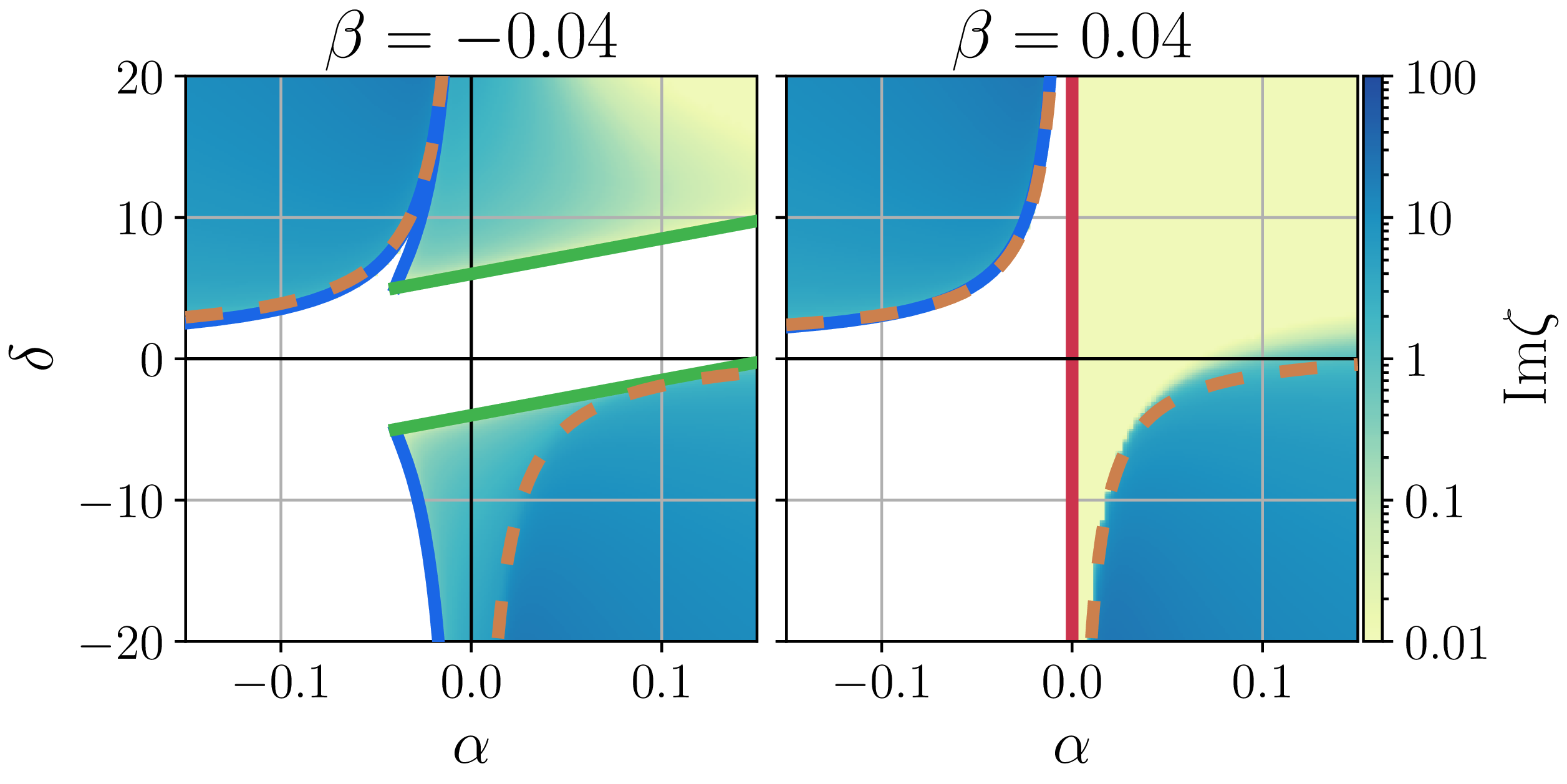


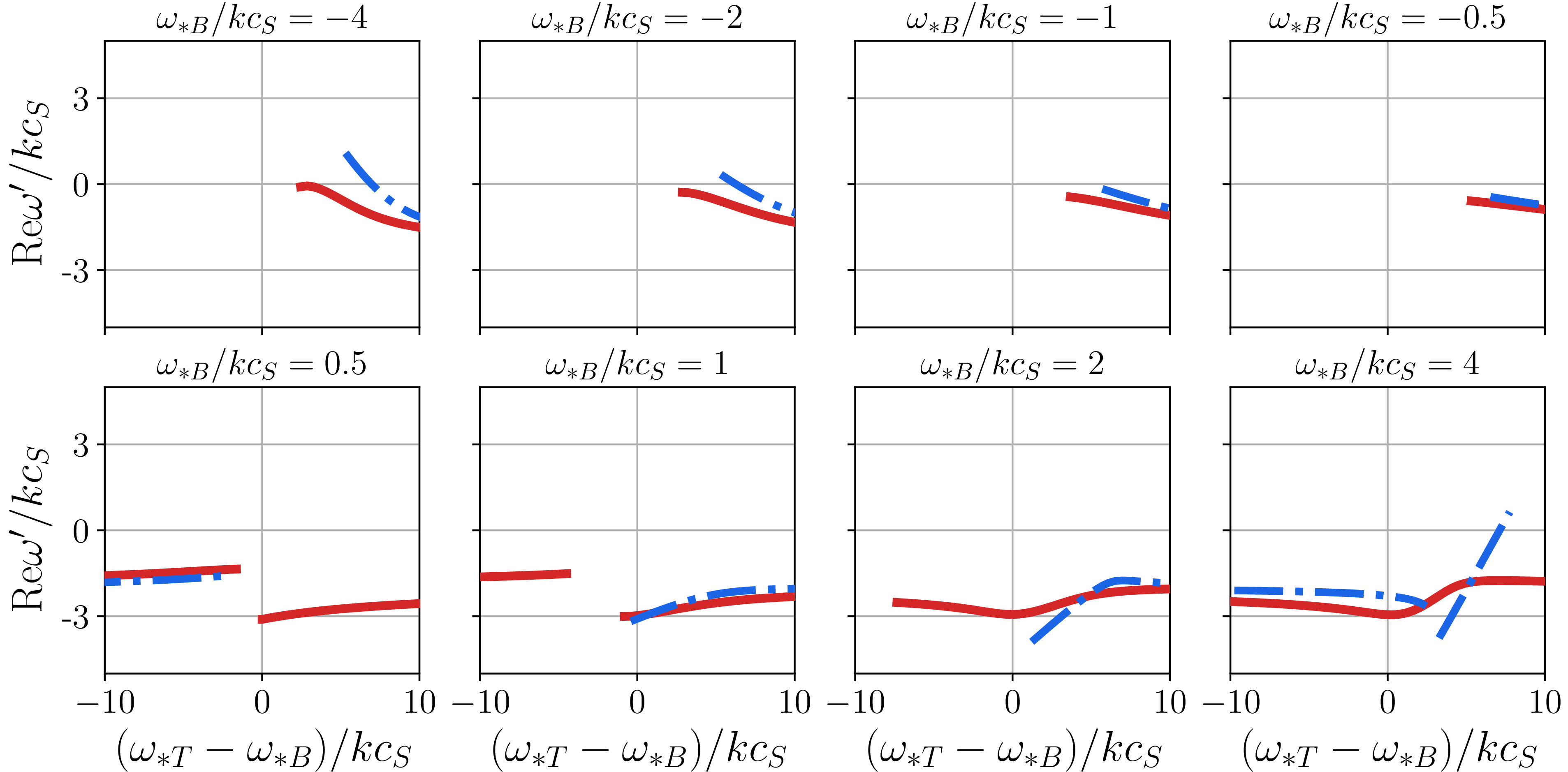


 Open access