





1. Introduction
Recent experimental and numerical investigations of turbulent wall-bounded flow have established that spanwise forcing through wall motion and wall jets, as both streamwise-travelling and standing waves, can be effective at reducing skin-friction drag at low Reynolds numbers ( $\textit{Re}_\tau \lesssim 1000$
), with skin-friction drag reductions of
$\textit{Re}_\tau \lesssim 1000$
), with skin-friction drag reductions of $\mathcal{DR}=20\,\%$
–
$\mathcal{DR}=20\,\%$
– $40\,\%$
frequently reported (Ricco, Skote & Leschziner Reference Ricco, Skote and Leschziner2021). However, this drag reduction has been shown to decay with Reynolds number (see e.g. Hurst, Yang & Chung Reference Hurst, Yang and Chung2014; Gatti Reference Gatti and Quadrio2016; Yao, Chen & Hussain Reference Yao, Chen and Hussain2019), which calls into question the effectiveness of spanwise forcing at the Reynolds numbers associated with flows of practical interest (e.g.
$40\,\%$
frequently reported (Ricco, Skote & Leschziner Reference Ricco, Skote and Leschziner2021). However, this drag reduction has been shown to decay with Reynolds number (see e.g. Hurst, Yang & Chung Reference Hurst, Yang and Chung2014; Gatti Reference Gatti and Quadrio2016; Yao, Chen & Hussain Reference Yao, Chen and Hussain2019), which calls into question the effectiveness of spanwise forcing at the Reynolds numbers associated with flows of practical interest (e.g. $\textit{Re}_\tau \sim 10^4$
–
$\textit{Re}_\tau \sim 10^4$
– $10^5$
for commercial aviation and shipping).
$10^5$
for commercial aviation and shipping).
This decrease in effectiveness has been attributed to the increasing importance of larger flow structures located farther from the wall than the spanwise forcing typically targets (see e.g. Touber & Leschziner Reference Touber and Leschziner2012; Agostini & Leschziner Reference Agostini and Leschziner2018; Yao et al. Reference Yao, Chen and Hussain2019). Approaches are thus sought which can directly interact with these larger-scale structures to induce skin-friction drag reduction. Since the importance of these structures grows with Reynolds number, it is hopeful that such a strategy will also lead to larger skin-friction reductions as the Reynolds number is increased.
The remainder of this section will discuss the various large-scale structures that are present in a turbulent boundary layer, how they impact skin-friction drag, and the various studies that have used jets in different configurations in an attempt to reduce skin-friction drag (including those directly targeting large-scale structures). This section will conclude with a discussion of the objectives and an introduction to the approach followed in the present study.
In the following, $x$
,
$x$
, $y$
and
$y$
and $z$
are the streamwise, wall-normal and spanwise coordinates, respectively, and the corresponding instantaneous velocities are
$z$
are the streamwise, wall-normal and spanwise coordinates, respectively, and the corresponding instantaneous velocities are $u$
,
$u$
, $v$
and
$v$
and $w$
, respectively. Reynolds decomposition of the velocity is used throughout to split instantaneous velocity into mean and fluctuating components; for example,
$w$
, respectively. Reynolds decomposition of the velocity is used throughout to split instantaneous velocity into mean and fluctuating components; for example, $u=\bar {u}+u'$
, where
$u=\bar {u}+u'$
, where $\bar {u}$
and
$\bar {u}$
and $u'$
are the mean and fluctuating streamwise velocity, respectively.
$u'$
are the mean and fluctuating streamwise velocity, respectively.
1.1. Large-scale structures in turbulent wall-bounded flow
In this work, ‘large-scale structures’ will refer to all coherent velocity structures with spatial scales larger than those associated with the near-wall cycle. This encompasses the induced coherent velocity structures from a hierarchy of wall-attached eddies that populate the logarithmic region of turbulent wall-bounded flow, as well as large-scale motions (LSMs) and very-large-scale motions (VLSMs)/superstructures.
Through particle image velocimetry (PIV) measurements in turbulent boundary layers at Reynolds numbers up to $\textit{Re}_\theta =6845$
, Meinhart & Adrian (Reference Meinhart and Adrian1995) showed that the turbulent boundary layer is composed instantaneously of many regions of nearly constant streamwise velocity, so called uniform momentum zones. Adrian, Meinhart & Tomkins (Reference Adrian, Meinhart and Tomkins2000) showed that the boundaries of these zones are populated with spanwise vortices and, using knowledge of the hairpin vortex signature from Zhou et al. (Reference Zhou, Adrian, Balachandar and Kendall1999), they inferred that the boundary layer consists of hairpin vortex packets, where hairpins (loosely defined as any vortical structure containing streamwise elongated leg(s) connected to relatively shorter spanwise vortical elements, whether symmetrical or not (i.e. canes, hairpins, horseshoes, etc.)) align in groups and collectively induce regions of low-speed fluid between their legs. The existence of hairpins, or packets thereof, is consistent with the attached-eddy hypothesis of Townsend (Reference Townsend1976), which describes wall-bounded turbulence as being dominated by self-similar wall-attached vortical structures whose size scales with distance from the wall. More recently, Baars, Hutchins & Marusic (Reference Baars, Hutchins and Marusic2017), for example, have also observed self-similarity of wall-attached turbulence through spectral coherence analysis of experimental data.
$\textit{Re}_\theta =6845$
, Meinhart & Adrian (Reference Meinhart and Adrian1995) showed that the turbulent boundary layer is composed instantaneously of many regions of nearly constant streamwise velocity, so called uniform momentum zones. Adrian, Meinhart & Tomkins (Reference Adrian, Meinhart and Tomkins2000) showed that the boundaries of these zones are populated with spanwise vortices and, using knowledge of the hairpin vortex signature from Zhou et al. (Reference Zhou, Adrian, Balachandar and Kendall1999), they inferred that the boundary layer consists of hairpin vortex packets, where hairpins (loosely defined as any vortical structure containing streamwise elongated leg(s) connected to relatively shorter spanwise vortical elements, whether symmetrical or not (i.e. canes, hairpins, horseshoes, etc.)) align in groups and collectively induce regions of low-speed fluid between their legs. The existence of hairpins, or packets thereof, is consistent with the attached-eddy hypothesis of Townsend (Reference Townsend1976), which describes wall-bounded turbulence as being dominated by self-similar wall-attached vortical structures whose size scales with distance from the wall. More recently, Baars, Hutchins & Marusic (Reference Baars, Hutchins and Marusic2017), for example, have also observed self-similarity of wall-attached turbulence through spectral coherence analysis of experimental data.
The LSMs are associated with the bulges of turbulent fluid that constitute the corrugated edge of the boundary layer. These bulges are of the order of $1\delta$
in streamwise length, are associated with the entrainment of non-turbulent fluid and have flow patterns consistent with a forward-rotating spanwise vortex (Kovasznay, Kibens & Blackwelder Reference Kovasznay, Kibens and Blackwelder1970; Blackwelder & Kovasznay Reference Blackwelder and Kovasznay1972).
$1\delta$
in streamwise length, are associated with the entrainment of non-turbulent fluid and have flow patterns consistent with a forward-rotating spanwise vortex (Kovasznay, Kibens & Blackwelder Reference Kovasznay, Kibens and Blackwelder1970; Blackwelder & Kovasznay Reference Blackwelder and Kovasznay1972).
VLSMs and superstructures are of the order of $10\delta$
in length (Kim & Adrian Reference Kim and Adrian1999; Guala, Hommema & Adrian Reference Guala, Hommema and Adrian2006; Hutchins & Marusic Reference Hutchins and Marusic2007a
), predominantly in the logarithmic region, although they extend across the entire layer. These structures are very energetic, contributing a large fraction of the total streamwise turbulent kinetic energy and Reynolds stress in wall-bounded flows (Guala et al. Reference Guala, Hommema and Adrian2006; Balakumar & Adrian Reference Balakumar and Adrian2007). Hairpin packets have also been speculated to form the LSMs, particularly at low Reynolds number (Adrian Reference Adrian2007), and a link between the superstructures and turbulent bulges has been suggested by Hutchins (Reference Hutchins2014). The VLSMs have been hypothesised to be due to a merging of hairpin packets or turbulent bulges (Kim & Adrian Reference Kim and Adrian1999), and there is a growing body of evidence to suggest that is the case (see e.g. Lee & Sung Reference Lee and Sung2011b
; Baltzer, Adrian & Wu Reference Baltzer, Adrian and Wu2013; Deshpande, de Silva & Marusic Reference Deshpande, de Silva and Marusic2023).
$10\delta$
in length (Kim & Adrian Reference Kim and Adrian1999; Guala, Hommema & Adrian Reference Guala, Hommema and Adrian2006; Hutchins & Marusic Reference Hutchins and Marusic2007a
), predominantly in the logarithmic region, although they extend across the entire layer. These structures are very energetic, contributing a large fraction of the total streamwise turbulent kinetic energy and Reynolds stress in wall-bounded flows (Guala et al. Reference Guala, Hommema and Adrian2006; Balakumar & Adrian Reference Balakumar and Adrian2007). Hairpin packets have also been speculated to form the LSMs, particularly at low Reynolds number (Adrian Reference Adrian2007), and a link between the superstructures and turbulent bulges has been suggested by Hutchins (Reference Hutchins2014). The VLSMs have been hypothesised to be due to a merging of hairpin packets or turbulent bulges (Kim & Adrian Reference Kim and Adrian1999), and there is a growing body of evidence to suggest that is the case (see e.g. Lee & Sung Reference Lee and Sung2011b
; Baltzer, Adrian & Wu Reference Baltzer, Adrian and Wu2013; Deshpande, de Silva & Marusic Reference Deshpande, de Silva and Marusic2023).
These large-scale structures are not independent of the smaller scales associated with the near-wall cycle, as they have an energetic ‘footprint’ in the near-wall region (Hutchins & Marusic Reference Hutchins and Marusic2007b ; Abe, Kawamura & Choi Reference Abe, Kawamura and Choi2004) and a modulating influence, in both amplitude and frequency, on the smaller scales (Brown & Thomas Reference Brown and Thomas1977; Bandyopadhyay & Hussain Reference Bandyopadhyay and Hussain1984; Hutchins & Marusic Reference Hutchins and Marusic2007b ; Mathis, Hutchins & Marusic Reference Mathis, Hutchins and Marusic2009; Ganapathisubramani et al. Reference Ganapathisubramani, Hutchins, Monty, Chung and Marusic2012). As the Reynolds number is increased, not only does the footprint of the large scales in the near-wall region increase, but the strength of the modulation increases in this region as well (Mathis et al. Reference Mathis, Hutchins and Marusic2009; Marusic, Mathis & Hutchins Reference Marusic, Mathis and Hutchins2010). The modulation in this region has been suggested to be related to the large-scale wall shear stress modification imposed by the large-scale velocity (Hutchins Reference Hutchins2014).
1.2. Skin-friction drag in turbulent wall-bounded flow
In low-Reynolds-number wall-bounded turbulent flow, the elevated skin friction relative to laminar flow is suggested to be due to the asymmetrical effect of streamwise vortices adjacent to the wall. These vortices pull down high-speed fluid and lift up low-speed fluid, which act to increase and decrease wall shear stress, respectively. However, the former process has been shown to have a larger impact on wall shear stress and, consequently, streamwise vortices induce a net increase in skin friction relative to a laminar boundary layer (Orlandi & Jiménez Reference Orlandi and Jiménez1994).
As the Reynolds number increases, Renard & Deck (Reference Renard and Deck2016) showed – using an energy-based decomposition of the skin-friction coefficient and primarily Reynolds-averaged Navier–Stokes simulations of turbulent boundary layers – that increasing turbulence production in the logarithmic region is responsible for an increasing proportion of the wall shear stress.
de Giovanetti, Hwang & Choi (Reference de Giovanetti, Hwang and Choi2016) also found that while the largest-scale motions (VLSMs and superstructures) contribute 20 $\%$
–30
$\%$
–30 $\%$
of the skin-friction drag at
$\%$
of the skin-friction drag at $\textit{Re}_\tau =2000$
, their removal only results in a skin-friction reduction of 5
$\textit{Re}_\tau =2000$
, their removal only results in a skin-friction reduction of 5 $\%$
–8
$\%$
–8 $\%$
. They suggested that this discrepancy could be due to a non-trivial scale interaction. Additionally, their results revealed that self-similar attached eddies, which populate the logarithmic region, generate the largest amount of skin friction at this Reynolds number.
$\%$
. They suggested that this discrepancy could be due to a non-trivial scale interaction. Additionally, their results revealed that self-similar attached eddies, which populate the logarithmic region, generate the largest amount of skin friction at this Reynolds number.
1.3. Skin-friction drag reduction using jets
Jets – steady, synthetic and pulsed – have been used frequently to interact with turbulent wall-bounded flow to attempt to induce skin-friction drag reduction. However, they have typically been limited to low Reynolds number and therefore focused on targeting the near-wall cycle.
Using direct numerical simulation (DNS) of turbulent channel flow at $\textit{Re}_\tau =180$
, Choi, Moin & Kim (Reference Choi, Moin and Kim1994) developed an opposition control scheme whereby velocity was prescribed at the wall to oppose the velocity induced by near-wall streamwise vortices. Using this numerical jet, they noted approximately a 20
$\textit{Re}_\tau =180$
, Choi, Moin & Kim (Reference Choi, Moin and Kim1994) developed an opposition control scheme whereby velocity was prescribed at the wall to oppose the velocity induced by near-wall streamwise vortices. Using this numerical jet, they noted approximately a 20 $\%$
–30
$\%$
–30 $\%$
reduction in skin friction. By using only surface sensing, a more practical approach, they noted only
$\%$
reduction in skin friction. By using only surface sensing, a more practical approach, they noted only $6\,\%$
drag reduction.
$6\,\%$
drag reduction.
In another DNS study, Park & Choi (Reference Park and Choi1999) used a two-dimensional (infinite span) slot with steady uniform blowing or suction on a low-Reynolds-number turbulent boundary layer ( $\textit{Re}_\tau \approx 150$
–
$\textit{Re}_\tau \approx 150$
– $250$
) with blowing ratios – the ratio of jet velocity to free stream velocity
$250$
) with blowing ratios – the ratio of jet velocity to free stream velocity $r=U_{\!j}/U_\infty$
– less than
$r=U_{\!j}/U_\infty$
– less than $r=0.1$
. They noticed that, even with this weak blowing, the near-wall streamwise vortices were lifted up and interacted more weakly with the wall, which resulted in a large reduction of skin friction close to the slot. Further downstream though, the vortices were able to grow stronger due to weaker diffusion. Along with stronger stretching and tilting, the skin friction became higher downstream. Essentially the opposite effect was seen for suction. The extent of the skin-friction changes and the relaxation length were also seen to grow with blowing/suction amplitude.
$r=0.1$
. They noticed that, even with this weak blowing, the near-wall streamwise vortices were lifted up and interacted more weakly with the wall, which resulted in a large reduction of skin friction close to the slot. Further downstream though, the vortices were able to grow stronger due to weaker diffusion. Along with stronger stretching and tilting, the skin friction became higher downstream. Essentially the opposite effect was seen for suction. The extent of the skin-friction changes and the relaxation length were also seen to grow with blowing/suction amplitude.
Other studies, such as Tardu (Reference Tardu2001) (experimental with spanwise-elongated orifice of aspect ratio $\textit{AR}=167$
) and Kim & Sung (Reference Kim and Sung2006) (DNS with infinite spanwise-elongated orifice), have investigated periodic blowing and noticed similar effects to steady blowing, albeit with slight differences. For example, Kim & Sung (Reference Kim and Sung2006) noticed that while steady blowing results locally in a maximum skin-friction decrease of
$\textit{AR}=167$
) and Kim & Sung (Reference Kim and Sung2006) (DNS with infinite spanwise-elongated orifice), have investigated periodic blowing and noticed similar effects to steady blowing, albeit with slight differences. For example, Kim & Sung (Reference Kim and Sung2006) noticed that while steady blowing results locally in a maximum skin-friction decrease of $77\,\%$
very near the jet orifice, periodic blowing can result in weaker maximum skin-friction reductions and larger increases in skin friction further downstream.
$77\,\%$
very near the jet orifice, periodic blowing can result in weaker maximum skin-friction reductions and larger increases in skin friction further downstream.
Park, Lee & Sung (Reference Park, Lee and Sung2001) used a synthetic jet in a turbulent boundary layer (experimental with spanwise-elongated orifice of $\textit{AR}=60$
) and noted skin-friction drag reductions of up to 45
$\textit{AR}=60$
) and noted skin-friction drag reductions of up to 45 $\%$
at their initial location, approximately
$\%$
at their initial location, approximately $0.25\delta$
downstream of the orifice. At their final location, approximately
$0.25\delta$
downstream of the orifice. At their final location, approximately $2.1\delta$
downstream of the orifice, the two lower frequency jets,
$2.1\delta$
downstream of the orifice, the two lower frequency jets, $St_h\approx 0.05$
and
$St_h\approx 0.05$
and $St_h\approx 0.1$
, where
$St_h\approx 0.1$
, where $St_h=fh/U_\infty$
is the Strouhal number based on streamwise slot dimension
$St_h=fh/U_\infty$
is the Strouhal number based on streamwise slot dimension $h$
and frequency
$h$
and frequency $f$
, recovered to the baseline skin-friction value, while they noted a skin-friction reduction of approximately
$f$
, recovered to the baseline skin-friction value, while they noted a skin-friction reduction of approximately $2\,\%$
for the highest frequency case,
$2\,\%$
for the highest frequency case, $St_h\approx 0.2$
. They believed that the skin-friction reduction is due to an upward shift of the mean velocity profile. At the same time, they noted an increase in the displacement thickness that stays elevated at approximately
$St_h\approx 0.2$
. They believed that the skin-friction reduction is due to an upward shift of the mean velocity profile. At the same time, they noted an increase in the displacement thickness that stays elevated at approximately $3$
%–
$3$
%– $7$
% at
$7$
% at $x/\delta =2.1$
for the cases tested, which has consequences for pressure drag on curved surfaces.
$x/\delta =2.1$
for the cases tested, which has consequences for pressure drag on curved surfaces.
In addition to spanwise-elongated jets, studies have also investigated the effect of jets from streamwise-aligned rectangular orifices. For example, in an experimental study, Rathnasingham & Breuer (Reference Rathnasingham and Breuer2003) used a spanwise array of streamwise-aligned synthetic jets ( $\textit{AR}=15$
) in a turbulent boundary layer (
$\textit{AR}=15$
) in a turbulent boundary layer ( $\textit{Re}_\tau \approx 650$
) to introduce low-speed streaks that counteract near-wall structures and disrupt the near-wall cycle within an active control framework. While the control scheme was not designed to reduce skin friction, they noticed a 7
$\textit{Re}_\tau \approx 650$
) to introduce low-speed streaks that counteract near-wall structures and disrupt the near-wall cycle within an active control framework. While the control scheme was not designed to reduce skin friction, they noticed a 7 $\%$
reduction in skin friction downstream of the actuator array.
$\%$
reduction in skin friction downstream of the actuator array.
In a recent experimental study, Cheng et al. (Reference Cheng, Qiao, Zhang, Quadrio and Zhou2021) used low-amplitude periodic blowing, similar to Tardu (Reference Tardu2001) and Kim & Sung (Reference Kim and Sung2006), but from a spanwise array of streamwise-aligned orifices ( $\textit{AR}=40$
) in an
$\textit{AR}=40$
) in an $\textit{Re}_\tau \approx 570$
turbulent boundary layer. A parametric study of the amplitude and frequency of the blowing was performed, and a maximum local skin friction reduction of
$\textit{Re}_\tau \approx 570$
turbulent boundary layer. A parametric study of the amplitude and frequency of the blowing was performed, and a maximum local skin friction reduction of ${\gt} 70\,\%$
was noted along with achievable net power saving. Visualisation indicated stabilised streaks and a locally relaminarised flow, and additional analysis suggested that
${\gt} 70\,\%$
was noted along with achievable net power saving. Visualisation indicated stabilised streaks and a locally relaminarised flow, and additional analysis suggested that $77\,\%$
of the drag reduction was due to a reduction in the mean streamwise velocity gradient due to the injection of zero-streamwise-momentum fluid, while the remaining
$77\,\%$
of the drag reduction was due to a reduction in the mean streamwise velocity gradient due to the injection of zero-streamwise-momentum fluid, while the remaining $23\,\%$
was due to the formation of streamwise vortices interrupting the near-wall cycle.
$23\,\%$
was due to the formation of streamwise vortices interrupting the near-wall cycle.
Another recent experiment by Abbassi et al. (Reference Abbassi, Baars, Hutchins and Marusic2017) used a spanwise array of nine streamwise-aligned jets ( $\textit{AR}=25$
) which spanned approximately
$\textit{AR}=25$
) which spanned approximately $0.6\delta$
to interact with large-scale structures (
$0.6\delta$
to interact with large-scale structures ( $\lambda _x/\delta \gt 2$
, primarily LSMs and VLSMs) in a high-Reynolds-number turbulent boundary layer (
$\lambda _x/\delta \gt 2$
, primarily LSMs and VLSMs) in a high-Reynolds-number turbulent boundary layer ( $\textit{Re}_\tau =14\,400$
). This was done in conjunction with upstream wall-shear-stress sensors to determine the passage of large-scale wall-shear-stress events associated with wall-coherent large-scale structures. The wall-normal jets were triggered on positive large-scale fluctuations upstream to counteract the downward movement of fluid associated with the roll modes of the structures, similar to the opposition control of Choi et al. (Reference Choi, Moin and Kim1994). Through measurements of the wall shear stress downstream, they noticed that the skin friction could be decreased by approximately 3.2
$\textit{Re}_\tau =14\,400$
). This was done in conjunction with upstream wall-shear-stress sensors to determine the passage of large-scale wall-shear-stress events associated with wall-coherent large-scale structures. The wall-normal jets were triggered on positive large-scale fluctuations upstream to counteract the downward movement of fluid associated with the roll modes of the structures, similar to the opposition control of Choi et al. (Reference Choi, Moin and Kim1994). Through measurements of the wall shear stress downstream, they noticed that the skin friction could be decreased by approximately 3.2 $\%$
with this scheme, although both reductions of 2.4
$\%$
with this scheme, although both reductions of 2.4 $\%$
and 1.2
$\%$
and 1.2 $\%$
were seen for ‘desynchronised’ (i.e. blowing according to high-speed regions from a previous run) and reinforcing blowing (i.e. blowing into low-speed regions), respectively. They also noted a significant decrease in the large-scale fluctuations (up to 33
$\%$
were seen for ‘desynchronised’ (i.e. blowing according to high-speed regions from a previous run) and reinforcing blowing (i.e. blowing into low-speed regions), respectively. They also noted a significant decrease in the large-scale fluctuations (up to 33 $\%$
for wavelengths longer than
$\%$
for wavelengths longer than $5\delta$
) throughout the boundary layer due to the forcing.
$5\delta$
) throughout the boundary layer due to the forcing.
Dacome et al. (Reference Dacome, Mörsch, Kotsonis and Baars2024), building on the work of Abbassi et al. (Reference Abbassi, Baars, Hutchins and Marusic2017), used a single $\textit{AR}=10$
streamwise-aligned jet at a blowing ratio of
$\textit{AR}=10$
streamwise-aligned jet at a blowing ratio of $r=0.4$
downstream of a hot-film wall-shear-stress sensor in an
$r=0.4$
downstream of a hot-film wall-shear-stress sensor in an $\textit{Re}_\tau =2240$
turbulent boundary layer. They presented similar results to Abbassi et al. (Reference Abbassi, Baars, Hutchins and Marusic2017): opposing control reduced skin friction 2 %–3 % with respect to desynchronised control and had similar effects on large-scale fluctuations, although they showed a larger 7 %–11 % reduction relative to the uncontrolled case.
$\textit{Re}_\tau =2240$
turbulent boundary layer. They presented similar results to Abbassi et al. (Reference Abbassi, Baars, Hutchins and Marusic2017): opposing control reduced skin friction 2 %–3 % with respect to desynchronised control and had similar effects on large-scale fluctuations, although they showed a larger 7 %–11 % reduction relative to the uncontrolled case.
1.4. Objective and structure of this paper
In the present study, synthetic jets ejected in the wall-normal direction through a rectangular orifice are used to interact with large-scale structures in the logarithmic region of a turbulent boundary layer. While the overarching goal is to identify a skin-friction reduction mechanism that scales favourably with Reynolds number, achieving net drag reduction and power savings requires investigation of the entire jet-influenced region. Thus, the objective of this work is to investigate the impact on the multi-scale structure of streamwise velocity and its consequent impact on wall shear stress/skin friction throughout the spatial extent of the region of influence of the synthetic jet. This is in contrast to Abbassi et al. (Reference Abbassi, Baars, Hutchins and Marusic2017) and Dacome et al. (Reference Dacome, Mörsch, Kotsonis and Baars2024), where measurements were taken at a single location downstream of the jet exit.
The spanwise dimension of the synthetic-jet orifice was chosen to match the dominant lengthscales in the logarithmic region of the boundary layer and the jets were operated in an open loop configuration. Thus, the forcing does not preferentially target motions of a certain scale (opposition control), as in Abbassi et al. (Reference Abbassi, Baars, Hutchins and Marusic2017) and Dacome et al. (Reference Dacome, Mörsch, Kotsonis and Baars2024) for example, but rather targets all scales of size less than or equal to the orifice width simultaneously. This is preferred due to the wide range of scales present in the logarithmic region that contribute to skin friction. As the focus of this study is on the physics of the interaction and neither the synthetic jet actuator nor the actuation scheme are optimised, the full energy budget is not considered in this study.
Wind-tunnel experiments and large eddy simulation (LES) are used to investigate the nature of the interaction, with LES focusing on the region $x/\delta \lt 2$
, where the effects are stronger and the temporal requirement for statistical convergence is less stringent, and hot-film and hot-wire measurements are performed in a wind tunnel for
$x/\delta \lt 2$
, where the effects are stronger and the temporal requirement for statistical convergence is less stringent, and hot-film and hot-wire measurements are performed in a wind tunnel for $x/\delta \gt 2$
, where vertical velocity and recirculation from the synthetic jets have less effect on the heat transfer. Results from both experiment and simulation at the same location will be presented in the following where practical. A more complete comparison of the simulations and experiments at
$x/\delta \gt 2$
, where vertical velocity and recirculation from the synthetic jets have less effect on the heat transfer. Results from both experiment and simulation at the same location will be presented in the following where practical. A more complete comparison of the simulations and experiments at $x/\delta =2$
is contained in Appendix A.2.
$x/\delta =2$
is contained in Appendix A.2.
The structure of the remainder of this paper is as follows. In § 2, details of the experimental and numerical set-up are presented. The effect of the synthetic jet forcing on the large-scale structures and the consequent impact on wall shear stress are presented in § 3.1 at both $x/\delta =2$
and
$x/\delta =2$
and $x/\delta =5$
. Additional insights into the causes of the changes to the wall shear stress are provided in this section by investigating changes to the boundary-layer velocity and correlating changes to the mean wall shear stress with changes to the magnitude of small- and large-scale wall shear stress fluctuations. In § 5, the synthetic-jet coherent structures are investigated for select forcing conditions using large eddy simulation to understand their direct impact on wall shear stress closer to the synthetic-jet orifice and at the spanwise edges of the jet. Concluding remarks are provided in § 6.
$x/\delta =5$
. Additional insights into the causes of the changes to the wall shear stress are provided in this section by investigating changes to the boundary-layer velocity and correlating changes to the mean wall shear stress with changes to the magnitude of small- and large-scale wall shear stress fluctuations. In § 5, the synthetic-jet coherent structures are investigated for select forcing conditions using large eddy simulation to understand their direct impact on wall shear stress closer to the synthetic-jet orifice and at the spanwise edges of the jet. Concluding remarks are provided in § 6.
2. Experimental and numerical details
As mentioned previously, both wind-tunnel experiments and LES were conducted to gather complementary information about the effect of the synthetic jets on the turbulent boundary layer. Hot-wire and hot-film measurements in the boundary layer are suitable for obtaining well-converged statistics and temporally resolved results of a single velocity or stress component across a range of scales at select locations, while simulations are more suitable for obtaining three-dimensional spatial information (albeit less temporally converged). In addition, due to the much stronger cross-stream velocity components, and as will be shown later, recirculation, close to the orifice ( $x/\delta \lt 2$
), hot wires and hot films are unsuitable in this region for accurately measuring boundary-layer velocity and wall shear stress, respectively. Further downstream (
$x/\delta \lt 2$
), hot wires and hot films are unsuitable in this region for accurately measuring boundary-layer velocity and wall shear stress, respectively. Further downstream ( $x/\delta \gt 5$
), it is not practical to achieve the statistics required for sufficiently converged results using the simulations due to the relatively weaker effects on the turbulent boundary layer. Thus, in this work, we primarily use the simulations to understand the effect of the synthetic jets on the boundary layer for
$x/\delta \gt 5$
), it is not practical to achieve the statistics required for sufficiently converged results using the simulations due to the relatively weaker effects on the turbulent boundary layer. Thus, in this work, we primarily use the simulations to understand the effect of the synthetic jets on the boundary layer for $x/\delta \lt 2$
and the hot-wire/hot-film measurements for
$x/\delta \lt 2$
and the hot-wire/hot-film measurements for $x/\delta \gt 2$
.
$x/\delta \gt 2$
.
To validate the simulations, PIV was performed along the jet centreline for various synthetic-jet forcing conditions and the effect on boundary-layer velocity was compared with matching results from the simulations. The methods and results for this, as well as comparisons between simulation and experiment at the overlap, $x/\delta =2$
, are contained in Appendix A.
$x/\delta =2$
, are contained in Appendix A.
2.1. Experimental details
All experimental measurements were taken in the low-speed recirculating wind tunnel at the University of Toronto Institute for Aerospace Studies (for more information, see Hearst Reference Hearst2015). The working region of the wind tunnel consists of two test sections each measuring $2.5\ {\textrm{m}}$
in length (5 m in total) in the streamwise direction. The cross-section of the test sections is octagonal with a fixed width and height of
$2.5\ {\textrm{m}}$
in length (5 m in total) in the streamwise direction. The cross-section of the test sections is octagonal with a fixed width and height of $1.2\ {\textrm{m}}$
and
$1.2\ {\textrm{m}}$
and $0.8\ {\textrm{m}}$
, respectively.
$0.8\ {\textrm{m}}$
, respectively.
A series of three 12.7 mm-thick aluminium plates were installed in the test sections, which extend the width of the test sections (see figure 1
a). The combined length of these three plates is $5\ {\textrm{m}}$
, such that they also extend the combined length of the two test sections. Four independently adjustable legs on the bottom of each plate lifted the boundary-layer plate approximately a third of the test-section height above the floor to prevent interaction between the test-section boundary layers and those on the plates. A zero pressure gradient was established by adjusting fillets at the corners of the test section and slightly adjusting the angle of attack of the plate. An asymmetrical leading edge, which is optimised to minimise unwanted adverse pressure gradients at the leading edge (Hanson, Buckley & Lavoie Reference Hanson, Buckley and Lavoie2012), was installed at the upstream end of the first plate, and a hinged plate was connected at the downstream end of the last plate to control circulation around the plate and the stagnation line. A double-layer of zig–zag tape was installed a small distance (
$5\ {\textrm{m}}$
, such that they also extend the combined length of the two test sections. Four independently adjustable legs on the bottom of each plate lifted the boundary-layer plate approximately a third of the test-section height above the floor to prevent interaction between the test-section boundary layers and those on the plates. A zero pressure gradient was established by adjusting fillets at the corners of the test section and slightly adjusting the angle of attack of the plate. An asymmetrical leading edge, which is optimised to minimise unwanted adverse pressure gradients at the leading edge (Hanson, Buckley & Lavoie Reference Hanson, Buckley and Lavoie2012), was installed at the upstream end of the first plate, and a hinged plate was connected at the downstream end of the last plate to control circulation around the plate and the stagnation line. A double-layer of zig–zag tape was installed a small distance ( ${\sim}10$
cm) downstream of the leading edge to ensure a predictable spanwise-homogeneous transition to turbulence.
${\sim}10$
cm) downstream of the leading edge to ensure a predictable spanwise-homogeneous transition to turbulence.
Schematics of the (a) boundary layer plate and (b) synthetic-jet actuator (in deconstructed view).

For synthetic-jet actuation, a $20\ \textrm {cm}$ $\times$ $20\ \textrm {cm}$
removable flush-mounted synthetic-jet actuator plate was installed 2.7 m downstream of the leading edge and centred in the span. The synthetic-jet actuator used in this work consisted of a Visaton SC 8N loudspeaker oscillating against an aluminium disk-shaped cavity. This cavity had an opening that exited to a three-dimensional (3-D)-printed plastic insert which served to interface with the boundary-layer fluid through an orifice of rectangular cross-section (see figure 1
b). This orifice was oriented such that the long axis, measuring
$20\ \textrm {cm}$
removable flush-mounted synthetic-jet actuator plate was installed 2.7 m downstream of the leading edge and centred in the span. The synthetic-jet actuator used in this work consisted of a Visaton SC 8N loudspeaker oscillating against an aluminium disk-shaped cavity. This cavity had an opening that exited to a three-dimensional (3-D)-printed plastic insert which served to interface with the boundary-layer fluid through an orifice of rectangular cross-section (see figure 1
b). This orifice was oriented such that the long axis, measuring $l=13$
mm, was along the spanwise direction and the short axis, measuring
$l=13$
mm, was along the spanwise direction and the short axis, measuring $h=1$
mm, was along the streamwise direction (for an aspect ratio of
$h=1$
mm, was along the streamwise direction (for an aspect ratio of $\textit{AR}=13$
). Since the target of the actuation is large-scale structures in the logarithmic region of the turbulent boundary layer, the spanwise length of the orifice was scaled to match the spanwise extent of those structures. In the logarithmic region, the dominant large-scale structures have spanwise length scales of 0.1
$\textit{AR}=13$
). Since the target of the actuation is large-scale structures in the logarithmic region of the turbulent boundary layer, the spanwise length of the orifice was scaled to match the spanwise extent of those structures. In the logarithmic region, the dominant large-scale structures have spanwise length scales of 0.1 $\delta$
to 0.5
$\delta$
to 0.5 $\delta$
(Tomkins & Adrian Reference Tomkins and Adrian2003; Lee & Sung Reference Lee and Sung2011b
). A representative value in this range is
$\delta$
(Tomkins & Adrian Reference Tomkins and Adrian2003; Lee & Sung Reference Lee and Sung2011b
). A representative value in this range is $0.3\delta$
, which corresponds to approximately 13 mm for the boundary layer that is considered in this work. To drive the loudspeaker, a dual-channel Rigol DG 1022 function generator was used to provide a sinusoidal signal which was amplified by a Crown XTi 1002 stereo amplifier before being fed to the loudspeaker.
$0.3\delta$
, which corresponds to approximately 13 mm for the boundary layer that is considered in this work. To drive the loudspeaker, a dual-channel Rigol DG 1022 function generator was used to provide a sinusoidal signal which was amplified by a Crown XTi 1002 stereo amplifier before being fed to the loudspeaker.
Measurements of streamwise velocity and wall shear stress were acquired by hot-wire and hot-film anemometry, respectively. The hot wires were fabricated in-house and consisted of copper-coated $5\ \mu {\textrm{m}}$
tungsten wire with an exposed region measuring nominally
$5\ \mu {\textrm{m}}$
tungsten wire with an exposed region measuring nominally $1\ \textrm {mm}$
in length. This amounts to
$1\ \textrm {mm}$
in length. This amounts to $l^+\approx 25$
and
$l^+\approx 25$
and $l/d\approx 200$
, which adheres to the recommendations of Ligrani & Bradshaw (Reference Ligrani and Bradshaw1987). The hot films were wall-mounted Tao Systems Senflex SF9902 and SF9902M hot-film sensors with a spanwise length corresponding to
$l/d\approx 200$
, which adheres to the recommendations of Ligrani & Bradshaw (Reference Ligrani and Bradshaw1987). The hot films were wall-mounted Tao Systems Senflex SF9902 and SF9902M hot-film sensors with a spanwise length corresponding to $l^+\approx 35$
. A Dantec StreamLine 90N10 constant-temperature anemometer was used to set the hot wires and hot films at constant overheat ratios of 1.6 and 1.4, respectively. The signals obtained from the hot wires and hot films were low-pass filtered at 9–10 kHz to remove high-frequency non-turbulent noise before being sampled at a rate of 25 kHz using a National Instruments PCIe-6259 DAQ.
$l^+\approx 35$
. A Dantec StreamLine 90N10 constant-temperature anemometer was used to set the hot wires and hot films at constant overheat ratios of 1.6 and 1.4, respectively. The signals obtained from the hot wires and hot films were low-pass filtered at 9–10 kHz to remove high-frequency non-turbulent noise before being sampled at a rate of 25 kHz using a National Instruments PCIe-6259 DAQ.
All measurements were collected at a fixed free stream velocity of $U_\infty =10$
ms−1. At the location of the synthetic-jet orifice, this corresponds to a boundary-layer thickness of
$U_\infty =10$
ms−1. At the location of the synthetic-jet orifice, this corresponds to a boundary-layer thickness of $\delta \approx 42$
mm and a Reynolds number of
$\delta \approx 42$
mm and a Reynolds number of $\textit{Re}_\tau =1100$
. Wall shear stress data were collected at four locations (see figure 2):
$\textit{Re}_\tau =1100$
. Wall shear stress data were collected at four locations (see figure 2): $x/\delta =2$
and
$x/\delta =2$
and $x/\delta =5$
downstream of the orifice centreline (
$x/\delta =5$
downstream of the orifice centreline ( $z/l=0$
), and
$z/l=0$
), and $x/\delta =2$
and
$x/\delta =2$
and $x/\delta =5$
downstream of the orifice edge (
$x/\delta =5$
downstream of the orifice edge ( $z/l=0.5$
). Streamwise velocity data were collected at both
$z/l=0.5$
). Streamwise velocity data were collected at both $x/\delta =2$
and
$x/\delta =2$
and $x/\delta =5$
at 44 wall-normal locations from approximately
$x/\delta =5$
at 44 wall-normal locations from approximately $y^+=5$
to
$y^+=5$
to $y/\delta =2$
and at seven spanwise locations from
$y/\delta =2$
and at seven spanwise locations from $z/l=0$
to
$z/l=0$
to $z/l=1$
in equally spaced steps of
$z/l=1$
in equally spaced steps of $\Delta z/l=0.167$
. The
$\Delta z/l=0.167$
. The $x/\delta =2$
location was chosen as the most upstream location where hot-wire measurements were not appreciably affected by cross-stream velocity components induced by the strongest synthetic jet tested. The
$x/\delta =2$
location was chosen as the most upstream location where hot-wire measurements were not appreciably affected by cross-stream velocity components induced by the strongest synthetic jet tested. The $x/\delta =5$
location was chosen to evaluate the downstream development of the interaction, while ensuring the effect remained sufficiently strong to be measurable for the weakest synthetic jet tested.
$x/\delta =5$
location was chosen to evaluate the downstream development of the interaction, while ensuring the effect remained sufficiently strong to be measurable for the weakest synthetic jet tested.
Top-down schematic of the boundary layer plate showing the synthetic-jet orifice and the wall-shear-stress measurement locations, which are marked with an $\boldsymbol{\times}$
.
$\boldsymbol{\times}$
.

2.2. Numerical details
LES was performed using Diablo, an in-house compressible Newton–Krylov–Schur flow solver (for details, see Hicken & Zingg Reference Hicken and Zingg2008; Osusky & Zingg Reference Osusky and Zingg2013; Boom, Rolston & Zingg Reference Boom, Rolston and Zingg2018). Diablo is a parallel implicit flow solver capable of solving both steady and unsteady problems. Additionally, it is applicable to block-structured meshes and is high-order in both space and time.
Zero-pressure-gradient flat-plate turbulent-boundary-layer simulations were conducted at a fixed Mach number of $M_\infty =U_\infty /a_\infty =0.2$
, where
$M_\infty =U_\infty /a_\infty =0.2$
, where $a_\infty$
is the free stream speed of sound, and a target friction Reynolds number of
$a_\infty$
is the free stream speed of sound, and a target friction Reynolds number of $\textit{Re}_\tau =1100$
. The Mach number was chosen for optimal performance of the flow solver without adding significant compressibility effects and the Reynolds number was chosen to match the experiments.
$\textit{Re}_\tau =1100$
. The Mach number was chosen for optimal performance of the flow solver without adding significant compressibility effects and the Reynolds number was chosen to match the experiments.
The simulations were conducted on a rectilinear multi-block structured grid, as shown in figure 3. The domain extends $25\,\delta _0$
in the streamwise direction, where
$25\,\delta _0$
in the streamwise direction, where $\delta _0$
is the target boundary-layer thickness at
$\delta _0$
is the target boundary-layer thickness at $x/\delta _0=15$
. In the wall-normal direction, the domain extends
$x/\delta _0=15$
. In the wall-normal direction, the domain extends $4 \,\delta _0$
to limit the influence of the upper wall on the boundary layer. Finally, in the spanwise direction, the domain extends
$4 \,\delta _0$
to limit the influence of the upper wall on the boundary layer. Finally, in the spanwise direction, the domain extends $3\,\delta _0$
, which is a few times larger than the largest spanwise scales (see e.g. Cantwell Reference Cantwell1981). For simulations of synthetic-jet-actuated turbulent boundary layers, a slot was also extruded
$3\,\delta _0$
, which is a few times larger than the largest spanwise scales (see e.g. Cantwell Reference Cantwell1981). For simulations of synthetic-jet-actuated turbulent boundary layers, a slot was also extruded $0.075\,\delta _0$
below the
$0.075\,\delta _0$
below the $y/\delta _0=0$
plane at
$y/\delta _0=0$
plane at $x/\delta _0=15$
for the synthetic jet.
$x/\delta _0=15$
for the synthetic jet.
Flow domain and grid structure for flat-plate turbulent-boundary-layer simulations. (a) Domain block structure. Inset shows the block grid. (b) Refined grid in vicinity of synthetic-jet slot (green).

For the uncontrolled grids, the spacing in the streamwise and spanwise directions was uniform (with some refinement near block interfaces), while in the wall-normal direction, the grid was stretched according to a hyperbolic tangent relation up to $y/\delta _0=2$
, above which it was uniform. For simulations with synthetic-jet actuation, the grid was refined in
$y/\delta _0=2$
, above which it was uniform. For simulations with synthetic-jet actuation, the grid was refined in $x$
and
$x$
and $z$
in the vicinity of the synthetic-jet slot.
$z$
in the vicinity of the synthetic-jet slot.
Table 1 contains more information about the grids used in this study, including the number of nodes in each of the coordinate directions ( $N_x$
,
$N_x$
, $N_y$
,
$N_y$
, $N_z$
), the spacing in each of the coordinate directions (
$N_z$
), the spacing in each of the coordinate directions ( $\Delta x$
,
$\Delta x$
, $\Delta y$
,
$\Delta y$
, $\Delta z$
) and the total number of nodes (
$\Delta z$
) and the total number of nodes ( $N_{\textit{total}}$
). Typical grid spacing for DNS of flat-plate turbulent boundary layers is
$N_{\textit{total}}$
). Typical grid spacing for DNS of flat-plate turbulent boundary layers is $\Delta x^+\approx$
6–16,
$\Delta x^+\approx$
6–16, $\Delta y^+_{\textit{min}}\approx$
0.06–1.3 (
$\Delta y^+_{\textit{min}}\approx$
0.06–1.3 ( $\Delta y^+_{\textit{a}v\textit{g}}\approx$
6–20) and
$\Delta y^+_{\textit{a}v\textit{g}}\approx$
6–20) and $\Delta z^+\approx$
4–7 (see e.g. Ferrante & Elghobashi Reference Ferrante and Elghobashi2005; Simens et al. Reference Simens, Jiménez, Hoyas and Mizuno2009; Lee & Sung Reference Lee and Sung2011a
). Comparing this to the grid spacing in table 1, the spanwise and wall-normal dimensions are well resolved in the present simulations, but the streamwise dimension is under resolved by approximately a factor of two. Estimating from the DNS channel flow spectra of del Álamo et al. (Reference del Álamo, Jiménez, Zandonade and Moser2004) (data accessed from https://torroja.dmt.upm.es/channels/data/spectra/) at
$\Delta z^+\approx$
4–7 (see e.g. Ferrante & Elghobashi Reference Ferrante and Elghobashi2005; Simens et al. Reference Simens, Jiménez, Hoyas and Mizuno2009; Lee & Sung Reference Lee and Sung2011a
). Comparing this to the grid spacing in table 1, the spanwise and wall-normal dimensions are well resolved in the present simulations, but the streamwise dimension is under resolved by approximately a factor of two. Estimating from the DNS channel flow spectra of del Álamo et al. (Reference del Álamo, Jiménez, Zandonade and Moser2004) (data accessed from https://torroja.dmt.upm.es/channels/data/spectra/) at $\textit{Re}_\tau =950$
, with our level of refinement in
$\textit{Re}_\tau =950$
, with our level of refinement in $x$
, the small-scale fluctuations which we do not resolve are expected to account for approximately 0.5 %, 2.5 % and 1.5 % of
$x$
, the small-scale fluctuations which we do not resolve are expected to account for approximately 0.5 %, 2.5 % and 1.5 % of $\overline {u'}^2$
,
$\overline {u'}^2$
, $\overline {v'}^2$
and
$\overline {v'}^2$
and $\overline {w'}^2$
, respectively. With our level of refinement in
$\overline {w'}^2$
, respectively. With our level of refinement in $z$
, the small-scale fluctuations are expected to account for
$z$
, the small-scale fluctuations are expected to account for $\lt 0.5\,\%$
for each of
$\lt 0.5\,\%$
for each of $\overline {u'}^2$
,
$\overline {u'}^2$
, $\overline {v'}^2$
and
$\overline {v'}^2$
and $\overline {w'}^2$
.
$\overline {w'}^2$
.
Grid information for the uncontrolled and controlled simulations.

Each grid was split into blocks each consisting of $33^3$
nodes (see figure 3
a). For the grids listed in table 1, this corresponds to 3696 and 3698 blocks for uncontrolled and controlled, respectively. The solution on each block was computed in parallel with parallel simulation handled using the Message Passing Interface (MPI) on a separate core of the 40-core nodes of the Niagara cluster, maintained by the Digital Research Alliance of Canada.
$33^3$
nodes (see figure 3
a). For the grids listed in table 1, this corresponds to 3696 and 3698 blocks for uncontrolled and controlled, respectively. The solution on each block was computed in parallel with parallel simulation handled using the Message Passing Interface (MPI) on a separate core of the 40-core nodes of the Niagara cluster, maintained by the Digital Research Alliance of Canada.
The Navier–Stokes equations were discretely approximated in space using third-order (sixth-order on the interior) summation-by-parts operators with time integration using a second-order explicit-first-stage diagonally implicit Runge–Kutta method. No explicit subgrid-scale model was employed in this work; instead, dissipation of unresolved small scales was controlled using a minimal amount of matrix artificial dissipation consistent with the summation-by-parts operators. Thus, these simulations can be described as either slightly under-resolved direct numerical simulation or well-resolved implicit large eddy simulation.
In the wall-normal direction, an adiabatic no-slip boundary condition was used at the wall, and a zeroth-order extrapolation of the solution from the interior was used at the top of the domain, which is equivalent to a first-order approximation to $\partial {\boldsymbol{u}}/\partial y=0$
.
$\partial {\boldsymbol{u}}/\partial y=0$
.
In the streamwise direction, the rescale/recycle procedure of Lund, Wu & Squires (Reference Lund, Wu and Squires1998) was used with the compressible extension of Stolz & Adams (Reference Stolz and Adams2003) to generate turbulence at the inflow boundary. For this, a recycle plane was located at $x/\delta _0=12.5$
downstream of the inlet (see figure 4) to allow for recovery from the inlet condition and reduce free stream oscillations (see Appendix A.3 for the choice of recycle plane location). Additionally, the dynamic reflection of Morgan et al. (Reference Morgan, Larsson, Kawai and Lele2011) was applied to the scaled recycle plane data before sending it to the inlet to prevent spurious spatio-temporal correlations due to the recycling procedure.
$x/\delta _0=12.5$
downstream of the inlet (see figure 4) to allow for recovery from the inlet condition and reduce free stream oscillations (see Appendix A.3 for the choice of recycle plane location). Additionally, the dynamic reflection of Morgan et al. (Reference Morgan, Larsson, Kawai and Lele2011) was applied to the scaled recycle plane data before sending it to the inlet to prevent spurious spatio-temporal correlations due to the recycling procedure.
Locations along the $xy$
-plane of recycle and reference planes, synthetic-jet slot, and regions of domain.
$xy$
-plane of recycle and reference planes, synthetic-jet slot, and regions of domain.

At the outflow boundary, a convective boundary condition was used, where the convection velocity was extracted as the mean velocity on a reference plane located 2.5 $\delta _0$
upstream of the outlet (see figure 4). Pauley (Reference Pauley1988) shows that the influence of the convective boundary condition extends approximately 5 channel heights upstream. In the following, we discard all data for
$\delta _0$
upstream of the outlet (see figure 4). Pauley (Reference Pauley1988) shows that the influence of the convective boundary condition extends approximately 5 channel heights upstream. In the following, we discard all data for $x/\delta _0\gt 20$
(i.e. the last 5
$x/\delta _0\gt 20$
(i.e. the last 5 $\delta _0$
of our domain).
$\delta _0$
of our domain).
In the spanwise direction, periodic boundary conditions were applied.
For synthetic-jet-actuated turbulent-boundary-layer simulations, an additional wall-normal-velocity boundary condition was used at the base of the synthetic-jet slot, which was trapezoidal in both the streamwise and spanwise directions. (By trapezoidal, we mean that a fixed portion at the centre of the profile was uniform and tapered to zero at the edges. This tapering was either linear or parabolic, as specified later.) These boundary conditions, as well as block interfaces, were weakly enforced using simultaneous approximation terms, which are penalty terms compatible with summation-by-parts operators.
Four synthetic-jet-actuated turbulent-boundary-layer simulations were run to gain detailed three-dimensional information to complement the experimental results. Two of these cases were at a fixed $St_\delta =2.3$
with
$St_\delta =2.3$
with $r=0.45$
and
$r=0.45$
and $r=0.88$
to study the effect of blowing ratio (i.e. jet amplitude). The other two cases were at a fixed
$r=0.88$
to study the effect of blowing ratio (i.e. jet amplitude). The other two cases were at a fixed $r=0.3$
at
$r=0.3$
at $St=0.5$
and
$St=0.5$
and $St=1.5$
to study the effect of Strouhal number (i.e. jet frequency). The input parameters that were varied for these cases are presented in table 2. Here, ‘Profile’ refers to the shape of the edges of the trapezoidal synthetic-jet velocity profile in the slot. All of the synthetic-jet-actuated cases were warm-started from a baseline unactuated turbulent-boundary-layer simulation (Baseline 1). Due to the high amplitude of the
$St=1.5$
to study the effect of Strouhal number (i.e. jet frequency). The input parameters that were varied for these cases are presented in table 2. Here, ‘Profile’ refers to the shape of the edges of the trapezoidal synthetic-jet velocity profile in the slot. All of the synthetic-jet-actuated cases were warm-started from a baseline unactuated turbulent-boundary-layer simulation (Baseline 1). Due to the high amplitude of the $r=0.88$
case, a larger amount of first-order and seventh-order artificial dissipation was required in the synthetic-jet slot and simulation domain, respectively, for stability. An additional unactuated turbulent-boundary-layer simulation (Baseline 2) was therefore warm-started from Baseline 1 at matched seventh-order dissipation coefficient,
$r=0.88$
case, a larger amount of first-order and seventh-order artificial dissipation was required in the synthetic-jet slot and simulation domain, respectively, for stability. An additional unactuated turbulent-boundary-layer simulation (Baseline 2) was therefore warm-started from Baseline 1 at matched seventh-order dissipation coefficient, $\kappa _8$
, to provide a better baseline for the
$\kappa _8$
, to provide a better baseline for the $r=0.88$
case. However, the difference in the profiles for Baseline 1 and Baseline 2 was found to be negligible.
$r=0.88$
case. However, the difference in the profiles for Baseline 1 and Baseline 2 was found to be negligible.
Parameters for the simulation cases, where $\Delta t$
is the time-step size,
$\Delta t$
is the time-step size, $\tau _{\textit{a}v\textit{g}}$
is the averaging time,
$\tau _{\textit{a}v\textit{g}}$
is the averaging time, $N_{\textit{cycle}}$
is the number of synthetic-jet cycles,
$N_{\textit{cycle}}$
is the number of synthetic-jet cycles, $\kappa _2$
and
$\kappa _2$
and $\kappa _8$
are the first- and seventh-order artificial dissipation coefficients, and ‘Profile’ refers to the shape of the edges of the trapezoidal synthetic-jet velocity profile in the slot.
$\kappa _8$
are the first- and seventh-order artificial dissipation coefficients, and ‘Profile’ refers to the shape of the edges of the trapezoidal synthetic-jet velocity profile in the slot.

The time step size, $\Delta t$
, was varied for each of the controlled cases to ensure that the flow was solved at 100 time steps per jet cycle, while being less than or equal to the time step size of the uncontrolled simulations. The latter time step was chosen to ensure resolution of the smallest-scale flow features. The estimated maximum viscous-scaled time-step size for the simulations was
$\Delta t$
, was varied for each of the controlled cases to ensure that the flow was solved at 100 time steps per jet cycle, while being less than or equal to the time step size of the uncontrolled simulations. The latter time step was chosen to ensure resolution of the smallest-scale flow features. The estimated maximum viscous-scaled time-step size for the simulations was $\Delta t^+_{\textit{max}}\approx 1$
. In the context of hot-wire measurements, Hutchins et al. (Reference Hutchins, Nickels, Marusic and Chong2009) showed that there is essentially no temporal resolution error for
$\Delta t^+_{\textit{max}}\approx 1$
. In the context of hot-wire measurements, Hutchins et al. (Reference Hutchins, Nickels, Marusic and Chong2009) showed that there is essentially no temporal resolution error for $\Delta t^+\lt 2$
for
$\Delta t^+\lt 2$
for $\textit{Re}_\tau =2820$
–
$\textit{Re}_\tau =2820$
– $18\,830$
. Thus, we can be assured that we fully resolve the turbulent boundary layer in time and that controlled simulations are limited by resolution requirements for the synthetic jet.
$18\,830$
. Thus, we can be assured that we fully resolve the turbulent boundary layer in time and that controlled simulations are limited by resolution requirements for the synthetic jet.
To achieve the averaging times listed in table 2, each of the simulations was run for approximately 100 core-years.
3. Effect of synthetic-jet actuation at $\boldsymbol{x/\delta =2}$

3.1. Effect on large-scale structures at
$x/\delta =2$

To assess the effect of the synthetic-jet actuation on the different length scales associated with the coherent structures in the boundary layer, we compute the spectral density of the measured streamwise velocity fluctuations,
 \begin{equation} \phi _{uu}(y,f)=\langle \,\mathcal{F}^*\{u(y,t)\}\,\mathcal{F}\{u(y,t)\}\rangle , \end{equation}
where $\mathcal{F}\{u(y,t)\}$
is the Fourier transform of
$\mathcal{F}\{u(y,t)\}$
is the Fourier transform of $u$
, the asterisk indicates complex conjugation, the
$u$
, the asterisk indicates complex conjugation, the $\langle \rangle$
denotes ensemble averaging and
$\langle \rangle$
denotes ensemble averaging and
 \begin{equation} \overline {u'^2}(y)=\int \phi _{uu}(y,f)\,\textrm{d}f=\int f\phi _{uu}(y,f)\,\textrm{d}(\textrm{log}f). \end{equation}
The last equality in (3.2) shows that the spectrum must be pre-multiplied on a logarithmic axis to ensure equal areas correspond to equal contributions to the integral.
In the following, frequency, $f$
, is transformed to streamwise wavelength,
$f$
, is transformed to streamwise wavelength, $\lambda _x$
, of the turbulent scales using Taylor’s assumption of frozen turbulence (Taylor Reference Taylor1938), where the local mean velocity,
$\lambda _x$
, of the turbulent scales using Taylor’s assumption of frozen turbulence (Taylor Reference Taylor1938), where the local mean velocity, $\bar {u}$
, is used as the convection velocity. This transformation is commonly applied to streamwise velocity data extracted from hot-wire sensors, but has been shown to underpredict
$\bar {u}$
, is used as the convection velocity. This transformation is commonly applied to streamwise velocity data extracted from hot-wire sensors, but has been shown to underpredict $\lambda _x$
in the near-wall region and modify the structure of the spectrum at larger scales (del Álamo & Jiménez Reference del Álamo and Jiménez2009; Renard & Deck Reference Renard and Deck2015). Since we are focused on changes to the spectrum with and without synthetic-jet actuation, the impact of these shortcomings is relatively minor.
$\lambda _x$
in the near-wall region and modify the structure of the spectrum at larger scales (del Álamo & Jiménez Reference del Álamo and Jiménez2009; Renard & Deck Reference Renard and Deck2015). Since we are focused on changes to the spectrum with and without synthetic-jet actuation, the impact of these shortcomings is relatively minor.
Figure 5(a) shows contours of $\phi _{uu}(y,\lambda _x)$
for the baseline unactuated boundary layer. The peak, centred at
$\phi _{uu}(y,\lambda _x)$
for the baseline unactuated boundary layer. The peak, centred at $y^+\approx 15$
,
$y^+\approx 15$
, $\lambda _x^+\approx 1000$
, is associated with the near-wall cycle. An outer peak associated with very-large-scale motions is not visible at the
$\lambda _x^+\approx 1000$
, is associated with the near-wall cycle. An outer peak associated with very-large-scale motions is not visible at the $\textit{Re}_\tau$
of the present boundary layer, but there is some spectral content at larger wavelengths (
$\textit{Re}_\tau$
of the present boundary layer, but there is some spectral content at larger wavelengths ( $\lambda _x/\delta \gt 4$
) in the logarithmic region (
$\lambda _x/\delta \gt 4$
) in the logarithmic region ( $30\lt y^+\lt 150$
).
$30\lt y^+\lt 150$
).
Spectra for the baseline unactuated boundary layer. (a) Streamwise velocity spectrum. (b) Magnitude-squared coherence spectrum.

Additionally, we use simultaneous measurements of the wall shear stress to estimate the magnitude-squared coherence (also called the linear coherence spectrum), $\gamma ^2$
, between the wall shear stress and the streamwise velocity to decompose the velocity spectrum into a wall-coherent component and a wall-incoherent component. The magnitude-squared coherence is estimated as
$\gamma ^2$
, between the wall shear stress and the streamwise velocity to decompose the velocity spectrum into a wall-coherent component and a wall-incoherent component. The magnitude-squared coherence is estimated as
 \begin{equation} \gamma ^2(y,f)=\frac {\left |\langle \,\mathcal{F}^*\{u(y,t)\}\mathcal{F}\{\tau _{w}(t)\}\,\rangle \right |^2}{\langle \,\mathcal{F}^*\{u(y,t)\}\mathcal{F}\{u(y,t)\}\,\rangle \,\langle \,\mathcal{F}^*\{\tau _{w}(t)\}\mathcal{F}\{\tau _{w}(t)\}\,\rangle }=\frac {\left |\phi _{u\tau _{w}}(y,f)\right |^2}{\phi _{uu}(y,f)\,\phi _{\tau _{w}\tau _{w}}(f)}, \end{equation}
from which the wall-coherent and wall-incoherent components of $\phi _{uu}$
can be computed (see e.g. Baars & Marusic Reference Baars and Marusic2020):
$\phi _{uu}$
can be computed (see e.g. Baars & Marusic Reference Baars and Marusic2020):
 \begin{align} \phi _{uu,\,\textit{coherent}}&=\gamma ^2\phi _{uu}, \end{align}
 \begin{align} \phi _{uu,\,\textit{incoherent}}&=(1-\gamma ^2)\phi _{uu}, \end{align}
such that
 \begin{equation} \phi _{uu} = \phi _{uu,\,\textit{coherent}} + \phi _{uu,\,\textit{incoherent}}. \end{equation}
Contours of the magnitude-squared coherence for the baseline unactuated boundary layer are shown in figure 5(b), where it can be observed that the smallest wavelength with non-negligible coherence increases as distance from the wall is increased. As has been discussed by Baars et al. (Reference Baars, Hutchins and Marusic2017), this is consistent with a hierarchy of structures that are attached to the wall.
Figure 6 shows the absolute difference in the wall-coherent and wall-incoherent streamwise velocity spectrum for synthetic-jet actuation at $St_\delta =2.3$
for
$St_\delta =2.3$
for $r=0.45$
,
$r=0.45$
, $0.88$
and
$0.88$
and $1.3$
. Similarly, figure 7 shows the absolute difference in the wall-coherent and incoherent streamwise velocity spectrum for synthetic-jet actuation at
$1.3$
. Similarly, figure 7 shows the absolute difference in the wall-coherent and incoherent streamwise velocity spectrum for synthetic-jet actuation at $r=0.3$
for
$r=0.3$
for $St_\delta =0.045$
,
$St_\delta =0.045$
, $0.5$
,
$0.5$
, $1.5$
and
$1.5$
and $2.5$
.
$2.5$
.
Difference in wall-coherent and wall-incoherent streamwise velocity spectra for synthetic-jet actuation at $St_\delta =2.3$
and
$St_\delta =2.3$
and $x/\delta =2$
downstream of orifice centreline: (a) wall-coherent
$x/\delta =2$
downstream of orifice centreline: (a) wall-coherent $r=0.45$
; (b) wall-incoherent
$r=0.45$
; (b) wall-incoherent $r=0.45$
; (c) wall-coherent
$r=0.45$
; (c) wall-coherent $r=0.88$
; (d) wall-incoherent
$r=0.88$
; (d) wall-incoherent $r=0.88$
; (e) wall-coherent
$r=0.88$
; (e) wall-coherent $r=1.3$
; ( f) wall-incoherent
$r=1.3$
; ( f) wall-incoherent $r=1.3$
. The dashed and solid lines indicate the
$r=1.3$
. The dashed and solid lines indicate the $y$
locations of the minimum and maximum of
$y$
locations of the minimum and maximum of $\Delta \textrm{d}\bar {u}/\textrm{d}y$
, respectively.
$\Delta \textrm{d}\bar {u}/\textrm{d}y$
, respectively.

Difference in wall-coherent and wall-incoherent streamwise velocity spectra for synthetic-jet actuation at $r=0.3$
and
$r=0.3$
and $x/\delta =2$
downstream of orifice centreline: (a) wall-coherent
$x/\delta =2$
downstream of orifice centreline: (a) wall-coherent $St_\delta =0.045$
; (b) wall-incoherent
$St_\delta =0.045$
; (b) wall-incoherent $St_\delta =0.045$
; (c) wall-coherent
$St_\delta =0.045$
; (c) wall-coherent $St_\delta =0.5$
; (d) wall-incoherent
$St_\delta =0.5$
; (d) wall-incoherent $St_\delta =0.5$
; (e) wall-coherent
$St_\delta =0.5$
; (e) wall-coherent $St_\delta =1.5$
; ( f) wall-incoherent
$St_\delta =1.5$
; ( f) wall-incoherent $St_\delta =1.5$
; (g) wall-coherent
$St_\delta =1.5$
; (g) wall-coherent $St_\delta =2.5$
; (h) wall-incoherent
$St_\delta =2.5$
; (h) wall-incoherent $St_\delta =2.5$
.
$St_\delta =2.5$
.

The wall-coherent spectra in figure 6 show a decrease with synthetic-jet forcing, predominantly at wavelengths $\lambda _x/\delta \gt 1$
. As with the targeted forcing of Abbassi et al. (Reference Abbassi, Baars, Hutchins and Marusic2017) from a streamwise-aligned orifice, synthetic jets ejected from a spanwise-aligned orifice are capable of significantly reducing the intensity of large-scale structures. The results presented here suggest that the degree of this reduction scales with the jet velocity up to a certain point, as the cases at
$\lambda _x/\delta \gt 1$
. As with the targeted forcing of Abbassi et al. (Reference Abbassi, Baars, Hutchins and Marusic2017) from a streamwise-aligned orifice, synthetic jets ejected from a spanwise-aligned orifice are capable of significantly reducing the intensity of large-scale structures. The results presented here suggest that the degree of this reduction scales with the jet velocity up to a certain point, as the cases at $r=0.88$
and
$r=0.88$
and $r=1.3$
show a similar reduction. Near the wall, there is also an increase in the wall-coherent spectra at small wavelengths for the
$r=1.3$
show a similar reduction. Near the wall, there is also an increase in the wall-coherent spectra at small wavelengths for the $r=0.88$
and
$r=0.88$
and $r=1.3$
cases in figure 6(c,e).
$r=1.3$
cases in figure 6(c,e).
The wall-incoherent spectrum in figures 6(b,d, f) and 7(b,d, f,h) is primarily related to the impact of the synthetic-jet velocity deficit on the mean shear and hence the production of turbulent kinetic energy. The $y$
locations where
$y$
locations where $\Delta \textrm{d}\bar {u}/\textrm{d}y$
is a minimum and maximum are indicated on figure 6 with a dashed and solid line, respectively. A broadband increase is seen in the wall-incoherent spectra at
$\Delta \textrm{d}\bar {u}/\textrm{d}y$
is a minimum and maximum are indicated on figure 6 with a dashed and solid line, respectively. A broadband increase is seen in the wall-incoherent spectra at $y$
where the mean shear is maximum, and a decrease in the wall-incoherent spectra, particularly at larger wavelengths, is seen at
$y$
where the mean shear is maximum, and a decrease in the wall-incoherent spectra, particularly at larger wavelengths, is seen at $y$
where the mean shear is a minimum. The minimum is not seen for
$y$
where the mean shear is a minimum. The minimum is not seen for $St_\delta =2.3$
,
$St_\delta =2.3$
, $r=0.45$
due to difficulty isolating the peak due to proximity to the wall.
$r=0.45$
due to difficulty isolating the peak due to proximity to the wall.
If we consider that the production of turbulent kinetic energy, and $\overline {u'^2}$
in particular, is
$\overline {u'^2}$
in particular, is $\mathcal{P}\approx -\overline {u'v'}\textrm{d}\bar {u}/\textrm{d}y$
, we see that where the synthetic-jet actuation increases (decreases)
$\mathcal{P}\approx -\overline {u'v'}\textrm{d}\bar {u}/\textrm{d}y$
, we see that where the synthetic-jet actuation increases (decreases) $\textrm{d}\bar {u}/\textrm{d}y$
, we would expect increased (decreased) production of
$\textrm{d}\bar {u}/\textrm{d}y$
, we would expect increased (decreased) production of $\overline {u'^2}$
. (In a turbulent boundary layer, the dominant source of
$\overline {u'^2}$
. (In a turbulent boundary layer, the dominant source of $v$
and
$v$
and $w$
fluctuations comes from
$w$
fluctuations comes from $u$
fluctuations through the fluctuating pressure. See for example, the budgets of Spalart (Reference Spalart1988).) As with the wall-coherent spectra, there is also an increase in the wall-incoherent spectra at small wavelengths for the
$u$
fluctuations through the fluctuating pressure. See for example, the budgets of Spalart (Reference Spalart1988).) As with the wall-coherent spectra, there is also an increase in the wall-incoherent spectra at small wavelengths for the $r=0.88$
and
$r=0.88$
and $r=1.3$
cases in figure 6(d,f).
$r=1.3$
cases in figure 6(d,f).
3.2. Effect on mean velocity and wall shear stress at
$x/\delta = 2$
and
$z/l=0$


Changes to the measured mean streamwise velocity at $x/\delta =2$
,
$x/\delta =2$
, $z/l=0$
are shown in figure 8 for both cases with varying
$z/l=0$
are shown in figure 8 for both cases with varying $r$
and
$r$
and $St_\delta =2.3$
fixed, and for cases with varying
$St_\delta =2.3$
fixed, and for cases with varying $St_\delta$
and
$St_\delta$
and $r=0.3$
fixed.
$r=0.3$
fixed.
Effect on mean streamwise velocity profiles with synthetic-jet forcing at $x/\delta =2$
: (a)
$x/\delta =2$
: (a) $r$
dependence of
$r$
dependence of $\bar {u}$
; (b)
$\bar {u}$
; (b) $r$
dependence of
$r$
dependence of $\Delta \bar {u}$
; (c)
$\Delta \bar {u}$
; (c) $St$
dependence of
$St$
dependence of $\bar {u}$
; (d)
$\bar {u}$
; (d) $St$
dependence of
$St$
dependence of $\Delta \bar {u}$
. Vertical dashed lines indicate the peak locations of
$\Delta \bar {u}$
. Vertical dashed lines indicate the peak locations of $\overline {u'^2}$
.
$\overline {u'^2}$
.

Each forcing case introduces a velocity deficit into the mean profile, which has been attributed to a few different mechanisms (see e.g. Berk & Ganapathisubramani Reference Berk and Ganapathisubramani2019), including: (i) viscous blockage; (ii) lift-up of low velocity fluid during jet expulsion; and (iii) induction of fluid from synthetic-jet coherent structures. Vertical dashed lines are included in figure 8(b) for each of the cases at fixed $St_\delta =2.3$
to indicate the location of peak locations of
$St_\delta =2.3$
to indicate the location of peak locations of $\overline {u'^2}$
. Comparing this with the incoherent spectra in figure 6, we can conclude that the velocity deficit induced by the jet enhances the boundary-layer mean shear at
$\overline {u'^2}$
. Comparing this with the incoherent spectra in figure 6, we can conclude that the velocity deficit induced by the jet enhances the boundary-layer mean shear at $y$
further from the wall, which consequently increases the production of wall-incoherent
$y$
further from the wall, which consequently increases the production of wall-incoherent $\overline {u'^2}$
. Similarly, the velocity deficit counteracts the boundary-layer mean shear at
$\overline {u'^2}$
. Similarly, the velocity deficit counteracts the boundary-layer mean shear at $y$
closer to the wall, which results in decreased production of wall-incoherent
$y$
closer to the wall, which results in decreased production of wall-incoherent $\overline {u'^2}$
.
$\overline {u'^2}$
.
To assess the effect of the synthetic jets on the mean wall shear stress, $\bar {\tau }_{w}$
, the percent change in the mean wall shear stress, or equivalently the percent change in the skin-friction coefficient, was measured for each actuated boundary layer relative to the baseline unactuated boundary layer:
$\bar {\tau }_{w}$
, the percent change in the mean wall shear stress, or equivalently the percent change in the skin-friction coefficient, was measured for each actuated boundary layer relative to the baseline unactuated boundary layer:
 \begin{equation} \Delta C_{\kern-1pt f} = \frac {C_{\kern-1pt f}-C_{f,\,0}}{C_{f,\,0}}\times 100\,\%=\frac {\bar {\tau }_{w}-\bar {\tau }_{w,\,0}}{\bar {\tau }_{w,\,0}}\times 100\,\%, \end{equation}
where $\bar {\tau }_{w}$
and
$\bar {\tau }_{w}$
and $C_{\kern-1pt f}$
are the mean wall shear stress and mean skin-friction coefficient in the synthetic-jet actuated boundary layer, and
$C_{\kern-1pt f}$
are the mean wall shear stress and mean skin-friction coefficient in the synthetic-jet actuated boundary layer, and $\bar {\tau }_{w,\,0}$
and
$\bar {\tau }_{w,\,0}$
and $C_{f,\,0}$
are the same but for the unactuated boundary layer. To ensure that a change in mean wall shear stress was not due to drift in the hot-film signal, measurements of the wall shear stress from the actuated boundary layer were flanked by measurements of the wall shear stress from the unactuated boundary layer. Furthermore, the hot films were recalibrated every five minutes to account for drift.
$C_{f,\,0}$
are the same but for the unactuated boundary layer. To ensure that a change in mean wall shear stress was not due to drift in the hot-film signal, measurements of the wall shear stress from the actuated boundary layer were flanked by measurements of the wall shear stress from the unactuated boundary layer. Furthermore, the hot films were recalibrated every five minutes to account for drift.
Figure 9 shows $\Delta C_{\kern-1pt f}$
as a function of
$\Delta C_{\kern-1pt f}$
as a function of $St_\delta$
and
$St_\delta$
and $r$
at
$r$
at $x/\delta =2$
and
$x/\delta =2$
and $z/l=0$
(i.e. downstream of the jet centreline). The thin black lines on the plots indicate the limits of the synthetic-jet-actuator calibration at each
$z/l=0$
(i.e. downstream of the jet centreline). The thin black lines on the plots indicate the limits of the synthetic-jet-actuator calibration at each $St_\delta$
, and the grey asterisks indicate cases where
$St_\delta$
, and the grey asterisks indicate cases where $\Delta C_{\kern-1pt f}$
is not statistically significant relative to
$\Delta C_{\kern-1pt f}$
is not statistically significant relative to $\Delta C_{\kern-1pt f}=0$
at a
$\Delta C_{\kern-1pt f}=0$
at a $95\,\%$
confidence level.
$95\,\%$
confidence level. $\Delta C_{\kern-1pt f}$
as a function of
$\Delta C_{\kern-1pt f}$
as a function of $St_\delta$
and
$St_\delta$
and $r$
at
$r$
at $x/\delta =2$
and
$x/\delta =2$
and $z/l=0$
. The black lines indicate the boundaries of the synthetic-jet calibration and the asterisks indicate cases not statistically significant relative to
$z/l=0$
. The black lines indicate the boundaries of the synthetic-jet calibration and the asterisks indicate cases not statistically significant relative to $\Delta C_{\kern-1pt f}=0$
.
$\Delta C_{\kern-1pt f}=0$
.

At this $x/\delta$
, skin-friction reduction is seen for a small subset of the parameter space where
$x/\delta$
, skin-friction reduction is seen for a small subset of the parameter space where $St_\delta \gt 1.5$
and
$St_\delta \gt 1.5$
and $0.3\lt r\lt 0.6$
. For fixed
$0.3\lt r\lt 0.6$
. For fixed $r$
above
$r$
above $St_\delta =0.5$
,
$St_\delta =0.5$
, $\Delta C_{\kern-1pt f}$
decreases with
$\Delta C_{\kern-1pt f}$
decreases with $St_\delta$
, matching the results of Park et al. (Reference Park, Lee and Sung2001). Interestingly, the cases which show an increase in small-scale intensity close to the wall (
$St_\delta$
, matching the results of Park et al. (Reference Park, Lee and Sung2001). Interestingly, the cases which show an increase in small-scale intensity close to the wall ( $\lambda _x^+\lt 1000$
and
$\lambda _x^+\lt 1000$
and $y^+\lt 30$
) in figure 6, namely
$y^+\lt 30$
) in figure 6, namely $r=0.88$
and
$r=0.88$
and $r=1.3$
at
$r=1.3$
at $St_\delta =2.3$
, show skin-friction increase in figure 9. Additionally, skin-friction reduction is seen in figure 9 for those cases in figures 6 and 7, namely
$St_\delta =2.3$
, show skin-friction increase in figure 9. Additionally, skin-friction reduction is seen in figure 9 for those cases in figures 6 and 7, namely $St_\delta =2.3$
,
$St_\delta =2.3$
, $r=0.45$
, and
$r=0.45$
, and $St_\delta =0.045$
,
$St_\delta =0.045$
, $St_\delta =1.5$
and
$St_\delta =1.5$
and $St_\delta =2.5$
at
$St_\delta =2.5$
at $r=0.3$
, which show a decrease, albeit small, in small-scale intensity over the same region of (
$r=0.3$
, which show a decrease, albeit small, in small-scale intensity over the same region of ( $y$
,
$y$
, $\lambda _x$
).
$\lambda _x$
).
We can think of two explanations for this: (i) the synthetic-jet forcing directly modifies the small-scale velocity, which in turn impacts the skin friction; or (ii) the synthetic-jet forcing directly impacts the skin friction (e.g. inducing a mean flow/mean shear modification) which in turn impacts the small-scale velocity near the wall. The latter scenario is akin to the amplitude modulation phenomenon, but where a mean-flow/mean-shear modification due to the synthetic jet, rather than a large-scale velocity structure, ‘modulates’ the small-scale turbulence. The coupling of the mean and fluctuating velocity in the Reynolds-averaged Navier–Stokes equations makes causality difficult to establish, and both of these scenarios likely contribute as the boundary layer establishes a new ‘equilibrium’. (Here, we mean a local equilibrium in the synthetic-jet-actuated turbulent boundary layer.)
This correlation between the change in small-scale fluctuations and mean wall shear stress is shown more clearly in figure 10, where the change in the root mean square (r.m.s.) of the large- and small-scale wall shear stress for all cases in figure 9 is plotted against $\Delta C_{\kern-1pt f}$
. (Hot-film sensors are known to attenuate turbulent fluctuations, particularly at higher frequency (Alfredsson et al. Reference Alfredsson, Johansson, Haritonidis and Eckelmann1988). However, in this work, we are only considering the change in the r.m.s. of the fluctuations with synthetic-jet actuation, so the impact of this attenuation should be relatively minor.)
$\Delta C_{\kern-1pt f}$
. (Hot-film sensors are known to attenuate turbulent fluctuations, particularly at higher frequency (Alfredsson et al. Reference Alfredsson, Johansson, Haritonidis and Eckelmann1988). However, in this work, we are only considering the change in the r.m.s. of the fluctuations with synthetic-jet actuation, so the impact of this attenuation should be relatively minor.)
Comparison of small- and large-scale $\Delta \tau '_{w,\, \textit{rms}}$
with
$\Delta \tau '_{w,\, \textit{rms}}$
with $\Delta C_{\kern-1pt f}$
at
$\Delta C_{\kern-1pt f}$
at $z/l=0$
and
$z/l=0$
and $x/\delta =2$
. The black line indicates
$x/\delta =2$
. The black line indicates $\Delta C_{\kern-1pt f}=\Delta \tau '_{w,\, \textit{rms}}$
.
$\Delta C_{\kern-1pt f}=\Delta \tau '_{w,\, \textit{rms}}$
.

We use a cutoff frequency of $f^+=5\times 10^{-3}$
to separate the large- and small-scale signals. This corresponds to a streamwise length scale of approximately
$f^+=5\times 10^{-3}$
to separate the large- and small-scale signals. This corresponds to a streamwise length scale of approximately $\lambda _x/\delta =2$
–
$\lambda _x/\delta =2$
– $2.5$
for a convection velocity of
$2.5$
for a convection velocity of $U_c=0.4$
–
$U_c=0.4$
– $0.5$
$0.5$ $U_\infty$
, as suggested by Jeon et al. (Reference Jeon, Choi, Yoo and Moin1999), Colella & Keith (Reference Colella and Keith2003) and Renard & Deck (Reference Renard and Deck2015) for the wall shear stress. In higher Reynolds number studies, where there is a clear separation of scales, a cutoff length scale of
$U_\infty$
, as suggested by Jeon et al. (Reference Jeon, Choi, Yoo and Moin1999), Colella & Keith (Reference Colella and Keith2003) and Renard & Deck (Reference Renard and Deck2015) for the wall shear stress. In higher Reynolds number studies, where there is a clear separation of scales, a cutoff length scale of $\lambda _x/\delta =1$
is typical (see e.g. Hutchins & Marusic Reference Hutchins and Marusic2007b
; Mathis et al. Reference Mathis, Hutchins and Marusic2009). Due to the limited separation of scales at the present
$\lambda _x/\delta =1$
is typical (see e.g. Hutchins & Marusic Reference Hutchins and Marusic2007b
; Mathis et al. Reference Mathis, Hutchins and Marusic2009). Due to the limited separation of scales at the present $\textit{Re}_\tau =1100$
,
$\textit{Re}_\tau =1100$
, $\lambda _x/\delta =1$
corresponds to the most energetic fluctuations of the near-wall cycle (cf. figure 5
a). Our cutoff length scale of
$\lambda _x/\delta =1$
corresponds to the most energetic fluctuations of the near-wall cycle (cf. figure 5
a). Our cutoff length scale of $\lambda _x/\delta =2$
–
$\lambda _x/\delta =2$
– $2.5$
was chosen to ensure that the large-scale wall shear stress does not contain strong fluctuations from the near-wall cycle.
$2.5$
was chosen to ensure that the large-scale wall shear stress does not contain strong fluctuations from the near-wall cycle.
The line $\Delta \tau '_{w,\,\textit{rms}} =\Delta C_{\kern-1pt f}$
is also included in figure 10, which is equivalently where the viscous-scaled r.m.s. wall shear stress,
$\Delta \tau '_{w,\,\textit{rms}} =\Delta C_{\kern-1pt f}$
is also included in figure 10, which is equivalently where the viscous-scaled r.m.s. wall shear stress, ${\tau '_{w,}}^+_{\textit{rms}}$
, is unchanged with synthetic-jet forcing. Cases lying along this line have small- or large-scale r.m.s. wall-shear-stress fluctuations that match a canonical turbulent boundary layer, but at a modified
${\tau '_{w,}}^+_{\textit{rms}}$
, is unchanged with synthetic-jet forcing. Cases lying along this line have small- or large-scale r.m.s. wall-shear-stress fluctuations that match a canonical turbulent boundary layer, but at a modified $\textit{Re}_\tau$
specified by the
$\textit{Re}_\tau$
specified by the $u_\tau =\sqrt {\bar {\tau }_{w}/\rho }$
of the actuated boundary layer.
$u_\tau =\sqrt {\bar {\tau }_{w}/\rho }$
of the actuated boundary layer.
As was suggested previously, small-scale $\Delta \tau '_{w,\,\textit{rms}}$
correlates very strongly with
$\Delta \tau '_{w,\,\textit{rms}}$
correlates very strongly with $\Delta C_{\kern-1pt f}$
, and most cases are scattered about the line
$\Delta C_{\kern-1pt f}$
, and most cases are scattered about the line $\Delta \tau '_{w,\,\textit{rms}} =\Delta C_{\kern-1pt f}$
. This suggests that a change to the mean flow induced by the synthetic jets in the near-wall region is the primary cause of the change in
$\Delta \tau '_{w,\,\textit{rms}} =\Delta C_{\kern-1pt f}$
. This suggests that a change to the mean flow induced by the synthetic jets in the near-wall region is the primary cause of the change in $C_{\kern-1pt f}$
at this location (
$C_{\kern-1pt f}$
at this location ( $x/\delta =2$
,
$x/\delta =2$
, $z/l=0$
) and that the small-scale wall-shear-stress fluctuations respond to this mean flow as if it were a canonical turbulent boundary layer at a modified
$z/l=0$
) and that the small-scale wall-shear-stress fluctuations respond to this mean flow as if it were a canonical turbulent boundary layer at a modified $\textit{Re}_\tau$
. If mean-flow effects dominate at this location, then it is not surprising that the large-scale wall shear stress shows very little correlation with
$\textit{Re}_\tau$
. If mean-flow effects dominate at this location, then it is not surprising that the large-scale wall shear stress shows very little correlation with $C_{\kern-1pt f}$
, since these large scales originate further out in the boundary layer and are hence less susceptible to near-wall changes to the mean flow/mean shear.
$C_{\kern-1pt f}$
, since these large scales originate further out in the boundary layer and are hence less susceptible to near-wall changes to the mean flow/mean shear.
To gain more insight into the mean-flow modification in the near-wall region, the measured synthetic-jet induced velocity deficits for the cases at $St_\delta =2.3$
in figure 8 are replotted in figure 11(a) after applying the transformation
$St_\delta =2.3$
in figure 8 are replotted in figure 11(a) after applying the transformation
 \begin{equation} f(\xi )=\frac {\Delta \bar {u}(y)}{\Delta \bar {u}(y_{\textrm{pk}})}, \qquad \xi = \frac {y - y_{\textrm{pk}}}{y_{1/2}- y_{\textrm{pk}}}, \end{equation}
which is analogous to the self-similar scaling obeyed by self-similar wakes. In (3.8), $y_{\textit{pk}}$
is the location of maximum velocity deficit and
$y_{\textit{pk}}$
is the location of maximum velocity deficit and $y_{1/2}$
is the location of one of the half-maxima (i.e. the
$y_{1/2}$
is the location of one of the half-maxima (i.e. the $y$
locations where
$y$
locations where $\Delta \bar {u}(y_{1/2})=\Delta \bar {u}(y_{\textit{pk}})/2$
). The
$\Delta \bar {u}(y_{1/2})=\Delta \bar {u}(y_{\textit{pk}})/2$
). The $y_{1/2}$
location where
$y_{1/2}$
location where $y\gt y_{\textit{pk}}$
is used in this analysis since the
$y\gt y_{\textit{pk}}$
is used in this analysis since the $y_{1/2}$
location at
$y_{1/2}$
location at $y\lt y_{\textit{pk}}$
can be affected by proximity to the wall, as will be shown. Additionally, it is important to note that with this scaling,
$y\lt y_{\textit{pk}}$
can be affected by proximity to the wall, as will be shown. Additionally, it is important to note that with this scaling, $f(0)=1$
and
$f(0)=1$
and $f(1)=0.5$
are guaranteed. The self-similar form for plane and axisymmetric wakes,
$f(1)=0.5$
are guaranteed. The self-similar form for plane and axisymmetric wakes, $f(\xi )=\textrm{exp}({-\ln 2\,\xi ^2})$
, derived assuming a constant eddy viscosity, is also shown in figure 11(a), which agrees well with the experimental data for the plane wakes of cylinders, symmetric aerofoils, screens and rectangular flat plates (Wygnanski, Champagne & Marasli Reference Wygnanski, Champagne and Marasli1986), as well as the axisymmetric wakes of spheres (Uberoi & Freymuth Reference Uberoi and Freymuth1970), among others (see e.g. Pope Reference Pope2000). Additionally, the vertical dashed lines in figure 11 indicate
$f(\xi )=\textrm{exp}({-\ln 2\,\xi ^2})$
, derived assuming a constant eddy viscosity, is also shown in figure 11(a), which agrees well with the experimental data for the plane wakes of cylinders, symmetric aerofoils, screens and rectangular flat plates (Wygnanski, Champagne & Marasli Reference Wygnanski, Champagne and Marasli1986), as well as the axisymmetric wakes of spheres (Uberoi & Freymuth Reference Uberoi and Freymuth1970), among others (see e.g. Pope Reference Pope2000). Additionally, the vertical dashed lines in figure 11 indicate $\xi _{w\textit{all}}$
– the
$\xi _{w\textit{all}}$
– the $\xi$
value at the wall – and an additional point has been added at
$\xi$
value at the wall – and an additional point has been added at $f(\xi _{w\textit{all}})=0$
for all cases, which is guaranteed by the no-slip condition.
$f(\xi _{w\textit{all}})=0$
for all cases, which is guaranteed by the no-slip condition.
Comparison of the velocity deficit induced by the synthetic jets at $x/\delta =2$
after applying a similarity transformation: (a)
$x/\delta =2$
after applying a similarity transformation: (a) $r$
dependence; (b)
$r$
dependence; (b) $St_\delta$
dependence. The black line indicates the constant eddy viscosity self-similar form for plane and axisymmetric wakes. Vertical dashed lines indicate
$St_\delta$
dependence. The black line indicates the constant eddy viscosity self-similar form for plane and axisymmetric wakes. Vertical dashed lines indicate $\xi _{w\textit{all}}$
and an additional point is added at
$\xi _{w\textit{all}}$
and an additional point is added at $f(\xi _{w\textit{all}})=0$
for each case.
$f(\xi _{w\textit{all}})=0$
for each case.

For the synthetic-jet cases at fixed $St_\delta =2.3$
in figure 11(a), the velocity deficit induced by the jet is very wake-like. For
$St_\delta =2.3$
in figure 11(a), the velocity deficit induced by the jet is very wake-like. For $r=0.88$
and
$r=0.88$
and $r=1.3$
, the profiles follow the constant-eddy-viscosity profile for plane and axisymmetric wakes until very close to the wall, where there is a sharp velocity excess peak (at approximately
$r=1.3$
, the profiles follow the constant-eddy-viscosity profile for plane and axisymmetric wakes until very close to the wall, where there is a sharp velocity excess peak (at approximately $y^+=8.5$
), which is responsible for the increased
$y^+=8.5$
), which is responsible for the increased $C_{\kern-1pt f}$
seen in figure 9 for these cases. For the
$C_{\kern-1pt f}$
seen in figure 9 for these cases. For the $r=0.45$
case, the wake of the jet intersects with the wall, which is responsible for some of the decrease in
$r=0.45$
case, the wake of the jet intersects with the wall, which is responsible for some of the decrease in $C_{\kern-1pt f}$
seen in figure 9 for this case. Figure 11(b) shows that the wake-like velocity deficit at a low blowing ratio of
$C_{\kern-1pt f}$
seen in figure 9 for this case. Figure 11(b) shows that the wake-like velocity deficit at a low blowing ratio of $r=0.3$
intersects with the wall for all
$r=0.3$
intersects with the wall for all $St_\delta$
investigated. This is responsible for the decrease in
$St_\delta$
investigated. This is responsible for the decrease in $C_{\kern-1pt f}$
seen in figure 9 for all cases except
$C_{\kern-1pt f}$
seen in figure 9 for all cases except $St_\delta =0.5$
, which has a peak of velocity excess near the wall and consequently shows
$St_\delta =0.5$
, which has a peak of velocity excess near the wall and consequently shows $C_{\kern-1pt f}$
increase in figure 9, similar to
$C_{\kern-1pt f}$
increase in figure 9, similar to $r=0.88$
and
$r=0.88$
and $r=1.3$
at
$r=1.3$
at $St_\delta =2.3$
in figure 11(b). This suggests that at
$St_\delta =2.3$
in figure 11(b). This suggests that at $x/\delta =2$
and
$x/\delta =2$
and $z/l=0$
, changes to skin friction are tied to modifications of the mean flow: cases with reduced skin friction are tied to velocity deficits that intersect the wall and cases with increased skin friction are tied to a near-wall velocity excess.
$z/l=0$
, changes to skin friction are tied to modifications of the mean flow: cases with reduced skin friction are tied to velocity deficits that intersect the wall and cases with increased skin friction are tied to a near-wall velocity excess.
As mean-flow modification appears to be the primary driver for skin-friction changes seen in figure 9, we would not expect these results to scale with Reynolds number. That being said, changes to skin friction due to weakened large scales may be masked by the stronger effects from the mean-flow modification at this location. At higher Reynolds number, where self-similar large scales are expected to be responsible for an increasingly larger proportion of the skin friction, it would be expected that the effect on skin friction from the weakened large scales would eventually dominate.
3.3. Effect on mean velocity and wall shear stress across the span at
$x/\delta = 2$

To gain further insight into the near-wall modification of the mean flow with synthetic jet forcing for the cases at $St_\delta =2.3$
, contour maps of the mean streamwise velocity were constructed from the measured boundary-layer profiles at seven locations across the span, from
$St_\delta =2.3$
, contour maps of the mean streamwise velocity were constructed from the measured boundary-layer profiles at seven locations across the span, from $z/l=0$
to
$z/l=0$
to $z/l=1$
, at
$z/l=1$
, at $x/\delta =2$
. These are shown in figure 12 as contour lines overlaid on filled contours of
$x/\delta =2$
. These are shown in figure 12 as contour lines overlaid on filled contours of $\Delta u'_{\textit{rms}}$
. Local maxima and local minima of the change in mean shear
$\Delta u'_{\textit{rms}}$
. Local maxima and local minima of the change in mean shear $\textrm{d}\bar {u}/\textrm{d}y$
are also included in figure 12 as filled and open stars, respectively.
$\textrm{d}\bar {u}/\textrm{d}y$
are also included in figure 12 as filled and open stars, respectively.
Change in mean (contour lines) and fluctuating (coloured contours) streamwise velocity with synthetic-jet forcing at $St_\delta =2.3$
across the span at
$St_\delta =2.3$
across the span at $x/\delta =2$
: (a)
$x/\delta =2$
: (a) $r=0.45$
; (b)
$r=0.45$
; (b) $r=0.88$
; (c)
$r=0.88$
; (c) $r=1.3$
. Solid contour lines are
$r=1.3$
. Solid contour lines are $\Delta \bar {u}\gt 0$
and dashed contour lines are
$\Delta \bar {u}\gt 0$
and dashed contour lines are $\Delta \bar {u}\lt 0$
. Contour levels for
$\Delta \bar {u}\lt 0$
. Contour levels for $\Delta \bar {u}$
start at
$\Delta \bar {u}$
start at $\pm 0.005$
with steps of
$\pm 0.005$
with steps of $\pm 0.015$
. Filled stars for local maxima of
$\pm 0.015$
. Filled stars for local maxima of $\textrm{d}\bar {u}/\textrm{d}y$
, open stars for local minima of
$\textrm{d}\bar {u}/\textrm{d}y$
, open stars for local minima of $\textrm{d}\bar {u}/\textrm{d}y$
.
$\textrm{d}\bar {u}/\textrm{d}y$
.

Across the span, $\Delta u'_{\textit{rms}}$
tracks
$\Delta u'_{\textit{rms}}$
tracks $\Delta \textrm{d}\bar {u}/\textrm{d}y$
around velocity deficits and excesses very closely, supporting our findings and conclusions from figures 6 and 8. Figure 12 also shows that the source of the near-wall mean streamwise velocity excess that is responsible for the skin-friction increase for the
$\Delta \textrm{d}\bar {u}/\textrm{d}y$
around velocity deficits and excesses very closely, supporting our findings and conclusions from figures 6 and 8. Figure 12 also shows that the source of the near-wall mean streamwise velocity excess that is responsible for the skin-friction increase for the $r=0.88$
and
$r=0.88$
and $r=1.3$
cases at
$r=1.3$
cases at $z/l=0$
is a region of
$z/l=0$
is a region of $\Delta \bar {u}\gt 0$
that peaks just outside
$\Delta \bar {u}\gt 0$
that peaks just outside $z/l=0.5$
. Interestingly, the
$z/l=0.5$
. Interestingly, the $r=0.45$
case also shows a velocity excess peak centred at
$r=0.45$
case also shows a velocity excess peak centred at $z/l=0.5$
, but either because it is too weak, or, more likely, because the velocity deficit centred at
$z/l=0.5$
, but either because it is too weak, or, more likely, because the velocity deficit centred at $z/l=0$
is too close to the wall, the velocity excess is not able to penetrate to
$z/l=0$
is too close to the wall, the velocity excess is not able to penetrate to $z/l=0$
. A possible explanation for this velocity excess is a synthetic-jet coherent vortical structure with streamwise vorticity. Such a structure has been observed by Van Buren et al. (Reference Van Buren, Beyar, Leong and Amitay2016) at similar forcing conditions in a laminar boundary layer.
$z/l=0$
. A possible explanation for this velocity excess is a synthetic-jet coherent vortical structure with streamwise vorticity. Such a structure has been observed by Van Buren et al. (Reference Van Buren, Beyar, Leong and Amitay2016) at similar forcing conditions in a laminar boundary layer.
This near-wall velocity excess is detrimental to skin-friction reduction, and the decrease seen at $z/l=0$
for the
$z/l=0$
for the $St_\delta =2.3$
,
$St_\delta =2.3$
, $r=0.45$
case may be compensated by increases at
$r=0.45$
case may be compensated by increases at $|z/l|\gt 0$
. Hot-wire measurements of
$|z/l|\gt 0$
. Hot-wire measurements of $\bar {u}$
in the viscous sublayer in the range
$\bar {u}$
in the viscous sublayer in the range $3.5\lt y^+\lt 5$
– where the velocity profile follows a linear relationship and the hot wire is far enough from the wall that there are no conduction effects to the wall – were used to estimate the mean wall shear stress through
$3.5\lt y^+\lt 5$
– where the velocity profile follows a linear relationship and the hot wire is far enough from the wall that there are no conduction effects to the wall – were used to estimate the mean wall shear stress through
 \begin{equation} \bar {\tau }_{w}=\left .\mu \frac {{\rm d}\bar {u}}{{\rm d}y}\right |_{w}\approx \mu \frac {\bar {u}(y)}{y}, \end{equation}
as was done by Hutchins & Choi (Reference Hutchins and Choi2002). The percentage change in mean skin-friction coefficient is then given by
 \begin{equation} \Delta C_{\kern-1pt f}\approx \frac {\bar {u}(y)-\bar {u}_0(y)}{\bar {u}_0(y)}\times 100\,\%, \end{equation}
where $\bar {u}(y)$
and
$\bar {u}(y)$
and $\bar {u}_0(y)$
are the mean streamwise velocity measured at a
$\bar {u}_0(y)$
are the mean streamwise velocity measured at a $y$
location close to the wall in the unactuated and actuated boundary layers, respectively. This is an accurate estimate so long as the near-wall velocity profile remains linear within the actuated boundary layer, which is a reasonable assumption for
$y$
location close to the wall in the unactuated and actuated boundary layers, respectively. This is an accurate estimate so long as the near-wall velocity profile remains linear within the actuated boundary layer, which is a reasonable assumption for $x/\delta \gt 2$
.
$x/\delta \gt 2$
.
Figure 13 shows the spanwise distribution of $\Delta C_{\kern-1pt f}$
at
$\Delta C_{\kern-1pt f}$
at $x/\delta =2$
for hot-wire results using the method described previously (closed symbols), as well as hot-film measurements at
$x/\delta =2$
for hot-wire results using the method described previously (closed symbols), as well as hot-film measurements at $z/l=0$
and
$z/l=0$
and $z/l=0.5$
(open symbols). (Some of these are difficult to spot as they are coincident with the hot-wire measurements.) Error bars for the hot-wire and hot-film measurements correspond to 95 % confidence intervals from both bias and random uncertainties.
$z/l=0.5$
(open symbols). (Some of these are difficult to spot as they are coincident with the hot-wire measurements.) Error bars for the hot-wire and hot-film measurements correspond to 95 % confidence intervals from both bias and random uncertainties.
Spanwise distribution of $\Delta C_{\kern-1pt f}$
at
$\Delta C_{\kern-1pt f}$
at $x/\delta =2$
and
$x/\delta =2$
and $St_\delta =2.3$
. Solid symbols are hot-wire measurements, open symbols are hot-film measurements, and solid lines are filtered and averaged results from simulations. Error bars and bands represent
$St_\delta =2.3$
. Solid symbols are hot-wire measurements, open symbols are hot-film measurements, and solid lines are filtered and averaged results from simulations. Error bars and bands represent $95\,\%$
confidence intervals based on statistical convergence. Dashed vertical lines indicate the spanwise location of the orifice centreline and orifice edge.
$95\,\%$
confidence intervals based on statistical convergence. Dashed vertical lines indicate the spanwise location of the orifice centreline and orifice edge.

Values of $\Delta C_{\kern-1pt f}$
from the simulations were mirrored about the jet centreline, averaged and Gaussian-filtered (with standard deviations of
$\Delta C_{\kern-1pt f}$
from the simulations were mirrored about the jet centreline, averaged and Gaussian-filtered (with standard deviations of $\sigma _x=0.2\delta$
and
$\sigma _x=0.2\delta$
and $\sigma _z=0.05\delta$
in the streamwise and spanwise directions). These are also included in figure 13 as solid lines for reference. Due to the limited practical statistical convergence achievable in the simulations, the uncertainties are large, as can be seen from the large light-blue band which corresponds to the 95 % confidence interval for the
$\sigma _z=0.05\delta$
in the streamwise and spanwise directions). These are also included in figure 13 as solid lines for reference. Due to the limited practical statistical convergence achievable in the simulations, the uncertainties are large, as can be seen from the large light-blue band which corresponds to the 95 % confidence interval for the $r=0.45$
case.
$r=0.45$
case.
As expected, figure 13 shows that $\Delta C_{\kern-1pt f}$
peaks around
$\Delta C_{\kern-1pt f}$
peaks around $z/l=0.5$
. For the
$z/l=0.5$
. For the $r=0.45$
case, the increase in
$r=0.45$
case, the increase in $\Delta C_{\kern-1pt f}$
near
$\Delta C_{\kern-1pt f}$
near $z/l=0.5$
seems to counteract the decrease in
$z/l=0.5$
seems to counteract the decrease in $\Delta C_{\kern-1pt f}$
at
$\Delta C_{\kern-1pt f}$
at $z/l=0$
. The magnitude of the reduction downstream of the jet centreline is consistent with the reduction seen for the streamwise-elongated jet at
$z/l=0$
. The magnitude of the reduction downstream of the jet centreline is consistent with the reduction seen for the streamwise-elongated jet at $r=0.4$
by Dacome et al. (Reference Dacome, Mörsch, Kotsonis and Baars2024) at
$r=0.4$
by Dacome et al. (Reference Dacome, Mörsch, Kotsonis and Baars2024) at $x/\delta =2$
.
$x/\delta =2$
.
4. Effect of synthetic-jet actuation at
$\boldsymbol{x/\delta =5}$

4.1. Effect on large scales, wall shear stress and mean velocity at
$x/\delta = 5$
,
$z/l=0$


At $x/\delta =5$
downstream of the orifice centreline (
$x/\delta =5$
downstream of the orifice centreline ( $z/l=0$
), coherent large scales are still reduced for the actuated cases at
$z/l=0$
), coherent large scales are still reduced for the actuated cases at $St_\delta =2.3$
relative to the unactuated baseline, although to a lesser extent, as can be seen in figure 14. At
$St_\delta =2.3$
relative to the unactuated baseline, although to a lesser extent, as can be seen in figure 14. At $r=0.45$
, the boundary layer has nearly recovered to the baseline, and as
$r=0.45$
, the boundary layer has nearly recovered to the baseline, and as $r$
increases to
$r$
increases to $r=0.88$
and
$r=0.88$
and $r=1.3$
, the strength of the coherent large scales are increasingly reduced. Interestingly, there is no longer an increase in the near-wall coherent small scales for the
$r=1.3$
, the strength of the coherent large scales are increasingly reduced. Interestingly, there is no longer an increase in the near-wall coherent small scales for the $r=0.88$
and
$r=0.88$
and $r=1.3$
cases at
$r=1.3$
cases at $St_\delta =2.3$
, as seen in figure 14(c,e). In § 3.2, the increase in near-wall coherent small scales seen in figure 6 was attributed to a modulating influence of increased mean streamwise velocity and, consequently, mean wall shear stress. Therefore, the coherent spectra in figure 14 indicate that skin friction may be reduced for these cases at
$St_\delta =2.3$
, as seen in figure 14(c,e). In § 3.2, the increase in near-wall coherent small scales seen in figure 6 was attributed to a modulating influence of increased mean streamwise velocity and, consequently, mean wall shear stress. Therefore, the coherent spectra in figure 14 indicate that skin friction may be reduced for these cases at $x/\delta =5$
.
$x/\delta =5$
.
Difference in measured wall-coherent and wall-incoherent streamwise velocity spectra for synthetic-jet actuation at $St_\delta =2.3$
and
$St_\delta =2.3$
and $x/\delta =5$
downstream of orifice centreline: (a) wall-coherent
$x/\delta =5$
downstream of orifice centreline: (a) wall-coherent $r=0.45$
; (b) wall-incoherent
$r=0.45$
; (b) wall-incoherent $r=0.45$
; (c) wall-coherent
$r=0.45$
; (c) wall-coherent $r=0.88$
; (d) wall-incoherent
$r=0.88$
; (d) wall-incoherent $r=0.88$
; (e) wall-coherent
$r=0.88$
; (e) wall-coherent $r=1.3$
; ( f) wall-incoherent
$r=1.3$
; ( f) wall-incoherent $r=1.3$
.
$r=1.3$
.

It is also interesting to note that there is no longer an increase in the wall-incoherent spectra at the smallest scales for $x/\delta =5$
in figure 14. A possible explanation for this is as follows. At
$x/\delta =5$
in figure 14. A possible explanation for this is as follows. At $x/\delta =2$
, wall-coherent large-scale structures are broken up by the synthetic-jet forcing, losing their coherence with the wall and resulting in increased wall-incoherent small scales, as is seen in figure 6. As the boundary layer recovers to the baseline further downstream, these broken-up large scales continue to move through the turbulence cascade and eventually dissipate, and are no longer observed at
$x/\delta =2$
, wall-coherent large-scale structures are broken up by the synthetic-jet forcing, losing their coherence with the wall and resulting in increased wall-incoherent small scales, as is seen in figure 6. As the boundary layer recovers to the baseline further downstream, these broken-up large scales continue to move through the turbulence cascade and eventually dissipate, and are no longer observed at $x/\delta =5$
in figure 14.
$x/\delta =5$
in figure 14.
As a final point, it is also interesting to note that the wall-coherent large scales are much slower to relax to the baseline, which could suggest a bottom-up mechanism for their formation, such as through the formation of hairpin packets, as discussed, for example, by Adrian (Reference Adrian2007).
As discussed previously, the wall-coherent spectra for $r=0.88$
and
$r=0.88$
and $r=1.3$
in figure 14 suggest skin-friction reduction for those cases at
$r=1.3$
in figure 14 suggest skin-friction reduction for those cases at $x/\delta =5$
and
$x/\delta =5$
and $z/l=0$
. Figure 15, which plots the change in skin-friction coefficient at
$z/l=0$
. Figure 15, which plots the change in skin-friction coefficient at $x/\delta =5$
and
$x/\delta =5$
and $z/l=0$
, is in agreement with that hypothesis, showing the largest reductions in
$z/l=0$
, is in agreement with that hypothesis, showing the largest reductions in $C_{\kern-1pt f}$
for
$C_{\kern-1pt f}$
for $r\gt 0.6$
and
$r\gt 0.6$
and $St_\delta \gt 1.5$
. The cases which showed skin-friction reduction at
$St_\delta \gt 1.5$
. The cases which showed skin-friction reduction at $x/\delta =2$
, primarily
$x/\delta =2$
, primarily $r\lt 0.6$
and
$r\lt 0.6$
and $St_\delta \gt 1.5$
, have either recovered to the baseline or show less skin-friction reduction at
$St_\delta \gt 1.5$
, have either recovered to the baseline or show less skin-friction reduction at $x/\delta =5$
.
$x/\delta =5$
.
Measured $\Delta C_{\kern-1pt f}$
as a function of
$\Delta C_{\kern-1pt f}$
as a function of $St_\delta$
and
$St_\delta$
and $r$
at
$r$
at $x/\delta =5$
and
$x/\delta =5$
and $z/l=0$
. The black lines indicate the boundaries of the synthetic-jet calibration and the asterisks indicate cases not statistically significant relative to
$z/l=0$
. The black lines indicate the boundaries of the synthetic-jet calibration and the asterisks indicate cases not statistically significant relative to $\Delta C_{\kern-1pt f}=0$
.
$\Delta C_{\kern-1pt f}=0$
.

In figure 16, we plot the small- and large-scale contribution to $\Delta \tau '_{w,\,\textit{rms}}$
against
$\Delta \tau '_{w,\,\textit{rms}}$
against $\Delta C_{\kern-1pt f}$
at
$\Delta C_{\kern-1pt f}$
at $x/\delta =5$
. The small-scale component shows a strong correlation with
$x/\delta =5$
. The small-scale component shows a strong correlation with $\Delta C_{\kern-1pt f}$
, as was also seen for
$\Delta C_{\kern-1pt f}$
, as was also seen for $x/\delta =2$
in figure 10. The large-scale component is much more scattered with
$x/\delta =2$
in figure 10. The large-scale component is much more scattered with $\Delta C_{\kern-1pt f}$
at
$\Delta C_{\kern-1pt f}$
at $x/\delta =5$
, as can be observed from figure 16(b).
$x/\delta =5$
, as can be observed from figure 16(b).
Comparison of small- and large-scale $\Delta \tau '_{w,\, \textit{rms}}$
with
$\Delta \tau '_{w,\, \textit{rms}}$
with $\Delta C_{\kern-1pt f}$
at
$\Delta C_{\kern-1pt f}$
at $z/l=0$
and
$z/l=0$
and $x/\delta =5$
. (a) Small-scale component of
$x/\delta =5$
. (a) Small-scale component of $\Delta \tau '_{w,\,\textit{rms}}$
. (b) Large-scale component of
$\Delta \tau '_{w,\,\textit{rms}}$
. (b) Large-scale component of $\Delta \tau '_{w,\,\textit{rms}}$
. The black line indicates
$\Delta \tau '_{w,\,\textit{rms}}$
. The black line indicates $\Delta C_{\kern-1pt f}=\Delta \tau '_{w,\, \textit{rms}}$
.
$\Delta C_{\kern-1pt f}=\Delta \tau '_{w,\, \textit{rms}}$
.

However, if $\Delta C_{\kern-1pt f}$
at
$\Delta C_{\kern-1pt f}$
at $x/\delta =2$
is predominantly a mean-flow effect, as was suggested previously, we might expect that contributions from the mean flow for the cases with the largest
$x/\delta =2$
is predominantly a mean-flow effect, as was suggested previously, we might expect that contributions from the mean flow for the cases with the largest $\Delta C_{\kern-1pt f}\gt 0$
at
$\Delta C_{\kern-1pt f}\gt 0$
at $x/\delta =2$
may still persist at
$x/\delta =2$
may still persist at $x/\delta =5$
. To isolate this, we separated out those cases which have
$x/\delta =5$
. To isolate this, we separated out those cases which have $\Delta C_{\kern-1pt f}\gt 7.5\,\%$
at
$\Delta C_{\kern-1pt f}\gt 7.5\,\%$
at $x/\delta =2$
and coloured them red in figure 16(b). It can then be observed that the remaining cases (those in black) show a good degree of correlation with
$x/\delta =2$
and coloured them red in figure 16(b). It can then be observed that the remaining cases (those in black) show a good degree of correlation with $\Delta C_{\kern-1pt f}$
. Since large-scale wall shear stress originates from large-scale structures that reside much further out in the boundary layer than the near-wall region, large-scale structures are likely to be less susceptible to changes in the mean shear near the wall. Thus, rather than modified mean flow with synthetic-jet actuation ‘modulating’ the large scales, as suggested for the small scales in § 3.2, reductions in the large scales may be directly responsible for reductions in
$\Delta C_{\kern-1pt f}$
. Since large-scale wall shear stress originates from large-scale structures that reside much further out in the boundary layer than the near-wall region, large-scale structures are likely to be less susceptible to changes in the mean shear near the wall. Thus, rather than modified mean flow with synthetic-jet actuation ‘modulating’ the large scales, as suggested for the small scales in § 3.2, reductions in the large scales may be directly responsible for reductions in $C_{\kern-1pt f}$
at
$C_{\kern-1pt f}$
at $x/\delta =5$
.
$x/\delta =5$
.
Figure 17 shows the measured velocity deficit at $x/\delta =5$
and
$x/\delta =5$
and $z/l=0$
introduced by synthetic-jet forcing at
$z/l=0$
introduced by synthetic-jet forcing at $St_\delta =2.3$
. These plots are analogous to those in figure 8, and the axis scales have been kept the same for ease of comparison between the two.
$St_\delta =2.3$
. These plots are analogous to those in figure 8, and the axis scales have been kept the same for ease of comparison between the two.
Effect on measured mean streamwise velocity profiles with synthetic-jet forcing as a function of $r$
at
$r$
at $St_\delta =2.3$
and
$St_\delta =2.3$
and $x/\delta =5$
: (a) mean streamwise velocity; (b) change in mean streamwise velocity relative to unforced baseline.
$x/\delta =5$
: (a) mean streamwise velocity; (b) change in mean streamwise velocity relative to unforced baseline.

At $x/\delta =5$
, the velocity deficits have moved further into the boundary layer, weakened and increased in size by approximately 50 % relative to
$x/\delta =5$
, the velocity deficits have moved further into the boundary layer, weakened and increased in size by approximately 50 % relative to $x/\delta =2$
. A comparison of the velocity deficit to the constant-eddy-viscosity profile for plane and axisymmetric wakes in figure 18 shows that the velocity deficit follows the profile very closely except in the vicinity of the wall, similar to figure 11(a) at
$x/\delta =2$
. A comparison of the velocity deficit to the constant-eddy-viscosity profile for plane and axisymmetric wakes in figure 18 shows that the velocity deficit follows the profile very closely except in the vicinity of the wall, similar to figure 11(a) at $x/\delta =2$
. In contrast, however, there is an additional contribution to the velocity-deficit region close to the wall at
$x/\delta =2$
. In contrast, however, there is an additional contribution to the velocity-deficit region close to the wall at $x/\delta =5$
in figure 18 that seems to be independent of the wake-like velocity deficit. Referring to the conclusion reached in relation to figure 16(b), this deficit is believed to be related to an effect of the synthetic-jet forcing on the large-scale turbulent structures in the boundary layer that is seen in figure 14.
$x/\delta =5$
in figure 18 that seems to be independent of the wake-like velocity deficit. Referring to the conclusion reached in relation to figure 16(b), this deficit is believed to be related to an effect of the synthetic-jet forcing on the large-scale turbulent structures in the boundary layer that is seen in figure 14.
Comparison of the measured velocity deficit induced by the synthetic jets at $x/\delta =5$
after applying a similarity transformation. The black line indicates the constant eddy viscosity self-similar form for plane and axisymmetric wakes. Vertical dashed lines indicate
$x/\delta =5$
after applying a similarity transformation. The black line indicates the constant eddy viscosity self-similar form for plane and axisymmetric wakes. Vertical dashed lines indicate $\xi _{w\textit{all}}$
and an additional point is added at
$\xi _{w\textit{all}}$
and an additional point is added at $f(\xi _{w\textit{all}})=0$
for each case.
$f(\xi _{w\textit{all}})=0$
for each case.

4.2. Effect on mean velocity and wall shear stress across the span at
$x/\delta = 5$

Figure 19 shows contours of the measured $\Delta \bar {u}$
overlaid on filled contours of
$\Delta \bar {u}$
overlaid on filled contours of $\Delta u'_{\textit{rms}}$
at
$\Delta u'_{\textit{rms}}$
at $x/\delta =5$
across the span of the jet, analogous to the plots in figure 12 at
$x/\delta =5$
across the span of the jet, analogous to the plots in figure 12 at $x/\delta =2$
.
$x/\delta =2$
.
Change in mean (contour lines) and fluctuating (coloured contours) streamwise velocity with synthetic-jet forcing at $St_\delta =2.3$
across the span at
$St_\delta =2.3$
across the span at $x/\delta =5$
: (a)
$x/\delta =5$
: (a) $r=0.45$
; (b)
$r=0.45$
; (b) $r=0.88$
; (c)
$r=0.88$
; (c) $r=1.3$
. Solid contour lines are
$r=1.3$
. Solid contour lines are $\Delta \bar {u}\gt 0$
and dashed contour lines are
$\Delta \bar {u}\gt 0$
and dashed contour lines are $\Delta \bar {u}\lt 0$
. Contour levels for
$\Delta \bar {u}\lt 0$
. Contour levels for $\Delta \bar {u}$
start at
$\Delta \bar {u}$
start at $\pm 0.005$
with steps of
$\pm 0.005$
with steps of $\pm 0.015$
.
$\pm 0.015$
.

The velocity deficit for the $St_\delta =2.3$
,
$St_\delta =2.3$
, $r=0.45$
case has nearly disappeared, as is also observable in figure 17. For
$r=0.45$
case has nearly disappeared, as is also observable in figure 17. For $r=0.88$
and
$r=0.88$
and $r=1.3$
, the velocity excess close to the wall for
$r=1.3$
, the velocity excess close to the wall for $z/l\gtrapprox 0.5$
is still present, although weaker, than at
$z/l\gtrapprox 0.5$
is still present, although weaker, than at $x/\delta =2$
. Interestingly, at
$x/\delta =2$
. Interestingly, at $x/\delta =5$
in figure 19, this velocity excess region does not penetrate underneath the velocity deficit, as it does at
$x/\delta =5$
in figure 19, this velocity excess region does not penetrate underneath the velocity deficit, as it does at $x/\delta =2$
in figure 12.
$x/\delta =2$
in figure 12.
It is further interesting to note that the velocity deficit profile at $z/l=0$
, as shown in figure 18, exceeds the constant-eddy-viscosity wake profile in the near-wall region. If only a wake-like profile from the synthetic-jet actuation were present and was counteracted by the encroaching velocity excess region, we would expect the velocity deficit profile to undershoot the constant-eddy-viscosity profile. That there is an additional velocity deficit in this region suggests that induced flow from the synthetic jets cannot fully explain the flow modification from the synthetic-jet actuation. Since large-scale wall coherent structures are believed to contribute strongly to wall shear stress, according to the findings of de Giovanetti et al. (Reference de Giovanetti, Hwang and Choi2016), we expect that the reduction that we see for those structures may be responsible for this additional near-wall velocity deficit and the consequent mean wall shear stress reduction seen in figure 15. While the large-scale structures are also weakened at
$z/l=0$
, as shown in figure 18, exceeds the constant-eddy-viscosity wake profile in the near-wall region. If only a wake-like profile from the synthetic-jet actuation were present and was counteracted by the encroaching velocity excess region, we would expect the velocity deficit profile to undershoot the constant-eddy-viscosity profile. That there is an additional velocity deficit in this region suggests that induced flow from the synthetic jets cannot fully explain the flow modification from the synthetic-jet actuation. Since large-scale wall coherent structures are believed to contribute strongly to wall shear stress, according to the findings of de Giovanetti et al. (Reference de Giovanetti, Hwang and Choi2016), we expect that the reduction that we see for those structures may be responsible for this additional near-wall velocity deficit and the consequent mean wall shear stress reduction seen in figure 15. While the large-scale structures are also weakened at $x/\delta =2$
, their effect on near-wall velocity and wall shear stress may be masked by both a stronger velocity excess region located closer to
$x/\delta =2$
, their effect on near-wall velocity and wall shear stress may be masked by both a stronger velocity excess region located closer to $z/l=0$
as well as the proximity of a stronger wake-like velocity deficit to the wall.
$z/l=0$
as well as the proximity of a stronger wake-like velocity deficit to the wall.
As with $x/\delta =2$
, the presence of the velocity excess region lateral to
$x/\delta =2$
, the presence of the velocity excess region lateral to $z/l=0$
has implications for wall shear stress. Figure 20 shows analogous plots to figure 13, but at
$z/l=0$
has implications for wall shear stress. Figure 20 shows analogous plots to figure 13, but at $x/\delta =5$
. There is again good agreement between hot-wire and hot-film measurements where they overlap (at
$x/\delta =5$
. There is again good agreement between hot-wire and hot-film measurements where they overlap (at $z/l=0$
and
$z/l=0$
and $z/l=0.5$
), with some points coincident and therefore difficult to see. The averaged and filtered simulation results do not agree as well due to the larger uncertainty in those measurements – as can be seen from the light blue
$z/l=0.5$
), with some points coincident and therefore difficult to see. The averaged and filtered simulation results do not agree as well due to the larger uncertainty in those measurements – as can be seen from the light blue $95\,\%$
confidence interval band for the
$95\,\%$
confidence interval band for the $r=0.45$
case – although they follow the same trend. As with
$r=0.45$
case – although they follow the same trend. As with $x/\delta =2$
, any wall shear stress reduction seen at
$x/\delta =2$
, any wall shear stress reduction seen at $z/l=0$
is counteracted by wall shear stress increase at larger values of
$z/l=0$
is counteracted by wall shear stress increase at larger values of $z$
due to a near-wall velocity excess region.
$z$
due to a near-wall velocity excess region.
Spanwise distribution of $\Delta C_{\kern-1pt f}$
at
$\Delta C_{\kern-1pt f}$
at $x/\delta =5$
. Solid symbols are hot-wire measurements and open symbols are hot-film measurements. Error bars and bands represent
$x/\delta =5$
. Solid symbols are hot-wire measurements and open symbols are hot-film measurements. Error bars and bands represent $95\,\%$
confidence intervals based on statistical convergence. Dashed vertical lines indicate the spanwise location of the orifice centreline and orifice edge.
$95\,\%$
confidence intervals based on statistical convergence. Dashed vertical lines indicate the spanwise location of the orifice centreline and orifice edge.

5. Coherent synthetic-jet structures and their induced flow
All of the results to this point have focused on the region $x/\delta \geqslant 2$
. Thus far, we have established that skin-friction reduction is possible at
$x/\delta \geqslant 2$
. Thus far, we have established that skin-friction reduction is possible at $x/\delta =2$
and
$x/\delta =2$
and $x/\delta =5$
at
$x/\delta =5$
at $z/l=0$
, but is counteracted by skin-friction increases at the edges of the jet. This section will focus on the region
$z/l=0$
, but is counteracted by skin-friction increases at the edges of the jet. This section will focus on the region $x/\delta \lt 2$
and the direct impact that coherent synthetic-jet vortical structures have on inducing the flow and consequently wall shear stress.
$x/\delta \lt 2$
and the direct impact that coherent synthetic-jet vortical structures have on inducing the flow and consequently wall shear stress.
Synthetic-jet coherent vortical structures were extracted from phase averages of the four simulation cases listed in table 2: $r=0.3$
at
$r=0.3$
at $St_\delta =0.5$
and
$St_\delta =0.5$
and $St_\delta =1.5$
, and
$St_\delta =1.5$
, and $r=0.45$
and
$r=0.45$
and $r=0.88$
at
$r=0.88$
at $St_\delta =2.3$
. These structures were visualised using isocontours of the second invariant of the velocity gradient tensor (Hunt, Wray & Moin Reference Hunt, Wray and Moin1988),
$St_\delta =2.3$
. These structures were visualised using isocontours of the second invariant of the velocity gradient tensor (Hunt, Wray & Moin Reference Hunt, Wray and Moin1988),
 \begin{equation} Q = -\frac {1}{2}\frac {\partial u_i}{\partial x_j}\frac {\partial u_j}{\partial x_i}, \end{equation}
which identifies regions where the rotation rate exceeds the strain rate. This vortex identification scheme has been shown to produce nearly identical vortical structures to those identified using either the $\lambda _2$
or the
$\lambda _2$
or the $\lambda _{ci}$
criterion (Chakraborty, Balachandar & Adrian Reference Chakraborty, Balachandar and Adrian2005), and has the benefit that it can be quickly and easily calculated from flow solutions.
$\lambda _{ci}$
criterion (Chakraborty, Balachandar & Adrian Reference Chakraborty, Balachandar and Adrian2005), and has the benefit that it can be quickly and easily calculated from flow solutions.
Due to a limited simulation time, the phase averages still contain vortical structures from the turbulent boundary layer that have not been completely averaged out. Since the synthetic-jet vortical structures are typically much stronger and more coherent to the synthetic-jet frequency than the boundary-layer vortical structures, we can use a higher isosurface value to extract the jet structure. This ensures that we see the dominant vortex structure associated with the jet; however, it is possible that smaller-scale synthetic-jet coherent structures are not captured.
5.1. Downstream development and evolution of structures
Figures 21–24 show the development of the synthetic-jet coherent vortical structures for each of the four cases at four phases in the jet cycle: $\phi =0$
(start of blowing),
$\phi =0$
(start of blowing), $\phi =\pi /2$
(peak blowing),
$\phi =\pi /2$
(peak blowing), $\phi =\pi$
(start of suction) and
$\phi =\pi$
(start of suction) and $\phi =3\pi /2$
(peak suction). In these figures, the structures are labelled depending on whether they were emitted during the blowing (B) or suction (S) part of the cycle, and also which cycle they are a part of (1, 2, 3, etc.). For example, for
$\phi =3\pi /2$
(peak suction). In these figures, the structures are labelled depending on whether they were emitted during the blowing (B) or suction (S) part of the cycle, and also which cycle they are a part of (1, 2, 3, etc.). For example, for $St_\delta =2.3$
,
$St_\delta =2.3$
, $r=0.45$
, a vortical structure associated with blowing first develops in figure 21(b) and is labelled B1. This structure moves downstream in figure 21(c–d) and 21(a) before returning to figure 21(b), where it becomes B2, as a new blowing structure is emerging at the orifice.
$r=0.45$
, a vortical structure associated with blowing first develops in figure 21(b) and is labelled B1. This structure moves downstream in figure 21(c–d) and 21(a) before returning to figure 21(b), where it becomes B2, as a new blowing structure is emerging at the orifice.
Isometric views of isocontours of $Q=6\times 10^{-4}\,U_\infty ^2/\delta ^2$
and
$Q=6\times 10^{-4}\,U_\infty ^2/\delta ^2$
and $Q=2\times 10^{-4}\,U_\infty ^2/\delta ^2$
(translucent) for four phases of the
$Q=2\times 10^{-4}\,U_\infty ^2/\delta ^2$
(translucent) for four phases of the $St_\delta =2.3$
,
$St_\delta =2.3$
, $r=0.45$
case: (a)
$r=0.45$
case: (a) $\phi =0$
; (b)
$\phi =0$
; (b) $\phi =\pi /2$
; (c)
$\phi =\pi /2$
; (c) $\phi =\pi$
; (d)
$\phi =\pi$
; (d) $\phi =3\pi /2$
.
$\phi =3\pi /2$
.

Isometric views of isocontours of $Q=6\times 10^{-4}\,U_\infty ^2/\delta ^2$
and
$Q=6\times 10^{-4}\,U_\infty ^2/\delta ^2$
and $Q=2\times 10^{-4}\,U_\infty ^2/\delta ^2$
(translucent) for four phases for the
$Q=2\times 10^{-4}\,U_\infty ^2/\delta ^2$
(translucent) for four phases for the $St_\delta =2.3$
,
$St_\delta =2.3$
, $r=0.88$
case: (a)
$r=0.88$
case: (a) $\phi =0$
; (b)
$\phi =0$
; (b) $\phi =\pi /2$
; (c)
$\phi =\pi /2$
; (c) $\phi =\pi$
; (d)
$\phi =\pi$
; (d) $\phi =3\pi /2$
.
$\phi =3\pi /2$
.

Isometric views of isocontours of $Q=6\times 10^{-4}\,U_\infty ^2/\delta ^2$
and
$Q=6\times 10^{-4}\,U_\infty ^2/\delta ^2$
and $Q=2\times 10^{-4}\,U_\infty ^2/\delta ^2$
(translucent) for four phases for the
$Q=2\times 10^{-4}\,U_\infty ^2/\delta ^2$
(translucent) for four phases for the $St_\delta =0.5$
,
$St_\delta =0.5$
, $r=0.3$
case:(a)
$r=0.3$
case:(a) $\phi =0$
; (b)
$\phi =0$
; (b) $\phi =\pi /2$
; (c)
$\phi =\pi /2$
; (c) $\phi =\pi$
; (d)
$\phi =\pi$
; (d) $\phi =3\pi /2$
.
$\phi =3\pi /2$
.

Isometric views of isocontours of $Q=6\times 10^{-4}\,U_\infty ^2/\delta ^2$
and
$Q=6\times 10^{-4}\,U_\infty ^2/\delta ^2$
and $Q=2\times 10^{-4}\,U_\infty ^2/\delta ^2$
(translucent) for four phases for the
$Q=2\times 10^{-4}\,U_\infty ^2/\delta ^2$
(translucent) for four phases for the $St_\delta =1.5$
,
$St_\delta =1.5$
, $r=0.3$
case: (a)
$r=0.3$
case: (a) $\phi =0$
; (b)
$\phi =0$
; (b) $\phi =\pi /2$
; (c)
$\phi =\pi /2$
; (c) $\phi =\pi$
; (d)
$\phi =\pi$
; (d) $\phi =3\pi /2$
.
$\phi =3\pi /2$
.

At the lower $r$
cases, namely
$r$
cases, namely $St_\delta =0.5$
and
$St_\delta =0.5$
and $St_\delta =1.5$
at
$St_\delta =1.5$
at $r=0.3$
in figures 23 and 24, and
$r=0.3$
in figures 23 and 24, and $St_\delta =2.3$
at
$St_\delta =2.3$
at $r=0.45$
in figure 21, the synthetic-jet structure emitted during the blowing portion of the cycle narrows downstream into a hairpin-shaped vortex. While the development of the hairpin vortex is similar for the
$r=0.45$
in figure 21, the synthetic-jet structure emitted during the blowing portion of the cycle narrows downstream into a hairpin-shaped vortex. While the development of the hairpin vortex is similar for the $St_\delta =1.5$
,
$St_\delta =1.5$
, $r=0.3$
case and the
$r=0.3$
case and the $St_\delta =2.3$
,
$St_\delta =2.3$
, $r=0.45$
case, the
$r=0.45$
case, the $St_\delta =0.5$
,
$St_\delta =0.5$
, $r=0.3$
case differs. For the former two cases, a vortex ring develops around the orifice during blowing (see B1 in figures 21, 24
b). The induced flow from this vortex ring is strongest at its spanwise edges, since there are contributions from both the streamwise and spanwise portions of the ring, which causes the ring to tilt upwards at its spanwise edges. As has been discussed by Sau & Mahesh (Reference Sau and Mahesh2008) and Jabbal & Zhong (Reference Jabbal and Zhong2008) among others, the weakening of the upstream portion of the vortex ring can be attributed to cancellation by the vorticity of the boundary layer which is of opposite sense. Additionally, ‘Kutta–Joukowski lift’ (lift on a vortex in a transverse stream of fluid that is related to the vortex circulation, as in the Kutta–Joukowski theorem (see e.g. Ting & Tung Reference Ting and Tung1965; Sau & Mahesh Reference Sau and Mahesh2008; Zong & Kotsonis Reference Zong and Kotsonis2019)) on the vortex ring causes the upstream portion of the ring to descend towards the wall and the downstream portion to lift away from the wall, resulting in an downstream-inclined deformed vortex ring (see B1 in figures 21, 24
c). The combination of the tilting of the vortex ring at its spanwise edges due to stronger induced flow and Kutta–Joukowski lift on this tilted structure, which now has a wall-normal vorticity component, causes the vortex loops at the spanwise edges to also stretch in the spanwise direction. As the centre of the inclined downstream portion of the deformed vortex also lifts off the wall, it merges with the vortex loops at the spanwise edges (see B1 in figures 21, 24
d). This merged structure then continues to stretch downstream through the combination of Kutta–Joukowski lift and the mean shear from the boundary layer, resulting in the hairpin vortex structure that is seen further downstream.
$r=0.3$
case differs. For the former two cases, a vortex ring develops around the orifice during blowing (see B1 in figures 21, 24
b). The induced flow from this vortex ring is strongest at its spanwise edges, since there are contributions from both the streamwise and spanwise portions of the ring, which causes the ring to tilt upwards at its spanwise edges. As has been discussed by Sau & Mahesh (Reference Sau and Mahesh2008) and Jabbal & Zhong (Reference Jabbal and Zhong2008) among others, the weakening of the upstream portion of the vortex ring can be attributed to cancellation by the vorticity of the boundary layer which is of opposite sense. Additionally, ‘Kutta–Joukowski lift’ (lift on a vortex in a transverse stream of fluid that is related to the vortex circulation, as in the Kutta–Joukowski theorem (see e.g. Ting & Tung Reference Ting and Tung1965; Sau & Mahesh Reference Sau and Mahesh2008; Zong & Kotsonis Reference Zong and Kotsonis2019)) on the vortex ring causes the upstream portion of the ring to descend towards the wall and the downstream portion to lift away from the wall, resulting in an downstream-inclined deformed vortex ring (see B1 in figures 21, 24
c). The combination of the tilting of the vortex ring at its spanwise edges due to stronger induced flow and Kutta–Joukowski lift on this tilted structure, which now has a wall-normal vorticity component, causes the vortex loops at the spanwise edges to also stretch in the spanwise direction. As the centre of the inclined downstream portion of the deformed vortex also lifts off the wall, it merges with the vortex loops at the spanwise edges (see B1 in figures 21, 24
d). This merged structure then continues to stretch downstream through the combination of Kutta–Joukowski lift and the mean shear from the boundary layer, resulting in the hairpin vortex structure that is seen further downstream.
For the $St_\delta =0.5$
,
$St_\delta =0.5$
, $r=0.3$
case in figure 23, with a longer actuation period due to low synthetic-jet frequency, no obvious vortex ring is formed. Instead, the upstream portion of the would-be vortex ring seems to be cancelled by the boundary layer vorticity and only a downstream spanwise vortex is formed (see B1 in figure 23
b). This vortex elongates downstream as an increasing amount of vorticity is fed into it and eventually gets to a point where the central region pulls away from the rest of the spanwise vortex (see B1 in figure 23
c). As the structure moves further downstream, the central region continues to stretch relative to the edges and an arch-shaped vortex is clearly visible with a trailing spanwise vortex (see B1 in figure 23
d).
$r=0.3$
case in figure 23, with a longer actuation period due to low synthetic-jet frequency, no obvious vortex ring is formed. Instead, the upstream portion of the would-be vortex ring seems to be cancelled by the boundary layer vorticity and only a downstream spanwise vortex is formed (see B1 in figure 23
b). This vortex elongates downstream as an increasing amount of vorticity is fed into it and eventually gets to a point where the central region pulls away from the rest of the spanwise vortex (see B1 in figure 23
c). As the structure moves further downstream, the central region continues to stretch relative to the edges and an arch-shaped vortex is clearly visible with a trailing spanwise vortex (see B1 in figure 23
d).
For the low $r$
cases in figures 21, 23, 24, an additional structure is also visible from suction. This is most easily seen as the primarily spanwise vortex (S1) that is just downstream of the orifice in figures 21, 24(a), which seems to connect to the developing hairpin vortex downstream (B1). At the spanwise edges of the S1 vortex, there is a relatively small streamwise component that extends downstream, which reaches the streamwise portion from the previous cycle (S2) that itself extends upstream and is likely what causes the streamwise portion of the S1 vortex to also stretch upstream. The streamwise portion of the S2 vortex is also located outside of (at higher
$r$
cases in figures 21, 23, 24, an additional structure is also visible from suction. This is most easily seen as the primarily spanwise vortex (S1) that is just downstream of the orifice in figures 21, 24(a), which seems to connect to the developing hairpin vortex downstream (B1). At the spanwise edges of the S1 vortex, there is a relatively small streamwise component that extends downstream, which reaches the streamwise portion from the previous cycle (S2) that itself extends upstream and is likely what causes the streamwise portion of the S1 vortex to also stretch upstream. The streamwise portion of the S2 vortex is also located outside of (at higher $|z|$
) the streamwise portion of the S1 vortex, indicating that the suction vortices stretch in the spanwise direction as they move downstream. Since the sense of rotation is opposite, the streamwise legs of S1 and S2 weaken one another.
$|z|$
) the streamwise portion of the S1 vortex, indicating that the suction vortices stretch in the spanwise direction as they move downstream. Since the sense of rotation is opposite, the streamwise legs of S1 and S2 weaken one another.
The spanwise vortex associated with suction (S1) is also visible for the $St_\delta =0.5$
case in figure 23(a,b), although it is somewhat obscured by unaveraged turbulence. Since it resides closer to the wall, the suction spanwise vortex convects more slowly than the structure associated with blowing from the next cycle (B1). The latter structure eventually overtakes the suction spanwise vortex, breaking it up around the time suction starts for the next cycle (i.e.
$St_\delta =0.5$
case in figure 23(a,b), although it is somewhat obscured by unaveraged turbulence. Since it resides closer to the wall, the suction spanwise vortex convects more slowly than the structure associated with blowing from the next cycle (B1). The latter structure eventually overtakes the suction spanwise vortex, breaking it up around the time suction starts for the next cycle (i.e. $\phi =\pi$
in figure 23
c).
$\phi =\pi$
in figure 23
c).
At $St_\delta =2.3$
and
$St_\delta =2.3$
and $r=0.88$
in figure 22, the structure of the jet vortices is similar to that seen for a steady jet in cross-flow. Some of the vortex structures that have been identified by Fric & Roshko (Reference Fric and Roshko1994) for a steady jet in cross-flow include jet shear-layer vortices and a counter-rotating vortex pair.
$r=0.88$
in figure 22, the structure of the jet vortices is similar to that seen for a steady jet in cross-flow. Some of the vortex structures that have been identified by Fric & Roshko (Reference Fric and Roshko1994) for a steady jet in cross-flow include jet shear-layer vortices and a counter-rotating vortex pair.
In figure 22(c), at the end of the blowing cycle, there are jet shear-layer vortices (B1) that wrap around the main vortex, the latter of which appears clearly as B1 in figure 22(d) after blowing has stopped and the shear-layer vortices have nearly dissipated; a structure also indicated as B1 in figure 22(d) is a vestige of the shear layer vortices that has folded up into loops at its spanwise edges. Following B1 in figure 22(a) to B2 in figure 22(b–c), the initially arch-shaped structure narrows and looks similar to a counter-rotating vortex pair before widening again further downstream (B2 in figure 22
d to B3, B4, etc.). By $x/\delta =1.5$
, interactions between structures from adjacent cycles and dissipation of the structures result in the formation of a quasi-steady vortex pair that reaches to approximately
$x/\delta =1.5$
, interactions between structures from adjacent cycles and dissipation of the structures result in the formation of a quasi-steady vortex pair that reaches to approximately $x/\delta =2$
, which is visible in all plots of figure 22. This is similar to the structure observed by Van Buren et al. (Reference Van Buren, Beyar, Leong and Amitay2016) at similar focing conditions.
$x/\delta =2$
, which is visible in all plots of figure 22. This is similar to the structure observed by Van Buren et al. (Reference Van Buren, Beyar, Leong and Amitay2016) at similar focing conditions.
It is interesting to note that a vortex associated with suction is much more difficult to observe for the $St_\delta =2.3$
,
$St_\delta =2.3$
, $r=0.88$
case. This is likely due to a significant dampening of the suction structures from interaction with strong structures associated with blowing at high
$r=0.88$
case. This is likely due to a significant dampening of the suction structures from interaction with strong structures associated with blowing at high $St_\delta$
and
$St_\delta$
and $r$
. However, a thin spanwise vortex which extends downstream at its spanwise edges is noticeable as S1 in figure 22(a). This is essentially the only vestige of suction in the vortical structures for this case.
$r$
. However, a thin spanwise vortex which extends downstream at its spanwise edges is noticeable as S1 in figure 22(a). This is essentially the only vestige of suction in the vortical structures for this case.
5.2. Direct impact of structures on wall shear stress
In figures 25–28, phase-averaged spatial maps of $\Delta C_{\kern-1pt f}$
have been constructed for
$\Delta C_{\kern-1pt f}$
have been constructed for $x/\delta \lt 2$
and overlaid with isocontours of
$x/\delta \lt 2$
and overlaid with isocontours of $Q=2\times 10^{-3}\,U_\infty ^2/\delta ^2$
. The structures and the phases correspond with figures 21–24, although to limit extraneous vortical structures the
$Q=2\times 10^{-3}\,U_\infty ^2/\delta ^2$
. The structures and the phases correspond with figures 21–24, although to limit extraneous vortical structures the $Q$
contour level has been increased by an order of magnitude. The higher
$Q$
contour level has been increased by an order of magnitude. The higher $Q$
contour level also causes some of the vortical structures to vanish, particularly further downstream as the structures become weaker, but the missing information can be obtained from figures 21–24.
$Q$
contour level also causes some of the vortical structures to vanish, particularly further downstream as the structures become weaker, but the missing information can be obtained from figures 21–24. $\Delta C_{\kern-1pt f}$
spatial map overlaid with isocontours of
$\Delta C_{\kern-1pt f}$
spatial map overlaid with isocontours of $Q=2\times 10^{-3}\,U_\infty ^2/\delta ^2$
for four phases for the
$Q=2\times 10^{-3}\,U_\infty ^2/\delta ^2$
for four phases for the $St_\delta =2.3$
,
$St_\delta =2.3$
, $r=0.45$
case: (a)
$r=0.45$
case: (a) $\phi =0$
; (b)
$\phi =0$
; (b) $\phi =\pi /2$
; (c)
$\phi =\pi /2$
; (c) $\phi =\pi$
; (d)
$\phi =\pi$
; (d) $\phi =3\pi /2$
.
$\phi =3\pi /2$
.
 $\Delta C_{\kern-1pt f}$
spatial map overlaid with isocontours of
$\Delta C_{\kern-1pt f}$
spatial map overlaid with isocontours of $Q=2\times 10^{-3}\,U_\infty ^2/\delta ^2$
for four phases for the
$Q=2\times 10^{-3}\,U_\infty ^2/\delta ^2$
for four phases for the $St_\delta =2.3$
,
$St_\delta =2.3$
, $r=0.88$
case: (a)
$r=0.88$
case: (a) $\phi =0$
; (b)
$\phi =0$
; (b) $\phi =\pi /2$
; (c)
$\phi =\pi /2$
; (c) $\phi =\pi$
; (d)
$\phi =\pi$
; (d) $\phi =3\pi /2$
.
$\phi =3\pi /2$
.
 $\Delta C_{\kern-1pt f}$
spatial map overlaid with isocontours of
$\Delta C_{\kern-1pt f}$
spatial map overlaid with isocontours of $Q=2\times 10^{-3}\,U_\infty ^2/\delta ^2$
for four phases for the
$Q=2\times 10^{-3}\,U_\infty ^2/\delta ^2$
for four phases for the $St_\delta =0.5$
,
$St_\delta =0.5$
, $r=0.3$
case: (a)
$r=0.3$
case: (a) $\phi =0$
; (b)
$\phi =0$
; (b) $\phi =\pi /2$
; (c)
$\phi =\pi /2$
; (c) $\phi =\pi$
; (d)
$\phi =\pi$
; (d) $\phi =3\pi /2$
.
$\phi =3\pi /2$
.
 $\Delta C_{\kern-1pt f}$
spatial map overlaid with isocontours of
$\Delta C_{\kern-1pt f}$
spatial map overlaid with isocontours of $Q=2\times 10^{-3}\,U_\infty ^2/\delta ^2$
for four phases for the
$Q=2\times 10^{-3}\,U_\infty ^2/\delta ^2$
for four phases for the $St_\delta =1.5$
,
$St_\delta =1.5$
, $r=0.3$
case: (a)
$r=0.3$
case: (a) $\phi =0$
; (b)
$\phi =0$
; (b) $\phi =\pi /2$
; (c)
$\phi =\pi /2$
; (c) $\phi =\pi$
; (d)
$\phi =\pi$
; (d) $\phi =3\pi /2$
.
$\phi =3\pi /2$
.

Before diving into the specifics of each case, we will first focus on features of vortex-induced changes to $C_{\kern-1pt f}$
that are common to all cases. For all cases, we can see that at peak blowing (figures 25–28
b), the emergence of a spanwise vortex (B1) associated with the initial vortex ring formed from the jet results in negative
$C_{\kern-1pt f}$
that are common to all cases. For all cases, we can see that at peak blowing (figures 25–28
b), the emergence of a spanwise vortex (B1) associated with the initial vortex ring formed from the jet results in negative $\Delta C_{\kern-1pt f}$
and a corresponding recirculation region (inside the green contour, which demarcates the
$\Delta C_{\kern-1pt f}$
and a corresponding recirculation region (inside the green contour, which demarcates the $\Delta C_{\kern-1pt f}\lt -100$
% region), just downstream of the synthetic-jet orifice. Additionally, for each case, there is a spanwise vortex (S1), with an opposite sense of rotation relative to that from blowing, associated with suction from the previous cycle which induces a downwash of high velocity fluid from further out in the boundary layer, resulting in an increase in
$\Delta C_{\kern-1pt f}\lt -100$
% region), just downstream of the synthetic-jet orifice. Additionally, for each case, there is a spanwise vortex (S1), with an opposite sense of rotation relative to that from blowing, associated with suction from the previous cycle which induces a downwash of high velocity fluid from further out in the boundary layer, resulting in an increase in $\Delta C_{\kern-1pt f}$
. The impact of the spanwise S1 vortex is seen most clearly just downstream of the orifice at
$\Delta C_{\kern-1pt f}$
. The impact of the spanwise S1 vortex is seen most clearly just downstream of the orifice at $\phi =0$
in figures 25–28(a), just after the suction portion of the cycle has finished. During blowing, there is also the formation of a vortex upstream of the orifice that wraps around the orifice, similar to the ‘horseshoe’ vortices described by Fric & Roshko (Reference Fric and Roshko1994). These vortices, labelled HS, are associated with shear layer roll-up as the boundary layer is lifted up during blowing. The rotation of this vortex is responsible for the recirculation region seen upstream of the orifice during peak suction,
$\phi =0$
in figures 25–28(a), just after the suction portion of the cycle has finished. During blowing, there is also the formation of a vortex upstream of the orifice that wraps around the orifice, similar to the ‘horseshoe’ vortices described by Fric & Roshko (Reference Fric and Roshko1994). These vortices, labelled HS, are associated with shear layer roll-up as the boundary layer is lifted up during blowing. The rotation of this vortex is responsible for the recirculation region seen upstream of the orifice during peak suction, $\phi =\pi /2$
, in figures 25–28(b).
$\phi =\pi /2$
, in figures 25–28(b).
Figure 25 shows the impact of the vortical structures on $\Delta C_{\kern-1pt f}$
for synthetic-jet actuation at
$\Delta C_{\kern-1pt f}$
for synthetic-jet actuation at $St_\delta =2.3$
,
$St_\delta =2.3$
, $r=0.45$
. As the spanwise vortex from blowing (B1) just downstream of the orifice in figure 25(b) morphs into a pair of arch-shaped vortices at its spanwise edges (figures 25
c and 25
d), the recirculation region remains and follows the shape of the developing vortex. It is not until blowing starts for the next cycle (figure 25
a) that the recirculation region for B1 starts to shrink. In figure 25(a), the recirculation region has shrunk to a pair of regions just downstream of the legs of the single arch-shaped vortex (B1). This persists downstream in figure 25(b), but the recirculation regions move closer together as the horseshoe vortex, now denoted B2, narrows. In figure 25(c), the two regions associated with B2 have merged together and while
$r=0.45$
. As the spanwise vortex from blowing (B1) just downstream of the orifice in figure 25(b) morphs into a pair of arch-shaped vortices at its spanwise edges (figures 25
c and 25
d), the recirculation region remains and follows the shape of the developing vortex. It is not until blowing starts for the next cycle (figure 25
a) that the recirculation region for B1 starts to shrink. In figure 25(a), the recirculation region has shrunk to a pair of regions just downstream of the legs of the single arch-shaped vortex (B1). This persists downstream in figure 25(b), but the recirculation regions move closer together as the horseshoe vortex, now denoted B2, narrows. In figure 25(c), the two regions associated with B2 have merged together and while $\Delta C_{\kern-1pt f}\lt 0$
, there is no longer a recirculation region associated with this structure. This region of
$\Delta C_{\kern-1pt f}\lt 0$
, there is no longer a recirculation region associated with this structure. This region of $\Delta C_{\kern-1pt f}\lt 0$
resides in the interior of the narrow hairpin vortex (B2) in figure 25(d), but by
$\Delta C_{\kern-1pt f}\lt 0$
resides in the interior of the narrow hairpin vortex (B2) in figure 25(d), but by $\phi =0$
again, as the hairpin vortex moves further from the wall and weakens, the interior of the hairpin B2 no longer has a region of
$\phi =0$
again, as the hairpin vortex moves further from the wall and weakens, the interior of the hairpin B2 no longer has a region of $\Delta C_{\kern-1pt f}\lt 0$
, and continues to have a lesser impact on
$\Delta C_{\kern-1pt f}\lt 0$
, and continues to have a lesser impact on $C_{\kern-1pt f}$
as it convects downstream and becomes B3, B4, etc.
$C_{\kern-1pt f}$
as it convects downstream and becomes B3, B4, etc.
The spanwise vortex of opposite sense of rotation formed during suction, which increases $C_{\kern-1pt f}$
, grows downstream at its spanwise edges (see S1 in figure 25
a). The streamwise growth of this vortex is lateral to the arch-shaped B1 vortex formed during the preceding blowing and may be a result of the induced flow of the latter. These two vortical structures (the streamwise portion of S1 and the legs of the horseshoe vortex B1) work together to induce high-velocity fluid close to the wall and increase
$C_{\kern-1pt f}$
, grows downstream at its spanwise edges (see S1 in figure 25
a). The streamwise growth of this vortex is lateral to the arch-shaped B1 vortex formed during the preceding blowing and may be a result of the induced flow of the latter. These two vortical structures (the streamwise portion of S1 and the legs of the horseshoe vortex B1) work together to induce high-velocity fluid close to the wall and increase $C_{\kern-1pt f}$
between each other. As the suction vortex moves downstream and becomes S2 and S3, it appears to form arch-shaped structures at its spanwise edges and induce increases to
$C_{\kern-1pt f}$
between each other. As the suction vortex moves downstream and becomes S2 and S3, it appears to form arch-shaped structures at its spanwise edges and induce increases to $\Delta C_{\kern-1pt f}$
most strongly within those arches. This is most noticeable as S3 in figure 25(d).
$\Delta C_{\kern-1pt f}$
most strongly within those arches. This is most noticeable as S3 in figure 25(d).
The combination of the vortical structures from suction and the legs of the horseshoe from blowing are responsible for the increases to $C_{\kern-1pt f}$
downstream of the edges of the orifice, while the weaker influence downstream of the centreline is due to the interior of the horsehoe vortex that induces flow in the direction opposite to the flow direction.
$C_{\kern-1pt f}$
downstream of the edges of the orifice, while the weaker influence downstream of the centreline is due to the interior of the horsehoe vortex that induces flow in the direction opposite to the flow direction.
The more complicated structures of the $St_\delta =2.3$
,
$St_\delta =2.3$
, $r=0.88$
case make it more difficult to isolate the effects of individual structures on
$r=0.88$
case make it more difficult to isolate the effects of individual structures on $C_{\kern-1pt f}$
. We can notice that the recirculation region for this case is so strong that the recirculation regions from adjacent cycles merge with each other, as can be seen in figure 26(b,c), in this case from B1 and B2. In figure 26(d), the recirculation region from B2 weakens and becomes a region of only
$C_{\kern-1pt f}$
. We can notice that the recirculation region for this case is so strong that the recirculation regions from adjacent cycles merge with each other, as can be seen in figure 26(b,c), in this case from B1 and B2. In figure 26(d), the recirculation region from B2 weakens and becomes a region of only $\Delta C_{\kern-1pt f} \lt 0$
within the interior of the hairpin vortex, and the recirculation region from B1 becomes independent again.
$\Delta C_{\kern-1pt f} \lt 0$
within the interior of the hairpin vortex, and the recirculation region from B1 becomes independent again.
Another interesting feature of this case is that significant increases to $C_{\kern-1pt f}$
exist across the span, rather than solely at the hairpin vortex edges. This is also seen in figure 29(d) and suggests the existence of secondary vortical structures under the main vortical structures, which are not visible in figure 26, and are capable of bringing higher-speed fluid closer to the wall. There is some evidence of these structures in figure 22.
$C_{\kern-1pt f}$
exist across the span, rather than solely at the hairpin vortex edges. This is also seen in figure 29(d) and suggests the existence of secondary vortical structures under the main vortical structures, which are not visible in figure 26, and are capable of bringing higher-speed fluid closer to the wall. There is some evidence of these structures in figure 22.
For synthetic-jet actuation at $St_\delta =0.5$
,
$St_\delta =0.5$
, $r=0.3$
, as the spanwise vortex formed during blowing (B1 in figure 27
b) stretches downstream, due to actuation at a very low frequency, so does its associated recirculation region (see B1 in figure 27
c). As with the
$r=0.3$
, as the spanwise vortex formed during blowing (B1 in figure 27
b) stretches downstream, due to actuation at a very low frequency, so does its associated recirculation region (see B1 in figure 27
c). As with the $St_\delta =2.3$
,
$St_\delta =2.3$
, $r=0.45$
and
$r=0.45$
and $r=0.88$
cases, as the spanwise vortex eventually forms into a hairpin shape (B1 in figure 27
d), the recirculation region is replaced with a small region along the centreline where
$r=0.88$
cases, as the spanwise vortex eventually forms into a hairpin shape (B1 in figure 27
d), the recirculation region is replaced with a small region along the centreline where $\Delta C_{\kern-1pt f}\lt 0$
.
$\Delta C_{\kern-1pt f}\lt 0$
.
Additionally, in figure 27(d), the spanwise vortex formed from suction (S1) is most visible close to the orifice, inducing large increases in $C_{\kern-1pt f}$
as high-velocity fluid is pulled close to the wall (this impact on
$C_{\kern-1pt f}$
as high-velocity fluid is pulled close to the wall (this impact on $C_{\kern-1pt f}$
is most visible just after suction; see S1 in figure 27
a). As the blowing spanwise vortex (B1) stretches in figure 27(c), the spanwise vortex associated with suction (S1) also stretches slightly and wraps around B1, inducing a crescent-shaped region of
$C_{\kern-1pt f}$
is most visible just after suction; see S1 in figure 27
a). As the blowing spanwise vortex (B1) stretches in figure 27(c), the spanwise vortex associated with suction (S1) also stretches slightly and wraps around B1, inducing a crescent-shaped region of $\Delta C_{\kern-1pt f}\gt 0$
, but also starts to disintegrate. By peak suction for the subsequent cycle in figure 27(d), this suction vortex, which would be denoted S2, is no longer apparent and its effect on
$\Delta C_{\kern-1pt f}\gt 0$
, but also starts to disintegrate. By peak suction for the subsequent cycle in figure 27(d), this suction vortex, which would be denoted S2, is no longer apparent and its effect on $C_{\kern-1pt f}$
has essentially disappeared as well. The only increases to
$C_{\kern-1pt f}$
has essentially disappeared as well. The only increases to $C_{\kern-1pt f}$
in figure 27(d), aside from the new suction vortex (S1) in the process of being formed, are due to the induced downward flow lateral to the legs of the hairpin vortex (B1).
$C_{\kern-1pt f}$
in figure 27(d), aside from the new suction vortex (S1) in the process of being formed, are due to the induced downward flow lateral to the legs of the hairpin vortex (B1).
The vortex-induced changes to $C_{\kern-1pt f}$
for the
$C_{\kern-1pt f}$
for the $St_\delta =1.5$
,
$St_\delta =1.5$
, $r=0.3$
case are very similar to those seen for the
$r=0.3$
case are very similar to those seen for the $St_\delta =2.3$
,
$St_\delta =2.3$
, $r=0.45$
case. The main difference is that the frequency of the actuation is smaller for
$r=0.45$
case. The main difference is that the frequency of the actuation is smaller for $St_\delta =1.5$
,
$St_\delta =1.5$
, $r=0.3$
, and so the effect on
$r=0.3$
, and so the effect on $C_{\kern-1pt f}$
at each phase of the cycle is more isolated relative to synthetic-jet actuation at
$C_{\kern-1pt f}$
at each phase of the cycle is more isolated relative to synthetic-jet actuation at $St_\delta =2.3$
,
$St_\delta =2.3$
, $r=0.45$
. For example, the increases to
$r=0.45$
. For example, the increases to $C_{\kern-1pt f}$
at the edges of the hairpin-shaped structures are isolated from one another for
$C_{\kern-1pt f}$
at the edges of the hairpin-shaped structures are isolated from one another for $St_\delta =1.5$
,
$St_\delta =1.5$
, $r=0.3$
, while for
$r=0.3$
, while for $St_\delta =2.3$
,
$St_\delta =2.3$
, $r=0.45$
, the
$r=0.45$
, the $C_{\kern-1pt f}\gt 0$
regions at the edges of the hairpin-shaped vortices merge into a single streamwise-elongated region.
$C_{\kern-1pt f}\gt 0$
regions at the edges of the hairpin-shaped vortices merge into a single streamwise-elongated region.
The effect on $C_{\kern-1pt f}$
for each of these phases adds up to give a net effect on
$C_{\kern-1pt f}$
for each of these phases adds up to give a net effect on $C_{\kern-1pt f}$
. This net effect is shown in figure 29, which presents
$C_{\kern-1pt f}$
. This net effect is shown in figure 29, which presents $\Delta C_{\kern-1pt f}$
from the time-averaged flowfield for the four simulation cases. The most apparent effects in the time average for the region
$\Delta C_{\kern-1pt f}$
from the time-averaged flowfield for the four simulation cases. The most apparent effects in the time average for the region $x/\delta \lt 2$
are a decrease in wall shear stress downstream of the orifice associated with local separation and consequent recirculation, and increases to wall shear stress further downstream of both the orifice centreline and orifice edges. Further downstream than approximately
$x/\delta \lt 2$
are a decrease in wall shear stress downstream of the orifice associated with local separation and consequent recirculation, and increases to wall shear stress further downstream of both the orifice centreline and orifice edges. Further downstream than approximately $x/\delta =2$
, the averaging time period is too short in the simulations to make conclusive statements about the net effect on wall shear stress in that region (cf. the simulation error bands in figures 13 and 20).
$x/\delta =2$
, the averaging time period is too short in the simulations to make conclusive statements about the net effect on wall shear stress in that region (cf. the simulation error bands in figures 13 and 20).
Spatial maps of $\Delta C_{\kern-1pt f}$
: (a)
$\Delta C_{\kern-1pt f}$
: (a) $St_\delta =0.5$
,
$St_\delta =0.5$
, $r=0.3$
; (b)
$r=0.3$
; (b) $St_\delta =1.5$
,
$St_\delta =1.5$
, $r=0.3$
; (c)
$r=0.3$
; (c) $St_\delta =2.3$
,
$St_\delta =2.3$
, $r=0.45$
; (d)
$r=0.45$
; (d) $St_\delta =2.3$
,
$St_\delta =2.3$
, $r=0.88$
. Green contour lines are shown at
$r=0.88$
. Green contour lines are shown at $\Delta C_{\kern-1pt f}=-100\,\%$
to indicate recirculation regions.
$\Delta C_{\kern-1pt f}=-100\,\%$
to indicate recirculation regions.

6. Summary and conclusions
The interaction of a synthetic jet with a turbulent boundary layer was investigated through a combined wind-tunnel and LES study. While the overarching goal is to uncover a skin-friction reduction mechanism that scales beneficially with Reynolds number, the objective of the present work was to understand the full scope of the interaction, focusing on the different scales of streamwise velocity and implications for skin friction.
The synthetic jet was ejected in the wall-normal direction through a finite-span rectangular orifice whose spanwise dimension was scaled to match the dominant large-scale structures in the logarithmic region of the turbulent boundary layer. Detailed measurements were taken in a wind tunnel at two streamwise locations, $x/\delta =2$
and
$x/\delta =2$
and $x/\delta =5$
, downstream of the synthetic-jet orifice centreline and across the span, and simulations of four synthetic-jet-actuated cases were used to understand the interaction in the region
$x/\delta =5$
, downstream of the synthetic-jet orifice centreline and across the span, and simulations of four synthetic-jet-actuated cases were used to understand the interaction in the region $x/\delta \lt 2$
.
$x/\delta \lt 2$
.
Measurements at $x/\delta =2$
show skin-friction drag reduction along the jet centreline (
$x/\delta =2$
show skin-friction drag reduction along the jet centreline ( $z/l=0$
), primarily for a subset of cases with
$z/l=0$
), primarily for a subset of cases with $St_\delta \gt 1.5$
and
$St_\delta \gt 1.5$
and $r\lt 0.6$
. While large-scale structures are significantly reduced at this location for all cases, measurements of the mean velocity suggest that the synthetic-jet-induced velocity deficit intersects the wall and is the cause of skin friction reduction. For those cases with skin-friction increase at
$r\lt 0.6$
. While large-scale structures are significantly reduced at this location for all cases, measurements of the mean velocity suggest that the synthetic-jet-induced velocity deficit intersects the wall and is the cause of skin friction reduction. For those cases with skin-friction increase at $z/l=0$
, measurements of the mean velocity across the span indicate that a velocity excess region at the synthetic-jet edges encroaches under the centreline velocity deficit region. The likely source of this velocity excess region is the downwash induced by coherent streamwise synthetic-jet vortices that are observed in the simulations. This velocity excess region is also observed for the synthetic-jet cases with skin-friction reduction at
$z/l=0$
, measurements of the mean velocity across the span indicate that a velocity excess region at the synthetic-jet edges encroaches under the centreline velocity deficit region. The likely source of this velocity excess region is the downwash induced by coherent streamwise synthetic-jet vortices that are observed in the simulations. This velocity excess region is also observed for the synthetic-jet cases with skin-friction reduction at $z/l=0$
, and the skin-friction increase caused by that velocity excess at larger
$z/l=0$
, and the skin-friction increase caused by that velocity excess at larger $z$
counteracts the skin-friction reduction.
$z$
counteracts the skin-friction reduction.
At $x/\delta =5$
and
$x/\delta =5$
and $z/l=0$
, skin-friction reduction is also observed, but primarily for cases at
$z/l=0$
, skin-friction reduction is also observed, but primarily for cases at $St_\delta \gt 1.5$
and
$St_\delta \gt 1.5$
and $r\gt 0.6$
. At this location, large-scale structures are also reduced and are believed to be the source of the skin-friction reduction. Evidence to support this includes measurements of the velocity deficit that show an additional velocity deficit near the wall unrelated to the skin-friction-induced velocity deficit, despite probable interaction with near-wall velocity excess at larger
$r\gt 0.6$
. At this location, large-scale structures are also reduced and are believed to be the source of the skin-friction reduction. Evidence to support this includes measurements of the velocity deficit that show an additional velocity deficit near the wall unrelated to the skin-friction-induced velocity deficit, despite probable interaction with near-wall velocity excess at larger $z$
, and strong correlation between large-scale wall shear stress reduction and mean wall shear stress reduction. If true, skin-friction reduction that scales favourably with Reynolds number may be possible with synthetic-jet actuation since these wall-coherent large-scales have been suggested by de Giovanetti et al. (Reference de Giovanetti, Hwang and Choi2016) and Renard & Deck (Reference Renard and Deck2016) to be responsible for an increasingly larger proportion of the skin friction. Further measurements at higher Reynolds number are required to confirm this Reynolds number scaling. However, measurements of
$z$
, and strong correlation between large-scale wall shear stress reduction and mean wall shear stress reduction. If true, skin-friction reduction that scales favourably with Reynolds number may be possible with synthetic-jet actuation since these wall-coherent large-scales have been suggested by de Giovanetti et al. (Reference de Giovanetti, Hwang and Choi2016) and Renard & Deck (Reference Renard and Deck2016) to be responsible for an increasingly larger proportion of the skin friction. Further measurements at higher Reynolds number are required to confirm this Reynolds number scaling. However, measurements of $\Delta C_{\kern-1pt f}$
across the span at
$\Delta C_{\kern-1pt f}$
across the span at $x/\delta =5$
indicate that the skin-friction increase induced by the velocity excess at larger
$x/\delta =5$
indicate that the skin-friction increase induced by the velocity excess at larger $z$
may also neutralise the skin-friction reduction at
$z$
may also neutralise the skin-friction reduction at $z/l=0$
, which has implications for net skin-friction reduction.
$z/l=0$
, which has implications for net skin-friction reduction.
Additionally, the induced flow from synthetic-jet coherent vortical structures extracted from simulations is shown to primarily increase skin friction in the region $x/\delta \lt 2$
. While there is very strong skin friction reduction close to the orifice, this is associated with local separation and a recirculation region that has implications for pressure drag on non-planar surfaces.
$x/\delta \lt 2$
. While there is very strong skin friction reduction close to the orifice, this is associated with local separation and a recirculation region that has implications for pressure drag on non-planar surfaces.
In summary, while local skin-friction reduction exists that may scale favourably with Reynolds number for synthetic-jet actuation in this manner, further work is needed (e.g. experiments and simulations at higher Reynolds number, synthetic-jet actuator optimisation) to achieve net skin-friction reduction, let alone net power savings.
Funding
The authors acknowledge the support of the Natural Sciences and Engineering Research Council of Canada (NSERC), [funding reference number RGPIN-2019-7108]. Additionally, the authors are supported in part by funding from the Digital Research Alliance of Canada and the Government of Canada.
Data availability statement
The data that support the findings of this study are available from the corresponding author, P.L., upon reasonable request.
Declaration of interests
The authors report no conflict of interest.
Appendix A.
In this section, the methodology for the PIV experiments used to validate the simulations are discussed, and PIV and simulation results are compared downstream of the synthetic-jet centreline in the region $x/\delta \lt 2$
.
$x/\delta \lt 2$
.
A.1. PIV methodology
Measurements were taken of velocity fields on the streamwise-wall-normal plane downstream of the synthetic-jet orifice centreline using PIV to validate the LES. For these measurements, a Quantel Evergreen $532\ \textrm {nm}$
double-pulsed Nd-YAG laser was used in conjunction with 45-degree plane mirrors, a plano-concave cylindrical lens with a focal length of 25 mm, and a plano-convex cylindrical lens with a focal length of 1000 mm to orient the beam, expand it and focus the resulting light sheet down to a width of approximately
$532\ \textrm {nm}$
double-pulsed Nd-YAG laser was used in conjunction with 45-degree plane mirrors, a plano-concave cylindrical lens with a focal length of 25 mm, and a plano-convex cylindrical lens with a focal length of 1000 mm to orient the beam, expand it and focus the resulting light sheet down to a width of approximately $1\ \textrm {mm}$
at its waist. To visualise the flowfield, bis(2-ethylhexyl) sebacate oil was used to seed the wind tunnel using a LaVision aerosol generator, and a pair of LaVision Imager sCMOS cameras were positioned, in a stereoscopic set-up, between 30 and 45 degrees of the plane-normal. Calibration of the cameras was done before and after the set of measurements at one plane using a LaVision calibration plate aligned with the light sheet. Subsequent self-calibration was done using images of the particles to correct for light-sheet misalignment and other disparities in the calibration.
$1\ \textrm {mm}$
at its waist. To visualise the flowfield, bis(2-ethylhexyl) sebacate oil was used to seed the wind tunnel using a LaVision aerosol generator, and a pair of LaVision Imager sCMOS cameras were positioned, in a stereoscopic set-up, between 30 and 45 degrees of the plane-normal. Calibration of the cameras was done before and after the set of measurements at one plane using a LaVision calibration plate aligned with the light sheet. Subsequent self-calibration was done using images of the particles to correct for light-sheet misalignment and other disparities in the calibration.
For every case, 1500 random snapshots were acquired with LaVision DaVis software at approximately 2 Hz to form average flow fields. An additional 400 images were acquired at 10 phases throughout the synthetic-jet cycle to form phase-averaged velocity fields. These were acquired at the nearest frequency to 2 Hz that is a multiple of the actuation frequency. The snapshots were further analysed using the same LaVision DaVis software. The background of the images was first removed by using a moving average of 9 snapshots. Subsequent processing was done using stereo cross-correlation of each image pair in multiple passes with $50\,\%$
overlap: two passes with
$50\,\%$
overlap: two passes with $48\times 48$
square windows and one pass with
$48\times 48$
square windows and one pass with $16\times 16$
circular windows. Post-processing was also done to remove and iteratively replace outlier vectors and to interpolate the vector field for missing vectors.
$16\times 16$
circular windows. Post-processing was also done to remove and iteratively replace outlier vectors and to interpolate the vector field for missing vectors.
Comparison of $\Delta \bar {u}$
between simulation and experiment downstream of the orifice centreline for the phase between jet cycles: (a)
$\Delta \bar {u}$
between simulation and experiment downstream of the orifice centreline for the phase between jet cycles: (a) $St_\delta =2.3$
,
$St_\delta =2.3$
, $r=0.45$
, simulation; (b)
$r=0.45$
, simulation; (b) $St_\delta =2.3$
,
$St_\delta =2.3$
, $r=0.45$
, experiment; (c)
$r=0.45$
, experiment; (c) $St_\delta =2.3$
,
$St_\delta =2.3$
, $r=0.88$
, simulation; (d)
$r=0.88$
, simulation; (d) $St_\delta =2.3$
,
$St_\delta =2.3$
, $r=0.88$
, experiment; (e)
$r=0.88$
, experiment; (e) $St_\delta =0.5$
,
$St_\delta =0.5$
, $r=0.3$
, simulation; (f)
$r=0.3$
, simulation; (f) $St_\delta =0.5$
,
$St_\delta =0.5$
, $r=0.3$
, experiment; (g)
$r=0.3$
, experiment; (g) $St_\delta =1.5$
,
$St_\delta =1.5$
, $r=0.3$
, simulation; (h)
$r=0.3$
, simulation; (h) $St_\delta =1.5$
,
$St_\delta =1.5$
, $r=0.3$
, experiment. Grey regions indicate where there is no measured vector field.
$r=0.3$
, experiment. Grey regions indicate where there is no measured vector field.

A.2. Validation of the simulations
At the outset, it should be mentioned that to reach the level of statistical convergence of the experiments with the simulations is wholly impractical. In many simulations, averaging is typically taken over more than one homogeneous direction to improve the statistics. In the present work, due to the finite span of the synthetic jet, there is only one homogeneous direction – time – which severely limits the level of statistical convergence that can be achieved. For instance, the simulations were averaged over a time period of $\tau _{\textit{a}v\textit{g}}\approx 150\delta /U_\infty$
. In the experiments, this corresponds to a sampling time of approximately 0.6 s. Conversely, if we consider that achieving this averaging time period in the simulations required approximately 100 core-years, to reach the
$\tau _{\textit{a}v\textit{g}}\approx 150\delta /U_\infty$
. In the experiments, this corresponds to a sampling time of approximately 0.6 s. Conversely, if we consider that achieving this averaging time period in the simulations required approximately 100 core-years, to reach the $\tau _{\textit{a}v\textit{g}}\approx 42\,000$
of the experimental hot-wire and hot-film measurements would require 28 000 core-years. If we further consider that these simulations used approximately 3700 cores, it would require running the simulations uninterrupted for 7.5 years to reach the same level of statistical convergence.
$\tau _{\textit{a}v\textit{g}}\approx 42\,000$
of the experimental hot-wire and hot-film measurements would require 28 000 core-years. If we further consider that these simulations used approximately 3700 cores, it would require running the simulations uninterrupted for 7.5 years to reach the same level of statistical convergence.
The statistical convergence for our PIV results is more in line with our simulation results, as there are 400 and approximately 200 independent samples in the phase-averaged velocity in the PIV and the simulations, respectively. Due to the low frequency of the $St_\delta =0.5$
case, there are only approximately 70 independent samples that comprise its phase-averaged velocity.
$St_\delta =0.5$
case, there are only approximately 70 independent samples that comprise its phase-averaged velocity.
Comparison of $\Delta \overline {u'^2}$
between simulation and experiment downstream of the orifice centreline for the phase between jet cycles: (a)
$\Delta \overline {u'^2}$
between simulation and experiment downstream of the orifice centreline for the phase between jet cycles: (a) $St_\delta =2.3$
,
$St_\delta =2.3$
, $r=0.45$
, simulation; (b)
$r=0.45$
, simulation; (b) $St_\delta =2.3$
,
$St_\delta =2.3$
, $r=0.45$
, experiment; (c)
$r=0.45$
, experiment; (c) $St_\delta =2.3$
,
$St_\delta =2.3$
, $r=0.88$
, simulation; (d)
$r=0.88$
, simulation; (d) $St_\delta =2.3$
,
$St_\delta =2.3$
, $r=0.88$
, experiment; (e)
$r=0.88$
, experiment; (e) $St_\delta =0.5$
,
$St_\delta =0.5$
, $r=0.3$
, simulation; ( f)
$r=0.3$
, simulation; ( f) $St_\delta =0.5$
,
$St_\delta =0.5$
, $r=0.3$
, experiment; (g)
$r=0.3$
, experiment; (g) $St_\delta =1.5$
,
$St_\delta =1.5$
, $r=0.3$
, simulation; (h)
$r=0.3$
, simulation; (h) $St_\delta =1.5$
,
$St_\delta =1.5$
, $r=0.3$
, experiment. Grey regions indicate where there is no measured vector field.
$r=0.3$
, experiment. Grey regions indicate where there is no measured vector field.

Comparison of $\Delta \bar {u}$
and
$\Delta \bar {u}$
and $\Delta \overline {u'^2}$
between simulation and experiment at
$\Delta \overline {u'^2}$
between simulation and experiment at $x/\delta =2$
downstream of the orifice centreline: (a)
$x/\delta =2$
downstream of the orifice centreline: (a) $St_\delta =2.3$
,
$St_\delta =2.3$
, $r=0.45$
,
$r=0.45$
, $\Delta \bar {u}$
; (b)
$\Delta \bar {u}$
; (b) $St_\delta =2.3$
,
$St_\delta =2.3$
, $r=0.45$
,
$r=0.45$
, $\Delta \overline {u'^2}$
; (c)
$\Delta \overline {u'^2}$
; (c) $St_\delta =2.3$
,
$St_\delta =2.3$
, $r=0.88$
,
$r=0.88$
, $\Delta \bar {u}$
; (d)
$\Delta \bar {u}$
; (d) $St_\delta =2.3$
,
$St_\delta =2.3$
, $r=0.88$
,
$r=0.88$
, $\Delta \overline {u'^2}$
; (e)
$\Delta \overline {u'^2}$
; (e) $St_\delta =0.5$
,
$St_\delta =0.5$
, $r=0.3$
,
$r=0.3$
, $\Delta \bar {u}$
; (f)
$\Delta \bar {u}$
; (f) $St_\delta =0.5$
,
$St_\delta =0.5$
, $r=0.3$
,
$r=0.3$
, $\Delta \overline {u'^2}$
; (g)
$\Delta \overline {u'^2}$
; (g) $St_\delta =1.5$
,
$St_\delta =1.5$
, $r=0.3$
,
$r=0.3$
, $\Delta \bar {u}$
; (h)
$\Delta \bar {u}$
; (h) $St_\delta =1.5$
,
$St_\delta =1.5$
, $r=0.3$
,
$r=0.3$
, $\Delta \overline {u'^2}$
.
$\Delta \overline {u'^2}$
.

In figures 30 and 31, $xy$
-planes of phase-averaged mean and fluctuating velocity are compared between PIV and simulation. The grey regions in these figures indicate where there is no measured vector field, either because the location is too close to the wall (where surface reflections limit the useable region), the velocity is too high to ensure seeding particles remain in the light sheet between snapshots or the location is outside the field of view. For all other regions of the flow, the random uncertainties are estimated to be less than 0.012
$xy$
-planes of phase-averaged mean and fluctuating velocity are compared between PIV and simulation. The grey regions in these figures indicate where there is no measured vector field, either because the location is too close to the wall (where surface reflections limit the useable region), the velocity is too high to ensure seeding particles remain in the light sheet between snapshots or the location is outside the field of view. For all other regions of the flow, the random uncertainties are estimated to be less than 0.012 $U_\infty$
and 0.016
$U_\infty$
and 0.016 $U_\infty$
for
$U_\infty$
for $\Delta u'_{\textit{rms}}$
and
$\Delta u'_{\textit{rms}}$
and $\Delta \bar {u}$
, respectively.
$\Delta \bar {u}$
, respectively.
Qualitatively, there is a good level of agreement between the simulation and PIV results for all cases. In particular, the trajectories match up well as do the locations of the vortex contours. However, the simulations tend to penetrate deeper into the boundary layer than the experiments, which is most noticeable for the $St_\delta =0.5$
,
$St_\delta =0.5$
, $r=0.3$
case, since it penetrates the shallowest, and the discrepancy consequently makes up a larger proportion of the total penetration depth. While it is the least statistically converged simulation case due to its low frequency, this discrepancy is likely tied to differences in the spatial velocity profile in the slot of the modelled synthetic jet relative to the true experimental profile.
$r=0.3$
case, since it penetrates the shallowest, and the discrepancy consequently makes up a larger proportion of the total penetration depth. While it is the least statistically converged simulation case due to its low frequency, this discrepancy is likely tied to differences in the spatial velocity profile in the slot of the modelled synthetic jet relative to the true experimental profile.
To provide more quantitative information about the agreement between PIV and simulation, we compare the change in the mean and variance of the streamwise velocity across the boundary layer at $x/\delta =2$
downstream of the orifice centreline in figure 32. This figure shows that the simulations do an adequate job at capturing the location and magnitude of the velocity deficit, and consequently the locations of peaks and troughs in the changes to
$x/\delta =2$
downstream of the orifice centreline in figure 32. This figure shows that the simulations do an adequate job at capturing the location and magnitude of the velocity deficit, and consequently the locations of peaks and troughs in the changes to $\overline {u'^2}$
. As was mentioned previously and can be seen more clearly in figure 32, the synthetic jet in the simulations tends to penetrate slightly further into the boundary layer than the synthetic jet in the experiments, but this is not likely to have a major impact on the simulation results in this work.
$\overline {u'^2}$
. As was mentioned previously and can be seen more clearly in figure 32, the synthetic jet in the simulations tends to penetrate slightly further into the boundary layer than the synthetic jet in the experiments, but this is not likely to have a major impact on the simulation results in this work.
A.3. Choice of recycle plane location
The rescale/recycle procedure of Lund et al. (Reference Lund, Wu and Squires1998) that is employed in the LES of turbulent boundary layers requires a recycle plane some distance downstream of the inlet plane to extract data, scale it and recycle it back to the inlet plane. Simens et al. (Reference Simens, Jiménez, Hoyas and Mizuno2009) discuss some of the issues associated with having a recycle plane located too close to the inlet plane. In our work, we have observed that having the recycle plane too close to the inlet results in uncontrolled growth of velocity fluctuations in the free stream of the simulated boundary layer.
Comparison of boundary-layer profiles for simulations with different recycle plane locations: (a) $\bar {u}$
; (b)
$\bar {u}$
; (b) $u'_{\textit{rms}}$
.
$u'_{\textit{rms}}$
.

Figure 33 shows a comparison of the mean and fluctuating streamwise velocity profiles for turbulent-boundary-layer simulations at a target Reynolds number of $\textit{Re}_\tau =1100$
with the recycle plane positioned at different locations,
$\textit{Re}_\tau =1100$
with the recycle plane positioned at different locations, $x_{\textit{ref}}$
. This was conducted on a preliminary grid that had
$x_{\textit{ref}}$
. This was conducted on a preliminary grid that had $N_x=801$
,
$N_x=801$
, $N_y=257$
and
$N_y=257$
and $N_z=289$
, and profiles were extracted at
$N_z=289$
, and profiles were extracted at $x/\delta =15$
downstream of the inlet in all cases. At
$x/\delta =15$
downstream of the inlet in all cases. At $x_{\textit{ref}}/\delta =7.5$
downstream of the inlet, there are significant free stream fluctuations that are shown in figure 33(b). At both
$x_{\textit{ref}}/\delta =7.5$
downstream of the inlet, there are significant free stream fluctuations that are shown in figure 33(b). At both $x_{\textit{ref}}/\delta =11.25$
and
$x_{\textit{ref}}/\delta =11.25$
and $x_{\textit{ref}}/\delta =15$
, the recycle plane is located far enough downstream that the free stream fluctuations have either decayed or are at least not amplified through successive recycles.
$x_{\textit{ref}}/\delta =15$
, the recycle plane is located far enough downstream that the free stream fluctuations have either decayed or are at least not amplified through successive recycles.


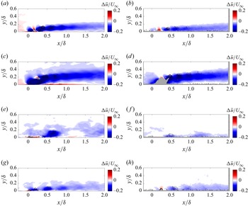


 Open access

