2. Mathematical model

Consider the axisymmetric propagation of a viscous fluid injected into a small gap of height $H$ between two horizontal parallel plates as illustrated in figure 1. From time $t=0$, fluid is injected at a constant volume flux $Q_0$ into the air-filled gap from a small circular hole located on the lower plate. We use a cylindrical coordinate system $(r,\theta,z)$, with the origin chosen to coincide with the position of the centre of the source. At later times, two regions of flow develop: an inner contact region, $0 < r < r_G(t)$, where the fluid is in contact with both plates; and an outer annular region, $r_G(t) < r < r_N(t)$, where the free surface of the fluid $z=h(r,t)$ lies below the upper plate. The velocity components in the $r$ and $z$ directions are denoted by $u(r,z,t)$ and $v(r,z,t)$, respectively, and the fluid pressure is given by $p(r,z,t)$. The radial flux, which is continuous across the two regions, is denoted by $q$. Let $\rho$ be the density of the fluid, and $\nu = \mu /\rho$ the kinematic viscosity, where $\mu$ is the dynamic viscosity.

Figure 1.

Side view of a confined viscous gravity current. Typical velocity profiles in the inner contact region, $0 < r< r_G(t)$ (Region 1), and the annular gravity current region, $r_G(t)< r< r_N(t)$ (Region 2), are shown.

In contrast to the model considered by Hinton (Reference Hinton2020), the displaced air is assumed to be inviscid, which allows for the development of a grounding line separating the inner contact region from the outer annular region. We apply lubrication theory, which is valid once $Re(H/L) \ll 1$, where $Re = U H/\nu$ is the Reynolds number and $L$ is the smaller of the characteristic lengths corresponding to $r_G$ and $r_N - r_G$.

In Region 1, $0< r< r_G(t)$, conservation of mass determines the radial flux $q$ by

(2.1)\begin{equation} 2 {\rm \pi}r q(r) = Q_0. \end{equation}

In Region 2, $r_G(t)< r< r_N(t)$, the flow is that of a classical viscous, free-surface gravity current (Huppert Reference Huppert1982) in which the pressure $p$ relative to atmospheric is

(2.2)\begin{equation} p (r,z,t) = \rho g (h-z), \end{equation}

and the radial velocity

(2.3)\begin{equation} u (r,z,t) = \frac{g}{2 \nu} \frac{\partial h}{\partial r} z (z - 2 h), \end{equation}

satisfies no slip at $z=0$ and no stress at $z=h(r,t)$. The radial flux is given by

(2.4)\begin{equation} q (r,t) \equiv \int_0^h u(r,z,t) dz ={-}\frac{g}{3 \nu} h^3 \frac{\partial h}{\partial r}. \end{equation}

The rate of change of the free-surface height is related to $q$ by the local mass-conservation equation

(2.5)\begin{equation} \frac{\partial h}{\partial t} + \frac{1}{r} \frac{\partial}{\partial r} \left(r q \right) = 0, \end{equation}

which leads to the equation

(2.6)\begin{equation} \frac{\partial h}{\partial t} = \frac{g}{3 \nu} \frac{1}{r} \frac{\partial}{\partial r} \left(r h^3 \frac{\partial h}{\partial r} \right). \end{equation}

At $r=r_G$, the gravity-current solution intersects the upper boundary so

(2.7)\begin{equation} h(r_G(t),t) = H. \end{equation}

Additionally, conservation of mass there gives that

(2.8)\begin{equation} \left.-\frac{g}{3 \nu} h^3 \dfrac{\partial h}{\partial r} \right\rvert_{r_G^+}= \frac{Q_0}{2 {\rm \pi}r_G}. \end{equation}

At the leading edge, $r=r_N$, the height of the free surface is zero,

(2.9)\begin{equation} h(r_N(t),t) = 0, \end{equation}

while global conservation of mass requires that

(2.10)\begin{equation} Q_0 t = {\rm \pi}r_G^2 H + 2 {\rm \pi}\int_{r_G}^{r_N} h r \,{\rm d}r. \end{equation}

Alternatively, we can differentiate (2.10) with respect to time, and use the continuity equation (2.6) with (2.7) and (2.8) to show that

(2.11)\begin{equation} \frac{{\rm d} r_N}{{\rm d} t} = \lim_{r \rightarrow r_N} \dfrac{q}{h} = \lim_{r \rightarrow r_N} \left(-\dfrac{g}{3 \nu} h^2 \dfrac{\partial h}{\partial r} \right), \end{equation}

which is a consequence of imposing zero flux through the leading edge.

2.1. Similarity solutions

Classical unconfined axisymmetric Newtonian viscous gravity currents with a constant flux can be described by similarity solutions in which the radius scales with the square root of time and the height scale is independent of time (Huppert Reference Huppert1982). Radial spreading proportional to the square root of time is also a consequence of mass conservation in two-dimensional flow from a point source. It is therefore anticipated that the introduction of the external vertical length scale is consistent with a similar transformation for flows confined between parallel, horizontal boundaries. We see this by using $H$ to scale $h$ and balancing the terms in (2.6) to give

(2.12)\begin{equation} r \sim \left(\dfrac{g H^3 t}{3 \nu}\right)^{1/2}. \end{equation}

Note that this scaling also balances all three terms in the mass-conservation equation (2.10). We therefore introduce the similarity transformation

(2.13a,b)\begin{equation} h(r,t) = H f(\eta), \quad \eta = \left( \frac{3 \nu}{g H^3 t} \right)^{1/2} r, \end{equation}

with

(2.14a,b)\begin{equation} r_G(t) = \eta_G \left( \frac{g H^3 t}{3 \nu} \right)^{1/2}, \quad r_N(t) = \eta_N \left( \frac{g H^3 t}{3 \nu} \right)^{1/2}, \end{equation}

where $\eta _G$ and $\eta _N$ are constants to be determined. The partial differential equation (2.6) thus reduces to the ODE

(2.15)\begin{equation} (\eta f^3 f' )' + \tfrac{1}{2} \eta^2 f' = 0, \end{equation}

and the boundary conditions (2.7)–(2.9) and (2.11) become

(2.16a,b)\begin{gather} f\left(\eta_G \right) = 1, \quad \eta_G f^3(\eta_G) f'\left(\eta_G \right) ={-}J^4, \end{gather}

(2.17a,b)\begin{gather} f(\eta_N) = 0, \quad \lim_{\eta\to\eta_N} f^2 f' ={-}\tfrac{1}{2} \eta_N, \end{gather}

where

(2.18)\begin{equation} J = \left.\left(\dfrac{3 Q_0 \nu}{2 {\rm \pi}g} \right)^{1/4} \right/H \end{equation}

is the ratio of the scale height for an unconfined gravity current to the gap width of the cell and $'$ denotes derivatives with respect to $\eta$. A similar dimensionless parameter $\varLambda$, which reduces to $\varLambda = J^{4}$ when the density of the ambient fluid is neglected and represents a dimensionless volume flux, was identified by Hinton (Reference Hinton2020). Although (2.15) and the boundary conditions at the leading edge (2.17a,b) apply to unconfined axisymmetric gravity currents, the boundary conditions (2.16a,b) are specific to confined flows. We note that the existence of similarity solutions is a consequence of the coincidence mentioned above given axisymmetric flow of a Newtonian fluid in a horizontal layer of uniform thickness. Different relationships between these control parameters would be required for self-similarity if the fluid were non-Newtonian, for example.

From (2.17a,b), we see that the solution for $f$ at $\eta _N$ is singular. However, an asymptotic solution for $f$ near $\eta _N$ can be used to discern the behaviour there. Setting $\eta = \eta _N$ in (2.15) results in

(2.19)\begin{equation} (f^3 f')' + \tfrac{1}{2} \eta_N f' = 0, \end{equation}

which, solving subject to (2.17a,b), gives

(2.20a,b)\begin{equation} f(\eta) \sim \left( \dfrac{3 \eta_N}{2} \right)^{1/3} (\eta_N - \eta)^{1/3}, \quad f'(\eta) \sim{-} \left( \dfrac{\eta_N}{18} \right)^{1/3} (\eta_N - \eta)^{{-}2/3}. \end{equation}

This asymptotic solution is used to initialise the numerical solution described in § 2.2.

2.2. Numerical results

The second-order ODE (2.15) can be written as a system of first-order ODEs by introducing the variable, $g = \eta f^3 f'$, resulting in

(2.21a,b)\begin{equation} f' = \frac{g}{\eta f^3}, \quad g' ={-} \frac{\eta g}{2 f^3}. \end{equation}

From (2.16a,b) and (2.17a,b), the boundary conditions on $f$ and $g$ are

(2.22a–d)\begin{equation} f(\eta_G) =1, \quad f(\eta_N) = 0, \quad g(\eta_G) ={-}J^4, \quad g(\eta_N)=0. \end{equation}

The routine ODE15s from Matlab R2019a was used to solve (2.21a,b) subject to (2.22a–d) on the domain $[\eta _G, \eta _N-\delta ]$, where $\delta = 10^{-8}$ was chosen such that the solution changed by less than 0.002 % on further reduction of $\delta$. The conditions for $f$ and $g$ at $\eta _N- \delta$,

(2.23a,b)\begin{equation} f(\eta) =\left( \dfrac{3 \eta_N}{2} \right)^{1/3} \delta^{1/3}, \quad g(\eta) ={-}\dfrac{\eta_N}{3} \left( \dfrac{3 \eta_N}{2} \right)^{4/3} \delta^{1/3}, \end{equation}

are obtained from the asymptotic solution in (2.20a,b). We used (2.23a,b) as the initial conditions and integrated backwards along the domain $[\eta _G, \eta _N-\delta ]$, finding the parameter $\eta _G$ from the condition $f(\eta _G)=1$ for a prescribed value of $\eta _N$. The corresponding value of $J$ was then determined from (2.22c) as $J=(-g(\eta _G))^{1/4}$. This implicit relationship allowed us to plot $\eta _G(J)$.

Dimensionless height profiles for various values of $J$ are shown in figure 2, each displaying different qualitative features. For $J=0.25$, the flow is essentially unconfined, the gravity current occupies the majority of the domain, and the inner contact region is negligible. There is a noticeable inflection point near to $\eta _N$ which is a characteristic of unconfined axisymmetric gravity currents. On the other extreme, for $J=2$ the inner contact region fills most of the domain, the gravity current occupies little of the domain, and the flow is essentially described as a Hele-Shaw flow. The height profile for an intermediate value of $J=0.75$ is displayed in figure 2(b) in which both the inner contact region and the gravity current region are well-defined and distinct.

Figure 2.

Typical dimensionless height profiles determined numerically for different values of $J$. For small values of $J$ the flow is essentially unconfined, while for large values of $J$ the flow fills the gap almost completely.

In figure 3(a), the dimensionless front positions, $\eta _G(J)$ and $\eta _N(J)$, are plotted against $J$, and in figure 3(b) the ratio $\eta _G/\eta _N$ is plotted against $J$. We see that for larger values of $J$, $\eta _G \approx \eta _N$ and the inner contact region occupies the majority of the domain. The asymptotic behaviour can be determined by using the expression for $f$ in (2.20) and solving for $\eta _G$ and $\eta _N$ in terms of $J$ by applying the boundary condition $f(\eta _G)=1$ and imposing mass-conservation (2.10). Applying $f(\eta _G)=1$, we find that

(2.24)\begin{equation} \eta_N-\eta_G \sim \frac{2}{3 \eta_N}, \end{equation}

while imposing global mass-conservation gives

(2.25a,b)\begin{align} 2 J^4 &\sim \eta_G^2 + 2 \int_{\eta_G}^{\eta_N} \eta \left( \dfrac{3 \eta_N}{2} \right)^{1/3} (\eta_N - \eta)^{1/3} \,{\rm d} \eta \nonumber\\ &\sim \eta_G^2 +2 \eta_N \left( \dfrac{3 \eta_N}{2} \right)^{1/3} \int_{\eta_G}^{\eta_N} (\eta_N - \eta)^{1/3} \,{\rm d} \eta \end{align}

to leading order in $\eta _N-\eta _G$. The latter integral in (2.25) is readily calculated and combined with (2.24) to show that

(2.26)\begin{equation} 2 J^4 \sim \eta_G^2 + 1. \end{equation}

From (2.24) and (2.26), we obtain

(2.27)\begin{equation} \eta_G \sim \sqrt{2} J^2\left( 1 - \frac{1}{4 J^4} \right), \quad \eta_N \sim \sqrt{2} J^2 \left( 1 + \frac{1}{12 J^4} \right), \end{equation}

and

(2.28)\begin{equation} \frac{\eta_G}{\eta_N} \sim 1 -\frac{1}{3 J^4} \end{equation}

to first order when $J \gg 1$. The leading-order result $\eta _G \sim \eta _N \sim \sqrt {2} J^2$ is straightforwardly understood from conservation of mass in the Hele-Shaw limit. These asymptotic results are seen in figure 3 to give very good representations of the numerical solution once $J \gtrsim 1$. Although there is no grounding line in Hinton's model (Hinton Reference Hinton2020), we can compare the position of the leading edge when the viscosity ratio between the injected fluid and the ambient fluid $M$ tends to infinity. The leading-order position of the leading edge $\eta _N$ given in figure 6 of Hinton (Reference Hinton2020) for $M=100$ is very close to the value given above, which is to be expected because there will be little ambient fluid remaining in the squeeze film when $M$ is large.

Figure 3.

Numerical solutions (black curves) for $\eta _G$ and $\eta _N$ against $J$ (a) and their ratio (b). The associated asymptotic solutions for $J \ll 1$, (2.29) and (2.32), and $J \gg 1$, (2.27) and (2.28), are shown with red, dashed curves. The different flow regimes and the transition regions are shown in (b), while in (a) the value $J=0.78$ corresponds to the largest value of $J$ for which the height profiles contain a point of inflection.

For small values of $J$, the gravity current is essentially unconfined and the similarity solution derived by Huppert (Reference Huppert1982) applies. This can be reproduced here by scaling $f$ with $J$ and $\eta$ by $J^{3/2}$ and then solving the scaled version of (2.21a,b) using the boundary conditions $\eta _G=0$ and the rescaled $g \rightarrow -1$ as $\eta \rightarrow 0$. With this approach, our calculations give

(2.29)\begin{equation} \eta_N \sim 1.42 J^{3/2} \end{equation}

to leading order, which is equivalent to the results given by Huppert (Reference Huppert1982) and Hinton (Reference Hinton2020). This asymptotic solution is seen in figure 3(a) to agree very closely with the numerical solutions for $J \lesssim 0.75$.

We anticipate that $\eta _G \ll 1$ when $J \ll 1$, which is portrayed in figure 3(a). Therefore, in the neighbourhood of $\eta _G$, the second term in (2.15) is negligible and the equation can then readily be integrated using boundary conditions (2.16a,b) to give

(2.30)\begin{equation} f \sim \left[1 - 4 J^4 \ln\left(\frac{\eta}{\eta_G}\right)\right]^{1/4}. \end{equation}

We know from scaling that for most of the unconfined current $f = O(J)$ while $\eta = O(J^{3/2})$. Therefore,

(2.31)\begin{equation} \eta_G \sim \xi J^{3/2} e^{{-}1/(4J^4)} \end{equation}

for some constant $\xi$. It is noteworthy that the asymptotic solution (2.30) has the property that $f=0$ at some finite value of $\eta$ and, if we arbitrarily set that value of $\eta$ to be $\eta _N$, we obtain the result

(2.32)\begin{equation} \eta_G \sim \eta_N e^{{-}1/(4J^4)} \end{equation}

which coincides with (2.31) with $\xi \simeq 1.42$. We have not been able to prove this result asymptotically but find that it gives excellent agreement with our numerical results, as shown in figure 3. Actually, the coefficient $\xi$ is of minor significance relative to the functional form of (2.31), which shows that $\eta _G$ behaves in an Arrhenius fashion with $J$ (cf. detonation phenomena) with extremely rapid growth away from zero at a finite value of $J$. Any reasonable estimate for $\eta _G$ being significantly above zero (e.g. $\eta _G/\eta _N = 1\,\%$ or 5 %) gives a transition value of $J \approx 0.5$. This rapid, exponential transition from an unconfined gravity current to a confined current contrasts with the much slower, algebraic transition from confined gravity current to Hele-Shaw flow shown by (2.28) and the shaded regions in figure 3(b).

From figure 3(b), we see that for $J \leq 0.48$, $\eta _G/\eta _N \le 0.01$, and the gravity current, which occupies more than 99 % of the domain, is essentially unconfined. For $J \geq 2.40$, $\eta _G/\eta _N \geq 0.99$, and the inner contact region occupies 99 % of the domain, which corresponds to the Hele-Shaw limit. Confined gravity currents form in the interval $0.54 \leq J \leq 1.59$, where the inner contact region occupies between 5 % to 95 % of the domain. Within this region, there is a slight shift in behaviour at $J=0.78$. For $J < 0.78$, the height profiles contain a point of inflection as shown in figure 2(a), whereas for $J>0.78$ there is no inflection point.

3. Comparison with experiments

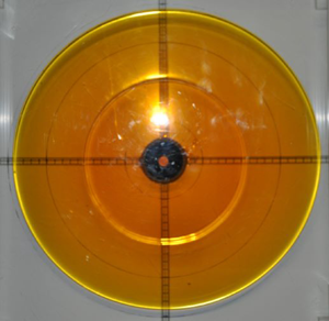
We performed a series of 27 experiments in which golden syrup was injected into the narrow gap between two Perspex sheets from a circular hole in the centre of the lower sheet. A schematic diagram of the set-up in shown in figure 4. The length of each side of the top square sheet was 50 cm and the hole in the lower sheet had a diameter of $5.5$ cm. Three different gap sizes were investigated for fluxes ranging from 0.06–18 cm$^3$ s$^{-1}$. Small square plate spacings were positioned at each of the four corners to support the top sheet. A major consideration in the experimental set-up was the thickness of the top and bottom Perspex sheets, chosen to minimise deflection. The sheets were 1.5 cm thick and were clamped along opposite edges. Given the Young's modulus of Perspex (5.6 GPa), we estimate that these measures ensured that any deflection resulting from the weight of each sheet and the pressure from the fluid that comes into contact with them during an experiment was less than 40 $\mu$m in the most extreme experiment. Vernier callipers were used to measure the gap spacing at each of the four corners and at different positions along the outer edges when the top sheet was clamped down firmly. The measured gap spacings were $(0.71 \pm 0.02)$ cm, $(1.07 \pm 0.02)$ cm and $(1.48 \pm 0.02)$ cm. Out of 27 experiments, seven of them were unconfined viscous gravity currents in which the fluid interface did not intersect with the top sheet within the time scale of the experiment. The remaining experiments exhibited confined viscous gravity current behaviour where the inner contact region and the gravity current region were both well-defined, as shown in figure 5(a).

Figure 4.

Schematic diagram of the side view of the experimental set-up drawn approximately to scale showing the delivery system and the narrow gap between two Perspex sheets into which golden syrup is injected.

Figure 5.

Sample photograph of a confined viscous gravity current viewed from above for an experiment with $J=0.63$ (a). Plot of data points for $r_G^2$ and $r_N^2$ as well as their linear regressions (b).

The fluid delivery system consisted of a mechanical traverse-driven pump which was used to ensure that the fluid flux remained constant throughout the duration of each experiment. The pump consisted of a vertical cylindrical tube of diameter 19 cm and height 52 cm with a fitted pipe at the bottom end where the fluid is released, and a movable close-fitting piston inside the tube driven by a stepper motor. Inside the cylindrical tube, syrup was contained in a collapsible bag that fed the fluid into the fitted pipe at the bottom end of the tube. Large-diameter pipes were used in the delivery system to reduce viscous resistance and allow the pump to maintain a constant volume flux reliably. The initial position of the piston was set so that it was in direct contact with the top of the sealed end of the bag and that the syrup in the sealed bag expanded to reach the walls of the cylindrical tube. The two input parameters to the controller for the stepper motor were the speed at which the piston is driven downwards, which controls the output flux, and the distance the piston must traverse, which corresponds to the total volume of fluid released.

The relationship between the nominal pump speed $S$ (mm s$^{-1}$) and the output flux $Q$ (cm$^3$ s$^{-1}$) was derived by running a series of Hele-Shaw flow experiments at different piston speeds, and then calculating the volume at various times from the experimental images. A graph of volume versus time was plotted, and the gradient, which is equivalent to the flux, was found for each piston speed. A total of six experiments were used to derive the constant of proportionality between the pump speed and the output flux. The flux values for each experiment are shown in table 1.

Table 1.

Experimental input values, which are temperature, kinematic viscosity, gap spacing, and volume flux, along with the corresponding $J$ values found from (2.18). The results for $\alpha _G$ and $\alpha _N$ found from the linear regressions (3.1a,b) as well as $\eta _G$, $\eta _N$ and $\eta _G/\eta _N$ obtained from the relationships in (3.2a,b) are displayed. The maximum errors corresponding to each parameter are shown in the third row. The errors shown for $\eta _G$, $\eta _N$, and $\eta _G/\eta _N$ are based on the error estimates reported in earlier columns.

The density of the syrup was measured to be $(1421 \pm 15)$ kg m$^{-3}$. Because the viscosity of syrup is highly dependent on temperature $T$, the temperature of the syrup was recorded before each experiment, and was found to lie in the range 19–21 $^{\circ }$C. Using a viscometer, we found that at 22 $^{\circ }$C and 23.5 $^{\circ }$C the dynamic viscosity of the Lyle's golden syrup that we used was $(37.6 \pm 1.2)$ Pa s and $(30.3 \pm 1.2)$ Pa s, respectively. In order to estimate the viscosity at lower temperatures in the range 19–21 $^{\circ }$C, we first extracted the data set showing dynamic viscosity $\mu$ as a function of temperature $T$ for Lyle's golden syrup as presented by Beckett et al. (Reference Beckett, Mader, Phillips, Rust and Witham2011) and then applied a curve of the form $\mu = A \exp (-B T)$ to the data set with $T$ measured in Celsius. We found that a best fit gave $A=1470$ Pa s and $B=0.15\,^{\circ }{\rm C}^{-1}$. Using our experimental values, we obtained $\mu = A \exp (-0.15 T)$ where $A=1023$ Pa s. The kinematic viscosity at temperatures 19 $^{\circ }$C, 20 $^{\circ }$C, 21 $^{\circ }$C were then calculated to be (420 $\pm$ 30) cm$^2$ s$^{-1}$, (360 $\pm$ 30) cm$^2$ s$^{-1}$ and (310 $\pm$ 30) cm$^2$ s$^{-1}$, respectively. The error corresponds to an uncertainty in temperature of 0.5 $^{\circ }$C. The largest source of uncertainty in these experiments was associated with viscosity variations.

From photographs of the experiments such as that shown in figure 5(a), the mean radius of the inner region $r_G(t)$ and of the outer region $r_N(t)$ were calculated from the areas of ellipses fitted by eye using tools in ImageJ (Schneider, Rasband & Eliceiri Reference Schneider, Rasband and Eliceiri2012) as radius $=$ (area/${\rm \pi}$)$^{1/2}$. For each data set, we used linear regressions to determine coefficients $\alpha _G$ and $\alpha _N$ such that

(3.1a,b)\begin{equation} r_G^2(t) = \alpha_G^2 t, \quad r_N^2(t) = \alpha_N^2 t, \end{equation}

as shown in figure 5(b). To reduce the influence of initial transients, some early-time data points were omitted from the regression. From (2.14a,b),

(3.2a,b)\begin{equation} \eta_G = \alpha_G \left( \frac{3 \nu}{g H^3 } \right)^{1/2}, \quad \eta_N =\alpha_N \left( \frac{3 \nu}{g H^3 } \right)^{1/2}. \end{equation}

The parameters for each experiment and our principal measurements are given in table 1.

In figure 6, the data points $(J,\eta _G)$ and $(J,\eta _N)$ are displayed along with the theoretical curves obtained in § 2. The data points $\square$, $\circ$ and $\diamond$ correspond to gap spacings 0.71 cm, 1.48 cm and 1.07 cm, respectively.

Figure 6.

Data points $(J,\eta _G)$ (filled-in shapes) and $(J,\eta _N)$ (open shapes), where $\square$, $\circ$ and $\diamond$ correspond to gap spacings 0.71 cm, 1.48 cm and 1.07 cm, respectively, along with the theoretical curves (a). Data points $(J,\eta _G/\eta _N)$ (filled-in shapes) along with the theoretical curve (b).

Overall, we see that our scaling analysis and corresponding similarity theory capture the dominant variations of $\eta _G$ and $\eta _N$ with $J$ very well. There is generally good agreement between our experimental results for $\eta _N$, shown by the open symbols in figure 6(a), and the corresponding theoretical predictions, particularly given experimental uncertainty, indicated with representative error bars on the right-most data points. There is also reasonable agreement between theory and experiment for the position of the contact line $\eta _N$ separating the contact region from the gravity current. Here, however, we see some systematic variation of $\eta _G$ with gap spacing, with the experimental values of $\eta _G$ corresponding to similar values of $J$ decreasing slightly as the gap spacing increases. Such systematic deviation from the similarity solution and the lack of a complete collapse of the data onto a universal curve given by our scaling suggests the influence of additional physics not included in our model, which we discuss in § 4. We note particularly the increasing deviation of the experimental results and the theoretical predictions as $J$ approaches the values required for essentially unconfined gravity currents from above.

These trends are amplified by considering the ratio $\eta _G/\eta _N$, shown in figure 6(b), where we see, nevertheless, that our theory captures the dominant, gradual transition between confined gravity currents and Hele-Shaw flows at values of $J$ around unity very well. A strong result of this study is the rapid transition from essentially unconfined gravity currents to confined currents at values of $J\approx 0.5$ (cf. figures 3b and 6b). We note that the similarity solution for an axisymmetric gravity current from a point source has a logarithmic singularity at the origin that makes $\eta _G$ formally non-zero for any non-zero value of $J$, while laboratory experiments from a finite source allows the current not to make contact with the top plate at all. It is possible that an experiment run for a very long time would eventually have the current make contact with the top plate. However, within the finite time of our experiments, we found that there was no contact for $J<0.48$ and contact for $J>0.53$. This compares very favourably with our theoretical predictions that the transition $0.01 < \eta _G/\eta _N < 0.05$ occurs in the range $0.48 < J < 0.54$. Although the annular region was too small for the thin-film approximation to be valid, we show with a pink triangle in figure 6(b) the ratio of $r_G/r_N$ for one of the calibration experiments, which coincides with the theoretical curve extremely well.