





1. Introduction
When acoustic fields are applied to fluids, they induce steady fluid motions known as acoustic streaming (Rayleigh Reference Rayleigh1884; Nyborg Reference Nyborg1958; Lighthill Reference Lighthill1978), and generate radiation forces (King Reference King1934; Yosioka & Kawasima Reference Yosioka and Kawasima1955; Gor’kov Reference Gor’kov1962; Toftul et al. Reference Toftul, Bliokh, Petrov and Nori2019) due to the scattering of acoustic waves on suspended particles. These phenomena, especially at microscales, constitute the field of acoustofluidics, and are pivotal in various applications, such as particle or cell sorting (Nilsson et al. Reference Nilsson, Petersson, Jönsson and Laurell2004; Laurell, Petersson & Nilsson Reference Laurell, Petersson and Nilsson2007; Gedge & Hill Reference Gedge and Hill2012; Jakobsson et al. Reference Jakobsson, Grenvall, Nordin, Evander and Laurell2014; Fornell et al. Reference Fornell, Nilsson, Jonsson, Periyannan Rajeswari, Joensson and Tenje2015; Lenshof et al. Reference Lenshof, Johannesson, Evander, Nilsson and Laurell2017; Wu et al. Reference Wu, Ozcelik, Rufo, Wang, Fang and Jun Huang2019; Das & Bhethanabotla Reference Das and Bhethanabotla2022), fluid mixing (Yeo & Friend Reference Yeo and Friend2014; Ozcelik et al. Reference Ozcelik, Rufo, Guo, Gu, Li, Lata and Huang2018; Das, Snider & Bhethanabotla Reference Das, Snider and Bhethanabotla2020; Huang, Das & Bhethanabotla Reference Huang, Das and Bhethanabotla2021) and trapping of particles (Nilsson et al. Reference Nilsson, Evander, Hammarström and Laurell2009; Evander & Nilsson Reference Evander and Nilsson2012).
The utilisation of droplets or bubbles suspended in an immiscible fluid medium under ultrasonic fields is a key aspect of acoustofluidics. These two-phase acoustofluidic systems are highly versatile and find applications in areas such as particle manipulations (Fornell et al. Reference Fornell, Garofalo, Nilsson, Bruus and Tenje2018; Shi et al. Reference Shi, Baasch, Liu, Fornell, Werr, Barbe and Tenje2025), micro-robotic actuations (Dijkink et al. Reference Dijkink, van der Dennen, Ohl and Prosperetti2006; Ahmed et al. Reference Ahmed, Lu, Nourhani, Lammert, Stratton, Muddana, Crespi and Huang2015; Celik Cogal et al. Reference Celik Cogal, Das, Yurdabak Karaca, Bhethanabotla and Uygun Oksuz2021 a; Mohanty et al. Reference Mohanty, Lin, Paul, van den Broek, Segers and Misra2024; Das et al. Reference Das, Cogal, Oksuz and Bhethanabotla2025), acoustic levitation (Yarin, Pfaffenlehner & Tropea Reference Yarin, Pfaffenlehner and Tropea1998; Zang et al. Reference Zang, Yu, Chen, Li, Wu and Geng2017, Reference Zang, Li, Di, Zhang, Ding, Chen, Shen, Binks and Geng2018; Di et al. Reference Di, Zhang, Li, Lin, Li, Li, Binks, Chen and Zang2018), drug delivery (Coussios & Roy Reference Coussios and Roy2008; Ho et al. Reference Ho, Wu, Hsieh, Fan and Yeh2018; Celik Cogal et al. Reference Celik Cogal, Das, Yurdabak Karaca, Bhethanabotla and Uygun Oksuz2021b ; Janiak et al. Reference Janiak, Li, Ferry, Doinikov and Ahmed2023; Shakya et al. Reference Shakya, Cattaneo, Guerriero, Prasanna, Fiorini and Supponen2024), 3D printing (Jin et al. Reference Jin, Wei, Yu, Ren, Meng and Jiang2020; Habibi et al. Reference Habibi, Foroughi, Karamzadeh and Packirisamy2022; Derayatifar et al. Reference Derayatifar, Habibi, Bhat and Packirisamy2024; Vidler et al. Reference Vidler2024), oil recovery from water–oil emulsions (Adeyemi et al. Reference Adeyemi, Meribout, Khezzar, Kharoua and AlHammadi2022) or as ‘miniaturised systems’ for various biomedical tests such as cell culturing (Hensel, Mienkina & Schmitz Reference Hensel, Mienkina and Schmitz2011; Fornell et al. Reference Fornell, Johannesson, Searle, Happstadius, Nilsson and Tenje2019, Reference Fornell, Pohlit, Shi and Tenje2021; Ali et al. Reference Ali, Lee, Cha, Kim, Oyunbaatar, Lee and Park2024), single-cell analysis (Gerlt et al. Reference Gerlt, Haidas, Ratschat, Suter, Dittrich and Dual2020; Lee et al. Reference Lee, Tang, Chen, Zhong and Kim2024) or studying cell-to-cell interactions (Guo et al. Reference Guo, Li, French, Mao, Zhao, Li, Nama, Fick, Benkovic and Huang2015). The interaction between ultrasonic fields and viscous droplets induces strong oscillations at the droplet surface, giving rise to acoustic streaming both within and around the droplet. This streaming, combined with the acoustic radiation forces, triggers significant deformations, altering the droplet’s shape and modifying its internal flow patterns (Cheung, Nguyen & Wong Reference Cheung, Nguyen and Wong2014; Lu et al. Reference Lu, Twiefel, Ma, Yu, Wallaschek and Fischer2021). The nature of this interaction critically depends on the relation between the acoustic frequency and the droplet’s capillary eigenfrequencies. A substantial body of work addresses capillary-resonant excitation of free droplets (Marston Reference Marston1980; Yarin Reference Yarin2001; Spelman & Lauga Reference Spelman and Lauga2017), demonstrating that, near resonance, the amplitudes of individual shape modes grow strongly, nonlinear mode coupling becomes important and the resulting streaming and mean-shape evolution can differ qualitatively from non-resonant predictions. These capillary-resonant phenomena represent an important counterpart to acoustofluidic droplet dynamics and highlight the need for unified theoretical frameworks bridging acoustically forced and capillary-resonant regimes. Although the present study focuses on classical acoustic streaming (Rayleigh Reference Rayleigh1884; Nyborg Reference Nyborg1953; Lighthill Reference Lighthill1978), for which capillary-mode amplification is negligible, we have outlined the relevant literature to situate our work within the broader context of acoustic–droplet interactions. In bubble microfluidics, recent studies have explicitly connected acoustofluidic formulations with capillary-driven bubble-dynamics models (Agarwal et al. Reference Agarwal, Upadhyay, Bhosale, Gazzola and Hilgenfeldt2024), and analogous unifying perspectives are now emerging in droplet microfluidics. Together, these developments emphasise that acoustically driven flows, interfacial oscillations and capillary dynamics are often intertwined and should be interpreted within a common physical framework.
The pioneering work on acoustic streaming around bubbles began with the experimental studies of Kolb & Nyborg (Reference Kolb and Nyborg1956), who first identified vortex motions in the vicinity of solid surfaces or small oscillating microbubbles. This initial discovery sparked further investigations, notably by Elder (Reference Elder1959), who explored cavitation microstreaming and observed various flow patterns that intrigued theoretical interest. Building on these observations, Davidson & Riley (Reference Davidson and Riley1971) utilised perturbation theory to model bubble-induced streaming by treating the bubble as a fixed-shape oscillator in an incompressible fluid. Subsequently, numerous experimental and theoretical investigations have been conducted to elucidate the streaming flows induced by single and multiple bubble systems, both in proximity to solid boundaries and in unbounded fluid domains (Wu & Du Reference Wu and Du1997; Longuet-Higgins Reference Longuet-Higgins1998; Zhao et al. Reference Zhao, Sadhal and Trinh1999b
; Marmottant et al. Reference Marmottant, Raven, Gardeniers, Bomer and Hilgenfeldt2006; Tho, Manasseh & Ooi Reference Tho, Manasseh and Ooi2007; Ahmed et al. Reference Ahmed, Mao, Shi, Juluri and Huang2009; Doinikov & Bouakaz Reference Doinikov and Bouakaz2010). The role of higher-order surface modes has also received attention, with studies showing that each mode of order $n$
produces a characteristic
$n$
produces a characteristic $2n$
-lobed streaming structure around the bubble (Cleve et al. Reference Cleve, Guédra, Mauger, Inserra and Blanc-Benon2019). More recent experiments show that non-spherical or parametrically driven modes can dominate the streaming field, indicating that constant-frequency, purely linear models are insufficient to describe bubble-induced microstreaming under strong excitation (Guédra et al. Reference Guédra, Cleve, Mauger and Inserra2020), consistent with existing theoretical predictions (Longuet-Higgins Reference Longuet-Higgins1989). Despite this progress, most classical analyses have predominantly focused on capturing the external streaming phenomena occurring outside the bubbles, with comparatively little attention paid to the internal acoustic streaming. Notable exceptions are the models of Wu & Du (Reference Wu and Du1997) and Doinikov & Bouakaz (Reference Doinikov and Bouakaz2010), which provide unified formulations for both internal and external flow fields. The model of Wu & Du (Reference Wu and Du1997) operates under the assumption that the viscous boundary layer is significantly thinner than the bubble diameter, simplifying the bulk fluid as inviscid, thus restricting its applicability to low-viscosity fluids only. To address these limitations, Doinikov & Bouakaz developed a more comprehensive model, integrating viscous and thermal effects in heat-conducting fluids, thereby offering a generalised solution for streaming both inside and outside oscillating spherical bubbles.
$2n$
-lobed streaming structure around the bubble (Cleve et al. Reference Cleve, Guédra, Mauger, Inserra and Blanc-Benon2019). More recent experiments show that non-spherical or parametrically driven modes can dominate the streaming field, indicating that constant-frequency, purely linear models are insufficient to describe bubble-induced microstreaming under strong excitation (Guédra et al. Reference Guédra, Cleve, Mauger and Inserra2020), consistent with existing theoretical predictions (Longuet-Higgins Reference Longuet-Higgins1989). Despite this progress, most classical analyses have predominantly focused on capturing the external streaming phenomena occurring outside the bubbles, with comparatively little attention paid to the internal acoustic streaming. Notable exceptions are the models of Wu & Du (Reference Wu and Du1997) and Doinikov & Bouakaz (Reference Doinikov and Bouakaz2010), which provide unified formulations for both internal and external flow fields. The model of Wu & Du (Reference Wu and Du1997) operates under the assumption that the viscous boundary layer is significantly thinner than the bubble diameter, simplifying the bulk fluid as inviscid, thus restricting its applicability to low-viscosity fluids only. To address these limitations, Doinikov & Bouakaz developed a more comprehensive model, integrating viscous and thermal effects in heat-conducting fluids, thereby offering a generalised solution for streaming both inside and outside oscillating spherical bubbles.
While the above literature predominantly explored scenarios involving bubbles submerged in liquid media, the inverse case where droplets are suspended in a gaseous environment under ultrasound excitation has also garnered significant research interest. One of the pioneering experiments in this domain was conducted by Trinh (Reference Trinh1985), who investigated ultrasound-induced capillary-resonant oscillations in microgravity to enable contactless acoustic levitation. Subsequently, Trinh & Robey (Reference Trinh and Robey1994) expanded on this work, experimentally demonstrating acoustic streaming around a levitated droplet suspended in gas. They identified the onset of flow instability due to localised heating at the levitation spot, which disrupted the resonance conditions necessary for stable levitation. Further theoretical advancements were made by Zhao et al. (Reference Zhao, Sadhal and Trinh1999a ) and Rednikov et al. (Reference Rednikov, Zhao, Sadhal and Trinh2006), who developed analytical models for the acoustic-streaming flow both inside the levitated droplet and in the surrounding gas. Their analysis revealed the cessation of internal recirculation within the Stokes boundary layer for specific frequency ranges and particular liquid-to-gas viscosity ratios. Building on this, Lee, Sadhal & Rednikov (Reference Lee, Sadhal and Rednikov2008) later investigated the streaming patterns of a levitated, flattened liquid droplet in a gaseous environment. However, these analytical models assumed the droplet maintained a rigid shape, thereby neglecting potential deformations caused by acoustic streaming and radiation forces. This simplification limits the applicability of the results to scenarios where the droplet shape dynamics significantly influences the streaming behaviour.
Within this broader context, ranging from acoustically driven and capillary-resonant droplet oscillations to well-studied bubble dynamics, the streaming and the dynamics of a viscous droplet immersed in a viscous carrier fluid under acoustic excitation remain comparatively underexplored. Early experiments by Trinh, Zwern & Wang (Reference Trinh, Zwern and Wang1982) revealed a rich spectrum of capillary-resonant shape modes and associated internal circulation in liquid droplets subjected to low-amplitude acoustic fields, yet notably reported no persistent steady deformation. In contrast, more recent studies by Cheung et al. (Reference Cheung, Nguyen and Wong2014), Baasch, Doinikov & Dual (Reference Baasch, Doinikov and Dual2020) and Sustiel & Grier (Reference Sustiel and Grier2024) have started to address classical acoustic streaming in two-phase droplet systems. Cheung et al. (Reference Cheung, Nguyen and Wong2014) examined the influence of interfacial tension, acoustic frequency and applied voltage on the dynamics of droplets, focusing on motion, shape deformation and internal streaming within a microfluidic chamber. Theoretical investigations, however, are scarce and have only recently begun to emerge. Baasch et al. (Reference Baasch, Doinikov and Dual2020) developed a model incorporating Stokes drift inside and outside droplets but assumed rigid spheres and considered only monopole and dipole oscillations, omitting higher-order modes relevant for droplets displaced from pressure nodes. More recently, Sustiel & Grier (Reference Sustiel and Grier2024) introduced a hybrid immersed boundary approach for acoustically levitated droplets, yet it neglects the acoustic boundary layer and Stokes drift, is limited to droplets much smaller than the acoustic wavelength and explores only surface-tension variations. Despite these efforts, a unified framework capturing both streaming and shape deformation in viscous–viscous droplet systems is still missing, motivating the present study.
In the Rayleigh regime, where droplet or particle diameters are much smaller than the acoustic wavelength, the incident field is effectively uniform across the object’s surface. Under these conditions, deformation is negligible, and acoustic radiation forces remain weak, primarily governed by the spatial gradient of the Gor’kov potential. Particles or droplets below a critical size are predominantly advected by acoustic streaming, whereas those exceeding this threshold tend to migrate toward stable equilibrium positions, typically at pressure node (PN) or velocity node (VN), depending on their acoustic contrast factor. However, these classical migration laws are not generally valid in the Mie regime. As demonstrated by Pazos Ospina et al. (Reference Pazos Ospina, Contreras, Estrada-Morales, Baresch, Ealo and Volke-Sepúlveda2022), for particle-to-wavelength ratios below 0.6, particles follow the expected migration toward PN or VN, whereas for ratios between 0.6 and 1.0, reversed behaviour and off-axis trapping can occur.
In this work, we focus on droplets within the sub-resonant limit whose sizes exceed the critical threshold for acoustic streaming-dominated droplet transport but remain below the half-wavelength limit, ensuring structural integrity while enabling significant acoustic interaction. In this regime, radiation forces enable precise manipulation without fragmentation, making droplets well suited for biomedical applications requiring robust positional control and enhanced force transduction, including cell encapsulation, tissue engineering and targeted drug delivery. Within this parameter space, spanning the Rayleigh to Mie scattering regimes, we specifically investigate the deformation dynamics analogous to the Taylor regime (Taylor Reference Taylor1934), characterised by axisymmetric shape evolution under defined acoustic flow fields. To capture this dynamics, we develop a comprehensive theoretical framework using multiple-time-scale analysis, yielding both analytical and numerical solutions for the coupled acoustic field and droplet deformation behaviour. This framework effectively captures the essential physics, enabling the identification of distinct acoustic streaming and deformation regimes, along with the key parameters controlling them. Our study reveals that, while acoustic fields are strongly governed by the lower-order oscillation modes (monopole, dipole or quadrupole based on the droplet position), the resulting streaming patterns and droplet mean deformations are strongly governed primarily by the density or compressibility contrasts between the droplet and the surrounding fluid.
Problem definition. (a) A spherical viscous droplet of undeformed radius $R_0$
, density
$R_0$
, density $\rho _-$
, shear viscosity
$\rho _-$
, shear viscosity $\mu _-$
, bulk viscosity
$\mu _-$
, bulk viscosity $\mu _{b-}$
and sound speed
$\mu _{b-}$
and sound speed $c_-$
is suspended in an immiscible surrounding fluid with properties
$c_-$
is suspended in an immiscible surrounding fluid with properties $\rho _+$
,
$\rho _+$
, $\mu _+$
,
$\mu _+$
, $\mu _{b+}$
and
$\mu _{b+}$
and $c_+$
, respectively. The system is subjected to an axisymmetric ultrasonic standing-wave field. Spherical coordinates
$c_+$
, respectively. The system is subjected to an axisymmetric ultrasonic standing-wave field. Spherical coordinates $(r,\theta ,\phi )$
and cylindrical coordinates
$(r,\theta ,\phi )$
and cylindrical coordinates $(z,\eta ,\phi )$
are used to describe the geometry and field variables. (b) Due to the symmetry of the acoustic field about the droplet equator, as considered in this study, only even modes of Legendre polynomial contribute to the droplet shape. The dominant modes
$(z,\eta ,\phi )$
are used to describe the geometry and field variables. (b) Due to the symmetry of the acoustic field about the droplet equator, as considered in this study, only even modes of Legendre polynomial contribute to the droplet shape. The dominant modes $l=0$
,
$l=0$
, $l=2$
and
$l=2$
and $l=4$
are illustrated here.
$l=4$
are illustrated here.

2. Mathematical formulations
2.1. System description
We consider a viscous Newtonian droplet with initial spherical shape having radius $R_0$
, density
$R_0$
, density $\rho _-$
, shear viscosity
$\rho _-$
, shear viscosity $\mu _-$
and bulk viscosity
$\mu _-$
and bulk viscosity $\mu _{b-}$
, suspended in an immiscible Newtonian fluid medium with density
$\mu _{b-}$
, suspended in an immiscible Newtonian fluid medium with density $\rho _+$
, shear viscosity
$\rho _+$
, shear viscosity $\mu _+$
and bulk viscosity
$\mu _+$
and bulk viscosity $\mu _{b+}$
, as shown in figure 1(a). The sonic speeds in the droplet and the continuous medium are
$\mu _{b+}$
, as shown in figure 1(a). The sonic speeds in the droplet and the continuous medium are $c_-$
and
$c_-$
and $c_+$
, respectively. Here, subscripts ‘
$c_+$
, respectively. Here, subscripts ‘ $-$
’ and ‘
$-$
’ and ‘ $+$
’ denote the properties of the droplet and the external continuous medium, respectively. The surface tension at the interface between the two fluids is given by
$+$
’ denote the properties of the droplet and the external continuous medium, respectively. The surface tension at the interface between the two fluids is given by $\gamma$
. The droplet domain is defined as
$\gamma$
. The droplet domain is defined as $\varOmega _-$
, the surrounding medium as
$\varOmega _-$
, the surrounding medium as $\varOmega _+$
and the interface separating them as
$\varOmega _+$
and the interface separating them as $\partial \varOmega$
. The spatial coordinates are described by
$\partial \varOmega$
. The spatial coordinates are described by $\boldsymbol{r} = \boldsymbol{r}(\eta , z, \varphi )$
in a cylindrical coordinate system. The undeformed droplet is assumed to be centred at the origin, i.e.
$\boldsymbol{r} = \boldsymbol{r}(\eta , z, \varphi )$
in a cylindrical coordinate system. The undeformed droplet is assumed to be centred at the origin, i.e. $(\eta ,z)=(0,0)$
, and is subjected to a standing acoustic wave along the
$(\eta ,z)=(0,0)$
, and is subjected to a standing acoustic wave along the $z$
-axis. In the present study, we consider droplets located only at equilibrium positions of the standing acoustic field, namely either PN or VN. The stable equilibrium position depends on the acoustic contrast factor
$z$
-axis. In the present study, we consider droplets located only at equilibrium positions of the standing acoustic field, namely either PN or VN. The stable equilibrium position depends on the acoustic contrast factor $\varPhi$
: droplets with
$\varPhi$
: droplets with ${\varPhi }\gt 0$
are stably located at PN, whereas droplets with
${\varPhi }\gt 0$
are stably located at PN, whereas droplets with ${\varPhi }\lt 0$
are stably located at VN. The complementary position in each case is unstable and is therefore not considered here. The background pressure field in the continuous phase is given by
${\varPhi }\lt 0$
are stably located at VN. The complementary position in each case is unstable and is therefore not considered here. The background pressure field in the continuous phase is given by
 \begin{equation} p_{\textit{bg}}(z, t) = \frac {p_a}{2} \left [ e^{i k_+ (z + d)} + e^{-i k_+ (z + d)} \right ] e^{-i \omega t}, \quad \text{for } \boldsymbol{r} \in \varOmega _+, \end{equation}
where $p_a$
is the pressure amplitude, and
$p_a$
is the pressure amplitude, and $k_+$
is the wavenumber of the acoustic field in the continuous phase. The parameter
$k_+$
is the wavenumber of the acoustic field in the continuous phase. The parameter $d$
specifies the location of the droplet centre relative to the standing wave:
$d$
specifies the location of the droplet centre relative to the standing wave: $k_+d=0$
places the droplet at VN, while
$k_+d=0$
places the droplet at VN, while $k_+d=\pm \pi /2$
places it at PN. These are the only droplet positions considered in the present analysis.
$k_+d=\pm \pi /2$
places it at PN. These are the only droplet positions considered in the present analysis.
The scalar acoustic velocity potential associated with the standing wave is given by
 \begin{equation} \phi _{\textit{bg}} = \frac {\phi _0}{2} \left [ e^{i k_+ (z + d)} + e^{-i k_+ (z + d)} \right ] e^{-i \omega t}, \qquad \boldsymbol{r} \in \varOmega _+, \end{equation}
where $\phi _0 = ({p_a}/{i \rho _{+0} \omega })$
is the amplitude of the velocity potential,
$\phi _0 = ({p_a}/{i \rho _{+0} \omega })$
is the amplitude of the velocity potential, $\omega$
is the angular frequency of the acoustic field and
$\omega$
is the angular frequency of the acoustic field and $\rho _{+0}$
denotes the equilibrium density of the continuous medium in the absence of acoustic excitation. The background acoustic velocity
$\rho _{+0}$
denotes the equilibrium density of the continuous medium in the absence of acoustic excitation. The background acoustic velocity $\boldsymbol{v}_{\textit{bg}}$
is related to the scalar potential via
$\boldsymbol{v}_{\textit{bg}}$
is related to the scalar potential via $\boldsymbol{v}_{\textit{bg}} = \boldsymbol{\nabla }\phi _{\textit{bg}}$
. The dynamics of this two-phase system is governed by the continuity and the isentropic Navier–Stokes equations for compressible fluids and are given by
$\boldsymbol{v}_{\textit{bg}} = \boldsymbol{\nabla }\phi _{\textit{bg}}$
. The dynamics of this two-phase system is governed by the continuity and the isentropic Navier–Stokes equations for compressible fluids and are given by
 \begin{align} \left . \begin{aligned} \partial _t \rho _\pm + \boldsymbol{\nabla }\boldsymbol{\cdot }(\rho _\pm \boldsymbol{v}_\pm ) = 0, \\ \rho _\pm \left ( \partial _t \boldsymbol{v}_\pm + \boldsymbol{v}_\pm \boldsymbol{\cdot }\boldsymbol{\nabla }\boldsymbol{v}_\pm \right ) = -\boldsymbol{\nabla }p_\pm + \mu _\pm {\nabla} ^2 \boldsymbol{v}_\pm + \mu _\pm \beta _\pm \boldsymbol{\nabla }(\boldsymbol{\nabla }\boldsymbol{\cdot }\boldsymbol{v}_\pm ) \end{aligned} \right \} \qquad \text{for } \boldsymbol{r} \in \varOmega _\pm .\\[-18pt]\nonumber \end{align}
Here, $ \beta _\pm = ({1}/{3}) + ({\mu _{b\pm }}/{\mu _\pm })$
is a dimensionless viscosity parameter, and the viscous stress tensor is given by
$ \beta _\pm = ({1}/{3}) + ({\mu _{b\pm }}/{\mu _\pm })$
is a dimensionless viscosity parameter, and the viscous stress tensor is given by $ \boldsymbol{\tau }_\pm = \mu _\pm [ \boldsymbol{\nabla }\boldsymbol{v}_\pm + (\boldsymbol{\nabla }\boldsymbol{v}_\pm )^{\mathrm{T}} ] + ( \mu _{b\pm } - ({2}/{3}) \mu _\pm ) (\boldsymbol{\nabla }\boldsymbol{\cdot }\boldsymbol{v}_\pm ) \boldsymbol{I}$
, where
$ \boldsymbol{\tau }_\pm = \mu _\pm [ \boldsymbol{\nabla }\boldsymbol{v}_\pm + (\boldsymbol{\nabla }\boldsymbol{v}_\pm )^{\mathrm{T}} ] + ( \mu _{b\pm } - ({2}/{3}) \mu _\pm ) (\boldsymbol{\nabla }\boldsymbol{\cdot }\boldsymbol{v}_\pm ) \boldsymbol{I}$
, where $\boldsymbol{I}$
is the identity tensor. The pressure and velocity fields are denoted by
$\boldsymbol{I}$
is the identity tensor. The pressure and velocity fields are denoted by $ p_\pm$
and
$ p_\pm$
and $ \boldsymbol{v}_\pm$
, respectively. The total stress tensor is related to the viscous stress tensor through
$ \boldsymbol{v}_\pm$
, respectively. The total stress tensor is related to the viscous stress tensor through $ \boldsymbol{\sigma }_\pm = -p_\pm \boldsymbol{I} + \boldsymbol{\tau }_\pm$
. To close the above set of equations, a thermodynamic relation
$ \boldsymbol{\sigma }_\pm = -p_\pm \boldsymbol{I} + \boldsymbol{\tau }_\pm$
. To close the above set of equations, a thermodynamic relation $ p_\pm = p_\pm (\rho _\pm )$
is required. Under isentropic conditions, the following equations are used:
$ p_\pm = p_\pm (\rho _\pm )$
is required. Under isentropic conditions, the following equations are used:
 \begin{equation} p_\pm - p_{\pm 0} = c_\pm ^2 \left ( \rho _\pm - \rho _{\pm 0} \right ), \quad \boldsymbol{r} \in \varOmega _\pm ,\end{equation}
where $ p_{\pm 0}$
represents the equilibrium pressure prior to the acoustic excitation.
$ p_{\pm 0}$
represents the equilibrium pressure prior to the acoustic excitation.
Next, we outline the boundary conditions relevant to this problem. At the fluid interface, the velocity field must remain continuous
 \begin{equation} [\![ \boldsymbol{v} ]\!] = \boldsymbol{0}, \quad \boldsymbol{r} \in \partial \varOmega , \end{equation}
where $ [\![ \boldsymbol{\cdot }]\!]$
represents the jump in a quantity across the interface, and
$ [\![ \boldsymbol{\cdot }]\!]$
represents the jump in a quantity across the interface, and $ \boldsymbol{n}$
is the outward unit normal vector at the interface. Additionally, the jump in hydrodynamic traction across the interface balances the interfacial surface-tension force
$ \boldsymbol{n}$
is the outward unit normal vector at the interface. Additionally, the jump in hydrodynamic traction across the interface balances the interfacial surface-tension force
 \begin{equation} \boldsymbol{n} \boldsymbol{\cdot }[\![ \boldsymbol{\sigma } ]\!] = \gamma \left ( \boldsymbol{\nabla} _s \boldsymbol{\cdot }\boldsymbol{n} \right ) \boldsymbol{n}, \quad \boldsymbol{r} \in \partial \varOmega , \end{equation}
where $ \boldsymbol{\nabla} _s \equiv (\boldsymbol{I} - \boldsymbol{n}\boldsymbol{n}) \boldsymbol{\cdot }\boldsymbol{\nabla}$
is the surface gradient operator, and
$ \boldsymbol{\nabla} _s \equiv (\boldsymbol{I} - \boldsymbol{n}\boldsymbol{n}) \boldsymbol{\cdot }\boldsymbol{\nabla}$
is the surface gradient operator, and $ \boldsymbol{\nabla} _s \boldsymbol{\cdot }\boldsymbol{n} = k_s$
represents the curvature at the interface. Far away from the droplet (i.e. as
$ \boldsymbol{\nabla} _s \boldsymbol{\cdot }\boldsymbol{n} = k_s$
represents the curvature at the interface. Far away from the droplet (i.e. as $ |\boldsymbol{r}| \to \infty$
), the velocity field asymptotically approaches that of the externally applied acoustic fields
$ |\boldsymbol{r}| \to \infty$
), the velocity field asymptotically approaches that of the externally applied acoustic fields
 \begin{equation} \boldsymbol{v} = \boldsymbol{v}_{\mathrm{bg}}, \quad |\boldsymbol{r}| \to \infty . \end{equation}
2.2. Multiple-time-scale analysis
It is important to note that the interaction between acoustics and fluids gives rise to flow and pressure fields that can be decomposed into two distinct components: a fast-oscillating component with frequency $\omega$
, characterising the fast time scale, and a mean hydrodynamic response associated with the slow time scale. To facilitate the analysis of our spherical droplet system, we employ a spherical coordinate system
$\omega$
, characterising the fast time scale, and a mean hydrodynamic response associated with the slow time scale. To facilitate the analysis of our spherical droplet system, we employ a spherical coordinate system $\boldsymbol{r} = \boldsymbol{r}(r, \theta , \varphi )$
with the origin at the droplet centre (see figure 1
a). We also assume that the acoustic field is sufficiently weak to deform the droplet surface only axisymmetrically, allowing the droplet surface to be represented as
$\boldsymbol{r} = \boldsymbol{r}(r, \theta , \varphi )$
with the origin at the droplet centre (see figure 1
a). We also assume that the acoustic field is sufficiently weak to deform the droplet surface only axisymmetrically, allowing the droplet surface to be represented as $r = \xi (\theta , t)$
. It is important to note here that, unlike Orosco & Friend (Reference Orosco and Friend2022), we do not impose distinct time scales a priori. A detailed quantitative analysis of the acoustic-field strength required to ensure purely axisymmetric deformation is presented in § 4.2.5. Instead, the fast and slow time scales are systematically decoupled through a regular perturbation expansion in the small acoustic Mach number,
$r = \xi (\theta , t)$
. It is important to note here that, unlike Orosco & Friend (Reference Orosco and Friend2022), we do not impose distinct time scales a priori. A detailed quantitative analysis of the acoustic-field strength required to ensure purely axisymmetric deformation is presented in § 4.2.5. Instead, the fast and slow time scales are systematically decoupled through a regular perturbation expansion in the small acoustic Mach number, $\epsilon \ll 1$
, with the slow time scale naturally emerging from the time averaging of the second-order equations (Nyborg Reference Nyborg1953; Das, Snider & Bhethanabotla Reference Das, Snider and Bhethanabotla2019). The acoustic Mach number is defined here as
$\epsilon \ll 1$
, with the slow time scale naturally emerging from the time averaging of the second-order equations (Nyborg Reference Nyborg1953; Das, Snider & Bhethanabotla Reference Das, Snider and Bhethanabotla2019). The acoustic Mach number is defined here as $\epsilon = ({v_a}/{c_{+}})$
, where
$\epsilon = ({v_a}/{c_{+}})$
, where $v_a$
is the characteristic acoustic velocity amplitude, given by
$v_a$
is the characteristic acoustic velocity amplitude, given by $v_a = ({p_a}/{\rho _{+0} c_{+}})$
. Within this framework, each field variable
$v_a = ({p_a}/{\rho _{+0} c_{+}})$
. Within this framework, each field variable $g$
(representing
$g$
(representing $\xi$
,
$\xi$
, $\boldsymbol{v}_\pm$
,
$\boldsymbol{v}_\pm$
, $p_\pm$
, or
$p_\pm$
, or $\rho _\pm$
) is expanded as
$\rho _\pm$
) is expanded as
 \begin{equation} g = g_0 + \epsilon \tilde {g}_1 + \epsilon ^2 \tilde {g}_2 \equiv g_0 + g_1 + g_2, \end{equation}
where $g_1 \equiv \epsilon \tilde {g}_1$
and
$g_1 \equiv \epsilon \tilde {g}_1$
and $g_2 \equiv \epsilon ^2 \tilde {g}_2$
. The droplet–medium interface curvature follows the same form
$g_2 \equiv \epsilon ^2 \tilde {g}_2$
. The droplet–medium interface curvature follows the same form
 \begin{equation} k_s = k_{s0} + \epsilon \tilde {k}_{s1} + \epsilon ^2 \tilde {k}_{s2} = k_{s0} + k_{s1} + k_{s2}, \end{equation}
where $\xi _0 = R_0$
and
$\xi _0 = R_0$
and $k_{s0} = {2}/{R_0}$
refer to the unperturbed droplet shape and equilibrium curvature, respectively. Subscripts
$k_{s0} = {2}/{R_0}$
refer to the unperturbed droplet shape and equilibrium curvature, respectively. Subscripts $0$
,
$0$
, $1$
and
$1$
and $2$
denote the zeroth-, first- and second-order perturbations. Accordingly,
$2$
denote the zeroth-, first- and second-order perturbations. Accordingly, $\varOmega _{\pm 0}$
denotes the undeformed droplet and surrounding-fluid domains bounded by
$\varOmega _{\pm 0}$
denotes the undeformed droplet and surrounding-fluid domains bounded by $\partial \varOmega _0$ $(\xi = R_0)$
, while
$(\xi = R_0)$
, while $\varOmega _{\pm 1}$
and
$\varOmega _{\pm 1}$
and $\varOmega _{\pm 2}$
denote the domains bounded by
$\varOmega _{\pm 2}$
denote the domains bounded by $\partial \varOmega _1$ $(\xi = R_0 + \xi _1)$
and
$(\xi = R_0 + \xi _1)$
and $\partial \varOmega _2$ $(\xi = R_0 + \xi _1 + \xi _2)$
, respectively.
$(\xi = R_0 + \xi _1 + \xi _2)$
, respectively.
The unit normal vector on the droplet surface $\partial \varOmega$
is given by
$\partial \varOmega$
is given by $\boldsymbol{n} = [ 1 - ({1}/{2 R_0^2}) ( ({\partial \xi _1}/ {\partial \theta }) )^2 ] \hat {\boldsymbol{r}} - [ ({1}/{R_0}) ({\partial \xi _1}/{\partial \theta }) + ( {1}/{R_0}) ({\partial \xi _2}/{\partial \theta }) - ({\xi _1}/{R_0^2}) ({\partial \xi _1}/{\partial \theta }) ] \hat {\boldsymbol{\theta }} + \mathcal{O}(\epsilon ^3),$
and the corresponding tangent vector is
$\boldsymbol{n} = [ 1 - ({1}/{2 R_0^2}) ( ({\partial \xi _1}/ {\partial \theta }) )^2 ] \hat {\boldsymbol{r}} - [ ({1}/{R_0}) ({\partial \xi _1}/{\partial \theta }) + ( {1}/{R_0}) ({\partial \xi _2}/{\partial \theta }) - ({\xi _1}/{R_0^2}) ({\partial \xi _1}/{\partial \theta }) ] \hat {\boldsymbol{\theta }} + \mathcal{O}(\epsilon ^3),$
and the corresponding tangent vector is $\boldsymbol{t} = [ 1 - ({1}/{2 R_0^2}) ( ({\partial \xi _1}/{\partial \theta }) )^2 ] \hat {\boldsymbol{\theta }} + [ ({1}/{R_0}) ({\partial \xi _1}/{\partial \theta }) + ({1}/{R_0}) ({\partial \xi _2}/{\partial \theta }) - ({\xi _1}/{R_0^2}) ({\partial \xi _1}/{\partial \theta } ]) \hat {\boldsymbol{r}} + \mathcal{O}(\epsilon ^3).$
Moreover, we consider the fluid to be quiescent before the acoustic actuation, leading to
$\boldsymbol{t} = [ 1 - ({1}/{2 R_0^2}) ( ({\partial \xi _1}/{\partial \theta }) )^2 ] \hat {\boldsymbol{\theta }} + [ ({1}/{R_0}) ({\partial \xi _1}/{\partial \theta }) + ({1}/{R_0}) ({\partial \xi _2}/{\partial \theta }) - ({\xi _1}/{R_0^2}) ({\partial \xi _1}/{\partial \theta } ]) \hat {\boldsymbol{r}} + \mathcal{O}(\epsilon ^3).$
Moreover, we consider the fluid to be quiescent before the acoustic actuation, leading to $\boldsymbol{v}_{\pm 0} = 0$
. Utilising this, we obtained the zeroth-order, first-order and second-order equations and solved them sequentially.
$\boldsymbol{v}_{\pm 0} = 0$
. Utilising this, we obtained the zeroth-order, first-order and second-order equations and solved them sequentially.
2.2.1. Zeroth-order equations
The leading-order equations describe the equilibrium base state and the pressure field for the undeformed spherical droplet (i.e. $\xi = R_0$
) in the absence of acoustic field. In this base state,
$\xi = R_0$
) in the absence of acoustic field. In this base state, $\boldsymbol{v}_{\pm 0} = 0$
, so that no pressure gradient exists within either the droplet or the surrounding fluid, i.e.
$\boldsymbol{v}_{\pm 0} = 0$
, so that no pressure gradient exists within either the droplet or the surrounding fluid, i.e. $\boldsymbol{\nabla }p_{\pm 0} = 0$
for
$\boldsymbol{\nabla }p_{\pm 0} = 0$
for $\boldsymbol{r} \in \varOmega _{\pm }$
. However, due to surface tension, a pressure jump exists across the interface separating the droplet and the surrounding fluid, given by
$\boldsymbol{r} \in \varOmega _{\pm }$
. However, due to surface tension, a pressure jump exists across the interface separating the droplet and the surrounding fluid, given by
 \begin{equation} p_{-0} - p_{+0} = \frac {2\gamma }{R_0}, \quad \boldsymbol{r} \in \partial \varOmega _0. \end{equation}
2.2.2. First-order equations
The equations of $ \mathcal{O}(\epsilon )$
govern the acoustic pressure and velocity fields, and are given by
$ \mathcal{O}(\epsilon )$
govern the acoustic pressure and velocity fields, and are given by
 \begin{equation} \left . \begin{aligned} \partial _t \rho _{\pm 1} + \rho _{\pm 0} \boldsymbol{\nabla }\boldsymbol{\cdot }\boldsymbol{v}_{\pm 1} = 0, \\ \rho _{\pm 0} \partial _t \boldsymbol{v}_{\pm 1} = -\boldsymbol{\nabla }p_{\pm 1} + \mu _\pm {\nabla} ^2 \boldsymbol{v}_{\pm 1} + \mu _\pm \beta _\pm \boldsymbol{\nabla }(\boldsymbol{\nabla }\boldsymbol{\cdot }\boldsymbol{v}_{\pm 1}) \end{aligned} \right \}, \quad \boldsymbol{r} \in \varOmega _{\pm 1}, \end{equation}
and acoustic pressure is related to acoustic density as
 \begin{equation} p_{\pm 1} = c_\pm ^2 \, \rho _{\pm 1}, \quad \boldsymbol{r} \in \varOmega _{\pm 1}. \end{equation}
Note here that these first-order equations are linear, and the background acoustic field given by (2.11) perturbs the two-phase system to generate oscillatory pressure and flow fields with the same frequency as the excited acoustic field. Therefore, we seek solutions in the form $ g_1(\boldsymbol{r}, t) = g_{10}(\boldsymbol{r}) e^{-i \omega t}$
for solving the first-order equations, where
$ g_1(\boldsymbol{r}, t) = g_{10}(\boldsymbol{r}) e^{-i \omega t}$
for solving the first-order equations, where $ g_1$
represents
$ g_1$
represents $ \rho _{\pm 1}$
,
$ \rho _{\pm 1}$
, $ p_{\pm 1}$
and
$ p_{\pm 1}$
and $ \boldsymbol{v}_{\pm 1}$
. We employ continuity of the acoustic velocity at the interface
$ \boldsymbol{v}_{\pm 1}$
. We employ continuity of the acoustic velocity at the interface $ \partial \varOmega$
, and the jump in first-order hydrodynamic traction across the interface balances the interfacial surface-tension force due to oscillatory displacement. Moreover, the oscillatory displacement of the interface at
$ \partial \varOmega$
, and the jump in first-order hydrodynamic traction across the interface balances the interfacial surface-tension force due to oscillatory displacement. Moreover, the oscillatory displacement of the interface at $\boldsymbol{r}\in \partial \varOmega _{1}$
is related to the normal component of the first-order velocity. These considerations yield the following boundary conditions:
$\boldsymbol{r}\in \partial \varOmega _{1}$
is related to the normal component of the first-order velocity. These considerations yield the following boundary conditions:
 \begin{align} \boldsymbol{v}_{-1} &= \boldsymbol{v}_{+1}, \end{align}
 \begin{align} \boldsymbol{n} \boldsymbol{\cdot }\left ( \boldsymbol{\tau }_{+1} - \boldsymbol{\tau }_{-1} \right ) \boldsymbol{\cdot }\boldsymbol{n} &= \left ( p_{+1} - p_{-1} \right ) + \gamma \kappa _{s1}, \end{align}
 \begin{align} \boldsymbol{v}_{-1} \boldsymbol{\cdot }\boldsymbol{n} = \boldsymbol{v}_{+1} \boldsymbol{\cdot }\boldsymbol{n} &= \partial _t \xi _1. \end{align}
2.2.3. Second-order equations
We now proceed to the next-order approximations, $ \mathcal{O}(\epsilon ^2)$
, which constitutes the second-order problem and are given by
$ \mathcal{O}(\epsilon ^2)$
, which constitutes the second-order problem and are given by
 \begin{equation} \left . \begin{aligned} \partial _t \rho _{\pm 2} + \rho _{\pm 0} \boldsymbol{\nabla }\boldsymbol{\cdot }\boldsymbol{v}_{\pm 2} + \boldsymbol{\nabla }\boldsymbol{\cdot }\left ( \rho _{\pm 1} \boldsymbol{v}_{\pm 1} \right ) &= 0, \\ \rho _{\pm 1} \partial _t \boldsymbol{v}_{\pm 1} + \rho _{\pm 0} \partial _t \boldsymbol{v}_{\pm 2} + \rho _{\pm 0} \left ( \boldsymbol{v}_{\pm 1} \boldsymbol{\cdot }\boldsymbol{\nabla }\right ) \boldsymbol{v}_{\pm 1} &= -\boldsymbol{\nabla }p_{\pm 2} + \mu _{\pm } {\nabla} ^2 \boldsymbol{v}_{\pm 2} \\&\quad + \mu _{\pm } \beta _{\pm } \boldsymbol{\nabla }\left ( \boldsymbol{\nabla }\boldsymbol{\cdot }\boldsymbol{v}_{\pm 2} \right ) \end{aligned} \right \}\!, \quad \boldsymbol{r} \in \varOmega _{\pm 2}. \end{equation}
In order to obtain the mean flow and pressure fields, it is important to take time averaging of the $ O(\epsilon ^2)$
equations. These second-order time-averaged equations govern the mean hydrodynamics of the system, characterised by a slow time scale
$ O(\epsilon ^2)$
equations. These second-order time-averaged equations govern the mean hydrodynamics of the system, characterised by a slow time scale $ T = \epsilon t$
, capturing acoustic streaming, radiation pressure and nonlinear acoustic wave propagation, driving the shape evolution of the droplet (Xie & Vanneste Reference Xie and Vanneste2014). The time averaging of any generic second-order quantity
$ T = \epsilon t$
, capturing acoustic streaming, radiation pressure and nonlinear acoustic wave propagation, driving the shape evolution of the droplet (Xie & Vanneste Reference Xie and Vanneste2014). The time averaging of any generic second-order quantity $ g_2(\boldsymbol{r}, t)$
is defined as
$ g_2(\boldsymbol{r}, t)$
is defined as $\langle g_2(\boldsymbol{r}, t) \rangle = (\omega/2\pi) \int _t^{t + (2\pi/\omega)} g_2(\boldsymbol{r}, t\prime)\, \mathrm{d}t\prime$
, and is expressed in the present study as
$\langle g_2(\boldsymbol{r}, t) \rangle = (\omega/2\pi) \int _t^{t + (2\pi/\omega)} g_2(\boldsymbol{r}, t\prime)\, \mathrm{d}t\prime$
, and is expressed in the present study as $\langle g_2(\boldsymbol{r}, t) \rangle = g_2(\boldsymbol{r}, T)$
. For first-order quantities, their time-averaged values vanish due to their oscillatory nature. However, the time-averaged product of two first-order components
$\langle g_2(\boldsymbol{r}, t) \rangle = g_2(\boldsymbol{r}, T)$
. For first-order quantities, their time-averaged values vanish due to their oscillatory nature. However, the time-averaged product of two first-order components $ f_1$
and
$ f_1$
and $ g_1$
is given by
$ g_1$
is given by $\langle f_1 g_1 \rangle = (1/2) \mathbb{R} [ f_1^* g_1 ]$
, where
$\langle f_1 g_1 \rangle = (1/2) \mathbb{R} [ f_1^* g_1 ]$
, where $\mathbb{R}[\boldsymbol{\cdot }]$
denotes the real part and
$\mathbb{R}[\boldsymbol{\cdot }]$
denotes the real part and $ f_1^*$
is the complex conjugate of
$ f_1^*$
is the complex conjugate of $ f_1$
. Using these relations, the mean acousto-hydrodynamics of the system is effectively described by the resulting time-averaged equations
$ f_1$
. Using these relations, the mean acousto-hydrodynamics of the system is effectively described by the resulting time-averaged equations
 \begin{align} \partial _T \rho _{\pm 2} + \rho _{\pm 0} \boldsymbol{\nabla }\boldsymbol{\cdot }\boldsymbol{v}_{\pm 2} + \boldsymbol{\nabla }\boldsymbol{\cdot }\langle \rho _{\pm 1} \boldsymbol{v}_{\pm 1} \rangle = 0, \quad \boldsymbol{r} &\in \varOmega _{\pm 2}, \end{align}
 \begin{align} \rho _{\pm 0} \partial _T \boldsymbol{v}_{\pm 2} = - \boldsymbol{\nabla }p_{\pm 2} + \mu _{\pm } {\nabla} ^2 \boldsymbol{v}_{\pm 2} + \mu _{\pm } \beta _{\pm } \boldsymbol{\nabla }\left ( \boldsymbol{\nabla }\boldsymbol{\cdot }\boldsymbol{v}_{\pm 2} \right ) + \boldsymbol{F}_{{ac} \pm } ,\quad \boldsymbol{r} &\in \varOmega _{\pm 2}, \end{align}
where the acoustic body force density is given by
 \begin{equation} \boldsymbol{F}_{{ac}\pm } = - \left \langle \rho _{\pm 1} \, \partial _t \boldsymbol{v}_{\pm 1} \right \rangle - \rho _{\pm 0} \left \langle \left ( \boldsymbol{v}_{\pm 1} \boldsymbol{\cdot }\boldsymbol{\nabla }\right ) \boldsymbol{v}_{\pm 1} \right \rangle , \quad \boldsymbol{r} \in \varOmega _{\pm 2} .\end{equation}
To solve (2.15), it is crucial to define the appropriate boundary conditions, which require a rigorous treatment to account for the oscillatory displacement field at the droplet–medium interface. The interface at $\xi = R_0 + \xi _1(\theta , t) + \xi _2(\theta , T)$
can be decomposed as a sum of the time-averaged mean position
$\xi = R_0 + \xi _1(\theta , t) + \xi _2(\theta , T)$
can be decomposed as a sum of the time-averaged mean position $\xi _s = R_0 + \xi _2(\theta , T)$
and the oscillatory first-order displacement field
$\xi _s = R_0 + \xi _2(\theta , T)$
and the oscillatory first-order displacement field $\xi _1(\theta , t)$
as
$\xi _1(\theta , t)$
as
 \begin{equation} \xi = \xi _s(\theta , T)+\xi _{10}(\theta ) e^{-i \omega t}, \quad \boldsymbol{r} \in \partial \varOmega _{2} .\end{equation}
Utilising this, we can write the fluid velocity at the interface following Taylor series expansion up to second order as
 \begin{equation} \boldsymbol{v}_{\pm 2}(\xi , T) = \boldsymbol{v}_{\pm 2}(\xi _s, T) + \boldsymbol{v}_{\pm 2}^{{st}}, \quad \boldsymbol{r} \in \partial \varOmega _{2} ,\end{equation}
where $\boldsymbol{v}_{\pm 2}^{{st}} = \left \langle ( i \omega ^{-1} \boldsymbol{v}_{\pm 1} \boldsymbol{\cdot }\boldsymbol{\nabla }) \boldsymbol{v}_{\pm 1} \right \rangle$
is the Stokes-drift velocity. Utilising (2.18), the no-slip velocity condition at the interface yields
$\boldsymbol{v}_{\pm 2}^{{st}} = \left \langle ( i \omega ^{-1} \boldsymbol{v}_{\pm 1} \boldsymbol{\cdot }\boldsymbol{\nabla }) \boldsymbol{v}_{\pm 1} \right \rangle$
is the Stokes-drift velocity. Utilising (2.18), the no-slip velocity condition at the interface yields
 \begin{equation} \boldsymbol{t} \boldsymbol{\cdot }\left ( \boldsymbol{v}_{-2} + \boldsymbol{v}_{-2}^{{st}} \right ) = \boldsymbol{t} \boldsymbol{\cdot }\left ( \boldsymbol{v}_{+2} + \boldsymbol{v}_{+2}^{{st}} \right ), \quad \boldsymbol{r} \in \partial \varOmega _{2} .\end{equation}
To ensure that the fluid cannot penetrate across the interface, we impose
 \begin{equation} \boldsymbol{n} \boldsymbol{\cdot }\left ( \boldsymbol{v}_{-2} + \boldsymbol{v}_{-2}^{{st}} \right ) = \boldsymbol{n} \boldsymbol{\cdot }\left ( \boldsymbol{v}_{+2} + \boldsymbol{v}_{+2}^{{st}} \right ) = 0, \quad \boldsymbol{r} \in \partial \varOmega _{2} .\end{equation}
The deformation of the mean interface is governed by the balance between the acoustic radiation stresses and the surface tension. The acoustic radiation stress is characterised by the mean momentum-flux tensor (Doinikov Reference Doinikov1994; Karlsen & Bruus Reference Karlsen and Bruus2015), which, to $ O(\epsilon ^2)$
, is given by
$ O(\epsilon ^2)$
, is given by $\boldsymbol{\varPi }_{\mathrm{\pm,}\textit{rad}} = \langle \boldsymbol{\sigma }_{\pm 2}\rangle - \rho _{\pm 0} \langle \boldsymbol{v}_{\pm 1}\boldsymbol{v}_{\pm 1}\rangle$
, where
$\boldsymbol{\varPi }_{\mathrm{\pm,}\textit{rad}} = \langle \boldsymbol{\sigma }_{\pm 2}\rangle - \rho _{\pm 0} \langle \boldsymbol{v}_{\pm 1}\boldsymbol{v}_{\pm 1}\rangle$
, where $\langle \boldsymbol{\sigma }_{\pm 2}\rangle$
is the time-averaged second-order stress and
$\langle \boldsymbol{\sigma }_{\pm 2}\rangle$
is the time-averaged second-order stress and $\rho _{\pm 0}\langle \boldsymbol{v}_{\pm 1}\boldsymbol{v}_{\pm 1}\rangle$
represents the Reynolds-stress contribution. Mapping this Eulerian acoustic radiation stress onto the Lagrangian mean interface requires incorporating the Stokes-drift correction to the second-order stress,
$\rho _{\pm 0}\langle \boldsymbol{v}_{\pm 1}\boldsymbol{v}_{\pm 1}\rangle$
represents the Reynolds-stress contribution. Mapping this Eulerian acoustic radiation stress onto the Lagrangian mean interface requires incorporating the Stokes-drift correction to the second-order stress, $\boldsymbol{\sigma }_{\pm 2}^{{st}} = \left \langle ( i \omega ^{-1} \boldsymbol{v}_{\pm 1} \boldsymbol{\cdot }\boldsymbol{\nabla }) \boldsymbol{\sigma }_{\pm 1} \right \rangle$
which accounts for the mean displacement of material points induced by the first-order oscillatory flow. With this mapping, the jump in second-order tractions across the mean interface,
$\boldsymbol{\sigma }_{\pm 2}^{{st}} = \left \langle ( i \omega ^{-1} \boldsymbol{v}_{\pm 1} \boldsymbol{\cdot }\boldsymbol{\nabla }) \boldsymbol{\sigma }_{\pm 1} \right \rangle$
which accounts for the mean displacement of material points induced by the first-order oscillatory flow. With this mapping, the jump in second-order tractions across the mean interface, $\xi _s(\theta ,T)$
is expressed as
$\xi _s(\theta ,T)$
is expressed as
 \begin{align} \boldsymbol{n} \boldsymbol{\cdot }\left ( \boldsymbol{\sigma }_{+2} + \boldsymbol{\sigma }_{+2}^{{st}} \right ) - \boldsymbol{n} \boldsymbol{\cdot }\left ( \boldsymbol{\sigma }_{-2} + \boldsymbol{\sigma }_{-2}^{{st}} \right ) &= \boldsymbol{n} \boldsymbol{\cdot }\left ( \rho _{+0} \left \langle \boldsymbol{v}_{+1} \boldsymbol{v}_{+1} \right \rangle \right ) - \boldsymbol{n} \boldsymbol{\cdot }\left ( \rho _{-0} \left \langle \boldsymbol{v}_{-1} \boldsymbol{v}_{-1} \right \rangle \right )\nonumber\\&\quad + \gamma \kappa _{s2} \boldsymbol{n}, \quad \boldsymbol{r} \in \partial \varOmega _{2} .\end{align}
In the next section, we put effort into finding analytical solutions to the governing equations.
3. Multipole expansion solutions
In this section, our objective is to solve the acoustic–fluid interaction problem through a rigorous multipole expansion framework. By systematically decomposing the acoustic fields into their constituent multipolar components, we aim to derive analytical solutions that elucidate both the spatial structure of the acoustic fields and the resulting streaming patterns. This approach not only enables a mathematically tractable formulation but also offers profound physical insights into the hierarchy and interplay of the dominant modes that govern the system’s dynamics. Moreover, the multipole expansion resolves specific modal interactions and identifies the distinct roles of monopole, dipole and higher-order modes in deformation and streaming, thereby strengthening the predictive understanding of two-phase acoustofluidic systems.
3.1. Acoustic fields
To solve (2.11), we decompose $\boldsymbol{v}_{\pm 1}$
in terms of a scalar potential
$\boldsymbol{v}_{\pm 1}$
in terms of a scalar potential $\phi _{\pm 1}$
and a vector potential
$\phi _{\pm 1}$
and a vector potential $\boldsymbol{\psi }_{\pm 1}$
as
$\boldsymbol{\psi }_{\pm 1}$
as
 \begin{equation} \boldsymbol{v}_{\pm 1} = \boldsymbol{\nabla }\phi _{\pm 1} + \boldsymbol{\nabla }\times \boldsymbol{\psi }_{\pm 1}. \end{equation}
Substitution into (2.11) yields the Helmholtz equations


In the above, the acoustic wavenumber is defined as $k_{\pm } = k_{0\pm } (1 - i \varGamma _{\pm })^{-1/2},$
where
$k_{\pm } = k_{0\pm } (1 - i \varGamma _{\pm })^{-1/2},$
where $k_{0\pm } = \omega / c_{\pm }$
is the wavenumber of the unattenuated wave. The viscous damping factor
$k_{0\pm } = \omega / c_{\pm }$
is the wavenumber of the unattenuated wave. The viscous damping factor $\varGamma _{\pm } = \omega \mu _{\pm } (1 + \beta _{\pm })\kappa _{\pm }$
, where
$\varGamma _{\pm } = \omega \mu _{\pm } (1 + \beta _{\pm })\kappa _{\pm }$
, where $ \kappa _{\pm } = ({1}/{\rho _{\pm 0} c_{\pm }^2})$
is the fluid compressibility. The vector potential is expressed as
$ \kappa _{\pm } = ({1}/{\rho _{\pm 0} c_{\pm }^2})$
is the fluid compressibility. The vector potential is expressed as $\boldsymbol{\psi }_{\pm 1} = \psi _{\pm 1} \boldsymbol{e}_{\varphi }$
, where
$\boldsymbol{\psi }_{\pm 1} = \psi _{\pm 1} \boldsymbol{e}_{\varphi }$
, where $\boldsymbol{e}_{\varphi }$
is the unit vector in the azimuthal direction, and the shear wavenumber is denoted by
$\boldsymbol{e}_{\varphi }$
is the unit vector in the azimuthal direction, and the shear wavenumber is denoted by $k_{v\pm } = {(1 + i)}/{\delta _{\pm }},$
with the viscous penetration depth calculated as
$k_{v\pm } = {(1 + i)}/{\delta _{\pm }},$
with the viscous penetration depth calculated as $\delta _{\pm } = \sqrt {({2 \mu _{\pm }}/{\omega \rho _{\pm 0}})}$
. Note that, outside the droplet, the acoustic field consists of both the background field and the scattered field. Therefore, we decouple the scalar potential
$\delta _{\pm } = \sqrt {({2 \mu _{\pm }}/{\omega \rho _{\pm 0}})}$
. Note that, outside the droplet, the acoustic field consists of both the background field and the scattered field. Therefore, we decouple the scalar potential $\phi _{+1}$
as
$\phi _{+1}$
as
 \begin{equation} \phi _{+1} = \phi _{\mathrm{bg}} + \phi _{\textit{scat}}, \end{equation}
where the background field $\phi _{\mathrm{bg}}$
is specified by (2.2), and the scattered field
$\phi _{\mathrm{bg}}$
is specified by (2.2), and the scattered field $\phi _{\textit{scat}}$
is originated due to the scattering of the acoustic wave on the droplet surface.
$\phi _{\textit{scat}}$
is originated due to the scattering of the acoustic wave on the droplet surface.
For the present axisymmetric problem, the general solutions of (3.2) in spherical coordinates are, inside the droplet,
 \begin{align} \phi _{-1}(r, \theta , t) &= e^{-i\omega t} \sum _{m=0}^{\infty } A_m^{-} \, j_m(k_{-} r) \, P_m(\cos \theta ), \end{align}
 \begin{align} \psi _{-1}(r, \theta , t) &= e^{-i\omega t} \sum _{m=1}^{\infty } B_m^{-} \, j_m(k_{v-} r) \, P_m^1(\cos \theta ), \end{align}
and, outside the droplet $(r\gt R_0)$
,
$(r\gt R_0)$
,
 \begin{align} \phi _{+1}(r, \theta , t) &= e^{-i\omega t} \sum _{m=0}^{\infty } \left [ A_m^{+} \, h_m^{(1)}(k_{+} r) + \phi _m^{\textit{bg}} \, j_m(k_{+} r) \right ] P_m(\cos \theta ), \end{align}
 \begin{align} \psi _{+1}(r, \theta , t) &= e^{-i\omega t} \sum _{m=1}^{\infty } B_m^{+} \, h_m^{(1)}(k_{v+} r) \, P_m^1(\cos \theta ). \end{align}
Here, $j_m$
and
$j_m$
and $ h_m^{(1)}$
are the spherical Bessel and Hankel functions of the first kind,
$ h_m^{(1)}$
are the spherical Bessel and Hankel functions of the first kind, $P_m$
is the Legendre polynomial and
$P_m$
is the Legendre polynomial and $P_m^{1}$
is the associated Legendre polynomial of the first order. The coefficients
$P_m^{1}$
is the associated Legendre polynomial of the first order. The coefficients $A_m^{\pm }$
and
$A_m^{\pm }$
and $B_m^{\pm }$
are constants and determined from the boundary conditions. For the standing acoustic wave given by (2.1), the background-field coefficient
$B_m^{\pm }$
are constants and determined from the boundary conditions. For the standing acoustic wave given by (2.1), the background-field coefficient $\phi _m^{\textit{bg}}$
is
$\phi _m^{\textit{bg}}$
is
 \begin{equation} \phi _m^{\textit{bg}} = \frac {1}{2} \phi _0 (2m+1) \left [ e^{ik_{+}d} + (-1)^m e^{-ik_{+}d} \right ] i^m. \end{equation}
The oscillatory interface displacement, $\xi _1$
is expanded in Legendre modes as
$\xi _1$
is expanded in Legendre modes as $\xi _1 = e^{-i \omega t} \sum _{m=0}^{\infty } \xi _{1,m} P_m(\cos \theta )$
, with modal amplitudes determined by the kinematic condition (2.13c
) as
$\xi _1 = e^{-i \omega t} \sum _{m=0}^{\infty } \xi _{1,m} P_m(\cos \theta )$
, with modal amplitudes determined by the kinematic condition (2.13c
) as
 \begin{equation} \xi _{1,m} = -\frac {1}{i \omega R_0} \left [ A_m^- \chi _- j_m\prime(\chi _-) - m(m+1) B_m^- j_m(\chi _{v-}) \right ] ,\end{equation}
where $\chi _{-} = k_{-} R_0$
and
$\chi _{-} = k_{-} R_0$
and $\chi _{v-} = k_{v-} R_0$
are the dimensionless parameters.
$\chi _{v-} = k_{v-} R_0$
are the dimensionless parameters.
Applying continuity of velocity and traction at the perturbed interface $\partial \varOmega _{1}$
, located at
$\partial \varOmega _{1}$
, located at $\xi (\theta , t) =R_0+\xi _1(\theta ,t)$
yields, for each mode
$\xi (\theta , t) =R_0+\xi _1(\theta ,t)$
yields, for each mode $m$
, the linear system
$m$
, the linear system
 \begin{equation} \begin{bmatrix} \alpha _m^{(+r)} & \beta _m^{(+r)} & \alpha _m^{(-r)} & \beta _m^{(-r)} \\[3pt] \alpha _m^{(+\theta )} & \beta _m^{(+\theta )} & \alpha _m^{(-\theta )} & \beta _m^{(-\theta )} \\[3pt] \alpha _m^{(+n)} & \beta _m^{(+n)} & \alpha _m^{(-n)} & \beta _m^{(-n)} \\[3pt] \alpha _m^{(+t)} & \beta _m^{(+t)} & \alpha _m^{(-t)} & \beta _m^{(-t)} \end{bmatrix} \begin{bmatrix} A_m^+ \\[3pt] B_m^+ \\[3pt] A_m^- \\[3pt] B_m^- \end{bmatrix} = \begin{bmatrix} \varLambda _m^r \\[3pt] \varLambda _m^\theta \\[3pt] \varLambda _m^n \\[3pt] \varLambda _m^t \end{bmatrix} .\end{equation}
The matrix elements, coefficient definitions and auxiliary derivations are provided in § S1 of the Supplementary Material (SM) are available at https://doi.org/10.1017/jfm.2026.11649. We retain contributions from the low-order modes that dominate the acoustic–fluid interaction. In the Rayleigh regime, it is well established that the acoustic radiation force is governed principally by the monopole ( $ m = 0$
) and dipole (
$ m = 0$
) and dipole ( $ m = 1$
) oscillations. Since, however, we consider a broad range spanning the Rayleigh and Mie scattering regimes, we also examine the extent to which higher-order modes, particularly those beyond the dipolar regime (
$ m = 1$
) oscillations. Since, however, we consider a broad range spanning the Rayleigh and Mie scattering regimes, we also examine the extent to which higher-order modes, particularly those beyond the dipolar regime ( $ m \gt 1$
), influence the acoustic fields.
$ m \gt 1$
), influence the acoustic fields.
3.2. Acoustic streaming
Next, we focus on obtaining the acoustic-streaming field. To this end, we solve (2.15) under steady-state conditions. The acoustic-streaming velocity field can be considered divergence free since the term $ \boldsymbol{\nabla }\boldsymbol{\cdot }\langle \rho _{\pm 1} \boldsymbol{v}_{\pm 1} \rangle$
is observed to be negligibly small, in agreement with previous studies (Wu & Du Reference Wu and Du1997; Baasch et al. Reference Baasch, Doinikov and Dual2020). This assumption implies that the change in droplet volume due to interactions with the acoustic fields is also negligible. Under these conditions, the streaming velocity field can be expressed purely in terms of a vector potential as
$ \boldsymbol{\nabla }\boldsymbol{\cdot }\langle \rho _{\pm 1} \boldsymbol{v}_{\pm 1} \rangle$
is observed to be negligibly small, in agreement with previous studies (Wu & Du Reference Wu and Du1997; Baasch et al. Reference Baasch, Doinikov and Dual2020). This assumption implies that the change in droplet volume due to interactions with the acoustic fields is also negligible. Under these conditions, the streaming velocity field can be expressed purely in terms of a vector potential as $\boldsymbol{v}_{\pm 2} = \boldsymbol{\nabla }\times \boldsymbol{\psi }_{\pm 2}$
, where
$\boldsymbol{v}_{\pm 2} = \boldsymbol{\nabla }\times \boldsymbol{\psi }_{\pm 2}$
, where $ \boldsymbol{\psi }_{\pm 2} = \psi _{\pm 2}(r,\theta )\, \boldsymbol{e}_\varphi$
has only azimuthal component. Taking the curl of both sides of the momentum (2.15b
) reduces it to
$ \boldsymbol{\psi }_{\pm 2} = \psi _{\pm 2}(r,\theta )\, \boldsymbol{e}_\varphi$
has only azimuthal component. Taking the curl of both sides of the momentum (2.15b
) reduces it to
 \begin{equation} \mu _{\pm } {\nabla} ^4 \boldsymbol{\psi }_{\pm 2} = \boldsymbol{\nabla }\times \boldsymbol{F}_{{ac},\pm }. \end{equation}
Note that the acoustic body force density $ \boldsymbol{F}_{{ac},\pm }$
can be expressed as
$ \boldsymbol{F}_{{ac},\pm }$
can be expressed as $\boldsymbol{F}_{{ac},\pm } = F_{{ac},\pm }^{(r)} \, \boldsymbol{e}_r + F_{{ac},\pm }^{(\theta )} \, \boldsymbol{e}_\theta$
, where
$\boldsymbol{F}_{{ac},\pm } = F_{{ac},\pm }^{(r)} \, \boldsymbol{e}_r + F_{{ac},\pm }^{(\theta )} \, \boldsymbol{e}_\theta$
, where
 \begin{align} F_{{ac},\pm }^{(r)} &= -\rho _{\pm 0} \left \langle 2 v_{\pm 1r} \frac {\partial v_{\pm 1r}}{\partial r} + \frac {v_{\pm 1r}^2}{r} + \frac {v_{\pm 1r}}{r} \frac {\partial v_{\pm 1\theta }}{\partial \theta } + \frac {v_{\pm 1\theta }}{r} \frac {\partial v_{\pm 1r}}{\partial \theta } - \frac {v_{\pm 1\theta }^2}{r} \right \rangle , \end{align}
 \begin{align} F_{{ac},\pm }^{(\theta )} &= -\rho _{\pm 0} \left \langle v_{\pm 1\theta } \frac {\partial v_{\pm 1r}}{\partial r} + v_{\pm 1r} \frac {\partial v_{\pm 1\theta }}{\partial r} + \frac {2 v_{\pm 1r} v_{\pm 1,\theta }}{r} + \frac {2 v_{\pm 1\theta }}{r} \frac {\partial v_{\pm 1\theta }}{\partial \theta } \right \rangle . \end{align}
Equation (3.9) must be solved in conjunction with the appropriate boundary conditions. We used no-slip and no-penetration boundary conditions on the droplet surface leading to
 \begin{align} v_{\pm 2r} + v_{\pm 2r}^{{st}} - \frac {1}{R_0} \left \langle \frac {\partial \xi _1}{\partial \theta } v_{\pm 1\theta } \right \rangle &= 0, \end{align}
 \begin{align} v_{+2\theta } + v_{+2\theta }^{{st}} + \frac {1}{R_0} \left \langle v_{+1r} \frac {\partial \xi _1}{\partial \theta } \right \rangle &= v_{-2\theta } + v_{-2\theta }^{{st}} + \frac {1}{R_0} \left \langle v_{-1r} \frac {\partial \xi _1}{\partial \theta } \right \rangle , \end{align}
where the expressions of the second-order velocity components $v_{\pm 2r}, v_{\pm 2\theta }$
and the Stokes-drift components
$v_{\pm 2r}, v_{\pm 2\theta }$
and the Stokes-drift components $v_{\pm 2r}^{{st}}, v_{\pm 2\theta }^{{st}}$
are given in SM, § S2.
$v_{\pm 2r}^{{st}}, v_{\pm 2\theta }^{{st}}$
are given in SM, § S2.
The static deformation is established by balancing the normal component of the traction vector with the surface-tension force. This requires an expression for the second-order pressure, which, as follows from (2.15b
), can be derived from the scalar potential of the acoustic body force density $\boldsymbol{F}_{\text{ac,}\pm }$
. Under the approximation of an irrotational acoustic velocity field, the second-order pressure is given by (see SM, § S3 for detailed derivation)
$\boldsymbol{F}_{\text{ac,}\pm }$
. Under the approximation of an irrotational acoustic velocity field, the second-order pressure is given by (see SM, § S3 for detailed derivation)
 \begin{equation} p_{\pm 2} = \frac {1}{2} \kappa _{\pm } \left \langle p_{\pm 1}^2 \right \rangle - \frac {1}{2} \rho _{\pm 0} \left \langle \boldsymbol{v}_{\pm 1}^2 \right \rangle .\end{equation}
We plug in the second-order pressure $p_{\pm 2}$
, given by (3.12) into (2.21) and solve (3.9). Additional details on the calculation of the essential components required to solve (3.9) for the acoustic-streaming field are provided in SM, § S4.
$p_{\pm 2}$
, given by (3.12) into (2.21) and solve (3.9). Additional details on the calculation of the essential components required to solve (3.9) for the acoustic-streaming field are provided in SM, § S4.
It is important to note that the droplet mean deformation is primarily driven by nonlinear interactions of the oscillation modes. For the typical equatorial symmetry, this results in contributions solely from even-degree Legendre modes (see figure 1 b). A more detailed discussion of this behaviour is provided in § 4.2.1.
4. Results and discussion
We present a combined analytical and numerical study of the acoustic field, steady streaming and mean deformation of the droplet system. The analytical predictions are obtained from the multipole expansion described above, while numerical simulations (NSs) are used to assess the effects of solving the coupled problem on the evolving droplet geometry. The numerical formulation and implementation are described in SM, § S5.
To delineate the relevant parameter space, we consider fluids with thermophysical properties comparable to those of water. A set of dimensionless numbers is introduced in relation to the base state droplet size, and fluid property contrasts, all of which collectively govern the acoustic field and the droplet dynamics. These include the dimensionless droplet size $\chi _0 =k_{0+}R_0$
, the density ratio
$\chi _0 =k_{0+}R_0$
, the density ratio $\rho _r = {\rho _-}/{\rho _+}$
, sonic speed ratio
$\rho _r = {\rho _-}/{\rho _+}$
, sonic speed ratio $c_r = {c_-}/{c_+}$
, viscosity ratios
$c_r = {c_-}/{c_+}$
, viscosity ratios $\mu _r = {\mu _-}/{\mu _+}$
and the acoustic Bond number
$\mu _r = {\mu _-}/{\mu _+}$
and the acoustic Bond number $Bo_{ac} = ({R_0 p_a^2}/{\gamma \rho _+ c_+^2})$
. The combinations of
$Bo_{ac} = ({R_0 p_a^2}/{\gamma \rho _+ c_+^2})$
. The combinations of $\rho _r$
and
$\rho _r$
and $c_r$
yield two additional dimensionless numbers: the acoustic impedance ratio
$c_r$
yield two additional dimensionless numbers: the acoustic impedance ratio $Z_r= ({Z_-}/{Z_+}) = \rho _r c_r$
, and compressibility ratio
$Z_r= ({Z_-}/{Z_+}) = \rho _r c_r$
, and compressibility ratio $\kappa _r ={\kappa _-}/{\kappa _+} = {1}/{\rho _r c_r^2}$
.
$\kappa _r ={\kappa _-}/{\kappa _+} = {1}/{\rho _r c_r^2}$
.
As discussed earlier, droplets exceeding the critical size $\chi _{0,cr} \sim 0.01$
(Muller et al. Reference Muller, Barnkob, Jensen and Bruus2012; Marefati, Ghassemi & Ghazizadeh Reference Marefati, Ghassemi and Ghazizadeh2022), yet remaining smaller than half a wavelength (i.e.
$\chi _{0,cr} \sim 0.01$
(Muller et al. Reference Muller, Barnkob, Jensen and Bruus2012; Marefati, Ghassemi & Ghazizadeh Reference Marefati, Ghassemi and Ghazizadeh2022), yet remaining smaller than half a wavelength (i.e. $2R_0 \lt \lambda /2$
or
$2R_0 \lt \lambda /2$
or $\chi _0 \lt \pi /2$
), fall within the Rayleigh–Mie scattering range. In this regime, acoustic radiation forces dominate, driving droplets toward stable equilibrium positions at PN or VN, depending on their acoustic contrast factor,
$\chi _0 \lt \pi /2$
), fall within the Rayleigh–Mie scattering range. In this regime, acoustic radiation forces dominate, driving droplets toward stable equilibrium positions at PN or VN, depending on their acoustic contrast factor, ${\varPhi } = ({1}/{3}) ( ({5\rho _r - 2}/{2\rho _r + 1}) - \kappa _r )$
(Pazos Ospina et al. Reference Pazos Ospina, Contreras, Estrada-Morales, Baresch, Ealo and Volke-Sepúlveda2022). Droplets with
${\varPhi } = ({1}/{3}) ( ({5\rho _r - 2}/{2\rho _r + 1}) - \kappa _r )$
(Pazos Ospina et al. Reference Pazos Ospina, Contreras, Estrada-Morales, Baresch, Ealo and Volke-Sepúlveda2022). Droplets with ${\varPhi } \gt 0$
are attracted to PN, whereas
${\varPhi } \gt 0$
are attracted to PN, whereas ${\varPhi } \lt 0$
migrate to VN. The Rayleigh regime (
${\varPhi } \lt 0$
migrate to VN. The Rayleigh regime ( $\chi _0 \lt 0.3$
) indicates weak acoustic scattering, the transitional scattering regime lies within
$\chi _0 \lt 0.3$
) indicates weak acoustic scattering, the transitional scattering regime lies within $0.3 \lt \chi _0 \lt 0.7$
and
$0.3 \lt \chi _0 \lt 0.7$
and $\chi _0 \gt 0.7$
marks the onset of the Mie scattering regime, where complex higher-order scattering modes become significant (Pessôa & Neves Reference Pessôa and Neves2020; Jiang et al. Reference Jiang, Zhao, Shen, Zhou, Chen, Drinkwater and Tian2025). In this study, we focus on a broad spectrum of droplet sizes, spanning the Rayleigh to Mie scattering regimes (
$\chi _0 \gt 0.7$
marks the onset of the Mie scattering regime, where complex higher-order scattering modes become significant (Pessôa & Neves Reference Pessôa and Neves2020; Jiang et al. Reference Jiang, Zhao, Shen, Zhou, Chen, Drinkwater and Tian2025). In this study, we focus on a broad spectrum of droplet sizes, spanning the Rayleigh to Mie scattering regimes ( $0.1 \lt \chi _0 \lt \pi /2$
), where droplets exhibit both stability and strong coupling with the acoustic field. This regime balances between acoustic responsiveness with droplet integrity, making it ideal for high-precision applications such as cell encapsulation, tissue engineering and targeted drug delivery, where precise control and mechanical robustness are essential.
$0.1 \lt \chi _0 \lt \pi /2$
), where droplets exhibit both stability and strong coupling with the acoustic field. This regime balances between acoustic responsiveness with droplet integrity, making it ideal for high-precision applications such as cell encapsulation, tissue engineering and targeted drug delivery, where precise control and mechanical robustness are essential.
In this study, the properties of the surrounding medium are fixed to those of water (see SM, § S6), while the droplet parameters are systematically varied to isolate the effects of fluid property contrasts. To reflect conditions relevant to practical applications, the excitation frequency is set to $ f_0 = 2\,\mathrm{MHz}$
, with incident pressure amplitude ranging from
$ f_0 = 2\,\mathrm{MHz}$
, with incident pressure amplitude ranging from $ p_a = 0.1\,\mathrm{}$
to
$ p_a = 0.1\,\mathrm{}$
to $ 1\,\mathrm{MPa}$
. The base state droplet radius is set to
$ 1\,\mathrm{MPa}$
. The base state droplet radius is set to $ R_0 = 50\,\mu \mathrm{m}$
, the interfacial tension is fixed at
$ R_0 = 50\,\mu \mathrm{m}$
, the interfacial tension is fixed at $ \gamma = 10\,\mathrm{mN\,m^{-1}}$
and the shear and bulk viscosity ratios are set to
$ \gamma = 10\,\mathrm{mN\,m^{-1}}$
and the shear and bulk viscosity ratios are set to $ \mu _r = 1.0$
and
$ \mu _r = 1.0$
and $ \mu _{br} = 1.0$
, respectively, unless stated otherwise. The governing fields are expressed in non-dimensional form as
$ \mu _{br} = 1.0$
, respectively, unless stated otherwise. The governing fields are expressed in non-dimensional form as
 \begin{equation} \begin{aligned} p_{\pm 1}^* &= \frac {p_{\pm 1}}{p_a}, &\qquad \boldsymbol{v}_{\pm 1}^* &= \frac {\boldsymbol{v}_{\pm 1}}{v_a}, &\qquad r^* &= \frac {r}{2R_0}, \\[6pt] p_{\pm 2}^* &= \frac {p_{\pm 2}}{\varPi }_{{ref}}, &\qquad T^* &= \frac {T}{\epsilon \,\omega ^{-1}}, &\qquad \boldsymbol{v}_{\pm 2}^* &= \frac {\boldsymbol{v}_{\pm 2}}{\epsilon \, v_a}, \end{aligned} \end{equation}
where ${\varPi }_{\textit{ref}} = p_a^2 / (\rho _+ c_+^2)$
denotes the reference second-order pressure. It is important to note here that, although the results are presented in dimensionless form to capture the generalised influence of governing parameters, the selected parameter space remains representative of conditions encountered in practical acoustofluidic applications.
${\varPi }_{\textit{ref}} = p_a^2 / (\rho _+ c_+^2)$
denotes the reference second-order pressure. It is important to note here that, although the results are presented in dimensionless form to capture the generalised influence of governing parameters, the selected parameter space remains representative of conditions encountered in practical acoustofluidic applications.
Comparison between analytical dipole-mode predictions and NS results for a droplet held at a PN with ${\varPhi } = 0.15$
,
${\varPhi } = 0.15$
, $ \chi _0 = 0.42$
,
$ \chi _0 = 0.42$
, $\rho _r = 0.8$
,
$\rho _r = 0.8$
, $\mu _r = 1.0$
,
$\mu _r = 1.0$
, $\mu _{br} = 1.0$
,
$\mu _{br} = 1.0$
, $c_r = 2.0$
and
$c_r = 2.0$
and $Bo_{ac} = 2.2\times 10^{-2}$
. (a) Scattered pressure field surrounding the droplet; (b)
$Bo_{ac} = 2.2\times 10^{-2}$
. (a) Scattered pressure field surrounding the droplet; (b) $\eta$
-component of the acoustic velocity,
$\eta$
-component of the acoustic velocity, $v_{1\eta }^*$
; and (c)
$v_{1\eta }^*$
; and (c) $z$
-component of the acoustic velocity,
$z$
-component of the acoustic velocity, $v_{1z}^*$
. (d) Angular variation of the scattered pressure,
$v_{1z}^*$
. (d) Angular variation of the scattered pressure, $p_{\textit{scat}}^*$
, along the droplet interface; (e) variation of
$p_{\textit{scat}}^*$
, along the droplet interface; (e) variation of $v_{1\eta }^*$
along
$v_{1\eta }^*$
along $\theta = 45^\circ$
; and (f) variation of
$\theta = 45^\circ$
; and (f) variation of $v_{1z}^*$
along
$v_{1z}^*$
along $\theta = 90^\circ$
. In panels (d–f), blue lines denote the analytical dipole-mode predictions and red dashed lines the NS results.
$\theta = 90^\circ$
. In panels (d–f), blue lines denote the analytical dipole-mode predictions and red dashed lines the NS results.

We now present the analytical and numerical results for the acoustic fields, acoustic streaming and deformation dynamics. Prior to this, the numerical model was validated against established analytical predictions; the details of this validation are provided in SM, § S7.
4.1. Acoustic-field distribution
In this section, we present and discuss the structure of the acoustic fields in acoustically trapped droplet systems. By considering droplets with both positive and negative acoustic contrast factors, we elucidate the dominant oscillatory modes governing the spatial structure of the acoustic field. We first analyse a representative case with contrast factor $ {\varPhi } = 0.15$
,
$ {\varPhi } = 0.15$
, $ \chi _0 = 0.42$
,
$ \chi _0 = 0.42$
, $ \rho _r = 0.8$
and
$ \rho _r = 0.8$
and $ c_r = 2.0$
, corresponding to a droplet stabilised at a PN. The Bond number is kept very small (
$ c_r = 2.0$
, corresponding to a droplet stabilised at a PN. The Bond number is kept very small ( $Bo_{ac}=2.2\times 10^{-2}$
) to ensure that droplet deformations remain sufficiently small, thereby enabling a rigorous and meaningful comparison between the analytical predictions and NS results.
$Bo_{ac}=2.2\times 10^{-2}$
) to ensure that droplet deformations remain sufficiently small, thereby enabling a rigorous and meaningful comparison between the analytical predictions and NS results.
Figure 2 presents the scattered pressure distribution alongside the corresponding acoustic velocity fields for the case considered. The velocity components in cylindrical coordinates are expressed as $v_\eta = v_r \sin \theta + v_\theta \cos \theta , \quad v_z = v_r \cos \theta - v_\theta \sin \theta$
. The scattered pressure is non-dimensionalised as
$v_\eta = v_r \sin \theta + v_\theta \cos \theta , \quad v_z = v_r \cos \theta - v_\theta \sin \theta$
. The scattered pressure is non-dimensionalised as $ p_{\textit{scat}}^* = p_{\textit{scat}} / p_a$
, while the velocity components
$ p_{\textit{scat}}^* = p_{\textit{scat}} / p_a$
, while the velocity components $v_\eta$
and
$v_\eta$
and $v_z$
are scaled by the characteristic velocity amplitude
$v_z$
are scaled by the characteristic velocity amplitude $ v_a$
as
$ v_a$
as $v_\eta ^* = {v_\eta }/{v_a}, v_z^* = {v_z}/{v_a}$
. The coordinates in the cylindrical system
$v_\eta ^* = {v_\eta }/{v_a}, v_z^* = {v_z}/{v_a}$
. The coordinates in the cylindrical system $ (\eta , z)$
are scaled as
$ (\eta , z)$
are scaled as $\eta ^* = (\eta/2R_0), \quad z^* = (z/2R_0)$
. The results exhibit excellent agreement between NS and analytical predictions, confirming that the dipole oscillation mode (
$\eta ^* = (\eta/2R_0), \quad z^* = (z/2R_0)$
. The results exhibit excellent agreement between NS and analytical predictions, confirming that the dipole oscillation mode ( $ m=1$
) exclusively governs both the scattered pressure and acoustic velocity fields for droplets stabilised at PN.
$ m=1$
) exclusively governs both the scattered pressure and acoustic velocity fields for droplets stabilised at PN.
Comparison between analytical predictions, based on a superposition of monopole ( $m=0$
) and quadrupole (
$m=0$
) and quadrupole ( $m=2$
) modes, and NS for a droplet held at a VN with
$m=2$
) modes, and NS for a droplet held at a VN with ${\varPhi } =-0.71$
,
${\varPhi } =-0.71$
, $ \chi _0 = 0.42$
,
$ \chi _0 = 0.42$
, $\rho _r=1.2$
,
$\rho _r=1.2$
, $c_r=0.5$
and
$c_r=0.5$
and $Bo_{ac}=2.2\times 10^{-2}$
. (a) Scattered pressure field surrounding the droplet; (b)
$Bo_{ac}=2.2\times 10^{-2}$
. (a) Scattered pressure field surrounding the droplet; (b) $\eta$
-component of the acoustic velocity,
$\eta$
-component of the acoustic velocity, $v_{1\eta }^*$
; and (c)
$v_{1\eta }^*$
; and (c) $z$
-component of the acoustic velocity,
$z$
-component of the acoustic velocity, $v_{1z}^*$
. (d) Angular variation of the scattered pressure,
$v_{1z}^*$
. (d) Angular variation of the scattered pressure, $p_{\textit{scat}}^*$
, along the droplet interface; (e) variation of
$p_{\textit{scat}}^*$
, along the droplet interface; (e) variation of $v_{1\eta }^*$
along
$v_{1\eta }^*$
along $\theta =45^\circ$
; and (f) variation of
$\theta =45^\circ$
; and (f) variation of $v_{1z}^*$
along
$v_{1z}^*$
along $\theta =45^\circ$
. In panels (d–f), olive lines denote the monopole mode (
$\theta =45^\circ$
. In panels (d–f), olive lines denote the monopole mode ( $m=0$
), black lines the quadrupole mode (
$m=0$
), black lines the quadrupole mode ( $m=2$
), blue lines the combined analytical prediction and red dashed lines the NS results.
$m=2$
), blue lines the combined analytical prediction and red dashed lines the NS results.

In contrast, droplets with negative acoustic contrast factors stabilised at VNs exhibit a markedly more complex acoustic-field structure, governed by a non-trivial superposition of multiple oscillatory modes. Figure 3 illustrates this behaviour for a representative droplet system with $ {\varPhi } = -0.72$
,
$ {\varPhi } = -0.72$
, $ \chi _0 = 0.42$
,
$ \chi _0 = 0.42$
, $ \rho _r = 1.2$
,
$ \rho _r = 1.2$
, $ c_r = 0.5$
and
$ c_r = 0.5$
and $ Bo_{ac} = 2.2 \times 10^{-2}$
where the droplet resides stably at VN. The scattered acoustic fields, computed via both the multipole expansion framework and NS, reveal pronounced modal interference patterns indicative of dual-mode contributions. Unlike the dipole-dominated regime associated with PN stabilisation, the field structure in this case cannot be ascribed to a single dominant mode. Instead, it arises from the combined influence of monopole (
$ Bo_{ac} = 2.2 \times 10^{-2}$
where the droplet resides stably at VN. The scattered acoustic fields, computed via both the multipole expansion framework and NS, reveal pronounced modal interference patterns indicative of dual-mode contributions. Unlike the dipole-dominated regime associated with PN stabilisation, the field structure in this case cannot be ascribed to a single dominant mode. Instead, it arises from the combined influence of monopole ( $ m = 0$
) and quadrupole (
$ m = 0$
) and quadrupole ( $ m = 2$
) oscillatory components (figure 1
b), yielding intricate spatial field configurations that are acutely sensitive to the droplet’s physical characteristics. For relatively large droplets (
$ m = 2$
) oscillatory components (figure 1
b), yielding intricate spatial field configurations that are acutely sensitive to the droplet’s physical characteristics. For relatively large droplets ( $ \chi _0 = 0.42$
), the monopole oscillation mode dominates, while at smaller sizes (
$ \chi _0 = 0.42$
), the monopole oscillation mode dominates, while at smaller sizes ( $ \chi _0 = 0.084$
), its influence diminishes, allowing the quadrupole mode (
$ \chi _0 = 0.084$
), its influence diminishes, allowing the quadrupole mode ( $ m = 2$
) to become the principal contributor to the acoustic field (see SM, § S8). These results demonstrate that low-order modes can accurately capture the intricate acoustic–fluid interactions. They further highlight the pivotal role of acoustic contrast and droplet size in governing modal dominance, affirming the robustness of the theoretical model across a range of trapping regimes.
$ m = 2$
) to become the principal contributor to the acoustic field (see SM, § S8). These results demonstrate that low-order modes can accurately capture the intricate acoustic–fluid interactions. They further highlight the pivotal role of acoustic contrast and droplet size in governing modal dominance, affirming the robustness of the theoretical model across a range of trapping regimes.
4.2. Acoustic streaming and shape deformations
Next, we investigate the acoustic streaming and the resulting hydrodynamic shape deformation of the droplets, with particular emphasis on identifying the dimensionless parameters governing both phenomena. Since the acoustic body force driving streaming is determined by the acoustic field itself, the lower-order oscillation modes $ m = 0, 1, 2$
are sufficient to accurately capture the mean flow and deformation accurately (see SM, § S9). For a droplet stabilised at PN, where the acoustic field is dominated by the dipole oscillation mode (
$ m = 0, 1, 2$
are sufficient to accurately capture the mean flow and deformation accurately (see SM, § S9). For a droplet stabilised at PN, where the acoustic field is dominated by the dipole oscillation mode ( $ m = 1$
), the induced streaming flow exhibits a characteristic
$ m = 1$
), the induced streaming flow exhibits a characteristic $(1,1)$
modal structure. In contrary, for a droplet stabilised at VN, where the acoustic field comprises a superposition of monopole (
$(1,1)$
modal structure. In contrary, for a droplet stabilised at VN, where the acoustic field comprises a superposition of monopole ( $ m = 0$
) and quadrupole (
$ m = 0$
) and quadrupole ( $ m = 2$
) oscillation modes, the resultant streaming pattern reflects a combination of
$ m = 2$
) oscillation modes, the resultant streaming pattern reflects a combination of $(0,0)$
,
$(0,0)$
, $(0,2)$
and
$(0,2)$
and $(2,2)$
modal contributions.
$(2,2)$
modal contributions.
The influence of the shear viscosity ratio $ \mu _r$
and the bulk viscosity ratio
$ \mu _r$
and the bulk viscosity ratio $ \mu _{br}$
on the structure and intensity of acoustic streaming are also examined and detailed in SM, § S10. While the qualitative streaming topology remains unchanged, increasing
$ \mu _{br}$
on the structure and intensity of acoustic streaming are also examined and detailed in SM, § S10. While the qualitative streaming topology remains unchanged, increasing $ \mu _r$
progressively attenuates streaming intensity due to enhanced internal viscous dissipation. In contrast, the bulk viscosity ratio
$ \mu _r$
progressively attenuates streaming intensity due to enhanced internal viscous dissipation. In contrast, the bulk viscosity ratio $ \mu _{br}$
exerts negligible influence, since
$ \mu _{br}$
exerts negligible influence, since $ \boldsymbol{\nabla }\boldsymbol{\cdot }\langle \rho _{\pm 1} \boldsymbol{v}_{\pm 1} \rangle$
is vanishingly small, rendering the streaming flow effectively incompressible.
$ \boldsymbol{\nabla }\boldsymbol{\cdot }\langle \rho _{\pm 1} \boldsymbol{v}_{\pm 1} \rangle$
is vanishingly small, rendering the streaming flow effectively incompressible.
Since $ R/\delta _\pm \gg 1$
, acoustic streaming plays a negligible role in dictating the deformation regime (i.e. prolate or oblate). Hence, in the following sections, we assume
$ R/\delta _\pm \gg 1$
, acoustic streaming plays a negligible role in dictating the deformation regime (i.e. prolate or oblate). Hence, in the following sections, we assume $ \mu _r = 1$
and
$ \mu _r = 1$
and $ \mu _{br} = 1$
. A detailed analysis of the impact of viscosity ratios on the deformation dynamics is presented in § 4.2.4.
$ \mu _{br} = 1$
. A detailed analysis of the impact of viscosity ratios on the deformation dynamics is presented in § 4.2.4.
The shape deformation of the droplet exhibits a complex dependence on both acoustic and thermophysical parameters. To quantify this deformation, we define a dimensionless deformation parameter $ \mathcal{D}$
as
$ \mathcal{D}$
as
 \begin{equation} \mathcal{D} = \frac {\mathcal{L}_{\parallel } - \mathcal{L}_{\perp }}{\mathcal{L}_{\parallel } + \mathcal{L}_{\perp }}, \end{equation}
where $ \mathcal{L}_{\parallel }$
and
$ \mathcal{L}_{\parallel }$
and $ \mathcal{L}_{\perp }$
denote the droplet dimensions parallel and perpendicular to the direction of the applied acoustic field, respectively. A positive
$ \mathcal{L}_{\perp }$
denote the droplet dimensions parallel and perpendicular to the direction of the applied acoustic field, respectively. A positive $ \mathcal{D}$
corresponds to a prolate (elongated) shape, while a negative
$ \mathcal{D}$
corresponds to a prolate (elongated) shape, while a negative $ \mathcal{D}$
indicates an oblate (flattened) shape.
$ \mathcal{D}$
indicates an oblate (flattened) shape.
As evident from (2.21), only the surface-normal projection of the acoustic radiation stress at the droplet–medium interface contributes to the hydrodynamic deformation. Although acoustic streaming exhibits strong sensitivity to viscosity contrast, within the parameter regime considered in this study, our full NSs indicate that the contributions from both viscous hydrodynamic stresses and Stokes-drift-induced stresses are negligibly small. Consequently, the governing equation for the droplet’s mean-shape deformation simplifies considerably, retaining only the dominant contributions.
Thus, (2.21) reduces to the following form:
 \begin{equation} \left [ p_{-2} + \rho _{-0} \left \langle v_{-1r}^2 \right \rangle \right ] - \left [ p_{+2} + \rho _{+0} \left \langle v_{+1r}^2 \right \rangle \right ] \approx -\frac {\gamma }{R_0^2} {\nabla} _s^2 \xi _2 .\end{equation}
Since the acoustic velocity is continuous at the droplet surface, the equation further simplifies to
 \begin{equation} {\varPi }_p + {\varPi }_R \approx -\frac {\gamma }{R_0^2} {\nabla} _s^2 \xi _2 ,\end{equation}
where ${\varPi }_p = p_{-2} - p_{+2} \quad \text{and} \quad {\varPi }_R = ({1}/{2}) (\rho _{-0} - \rho _{+0}) \, \omega ^2 |\xi _1|^2$
are the net acoustic radiation pressure and the net Reynolds stress, respectively. While
${\varPi }_p = p_{-2} - p_{+2} \quad \text{and} \quad {\varPi }_R = ({1}/{2}) (\rho _{-0} - \rho _{+0}) \, \omega ^2 |\xi _1|^2$
are the net acoustic radiation pressure and the net Reynolds stress, respectively. While ${\varPi }_p$
captures the net second-order Eulerian mean pressure exerted on the droplet surface,
${\varPi }_p$
captures the net second-order Eulerian mean pressure exerted on the droplet surface, ${\varPi }_R$
reflects the net momentum flux arising from acoustic oscillations. The total acoustic radiation stress normal to the droplet surface is thus given by
${\varPi }_R$
reflects the net momentum flux arising from acoustic oscillations. The total acoustic radiation stress normal to the droplet surface is thus given by ${\varPi }_n = {\varPi }_p + {\varPi }_R$
. As evident from (3.12),
${\varPi }_n = {\varPi }_p + {\varPi }_R$
. As evident from (3.12), ${\varPi }_p$
depends on the contrast in compressibility and density between the droplet and the surrounding fluid. To critically evaluate how these parameters govern the deformation regime (prolate or oblate), we systematically examine the effects of varying the density and compressibility ratios.
${\varPi }_p$
depends on the contrast in compressibility and density between the droplet and the surrounding fluid. To critically evaluate how these parameters govern the deformation regime (prolate or oblate), we systematically examine the effects of varying the density and compressibility ratios.
The influence of density ratio $ \rho _r$
and sound speed ratio
$ \rho _r$
and sound speed ratio $ c_r$
on the shape deformation of a droplet with positive acoustic contrast factor (
$ c_r$
on the shape deformation of a droplet with positive acoustic contrast factor ( $ {\varPhi } \gt 0$
) stabilised at a PN is investigated for
$ {\varPhi } \gt 0$
) stabilised at a PN is investigated for $ \kappa _r \lt 1$
, keeping
$ \kappa _r \lt 1$
, keeping $ \chi _0 = 0.42$
and
$ \chi _0 = 0.42$
and $ Bo_{ac} = 2.2$
. The deformation parameter
$ Bo_{ac} = 2.2$
. The deformation parameter $ \mathcal{D}$
is plotted as a function of the non-dimensional slow time scale
$ \mathcal{D}$
is plotted as a function of the non-dimensional slow time scale $ T^*$
for three different combinations of fluid property ratios:
$ T^*$
for three different combinations of fluid property ratios: $ \rho _r = 0.8,\, c_r = 2.0$
(blue),
$ \rho _r = 0.8,\, c_r = 2.0$
(blue), $ \rho _r = 1.2,\, c_r = 2.0$
(olive) and
$ \rho _r = 1.2,\, c_r = 2.0$
(olive) and $ \rho _r = 1.2,\, c_r = 1.08$
(red).
$ \rho _r = 1.2,\, c_r = 1.08$
(red).

4.2.1. Influence of density ratio
We begin by examining the deformation dynamics of a droplet with a positive acoustic contrast factor stabilised at PN. In this configuration, the droplet primarily experiences a dipolar acoustic field, and its deformation is predominantly governed by the density contrast between the droplet and the surrounding medium. To isolate the influence of the density ratio, we fix all other physical parameters and systematically vary $\rho _r$
. Figure 4 presents the temporal evolution of the deformation parameter
$\rho _r$
. Figure 4 presents the temporal evolution of the deformation parameter $\mathcal{D}$
for three representative cases: (i)
$\mathcal{D}$
for three representative cases: (i) $\rho _r = 0.8$
,
$\rho _r = 0.8$
, $c_r = 2.0$
, yielding
$c_r = 2.0$
, yielding ${\varPhi } = 0.15$
(blue solid curve), (ii)
${\varPhi } = 0.15$
(blue solid curve), (ii) $\rho _r = 1.2$
,
$\rho _r = 1.2$
, $c_r = 2.0$
, corresponding to
$c_r = 2.0$
, corresponding to ${\varPhi } = 0.32$
(olive solid curve) and (iii)
${\varPhi } = 0.32$
(olive solid curve) and (iii) $\rho _r = 1.2$
,
$\rho _r = 1.2$
, $c_r = 1.08$
, also resulting in
$c_r = 1.08$
, also resulting in ${\varPhi } = 0.15$
(red solid curve). Cases (i) and (ii) retain a constant sound speed ratio, thereby isolating the effect of varying density contrast (
${\varPhi } = 0.15$
(red solid curve). Cases (i) and (ii) retain a constant sound speed ratio, thereby isolating the effect of varying density contrast ( $\rho _r \lt 1$
vs.
$\rho _r \lt 1$
vs. $\rho _r \gt 1$
). In contrast, case (iii) involves simultaneous variation of both density and sound speed ratios to preserve the acoustic contrast factor at
$\rho _r \gt 1$
). In contrast, case (iii) involves simultaneous variation of both density and sound speed ratios to preserve the acoustic contrast factor at ${\varPhi } = 0.15$
. For all cases, the acoustic Bond number is fixed at
${\varPhi } = 0.15$
. For all cases, the acoustic Bond number is fixed at $Bo_{ac} = 2.2$
, substantially higher than in the preceding section, in order to induce appreciable deformations and facilitate a more detailed examination of the underlying dynamics. Additionally, the compressibility ratio is kept below unity (
$Bo_{ac} = 2.2$
, substantially higher than in the preceding section, in order to induce appreciable deformations and facilitate a more detailed examination of the underlying dynamics. Additionally, the compressibility ratio is kept below unity ( $\kappa _r \lt 1$
) in all three cases.
$\kappa _r \lt 1$
) in all three cases.
Influence of the density ratio $ \rho _r$
and sound speed ratio
$ \rho _r$
and sound speed ratio $ c_r$
on the acoustic radiation stress components and acoustic streaming of a positive contrast factor droplet (
$ c_r$
on the acoustic radiation stress components and acoustic streaming of a positive contrast factor droplet ( $ {\varPhi } \gt 0$
) stabilised at PN. Results are shown for
$ {\varPhi } \gt 0$
) stabilised at PN. Results are shown for $ \kappa _r \lt 1$
, keeping
$ \kappa _r \lt 1$
, keeping $ \chi _0 = 0.42$
and
$ \chi _0 = 0.42$
and $ Bo_{ac} = 2.2$
. Angular variations of the acoustic radiation stress components along the droplet interface (left) and the acoustic-streaming velocity fields (right) inside and around the droplet are presented for: (a)
$ Bo_{ac} = 2.2$
. Angular variations of the acoustic radiation stress components along the droplet interface (left) and the acoustic-streaming velocity fields (right) inside and around the droplet are presented for: (a) $ \rho _r = 0.8,\, c_r = 2.0$
; (b)
$ \rho _r = 0.8,\, c_r = 2.0$
; (b) $ \rho _r = 1.2,\, c_r = 2.0$
; (c)
$ \rho _r = 1.2,\, c_r = 2.0$
; (c) $ \rho _r = 1.2,\, c_r = 1.08$
. The colour bars indicate the magnitude of the streaming velocity field.
$ \rho _r = 1.2,\, c_r = 1.08$
. The colour bars indicate the magnitude of the streaming velocity field.

Our results reveal that when $\rho _r \lt 1$
, the droplet adopts a prolate morphology, whereas
$\rho _r \lt 1$
, the droplet adopts a prolate morphology, whereas $\rho _r \gt 1$
results in an oblate shape. Notably, variations in the magnitude of the contrast factor itself have only a marginal influence on the extent of deformation. To further investigate the influence of density contrast, we analysed the normal component of the acoustic radiation stress along the droplet–medium interface, as shown in figure 5. We expressed
$\rho _r \gt 1$
results in an oblate shape. Notably, variations in the magnitude of the contrast factor itself have only a marginal influence on the extent of deformation. To further investigate the influence of density contrast, we analysed the normal component of the acoustic radiation stress along the droplet–medium interface, as shown in figure 5. We expressed ${\varPi }_p$
,
${\varPi }_p$
, ${\varPi }_R$
and
${\varPi }_R$
and ${\varPi }_n$
in dimensionless form as
${\varPi }_n$
in dimensionless form as ${\varPi }_{p,R,n}^* = {\varPi }_{p,R,n}/{\varPi }_{\textit{ref}}$
. The dotted blue curve in the figure denotes the net Eulerian radiation pressure,
${\varPi }_{p,R,n}^* = {\varPi }_{p,R,n}/{\varPi }_{\textit{ref}}$
. The dotted blue curve in the figure denotes the net Eulerian radiation pressure, ${\varPi }_p^*$
, whereas the olive dashed curve corresponds to the net Reynolds stress
${\varPi }_p^*$
, whereas the olive dashed curve corresponds to the net Reynolds stress ${\varPi }_R^*$
acting outward toward the surrounding fluid. The total radiation stress
${\varPi }_R^*$
acting outward toward the surrounding fluid. The total radiation stress ${\varPi }_n^*$
, obtained by summing these components, is shown by the solid red curve. The corresponding acoustic-streaming patterns within and surrounding the droplet for each scenario are shown in the right-hand side column. We observe that the Reynolds-stress component,
${\varPi }_n^*$
, obtained by summing these components, is shown by the solid red curve. The corresponding acoustic-streaming patterns within and surrounding the droplet for each scenario are shown in the right-hand side column. We observe that the Reynolds-stress component, ${\varPi }_R^*$
, dominates the overall radiation stress profile. Consequently, the net stress
${\varPi }_R^*$
, dominates the overall radiation stress profile. Consequently, the net stress ${\varPi }_n^*$
is primarily governed by the density difference
${\varPi }_n^*$
is primarily governed by the density difference $(\rho _{-0} - \rho _{+0})$
, with its influence most pronounced near the droplet poles (
$(\rho _{-0} - \rho _{+0})$
, with its influence most pronounced near the droplet poles ( $\theta = 0^\circ$
and
$\theta = 0^\circ$
and $\theta = 180^\circ$
), gradually diminishing toward the equatorial region. This behaviour is characteristic of the dipole oscillation mode (
$\theta = 180^\circ$
), gradually diminishing toward the equatorial region. This behaviour is characteristic of the dipole oscillation mode ( $m = 1$
), which governs the acoustic-field dynamics of droplets stabilised at PN. Furthermore, in the case of
$m = 1$
), which governs the acoustic-field dynamics of droplets stabilised at PN. Furthermore, in the case of $\rho _r = 0.8$
,
$\rho _r = 0.8$
, $c_r = 2.0$
(
$c_r = 2.0$
( ${\varPhi } = 0.15$
), both
${\varPhi } = 0.15$
), both ${\varPi }_p^*$
and
${\varPi }_p^*$
and ${\varPi }_R^*$
act in the same direction, resulting in a cumulative enhancement of droplet deformation. In contrast, for
${\varPi }_R^*$
act in the same direction, resulting in a cumulative enhancement of droplet deformation. In contrast, for $\rho _r = 1.2$
,
$\rho _r = 1.2$
, $c_r = 2.0$
(
$c_r = 2.0$
( ${\varPhi } = 0.32$
) and
${\varPhi } = 0.32$
) and $\rho _r = 1.2$
,
$\rho _r = 1.2$
, $c_r = 1.08$
(
$c_r = 1.08$
( ${\varPhi } = 0.15$
),
${\varPhi } = 0.15$
), ${\varPi }_R^*$
acts in opposition to
${\varPi }_R^*$
acts in opposition to ${\varPi }_p^*$
due to the
${\varPi }_p^*$
due to the $\rho _r \gt 1$
condition, thereby attenuating the net deformations.
$\rho _r \gt 1$
condition, thereby attenuating the net deformations.
The influence of density ratio $ \rho _r$
and sound speed ratio
$ \rho _r$
and sound speed ratio $ c_r$
on the shape deformation of a droplet with negative acoustic contrast factor (
$ c_r$
on the shape deformation of a droplet with negative acoustic contrast factor ( $ {\varPhi } \lt 0$
) stabilised at VN is investigated for compressibility ratio
$ {\varPhi } \lt 0$
) stabilised at VN is investigated for compressibility ratio $ \kappa _r \gt 1$
and acoustic Bond number
$ \kappa _r \gt 1$
and acoustic Bond number $ Bo_{ac} = 2.2$
. The deformation parameter
$ Bo_{ac} = 2.2$
. The deformation parameter $ \mathcal{D}$
is plotted as a function of the non-dimensional slow time scale
$ \mathcal{D}$
is plotted as a function of the non-dimensional slow time scale $ T^*$
for three different combinations of fluid property ratios:
$ T^*$
for three different combinations of fluid property ratios: $ \rho _r = 0.8,\, c_r = 0.5$
(blue),
$ \rho _r = 0.8,\, c_r = 0.5$
(blue), $ \rho _r = 1.2,\, c_r = 0.5$
(olive) and
$ \rho _r = 1.2,\, c_r = 0.5$
(olive) and $ \rho _r = 1.2,\, c_r = 0.39$
(red).
$ \rho _r = 1.2,\, c_r = 0.39$
(red).

To investigate the shape deformations of droplets with a negative acoustic contrast factor, we employed a strategy analogous to that used for droplets with a positive contrast factor. In the first set of simulations, the sound speed ratio was fixed at $c_r = 0.5$
, while the density ratio
$c_r = 0.5$
, while the density ratio $\rho _r$
was varied from 0.8 (
$\rho _r$
was varied from 0.8 ( ${\varPhi } = -1.41$
) to 1.2 (
${\varPhi } = -1.41$
) to 1.2 ( ${\varPhi } = -0.72$
). Subsequently, the density ratio was kept at
${\varPhi } = -0.72$
). Subsequently, the density ratio was kept at $\rho _r = 1.2$
and the sound speed ratio was varied to
$\rho _r = 1.2$
and the sound speed ratio was varied to $c_r = 0.39$
in order to maintain a constant acoustic contrast factor
$c_r = 0.39$
in order to maintain a constant acoustic contrast factor ${\varPhi } = -1.41$
across the examined cases. Here, we have kept
${\varPhi } = -1.41$
across the examined cases. Here, we have kept $\kappa _r \gt 1$
in all three cases with
$\kappa _r \gt 1$
in all three cases with $ \chi _0$
fixed at 0.42. We observed that transitioning the density ratio
$ \chi _0$
fixed at 0.42. We observed that transitioning the density ratio $\rho _r$
from values less than one to values greater than one does not alter the deformation regime for a droplet – an observation that stands in contrast to the behaviour exhibited by droplets located at a PN. In all three cases examined (see figure 6), the droplet consistently adopts an oblate shape, indicating that the density contrast does not play a role in determining whether the droplet assumes a prolate or oblate shape. Instead, both the density ratio
$\rho _r$
from values less than one to values greater than one does not alter the deformation regime for a droplet – an observation that stands in contrast to the behaviour exhibited by droplets located at a PN. In all three cases examined (see figure 6), the droplet consistently adopts an oblate shape, indicating that the density contrast does not play a role in determining whether the droplet assumes a prolate or oblate shape. Instead, both the density ratio $\rho _r$
and the speed of sound ratio
$\rho _r$
and the speed of sound ratio $c_r$
primarily influence the magnitude of the static deformation. Specifically, an increase in
$c_r$
primarily influence the magnitude of the static deformation. Specifically, an increase in $\rho _r$
leads to a greater degree of deformation, whereas an increase in
$\rho _r$
leads to a greater degree of deformation, whereas an increase in $c_r$
results in a reduced deformation amplitude.
$c_r$
results in a reduced deformation amplitude.
Influence of density ratio and speed of sound ratio on acoustic radiation stress components and acoustic streaming in negative contrast factor droplets stabilised at VNs. Results are shown for $ \kappa _r \gt 1$
and
$ \kappa _r \gt 1$
and $ Bo_{ac} = 2.2$
. Angular variations of acoustic radiation stress components along the droplet interface (left) and the corresponding acoustic-streaming velocity fields (right) inside and around the droplet are presented for (a)
$ Bo_{ac} = 2.2$
. Angular variations of acoustic radiation stress components along the droplet interface (left) and the corresponding acoustic-streaming velocity fields (right) inside and around the droplet are presented for (a) $ \rho _r = 0.8$
,
$ \rho _r = 0.8$
, $ c_r = 0.5$
; (b)
$ c_r = 0.5$
; (b) $ \rho _r = 1.2$
,
$ \rho _r = 1.2$
, $ c_r = 0.5$
; (c)
$ c_r = 0.5$
; (c) $ \rho _r = 1.2$
,
$ \rho _r = 1.2$
, $ c_r = 0.39$
. The colour bars indicate the magnitude of the streaming velocity field.
$ c_r = 0.39$
. The colour bars indicate the magnitude of the streaming velocity field.

Figure 7(a–c) shows the angular distribution of the net acoustic radiation stress components along the droplet interface, along with the corresponding acoustic-streaming patterns. Across all cases, the normalised Reynolds-stress component, $ {\varPi }_R^*$
, is found to be significantly smaller than the normalised Eulerian radiation pressure,
$ {\varPi }_R^*$
, is found to be significantly smaller than the normalised Eulerian radiation pressure, $ {\varPi }_p^*$
, confirming that the latter dominates the net normal stress in droplets with a negative acoustic contrast factor. The steady streaming profiles further demonstrate that the direction of flow – whether from equator to pole or from pole to equator – is primarily governed by the spatial distribution of the tangential component of the Reynolds traction, and is thus intimately connected to
$ {\varPi }_p^*$
, confirming that the latter dominates the net normal stress in droplets with a negative acoustic contrast factor. The steady streaming profiles further demonstrate that the direction of flow – whether from equator to pole or from pole to equator – is primarily governed by the spatial distribution of the tangential component of the Reynolds traction, and is thus intimately connected to $ {\varPi }_R^*$
. In particular, when
$ {\varPi }_R^*$
. In particular, when $ {\varPi }_R^*$
at the poles (
$ {\varPi }_R^*$
at the poles ( $ \theta = 0^\circ$
and
$ \theta = 0^\circ$
and $ \theta = 180^\circ$
) exceeds its value at the equator (
$ \theta = 180^\circ$
) exceeds its value at the equator ( $ \theta = 90^\circ$
), the resulting streaming is directed from pole to equator. Conversely, if
$ \theta = 90^\circ$
), the resulting streaming is directed from pole to equator. Conversely, if $ {\varPi }_R^*$
is larger at the equator, the streaming reverses, flowing from equator to pole. This reversal stems from the fact that the Reynolds stress exhibits strong sensitivity to the density contrast,
$ {\varPi }_R^*$
is larger at the equator, the streaming reverses, flowing from equator to pole. This reversal stems from the fact that the Reynolds stress exhibits strong sensitivity to the density contrast, $ \rho _r$
. For
$ \rho _r$
. For $ \rho _r \lt 1$
, the flow is directed from equator to pole, while
$ \rho _r \lt 1$
, the flow is directed from equator to pole, while $ \rho _r \gt 1$
results in a pole-to-equator streaming pattern. Notably, this behaviour persists irrespective of whether the acoustic contrast factor is positive or negative.
$ \rho _r \gt 1$
results in a pole-to-equator streaming pattern. Notably, this behaviour persists irrespective of whether the acoustic contrast factor is positive or negative.
To elucidate the deformation mechanism, we further decomposed the normal stress, $ {\varPi }_n^*$
, into pairwise multipole-coupling contributions: monopole–monopole (
$ {\varPi }_n^*$
, into pairwise multipole-coupling contributions: monopole–monopole ( $ {\varPi }_n^{*(0,0)}$
), monopole–quadrupole (
$ {\varPi }_n^{*(0,0)}$
), monopole–quadrupole ( $ {\varPi }_n^{*(0,2)}$
) and quadrupole–quadrupole (
$ {\varPi }_n^{*(0,2)}$
) and quadrupole–quadrupole ( $ {\varPi }_n^{*(2,2)}$
); detailed results for a representative case,
$ {\varPi }_n^{*(2,2)}$
); detailed results for a representative case, $ \rho _r = 0.8$
,
$ \rho _r = 0.8$
, $ c_r = 0.5$
,
$ c_r = 0.5$
, $ \chi _0 = 0.42$
and
$ \chi _0 = 0.42$
and $ Bo_{ac} = 2.2$
, are provided in SM, § S11. We find that the monopole–quadrupole coupling provides the dominant contribution to shape deformation, whereas the monopole–monopole term is spatially uniform and the quadrupole–quadrupole term is negligibly small.
$ Bo_{ac} = 2.2$
, are provided in SM, § S11. We find that the monopole–quadrupole coupling provides the dominant contribution to shape deformation, whereas the monopole–monopole term is spatially uniform and the quadrupole–quadrupole term is negligibly small.
The second-order surface deformation $ \xi _2$
can be expanded in terms of Legendre polynomials as
$ \xi _2$
can be expanded in terms of Legendre polynomials as $\xi _2(\theta , T) = \sum _{l=0}^{\infty } \xi _{2,l}(T) P_l(\cos \theta )$
, where
$\xi _2(\theta , T) = \sum _{l=0}^{\infty } \xi _{2,l}(T) P_l(\cos \theta )$
, where $P_l(\cos \theta )$
is the Legendre polynomial of degree
$P_l(\cos \theta )$
is the Legendre polynomial of degree $l$
, and
$l$
, and $ \xi _{2,l}$
is the corresponding modal amplitude. Substituting this expansion into (4.4), the normal stress balance can be written as
$ \xi _{2,l}$
is the corresponding modal amplitude. Substituting this expansion into (4.4), the normal stress balance can be written as
 \begin{equation} \sum _{l=0}^{\infty } {\varPi }_{n,l} P_l(\cos \theta ) = \gamma \sum _{l=0}^{\infty } \frac {l(l+1)}{R_0^2} \, \xi _{2,l} P_l(\cos \theta ), \end{equation}
where $ {\varPi }_{n,l}$
represents the Legendre component of degree
$ {\varPi }_{n,l}$
represents the Legendre component of degree $l$
of the total normal acoustic radiation stress
$l$
of the total normal acoustic radiation stress $ {\varPi }_n$
. We emphasise that the index
$ {\varPi }_n$
. We emphasise that the index $m$
refers to the first-order acoustic oscillation modes, whereas the index
$m$
refers to the first-order acoustic oscillation modes, whereas the index $l$
labels the second-order shape (or projection) modes in the standard Legendre expansion. These second-order shape modes arise from quadratic coupling of the first-order oscillation field and subsequent projection onto the conventional Legendre basis. In particular, coupling between two first-order modes
$l$
labels the second-order shape (or projection) modes in the standard Legendre expansion. These second-order shape modes arise from quadratic coupling of the first-order oscillation field and subsequent projection onto the conventional Legendre basis. In particular, coupling between two first-order modes $m_1$
and
$m_1$
and $m_2$
contributes only to projection modes satisfying the standard bound
$m_2$
contributes only to projection modes satisfying the standard bound $ |m_1-m_2|\leqslant l\leqslant m_1+m_2$
, together with the additional restrictions imposed by the projection symmetry.
$ |m_1-m_2|\leqslant l\leqslant m_1+m_2$
, together with the additional restrictions imposed by the projection symmetry.
The $l=0$
projection of the radiation stress,
$l=0$
projection of the radiation stress, $ {\varPi }_{n,0}$
, is spatially uniform along the droplet surface and corresponds to a uniform radial expansion or contraction. Since the term
$ {\varPi }_{n,0}$
, is spatially uniform along the droplet surface and corresponds to a uniform radial expansion or contraction. Since the term $ \boldsymbol{\nabla }\boldsymbol{\cdot }\langle \rho _{\pm 1} \boldsymbol{v}_{\pm 1} \rangle$
is observed to be negligibly small in the parameter regime considered, the streaming flow is approximately divergence free and the net volumetric change is minimal, implying that the contribution of
$ \boldsymbol{\nabla }\boldsymbol{\cdot }\langle \rho _{\pm 1} \boldsymbol{v}_{\pm 1} \rangle$
is observed to be negligibly small in the parameter regime considered, the streaming flow is approximately divergence free and the net volumetric change is minimal, implying that the contribution of $ l = 0$
mode to deformation is physically insignificant. The dipolar (
$ l = 0$
mode to deformation is physically insignificant. The dipolar ( $ l = 1$
) projection of the acoustic radiation stress,
$ l = 1$
) projection of the acoustic radiation stress, $ {\varPi }_{n,1}$
, represents a rigid-body translation, prohibiting any shape deformation. Hence, only quadrupole and higher-order (
$ {\varPi }_{n,1}$
, represents a rigid-body translation, prohibiting any shape deformation. Hence, only quadrupole and higher-order ( $ l \geqslant 2$
) projections of the radiation stress contribute to shape deformation. This is consistent with Marston’s static deformation theory under ultrasonic excitation (Marston Reference Marston1980; Marston, LoPorto-Arione & Pullen Reference Marston, LoPorto-Arione and Pullen1981). Moreover, as the present study considers the droplet to be positioned either at PN or at VN, the droplet experiences equatorial symmetry, and hence, only even modes (
$ l \geqslant 2$
) projections of the radiation stress contribute to shape deformation. This is consistent with Marston’s static deformation theory under ultrasonic excitation (Marston Reference Marston1980; Marston, LoPorto-Arione & Pullen Reference Marston, LoPorto-Arione and Pullen1981). Moreover, as the present study considers the droplet to be positioned either at PN or at VN, the droplet experiences equatorial symmetry, and hence, only even modes ( $ l = 2, 4$
or higher) contribute to the shape deformations (see figure 1(b)). Among these, the quadrupole (i.e. ellipsoidal) projection dominates the deformation response. Specifically, for a droplet positioned at PN, the shape deformation is primarily driven by dipole–dipole (
$ l = 2, 4$
or higher) contribute to the shape deformations (see figure 1(b)). Among these, the quadrupole (i.e. ellipsoidal) projection dominates the deformation response. Specifically, for a droplet positioned at PN, the shape deformation is primarily driven by dipole–dipole ( $ 1,1$
) oscillation mode coupling. In contrast, when the droplet is located at VN, the dominant contribution stems from monopole–quadrupole,
$ 1,1$
) oscillation mode coupling. In contrast, when the droplet is located at VN, the dominant contribution stems from monopole–quadrupole, $ (0,2)$
oscillation mode coupling.
$ (0,2)$
oscillation mode coupling.
4.2.2. Influence of compressibility ratio
In this section, we investigate the influence of the compressibility ratio, $ \kappa _r$
, on both acoustic streaming and droplet deformation dynamics. In the preceding analysis (see figures 4–5), the effect of the density ratio
$ \kappa _r$
, on both acoustic streaming and droplet deformation dynamics. In the preceding analysis (see figures 4–5), the effect of the density ratio $ \rho _r$
was examined for droplets with a positive acoustic contrast factor, under the constraint
$ \rho _r$
was examined for droplets with a positive acoustic contrast factor, under the constraint $ \kappa _r \lt 1$
. We now extend the investigation to the regime where
$ \kappa _r \lt 1$
. We now extend the investigation to the regime where $ \kappa _r \gt 1$
, and to fulfil the criterion
$ \kappa _r \gt 1$
, and to fulfil the criterion $ \rho _r$
and
$ \rho _r$
and $ c_r$
must hold the following parameter space:
$ c_r$
must hold the following parameter space: $ \rho _r \lt 1$
and
$ \rho _r \lt 1$
and $ c_r \lt 1$
. As illustrated in figures 8 and 9, the resulting droplet shapes in this regime are oblate, consistent with the expected behaviour for
$ c_r \lt 1$
. As illustrated in figures 8 and 9, the resulting droplet shapes in this regime are oblate, consistent with the expected behaviour for $ \rho _r \gt 1$
. These findings further confirm that for droplets fixed at PN, the droplet morphology is primarily determined by the density contrast:
$ \rho _r \gt 1$
. These findings further confirm that for droplets fixed at PN, the droplet morphology is primarily determined by the density contrast: $ \rho _r \lt 1$
yields oblate shapes, while
$ \rho _r \lt 1$
yields oblate shapes, while $ \rho _r \gt 1$
produces prolate configurations. Nevertheless, the magnitude of deformation is influenced by both
$ \rho _r \gt 1$
produces prolate configurations. Nevertheless, the magnitude of deformation is influenced by both $ \rho _r$
and
$ \rho _r$
and $ c_r$
, with the density ratio exerting the dominant effect.
$ c_r$
, with the density ratio exerting the dominant effect.
Influence of density ratio and sound speed ratio on the deformation dynamics of a positive contrast factor droplet stabilised at PN for $ \kappa _r \gt 1$
, keeping
$ \kappa _r \gt 1$
, keeping $ \chi _0 = 0.42$
and
$ \chi _0 = 0.42$
and $ Bo_{ac} = 2.2$
. The deformation parameter
$ Bo_{ac} = 2.2$
. The deformation parameter $ \mathcal{D}$
is shown as a function of the non-dimensional slow time scale
$ \mathcal{D}$
is shown as a function of the non-dimensional slow time scale $ T^*$
for three cases:
$ T^*$
for three cases: $ \rho _r = 1.2,\,c_r = 0.88$
(blue),
$ \rho _r = 1.2,\,c_r = 0.88$
(blue), $ \rho _r = 1.5,\,c_r = 0.75$
(olive) and
$ \rho _r = 1.5,\,c_r = 0.75$
(olive) and $ \rho _r = 2.0,\,c_r = 0.65$
(red).
$ \rho _r = 2.0,\,c_r = 0.65$
(red).

Influence of density ratio and sound speed ratio on the acoustic radiation stress components and acoustic streaming of positive contrast factor droplets stabilised at PN. Results are shown for $ \kappa _r \gt 1$
, keeping
$ \kappa _r \gt 1$
, keeping $ \chi _0 = 0.42$
and
$ \chi _0 = 0.42$
and $ Bo_{ac} = 2.2$
. Angular variations of the acoustic radiation stress components along the droplet interface (left) and the acoustic-streaming velocity fields inside and around the droplets (right) are presented for (a)
$ Bo_{ac} = 2.2$
. Angular variations of the acoustic radiation stress components along the droplet interface (left) and the acoustic-streaming velocity fields inside and around the droplets (right) are presented for (a) $ \rho _r = 1.2, c_r = 0.88$
; (b)
$ \rho _r = 1.2, c_r = 0.88$
; (b) $ \rho _r = 1.5, c_r = 0.75$
; and (c)
$ \rho _r = 1.5, c_r = 0.75$
; and (c) $ \rho _r = 2.0, c_r = 0.65$
. The colour bars indicate the magnitude of the streaming velocity field.
$ \rho _r = 2.0, c_r = 0.65$
. The colour bars indicate the magnitude of the streaming velocity field.

Influence of density ratio and sound speed ratio on the deformation dynamics of a negative contrast factor droplet stabilised at VN for $ \kappa _r \lt 1$
, keeping
$ \kappa _r \lt 1$
, keeping $ \chi _0 = 0.42$
and
$ \chi _0 = 0.42$
and $ Bo_{ac} = 2.2$
. The deformation parameter
$ Bo_{ac} = 2.2$
. The deformation parameter $ \mathcal{D}$
is shown as a function of the non-dimensional slow time scale
$ \mathcal{D}$
is shown as a function of the non-dimensional slow time scale $ T^*$
for:
$ T^*$
for: $ \rho _r = 0.5,\,c_r = 1.5$
(blue);
$ \rho _r = 0.5,\,c_r = 1.5$
(blue); $ \rho _r = 0.6,\,c_r = 1.4$
(olive); and
$ \rho _r = 0.6,\,c_r = 1.4$
(olive); and $ \rho _r = 0.8,\,c_r = 1.2$
(red).
$ \rho _r = 0.8,\,c_r = 1.2$
(red).

Influence of density ratio and sound speed ratio on acoustic radiation stress components and acoustic streaming in negative contrast factor droplets stabilised at VNs. Results are shown for $ \kappa _r \lt 1$
, keeping
$ \kappa _r \lt 1$
, keeping $ \chi _0 = 0.42$
and
$ \chi _0 = 0.42$
and $ Bo_{ac} = 2.2$
. The angular variations of the acoustic radiation stress components along the droplet interface (left) and the acoustic-streaming velocity fields inside and around the droplet (right) are shown for (a)
$ Bo_{ac} = 2.2$
. The angular variations of the acoustic radiation stress components along the droplet interface (left) and the acoustic-streaming velocity fields inside and around the droplet (right) are shown for (a) $ \rho _r = 0.5$
,
$ \rho _r = 0.5$
, $ c_r = 1.5$
; (b)
$ c_r = 1.5$
; (b) $ \rho _r = 0.6$
,
$ \rho _r = 0.6$
, $ c_r = 1.4$
; and (c)
$ c_r = 1.4$
; and (c) $ \rho _r = 0.8$
,
$ \rho _r = 0.8$
, $ c_r = 1.2$
. The colour bars indicate the magnitude of the acoustic-streaming velocity field.
$ c_r = 1.2$
. The colour bars indicate the magnitude of the acoustic-streaming velocity field.

On the contrary, figures 10 and -11 reveal a noteworthy finding: for droplets stabilised at VN (i.e. $ {\varPhi } \lt 0$
), the deformation regime (whether oblate or prolate) is exclusively governed by the compressibility ratio,
$ {\varPhi } \lt 0$
), the deformation regime (whether oblate or prolate) is exclusively governed by the compressibility ratio, $ \kappa _r$
. For instance, in figures 6 and 7, despite variations in the density ratio (
$ \kappa _r$
. For instance, in figures 6 and 7, despite variations in the density ratio ( $ \rho _r \lt 1$
or
$ \rho _r \lt 1$
or $ \rho _r \gt 1$
), the compressibility ratio remains greater than unity (
$ \rho _r \gt 1$
), the compressibility ratio remains greater than unity ( $ \kappa _r \gt 1$
), and the resulting droplet shape is consistently oblate. Conversely, in the cases illustrated in figures 10 and 11, where the compressibility ratio is less than unity (
$ \kappa _r \gt 1$
), and the resulting droplet shape is consistently oblate. Conversely, in the cases illustrated in figures 10 and 11, where the compressibility ratio is less than unity ( $ \kappa _r \lt 1$
), a transition in the deformation regime is observed, with the droplet adopting a prolate shape. These results underscore the pivotal role of the compressibility ratio,
$ \kappa _r \lt 1$
), a transition in the deformation regime is observed, with the droplet adopting a prolate shape. These results underscore the pivotal role of the compressibility ratio, $ \kappa _r$
, in modulating droplet morphology for droplets fixed at VN. Specifically, for droplets with
$ \kappa _r$
, in modulating droplet morphology for droplets fixed at VN. Specifically, for droplets with $ {\varPhi } \lt 0$
, within the regime
$ {\varPhi } \lt 0$
, within the regime $ \kappa _r \lt 1$
,
$ \kappa _r \lt 1$
, $ \rho _r$
and
$ \rho _r$
and $ c_r$
must satisfy the conditions
$ c_r$
must satisfy the conditions $ \rho _r \lt 1$
and
$ \rho _r \lt 1$
and $ c_r \gt 1$
. In this regime, the magnitude of deformation is markedly suppressed, primarily due to the reduced compressibility contrast, which emerges as the dominant parameter influencing shape deformation in this configuration. Furthermore, under these conditions, higher-order mode coupling effects become increasingly relevant. The spatial distribution of the net radiation stress
$ c_r \gt 1$
. In this regime, the magnitude of deformation is markedly suppressed, primarily due to the reduced compressibility contrast, which emerges as the dominant parameter influencing shape deformation in this configuration. Furthermore, under these conditions, higher-order mode coupling effects become increasingly relevant. The spatial distribution of the net radiation stress $ {\varPi }_n^*$
, as shown in figure 11, exhibits a non-uniform angular profile, with local maxima near the equator (
$ {\varPi }_n^*$
, as shown in figure 11, exhibits a non-uniform angular profile, with local maxima near the equator ( $ \theta \approx 90^\circ \pm 10^\circ$
) and a subtle dip at the equator (
$ \theta \approx 90^\circ \pm 10^\circ$
) and a subtle dip at the equator ( $ \theta = 90^\circ$
). This distribution indicates the significant contribution of quadrupole–quadrupole coupling
$ \theta = 90^\circ$
). This distribution indicates the significant contribution of quadrupole–quadrupole coupling $ {\varPi }_n^{(2,2)}$
, alongside the monopole–monopole
$ {\varPi }_n^{(2,2)}$
, alongside the monopole–monopole $ {\varPi }_n^{(0,0)}$
and monopole–quadrupole
$ {\varPi }_n^{(0,0)}$
and monopole–quadrupole $ {\varPi }_n^{(0,2)}$
interactions, to the overall radiation stress field.
$ {\varPi }_n^{(0,2)}$
interactions, to the overall radiation stress field.
It is essential to emphasise here that, contrary to conventional understanding (Cao et al. Reference Cao, Wang, Coutier-Delgosha and Wang2021; Ali & Park Reference Ali and Park2023), our study reveals that acoustic impedance contrast is not the primary criterion governing droplet shape deformation. Rather, the deformation is principally dictated by the interplay between the density contrast $ \rho _r$
and the compressibility contrast
$ \rho _r$
and the compressibility contrast $ \kappa _r$
. Notably, even in cases where the acoustic impedances are perfectly matched, non-trivial acoustic scattering and surface deformation can still occur, consistent with the experimental observations of Issenmann et al. (Reference Issenmann, Nicolas, Wunenburger, Manneville and Delville2008). This is attributed to discontinuities in momentum and phase velocity across the droplet interface, with the dominant mechanism being strongly influenced by the droplet’s position within the acoustic field. Moreover, previous studies have often overlooked the contribution of Reynolds stress in describing acoustic relocation and droplet deformation, despite mounting evidence of its significance (Andrade & Marzo Reference Andrade and Marzo2019; Ali & Park Reference Ali and Park2023; Pérez et al. Reference Pérez, Andrade, Canetti and Adamowski2014; Zang et al. Reference Zang, Li, Di, Zhang, Ding, Chen, Shen, Binks and Geng2018; Cancino-Jaque et al. Reference Cancino-Jaque, Meneses-Diaz, Vargas-Hernández and Gaete-Garretón2023). The present study clearly demonstrates that Reynolds stresses contribute substantially to the net interfacial stress balance and thus play a decisive role in driving shape deformations, particularly in regimes where the droplet is positioned at PNs.
$ \kappa _r$
. Notably, even in cases where the acoustic impedances are perfectly matched, non-trivial acoustic scattering and surface deformation can still occur, consistent with the experimental observations of Issenmann et al. (Reference Issenmann, Nicolas, Wunenburger, Manneville and Delville2008). This is attributed to discontinuities in momentum and phase velocity across the droplet interface, with the dominant mechanism being strongly influenced by the droplet’s position within the acoustic field. Moreover, previous studies have often overlooked the contribution of Reynolds stress in describing acoustic relocation and droplet deformation, despite mounting evidence of its significance (Andrade & Marzo Reference Andrade and Marzo2019; Ali & Park Reference Ali and Park2023; Pérez et al. Reference Pérez, Andrade, Canetti and Adamowski2014; Zang et al. Reference Zang, Li, Di, Zhang, Ding, Chen, Shen, Binks and Geng2018; Cancino-Jaque et al. Reference Cancino-Jaque, Meneses-Diaz, Vargas-Hernández and Gaete-Garretón2023). The present study clearly demonstrates that Reynolds stresses contribute substantially to the net interfacial stress balance and thus play a decisive role in driving shape deformations, particularly in regimes where the droplet is positioned at PNs.
4.2.3. Limiting scenarios: $ \rho _r = 1.0$
and/or
$ \kappa _r = 1.0$
$ \rho _r = 1.0$
and/or
$ \kappa _r = 1.0$


Having identified the dominant radiation stress components governing droplet shape deformations, as well as the key factors influencing the acoustic-streaming structures in and around the droplet for cases with either density or compressibility contrast (i.e. $ \rho _r \neq 1.0$
or
$ \rho _r \neq 1.0$
or $ \kappa _r \neq 1.0$
), we now turn our attention to limiting scenarios where one of these contrasts vanishes. Specifically, we consider cases with either
$ \kappa _r \neq 1.0$
), we now turn our attention to limiting scenarios where one of these contrasts vanishes. Specifically, we consider cases with either $ \rho _r = 1.0$
or
$ \rho _r = 1.0$
or $ \kappa _r = 1.0$
, while the other remains mismatched. It is important to note that when both contrasts simultaneously vanish (
$ \kappa _r = 1.0$
, while the other remains mismatched. It is important to note that when both contrasts simultaneously vanish ( $ \rho _r = 1.0$
and
$ \rho _r = 1.0$
and $ \kappa _r = 1.0$
), the droplet becomes acoustically transparent with a contrast factor
$ \kappa _r = 1.0$
), the droplet becomes acoustically transparent with a contrast factor $ {\varPhi } = 0$
, thereby precluding stable trapping and rendering such cases irrelevant to the present study. The limiting cases we analyse – droplets stabilised at either PN or VN – provide valuable insights into the decoupling of shape deformation and acoustic-streaming mechanisms in standing-wave fields.
$ {\varPhi } = 0$
, thereby precluding stable trapping and rendering such cases irrelevant to the present study. The limiting cases we analyse – droplets stabilised at either PN or VN – provide valuable insights into the decoupling of shape deformation and acoustic-streaming mechanisms in standing-wave fields.
For $ \rho _r = 1.0$
, the Reynolds-stress contribution
$ \rho _r = 1.0$
, the Reynolds-stress contribution $ {\varPi }_R$
vanishes identically, leaving the acoustic radiation pressure
$ {\varPi }_R$
vanishes identically, leaving the acoustic radiation pressure $ {\varPi }_p$
as the sole contributor to the interfacial stress,
$ {\varPi }_p$
as the sole contributor to the interfacial stress, $ {\varPi }_n$
. Under this condition,
$ {\varPi }_n$
. Under this condition, $ {\varPi }_p$
simplifies to
$ {\varPi }_p$
simplifies to ${\varPi }_p = (\kappa _+/4) ( \kappa _r |p_{-1}|^2 - |p_{+1}|^2 )$
, highlighting the governing role of comprehensibility contrast
${\varPi }_p = (\kappa _+/4) ( \kappa _r |p_{-1}|^2 - |p_{+1}|^2 )$
, highlighting the governing role of comprehensibility contrast $ \kappa _r$
. When droplets are stabilised at PN, the suppression of
$ \kappa _r$
. When droplets are stabilised at PN, the suppression of $ {\varPi }_R$
due to the matched density (
$ {\varPi }_R$
due to the matched density ( $ \rho _r = 1.0$
) leads to a marked reduction in the deformation parameter
$ \rho _r = 1.0$
) leads to a marked reduction in the deformation parameter $ \mathcal{D}$
, as the primary deformation-driving stress is eliminated. Moreover, for
$ \mathcal{D}$
, as the primary deformation-driving stress is eliminated. Moreover, for $ \rho _r = 1.0$
, only droplets with
$ \rho _r = 1.0$
, only droplets with $ 0 \lt \kappa _r \lt 1$
(i.e. surrounding medium is more compressible than the droplet) can satisfy the condition
$ 0 \lt \kappa _r \lt 1$
(i.e. surrounding medium is more compressible than the droplet) can satisfy the condition $ {\varPhi } \gt 0$
for droplet trapping at PN. In this regime, our results demonstrate that dipole–dipole-mode coupling leads to a negative deformation parameter (
$ {\varPhi } \gt 0$
for droplet trapping at PN. In this regime, our results demonstrate that dipole–dipole-mode coupling leads to a negative deformation parameter ( $ \mathcal{D} \lt 0$
), corresponding to an oblate deformation.
$ \mathcal{D} \lt 0$
), corresponding to an oblate deformation.
In contrast, for droplets stabilised at VN ( $ {\varPhi } \lt 0$
), setting
$ {\varPhi } \lt 0$
), setting $ \kappa _r = 1.0$
does not eliminate either
$ \kappa _r = 1.0$
does not eliminate either $ {\varPi }_p$
or
$ {\varPi }_p$
or $ {\varPi }_R$
. Since acoustic pressure is not continuous across the interface (i.e.
$ {\varPi }_R$
. Since acoustic pressure is not continuous across the interface (i.e. $ p_{-1} \ne p_{+1}$
), interfacial stress asymmetries persist and contribute to shape deformation. This results in a positive deformation parameter (
$ p_{-1} \ne p_{+1}$
), interfacial stress asymmetries persist and contribute to shape deformation. This results in a positive deformation parameter ( $ \mathcal{D} \gt 0$
), indicative of a prolate morphology. These findings align with the characteristic stress asymmetries observed when
$ \mathcal{D} \gt 0$
), indicative of a prolate morphology. These findings align with the characteristic stress asymmetries observed when $ \kappa _r \lt 1$
.
$ \kappa _r \lt 1$
.
It is crucial to note that the droplet sizes considered in this study lie well beyond the critical threshold, such that stable trapping at either PN or VN is feasible. In this regime, viscous boundary-layer streaming becomes negligible, and acoustic streaming is governed predominantly by the bulk second-order acoustic body force. Remarkably, when $ \rho _r = 1.0$
, regardless of whether
$ \rho _r = 1.0$
, regardless of whether $ {\varPhi } \gt 0$
or
$ {\varPhi } \gt 0$
or $ {\varPhi } \lt 0$
, the acoustic body force vanishes. Consequently, the steady streaming flow is completely suppressed, even though non-trivial shape deformation persists. This uncovers a previously unrecognised regime in droplet acoustofluidics, where deformation is driven purely by time-averaged interfacial stress imbalances induced by acoustic scattering, independent of any streaming flow.
$ {\varPhi } \lt 0$
, the acoustic body force vanishes. Consequently, the steady streaming flow is completely suppressed, even though non-trivial shape deformation persists. This uncovers a previously unrecognised regime in droplet acoustofluidics, where deformation is driven purely by time-averaged interfacial stress imbalances induced by acoustic scattering, independent of any streaming flow.
Our findings reveal a degenerate limit of classical acoustic-streaming theory, characterised by complete suppression of acoustic streaming yet accompanied by significant shape modulation. This challenges the conventional assumption that acoustic streaming and deformation are inherently coupled, and instead establishes a fundamental framework for understanding their decoupling in multiphase acoustic systems.
4.2.4. Influence of viscosity ratio
While density and compressibility ratios govern the fundamental deformation morphology, the viscosity ratio, $ \mu _r$
, predominantly modulates the transient dynamics. Increasing
$ \mu _r$
, predominantly modulates the transient dynamics. Increasing $ \mu _r$
enhances the damping of droplets stabilised at either PN or VN, thereby moderating deformation amplitudes without precipitating a regime transition. Mechanistically, viscosity attenuates the Eulerian radiation-pressure contribution, whereas the Reynolds-stress component remains largely invariant to
$ \mu _r$
enhances the damping of droplets stabilised at either PN or VN, thereby moderating deformation amplitudes without precipitating a regime transition. Mechanistically, viscosity attenuates the Eulerian radiation-pressure contribution, whereas the Reynolds-stress component remains largely invariant to $ \mu _r$
(see SM, § S12 for representative positive and negative contrast cases). Furthermore, the bulk viscosity ratio,
$ \mu _r$
(see SM, § S12 for representative positive and negative contrast cases). Furthermore, the bulk viscosity ratio, $ \mu _{br}$
, exerts a negligible influence on both acoustic streaming and radiation stress, yielding no discernible effect on the resultant deformation behaviour.
$ \mu _{br}$
, exerts a negligible influence on both acoustic streaming and radiation stress, yielding no discernible effect on the resultant deformation behaviour.
Validation of the acoustic Taylor regime. The static deformation parameter ( $ \mathcal{D}_s$
) is plotted as a function of the acoustic Bond number (
$ \mathcal{D}_s$
) is plotted as a function of the acoustic Bond number ( $ Bo_{ac}$
) for four representative cases:
$ Bo_{ac}$
) for four representative cases: $ \rho _r = 0.8$
,
$ \rho _r = 0.8$
, $ c_r = 2.0$
(solid blue line), and
$ c_r = 2.0$
(solid blue line), and $ \rho _r = 1.2$
,
$ \rho _r = 1.2$
, $ c_r = 2.0$
(solid olive line), corresponding to
$ c_r = 2.0$
(solid olive line), corresponding to $ {\varPhi } \gt 0$
; and
$ {\varPhi } \gt 0$
; and $ \rho _r = 0.5$
,
$ \rho _r = 0.5$
, $ c_r = 1.5$
(dashed blue line) and
$ c_r = 1.5$
(dashed blue line) and $ \rho _r = 0.8$
,
$ \rho _r = 0.8$
, $ c_r = 0.5$
(dashed olive line), corresponding to
$ c_r = 0.5$
(dashed olive line), corresponding to $ {\varPhi } \lt 0$
. These cases collectively span both oblate and prolate deformation regimes.
$ {\varPhi } \lt 0$
. These cases collectively span both oblate and prolate deformation regimes.

4.2.5. Influence of acoustic Bond number
In our study we assume that droplet deformation induced by acoustic standing waves remains axisymmetric, analogous to the classical Taylor regime in hydrodynamic and electrohydrodynamic systems. In these regimes, deformations are small, axisymmetric and scale linearly with either the hydrodynamic or electric capillary number, depending on the nature of the forcing. For the parameter space considered here, $ R_0/\delta _\pm \gg 1$
, implying that boundary-layer effects are negligible relative to bulk effects. In this limit the acoustic radiation stress is dominated by radiation pressure and Reynolds stress, while streaming-induced forces are insignificant. Consequently, the acoustic Bond number,
$ R_0/\delta _\pm \gg 1$
, implying that boundary-layer effects are negligible relative to bulk effects. In this limit the acoustic radiation stress is dominated by radiation pressure and Reynolds stress, while streaming-induced forces are insignificant. Consequently, the acoustic Bond number, $ Bo_{ac}$
, rather than the acoustic capillary number, emerges as the relevant dimensionless descriptor for the droplet deformation.
$ Bo_{ac}$
, rather than the acoustic capillary number, emerges as the relevant dimensionless descriptor for the droplet deformation.
We therefore justify the Taylor-regime assumption by establishing a quantitative relationship between the deformation parameter, $ \mathcal{D}$
, and
$ \mathcal{D}$
, and $ Bo_{ac}$
. Figure 12 shows the static deformation parameter,
$ Bo_{ac}$
. Figure 12 shows the static deformation parameter, $ \mathcal{D}_s$
, plotted against
$ \mathcal{D}_s$
, plotted against $ Bo_{ac}$
, revealing a consistent linear dependence across all parameter sets examined. This linear scaling confirms that the observed deformation dynamics is consistent with the Taylor regime, substantiating both the small-deformation approximation and the preservation of axisymmetry.
$ Bo_{ac}$
, revealing a consistent linear dependence across all parameter sets examined. This linear scaling confirms that the observed deformation dynamics is consistent with the Taylor regime, substantiating both the small-deformation approximation and the preservation of axisymmetry.
It is pertinent to emphasise that the acoustic Bond number, $ Bo_{ac}$
, defined as the ratio of acoustic force to interfacial tension force, serves as a direct indicator of their relative dominance. Consequently, any variation in the Bond number,
$ Bo_{ac}$
, defined as the ratio of acoustic force to interfacial tension force, serves as a direct indicator of their relative dominance. Consequently, any variation in the Bond number, $ Bo_{ac}$
, reflects a corresponding shift in this balance. An increase in the acoustic Bond number signifies either a rise in the acoustic force, or a reduction in the interfacial tension force, or a combination of both. As evident from figure 12, an increase in the Bond number is accompanied by a marked increase in the magnitude of the static deformation parameter
$ Bo_{ac}$
, reflects a corresponding shift in this balance. An increase in the acoustic Bond number signifies either a rise in the acoustic force, or a reduction in the interfacial tension force, or a combination of both. As evident from figure 12, an increase in the Bond number is accompanied by a marked increase in the magnitude of the static deformation parameter $ |\mathcal{D}_s|$
. This observation implies that a relative strengthening of the acoustic force or, equivalently, a weakening of the interfacial tension force, results in greater shape deformation, consistent with prior quantitative studies (Sustiel & Grier Reference Sustiel and Grier2024).
$ |\mathcal{D}_s|$
. This observation implies that a relative strengthening of the acoustic force or, equivalently, a weakening of the interfacial tension force, results in greater shape deformation, consistent with prior quantitative studies (Sustiel & Grier Reference Sustiel and Grier2024).
Regime map illustrating droplet shape deformation and associated streaming patterns. (a) The deformation regimes delineating oblate (blue filled circles) and prolate (olive filled squares) shapes corresponding to droplets with positive (grey filled zone) and negative (pale green filled zone) acoustic contrast factors, respectively. (b) The combined regime map of streaming patterns and shape deformations for droplets with both positive and negative contrast factors. The red demarcation line represents ${\varPhi } = 0$
, indicating the neutral contrast condition under which the droplet becomes unstable; such cases are excluded from the present analysis.
${\varPhi } = 0$
, indicating the neutral contrast condition under which the droplet becomes unstable; such cases are excluded from the present analysis.

4.2.6. Phase diagram
Building on the preceding analysis, we mapped droplet deformation and the associated streaming patterns, thereby isolating the parameters that uniquely govern these behaviours. Although the deformation magnitude depends on several factors, the deformation regime, prolate or oblate, is determined solely by two parameters: the density ratio, $\rho _r$
, and the compressibility ratio,
$\rho _r$
, and the compressibility ratio, $\kappa _r$
. To capture this dependence, we constructed a phase diagram in terms of the density-ratio factor,
$\kappa _r$
. To capture this dependence, we constructed a phase diagram in terms of the density-ratio factor, $(5\rho _r - 2)/(2\rho _r + 1)$
, and the compressibility ratio,
$(5\rho _r - 2)/(2\rho _r + 1)$
, and the compressibility ratio, $\kappa _r$
, both of which follow directly from the acoustic contrast factor. The resulting diagram, shown in figure 13(a,b), delineates the parameter space of deformation and streaming. Note that the red line in these figures marks the condition
$\kappa _r$
, both of which follow directly from the acoustic contrast factor. The resulting diagram, shown in figure 13(a,b), delineates the parameter space of deformation and streaming. Note that the red line in these figures marks the condition ${\varPhi } = 0$
, corresponding to acoustically transparent droplets that cannot be stably trapped. Such cases are therefore excluded, and the red line marks the forbidden region of the phase diagram. Regions below this line indicate a positive contrast factor, i.e.
${\varPhi } = 0$
, corresponding to acoustically transparent droplets that cannot be stably trapped. Such cases are therefore excluded, and the red line marks the forbidden region of the phase diagram. Regions below this line indicate a positive contrast factor, i.e. ${\varPhi } \gt 0$
, where the droplet is stable at PN, while those above correspond to a negative contrast factor, i.e.
${\varPhi } \gt 0$
, where the droplet is stable at PN, while those above correspond to a negative contrast factor, i.e. ${\varPhi } \lt 0$
, where the droplet is stable at VN.
${\varPhi } \lt 0$
, where the droplet is stable at VN.
Figure 13(a) presents the deformation regimes, where the background shading denotes the acoustic contrast factor zone, whereas the symbols distinguish the deformation regime, with blue filled circles indicating oblate shapes ( $\mathcal{D}_s \lt 0$
) and olive filled squares indicating prolate shapes (
$\mathcal{D}_s \lt 0$
) and olive filled squares indicating prolate shapes ( $\mathcal{D}_s \gt 0$
). For
$\mathcal{D}_s \gt 0$
). For ${\varPhi }\gt 0$
(grey filled zone), the regime is dictated by
${\varPhi }\gt 0$
(grey filled zone), the regime is dictated by $\rho _r$
: droplets are oblate for
$\rho _r$
: droplets are oblate for $\rho _r \geqslant 1$
and prolate for
$\rho _r \geqslant 1$
and prolate for $\rho _r \lt 1$
. For
$\rho _r \lt 1$
. For ${\varPhi }\lt 0$
(pale green filled zone), the regime is determined instead by
${\varPhi }\lt 0$
(pale green filled zone), the regime is determined instead by $\kappa _r$
:
$\kappa _r$
: $\kappa _r \gt 1$
yields oblate shapes, while
$\kappa _r \gt 1$
yields oblate shapes, while $\kappa _r \leqslant 1$
gives prolate shapes.
$\kappa _r \leqslant 1$
gives prolate shapes.
In contrast, the streaming pattern depends only on $\rho _r$
, irrespective of the sign of
$\rho _r$
, irrespective of the sign of $\varPhi$
. For
$\varPhi$
. For $\rho _r \lt 1$
, the external streaming flows from the equator toward the poles, while for
$\rho _r \lt 1$
, the external streaming flows from the equator toward the poles, while for $\rho _r \gt 1$
, the direction reverses, flowing from the poles toward the equator. At the critical condition
$\rho _r \gt 1$
, the direction reverses, flowing from the poles toward the equator. At the critical condition $\rho _r=1$
, the acoustic streaming is completely suppressed while deformation remains finite, demonstrating a striking decoupling of streaming and deformation in the acoustically driven droplet dynamics. Combining the deformation and streaming responses yields the three distinct regimes shown by the coloured zones in figure 13(b): regime I corresponds to oblate deformation with pole-to-equator streaming, regime II to oblate deformation with equator-to-pole streaming and regime III to prolate deformation with equator-to-pole streaming.
$\rho _r=1$
, the acoustic streaming is completely suppressed while deformation remains finite, demonstrating a striking decoupling of streaming and deformation in the acoustically driven droplet dynamics. Combining the deformation and streaming responses yields the three distinct regimes shown by the coloured zones in figure 13(b): regime I corresponds to oblate deformation with pole-to-equator streaming, regime II to oblate deformation with equator-to-pole streaming and regime III to prolate deformation with equator-to-pole streaming.
5. Conclusions
In this study we present a comprehensive investigation of acoustic–fluid interactions in a two-phase system, focusing on a deformable droplet immersed in another fluid and subjected to standing acoustic waves. Droplet deformation is assumed to lie within the classical Taylor regime, characterised by small, axisymmetric perturbations about the axis aligned with the imposed acoustic field. By combining a perturbation-based multiple-time-scale analysis with high-fidelity finite-element simulations, we develop a unified framework that captures the coupled dynamics of acoustic fields, acoustic streaming and droplet deformation.
Our results show that droplet positioning – at PNs for positive acoustic contrast factors ( ${\varPhi } \gt 0$
) or VNs for negative contrast factors (
${\varPhi } \gt 0$
) or VNs for negative contrast factors ( ${\varPhi } \lt 0$
) – dictates the dominant low-order oscillation modes: the dipolar oscillation mode (
${\varPhi } \lt 0$
) – dictates the dominant low-order oscillation modes: the dipolar oscillation mode ( $m=1$
) prevails at PNs, while a combination of monopolar (
$m=1$
) prevails at PNs, while a combination of monopolar ( $m=0$
) and quadrupolar (
$m=0$
) and quadrupolar ( $m=2$
) oscillation modes governs the response at VNs. The associated acoustic-streaming patterns, driven by second-order mode couplings, are controlled solely by the density ratio,
$m=2$
) oscillation modes governs the response at VNs. The associated acoustic-streaming patterns, driven by second-order mode couplings, are controlled solely by the density ratio, $\rho _r$
, and undergo a critical transition at
$\rho _r$
, and undergo a critical transition at $\rho _r=1$
, where streaming vanishes despite finite droplet deformation. This decoupling reveals a distinct regime in which deformation and streaming are governed by different contrast mechanisms: for
$\rho _r=1$
, where streaming vanishes despite finite droplet deformation. This decoupling reveals a distinct regime in which deformation and streaming are governed by different contrast mechanisms: for ${\varPhi } \gt 0$
, deformation is set by
${\varPhi } \gt 0$
, deformation is set by $\rho _r$
; for
$\rho _r$
; for ${\varPhi } \lt 0$
, it is dictated by the compressibility ratio,
${\varPhi } \lt 0$
, it is dictated by the compressibility ratio, $\kappa _r$
.
$\kappa _r$
.
Moreover, the ratio of boundary-layer thickness to droplet size remains extremely small $\delta _\pm / R_0 \ll 1$
, and the acoustic streaming is found to arise predominantly from bulk Reynolds stresses, with only negligible contribution from viscous stresses associated with the Stokes boundary layer. Collectively, these results establish a robust theoretical and numerical framework that extends beyond the classical Rayleigh scattering limit, offering predictive capability for acoustofluidic phenomena. The framework provides a foundation for precision droplet manipulation, acoustofluidic control and the broader study of soft-matter acoustics, with direct relevance for microfluidic design and emerging applications in biomedicine and materials science.
$\delta _\pm / R_0 \ll 1$
, and the acoustic streaming is found to arise predominantly from bulk Reynolds stresses, with only negligible contribution from viscous stresses associated with the Stokes boundary layer. Collectively, these results establish a robust theoretical and numerical framework that extends beyond the classical Rayleigh scattering limit, offering predictive capability for acoustofluidic phenomena. The framework provides a foundation for precision droplet manipulation, acoustofluidic control and the broader study of soft-matter acoustics, with direct relevance for microfluidic design and emerging applications in biomedicine and materials science.
Supplementary material
Supplementary material is available at https://doi.org/10.1017/jfm.2026.11649.
Funding
This project has received funding from the European Research Council (ERC) under the European Union’s Horizon Europe research and innovation programme (PHOENIX grant agreement No 101043985).
Declaration of interests
The authors report no conflict of interest.


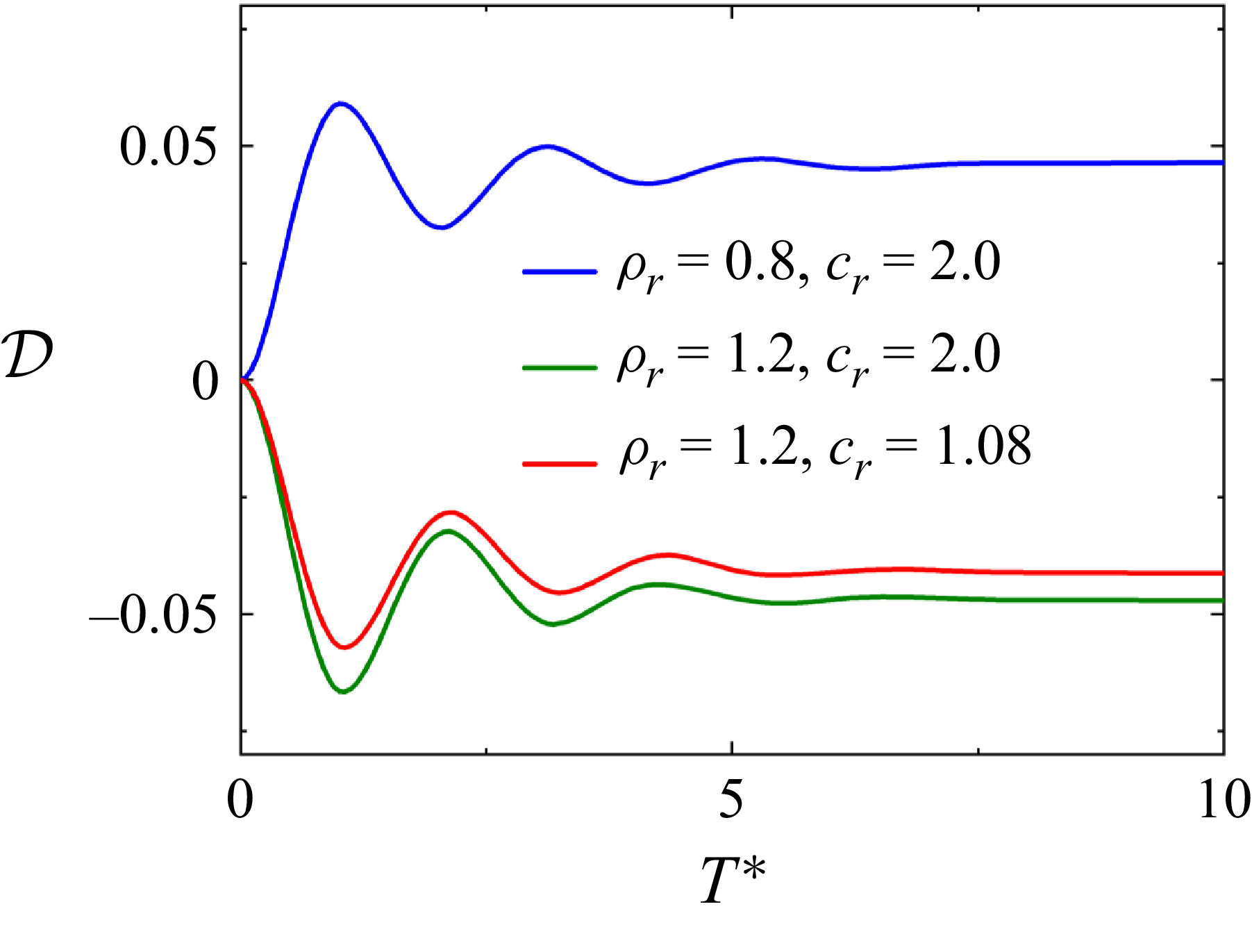


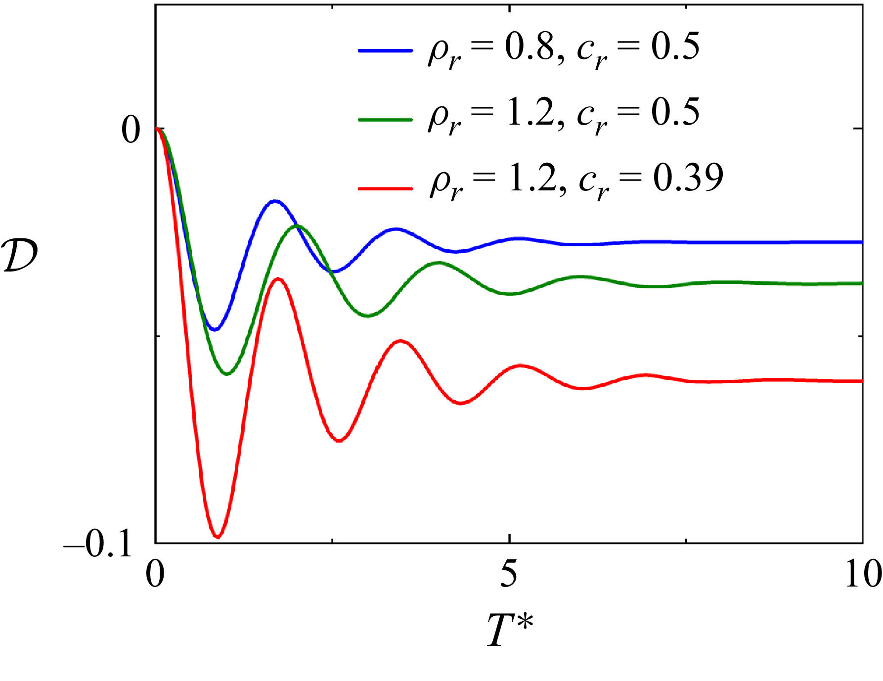


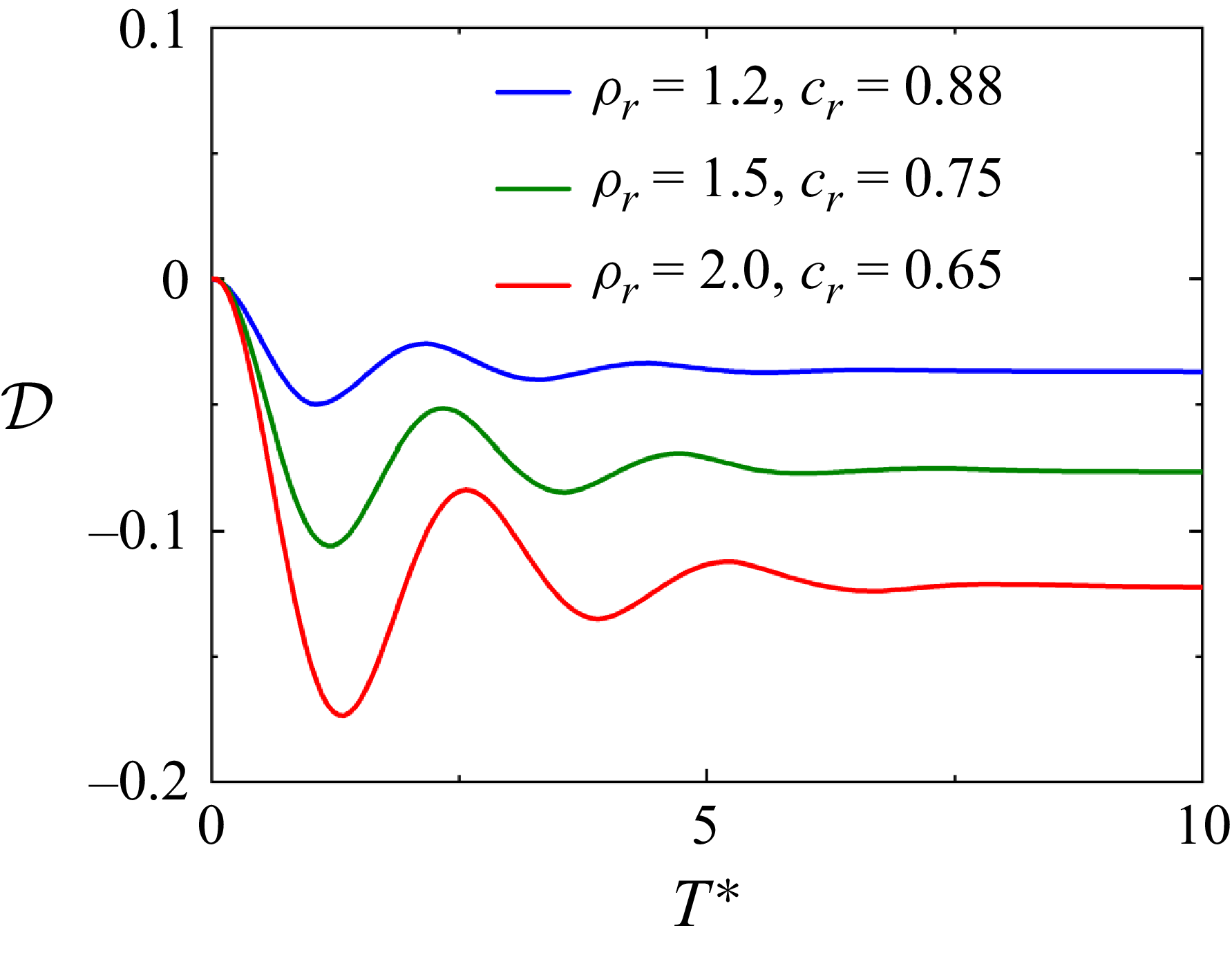


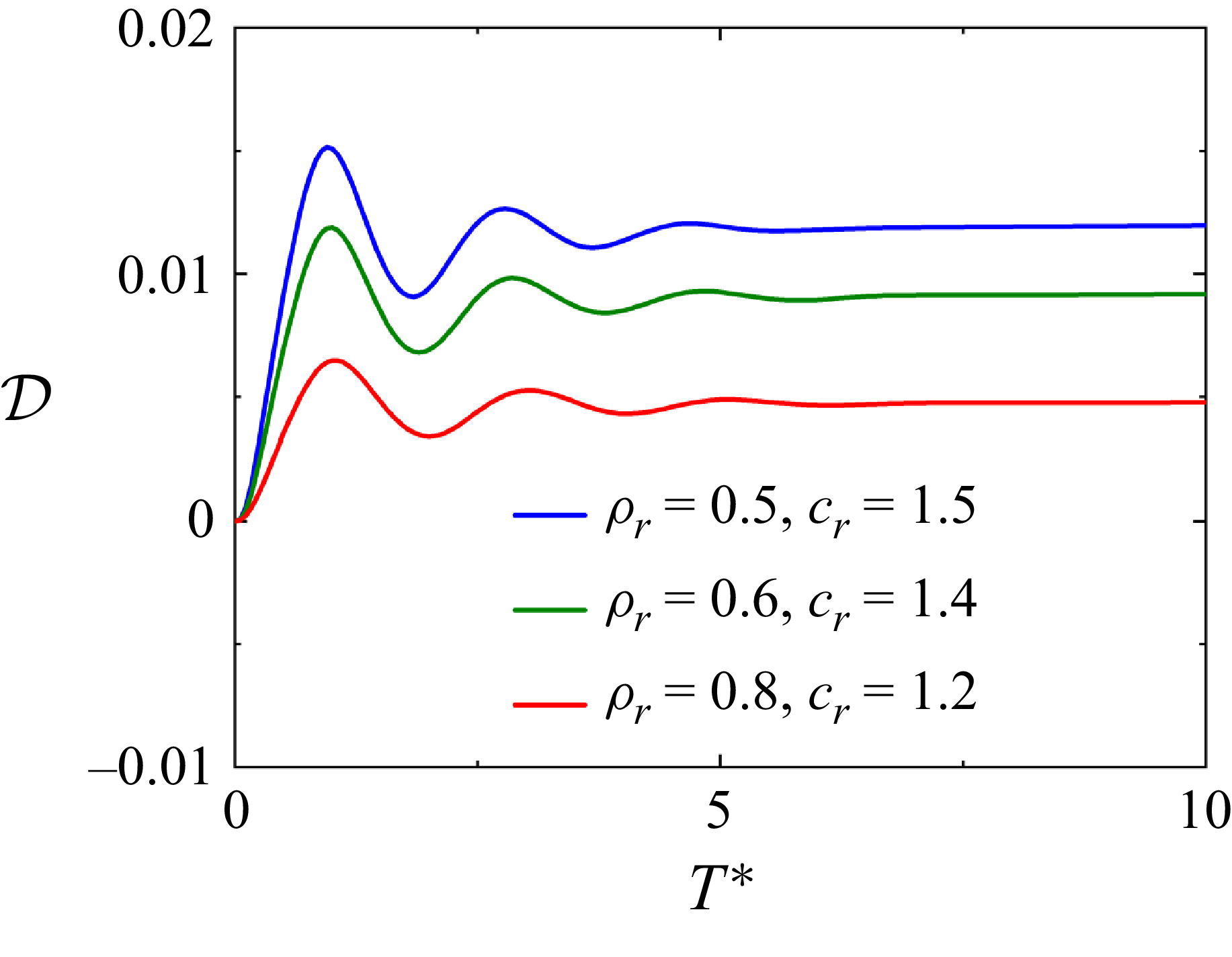


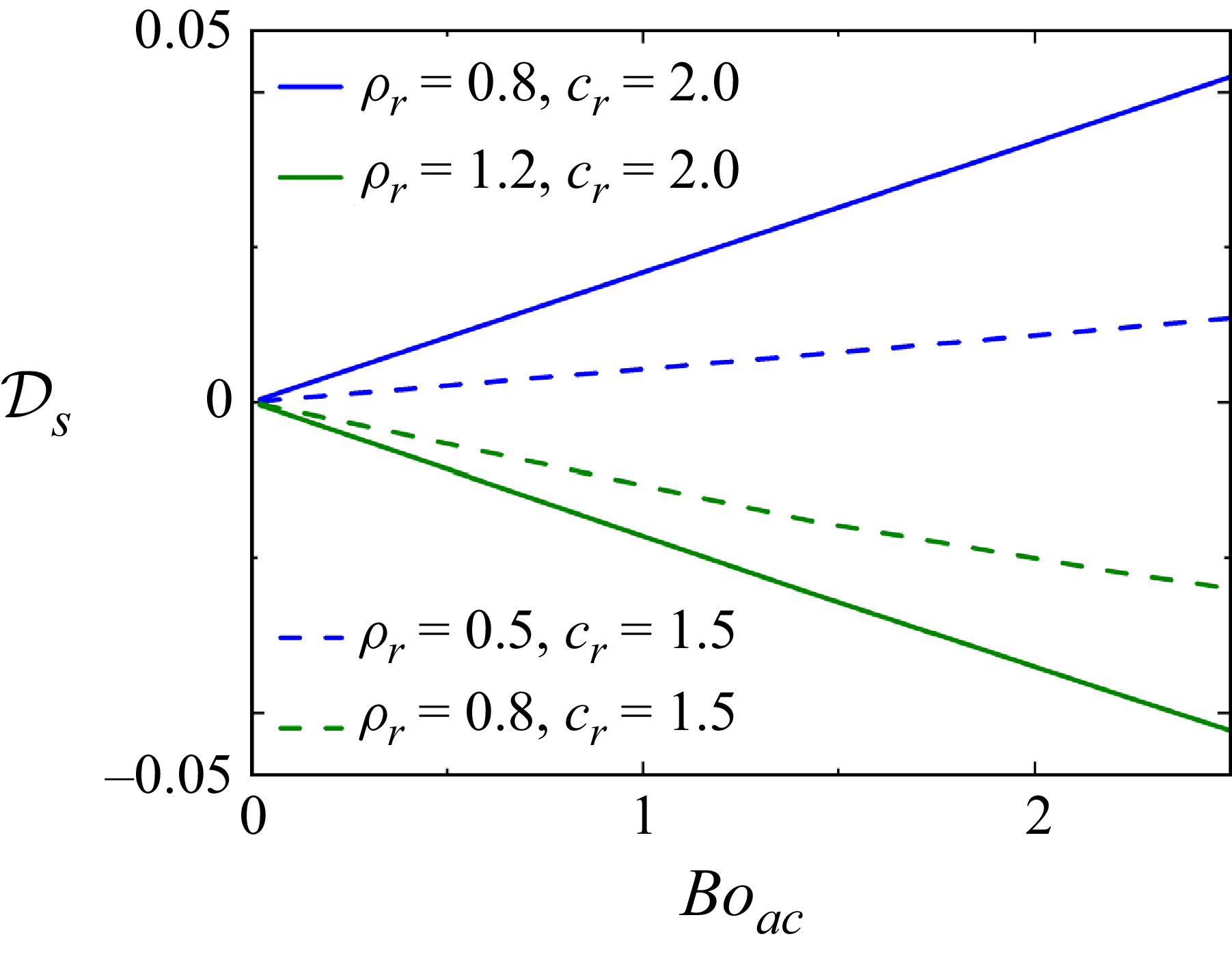


 Open access

