


1. Introduction
Stellarator optimisation traditionally used (Nührenberg et al. Reference Nührenberg, Merkel, Schwab, Schwenn, Cooper, Hayashi, Hirshman, Johnson, Monticello and Reiman1993) and still uses (Drevlak et al. Reference Drevlak, Beidler, Geiger, Helander and Turkin2018) ideal magnetohydrodynamic (MHD) proxies such as the vacuum-field magnetic well to ensure stability of the plasma equilibria. This property prevails in an ideal-MHD equilibrium if the toroidal magnetic flux, $F_{\rm T}$
, enclosed by a sequence of magnetic surfaces between the magnetic axis and plasma edge increases more strongly than the corresponding enclosed volume, i.e.
$F_{\rm T}$
, enclosed by a sequence of magnetic surfaces between the magnetic axis and plasma edge increases more strongly than the corresponding enclosed volume, i.e. $\textrm{d}^2 V/\textrm{d}{F_{\rm T}}^2\lt 0$
. Already in Bernstein et al. (Reference Bernstein, Frieman, Kruskal, Kulsrud and Chandrasekhar1958), on the energy principle of MHD stability, this quantity appears as a sufficient condition for the instability of an axisymmetric system. Deepening the vacuum-field magnetic well comes at the expense of the plasma shape, resulting in more complex magnet systems. Since, on the one hand, the stability of a fusion plasma is indispensable for good confinement and, on the other hand, economical coil design is a key ingredient for the success of future stellarator devices, the importance of the concept of a vacuum-field magnetic well is assessed in the present work.
$\textrm{d}^2 V/\textrm{d}{F_{\rm T}}^2\lt 0$
. Already in Bernstein et al. (Reference Bernstein, Frieman, Kruskal, Kulsrud and Chandrasekhar1958), on the energy principle of MHD stability, this quantity appears as a sufficient condition for the instability of an axisymmetric system. Deepening the vacuum-field magnetic well comes at the expense of the plasma shape, resulting in more complex magnet systems. Since, on the one hand, the stability of a fusion plasma is indispensable for good confinement and, on the other hand, economical coil design is a key ingredient for the success of future stellarator devices, the importance of the concept of a vacuum-field magnetic well is assessed in the present work.
The work presented here studied helical-axis stellarator configurations that lack stabilisation by a vacuum-field magnetic well. In addition, unlike other studies, a broader physical picture was chosen to highlight the differences and similarities between linear ideal-MHD and gyrokinetics (GK). It is well known that the reduced-MHD equations can be derived from gyrofluid equations (Brizard Reference Brizard1992) and, furthermore, that there is a significant correlation between reduced MHD and nonlinear GK (Brizard & Hahm Reference Brizard and Hahm2007). Moreover, in nonlinear GK, turbulent and large-scale structures regulate each other. This indicates that it is crucial to master the MHD-limit scenario as a prerequisite for high-fidelity GK turbulence simulations. Furthermore, it is still an open question if the stability limit given by ideal-MHD is decisively influenced by GK effects.
Examples of stellarator MHD stability studies have earlier been published by Ramasamy et al. (Reference Ramasamy, Aleynikova, Nikulsin, Hindenlang, Holod, Strumberger and Hoelzl2024) and Zhou et al. (Reference Zhou, Aleynikova, Liu and Ferraro2024). In the former global, nonlinear, reduced-MHD and linear-MHD calculations were done using the $\mathsf{ JOREK}$
and
$\mathsf{ JOREK}$
and $\mathsf{ CASTOR3D}$
codes in applications studying the W7-AS stellarator. The latter discusses nonlinear resistive MHD calculations done with the
$\mathsf{ CASTOR3D}$
codes in applications studying the W7-AS stellarator. The latter discusses nonlinear resistive MHD calculations done with the $\mathsf{ M3D-C1}$
code focusing on the optimised stellarator Wendelstein 7-X (W7-X).
$\mathsf{ M3D-C1}$
code focusing on the optimised stellarator Wendelstein 7-X (W7-X).
In tokamak research, many authors discuss the relationship of the fields of MHD and GK. An example is the work of Brochard et al. (Reference Brochard2022) who describe a linear verification of the GK $\mathsf{ GTC}$
code against kinetic-MHD codes in the ideal-MHD limit studying internal kink modes in the DIII-D tokamak. An equivalent study for pressure-driven modes in stellarators has not yet been provided and is therefore one of the aims of the present work.
$\mathsf{ GTC}$
code against kinetic-MHD codes in the ideal-MHD limit studying internal kink modes in the DIII-D tokamak. An equivalent study for pressure-driven modes in stellarators has not yet been provided and is therefore one of the aims of the present work.
Currently, only a few codes are able to perform the complex task of global, GK simulations in stellarator scenarios, among them $\mathsf{ GENE-3D}$
(Wilms et al. Reference Wilms, Bañón Navarro, Windisch, Bozhenkov, Warmer, Fuchert, Ford, Zhang and Stange2024),
$\mathsf{ GENE-3D}$
(Wilms et al. Reference Wilms, Bañón Navarro, Windisch, Bozhenkov, Warmer, Fuchert, Ford, Zhang and Stange2024), $\mathsf{ XGC-S}$
(Cole et al. Reference Cole, Hager, Moritaka, Dominski, Kleiber, Ku, Lazerson, Riemann and Chang2019) and
$\mathsf{ XGC-S}$
(Cole et al. Reference Cole, Hager, Moritaka, Dominski, Kleiber, Ku, Lazerson, Riemann and Chang2019) and $\mathsf{ EUTERPE}$
(Kleiber et al. Reference Kleiber2024). The latter two fall in the category of Lagrangian particle-in-cell (PIC) codes, while
$\mathsf{ EUTERPE}$
(Kleiber et al. Reference Kleiber2024). The latter two fall in the category of Lagrangian particle-in-cell (PIC) codes, while $\mathsf{ GENE-3D}$
is grid-based and uses an Eulerian description.
$\mathsf{ GENE-3D}$
is grid-based and uses an Eulerian description.
Given that low-mode-number perturbations have the potential to impact a large plasma volume, they are the subject of this study. Therefore, the simulations need to be full radius (magnetic axis to plasma boundary) and full torus (including all field periods of the configuration). The nonlinear, electromagnetic $\mathsf{ EUTERPE}$
simulations presented below combine this geometrical set-up and the usage of kinetic ions and electrons at a realistic mass ratio. To the authors’ best knowledge, it is the first time that this combination of objectives was achieved in GK simulations for a stellarator scenario.
$\mathsf{ EUTERPE}$
simulations presented below combine this geometrical set-up and the usage of kinetic ions and electrons at a realistic mass ratio. To the authors’ best knowledge, it is the first time that this combination of objectives was achieved in GK simulations for a stellarator scenario.
The paper is structured as follows. The description of the plasma equilibria is followed by brief overviews on the models and methods used in the MHD-stability and GK calculations. Details of the numerical set-up are given in § 5. In the first part of § 6, a comparison of linear-ideal-MHD stability and linear-phase nonlinear GK simulations is given, followed, in the second part, by a discussion of points specific to the GK simulations such as zonal components and the evolution of islands. Finally, a summary with conclusions and an outlook are given.
2. Description of equilibria
The Wendelstein 7-X configuration space was developed on the basis of the so-called HELIAS concept (Nührenberg & Zille Reference Nührenberg and Zille1986; Beidler et al. Reference Beidler1990). In the present work, the object of study are sequences of HELIAS configurations, i.e. helical-axis stellarators, with either the vacuum-field magnetic well or the volume-averaged plasma- $\beta$
chosen as scan parameter. (Throughout this paper,
$\beta$
chosen as scan parameter. (Throughout this paper, $\beta$
denotes the ratio of the flux-surface averages of the plasma and the magnetic pressures;
$\beta$
denotes the ratio of the flux-surface averages of the plasma and the magnetic pressures; $\langle \beta \rangle$
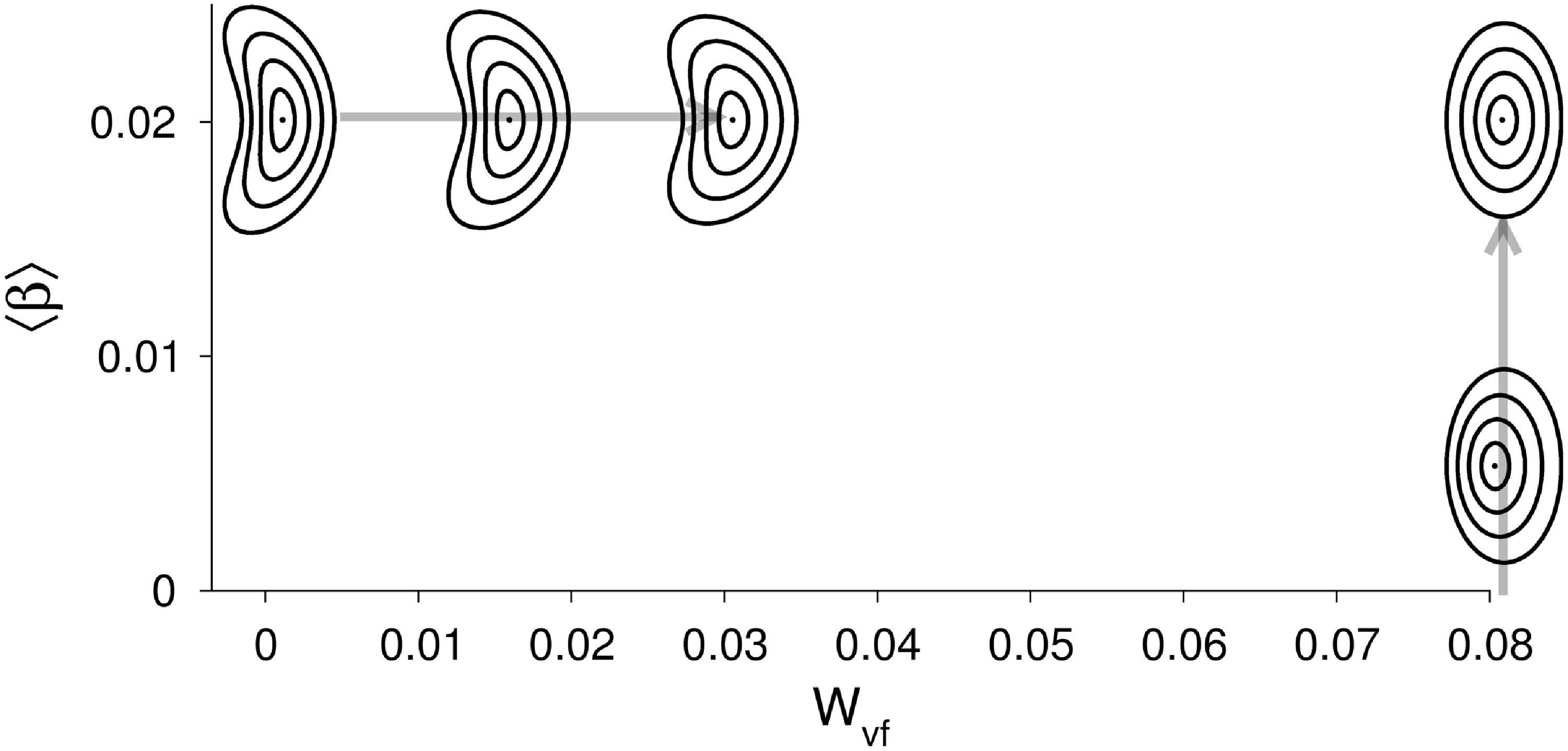
stands for the respective volume average.) Figure 1 shows the variation of the plasma cross-sections in half a field period for the simplest and for the geometrically most demanding cases, while figure 2 gives an overview of the equilibrium sequences by showing the
$\langle \beta \rangle$
stands for the respective volume average.) Figure 1 shows the variation of the plasma cross-sections in half a field period for the simplest and for the geometrically most demanding cases, while figure 2 gives an overview of the equilibrium sequences by showing the $\varphi =0^{\textrm{o}}$
cross-sections of five exemplary cases. The simplest case is a so-called
$\varphi =0^{\textrm{o}}$
cross-sections of five exemplary cases. The simplest case is a so-called $\ell =1,2$
stellarator with turning-ellipse cross-sections. It is used to study the influence of an increasing plasma pressure. Keeping the plasma pressure fixed, the second sequence of equilibria allows us to study the effect of boundary shaping and the vacuum-field magnetic well. Going to the more strongly shaped configurations, the plasma boundaries exhibit simultaneously increasing indentation, ellipticity and triangularity. The description of the plasma boundaries for all of the cases is given in Appendix A. For the
$\ell =1,2$
stellarator with turning-ellipse cross-sections. It is used to study the influence of an increasing plasma pressure. Keeping the plasma pressure fixed, the second sequence of equilibria allows us to study the effect of boundary shaping and the vacuum-field magnetic well. Going to the more strongly shaped configurations, the plasma boundaries exhibit simultaneously increasing indentation, ellipticity and triangularity. The description of the plasma boundaries for all of the cases is given in Appendix A. For the $\ell =1,2$
case, the helical excursion of the magnetic axis is roughly the size of the minor radius (denoted by
$\ell =1,2$
case, the helical excursion of the magnetic axis is roughly the size of the minor radius (denoted by $a$
) vertically and
$a$
) vertically and $1.5\, a$
horizontally. Therefore, even the
$1.5\, a$
horizontally. Therefore, even the $\ell =1,2$
case has, on the one hand, enough geometrical and, hence, magnetic-field complexity to be a meaningful object of study, but is, on the other hand, simple enough as a test bed.
$\ell =1,2$
case has, on the one hand, enough geometrical and, hence, magnetic-field complexity to be a meaningful object of study, but is, on the other hand, simple enough as a test bed.
Cross-sections of helical-axis stellarators shown at the beginning, at a quarter and at the middle of a field period. Left: turning-ellipse plasma boundary, right: HELIAS configuration with indentation and triangularity. Only five of the total of 800 magnetic surfaces are shown.
Overview of the equilibrium sequences and their dependency on the vacuum-field magnetic anti-well ( $\mathcal{W}_{{\rm vf}}$
) and the volume-averaged plasma-
$\mathcal{W}_{{\rm vf}}$
) and the volume-averaged plasma- $\beta$
. Only the
$\beta$
. Only the $\varphi =0^\circ$
cross-sections are shown for five of the in total eleven equilibria. Compare figure 1 for more cross-sections.
$\varphi =0^\circ$
cross-sections are shown for five of the in total eleven equilibria. Compare figure 1 for more cross-sections.
In the following, the normalised toroidal flux, $s$
, is used as flux label with
$s$
, is used as flux label with $s=0$
at the magnetic axis and
$s=0$
at the magnetic axis and $s=1$
at the plasma boundary. Primes denote derivatives with respect to
$s=1$
at the plasma boundary. Primes denote derivatives with respect to $s$
for functions that are constant on magnetic surfaces. With
$s$
for functions that are constant on magnetic surfaces. With $V$
the contained volume of a magnetic surface with flux label
$V$
the contained volume of a magnetic surface with flux label $s$
,
$s$
, $V''\lt 0$
prevails in an equilibrium with a magnetic well, because then the enclosed volume increases less strongly than the enclosed toroidal flux. On the other hand, a magnetic hill,
$V''\lt 0$
prevails in an equilibrium with a magnetic well, because then the enclosed volume increases less strongly than the enclosed toroidal flux. On the other hand, a magnetic hill, $V''\gt 0$
, implies that the contained volume increases faster than the flux, i.e. that the magnetic field weakens in the outer regions (Greene Reference Greene1997). The magnetic well present in a vacuum field is further deepened by the plasma pressure in the case of finite plasma-
$V''\gt 0$
, implies that the contained volume increases faster than the flux, i.e. that the magnetic field weakens in the outer regions (Greene Reference Greene1997). The magnetic well present in a vacuum field is further deepened by the plasma pressure in the case of finite plasma- $\beta$
. Therefore, the vacuum-field magnetic well is an important proxy for ideal-MHD stability (Mercier Reference Mercier1962) in low-shear, net-current-free stellarators. Obviously, the pressure profile and the equilibrium must be consistent. For the series of equilibria with fixed plasma pressure and varying relative vacuum-field magnetic-well depth
$\beta$
. Therefore, the vacuum-field magnetic well is an important proxy for ideal-MHD stability (Mercier Reference Mercier1962) in low-shear, net-current-free stellarators. Obviously, the pressure profile and the equilibrium must be consistent. For the series of equilibria with fixed plasma pressure and varying relative vacuum-field magnetic-well depth $\mathcal{W}_{{\rm vf}}$
 \begin{equation} {\mathcal{W}_{{\rm vf}}} =\frac {V'(1)-V'(0)}{V'(0)} \end{equation}
ranges from a marginal magnetic well, ${\mathcal{W}_{{\rm vf}}}=-0.002$
, to a moderate magnetic anti-well or hill,
${\mathcal{W}_{{\rm vf}}}=-0.002$
, to a moderate magnetic anti-well or hill, ${\mathcal{W}_{{\rm vf}}}=0.03$
.
${\mathcal{W}_{{\rm vf}}}=0.03$
.
The $\ell =1,2$
equilibria have a constant high vacuum-field magnetic-field anti-well (
$\ell =1,2$
equilibria have a constant high vacuum-field magnetic-field anti-well ( ${\mathcal{W}_{{\rm vf}}}=0.08$
), so are more unstable to MHD; these are used for a stability scan in plasma-
${\mathcal{W}_{{\rm vf}}}=0.08$
), so are more unstable to MHD; these are used for a stability scan in plasma- $\beta$
. In stellarators the variation of the magnetic-field strength on the magnetic axis (with the minimum
$\beta$
. In stellarators the variation of the magnetic-field strength on the magnetic axis (with the minimum $B_{\rm min}$
and the maximum
$B_{\rm min}$
and the maximum $B_{\rm max}$
, here given as a relative mirror ratio)
$B_{\rm max}$
, here given as a relative mirror ratio)
 \begin{equation} {\mathcal{M}_{{\rm B}}} = \frac {B_{\mathrm{max}}-B_{\mathrm{min}}}{2\,B_{\mathrm{av}}}, \end{equation}
may be more or less pronounced; in ideal axisymmetric tokamaks it is zero. The strength of the magnetic mirror is also seen in the respective Fourier component of the magnetic-field strength, e.g. $B_{01}$
in the right panel of figure 3. For the HELIAS cases, the magnetic mirror ratio increases with increasing vacuum-field magnetic hill from
$B_{01}$
in the right panel of figure 3. For the HELIAS cases, the magnetic mirror ratio increases with increasing vacuum-field magnetic hill from ${\mathcal{M}_{{\rm B}}}=0.014$
to
${\mathcal{M}_{{\rm B}}}=0.014$
to $\approx 0.07$
. To put these numbers into context, it is useful to recall that, as a consequence of the optimisation, nearly all W7-X configurations have a vacuum-field magnetic well, e.g.
$\approx 0.07$
. To put these numbers into context, it is useful to recall that, as a consequence of the optimisation, nearly all W7-X configurations have a vacuum-field magnetic well, e.g. $\mathcal{W}_{{\rm vf}} \approx -0.01$
for the W7-X standard case, which has a mirror ratio of
$\mathcal{W}_{{\rm vf}} \approx -0.01$
for the W7-X standard case, which has a mirror ratio of ${\mathcal{M}_{{\rm B}}}\approx 0.05$
(Dinklage et al. Reference Dinklage2018). An exception is the low-
${\mathcal{M}_{{\rm B}}}\approx 0.05$
(Dinklage et al. Reference Dinklage2018). An exception is the low- $\iota$
very-high-mirror W7-X with
$\iota$
very-high-mirror W7-X with ${\mathcal{W}_{{\rm vf}}}\approx 0.0044$
and
${\mathcal{W}_{{\rm vf}}}\approx 0.0044$
and ${\mathcal{M}_{{\rm B}}}\approx 0.25$
.
${\mathcal{M}_{{\rm B}}}\approx 0.25$
.
Without much loss of generality, the so-called stellarator symmetry (Dewar & Hudson Reference Dewar and Hudson1998) is employed, which is analogous to the consideration of an up-down symmetric tokamak. Furthermore, the plasma domain is chosen to have a fourfold discrete symmetry, i.e. to consist of four identical field periods, $N_{{\rm p}}=4$
. Further equilibrium parameters are the major and minor radii of
$N_{{\rm p}}=4$
. Further equilibrium parameters are the major and minor radii of $R_0=8\,\textrm{m}$
and of
$R_0=8\,\textrm{m}$
and of $a=1\,\textrm{m}$
, and, hence, an aspect ratio of
$a=1\,\textrm{m}$
, and, hence, an aspect ratio of $A=R_0/a=8$
. The equilibria are calculated using the
$A=R_0/a=8$
. The equilibria are calculated using the $\mathsf{ VMEC}$
code (Hirshman et al. Reference Hirshman, van RIJ and Merkel1986), which relies on the assumption of nested flux surfaces and determines a general-geometry ideal-MHD equilibrium by minimisation of the total energy of the static plasma. All the equilibria studied in this work were calculated with
$\mathsf{ VMEC}$
code (Hirshman et al. Reference Hirshman, van RIJ and Merkel1986), which relies on the assumption of nested flux surfaces and determines a general-geometry ideal-MHD equilibrium by minimisation of the total energy of the static plasma. All the equilibria studied in this work were calculated with $800$
flux surfaces. In this way sufficient resolution is supplied, especially near the magnetic axis, which otherwise is poorly resolved because
$800$
flux surfaces. In this way sufficient resolution is supplied, especially near the magnetic axis, which otherwise is poorly resolved because $\mathsf{ VMEC}$
uses the normalised toroidal flux as the radial coordinate. A vanishing net toroidal current is prescribed for the equilibrium calculations, as is characteristic of stellarators without a boot-strap current. This, in turn, determines the magnetic-field-line twist or rotational transform,
$\mathsf{ VMEC}$
uses the normalised toroidal flux as the radial coordinate. A vanishing net toroidal current is prescribed for the equilibrium calculations, as is characteristic of stellarators without a boot-strap current. This, in turn, determines the magnetic-field-line twist or rotational transform, $\iota$
. Fixed-boundary equilibria are used, so that the total enclosed toroidal flux determines the magnetic-field strength. The stellarator nature of the equilibrium is also obvious from the dominant Fourier harmonics of the magnetic-field strength
$\iota$
. Fixed-boundary equilibria are used, so that the total enclosed toroidal flux determines the magnetic-field strength. The stellarator nature of the equilibrium is also obvious from the dominant Fourier harmonics of the magnetic-field strength $B$
, shown by way of example for the
$B$
, shown by way of example for the $\ell =1,2$
case in the right panel of figure 3. The surface-average
$\ell =1,2$
case in the right panel of figure 3. The surface-average $B_{0,0}$
, shown with its value on axis subtracted, is approximately unity with a variation of
$B_{0,0}$
, shown with its value on axis subtracted, is approximately unity with a variation of $\approx \pm\, 0.003$
for
$\approx \pm\, 0.003$
for $\langle \beta \rangle =0.006$
. For this case, the main helical component is stronger than the term describing the axisymmetric toroidicity, and the magnetic mirror field stronger than the tokamak ellipticity term.
$\langle \beta \rangle =0.006$
. For this case, the main helical component is stronger than the term describing the axisymmetric toroidicity, and the magnetic mirror field stronger than the tokamak ellipticity term.
Left: equilibrium profiles versus normalised effective minor radius, $r/a$
, for the
$r/a$
, for the $\ell =1,2$
case (left panel of figure 1): temperatures, densities (black dashed), pressure (black solid), all normalised to their axis value; rotational-transform profiles for
$\ell =1,2$
case (left panel of figure 1): temperatures, densities (black dashed), pressure (black solid), all normalised to their axis value; rotational-transform profiles for $0.003 \leqslant \langle \beta \rangle \leqslant 0.021$
(red to blue, right-side axis). Right: Fourier spectrum of
$0.003 \leqslant \langle \beta \rangle \leqslant 0.021$
(red to blue, right-side axis). Right: Fourier spectrum of $B$
in magnetic coordinates versus
$B$
in magnetic coordinates versus $r/a$
. Only the dominant harmonics are shown, they are:
$r/a$
. Only the dominant harmonics are shown, they are: $(m,n)=(0,0)$
(dashed black, with its value on axis subtracted),
$(m,n)=(0,0)$
(dashed black, with its value on axis subtracted), $(1,-1)$
(main helical term, black),
$(1,-1)$
(main helical term, black), $(1,0)$
(axisymmetric torus term, red),
$(1,0)$
(axisymmetric torus term, red), $(2,-1)$
(orange),
$(2,-1)$
(orange), $(0,1)$
(mirror field, blue) and
$(0,1)$
(mirror field, blue) and $(2,0)$
(axisymmetric ellipticity, cyan).
$(2,0)$
(axisymmetric ellipticity, cyan).
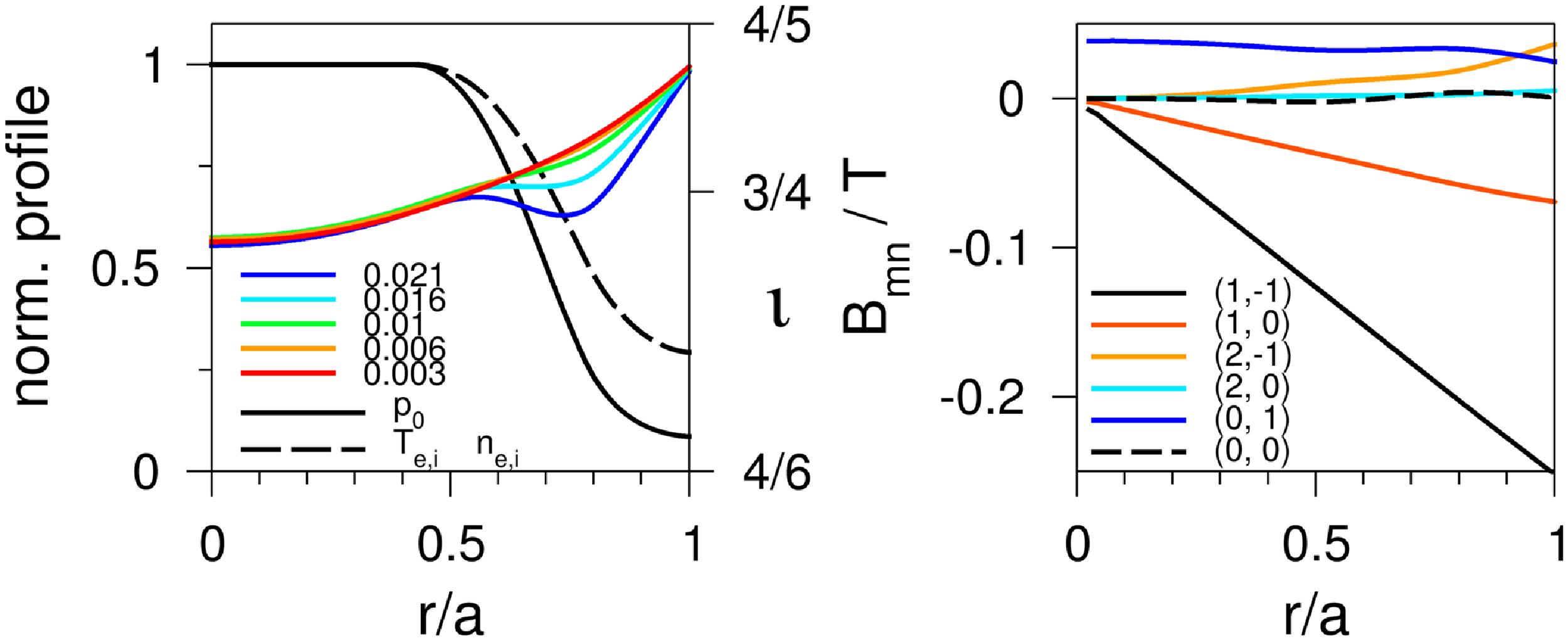
Finite-pressure equilibria are obtained with the normalised pressure profile shown in the left panel of figure 3. Identical profiles are used for the normalised ion and electron temperature $(T)$
and normalised density
$(T)$
and normalised density $(n)$
profiles (defining the normalised equilibrium pressure
$(n)$
profiles (defining the normalised equilibrium pressure $p_0$
)
$p_0$
)
 \begin{equation} T_{{\rm i,e}}/T_{{\rm i,e, \mathrm{axis}}}=n_{{\rm i,e}}/n_{{\rm i,e, \mathrm{axis}}}=\sqrt {p_0/p_{0,{ \mathrm{axis}}}}. \end{equation}
Furthermore, $T_{{{\rm i}, \mathrm{axis}}}=T_{{{\rm e}, \mathrm{axis}}}$
is chosen, and it is
$T_{{{\rm i}, \mathrm{axis}}}=T_{{{\rm e}, \mathrm{axis}}}$
is chosen, and it is $n_{{{\rm i}, \mathrm{axis}}}=n_{{{\rm e}, \mathrm{axis}}}$
in consequence of the assumed quasi-neutrality. With this setting the ratio of the logarithmic derivatives is unity for all species, i.e.
$n_{{{\rm i}, \mathrm{axis}}}=n_{{{\rm e}, \mathrm{axis}}}$
in consequence of the assumed quasi-neutrality. With this setting the ratio of the logarithmic derivatives is unity for all species, i.e.
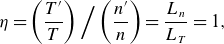 \begin{equation} \eta = \left ( \frac {T'}{T} \right ) \Big / \left ( \frac {n'}{n} \right ) = \frac {L_n}{L_T} =1, \end{equation}
with $L_n$
and
$L_n$
and $L_T$
the normalised gradient scale lengths of unperturbed density and temperature. In § 6, additionally, an equilibrium is studied with identical pressure profile, but composed of a steeper temperature and a flat-density profile. The normalised profiles,
$L_T$
the normalised gradient scale lengths of unperturbed density and temperature. In § 6, additionally, an equilibrium is studied with identical pressure profile, but composed of a steeper temperature and a flat-density profile. The normalised profiles, $f(s)$
, are defined by a hat function,
$f(s)$
, are defined by a hat function, $g(s)$
, viz.
$g(s)$
, viz.
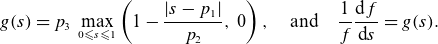 \begin{equation} g(s)=p_3\,\max _{0\leqslant s\leqslant 1}\left (1-\frac {|s - p_1|}{p_2}, \; 0\right ) , \quad \textrm{and} \quad \frac {1}{f} \frac {\textrm{d} f}{\textrm{d} s}=g(s). \end{equation}
For the dashed profile in the left panel of figure 3, the parameters are $p_1=0.6$
, which is the location of the maximum gradient,
$p_1=0.6$
, which is the location of the maximum gradient, $p_2=0.85$
, the width of the gradient region,
$p_2=0.85$
, the width of the gradient region, $p_3=-2.9$
, the maximum of the logarithmic derivative, and
$p_3=-2.9$
, the maximum of the logarithmic derivative, and $f(0)=1$
for the normalisation. The normalised pressure is
$f(0)=1$
for the normalisation. The normalised pressure is $f^2$
, shown by the solid, black line in the left panel of figure 3. A sequence of equilibria with the volume-averaged plasma-
$f^2$
, shown by the solid, black line in the left panel of figure 3. A sequence of equilibria with the volume-averaged plasma- $\beta$
as scan parameter is established by a factor of
$\beta$
as scan parameter is established by a factor of $\sqrt {\langle \beta \rangle /0.021}$
for the densities and temperatures and a factor of
$\sqrt {\langle \beta \rangle /0.021}$
for the densities and temperatures and a factor of $\langle \beta \rangle$
for the pressure applied to the on-axis values given in table 2, with
$\langle \beta \rangle$
for the pressure applied to the on-axis values given in table 2, with $\langle \beta \rangle$
the needed value of the volume-averaged plasma-
$\langle \beta \rangle$
the needed value of the volume-averaged plasma- $\beta$
. Without a plasma pressure, the rotational transform varies as
$\beta$
. Without a plasma pressure, the rotational transform varies as $4/6 \lt 0.73 \lesssim \iota \lesssim 0.79 \lt 4/5$
in all equilibria, thus avoiding the low-order natural resonances of four-period stellarators which are in general connected to magnetic islands (Grad Reference Grad1967; Boozer Reference Boozer1984; Waelbroeck Reference Waelbroeck2009). Depending on the local steepness of the pressure profile the rotational transform locally decreases in the region of the pressure gradient (Freidberg Reference Freidberg2014). Using the
$4/6 \lt 0.73 \lesssim \iota \lesssim 0.79 \lt 4/5$
in all equilibria, thus avoiding the low-order natural resonances of four-period stellarators which are in general connected to magnetic islands (Grad Reference Grad1967; Boozer Reference Boozer1984; Waelbroeck Reference Waelbroeck2009). Depending on the local steepness of the pressure profile the rotational transform locally decreases in the region of the pressure gradient (Freidberg Reference Freidberg2014). Using the $\ell =1,2$
case as an example, the dependence of
$\ell =1,2$
case as an example, the dependence of $\iota$
on the plasma-
$\iota$
on the plasma- $\beta$
is also shown in the left panel of figure 3.
$\beta$
is also shown in the left panel of figure 3.
The Alfvén time is often used to normalise growth rates. Defining it with the minor radius $a$
and the average field strength at the magnetic axis
$a$
and the average field strength at the magnetic axis $B_0$
as
$B_0$
as
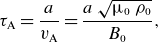 \begin{equation} \tau_{\mathrm{A}}= \frac {a}{v_{{\rm A}}}= \frac {a\,\sqrt {\unicode{x03BC} _0\,\rho _0}}{B_0}, \end{equation}
a value of $\approx 0.27\,\unicode{x03BC} \textrm{s}$
is obtained for the
$\approx 0.27\,\unicode{x03BC} \textrm{s}$
is obtained for the $\ell =1,2$
and the HELIAS cases, all equilibria at
$\ell =1,2$
and the HELIAS cases, all equilibria at $\langle \beta \rangle =0.021$
.
$\langle \beta \rangle =0.021$
.
3. Magnetohydrodynamic stability
In the following sections, perturbed quantities are indicated by a $\delta$
, e.g. the perturbed magnetic field,
$\delta$
, e.g. the perturbed magnetic field, $\delta \boldsymbol{B}$
, whereas
$\delta \boldsymbol{B}$
, whereas $\boldsymbol{B}$
stands for the unperturbed field. In the model of linearised ideal MHD, the time evolution of the Lagrangian displacement vector,
$\boldsymbol{B}$
stands for the unperturbed field. In the model of linearised ideal MHD, the time evolution of the Lagrangian displacement vector, $\boldsymbol \xi$
, describes the perturbation of the equilibrium state. The linearisation of, e.g. the ideal induction equation, determines the perturbed magnetic field
$\boldsymbol \xi$
, describes the perturbation of the equilibrium state. The linearisation of, e.g. the ideal induction equation, determines the perturbed magnetic field
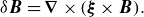 \begin{equation} \delta \boldsymbol{B} = {\boldsymbol \nabla \,\times\,} (\boldsymbol \xi {\,\times\,} \boldsymbol{B}). \end{equation}
The work of Bernstein et al. (Reference Bernstein, Frieman, Kruskal, Kulsrud and Chandrasekhar1958) and Hain et al. (Reference Hain, Lüst and Schlüter1957), in which the time evolution of $\boldsymbol \xi$
is formulated in weak form
$\boldsymbol \xi$
is formulated in weak form
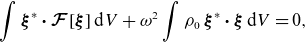 \begin{equation} \int \boldsymbol \xi ^\ast \boldsymbol{\cdot} {\mathcal F}\,\lbrack \boldsymbol{\xi} \rbrack \,\textrm{d} V + \omega ^2 \int \rho _0\, \boldsymbol{\xi}^{\ast} \boldsymbol{\cdot} \boldsymbol{\xi} \,\textrm{d} V =0, \end{equation}
laid the basis of the field. In equation (3.2), the volume integrals extend over the plasma and, potentially, over a surrounding vacuum domain. The equilibrium mass density is $\rho _0$
. An asterisk superscript stands for the complex conjugate. The ideal-MHD force operator
$\rho _0$
. An asterisk superscript stands for the complex conjugate. The ideal-MHD force operator $\mathcal{F}$
has time-independent coefficients, therefore allowing the separation of time and space dependences. Furthermore, it is Hermitian and is bounded from below. Correa-Restrepo (Reference Correa-Restrepo1978), e.g. gives an intuitive, coordinate-free formulation of the first term of equation (3.2). For ease of reading, it is repeated in Appendix B. The Hermiticity of the force operator is obvious in this representation, equation (B.1). Field-line bending and the two compression terms, namely field and fluid compression, stabilise perturbations, while the combination of equilibrium pressure gradient and curvature and the equilibrium parallel-current density are the source of pressure and current-driven instabilities.
$\mathcal{F}$
has time-independent coefficients, therefore allowing the separation of time and space dependences. Furthermore, it is Hermitian and is bounded from below. Correa-Restrepo (Reference Correa-Restrepo1978), e.g. gives an intuitive, coordinate-free formulation of the first term of equation (3.2). For ease of reading, it is repeated in Appendix B. The Hermiticity of the force operator is obvious in this representation, equation (B.1). Field-line bending and the two compression terms, namely field and fluid compression, stabilise perturbations, while the combination of equilibrium pressure gradient and curvature and the equilibrium parallel-current density are the source of pressure and current-driven instabilities.
The two MHD codes used in the present study are $\mathsf{ CAS3D}$
(Schwab Reference Schwab1993) and
$\mathsf{ CAS3D}$
(Schwab Reference Schwab1993) and $\mathsf{ CKA}$
(Slaby et al. Reference Slaby, Könies and Kleiber2024). While the former is based on (3.2) and uses the full formalism of linearised ideal MHD, the
$\mathsf{ CKA}$
(Slaby et al. Reference Slaby, Könies and Kleiber2024). While the former is based on (3.2) and uses the full formalism of linearised ideal MHD, the $\mathsf{ CKA}$
code employs the picture of reduced MHD.
$\mathsf{ CKA}$
code employs the picture of reduced MHD.
4. Gyrokinetic model
In this work, the $\mathsf{ EUTERPE}$
code is used to perform spatially global, nonlinear, electromagnetic, GK simulations with electrons and ions as kinetic species at physical mass ratio. Collision operators are available in
$\mathsf{ EUTERPE}$
code is used to perform spatially global, nonlinear, electromagnetic, GK simulations with electrons and ions as kinetic species at physical mass ratio. Collision operators are available in $\mathsf{ EUTERPE}$
, but are not included in the present study. An in-depth description of the GK model used and of the code itself are given in Kleiber et al. (Reference Kleiber2024), of which only a few basics are summarised here and in Appendices C, D and E. Problems inherent to PIC techniques are addressed by means of the
$\mathsf{ EUTERPE}$
, but are not included in the present study. An in-depth description of the GK model used and of the code itself are given in Kleiber et al. (Reference Kleiber2024), of which only a few basics are summarised here and in Appendices C, D and E. Problems inherent to PIC techniques are addressed by means of the $\delta{f}$
-ansatz (i.e. the distribution function
$\delta{f}$
-ansatz (i.e. the distribution function $f$
is split into a time-independent part
$f$
is split into a time-independent part $f_0$
and a time-dependent part
$f_0$
and a time-dependent part $\delta{f}$
) and a pull-back transformation for the mitigation of the cancellation problem (Mishchenko et al. Reference Mishchenko, Könies, Kleiber and Cole2014, Reference Mishchenko, Biancalani, Bottino, Hayward-Schneider, Lauber, Lanti, Villard, Kleiber, Könies and Borchardt2021). For the ions/electrons,
$\delta{f}$
) and a pull-back transformation for the mitigation of the cancellation problem (Mishchenko et al. Reference Mishchenko, Könies, Kleiber and Cole2014, Reference Mishchenko, Biancalani, Bottino, Hayward-Schneider, Lauber, Lanti, Villard, Kleiber, Könies and Borchardt2021). For the ions/electrons, $f_0$
is chosen as an unshifted/shifted Maxwellian distribution, so that a potentially existing equilibrium current is carried by the electrons only. For ease of reference, the equations of motion of the PIC marker particles are included in Appendix C, the field equations for the perturbation quantities
$f_0$
is chosen as an unshifted/shifted Maxwellian distribution, so that a potentially existing equilibrium current is carried by the electrons only. For ease of reference, the equations of motion of the PIC marker particles are included in Appendix C, the field equations for the perturbation quantities $\delta \Phi$
,
$\delta \Phi$
, $\delta A_{\|}$
and
$\delta A_{\|}$
and $\delta B_{\|}$
are summarised in Appendix D. The
$\delta B_{\|}$
are summarised in Appendix D. The $\mathsf{ EUTERPE}$
code implements a splitting technique for the scalar perturbed parallel vector potential,
$\mathsf{ EUTERPE}$
code implements a splitting technique for the scalar perturbed parallel vector potential, $\delta A_{\|}$
, employing a symplectic and a Hamiltonian part, see equation (C.1). The perturbed magnetic field is defined as
$\delta A_{\|}$
, employing a symplectic and a Hamiltonian part, see equation (C.1). The perturbed magnetic field is defined as
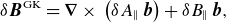 \begin{equation} \delta \boldsymbol{B}^{{\rm GK}} = {\boldsymbol \nabla \,\times\,} \left ( \delta A_{\|}\,\boldsymbol{b}\right ) + \delta B_{\|}\, \boldsymbol{b}, \end{equation}
i.e. using $\boldsymbol{b}\boldsymbol \cdot {\boldsymbol \nabla \,\times\,}\delta {\boldsymbol{A}}_\perp \approx \delta B_{\|}$
. Dong et al. (Reference Dong, Bao, Bhattacharjee, Brizard, Lin and Porazik2017), for example, describe the inclusion of the
$\boldsymbol{b}\boldsymbol \cdot {\boldsymbol \nabla \,\times\,}\delta {\boldsymbol{A}}_\perp \approx \delta B_{\|}$
. Dong et al. (Reference Dong, Bao, Bhattacharjee, Brizard, Lin and Porazik2017), for example, describe the inclusion of the $\delta B_{\|}$
term in the
$\delta B_{\|}$
term in the $\mathsf{ GTC}$
code and its importance for internal current-driven perturbation in DIII-D scenarios. Joiner et al. (Reference Joiner, Hirose and Dorland2010) discuss the role of the compressional
$\mathsf{ GTC}$
code and its importance for internal current-driven perturbation in DIII-D scenarios. Joiner et al. (Reference Joiner, Hirose and Dorland2010) discuss the role of the compressional $\delta B_{\|}$
for various micro-turbulence modes employing results from the flux-tube-based GK code
$\delta B_{\|}$
for various micro-turbulence modes employing results from the flux-tube-based GK code $\mathsf{ GS2}$
. In local linear micro-stability calculations for the spherical-tokamak fusion power plant (Kennedy et al. 2023), inclusion of
$\mathsf{ GS2}$
. In local linear micro-stability calculations for the spherical-tokamak fusion power plant (Kennedy et al. 2023), inclusion of $\delta B_{\|}$
proved essential for instability of the dominant hybrid-kinetic-ballooning modes. This is now understood to be due to strong stabilisation by
$\delta B_{\|}$
proved essential for instability of the dominant hybrid-kinetic-ballooning modes. This is now understood to be due to strong stabilisation by $\textrm{d}\beta /\textrm{d}\rho$
, taking the equilibrium close to marginal stability (Kennedy et al. Reference Kennedy2024). Consequently, the latter work found that including
$\textrm{d}\beta /\textrm{d}\rho$
, taking the equilibrium close to marginal stability (Kennedy et al. Reference Kennedy2024). Consequently, the latter work found that including $\delta B_{\|}$
is not required for local instability in tokamak equilibria at lower values of
$\delta B_{\|}$
is not required for local instability in tokamak equilibria at lower values of $\textrm{d}\beta /\textrm{d}\rho$
. In an analysis that adopts a ballooning-space approximation, Zocco et al. (Reference Zocco, Helander and Connor2015) highlight the significance of
$\textrm{d}\beta /\textrm{d}\rho$
. In an analysis that adopts a ballooning-space approximation, Zocco et al. (Reference Zocco, Helander and Connor2015) highlight the significance of $\delta B_{\|}$
for the stability of ion-temperature-gradient-driven modes. The role of the
$\delta B_{\|}$
for the stability of ion-temperature-gradient-driven modes. The role of the $\delta B_{\|}$
term for the scenario studied here is discussed in § 6.1.
$\delta B_{\|}$
term for the scenario studied here is discussed in § 6.1.
For the comparison of ideal-MHD and GK results, equations are derived connecting the displacement $\boldsymbol \xi$
, more specifically its component normal to flux surfaces, and the perturbed potentials
$\boldsymbol \xi$
, more specifically its component normal to flux surfaces, and the perturbed potentials $\delta \Phi$
and
$\delta \Phi$
and $\delta A_{\|}$
through their directional derivatives along the unperturbed field-line orthogonals. In the following,
$\delta A_{\|}$
through their directional derivatives along the unperturbed field-line orthogonals. In the following, $\delta \boldsymbol{A} = \delta A_{\|}\boldsymbol{b}$
is adopted for the perturbed vector potential as it is done in the reduced-MHD model and, often, in the GK approach. Furthermore, a purely exponential growth in time with growth rate
$\delta \boldsymbol{A} = \delta A_{\|}\boldsymbol{b}$
is adopted for the perturbed vector potential as it is done in the reduced-MHD model and, often, in the GK approach. Furthermore, a purely exponential growth in time with growth rate $\gamma$
,
$\gamma$
, $\propto \exp {(\gamma \,t)}$
, is assumed. Then, from the ideal Ohm’s law,
$\propto \exp {(\gamma \,t)}$
, is assumed. Then, from the ideal Ohm’s law, $\boldsymbol{E} + \boldsymbol{v} {\,\times\,} \boldsymbol{B} = 0$
, and the representation of the perturbed electric field,
$\boldsymbol{E} + \boldsymbol{v} {\,\times\,} \boldsymbol{B} = 0$
, and the representation of the perturbed electric field,
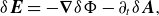 \begin{equation} \delta \boldsymbol{E} = -{\boldsymbol \nabla }\delta \Phi - \partial _t \delta \boldsymbol{A}, \end{equation}
an equation for the perturbed electrostatic potential, $\delta \Phi$
, is obtained
$\delta \Phi$
, is obtained
 \begin{equation} {\boldsymbol \nabla } s {\,\times\,} \boldsymbol{B} \boldsymbol \cdot {\boldsymbol \nabla }\delta \Phi = \gamma \, B^2\, \boldsymbol \xi \boldsymbol \cdot {\boldsymbol \nabla } s, \end{equation}
with ${\boldsymbol \nabla } s/|{\boldsymbol \nabla } s|$
the outer unit normal of an equilibrium flux surface. Analogously, the equation for the scalar perturbed vector potential,
${\boldsymbol \nabla } s/|{\boldsymbol \nabla } s|$
the outer unit normal of an equilibrium flux surface. Analogously, the equation for the scalar perturbed vector potential, $\delta A_{\|}$
, reads as
$\delta A_{\|}$
, reads as
 \begin{equation} {\boldsymbol \nabla } s {\,\times\,} \boldsymbol{B} \boldsymbol \cdot {\boldsymbol \nabla } \left ( \frac {\delta A_{\|}}{B} \right ) = - \boldsymbol{B} \boldsymbol \cdot {\boldsymbol \nabla } ( \boldsymbol \xi \boldsymbol \cdot {\boldsymbol \nabla } s ). \end{equation}
This relation is obtained by dotting $\delta \boldsymbol{B}^{\rm{MHD}} ={\boldsymbol \nabla \,\times\,} (\boldsymbol \xi {\,\times\,} \boldsymbol{B})$
and
$\delta \boldsymbol{B}^{\rm{MHD}} ={\boldsymbol \nabla \,\times\,} (\boldsymbol \xi {\,\times\,} \boldsymbol{B})$
and $\delta \boldsymbol{B}^{\rm{GK}} ={\boldsymbol \nabla \,\times\,} (\delta A_{\|} \boldsymbol{b})$
with
$\delta \boldsymbol{B}^{\rm{GK}} ={\boldsymbol \nabla \,\times\,} (\delta A_{\|} \boldsymbol{b})$
with ${\boldsymbol \nabla } s$
. Anticipating the results shown in figure 6, the component parallel to the background magnetic field is neglected in the GK perturbed magnetic field. Equation (4.4) is then derived using vector calculus and the fact that
${\boldsymbol \nabla } s$
. Anticipating the results shown in figure 6, the component parallel to the background magnetic field is neglected in the GK perturbed magnetic field. Equation (4.4) is then derived using vector calculus and the fact that ${\boldsymbol \nabla } s$
is normal to the equilibrium magnetic field and the equilibrium current density.
${\boldsymbol \nabla } s$
is normal to the equilibrium magnetic field and the equilibrium current density.
5. Numerical set-up
An inspection of the ideal-MHD energy functional, equation (B.1), shows that the stabilising contributions are minimised by perturbations fulfilling the resonance condition $k_{\|}\approx 0$
or
$k_{\|}\approx 0$
or $m\,\iota + n \approx 0$
, with
$m\,\iota + n \approx 0$
, with $m$
and
$m$
and $n$
the poloidal and toroidal perturbation mode numbers. For the equilibria described in § 2 and figure 3, the low-order rational
$n$
the poloidal and toroidal perturbation mode numbers. For the equilibria described in § 2 and figure 3, the low-order rational $\iota =3/4$
is located at approximately mid-radius. Hence, perturbations that are dominated by harmonics
$\iota =3/4$
is located at approximately mid-radius. Hence, perturbations that are dominated by harmonics $(m,n)=k(4,-3)$
, with integer
$(m,n)=k(4,-3)$
, with integer $k$
, are near resonant. Owing to the small shear of the rotational transform (left panel of figure 3), side bands of the dominant harmonic are resonant only for large multiples
$k$
, are near resonant. Owing to the small shear of the rotational transform (left panel of figure 3), side bands of the dominant harmonic are resonant only for large multiples $k$
. For example, tokamak-type side bands with
$k$
. For example, tokamak-type side bands with $(m,n)=(4 k\pm 1, -3 k)$
are resonant only for
$(m,n)=(4 k\pm 1, -3 k)$
are resonant only for $k\gtrsim 5$
, given the variation of the rotational transform,
$k\gtrsim 5$
, given the variation of the rotational transform, $0.7\lt \iota \lt 0.8$
. This is different for stellarator-type couplings, which lead to resonant side bands even for
$0.7\lt \iota \lt 0.8$
. This is different for stellarator-type couplings, which lead to resonant side bands even for $k=1$
. Examples are the resonant harmonics
$k=1$
. Examples are the resonant harmonics $(m,n)=(4,-3)$
and
$(m,n)=(4,-3)$
and $(9,-7)$
, which are coupled by the
$(9,-7)$
, which are coupled by the $m=5$
equilibrium helicity. Although, in the model of linear ideal MHD, perturbations with low-
$m=5$
equilibrium helicity. Although, in the model of linear ideal MHD, perturbations with low- $k$
have smaller growth rates than those with high-
$k$
have smaller growth rates than those with high- $k$
, the present study focuses on the former, because they are spatially large scale and, therefore, can potentially harm a larger part of the plasma. With their dominant toroidal node number not a multiple of the number of field periods,
$k$
, the present study focuses on the former, because they are spatially large scale and, therefore, can potentially harm a larger part of the plasma. With their dominant toroidal node number not a multiple of the number of field periods, $N_{{\rm p}}=4$
, these perturbations, however, break the fourfold periodicity of the equilibrium. According to the concept of the so-called mode families (Schwab Reference Schwab1993) (decoupled sets of toroidal node numbers being the stellarator analogue to the fully decoupled
$N_{{\rm p}}=4$
, these perturbations, however, break the fourfold periodicity of the equilibrium. According to the concept of the so-called mode families (Schwab Reference Schwab1993) (decoupled sets of toroidal node numbers being the stellarator analogue to the fully decoupled $n$
in the treatment of axisymmetric equilibria), the periodicity-breaking modes do not belong to the
$n$
in the treatment of axisymmetric equilibria), the periodicity-breaking modes do not belong to the $N=0$
mode family. This mode family is otherwise used in
$N=0$
mode family. This mode family is otherwise used in $\mathsf{ EUTERPE}$
as it allows simulations to be performed on only one field period. Therefore here, regarding the toroidal direction, the entire torus is used, technically treating it as one field period.
$\mathsf{ EUTERPE}$
as it allows simulations to be performed on only one field period. Therefore here, regarding the toroidal direction, the entire torus is used, technically treating it as one field period.
Radial boundary conditions must be specified at the magnetic axis and at the plasma boundary. Dirichlet conditions at the plasma edge model so-called fixed-boundary modes, which leave the plasma edge unchanged. This is imposed by enforcing vanishing harmonics of the ideal-MHD normal displacement as well as of the GK potentials, $\delta \Phi$
and
$\delta \Phi$
and $\delta A_{\|}$
, at the plasma edge. At the magnetic axis, regularity conditions have to be fulfilled, in particular to ensure that physical quantities (e.g. the perturbed electrostatic potential and the perturbed radial electric field) are single valued. In linear ideal-MHD stability, using the normalised toroidal flux
$\delta A_{\|}$
, at the plasma edge. At the magnetic axis, regularity conditions have to be fulfilled, in particular to ensure that physical quantities (e.g. the perturbed electrostatic potential and the perturbed radial electric field) are single valued. In linear ideal-MHD stability, using the normalised toroidal flux $s$
as radial coordinate, all normal displacement harmonics have to vanish at the magnetic axis:
$s$
as radial coordinate, all normal displacement harmonics have to vanish at the magnetic axis: $(\boldsymbol \xi \boldsymbol \cdot {\boldsymbol \nabla } s)_{mn}=0$
. In the GK model, analogously,
$(\boldsymbol \xi \boldsymbol \cdot {\boldsymbol \nabla } s)_{mn}=0$
. In the GK model, analogously, $\delta \Phi _{mn}=0$
at the magnetic axis for non-zero
$\delta \Phi _{mn}=0$
at the magnetic axis for non-zero $m$
. For harmonics with
$m$
. For harmonics with $m=0$
, however, a homogeneous Neumann condition applies,
$m=0$
, however, a homogeneous Neumann condition applies, $\textrm{d}\delta \Phi _{0n}/\textrm{d} \rho =0$
, at the magnetic axis if
$\textrm{d}\delta \Phi _{0n}/\textrm{d} \rho =0$
, at the magnetic axis if $\rho$
is used as the radial coordinate. In the present work these boundary conditions are used. This is in contrast to other GK studies which omit the direct neighbourhood of the radial boundaries or use so-called buffer zones, as described e.g. in the work of Wilms et al. (Reference Wilms, Bañón Navarro, Merlo, Leppin, Görler, Dannert, Hindenlang and Jenko2021), or simulate only one field period (Wilms et al. Reference Wilms, Bañón Navarro, Windisch, Bozhenkov, Warmer, Fuchert, Ford, Zhang and Stange2024).
$\rho$
is used as the radial coordinate. In the present work these boundary conditions are used. This is in contrast to other GK studies which omit the direct neighbourhood of the radial boundaries or use so-called buffer zones, as described e.g. in the work of Wilms et al. (Reference Wilms, Bañón Navarro, Merlo, Leppin, Görler, Dannert, Hindenlang and Jenko2021), or simulate only one field period (Wilms et al. Reference Wilms, Bañón Navarro, Windisch, Bozhenkov, Warmer, Fuchert, Ford, Zhang and Stange2024).
The Fourier expansions that approximate the scalar components of the displacement vector in $\mathsf{ CAS3D}$
and the field quantities in
$\mathsf{ CAS3D}$
and the field quantities in $\mathsf{ EUTERPE}$
use identical Fourier tables, which were applied in all MHD and GK simulations presented in this work. For each toroidal
$\mathsf{ EUTERPE}$
use identical Fourier tables, which were applied in all MHD and GK simulations presented in this work. For each toroidal $n$
,
$n$
, $|n|\leqslant 25$
, a maximum of 19 poloidal side bands are centred around the poloidal
$|n|\leqslant 25$
, a maximum of 19 poloidal side bands are centred around the poloidal $m$
for which
$m$
for which $n/m\approx \iota =3/4$
. This Fourier filter is used for the potentials on each of the
$n/m\approx \iota =3/4$
. This Fourier filter is used for the potentials on each of the $128$
flux surfaces. Together with this resonance-condition aligned diagonal filter the Fourier solver implemented in
$128$
flux surfaces. Together with this resonance-condition aligned diagonal filter the Fourier solver implemented in $\mathsf{ EUTERPE}$
is used.
$\mathsf{ EUTERPE}$
is used.
The GK simulations use 150 million ion markers, twice as many electron markers and Maxwellian equilibrium distribution functions for each species. The electron distribution function is shifted by a bulk velocity depending on all three position-space coordinates, in this way allowing for an equilibrium current. Realistic electron mass is used throughout this work. The equilibrium quantities are available on a cylindrical grid with sizes $300\times 300\times N_\varphi$
in
$300\times 300\times N_\varphi$
in $(R, Z, \varphi )$
directions. With
$(R, Z, \varphi )$
directions. With $N_\varphi$
up to
$N_\varphi$
up to $2048$
, the aspect ratio of the mesh cells (the ratio of a cell’s longest to its shortest length) is
$2048$
, the aspect ratio of the mesh cells (the ratio of a cell’s longest to its shortest length) is $N_\varphi /N_R \lesssim 2$
. If not indicated otherwise, the GK simulations include the
$N_\varphi /N_R \lesssim 2$
. If not indicated otherwise, the GK simulations include the $\delta B_{\|}$
term, equation (4.1).
$\delta B_{\|}$
term, equation (4.1).
Random initial conditions for $\delta f$
are the standard choice. As a second option available in the
$\delta f$
are the standard choice. As a second option available in the $\mathsf{ EUTERPE}$
code,
$\mathsf{ EUTERPE}$
code, $\delta \Phi$
is initialised as a superposition of two Fourier components with a Gaussian radial dependence. Since the present work focuses on specific low-
$\delta \Phi$
is initialised as a superposition of two Fourier components with a Gaussian radial dependence. Since the present work focuses on specific low- $m$
MHD modes, the latter option is used with one exception, which is discussed in § 6.2.1. If not stated otherwise,
$m$
MHD modes, the latter option is used with one exception, which is discussed in § 6.2.1. If not stated otherwise, $(4,-3)$
and its tokamak-type side band
$(4,-3)$
and its tokamak-type side band $(3,-3)$
with half the amplitude were used with the Gaussians centred around
$(3,-3)$
with half the amplitude were used with the Gaussians centred around $\rho =0.75$
.
$\rho =0.75$
.
6. Results
6.1. Comparison of linear-phase gyrokinetic and linear ideal-MHD stability results
In this section, the linear-phase properties of the nonlinear $\mathsf{ EUTERPE}$
simulations, i.e. growth rates, frequencies and spatial structures, are compared with linear-ideal-MHD stability results. In the figures, the full time traces of the GK simulations are shown. The discussion of the nonlinear phase is given in § 6.2.
$\mathsf{ EUTERPE}$
simulations, i.e. growth rates, frequencies and spatial structures, are compared with linear-ideal-MHD stability results. In the figures, the full time traces of the GK simulations are shown. The discussion of the nonlinear phase is given in § 6.2.
The $\beta$
-sequence for the
$\beta$
-sequence for the $\ell =1,2$
case (left panel of figure 1). Left: time evolution of the volume-averaged perturbed ion energy flux,
$\ell =1,2$
case (left panel of figure 1). Left: time evolution of the volume-averaged perturbed ion energy flux, $\langle \delta Q_{\rm E}\rangle$
, in normalised units, colours for plasma-
$\langle \delta Q_{\rm E}\rangle$
, in normalised units, colours for plasma- $\beta$
,
$\beta$
, $10^{-4} \leqslant \langle \beta \rangle \leqslant 0.021$
(black to red). Top right: growth rates,
$10^{-4} \leqslant \langle \beta \rangle \leqslant 0.021$
(black to red). Top right: growth rates, $\gamma$
, versus
$\gamma$
, versus $\langle \beta \rangle$
: GK linear phase
$\langle \beta \rangle$
: GK linear phase $\boldsymbol{\times }$
, linearised ideal MHD
$\boldsymbol{\times }$
, linearised ideal MHD $\boldsymbol{\bullet }$
, with compressible (
$\boldsymbol{\bullet }$
, with compressible ( $\gamma _{\rm{ h}}=5/3$
, red) and nearly incompressible modes (
$\gamma _{\rm{ h}}=5/3$
, red) and nearly incompressible modes ( $\gamma _{\rm{ h}}=10^{-4}$
, cyan) and incompressible reduced-MHD modes (
$\gamma _{\rm{ h}}=10^{-4}$
, cyan) and incompressible reduced-MHD modes ( $\gamma _{\rm{ h}}=0$
, orange
$\gamma _{\rm{ h}}=0$
, orange $\boldsymbol{\circ }$
). The shading shows the range of the MHD growth rates. Bottom right: frequencies,
$\boldsymbol{\circ }$
). The shading shows the range of the MHD growth rates. Bottom right: frequencies, $\omega$
, versus
$\omega$
, versus $\langle \beta \rangle$
: GK
$\langle \beta \rangle$
: GK $\boldsymbol{\times }$
, diamagnetic-drift frequency
$\boldsymbol{\times }$
, diamagnetic-drift frequency $\boldsymbol{\bullet }$
(red).
$\boldsymbol{\bullet }$
(red).
The GK growth rates are obtained from the volume-averaged perturbed ion energy flux (with $m_{\rm p}$
the proton mass)
$m_{\rm p}$
the proton mass)
 \begin{equation} \langle \delta Q_{\rm E}\rangle =\frac {1}{V} \int \frac {m_{\rm p}}{2}\, v^{2}\, \delta f\, \frac {\textrm{d}\,\delta \boldsymbol{R}}{\textrm{d} t}\!\boldsymbol \cdot \frac {{\boldsymbol \nabla } s}{|{\boldsymbol \nabla } s|} \, \textrm{d}^3 x\, \textrm{d}^3 v. \end{equation}
Being quadratic with respect to the perturbation, this quantity grows with twice the growth rate $\gamma$
(Mishchenko et al. Reference Mishchenko, Biancalani, Bottino, Hayward-Schneider, Lauber, Lanti, Villard, Kleiber, Könies and Borchardt2021). In equation (6.1),
$\gamma$
(Mishchenko et al. Reference Mishchenko, Biancalani, Bottino, Hayward-Schneider, Lauber, Lanti, Villard, Kleiber, Könies and Borchardt2021). In equation (6.1), $V$
is the toroidal simulation volume.
$V$
is the toroidal simulation volume.
Since the ideal-MHD force operator, equation (3.2), is Hermitian, its spectrum is real and corresponds to either pure oscillations, $\omega ^2\gt 0$
, or unstable, growing modes,
$\omega ^2\gt 0$
, or unstable, growing modes, $\omega ^2\lt 0$
. Hence, the ideal-MHD model does not provide frequencies for unstable perturbations. This fact again illustrates that ideal MHD is physically less complete than GK. However, as shown below in §§ 6.1.1 and 6.1.2, the electron diamagnetic-drift frequency (where
$\omega ^2\lt 0$
. Hence, the ideal-MHD model does not provide frequencies for unstable perturbations. This fact again illustrates that ideal MHD is physically less complete than GK. However, as shown below in §§ 6.1.1 and 6.1.2, the electron diamagnetic-drift frequency (where ${e}$
the elementary charge and
${e}$
the elementary charge and $\rho$
the radius)
$\rho$
the radius)
 \begin{equation} \omega _{n,{\rm e}} = \frac {1}{2}\omega _{p,{\rm e}} = \frac {T_{\rm e} \, m}{e\,B\,L_n\,\rho }, \end{equation}
proved to be in excellent agreement to the frequencies found in the GK simulations. In contrast to the general case, here $\omega _{n,{\rm e}} =1/2\omega _{p,{\rm e}}$
, because the normalised profiles coincide.
$\omega _{n,{\rm e}} =1/2\omega _{p,{\rm e}}$
, because the normalised profiles coincide.
6.1.1. Plasma- $\beta$
sequence in
$\ell =1,2$
cases
$\beta$
sequence in
$\ell =1,2$
cases


The left panel of figure 4 shows the existence of a clear linear phase in the evolution of $\langle \delta Q_{\rm E}\rangle$
and the dependence of this quantity on the volume-averaged plasma-
$\langle \delta Q_{\rm E}\rangle$
and the dependence of this quantity on the volume-averaged plasma- $\beta$
for the
$\beta$
for the $\beta$
-scan of
$\beta$
-scan of $\ell =1,2$
equilibria described in § 2. In the top right panel, the GK growth rates are compared with reduced-MHD
$\ell =1,2$
equilibria described in § 2. In the top right panel, the GK growth rates are compared with reduced-MHD $\mathsf{ CKA}$
and ideal-MHD
$\mathsf{ CKA}$
and ideal-MHD $\mathsf{ CAS3D}$
stability results. The latter are calculated in two ways differing in the value of the ratio of the specific heats,
$\mathsf{ CAS3D}$
stability results. The latter are calculated in two ways differing in the value of the ratio of the specific heats, $\gamma _{\rm{ h}}$
, in the fluid compression, see equation (B.1): with the usual
$\gamma _{\rm{ h}}$
, in the fluid compression, see equation (B.1): with the usual $\gamma _{\rm{ h}} =5/3$
and with
$\gamma _{\rm{ h}} =5/3$
and with $\gamma _{\rm{ h}}=10^{-4}$
as an approximation of reduced MHD. Since fluid compression always acts as stabilising, the growth rates calculated with non-zero
$\gamma _{\rm{ h}}=10^{-4}$
as an approximation of reduced MHD. Since fluid compression always acts as stabilising, the growth rates calculated with non-zero $\gamma _{\rm{ h}}$
are smaller than those of the reduced MHD. The GK growth rates are found within the interval created by the MHD growth rates. For
$\gamma _{\rm{ h}}$
are smaller than those of the reduced MHD. The GK growth rates are found within the interval created by the MHD growth rates. For $\langle \beta \rangle \lt 0.01$
, the GK simulations yield growth rates that are in very good agreement with nearly incompressible ideal MHD and reduced MHD. Only if the plasma-
$\langle \beta \rangle \lt 0.01$
, the GK simulations yield growth rates that are in very good agreement with nearly incompressible ideal MHD and reduced MHD. Only if the plasma- $\beta$
is large enough, i.e. for
$\beta$
is large enough, i.e. for $\langle \beta \rangle \geqslant 0.01$
, the GK growth rates agree very well with those obtained from the ideal-MHD calculations with
$\langle \beta \rangle \geqslant 0.01$
, the GK growth rates agree very well with those obtained from the ideal-MHD calculations with $\gamma _{\rm{ h}} =5/3$
. In units of inverse Alfvén time, equation (2.6), the growth rates increase to
$\gamma _{\rm{ h}} =5/3$
. In units of inverse Alfvén time, equation (2.6), the growth rates increase to $\gamma \tau _{{\rm A}}\approx 0.054$
at
$\gamma \tau _{{\rm A}}\approx 0.054$
at $\langle \beta \rangle =0.021$
. As is shown in the bottom right panel of figure 4, the electron diamagnetic-drift frequency, equation (6.2), and the frequencies determined from the
$\langle \beta \rangle =0.021$
. As is shown in the bottom right panel of figure 4, the electron diamagnetic-drift frequency, equation (6.2), and the frequencies determined from the $\mathsf{ EUTERPE}$
data compare well, so that the dependence on the plasma-
$\mathsf{ EUTERPE}$
data compare well, so that the dependence on the plasma- $\beta$
is correctly captured.
$\beta$
is correctly captured.
Dominant Fourier harmonics of $\delta \Phi$
(left) and
$\delta \Phi$
(left) and $\delta A_{\|}$
(right) at
$\delta A_{\|}$
(right) at $t\approx 23.7\,\unicode{x03BC} \textrm{s}$
for the
$t\approx 23.7\,\unicode{x03BC} \textrm{s}$
for the $\ell =1,2$
equilibrium at
$\ell =1,2$
equilibrium at $\langle \beta \rangle =0.016$
. The ideal-MHD results (solid lines,
$\langle \beta \rangle =0.016$
. The ideal-MHD results (solid lines, $\gamma_{\rm h}=5/3$
), are compared with the GK results (dashed). Colour legend: resonant
$\gamma_{\rm h}=5/3$
), are compared with the GK results (dashed). Colour legend: resonant $(4,-3)$
harmonic (cyan), toroidicity- (red) and helicity-induced side bands (orange, yellow). The
$(4,-3)$
harmonic (cyan), toroidicity- (red) and helicity-induced side bands (orange, yellow). The $m=n=0$
(zonal) and other
$m=n=0$
(zonal) and other $m=0$
,
$m=0$
, $n\neq 0$
components are only included in the GK simulation;
$n\neq 0$
components are only included in the GK simulation; $(0,0)$
(black dashed),
$(0,0)$
(black dashed), $(0,5)$
(black dotted) and
$(0,5)$
(black dotted) and $(0,2)$
(black dash-dotted).
$(0,2)$
(black dash-dotted).
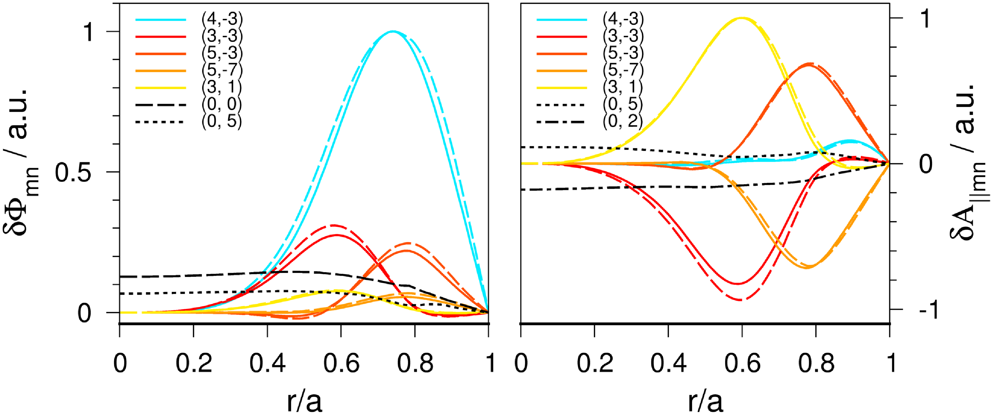
For a comparison of the spatial structures a point in time is chosen in the fully developed linear phase of the GK simulation, e.g. $t\approx 23.7\,\unicode{x03BC} \textrm{s}$
for the
$t\approx 23.7\,\unicode{x03BC} \textrm{s}$
for the $\ell =1,2$
equilibrium at
$\ell =1,2$
equilibrium at $\langle \beta \rangle =0.016$
. As is evident from equations (4.3) and (4.4), only the component of the ideal MHD displacement which is normal to the unperturbed magnetic surfaces is needed for the link to GK. As shown in figure 5, very good agreement is found for the Fourier harmonics of
$\langle \beta \rangle =0.016$
. As is evident from equations (4.3) and (4.4), only the component of the ideal MHD displacement which is normal to the unperturbed magnetic surfaces is needed for the link to GK. As shown in figure 5, very good agreement is found for the Fourier harmonics of $\delta \Phi$
and
$\delta \Phi$
and $\delta A_{\|}$
. In addition to the treatments in MHD and GK, the small deviations may also stem from the usage of different straight-field-line coordinates. In
$\delta A_{\|}$
. In addition to the treatments in MHD and GK, the small deviations may also stem from the usage of different straight-field-line coordinates. In $\mathsf{ EUTERPE}$
the so-called
$\mathsf{ EUTERPE}$
the so-called $\mathsf{PEST}$
coordinates (Grimm et al. Reference Grimm, Greene, Johnson and Killeen1976) are employed, which keep the angle
$\mathsf{PEST}$
coordinates (Grimm et al. Reference Grimm, Greene, Johnson and Killeen1976) are employed, which keep the angle $\varphi$
of the cylindrical coordinates with planar toroidal cuts of the simulation domain. With the coordinates used in
$\varphi$
of the cylindrical coordinates with planar toroidal cuts of the simulation domain. With the coordinates used in $\mathsf{CAS3D}$
, however, the field lines and their orthogonals are straight and, hence, toroidal cuts are non-planar (Boozer Reference Boozer1982). Usually, the resulting differences are small. For clarity in the figure, only the strongest seven out of 597 harmonics are included. In
$\mathsf{CAS3D}$
, however, the field lines and their orthogonals are straight and, hence, toroidal cuts are non-planar (Boozer Reference Boozer1982). Usually, the resulting differences are small. For clarity in the figure, only the strongest seven out of 597 harmonics are included. In $\delta \Phi$
, the resonant harmonic,
$\delta \Phi$
, the resonant harmonic, $(m,n)=(4,-3)$
, is dominant being followed in amplitude by toroidal, tokamak-type side bands,
$(m,n)=(4,-3)$
, is dominant being followed in amplitude by toroidal, tokamak-type side bands, $\Delta (m,n)=\pm (1,0)$
, and helical side bands,
$\Delta (m,n)=\pm (1,0)$
, and helical side bands, $\Delta (m,n)=\pm (1, -4)$
for the four-period stellarator. Due to the discrete, fourfold symmetry of the stellarator, the eigenmodes belonging to different mode families decouple in the MHD stability calculations (Schwab Reference Schwab1993). Therefore, the zonal component,
$\Delta (m,n)=\pm (1, -4)$
for the four-period stellarator. Due to the discrete, fourfold symmetry of the stellarator, the eigenmodes belonging to different mode families decouple in the MHD stability calculations (Schwab Reference Schwab1993). Therefore, the zonal component, $m=n=0$
, does not contribute to the dominantly
$m=n=0$
, does not contribute to the dominantly $(4,-3)$
ideal-MHD perturbation. In contrast to the Fourier structure of
$(4,-3)$
ideal-MHD perturbation. In contrast to the Fourier structure of $\delta \Phi$
, the resonant harmonic of
$\delta \Phi$
, the resonant harmonic of $\delta A_{\|}$
, i.e.
$\delta A_{\|}$
, i.e. $(m,n)=(4,-3)$
, is smaller than the toroidicity- and helicity-induced couplings, i.e.
$(m,n)=(4,-3)$
, is smaller than the toroidicity- and helicity-induced couplings, i.e. $(4,-3)\pm (1,0)$
and (
$(4,-3)\pm (1,0)$
and ( $4,-3)\pm (1,-N_{{\rm p}})$
. This can be understood by a closer look on equations (4.3) and (4.4) employing magnetic coordinates, because then the directional derivatives (
$4,-3)\pm (1,-N_{{\rm p}})$
. This can be understood by a closer look on equations (4.3) and (4.4) employing magnetic coordinates, because then the directional derivatives ( $\boldsymbol{B}\boldsymbol{\cdot} \boldsymbol{\nabla}$
and
$\boldsymbol{B}\boldsymbol{\cdot} \boldsymbol{\nabla}$
and $\boldsymbol{\nabla } s{\,\times\,}\boldsymbol{B}\boldsymbol{\cdot} \boldsymbol{\nabla}$
) are linear differential operators in the magnetic angles with coefficients constant on flux surfaces. Therefore, additionally, this is conveniently done in Fourier space. It is seen that, firstly, the Fourier harmonics of
$\boldsymbol{\nabla } s{\,\times\,}\boldsymbol{B}\boldsymbol{\cdot} \boldsymbol{\nabla}$
) are linear differential operators in the magnetic angles with coefficients constant on flux surfaces. Therefore, additionally, this is conveniently done in Fourier space. It is seen that, firstly, the Fourier harmonics of $\delta \Phi$
only differ from the ones of the MHD normal displacement by a factor depending on the flux label. Secondly, ignoring the variations of
$\delta \Phi$
only differ from the ones of the MHD normal displacement by a factor depending on the flux label. Secondly, ignoring the variations of $B$
for a moment, the harmonics of
$B$
for a moment, the harmonics of $\delta A_{\|}$
are analogously obtained from the Fourier harmonics of
$\delta A_{\|}$
are analogously obtained from the Fourier harmonics of $\boldsymbol \xi \boldsymbol \cdot {\boldsymbol \nabla } s$
, however, multiplied by a factor
$\boldsymbol \xi \boldsymbol \cdot {\boldsymbol \nabla } s$
, however, multiplied by a factor $m\iota +n$
, which approximately vanishes for resonant harmonics.
$m\iota +n$
, which approximately vanishes for resonant harmonics.
Left: normalised temperature (solid black), density (dashed black) and pressure (dashed red) equilibrium profiles of a flat-density scenario; compare figure 3 for the $\eta _{{\rm i,e}}=1$
profiles. Time evolution of the volume-averaged perturbed ion energy flux in normalised units for the
$\eta _{{\rm i,e}}=1$
profiles. Time evolution of the volume-averaged perturbed ion energy flux in normalised units for the $\ell =1,2$
case at
$\ell =1,2$
case at $\langle \beta \rangle =0.02$
(middle) and
$\langle \beta \rangle =0.02$
(middle) and $0.01$
(right). Middle panel:
$0.01$
(right). Middle panel: $\eta _{{\rm i,e}}=1$
(black), flat-density simulation with quad-tree smoothing (red), and without smoothing (cyan). Right panel: simulations including the
$\eta _{{\rm i,e}}=1$
(black), flat-density simulation with quad-tree smoothing (red), and without smoothing (cyan). Right panel: simulations including the $\delta B_{\|}$
-terms (black) and omitting them (red).
$\delta B_{\|}$
-terms (black) and omitting them (red).
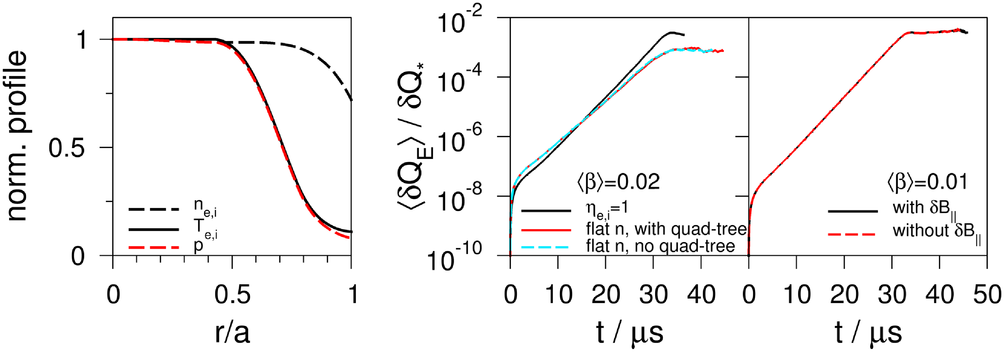
As described in § 2, throughout the present work identical normalised equilibrium temperature and density profiles were used. However, the decomposition of the equilibrium pressure profile into temperature and density profiles is arbitrary. Therefore, in addition to the $\eta_{\rm i,e}=1$
equilibrium profiles, simulations were also done for an
$\eta_{\rm i,e}=1$
equilibrium profiles, simulations were also done for an $\ell =1,2$
equilibrium with the pressure of the
$\ell =1,2$
equilibrium with the pressure of the $\eta _{{\rm i,e}}=1$
case being split into steep equilibrium temperature profiles,
$\eta _{{\rm i,e}}=1$
case being split into steep equilibrium temperature profiles, $T_{\rm e}=T_{\rm i}$
, and flat, but non-uniform equilibrium density profiles,
$T_{\rm e}=T_{\rm i}$
, and flat, but non-uniform equilibrium density profiles, $n_{\rm e}=n_{\rm i}$
, as shown in the left panel of figure 6. As illustrated in the middle panel, the linear-phase growth rate is lower for the flat-density simulation,
$n_{\rm e}=n_{\rm i}$
, as shown in the left panel of figure 6. As illustrated in the middle panel, the linear-phase growth rate is lower for the flat-density simulation, $\gamma =0.16\,(\unicode{x03BC} \textrm{s})^{-1}$
, as compared with the one employing the
$\gamma =0.16\,(\unicode{x03BC} \textrm{s})^{-1}$
, as compared with the one employing the $\eta _{{{\rm e},{\rm i}}}=1$
profiles,
$\eta _{{{\rm e},{\rm i}}}=1$
profiles, $\gamma =0.2\,(\unicode{x03BC} \textrm{s})^{-1}$
. The ideal-MHD stability calculations employing
$\gamma =0.2\,(\unicode{x03BC} \textrm{s})^{-1}$
. The ideal-MHD stability calculations employing $\gamma _{\rm{ h}}=5/3$
, however, find a slightly higher growth rate,
$\gamma _{\rm{ h}}=5/3$
, however, find a slightly higher growth rate, $\gamma =0.22\,(\unicode{x03BC} \textrm{s})^{-1}$
for the flat-density case as compared with the
$\gamma =0.22\,(\unicode{x03BC} \textrm{s})^{-1}$
for the flat-density case as compared with the $\eta _{{\rm i,e}}=1$
case with
$\eta _{{\rm i,e}}=1$
case with $\gamma =0.2\,(\unicode{x03BC} \textrm{s})^{-1}$
. One reason for this may lie in a structural difference between ideal MHD and GK. The MHD force operator includes the equilibrium pressure and its gradient, and the equilibrium density only appears in the kinetic energy acting as a normalisation. Conversely, in GK the density and temperature gradients are both sources of free energy.
$\gamma =0.2\,(\unicode{x03BC} \textrm{s})^{-1}$
. One reason for this may lie in a structural difference between ideal MHD and GK. The MHD force operator includes the equilibrium pressure and its gradient, and the equilibrium density only appears in the kinetic energy acting as a normalisation. Conversely, in GK the density and temperature gradients are both sources of free energy.
Comparative $\mathsf{ EUTERPE}$
simulations including and omitting
$\mathsf{ EUTERPE}$
simulations including and omitting $\delta B_{\|}$
are presented in the right panel of figure 6. With practically identical time traces, coincidence as well in the linear-phase growth rate as in the saturation level is found. Therefore, this term plays a subordinate role only, suggesting that it may be neglected in GK simulations in the regime of MHD proper. Here, the latter is understood as a scenario in which low-
$\delta B_{\|}$
are presented in the right panel of figure 6. With practically identical time traces, coincidence as well in the linear-phase growth rate as in the saturation level is found. Therefore, this term plays a subordinate role only, suggesting that it may be neglected in GK simulations in the regime of MHD proper. Here, the latter is understood as a scenario in which low- $m$
and, therefore, spatially large-scale, modes are dominant. This finding is in line with Kennedy et al. (Reference Kennedy2024), where it was demonstrated that
$m$
and, therefore, spatially large-scale, modes are dominant. This finding is in line with Kennedy et al. (Reference Kennedy2024), where it was demonstrated that $\delta B_{\|}$
has a large impact on hybrid-kinetic-ballooning mode (hybrid-KBM) stability at high
$\delta B_{\|}$
has a large impact on hybrid-kinetic-ballooning mode (hybrid-KBM) stability at high $\beta '$
(e.g.
$\beta '$
(e.g. $\beta '=\textrm{d}\beta /\textrm{d}\rho \approx -0.5$
in their local GK simulations), and a negligible impact at lower
$\beta '=\textrm{d}\beta /\textrm{d}\rho \approx -0.5$
in their local GK simulations), and a negligible impact at lower $\beta '$
. The latter case appears to apply in the simulations presented here, since
$\beta '$
. The latter case appears to apply in the simulations presented here, since $\beta '$
is roughly five times smaller,
$\beta '$
is roughly five times smaller, $\beta '\approx -0.1$
at the location of the strongest pressure gradient,
$\beta '\approx -0.1$
at the location of the strongest pressure gradient, $\rho \approx 0.7$
(figure 3).
$\rho \approx 0.7$
(figure 3).
Sequence of HELIAS equilibria (right panel of figure 1) with variation of the vacuum-field magnetic anti-well, $\mathcal{W}_{{\rm vf}}$
, at fixed
$\mathcal{W}_{{\rm vf}}$
, at fixed $\langle \beta \rangle =0.02$
. Left: time evolution of the volume-averaged perturbed ion energy flux,
$\langle \beta \rangle =0.02$
. Left: time evolution of the volume-averaged perturbed ion energy flux, $\langle \delta Q_{\rm E}\rangle$
, and of the magnetic-field perturbation,
$\langle \delta Q_{\rm E}\rangle$
, and of the magnetic-field perturbation, $\delta B^s$
, both in normalised units. Colours indicate
$\delta B^s$
, both in normalised units. Colours indicate ${\mathcal{W}_{\rm vf}}=0.0057,\,0.01,\,0.017,\,0.03$
(blue, green, cyan, orange). Except for the latter case, the field perturbation is shown by
${\mathcal{W}_{\rm vf}}=0.0057,\,0.01,\,0.017,\,0.03$
(blue, green, cyan, orange). Except for the latter case, the field perturbation is shown by $\boldsymbol{\bullet }$
with the dashed lines meant to guide the eye. Top right: growth rates,
$\boldsymbol{\bullet }$
with the dashed lines meant to guide the eye. Top right: growth rates, $\gamma$
, versus vacuum-field magnetic anti-well,
$\gamma$
, versus vacuum-field magnetic anti-well, $\mathcal{W}_{{\rm vf}}$
. From the GK linear phase
$\mathcal{W}_{{\rm vf}}$
. From the GK linear phase $\boldsymbol{\times }$
and from linearised ideal MHD
$\boldsymbol{\times }$
and from linearised ideal MHD $\boldsymbol{\bullet }$
, with compressible (
$\boldsymbol{\bullet }$
, with compressible ( $\gamma _{\rm{ h}}=5/3$
, red) and nearly incompressible modes (
$\gamma _{\rm{ h}}=5/3$
, red) and nearly incompressible modes ( $\gamma _{\rm h}=10^{-4}$
, cyan). The shading shows the range of the MHD growth rates. Bottom right: frequencies,
$\gamma _{\rm h}=10^{-4}$
, cyan). The shading shows the range of the MHD growth rates. Bottom right: frequencies, $\omega$
, versus
$\omega$
, versus $\mathcal{W}_{{\rm vf}}$
: GK
$\mathcal{W}_{{\rm vf}}$
: GK $\boldsymbol{\times }$
, diamagnetic-drift frequency
$\boldsymbol{\times }$
, diamagnetic-drift frequency $\boldsymbol{\bullet }$
.
$\boldsymbol{\bullet }$
.
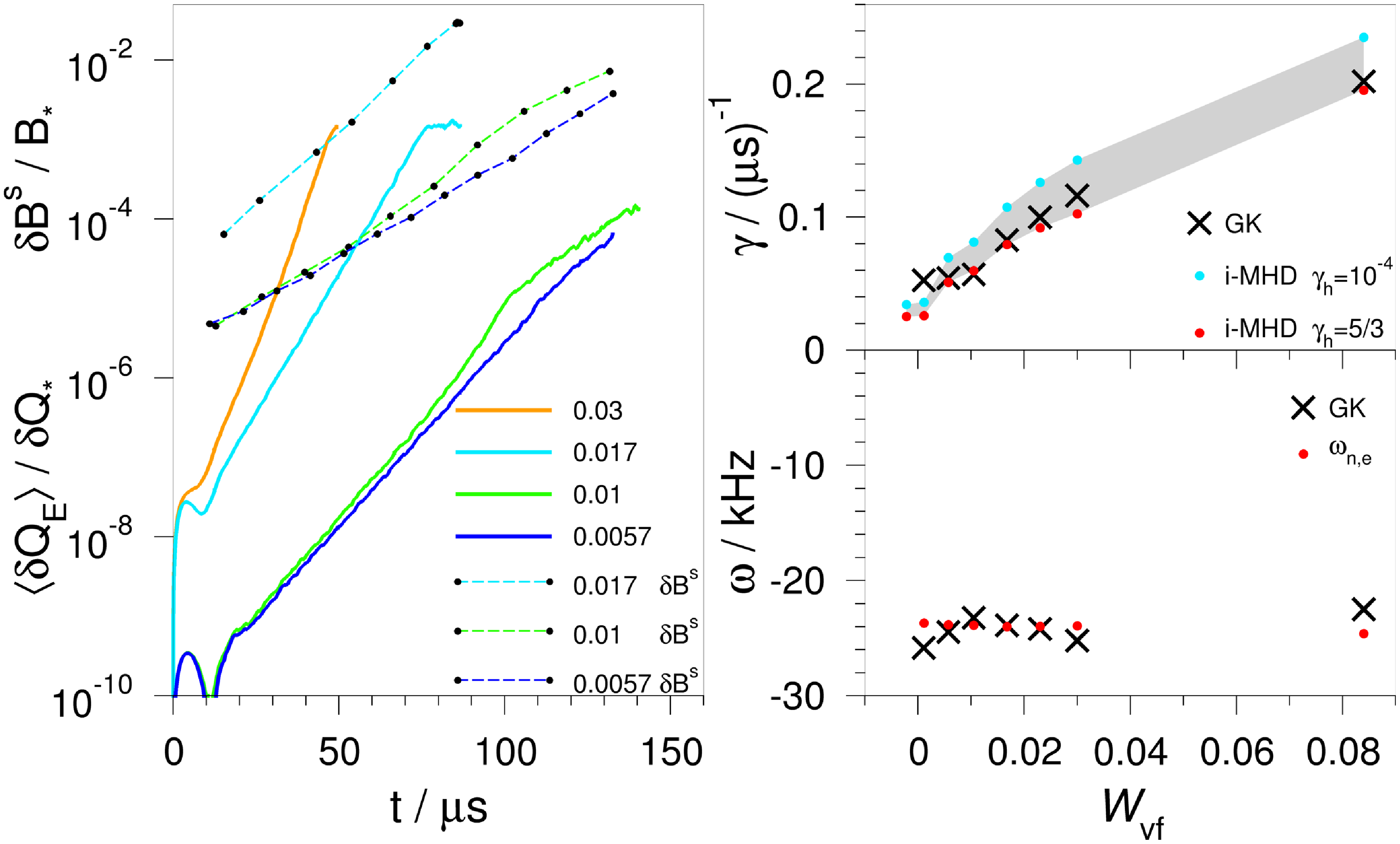
6.1.2. Vacuum-field magnetic-well sequence in HELIAS cases
The set of HELIAS equilibria described in § 2 is even more important because the geometry of the cases is more like W7-X, and information can be obtained on the vacuum-field magnetic well which is used as a series parameter. As shown in figure 7, the linear-ideal-MHD results and the linear-phase findings of the nonlinear GK simulations agree equally well. Both models find that a vacuum-field anti-well corresponds to instability. In units of inverse Alfvén time, equation (2.6), the growth rates increase from $0.015$
to
$0.015$
to $0.033$
for an increase of
$0.033$
for an increase of $\mathcal{W}_{{\rm vf}}$
from
$\mathcal{W}_{{\rm vf}}$
from $0.006$
to
$0.006$
to $0.03$
. As seen before, the electron diamagnetic-drift frequency, equation (6.2), is a good approximation to the frequencies determined by the GK simulations. During a
$0.03$
. As seen before, the electron diamagnetic-drift frequency, equation (6.2), is a good approximation to the frequencies determined by the GK simulations. During a $\mathsf{ EUTERPE}$
simulation the relative magnetic-field perturbation normal to the unperturbed flux surfaces, hence
$\mathsf{ EUTERPE}$
simulation the relative magnetic-field perturbation normal to the unperturbed flux surfaces, hence $\delta B^s$
, is monitored at selected times as illustrated by black bullets in the left panel of figure 7. It is defined by
$\delta B^s$
, is monitored at selected times as illustrated by black bullets in the left panel of figure 7. It is defined by
 \begin{equation} \max _{s,\theta ,\phi }\, \left | \frac {{\boldsymbol \nabla } s}{\mid {\boldsymbol \nabla } s\mid } \boldsymbol \cdot \delta \boldsymbol{B} \right | / B_{\ast }, \end{equation}
with $(s,\theta ,\phi )$
extending over the total simulation domain, i.e. the torus in the present work. The
$(s,\theta ,\phi )$
extending over the total simulation domain, i.e. the torus in the present work. The $\mathsf{ EUTERPE}$
code uses dimensionless quantities,
$\mathsf{ EUTERPE}$
code uses dimensionless quantities, $B_{\ast }$
normalises the magnetic field (Appendix E and table 2). For
$B_{\ast }$
normalises the magnetic field (Appendix E and table 2). For $\langle \beta \rangle =0.02$
and
$\langle \beta \rangle =0.02$
and ${\mathcal{W}_{\rm vf}}=0.017$
(cyan time traces), the relative field perturbation increases to
${\mathcal{W}_{\rm vf}}=0.017$
(cyan time traces), the relative field perturbation increases to $0.013$
at the end of the linear phase,
$0.013$
at the end of the linear phase, $t=76\,\unicode{x03BC} \textrm{s}$
, and saturates at
$t=76\,\unicode{x03BC} \textrm{s}$
, and saturates at $\approx 0.025$
near the end of the simulation,
$\approx 0.025$
near the end of the simulation, $t=86\,\unicode{x03BC} \textrm{s}$
. It should be noted that the magnetic-field perturbation saturates with a time delay as compared with
$t=86\,\unicode{x03BC} \textrm{s}$
. It should be noted that the magnetic-field perturbation saturates with a time delay as compared with $\langle \delta Q_{\rm E}\rangle$
.
$\langle \delta Q_{\rm E}\rangle$
.
6.2. Analysis of the gyrokinetic results
6.2.1. Time evolution of energy fluxes, power spectra and profiles
In addition to the perturbed ion energy flux used in figure 4, figure 8 shows the time evolution of the volume-averaged total ion energy flux ( $\langle Q_{{{\rm E}},0}\rangle$
is the unperturbed flux, which ideally should be zero, but can fluctuate due to particle noise in the PIC method)
$\langle Q_{{{\rm E}},0}\rangle$
is the unperturbed flux, which ideally should be zero, but can fluctuate due to particle noise in the PIC method) $\langle Q_{{{\rm E}}}\rangle =\langle Q_{{{\rm E}},0}\rangle +\langle \delta Q_{{{\rm E}}}\rangle$
, for the plasma-
$\langle Q_{{{\rm E}}}\rangle =\langle Q_{{{\rm E}},0}\rangle +\langle \delta Q_{{{\rm E}}}\rangle$
, for the plasma- $\beta$
scan of
$\beta$
scan of $\ell =1,2$
stellarators. In all
$\ell =1,2$
stellarators. In all $\mathsf{ EUTERPE}$
simulations discussed in this paper, in equilibrium
$\mathsf{ EUTERPE}$
simulations discussed in this paper, in equilibrium $T_{{{\rm e}}}(t_0=0)= T_{{{\rm i}}}(t_0=0)$
and
$T_{{{\rm e}}}(t_0=0)= T_{{{\rm i}}}(t_0=0)$
and $n_{{{\rm e}}}(t_0=0)= n_{{{\rm i}}}(t_0=0)$
, as described in § 2. Although they are independent quantities and independently evolving during the GK simulation, each type of profile (temperature and density) was found to evolve identically for ions and electrons in the scenarios studied here. Therefore, the energy fluxes are the same for electrons and ions (protons) in SI units. Given in gyro-Bohm units, they differ by a factor of
$n_{{{\rm e}}}(t_0=0)= n_{{{\rm i}}}(t_0=0)$
, as described in § 2. Although they are independent quantities and independently evolving during the GK simulation, each type of profile (temperature and density) was found to evolve identically for ions and electrons in the scenarios studied here. Therefore, the energy fluxes are the same for electrons and ions (protons) in SI units. Given in gyro-Bohm units, they differ by a factor of $\sqrt {m_{{\rm p}}/m_{{\rm e}}}$
. For
$\sqrt {m_{{\rm p}}/m_{{\rm e}}}$
. For $\langle \beta \rangle =0.02$
, the maximum of
$\langle \beta \rangle =0.02$
, the maximum of $\langle Q_{{{\rm E}}}\rangle$
is reached at
$\langle Q_{{{\rm E}}}\rangle$
is reached at $\approx 32\,\unicode{x03BC} \textrm{s}$
. For lower plasma pressures the maxima occur at slightly later points in time. Using SI units, it is seen that the saturation levels scale with the plasma pressure. They are comparatively high, e.g.
$\approx 32\,\unicode{x03BC} \textrm{s}$
. For lower plasma pressures the maxima occur at slightly later points in time. Using SI units, it is seen that the saturation levels scale with the plasma pressure. They are comparatively high, e.g. $\approx 300$
in gyro-Bohm units, due to the strongly unstable nature of the
$\approx 300$
in gyro-Bohm units, due to the strongly unstable nature of the $\ell =1,2$
configuration.
$\ell =1,2$
configuration.
Test simulations confirmed the necessity of keeping terms quadratic in the perturbed quantities in the equation of motion for $u_{\|}$
, equation (C.6). Without these so-called magnetic-flutter terms saturation was not reached. The quadratic terms appear where derivatives along directions involving the magnetic field,
$u_{\|}$
, equation (C.6). Without these so-called magnetic-flutter terms saturation was not reached. The quadratic terms appear where derivatives along directions involving the magnetic field, $\boldsymbol{B}+\delta \boldsymbol{B}^{\textrm{GK}}_\perp$
, are applied to perturbation quantities.
$\boldsymbol{B}+\delta \boldsymbol{B}^{\textrm{GK}}_\perp$
, are applied to perturbation quantities.
Time evolution of the volume-averaged total ion energy flux, $\langle Q_{\rm E}\rangle =\langle Q_{\rm E,0}\rangle +\langle \delta Q_{{{\rm E}}}\rangle$
, in SI (left) and gyro-Bohm units (right) in the
$\langle Q_{\rm E}\rangle =\langle Q_{\rm E,0}\rangle +\langle \delta Q_{{{\rm E}}}\rangle$
, in SI (left) and gyro-Bohm units (right) in the $\ell =1,2$
case of figure 4; colours for plasma-
$\ell =1,2$
case of figure 4; colours for plasma- $\beta$
,
$\beta$
, $0.002 \leqslant \langle \beta \rangle \leqslant 0.021$
.
$0.002 \leqslant \langle \beta \rangle \leqslant 0.021$
.
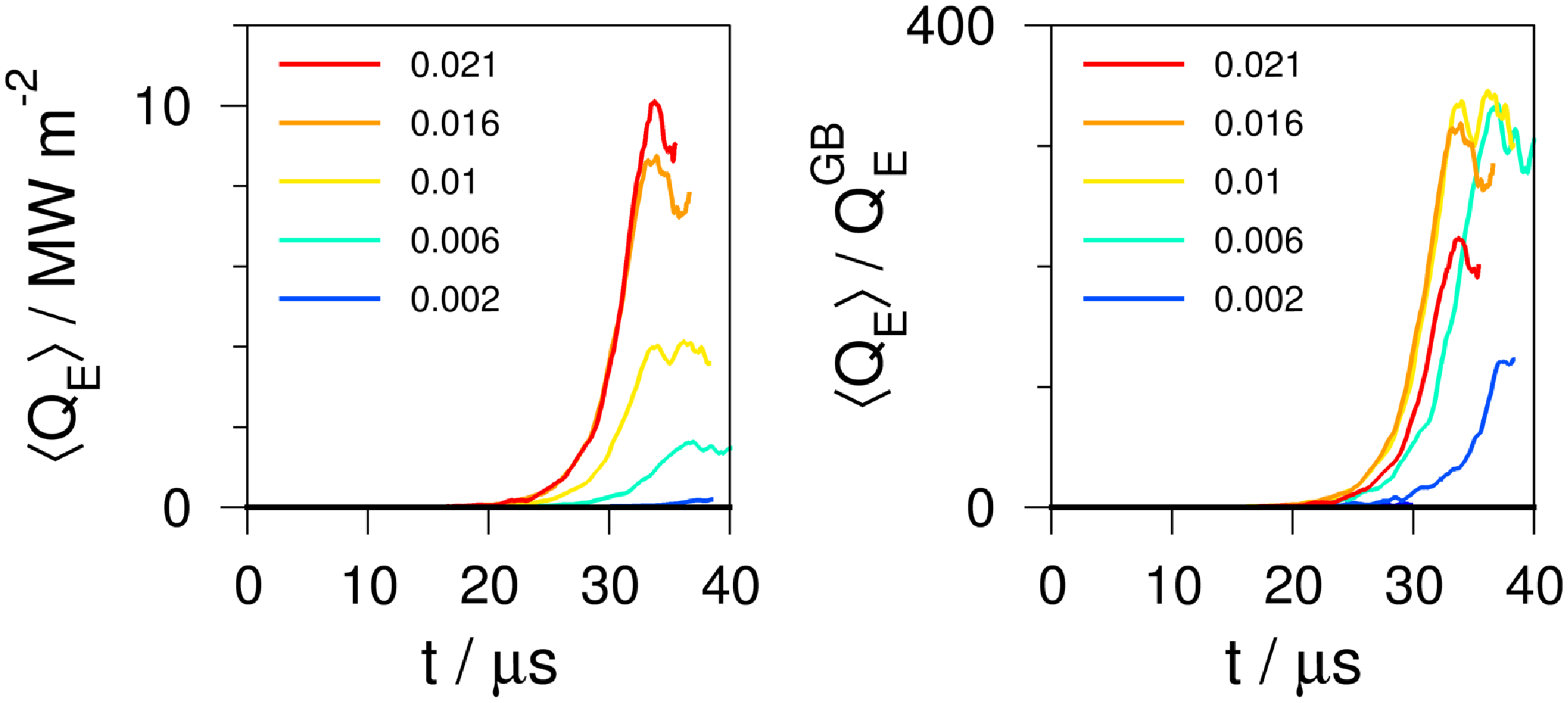
Furthermore, the influence of the so-called quad-tree smoothing for noise control (Sonnendrücker et al. Reference Sonnendrücker, Wacher, Hatzky and Kleiber2015) was studied. For the flat-density $\ell =1,2$
case at
$\ell =1,2$
case at $\langle \beta \rangle =0.02$
, GK simulations were performed with and without the smoothing option. As seen in the middle panel of figure 6, the smoothing procedure leads to an only slightly prolonged saturation phase in this specific case.
$\langle \beta \rangle =0.02$
, GK simulations were performed with and without the smoothing option. As seen in the middle panel of figure 6, the smoothing procedure leads to an only slightly prolonged saturation phase in this specific case.
Time evolution of selected components of the $\delta \Phi$
power spectrum in normalised units,
$\delta \Phi$
power spectrum in normalised units, $\Phi _\ast =(\delta \Phi _\ast )^2$
, shown for HELIAS equilibria at
$\Phi _\ast =(\delta \Phi _\ast )^2$
, shown for HELIAS equilibria at $\langle \beta \rangle =0.02$
,
$\langle \beta \rangle =0.02$
, ${\mathcal{W}_{{\rm vf}}} =0.017$
(left, right) and
${\mathcal{W}_{{\rm vf}}} =0.017$
(left, right) and ${\mathcal{W}_{\mathsf{vf}}}=0.01$
(middle). Left (middle): initialisation of
${\mathcal{W}_{\mathsf{vf}}}=0.01$
(middle). Left (middle): initialisation of $\delta \Phi$
with resonant mode
$\delta \Phi$
with resonant mode $m=4$
,
$m=4$
, $n=-3$
and an admixture of
$n=-3$
and an admixture of $(28,-21)$
at a relative amplitude of 0.001 (0.005); right: initialisation with noise. Colour legend: low-
$(28,-21)$
at a relative amplitude of 0.001 (0.005); right: initialisation with noise. Colour legend: low- $m$
component
$m$
component $(4,-3)$
(red), high-
$(4,-3)$
(red), high- $m$
$m$ $(28,-21)$
(black), zonal component
$(28,-21)$
(black), zonal component $(0,0)$
(cyan). Vertical dashed lines indicate time intervals in which growth rates of the
$(0,0)$
(cyan). Vertical dashed lines indicate time intervals in which growth rates of the $(0,0)$
component are determined by regression as shown by the diagonal dashed lines.
$(0,0)$
component are determined by regression as shown by the diagonal dashed lines.
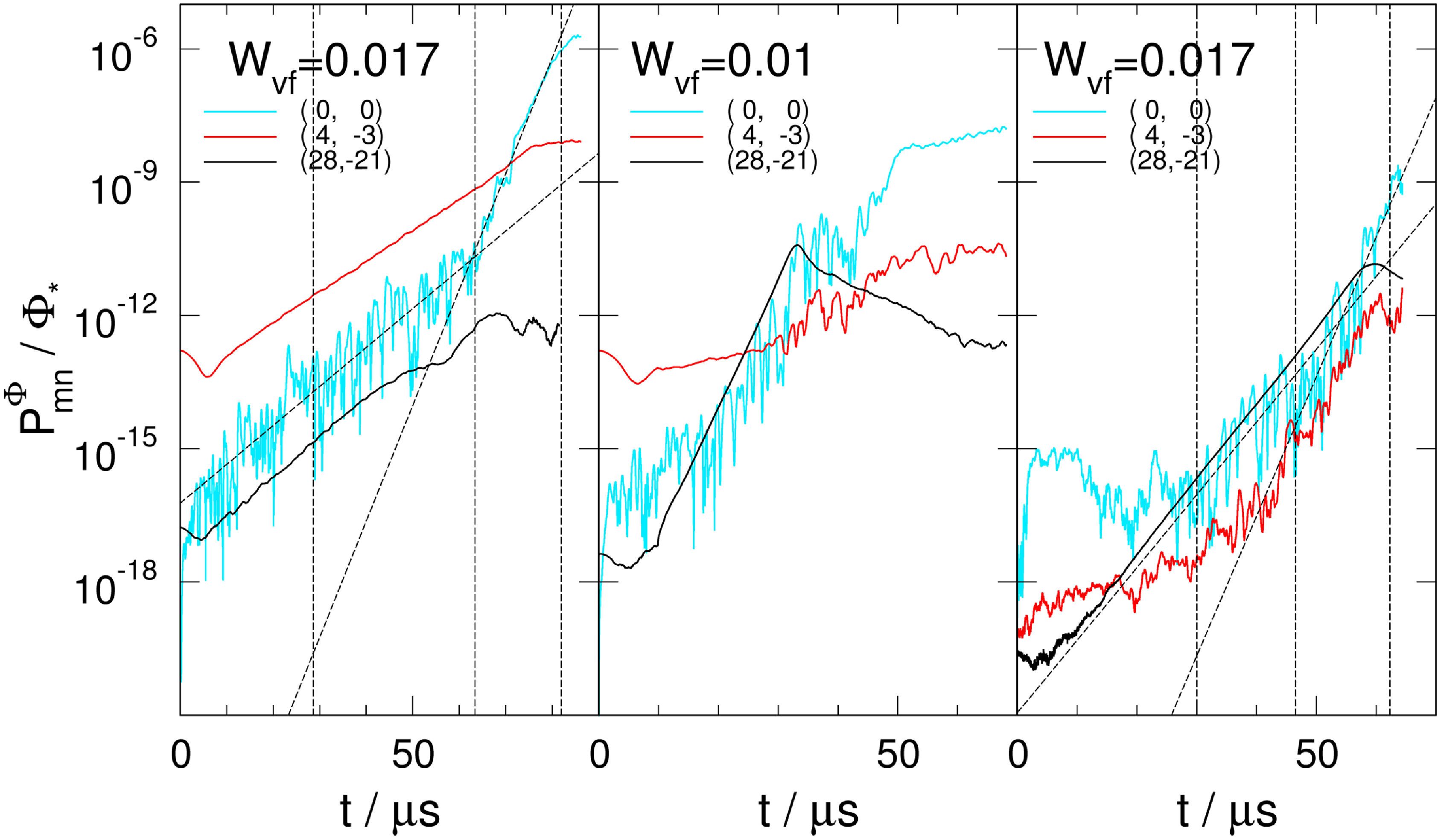
As described in § 6.1, modes detected in the GK simulations are said to have MHD signatures, if they are unstable with dominantly low- $m$
partial modes and, hence, spatially global structures. Furthermore, they have negative GK frequencies, in good agreement with the electron diamagnetic-drift frequency and rotate in the electron diamagnetic direction. An important point of this work was to check how sub-dominant these MHD-like modes are compared with other modes present in the GK simulations. To this end, the initial conditions of
$m$
partial modes and, hence, spatially global structures. Furthermore, they have negative GK frequencies, in good agreement with the electron diamagnetic-drift frequency and rotate in the electron diamagnetic direction. An important point of this work was to check how sub-dominant these MHD-like modes are compared with other modes present in the GK simulations. To this end, the initial conditions of $\delta \Phi$
employed for the
$\delta \Phi$
employed for the $\mathsf{ EUTERPE}$
simulations were varied. The GK results were then analysed using the time traces of the radially averaged power spectra for the Fourier harmonics of
$\mathsf{ EUTERPE}$
simulations were varied. The GK results were then analysed using the time traces of the radially averaged power spectra for the Fourier harmonics of $\delta \Phi$
 \begin{equation} P_{m n}^\Phi (t)= \int \limits _0^1 \big| \delta \Phi _{m n}(\rho ,t) \big|^2\,\textrm{d}\rho. \end{equation}
(The $\mathsf{ EUTERPE}$
code uses normalised quantities which are derived from equilibrium quantities, Appendix E and table 2. A typical normalisation value for
$\mathsf{ EUTERPE}$
code uses normalised quantities which are derived from equilibrium quantities, Appendix E and table 2. A typical normalisation value for $\delta \Phi$
is
$\delta \Phi$
is $\delta \Phi _\ast \approx 1500\,\textrm{V}$
.) By way of example, the four-period HELIAS case at
$\delta \Phi _\ast \approx 1500\,\textrm{V}$
.) By way of example, the four-period HELIAS case at $\langle \beta \rangle =0.02$
and
$\langle \beta \rangle =0.02$
and ${\mathcal{W}_{{\rm vf}}}=0.017$
and
${\mathcal{W}_{{\rm vf}}}=0.017$
and $0.01$
is studied. The respective GK results are summarised in figure 9. In a GK simulation started from noise, i.e. from a randomly set small initial perturbation, the linear phase is dominated by a high-
$0.01$
is studied. The respective GK results are summarised in figure 9. In a GK simulation started from noise, i.e. from a randomly set small initial perturbation, the linear phase is dominated by a high- $m$
perturbation,
$m$
perturbation, $m=28$
,
$m=28$
, $n=-21$
, its side bands, a toroidicity-coupled side band,
$n=-21$
, its side bands, a toroidicity-coupled side band, $(27,-21)$
, being the most important one. Other high-
$(27,-21)$
, being the most important one. Other high- $m$
resonant partial modes, e.g.
$m$
resonant partial modes, e.g. $(24,-18)$
and
$(24,-18)$
and $(22,-17)$
, also contribute, with smaller, but comparable, amplitudes. The respective selected time traces of the total ion energy flux are shown in the right panel of figure 9. With positive frequency, i.e. rotation in the ion-diamagnetic direction and strong amplitudes on the outside of the torus, the high-
$(22,-17)$
, also contribute, with smaller, but comparable, amplitudes. The respective selected time traces of the total ion energy flux are shown in the right panel of figure 9. With positive frequency, i.e. rotation in the ion-diamagnetic direction and strong amplitudes on the outside of the torus, the high- $m$
mode has characteristics of a KBM (Aleynikova et al. Reference Aleynikova, Zocco, Xanthopoulos, Helander and Nührenberg2018; Ishizawa et al. Reference Ishizawa, Imadera, Nakamura and Kishimoto2019). If, as the second choice, the simulation is explicitly initialised at low mode numbers, in this case the resonant
$m$
mode has characteristics of a KBM (Aleynikova et al. Reference Aleynikova, Zocco, Xanthopoulos, Helander and Nührenberg2018; Ishizawa et al. Reference Ishizawa, Imadera, Nakamura and Kishimoto2019). If, as the second choice, the simulation is explicitly initialised at low mode numbers, in this case the resonant $(4,-3)$
, together with a small high-
$(4,-3)$
, together with a small high- $m$
content, here
$m$
content, here $(28,-21)$
at a relative amplitude of 0.001, then the MHD-type low-
$(28,-21)$
at a relative amplitude of 0.001, then the MHD-type low- $m$
mode is dominant in the simulation. The high-
$m$
mode is dominant in the simulation. The high- $m$
component also grows (even at a slightly larger growth rate), but stays subdominant during the entire simulation, because of the much lower initial level. The respective selected time traces are shown in the left panel of figure 9. For these two simulations (left and right panels of figure 9), the time traces of the total ion energy flux are shown in figure 10. The low-
$m$
component also grows (even at a slightly larger growth rate), but stays subdominant during the entire simulation, because of the much lower initial level. The respective selected time traces are shown in the left panel of figure 9. For these two simulations (left and right panels of figure 9), the time traces of the total ion energy flux are shown in figure 10. The low- $m$
MHD-type mode (left panel of figure 9) reaches an
$m$
MHD-type mode (left panel of figure 9) reaches an $\approx 7.5$
times higher maximum of
$\approx 7.5$
times higher maximum of $\langle \delta Q_{{{\rm E}}}\rangle$
than the high-
$\langle \delta Q_{{{\rm E}}}\rangle$
than the high- $m$
KBM (right panel of figure 9). A third choice of initial conditions is illustrated in the middle panel of figure 9. Compared with the low-
$m$
KBM (right panel of figure 9). A third choice of initial conditions is illustrated in the middle panel of figure 9. Compared with the low- $m$
partial mode,
$m$
partial mode, $(4,-3)$
, the relative amplitude of the high-
$(4,-3)$
, the relative amplitude of the high- $m$
partial mode,
$m$
partial mode, $(28,-21)$
, is
$(28,-21)$
, is $0.005$
at the start of the simulation, i.e. initially five times larger than in the simulation depicted in the left panel of figure 9. With this choice, however, the
$0.005$
at the start of the simulation, i.e. initially five times larger than in the simulation depicted in the left panel of figure 9. With this choice, however, the $(28,-21)$
KBM share outweighs the
$(28,-21)$
KBM share outweighs the $(4,-3)$
MHD one at
$(4,-3)$
MHD one at $\approx 25\,\unicode{x03BC} \textrm{s}$
towards the end of the linear phase. This third scenario is also illustrated in figure 11. A sequence of snapshots of
$\approx 25\,\unicode{x03BC} \textrm{s}$
towards the end of the linear phase. This third scenario is also illustrated in figure 11. A sequence of snapshots of $\delta \Phi$
contours on the bean-shaped cross-section shows how the initially MHD-type low-
$\delta \Phi$
contours on the bean-shaped cross-section shows how the initially MHD-type low- $m$
mode transforms into a high-
$m$
mode transforms into a high- $m$
KBM after an intermediate phase, in which the mode is a superposition of both contributions with practically no rotation. The KBM structures get sheared and eventually (while decaying in the saturation phase) become subdominant to zonal structures that dominate the simulation at later times (the latter not shown in figure 11).
$m$
KBM after an intermediate phase, in which the mode is a superposition of both contributions with practically no rotation. The KBM structures get sheared and eventually (while decaying in the saturation phase) become subdominant to zonal structures that dominate the simulation at later times (the latter not shown in figure 11).
Time evolution of the volume-averaged total ion energy flux, $\langle Q_{\rm E}\rangle =\langle Q_{\rm E,0}\rangle +\langle \delta Q_{{{\rm E}}}\rangle$
, in SI (left) and gyro-Bohm units (right) for the simulations shown in the left (low-m) and right (high-m) panels of figure 9; HELIAS case at
$\langle Q_{\rm E}\rangle =\langle Q_{\rm E,0}\rangle +\langle \delta Q_{{{\rm E}}}\rangle$
, in SI (left) and gyro-Bohm units (right) for the simulations shown in the left (low-m) and right (high-m) panels of figure 9; HELIAS case at ${\mathcal{W}_{\rm vf}}=0.017$
and
${\mathcal{W}_{\rm vf}}=0.017$
and $\langle \beta \rangle =0.02$
. The values for the high-m results (black) are magnified by a factor 10.
$\langle \beta \rangle =0.02$
. The values for the high-m results (black) are magnified by a factor 10.
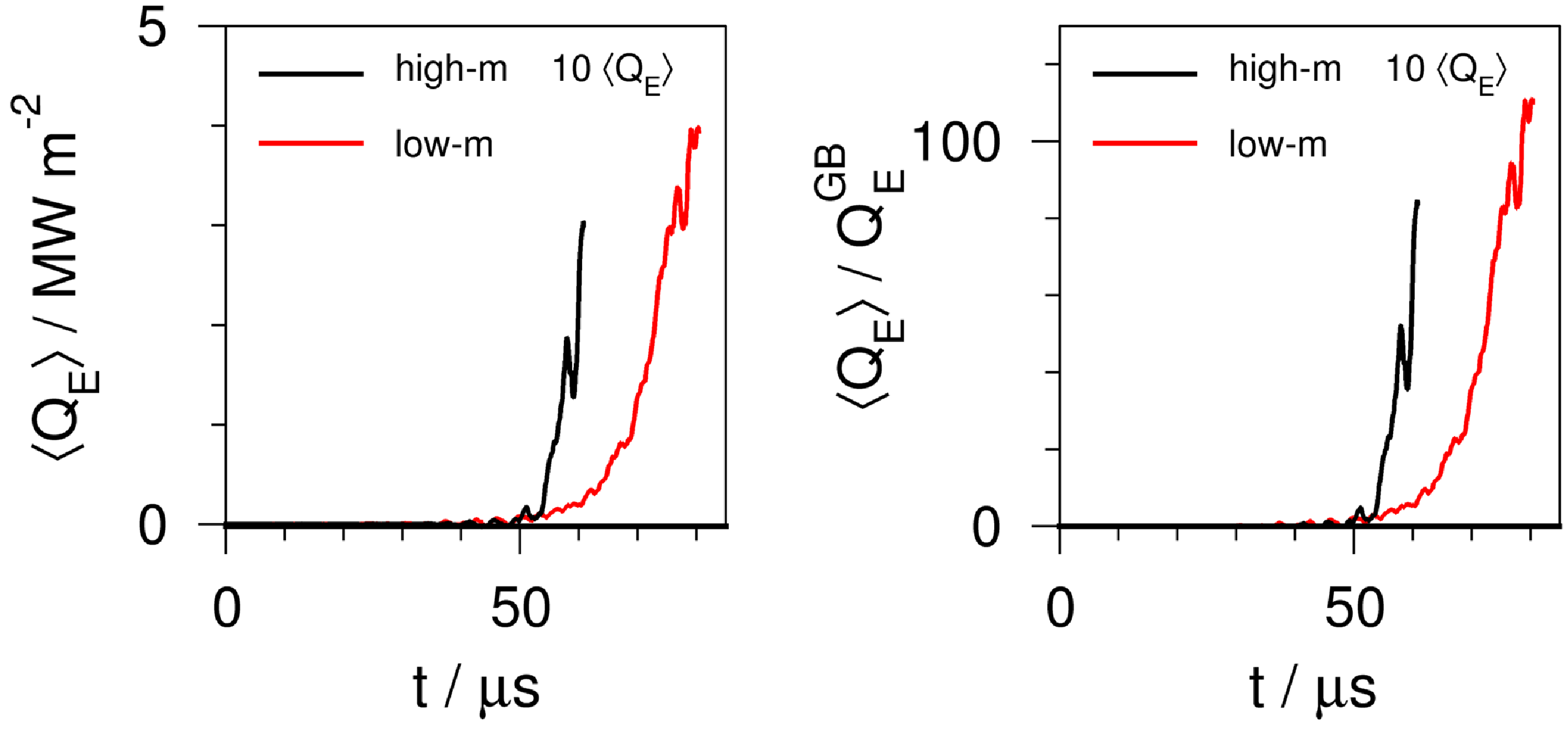
Time evolution of the $\delta \Phi$
contours in normalised units on the bean-shaped cross-section of the HELIAS equilibrium with
$\delta \Phi$
contours in normalised units on the bean-shaped cross-section of the HELIAS equilibrium with ${\mathcal{W}_{\rm vf}}=0.01$
and
${\mathcal{W}_{\rm vf}}=0.01$
and $\langle \beta \rangle =0.02$
. Initialisation of
$\langle \beta \rangle =0.02$
. Initialisation of $\delta \Phi$
with resonant mode
$\delta \Phi$
with resonant mode $m=4$
,
$m=4$
, $n=-3$
and an admixture of
$n=-3$
and an admixture of $m=28$
,
$m=28$
, $n=-21$
with a relative amplitude of 0.005 (see middle panel of figure 9). Time points from left to right:
$n=-21$
with a relative amplitude of 0.005 (see middle panel of figure 9). Time points from left to right: $t/(\unicode{x03BC} \textrm{s})=14,\,21,\,29,\,36$
.
$t/(\unicode{x03BC} \textrm{s})=14,\,21,\,29,\,36$
.
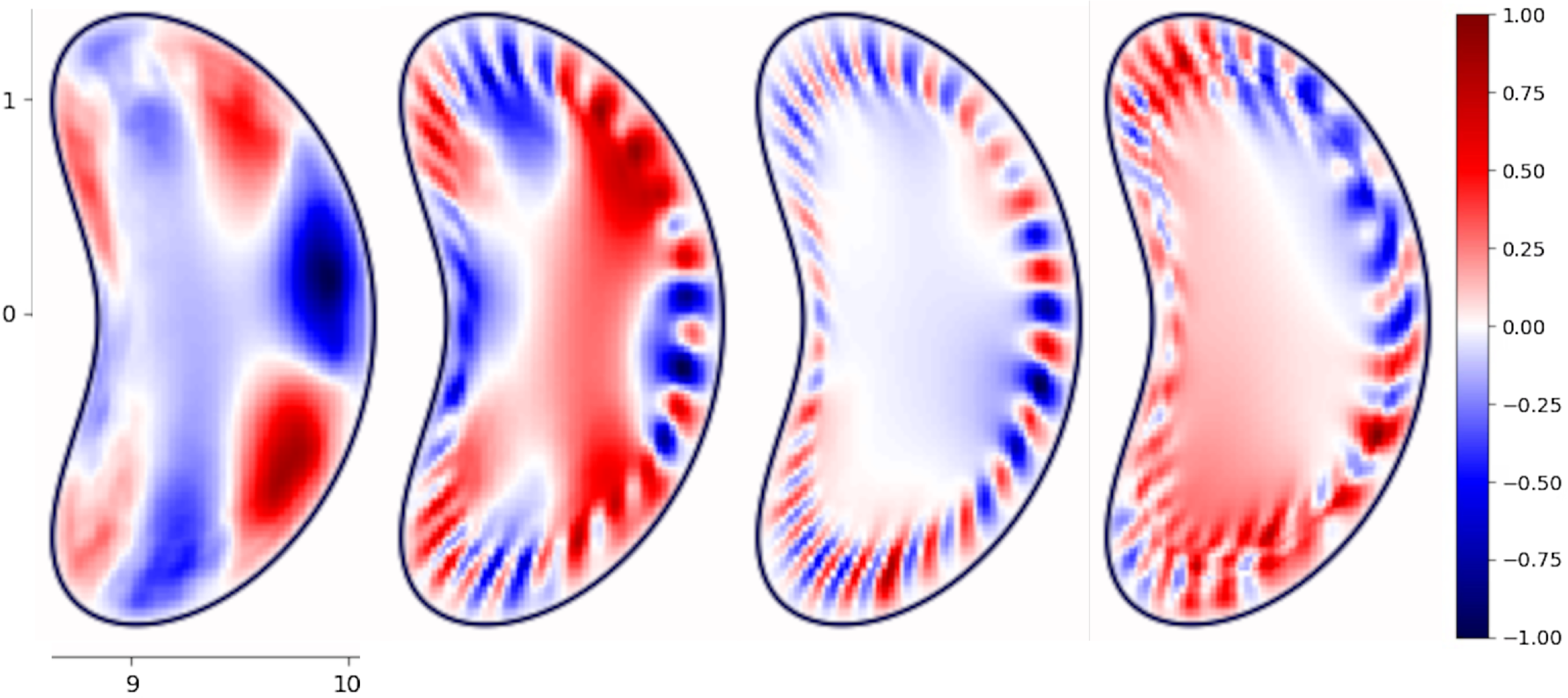
Time evolution of the profiles: ion temperature (coloured dashed) and ion density (coloured solid) in the HELIAS equilibrium at ${\mathcal{W}_{{\rm vf}}}=0.017$
and
${\mathcal{W}_{{\rm vf}}}=0.017$
and $\langle \beta \rangle =0.02$
. The respective electron profiles are shown as black dotted lines. The corresponding changes in the magnetic-field structure are shown in figure 14. Time ranges from
$\langle \beta \rangle =0.02$
. The respective electron profiles are shown as black dotted lines. The corresponding changes in the magnetic-field structure are shown in figure 14. Time ranges from $t=0\,\unicode{x03BC} \textrm{s}$
(black) to
$t=0\,\unicode{x03BC} \textrm{s}$
(black) to $t\approx 82\,\unicode{x03BC} \textrm{s}$
(cyan). Intermediate time instances are shown in red to orange colours,
$t\approx 82\,\unicode{x03BC} \textrm{s}$
(cyan). Intermediate time instances are shown in red to orange colours, $t=61,\,71,\,78\,\unicode{x03BC} \textrm{s}$
.
$t=61,\,71,\,78\,\unicode{x03BC} \textrm{s}$
.
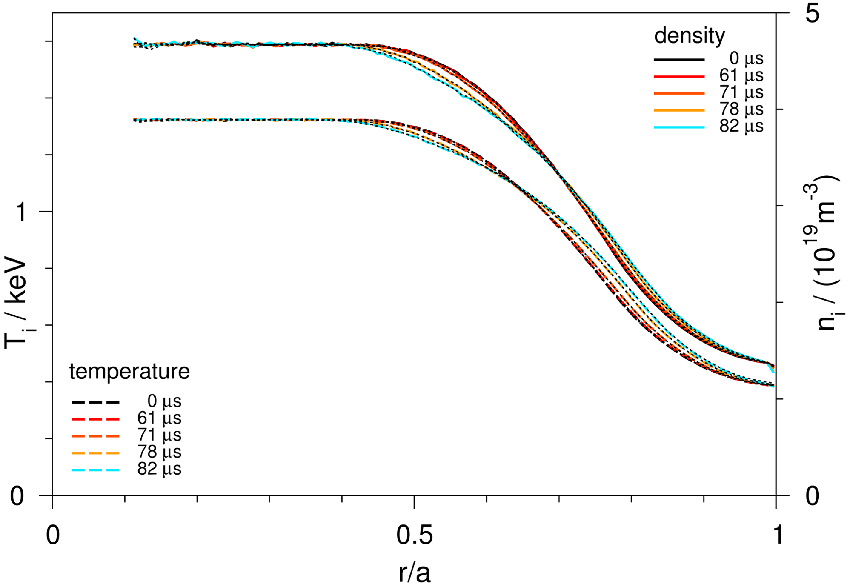
Figure 12 shows the temporal evolution of the temperature and density profiles during the $\mathsf{ EUTERPE}$
simulation for the HELIAS equilibrium at
$\mathsf{ EUTERPE}$
simulation for the HELIAS equilibrium at ${\mathcal{W}_{{\rm vf}}}=0.017$
and
${\mathcal{W}_{{\rm vf}}}=0.017$
and $\langle \beta \rangle =0.02$
, more specifically for a scenario with an unstable, low-
$\langle \beta \rangle =0.02$
, more specifically for a scenario with an unstable, low- $m$
, spatially global and, hence, MHD-type mode. Initially, all normalised profiles are identical,
$m$
, spatially global and, hence, MHD-type mode. Initially, all normalised profiles are identical, $\eta _{{\rm i,e}}=1$
. During the GK simulation, the temperatures and the densities evolve separately, however, identically for ions and electrons, i.e. for all times
$\eta _{{\rm i,e}}=1$
. During the GK simulation, the temperatures and the densities evolve separately, however, identically for ions and electrons, i.e. for all times $T_{{\rm e}}=T_{{\rm i}}$
and
$T_{{\rm e}}=T_{{\rm i}}$
and $n_{{\rm e}}=n_{{\rm i}}$
. Likewise, the ion and electron heat fluxes evolve identically in this scenario. The changes seen in the profiles are rather weak, mostly occurring in the early saturation phase,
$n_{{\rm e}}=n_{{\rm i}}$
. Likewise, the ion and electron heat fluxes evolve identically in this scenario. The changes seen in the profiles are rather weak, mostly occurring in the early saturation phase, $t\lesssim 78\,\unicode{x03BC} \textrm{s}$
. Flattening is seen inside, and, hence, a steepening outside the radial location of the strongest pressure gradient,
$t\lesssim 78\,\unicode{x03BC} \textrm{s}$
. Flattening is seen inside, and, hence, a steepening outside the radial location of the strongest pressure gradient, $\rho \approx 0.7$
.
$\rho \approx 0.7$
.
6.2.2. Properties of the zonal flow
The role of $m=0$
or zonal components is not yet clear and remains under investigation. They immediately appeared in all GK simulations for the MHD-unstable equilibria studied here. The time traces of
$m=0$
or zonal components is not yet clear and remains under investigation. They immediately appeared in all GK simulations for the MHD-unstable equilibria studied here. The time traces of $\langle \delta Q_{{{\rm E}}}\rangle$
, e.g. in figures 4 and 7, show that these simulations could not be continued deep into the saturation phase. A possible reason is seen in the eventual excessive growth of the zonal components during the saturation phase of the other modes, which leads to numerical problems and, consequently, the termination of the simulation. All computational parameters of the GK simulations were carefully checked, e.g. a smaller time step did not solve the problem. The various time traces only cover simulation phases with well-resolved and well-behaved Fourier harmonics of the perturbed potentials,
$\langle \delta Q_{{{\rm E}}}\rangle$
, e.g. in figures 4 and 7, show that these simulations could not be continued deep into the saturation phase. A possible reason is seen in the eventual excessive growth of the zonal components during the saturation phase of the other modes, which leads to numerical problems and, consequently, the termination of the simulation. All computational parameters of the GK simulations were carefully checked, e.g. a smaller time step did not solve the problem. The various time traces only cover simulation phases with well-resolved and well-behaved Fourier harmonics of the perturbed potentials, $\delta \Phi$
and
$\delta \Phi$
and $\delta A_{\|}$
. By way of example, the time traces of the power spectrum of
$\delta A_{\|}$
. By way of example, the time traces of the power spectrum of $\delta \Phi _{0,0}$
are additionally shown in figure 9. In the simulations initialised with noise (right panel), and the low-
$\delta \Phi _{0,0}$
are additionally shown in figure 9. In the simulations initialised with noise (right panel), and the low- $m$
MHD-type perturbation (left panel), the
$m$
MHD-type perturbation (left panel), the $(0,0)$
component oscillates and on average grows at the rate of the dominant mode as indicated by dashed lines. Towards the end of the linear phase, however, the
$(0,0)$
component oscillates and on average grows at the rate of the dominant mode as indicated by dashed lines. Towards the end of the linear phase, however, the $(0,0)$
growth rate changes by a factor of approximately three in the MHD-type regime. In the KBM regime that developed from initial noise, a growth rate twice as high as for the KBM is found. Through this continuing increase of the zonal component the saturation phase ends early, even though the dominant non-zonal modes decrease in amplitude. In the third scenario (middle panel), on the other hand, in which the KBM overtakes the MHD mode, a prolonged saturation phase develops, in which the high-
$(0,0)$
growth rate changes by a factor of approximately three in the MHD-type regime. In the KBM regime that developed from initial noise, a growth rate twice as high as for the KBM is found. Through this continuing increase of the zonal component the saturation phase ends early, even though the dominant non-zonal modes decrease in amplitude. In the third scenario (middle panel), on the other hand, in which the KBM overtakes the MHD mode, a prolonged saturation phase develops, in which the high- $m$
content decreases, and the zonal component only slightly increases.
$m$
content decreases, and the zonal component only slightly increases.
6.2.3. Spatial structures of gyrokinetic perturbation and field-line tracing
The GK simulations proceed from equilibrium calculations assuming nested magnetic surfaces. While an unstable perturbation develops in time, it perturbs the initially intact magnetic geometry too.
Field-line tracing for the GK magnetic field, $\boldsymbol{B}+\delta \boldsymbol{B}^{\textrm{GK}}(t)$
, of the
$\boldsymbol{B}+\delta \boldsymbol{B}^{\textrm{GK}}(t)$
, of the $\ell =1,2$
stellarator, figure 1, with
$\ell =1,2$
stellarator, figure 1, with $\langle \beta \rangle =0.006$
, at
$\langle \beta \rangle =0.006$
, at $t/(\unicode{x03BC} \textrm{s})=0, 32, 35.6, \textrm{and}\,40$
(left to right). Selected field lines in islands are highlighted (right):
$t/(\unicode{x03BC} \textrm{s})=0, 32, 35.6, \textrm{and}\,40$
(left to right). Selected field lines in islands are highlighted (right): $m=4$
(cyan and magenta) and
$m=4$
(cyan and magenta) and $m=9$
(red). The
$m=9$
(red). The $\varphi =0^{\circ }$
cross-section is shown.
$\varphi =0^{\circ }$
cross-section is shown.
Field-line tracing for the GK magnetic field, $\boldsymbol{B}+\delta \boldsymbol{B}^{\mathrm{GK}}(t)$
, of the HELIAS stellarator with
$\boldsymbol{B}+\delta \boldsymbol{B}^{\mathrm{GK}}(t)$
, of the HELIAS stellarator with ${\mathcal{W}_{{\rm vf}}}=0.017$
, and
${\mathcal{W}_{{\rm vf}}}=0.017$
, and $\langle \beta \rangle =0.02$
, at
$\langle \beta \rangle =0.02$
, at $t/(\unicode{x03BC} \textrm{s})=0, 61, \textrm{and}\,71$
(top to bottom). The
$t/(\unicode{x03BC} \textrm{s})=0, 61, \textrm{and}\,71$
(top to bottom). The $\varphi =0^\circ \,{(\textrm{left})\, \textrm{and}}\, 45^\circ$
(right) cross-section are shown. Colours differentiate the field lines. Empty regions near the boundary indicate an island region.
$\varphi =0^\circ \,{(\textrm{left})\, \textrm{and}}\, 45^\circ$
(right) cross-section are shown. Colours differentiate the field lines. Empty regions near the boundary indicate an island region.

For the $\ell =1,2$
equilibrium with
$\ell =1,2$
equilibrium with $\langle \beta \rangle =0.006$
, figure 13 shows the upright-ellipse cross-section at four instances in time, starting with the unperturbed magnetic field. For this simulation the time trace of the perturbed ion energy flux is shown in the left panel of figure 4 (cyan). In the linear phase,
$\langle \beta \rangle =0.006$
, figure 13 shows the upright-ellipse cross-section at four instances in time, starting with the unperturbed magnetic field. For this simulation the time trace of the perturbed ion energy flux is shown in the left panel of figure 4 (cyan). In the linear phase, $t=32\,\unicode{x03BC} \textrm{s}$
, high-
$t=32\,\unicode{x03BC} \textrm{s}$
, high- $m$
islands develop in the outer half of the plasma domain. In the late linear phase,
$m$
islands develop in the outer half of the plasma domain. In the late linear phase, $t=35.6\,\unicode{x03BC} \textrm{s}$
, an
$t=35.6\,\unicode{x03BC} \textrm{s}$
, an $m=4$
island develops and the outer magnetic surfaces begin to ergodise. In the saturation phase, at
$m=4$
island develops and the outer magnetic surfaces begin to ergodise. In the saturation phase, at $t=40\,\unicode{x03BC} \textrm{s}$
, the
$t=40\,\unicode{x03BC} \textrm{s}$
, the $m=4$
island is seen to act in a shielding way, it encloses intact surfaces. Outside the
$m=4$
island is seen to act in a shielding way, it encloses intact surfaces. Outside the $m=4$
island, ergodisation leaves only remnants of
$m=4$
island, ergodisation leaves only remnants of $m=9$
island near the plasma edge.
$m=9$
island near the plasma edge.
Figure 14 shows the intact flux surfaces of the HELIAS equilibrium with $\langle \beta \rangle =0.02$
and
$\langle \beta \rangle =0.02$
and ${\mathcal{W}_{\rm vf}}=0.017$
, and the evolution of the
${\mathcal{W}_{\rm vf}}=0.017$
, and the evolution of the $m=4$
island by two snapshots, at
$m=4$
island by two snapshots, at $t=61\,\unicode{x03BC} \textrm{s}$
and
$t=61\,\unicode{x03BC} \textrm{s}$
and $71\,\unicode{x03BC} \textrm{s}$
. It should be noted here that the equilibrium configuration was deliberately chosen such that no low-order islands exist and the assumption of nested surfaces made by the VMEC code is well justified. With a relative magnetic-field perturbation, equation (6.3), of
$71\,\unicode{x03BC} \textrm{s}$
. It should be noted here that the equilibrium configuration was deliberately chosen such that no low-order islands exist and the assumption of nested surfaces made by the VMEC code is well justified. With a relative magnetic-field perturbation, equation (6.3), of $0.003$
at
$0.003$
at $t=61\,\unicode{x03BC} \textrm{s}$
, a thin
$t=61\,\unicode{x03BC} \textrm{s}$
, a thin $m=4$
island exists and the magnetic surfaces near the plasma boundary wiggle slightly. Near the end of the linear phase, at
$m=4$
island exists and the magnetic surfaces near the plasma boundary wiggle slightly. Near the end of the linear phase, at $t=71\,\unicode{x03BC} \textrm{s}$
and a relative field perturbation of
$t=71\,\unicode{x03BC} \textrm{s}$
and a relative field perturbation of $0.008$
, the surfaces inside the
$0.008$
, the surfaces inside the $m=4$
island are still intact, the island width has increased, and ergodised surfaces fill the outer part of the domain. The ergodisation is, however, not complete, as shown by colouring the distinct field lines. Similar findings are reported for simulations using the nonlinear MHD codes
$m=4$
island are still intact, the island width has increased, and ergodised surfaces fill the outer part of the domain. The ergodisation is, however, not complete, as shown by colouring the distinct field lines. Similar findings are reported for simulations using the nonlinear MHD codes $\mathsf{JOREK}$
(Ramasamy et al. Reference Ramasamy, Aleynikova, Nikulsin, Hindenlang, Holod, Strumberger and Hoelzl2024) and
$\mathsf{JOREK}$
(Ramasamy et al. Reference Ramasamy, Aleynikova, Nikulsin, Hindenlang, Holod, Strumberger and Hoelzl2024) and $\mathsf{M3D-C1}$
(Zhou et al. Reference Zhou, Aleynikova, Liu and Ferraro2024). In figure 10, it is seen that the total ion energy flux strongly increases from
$\mathsf{M3D-C1}$
(Zhou et al. Reference Zhou, Aleynikova, Liu and Ferraro2024). In figure 10, it is seen that the total ion energy flux strongly increases from $t\approx 70\,\unicode{x03BC} \textrm{s}$
. Interestingly, this coincides with the phase of increasing ergodisation of the magnetic field. Future work will continue the study of the magnetic-field structures seen GK simulations in more detail. In addition to the magnetic islands, magnetic surfaces with highly irrational rotational transform (equivalent to Kolmogorov-Arnold-Moser (KAM) surfaces) and near-intact remnants of magnetic surfaces (so-called cantori) are of strong interest (Meiss Reference Meiss1992; Hudson & Breslau Reference Hudson and Breslau2008). While the former are ‘immune’ against field perturbations and prevent complete ergodisation, the latter at least form partial barriers for field lines.
$t\approx 70\,\unicode{x03BC} \textrm{s}$
. Interestingly, this coincides with the phase of increasing ergodisation of the magnetic field. Future work will continue the study of the magnetic-field structures seen GK simulations in more detail. In addition to the magnetic islands, magnetic surfaces with highly irrational rotational transform (equivalent to Kolmogorov-Arnold-Moser (KAM) surfaces) and near-intact remnants of magnetic surfaces (so-called cantori) are of strong interest (Meiss Reference Meiss1992; Hudson & Breslau Reference Hudson and Breslau2008). While the former are ‘immune’ against field perturbations and prevent complete ergodisation, the latter at least form partial barriers for field lines.
7. Summary and outlook
This work brings together GK and linear-ideal-MHD studies for helical-axis $\ell =1,2$
and HELIAS stellarators, the latter being the class of stellarators that also includes the W7-X configuration space. Electromagnetic, nonlinear simulations employing kinetic ions and kinetic electrons with physical mass ratio were performed with the
$\ell =1,2$
and HELIAS stellarators, the latter being the class of stellarators that also includes the W7-X configuration space. Electromagnetic, nonlinear simulations employing kinetic ions and kinetic electrons with physical mass ratio were performed with the $\mathsf{ EUTERPE}$
GK code studying periodicity-breaking perturbations in the full toroidal plasma domain. Such simulations are the first of their kind, to the best knowledge of the authors. The linear-phase GK and the linear-ideal-MHD results were found to be in very good agreement: the growth rates and their dependence on the volume-averaged plasma-
$\mathsf{ EUTERPE}$
GK code studying periodicity-breaking perturbations in the full toroidal plasma domain. Such simulations are the first of their kind, to the best knowledge of the authors. The linear-phase GK and the linear-ideal-MHD results were found to be in very good agreement: the growth rates and their dependence on the volume-averaged plasma- $\beta$
and the vacuum-field magnetic well, as well as the Fourier structure of the perturbed electrostatic and parallel vector potentials of the modes. In particular, this means that both models find that a vacuum-field magnetic anti-well drives instability. It was shown that the parallel magnetic-field perturbation plays no role in the GK simulation of the ideal-MHD-unstable equilibria that were studied in the present work. The inclusion of the magnetic-flutter term was found to be critical for reaching saturation in the GK simulation of the ideal-MHD-unstable equilibria. The sub-dominance of unstable low-mode-number MHD-type modes as compared with KBMs was confirmed in this type of low-shear stellarator. However, as shown by field-line-tracing, low-order island chains driven by the magnetic-field perturbation are expected. The islands enclose intact surfaces and are surrounded by ergodised surfaces in the outer plasma domain. Indications of increasing particle and energy fluxes seen in the present simulations after the onset of ergodisation (potentially leading to a loss of volume of good plasma confinement) will be studied in more detail in future work. In the saturation phase of the GK simulation, a slight flattening of temperature and density profiles was observed. It remains to be investigated whether the turbulent transport or the development of the island and ergodic regions is the cause of this flattening. The continued growth of the zonal-flow component in the saturation phase of the GK simulation will be the focus of future work as well as detailed studies of the magnetic-field structures arising in GK simulations. Similar simulations will evaluate the results of experiments conducted for a configuration with small vacuum-field magnetic anti-well in the OP2.3 operation campaign of W7-X.
$\beta$
and the vacuum-field magnetic well, as well as the Fourier structure of the perturbed electrostatic and parallel vector potentials of the modes. In particular, this means that both models find that a vacuum-field magnetic anti-well drives instability. It was shown that the parallel magnetic-field perturbation plays no role in the GK simulation of the ideal-MHD-unstable equilibria that were studied in the present work. The inclusion of the magnetic-flutter term was found to be critical for reaching saturation in the GK simulation of the ideal-MHD-unstable equilibria. The sub-dominance of unstable low-mode-number MHD-type modes as compared with KBMs was confirmed in this type of low-shear stellarator. However, as shown by field-line-tracing, low-order island chains driven by the magnetic-field perturbation are expected. The islands enclose intact surfaces and are surrounded by ergodised surfaces in the outer plasma domain. Indications of increasing particle and energy fluxes seen in the present simulations after the onset of ergodisation (potentially leading to a loss of volume of good plasma confinement) will be studied in more detail in future work. In the saturation phase of the GK simulation, a slight flattening of temperature and density profiles was observed. It remains to be investigated whether the turbulent transport or the development of the island and ergodic regions is the cause of this flattening. The continued growth of the zonal-flow component in the saturation phase of the GK simulation will be the focus of future work as well as detailed studies of the magnetic-field structures arising in GK simulations. Similar simulations will evaluate the results of experiments conducted for a configuration with small vacuum-field magnetic anti-well in the OP2.3 operation campaign of W7-X.
Acknowledgements
Editor Paolo Ricci thanks the referees for their advice in evaluating this article.
Funding
This work has been carried out within the framework of the EUROfusion Consortium, funded by the European Union via the Euratom Research and Training Programme (Grant Agreement No 101052200 — EUROfusion). Views and opinions expressed are, however, those of the author(s) only and do not necessarily reflect those of the European Union or the European Commission. Neither the European Union nor the European Commission can be held responsible for them. The GK simulations presented in this work were performed on the MARCONI FUSION HPC system at CINECA contributing to the TSVVs Physics of Burning Plasmas and Stellarator Optimization of the EUROfusion work plan 2021-2025 and on the HPC systems Raven and Viper at the Max Planck Computing and Data Facility.
Declaration of interests
The authors report no conflict of interest.
Data availability
The data that support the findings of this article are available upon reasonable request from the authors.
Appendix A. Boundary of HELIAS configurations
In the $\mathsf{VMEC}$
equilibrium code, cylindrical coordinates,
$\mathsf{VMEC}$
equilibrium code, cylindrical coordinates, $R, \varphi , Z$
, are employed with Fourier approximations for
$R, \varphi , Z$
, are employed with Fourier approximations for $R$
and
$R$
and $Z$
. The plasma boundary Fourier coefficients of the HELIAS configuration with marginal vacuum-field well are given in table 1. In the boundary description for the case with
$Z$
. The plasma boundary Fourier coefficients of the HELIAS configuration with marginal vacuum-field well are given in table 1. In the boundary description for the case with ${\mathcal{W}_{{\rm vf}}}=0.03$
several coefficients are different, namely
${\mathcal{W}_{{\rm vf}}}=0.03$
several coefficients are different, namely $R_{0,1}=1.23$
,
$R_{0,1}=1.23$
, $Z_{0,1}=-1.08$
and
$Z_{0,1}=-1.08$
and $R_{1,1}=-Z_{1,1}=-0.185$
. The series of equilibria described in § 2 is obtained by interpolation of the boundary Fourier tables of these two limiting cases. For the
$R_{1,1}=-Z_{1,1}=-0.185$
. The series of equilibria described in § 2 is obtained by interpolation of the boundary Fourier tables of these two limiting cases. For the $\ell =1,2$
case, all
$\ell =1,2$
case, all $m=2$
coefficients (indentation and triangularity) are set to zero, the excursion of the magnetic axis strengthened by setting
$m=2$
coefficients (indentation and triangularity) are set to zero, the excursion of the magnetic axis strengthened by setting $R_{0,1}=1.49$
and
$R_{0,1}=1.49$
and $Z_{0,1}=-1.3434$
. The turning-ellipse coefficients remain at
$Z_{0,1}=-1.3434$
. The turning-ellipse coefficients remain at $-R_{1,1}=Z_{1,1}=0.185$
. Small adjustments of the rotational-transform profile were achieved by e.g. an increase in
$-R_{1,1}=Z_{1,1}=0.185$
. Small adjustments of the rotational-transform profile were achieved by e.g. an increase in $-R_{1,1}=Z_{1,1}$
resulting in a positive shift of
$-R_{1,1}=Z_{1,1}$
resulting in a positive shift of $\iota$
and a decrease in
$\iota$
and a decrease in $R_{2,0}=Z_{2,0}$
which yields stronger shear.
$R_{2,0}=Z_{2,0}$
which yields stronger shear.
Boundary coefficients of the HELIAS configuration with marginal vacuum-field magnetic well. In the rows, the poloidal index $m$
increases, in the columns the toroidal index
$m$
increases, in the columns the toroidal index $n$
.
$n$
.
Appendix B. Plasma potential energy of ideal MHD stability
A multitude of formulations were developed for the energy brought about by the ideal-MHD displacement $\boldsymbol \xi$
in the plasma, this energy being the most important part in the left-hand side of equation (3.2). The following representation, used e.g. by Correa-Restrepo (Reference Correa-Restrepo1978), explicitly separates stabilising and potentially destabilising terms
$\boldsymbol \xi$
in the plasma, this energy being the most important part in the left-hand side of equation (3.2). The following representation, used e.g. by Correa-Restrepo (Reference Correa-Restrepo1978), explicitly separates stabilising and potentially destabilising terms
 \begin{align} W_{\mathrm{plasma}} &=\frac{1}{2}\int _{{\mathsf{V}_{{ P}}}} \! \Big \lbrace B^{-2}|\boldsymbol{B} {\,\times\,} \delta \boldsymbol{B} |^2 + B^{-2}\,|\boldsymbol{B} \boldsymbol \cdot \delta \boldsymbol{B} - \boldsymbol \xi \boldsymbol \cdot {\boldsymbol \nabla } p|^2 + \gamma _{\rm{ h}} \, p\, |\boldsymbol{\nabla} \boldsymbol{\cdot}\boldsymbol{\xi} |^{2} \nonumber \\ &\hphantom {=\tfrac {1}{2}\int _{{\mathsf{V}}_{\mathsf{ P}}} \! \Big \lbrace } +\lbrack (\boldsymbol \xi \boldsymbol \cdot {\boldsymbol \nabla } p)(\boldsymbol \kappa \boldsymbol \cdot {\boldsymbol \xi }^\ast ) +({\boldsymbol \xi }^\ast \boldsymbol \cdot {\boldsymbol \nabla } p)(\boldsymbol \kappa \boldsymbol \cdot \boldsymbol \xi )\rbrack \nonumber \\ &\hphantom {=\tfrac {1}{2}\int _{{\mathsf{V}}_{\mathsf{ P}}} \! \Big \lbrace } - \frac {j_{\|}}{2\,B}\, \lbrack ({\boldsymbol \xi }^\ast {\,\times\,}\boldsymbol{B} ) \boldsymbol \cdot \delta \boldsymbol{B} + (\boldsymbol \xi {\,\times\,}\boldsymbol{B} )\!\boldsymbol \cdot {\delta \boldsymbol{B}}^\ast \rbrack \Big \rbrace \textrm{d} V, \end{align}
where $\delta \boldsymbol{B}$
is as in equation (3.1), the integration extends over the plasma domain and
$\delta \boldsymbol{B}$
is as in equation (3.1), the integration extends over the plasma domain and $\gamma _{\rm h}$
is the ratio of the specific heats. The field-line bending, the field compression and the plasma or fluid compression, in the order of the first line of equation (B.1), always contribute in favour of stability. The curvature,
$\gamma _{\rm h}$
is the ratio of the specific heats. The field-line bending, the field compression and the plasma or fluid compression, in the order of the first line of equation (B.1), always contribute in favour of stability. The curvature, $\boldsymbol \kappa =- \boldsymbol{b}{\,\times\,} ( {\boldsymbol \nabla \,\times\,}\boldsymbol{b}) = (\boldsymbol{b}\!\boldsymbol \cdot {\boldsymbol \nabla })\boldsymbol{b}$
, in combination with the equilibrium pressure gradient, and the equilibrium parallel-current density,
$\boldsymbol \kappa =- \boldsymbol{b}{\,\times\,} ( {\boldsymbol \nabla \,\times\,}\boldsymbol{b}) = (\boldsymbol{b}\!\boldsymbol \cdot {\boldsymbol \nabla })\boldsymbol{b}$
, in combination with the equilibrium pressure gradient, and the equilibrium parallel-current density, $j_{\|} =\boldsymbol{j} \boldsymbol \cdot \boldsymbol{b}$
, may, however, give rise to pressure- and current-driven instabilities and may, therefore, have a detrimental effect on plasma stability.
$j_{\|} =\boldsymbol{j} \boldsymbol \cdot \boldsymbol{b}$
, may, however, give rise to pressure- and current-driven instabilities and may, therefore, have a detrimental effect on plasma stability.
Appendix C. Gyrokinetic equations of motion
For reference, the GK equations of motion are given here in the so-called mixed formulation used in the $\mathsf{ EUTERPE}$
code. For each kinetic marker species, equations of motion are formulated. In this section the subscript for the marker species is omitted for clarity of notation. The scalar perturbed parallel vector potential
$\mathsf{ EUTERPE}$
code. For each kinetic marker species, equations of motion are formulated. In this section the subscript for the marker species is omitted for clarity of notation. The scalar perturbed parallel vector potential $\delta A_{\|}$
is split into a symplectic and a Hamiltonian part
$\delta A_{\|}$
is split into a symplectic and a Hamiltonian part
 \begin{equation} \delta A_{\|} = \delta A_{\|}^{\rm s} + \delta A_{\|}^{\rm h}. \end{equation}
The Hamiltonian part, $\delta A_{\|}^{{\rm h}}$
, is used to define
$\delta A_{\|}^{{\rm h}}$
, is used to define
 \begin{equation} u_{\|} \equiv v_{\|} + \frac {q}{m} \big\langle \delta A_{\|}^{\rm h}\big\rangle ,\end{equation}
with $\langle \cdot \rangle$
denoting the gyro-average in the Appendices C and D. The phase-space Jacobian is
$\langle \cdot \rangle$
denoting the gyro-average in the Appendices C and D. The phase-space Jacobian is
 \begin{equation} B_{\|}^\ast = B + \left [\frac {m}{q}u_{\|} + \big\langle \delta A_{\|}^{\rm s}\big\rangle \right ] \,\boldsymbol{b}\!\boldsymbol \cdot ({\boldsymbol \nabla \,\times\,}\boldsymbol{b}). \end{equation}
With the magnetic moment being a constant of motion, $\dot{\unicode{x03BC}} =0$
, the evolution equation for
$\dot{\unicode{x03BC}} =0$
, the evolution equation for $v_{{\perp }}$
is
$v_{{\perp }}$
is
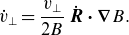 \begin{equation} \dot {v}_{\perp }=\frac {v_{{{\perp }}}}{2 B} \,\dot {\boldsymbol{R}} \boldsymbol \cdot {\boldsymbol \nabla } B. \end{equation}
The equations of motion are
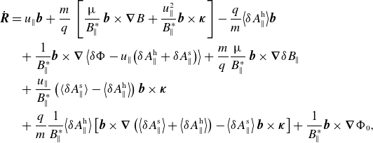 \begin{align} \dot {\boldsymbol{R}} &= u_{\|} \boldsymbol{b} +\frac {m}{q} \, \left [ \frac {\unicode{x03BC} }{B_{\|}^\ast } \, \boldsymbol{b} {\,\times\,} {\boldsymbol \nabla } B + \frac {u_{\|}^{2}}{B_{\|}^\ast } \boldsymbol{b} {\,\times\,} \boldsymbol \kappa \right ] - \frac {q}{m} \big\langle \delta A_{\|}^{{\rm h}}\big\rangle \boldsymbol{b} \nonumber \\ &\hphantom {=} +\frac {1}{B_{\|}^\ast } \boldsymbol{b} {\,\times\,} {\boldsymbol \nabla } \left \langle \delta \Phi - u_{\|} \big( \delta A_{\|}^{{\rm h}} + \delta A_{\|}^{\rm s} \big) \right \rangle + \frac {m}{q}\frac {\unicode{x03BC} }{B_{\|}^\ast } \, \boldsymbol{b}{\,\times\,}{\boldsymbol \nabla }\delta B_{\|} \nonumber \\ &\hphantom {=}+\frac {u_{\|}}{B_{\|}^\ast } \left ( \langle \delta A_{\|}^{{\rm s}}\rangle - \big\langle \delta A_{\|}^{{\rm h}}\big\rangle \right ) \boldsymbol{b} {\,\times\,} \boldsymbol \kappa \nonumber \\ &\hphantom {=} + \frac {q}{m} \frac {1}{B_{\|}^\ast } \big\langle \delta A_{\|}^{{\rm h}}\big\rangle \left [ \boldsymbol{b} {\,\times\,} {\boldsymbol \nabla } \left ( \big\langle \delta A_{\|}^{{\rm s}}\big\rangle + \big\langle \delta A_{\|}^{{\rm h}}\big\rangle \right ) - \big\langle \delta A_{\|}^{{\rm s}}\big\rangle \,\boldsymbol{b}{\,\times\,}\boldsymbol \kappa \right ] + \frac {1}{B_{\|}^\ast } \boldsymbol{b} {\,\times\,} {\boldsymbol \nabla }\Phi _{0} ,\end{align}
and
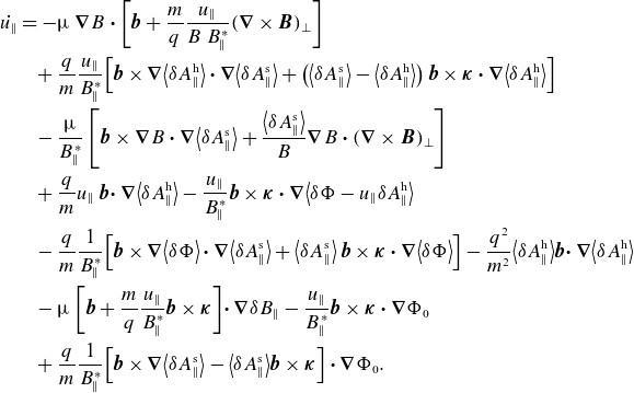 \begin{align} \dot {u_{\|}} &=- \unicode{x03BC} \, {\boldsymbol \nabla } B \boldsymbol \cdot \left[ \boldsymbol{b} + \frac {m}{q} \frac {u_{\|}}{B\, B_{\|}^\ast } ({\boldsymbol \nabla \,\times\,}\boldsymbol{B})_{\perp } \right ] \nonumber \\ &\hphantom {=} + \frac {q}{m} \frac {u_{\|}}{B_{\|}^\ast } \Big[ \boldsymbol{b}{\,\times\,}{\boldsymbol \nabla } \big\langle \delta A_{\|}^{{\rm h}}\big\rangle \boldsymbol \cdot {\boldsymbol \nabla } \big\langle \delta A_{\|}^{\rm s}\big\rangle + \big( \big\langle \delta A_{\|}^{\rm s}\big\rangle - \big\langle \delta A_{\|}^{{\rm h}}\big\rangle \big) \, \boldsymbol{b}{\,\times\,}\boldsymbol \kappa \boldsymbol \cdot {\boldsymbol \nabla } \big\langle \delta A_{\|}^{{\rm h}}\big\rangle \Big] \nonumber \\ &\hphantom {=} - \frac {\unicode{x03BC} }{B_{\|}^\ast } \left[ \boldsymbol{b}{\,\times\,}{\boldsymbol \nabla } B \boldsymbol \cdot {\boldsymbol \nabla } \big\langle \delta A_{\|}^{\rm s}\big\rangle + \frac {\big\langle \delta A_{\|}^{{\rm s}}\big\rangle }{B} {\boldsymbol \nabla } B \boldsymbol \cdot ({\boldsymbol \nabla \,\times\,}\boldsymbol{B} )_{\perp } \right ] \nonumber \\ &\hphantom {=} + \frac {q}{m} u_{\|}\,\boldsymbol{b}\!\boldsymbol \cdot {\boldsymbol \nabla } \big\langle \delta A_{\|}^{\rm h}\big\rangle - \frac {u_{\|}}{B_{\|}^\ast } \boldsymbol{b} {\,\times\,} \boldsymbol \kappa \boldsymbol \cdot {\boldsymbol \nabla } \big\langle \delta \Phi - u_{\|}\delta A_{\|}^{{\rm h}}\big\rangle \nonumber \\ &\hphantom {=} - \frac {q}{m} \frac {1}{B_{\|}^\ast } \Big[ \boldsymbol{b}{\,\times\,}{\boldsymbol \nabla }\big\langle \delta \Phi \big\rangle \boldsymbol \cdot {\boldsymbol \nabla } \big\langle \delta A_{\|}^{\rm s}\big\rangle + \big\langle \delta A_{\|}^{{\rm s}}\big\rangle \, \boldsymbol{b}{\,\times\,}\boldsymbol \kappa \boldsymbol \cdot {\boldsymbol \nabla } \big\langle \delta \Phi \big\rangle \Big] -\frac{q^2}{m^2} \big\langle \delta A_{\|}^{{\rm h}}\big\rangle \boldsymbol{b}\!\boldsymbol \cdot {\boldsymbol \nabla }\big\langle \delta A_{\|}^{{\rm h}}\big\rangle \nonumber \\ &\hphantom {=} - \unicode{x03BC} \left[\boldsymbol{b} + \frac {m}{q} \frac {u_{\|}}{B_{\|}^\ast } \boldsymbol{b}{\,\times\,}\boldsymbol \kappa \right ]\!\boldsymbol \cdot {\boldsymbol \nabla }\delta B_{\|} -\frac {u_{\|}}{B_{\|}^\ast } \boldsymbol{b} {\,\times\,}\boldsymbol \kappa \boldsymbol \cdot {\boldsymbol \nabla } \Phi _{0} \nonumber \\ &\hphantom {=} + \frac {q}{m} \frac {1}{B_{\|}^\ast } \Big[\boldsymbol{b}{\,\times\,} {\boldsymbol \nabla }\big\langle \delta A_{\|}^{{\rm s}}\big\rangle - \big\langle \delta A_{\|}^{{\rm s}}\big\rangle \boldsymbol{b}{\,\times\,}\boldsymbol \kappa \Big] \boldsymbol \cdot {\boldsymbol \nabla }\Phi _{0}. \end{align}
In the above equations, (C.5) and (C.6), an externally given electrostatic potential $\Phi _0$
describes the influence of a radial electric field.
$\Phi _0$
describes the influence of a radial electric field.
Note that in the equations of motion terms quadratic in the perturbed field are retained because they are important for the nonlinear saturation of the modes.
Appendix D. Gyrokinetic weight and field equations in mixed formulation
Magnetic-axis values of equilibrium profiles and normalisations used in the $\mathsf{CAS3D}$
and
$\mathsf{CAS3D}$
and $\mathsf{ EUTERPE}$
simulations for the
$\mathsf{ EUTERPE}$
simulations for the $\ell =1,2$
stellarator of figure 1 with the maximum volume-averaged plasma-
$\ell =1,2$
stellarator of figure 1 with the maximum volume-averaged plasma- $\beta$
used in the calculations.
$\beta$
used in the calculations.
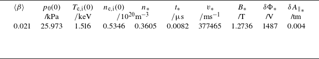
In the following, the subscript $s=\textrm{i, e}$
denotes the marker species. The masses are normalised to the proton mass, the charges to the unsigned elementary charge
$s=\textrm{i, e}$
denotes the marker species. The masses are normalised to the proton mass, the charges to the unsigned elementary charge
 \begin{equation} m_s=\frac {m_{{{\rm i},{\rm e}}}}{m_{{\rm p}}} \quad \hbox{and} \quad q_s=\frac {q_{\rm i,e}}{|e|}. \end{equation}
The weights $w_{s}$
of the PIC marker particles evolve according to
$w_{s}$
of the PIC marker particles evolve according to
 \begin{equation} \dot {w}_{s}=-\Omega _{p} S_{s}, \quad \hbox{with}\quad S_{s}= \dot {\boldsymbol{R}}\!\boldsymbol \cdot {\boldsymbol \nabla } f_{0,s} + \dot {u}_{\|} \,\frac {\partial f_{0,s}}{\partial {v}_{\|}} + \dot {v}_{\perp } \,\frac {\partial f_{0,s}}{\partial v_{\perp }}, \end{equation}
with $\Omega _p$
the marker phase-space volume. The unperturbed distribution functions are
$\Omega _p$
the marker phase-space volume. The unperturbed distribution functions are
 \begin{equation} f_{0,s}= \frac {n_{0s}}{(2 \pi )^{\frac {3}{2}}\, v_{\mathrm{th},s}^{3}} \exp \left (-\frac {-{u_{\|}}^2_s+{v_{{\perp }}^2}_s}{2\, v_{{\rm th},s}^{2}}\right ), \end{equation}
with the thermal velocities given by $v_{\mathrm{th},s}^{2}=T_s/m_s$
. The perturbed electrostatic potential follows from the quasi-neutrality equation
$v_{\mathrm{th},s}^{2}=T_s/m_s$
. The perturbed electrostatic potential follows from the quasi-neutrality equation
 \begin{equation} \sum _{s} q_s\, n_s=0, \quad \quad n_{s}=\langle n_{s} \rangle + \frac {m_s}{q_s}\, {\boldsymbol \nabla \boldsymbol \cdot }\left ( \frac {n_{0s}}{B^{2}} \boldsymbol \nabla _{\!\!\!\bot } \delta \Phi \right ). \end{equation}
Ohm’s law determines the symplectic part of $\delta A_{\|}$
 \begin{equation} \frac {\partial \delta A_{\|}^{{\rm s}}}{\partial t} + \boldsymbol{b}\!\boldsymbol \cdot {\boldsymbol \nabla }\delta \Phi = 0. \end{equation}
For a given symplectic $\delta A_{\|}^{{\rm s}}$
, the Hamiltonian part of
$\delta A_{\|}^{{\rm s}}$
, the Hamiltonian part of $\delta A_{\|}$
is determined by Ampère’s law
$\delta A_{\|}$
is determined by Ampère’s law
 \begin{align} - \frac {1}{\unicode{x03BC} _0} {\boldsymbol \nabla \boldsymbol \cdot } \boldsymbol \nabla _{\!\!\!\bot } \delta A_{\|}^{{\rm h}} + \sum _{s} n_{0s}\, \frac {q_s^2}{m_s}\,\delta A_{\|}^{{\rm h}} &= \sum _{s} \langle {j}_{\|,s} \rangle + \frac {1}{\unicode{x03BC} _0} {\boldsymbol \nabla \boldsymbol \cdot }\boldsymbol \nabla _{\!\!\!\bot } \delta A_{\|}^{{\rm s}}. \end{align}
A pressure balance equation is employed to calculate $\delta B_{\|}$
 \begin{equation} -\frac {B}{\beta _{\mathrm{EU}}}\;\delta B_{\|} = \sum _{s} \delta {p_{{\perp }}}_s, \end{equation}
with the perpendicular perturbed pressure given by
 \begin{equation} \delta {p_{{\perp }}}_{s} = m_s \int \unicode{x03BC} B \,\delta f_s\, B_{\|}^\ast \,\textrm{d} u_{\|}\, \textrm{d}\mu \,\textrm{d}\alpha ,\end{equation}
and the quantity $\beta _{\mathrm{EU}}=(\mu_0\, \textrm{k}_{\rm B}\, n_\ast \, T_\ast )/B_\ast ^2$
. The normalisations, indicated by the subscript
$\beta _{\mathrm{EU}}=(\mu_0\, \textrm{k}_{\rm B}\, n_\ast \, T_\ast )/B_\ast ^2$
. The normalisations, indicated by the subscript $\ast$
, are explained in the Appendix E. The phase-space Jacobian
$\ast$
, are explained in the Appendix E. The phase-space Jacobian $B_{\|}^\ast$
is defined in equation (C.3). The angle
$B_{\|}^\ast$
is defined in equation (C.3). The angle $\alpha$
determines the direction of the gyro-radius vector on the gyro-disc.
$\alpha$
determines the direction of the gyro-radius vector on the gyro-disc.
Appendix E. Normalised units in the
$\mathsf{ EUTERPE}$
code

The $\mathsf{ EUTERPE}$
code employs normalised units. The internal units are
$\mathsf{ EUTERPE}$
code employs normalised units. The internal units are $\Omega _\ast =1/t_\ast =|e|B_{\ast }/m_{{\rm p}}$
, with
$\Omega _\ast =1/t_\ast =|e|B_{\ast }/m_{{\rm p}}$
, with $B_{\ast }$
the average value of the equilibrium magnetic field on the magnetic axis,
$B_{\ast }$
the average value of the equilibrium magnetic field on the magnetic axis, $v_\ast =\rho _\ast \,\Omega _\ast$
for velocities, with
$v_\ast =\rho _\ast \,\Omega _\ast$
for velocities, with $\rho _\ast =\sqrt {{k}_{{\rm B}}\,T_\ast m_{{\rm p}}}/(|e|B_{\ast })$
. The temperature
$\rho _\ast =\sqrt {{k}_{{\rm B}}\,T_\ast m_{{\rm p}}}/(|e|B_{\ast })$
. The temperature $T_\ast$
is the electron temperature at mid minor radius. The densities are normalised to the volume-averaged ion number density,
$T_\ast$
is the electron temperature at mid minor radius. The densities are normalised to the volume-averaged ion number density, $n_\ast =N_{{\rm ph}}/V$
, with
$n_\ast =N_{{\rm ph}}/V$
, with $V$
the volume of the toroidal plasma domain. Derived normalisation parameters are
$V$
the volume of the toroidal plasma domain. Derived normalisation parameters are $\delta \Phi _\ast =\textrm{k}_{{\rm B}}\,T_\ast / |e|$
for the perturbed electrostatic potential and
$\delta \Phi _\ast =\textrm{k}_{{\rm B}}\,T_\ast / |e|$
for the perturbed electrostatic potential and ${\delta A_{\|}}_\ast = \rho _\ast \,B_\ast$
for the perturbed parallel vector potential. The normalisation of the energy fluxes is done via
${\delta A_{\|}}_\ast = \rho _\ast \,B_\ast$
for the perturbed parallel vector potential. The normalisation of the energy fluxes is done via $Q_{{\rm E}\ast }=m_{{\rm p}}\,n_\ast \, v_\ast ^3$
. The transformation to gyro-Bohm units is obtained from
$Q_{{\rm E}\ast }=m_{{\rm p}}\,n_\ast \, v_\ast ^3$
. The transformation to gyro-Bohm units is obtained from $Q_{{\rm E},{\rm s}}^{\mathrm{GB}}=m_s\,n_s \, v_s^3\, (\rho _s/a)^2$
, with
$Q_{{\rm E},{\rm s}}^{\mathrm{GB}}=m_s\,n_s \, v_s^3\, (\rho _s/a)^2$
, with $a$
the effective minor radius of the toroidal plasma, and the subscript
$a$
the effective minor radius of the toroidal plasma, and the subscript $s=\textrm{e or i}$
indicating the particle species. Typical values for the
$s=\textrm{e or i}$
indicating the particle species. Typical values for the $\ell =1,2$
equilibrium of figure 1 are summarised in table 2.
$\ell =1,2$
equilibrium of figure 1 are summarised in table 2.


 Open access