


1. Introduction
Hypersonic flows are characterised by a multitude of complex physical phenomena, including shock waves, thermochemical and thermal non-equilibrium, radiation and plasma formation (Longo, Hannemann & Hannemann Reference Longo, Hannemann and Hannemann2007). Among these, the interaction between shock waves and turbulence plays a central role in determining heat transfer, mixing and aerodynamic stability at low altitudes. Accurately predicting the outcome of such interactions is therefore essential for the design of high-speed vehicles (Settles & Dodson Reference Settles and Dodson1994). The onset of hypersonic flow conditions – often referred to as the hypersonic frontier – arises for Mach numbers exceeding 5. At such high speeds, the associated rise in stagnation enthalpy leads to elevated postshock temperatures, activating internal-energy modes, such as molecular vibration and electronic excitation, that otherwise remain inactive under standard thermodynamic conditions (Clarke Reference Clarke1991). As the stagnation enthalpy increases further, these collisions prove sufficiently energetic to induce dissociation/recombination reactions, and ultimately, ionisation. Although the fundamental molecular physics underpinning these processes has been well understood since the 1960s (Clarke & McChesney Reference Clarke and McChesney1964; Vincenti & Kruger Reference Vincenti and Kruger1965; Zeldovich & Raizer Reference Zeldovich and Raizer1966), their interaction with compressible, turbulent flow structures requires further characterisation.
Shock–turbulence interaction (STI) plays a pivotal role in high-speed aerodynamics, particularly at lower altitudes where the Reynolds numbers are higher and turbulence plays a more prominent role. Such interactions arise, for instance, around the vehicle fuselage or within the intake of scramjet engines (Urzay & Di Renzo Reference Urzay and Di Renzo2021). The characteristics of incoming turbulence – its intensity, length scales and compressibility – can dramatically affect the structure and strength of shock waves, leading to significant changes in heat transfer, aerodynamic drag and overall vehicle stability (Andreopoulos, Agui & Briassulis Reference Andreopoulos, Agui and Briassulis2000). Capturing the evolution of turbulent structures in such flows remains challenging due to extreme gradients in velocity, temperature and density. Under these conditions, the STI physics is further complicated by the presence of strong non-equilibrium effects and large separation of scales. As such, accurate characterisation of STI generally demands the use of high-fidelity, scale-resolving numerical simulations (Lele Reference Lele1994; Martin Reference Martin2007; Pirozzoli Reference Pirozzoli2011) owing to the difficulty in reproducing realistic hypersonic flight conditions in controlled experiments, which are subject to the constraints imposed by facility type and the brevity of test durations (Gu & Olivier Reference Gu and Olivier2020; McManamen et al. Reference McManamen, Donzis, North and Bowersox2021).

Figure 1. Sketch of the interaction of a planar shock wave with an isotropic vorticity–entropy–acoustic field in air at Mach 5, representative of the hypersonic regime. Velocities are presented in the shock reference frame. The variables $u_1$
and
$u_1$
and $u_2$
denote the bulk flow velocities upstream and downstream of the shock,
$u_2$
denote the bulk flow velocities upstream and downstream of the shock, $\xi_s$
the shock displacement,
$\xi_s$
the shock displacement, $\ell$
the characteristic turbulence length scale, and
$\ell$
the characteristic turbulence length scale, and $\ell_T$
the thermochemical non-equilibrium length scale.
$\ell_T$
the thermochemical non-equilibrium length scale.
An idealised configuration for STI is the so-called canonical problem, illustrated in figure 1. This configuration isolates the core physics of the STI by deliberately excluding complex influences such as boundary layers, cross-flows and subsonic regions that may connect flow domains across the shock. It therefore offers a controlled setting for investigating the fundamental mechanisms that mediate STI in both supersonic and hypersonic regimes. The schematic depicts a turbulent upstream flow composed of rotational and dilatational perturbations – characteristic of high-intensity turbulence – and a downstream flow containing rotational, entropic and acoustic disturbances. Behind a shock wave in hypersonic flow, a vibrational relaxation layer forms where vibrational energy modes absorb thermal energy, thereby modifying the postshock conditions (Vincenti & Kruger Reference Vincenti and Kruger1965; Clarke Reference Clarke1991). The thickness of this layer, $\ell _T$
, is set by the vibrational relaxation time and the postshock flow speed. This layer coexists with the viscous dissipation layer of postshock turbulence,
$\ell _T$
, is set by the vibrational relaxation time and the postshock flow speed. This layer coexists with the viscous dissipation layer of postshock turbulence, $\delta _\nu$
, and their ratio defines the vibrational Damköhler number,
$\delta _\nu$
, and their ratio defines the vibrational Damköhler number, ${Da} = \delta _{\nu } / \ell _T$
. Depending on flow conditions (Mach number, pressure, gas composition), the Damköhler number can vary significantly, leading to different coupling regimes between thermochemical relaxation and turbulence dissipation.
${Da} = \delta _{\nu } / \ell _T$
. Depending on flow conditions (Mach number, pressure, gas composition), the Damköhler number can vary significantly, leading to different coupling regimes between thermochemical relaxation and turbulence dissipation.
For weakly turbulent flows, the upstream turbulence is typically modelled as homogeneous and isotropic, consisting of a linear combination of rotational, entropic and acoustic fluctuations (Kovásznay Reference Kovásznay1953). Downstream of the shock, these disturbances are redistributed among the same modal families, but with altered amplitudes and length scales due to interaction with the shock and inter-modal coupling. For analysis of turbulence amplification mechanisms across the shock, linear interaction analysis (LIA) has been established as the principal theoretical framework for analysing STI in the weak-disturbance limit. Originating from the pioneering works of Ribner (Reference Ribner1954a , Reference Ribnerb , Reference Ribner1987), Moore (Reference Moore1953) and Chang (Reference Chang1957), which investigated the shock response to isolated vortical, acoustic and entropic disturbances, respectively, LIA provides closed-form solutions for modal amplification under inviscid, linearised conditions. Since then, the formalism has been extended to account for the transient evolution of postshock disturbances (Wouchuk, Huete Ruiz de Lira & Velikovich Reference Wouchuk, Huete Ruiz de Lira and Velikovich2009; Huete, Velikovich & Wouchuk Reference Huete, Velikovich and Wouchuk2011, Reference Huete, Wouchuk and Velikovich2012b ), binary mixtures (Griffond Reference Griffond2005), thermochemical effects in diatomic species (Huete et al. Reference Huete, Cuadra, Vera and Urzay2021) and in multi-component reacting mixtures (Cuadra Reference Cuadra2023; Cuadra et al. Reference Cuadra, Vera, Di Renzo and Huete2023), weak nonlinearities (Thakare et al. Reference Thakare, Nair and Sinha2022, Reference Thakare, Nair and Sinha2024) and has been incorporated into turbulence modelling frameworks (Sinha, Mahesh & Candler Reference Sinha, Mahesh and Candler2003; Veera & Sinha Reference Veera and Sinha2009; Sinha Reference Sinha2012; Quadros et al. Reference Quadros, Sinha and Larsson2016b ; Vemula & Sinha Reference Vemula and Sinha2017; Sethuraman, Sinha & Larsson Reference Sethuraman, Sinha and Larsson2018).
For fully nonlinear simulations of STI, early studies employing this canonical set-up focused primarily on isotropic vortical turbulence (Lee et al. Reference Lee, Lele and Moin1993, Reference Lee, Lele and Moin1997; Larsson & Lele Reference Larsson and Lele2009; Larsson, Bermejo-Moreno & Lele Reference Larsson, Bermejo-Moreno and Lele2013; Ryu & Livescu Reference Ryu and Livescu2014; Livescu & Ryu Reference Livescu and Ryu2016; Chen & Donzis Reference Chen and Donzis2019, Reference Chen and Donzis2022). These studies confirmed that turbulence is amplified across the shock and that LIA captures the leading-order behaviour of Reynolds stresses and vorticity components for weak disturbances. However, as turbulence intensity increases – often characterised by the turbulent Mach number – compressibility effects ahead of the shock become increasingly important and begin to modify both the structure and evolution of turbulent fluctuations. In hypersonic flows, this compressibility manifests through enhanced dilatational energy, acoustic wave generation and the emergence of shocklet-like structures. Even in the absence of shocks, studies of compressible homogeneous isotropic turbulence (HIT) have shown that dilatational modes significantly alter the small-scale dynamics, intermittency and spectral energy transfer (Wang et al. Reference Wang, Shi, Wang, Xiao, He and Chen2012a ; Jagannathan & Donzis Reference Jagannathan and Donzis2016; Wang et al. Reference Wang, Gotoh and Watanabe2017b ).
As the turbulent flow passes through the shock wave, such compressibility-driven disturbances are further amplified, and the redistribution of energy among vortical, acoustic and entropic modes is consequently modified. This process is highly sensitive to the shock strength, the turbulent Mach number and the relative contribution of dilatational fluctuations (Mahesh et al. Reference Mahesh, Lee, Lele and Moin1995, Reference Mahesh, Lele and Moin1997; Tian et al. Reference Tian, Jaberi, Li and Livescu2017, Reference Tian, Jaberi and Livescu2019; Jamme et al. Reference Jamme, Cazalbou, Torres and Chassaing2002; Grube & Martín Reference Grube and Martín2023). For example, Mahesh et al. (Reference Mahesh, Lee, Lele and Moin1995) investigated the interaction between isotropic acoustic turbulence and a normal shock using both linear theory and direct numerical simulation (DNS), showing that incident acoustic waves generate vorticity and enhance postshock turbulence via baroclinic effects. In a subsequent study, Mahesh, Lele & Moin (Reference Mahesh, Lele and Moin1997) considered upstream turbulence containing both vorticity and entropy fluctuations, demonstrating that positively correlated density–velocity disturbances can further amplify turbulence downstream. Jamme et al. (Reference Jamme, Cazalbou, Torres and Chassaing2002) conducted DNS of STI for moderate shock strengths and varying levels of turbulence intensity. The authors reported that increasing compressibility enhances velocity variances downstream in agreement with linear predictions, although deviations were observed at higher $\mathcal{M}_t$
due to shock-deformation effects. Tian et al. (Reference Tian, Jaberi, Li and Livescu2017, Reference Tian, Jaberi and Livescu2019) extended these efforts by incorporating variable-density turbulence in shock-resolving DNS, observing that density stratification modifies scalar mixing, spectral transfer and postshock flow topology, while confirming that LIA remains accurate for Reynolds stress predictions when sufficient scale separation is present. More recently, Grube & Martín (Reference Grube and Martín2023) performed DNS of STI at Mach numbers up to 4.69, with upstream compressibility levels ranging from 2.7 % to 15 %, focusing specifically on the amplification of the streamwise Reynolds stress component. Their results revealed a clear increase in postshock amplification with both increasing compressibility and shock strength. For the precise simulation conditions, we refer the reader to the original studies, or for a comprehensive overview across a broad parameter range, to our recent review (Cuadra et al. Reference Cuadra, Di Renzo, Hoste, Williams, Vera and Huete2025a
).
$\mathcal{M}_t$
due to shock-deformation effects. Tian et al. (Reference Tian, Jaberi, Li and Livescu2017, Reference Tian, Jaberi and Livescu2019) extended these efforts by incorporating variable-density turbulence in shock-resolving DNS, observing that density stratification modifies scalar mixing, spectral transfer and postshock flow topology, while confirming that LIA remains accurate for Reynolds stress predictions when sufficient scale separation is present. More recently, Grube & Martín (Reference Grube and Martín2023) performed DNS of STI at Mach numbers up to 4.69, with upstream compressibility levels ranging from 2.7 % to 15 %, focusing specifically on the amplification of the streamwise Reynolds stress component. Their results revealed a clear increase in postshock amplification with both increasing compressibility and shock strength. For the precise simulation conditions, we refer the reader to the original studies, or for a comprehensive overview across a broad parameter range, to our recent review (Cuadra et al. Reference Cuadra, Di Renzo, Hoste, Williams, Vera and Huete2025a
).
Despite these advances, a systematic investigation of the role of upstream compressibility and the co-existing vibrational excitation in hypersonic STI remains lacking (Cuadra et al. Reference Cuadra, Di Renzo, Hoste, Williams, Vera and Huete2025a ). To the authors’ knowledge, no DNS study to date has concurrently investigated in the hypersonic regime (i) the redistribution of turbulent kinetic energy (TKE) among velocity components, (ii) the role of upstream compressibility in modulating these components, (iii) the influence of internal-energy excitation under thermal equilibrium conditions (non-negligible at Mach 5 or higher) and (iv) a spectral characterisation of turbulent fluctuations upstream and downstream the shock.
Addressing these absences constitutes the main motivation for the present work. Specifically, we examine the two asymptotic limits of the vibrational Damköhler number in order to assess its influence on STI and on the effective specific heat ratio employed in the Rankine–Hugoniot (RH) relations. The limit ${Da} \to 0$
corresponds to a calorically perfect gas, for which the specific heats ratio remains constant (
${Da} \to 0$
corresponds to a calorically perfect gas, for which the specific heats ratio remains constant ( $\gamma = \text{constant}$
). In contrast, the limit
$\gamma = \text{constant}$
). In contrast, the limit ${Da} \to \infty$
reflects an instantaneous thermochemical adjustment across the shock, such that the adiabatic index changes with temperature,
${Da} \to \infty$
reflects an instantaneous thermochemical adjustment across the shock, such that the adiabatic index changes with temperature, $\gamma (T_2) \ne \gamma (T_1)$
. Intermediate cases, where
$\gamma (T_2) \ne \gamma (T_1)$
. Intermediate cases, where ${Da} \sim 1$
and thermochemical non-equilibrium processes are strongly coupled with postshock turbulence decay (Ghosh & Kerkar Reference Ghosh and Kerkar2022; Williams et al. Reference Williams, Di Renzo and Moin2022, Reference Williams, Di Renzo, Urzay and Moin2024), are beyond the scope of the present work. The main objective is to characterise how different perturbation modes are modified by the shock, in terms of both amplitude and spatial scale. Particular attention is given to the role of upstream turbulence compressibility and shock-induced vibrational excitation, using a combination of LIA and DNS. Analysis on the turbulent spectra shows that both techniques predict broadband amplification of velocity spectra downstream of the shock, using the same turbulent spectra input.
${Da} \sim 1$
and thermochemical non-equilibrium processes are strongly coupled with postshock turbulence decay (Ghosh & Kerkar Reference Ghosh and Kerkar2022; Williams et al. Reference Williams, Di Renzo and Moin2022, Reference Williams, Di Renzo, Urzay and Moin2024), are beyond the scope of the present work. The main objective is to characterise how different perturbation modes are modified by the shock, in terms of both amplitude and spatial scale. Particular attention is given to the role of upstream turbulence compressibility and shock-induced vibrational excitation, using a combination of LIA and DNS. Analysis on the turbulent spectra shows that both techniques predict broadband amplification of velocity spectra downstream of the shock, using the same turbulent spectra input.
The remainder of the paper is organised as follows. Section 2 presents the base-flow configuration and examines the influence of thermochemical equilibrium assumptions on the RH relations over a broad range of shock Mach numbers. Section 3 introduces the LIA formalism, discussing TKE amplification. Section 4 details the generation of compressible HIT using linear forcing, which serves as the upstream inflow for the STI problem at Mach 5. The streamwise evolution of turbulence amplification is then analysed and compared with LIA predictions across several cases in § 5, highlighting the effects of upstream compressibility and departures from calorically perfect gas behaviour. The role of compressibility is further assessed by examining its influence on both preshock and postshock turbulent spectra. Conclusions are summarised in § 6. Appendices A, B and C include mathematical derivations, supplementary spectral results and a verification of the numerical set-up, respectively.
2. Base-flow variables across the shock
Consider first the problem of an undisturbed, normal shock wave propagating into a cold, inviscid and irrotational air stream. In the shock-fixed reference frame, the preshock flow is characterised by the density, pressure, flow velocity and enthalpy denoted, respectively, as $\rho _1$
,
$\rho _1$
, $p_1$
,
$p_1$
, $u_1$
and
$u_1$
and $h_1$
. The corresponding flow variables in the postshock gas are denoted as
$h_1$
. The corresponding flow variables in the postshock gas are denoted as $\rho _2$
,
$\rho _2$
, $p_2$
,
$p_2$
, $u_2$
and
$u_2$
and $h_2$
. With use made of the conservation of mass, momentum and energy across the shock, and noting that the mass flux per unit area remains constant (
$h_2$
. With use made of the conservation of mass, momentum and energy across the shock, and noting that the mass flux per unit area remains constant ( $\rho _1 u_1=\rho _2 u_2$
), the RH relations can be written as
$\rho _1 u_1=\rho _2 u_2$
), the RH relations can be written as
 \begin{equation} p_2 = p_1 + \rho _1 u_1^2\left (1-\dfrac {\rho _1}{\rho _2} \right )\qquad \text{and}\qquad h_2=h_1 +\dfrac {u_1^2}{2} \left [1- \left (\dfrac {\rho _1}{\rho _2}\right )^2\right ]\!. \end{equation}
These equations must be supplemented with the ideal-gas equation of state $p =\rho R_{g} T$
, where
$p =\rho R_{g} T$
, where $T$
is the temperature of the fluid particles and
$T$
is the temperature of the fluid particles and $R_g$
is the gas constant of the mixture. Anticipating that air deviates from the calorically perfect gas approximation in the high-Mach-number regime and that irreversible molecular transformations occur behind the shock, the gas enthalpy must be correspondingly modelled to account for these inelastic processes. In our case, the internal energy
$R_g$
is the gas constant of the mixture. Anticipating that air deviates from the calorically perfect gas approximation in the high-Mach-number regime and that irreversible molecular transformations occur behind the shock, the gas enthalpy must be correspondingly modelled to account for these inelastic processes. In our case, the internal energy $e$
and enthalpy
$e$
and enthalpy $h=e+p/\rho$
are defined to include vibrational effects, and the speed of sound squared by
$h=e+p/\rho$
are defined to include vibrational effects, and the speed of sound squared by
 \begin{equation} c^2 = \left (\dfrac {\partial e}{\partial T}\bigg |_{\rho }\right )^{-1}\left (\dfrac {p}{\rho ^2}\dfrac {\partial p}{\partial T}\bigg |_{\rho }-\dfrac {\partial p}{\partial T}\bigg |_{\rho }\dfrac {\partial e}{\partial \rho }\bigg |_{T}\right )+\dfrac {\partial p}{\partial \rho }\bigg |_{T}, \end{equation}
to be used in the definition of the upstream ${\mathcal M}_1=u_1/c_1$
and downstream
${\mathcal M}_1=u_1/c_1$
and downstream ${\mathcal M}_2=u_2/c_2$
bulk Mach numbers ahead and behind the shock.
${\mathcal M}_2=u_2/c_2$
bulk Mach numbers ahead and behind the shock.
When the incoming flow temperature and Mach number are sufficiently low, the air behaves as a calorically perfect ideal gas with frozen composition, and the enthalpy, internal energy and speed of sound squared are only functions of temperature that can be expressed as $h = \gamma (p/\rho )/(\gamma -1)$
,
$h = \gamma (p/\rho )/(\gamma -1)$
, $e = (p/\rho )/(\gamma -1)$
and
$e = (p/\rho )/(\gamma -1)$
and $c^{2} = \gamma p/\rho$
in terms of the pressure to density ratio
$c^{2} = \gamma p/\rho$
in terms of the pressure to density ratio $p/\rho = R_g T$
. This allows writing of the momentum conservation equation and energy conservation equation in (2.1) with use made of the identities
$p/\rho = R_g T$
. This allows writing of the momentum conservation equation and energy conservation equation in (2.1) with use made of the identities $\rho _1 u_1^2/p_1=\gamma {\mathcal M}_1^2$
and
$\rho _1 u_1^2/p_1=\gamma {\mathcal M}_1^2$
and $u_1^2/h_1=(\gamma -1) {\mathcal M}_1^2$
, respectively.
$u_1^2/h_1=(\gamma -1) {\mathcal M}_1^2$
, respectively.
However, this is found to be inaccurate for preshock Mach numbers exceeding roughly $5$
, i.e. in the hypersonic flow regime. For simplicity in the theoretical description of the thermodynamic properties of the gas, and without significant loss of accuracy, let us consider air as a mixture with volumetric composition of
$5$
, i.e. in the hypersonic flow regime. For simplicity in the theoretical description of the thermodynamic properties of the gas, and without significant loss of accuracy, let us consider air as a mixture with volumetric composition of $79\,\%\,\text{N}_2$
and
$79\,\%\,\text{N}_2$
and $21\,\%\,\text{O}_2$
. As this work is focused on the phenomena associated with incipient hypersonics, only vibrational effects will be considered. Thus, the internal energy of the gas is expressed as a function of temperature using thermodynamic models that account for molecular excitation. In this work, both the LIA and DNS computations use the NASA-9 polynomial fits (McBride Reference McBride2002), which provide accurate temperature-dependent representations of specific heat, enthalpy and entropy over a wide temperature range.
$21\,\%\,\text{O}_2$
. As this work is focused on the phenomena associated with incipient hypersonics, only vibrational effects will be considered. Thus, the internal energy of the gas is expressed as a function of temperature using thermodynamic models that account for molecular excitation. In this work, both the LIA and DNS computations use the NASA-9 polynomial fits (McBride Reference McBride2002), which provide accurate temperature-dependent representations of specific heat, enthalpy and entropy over a wide temperature range.
To illustrate the role of vibrational excitation in a more transparent and analytical form, one can alternatively approximate the internal energy by isolating the vibrational contribution via the harmonic oscillator model (see, e.g. (26)–(27) from Cuadra et al. (Reference Cuadra, Di Renzo, Hoste, Williams, Vera and Huete2025a
)). Combined with the RH relations, these expressions provide a closed system for determining the postshock conditions for a prescribed shock intensity, typically characterised by, but not limited to, the shock Mach number ${\mathcal M}_1$
. If vibrational excitation cannot be adequately captured by the harmonic oscillator model, or the gas undergoes dissociation and/or ionisation processes, the model must instead rely on thermochemical equilibrium solvers.
${\mathcal M}_1$
. If vibrational excitation cannot be adequately captured by the harmonic oscillator model, or the gas undergoes dissociation and/or ionisation processes, the model must instead rely on thermochemical equilibrium solvers.

Figure 2. Inverse normalised RH-slope parameters as a function of the upstream Mach number $\mathcal{M}_1$
for normal shocks propagating in air at
$\mathcal{M}_1$
for normal shocks propagating in air at $T_1 = 300$
K and
$T_1 = 300$
K and $p_1 = 1$
atm.
$p_1 = 1$
atm.
To complete the analysis of the base-flow variables across the shock, the normalised RH-slope parameters
 \begin{equation} \varGamma = u_2^2\dfrac {\partial \rho _2}{\partial p_2}\bigg |_{\rho _1, p_1},\quad \varGamma _\rho = \dfrac {\varGamma }{u_1^2} \dfrac {\partial p_2}{\partial \rho _1}\bigg |_{\rho _2, p_1}\quad \text{and} \quad \varGamma _{\!p} = \varGamma \dfrac {\partial p_2}{\partial p_1}\bigg |_{\rho _1,\rho _2} \end{equation}
are conveniently defined, which will be later used in small-amplitude perturbation analysis. Figure 2 show the variation of these normalised RH-slope parameters as a function of the upstream Mach number $\mathcal{M}_1$
(refer to figure 4a from Cuadra et al. Reference Cuadra, Di Renzo, Hoste, Williams, Vera and Huete2025a
for a broader
$\mathcal{M}_1$
(refer to figure 4a from Cuadra et al. Reference Cuadra, Di Renzo, Hoste, Williams, Vera and Huete2025a
for a broader $\mathcal{M}_1$
range), for normal shocks propagating in air at
$\mathcal{M}_1$
range), for normal shocks propagating in air at $T_1 = 300$
K and
$T_1 = 300$
K and $p_1 = 1$
atm. The dashed, solid, dash-dotted and dotted lines correspond to four thermodynamic models: (i) calorically perfect gas (
$p_1 = 1$
atm. The dashed, solid, dash-dotted and dotted lines correspond to four thermodynamic models: (i) calorically perfect gas ( $\gamma = 1.4$
), (ii) a thermally perfect gas using NASA-9 polynomial fits (
$\gamma = 1.4$
), (ii) a thermally perfect gas using NASA-9 polynomial fits ( $\gamma = \gamma (T)$
), (iii) a thermally perfect gas based on the harmonic oscillator approximation (
$\gamma = \gamma (T)$
), (iii) a thermally perfect gas based on the harmonic oscillator approximation ( $\gamma = \gamma _{\textit{ho}}(T)$
) and (iv) a calorically imperfect gas that accounts for both temperature and composition dependencies (
$\gamma = \gamma _{\textit{ho}}(T)$
) and (iv) a calorically imperfect gas that accounts for both temperature and composition dependencies ( $\gamma = \gamma (T, \boldsymbol {n})$
). Panel (a) depicts
$\gamma = \gamma (T, \boldsymbol {n})$
). Panel (a) depicts $\varGamma$
, which characterises the variation of downstream density across the shock. Panels (b) and (c) display
$\varGamma$
, which characterises the variation of downstream density across the shock. Panels (b) and (c) display $-\varGamma _\rho$
, and
$-\varGamma _\rho$
, and $\varGamma _{\!p}$
, which characterise the influence of upstream density and pressure, respectively, on the downstream state. As the Mach number increases, noticeable deviations from the calorically perfect gas model emerge, particularly beyond
$\varGamma _{\!p}$
, which characterise the influence of upstream density and pressure, respectively, on the downstream state. As the Mach number increases, noticeable deviations from the calorically perfect gas model emerge, particularly beyond $\mathcal{M}_1 \approx 2$
, where vibrational excitation effects start to become significant. The two thermally perfect models yield similar values at moderate Mach numbers, but small discrepancies arise for
$\mathcal{M}_1 \approx 2$
, where vibrational excitation effects start to become significant. The two thermally perfect models yield similar values at moderate Mach numbers, but small discrepancies arise for $\mathcal{M}_1 \gtrsim 5$
, due to the more complete treatment of thermodynamic effects in the NASA-9 polynomials, including vibrational anharmonicity, vibration–rotation coupling and electronic excitation (McBride Reference McBride1992). For the conditions tested, around
$\mathcal{M}_1 \gtrsim 5$
, due to the more complete treatment of thermodynamic effects in the NASA-9 polynomials, including vibrational anharmonicity, vibration–rotation coupling and electronic excitation (McBride Reference McBride1992). For the conditions tested, around $\mathcal{M}_1 = 5$
, considering vibrational excitation is a fair simplification, as it captures the dominant thermodynamic behaviour without the need to account for more complex phenomena, such as dissociation. Lastly, it is worth noting that in the calorically perfect gas model, (2.3) simplifies as
$\mathcal{M}_1 = 5$
, considering vibrational excitation is a fair simplification, as it captures the dominant thermodynamic behaviour without the need to account for more complex phenomena, such as dissociation. Lastly, it is worth noting that in the calorically perfect gas model, (2.3) simplifies as $\varGamma = \mathcal{M}_1^{-2}$
,
$\varGamma = \mathcal{M}_1^{-2}$
, $\varGamma _\rho = -\mathcal{R}^{-1}$
and
$\varGamma _\rho = -\mathcal{R}^{-1}$
and $\varGamma _{\!p} = \mathcal{P}\mathcal{M}^{-2}$
. In the remainder of this work, we focus exclusively on the calorically perfect and thermally perfect (NASA-9) models, as these are the same thermodynamic descriptions employed in both the LIA and the DNSs presented in subsequent sections. Accordingly, for
$\varGamma _{\!p} = \mathcal{P}\mathcal{M}^{-2}$
. In the remainder of this work, we focus exclusively on the calorically perfect and thermally perfect (NASA-9) models, as these are the same thermodynamic descriptions employed in both the LIA and the DNSs presented in subsequent sections. Accordingly, for $\mathcal{M}_1 \gtrsim 5$
, additional thermochemical effects not considered here are expected to play a stronger role, and assessing the applicability of LIA in such regimes is left for future investigations.
$\mathcal{M}_1 \gtrsim 5$
, additional thermochemical effects not considered here are expected to play a stronger role, and assessing the applicability of LIA in such regimes is left for future investigations.
3. Linear interaction analysis
3.1. Mathematical formulation
3.1.1. Preshock perturbations as a composition of mono-frequency modes
The formulation employed in the present study is largely consistent with that of Wouchuk et al. (Reference Wouchuk, Huete Ruiz de Lira and Velikovich2009), Huete et al. (Reference Huete, Cuadra, Vera and Urzay2021), Cuadra et al. (Reference Cuadra, Vera, Di Renzo and Huete2023) and Cuadra (Reference Cuadra2023), in which the upstream flow consisted solely of vortical disturbances. Here, the model is extended to account for density (Huete et al. Reference Huete, Velikovich and Wouchuk2011) and pressure (Huete et al. Reference Huete, Wouchuk and Velikovich2012b ) fluctuations in the upstream flow, associated with acoustic, entropic and vortical disturbances. Furthermore, the effect of vibrational excitation is incorporated through the solution of the base-flow equations in (2.1), using the Combustion Toolbox (Cuadra et al. Reference Cuadra, Huete and Vera2025b , Reference Cuadra, Huete and Vera2026), a general-purpose framework for thermochemical modelling of multi-component mixtures. Among its capabilities, the code can solve problems involving reacting and non-reacting shocks under various gas models. In this work, we adopt a thermally perfect gas model in which vibrational excitation is captured through the NASA-9 polynomial fits (McBride Reference McBride2002) embedded in the toolbox. For a broader analysis in terms of shock intensity, we refer to Cuadra et al. (Reference Cuadra, Di Renzo, Hoste, Williams, Vera and Huete2025a ).
The correlation between the nature of entropic and vorticity disturbances suggests the decomposition of the upstream turbulent flow into two types of waves: the vorticity–entropy wave and the acoustic wave. The former can be expressed as a steady wave function in the absence of diffusive effects, namely
 \begin{align} \delta u_1^r \left ( x, y \right )&= \varepsilon _r \langle c_1\rangle \cos \big (k_x^r x \big )\cos \big (k_y y\big ), \\[-12pt]\nonumber \end{align}
 \begin{align} \delta v_1^r \left ( x, y \right )&= \varepsilon _r \langle c_1\rangle \dfrac {k_x^r}{k_y} \sin \big (k_x^r x \big )\sin \big (k_y y\big ), \\[-12pt]\nonumber \end{align}
 \begin{align} \delta \rho _1^e \left ( x, y \right ) &= \varepsilon _e \langle \rho _1\rangle \cos \big (k_x^r x \big )\cos \big (k_y y\big ); \end{align}
upon application of the divergence-free condition in the velocity field. The acoustic mode, corresponding to isentropic curl-free travelling waves, involves perturbations in the form
 \begin{align} \delta u_1^a \left ( x, y,t \right )&= \varepsilon _a \langle c_1\rangle \cos \left (k_x^a x - \omega _a t\right )\cos \big (k_y y\big ) , \\[-12pt]\nonumber \end{align}
 \begin{align} \delta v_1^a \left ( x, y,t \right )&= -\varepsilon _a \langle c_1\rangle \dfrac {k_y}{k_x^a} \sin \left (k_x^a x - \omega _a t\right )\sin \big (k_y y\big ), \\[-12pt]\nonumber \end{align}
 \begin{align} \delta \rho _1^a \left ( x, y ,t\right ) &= \varepsilon _a \langle \rho _1\rangle \dfrac {\omega _a}{k_x^a} \cos \left (k_x^a x-\omega _a t \right )\cos \big (k_y y\big ) , \\[-12pt]\nonumber \end{align}
 \begin{align} \delta p_1 \left ( x, y,t \right ) &= \varepsilon _a \langle \rho _1 \rangle \langle c_1 \rangle ^2 \dfrac {\omega _a}{k_x^a} \cos \left (k_x^a x-\omega _a t \right )\cos \big (k_y y\big ) . \end{align}
In this formulation, $\langle c_1\rangle$
and
$\langle c_1\rangle$
and $\langle \rho _1\rangle$
denote the mean speed of sound and density in the preshock gas, corresponding to the perturbation-free conditions. The dimensionless parameter
$\langle \rho _1\rangle$
denote the mean speed of sound and density in the preshock gas, corresponding to the perturbation-free conditions. The dimensionless parameter $\varepsilon _r$
denotes the preshock streamwise velocity rotational fluctuation amplitude, assumed to be small in the linear theory,
$\varepsilon _r$
denotes the preshock streamwise velocity rotational fluctuation amplitude, assumed to be small in the linear theory, $\varepsilon _r\ll 1$
. Characterised by a smaller level of intensity, the density-entropic fluctuation amplitude
$\varepsilon _r\ll 1$
. Characterised by a smaller level of intensity, the density-entropic fluctuation amplitude $\varepsilon _e$
and the streamwise velocity-acoustic fluctuation amplitude
$\varepsilon _e$
and the streamwise velocity-acoustic fluctuation amplitude $\varepsilon _a$
are so defined. In Huete et al. (Reference Huete, Wouchuk, Canaud and Velikovich2012a
), the case of the lagged reshock problem – a second time-retarded shock interacting with the turbulence generated by a first shock moving in an entropic turbulent flow – the relation between the rotational and entropic disturbances was determined by the first shock properties. In the case considered in this work, the upstream turbulent flow is dominated by the rotational disturbances, so that
$\varepsilon _a$
are so defined. In Huete et al. (Reference Huete, Wouchuk, Canaud and Velikovich2012a
), the case of the lagged reshock problem – a second time-retarded shock interacting with the turbulence generated by a first shock moving in an entropic turbulent flow – the relation between the rotational and entropic disturbances was determined by the first shock properties. In the case considered in this work, the upstream turbulent flow is dominated by the rotational disturbances, so that $\varepsilon _e$
and
$\varepsilon _e$
and $\varepsilon _a$
are smaller or much smaller than
$\varepsilon _a$
are smaller or much smaller than $\varepsilon _r$
. However, their impact on the postshock turbulent flow is not necessarily negligible, as will be demonstrated later. In real applications, such interrelation between the modes comes from additional effects that have not been considered in the LIA description, such as weak nonlinearities and dissipation effects. Therefore, the relation between the three types of perturbation amplitudes must be externally provided. The numerical turbulence generator, employed later in the DNS study, will be used to compute the relative amplitude of the respective modes ahead of the shock.
$\varepsilon _r$
. However, their impact on the postshock turbulent flow is not necessarily negligible, as will be demonstrated later. In real applications, such interrelation between the modes comes from additional effects that have not been considered in the LIA description, such as weak nonlinearities and dissipation effects. Therefore, the relation between the three types of perturbation amplitudes must be externally provided. The numerical turbulence generator, employed later in the DNS study, will be used to compute the relative amplitude of the respective modes ahead of the shock.
The rotational-entropic perturbation is also characterised by the longitudinal wavenumber $k_x^r$
, which is employed to define the upstream vorticity field, namely
$k_x^r$
, which is employed to define the upstream vorticity field, namely
 \begin{equation} \varpi _{z,1} \left ( x, y \right ) =\varepsilon _r \langle c_1\rangle k_y\left [1+\left (\frac {k_x^r}{k_y}\right )^2 \right ] \cos \big (k_x^r x \big )\sin \big (k_y y\big ). \end{equation}
The acoustic field demands the definition of the corresponding wavenumber $k_x^a$
and frequency
$k_x^a$
and frequency $\omega _a$
, which are related to each other through the sonic dispersion relationship
$\omega _a$
, which are related to each other through the sonic dispersion relationship $\omega _a^2 = c_1^2[ (k_x^a)^2+k_y^2]$
. It is found convenient to define the wave angles
$\omega _a^2 = c_1^2[ (k_x^a)^2+k_y^2]$
. It is found convenient to define the wave angles $k_x^r/k_y=1/|\!\tan \theta ^r|$
and
$k_x^r/k_y=1/|\!\tan \theta ^r|$
and $k_x^a/k_y=1/|\!\tan \theta ^a|$
, which are used later in the analytical computation of the postshock mean values through the corresponding probability density functions. Note that a similar transverse wavenumber
$k_x^a/k_y=1/|\!\tan \theta ^a|$
, which are used later in the analytical computation of the postshock mean values through the corresponding probability density functions. Note that a similar transverse wavenumber $k_y$
is used in both rotational-entropic and acoustic modes. This anticipated condition arises because all types of disturbances are generated through the same source and, therefore, share the main properties of the turbulent spectrum.
$k_y$
is used in both rotational-entropic and acoustic modes. This anticipated condition arises because all types of disturbances are generated through the same source and, therefore, share the main properties of the turbulent spectrum.
To perform the normal mode analysis, it is also found useful to write the upstream perturbation variables in the shock reference frame. For this purpose, let us first define the dimensionless time as $\tau = t k_y c_2$
, so the upstream excitation ahead of the shock translates into constant-amplitude oscillations in the asymptotic long-time regime, where
$\tau = t k_y c_2$
, so the upstream excitation ahead of the shock translates into constant-amplitude oscillations in the asymptotic long-time regime, where
 \begin{equation} \omega _{s}^r= \dfrac {{\mathcal R} {\mathcal M}_2}{\tan \theta ^r} \quad {\text{and}}\quad \omega _{s}^a= \dfrac {{\mathcal R} {\mathcal M}_2}{\tan \theta ^a}\left (1-\dfrac {1}{{\mathcal M}_1\cos \theta ^a}\right ) \end{equation}
refer to the dimensionless oscillation frequencies produced by the upstream rotational-entropic and acoustic modes, respectively. Thus, velocity, density, pressure and vorticity perturbations right ahead of the shock, in terms of the dimensionless time $\tau$
, take the form
$\tau$
, take the form
 \begin{align} \overline {u}_{1s}(\tau )&=\dfrac {\delta u_{1s}}{\varepsilon _r c_1}= \cos {\big(\omega _s^r\tau +\phi _r\big)}+ \dfrac {\varepsilon _a}{\varepsilon _r} \cos {\big(\omega _s^a\tau +\phi _a\big)}, \\[-12pt]\nonumber \end{align}
 \begin{align} \overline {v}_{1s}(\tau )&=\dfrac {\delta v_{1s}}{\varepsilon _r c_1}= \dfrac {k_x^r}{k_y}\sin {\big(\omega _s^r\tau +\phi _r\big)}- \dfrac {k_y}{k_x^a}\dfrac {\varepsilon _a}{\varepsilon _r} \sin {\big(\omega _s^a\tau +\phi _a\big)}, \\[-12pt]\nonumber \end{align}
 \begin{align} \overline {\rho }_{1s}(\tau )&=\dfrac {\delta \rho _{1s}}{\varepsilon _r \rho _1}= \dfrac {\varepsilon _e}{\varepsilon _r}\cos {\big(\omega _s^r\tau +\phi _e\big)}+ \dfrac {\omega _a}{k_x^a}\dfrac {\varepsilon _a}{\varepsilon _r} \cos {\big(\omega _s^a\tau +\phi _a\big)}, \\[-12pt]\nonumber \end{align}
 \begin{align} \overline {p}_{1s}(\tau )&=\dfrac {\delta p_{1s}}{\varepsilon _r \rho _1 c_1^2}= \dfrac {\omega _a}{k_x^a}\dfrac {\varepsilon _a}{\varepsilon _r} \cos {\big(\omega _s^a\tau +\phi _a\big)}, \\[-12pt]\nonumber \end{align}
 \begin{align} \overline {\varpi }_{1s}(\tau )&=\dfrac {\varpi _{1s}}{\varepsilon _r k_y c_1}= \left [1+\left (\frac {k_x^r}{k_y} \right )^2\right ]\cos {\big(\omega _s^r\tau +\phi _r\big)}, \end{align}
where the average symbol brackets $\langle \boldsymbol{\cdot }\rangle$
have been omitted for clarity. In writing (3.5),
$\langle \boldsymbol{\cdot }\rangle$
have been omitted for clarity. In writing (3.5), $\phi _r$
,
$\phi _r$
, $\phi _e$
and
$\phi _e$
and $\phi _a$
denote the phases of the rotational, entropic and acoustic modes, respectively, and the subscript
$\phi _a$
denote the phases of the rotational, entropic and acoustic modes, respectively, and the subscript $1s$
defines upstream (subscript
$1s$
defines upstream (subscript $1$
) disturbances at the shock (subscript
$1$
) disturbances at the shock (subscript $s$
) location.
$s$
) location.
3.1.2. Postshock perturbations for dual-frequency composition modes
Once the upstream conditions are determined, the next step is to obtain the postshock properties for the different perturbation modes. In a system of reference moving with the shock front immediately downstream from the perturbed shock surface (subscript $2$
), a corresponding set of perturbations is generated
$2$
), a corresponding set of perturbations is generated
 \begin{align} \overline {u}_{2s}(\tau )&=\dfrac {\delta u_{2s}}{\varepsilon _r c_2}= \big({\mathcal U}_r^r+{\mathcal U}_a^r\big) \cos {\big(\omega _s^r\tau +\phi _r\big)}+ \big({\mathcal U}_r^a+{\mathcal U}_a^a\big)\cos {\big(\omega _s^a\tau +\phi _a\big)}, \\[-12pt]\nonumber \end{align}
 \begin{align} \overline {v}_{2s}(\tau )&=\dfrac {\delta v_{2s}}{\varepsilon _r c_2}=\big({\mathcal V}_r^r+{\mathcal V}_a^r\big)\sin {\big(\omega _s^r\tau +\phi _r\big)} + \big({\mathcal V}_r^a+{\mathcal V}_a^a\big) \sin {\big(\omega _s^a\tau +\phi _a\big)}, \\[-12pt]\nonumber \end{align}
 \begin{align} \overline {\rho }_{2s}(\tau )&=\dfrac {\delta \rho _{2s}}{\varepsilon _r \rho _2}=\big({\mathcal D}_e^r+{\mathcal D}_a^r\big)\cos {\big(\omega _s^r\tau +\phi _e\big)}+ \big({\mathcal D}_e^a+{\mathcal D}_a^a\big)\cos {\big(\omega _s^a\tau +\phi _a\big)}, \\[-12pt]\nonumber \end{align}
 \begin{align} \overline {p}_{2s}(\tau )&=\dfrac {\delta p_{2s}}{\varepsilon _r \rho _2 c_2^2}={\mathcal P}_a^r\cos {\big(\omega _s^r\tau +\phi _e\big)}+ {\mathcal P}_a^a\cos {\big(\omega _s^a\tau +\phi _a\big)}, \\[-12pt]\nonumber \end{align}
 \begin{align} \overline {\varpi }_{2s}(\tau )&=\dfrac {\varpi _{2s}}{\varepsilon _r k_y c_2}= {\mathcal O}_r^r\cos {\big(\omega _s^r\tau +\phi _r\big)+ \mathcal O}_r^a\cos {\big(\omega _s^a\tau +\phi _a\big)}. \end{align}
The postshock mode amplitudes ${\mathcal U}_{r,a}^{r,a}$
,
${\mathcal U}_{r,a}^{r,a}$
, ${\mathcal V}_{r,a}^{r,a}$
,
${\mathcal V}_{r,a}^{r,a}$
, ${\mathcal D}_{e,a}^{r,a}$
,
${\mathcal D}_{e,a}^{r,a}$
, ${\mathcal P}_{a}^{r,a}$
and
${\mathcal P}_{a}^{r,a}$
and ${\mathcal O}_{r}^{r,a}$
are unknowns functions of
${\mathcal O}_{r}^{r,a}$
are unknowns functions of $\theta ^r$
and
$\theta ^r$
and $\theta ^a$
to be determined. Note that in (3.5) and (3.6), the transverse coordinate dependence is omitted,
$\theta ^a$
to be determined. Note that in (3.5) and (3.6), the transverse coordinate dependence is omitted, $\sim\! \cos (k_y y)$
for the longitudinal and
$\sim\! \cos (k_y y)$
for the longitudinal and $\sim\! \sin (k_y y)$
for the transverse velocity field, as it is not affected by the shock passage due to the periodic symmetry in the transverse direction. To distinguish between the different contributions, the subscripts
$\sim\! \sin (k_y y)$
for the transverse velocity field, as it is not affected by the shock passage due to the periodic symmetry in the transverse direction. To distinguish between the different contributions, the subscripts $r,e,a$
refer to the nature of the downstream perturbation, rotational, entropic or acoustic, respectively, while the superscripts
$r,e,a$
refer to the nature of the downstream perturbation, rotational, entropic or acoustic, respectively, while the superscripts $r,a$
refer to the nature of the upstream mode generating the corresponding perturbation, rotational entropic and acoustic, respectively. As such, the rotational streamwise amplitude
$r,a$
refer to the nature of the upstream mode generating the corresponding perturbation, rotational entropic and acoustic, respectively. As such, the rotational streamwise amplitude ${\mathcal U}_{r}(\theta ^r,\theta ^a)$
is conveniently decomposed into components associated with the upstream rotational-entropic wave
${\mathcal U}_{r}(\theta ^r,\theta ^a)$
is conveniently decomposed into components associated with the upstream rotational-entropic wave ${\mathcal U}_{r}^r={\mathcal U}_{r}^r(\theta ^r)$
and the acoustic mode
${\mathcal U}_{r}^r={\mathcal U}_{r}^r(\theta ^r)$
and the acoustic mode ${\mathcal U}_{r}^a= {\mathcal U}_{r}^a(\theta ^a)$
, with the superposition of modes rendering
${\mathcal U}_{r}^a= {\mathcal U}_{r}^a(\theta ^a)$
, with the superposition of modes rendering ${\mathcal U}_{r}={\mathcal U}_{r}^r+{\mathcal U}_{r}^a$
. Likewise,
${\mathcal U}_{r}={\mathcal U}_{r}^r+{\mathcal U}_{r}^a$
. Likewise, ${\mathcal U}_{a}(\theta ^r,\theta ^a)={\mathcal U}_{a}^r(\theta ^r)+{\mathcal U}_{a}^a(\theta ^a)$
,
${\mathcal U}_{a}(\theta ^r,\theta ^a)={\mathcal U}_{a}^r(\theta ^r)+{\mathcal U}_{a}^a(\theta ^a)$
, ${\mathcal D}_{e}(\theta ^r,\theta ^a)={\mathcal D}_{e}^r(\theta ^r)+{\mathcal D}_{e}^a(\theta ^a)$
, and so on.
${\mathcal D}_{e}(\theta ^r,\theta ^a)={\mathcal D}_{e}^r(\theta ^r)+{\mathcal D}_{e}^a(\theta ^a)$
, and so on.
In the compressed gas reference frame, $x_c=x-(u_1-u_2)t$
, the rotational-entropic disturbances remain frozen (steady functions) to the fluid particles, while acoustic perturbations propagate governed by the corresponding sound wave equation
$x_c=x-(u_1-u_2)t$
, the rotational-entropic disturbances remain frozen (steady functions) to the fluid particles, while acoustic perturbations propagate governed by the corresponding sound wave equation
 \begin{equation} \dfrac {\partial ^2\overline {p}_2}{\partial \tau ^2}=\dfrac {\partial ^2\overline {p}_2}{\partial \overline {x}_c^2}-\overline {p}, \end{equation}
where $\overline {x}_c=k_y x_c$
, thereby behaving similar to upstream disturbances described in (3.2d
). To compute the long-time amplitudes of the different modes, the perturbed RH equations must be employed, along with the linearised Euler equations. An additional condition associated with the shock supporting mechanism is needed; in this case, as usual, the isolated shock boundary condition is employed far downstream of the shock. Therefore, all disturbances are generated at the shock front and conveyed (rotational entropic) or radiated (acoustic) downstream.
$\overline {x}_c=k_y x_c$
, thereby behaving similar to upstream disturbances described in (3.2d
). To compute the long-time amplitudes of the different modes, the perturbed RH equations must be employed, along with the linearised Euler equations. An additional condition associated with the shock supporting mechanism is needed; in this case, as usual, the isolated shock boundary condition is employed far downstream of the shock. Therefore, all disturbances are generated at the shock front and conveyed (rotational entropic) or radiated (acoustic) downstream.
The boundary condition at the shock front is derived from the linearised RH jump conditions assuming that (a) the thickness of the vibrational non-equilibrium region $\ell _T$
is much smaller than the inverse of the transverse wavenumber
$\ell _T$
is much smaller than the inverse of the transverse wavenumber $k_y^{-1}$
and (b) the displacement of the shock
$k_y^{-1}$
and (b) the displacement of the shock $\xi _s=\xi _s(y,t)$
from its mean, flat shape is much smaller than
$\xi _s=\xi _s(y,t)$
from its mean, flat shape is much smaller than $k_y^{-1}$
. In these limits, at any transverse coordinate
$k_y^{-1}$
. In these limits, at any transverse coordinate $\overline {y}=k_y y$
, the RH jump conditions can be applied at the mean shock front location
$\overline {y}=k_y y$
, the RH jump conditions can be applied at the mean shock front location $\overline {x}_c= {\mathcal M}_2\tau$
(measured from the compressed gas reference frame), and can be linearised about the mean thermochemical equilibrium postshock gas state
$\overline {x}_c= {\mathcal M}_2\tau$
(measured from the compressed gas reference frame), and can be linearised about the mean thermochemical equilibrium postshock gas state $\mathcal{R} = \rho _2/\rho _1$
,
$\mathcal{R} = \rho _2/\rho _1$
, $\mathcal{T} = T_2/T_1$
and
$\mathcal{T} = T_2/T_1$
and $\mathcal{M}_2$
, along with the normalised RH-slope parameters
$\mathcal{M}_2$
, along with the normalised RH-slope parameters $\varGamma$
,
$\varGamma$
, $\varGamma _\rho$
and
$\varGamma _\rho$
and $\varGamma _{\!p}$
, calculated in § 2, thereby yielding
$\varGamma _{\!p}$
, calculated in § 2, thereby yielding
 \begin{align} \frac {\textrm {d} \overline {\xi }_s}{\textrm {d} \tau } &= \frac { {\mathcal R} \left (1-\varGamma \right )}{2 {\mathcal M}_2 \left ({\mathcal R}-1\right )}\overline {p}_{2s} - \frac {\mathcal{M}_2\mathcal{R}^2\left (1- 2\mathcal{R}^{-1}-\varGamma _\rho \right )}{2\left (\mathcal{R} - 1\right )} \overline {\rho }_{1s} + \dfrac {1}{\beta }\overline {u}_{1s} - \dfrac {1 - \varGamma _{\!p}}{2 \beta ^2 \mathcal{M}_2 (\mathcal{R} - 1)} \overline {p}_{1s}, \\[-12pt]\nonumber \end{align}
 \begin{align} \overline {u}_{2s} &=\frac {1+\varGamma }{2 {\mathcal M}_2}\overline {p}_{2s} - \frac {\mathcal{M}_2\mathcal{R}\left (1 +\varGamma _\rho \right )}{2} \overline {\rho }_{1s} + \dfrac {1}{\beta }\overline {u}_{1s} - \dfrac {1 + \varGamma _{\!p}}{\beta ^2\mathcal{M}_2\mathcal{R}} \overline {p}_{1s}, \\[-12pt]\nonumber \end{align}
 \begin{align} \overline {v}_{2s} &= \dfrac {1}{\beta } \overline {v}_{1s}-{\mathcal M}_2 \left ({\mathcal R}-1\right )\frac {\partial \overline {\xi }_s}{\partial \overline {y}}, \\[-12pt]\nonumber \end{align}
 \begin{align} \overline {\rho }_{2s} &= \frac {\varGamma }{{\mathcal M}_2^2}\overline {p}_{2s} - \mathcal{R}\varGamma _\rho \overline {\rho }_{1s} - \dfrac {\varGamma _{\!p}}{\beta ^2 \mathcal{M}_2^2 \mathcal{R}} \overline {p}_{1s}. \end{align}
In the above equations, $\overline {\xi }_s = k_y\xi _s/\varepsilon _r$
is the dimensionless shock displacement, and
$\overline {\xi }_s = k_y\xi _s/\varepsilon _r$
is the dimensionless shock displacement, and $\beta = c_2/c_1$
is the ratio of the sound speeds across the shock. Additionally, to ensure that thermochemical equilibrium is reached, the thickness of the vibrational non-equilibrium region
$\beta = c_2/c_1$
is the ratio of the sound speeds across the shock. Additionally, to ensure that thermochemical equilibrium is reached, the thickness of the vibrational non-equilibrium region $\ell _T$
must be much smaller than the inverse of the transverse wavenumber
$\ell _T$
must be much smaller than the inverse of the transverse wavenumber $k_y^{-1}$
, i.e.
$k_y^{-1}$
, i.e. $k_y \ell _T \ll 1$
. If upstream density deviations are positively correlated with rotational disturbances, i.e.
$k_y \ell _T \ll 1$
. If upstream density deviations are positively correlated with rotational disturbances, i.e. $\varepsilon _e/\varepsilon _r\gt 0$
, they contribute to reduce the shock corrugation amplitude and postshock streamwise velocity perturbation. The opposite occurs for negatively correlated disturbances. Note also that, for strong shocks
$\varepsilon _e/\varepsilon _r\gt 0$
, they contribute to reduce the shock corrugation amplitude and postshock streamwise velocity perturbation. The opposite occurs for negatively correlated disturbances. Note also that, for strong shocks ${\mathcal M}_1\gg 1$
, density disturbances (either entropic or acoustic) become more relevant because the influence of velocity and pressure perturbations diminishes as they are proportional to
${\mathcal M}_1\gg 1$
, density disturbances (either entropic or acoustic) become more relevant because the influence of velocity and pressure perturbations diminishes as they are proportional to $\beta ^{-1}\ll 1$
and
$\beta ^{-1}\ll 1$
and $\beta ^{-2}\ll 1$
, respectively. These trends are captured with opposite signs compared with studies such as those of Mahesh et al. (Reference Mahesh, Lele and Moin1997), Sinha (Reference Sinha2012) and Quadros et al. (Reference Quadros, Sinha and Larsson2016a
,
Reference Quadros, Sinha and Larssonb
), owing to the orientation of our coordinate system: in the present work, the
$\beta ^{-2}\ll 1$
, respectively. These trends are captured with opposite signs compared with studies such as those of Mahesh et al. (Reference Mahesh, Lele and Moin1997), Sinha (Reference Sinha2012) and Quadros et al. (Reference Quadros, Sinha and Larsson2016a
,
Reference Quadros, Sinha and Larssonb
), owing to the orientation of our coordinate system: in the present work, the $x$
-axis is directed from downstream to upstream, opposite to the flow direction (see figure 1). As a result, a positive correlation
$x$
-axis is directed from downstream to upstream, opposite to the flow direction (see figure 1). As a result, a positive correlation $\varepsilon _e/\varepsilon _r \gt 0$
in their formulation corresponds to
$\varepsilon _e/\varepsilon _r \gt 0$
in their formulation corresponds to $\varepsilon _e/\varepsilon _r \lt 0$
in ours.
$\varepsilon _e/\varepsilon _r \lt 0$
in ours.
In the long-time regime, the factor $\partial \bar {\xi }_s/\partial \tau$
drops two frequency factors
$\partial \bar {\xi }_s/\partial \tau$
drops two frequency factors $\omega _s^r$
and
$\omega _s^r$
and $\omega _s^a$
corresponding to the different sources of the forcing terms: rotational entropic and acoustic. To obtain the value of the perturbation amplitudes downstream, linear superposition can be applied to independently solve (3.7)–(3.8) for the two upstream sources of disturbances.
$\omega _s^a$
corresponding to the different sources of the forcing terms: rotational entropic and acoustic. To obtain the value of the perturbation amplitudes downstream, linear superposition can be applied to independently solve (3.7)–(3.8) for the two upstream sources of disturbances.
3.2. Amplification of turbulent kinetic energy, turbulent intensity and turbulent Reynolds number across the shock
The weak isotropic turbulence in the preshock gas can be modelled as a linear superposition of incident rotational-entropic and acoustic waves, with the corresponding amplitudes $\varepsilon _r$
,
$\varepsilon _r$
, $\varepsilon _e$
and
$\varepsilon _e$
and $\varepsilon _a$
varying according to an isotropic energy spectrum. In three-dimensional turbulence, the spectrum is related to the modal amplitude by
$\varepsilon _a$
varying according to an isotropic energy spectrum. In three-dimensional turbulence, the spectrum is related to the modal amplitude by $E(k) = 4\pi k^2 \varepsilon ^2(k)$
, whereas in two-dimensional turbulence it is given by
$E(k) = 4\pi k^2 \varepsilon ^2(k)$
, whereas in two-dimensional turbulence it is given by $E(k) = 2\pi k \varepsilon ^2(k)$
. By assuming isotropy – which implies that the probability of an incident wave having a specific orientation is proportional to the solid angle in three-dimensional space – the root mean square of the velocity and vorticity fluctuations in the preshock gas can be determined. However, to compute the statistical averages downstream, the correlation between the different modes must be specified.
$E(k) = 2\pi k \varepsilon ^2(k)$
. By assuming isotropy – which implies that the probability of an incident wave having a specific orientation is proportional to the solid angle in three-dimensional space – the root mean square of the velocity and vorticity fluctuations in the preshock gas can be determined. However, to compute the statistical averages downstream, the correlation between the different modes must be specified.
In what concerns the relation between entropic and rotational disturbances, Mahesh et al. (Reference Mahesh, Lele and Moin1997) has addressed the two cases $\varepsilon _e\sim \varepsilon _r /{\mathcal M}_1$
and
$\varepsilon _e\sim \varepsilon _r /{\mathcal M}_1$
and $\varepsilon _e \sim -\varepsilon _r /{\mathcal M}_1$
with the same spectral density distribution for each type of fluctuations. If
$\varepsilon _e \sim -\varepsilon _r /{\mathcal M}_1$
with the same spectral density distribution for each type of fluctuations. If $\varepsilon _e$
had been chosen to be proportional to
$\varepsilon _e$
had been chosen to be proportional to $\varepsilon _r {\mathcal M}_1$
instead of
$\varepsilon _r {\mathcal M}_1$
instead of $\varepsilon _r /{\mathcal M}_1$
, as it would be for the disturbances suggested by Morkovin (Reference Morkovin1962), then the entropic contribution would be much more important at high Mach numbers. In turbulent boundary layers, where a preferential direction is imposed by the free-stream flow, it is natural to relate the amplitude of entropic disturbances to that of the streamwise velocity perturbations, as previously noted. In contrast, for cases like those considered here – where the turbulence is homogeneous and no preferred direction exists – entropic disturbances should be compared with the amplitude of the full velocity perturbation vector, rather than only its longitudinal component. A related parameter characterises the correlation between entropic and solenoidal disturbances, which can be generalised in terms of the relative phase in a normal mode analysis, i.e.
$\varepsilon _r /{\mathcal M}_1$
, as it would be for the disturbances suggested by Morkovin (Reference Morkovin1962), then the entropic contribution would be much more important at high Mach numbers. In turbulent boundary layers, where a preferential direction is imposed by the free-stream flow, it is natural to relate the amplitude of entropic disturbances to that of the streamwise velocity perturbations, as previously noted. In contrast, for cases like those considered here – where the turbulence is homogeneous and no preferred direction exists – entropic disturbances should be compared with the amplitude of the full velocity perturbation vector, rather than only its longitudinal component. A related parameter characterises the correlation between entropic and solenoidal disturbances, which can be generalised in terms of the relative phase in a normal mode analysis, i.e. $\varepsilon _e \sim \varepsilon _r \exp (i\,\phi _{er})$
. The choice of this phase
$\varepsilon _e \sim \varepsilon _r \exp (i\,\phi _{er})$
. The choice of this phase $\phi _{er}$
influences the final statistical averages, as it determines the degree of constructive or destructive interference between solenoidal turbulence amplification and baroclinic turbulence generation across the shock.
$\phi _{er}$
influences the final statistical averages, as it determines the degree of constructive or destructive interference between solenoidal turbulence amplification and baroclinic turbulence generation across the shock.
Similarly to the works of Mahesh et al. (Reference Mahesh, Lele and Moin1997), Veera & Sinha (Reference Veera and Sinha2009) and Quadros et al. (Reference Quadros, Sinha and Larsson2016a
,
Reference Quadros, Sinha and Larssonb
), we define the ratio between entropic and vortical fluctuations as $\chi \exp (i\ \phi _{re}) = \varepsilon _e/\varepsilon _r$
, whose averaged value
$\chi \exp (i\ \phi _{re}) = \varepsilon _e/\varepsilon _r$
, whose averaged value
 \begin{equation} \langle \chi \rangle = \dfrac {\big\langle \delta \rho _1^e \delta u_1^r\big\rangle }{\big\langle \delta u_1^r \delta u_1^r \big\rangle } \dfrac {\langle c_1 \rangle }{\langle \rho _1 \rangle } \end{equation}
can be extracted from the numerical characterisation of the upstream turbulence flow.
As for the acoustic influence, the correlation with vorticity disturbances differs due to their distinct nature as travelling waves, resulting in no net value from the product of these two contributions. Therefore, the impact of the acoustic waves in the TKE can be evaluated separately, with the total contribution being simply computed as the weighted sum of the respective parts. For this, we define the dimensionless variable $\eta =\varepsilon _a^2/\varepsilon _r^2$
, which, in terms of turbulent variables, is computed as
$\eta =\varepsilon _a^2/\varepsilon _r^2$
, which, in terms of turbulent variables, is computed as
 \begin{equation} \eta = \dfrac {\text{TKE}_{1a}}{\text{TKE}_{1r}}=\dfrac { \big\langle \delta u_{1a}^2 \big\rangle + \big\langle \delta v_{1a}^2 \big\rangle + \big\langle \delta w_{1a}^2 \big\rangle }{\big\langle \delta u_{1r}^2\big\rangle +\big\langle \delta v_{1r}^2 \big\rangle +\big\langle \delta w_{1r}^2 \big\rangle }, \end{equation}
where $\langle {\delta u}_{1a}^2 \rangle , \langle {\delta v}_{1a}^2 \rangle$
and
$\langle {\delta u}_{1a}^2 \rangle , \langle {\delta v}_{1a}^2 \rangle$
and $\langle {\delta w}_{1a}^2 \rangle$
denote the averaged dimensional value of the three orthogonal contributions of the acoustic velocity field ahead of the shock. Correspondingly,
$\langle {\delta w}_{1a}^2 \rangle$
denote the averaged dimensional value of the three orthogonal contributions of the acoustic velocity field ahead of the shock. Correspondingly, $\langle {\delta u}_{1r}^2 \rangle , \langle {\delta v}_{1r}^2 \rangle$
and
$\langle {\delta u}_{1r}^2 \rangle , \langle {\delta v}_{1r}^2 \rangle$
and $\langle {\delta w}_{1r}^2 \rangle$
refer to upstream rotational perturbations.
$\langle {\delta w}_{1r}^2 \rangle$
refer to upstream rotational perturbations.
The analysis follows a similar approach to that outlined in Wouchuk et al. (Reference Wouchuk, Huete Ruiz de Lira and Velikovich2009), Huete et al. (Reference Huete, Velikovich and Wouchuk2011, Reference Huete, Wouchuk and Velikovich2012b
, Reference Huete, Cuadra, Vera and Urzay2021), Cuadra et al. (Reference Cuadra, Vera, Di Renzo and Huete2023) and Cuadra (Reference Cuadra2023). For the sake of conciseness, only the main steps will be presented here, without repeating the detailed procedures from those references. The isotropy condition implies that the probability of the incident wave having a specific orientation angle is proportional to the solid angle, given by $\sin \theta\, \textrm {d}\theta\, \textrm {d}\varphi /(4\pi )$
. Here,
$\sin \theta\, \textrm {d}\theta\, \textrm {d}\varphi /(4\pi )$
. Here, $\varphi$
is defined as part of the extension from a two-dimensional velocity field to a three-dimensional configuration, as explained in Huete et al. (Reference Huete, Cuadra, Vera and Urzay2021).
$\varphi$
is defined as part of the extension from a two-dimensional velocity field to a three-dimensional configuration, as explained in Huete et al. (Reference Huete, Cuadra, Vera and Urzay2021).
The total TKE amplification factor, $K$
, is defined as follows:
$K$
, is defined as follows:
 \begin{equation} K=\dfrac {\text{TKE}_{2}}{\text{TKE}_{1}}=\dfrac { \big\langle \delta u_{2}^2 \big\rangle + \big\langle \delta v_{2}^2 \big\rangle + \big\langle \delta w_{2}^2 \big\rangle }{\big\langle \delta u_{1}^2 \big\rangle +\big\langle \delta v_{1}^2\big\rangle + \big\langle \delta w_{1}^2 \big\rangle }=\beta ^2\dfrac { \big\langle \overline {u}_{2}^2 \big\rangle + \big\langle \overline {v}_{2}^2 \big\rangle + \big\langle \overline {w}_{2}^2 \rangle }{\big\langle \overline {u}_{1}^2 \big\rangle + \big\langle \overline {v}_{1}^2 \big\rangle + \big\langle \overline {w}_{1}^2 \big\rangle }, \end{equation}
where the averaged dimensional values of the perturbation kinetic energy associated with the velocity components behind and ahead of the shock are denoted with subscripts $2$
and
$2$
and $1$
, respectively. The factor
$1$
, respectively. The factor $\beta ^2$
appears because dimensionless velocity perturbations are scaled with the local speed of sound, which change across the shock.
$\beta ^2$
appears because dimensionless velocity perturbations are scaled with the local speed of sound, which change across the shock.
Let us start with the computation of the TKE generated by rotational-entropic disturbances $K^r$
. This factor can be conveniently split into its longitudinal (
$K^r$
. This factor can be conveniently split into its longitudinal ( $K_L^r$
) and transverse (
$K_L^r$
) and transverse ( $K_T^r$
) contributions through
$K_T^r$
) contributions through
 \begin{equation} K^r=\dfrac {1}{3}\left (K_L^r+2 K_T^r\right )=\dfrac {\beta ^2}{3}\left (L^r+2 T^r\right ), \end{equation}
in which either the longitudinal $L^r=K_L^r/\beta ^2$
and the transverse
$L^r=K_L^r/\beta ^2$
and the transverse $T^r=K_T^r/\beta ^2$
contributions to the TKE have been normalised with the ratio of speed of sound squared
$T^r=K_T^r/\beta ^2$
contributions to the TKE have been normalised with the ratio of speed of sound squared $\beta ^2$
. In addition, they can be separated into their acoustic and rotational contributions downstream, namely
$\beta ^2$
. In addition, they can be separated into their acoustic and rotational contributions downstream, namely $L^r=L_r^r+L_a^r$
and
$L^r=L_r^r+L_a^r$
and $T^r=T_r^r+T_a^r$
. With use made of the isotropy condition, and following the steps detailed in Huete et al. (Reference Huete, Cuadra, Vera and Urzay2021), each of these contributions is written as an explicit analytical integral equation. For example, the functions
$T^r=T_r^r+T_a^r$
. With use made of the isotropy condition, and following the steps detailed in Huete et al. (Reference Huete, Cuadra, Vera and Urzay2021), each of these contributions is written as an explicit analytical integral equation. For example, the functions
 \begin{align} L_r^r &= \dfrac {3}{2}\int _0^{\pi /2}\big [ \mathcal{U}_r^{r}(\theta ^{r})\big ]^2\sin ^{3}\theta ^{r} \textrm {d}\theta ^r, \\[-12pt]\nonumber \end{align}
 \begin{align} L_a^r &= \dfrac {3}{2}\int _0^{\theta _{r}^*}\big [ \mathcal{U}_a^{r}(\theta ^{r})\big ]^2\sin ^{3}\theta ^{r} \textrm {d}\theta ^r , \end{align}
are normalised so that $L_r^r=L_a^r=1$
for
$L_r^r=L_a^r=1$
for ${\mathcal U}_r^r={\mathcal U}_a^r=1$
. In writing (3.13) the symmetry condition
${\mathcal U}_r^r={\mathcal U}_a^r=1$
. In writing (3.13) the symmetry condition $\int _{0}^{\pi /2} \text{fun}(\theta ^r)\, \textrm {d}\theta ^r= 2\int _0^{\pi /2} \text{fun}(\theta ^r)\, \textrm {d}\theta ^r$
for the rotational contribution and
$\int _{0}^{\pi /2} \text{fun}(\theta ^r)\, \textrm {d}\theta ^r= 2\int _0^{\pi /2} \text{fun}(\theta ^r)\, \textrm {d}\theta ^r$
for the rotational contribution and $\int _{-\theta _{r}^*}^{\theta _{r}^*} \text{fun}(\theta ^r)\, \textrm {d}\theta ^r= 2\int _0^{\theta _{r}^*} \text{fun}(\theta ^r)\, \textrm {d}\theta ^r$
for the acoustic part have been used to reduce the integration domain. The angle given by
$\int _{-\theta _{r}^*}^{\theta _{r}^*} \text{fun}(\theta ^r)\, \textrm {d}\theta ^r= 2\int _0^{\theta _{r}^*} \text{fun}(\theta ^r)\, \textrm {d}\theta ^r$
for the acoustic part have been used to reduce the integration domain. The angle given by
 \begin{equation} \tan \theta ^{r*}=\dfrac {{\mathcal M}_2{\mathcal R}}{\sqrt {1-{\mathcal M}_2^2}} \end{equation}
distinguishes the short wavelength (high-frequency) and long wavelength (low-frequency) regimes, corresponding to $\theta ^r\lt \theta ^{r*}$
and
$\theta ^r\lt \theta ^{r*}$
and $\theta ^r\gt \theta ^{r*}$
, respectively. For the latter, the acoustic disturbances generated behind the shock are evanescent waves, with the amplitude decaying exponentially from the distance to the shock. For this reason, the acoustic contribution to the longitudinal kinetic energy in the asymptotic far field only includes the contribution of the short-wavelength regime.
$\theta ^r\gt \theta ^{r*}$
, respectively. For the latter, the acoustic disturbances generated behind the shock are evanescent waves, with the amplitude decaying exponentially from the distance to the shock. For this reason, the acoustic contribution to the longitudinal kinetic energy in the asymptotic far field only includes the contribution of the short-wavelength regime.
The dependence of the asymptotic amplitudes on the upstream rotational wave-vector angle, ${\mathcal U}_r^r(\theta ^r)$
and
${\mathcal U}_r^r(\theta ^r)$
and ${\mathcal U}_a^r(\theta ^r)$
, is obtained through a standard normal mode analysis. This procedure – namely, the decomposition of small perturbations into harmonic, small-amplitude waves – follows the methodology presented in Huete et al. (Reference Huete, Cuadra, Vera and Urzay2021), which itself builds upon the seminal work of Ribner (Reference Ribner1954a
). In the present formulation, the terms associated with the perturbation of the RH curve are extended to account for the variations arising under hypersonic conditions. The resulting amplitudes, which also depend on the coupling between rotational and entropic disturbances through the factor
${\mathcal U}_a^r(\theta ^r)$
, is obtained through a standard normal mode analysis. This procedure – namely, the decomposition of small perturbations into harmonic, small-amplitude waves – follows the methodology presented in Huete et al. (Reference Huete, Cuadra, Vera and Urzay2021), which itself builds upon the seminal work of Ribner (Reference Ribner1954a
). In the present formulation, the terms associated with the perturbation of the RH curve are extended to account for the variations arising under hypersonic conditions. The resulting amplitudes, which also depend on the coupling between rotational and entropic disturbances through the factor $\chi$
, in a form analogous to that obtained in Huete, Sánchez & Williams (Reference Huete, Sánchez and Williams2014) for exothermic reacting shocks, are expressed as a piecewise function separated by the critical angle
$\chi$
, in a form analogous to that obtained in Huete, Sánchez & Williams (Reference Huete, Sánchez and Williams2014) for exothermic reacting shocks, are expressed as a piecewise function separated by the critical angle $\theta ^{r*}$
. To avoid repeating this standard analysis, the corresponding expressions are provided in the Combustion Toolbox (Cuadra et al. Reference Cuadra, Huete and Vera2025b
).
$\theta ^{r*}$
. To avoid repeating this standard analysis, the corresponding expressions are provided in the Combustion Toolbox (Cuadra et al. Reference Cuadra, Huete and Vera2025b
).
The integral expressions for the transverse contributions generated by the upstream rotational-entropic disturbances are given by
 \begin{align} T_r^r&= \dfrac {3}{4}\int _0^{\pi /2}\left [{\mathcal V}_r^r(\theta ^r)\right ]^2\sin ^3\theta ^r \textrm {d}\theta ^r + \dfrac {3}{4}\dfrac {1}{\beta ^2}, \\[-12pt]\nonumber \end{align}
 \begin{align} T_a^r&= \dfrac {3}{4}\int _0^{\theta _{r}^*}\left [{\mathcal V}_a^r(\theta ^r)\right ]^2\sin ^3\theta ^r \textrm {d}\theta ^r, \end{align}
where the asymptotic amplitudes, ${\mathcal V}_r^r(\theta ^r)$
and
${\mathcal V}_r^r(\theta ^r)$
and ${\mathcal V}_a^r(\theta ^r)$
are obtained using the same normal mode analysis employed for the corresponding longitudinal components.
${\mathcal V}_a^r(\theta ^r)$
are obtained using the same normal mode analysis employed for the corresponding longitudinal components.
The total TKE defined in (3.11) includes the part generated by upstream rotational-entropic disturbances ( $K^r$
), presented in (3.12), and the TKE generated by the acoustic fluctuations ahead of the shock (
$K^r$
), presented in (3.12), and the TKE generated by the acoustic fluctuations ahead of the shock ( $K^a$
). The latter, following the analysis detailed in Huete et al. (Reference Huete, Wouchuk and Velikovich2012b
), may be defined in similar terms
$K^a$
). The latter, following the analysis detailed in Huete et al. (Reference Huete, Wouchuk and Velikovich2012b
), may be defined in similar terms
 \begin{equation} K^a=\dfrac {1}{3}\left (K_L^a+2 K_T^a\right )=\dfrac {\beta ^2}{3}\left (L^a+2 T^a\right ), \end{equation}
that is also split into its longitudinal ( $K_L^a$
and
$K_L^a$
and $L^a$
) and transverse (
$L^a$
) and transverse ( $K_T^a$
and
$K_T^a$
and $T^a$
) contributions. These functions require special consideration because the upstream acoustic field is not symmetric about the
$T^a$
) contributions. These functions require special consideration because the upstream acoustic field is not symmetric about the $\theta =0$
axis. This asymmetry arises from the nature of acoustic waves as travelling waves, distinguishing those moving in the direction of shock propagation from those directed toward the shock surface. In what concerns the longitudinal kinetic energy generated by the upstream acoustic field, a similar decomposition is employed
$\theta =0$
axis. This asymmetry arises from the nature of acoustic waves as travelling waves, distinguishing those moving in the direction of shock propagation from those directed toward the shock surface. In what concerns the longitudinal kinetic energy generated by the upstream acoustic field, a similar decomposition is employed $L^a=L_r^a+L_a^a$
, with each part being explicitly written as
$L^a=L_r^a+L_a^a$
, with each part being explicitly written as
 \begin{align} L_r^a&= \dfrac {3}{4}\int _{0}^{\theta ^{a*}}\left [{\mathcal U}_r^a(\theta ^a)\right ]^2\sin ^3\theta ^a \textrm {d}\theta ^a + \dfrac {3}{4}\int _{\theta ^{a\dagger }}^{\pi }\left [{\mathcal U}_r^a(\theta ^a)\right ]^2\sin ^3\theta ^a \textrm {d}\theta ^a,\\[-12pt]\nonumber \end{align}
 \begin{align} L_a^a&= \dfrac {3}{4}\int _{\theta ^{a*}}^{\theta ^{a\dagger }}\left [{\mathcal U}_a^a(\theta ^a)\right ]^2\sin ^3\theta ^a \textrm {d}\theta ^a. \\[9pt] \nonumber \end{align}
In this case, the critical acoustic wavenumber angles is readily obtained by the implicit relationship
 \begin{equation} \tan \theta ^a=\left (1-\dfrac {1}{{\mathcal M}_1\cos \theta ^a}\right )\dfrac {{\mathcal M}_2{\mathcal R}}{\sqrt {1-{\mathcal M}_2^2}}, \end{equation}
with $\theta ^{a*}$
and
$\theta ^{a*}$
and $\theta ^{a\dagger }$
being used for the positive and negative propagation directions, respectively, defined in the domain
$\theta ^{a\dagger }$
being used for the positive and negative propagation directions, respectively, defined in the domain $0\leqslant \theta ^a \leqslant \pi$
; different values of the forward moving or backwards moving acoustic wave produce similar shock oscillation frequencies depending on the shock propagation speed
$0\leqslant \theta ^a \leqslant \pi$
; different values of the forward moving or backwards moving acoustic wave produce similar shock oscillation frequencies depending on the shock propagation speed ${\mathcal M}_1$
. In this case, the range
${\mathcal M}_1$
. In this case, the range $\theta ^{a*}\leqslant \theta ^a\leqslant \theta ^{a\dagger }$
corresponds to the short-wavelength regime, while the domain bounded by
$\theta ^{a*}\leqslant \theta ^a\leqslant \theta ^{a\dagger }$
corresponds to the short-wavelength regime, while the domain bounded by $0\leqslant \theta ^a\leqslant \theta ^{a*}$
and
$0\leqslant \theta ^a\leqslant \theta ^{a*}$
and $\theta ^{a\dagger }\leqslant \theta ^a\leqslant \pi$
refer to the long-wavelength regime, referring to evanescent or non-decaying acoustic waves behind the shock, respectively. In the limit
$\theta ^{a\dagger }\leqslant \theta ^a\leqslant \pi$
refer to the long-wavelength regime, referring to evanescent or non-decaying acoustic waves behind the shock, respectively. In the limit ${\mathcal M}_1\gg 1$
, this effect may become negligible as the acoustic wave speed is much smaller than the shock speed.
${\mathcal M}_1\gg 1$
, this effect may become negligible as the acoustic wave speed is much smaller than the shock speed.
The transverse component of the TKE generated by turbulent acoustic perturbations, $T^a=T_r^a+T_a^a$
, is expressed in integral expressions for each term
$T^a=T_r^a+T_a^a$
, is expressed in integral expressions for each term
 \begin{align} T_r^a&= \dfrac {3}{8}\int _{0}^{\theta ^{a*}}\left [{\mathcal V}_r^a(\theta ^a)\right ]^2\sin ^3\theta ^a \textrm {d}\theta ^a + \dfrac {3}{8}\int _{\theta ^{a\dagger }}^{\pi }\left [{\mathcal V}_r^a(\theta ^a)\right ]^2\sin ^3\theta ^a \textrm {d}\theta ^a, \\[-12pt]\nonumber \end{align}
 \begin{align} T_a^a&= \dfrac {3}{8}\int _{\theta ^{a*}}^{\theta ^{a\dagger }}\left [{\mathcal V}_a^a(\theta ^a)\right ]^2\sin ^3\theta ^a \textrm {d}\theta ^a, \end{align}
for the rotational and acoustic contributions downstream, respectively. Here, the dependence of the amplitudes on the upstream acoustic wave-vector angle, ${\mathcal U}_r^a(\theta ^a)$
and
${\mathcal U}_r^a(\theta ^a)$
and ${\mathcal U}_a^a(\theta ^a)$
for the longitudinal contribution, and
${\mathcal U}_a^a(\theta ^a)$
for the longitudinal contribution, and ${\mathcal V}_r^a(\theta ^a)$
and
${\mathcal V}_r^a(\theta ^a)$
and ${\mathcal V}_a^a(\theta ^a)$
for the transverse components, can be obtained using the same normal mode analysis described in Huete et al. (Reference Huete, Wouchuk and Velikovich2012b
), and is conveniently implemented in the Combustion Toolbox (Cuadra et al. Reference Cuadra, Huete and Vera2025b
) for reference.
${\mathcal V}_a^a(\theta ^a)$
for the transverse components, can be obtained using the same normal mode analysis described in Huete et al. (Reference Huete, Wouchuk and Velikovich2012b
), and is conveniently implemented in the Combustion Toolbox (Cuadra et al. Reference Cuadra, Huete and Vera2025b
) for reference.
With the partial contributions defined, the total kinetic energy amplification factor (3.11), and its partial contributions, can be written as a linear superposition of the upstream rotational and acoustic contributions, namely
 \begin{equation} K=\dfrac {K^r+ \eta K^a}{1+\eta },\quad K_L=\beta ^2\dfrac {L^r+ \eta L^a}{1+\eta },\quad K_T=\beta ^2\dfrac {T^r+ \eta T^a}{1+\eta }. \end{equation}
Therefore, the relation between the three modes characterising the upstream turbulent perturbations, defined as $\varepsilon _e/\varepsilon _r$
and
$\varepsilon _e/\varepsilon _r$
and $\varepsilon _a/\varepsilon _r$
in the mono-frequency configuration, are included in the total TKE amplification factor
$\varepsilon _a/\varepsilon _r$
in the mono-frequency configuration, are included in the total TKE amplification factor $K$
through the coefficients
$K$
through the coefficients $\chi$
, which is internal to the computation of
$\chi$
, which is internal to the computation of $K^r$
, and
$K^r$
, and $\eta$
, which is factored out in the weighted sum of contribution for
$\eta$
, which is factored out in the weighted sum of contribution for $K^a$
,
$K^a$
, $L^a$
and
$L^a$
and $T^a$
.
$T^a$
.

Figure 3. Far-field TKE amplification ratio $K$
(a) and its acoustic contribution
$K$
(a) and its acoustic contribution $K_a$
(b) predicted by LIA as a function of the preshock Mach number
$K_a$
(b) predicted by LIA as a function of the preshock Mach number $\mathcal{M}_1$
for different intensities of dilatational-to-solenoidal TKE
$\mathcal{M}_1$
for different intensities of dilatational-to-solenoidal TKE $\eta$
. The calculations are provided for the thermally perfect (solid lines) and calorically perfect (dashed lines) models.
$\eta$
. The calculations are provided for the thermally perfect (solid lines) and calorically perfect (dashed lines) models.
Figure 3(a) presents the TKE amplification ratio, $K$
, as a function of the preshock Mach number,
$K$
, as a function of the preshock Mach number, $\mathcal{M}_1$
, for various intensities of dilatational-to-solenoidal TKE,
$\mathcal{M}_1$
, for various intensities of dilatational-to-solenoidal TKE, $\eta$
. The results are shown for both the thermally perfect (solid lines) and calorically perfect (dashed lines) models. It is observed that dilatational disturbances make a significant contribution to the turbulence amplification factor for sufficiently strong shock intensities,
$\eta$
. The results are shown for both the thermally perfect (solid lines) and calorically perfect (dashed lines) models. It is observed that dilatational disturbances make a significant contribution to the turbulence amplification factor for sufficiently strong shock intensities, $\mathcal{M}_1\geqslant 5$
, owing to the dominant mechanisms of vorticity tilting and compressive amplification. To understand this behaviour, it is necessary to focus on the amplification of kinetic energy due solely to upstream acoustic energy, denoted by
$\mathcal{M}_1\geqslant 5$
, owing to the dominant mechanisms of vorticity tilting and compressive amplification. To understand this behaviour, it is necessary to focus on the amplification of kinetic energy due solely to upstream acoustic energy, denoted by $K^a$
. This is illustrated in figure 6(b) of Huete et al. (Reference Huete, Wouchuk and Velikovich2012b
), where the solid line crosses unity at two distinct Mach numbers,
$K^a$
. This is illustrated in figure 6(b) of Huete et al. (Reference Huete, Wouchuk and Velikovich2012b
), where the solid line crosses unity at two distinct Mach numbers, ${\mathcal M}_1=1.11$
and
${\mathcal M}_1=1.11$
and ${\mathcal M}_1=2.35$
. Under these conditions, there is no net change in TKE due to upstream acoustic disturbances, irrespective of the amplitude
${\mathcal M}_1=2.35$
. Under these conditions, there is no net change in TKE due to upstream acoustic disturbances, irrespective of the amplitude $\eta$
, as indicated by the intersection of the different curves in figure 3(a) at these Mach numbers. In the hypersonic regime, the inclusion of compressibility effects in the upstream turbulence results in an increase in TKE, with an asymptotic contribution that grows with
$\eta$
, as indicated by the intersection of the different curves in figure 3(a) at these Mach numbers. In the hypersonic regime, the inclusion of compressibility effects in the upstream turbulence results in an increase in TKE, with an asymptotic contribution that grows with ${\mathcal M}_1^2$
. Figure 3(b) presents the downstream TKE associated with acoustic disturbances
${\mathcal M}_1^2$
. Figure 3(b) presents the downstream TKE associated with acoustic disturbances $K_a$
as a function of
$K_a$
as a function of $\mathcal{M}_1$
. It is evident that the downstream acoustic energy increases when dilatational disturbances are present in the upstream flow, although their relative contribution remains relatively modest, with
$\mathcal{M}_1$
. It is evident that the downstream acoustic energy increases when dilatational disturbances are present in the upstream flow, although their relative contribution remains relatively modest, with $K_a/K\lesssim 5\,\%$
.
$K_a/K\lesssim 5\,\%$
.

Figure 4. Far-field streamwise $K_L$
(a) and transverse
$K_L$
(a) and transverse $K_T$
(b) components of the TKE amplification ratio predicted by LIA as a function of the preshock Mach number
$K_T$
(b) components of the TKE amplification ratio predicted by LIA as a function of the preshock Mach number $\mathcal{M}_1$
for different intensities of dilatational-to-solenoidal TKE
$\mathcal{M}_1$
for different intensities of dilatational-to-solenoidal TKE $\eta$
. The calculations are provided for the thermally perfect (solid lines) and calorically perfect (dashed lines) models.
$\eta$
. The calculations are provided for the thermally perfect (solid lines) and calorically perfect (dashed lines) models.
When vibrational effects are taken into account, a similar trend is observed, albeit with slightly different Mach numbers at the intersection points. For the case ${\mathcal M}_1 = 5$
, the effect of considering a thermally versus calorically perfect gas is not qualitatively significant. However, this does not hold when separating the streamwise and transverse contributions, denoted as
${\mathcal M}_1 = 5$
, the effect of considering a thermally versus calorically perfect gas is not qualitatively significant. However, this does not hold when separating the streamwise and transverse contributions, denoted as $K_L = \langle \delta u_2^2 \rangle / \langle \delta u_1^2 \rangle$
and
$K_L = \langle \delta u_2^2 \rangle / \langle \delta u_1^2 \rangle$
and $K_T = \langle \delta v_2^2 + \delta w_2^2 \rangle / \langle \delta v_1^2 + \delta w_1^2 \rangle$
, respectively. These are shown in figures 4(a) and 4(b) as functions of the Mach number
$K_T = \langle \delta v_2^2 + \delta w_2^2 \rangle / \langle \delta v_1^2 + \delta w_1^2 \rangle$
, respectively. These are shown in figures 4(a) and 4(b) as functions of the Mach number $\mathcal{M}_1$
. For the streamwise component of the kinetic energy amplification factor, the consideration of a temperature-dependent
$\mathcal{M}_1$
. For the streamwise component of the kinetic energy amplification factor, the consideration of a temperature-dependent $\gamma (T)$
leads to a reduction in
$\gamma (T)$
leads to a reduction in $K_L$
, whereas the opposite effect is observed for
$K_L$
, whereas the opposite effect is observed for $K_T$
. These opposing trends largely offset each other when evaluating the total TKE computed in figure 3. The reason for the increase of the transverse contribution is analysed in detail in Huete et al. (Reference Huete, Cuadra, Vera and Urzay2021); it is associated with the amplification of the density compression ratio that ultimately leads to an increase in the local flow deflection of the flow.
$K_T$
. These opposing trends largely offset each other when evaluating the total TKE computed in figure 3. The reason for the increase of the transverse contribution is analysed in detail in Huete et al. (Reference Huete, Cuadra, Vera and Urzay2021); it is associated with the amplification of the density compression ratio that ultimately leads to an increase in the local flow deflection of the flow.
3.3. One-dimensional spectral formulation
This subsection presents the theoretical framework used to compute the one-dimensional spectra of various turbulent quantities using linear theory. The methodology provides a mode-by-mode quantification of shock-induced spectral amplification given an upstream turbulence spectrum, similar to the approach outlined by Ribner (Reference Ribner1986, Reference Ribner1987) for shock waves and Jackson, Hussaini & Ribner (Reference Jackson, Hussaini and Ribner1993) and Cuadra, Huete & Vera (Reference Cuadra, Huete and Vera2020) for detonation waves. The present formulation builds upon this foundation by expressing the downstream spectrum as a weighted composition of solenoidal and dilatational contributions, each modulated by their respective LIA amplification factors, consistent with the decomposition introduced in the previous subsections. The resulting spectra are later evaluated and directly compared with DNS data in § 5.4.
To gain further insight into the structure of the turbulent field that develops far downstream of the shock, the one-dimensional power spectra of the relevant fluctuating quantities can be evaluated through the integral functions
 \begin{equation} \varPhi _{j}^r(k^r) = N^r\int _0^{\pi /2} {\mathcal G}_{\!j}^r(\theta ^r)\varepsilon _r^2(k^r) [k^r]^2 \sin ^3\theta ^r\ \mathrm{d}\theta ^r, \end{equation}
where ${\mathcal G}_{\!j}^r(\theta ^r)$
is an auxiliary function that represents the corresponding single-frequency perturbation amplitudes behind the shock produced by the rotational disturbances upstream, namely
${\mathcal G}_{\!j}^r(\theta ^r)$
is an auxiliary function that represents the corresponding single-frequency perturbation amplitudes behind the shock produced by the rotational disturbances upstream, namely $ [\mathcal{P}_a^r(\theta ^r) ]^2$
,
$ [\mathcal{P}_a^r(\theta ^r) ]^2$
, $ [\mathcal{U}_r^r(\theta ^r) ]^2 + [\mathcal{U}_a^r(\theta ^r) ]^2$
,
$ [\mathcal{U}_r^r(\theta ^r) ]^2 + [\mathcal{U}_a^r(\theta ^r) ]^2$
, $ [\mathcal{V}_r^r(\theta ^r) ]^2 + [\mathcal{V}_a^r(\theta ^r) ]^2$
and
$ [\mathcal{V}_r^r(\theta ^r) ]^2 + [\mathcal{V}_a^r(\theta ^r) ]^2$
and $ [\mathcal{D}_e^r(\theta ^r) ]^2 + [\mathcal{D}_a^r(\theta ^r) ]^2$
for
$ [\mathcal{D}_e^r(\theta ^r) ]^2 + [\mathcal{D}_a^r(\theta ^r) ]^2$
for $j=p,u,v$
and
$j=p,u,v$
and $\rho$
, respectively. The subscript
$\rho$
, respectively. The subscript $j=o$
will refer to preshock conditions, and therefore
$j=o$
will refer to preshock conditions, and therefore ${\mathcal G}_o^r=1$
for that case. Those associated with the acoustic perturbation upstream can be equally defined
${\mathcal G}_o^r=1$
for that case. Those associated with the acoustic perturbation upstream can be equally defined
 \begin{equation} \varPhi _{\!j}^a(k^a) = N^a \int _{0}^{\pi } {\mathcal G}_{\!j}^a(\theta ^a) \varepsilon _a^2(k^a) [k^a]^2\sin ^3\theta ^a\ \mathrm{d}\theta ^a, \end{equation}
where the auxiliary function ${\mathcal G}_{\!j}^a(\theta ^a)$
now reads as
${\mathcal G}_{\!j}^a(\theta ^a)$
now reads as $ [\mathcal{P}_a^a(\theta ^a) ]^2$
,
$ [\mathcal{P}_a^a(\theta ^a) ]^2$
, $ [\mathcal{U}_r^a(\theta ^a) ]^2+ [\mathcal{U}_a^a(\theta ^a) ]^2$
,
$ [\mathcal{U}_r^a(\theta ^a) ]^2+ [\mathcal{U}_a^a(\theta ^a) ]^2$
, $ [\mathcal{V}_r^a(\theta ^a) ]^2 + [\mathcal{V}_a^a(\theta ^a) ]^2$
and
$ [\mathcal{V}_r^a(\theta ^a) ]^2 + [\mathcal{V}_a^a(\theta ^a) ]^2$
and $ [\mathcal{D}_e^a(\theta ^a) ]^2+ [\mathcal{D}_a^a(\theta ^a) ]^2$
for
$ [\mathcal{D}_e^a(\theta ^a) ]^2+ [\mathcal{D}_a^a(\theta ^a) ]^2$
for $j=p,u,v$
and
$j=p,u,v$
and $\rho$
, respectively. Likewise,
$\rho$
, respectively. Likewise, $j=o$
refers to the upstream spectrum,
$j=o$
refers to the upstream spectrum, ${\mathcal G}_o^a=1$
.
${\mathcal G}_o^a=1$
.
The total weighted contribution reads as
 \begin{equation} \varPhi _{\!j}(k^r, k^a) = \dfrac {\varPhi _{\!j}^r(k^r) + \eta \, \varPhi _{\!j}^a(k^a)}{1 + \eta },\quad j = p, u, v, \rho , o, \end{equation}
where the normalisation parameters $N^r$
and
$N^r$
and $N^a$
are defined to ensure unit energy content
$N^a$
are defined to ensure unit energy content
 \begin{align} [N^r]^{-1} &= \int _0^{\infty }\int _0^{\pi /2}\varepsilon _r^2(k^r) [k^r]^2\sin ^3\theta ^r\ \mathrm{d} \theta ^r \mathrm{d} k^r, \\[-12pt]\nonumber \end{align}
 \begin{align} [N^a]^{-1} &= \int _0^{\infty }\int _0^{\pi }\varepsilon _a^2(k^a) [k^a]^2\cos ^2\theta ^a\sin \theta ^a\ \mathrm{d} \theta ^a \mathrm{d} k^a. \\[9pt] \nonumber \end{align}
Note that in (3.21)–(3.22), the integral domain in the polar angle coordinates $\theta ^r$
and
$\theta ^r$
and $\theta ^a$
, may not necessarily cover
$\theta ^a$
, may not necessarily cover $[0,\pi /2]$
and
$[0,\pi /2]$
and $[0,\pi ]$
, as acoustic disturbances only contribute in the far field when
$[0,\pi ]$
, as acoustic disturbances only contribute in the far field when $\theta ^r\leqslant \theta ^{r*}$
and/or
$\theta ^r\leqslant \theta ^{r*}$
and/or $\theta ^{a*}\leqslant \theta ^a\leqslant \theta ^{a\dagger }$
, respectively. This has been omitted for the sake of simplicity in presenting the integral spectrum equations.
$\theta ^{a*}\leqslant \theta ^a\leqslant \theta ^{a\dagger }$
, respectively. This has been omitted for the sake of simplicity in presenting the integral spectrum equations.
The spectral amplitudes of vortical-entropic and acoustic fluctuations are related to their respective three-dimensional isotropic spectral densities, namely
 \begin{align} \varPhi _{11}^r(\boldsymbol{k^r}) &= \dfrac {E^r(k^r) \sin ^2\theta ^r}{4\pi [k^r]^2} = \varepsilon _r^2(k^r) \sin ^2\theta ^r, \\[-12pt]\nonumber \end{align}
 \begin{align} \varPhi _{11}^a(\boldsymbol{k^a}) &= \dfrac {E^a(k^a)\cos ^2\theta ^a}{8\pi [k^a]^2} = \dfrac {1}{2}\varepsilon _a^2(k^a) [k^a]^2 \cos ^2\theta ^a, \end{align}
where $E^r(k^r)$
and
$E^r(k^r)$
and $E^a(k^a)$
denote the isotropic energy spectrum of the respective component. The former can be prescribed analytically, for example, using the von Kármán (VK) model, which captures the Kolmogorov scaling in the inertial subrange (
$E^a(k^a)$
denote the isotropic energy spectrum of the respective component. The former can be prescribed analytically, for example, using the von Kármán (VK) model, which captures the Kolmogorov scaling in the inertial subrange ( $\sim\! k^{-5/3}$
) as well as the low-wavenumber behaviour (
$\sim\! k^{-5/3}$
) as well as the low-wavenumber behaviour ( $\sim\! k^4$
)
$\sim\! k^4$
)
 \begin{equation} E^r(k^r) \sim \dfrac {\left (k^r/k_0\right )^4}{\left [1 + \left (k^r/k_0\right )^2\right ]^{17/6}}, \end{equation}
where $k_0$
represents the scale frequency parameter defining the energy-containing subrange. In contrast, there is no equivalent closed-form expression for the acoustic contribution,
$k_0$
represents the scale frequency parameter defining the energy-containing subrange. In contrast, there is no equivalent closed-form expression for the acoustic contribution, $E^a(k^a)$
, as it typically arises as a correction to the rotational spectrum and cannot, in general, be represented independently. However, the VK expression will be used only as a reference, since it does not accurately reproduce the energy distribution of small-scale turbulent fluctuations, which follow a steeper decay power law. Alternatively, both spectra can be extracted from DNSs by applying a Helmholtz decomposition to the velocity field, as described in Petersen & Livescu (Reference Petersen and Livescu2010). Note that in this case, the solenoidal and dilatational content are already prescribed by the turbulence generator. Therefore, the kinetic energy spectrum is simply given by the sum of the solenoidal and dilatational contributions.
$E^a(k^a)$
, as it typically arises as a correction to the rotational spectrum and cannot, in general, be represented independently. However, the VK expression will be used only as a reference, since it does not accurately reproduce the energy distribution of small-scale turbulent fluctuations, which follow a steeper decay power law. Alternatively, both spectra can be extracted from DNSs by applying a Helmholtz decomposition to the velocity field, as described in Petersen & Livescu (Reference Petersen and Livescu2010). Note that in this case, the solenoidal and dilatational content are already prescribed by the turbulence generator. Therefore, the kinetic energy spectrum is simply given by the sum of the solenoidal and dilatational contributions.
4. Direct numerical simulations
4.1. Conservation equations and numerical method
The DNSs have been carried out with the Hypersonics Task-based Research (HTR) solver (Di Renzo, Fu & Urzay Reference Di Renzo, Fu and Urzay2020; Di Renzo & Pirozzoli Reference Di Renzo and Pirozzoli2021; Di Renzo Reference Di Renzo2022), numerically integrating the single-component compressible Navier–Stokes equations. In this formulation, the temperature-dependent viscosity is evaluated with Sutherland’s law specialised for air, whereas the thermal conductivity of the gas is determined using a constant Prandtl number of 0.71. The frozen chemical composition of the gas comprises 79 % molecular nitrogen and 21 % molecular oxygen on a molar basis. Two thermodynamic models are considered in these calculations, pertaining to the description of the internal-energy modes of air. The first model treats air as a calorically perfect diatomic gas whose constant-pressure heat capacity is constant and equal to $c_{\!p} = 7/2 \mathcal{R}^0$
, whereas the second represents air as a thermally perfect gas with equilibrium vibrational excitation. For the latter model, the constant-pressure heat capacity is evaluated using a nine-coefficient polynomial particularised for dry air absent argon (McBride Reference McBride2002). These two models represent the two ends of a broad range of regimes for the interaction of thermal relaxation phenomena with STI. The first (second) model is applicable when the thermal relaxation is infinitely slower (faster) than turbulence and convective time scales. Intermediate scenarios, where the thermal relaxation of the gas molecules is a finite-rate process compared with hydrodynamics, will likely take place in realistic conditions. However, such a mixed scenario cannot be directly predicted by LIA, and therefore, for the sake of having the most fare comparison across linear and nonlinear descriptions of the hypersonic STI, we have decided to execute the DNS only in these two limits and to defer a quantification of the impact of thermodynamic non-equilibrium to future works.
$c_{\!p} = 7/2 \mathcal{R}^0$
, whereas the second represents air as a thermally perfect gas with equilibrium vibrational excitation. For the latter model, the constant-pressure heat capacity is evaluated using a nine-coefficient polynomial particularised for dry air absent argon (McBride Reference McBride2002). These two models represent the two ends of a broad range of regimes for the interaction of thermal relaxation phenomena with STI. The first (second) model is applicable when the thermal relaxation is infinitely slower (faster) than turbulence and convective time scales. Intermediate scenarios, where the thermal relaxation of the gas molecules is a finite-rate process compared with hydrodynamics, will likely take place in realistic conditions. However, such a mixed scenario cannot be directly predicted by LIA, and therefore, for the sake of having the most fare comparison across linear and nonlinear descriptions of the hypersonic STI, we have decided to execute the DNS only in these two limits and to defer a quantification of the impact of thermodynamic non-equilibrium to future works.
The conservation equations corresponding to mass, momentum and total energy are discretely solved using conservative finite differences on Cartesian grids. The inviscid fluxes are discretised using a hybrid reconstruction scheme that utilises a skew-symmetric formulation (Pirozzoli Reference Pirozzoli2010) in smooth regions of the flow and the (Jiang & Shu Reference Jiang and Shu1996) fifth-order weighted essentially non-oscillatory (WENO5-JS) reconstruction scheme in the vicinity of discontinuities. The switch between the two schemes is governed by a directional shock sensor based on the targeted essentially non-oscillatory (TENO) (Fu, Hu & Adams Reference Fu, Hu and Adams2016) stencil selection process (Williams, Di Renzo & Moin Reference Williams, Di Renzo and Moin2022). The resulting scheme is well suited for numerical solution of the STI problem (Johnsen et al. Reference Johnsen2010), as the hybridised method provides very low numerical dissipation away from discontinuities due to the conservation properties of the selected skew-symmetric numerical scheme, combined with a sharp and stable representation of shock waves with the high-resolution shock-capturing method. The diffusion fluxes are discretised using a second-order central formulation written in conservative form. Based on the semi-discretisation of the conservation equations with the aforementioned spatial fluxes, the resulting set of ordinary differential equations is advanced in time using a third-order strong stability-preserving Runge–Kutta scheme (Gottlieb, Shu & Tadmor Reference Gottlieb, Shu and Tadmor2001).

Figure 5. Schematic of the computational set-up showcasing three-dimensional isotropic turbulence generated by a triply periodic box and advecting at a mean Mach number $\mathcal{M}_1$
toward the STI domain.
$\mathcal{M}_1$
toward the STI domain.
The computational framework for the DNS consists of two distinct calculations executed concurrently as depicted in figure 5. The first simulation, functioning as a turbulence generator, comprises a triply periodic cubic computational domain with dimensions $2 \pi \times 2\pi \times 2\pi$
wherein HIT is forced to sustain TKE and has the mean convection velocity to be imposed in the preshock conditions. The HIT domain is discretised with
$2 \pi \times 2\pi \times 2\pi$
wherein HIT is forced to sustain TKE and has the mean convection velocity to be imposed in the preshock conditions. The HIT domain is discretised with $800^3$
uniformly distributed points. The latter calculation corresponds to the STI itself, consisting of a computational domain with dimensions
$800^3$
uniformly distributed points. The latter calculation corresponds to the STI itself, consisting of a computational domain with dimensions $4 \pi \times 2\pi \times 2\pi$
. The computational domain is periodic in the transverse directions, namely
$4 \pi \times 2\pi \times 2\pi$
. The computational domain is periodic in the transverse directions, namely $y$
and
$y$
and $z$
, and it is discretised with
$z$
, and it is discretised with $1600\,\times \,800^2$
points in the streamwise and transverse directions, respectively. The grid points in the traverse directions are uniformly distributed to match the grid spacing of the HIT domain and avoid interpolation procedures between the two domains. The streamwise grid distribution in the STI domain is determined with the function
$1600\,\times \,800^2$
points in the streamwise and transverse directions, respectively. The grid points in the traverse directions are uniformly distributed to match the grid spacing of the HIT domain and avoid interpolation procedures between the two domains. The streamwise grid distribution in the STI domain is determined with the function $x_i = 4 \pi [g(\xi - 0.75) - g(-0.75)]$
, where the normalised grid index
$x_i = 4 \pi [g(\xi - 0.75) - g(-0.75)]$
, where the normalised grid index $\xi = i/(N_x-1)$
ranges from zero at the first point (
$\xi = i/(N_x-1)$
ranges from zero at the first point ( $i=0$
) to one at the last (
$i=0$
) to one at the last ( $i = N_x-1$
). Here,
$i = N_x-1$
). Here, $N_x$
is the number of computational grid points employed along the streamwise direction and
$N_x$
is the number of computational grid points employed along the streamwise direction and $g(x)$
is a stretching function defined as
$g(x)$
is a stretching function defined as
 \begin{equation} g(x) = 0.4 (\xi - 0.75) - a_2 [f(\xi - 0.75) - f(- 0.75)], \end{equation}
where $a_2$
is a constant numerically determined to obtain a computational grid of the correct size. In the previous expression, the auxiliary function
$a_2$
is a constant numerically determined to obtain a computational grid of the correct size. In the previous expression, the auxiliary function $f$
is defined as
$f$
is defined as $f(x) = x + \log [\cosh (x b_1)]/b_1$
with
$f(x) = x + \log [\cosh (x b_1)]/b_1$
with $b_1 = (1 + a_2^2)^{3/2}/0.1$
. This mapping concentrates approximately 75 % of the
$b_1 = (1 + a_2^2)^{3/2}/0.1$
. This mapping concentrates approximately 75 % of the $1600$
streamwise grid points within the first 40 % of the computational domain with almost uniform grid spacing. In all cases, the resulting STI grid spacing yields a minimum ratio of the local Kolmogorov length scale
$1600$
streamwise grid points within the first 40 % of the computational domain with almost uniform grid spacing. In all cases, the resulting STI grid spacing yields a minimum ratio of the local Kolmogorov length scale $\ell _k = (\nu ^3/\epsilon )^{1/4}$
to the grid spacing,
$\ell _k = (\nu ^3/\epsilon )^{1/4}$
to the grid spacing, $\ell _k/\Delta x_i \in [1.31, 1.54]$
, where
$\ell _k/\Delta x_i \in [1.31, 1.54]$
, where $\nu$
denotes the kinematic viscosity and
$\nu$
denotes the kinematic viscosity and $\epsilon$
the TKE dissipation rate. This resolution has been demonstrated to be sufficient to correctly capture the turbulent dynamics throughout the computational domain, including the postshock region. Further numerical verification and grid-resolution metrics are provided in Appendix C. For the STI computational domain, characteristic boundary conditions are imposed at both the upstream and downstream boundaries (Poinsot & Lele Reference Poinsot and Lele1992). In particular, the supersonic inflow condition enforces the velocity, temperature and pressure fluctuations computed in the turbulence generator, which is evolved concurrently to continuously provide primitive-variable profiles to the STI domain. A subsonic outflow boundary condition, which weakly imposes the far-field static pressure of the flow, is utilised at the downstream boundary of the computational domain. This numerical formulation does not consider additional sponge regions as previous studies have demonstrated that Navier–Stokes characteristic boundary conditions are sufficient to weakly enforce pressure without injecting spurious reflections when sufficiently long computational domains are utilised (Williams et al. Reference Williams, Di Renzo, Urzay and Moin2024). The normal shock is nominally positioned at a distance of approximately
$\epsilon$
the TKE dissipation rate. This resolution has been demonstrated to be sufficient to correctly capture the turbulent dynamics throughout the computational domain, including the postshock region. Further numerical verification and grid-resolution metrics are provided in Appendix C. For the STI computational domain, characteristic boundary conditions are imposed at both the upstream and downstream boundaries (Poinsot & Lele Reference Poinsot and Lele1992). In particular, the supersonic inflow condition enforces the velocity, temperature and pressure fluctuations computed in the turbulence generator, which is evolved concurrently to continuously provide primitive-variable profiles to the STI domain. A subsonic outflow boundary condition, which weakly imposes the far-field static pressure of the flow, is utilised at the downstream boundary of the computational domain. This numerical formulation does not consider additional sponge regions as previous studies have demonstrated that Navier–Stokes characteristic boundary conditions are sufficient to weakly enforce pressure without injecting spurious reflections when sufficiently long computational domains are utilised (Williams et al. Reference Williams, Di Renzo, Urzay and Moin2024). The normal shock is nominally positioned at a distance of approximately $0.5 \pi$
downstream of the inflow, with the outflow back pressure weakly imposed to preserve this nominal shock-wave position. The pre-computed back pressure to be weakly imposed at the outflow, which produces zero mean drifting in the shock location, is determined iteratively following the procedure of Larsson & Lele (Reference Larsson and Lele2009). The shock is considered stationary when its mean drift velocity is at least four orders of magnitude smaller than the incoming mean flow velocity.
$0.5 \pi$
downstream of the inflow, with the outflow back pressure weakly imposed to preserve this nominal shock-wave position. The pre-computed back pressure to be weakly imposed at the outflow, which produces zero mean drifting in the shock location, is determined iteratively following the procedure of Larsson & Lele (Reference Larsson and Lele2009). The shock is considered stationary when its mean drift velocity is at least four orders of magnitude smaller than the incoming mean flow velocity.
4.2. Compressible homogeneous isotropic turbulence with linear forcing
The turbulence generator consists of a triply periodic cubic computational domain with dimensions $2 \pi \times 2\pi \times 2\pi$
where forced HIT is computed. Attaining a statistically stationary state requires the inclusion of a forcing term in the momentum and energy conservation equations. Petersen & Livescu (Reference Petersen and Livescu2010) demonstrated that forcing for statistically stationary compressible isotropic turbulence must be done considering the dilatational and solenoidal contributions of the forcing. This parametrisation is crucial to prevent unbounded growth of dilatational to solenoidal kinetic energy
$2 \pi \times 2\pi \times 2\pi$
where forced HIT is computed. Attaining a statistically stationary state requires the inclusion of a forcing term in the momentum and energy conservation equations. Petersen & Livescu (Reference Petersen and Livescu2010) demonstrated that forcing for statistically stationary compressible isotropic turbulence must be done considering the dilatational and solenoidal contributions of the forcing. This parametrisation is crucial to prevent unbounded growth of dilatational to solenoidal kinetic energy $\eta = K_d/K_s$
, and thus to control the associated dissipation ratio
$\eta = K_d/K_s$
, and thus to control the associated dissipation ratio $\epsilon _d/\epsilon _s$
.
$\epsilon _d/\epsilon _s$
.
The HTR solver implements the method outlined in Petersen & Livescu (Reference Petersen and Livescu2010): a linear forcing term that distinguishes between the dilatational and solenoidal components of the velocity fluctuations, $\boldsymbol{v}'' = \boldsymbol{v}_{\boldsymbol{s}}'' + \boldsymbol{v}_{\boldsymbol{d}}''$
, by using the Helmholtz decomposition, namely
$\boldsymbol{v}'' = \boldsymbol{v}_{\boldsymbol{s}}'' + \boldsymbol{v}_{\boldsymbol{d}}''$
, by using the Helmholtz decomposition, namely $\boldsymbol{\nabla }\boldsymbol{\cdot }\boldsymbol{v}_{\boldsymbol{s}}'' = 0$
and
$\boldsymbol{\nabla }\boldsymbol{\cdot }\boldsymbol{v}_{\boldsymbol{s}}'' = 0$
and $\boldsymbol{\nabla }\times \boldsymbol{v}_{\boldsymbol{d}}'' = 0$
. Two alternative approaches exist to prescribe the target turbulent state: fixing the dissipation ratio
$\boldsymbol{\nabla }\times \boldsymbol{v}_{\boldsymbol{d}}'' = 0$
. Two alternative approaches exist to prescribe the target turbulent state: fixing the dissipation ratio $\epsilon _d/\epsilon _s$
or fixing the dilatational-to-solenoidal kinetic energy ratio
$\epsilon _d/\epsilon _s$
or fixing the dilatational-to-solenoidal kinetic energy ratio $\eta = K_d/K_s$
. In this work, we adopt the latter strategy. The forcing appearing on the right-hand side of the momentum equations takes the form
$\eta = K_d/K_s$
. In this work, we adopt the latter strategy. The forcing appearing on the right-hand side of the momentum equations takes the form
 \begin{equation} \mathcal{F}_{i} = {C_s}\sqrt {\rho }\,{w}_{s, i} + {C_d}\sqrt {\rho }\,{w}_{d, i}, \end{equation}
where ${{w}}_{s, i}$
and
${{w}}_{s, i}$
and ${{w}}_{d, i}$
are the solenoidal and dilatational components of the density-weighted velocity
${{w}}_{d, i}$
are the solenoidal and dilatational components of the density-weighted velocity ${{w}}_{i} = \sqrt {\rho }u_{i}$
(Kida & Orszag Reference Kida and Orszag1990a
). The coefficients
${{w}}_{i} = \sqrt {\rho }u_{i}$
(Kida & Orszag Reference Kida and Orszag1990a
). The coefficients $C_s$
and
$C_s$
and $C_d$
are dynamically determined using a differential control inspired by Bassenne et al. (Reference Bassenne, Urzay, Park and Moin2016) to force the ratio of dilatational-to-solenoidal energy, namely
$C_d$
are dynamically determined using a differential control inspired by Bassenne et al. (Reference Bassenne, Urzay, Park and Moin2016) to force the ratio of dilatational-to-solenoidal energy, namely
 \begin{align} C_s = \frac {\epsilon _{s} - G \big (K_s - K_{s,t}\big )/t_0}{2K_s}\qquad \text{and}\qquad C_d = \frac {\epsilon _{d} - \left\langle {P\frac {\partial {u_k}}{\partial {x_k}}} \right\rangle - G \big (K_d - K_{d,t}\big )/t_0}{2K_d}, \end{align}
where $\epsilon _{s}$
and
$\epsilon _{s}$
and $\epsilon _{d}$
are the solenoidal and dilatational dissipation rates, respectively, and
$\epsilon _{d}$
are the solenoidal and dilatational dissipation rates, respectively, and $K_s$
,
$K_s$
, $K_d$
represent the corresponding kinetic energies. In (4.3),
$K_d$
represent the corresponding kinetic energies. In (4.3), $G = 500$
is a dimensionless gain parameter that modulates the intensity of the corrective forcing,
$G = 500$
is a dimensionless gain parameter that modulates the intensity of the corrective forcing, $t_0$
is the characteristic adaptation time of the forcing that is set equal to the integral turnover time, while
$t_0$
is the characteristic adaptation time of the forcing that is set equal to the integral turnover time, while $K_{s,t}$
and
$K_{s,t}$
and $K_{d,t}$
are the target solenoidal and dilatational kinetic energies, respectively. The corresponding forcing added to the right-hand side of the total-energy equation is therefore
$K_{d,t}$
are the target solenoidal and dilatational kinetic energies, respectively. The corresponding forcing added to the right-hand side of the total-energy equation is therefore
 \begin{equation} \mathcal{F}_{\rho E} = \mathcal{F}_{i}{u_i} - \langle \mathcal{F}_{i}{u_i}\rangle \end{equation}
to maintain a statistically stationary mean internal energy.
The numerical investigation is conducted at a constant shock intensity of ${\mathcal M}_1 = 5$
, with variations introduced solely in the upstream turbulence characteristics and the thermochemical properties of the gas. Regarding the former, the study focuses on the influence of upstream turbulence intensity, characterised by the turbulent Mach number
${\mathcal M}_1 = 5$
, with variations introduced solely in the upstream turbulence characteristics and the thermochemical properties of the gas. Regarding the former, the study focuses on the influence of upstream turbulence intensity, characterised by the turbulent Mach number $\mathcal{M}_t \approx u_{\textit{rms}} \sqrt {3} / \langle c_1\rangle$
, considering two cases:
$\mathcal{M}_t \approx u_{\textit{rms}} \sqrt {3} / \langle c_1\rangle$
, considering two cases: ${\mathcal M}_t = 0.2$
and
${\mathcal M}_t = 0.2$
and ${\mathcal M}_t = 0.4$
. Additionally, the contribution of dilatational motions to the upstream kinetic energy is examined via the parameter
${\mathcal M}_t = 0.4$
. Additionally, the contribution of dilatational motions to the upstream kinetic energy is examined via the parameter $\eta$
, which is varied up to a maximum value of
$\eta$
, which is varied up to a maximum value of $\eta = 0.1$
. Five different conditions are analysed under the assumption of a calorically perfect gas. These numerical configurations are then repeated for the case of a thermally perfect gas, except the
$\eta = 0.1$
. Five different conditions are analysed under the assumption of a calorically perfect gas. These numerical configurations are then repeated for the case of a thermally perfect gas, except the $\eta = 0.001$
case, which corresponds to a nearly solenoidal flow.
$\eta = 0.001$
case, which corresponds to a nearly solenoidal flow.
Table 1 summarises the full range of HIT conditions and corresponding flow statistics. The spatial resolution, quantified by the average Kolmogorov length scale to grid spacing ratio $\ell _k/\Delta x \in [1.79, 2.87]$
, satisfies standard DNS criteria
$\ell _k/\Delta x \in [1.79, 2.87]$
, satisfies standard DNS criteria $\ell _k/\Delta x \geqslant 0.5$
for resolving bulk dissipation statistics (Moin & Mahesh Reference Moin and Mahesh1998). As expected, stronger turbulence intensity and higher compressibility lead to increased velocity and thermodynamic fluctuations, reflected in higher root-mean-square (r.m.s.) values of velocity, density, temperature and pressure. For instance, the normalised pressure fluctuation
$\ell _k/\Delta x \geqslant 0.5$
for resolving bulk dissipation statistics (Moin & Mahesh Reference Moin and Mahesh1998). As expected, stronger turbulence intensity and higher compressibility lead to increased velocity and thermodynamic fluctuations, reflected in higher root-mean-square (r.m.s.) values of velocity, density, temperature and pressure. For instance, the normalised pressure fluctuation $p_{\textit{rms}} / (\langle \rho _1\rangle \langle c_1\rangle ^2)$
increases from 0.014 in case C5 to 0.128 in C4. The thermally perfect gas cases (G1–G4) show similar statistics to their calorically perfect counterparts (C1–C4), since the upstream adiabatic index
$p_{\textit{rms}} / (\langle \rho _1\rangle \langle c_1\rangle ^2)$
increases from 0.014 in case C5 to 0.128 in C4. The thermally perfect gas cases (G1–G4) show similar statistics to their calorically perfect counterparts (C1–C4), since the upstream adiabatic index $\gamma$
is almost constant. The parameter
$\gamma$
is almost constant. The parameter $\chi$
, defined in (3.9) as the ratio of entropic-density perturbations and rotational velocity disturbances, remains small across all configurations, indicating that entropic fluctuations contribute negligibly to the upstream turbulence. Consequently, the density and temperature fluctuations approximately satisfy isentropic acoustic scaling. Specifically, the relations
$\chi$
, defined in (3.9) as the ratio of entropic-density perturbations and rotational velocity disturbances, remains small across all configurations, indicating that entropic fluctuations contribute negligibly to the upstream turbulence. Consequently, the density and temperature fluctuations approximately satisfy isentropic acoustic scaling. Specifically, the relations $\rho _{\textit{rms}} / \langle \rho _1\rangle \approx p_{\textit{rms}} /( \langle \rho _1\rangle \langle c_1\rangle ^2)$
and
$\rho _{\textit{rms}} / \langle \rho _1\rangle \approx p_{\textit{rms}} /( \langle \rho _1\rangle \langle c_1\rangle ^2)$
and $T_{\textit{rms}} / \langle T_1 \rangle \approx (\gamma - 1) \rho _{\textit{rms}} / \langle \rho _1\rangle$
hold across all cases, consistent with the expected behaviour of nearly isentropic acoustic modes in the limit of weak entropy fluctuations (Kovásznay Reference Kovásznay1953).
$T_{\textit{rms}} / \langle T_1 \rangle \approx (\gamma - 1) \rho _{\textit{rms}} / \langle \rho _1\rangle$
hold across all cases, consistent with the expected behaviour of nearly isentropic acoustic modes in the limit of weak entropy fluctuations (Kovásznay Reference Kovásznay1953).
Table 1. Summary of the numerical simulation set-up for the HIT generator.

Under these conditions, the r.m.s. pressure fluctuation can be approximated by the dilatational velocity component as $p_{\textit{rms}}/ (\langle \rho _1\rangle \langle c_1\rangle ^2) \approx u_{d, {rms}} / \langle c \rangle$
. Expressing
$p_{\textit{rms}}/ (\langle \rho _1\rangle \langle c_1\rangle ^2) \approx u_{d, {rms}} / \langle c \rangle$
. Expressing $u_{d, {rms}}$
in terms of the turbulent Mach number and the dilatational-to-solenoidal TKE ratio, leads to the scaling
$u_{d, {rms}}$
in terms of the turbulent Mach number and the dilatational-to-solenoidal TKE ratio, leads to the scaling
 \begin{equation} \dfrac {p_{\textit{rms}}}{\langle \rho _1\rangle \langle c_1\rangle ^2} \approx \mathcal{M}_t\sqrt {\dfrac {\eta }{\eta + 1}}. \end{equation}
This expression, reformulated here in terms of $\eta$
, provides a direct relation between normalised pressure fluctuations and the energy content of the dilatational modes in compressible HIT, recovering the same scaling trend reported in previous studies (Sarkar et al. Reference Sarkar, Erlebacher, Hussaini and Kreiss1991; Wang et al. Reference Wang, Gotoh and Watanabe2017b
, Reference Wang, Wan, Chen, Xie and Chen2018b
; Donzis & John Reference Donzis and John2020).
$\eta$
, provides a direct relation between normalised pressure fluctuations and the energy content of the dilatational modes in compressible HIT, recovering the same scaling trend reported in previous studies (Sarkar et al. Reference Sarkar, Erlebacher, Hussaini and Kreiss1991; Wang et al. Reference Wang, Gotoh and Watanabe2017b
, Reference Wang, Wan, Chen, Xie and Chen2018b
; Donzis & John Reference Donzis and John2020).
While the present results reflect predominantly acoustic fluctuations, other configurations – such as those with prescribed entropy perturbations (Mahesh et al. Reference Mahesh, Lele and Moin1997; Jamme et al. Reference Jamme, Cazalbou, Torres and Chassaing2002) – can exhibit distinct thermodynamic responses across the shock. Additional statistical measures related to vorticity and velocity divergence are discussed subsequently.
As an illustrative example, figure 6 shows the interplay between the turbulent Mach number $\mathcal{M}_t$
and the dilatational-to-solenoidal TKE ratio
$\mathcal{M}_t$
and the dilatational-to-solenoidal TKE ratio $\eta$
in shaping the topology of three-dimensional HIT. Since this corresponds to upstream conditions – i.e. a cold gas – the influence of vibrational degrees of freedom, represented through the temperature-dependent specific heat function
$\eta$
in shaping the topology of three-dimensional HIT. Since this corresponds to upstream conditions – i.e. a cold gas – the influence of vibrational degrees of freedom, represented through the temperature-dependent specific heat function $c_v(T)$
, is negligible and therefore omitted in this preshock turbulence characterisation. The figure shows instantaneous slices at the
$c_v(T)$
, is negligible and therefore omitted in this preshock turbulence characterisation. The figure shows instantaneous slices at the $x = \pi$
plane for two values of
$x = \pi$
plane for two values of $\mathcal{M}_t = 0.2$
(top row) and
$\mathcal{M}_t = 0.2$
(top row) and $\mathcal{M}_t = 0.4$
(bottom row), and two TKE ratios
$\mathcal{M}_t = 0.4$
(bottom row), and two TKE ratios $\eta = 0.05$
(left column) and
$\eta = 0.05$
(left column) and $\eta = 0.1$
(right column), corresponding to cases C1-C4. Panel (a) displays the vorticity magnitude
$\eta = 0.1$
(right column), corresponding to cases C1-C4. Panel (a) displays the vorticity magnitude $\varpi = |\boldsymbol{\nabla }\times \boldsymbol{v}|$
, and panel (b) shows the velocity divergence
$\varpi = |\boldsymbol{\nabla }\times \boldsymbol{v}|$
, and panel (b) shows the velocity divergence $\vartheta = \boldsymbol{\nabla }\boldsymbol{\cdot }\boldsymbol{v}$
. To emphasise the most intense features, the upper limit of the vorticity colour map and both limits of the divergence colour map are set by the 99th percentile of each field, i.e.
$\vartheta = \boldsymbol{\nabla }\boldsymbol{\cdot }\boldsymbol{v}$
. To emphasise the most intense features, the upper limit of the vorticity colour map and both limits of the divergence colour map are set by the 99th percentile of each field, i.e. $\varpi _{99} \equiv {P}_{99}(|\boldsymbol{\nabla }\times \boldsymbol{v}|)$
and
$\varpi _{99} \equiv {P}_{99}(|\boldsymbol{\nabla }\times \boldsymbol{v}|)$
and $\vartheta _{99} \equiv {P}_{99}(|\boldsymbol{\nabla }\boldsymbol{\cdot }\boldsymbol{v}|)$
. This choice ensures that the visualisations capture the most energetic and intermittent structures in the flow while suppressing background fluctuations. It is worth noting that
$\vartheta _{99} \equiv {P}_{99}(|\boldsymbol{\nabla }\boldsymbol{\cdot }\boldsymbol{v}|)$
. This choice ensures that the visualisations capture the most energetic and intermittent structures in the flow while suppressing background fluctuations. It is worth noting that $\vartheta _{99} \sim {3\vartheta _{\textit{rms}}}$
, aligning with the threshold
$\vartheta _{99} \sim {3\vartheta _{\textit{rms}}}$
, aligning with the threshold $\vartheta \lt -3\vartheta _{\textit{rms}}$
commonly used to detect shocklets in compressible turbulence (Samtaney, Pullin & Kosović Reference Samtaney, Pullin and Kosović2001). Although we do not explicitly identify shocklets here, Samtaney et al. (Reference Samtaney, Pullin and Kosović2001) state that a more complete criterion also requires the presence of a density inflection point,
$\vartheta \lt -3\vartheta _{\textit{rms}}$
commonly used to detect shocklets in compressible turbulence (Samtaney, Pullin & Kosović Reference Samtaney, Pullin and Kosović2001). Although we do not explicitly identify shocklets here, Samtaney et al. (Reference Samtaney, Pullin and Kosović2001) state that a more complete criterion also requires the presence of a density inflection point, ${\nabla} ^2\! \rho = 0$
.
${\nabla} ^2\! \rho = 0$
.

Figure 6. Instantaneous slices from the three-dimensional HIT at $x = \pi$
plane, for different turbulent Mach numbers
$x = \pi$
plane, for different turbulent Mach numbers $\mathcal{M}_t = [0.2, 0.4]$
and dilatational-to-solenoidal TKE ratios
$\mathcal{M}_t = [0.2, 0.4]$
and dilatational-to-solenoidal TKE ratios $\eta = [0.05, 0.1]$
, using the calorically perfect model (cases C1–C4). Panel (a) displays the vorticity magnitude,
$\eta = [0.05, 0.1]$
, using the calorically perfect model (cases C1–C4). Panel (a) displays the vorticity magnitude, $|\boldsymbol{\nabla }\times \boldsymbol {v}|$
, and panel (b) shows the velocity divergence,
$|\boldsymbol{\nabla }\times \boldsymbol {v}|$
, and panel (b) shows the velocity divergence, $\boldsymbol{\nabla }\boldsymbol{\cdot }\boldsymbol {v}$
. Colour-bar limits are set by the 99th percentile of the corresponding field in case C4, to highlight the growing intensity and spatial intermittency of turbulent structures with increasing
$\boldsymbol{\nabla }\boldsymbol{\cdot }\boldsymbol {v}$
. Colour-bar limits are set by the 99th percentile of the corresponding field in case C4, to highlight the growing intensity and spatial intermittency of turbulent structures with increasing $\mathcal{M}_t$
and
$\mathcal{M}_t$
and $\eta$
.
$\eta$
.
As expected, increasing $\mathcal{M}_t$
from 0.2 to 0.4 intensifies the vorticity field and broadens the range of turbulent scales. Likewise, increasing
$\mathcal{M}_t$
from 0.2 to 0.4 intensifies the vorticity field and broadens the range of turbulent scales. Likewise, increasing $\eta$
leads to more prominent dilatational motions and an associated intensification of the vorticity field. The underlying mechanisms responsible for this amplification have been investigated in previous studies. For instance, Kida & Orszag (Reference Kida and Orszag1990b
) showed that, while baroclinic generation can initiate vorticity inside shocklets and the dominant mechanism of enstrophy amplification near shocks is compression, away from shocks, vorticity is primarily enhanced through the classical vortex stretching mechanism. Supporting this, Wang et al. (Reference Wang, Shi, Wang, Xiao, He and Chen2011) reported that shock-induced compression increases tangential vorticity by up to 50 % in their numerical simulations, and that this enhancement persists across a wide range of scales. The combined effect is especially evident when comparing cases C1 and C4, where both
$\eta$
leads to more prominent dilatational motions and an associated intensification of the vorticity field. The underlying mechanisms responsible for this amplification have been investigated in previous studies. For instance, Kida & Orszag (Reference Kida and Orszag1990b
) showed that, while baroclinic generation can initiate vorticity inside shocklets and the dominant mechanism of enstrophy amplification near shocks is compression, away from shocks, vorticity is primarily enhanced through the classical vortex stretching mechanism. Supporting this, Wang et al. (Reference Wang, Shi, Wang, Xiao, He and Chen2011) reported that shock-induced compression increases tangential vorticity by up to 50 % in their numerical simulations, and that this enhancement persists across a wide range of scales. The combined effect is especially evident when comparing cases C1 and C4, where both $\mathcal{M}_t$
and
$\mathcal{M}_t$
and $\eta$
are increased.
$\eta$
are increased.

Figure 7. Normalised probability density distributions (p.d.f.s) of vorticity $\varpi / \varpi _{\textit{rms}}$
(a) and velocity divergence
$\varpi / \varpi _{\textit{rms}}$
(a) and velocity divergence $\vartheta / \vartheta _{\textit{rms}}$
(b) for different turbulent Mach numbers
$\vartheta / \vartheta _{\textit{rms}}$
(b) for different turbulent Mach numbers $\mathcal{M}_t = [0.2, 0.4]$
, dilatational-to-solenoidal TKE ratio
$\mathcal{M}_t = [0.2, 0.4]$
, dilatational-to-solenoidal TKE ratio $\eta = [0.05, 0.1]$
and the caloric perfect model (cases C1–C4). Calculations were computed in the HIT domain and averaged over different snapshots.
$\eta = [0.05, 0.1]$
and the caloric perfect model (cases C1–C4). Calculations were computed in the HIT domain and averaged over different snapshots.
Although the vorticity field becomes more intense in absolute terms as $\mathcal{M}_t$
and
$\mathcal{M}_t$
and $\eta$
increase, the normalised p.d.f.s shown in figure 7(a) collapse well across all cases, particularly in the bulk region around the mean. Unlike the visualisation in figure 6, which uses 99th-percentile normalisation to highlight spatial extremes, the p.d.f.s in figure 7 are normalised by the r.m.s. to allow consistent statistical comparison of intermittency across different flow conditions. This collapse indicates a comparable level of relative intermittency despite increasing dilatational content. Small deviations appear as
$\eta$
increase, the normalised p.d.f.s shown in figure 7(a) collapse well across all cases, particularly in the bulk region around the mean. Unlike the visualisation in figure 6, which uses 99th-percentile normalisation to highlight spatial extremes, the p.d.f.s in figure 7 are normalised by the r.m.s. to allow consistent statistical comparison of intermittency across different flow conditions. This collapse indicates a comparable level of relative intermittency despite increasing dilatational content. Small deviations appear as $\mathcal{M}_t$
increases (cases C3–C4), where a slightly thinner tail is observed, suggesting a modest reduction in extreme vorticity events relative to the r.m.s.. Nevertheless, this effect is minor, and the overall similarity across cases suggests that the statistical structure of vorticity fluctuations remains largely unaffected by increasing compressibility, consistent with previous findings that solenoidal turbulence statistics are relatively insensitive to compressibility effects (Erlebacher & Sarkar Reference Erlebacher and Sarkar1993).
$\mathcal{M}_t$
increases (cases C3–C4), where a slightly thinner tail is observed, suggesting a modest reduction in extreme vorticity events relative to the r.m.s.. Nevertheless, this effect is minor, and the overall similarity across cases suggests that the statistical structure of vorticity fluctuations remains largely unaffected by increasing compressibility, consistent with previous findings that solenoidal turbulence statistics are relatively insensitive to compressibility effects (Erlebacher & Sarkar Reference Erlebacher and Sarkar1993).
In contrast, the dilatational component, shown in figure 6(b), is dominated by sharp, sheet-like structures associated with localised regions of intense compression $ (\vartheta /\vartheta _{99} \lt -1 )$
and blob-like regions of intense expansion
$ (\vartheta /\vartheta _{99} \lt -1 )$
and blob-like regions of intense expansion $ (\vartheta /\vartheta _{99} \gt 1 )$
. These closely spaced compression–expansion regions are consistent with the dynamics of shocklet-like structures, which naturally emerge in high
$ (\vartheta /\vartheta _{99} \gt 1 )$
. These closely spaced compression–expansion regions are consistent with the dynamics of shocklet-like structures, which naturally emerge in high $\mathcal{M}_t$
turbulent flows due to localised steepening of compressive motions, as previously observed in other studies (Pirozzoli & Grasso Reference Pirozzoli and Grasso2004; Larsson & Lele Reference Larsson and Lele2009; Wang et al. Reference Wang, Shi, Wang, Xiao, He and Chen2011, Reference Wang, Gotoh and Watanabe2017a
; Watanabe, Tanaka & Nagata Reference Watanabe, Tanaka and Nagata2021; Sakurai & Ishihara Reference Sakurai and Ishihara2024). The normalised p.d.f.s of velocity divergence in figure 7(b) further support this observation. The distributions
$\mathcal{M}_t$
turbulent flows due to localised steepening of compressive motions, as previously observed in other studies (Pirozzoli & Grasso Reference Pirozzoli and Grasso2004; Larsson & Lele Reference Larsson and Lele2009; Wang et al. Reference Wang, Shi, Wang, Xiao, He and Chen2011, Reference Wang, Gotoh and Watanabe2017a
; Watanabe, Tanaka & Nagata Reference Watanabe, Tanaka and Nagata2021; Sakurai & Ishihara Reference Sakurai and Ishihara2024). The normalised p.d.f.s of velocity divergence in figure 7(b) further support this observation. The distributions $\vartheta /\vartheta _{\textit{rms}}$
show markedly broader negative tails (compression region) for higher
$\vartheta /\vartheta _{\textit{rms}}$
show markedly broader negative tails (compression region) for higher $\mathcal{M}_t$
and
$\mathcal{M}_t$
and $\eta$
. This reflects a significant increase in the spatial intermittency of the dilatational field, highlighting the growing dominance of strong localised compression events. These findings are consistent with the results of Wang et al. (Reference Wang, Shi, Wang, Xiao, He and Chen2011, Reference Wang, Shi, Wang, Xiao, He and Chen2012b
, Reference Wang, Gotoh and Watanabe2017a
, Reference Wang, Wan, Chen, Xie and Chen2018b
), who report that the effects of shocks and compressibility span across a wide range of scales, with their characteristics varying according to the turbulent Mach number and the level of dilatational energy in the flow. Since these shocklet-like features involve steep gradients over very short length scales, it is important to ensure that the simulation is adequately resolved. In this study, the spatial resolution is sufficient to capture such structures, whose characteristic thickness is typically of the order of the Kolmogorov scale (Samtaney et al. Reference Samtaney, Pullin and Kosović2001).
$\eta$
. This reflects a significant increase in the spatial intermittency of the dilatational field, highlighting the growing dominance of strong localised compression events. These findings are consistent with the results of Wang et al. (Reference Wang, Shi, Wang, Xiao, He and Chen2011, Reference Wang, Shi, Wang, Xiao, He and Chen2012b
, Reference Wang, Gotoh and Watanabe2017a
, Reference Wang, Wan, Chen, Xie and Chen2018b
), who report that the effects of shocks and compressibility span across a wide range of scales, with their characteristics varying according to the turbulent Mach number and the level of dilatational energy in the flow. Since these shocklet-like features involve steep gradients over very short length scales, it is important to ensure that the simulation is adequately resolved. In this study, the spatial resolution is sufficient to capture such structures, whose characteristic thickness is typically of the order of the Kolmogorov scale (Samtaney et al. Reference Samtaney, Pullin and Kosović2001).
5. Results and discussion
Utilising the theoretical and computational frameworks outlined in the previous sections, we now examine the impact of upstream compressibility and vibrational excitation on canonical STI at Mach number $\mathcal{M}_1 = 5$
and Taylor-scale Reynolds number
$\mathcal{M}_1 = 5$
and Taylor-scale Reynolds number ${Re}_\lambda = 40$
. The flow set-ups discussed throughout the manuscript are summarised in table 2 and are obtained by various permutations of two values of turbulent Mach numbers,
${Re}_\lambda = 40$
. The flow set-ups discussed throughout the manuscript are summarised in table 2 and are obtained by various permutations of two values of turbulent Mach numbers, $\mathcal{M}_t = [0.2, 0.4]$
, three values of dilatational-to-solenoidal TKE ratio,
$\mathcal{M}_t = [0.2, 0.4]$
, three values of dilatational-to-solenoidal TKE ratio, $\eta = [0.001, 0.05, 0.1]$
, and two treatments for internal-energy excitation, namely the calorically perfect (cases labelled with C) and thermally perfect (cases labelled with G) gas models. The table also reports the postshock turbulence statistics, averaged over time, and the transverse
$\eta = [0.001, 0.05, 0.1]$
, and two treatments for internal-energy excitation, namely the calorically perfect (cases labelled with C) and thermally perfect (cases labelled with G) gas models. The table also reports the postshock turbulence statistics, averaged over time, and the transverse $y$
- and
$y$
- and $z$
-directions.
$z$
-directions.
Table 2. Comparison of postshock turbulence statistics from DNS and LIA. The DNS quantities $K$
,
$K$
, $R_{11}$
and
$R_{11}$
and $R_{\textit{TT}}$
are evaluated at the local maximum of
$R_{\textit{TT}}$
are evaluated at the local maximum of $R_{11}$
, whereas
$R_{11}$
, whereas $K^*$
denotes the TKE amplification extrapolated to infinite Reynolds number using (5.1). All cases are conducted at
$K^*$
denotes the TKE amplification extrapolated to infinite Reynolds number using (5.1). All cases are conducted at $\mathcal{M}_1 = 5$
and
$\mathcal{M}_1 = 5$
and ${Re}_\lambda = 40$
. The parameters
${Re}_\lambda = 40$
. The parameters $\Delta \mathcal{Q}^{\textit{LIA}}$
denote the percentage differences between LIA and DNS statistics, where
$\Delta \mathcal{Q}^{\textit{LIA}}$
denote the percentage differences between LIA and DNS statistics, where $\mathcal{Q} = K, R_{11}$
and
$\mathcal{Q} = K, R_{11}$
and $R_{\textit{TT}}$
.
$R_{\textit{TT}}$
.

In this section, we will examine and compare the far-field results obtained through the LIA with DNS conducted under the assumption of a calorically perfect (C-series) and thermally perfect (G-series) gas. The averaged data presented in the following sections are collected in the STI computational domain, considering a time interval of approximately 16 integral eddy-turnover times of the preshock turbulence.
5.1. Matching location for evaluation of postshock statistics
Direct comparison between linear analysis and DNS naturally requires specification of an appropriate postshock state from the latter. In line with several previous studies (Chen & Donzis Reference Chen and Donzis2019, Reference Chen and Donzis2022), here, LIA results will be compared with DNS statistics at that spatial location where streamwise Reynolds stress is maximised downstream of the shock. For the present study in particular, we adopt the normalised definition $R_{11}(x) = \langle \delta u^2(x) \rangle / \langle \delta u^2(x_1) \rangle$
, consistent with the LIA amplification factor
$R_{11}(x) = \langle \delta u^2(x) \rangle / \langle \delta u^2(x_1) \rangle$
, consistent with the LIA amplification factor $K_L = R_{11}(x_2)$
. Under this convention, then, the far-field amplification is associated with the location where
$K_L = R_{11}(x_2)$
. Under this convention, then, the far-field amplification is associated with the location where $R_{11}$
attains its local maximum downstream of the shock, namely
$R_{11}$
attains its local maximum downstream of the shock, namely $x_2$
. This convention is illustrated in figure 8, which shows (a) the streamwise evolution of
$x_2$
. This convention is illustrated in figure 8, which shows (a) the streamwise evolution of $R_{11}$
and (b) an instantaneous snapshot of the vorticity magnitude field in the
$R_{11}$
and (b) an instantaneous snapshot of the vorticity magnitude field in the $x$
–
$x$
– $z$
plane for case C3. The STI domain is initialised with turbulence from the HIT simulation described in § 4.2, which enters through the inflow boundary (see figure 5). As the turbulent field is convected downstream, it gradually decays due to viscous dissipation until it reaches the shock location, denoted as
$z$
plane for case C3. The STI domain is initialised with turbulence from the HIT simulation described in § 4.2, which enters through the inflow boundary (see figure 5). As the turbulent field is convected downstream, it gradually decays due to viscous dissipation until it reaches the shock location, denoted as $x_1$
(label A). This position is taken as the upstream reference for computing amplification factors, as it captures the state immediately prior to the interaction with the shock wave. A prominent peak in the factor
$x_1$
(label A). This position is taken as the upstream reference for computing amplification factors, as it captures the state immediately prior to the interaction with the shock wave. A prominent peak in the factor $R_{11}$
(similarly found in the transverse component
$R_{11}$
(similarly found in the transverse component $R_{\textit{TT}}$
, equivalent to the LIA quantity
$R_{\textit{TT}}$
, equivalent to the LIA quantity $K_T = R_{\textit{TT}}(x_2)$
) appears just downstream at
$K_T = R_{\textit{TT}}(x_2)$
) appears just downstream at $x_s$
owing to unsteadiness in the nominal shock position. This first peak does not represent the actual TKE and is therefore intentionally excluded from the vertical axis range limits. Subsequently, a local minimum is observed at
$x_s$
owing to unsteadiness in the nominal shock position. This first peak does not represent the actual TKE and is therefore intentionally excluded from the vertical axis range limits. Subsequently, a local minimum is observed at $x_{2'}$
(label B), after which a gradual increase in the streamwise TKE arises, associated with a transfer from the acoustic field to the velocity fluctuations. This exchange becomes less pronounced further downstream of the shock, which in conjunction with viscous dissipation, gives rise to a local maximum in
$x_{2'}$
(label B), after which a gradual increase in the streamwise TKE arises, associated with a transfer from the acoustic field to the velocity fluctuations. This exchange becomes less pronounced further downstream of the shock, which in conjunction with viscous dissipation, gives rise to a local maximum in $R_{11}$
at the location
$R_{11}$
at the location $x_2$
(label F). It is this specific location that we associate with the effective far-field solution, at which the DNS statistics are extracted for comparison with the LIA predictions.
$x_2$
(label F). It is this specific location that we associate with the effective far-field solution, at which the DNS statistics are extracted for comparison with the LIA predictions.

Figure 8. Panel (a) displays the distribution of the streamwise $R_{11}(x)$
component of the TKE amplification ratio for case C3. Panel (b) presents the instantaneous field of the vorticity magnitude
$R_{11}(x)$
component of the TKE amplification ratio for case C3. Panel (b) presents the instantaneous field of the vorticity magnitude $|\boldsymbol{\nabla }\times \boldsymbol {v}|$
in the
$|\boldsymbol{\nabla }\times \boldsymbol {v}|$
in the $x$
–
$x$
– $z$
plane. Both panels cover 50 % of the total streamwise domain. The simulation parameters are: preshock Mach number
$z$
plane. Both panels cover 50 % of the total streamwise domain. The simulation parameters are: preshock Mach number $\mathcal{M}_1 = 5$
, turbulent Mach number
$\mathcal{M}_1 = 5$
, turbulent Mach number $\mathcal{M}_t = 0.4$
, Taylor-scale Reynolds number
$\mathcal{M}_t = 0.4$
, Taylor-scale Reynolds number ${Re}_{\lambda } = 40$
, dilatational-to-solenoidal TKE ratio
${Re}_{\lambda } = 40$
, dilatational-to-solenoidal TKE ratio $\eta = 0.05$
and calorically perfect model. The spatial coordinates are normalised with the Taylor microscale
$\eta = 0.05$
and calorically perfect model. The spatial coordinates are normalised with the Taylor microscale $\lambda$
.
$\lambda$
.
Although the local-maximum $R_{11}$
criterion is used throughout the manuscript to quantify the far-field trends, alternative definitions may be adopted. To assess the robustness of our conclusions, we also compared the TKE far-field results with the artificial extrapolation procedure proposed by Larsson et al. (Reference Larsson, Bermejo-Moreno and Lele2013), which formally removes the cumulative viscous dissipation accrued downstream of the shock, consistent with the inviscid limit predicted by LIA. In our formulation, the compensated TKE amplification reads
$R_{11}$
criterion is used throughout the manuscript to quantify the far-field trends, alternative definitions may be adopted. To assess the robustness of our conclusions, we also compared the TKE far-field results with the artificial extrapolation procedure proposed by Larsson et al. (Reference Larsson, Bermejo-Moreno and Lele2013), which formally removes the cumulative viscous dissipation accrued downstream of the shock, consistent with the inviscid limit predicted by LIA. In our formulation, the compensated TKE amplification reads
 \begin{equation} K^{*}(x) = K(x) + \dfrac {1}{K(x_1)\langle \rho \rangle \tilde {u}} \int _{x_{2'}}^{x} |\langle \epsilon (x')\rangle | \, \textrm {d}x', \end{equation}
where $\langle \epsilon \rangle$
denotes the volumetric viscous dissipation rate. The resulting values of
$\langle \epsilon \rangle$
denotes the volumetric viscous dissipation rate. The resulting values of $K^{*}$
are reported in table 2. As expected,
$K^{*}$
are reported in table 2. As expected, $K^{*}$
exceeds the directly measured amplification
$K^{*}$
exceeds the directly measured amplification $K$
because it removes the cumulative viscous dissipation downstream of the shock and may therefore be regarded as an idealised infinite-Reynolds-number limit, whereas
$K$
because it removes the cumulative viscous dissipation downstream of the shock and may therefore be regarded as an idealised infinite-Reynolds-number limit, whereas $K$
reflects the physically realised DNS amplification at finite Reynolds number. For all cases considered, both definitions display consistent trends and comparable agreement with the relative amplification obtained from LIA predictions, confirming that the local-maximum criterion adopted throughout this work provides a suitable basis for the relative comparisons discussed in the following subsections. It is worth noting that the extrapolated
$K$
reflects the physically realised DNS amplification at finite Reynolds number. For all cases considered, both definitions display consistent trends and comparable agreement with the relative amplification obtained from LIA predictions, confirming that the local-maximum criterion adopted throughout this work provides a suitable basis for the relative comparisons discussed in the following subsections. It is worth noting that the extrapolated $K^*$
values differ from the LIA predictions by approximately
$K^*$
values differ from the LIA predictions by approximately $\pm 5\,\%$
.
$\pm 5\,\%$
.
5.2. Turbulent kinetic energy amplification
Figure 9 illustrates the evolution of the TKE amplification factor, $K$
, as a function of the dimensionless streamwise coordinate
$K$
, as a function of the dimensionless streamwise coordinate $\lambda ^{-1}(x - x_s)$
, where
$\lambda ^{-1}(x - x_s)$
, where $\lambda$
is the preshock Taylor microscale. Results are shown for turbulent Mach numbers
$\lambda$
is the preshock Taylor microscale. Results are shown for turbulent Mach numbers $\mathcal{M}_t = 0.2$
(left panels) and
$\mathcal{M}_t = 0.2$
(left panels) and $\mathcal{M}_t = 0.4$
(right panels), while considering both ratios of dilatational-to-solenoidal TKE, namely
$\mathcal{M}_t = 0.4$
(right panels), while considering both ratios of dilatational-to-solenoidal TKE, namely $\eta = 0.05$
(dashed line) and
$\eta = 0.05$
(dashed line) and $\eta = 0.1$
(solid line). Amplification factors for both gas models employed, i.e. calorically perfect (upper panels) and thermally perfect (lower panels), are likewise included. The DNS results (represented by circles) are juxtaposed with LIA predictions (represented by bars). In all cases, a notable enhancement in
$\eta = 0.1$
(solid line). Amplification factors for both gas models employed, i.e. calorically perfect (upper panels) and thermally perfect (lower panels), are likewise included. The DNS results (represented by circles) are juxtaposed with LIA predictions (represented by bars). In all cases, a notable enhancement in $K$
is observed as
$K$
is observed as $\eta$
increases from 0.05 to 0.1 with an average amplification of 23 %, except for the case
$\eta$
increases from 0.05 to 0.1 with an average amplification of 23 %, except for the case $\mathcal{M}_t = 0.2$
using the thermally perfect model. Notably, when the upstream turbulence is almost solenoidal, namely for case C5 in panel (a),
$\mathcal{M}_t = 0.2$
using the thermally perfect model. Notably, when the upstream turbulence is almost solenoidal, namely for case C5 in panel (a), $K$
decreases by about 50 % compared with case C2. This underscores the pivotal role that upstream dilatational fluctuations play. The increase in TKE components can be attributed to the higher acoustic energy content immediately after the shock, which, as previously commented, is transferred into kinetic energy in the near field after the shock.
$K$
decreases by about 50 % compared with case C2. This underscores the pivotal role that upstream dilatational fluctuations play. The increase in TKE components can be attributed to the higher acoustic energy content immediately after the shock, which, as previously commented, is transferred into kinetic energy in the near field after the shock.

Figure 9. Evolution of the TKE amplification, $K$
, for the C-series (upper panels) and G-series (lower panels) caloric models at two different turbulent Mach numbers:
$K$
, for the C-series (upper panels) and G-series (lower panels) caloric models at two different turbulent Mach numbers: $\mathcal{M}_t=0.2$
(left panels) and
$\mathcal{M}_t=0.2$
(left panels) and $\mathcal{M}_t=0.4$
(right panels). The turbulent kinetic dilatational to solenoidal energy is varied in each panel for
$\mathcal{M}_t=0.4$
(right panels). The turbulent kinetic dilatational to solenoidal energy is varied in each panel for $\eta =0.05$
(dashed line) and
$\eta =0.05$
(dashed line) and $\eta =0.1$
(solid line). Panel (a) includes a case with
$\eta =0.1$
(solid line). Panel (a) includes a case with $\eta = 0.001$
(dotted line).
$\eta = 0.001$
(dotted line).
For the thermally perfect cases, the TKE amplification $K$
also increases due to vibrational excitation of the gas molecules, as shown in figure 10 and summarised in table 2. The comparison between the perfect gas (C-series) and thermally perfect gas (G-series) cases reveals that temperature-dependent variations in the specific heat ratio,
$K$
also increases due to vibrational excitation of the gas molecules, as shown in figure 10 and summarised in table 2. The comparison between the perfect gas (C-series) and thermally perfect gas (G-series) cases reveals that temperature-dependent variations in the specific heat ratio, $\gamma (T)$
, further modulate
$\gamma (T)$
, further modulate $K$
. For example, in cases G3 and G4, the amplification of
$K$
. For example, in cases G3 and G4, the amplification of $K$
is approximately 4 % higher than in their perfect gas counterparts. This occurs due to the stronger shock compression in the thermally perfect gas cases compared with the calorically perfect approximation, which enhances the postshock kinetic energy component. These findings suggest that, while the dilatational content remains the dominant factor of turbulence amplification, the endothermic effects also exert a secondary but significant impact.
$K$
is approximately 4 % higher than in their perfect gas counterparts. This occurs due to the stronger shock compression in the thermally perfect gas cases compared with the calorically perfect approximation, which enhances the postshock kinetic energy component. These findings suggest that, while the dilatational content remains the dominant factor of turbulence amplification, the endothermic effects also exert a secondary but significant impact.
The variation of TKE amplification due to varying extents of compressibility, as well as inclusion of internal-energy excitation, proves to be well captured by linear theory. For instance, LIA anticipates a 17 % amplification of $K$
for cases C3 and C4 when increasing
$K$
for cases C3 and C4 when increasing $\eta$
, which compares reasonably well with the 24 % observed in DNS. Regarding upstream entropic fluctuations, their contribution remains minimal in all the cases studied due to the small relative amplitude, namely
$\eta$
, which compares reasonably well with the 24 % observed in DNS. Regarding upstream entropic fluctuations, their contribution remains minimal in all the cases studied due to the small relative amplitude, namely $|\langle \chi \rangle | \approx 10^{-3}$
. From a theoretical perspective, LIA predicts a strong dependence of
$|\langle \chi \rangle | \approx 10^{-3}$
. From a theoretical perspective, LIA predicts a strong dependence of $K$
on
$K$
on $\chi$
;
$\chi$
; $K$
increases (decreases) with negative (positive) values of
$K$
increases (decreases) with negative (positive) values of $\chi$
due to constructive (destructive) interference between vortical and entropic waves. In the most influential scenario, where
$\chi$
due to constructive (destructive) interference between vortical and entropic waves. In the most influential scenario, where $\langle \chi \rangle \approx \pm 1 \boldsymbol{\cdot }10^{-2}$
, LIA anticipates variations in
$\langle \chi \rangle \approx \pm 1 \boldsymbol{\cdot }10^{-2}$
, LIA anticipates variations in $(1+\eta )^{-1} K^r$
of only approximately
$(1+\eta )^{-1} K^r$
of only approximately $\pm 2.6\,\%$
. This is considerably smaller than the observed amplification of up to 48 % resulting from upstream acoustic fluctuations through
$\pm 2.6\,\%$
. This is considerably smaller than the observed amplification of up to 48 % resulting from upstream acoustic fluctuations through $\eta (1+\eta )^{-1} K^a$
under the tested conditions.
$\eta (1+\eta )^{-1} K^a$
under the tested conditions.

Figure 10. Comparison of the C-series (dashed line) and G-series (solid line) caloric models for the evolution of TKE amplification, $K$
, for
$K$
, for $\eta =0.05$
(upper panels) and
$\eta =0.05$
(upper panels) and $\eta =0.1$
(lower panels) at two different turbulent Mach numbers:
$\eta =0.1$
(lower panels) at two different turbulent Mach numbers: $\mathcal{M}_t=0.2$
(left panels) and
$\mathcal{M}_t=0.2$
(left panels) and $\mathcal{M}_t=0.4$
(right panels).
$\mathcal{M}_t=0.4$
(right panels).
Despite the overall agreement in relative amplifications, notable discrepancies arise when directly comparing LIA and DNS results. For instance, in case C2 (panel c), LIA overestimates $K$
by 17 % compared with DNS. These discrepancies become more pronounced with increasingly turbulent Mach number
$K$
by 17 % compared with DNS. These discrepancies become more pronounced with increasingly turbulent Mach number $\mathcal{M}_t$
, likely due to a combination of nonlinear and viscous effects, which are not considered in the LIA. Additionally, far-field LIA values exclude the contribution of acoustic evanescent waves associated with low-frequency disturbances. Finally, the mean shock thickness, represented by the green shaded area, is found to increase with the upstream dilatational-to-solenoidal ratio,
$\mathcal{M}_t$
, likely due to a combination of nonlinear and viscous effects, which are not considered in the LIA. Additionally, far-field LIA values exclude the contribution of acoustic evanescent waves associated with low-frequency disturbances. Finally, the mean shock thickness, represented by the green shaded area, is found to increase with the upstream dilatational-to-solenoidal ratio, $\eta$
. This observation aligns with previous findings by Mahesh et al. (Reference Mahesh, Lele and Moin1997), in which shock broadening was attributed to density-entropic fluctuations upstream of the shock, in contrast to the density-acoustic disturbances that, in our set-up, dominate ahead of the shock for
$\eta$
. This observation aligns with previous findings by Mahesh et al. (Reference Mahesh, Lele and Moin1997), in which shock broadening was attributed to density-entropic fluctuations upstream of the shock, in contrast to the density-acoustic disturbances that, in our set-up, dominate ahead of the shock for $\eta ^{1/2}\gg \chi$
.
$\eta ^{1/2}\gg \chi$
.
5.3. Streamwise and transverse Reynolds stresses amplification
Figures 11 and 12 show the evolution of the streamwise and transverse amplification factors, $R_{\textrm {ll}}$
and
$R_{\textrm {ll}}$
and $R_{\textit{TT}}$
, respectively, as a function of the dimensionless streamwise coordinate
$R_{\textit{TT}}$
, respectively, as a function of the dimensionless streamwise coordinate $\lambda ^{-1}(x - x_s)$
. The configuration is identical to that of figure 9, and DNS results (circles) are compared with LIA predictions (bars) in the far field, following the same format.
$\lambda ^{-1}(x - x_s)$
. The configuration is identical to that of figure 9, and DNS results (circles) are compared with LIA predictions (bars) in the far field, following the same format.

Figure 11. Evolution of the streamwise TKE amplification, $R_{11}$
, for the C-series (upper panels) and G-series (lower panels) caloric models at two different turbulent Mach numbers:
$R_{11}$
, for the C-series (upper panels) and G-series (lower panels) caloric models at two different turbulent Mach numbers: $\mathcal{M}_t=0.2$
(left panels) and
$\mathcal{M}_t=0.2$
(left panels) and $\mathcal{M}_t=0.4$
(right panels). The turbulent kinetic dilatational to solenoidal energy is varied in each panel for
$\mathcal{M}_t=0.4$
(right panels). The turbulent kinetic dilatational to solenoidal energy is varied in each panel for $\eta =0.05$
(dashed line) and
$\eta =0.05$
(dashed line) and $\eta =0.1$
(solid line).
$\eta =0.1$
(solid line).

Figure 12. Evolution of the transverse TKE amplification, $R_{\textit{TT}}$
, for the C-series (upper panels) and G-series (lower panels) caloric models at two different turbulent Mach numbers:
$R_{\textit{TT}}$
, for the C-series (upper panels) and G-series (lower panels) caloric models at two different turbulent Mach numbers: $\mathcal{M}_t=0.2$
(left panels) and
$\mathcal{M}_t=0.2$
(left panels) and $\mathcal{M}_t=0.4$
(right panels). The turbulent kinetic dilatational to solenoidal energy is varied in each panel for
$\mathcal{M}_t=0.4$
(right panels). The turbulent kinetic dilatational to solenoidal energy is varied in each panel for $\eta =0.05$
(dashed line) and
$\eta =0.05$
(dashed line) and $\eta =0.1$
(solid line).
$\eta =0.1$
(solid line).
For the streamwise amplification ratio $R_{11}$
, it is observed that the LIA underpredicts the amplification relative to DNS. This underestimation is approximately offset by the transverse amplification factor,
$R_{11}$
, it is observed that the LIA underpredicts the amplification relative to DNS. This underestimation is approximately offset by the transverse amplification factor, $R_{\textit{TT}}$
, for which the LIA prediction is significantly higher. This behaviour is well documented in canonical STI studies (Larsson & Lele Reference Larsson and Lele2009; Larsson et al. Reference Larsson, Bermejo-Moreno and Lele2013; Grube & Martín Reference Grube and Martín2021; Huete et al. Reference Huete, Cuadra, Vera and Urzay2021; Chen & Donzis Reference Chen and Donzis2022; Cuadra et al. Reference Cuadra, Di Renzo, Hoste, Williams, Vera and Huete2025a
). As shown in figures 11 and 12, the overall qualitative trend remains unchanged with the inclusion of upstream dilatational perturbations, the incorporation of vibrational degrees of freedom in the gas, or an increase in the turbulent Mach number. In terms of the relative impact of including upstream dilatational kinetic energy – and consistent with the behaviour of
$R_{\textit{TT}}$
, for which the LIA prediction is significantly higher. This behaviour is well documented in canonical STI studies (Larsson & Lele Reference Larsson and Lele2009; Larsson et al. Reference Larsson, Bermejo-Moreno and Lele2013; Grube & Martín Reference Grube and Martín2021; Huete et al. Reference Huete, Cuadra, Vera and Urzay2021; Chen & Donzis Reference Chen and Donzis2022; Cuadra et al. Reference Cuadra, Di Renzo, Hoste, Williams, Vera and Huete2025a
). As shown in figures 11 and 12, the overall qualitative trend remains unchanged with the inclusion of upstream dilatational perturbations, the incorporation of vibrational degrees of freedom in the gas, or an increase in the turbulent Mach number. In terms of the relative impact of including upstream dilatational kinetic energy – and consistent with the behaviour of $K$
– a notable amplification of
$K$
– a notable amplification of $K$
is observed as
$K$
is observed as $\eta$
increases.
$\eta$
increases.
The LIA predicts a streamwise amplification ratio $R_{11}$
between 24 % and 27 % as
$R_{11}$
between 24 % and 27 % as $\eta$
increases from 0.05 to 0.1 across the range of turbulent Mach numbers tested in this study. These results are similar to the DNS predictions for
$\eta$
increases from 0.05 to 0.1 across the range of turbulent Mach numbers tested in this study. These results are similar to the DNS predictions for $\mathcal{M}_t=0.4$
, which predict an increase of 17 % (26 %) between the C4 and C3 (G4 and G3) cases. The agreement is worse at the lower turbulent Mach number as the DNS predicts an
$\mathcal{M}_t=0.4$
, which predict an increase of 17 % (26 %) between the C4 and C3 (G4 and G3) cases. The agreement is worse at the lower turbulent Mach number as the DNS predicts an $R_{11}$
increase of 11 % and 14 % for the calorically and thermally perfect cases, respectively. This result is apparently counter-intuitive, as better agreement is expected between LIA and DNS at lower
$R_{11}$
increase of 11 % and 14 % for the calorically and thermally perfect cases, respectively. This result is apparently counter-intuitive, as better agreement is expected between LIA and DNS at lower $\mathcal{M}_t$
. However, it is noteworthy that LIA generally under predicts the amplification of streamwise velocity fluctuations and, while the shock-induced turbulence amplification decreases at higher turbulent Mach numbers, a compensation of errors takes place. In short, the reduction of
$\mathcal{M}_t$
. However, it is noteworthy that LIA generally under predicts the amplification of streamwise velocity fluctuations and, while the shock-induced turbulence amplification decreases at higher turbulent Mach numbers, a compensation of errors takes place. In short, the reduction of $R_{11}$
in DNS due to increasing the
$R_{11}$
in DNS due to increasing the $\mathcal{M}_t$
from 0.2 to 0.4 compensates for the chronic underprediction of
$\mathcal{M}_t$
from 0.2 to 0.4 compensates for the chronic underprediction of $K_L$
by LIA, providing a better agreement between the datasets. At the same time, LIA predicts an increase of the transverse amplification ratio
$K_L$
by LIA, providing a better agreement between the datasets. At the same time, LIA predicts an increase of the transverse amplification ratio $R_{\textit{TT}}$
between 11 % and 13 % when increasing
$R_{\textit{TT}}$
between 11 % and 13 % when increasing $\eta$
from 0.05 to 0.1. In this case, the agreement of the DNS is better for the thermally perfect cases (G-series) where the variation of
$\eta$
from 0.05 to 0.1. In this case, the agreement of the DNS is better for the thermally perfect cases (G-series) where the variation of $R_{\textit{TT}}$
is of 13 % and 19 % for the
$R_{\textit{TT}}$
is of 13 % and 19 % for the $\mathcal{M}_t=0.2$
and 0.4, respectively. Much worse agreement is encountered for the calorically perfect gas cases (C-series), where the DNS predicts a variation of
$\mathcal{M}_t=0.2$
and 0.4, respectively. Much worse agreement is encountered for the calorically perfect gas cases (C-series), where the DNS predicts a variation of $R_{\textit{TT}}$
of order 30 %. Thus, in both configurations, DNS exhibits greater sensitivity to the inclusion of dilatational perturbations, although the qualitative trend remains in full agreement with LIA predictions.
$R_{\textit{TT}}$
of order 30 %. Thus, in both configurations, DNS exhibits greater sensitivity to the inclusion of dilatational perturbations, although the qualitative trend remains in full agreement with LIA predictions.
5.4. Characterisation of turbulence scales
In the previous subsection, we examined the amplification of the mean TKE across the shock for various configurations. Although this amplification ratio is of significant interest, it provides limited insight into how energy is redistributed across turbulence scales. Accordingly, we now focus on the effect of the shock interaction on the turbulence power spectral densities. In prior analyses, the influence of vibrational excitation was treated as a global effect through the integrated TKE function. Two limiting cases were considered, $c_{\!p}=\text{constant}$
and
$c_{\!p}=\text{constant}$
and $c_{\!p}(T)$
, corresponding to very long and effectively vanishing non-equilibrium relaxation lengths, respectively.
$c_{\!p}(T)$
, corresponding to very long and effectively vanishing non-equilibrium relaxation lengths, respectively.
Under these assumptions, while the integrated kinetic energy differs between the two limits, the overall spectral shape remains largely unchanged. For this reason, and given that dilatational modes exert a considerably stronger influence on turbulence amplification than vibrational excitation for the configurations considered, the spectral analysis in the present subsection is restricted to the calorically perfect case. Data obtained using the thermally perfect model are nonetheless reported in Appendix B for completeness. Naturally, under conditions involving a finite non-equilibrium region, which lies beyond the scope of this study, the spectrum would be modified in a consistent manner, with very long and very short relaxation lengths primarily affecting low-frequency and high-frequency turbulent fluctuations, respectively.
5.4.1. Preshock one-dimensional spectra

Figure 13. Normalised one-dimensional power spectra of the kinetic energy in the HIT domain for two different turbulent Mach numbers: $\mathcal{M}_t = 0.2$
(left panels) and
$\mathcal{M}_t = 0.2$
(left panels) and $\mathcal{M}_t = 0.4$
(right panels). Panels (a,b) show the normalised spectra for different values of
$\mathcal{M}_t = 0.4$
(right panels). Panels (a,b) show the normalised spectra for different values of $\eta$
, while panels (c,d) show the decomposition of the spectra into solenoidal, dilatational, and total contributions at fixed
$\eta$
, while panels (c,d) show the decomposition of the spectra into solenoidal, dilatational, and total contributions at fixed $\eta = 0.1$
. The dashed line represents the reference VK spectrum.
$\eta = 0.1$
. The dashed line represents the reference VK spectrum.
Figure 13 presents the normalised one-dimensional power spectra of the kinetic energy, $E(k)/u_{\textit{rms}}^2$
, as a function of the wavenumber
$E(k)/u_{\textit{rms}}^2$
, as a function of the wavenumber $k$
, for isotropic turbulence at
$k$
, for isotropic turbulence at $\mathcal{M}_t = 0.2$
(left panels) and
$\mathcal{M}_t = 0.2$
(left panels) and $\mathcal{M}_t = 0.4$
(right panels). Panels (a) and (b) display the spectra for increasing values of the dilatational-to-solenoidal energy ratio
$\mathcal{M}_t = 0.4$
(right panels). Panels (a) and (b) display the spectra for increasing values of the dilatational-to-solenoidal energy ratio $\eta$
. As
$\eta$
. As $\eta$
increases, a progressive amplification of the high-wavenumber content is observed at both turbulent Mach numbers, primarily driven by the increasing contribution of dilatational modes. This monotonic increase in high-wavenumber energy with
$\eta$
increases, a progressive amplification of the high-wavenumber content is observed at both turbulent Mach numbers, primarily driven by the increasing contribution of dilatational modes. This monotonic increase in high-wavenumber energy with $\eta$
aligns with the DNSs of Wang et al. (Reference Wang, Shi, Wang, Xiao, He and Chen2012a
, Reference Wang, Gotoh and Watanabe2017a
), who showed that pressure-dilatation transfers energy from solenoidal to dilatational modes at small scales. As dilatational modes decay more slowly in the dissipation range than their solenoidal counterparts, their contributions to the overall energy density dominate at high wavenumbers. This trend is directly inferred from panels (c) and (d), where the energy spectrum is decomposed at fixed
$\eta$
aligns with the DNSs of Wang et al. (Reference Wang, Shi, Wang, Xiao, He and Chen2012a
, Reference Wang, Gotoh and Watanabe2017a
), who showed that pressure-dilatation transfers energy from solenoidal to dilatational modes at small scales. As dilatational modes decay more slowly in the dissipation range than their solenoidal counterparts, their contributions to the overall energy density dominate at high wavenumbers. This trend is directly inferred from panels (c) and (d), where the energy spectrum is decomposed at fixed $\eta = 0.1$
into solenoidal and dilatational components. The solenoidal spectrum preserves the classical
$\eta = 0.1$
into solenoidal and dilatational components. The solenoidal spectrum preserves the classical $\sim k^{-5/3}$
inertial range scaling (
$\sim k^{-5/3}$
inertial range scaling ( $5\lesssim k \lesssim 21$
), characteristic of incompressible turbulence. In the inertial range, the slope of the dilatational energy spectrum flattens with increasing turbulent Mach number, transitioning from a slope of approximately
$5\lesssim k \lesssim 21$
), characteristic of incompressible turbulence. In the inertial range, the slope of the dilatational energy spectrum flattens with increasing turbulent Mach number, transitioning from a slope of approximately $k^{-2.61}$
at
$k^{-2.61}$
at $\mathcal{M}_t = 0.2$
to
$\mathcal{M}_t = 0.2$
to $k^{-2.25}$
at
$k^{-2.25}$
at $\mathcal{M}_t = 0.4$
. Although these values approach the
$\mathcal{M}_t = 0.4$
. Although these values approach the $k^{-2}$
scaling reported by Wang et al. (Reference Wang, Yang, Shi, Xiao, He and Chen2013), the exact
$k^{-2}$
scaling reported by Wang et al. (Reference Wang, Yang, Shi, Xiao, He and Chen2013), the exact $k^{-2}$
slope is not fully reached in the present simulations. This discrepancy can be attributed to the comparatively lower values of both turbulent Mach number and dilatational-to-solenoidal TKE ratio, which reduce the occurrence and intensity of shocklets responsible for the
$k^{-2}$
slope is not fully reached in the present simulations. This discrepancy can be attributed to the comparatively lower values of both turbulent Mach number and dilatational-to-solenoidal TKE ratio, which reduce the occurrence and intensity of shocklets responsible for the $k^{-2}$
scaling.
$k^{-2}$
scaling.
As both $\eta$
and
$\eta$
and $\mathcal{M}_t$
increase in the present numerical simulations, compressibility effects intensify, enhancing the energy content of dilatational modes at small scales and shifting the solenoidal–dilatational cross-over toward lower wavenumbers, where dilatational motions begin to dominate the spectrum. This trend is in line with recent works from Sakurai & Ishihara (Reference Sakurai and Ishihara2023, Reference Sakurai and Ishihara2024) and Wang et al. (Reference Wang, Gotoh and Watanabe2017c
, Reference Wang, Wan, Chen and Chen2018a
,
Reference Wang, Wan, Chen, Xie and Chenb
). At these higher wavenumbers, the dilatational spectrum exhibits a steeper decay (
$\mathcal{M}_t$
increase in the present numerical simulations, compressibility effects intensify, enhancing the energy content of dilatational modes at small scales and shifting the solenoidal–dilatational cross-over toward lower wavenumbers, where dilatational motions begin to dominate the spectrum. This trend is in line with recent works from Sakurai & Ishihara (Reference Sakurai and Ishihara2023, Reference Sakurai and Ishihara2024) and Wang et al. (Reference Wang, Gotoh and Watanabe2017c
, Reference Wang, Wan, Chen and Chen2018a
,
Reference Wang, Wan, Chen, Xie and Chenb
). At these higher wavenumbers, the dilatational spectrum exhibits a steeper decay ( $k \gtrsim 100$
), with approximate power-law scalings of
$k \gtrsim 100$
), with approximate power-law scalings of $\sim\! k^{-4.45}$
for moderate turbulence intensity
$\sim\! k^{-4.45}$
for moderate turbulence intensity $\mathcal{M}_t = 0.2$
, and
$\mathcal{M}_t = 0.2$
, and $\sim\! k^{-3.67}$
and stronger turbulent fluctuations
$\sim\! k^{-3.67}$
and stronger turbulent fluctuations $\mathcal{M}_t = 0.4$
, consistent with the isotropic turbulence of Wang et al. (Reference Wang, Shi, Wang, Xiao, He and Chen2012a
) and Wang et al. (Reference Wang, Wan, Chen, Xie, Wang and Chen2019), which exhibited power-law exponents −3.06 and −3.5, respectively, albeit for
$\mathcal{M}_t = 0.4$
, consistent with the isotropic turbulence of Wang et al. (Reference Wang, Shi, Wang, Xiao, He and Chen2012a
) and Wang et al. (Reference Wang, Wan, Chen, Xie, Wang and Chen2019), which exhibited power-law exponents −3.06 and −3.5, respectively, albeit for ${Re}_\lambda \sim 250$
and
${Re}_\lambda \sim 250$
and $\mathcal{M}_t$
ranging from 0.2 to 1.
$\mathcal{M}_t$
ranging from 0.2 to 1.
5.4.2. Postshock one-dimensional spectra
In postshock conditions, isotropy is broken as the streamwise direction is markedly compressed and affected differently than its orthogonal coordinates. As a result, the turbulent field is only statistically homogeneous in planes perpendicular to the streamwise direction, and the use of angle-integrated one-dimensional spectra becomes inappropriate. To ensure a consistent basis for DNS–LIA comparison, we restrict the spectral analysis to the transverse wavenumber $k_y$
, which retains statistical homogeneity. The upstream spectra are reformulated accordingly in terms of
$k_y$
, which retains statistical homogeneity. The upstream spectra are reformulated accordingly in terms of $k_y$
, as detailed in Appendix A.
$k_y$
, as detailed in Appendix A.

Figure 14. Normalised one-dimensional power spectra of the kinetic energy in the transverse directions for the C-series at preshock and far-field locations (see figure 9 for reference).
Figure 14 shows the evolution of the normalised one-dimensional power spectra of the kinetic energy in the transverse directions, defined by the wavenumber magnitude $k_y = \sqrt {k_2^2 + k_3^2}$
, across a nominally planar shock wave. Results correspond exclusively to the DNS and are presented for two turbulent Mach numbers,
$k_y = \sqrt {k_2^2 + k_3^2}$
, across a nominally planar shock wave. Results correspond exclusively to the DNS and are presented for two turbulent Mach numbers, $\mathcal{M}_t = 0.2$
(panel a) and
$\mathcal{M}_t = 0.2$
(panel a) and $\mathcal{M}_t = 0.4$
(panel b), while spanning the dilatational-to-solenoidal TKE ratios. Both panels show, for each combination of
$\mathcal{M}_t = 0.4$
(panel b), while spanning the dilatational-to-solenoidal TKE ratios. Both panels show, for each combination of $\mathcal{M}_t$
and
$\mathcal{M}_t$
and $\eta$
, the spectra measured upstream of the shock (preshock) and those at the reference matching location downstream of the compression (far field). Note that the integrals of these spectra do not correspond with the averaged turbulence statistics shown earlier in figure 13, as they omit contributions from the streamwise wavenumber
$\eta$
, the spectra measured upstream of the shock (preshock) and those at the reference matching location downstream of the compression (far field). Note that the integrals of these spectra do not correspond with the averaged turbulence statistics shown earlier in figure 13, as they omit contributions from the streamwise wavenumber $k_x$
, and therefore lack complete directional information. As discussed in the previous subsection, the effect of
$k_x$
, and therefore lack complete directional information. As discussed in the previous subsection, the effect of $\eta$
on the preshock spectra is confined to the high wavenumbers for both
$\eta$
on the preshock spectra is confined to the high wavenumbers for both $\mathcal{M}_t$
. Conversely, as the flow interacts with the shock wave, the presence of dilatational modes is distributed over a broader range of
$\mathcal{M}_t$
. Conversely, as the flow interacts with the shock wave, the presence of dilatational modes is distributed over a broader range of $k_y$
, with the far-field spectra of the cases with
$k_y$
, with the far-field spectra of the cases with $\eta = 0.1$
being higher than the others for the entire range of considered wavenumbers.
$\eta = 0.1$
being higher than the others for the entire range of considered wavenumbers.
To evaluate the fidelity of linear theory in capturing the spectral redistribution in the far field, figure 15 compares kinetic energy spectra obtained from DNS with those predicted by LIA across the resolved transverse wavenumbers $k_y$
. The LIA formulation, introduced in § 3.3, employs the same upstream turbulent spectra extracted from the DNS to ensure a consistent basis for comparison. Results are shown for the streamwise (panel a) and transverse (panel b) components of the kinetic energy spectrum at
$k_y$
. The LIA formulation, introduced in § 3.3, employs the same upstream turbulent spectra extracted from the DNS to ensure a consistent basis for comparison. Results are shown for the streamwise (panel a) and transverse (panel b) components of the kinetic energy spectrum at $\mathcal{M}_t = 0.4$
and
$\mathcal{M}_t = 0.4$
and $\eta = [0.05, 0.1]$
, corresponding with cases C3–C4. The LIA underpredicts the power spectrum of the streamwise kinetic energy
$\eta = [0.05, 0.1]$
, corresponding with cases C3–C4. The LIA underpredicts the power spectrum of the streamwise kinetic energy $E_u$
across all resolved transverse wavenumbers, missing the observed amplification due to enhanced longitudinal velocity gradients behind the shock. In contrast, the transverse component
$E_u$
across all resolved transverse wavenumbers, missing the observed amplification due to enhanced longitudinal velocity gradients behind the shock. In contrast, the transverse component $E_v$
is overpredicted at large scales (low
$E_v$
is overpredicted at large scales (low $k_y$
) and underpredicted at smaller scales (high
$k_y$
) and underpredicted at smaller scales (high $k_y$
). This discrepancy highlights the limitations of linear theory in reproducing the spectral broadening observed in the DNS.
$k_y$
). This discrepancy highlights the limitations of linear theory in reproducing the spectral broadening observed in the DNS.
In the DNS results, the postshock spectra exhibit a visible shift of energy toward higher wavenumbers, consistent with a decrease in the Kolmogorov length scale due to enhanced Reynolds number downstream of the shock. This shift leads to a redistribution of turbulent energy across smaller scales, modifying the inertial and dissipative ranges of the spectrum. Such effects are absent in LIA, which assumes a frozen scale separation and neglects nonlinear mode coupling. These trends are in line with the integral-scale observations reported in figures 11 and 12, where LIA underestimates the amplification of the longitudinal correlation $R_{11}$
and overpredicts the transverse correlation
$R_{11}$
and overpredicts the transverse correlation $R_{\textit{TT}}$
. Similar trends were found in the remainder of the dataset (see figure 18 from Appendix B), underscoring the systematic nature of the deviations between linear theory and DNS.
$R_{\textit{TT}}$
. Similar trends were found in the remainder of the dataset (see figure 18 from Appendix B), underscoring the systematic nature of the deviations between linear theory and DNS.

Figure 15. Normalised one-dimensional power spectra of the streamwise (a) and transverse (b) kinetic energy as a function of the transverse wavenumber for cases C3–C4 in the far field. The solid lines represent DNS results, while dashed lines denote LIA predictions.
5.4.3. Postshock Kolmogorov length scale
The Kolmogorov length scale, $\ell _k$
, plays a pivotal role in STI problems, as it sets the smallest relevant length scale that must be resolved in DNSs. Since the shock alters the local thermodynamic state and amplifies velocity gradients,
$\ell _k$
, plays a pivotal role in STI problems, as it sets the smallest relevant length scale that must be resolved in DNSs. Since the shock alters the local thermodynamic state and amplifies velocity gradients, $\ell _k$
can decrease sharply across the shock. As a result, a grid that is adequate upstream may become under-resolved downstream unless the postshock reduction of
$\ell _k$
can decrease sharply across the shock. As a result, a grid that is adequate upstream may become under-resolved downstream unless the postshock reduction of $\ell _k$
is anticipated. The postshock-to-preshock ratio of
$\ell _k$
is anticipated. The postshock-to-preshock ratio of $\ell _k$
therefore provides a compact measure of how shock-induced thermodynamic changes and turbulence amplification shift the dissipative cutoff of the spectrum, and hence the smallest scales that must be resolved in DNS.
$\ell _k$
therefore provides a compact measure of how shock-induced thermodynamic changes and turbulence amplification shift the dissipative cutoff of the spectrum, and hence the smallest scales that must be resolved in DNS.
A first-order interpretation of the postshock reduction of $\ell _k$
was proposed by Larsson & Lele (Reference Larsson and Lele2009) based on rapid distortion theory (RDT). Their argument relates the postshock Kolmogorov scale primarily to (i) the thermodynamic jump in viscosity through its temperature dependence and (ii) the shock-induced amplification of vorticity, which is assumed to dominate the dissipation associated with the small-scale turbulent cascade. Here, we revisit and extend this interpretation using the LIA framework introduced in § 3. Classical RDT is known to neglect key shock-induced mechanisms, such as corrugation and entropy effects (Sagaut & Cambon Reference Sagaut and Cambon2018). By contrast, LIA explicitly accounts for shock-generated linear modal contributions, allowing a more complete description of postshock turbulence statistics and, consequently, enable a better characterisation of the dissipative length scales.
$\ell _k$
was proposed by Larsson & Lele (Reference Larsson and Lele2009) based on rapid distortion theory (RDT). Their argument relates the postshock Kolmogorov scale primarily to (i) the thermodynamic jump in viscosity through its temperature dependence and (ii) the shock-induced amplification of vorticity, which is assumed to dominate the dissipation associated with the small-scale turbulent cascade. Here, we revisit and extend this interpretation using the LIA framework introduced in § 3. Classical RDT is known to neglect key shock-induced mechanisms, such as corrugation and entropy effects (Sagaut & Cambon Reference Sagaut and Cambon2018). By contrast, LIA explicitly accounts for shock-generated linear modal contributions, allowing a more complete description of postshock turbulence statistics and, consequently, enable a better characterisation of the dissipative length scales.
Following Larsson & Lele (Reference Larsson and Lele2009), we assume that, away from the immediate shock layer, the dissipation relevant to the smallest turbulent scales is governed primarily by vortical motions, such that $\epsilon \approx \nu \langle \boldsymbol{\varpi }^2\rangle$
. This yields the scaling
$\epsilon \approx \nu \langle \boldsymbol{\varpi }^2\rangle$
. This yields the scaling
 \begin{equation} \ell _k = \left (\dfrac {\nu ^3}{\epsilon }\right )^{1/4} \sim \left (\frac {\nu ^2}{\langle \boldsymbol{\varpi }^2\rangle }\right )^{1/4} \sim \left (\frac {\mu ^2}{\rho ^2 \varpi _{\textit{rms}}^2}\right )^{1/4}. \end{equation}
Making the temperature dependence of the viscosity explicit, the Kolmogorov length scale jump across the shock may be written as
 \begin{equation} \mathcal{L}=\frac {\ell _{k,2^{\prime}}}{\ell _{k,1}} \sim \begin{cases} \displaystyle \mathcal{R}^{-1/2}\mathcal{T}^{3/8} W^{-1/4}, & \mu \sim T^{3/4}, \\[2ex] \displaystyle \mathcal{R}^{-1/2}\mathcal{T}^{3/4}\left (\dfrac {1 + \bar {S}}{\mathcal{T} + \bar {S}}\right )^{1/2} W^{-1/4}, & \mu \sim T^{3/2}(T+S)^{-1}, \end{cases} \end{equation}
where the two branches correspond to commonly employed temperature-dependent viscosity models, namely a power-law scaling and Sutherland’s law. In this context, $\mathcal{R}=\rho _2/\rho _1$
,
$\mathcal{R}=\rho _2/\rho _1$
, $\mathcal{T}=T_2/T_1$
,
$\mathcal{T}=T_2/T_1$
, $W^{1/2} = \varpi _{{rms},2'}/\varpi _{{rms},1}$
,
$W^{1/2} = \varpi _{{rms},2'}/\varpi _{{rms},1}$
, $\bar {S}=S/T_1$
is the normalised Sutherland constant and
$\bar {S}=S/T_1$
is the normalised Sutherland constant and $\mu = \nu \rho$
denotes the dynamic viscosity.
$\mu = \nu \rho$
denotes the dynamic viscosity.
Under classical RDT assumptions, vorticity amplification is primarily driven by the sudden compression of vortical structures and can be approximated as $\varpi _{{rms},2'}/\varpi _{{rms},1}\sim \mathcal{R}$
, yielding the estimate
$\varpi _{{rms},2'}/\varpi _{{rms},1}\sim \mathcal{R}$
, yielding the estimate $\mathcal{L} \sim \mathcal{R}^{-1}\mathcal{T}^{3/8}$
for
$\mathcal{L} \sim \mathcal{R}^{-1}\mathcal{T}^{3/8}$
for $\mu \sim T^{3/4}$
. In this work, vorticity amplification is instead evaluated within the proposed LIA framework, in which the mean vorticity variation across the shock depends on the specific vorticity component. This variation can be related to the enstrophy jump, which is predicted as an amplification factor determined by the upstream turbulence state and the shock strength, namely
$\mu \sim T^{3/4}$
. In this work, vorticity amplification is instead evaluated within the proposed LIA framework, in which the mean vorticity variation across the shock depends on the specific vorticity component. This variation can be related to the enstrophy jump, which is predicted as an amplification factor determined by the upstream turbulence state and the shock strength, namely
 \begin{equation} W = \frac {\big\langle \varpi _{x,2}^{2}\big\rangle + \big\langle \varpi _{y,2}^{2}\big\rangle + \big\langle \varpi _{z,2}^{2}\big\rangle }{\big\langle \varpi _{x,1}^{2} \big\rangle + \big\langle \varpi _{y,1}^{2}\big\rangle + \big\langle \varpi _{z,1}^{2}\big\rangle } = W^{r} + \eta _\varpi W^{a}. \end{equation}
Here, $W^{r}$
is the contribution associated with amplification of incident vortical-entropic fluctuations and
$W^{r}$
is the contribution associated with amplification of incident vortical-entropic fluctuations and $W^{a}$
is the contribution associated with enstrophy generated by the interaction of incident acoustic fluctuations with the shock. Their mathematical description is similar to that found in Huete et al. (Reference Huete, Cuadra, Vera and Urzay2021) and Huete et al. (Reference Huete, Wouchuk and Velikovich2012b
), respectively. The weighting factor
$W^{a}$
is the contribution associated with enstrophy generated by the interaction of incident acoustic fluctuations with the shock. Their mathematical description is similar to that found in Huete et al. (Reference Huete, Cuadra, Vera and Urzay2021) and Huete et al. (Reference Huete, Wouchuk and Velikovich2012b
), respectively. The weighting factor $\eta _\varpi$
provides a simple closure for the downstream vorticity generated by incident acoustic disturbances; specifically, it corresponds to the ratio of acoustic energy to upstream rotational energy. Within the LIA framework, this weighting factor is directly prescribed by the modal composition of the upstream turbulence and can be expressed as follows:
$\eta _\varpi$
provides a simple closure for the downstream vorticity generated by incident acoustic disturbances; specifically, it corresponds to the ratio of acoustic energy to upstream rotational energy. Within the LIA framework, this weighting factor is directly prescribed by the modal composition of the upstream turbulence and can be expressed as follows:
 \begin{equation} \eta _\varpi = \dfrac {\displaystyle \int _0^\infty [k^a]^2 E(k^a)\, \textrm {d}k^a}{\displaystyle \int _0^\infty [k^r]^2 E(k^r)\, \textrm {d}k^r} \approx \left .\dfrac {\vartheta _{\textit{rms}}^2}{\varpi _{\textit{rms}}^2}\right |_{\textrm {HIT}}, \end{equation}
which is expected to be small. The required quantities are reported in table 1.

Figure 16. Normalised Kolmogorov length scale ratio across the shock. Panel (a) shows the distribution of $\ell _{k} / \ell _{k,1}$
as a function of the normalised streamwise coordinate
$\ell _{k} / \ell _{k,1}$
as a function of the normalised streamwise coordinate $\lambda ^{-1}(x - x_s)$
. Panel (b) presents the postshock jump
$\lambda ^{-1}(x - x_s)$
. Panel (b) presents the postshock jump $\mathcal{L} = \ell _{k,2} / \ell _{k,1}$
against the upstream Mach number
$\mathcal{L} = \ell _{k,2} / \ell _{k,1}$
against the upstream Mach number $\mathcal{M}_1$
, with LIA predictions (black lines), RDT (grey lines), DNS data from Larsson et al. (Reference Larsson, Bermejo-Moreno and Lele2013) (triangles), DNS data from Grube & Martín (Reference Grube and Martín2023) (star) and the present simulations (circles), for both calorically perfect and thermally perfect assumptions. Solid and dashed lines correspond to Sutherland-law dynamic viscosity, while dotted lines assume a power-law scaling. Linear theory curves correspond to upstream dilatational-to-solenoidal TKE ratio of
$\mathcal{M}_1$
, with LIA predictions (black lines), RDT (grey lines), DNS data from Larsson et al. (Reference Larsson, Bermejo-Moreno and Lele2013) (triangles), DNS data from Grube & Martín (Reference Grube and Martín2023) (star) and the present simulations (circles), for both calorically perfect and thermally perfect assumptions. Solid and dashed lines correspond to Sutherland-law dynamic viscosity, while dotted lines assume a power-law scaling. Linear theory curves correspond to upstream dilatational-to-solenoidal TKE ratio of $\eta =0$
.
$\eta =0$
.
Figure 16 illustrates the variation of the normalised Kolmogorov length scale across the shock, $\ell _{k} / \ell _{k,1}$
, and its dependence on shock strength and thermodynamic modelling. In panel (a), DNS results are shown for cases C2 and G2, corresponding to
$\ell _{k} / \ell _{k,1}$
, and its dependence on shock strength and thermodynamic modelling. In panel (a), DNS results are shown for cases C2 and G2, corresponding to $\mathcal{M}_1 = 5,{} \mathcal{M}_t = 0.2, \eta = 0.05$
and calorically perfect (C) and thermally perfect (G) gas assumptions, respectively. A sharp reduction of the Kolmogorov length scale is observed across the shock, reflecting the combined effects of compression, the associated increase in temperature (and viscosity) and amplification of velocity gradients. Downstream of the unsteady shock region,
$\mathcal{M}_1 = 5,{} \mathcal{M}_t = 0.2, \eta = 0.05$
and calorically perfect (C) and thermally perfect (G) gas assumptions, respectively. A sharp reduction of the Kolmogorov length scale is observed across the shock, reflecting the combined effects of compression, the associated increase in temperature (and viscosity) and amplification of velocity gradients. Downstream of the unsteady shock region, $\ell _k/\ell _{k,1}$
exhibits a monotonic increase as the flow relaxes toward a postshock turbulent state. For these cases, the DNS results are in good agreement with the LIA estimates, with discrepancies of approximately 6 %.
$\ell _k/\ell _{k,1}$
exhibits a monotonic increase as the flow relaxes toward a postshock turbulent state. For these cases, the DNS results are in good agreement with the LIA estimates, with discrepancies of approximately 6 %.
Panel (b) summarises the postshock Kolmogorov length scale ratio $\mathcal{L} = \ell _{k,2}/\ell _{k,1}$
for the C- and G-series, together with a validation case (L1; see Appendix C), and with DNS results from Larsson et al. (Reference Larsson, Bermejo-Moreno and Lele2013) (triangles) and L1 case also reported by Grube & Martín (2023), as a function of
$\mathcal{L} = \ell _{k,2}/\ell _{k,1}$
for the C- and G-series, together with a validation case (L1; see Appendix C), and with DNS results from Larsson et al. (Reference Larsson, Bermejo-Moreno and Lele2013) (triangles) and L1 case also reported by Grube & Martín (2023), as a function of $\mathcal{M}_1$
. These results are compared with predictions obtained using both LIA and RDT, under calorically perfect (dashed lines) and thermally perfect assumptions (solid lines). Dotted lines indicate predictions based on a power-law temperature dependence of the dynamic viscosity, consistent with the viscosity model employed in the DNS studies of Larsson et al. (Reference Larsson, Bermejo-Moreno and Lele2013) and Grube & Martín (Reference Grube and Martín2023). Over the range of conditions considered, LIA consistently provides improved agreement with the DNS results relative to RDT, capturing the dependence on Mach number, upstream dilatational content and thermochemical effects. The discrepancies between LIA predictions and DNS are observed to increase primarily with the turbulent Mach number reflecting the growing influence of nonlinear effects associated. Nevertheless, the maximum deviation remains below 15 % for the cases reported in this work, while relative amplifications of
$\mathcal{M}_1$
. These results are compared with predictions obtained using both LIA and RDT, under calorically perfect (dashed lines) and thermally perfect assumptions (solid lines). Dotted lines indicate predictions based on a power-law temperature dependence of the dynamic viscosity, consistent with the viscosity model employed in the DNS studies of Larsson et al. (Reference Larsson, Bermejo-Moreno and Lele2013) and Grube & Martín (Reference Grube and Martín2023). Over the range of conditions considered, LIA consistently provides improved agreement with the DNS results relative to RDT, capturing the dependence on Mach number, upstream dilatational content and thermochemical effects. The discrepancies between LIA predictions and DNS are observed to increase primarily with the turbulent Mach number reflecting the growing influence of nonlinear effects associated. Nevertheless, the maximum deviation remains below 15 % for the cases reported in this work, while relative amplifications of $\mathcal{L}$
show maximum discrepancies of 3 %. This level of agreement confirms the suitability of LIA for providing conservative, lower-bound estimates of postshock dissipative length scales in hypersonic STIs, offering a safe basis for defining DNS resolution requirements.
$\mathcal{L}$
show maximum discrepancies of 3 %. This level of agreement confirms the suitability of LIA for providing conservative, lower-bound estimates of postshock dissipative length scales in hypersonic STIs, offering a safe basis for defining DNS resolution requirements.
6. Conclusions
The present study analyses the effects of upstream compressibility and equilibrium vibrational excitation on the statistics of a Mach-5 shock-wave/HIT interaction. These effects are jointly analysed using DNSs and LIA. In particular, multiple DNSs are conducted, varying the preshock turbulent Mach number, the percentage of TKE associated with dilatational modes and the degree of internal-energy excitation. For that purpose, a fully consistent LIA formulation is developed to account for acoustic, entropy and rotational disturbances in the upstream flow, incorporating thermochemical effects via the Combustion Toolbox framework.
Even a small presence of dilatational modes in the upstream turbulence can significantly impact the STI dynamics at Mach 5. The DNS results reveal that increasing the dilatational TKE from 5 % to 10 % of the solenoidal TKE enhances velocity perturbation amplification due to the shock up to 24 %. Including high-temperature endothermic effects, such as vibrational excitation, further increases TKE amplification by approximately 4 %, with this effect expected to grow at higher Mach numbers. In terms of the absolute values of TKE, LIA slightly over-predicts the TKE amplification, as is commonly observed for canonical STI. This discrepancy is likely due to factors such as the finite turbulent Mach number and the relatively low Reynolds number of the simulated flows, although further studies are needed to confirm this hypothesis. When assessing the relative impact of density and high-temperature effects on STI, both the theoretical and numerical approaches yield remarkably similar estimates. This outcome is particularly notable given the significantly lower computational cost of LIA.
Finite-rate thermal relaxation of the gas molecules has been neglected in the presented DNS in order to preserve a consistency with the linear model. For this reason, the discussed configurations correspond to the opposite limits of infinitely slow and infinitely fast thermal relaxation. The good agreement between DNS and LIA indicates that, at least for the investigated configurations, the effect of vibrational excitation on the amplification of turbulent fluctuations downstream of the shock wave is predominantly linear. Accordingly, the effects of partial vibrational equilibration of the mixture, due to finite-rate processes, would lie between the two limits analysed in this study.
The distribution of the TKE across longitudinal and transverse modes in the velocity field proves to be a much more challenging aspect of the STI to be predicted by LIA. Consistent with previous works at lower Mach numbers, the linear analysis seems to over-predict the amplification of transverse modes of the velocity field, while it associates less energy to the longitudinal velocity fluctuations with respect to the DNS. While this aspect will require further attention in future studies, the LIA/DNS agreement is remarkable also when comparing the effects of upstream dilatational modes and vibrational excitation on these two types of velocity fluctuations.
Spectral analysis reveals that both DNS and LIA predict broadband amplification of velocity spectra at all transverse wavenumbers downstream of the shock, consistent with the corresponding integral amplifications. The same HIT input spectrum is used for both approaches to ensure that any differences downstream of the shock arise solely from the STI model described by LIA. Far-field spectra show broadband amplification in DNS, with energy redistributed toward smaller scales. The differences in the integral quantities predicted by LIA when compared with DNS come from an underestimation of the streamwise TKE component at all transverse wavenumbers and an overestimation of the transverse TKE component at large scales (small wavenumbers). These discrepancies arise due to LIA assumptions – namely, inviscid flow and negligible nonlinear effects. Nonetheless, the agreement demonstrates that these discrepancies compensate in the computation of the TKE amplification, resulting in an upper-bound estimate from LIA that becomes tighter as the turbulent Mach number approaches zero. Moreover, the relative amplification trends are well captured by linear theory across the tested range of parameters.
The analysis of dissipative scales further shows that LIA provides a reliable and conservative estimate of the shock-induced modification of the Kolmogorov length scale, which is of practical importance when defining DNS resolution requirements, and yields consistently improved predictions relative to RDT. In particular, LIA predictions offer a lower bound for the Kolmogorov length scale ratio across the shock and the latter therefore represents the more limiting estimate when defining DNS resolution requirements, since numerical resolutions coarser than this value would risk under-resolving the postshock dissipation range. Relative amplification errors remain below 3 %, while absolute deviations in the Kolmogorov length scale ratio range from approximately 5 % to at most 15 %, with the largest discrepancies associated with cases exhibiting higher turbulent Mach number.
The present study has highlighted several misalignments between the predictions of LIA and those of DNS for STI flows, and these aspects will require further investigation in the future in order to improve the LIA predictions. However, this linear model has also demonstrated a good level of accuracy in predicting the amplification of TKE across the shock, even when dilatational modes and high-temperature effects are present, and even at high Mach numbers. These capabilities, compounded with the reduced computational cost, confirm the value of LIA as an effective reduced-order model for parameter exploration and design of supersonic and hypersonic systems.
Acknowledgements
A.Cuadra, M.Di Renzo and C.Huete are grateful to the CTR Steering Committee for selecting and supporting this project for the 2024 Summer Program. We acknowledge the CINECA award under the ISCRA initiative, for the availability of high-performance computing resources and support. The authors thank Professor W. Coenen for providing access to computational resources used to carry out part of the post-processing of the direct numerical simulations.
Funding
C.H. and A.C. work has been partially supported by projects PID2022-139082NB-C51 and TED2021-129446B-C41 funded by MCIN/AEI.
Declaration of interests
The authors report no conflicts of interest.
Author contributions
A.C.: conceptualisation, linear theoretical analysis, computational work, writing; C.W.: conceptualisation, code development, computational work, writing; M.D.R.: conceptualisation, code development, computational work, writing, funding acquisition; C.H.: conceptualisation, linear theoretical analysis, writing, funding acquisition.
Data availability statement
The data that support the findings of this study are available from the corresponding author upon reasonable request.
Appendix A. Derivation of one-dimensional spectra
The spectral distribution of TKE is characterised by the three-dimensional velocity spectrum tensor $\varPhi _{\textit{ij}}(\boldsymbol{k})$
, where
$\varPhi _{\textit{ij}}(\boldsymbol{k})$
, where $\boldsymbol{k} = (k_1, k_2, k_3)$
is the wave vector and
$\boldsymbol{k} = (k_1, k_2, k_3)$
is the wave vector and $i,j \in \{1, 2, 3\}$
denote Cartesian velocity components. In isotropic turbulence, the scalar energy spectrum
$i,j \in \{1, 2, 3\}$
denote Cartesian velocity components. In isotropic turbulence, the scalar energy spectrum $E(k)$
is related to the trace of the spectral tensor by (Pope Reference Pope2000)
$E(k)$
is related to the trace of the spectral tensor by (Pope Reference Pope2000)
 \begin{equation} E(k) = 2 \pi k^2 \sum _{i = 1}^3 \varPhi _{\textit{ii}}(\boldsymbol{k}), \end{equation}
with $k = |\boldsymbol{k}|$
. One-dimensional spectra along a selected axis are obtained by integrating the three-dimensional spectral density over the two wavenumber components perpendicular to that axis.
$k = |\boldsymbol{k}|$
. One-dimensional spectra along a selected axis are obtained by integrating the three-dimensional spectral density over the two wavenumber components perpendicular to that axis.
In incompressible turbulence, the solenoidal condition $\boldsymbol{\nabla }\boldsymbol{\cdot }\boldsymbol{v} = 0$
implies
$\boldsymbol{\nabla }\boldsymbol{\cdot }\boldsymbol{v} = 0$
implies $k_i \varPhi _{\textit{ij}}^{s}(\boldsymbol{k}) = 0$
in Fourier space. Under the assumption of isotropy, this yields the classical form of the solenoidal spectrum
$k_i \varPhi _{\textit{ij}}^{s}(\boldsymbol{k}) = 0$
in Fourier space. Under the assumption of isotropy, this yields the classical form of the solenoidal spectrum
 \begin{equation} \varPhi _{\textit{ij}}^{s}(\boldsymbol{k}) = \frac {E^{s}(k)}{4\pi k^2} \left ( \delta _{\textit{ij}} - \frac {k_i k_{\!j}}{k^2} \right )\!, \end{equation}
which distributes energy isotropically in directions orthogonal to $\boldsymbol{k}$
. In contrast, compressible turbulence admits a non-zero dilatation component
$\boldsymbol{k}$
. In contrast, compressible turbulence admits a non-zero dilatation component $\boldsymbol{\nabla }\boldsymbol{\cdot }\boldsymbol{v} \neq 0$
, introducing energy aligned with the wave-vector direction. The corresponding dilatational spectral tensor reads (Sagaut & Cambon Reference Sagaut and Cambon2018)
$\boldsymbol{\nabla }\boldsymbol{\cdot }\boldsymbol{v} \neq 0$
, introducing energy aligned with the wave-vector direction. The corresponding dilatational spectral tensor reads (Sagaut & Cambon Reference Sagaut and Cambon2018)
 \begin{equation} \varPhi _{\textit{ij}}^{d}(\boldsymbol{k}) = \frac {E^{d}(k)}{8\pi k^2} \frac {k_i k_{\!j}}{k^2}, \end{equation}
and the total spectrum tensor can thus be expressed as the sum of solenoidal and dilatational contributions
 \begin{equation} \varPhi _{\textit{ij}}(\boldsymbol{k}) \approx \varPhi _{\textit{ij}}^{s}(\boldsymbol{k}) + \varPhi _{\textit{ij}}^{d}(\boldsymbol{k}), \end{equation}
assuming that the cross-correlation between solenoidal and dilatational components is negligible for moderately compressible turbulence.
To obtain the one-dimensional energy spectrum associated with the streamwise velocity component $u$
along the
$u$
along the $x$
-axis, the three-dimensional tensor
$x$
-axis, the three-dimensional tensor $\varPhi _{\textit{ij}}(\boldsymbol{k})$
is integrated over the transverse components
$\varPhi _{\textit{ij}}(\boldsymbol{k})$
is integrated over the transverse components $k_2$
and
$k_2$
and $k_3$
$k_3$
 \begin{equation} \varPhi _{\textit{ij}}(k_x) = \int _{-\infty }^{\infty }\int _{-\infty }^{\infty } \varPhi _{\textit{ij}}(k_1, k_2, k_3)\ \mathrm{d} k_2\, \mathrm{d} k_3. \end{equation}
In the present set-up, the longitudinal direction is identified with the $k_1$
axis, denoted hereafter as
$k_1$
axis, denoted hereafter as $k_x \equiv k_1$
. Thus, assuming statistical axisymmetry about the
$k_x \equiv k_1$
. Thus, assuming statistical axisymmetry about the $k_x$
-axis, it is convenient to recast this integral in cylindrical coordinates
$k_x$
-axis, it is convenient to recast this integral in cylindrical coordinates $(k_x, k_y, \varphi )$
, where
$(k_x, k_y, \varphi )$
, where $k_y = \sqrt {k_2^2 + k_3^2}$
is the transverse wavenumber and
$k_y = \sqrt {k_2^2 + k_3^2}$
is the transverse wavenumber and $\varphi$
the azimuthal angle. Under this symmetry, integration over the azimuthal angle becomes trivial, and the one-dimensional spectrum reduces to
$\varphi$
the azimuthal angle. Under this symmetry, integration over the azimuthal angle becomes trivial, and the one-dimensional spectrum reduces to
 \begin{equation} \varPhi _{\textit{ij}}(k_x) = 2\pi \int _0^{\infty } \varPhi _{\textit{ij}}(k_x, k_y)\ k_y\ \mathrm{d} k_y =\int _0^{\infty } \widetilde {\varPhi }_{\textit{ij}}(k_x, k_y)\ \mathrm{d} k_y. \end{equation}
Here, $\widetilde {\varPhi }_{\textit{ij}}$
denotes the two-dimensional spectral density binned in
$\widetilde {\varPhi }_{\textit{ij}}$
denotes the two-dimensional spectral density binned in $(k_x, k_y)$
-space. This representation quantifies how the energy content of the Reynolds stress component is distributed with respect to the orientation of the wave vector.
$(k_x, k_y)$
-space. This representation quantifies how the energy content of the Reynolds stress component is distributed with respect to the orientation of the wave vector.
In numerical simulations, the domain is necessarily finite, and the maximum resolved wavenumber is limited by the grid resolution. To facilitate analysis under these constraints, it is often convenient to express the integral in terms of polar coordinates $(k, \theta )$
, where
$(k, \theta )$
, where $\theta$
is the angle between
$\theta$
is the angle between $\boldsymbol{k}$
and
$\boldsymbol{k}$
and $k_x$
. Using the identity
$k_x$
. Using the identity $k = k_x \cos \theta$
, the one-dimensional spectrum along
$k = k_x \cos \theta$
, the one-dimensional spectrum along $k_x$
can be expressed as
$k_x$
can be expressed as
 \begin{equation} \varPhi _{\textit{ij}}(k_x) = \int _0^{\pi /2} \widetilde {\varPhi }_{\textit{ij}}(k_x, \theta )\ k_x \sec ^2\theta \ \mathrm{d} \theta . \end{equation}
An analogous expression holds for the transverse direction. By defining $k_y = k_x \tan \theta$
, the transverse spectrum becomes
$k_y = k_x \tan \theta$
, the transverse spectrum becomes
 \begin{equation} \varPhi _{\textit{ij}}(k_y) = \int _{-\infty }^{\infty } \widetilde {\varPhi }_{\textit{ij}}(k_x, k_y)\ \mathrm{d} k_x =\int _0^{\pi } \widetilde {\varPhi }_{\textit{ij}}(\theta , k_y)\ k_y \csc ^2\theta \ \mathrm{d} \theta . \end{equation}
Since only a finite range of wavenumbers is resolved in practice, these integrals must be truncated accordingly. For example, the above expressions for the transverse spectrum can be approximated as
 \begin{equation} \varPhi _{\textit{ij}}(k_y) \approx 2\int _{k_x^{min }(k_y)}^{k_x^{max }(k_y)} \widetilde {\varPhi }_{\textit{ij}}(k_x, k_y)\ \mathrm{d} k_x = 2\int _{\theta ^{min }(k_y)}^{\theta ^{max }(k_y)} \widetilde {\varPhi }_{\textit{ij}}(\theta , k_y)\ k_y \csc ^2\theta \ \mathrm{d} \theta , \end{equation}
where $k_x^{min }(k_y)$
and
$k_x^{min }(k_y)$
and $k_x^{max }(k_y)$
denote the bounds of the resolved streamwise wavenumbers that contribute to a given transverse wavenumber
$k_x^{max }(k_y)$
denote the bounds of the resolved streamwise wavenumbers that contribute to a given transverse wavenumber $k_y \in (k_y^{min }, k_y^{max })$
. Equivalently, the angular integration is bounded between
$k_y \in (k_y^{min }, k_y^{max })$
. Equivalently, the angular integration is bounded between $\theta^{min }(k_y)$
and
$\theta^{min }(k_y)$
and $\theta^{max }(k_y)$
, which represent the minimum and maximum angles for which the streamwise wavenumber remains within the resolved range for the specified
$\theta^{max }(k_y)$
, which represent the minimum and maximum angles for which the streamwise wavenumber remains within the resolved range for the specified $k_y$
.
$k_y$
.

Figure 17. Normalised one-dimensional power spectra of the kinetic energy in the transverse directions for the G-series at preshock and far-field locations (see figure 9 for reference).
Appendix B. Supplementary spectra results
This appendix presents additional one-dimensional power spectra for the thermally perfect cases (G-series), complementing figures 14 and 15. Specifically, figure 17 shows the evolution of the normalised one-dimensional power spectra of the kinetic energy in the transverse directions across a nominally planar shock wave, while figure 18 compares the far-field streamwise and transverse TKE components obtained from DNS with those predicted by LIA across the resolved transverse wavenumbers $k_y$
.
$k_y$
.
Table 3. Grid-resolution metrics in the STI domain.


Figure 18. Normalised one-dimensional power spectra of the streamwise (left panels) and transverse (right panels) kinetic energy as a function of the transverse wavenumber for G-series in the far field. The solid lines represent DNS results, while dashed lines denote LIA predictions.

Figure 19. Comparison of the evolution of the TKE amplification $K$
obtained in this work with the DNS data of Larsson et al. (Reference Larsson, Bermejo-Moreno and Lele2013) for
$K$
obtained in this work with the DNS data of Larsson et al. (Reference Larsson, Bermejo-Moreno and Lele2013) for $\mathcal{M}_1 \approx 3.5$
,
$\mathcal{M}_1 \approx 3.5$
, $\mathcal{M}_t \approx 0.16$
,
$\mathcal{M}_t \approx 0.16$
, ${Re}_\lambda \approx 40$
and
${Re}_\lambda \approx 40$
and $\eta \approx 0$
.
$\eta \approx 0$
.
Appendix C. Numerical verification and grid resolution
The numerical methodology presented in § 4 was assessed by comparison with the STI solution reported by Larsson et al. (Reference Larsson, Bermejo-Moreno and Lele2013) for the canonical configuration with upstream conditions $\mathcal{M}_1 \approx 3.5$
,
$\mathcal{M}_1 \approx 3.5$
, $\mathcal{M}_t \approx 0.16$
,
$\mathcal{M}_t \approx 0.16$
, ${Re}_\lambda \approx 40$
and
${Re}_\lambda \approx 40$
and $\eta \approx 0$
(hereafter denoted L1). As displayed in figure 19, the predicted TKE amplification is in good agreement when expressed in terms of the normalised coordinate
$\eta \approx 0$
(hereafter denoted L1). As displayed in figure 19, the predicted TKE amplification is in good agreement when expressed in terms of the normalised coordinate $L_{\epsilon ,1}^{-1}(x - x_s)$
, where
$L_{\epsilon ,1}^{-1}(x - x_s)$
, where $L_{\epsilon ,1} = K_{1}^{3/2}/\epsilon _1$
denotes the upstream dissipation length scale. We also note that Grube & Martín (Reference Cuadra2023) independently reproduced the L1 configuration and reported a value of
$L_{\epsilon ,1} = K_{1}^{3/2}/\epsilon _1$
denotes the upstream dissipation length scale. We also note that Grube & Martín (Reference Cuadra2023) independently reproduced the L1 configuration and reported a value of $R_{11}(x_2)$
within approximately 3 % of
$R_{11}(x_2)$
within approximately 3 % of $R_{11}(x_2) = 1.78$
obtained in the present verification test. This level of discrepancy falls well within the expected uncertainty range given the differences in numerical set-up and methodology.
$R_{11}(x_2) = 1.78$
obtained in the present verification test. This level of discrepancy falls well within the expected uncertainty range given the differences in numerical set-up and methodology.
Grid-resolution metrics for all test cases are provided in table 3. The results show that the deployed grid resolution employed in the STI region remains smaller than both the average Kolmogorov length scales measured in preshock ( $\ell _{k,1}$
) and postshock (
$\ell _{k,1}$
) and postshock ( $\ell _{k,2}$
) conditions for all cases considered, ensuring that the smallest relevant scales are adequately resolved. For reference, the C- and G-series cases in the present study employ a finer resolution than the L1 verification case.
$\ell _{k,2}$
) conditions for all cases considered, ensuring that the smallest relevant scales are adequately resolved. For reference, the C- and G-series cases in the present study employ a finer resolution than the L1 verification case.


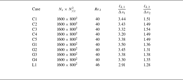


 Open access