


1. Introduction
Modal decomposition has become fundamentally important in turbulence research in terms of constructing a low-dimensional (low-order) representation in the Eulerian perspective and establishing an explicit connection of dynamic process between the physical and phase space (Holmes et al. Reference Holmes, Lumley, Berkooz and Rowley2012). Since Lumley (Reference Lumley1967, Reference Lumley1970) proposed the proper orthogonal decomposition (POD) in the realm of turbulence, a large variety of modal decomposition methods have been developed for more than 50 years. Coherent structures – organised fluid elements of significant lifetime and scale – can be extracted by these well-designed methods, enabling the mechanistic study of the essential dynamical features inherent in complex flows. Modal analysis has demonstrated its powerful roles in theoretical analysis and engineering applications (Taira et al. Reference Taira, Brunton, Dawson, Rowley, Colonius, McKeon, Schmidt, Gordeyev, Theofilis and Ukeiley2017, Reference Taira, Hemati, Brunton, Sun, Duraisamy, Bagheri, Dawson and Yeh2020), for example, shedding light on the potential mechanisms of the unsteadiness in shock wave/boundary layer interactions (Priebe et al. Reference Priebe, Tu, Rowley and Martín2016), self-similar behaviour in pipe flows (Hellström, Marusic & Smits Reference Hellström, Marusic and Smits2016) and providing insight into the dynamics of large-scale wavepackets in turbulent jets (Schmidt et al. Reference Schmidt, Towne, Rigas, Colonius and Brès2018), among others.
Some general consensus has been reached on the direction of the development of modal decomposition, even though various techniques are rooted in different physical considerations and mathematical operations. As suggested by Noack (Reference Noack2016), the first is to extend the information contained in the decomposed modes, i.e. improve the capability in characterizing desired evolutionary properties by adopting a more appropriate mathematical form for the modes. The second is to extract a sparse description of the dominant feature in the original high-dimensional dynamic system (Brunton, Proctor & Kutz Reference Brunton, Proctor and Kutz2016), which requires that we need to define what is called ‘dominant’ (maybe dynamically or in other senses) and determine how to extract these dominant components. Although increasingly sophisticated experimental techniques and high-performance computing have provided a huge mass of time-accurate flow field data, namely, a prerequisite to explore the transient and intermittent behaviours in statistically non-stationary flows, further development of modal-based time-frequency analysis is still highly desired (Schmidt, Colonius & Brès Reference Schmidt, Colonius and Brès2017; Nekkanti & Schmidt Reference Nekkanti and Schmidt2021). It is due to the fact that the conventional construction ideas of existing methods, such as time averaging and linear approximation, limit their ability to characterize the time-frequency information, which motivates us to introduce a new mathematical form of modal expansion to overcome this difficulty.
The two most popular modal analysis techniques, POD and dynamic mode decomposition (DMD; Schmid Reference Schmid2010), have demonstrated their good capabilities in a wide range of problems, though improvements are still to be raised for other special application scenarios. The core idea of POD is to find an orthonormal basis that spans a finite-dimensional subspace, such that the  $L^2$-norm of the projected data onto this subspace obtains its maximum in a time (or ensemble)-averaged sense (Holmes et al. Reference Holmes, Lumley, Berkooz and Rowley2012). This energy optimality makes it an efficient way to compress data, but the averaging process may result in the loss of key dynamical information. DMD is proposed to extract modes with temporal monochromaticity (spectral purity) through a linear approximation of the original nonlinear system, which can also be regarded as a finite-dimensional approximation of the Koopman operator (Rowley et al. Reference Rowley, Mezić, Bagheri, Schlatter and Henningson2009; Brunton et al. Reference Brunton, Budisić, Kaiser and Kutz2022). The eigenvalues and corresponding eigenvectors of the approximated system comprise the DMD modes, whose time coefficients are pure harmonics with exponential growth or decay. For mean-subtracted data, Chen, Tu & Rowley (Reference Chen, Tu and Rowley2012) have proved that DMD is equivalent to the discrete Fourier transform (DFT). Different from POD, DMD allows us to examine the spectral content of the system in a global manner. Nevertheless, the exponential oscillatory formulation ( ${\rm e}^{\lambda t}$) of the time coefficients limits its application to describe general nonlinear, non-stationary processes (e.g. processes with amplitude modulation or frequency modulation).
Recently, various time-frequency analysis strategies have been attempted by incorporating concepts in signal processing into the existing modal decomposition methods. Kutz, Fu & Brunton (Reference Kutz, Fu and Brunton2016) presented a recursive algorithm called multi-resolution DMD, in which the modes with the frequency characteristics localized in time are obtained by a removal-splitting operation. Another interesting attempt was made by Schmidt et al. (Reference Schmidt, Colonius and Brès2017), Towne & Liu (Reference Towne and Liu2019) and Nekkanti & Schmidt (Reference Nekkanti and Schmidt2021) based on the spectral proper orthogonal decomposition (SPOD; Towne, Schmidt & Colonius Reference Towne, Schmidt and Colonius2018). SPOD is a space–time formulation of POD, which inherits the basic idea of Lumley (Reference Lumley1967, Reference Lumley1970). For statistically stationary flows, it computes orthogonal modes that diagonalize the estimated cross-spectral density matrix at each frequency. As summarized by Nekkanti & Schmidt (Reference Nekkanti and Schmidt2021), two approaches have been presented to recover the time-frequency contents from the already computed SPOD modes: oblique projection in the time domain and convolution in the frequency domain. For other methods and examples, see Sieber, Paschereit & Oberleithner (Reference Sieber, Paschereit and Oberleithner2016), Mendez, Balabane & Buchlin (Reference Mendez, Balabane and Buchlin2019) and Mendez et al. (Reference Mendez, Ianiro, Noack and Brunton2023). These frameworks mentioned above can serve as a good pilot to guide the development of modal-based time-frequency analysis while further efforts are required to improve performance and operability.
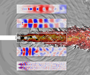
In this study, we will develop a novel data-driven modal analysis method referred to as reduced-order variational mode decomposition (RVMD), which is inspired by the Hilbert–Huang transform (HHT; Huang et al. Reference Huang, Shen, Long, Wu, Shih, Zheng, Yen, Tung and Liu1998) and a state-of-the-art signal-processing technique called variational mode decomposition (VMD; Dragomiretskiy & Zosso Reference Dragomiretskiy and Zosso2014). It is well known that HHT can provide a feasible path for dealing with nonlinear, non-stationary signals in the Hilbert view (Huang, Shen & Long Reference Huang, Shen and Long1999), which is different from the Fourier-based methods such as short-time Fourier transform and wavelet transform. HHT is implemented by decomposing the original time series into intrinsic mode functions (IMFs) using empirical mode decomposition (EMD), with each IMF reflecting a distinctive non-stationary property, and then applying Hilbert spectral analysis to obtain the time-varying envelopes and instantaneous frequencies. IMF represents a generalized Fourier expansion that can effectively characterize time-frequency contents with superior resolution (Huang et al. Reference Huang, Shen and Long1999). Drawing on the construction of VMD and combining the low-order representation, the proposed method can adaptively extract time-frequency features from space–time data; each RVMD mode can be regarded as an ‘elementary low-order dynamic process (ELD)’ which inherits the idea of IMF. Notably, the appealing features of RVMD are in line with the outlook of Noack (Reference Noack2016), as the direct result of a mathematically well-defined optimization problem. Two canonical flow problems, the transient cylinder wake and the planar supersonic jet, are employed to demonstrate the advantages of RVMD in revealing transient and non-stationary dynamics from complex fluid flows.
The remainder of this paper is organized as follows. Section 2 introduces some basic concepts, definitions and mathematical techniques in signal processing which constitute the cornerstone of RVMD. Section 3 formulates the proposed method, presents a specific algorithm and discusses the computational costs as well as the criteria for parameter setting. Section 4 elucidates the relations between RVMD and several existing methods, and presents a signal-processing analogous categorization of various modal techniques. In § 5, two cases are used to validate the capabilities and advantages of RVMD. Finally, concluding remarks are summarized in § 6.
2. Theoretical basis
As we know, the conventional framework of modal analysis is to seek a low-order representation of the space–time flow data  $q(\boldsymbol {x},t)$ written as
 \begin{equation} q(\boldsymbol{x},t)\simeq\sum_{k=1}^K \phi_k(\boldsymbol{x})c_k(t), \end{equation}
where  $\phi _k(\boldsymbol {x})$ is called the (spatial) mode and $c_k(t)$ is called the time-evolution coefficient; this pair is referred to as the $k$th mode. Specific determination of the modes, usually regarded as coherent structures, depends on the prior assumptions stemming from physical considerations. As shown by (2.1), each mode's spatial and temporal contents are separated, enabling us to study them in isolation. Particularly, as suggested by Schmid (Reference Schmid2010), the temporal dynamics (frequencies) contained in $c_k(t)$ are crucial for distinguishing the dynamic processes. Hence, to establish a modal decomposition method that can extract dynamic processes from statistically non-stationary flows, we start by considering the form of time-evolution coefficients. Since $c_k(t)$ is just a time series, examining the well-developed signal processing theory will help us to achieve that.
In the following, we first introduce the idea of time-frequency analysis for non-stationary signals, illustrating the concept of non-stationary models and their applicability to fluid dynamics (§ 2.1). Then we give the definition and properties of a specific model called intrinsic mode function (§ 2.1.1) and, based on this, determine the form of modes (namely, ELD) adopted in the present work (§ 2.1.2). Necessary mathematical definitions and manipulations are reviewed in § 2.2. We will convert the real-valued time-evolution coefficients to corresponding analytic signals (§ 2.2.1) and extend the idea of Wiener filtering (§ 2.2.2) to construct an optimization problem, leading to an adaptive filtering procedure that yields the modes.
2.1. Models for characterizing non-stationarity
For non-stationary signals/flows in which we are interested, the statistical properties vary with translation in time. Though an unbiased estimate of the time-varying statistics can be achieved by performing an ensemble average on a number of realizations (Bendat & Piersol Reference Bendat and Piersol2011), it is usually difficult (or expensive) to conduct such repeated experiments or simulations under statistically similar conditions. Therefore, we need techniques, usually referred to as the time-frequency analysis, that recover the non-stationarity from an individual record of the random processes/fields. Following Huang et al. (Reference Huang, Shen and Long1999), we consider a time-frequency representation of signals in the Hilbert view – each signal can be regarded as a combination of some elementary models, and each model reflects a distinctive non-stationary property that is easy to understand. Notably, this idea coincides with that in the modal analysis, dissecting a complex process into several representative elements. We will show later that the underlying similarity leads to a smooth and natural combination of the modal and signal-processing techniques.
As suggested by Bendat & Piersol (Reference Bendat and Piersol2011), three examples of such elementary non-stationary models include signals with: (1) time-varying mean value; (2) time-varying mean square value and (3) time-varying frequency structure. Interestingly, the underlying physical meanings of these three models are also concerned in fluid dynamics (turbulence) research as the first- and second-order statistics (mean and fluctuation) and the spectral contents (temporal dynamics). Here, we present the following situations to illustrate the capability of these models in characterizing non-stationary properties of fluid flows. For flow over an actively pitching/plunging airfoil, the mean flow is time-varying and deterministic, so the whole flow field should be described by the first model. One may also find this is consistent with the idea of triple decomposition suggested by Hussain & Reynolds (Reference Hussain and Reynolds1970). The intermittent behaviours common in various turbulent flows, as well as the amplitude modulation in wall turbulence (Hutchins & Marusic Reference Hutchins and Marusic2007; Mathis, Hutchins & Marusic Reference Mathis, Hutchins and Marusic2009), can be characterized by the second model. The frequency shifting in nonlinear wave evolution is a good example of the third model as discussed by Huang et al. (Reference Huang, Shen and Long1999). When a specific model has been adopted according to the physical situation and combined with some prior assumptions, the time-varying statistics can usually be estimated from a single record of non-stationary processes through a filtering operation; see Bendat & Piersol (Reference Bendat and Piersol2011) for examples in signal processing and Mathis et al. (Reference Mathis, Hutchins and Marusic2009) for an excellent example in wall turbulence.
2.1.1. Intrinsic mode function and narrow-band property
Intrinsic mode function (IMF), an ingenious non-stationary model which is much more general compared with the above three simple examples, was first proposed together with empirical mode decomposition by Huang et al. (Reference Huang, Shen, Long, Wu, Shih, Zheng, Yen, Tung and Liu1998). Nowadays, it has become the central concept of many modern time-frequency analysis techniques that have been widely applied, such as synchrosqueezed wavelet transform (Daubechies, Lu & Wu Reference Daubechies, Lu and Wu2011) and empirical wavelet transform (Gilles Reference Gilles2013). A specific definition of IMF suggested by Daubechies et al. (Reference Daubechies, Lu and Wu2011) is adopted in this work, which is slightly different from the original one and is more restrictive: IMF is a real-valued amplitude-modulated–frequency-modulated signal written as
 \begin{equation} c(t)=A(t)\cos\varphi(t), \end{equation}
with non-decreasing phase  $\varphi (t)$ and non-negative envelope $A(t)$. The envelope and the derivative of the phase $\mathrm {d}\varphi /\mathrm {d}t$ should vary much slower than the phase.
As seen, neither  $\varphi (t)$ nor $A(t)$ has an explicitly predefined form, reflecting the core idea of Huang et al. (Reference Huang, Shen, Long, Wu, Shih, Zheng, Yen, Tung and Liu1998): for a nonlinear and non-stationary signal, we should adapt the basis to data instead of adapt data to the basis. Thus, it is easy to find that all three aforementioned elementary non-stationary models and the Fourier/normal modes can be represented using IMFs. In addition, IMF always has a limited bandwidth, which means that each IMF oscillates around a specific frequency (referred to as ‘central frequency’ hereafter) with a narrow band due to the slow-varying $A(t)$ and $\mathrm {d}\varphi /\mathrm {d}t$ (see examples of Sharpley & Vatchev Reference Sharpley and Vatchev2006). Having been aware of the importance of the narrow-band property, Dragomiretskiy & Zosso (Reference Dragomiretskiy and Zosso2014) suggested a novel method called variational mode decomposition (VMD), which seeks modes while each being band-limited around the adaptively determined central frequency instead of explicitly using the formulation of IMF (2.2). This narrow-band prior makes VMD a fully non-recursive variational approach to extract scale-separated modes as components of a non-stationary signal, and becomes a core idea we have adopted in the present work.
2.1.2. Elementary low-order dynamic process (ELD)
Now, combining the idea of modal analysis discussed previously and the concept of IMF, we construct a space–time non-stationary model that can represent the dynamic processes in nonlinear, non-stationary flows. The ELD is proposed and defined as a space–time field which can be expressed in a low-order form,  $\phi (\boldsymbol {x})c(t)$, whose time-evolution coefficient $c(t)$ is an IMF. Since the spatial organization and temporal evolution of an ELD are separated, all the mathematical descriptions and the properties of $c(t)$ are directly inherited from IMF, and the narrow-band property is no exception. Hence, the ELD can also be considered to some extent as an extension of the ‘dynamic modes’ extracted by DMD (Schmid Reference Schmid2010), implying a basic understanding that the coherent structure usually evolves at a specific time scale. However, the ELD is tonal with a narrow bandwidth around a central frequency, while the dynamic mode evolves merely at a single frequency. Notably, the limitation in time-frequency representation of DMD and other modal techniques with spectral purity has already been noticed in recent studies on modal analysis (Sieber et al. Reference Sieber, Paschereit and Oberleithner2016; Mendez et al. Reference Mendez, Balabane and Buchlin2019). As suggested by Mendez et al. (Reference Mendez, Balabane and Buchlin2019), finite bandwidth rather than single frequency leads to time localization capabilities, which again supports our idea of constructing ELD.
Overall, after determining the form of modes – the ELD – we then seek a specific algorithm to extract these dominant elements from flow data. The extraction can be achieved through band-pass filtering using the narrow-band property, following the methodology proposed by Dragomiretskiy & Zosso (Reference Dragomiretskiy and Zosso2014).
2.2. Mathematical fundamentals
Before presenting the specific formulation of RVMD, we have to take a brief review of some definitions and manipulations in signal processing which provide us with the necessary mathematical tools. Consider a real-valued or complex-valued function  $c(t)$ (also referred to as a signal or time series); its Fourier transform (or spectrum) in a unitary form is
 \begin{equation} \hat{c}(\omega)=\mathcal{F}\{c(t)\}\equiv\frac{1}{\sqrt{2{\rm \pi}}} \int_{-\infty}^{\infty}c(t)\exp({-\mathrm{i}\omega t})\,\mathrm{d}t, \end{equation}
where  $\mathrm {i}=\sqrt {-1}$ is the imaginary unit. The two functions $|c(t)|^2$ and $|\hat {c}(\omega )|^2$, referred to as energy density and energy density spectrum, respectively, characterize the energy distributions over time and frequency. According to Parseval's theorem, we have
 \begin{equation} E\equiv\int_{-\infty}^{\infty}|c(t)|^2\,\mathrm{d}t= \int_{-\infty}^{\infty}|\hat{c}(\omega)|^2\,\mathrm{d}\omega, \end{equation}
with  $E$ denoting the total energy of the signal.
2.2.1. Analytic signal and instantaneous frequency
If we focus on a real-valued  $c(t)$ (since all the data in the real world are, naturally, real), which can be seen as an ‘oscillation’, a standard procedure that can obtain the information about the oscillation's amplitude and phase is to compute the analytic signal corresponding to $c(t)$ using a Hilbert transform (Cohen Reference Cohen1995). The Hilbert transform of a real-valued function $c(t)$ is a real-valued function defined by
 \begin{equation} \mathcal{H}\{c(t)\}\equiv c(t)*\frac{1}{{\rm \pi} t}=\frac{1}{\rm \pi}\mathrm{p.v.}\int_{-\infty}^{\infty} \frac{c(\tau)}{t-\tau}\mathrm{d}\tau, \end{equation}
where  $*$ denotes convolution and $\text {p.v.}$ denotes the principle value. Then, the analytic signal corresponding to (or the analytic representation of) real-valued $c(t)$ is defined as the following complex-valued function:
 \begin{equation} c_A(t)\equiv c(t)+\mathrm{i}\mathcal{H}\{c(t)\}.\end{equation}
An essential property of analytic signals is the unilateral spectrum
 \begin{equation} \hat{c}_A(\omega)=\left\{\begin{array}{@{}ll} 2\hat{c}(\omega) & \omega\geq0 \\ 0 & \omega<0 \end{array}\right..\end{equation}
Remarkably, the analytic representation does not alter the spectral contents of the original function as indicated by (2.7), and a recovery of  $c(t)$ can be easily made by taking the real part of $c_A(t)$ as indicated by (2.6). Another useful property of the analytic signal is that multiplying it with a pure exponential results in a simple frequency shifting
 \begin{equation} c_A(t)\exp({-\mathrm{i}\omega_0t})\stackrel{\mathcal{F}}{\longleftrightarrow} \hat{c}_A(\omega)*\delta(\omega+\omega_0)=\hat{c}_A(\omega+\omega_0), \end{equation}
where  $\delta ({\cdot })$ is the Dirac delta function. This formula stems from the basic modulation property of the Fourier transform.
We then explain why the analytic signal is important for the subsequent problem formulation by illustrating its physical meaning, and introduce a core concept of time-frequency analysis in the Hilbert view – the instantaneous frequency. Since the analytic signal is complex, it can be written in a polar form  $c_A(t)=A^*(t)\exp ({\mathrm {i}\varphi ^*(t)})$ with $A^*(t)\equiv |c_A(t)|$ and $\varphi ^*(t)\equiv \arg \{c_A(t)\}$. We have the following proposition: a complex-valued function $A^*(t)\exp ({\mathrm {i}\varphi ^*(t)})$ is analytic if the spectrum of $A^*(t)$ is contained in $(-\omega _0,\omega _0)$ and the spectrum of $\exp ({\mathrm {i}\varphi ^*(t)})$ is zero for $\omega \leq \omega _0$ (Cohen Reference Cohen1995). This is the key that makes analytic signals distinctive from general complex-valued functions – the spectral content of $A^*(t)$ is lower than the spectral content of $\exp {\mathrm {i}\varphi ^*(t)})$, so the latter can be regarded as a relatively high-frequency ‘oscillation’ while the former being the slow-varying amplitude of this oscillation, which coincides with the physical consideration when defining IMFs. In particular, for an IMF $c(t)=A(t)\cos \varphi (t)$ as defined in § 2.1.1, Bedrosian's theorem (Bedrosian Reference Bedrosian1963) implies that
 \begin{equation} c_A(t)=c(t)+\mathrm{i}\mathcal{H}\{c(t)\}=A(t)[\cos\varphi(t)+ \mathrm{i}\sin\varphi(t)]=A(t)\exp({\mathrm{i}\varphi(t)}). \end{equation}
Thus, the envelope and the phase of any IMF can be easily obtained by computing the modulus and argument of the corresponding analytic signal. Moreover, the ‘instantaneous frequency’ of  $c(t)$ is defined as the derivative of the oscillation phase $\mathrm {d}\varphi /\mathrm {d}t$, indicating how the spectral content varies with time. Examples and illustrations about the instantaneous frequency are provided by Huang et al. (Reference Huang, Shen and Long1999) and Cohen (Reference Cohen1995).
2.2.2. Wiener filtering
Recall the idea of this work mentioned in § 2.1 – extracting modes by filtering; we then show in practice how to construct an optimization problem that leads to frequency-domain filtering. Consider an observed signal  $f_0(t)$ consisting of the original signal $f(t)$ and a zero-mean (Gaussian) white noise $\eta$. The inverse problem of recovering the original signal from the observed data can be addressed by Tikhonov regularization, leading to a minimization problem
 \begin{equation} \min_f\left\{\|f-f_0\|^2+\alpha\|\partial_t f\|^2\right\}, \end{equation}
where  $\|{\cdot }\|$ denotes the $L^2$-norm and $\alpha$ is a positive regularization parameter. If the noise is Gaussian, then $\alpha$ can be optimally determined as the variance of the Gaussian noise; however, in VMD and the present work, $\alpha$ is determined empirically/posterior (Dragomiretskiy & Zosso Reference Dragomiretskiy and Zosso2014). The first term in the above formula is the square error and the second term is proportional to the square of root-mean-square bandwidth around a zero frequency as defined by Cohen (Reference Cohen1995). After being transformed into the frequency domain, this problem can be solved through a standard variational procedure, leading to a Wiener filtering on the observed data
 \begin{equation} \hat{f}(\omega)=\frac{1}{1+\alpha \omega^2}\hat{f}_0(\omega). \end{equation}
As shown, the recovered signal  $f$ is a low-pass narrow-band selection of the input $f_0$ around zero frequency. By using properties of analytic signals – shift the spectrum of the signal from a specific central frequency to zero such that the low-pass filter becomes a band-pass filter – Dragomiretskiy & Zosso (Reference Dragomiretskiy and Zosso2014) extends the classic Wiener filter into multiple and adaptive bands, namely VMD (see Appendix A). The proposed method inherits the idea of VMD, further combined with the non-stationary model (ELD) defined previously to deal with space–time flow data.
3. Reduced-order variational mode decomposition
3.1. Problem formulation
For flow data  $q(\boldsymbol {x},t)$ sampled from numerical simulations or experimental measurements, the proposed method seeks a group of triplets with a finite number $K$, written as
 \begin{equation} \left.\left\{\phi_k(\boldsymbol{x}),c_k(t),\omega_k\right\}\right|_{k=1}^K. \end{equation}
The spatial modes  $\phi _k(\boldsymbol {x}),\ \boldsymbol {x}\in \varOmega$ and time-evolution coefficients $c_k(t),\ t\in (-\infty,\infty )$ form a low-order approximation of $q(\boldsymbol {x},t)$, with $\varOmega$ denoting the spatial domain over which the flow is defined. In addition, $\omega _k$ is the central frequency, around which the time-evolution coefficient is band-limited (we will see later that $c_k(t)$ is computed by filtering around $\omega _k$). Note that the central frequency introduced here must be understood as an independent variable rather than a property of the time-evolution coefficient. All these functions are (locally) square-integrable due to the finite energy nature of the real fluid flows and can be further assumed to belong to a Hilbert space with inner product $\langle {\cdot },{\cdot }\rangle$ and induced norm $\|{\cdot }\|$. Following the formulation of POD (Holmes et al. Reference Holmes, Lumley, Berkooz and Rowley2012), specific definitions in space and time are
 $$\begin{gather} \|\phi(\boldsymbol{x})\|_{\boldsymbol{x}}\equiv\langle\phi,\phi\rangle^{1/2}_{\boldsymbol{x}}\quad \text{with}\ \left\langle \phi_1(\boldsymbol{x}),\phi_2(\boldsymbol{x})\right\rangle_{\boldsymbol{x}}= \int_\varOmega \phi_1(\boldsymbol{x})\overline{\phi_2(\boldsymbol{x})}\,\mathrm{d}\kern0.7pt \boldsymbol{x}, \end{gather}$$
 $$\begin{gather}\|c(t)\|_t\equiv\langle c,c\rangle^{1/2}_t\quad \text{with} \left\langle c_1(t),c_2(t)\right\rangle_t=\int_{-\infty}^\infty c_1(t)\overline{c_2(t)}\,\mathrm{d}t, \end{gather}$$
respectively. These definitions are applicable to both real-valued and complex-valued functions. Domains of  $\phi _k(\boldsymbol {x})$, $c_k(t)$ and $\omega _k$ are
 \begin{equation} \varPhi\equiv\left\{\phi(\boldsymbol{x})\in L^{2,\mathbb{R}}(\varOmega)\,|\, \|\phi(\boldsymbol{x})\|_{\boldsymbol{x}}=1\right\},\quad C\equiv L_{{loc}}^{2,\mathbb{R}}(-\infty,\infty),\quad \mathbb{R}^+, \end{equation}
respectively, where the subscript ‘ ${loc}$’ implies that the $L^2$-norm is finite on finite closed intervals in time. Remarkably, all these components are defined in the real domain, ensuring a straightforward flow field reconstruction and a clear physical meaning like that in POD. In addition, since the spatial modes are normalized, the energy of each mode is reflected by its time-evolution coefficient, i.e.
 \begin{equation} E_k=\left\|c_k(t)\right\|_t^2. \end{equation}
Additionally, the energy ratio can be further defined to measure the relative strength of each mode
 \begin{equation} \tilde{E}_k\equiv \frac{E_k}{\displaystyle\sum_{i=1}^K{E_i}}. \end{equation}
 The aim of RVMD is to adaptively seek  $K$ modes as described above to get a low-redundant approximation of the space–time data $q(\boldsymbol {x},t)$, with each mode being an ELD as defined in § 2.1.2. Here, the term ‘low-redundant’ is used to stress the following two aspects. First, when performing the RVMD, the number of modes (to quantify how sparse an approximate description is desired to characterize the data) is predetermined manually. This is different from the situation when using existing approaches (such as POD, DMD and SPOD), for which one computes a number of modes and then selects some representative, physically interpretable ones to aid the analysis of flow physics (Chen et al. Reference Chen, Tu and Rowley2012; Jovanović, Schmid & Nichols Reference Jovanović, Schmid and Nichols2014). In the RVMD, such a ‘selection’ is achieved simultaneously with the ‘computation’ procedure, and the sparsity (low-redundancy) is introduced at the very beginning. Second, since the temporal evolution of ELD is an amplitude-modulated–frequency-modulated signal (IMF) rather than a pure harmonic, the RVMD modes may represent dynamical behaviours in a more compact way. For example, a flow process with amplitude modulation can be represented by only one RVMD mode (see illustration in § 5.2). In contrast, for DMD/SPOD, one must combine several modes to recover such time-varying amplitude property (Schmidt et al. Reference Schmidt, Colonius and Brès2017; Towne & Liu Reference Towne and Liu2019; Nekkanti & Schmidt Reference Nekkanti and Schmidt2021).
In addition, since  $K$ is predetermined, it should be emphasized that RVMD does not guarantee a complete reconstruction of the flow field (especially the broadband stationary components induced by turbulence), which is different from existing methods such as POD and DFT. However, as stated by Holmes et al. (Reference Holmes, Lumley, Berkooz and Rowley2012) and Schmid (Reference Schmid2022): the most critical point of modal analysis is to extract and isolate the dominant dynamic behaviours, then get a better understanding of the fundamental mechanisms based on these modal results; accurately reproducing the data that have already been obtained is of secondary importance. Moreover, when constructing a low-dimensional model, one only needs to keep the dominant coherent structures (usually extracted by modal techniques) and simulate or model the less energetic, apparently incoherent turbulent background (Lumley & Yaglom Reference Lumley and Yaglom2001; Holmes et al. Reference Holmes, Lumley, Berkooz and Rowley2012). Hence, this ‘limitation’ does not compromise the applicability of RVMD.
The goal is achieved by limiting the time-evolution coefficients to have a compact bandwidth rather than explicitly using the formulation of IMF. Similar to the filtering procedure shown in § 2.2.2, the RVMD modes are computed by minimizing the following two components: the measure of the deviation between the original field and the mode-reconstructed one, and the sum of the bandwidths of the coefficients. Following the formulation of VMD and the theoretical basis discussed previously, the resulting unconstrained optimization problem is given by
 \begin{align} & \min_{\left.\left\{\phi_k(\boldsymbol{x}),c_k(t),\omega_k\right\}\right|_{k=1}^K} \left\{\alpha\sum_{k=1}^K\left\|\partial_t\left\{\left[\left(\delta(t)+\mathrm{i} \frac{1}{{\rm \pi} t}\right)*c_k(t)\right]\exp({-\mathrm{i}\omega_k t})\right\}\right\|_t^2 \vphantom{\left\|q(\boldsymbol{x},t)-\sum_{k=1}^K\phi_k(\boldsymbol{x})c_k(t)\right\|_\mathrm{F}^2}\right.\nonumber\\ &\quad \left.+\left\|q(\boldsymbol{x},t)-\sum_{k=1}^K\phi_k(\boldsymbol{x})c_k(t)\right\|_\mathrm{F}^2\right\}. \end{align}
The convolution of  $\delta (t)+\mathrm {i}/{\rm \pi} t$ and $c_k(t)$ leads to the analytic representation of $c_k(t)$, then an exponential with frequency $\omega _k$ is multiplied to shift the mode's spectrum to the baseband. The norm $\|{\cdot }\|_\mathrm {F}$ for a space–time function $f(\boldsymbol {x},t)$ in $L^{2,\mathbb {R}}(\varOmega )\times L_{loc}^{2,\mathbb {R}}(-\infty,\infty )$ is defined as
 \begin{equation} \|f(\boldsymbol{x},t)\|_\mathrm{F}^2\equiv\int_\varOmega\int_{-\infty}^\infty f(\boldsymbol{x},t)\overline{f(\boldsymbol{x},t)}\,\mathrm{d}t\,\mathrm{d}\boldsymbol{x}, \end{equation}
which corresponds to the Frobenius norm of matrices. The regularization parameter  $\alpha$, referred to as the filtering parameter hereafter, reflects the relative importance of compact bandwidth and better reconstruction. Both $\alpha$ and $K$ should be input in advance.
For mathematical simplicity, a frequency-domain alternative of (3.7) is used to compute the RVMD modes. The detailed derivation is shown in Appendix B and, finally, we get the following optimization problem:
 \begin{align} & \min_{\left.\left\{\phi_k(\boldsymbol{x}),\hat{c}_k(\omega),\omega_k\right\}\right|_{k=1}^K} \left\{\sum_{k=1}^K\int_{0}^\infty 2\alpha (\omega-\omega_k)^2 |\hat{c}_k(\omega)|^2\,\mathrm{d}\omega \vphantom{\left\|q(\boldsymbol{x},t)-\sum_{k=1}^K\phi_k(\boldsymbol{x})c_k(t)\right\|_\mathrm{F}^2}\right.\nonumber\\ &\quad \left.+\int_\varOmega\int_{0}^\infty\left|\hat{q}(\boldsymbol{x},\omega)-\sum_{k=1}^K \phi_k(\boldsymbol{x})\hat{c}_k(\omega)\right|^2\mathrm{d}\omega\,\mathrm{d}\boldsymbol{x}\right\}. \end{align}
As shown, the first term is proportional to the square of root-mean-square bandwidth (Cohen Reference Cohen1995) of the time-evolution coefficient around the corresponding central frequency. It can be understood as the second-order moment of  $\omega$ about $\omega _k$ with the energy density spectrum of $c_k(t)$ as the weight. By minimizing this bandwidth term, the spectrum of each mode will be compact around $\omega _k$, which again explains why we term $\omega _k$ the central frequency. The objective function is to be optimized over all the three components in their feasible regions:
 \begin{align} \phi_k(\boldsymbol{x})\in\varPhi,\quad \hat{c}_k(\omega)\in\hat{C}\equiv \left\{\hat{c}(\omega)\in L_{{loc}}^{2,\mathbb{C}}(-\infty,\infty)\,|\, \hat{c}(-\omega)=\overline{\hat{c}(\omega)}\right\},\quad \omega_k\in\mathbb{R}^+. \end{align}
Particularly, the so-called adaptivity is achieved by optimizing over the central frequencies, thanks to the mathematical properties of analytic signals that enable us to construct band-pass filtering easily. Furthermore, the spatial modes  $\phi _k(\boldsymbol {x})$ are not restricted to be mutually orthogonal. That is, RVMD inherits the advantages of DMD that the non-orthogonal modes provide the ability to capture the essential dynamical behaviours in systems with non-normal dynamical generators (Trefethen et al. Reference Trefethen, Trefethen, Reddy and Driscoll1993; Schmid Reference Schmid2007; Jovanović et al. Reference Jovanović, Schmid and Nichols2014).
The intended use of RVMD is to discover the (hidden) nonlinear, non-stationary dynamics expressed in a low-order form (the ELDs), which usually act as some ‘tonal’ components of fluid flows. Since scale separation is achieved through this decomposition, each mode is expected to reflect a distinctive evolutionary characteristic, improving our ability to understand the dominant, coherent features in complex flows. Moreover, the definition of ELD enables us to directly apply the well-established non-stationary signal processing techniques to the RVMD results, forming a novel modal-based, quantitative time-frequency analysis framework for fluid dynamics.
In addition, the scope of application may include: (1) the flow with a transition from one state to another, in which transient dynamics localized in time and frequency exist and (2) the flow with tonal components surrounded by broadband stationary noise induced by turbulence. Since IMFs are amplitude-modulated–frequency-modulated signals which remind us of the treatment in Landau's theory of nonlinear stability analysis (Drazin & Reid Reference Drazin and Reid2004; Landau & Lifshitz Reference Landau and Lifshitz2013), they are very suited for representing transient dynamical evolutions (see § 5.1 for example). For the second type of problem, it should be clarified that the tonal components in turbulent flows may not be non-stationary. However, suppose someone believes that all the tonal components in turbulent flows are stationary or approximately linear and, thus, characterize and model the dynamics using Fourier modes or normal modes without careful verification. In this case, they will possibly miss some non-trivial properties of the actual nonlinear evolutions, propose a failed modelling and lose the underlying physical mechanisms (see § 5.2 for example). Overall, we believe that RVMD, together with the related analysis framework in the Hilbert view, can become a useful tool complementary to the classic methods such as the POD, DMD and SPOD, which are commonly not suited for treating fluid flows especially featured by a transient or non-stationary nature.
3.2. Computing the RVMD modes
After establishing the optimization problem (3.9), we provide a viable path to solve it iteratively using the block coordinate descent algorithm (see Liu et al. Reference Liu, Hu, Li and Wen2020). Each component in each mode is successively updated (from  $k=1$ to $K$, from $\phi _k$, $\hat {c}_k$ to $\omega _k$) in one iteration according to the following equations:
 $$\begin{gather} \phi_k^{n+1}(\boldsymbol{x})=\frac{\displaystyle\mbox{Re}\left\{\int_{0}^\infty \overline{\hat{c}_k^n(\omega)}\hat{r}^n_k(\boldsymbol{x},\omega)\,\mathrm{d}\omega\right\}}{\displaystyle\left\|\mbox{Re} \left\{\int_{0}^\infty\overline{\hat{c}_k^n(\omega)}\hat{r}^n_k (\boldsymbol{x},\omega)\,\mathrm{d}\omega\right\}\right\|_{\boldsymbol{x}}}, \end{gather}$$
 $$\begin{gather}\hat{c}_k^{n+1}(\omega)=\hat{g}_k^n(\omega)\int_\varOmega \phi_k^{n+1}(\boldsymbol{x})\hat{r}^n_k(\boldsymbol{x},\omega)\,\mathrm{d}\boldsymbol{x},\quad (\omega\geq0) \end{gather}$$
 $$\begin{gather}\omega_k^{n+1}=\frac{\displaystyle\int_0^\infty\omega\left|\hat{c}_k^{n+1}(\omega)\right|^2 \mathrm{d}\omega}{\displaystyle\int_0^\infty\left|\hat{c}_k^{n+1}(\omega)\right|^2\mathrm{d}\omega}. \end{gather}$$
In these formulae, the filtering function for the  $k$th mode at iteration step $n$ is defined as
 \begin{equation} \hat{g}_k^n(\omega)\equiv1/[1+2\alpha(\omega-\omega_k^n)^2],\quad(\omega\geq0) \end{equation}
and the residual function  $\hat {r}^n_k(\boldsymbol {x},\omega )$ for the $k$th mode at iteration step $n$ is defined as the remaining portion of the original data after excluding other modes
 \begin{equation} \hat{r}^n_k(\boldsymbol{x},\omega)\equiv\hat{q}(\boldsymbol{x},\omega)-\sum_{i=1}^{k-1} \phi_i^{n+1}(\boldsymbol{x})\hat{c}_i^{n+1}(\omega)-\sum_{i=k+1}^{K}\phi_{i}^{n} (\boldsymbol{x})\hat{c}_i^{n}(\omega). \end{equation}
The meaning of each formula is straightforward. The spatial mode is updated as the normalized, real part of the frequency-domain inner product of residual function and coefficient. The time-evolution coefficient is updated as the space-domain inner product of the residual function and spatial mode, and then filtered by  $\hat {g}_k^n$. Next, the central frequency is updated as the average value of the frequency weighted by the energy density spectrum of $c_k(t)$, which coincides with the definition of ‘average frequency’ by Cohen (Reference Cohen1995). That is, though the central frequency is not defined as the property of $c_k(t)$, the resulting value of $\omega _k$ does reflect the intrinsic spectral property of the resulting $c_k(t)$. Remarkably, all these manipulations are not constructed artificially as in some recursive modal decomposition methods, but are the direct result of solving the optimization problem (see Appendix C for the detailed derivation).
Some technical issues about the solving procedure are clarified below. First, since the problem at hand is a highly nonlinear, multivariate optimization, the proposed algorithm does not guarantee to converge to the unique global minimum theoretically, and the results (the local minimum), indeed, depend on parameters and initialization to some extent. Discussion on the parameter setting can be found in § 3.4, and a series of tests are included in § 5.2.2 to illustrate the parameter dependence practically. Second, the solving procedure is operated over the positive half of the frequency domain, and the time-evolution coefficient  $c_k(t)$ can be reconstructed directly at the end using the Hermitian symmetry. Third, though the data have been defined in the infinite time domain, we actually deal with a short-time discrete sample. Therefore, the sample should be implicitly considered as a one-period extraction from infinite, periodic data. Based on this point, one may find that the energy ratio of a transient mode (which is finite in time) would decrease linearly versus the window size. In practice, as demonstrated by the example of transient cylinder wake (see § 5.1), the transient process can be captured by RVMD, providing the window size is not extremely long with respect to the characteristic time scale of this process. More importantly, the proposed method is capable of resolving the instantaneous mode energy (envelope), which is independent of the window size and thus reliably facilitates our understanding of these transient dynamics. Fourth, the Gibbs phenomenon arises due to the discontinuity at the signal boundaries, also referred to as the ‘end effects’ in IMF extraction and Hilbert transform (Huang et al. Reference Huang, Shen, Long, Wu, Shih, Zheng, Yen, Tung and Liu1998). Although we can not eliminate this effect, several remedies exist. A simple, commonly used pre-processing technique that can considerably (but not completely) suppress the end effects, mirror extension, is adopted in the present work. Prior to the computation, the sampled data are extended by half its length at each side, and the extended part is mirror-symmetrical with the original data about each end. When the coefficient $c_k(t)$ has been reconstructed from its spectrum, the extended part at both ends is discarded to get the final result.
The complete algorithm in matrix form for computing the RVMD modes is outlined as follows. After performing the mirror extension, the flow field snapshots are collected as the data matrix
 \begin{equation} \boldsymbol{\mathsf{Q}}\in\mathbb{R}^{S\times T}, \end{equation}
where  $S$ and $T$ denote the numbers of sampling points in space and time, respectively. The RVMD modes are represented as column vectors
 \begin{equation} \boldsymbol{\phi}_k\in\mathbb{R}^{S},\quad \boldsymbol{c}_k\in\mathbb{R}^{T}. \end{equation}
We then use superscript  $({\cdot })^\mathrm {T}$ to denote the transpose, $({\cdot })^*$ to denote the conjugate, and $({\cdot })^\mathrm {H}$ to denote the conjugate transpose of matrices and vectors. Another two diagonal matrices are further defined: the non-negative frequency matrix $\boldsymbol{\mathsf{W}}=\mathrm {diag}(\boldsymbol {\omega })$ with elements $\omega _i=if_s/T, i=0,1,2,\ldots,T/2$, where $f_s$ is the sampling frequency; and the filtering matrix $\hat {\boldsymbol{\mathsf{G}}}_k^n=\mathrm {diag}(\boldsymbol {\hat {g}}^n_k)$ with elements $\hat {g}_{k,i}^n=1/[{1+2\alpha (\omega _i-\omega _k^n)^2}],\ i=0,1,2,\ldots,T/2$.
Algorithm (Reduced-order variational mode decomposition, RVMD)
(1) Initialize $\{\boldsymbol {\phi }_k,\boldsymbol {\hat {c}}_k,\omega _k\}|_{k=1}^K$ and set iteration step $n\leftarrow 0$.
(2) Loop:
Set
$n\leftarrow n+1$, for $k=1$ to $K$ do:(a) update the residual matrix for the
$k$th mode using
(3.18)\begin{equation} \hat{\boldsymbol{\mathsf{R}}}_k^n=\hat{\boldsymbol{\mathsf{Q}}} -\sum_{i=1}^{k-1}\boldsymbol{\phi}_i^{n+1}\boldsymbol{\hat{c}}_i^{n+1,\mathrm{T}} -\sum_{i=k+1}^K\boldsymbol{\phi}_i^{n}\boldsymbol{\hat{c}}_i^{n,\mathrm{T}}; \end{equation}(b) update the spatial mode using
(3.19)\begin{equation} \boldsymbol{\phi}_k^{n+1}=\frac{\mbox{Re}\left\{\hat{\boldsymbol{\mathsf{R}}}^{n}_k\boldsymbol{\hat{c}}_k^{n,*}\right\}}{\left\| \mbox{Re}\left\{\hat{\boldsymbol{\mathsf{R}}}^{n}_k\boldsymbol{\hat{c}}_k^{n,*}\right\}\right\|}; \end{equation}(c) update the Fourier transform of the time-evolution coefficient using
(3.20)\begin{equation} \boldsymbol{\hat{c}}_k^{n+1}=\hat{\boldsymbol{\mathsf{G}}}_k^n\hat{\boldsymbol{\mathsf{R}}}^{n,\mathrm{T}}_k \boldsymbol{\phi}_k^{n+1}; \end{equation}(d) update the central frequency using
(3.21)\begin{equation} \omega_k^{n+1}=\frac{\boldsymbol{\hat{c}}_k^{n+1,\mathrm{H}}\boldsymbol{\mathsf{W}} \boldsymbol{\hat{c}}_k^{n+1}}{\boldsymbol{\hat{c}}_k^{n+1,\mathrm{H}}\boldsymbol{\hat{c}}_k^{n+1}}. \end{equation}
Until convergence:
(3.22)i.e. the iteration difference (the left-hand side) is less than a given tolerance\begin{equation} \sum_{k=1}^K\frac{\|\boldsymbol{\hat{u}}_k^{n+1}-\boldsymbol{\hat{u}}_k^n \|_\mathrm{F}}{\|\boldsymbol{\hat{u}}_k^n\|_\mathrm{F}}<\epsilon,\quad \text{with}\ \boldsymbol{\hat{u}}_k^n\equiv\boldsymbol{\phi}_k^n\boldsymbol{\hat{c}}_k^{n,\mathrm{T}}, \end{equation}$\epsilon$.(3) Reconstruct the time-evolution coefficient
$\boldsymbol {c}_k$ from $\boldsymbol {\hat {c}}_k$ using the Hermitian symmetry and inverse Fourier transform to obtain the RVMD modes $\{\boldsymbol {\phi }_k,\boldsymbol {c}_k,\omega _k\}|_{k=1}^K$.


A specific implementation of RVMD is available at https://github.com/ZimoLiao/rvmd.
3.3. Assessment of computational cost
The proposed large-scale multivariate optimization is solved iteratively and, therefore, may take much longer time than that in traditional modal decomposition methods such as POD and DMD. This is natural since the proposed method pursues something non-trivial – adaptive extraction of nonlinear, non-stationary dynamics – instead of the properties inherent in linear algebra or linear dynamical systems (e.g. eigenvalues and eigenmodes). Here we present a quantitative assessment of the computational cost of the proposed algorithm. Particularly, considering the fact that the actual computation time depends on both software and hardware, we focus on a more general problem – how the cost scale with the problem size.
In the following, the computation time scaling of the RVMD method is estimated based on extensive tests of the data matrix sampled from the first example problem (the transient cylinder wake). Specifically, we performed 120 tests to compute the RVMD modes by choosing the number of modes  $K=5,10,15,20$, based on various sample sizes with the number of spatial sampling points $S=512,1024,2048,4096,8192,16\,384$ and the number of snapshots $T=32,64,128,256,512$. For each test, the ‘computation time per step’ is obtained as an average of the 500-step iterating time of the RVMD optimization. All the results are obtained by single-core computing using an open-source C++ library Eigen on an AMD EPYC 7282 16-core processor. Finally, an empirical scaling relation is fitted between the cost and the sample sizes.
Figure 1 shows the computation time per step for different numbers of modes  $K$. Each red line represents a group of tests at the same $(S,T)$, and the results are normalized by the value at $K=5$. The results obtained indicate that the computation time per step is approximately linearly related to $K$, which is in line with our expectation since each ( $k$th) RVMD mode is computed identically in the proposed algorithm. Consequently, we then concentrate on the relationships between the computation time per mode per step (averaged for different $K$) and the spatial/temporal size $(S,T)$; the results are fitted in log-log coordinates (see figure 2). Accordingly, a simple, fully empirical scaling relation can be approximated as
 \begin{equation} \text{computation time per step}\sim KS^{1.1}T^{1.1}. \end{equation}
In addition, the total time of computing all the RVMD modes is proportional to the number of iteration steps. It should be noted that the number of iteration steps depends strongly on the parameters (tolerance  $\epsilon$ and filtering parameter $\alpha$), the initialization and the flow data themselves. Here, the computation times and related parameters for the two cases in § 5 are listed in table 1, providing a quantitative, practical acquaintance with the computational cost of the proposed algorithm. Notably, since the updates in the proposed algorithm are all matrix calculations, it could be accelerated using some well-developed parallel linear algebra libraries.
Computation time scale with  $K$.
$K$.

Computation time scale with  $S$ and $T$.
$T$.

Computational cost for the two examples.

3.4. Criteria for parameter setting
As stated, there are two input parameters, the number of modes  $K$ and the filtering parameter $\alpha$, on which the RVMD results depend. In addition, the initialization of central frequencies also affects what ELDs the RVMD will find. Here we discuss the parameter dependence theoretically and provide some criteria/recommendations for determining these quantities. A detailed parametric study can be found in § 5.2, practically demonstrating the following discussions and showing how a posterior selection of the parameters is achieved.
First, consider the most critical input of RVMD – the filtering parameter  $\alpha$, which determines the shape of the filter and further affects the tradeoff between accurate reconstruction and limited bandwidth. According to (3.14), the bandwidth $\varDelta$ for the filtering function can be derived from $\alpha$
 \begin{equation} \varDelta=\sqrt{(2\sqrt{2}-2)/\alpha}. \end{equation}
This is the frequency interval between the filter's two half-power points (cutoff frequencies), following the standard definition of the bandwidth of a band-pass filter (different from the abovementioned root-mean-square bandwidth of a signal). Figure 3 depicts filtering functions with different  $\alpha$ and central frequencies $\omega _k$, providing an illustration of the above statements. Two criteria that restrict the upper and lower bound of the filter bandwidth (and, hence, the filtering parameter $\alpha$) are: (1) $\varDelta$ should be greater than the frequency resolution of the observed snapshots since we actually handle discrete samples. Otherwise, the resulting RVMD time-evolution coefficients approach pure harmonics and thus can not characterize non-stationary properties; (2) $\varDelta$ should be small enough to distinguish different tonal dynamics in the considered flow. If $\varDelta$ is too large, e.g. spans the whole frequency domain, the time-evolution coefficients may contain multiple characteristic frequencies like that in POD and reflect no insight into distinctive dynamics.
The filtering functions in RVMD with different filtering parameter  $\alpha$ and central frequencies $\omega _k$. The bandwidths of the filters are indicated using a light-red background.

Second, the setting of  $K$ is relatively arbitrary. The number of modes does not alter the adaptivity of RVMD or the dynamic properties of the resulting modes, so this parameter is merely the expected number of the ELDs contained in the specific fluid flow. Notably, it is challenging to accurately predetermine the number of ELDs in a complex flow problem. As shown by VMD, for too large or too small $K$, one may get over-decomposing or under-decomposing results, which may depart from our expectation – scale separation, low-redundancy and physical interpretability. It is no different from the shortcomings of classic segmentation or characteristic extraction techniques. However, in both situations, when over- or under-decomposing, VMD and the proposed RVMD produce predictable results, and a posterior adjustment on $K$ can be made. Finding a criterion for the automatic determination of the number of modes (the low-order dynamics) is a significant and difficult problem that is beyond the scope of this work.
Third, since the block coordinate descent algorithm cannot guarantee to find the global minimum for the constructed optimization problem, different central frequencies initialization strategies may lead to different local minima, i.e. the RVMD modes. When we know very little about the frequency characteristics of the flow, initializing the central frequencies to be uniformly distributed over the entire frequency domain is recommended. In this situation, no prior knowledge or assumption is required. Furthermore, when a qualitative or quantitative understanding of the frequency characteristics has been established, e.g. through the PSD of the probed signals or the prediction based on theoretical analysis, a user-defined central frequencies initialization may lead to better performance – faster convergence and a smaller number of modes that is enough to capture the dominant dynamics – of the proposed algorithm.
4. Relation to existing methods
This section expounds on the relations between RVMD and some classic modal decomposition methods. We show that the proposed method can be converted into POD when the filtering parameter equals zero; similarities and differences between RVMD and some recently presented methods are also discussed. In addition, we present a signal-processing analogous categorization of existing modal decomposition methods based on their abilities in time-frequency representation.
4.1. Proper orthogonal decomposition
As the filtering parameter  $\alpha$ is set as zero, the bandwidth term in (3.7) vanishes and the optimization problem turns into
 \begin{equation} \left.\begin{gathered} \min_{\left\{\phi_k(\boldsymbol{x}),c_k(t)\right\}} \left\{\left\|q(\boldsymbol{x},t)-\sum_{k=1}^K\phi_k(\boldsymbol{x})c_k(t)\right\|_{F}^2\right\}, \\ \text{s.t.}\quad \|\phi_k(\boldsymbol{x})\|_{\boldsymbol{x}}=1,\quad k=1,2,\ldots,K. \end{gathered}\right\} \end{equation}
Here the normalization constraint on  $\phi _k$ is explicitly written. This problem can be converted to the following minimization over the spatial modes:
 \begin{equation} \left.\begin{gathered} \min_{\left\{\phi_k(\boldsymbol{x})\right\}} \left\{\left\|q(\boldsymbol{x},t)-\sum_{k=1}^K \frac{\langle\phi_k(\boldsymbol{x}),q(\boldsymbol{x},t) \rangle_{\boldsymbol{x}}}{\|\phi_k(\boldsymbol{x})\|_{\boldsymbol{x}}^2} \phi_k(\boldsymbol{x})\right\|_{F}^2 \right\}, \\ \text{s.t.}\quad\|\phi_k(\boldsymbol{x})\|_{\boldsymbol{x}}=1,\quad k=1,2,\ldots,K. \end{gathered}\right\} \end{equation}
For discrete data, the Frobenius norm is equivalent to a (spatial)  $L^2$-norm combined with a summation over time (time average multiplied by a constant), so the optimization problem (4.2) is exactly what POD solves (Holmes et al. Reference Holmes, Lumley, Berkooz and Rowley2012). Since both RVMD and POD are based on a similar optimization framework and the modes are defined in the real domain, the interpretation of the modes (spatial function and the temporal coefficients) and the flow field reconstruction procedure in RVMD are the same as that in POD.
4.2. Sieber's method and multiscale POD
As stated, based on the discussion about non-stationary models and the narrow-band property of ELDs, we adopt a filtering procedure to extract and isolate coherent structures. The concept of ‘extracting by filtering/scale separating’ is not unfounded in the realm of fluid dynamics: originated from the Fourier analysis, progressed by the well-known dynamic mode decomposition (Schmid Reference Schmid2010), and recently extended and generalized by Sieber et al. (Reference Sieber, Paschereit and Oberleithner2016) and Mendez et al. (Reference Mendez, Balabane and Buchlin2019). The method of Sieber et al. (Reference Sieber, Paschereit and Oberleithner2016) is referred to as the so-called Sieber's SPOD hereafter, following the statements of Mendez et al. (Reference Mendez, Balabane and Buchlin2019), to distinguish it from another popular method named SPOD (Towne et al. Reference Towne, Schmidt and Colonius2018).
Since the eigenbasis of a Toeplitz circulant matrix is a Fourier basis (Grenander & Szegö Reference Grenander and Szegö1958), Sieber achieves a direct interpolation between the POD and DFT by performing a diagonal low-pass filtering on the temporal correlation matrix  $\boldsymbol{\mathsf{K}}$. The temporal coefficients $\boldsymbol {c}_k$ of Sieber's SPOD are computed as the eigenvectors of the filtered matrix
 \begin{equation} \boldsymbol{\mathsf{S}}\boldsymbol{c}_k=\lambda_k\boldsymbol{c}_k\quad\text{with}\ S_{i,j}=\sum_{k=-N_f}^{N_f}g_k K_{i+k,j+k}, \end{equation}
where  $g_k$ is a symmetric finite impulse response filter with length $2N_f+1$; the spatial modes are obtained by projecting the snapshots onto the temporal coefficients. The multiscale POD (mPOD) proposed by Mendez et al. (Reference Mendez, Balabane and Buchlin2019) takes the idea of Sieber's method – computing coefficients through the temporal correlation matrix – a step further by introducing the multi-resolution analysis (MRA) from wavelet theory. First, the temporal correlation matrix is split into the contributions of different scales using MRA; second, the optimal basis is extracted from each scale using POD. Since both methods implicitly include the ‘narrow-band’ prior, they can (for proper filtering or splitting) produce temporal coefficients that resemble the IMFs. Therefore, the instantaneous frequencies of the mode coefficients can be computed for analysis (Lückoff et al. Reference Lückoff, Sieber, Paschereit and Oberleithner2019) as we do in the present work.
As a comparison, the filtering procedure in RVMD can be written as
 $$\begin{gather} \hat{c}_k(\omega)=\beta_k \hat{g}_k(\omega)\int_{-\infty}^{\infty}\left[\int_\varOmega\overline{\hat{r}_k(\boldsymbol{x},\omega')} \hat{r}_k(\boldsymbol{x},\omega)\,\mathrm{d}\boldsymbol{x}\right]\hat{c}_k(\omega')\,\mathrm{d}\omega', \end{gather}$$
 $$\begin{gather}c_k(t)=\beta_k g_k(t)*\int_{-\infty}^{\infty}\left[\int_\varOmega r_k(\boldsymbol{x},t)r_k(\boldsymbol{x},t')\,\mathrm{d}\boldsymbol{x}\right] c_k(t')\,\mathrm{d}t', \end{gather}$$
in the frequency domain and time domain, respectively. For the  $k$th RVMD mode, $\beta _k$ is a constant that contributes to the magnitude of $c_k(t)$; $\mathcal {F}\{g_k(t)\}=\hat {g}_k(\omega )\equiv 1/[1+2\alpha (|\omega |-\omega _k)^2]$ is the filtering function with an even extension (defined in the whole frequency domain). Here, we assume that the iterative optimization has reached convergence (at least, in a numerical sense) and denote $\hat {c}_k\equiv \hat {c}_k^{n+1}\approx \hat {c}_k^n$, so do other components. The derivations are shown in Appendix D. Though the basic ideas of RVMD and the above two methods exhibit similarities, the differences in the mathematical manipulation can immediately be found by comparing (4.4), (4.5) and (4.3). In RVMD, the filter acts on the time-evolution coefficient, so the filtering parameter $\alpha$ directly controls the spectral property of the extracted low-order modes and the physical meaning is straightforward; while in Sieber's SPOD and mPOD, the filter acts on the temporal correlation through a matrix convolution, complicating its relation to the mode coefficients.
4.3. A signal-processing analogous categorization
According to the ability to describe temporal evolution, the existing modal techniques can be generally divided into three categories: time-domain, frequency-domain and time-frequency methods. First, since POD does not isolate the dynamics, it should be regarded as a fully time-domain method. Second, while both DMD and SPOD modes oscillate at a single frequency, they can be categorized as frequency-domain methods. Third, according to Huang et al. (Reference Huang, Shen and Long1999), the time-frequency methods can be further divided into two classes: the Fourier view and the Hilbert view. As mentioned previously, short-time Fourier transform and wavelet transform are the two popular Fourier-based frameworks for carrying out time-frequency analysis. The multi-resolution DMD (Kutz et al. Reference Kutz, Fu and Brunton2016) lies in this hierarchy, which adopts wavelet-based multiscale analysis, splitting the time-frequency domain into multiple sub-domains in advance to perform DMD. The proposed RVMD belongs to the time-frequency methods in the Hilbert view, obviously. Although Sieber's SPOD and mPOD produce modes with coefficients resembling the IMFs, both works did not identify or establish the underlying connection between modal analysis and non-stationary signal processing. In this paper, the concept of ELD is defined explicitly based on an in-depth understanding of non-stationary signal processing in the Hilbert view; and the corresponding time-frequency analysis framework is smoothly and naturally introduced into the realm of fluid dynamics research in a well-defined way.
5. Applications
In this section, we apply RVMD to two examples of canonical flow problems: the transient cylinder wake and the planar supersonic jet, and both are contained in the scope of application as stated in § 3.1. The first example is intended to introduce the modal-based time-frequency analysis framework in the Hilbert view, and the second example is included to demonstrate the applicability of RVMD to turbulent flows in terms of extracting tonal dynamics with hidden nonlinear, non-stationary properties. The parameter dependence of RVMD is also studied in the latter case to verify our statements in § 3.4.
5.1. The transient cylinder wake
5.1.1. Flow configuration
We begin with considering the transient cylinder wake, a widely adopted problem to illustrate and validate low-dimensional modelling (Noack et al. Reference Noack, Afanasiev, Morzyński, Tadmor and Thiele2003; Brunton et al. Reference Brunton, Proctor and Kutz2016). A two-dimensional incompressible flow past a cylinder is simulated using a lattice Boltzmann solver; the flow is initially set as an unstable steady state and then gradually evolves to a periodic vortex shedding – known as the von Kármán vortex street. The flow variables are non-dimensionalized by the cylinder diameter  $D$, the uniform inflow velocity $U$ and the kinematic viscosity $\nu$. We set the Reynolds number $Re\equiv UD/\nu$ equal to $100$ to ensure the onset of vortex shedding (Zebib Reference Zebib1987), similar to the numerical set-ups of Noack et al. (Reference Noack, Stankiewicz, Morzynski and Schmid2016). The origin of coordinates coincides with the centre of the cylinder, and the computational domain is set as $(x,y)\in [-10,15]\times [-10,10]$. A uniform inflow condition $u=1,v=0$ is implemented at the inlet and transverse boundaries, and an extrapolation condition at the outlet boundary. The no-slip boundary condition at the cylinder is imposed by the immersed boundary method.
To include the whole transient process and ensure a time resolution high enough,  $600$ snapshots of the mean-subtracted velocity fields $(u,v)$ with sampling interval $\varDelta tU/D=0.25=1/\tilde {f}_s$ (with $\tilde {f}_s$ denoting the dimensionless sampling frequency) are collected to perform RVMD. In this case, we set the number of modes $K=10$ and the filtering parameter $\alpha =1000/\tilde {f}_s^2$, and initialize the central frequencies to be uniformly distributed in the interval $[0,0.6]$. The setting of empirical parameters follows the statements in § 3.4. The optimization reaches convergence after $343$ steps with the iteration difference below $0.2\,\%$; the convergence curve of the central frequencies $\omega _k^n$ are depicted in figure 4(a). All the modes are indexed by their central frequencies from low to high.
The RVMD results for the transient cylinder wake: (a) convergence curves of central frequencies; (b) energy ratios and central frequencies. The frequency axes are scaled linearly.

5.1.2. RVMD results and discussion
According to Zebib (Reference Zebib1987), the whole flow process can be restated in the language of dynamical systems as a transition from the unstable fixed point to the stable limit-cycle oscillation. During the transition, the system experiences three transient evolution stages – exponential growth, algebraic growth and exponential relaxation – successively, in which the algebraic growing stage is non-modal (Schmid Reference Schmid2007) and cannot be captured by individual exponential terms (Bagheri Reference Bagheri2013). A detailed comparative study on various modal decomposition methods has been carried out by Noack et al. (Reference Noack, Stankiewicz, Morzynski and Schmid2016), demonstrating the inability of POD and DMD to deal with this problem properly. As shown by Noack et al. (Reference Noack, Stankiewicz, Morzynski and Schmid2016), since DMD can only capture oscillation modes with exponential envelopes, the whole transient process is wiped, indicating a wrong evolutionary trend. POD performs relatively better than DMD in extracting the temporal behaviour yet mixes multiple frequencies, leading to confusion in the physical meaning of each mode.
The RVMD results, spatial modes shown by vorticity and corresponding time-evolution coefficients, are depicted in figures 5 and 6, respectively. As seen, the modes can be grouped into pairs – the oscillation frequencies and energies are almost the same, but the phases are different – which is consistent with the previous modal analysis of cylinder wakes (Bagheri Reference Bagheri2013). The post-transient von Kármán vortex street, i.e. the periodic vortex shedding, is precisely captured by the first harmonics (modes 4, 5), the second harmonics (modes 6, 7), the third harmonics (modes 8, 9) and the fourth harmonics (mode 10). As suggested by Noack et al. (Reference Noack, Afanasiev, Morzyński, Tadmor and Thiele2003), a ‘shift mode’  $\phi _s(\boldsymbol {x})$ in this flow problem can be defined as the difference between the unstable fixed point and the mean of the limit cycle to characterize a slow-varying base-flow change between steady and time-averaged periodic solution. One may naturally find that this definition matches the first type of elementary non-stationary models as discussed in § 2.1 – flow with time-varying mean value – and, thus, can certainly be expressed as an ELD. As shown in figures 5(a) and 6(a), the first mode captures the shift mode exactly, with no spurious oscillation mixed in the time-evolution coefficient. The $L^2$ difference between the first RVMD spatial mode and the mathematically defined shift mode is $\|\phi _1-\phi _s\|_{\boldsymbol {x}}=0.0252$ and the inner product $\langle \phi _1,\phi _s\rangle _{\boldsymbol {x}}=0.9997$, proving that the RVMD results are quantitatively accurate.
The RVMD modes (shown by vorticity) for the transient cylinder wake. We perform a zoom-in to concentrate on the near-wake region plotted for (a–j) modes 1–10.

Time-evolution coefficients and central frequencies of the RVMD modes for the transient cylinder wake. (a–j) Modes 1–10. The grey dashed curve indicates the temporal evolution of the shift mode.

In addition, RVMD resolves the intermediate vortex shedding patterns, as shown in figures 5(b,c) and 6(b,c). The two modes experience a growing–peaking–decaying process, while the post-transient periodic vortex shedding modes mentioned above have a later onset and finally reach a stable-oscillation state. Another difference between the intermediate and the post-transient vortex shedding modes is that the maximum fluctuation of the former is far from the cylinder, while the maximum fluctuation of the latter nears the cylinder. Intriguingly, the central frequencies of the intermediate vortex shedding modes  $\omega _{2,3}\approx 0.1312$ are much the same as the frequency of the most unstable mode ( $0.1346$) predicted by linear stability analysis (Noack et al. Reference Noack, Afanasiev, Morzyński, Tadmor and Thiele2003), together with their temporal evolution, suggesting a potential connection between the two modes and hydrodynamic instability. As illustrated in figure 7, the trajectories of the transient cylinder wake in RVMD coordinates, i.e. curves $c_1$– $c_{4,5}$ and $c_1$– $c_{2,3}$, display totally different evolutionary characteristics (phase space structures). This observation indicates that distinguishing the two types of vortex shedding modes may be critical to describing the whole flow process, further affecting the predictive power of the constructed low-dimensional model (Noack et al. Reference Noack, Afanasiev, Morzyński, Tadmor and Thiele2003; Rowley & Dawson Reference Rowley and Dawson2017).
The transient trajectory in RVMD coordinates. The shift mode versus: (a) the post-transient periodic vortex shedding modes; (b) the intermediate vortex shedding modes.

As stated previously, since each RVMD mode can be regarded as an ELD, all the well-developed techniques in signal processing can be straightforwardly transplanted to the modal analysis of complex flows. Hence, we performed Hilbert spectral analysis (HSA) on the RVMD modes to show a fascinating framework of modal-based time-frequency analysis. By computing the envelope  $A_k(t)$ and the instantaneous frequency $\mathrm {d}\varphi _k/\mathrm {d}t$ of each time-evolution coefficient $c_k(t)$, as defined in § 2.2.1, the Hilbert spectrum is depicted in figure 8. As seen, a one-to-one correspondence exists between the spatial mode and the evolution curve in the time-frequency plane, providing a sparse, quantitatively accurate description of the transient dynamics. Through this diagram, one can easily understand each distinctive low-order dynamic behaviour: how it is spatially organized, at what frequency and intensity it oscillates, and when it starts and ends. Moreover, the spatially averaged PSD of the original data and the mode reconstructed fields are shown on the left side in figure 8. The relations between central frequency, instantaneous frequency and the spectrum of each signal are indicated transparently by comparing the PSD and the Hilbert spectrum.
The Hilbert spectrum of the time-evolution coefficients and the corresponding spatial modes. In the Hilbert spectrum, the curve of each RVMD mode is grey-scaled by its energy that evolves in the time-frequency plane, with darker for higher energy. At the end of the time axis, an abrupt increase or decrease of frequency arises for each RVMD mode due to the end effects inherent in computing the Hilbert spectrum (Huang et al. Reference Huang, Shen, Long, Wu, Shih, Zheng, Yen, Tung and Liu1998), other than the physical evolution dynamics. The corresponding spatially averaged PSD is shown on the left side. The filter bandwidths of two typical modes (3, 7) are shaded in light-red.

Overall, the RVMD results of the transient cylinder wake are all physically interpretable. Each characteristic behaviour – shift mode, intermediate vortex shedding and post-transient periodic vortex shedding – is extracted and isolated without scale mixing. A further combination of RVMD and HSA has demonstrated that the modal-based time-frequency analysis framework in the Hilbert view is able to provide a concise and clear description of the transient dynamics.
5.2. The planar supersonic jet
5.2.1. Flow configuration
We then take the planar supersonic jet as an example to demonstrate the applicability of the proposed method in practical turbulent flows. As we stressed previously, for turbulent flows, the purpose of RVMD is to extract the energetic tonal components rather than provide a complete reconstruction of the broadband stationary turbulence. So we will see later how the RVMD discovers the hidden non-stationarity in the planar supersonic screeching jet and further hints at some non-trivial interactions between different physical processes. Since Powell (Reference Powell1953) first detected the discrete-frequency high-energy screech in underexpanded supersonic jets, many efforts have been devoted to describing, explaining and predicting this phenomenon. Understanding the key characteristics and the underlying mechanisms in screeching jets is crucial for aeroacoustic theory and aerospace engineering. However, the complex flow processes – shear-induced turbulence, shock cells and their nonlinear interactions – make it hard to reveal the origin of screech and present reliable predictions. In recent years, data-driven modal analysis has provided a new perspective to quantify and interpret this phenomenon (Jovanović et al. Reference Jovanović, Schmid and Nichols2014; Li et al. Reference Li, Liu, Hao, Zhang and He2021; Edgington-Mitchell et al. Reference Edgington-Mitchell, Li, Liu, He, Wong, Mackenzie and Nogueira2022).
We use data obtained via a high-fidelity implicit large eddy simulation (ILES) on a Cartesian grid (Ye et al. Reference Ye, Zhang, Wan, Sun and Lu2020), computed using an in-house compressible flow solver HiResX. All the variables are non-dimensionalized using the nozzle height  $h$, the fully expanded jet velocity $U_j$, the far-field pressure $p_\infty$ and density $\rho _\infty$, and the reference dynamic viscosity $\mu _\infty$. The jet operates at the nozzle pressure ratio $NPR=2.09$ and a fully expanded Mach number $M_j\equiv U_j/a_j=1.55$. The far-field sound speed and the jet sound speed are $a_\infty \simeq 339$ and $a_j\simeq 278\ \textrm {m}\ \textrm{s}^{-1}$, respectively. Since the spanwise boundaries of this simulation are periodic, the three-dimensional effect is relatively weak. The calculated shock-cell spacing ( $L_s\simeq 2.51h$) and the fundamental screech tone (Strouhal number $St_s=\omega _s h/U_j=0.114$) agree well with previous experimental measurements (Raman & Rice Reference Raman and Rice1994; Panda, Raman & Zaman Reference Panda, Raman and Zaman1997) and LES data (Berland, Bogey & Bailly Reference Berland, Bogey and Bailly2007). Details on numerical set-ups have been reported by Ye et al. (Reference Ye, Zhang, Wan, Sun and Lu2020). A total of 1600 snapshots of the fluctuating pressure are sampled in the streamwise-transverse plane with a dimensionless time interval $\Delta t a_{\infty}/h=0.1=1/\tilde {f}_s$ to perform modal analysis. A rectangle domain $(x,y)\in [0.6h,35.2h]\times [-1.86h,1.86h]$ is chosen to contain the shock cells and the surrounding shear layers, as shown in figure 9.
Flow configuration of the planar supersonic jet. The vortex structures are shown by the  $Q$ criterion (coloured by the streamwise velocity), and the divergence of velocity is contoured as the background.

5.2.2. Tests on parameter setting
A study on the parameter setting of RVMD is presented here to verify our statements in § 3.4. The dependence of the RVMD results on the two inputs (the filtering parameter  $\alpha$ and the number of modes $K$), as well as how the initialization strategies of central frequencies affect the results, were assessed. The frequencies are represented by Strouhal number $St\equiv \omega h/U_j$ hereafter.
To illustrate the dependence on  $\alpha$ (i.e. $\varDelta$), ten trials are performed at the same number of modes $K=24$ and the same initialization of the central frequencies (uniformly distributed in the whole frequency domain). The values of the filtering parameters and the corresponding bandwidths (in sampling points) are listed in table 2. As shown in figure 10: for large $\alpha$ (small filter bandwidth), the central frequencies are fixed at the given initial values, which means that the adaptivity is dropped; for small $\alpha$ (large filter bandwidth), RVMD tends to extract the modes which represent low-frequency broadband behaviours and have poor physical interpretation, while the local energetic dominant behaviours at relatively high frequencies are neglected. These results indicate that a proper choice of the filtering parameter $\alpha$ is crucial for the expected properties of RVMD: the ability to capture narrow-band dynamics and the adaptivity in feature (characteristic frequency) extraction. For this case, the proposed method realises its best performance when we set $\alpha \tilde {f}_s^2$ around ${O}(10^4)$. When we set $\alpha =10\,000/\tilde {f}_s^2$, RVMD precisely captures the high-energy harmonic modes of jet screeching at various time scales. Meanwhile, some low-frequency dynamics are also extracted; we will show later that these modes reveal an oscillatory stretching of the shock cells and may affect the intensity of the screeching modes. Although the filtering parameter is indeed flow-problem dependent, it has been shown here that a proper choice can be easily made post hoc.
The filtering parameters and the corresponding filter bandwidths (in sampling points).
The RVMD modes for the planar supersonic jet at different filtering parameter  $\alpha$. The marked point of each RVMD mode is grey-scaled by its energy ratio, i.e. darker for higher energy. The red dash–dotted lines indicate the fundamental screech tone $St_s=0.114$ and its harmonics.

Figure 11(a) displays the results of RVMD with the same filtering parameter  $\alpha =10\,000/\tilde {f}_s^2$, the same initialization of the central frequencies (uniformly distributed in the whole frequency domain), but eight different numbers of modes $K$. Since the filtering parameter is set appropriately, the adaptivity of RVMD is again proved in these trials. As shown, the modes that oscillate around the fundamental screech tone are always captured, while more harmonics and low-frequency dynamics are resolved successively as $K$ increases. In figure 11(b), we show the RVMD results with different $K$ with the central frequencies initialized to be quadratically distributed in the frequency domain, which means that more frequencies are initialized close to zero. It is evident that compared with the results in figure 11(a), the algorithm is more likely to extract modes with relatively lower frequencies, which is consistent with the prior assumption we have made in initializing the central frequencies.
The RVMD modes for the planar supersonic jet using the same filtering parameter  $\alpha =10\,000/\tilde {f}_s^2$ but different numbers of modes $K$. The central frequencies are initialized to be (a) uniformly and (b) quadratically distributed in the frequency domain.

According to the above discussion, we set the filtering parameter  $\alpha =10\,000/\tilde {f}_s^2$ and the number of modes $K=24$ in the following content to ensure that dominant dynamic processes at various time scales are well captured. The central frequencies are initialized as uniformly distributed in the whole frequency domain, which means that no prior knowledge is included.
5.2.3. RVMD results and discussion
First, we give a general overview of the RVMD results for the planar supersonic jet. Figure 12 depicts the energy ratios and the central frequencies of the modes, in which the fundamental screech tone ( $St_s\approx 0.114$) and part of its harmonics are also marked by horizontal light-blue line segments. As indicated, RVMD precisely captures the screech tones. The first two harmonics (modes 5, 6 and 7, 8) display significant energetic dominance, and the energy of high-order harmonic modes decrease as the central frequency increase. Furthermore, several low-frequency energy-containing modes (modes 1, 2) are extracted, whose central frequencies are approximately one order of magnitude lower than the fundamental screech tone and the energy is between the first and the second harmonic modes. Figure 13 shows the spatially averaged PSD of the original flow field and the mode reconstructed one, providing an intuitive illustration of the properties of RVMD – the distinctive tonal dynamics related to the screech are adaptively extracted while the surrounding less energetic, apparently incoherent, broadband ‘noises’ induced by turbulence are dropped. In addition, as stated previously, a mode pair consists of two modes with similar central frequencies and energies; we then show that the first two harmonic modes are exactly represented by two mode pairs. To quantify the relations between modes, the maximum cross-correlation between time coefficients $c_{k'}(t)$ and $c_{k}(t)$ is defined as
 \begin{equation} R_{k'k}=\frac{\displaystyle\max_{\tau}\int_{-\infty}^\infty c_k(t)c_{k'}(t+\tau)\,\mathrm{d}t}{ \displaystyle\sqrt{\int_{-\infty}^\infty |c_k(t)|^2\,\mathrm{d}t} \sqrt{\int_{-\infty}^\infty |c_{k'}(t)|^2\,\mathrm{d}t}}, \end{equation}
and the corresponding phase lag is
 \begin{equation} \Delta\phi_{k'k}=\omega_k\tau\quad\text{with}\ \tau=\underset{\tau}{\operatorname{argmax}}\left\{\int_{-\infty}^\infty c_k(t)c_{k'}(t+\tau)\,\mathrm{d}t\right\}. \end{equation}
As shown in figure 14, both  $R_{56}$ and $R_{78}$ exceed $0.95$, and the phase lag between the two modes in each pair is around a quarter $|\Delta \phi _{56}|\approx |\Delta \phi _{78}|\approx 1/4$ like the Fourier modes $\sin \omega t$ and $\cos \omega t$. In the following, modes 5 and 6 are referred to as the fundamental screeching modes and modes 7 and 8 are referred to as the second-order screeching modes.
The RVMD results for the planar supersonic jet: energy ratios ( $\tilde {E}_k$) and central frequencies ( $St_k$, scaled linearly).

Spatially averaged PSD of the planar supersonic jet.

(a) The maximum cross-correlation and (b) the phase lag between each RVMD mode.

Then we focus on the specific spatial organization of each RVMD mode, as depicted in figure 15. The fundamental screeching modes are anti-symmetric, indicating a ‘flapping’ behaviour of the jet; the second-order screeching modes are symmetric, indicating a non-flapping ‘varicose’ behaviour. These results are in good agreement with the experimental observations of Raman & Rice (Reference Raman and Rice1994). In Raman's work, the symmetry properties of the two screeching modes are inferred from the phase lag between pressure signals detected by a pair of microphones symmetrically arranged up and down. However, it is evident that this property is indicated much more clearly by modal techniques. Moreover, another property of the spatial organization apart from the difference in symmetry is that: the anti-symmetric modes span the entire shock-cell region, while the symmetric modes are localized around the first two/three shock cells. The spatial locality is much more pronounced for higher-order harmonic modes, as seen in figure 15(i–x). Convective wavepacket structures can be found within the shear layers on both sides of the first shock cell. When the shear layers impinge the first normal shock, high-frequency wavepackets will radiate outwards rather than directly penetrating the shock to travel downstream, indicating a significant directionality of the pressure fluctuation. In addition, it is found in figure 15(a,b) that the two low-frequency modes (1, 2) actually represent a streamwise oscillatory stretching of the shock cell. The energy of the two modes (especially the first mode) is high enough, so these low-frequency dynamics should not be ignored when we explain and model the screeching phenomena in planar supersonic jets.
The RVMD modes for the planar supersonic jet. ( $a$–
$a$– $x$) Modes 1–24.

Videos for the mode reconstructed fluctuating pressure fields (plus the mean field) of the three typical dynamics extracted by RVMD: the low-frequency shock-cell motion modes (1, 2), the anti-symmetric fundamental screeching modes (5, 6) and the symmetric second-order screeching modes (7, 8), are provided as supplementary movies available at https://doi.org/10.1017/jfm.2023.435. These videos will give the readers a straightforward illustration of how RVMD extracts and isolates the so-called elementary low-order dynamics, how they are directly related to the shocks and the screeching phenomena, as well as how they evolve with time.
As emphasized previously, when dealing with turbulent flows, the purpose of RVMD is to extract the hidden nonlinear, non-stationary properties expressed by ELDs. Hence, we then show what is non-trivial that the RVMD results can tell us about the screech in planar supersonic jets. As depicted in figure 16, the envelopes of the screeching modes (figure 16c–f) show similar oscillatory behaviour with the temporal evolution of low-frequency mode (figure 16a), suggesting an intriguing connection between the shock-cell motion and the screeching behaviours – the slow-varying shock-cell motion modulates the intensity of screech. To quantify the close connection between the two behaviours, following the method provided by Bernardini & Pirozzoli (Reference Bernardini and Pirozzoli2011) and Liu, He & Zheng (Reference Liu, He and Zheng2023), we compute the cross-covariance between the time-evolution coefficient of the first mode  $c_1(t)$ and the envelopes of screeching modes $A_k(t),\ k=5,6,7,8$, i.e.
 \begin{equation} \frac{\displaystyle\int_{-\infty}^\infty [c_1(t+\Delta t)-\tilde{c}_1] [A_k(t)-\tilde{A}_k]\,\mathrm{d}t}{\displaystyle\sqrt{\int_{-\infty}^\infty |c_1(t)-\tilde{c}_1|^2\mathrm{d}t}\sqrt{\int_{-\infty}^\infty |A_k(t)-\tilde{A}_k|^2\mathrm{d}t}},\quad (k=5,6,7,8), \end{equation}
where the tilde denotes the time average. As shown in figure 17, a considerable relevance (with absolute values of the cross-covariance around  $0.87$) has been revealed, convincing our inference of the ‘amplitude modulation’ phenomenon. This amplitude modulation characteristic can also be found in the previous simulation of Berland et al. (Reference Berland, Bogey and Bailly2007), indicated by the pressure history close to the nozzle lip. While in this work, the RVMD results give us an intuitive glimpse into the physical mechanism – the time-varying intensity of the screech possibly stems from the nonlinear interactions between the shock-cell motion and the screech-related flapping/varicose behaviours. However, further in-depth study and more evidence are needed to confirm this hypothesis.
Selected time-evolution coefficients of RVMD modes for the planar supersonic jet: (a,b) modes 1–2; (c–f) modes 5–8.

Cross-covariance between the low-frequency mode and the screeching modes.

5.2.4. POD and DMD/DFT results
To justify our statements on the virtues of RVMD, the results obtained by RVMD for the screeching jet are compared with those by POD and DMD. Since the time-averaged field has been subtracted, DMD and DFT applied to the fluctuating pressure snapshots yield equivalent results.
The first 24 POD modes and the first eight expansion coefficients are shown in figures 18 and 19, respectively, to ensure a reasonable comparison. Here, the modes are indexed in sequence by their energy from high to low. As indicated in figure 20, the first three POD modes display significantly high energy, while the eigenvalues of the other modes decay slowly; the frequency-mixing of POD modes is severe as expected. Based on the previous understanding revealed by RVMD, the first two POD modes represent the anti-symmetric ‘flapping’, and the third POD mode reflects a streamwise shock-cell motion. However, compared with the RVMD coefficient in figure 16(a), the counterpart in POD modes is contaminated by high-frequency oscillations, as shown in figure 19(c). Furthermore, though the POD modes 5 to 7 (figure 18e–g) seem similar to the symmetric modes captured by RVMD (figure 15g,h), their expansion coefficients are severely distorted (figure 19e–g), providing a little insight into the dynamics. Moreover, other POD results display disordered spatial structures and frequency-mixed temporal evolutions, making them impossible to be interpreted. Nevertheless, POD does have the ability to reflect the non-stationary properties to some extent, as indicated in figure 19(a–c), with its expansion coefficients again confirming the existence of the amplitude modulation phenomenon.
The POD modes for the planar supersonic jet. (a–x) Modes 1–24.

The POD expansion coefficients for the planar supersonic jet. (a–h) Modes 1–8.

(a) The POD eigenvalues and (b) PSD of the expansion coefficients for the planar supersonic jet.

Whereas POD could not isolate the dynamics, DMD provides some insight into the frequency characteristics of the different behaviours. Here, we display the first 24 DMD modes (with positive frequencies) sorted by their energy in figure 21. The ‘maximum energy’ criterion for selecting the most representative DMD modes is commonly used in many situations, especially for dealing with fluid flow in a fully developed state (Chen et al. Reference Chen, Tu and Rowley2012). As seen, the anti-symmetric modes around the fundamental screech tone (1, 3–6), the symmetric modes (8, 9, 24) and the low-frequency mode (2) are captured by DMD, with their spatial contents and frequencies in line with the RVMD results. However, no information about the non-stationarity can be identified, so one cannot be informed that the screech intensity is time-varying by examining the DMD/DFT results; this drawback is shared by all the modal decomposition methods pursuing a strict spectral purity and requires additional post-processing techniques to recover the non-stationary properties (Nekkanti & Schmidt Reference Nekkanti and Schmidt2021).
The DMD/DFT modes (shown by the real part) for the planar supersonic jet. (a–x) Modes 1–24 sorted by energy from high to low.

The above comparative study verifies the capabilities of RVMD, especially in revealing the non-stationary dynamics hidden in complex turbulent flows. Moreover, thanks to the adaptivity in feature (frequency) extraction, the finite-number RVMD modes are more informative than the standard POD and DMD/DFT modes. That is why we call the proposed method ‘low-redundant’: since the computation and automatic selection are achieved simultaneously and the IMF-type coefficients can represent amplitude modulation compactly, RVMD is capable of capturing the dynamics evolving coherently in space and time with considerably (locally) energetic dominance rather than the incoherent turbulent background. Overall, the virtues of RVMD, as proved above, respond to the original intention of low-dimensional modelling (Lumley & Yaglom Reference Lumley and Yaglom2001).
6. Conclusion
In this study, we propose a novel method to extract low-order dynamics in complex flows, namely RVMD. It is the first time that the idea of Hilbert spectral analysis in signal processing (Huang et al. Reference Huang, Shen, Long, Wu, Shih, Zheng, Yen, Tung and Liu1998, Reference Huang, Shen and Long1999) is fundamentally introduced into modal techniques, providing a modal-based time-frequency analysis framework that is mathematically well defined.
Novelties of this work are concluded as the following three aspects.
(1) The form of RVMD modes is determined as an ‘ELD’, a newly suggested concept as a combination of low-order representation and IMF. In other words, the time-evolution coefficient of each RVMD mode is restricted to be band-limited around a specific central frequency, which can be formulated as IMF. The ELD not only inherits the advantages of IMF in characterizing general non-stationary properties (and transient features) but also holds the physical intuition that the energy-containing coherent structures always evolve within a specific range of time scales.
(2) RVMD, a specific method to extract ELDs as its modes from space–time flow data, is proposed based on VMD (Dragomiretskiy & Zosso Reference Dragomiretskiy and Zosso2014). The RVMD modes are computed by solving an elaborate optimization problem using the block coordinate descent algorithm. The most important features of RVMD are: first, the modes formulated as ELDs can represent dynamical behaviours with nonlinear, non-stationary temporal evolutions; second, when solving the optimization problem, the central frequency of each mode is adaptively determined. The relations between RVMD and existing modal decomposition methods are discussed theoretically or conceptually, showing that RVMD reduces to POD if the filtering parameter is set as zero, and the idea of scale separation can be seen as a further extension of the work of Sieber et al. (Reference Sieber, Paschereit and Oberleithner2016) and Mendez et al. (Reference Mendez, Balabane and Buchlin2019).
(3) Based on RVMD and the conventional signal-processing techniques, a modal-based time-frequency analysis framework in the Hilbert view is naturally established: first, using RVMD to extract low-order dynamics in transient or statistically non-stationary flows; second, applying Hilbert spectral analysis to obtain the time-varying envelope (i.e. energy or intensity) and instantaneous frequency of each distinctive dynamical behaviour, and in turn getting a quantitative understanding of these dominant, representative, coherent components in complex flows.
The performance of RVMD and the related modal analysis framework have been illustrated in two canonical flow problems: the transient cylinder wake and the planar supersonic jet. In both cases, RVMD demonstrates its ability to discover the nonlinear, non-stationary dynamic processes and reveals some interesting phenomena. For the transient cylinder wake, the proposed method displays its potential in isolating and characterizing the transient behaviours – clearly distinguishing the shift mode, the intermediate and the post-transient vortex shedding patterns, and showing an accurate time-frequency localization. For the planar supersonic jet, the proposed method reveals an intriguing hidden non-stationarity – the screeching intensity varies with time and is modulated by the low-frequency shock-cell motion. In addition, comparison based on the POD and DMD/DFT results further verifies the virtues of RVMD in particular application scenarios.
Potential applications of the proposed method include: (1) flows with transient evolutions between different states; (2) flows with explicit nonlinear, non-stationary characteristics such as amplitude modulation and frequency modulation; (3) flows with tonal components which may be non-stationary but are intuitively neglected in common. In addition, the main limitations, also the directions of future improvements, are summarized as follows: the computational costs are far greater than traditional methods such as POD, DMD and SPOD; since the number of modes  $K$ is predetermined, RVMD may not provide a ‘complete’ reconstruction of the flow field as POD; the automatic determination of the two prior parameters (number of modes $K$ and filtering parameter $\alpha$) is to be devised.
Supplementary movies
Supplementary movies are available at https://doi.org/10.1017/jfm.2023.435.
Acknowledgements
The authors thank Dr P.-J.-Y. Zhang for providing the jet ILES data, and C.-Y. Wang for providing the LBM data of flow past a cylinder. Z.-M. Liao is grateful to Mr T.-F. Yuan, Mr L.-L. Liang, Professor T.-H. Xiao and Dr Z.-L. Chen for instructive discussions. The authors also thank the anonymous reviewers for their insightful suggestions.
Funding
This work was supported by the National Natural Science Foundation of China under grant nos. 92052301, 12172351, 92152301, 92252202, and the Fundamental Research Funds for the Central Universities and the USTC Research Funds of the Double First-Class Initiative.
Declaration of interests
The authors report no conflict of interest.
Appendix A. Variational mode decomposition
The basic idea of variational mode decomposition (VMD; Dragomiretskiy & Zosso Reference Dragomiretskiy and Zosso2014) is to decompose the observed univariate real-valued signal  $f(t)$ into $K$ sub-signals $u_k(t)$, namely modes, such that:
(1) the linear superposition of the
$K$ modes (approximately) reconstructs the input;(2) the bandwidth of each mode is as compact as possible. In other words, each mode is supposed to oscillate around a specific central frequency
$\omega _k$.


A constrained optimization problem can be constructed based on the two goals above and combined with the concepts outlined previously
 \begin{equation} \left.\begin{gathered} \min_{\{u_k(t),\omega_k\}} \left\{\sum_{k=1}^K\left\|\partial_t\left\{\left[\left(\delta(t)+ \mathrm{i}\frac{1}{{\rm \pi} t}\right)*u_k(t)\right]\exp({-\mathrm{i}\omega_k t})\right\}\right\|^2\right\}, \\ \mathrm{such\ that}\quad\sum_{k=1}^Ku_k(t)=f(t), \end{gathered}\right\}. \end{equation}
As the formulation in Wiener filtering (2.10), the squared  $L^2$-norm of the gradient is the bandwidth estimation of each mode. The convolution of $\delta (t)+\mathrm {i}/{\rm \pi} t$ and $u_k(t)$ leads to the corresponding analytic representation of $u_k(t)$. An exponential of the carrier frequency $\omega _k$ is multiplied to shift the mode's frequency spectrum to the baseband, transforming the original low-pass filter (2.11) into band-pass filters around each $\omega _k$.
Appendix B. From time-domain to frequency-domain optimization
Since the observed data and the RVMD modes are real-valued square-integrable functions, Parseval's theorem can be applied, and the first term in (3.7) is converted into
 \begin{equation} \alpha\sum_{k=1}^K\left\|\mathrm{i}\omega[1+\mathrm{sgn}(\omega+\omega_k)] \hat{c}_k(\omega+\omega_k)\right\|_\omega^2, \end{equation}
with the norm in the frequency domain defined as
 \begin{equation} \|f(\omega)\|_\omega^2\equiv\int_{-\infty}^{\infty}|f(\omega)|^2\,\mathrm{d}\omega. \end{equation}
Performing a variable substitution  $\omega '\equiv \omega +\omega _k$, the norm (B1) becomes
 \begin{equation} \sum_{k=1}^K\int_{0}^\infty 4\alpha (\omega'-\omega_k)^2 |\hat{c}_k(\omega')|^2\,\mathrm{d}\omega' =\sum_{k=1}^K\int_{0}^\infty 4\alpha (\omega-\omega_k)^2 |\hat{c}_k(\omega)|^2\,\mathrm{d}\omega. \end{equation}
Similarly, considering the Hermitian symmetry of real-valued functions, i.e.  $\overline {\hat {c}(\omega )}=\hat {c}(-\omega )$ and $\overline {\hat {q}(\boldsymbol {x},\omega )}=\hat {q}(\boldsymbol {x},-\omega )$, the quadratic penalty term can be written as two times the integral over the non-negative frequencies
 \begin{equation} \int_\varOmega\int_{0}^\infty 2\left|\hat{q}(\boldsymbol{x},\omega)- \sum_{k=1}^K\phi_k(\boldsymbol{x})\hat{c}_k(\omega)\right|^2\mathrm{d}\omega\,\mathrm{d}\boldsymbol{x}. \end{equation}
Then we get the optimization problem in the frequency domain as (3.9).
Appendix C. Block coordinate descent algorithm for RVMD
To deal with the optimization problem (3.9), we employ the block coordinate descent (BCD) algorithm as described by Liu et al. (Reference Liu, Hu, Li and Wen2020). The BCD algorithms solve a global optimization by successively performing approximate minimization along coordinate hyperplanes. Since the BCD algorithms are of efficient performance and easy to implement for handling large-scale non-convex optimization problems, they have been widely applied in computational statistics and machine learning (Wright Reference Wright2015).
To compute the RVMD modes, we first define auxiliary functions as follows:
 $$\begin{gather} F_{\phi_k}^{n+1}(\phi_k) \equiv F\left(\phi_1^{n+1},\hat{c}_1^{n+1}, \omega_1^{n+1};\cdots;\phi_k,\hat{c}_k^{n},\omega_k^{n};\cdots;\phi_K^{n},\hat{c}_K^{n},\omega_K^{n}\right), \end{gather}$$
 $$\begin{gather}F_{\hat{c}_k}^{n+1}(\hat{c}_k) \equiv F\left(\phi_1^{n+1},\hat{c}_1^{n+1},\omega_1^{n+1};\cdots; \phi_k^{n+1},\hat{c}_k,\omega_k^{n};\cdots;\phi_K^{n},\hat{c}_K^{n},\omega_K^{n}\right), \end{gather}$$
 $$\begin{gather}F_{\omega_k}^{n+1}(\omega_k) \equiv F\left(\phi_1^{n+1},\hat{c}_1^{n+1},\omega_1^{n+1};\cdots;\phi_k^{n+1}, \hat{c}_k^{n+1},\omega_k;\cdots;\phi_K^{n},\hat{c}_K^{n},\omega_K^{n}\right), \end{gather}$$
where the superscript  $({\cdot })^n$ denotes the current iteration step and the function $F({\cdot })$ is
 \begin{align} & F\left(\left.\left\{\phi_k(\boldsymbol{x}),\hat{c}_k(\omega),\omega_k\right\}\right|_{k=1}^K\right) \nonumber\\ &\quad \equiv\sum_{k=1}^K\int_{0}^\infty 2\alpha (\omega-\omega_k)^2 |\hat{c}_k(\omega)|^2\,\mathrm{d}\omega \nonumber\\ &\qquad +\int_\varOmega\int_{0}^\infty \left|\hat{q}(\boldsymbol{x},\omega)- \sum_{k=1}^K\phi_k(\boldsymbol{x})\hat{c}_k(\omega)\right|^2\mathrm{d}\omega\,\mathrm{d}\boldsymbol{x}. \end{align}
Then the original joint problem, i.e. the minimization over  $\phi _k$, $\hat {c}_k$ and $\omega _k$, is decomposed into a sequence of iterative sub-optimizations
 $$\begin{gather} \phi_k^{n+1}=\underset{\phi_k\in\varPhi}{\operatorname{argmin}}\left\{F_{\phi_k}^{n+1}(\phi_k)\right\}, \end{gather}$$
 $$\begin{gather}\hat{c}_k^{n+1}=\underset{\hat{c}_k\in \hat{C}}{\operatorname{argmin}} \left\{F_{\hat{c}_k}^{n+1}(\hat{c}_k)\right\}, \end{gather}$$
 $$\begin{gather}\omega_k^{n+1}=\underset{\omega_k\in\mathbb{R}^+}{\operatorname{argmin}} \left\{F_{\omega_k}^{n+1}(\omega_k)\right\}, \end{gather}$$
which can be solved by the calculus of variations.
The corresponding functional for the sub-problem of  $\phi _k(\boldsymbol {x})$ is
 \begin{equation} J[\phi_k(\boldsymbol{x})]\equiv\int_\varOmega\int_{0}^\infty \left|\hat{r}^n_k(\boldsymbol{x},\omega)-\phi_{k}(\boldsymbol{x}) \hat{c}_k^{n}(\omega)\right|^2\mathrm{d}\omega\,\mathrm{d}\boldsymbol{x}, \end{equation}
where  $\hat {r}^n_k(\boldsymbol {x},\omega )$ is the residual function for the $k$th mode at iteration step $n$, formulated as
 \begin{equation} \hat{r}^n_k(\boldsymbol{x},\omega)=\hat{q}(\boldsymbol{x},\omega)-\sum_{i=1}^{k-1} \phi_i^{n+1}(\boldsymbol{x})\hat{c}_i^{n+1}(\omega)-\sum_{i=k+1}^{K}\phi_{i}^{n} (\boldsymbol{x})\hat{c}_i^{n}(\omega). \end{equation}
Let the functional derivative vanish for all variations  $\phi _k(\boldsymbol {x})+\delta \psi (\boldsymbol {x})\in \varPhi,\ \delta \in \mathbb {R}$, where $\psi$ is an arbitrary function, we get the necessary condition for extrema
 \begin{equation} \left.\frac{\mathrm{d}}{\mathrm{d}\delta}\left[\int_\varOmega\int_{0}^\infty \left|\hat{r}^n_k(\boldsymbol{x},\omega)-\phi_{k}(\boldsymbol{x}) \hat{c}_k^{n}(\omega)-\delta\psi(\boldsymbol{x})\hat{c}_k^n(\omega)\right|^2\mathrm{d} \omega\,\mathrm{d}\boldsymbol{x}\right]\right|_{\delta=0}=0, \end{equation}
which further leads to the following equation:
 \begin{equation} 0=\int_\varOmega\mbox{Re}\left\{\int_{0}^\infty \overline{\hat{c}_k^n(\omega)} \left[\hat{r}^n_k(\boldsymbol{x},\omega)-\phi_{k}(\boldsymbol{x})\hat{c}_k^{n}(\omega)\right] \mathrm{d}\omega\right\}\psi(\boldsymbol{x})\,\mathrm{d}\boldsymbol{x}. \end{equation}
Since  $\psi (\boldsymbol {x})$ is arbitrary, the fundamental lemma of calculus of variations implies that the remaining part in the integrand except $\psi$ (namely, the real part $\mbox {Re}\{{\cdot }\}$ in the above formula) should be identically zero (Zeidler Reference Zeidler2012)
 \begin{equation} \mbox{Re}\left\{\int_{0}^\infty \overline{\hat{c}_k^n(\omega)} \hat{r}^n_k(\boldsymbol{x},\omega)\,\mathrm{d}\omega\right\}= \int_0^\infty\left|\hat{c}_k^n(\omega)\right|^2\mathrm{d}\omega\,\phi_k(\boldsymbol{x}). \end{equation}
Finally, let the  $L^2$-norm of $\phi _k(\boldsymbol {x})$ be unit, we get the update with respect to $\phi _k(\boldsymbol {x})$
 \begin{equation} \phi_k^{n+1}(\boldsymbol{x})=\frac{\displaystyle\mbox{Re}\left\{\int_{0}^\infty \overline{\hat{c}_k^n(\omega)}\hat{r}^n_k(\boldsymbol{x},\omega)\,\mathrm{d}\omega\right\}}{\displaystyle\left\|\mbox{Re} \left\{\int_{0}^\infty \overline{\hat{c}_k^n(\omega)} \hat{r}^n_k(\boldsymbol{x},\omega)\,\mathrm{d}\omega\right\}\right\|_{\boldsymbol{x}}}. \end{equation}
Similarly, the updates with respect to  $\hat {c}_k$ and $\omega _k$ are
 $$\begin{gather} \hat{c}_k^{n+1}(\omega)=\frac{\displaystyle\int_\varOmega \phi_k^{n+1}(\boldsymbol{x}) \hat{r}^n_k(\boldsymbol{x},\omega)\,\mathrm{d}\boldsymbol{x}}{1+2\alpha(\omega-\omega_k^n)^2},\quad \omega\geq0 \end{gather}$$
 $$\begin{gather}\omega_k^{n+1}=\frac{\displaystyle\int_0^\infty\omega\left|\hat{c}_k^{n+1}(\omega)\right|^2 \mathrm{d}\omega}{\displaystyle\int_0^\infty\left|\hat{c}_k^{n+1}(\omega)\right|^2\mathrm{d}\omega}, \end{gather}$$
respectively.
Appendix D. The filtering procedure in RVMD
Suppose the iterative optimization has reached convergence, i.e.
 \begin{equation} \phi_k\equiv\phi_k^{n+1}\approx\phi_k^n,\quad\hat{c}_k\equiv \hat{c}^{n+1}_k\approx\hat{c}^{n}_k,\quad \omega_k\equiv\omega_k^{n+1}\approx\omega_k^n. \end{equation}
Here we use ‘ $\approx$’ instead of ‘ $=$’ since the convergence is obtained in a numerical sense (within specific tolerance). We have the filtering function
 \begin{equation} \hat{g}_k(\omega)\equiv1/\left[1+2\alpha(|\omega|-\omega_k)^2\right]. \end{equation}
In (D2), an even extension is carried out to define the filtering function in the whole frequency domain. So multiplying it with the Fourier transform of a real-valued function does not change the Hermitian symmetry of the function. Then, an alternative to (3.11) can be formulated as
 \begin{equation} \phi_k^{n+1}(\boldsymbol{x})=\beta_k\int_{-\infty}^\infty \hat{c}^n_k(\omega) \overline{\hat{r}^n_k(\boldsymbol{x},\omega)}\,\mathrm{d}\omega, \end{equation}
with
 \begin{equation} \beta_k\equiv1/\left\|\int_{-\infty}^\infty \hat{c}^n_k(\omega) \overline{\hat{r}^n_k(\boldsymbol{x},\omega)}\,\mathrm{d}\omega\right\|_{\boldsymbol{x}} \end{equation}
using the Hermitian symmetry. Substituting (D3) into (3.12), we obtain the following identity:
 \begin{equation} \hat{c}_k(\omega)=\beta_k \hat{g}_k(\omega)\int_{-\infty}^{\infty} \left[\int_\varOmega\overline{\hat{r}_k(\boldsymbol{x},\omega')} \hat{r}_k(\boldsymbol{x},\omega)\,\mathrm{d}\boldsymbol{x}\right]\hat{c}_k(\omega')\,\mathrm{d}\omega'. \end{equation}
Computing the inverse Fourier transform of the two sides and use Parseval's theorem; the above formula turns into
 \begin{equation} c_k(t)=\beta_k g_k(t)*\int_{-\infty}^{\infty}\left[\int_\varOmega r_k(\boldsymbol{x},t)r_k (\boldsymbol{x},t')\,\mathrm{d}\boldsymbol{x}\right]c_k(t')\,\mathrm{d}t', \end{equation}
where  $g_k(t)\equiv \mathcal {F}^{-1}\{\hat {g}_k(\omega )\}$.


