





1. Introduction
It is well known that the Earth’s magnetic field is generated by thermochemical convection in the outer core. Compositional convection arises from the continual release of light elements that accompanies the progressive growth of the inner core. Thermal convection occurs primarily by secular cooling of the core as the planet cools in time. Mantle convection produces a laterally heterogeneous heat flux at the core–mantle boundary (CMB), which changes in geological time (Olson et al. Reference Olson, Coe, Driscoll, Glatzmaier and Roberts2010). Since the convective turnover time in the lower mantle is significantly longer than in the outer core (Zhang & Gubbins Reference Zhang and Gubbins1992; Holme, Olson & Schubert Reference Holme, Olson and Schubert2015), these lateral variations create a quasi-stationary boundary condition that shapes outer core convection.
Based on several observations, it has been argued that the lower mantle may influence the geodynamo. The persistence of high-latitude flux patch concentrations in the palaeomagnetic time average (Gubbins & Kelly Reference Gubbins and Kelly1993; Carlut & Courtillot Reference Carlut and Courtillot1998; Johnson, Constable & Tauxe Reference Johnson, Constable and Tauxe2003), the preferred paths of virtual geomagnetic poles during polarity transitions (Laj et al. Reference Laj, Mazaud, Weeks, Fuller and Herrero-Bervera1991; Love Reference Love2000) and the low secular variation in the Pacific (Fisk Reference Fisk1931; Doell & Cox Reference Doell and Cox1971) are examples. Palaeomagnetic data also suggest that the frequency of geomagnetic reversals changes on the time scale of mantle convection (Jones Reference Jones1977; McFadden & Merrill Reference McFadden and Merrill1984; Larson & Olson Reference Larson and Olson1991; Lhuillier, Hulot & Gallet Reference Lhuillier, Hulot and Gallet2013). In addition, recent laboratory experiments (Sahoo & Sreenivasan Reference Sahoo and Sreenivasan2020) indicate that a large lower-mantle heterogeneity gives rise to an east–west dichotomy in core convection, which in turn explains the relative instability of the high-latitude magnetic flux lobes in the Western hemisphere (Jackson, Jonkers & Walker Reference Jackson, Jonkers and Walker2000).
The first self-consistent dynamo models with inhomogeneous CMB heat flux (Glatzmaier et al. Reference Glatzmaier, Coe, Hongre and Roberts1999) showed that the frequency of geomagnetic reversals depends on the heat flux pattern. This CMB heat flux variation was estimated from the shear wave velocity anomalies obtained from seismic tomography, under the assumption that shear wave velocity is determined by temperature and not by composition (Su, Woodward & Dziewonski Reference Su, Woodward and Dziewonski1994; Masters et al. Reference Masters, Johnson, Laske and Bolton1996). However, compositional heterogeneity can also cause significant seismic wave velocity variations in the lower mantle (Koelemeijer, Deuss & Trampert Reference Koelemeijer, Deuss and Trampert2012; Gülcher, Ballmer & Tackley Reference Gülcher, Ballmer and Tackley2021). Several numerical dynamo models (Olson & Christensen Reference Olson and Christensen2002; Christensen & Olson Reference Christensen and Olson2003; Aubert, Amit & Hulot Reference Aubert, Amit and Hulot2007; Sreenivasan & Gubbins Reference Sreenivasan and Gubbins2011; Olson & Amit Reference Olson and Amit2014; Mound & Davies Reference Mound and Davies2023) have used CMB heat flux variations that linearly correlate with seismic shear wave velocity anomalies. Additionally, various single harmonics have been used to understand their effect in isolation on convection and the magnetic field (Kutzner & Christensen Reference Kutzner and Christensen2004; Coe & Glatzmaier Reference Coe and Glatzmaier2006; Courtillot & Olson Reference Courtillot and Olson2007; Stanley et al. Reference Stanley, Elkins, Zuber and Parmentier2008; Takahashi et al. Reference Takahashi, Tsunakawa, Matsushima, Mochizuki and Honkura2008; Amit, Christensen & Langlais Reference Amit, Christensen and Langlais2011). It has been shown that both an enhanced equatorial heat flux (Glatzmaier et al. Reference Glatzmaier, Coe, Hongre and Roberts1999; Olson et al. Reference Olson, Coe, Driscoll, Glatzmaier and Roberts2010) and a North–South hemispherical heat flux variation (Frasson et al. Reference Frasson, Schaeffer, Nataf and Labrosse2025) can produce reversals in numerical dynamos. Mantle convection models indicate that the dominant spherical harmonic in the mantle flow switches between non-axisymmetric $l= 1$
and
$l= 1$
and $l= 2$
(Zhong et al. Reference Zhong, Zhang, Li and Roberts2007; Yoshida Reference Yoshida2008; Olson et al. Reference Olson, Coe, Driscoll, Glatzmaier and Roberts2010), where
$l= 2$
(Zhong et al. Reference Zhong, Zhang, Li and Roberts2007; Yoshida Reference Yoshida2008; Olson et al. Reference Olson, Coe, Driscoll, Glatzmaier and Roberts2010), where $l$
is spherical harmonic degree. During supercontinent aggregation, the non-axisymmetric
$l$
is spherical harmonic degree. During supercontinent aggregation, the non-axisymmetric $l=1$
mantle flow tends to dominate, whereas
$l=1$
mantle flow tends to dominate, whereas $l=2$
becomes predominant after supercontinent breakup. Therefore, it makes sense to focus on the effect of non-axisymmetric degree 1 and 2 heat flux patterns at the outer boundary. Of these, equatorially anti-symmetric conditions are likely to trigger polarity transitions (e.g. Takahashi et al. Reference Takahashi, Tsunakawa, Matsushima, Mochizuki and Honkura2008). The equatorially anti-symmetric part of the lower-mantle heat flux can become significant for large lateral variations in boundary heat flux and thus influence the polarity of the dynamo. The present study analyses this problem in the rapidly rotating, strongly driven regime of a planetary dynamo.
$l=2$
becomes predominant after supercontinent breakup. Therefore, it makes sense to focus on the effect of non-axisymmetric degree 1 and 2 heat flux patterns at the outer boundary. Of these, equatorially anti-symmetric conditions are likely to trigger polarity transitions (e.g. Takahashi et al. Reference Takahashi, Tsunakawa, Matsushima, Mochizuki and Honkura2008). The equatorially anti-symmetric part of the lower-mantle heat flux can become significant for large lateral variations in boundary heat flux and thus influence the polarity of the dynamo. The present study analyses this problem in the rapidly rotating, strongly driven regime of a planetary dynamo.
An heterogeneous heat flux pattern at the outer boundary induces a steady mean flow, termed the thermal wind. A study of the onset of convection in a plane layer in the presence of a thermal wind (Teed, Jones & Hollerbach Reference Teed, Jones and Hollerbach2010) suggests that dynamo action might be possible even in subadiabatic conditions. Near convective onset, an equatorially symmetric boundary heterogeneity in heat flux likely favours dynamo action at large magnetic Prandtl number whereas an equatorially anti-symmetric heterogeneity can induce polarity reversals (Sahoo, Sreenivasan & Amit Reference Sahoo, Sreenivasan and Amit2016). In a thermally driven dynamo, an equatorially anti-symmetric heat flux heterogeneity induces a mean axial temperature gradient at the equator, which modifies the buoyancy profile of the homogeneous state, and hence the buoyancy frequency. For a sufficiently large anti-symmetric heterogeneity, the resultant buoyancy frequency $\omega _A$
matches the Alfvén wave frequency
$\omega _A$
matches the Alfvén wave frequency $\omega _M$
, causing the suppression of the slow Magnetic–Archimedean–Coriolis (MAC), or magnetostrophic, waves in the dynamo. In a recent study (Majumder, Sreenivasan & Maurya Reference Majumder, Sreenivasan and Maurya2024), variations in the mean outer boundary heat flux were interpreted as changes in the Rayleigh number and the condition
$\omega _M$
, causing the suppression of the slow Magnetic–Archimedean–Coriolis (MAC), or magnetostrophic, waves in the dynamo. In a recent study (Majumder, Sreenivasan & Maurya Reference Majumder, Sreenivasan and Maurya2024), variations in the mean outer boundary heat flux were interpreted as changes in the Rayleigh number and the condition $|\omega _A| \approx |\omega _M|$
was shown to be associated with the loss of kinetic helicity from these waves, in turn leading to the collapse of the axial dipole magnetic field.
$|\omega _A| \approx |\omega _M|$
was shown to be associated with the loss of kinetic helicity from these waves, in turn leading to the collapse of the axial dipole magnetic field.
In an unstably stratified fluid, convection occurs when a superadiabatic gradient is present in the basic state. Within this medium, isolated density perturbations give rise to fast and slow MAC waves whose frequencies are obtainable in the Boussinesq limit (Braginsky Reference Braginsky1967; Busse et al. Reference Busse, Dormy, Simitev and Soward2007; Majumder et al. Reference Majumder, Sreenivasan and Maurya2024). In a rapidly rotating fluid where the magnitude of the inertial wave frequency $|\omega _C| \gg |\omega _M|, \, |\omega _A|$
, the real part of the slow wave frequency is approximated by (e.g. Majumder et al. Reference Majumder, Sreenivasan and Maurya2024)
$|\omega _C| \gg |\omega _M|, \, |\omega _A|$
, the real part of the slow wave frequency is approximated by (e.g. Majumder et al. Reference Majumder, Sreenivasan and Maurya2024)
 \begin{align} \omega _s \approx \dfrac {\omega _M^2}{\omega _C} \left (1+ \dfrac {\omega _A^2}{\omega _M^2} \right )^{1/2} \!. \end{align}
The spontaneous generation of slow MAC waves in a convection-driven dynamo that evolves from a small seed magnetic field (supplementary figure S1 available at https://doi.org/10.1017/jfm.2026.1606) indicates that these waves exist in an unstably stratified fluid where $\omega _A^2 \lt 0$
,
$\omega _A^2 \lt 0$
, $\omega _M^2 \gt 0$
and
$\omega _M^2 \gt 0$
and $|\omega _M| \geqslant |\omega _A|$
in (1.1). As the dynamo passes through a chaotic multipolar state, the slow waves are excited by localised balances between the Lorentz, buoyancy and Coriolis forces, where the Lorentz force is made up of the non-dipolar field (supplementary figure S2). The helicity of the slow waves, which is at least as high as that of the fast waves, is essential for the formation of the dipole field from this multipolar state (Varma & Sreenivasan Reference Varma and Sreenivasan2022). The hydrodynamic dynamo, where the Lorentz force is absent, does not produce the dipole from a seed field (Sreenivasan & Kar Reference Sreenivasan and Kar2018) since the slow MAC waves are not generated in the first place. As the buoyant forcing is progressively increased in the dipolar regime,
$|\omega _M| \geqslant |\omega _A|$
in (1.1). As the dynamo passes through a chaotic multipolar state, the slow waves are excited by localised balances between the Lorentz, buoyancy and Coriolis forces, where the Lorentz force is made up of the non-dipolar field (supplementary figure S2). The helicity of the slow waves, which is at least as high as that of the fast waves, is essential for the formation of the dipole field from this multipolar state (Varma & Sreenivasan Reference Varma and Sreenivasan2022). The hydrodynamic dynamo, where the Lorentz force is absent, does not produce the dipole from a seed field (Sreenivasan & Kar Reference Sreenivasan and Kar2018) since the slow MAC waves are not generated in the first place. As the buoyant forcing is progressively increased in the dipolar regime, $|\omega _M|$
attains its highest value, upon which a state where
$|\omega _M|$
attains its highest value, upon which a state where $|\omega _A| \approx |\omega _M|$
ensues. Here, (1.1) predicts the disappearance of the slow MAC waves, which brings about the collapse of the axial dipole field (Majumder et al. Reference Majumder, Sreenivasan and Maurya2024).
$|\omega _A| \approx |\omega _M|$
ensues. Here, (1.1) predicts the disappearance of the slow MAC waves, which brings about the collapse of the axial dipole field (Majumder et al. Reference Majumder, Sreenivasan and Maurya2024).
The present study builds on previous work, with a focus on examining how heterogeneity in the outer boundary heat flux causes the dipole–multipole transition. Since polarity transitions occur when $|\omega _A| \approx |\omega _M|$
, and the resultant buoyancy frequency
$|\omega _A| \approx |\omega _M|$
, and the resultant buoyancy frequency $\omega _A$
is made up of both vertical (radial) and horizontal (lateral) parts, it is in principle possible for a weak vertical buoyancy to be compensated by a strong horizontal buoyancy to match
$\omega _A$
is made up of both vertical (radial) and horizontal (lateral) parts, it is in principle possible for a weak vertical buoyancy to be compensated by a strong horizontal buoyancy to match $|\omega _M|$
. This complementarity between vertical and horizontal buoyancy suggests that polarity transitions can arise even under weakly driven thermal convection, provided there is a sufficiently large heat flux heterogeneity. For a fixed vertical buoyancy, polarity reversals may exist in a narrow range of horizontal buoyancy states that lie between the dipolar and multipolar regimes. As in dynamos with uniform boundary heat flux (Majumder et al. Reference Majumder, Sreenivasan and Maurya2024), we anticipate that the dipole–multipole transition would be self-similar, in that the resultant Rayleigh number based on the characteristic energy-containing length scale bears the same linear relationship with the square of the peak magnetic field at the transition, regardless of the scale of energy injection.
$|\omega _M|$
. This complementarity between vertical and horizontal buoyancy suggests that polarity transitions can arise even under weakly driven thermal convection, provided there is a sufficiently large heat flux heterogeneity. For a fixed vertical buoyancy, polarity reversals may exist in a narrow range of horizontal buoyancy states that lie between the dipolar and multipolar regimes. As in dynamos with uniform boundary heat flux (Majumder et al. Reference Majumder, Sreenivasan and Maurya2024), we anticipate that the dipole–multipole transition would be self-similar, in that the resultant Rayleigh number based on the characteristic energy-containing length scale bears the same linear relationship with the square of the peak magnetic field at the transition, regardless of the scale of energy injection.
The formation and growth of the inner core make the primary source of buoyancy for outer core convection compositional, which is thought to contribute up to 80 % of the total convective power (Lister & Buffett Reference Lister and Buffett1995). The weaker source of buoyancy, derived from thermal convection, is influenced by heat flux heterogeneity at the CMB. In two-component convection, the vertical buoyancies of composition and temperature, together with the horizontal buoyancy from the lateral heat flux variation, make up the resultant buoyant forcing. Using this complementarity of buoyancies and the condition for vanishing slow MAC waves, an upper bound for the lower-mantle heterogeneity that would admit an axial dipole field may be obtained.
In § 2, we consider the evolution of an isolated density disturbance in an unstably stratified fluid subject to a uniform magnetic field, background rotation and a lateral temperature variation. Here, the gravity and magnetic field axes coincide in Cartesian geometry, which is referred to as the ‘equatorial radial configuration’ by Loper, Chulliat & Shimizu (Reference Loper, Chulliat and Shimizu2003). This analysis quantifies the resultant buoyancy based on the vertical and horizontal buoyancies, and shows their complementary role in the evolution of fast and slow MAC waves. The Cartesian magnetoconvection model with non-zero mean axial temperature gradient serves as the basis for the study on the effect of equatorially anti-symmetric, or symmetry-breaking, outer boundary heat flux on wave motions in rapidly rotating spherical dynamos, described in § 3. In a dynamo where the nonlinear inertial forces are small, an equatorially anti-symmetric condition causes polarity transitions not by breaking the symmetry of the columnar vortices, but rather by selectively suppressing the slow MAC waves that already exist in the dipolar dynamo. This study also considers composite boundary heat flux patterns obtained by adding equatorially symmetric and anti-symmetric patterns in a known proportion to extend the analysis to lower-mantle heat flux anomalies. Section 4 analyses two-component linear magnetoconvection and suggests an upper bound for the horizontal buoyancy that would admit a dipolar dynamo for a given thermal power ratio. In § 5, we discuss the implications of our results for Earth and propose future work.
2. Evolution of a density disturbance under rapid rotation, lateral temperature variation and a magnetic field
2.1. Problem set-up and governing equations
A localised density perturbation $\rho ^\prime$
is situated in an unstably stratified fluid subject to a uniform magnetic field and rapid rotation. Since
$\rho ^\prime$
is situated in an unstably stratified fluid subject to a uniform magnetic field and rapid rotation. Since $\rho ^\prime$
is related to a temperature perturbation
$\rho ^\prime$
is related to a temperature perturbation $\varTheta$
by
$\varTheta$
by $\rho ^\prime = -\rho \alpha \varTheta$
, where
$\rho ^\prime = -\rho \alpha \varTheta$
, where $\rho$
is the ambient density and
$\rho$
is the ambient density and $\alpha$
is the coefficient of thermal expansion, an initial temperature perturbation is chosen in the form
$\alpha$
is the coefficient of thermal expansion, an initial temperature perturbation is chosen in the form
 \begin{align} \varTheta _0=C \exp \big [-\big(x^2+y^2+z^2 \big)/\delta ^2 \big ], \end{align}
where $C$
is a constant and
$C$
is a constant and $\delta$
is the length scale of the perturbation. Figure 1 shows the initial perturbation, which evolves under the influence of gravity
$\delta$
is the length scale of the perturbation. Figure 1 shows the initial perturbation, which evolves under the influence of gravity $\boldsymbol{g} = -g \hat {\boldsymbol{e}}_y$
, background rotation
$\boldsymbol{g} = -g \hat {\boldsymbol{e}}_y$
, background rotation $\boldsymbol{\varOmega } = \varOmega \hat {\boldsymbol{e}}_z$
and a uniform magnetic field
$\boldsymbol{\varOmega } = \varOmega \hat {\boldsymbol{e}}_z$
and a uniform magnetic field $\boldsymbol{B}_0 = B_0 \hat {\boldsymbol{e}}_y$
in Cartesian coordinates
$\boldsymbol{B}_0 = B_0 \hat {\boldsymbol{e}}_y$
in Cartesian coordinates $(x,y,z)$
. The basic state temperature
$(x,y,z)$
. The basic state temperature $T_0$
is assumed to have constant variations in both the vertical (
$T_0$
is assumed to have constant variations in both the vertical ( $y$
) and horizontal (
$y$
) and horizontal ( $z$
) directions (Teed et al. Reference Teed, Jones and Hollerbach2010), which results in a steady mean flow
$z$
) directions (Teed et al. Reference Teed, Jones and Hollerbach2010), which results in a steady mean flow $\boldsymbol{u}_0$
satisfying the thermal wind equation
$\boldsymbol{u}_0$
satisfying the thermal wind equation
 \begin{align} 2\varOmega \frac {\partial \boldsymbol{u}_0}{\partial z}= -g \alpha \hat {\boldsymbol{e}}_y \times \boldsymbol{\nabla }T_0. \end{align}
Here, the mean flow corresponds to a constant shear,
 \begin{align} \boldsymbol{u}_0=u_c z\, \hat {\boldsymbol{e}}_x, \end{align}
which on substitution in (2.2) in scalar form,
 \begin{align} \begin{aligned} 2 \varOmega \,u_c = - g \alpha \dfrac {\partial T_0}{\partial z}, \end{aligned} \end{align}
gives the basic state temperature,
 \begin{align} T_0 =\beta _y y+\beta _z z, \end{align}
where $\beta _y = \partial T_0/\partial y \lt 0$
is the mean vertical temperature gradient and
$\beta _y = \partial T_0/\partial y \lt 0$
is the mean vertical temperature gradient and $\beta _z = - 2\varOmega u_c/g \alpha \gt 0$
is the mean horizontal (lateral) temperature gradient.
$\beta _z = - 2\varOmega u_c/g \alpha \gt 0$
is the mean horizontal (lateral) temperature gradient.
Initial state of a density perturbation $\rho ^{\prime }$
that evolves in an unstably stratified fluid subject to a uniform magnetic field
$\rho ^{\prime }$
that evolves in an unstably stratified fluid subject to a uniform magnetic field $\boldsymbol{B}_0 = B_0 \hat {\boldsymbol{e}}_y$
, background rotation
$\boldsymbol{B}_0 = B_0 \hat {\boldsymbol{e}}_y$
, background rotation $\boldsymbol{\varOmega } = \varOmega \hat {\boldsymbol{e}}_z$
and gravity
$\boldsymbol{\varOmega } = \varOmega \hat {\boldsymbol{e}}_z$
and gravity $\boldsymbol{g} = -g \hat {\boldsymbol{e}}_y$
in Cartesian coordinates
$\boldsymbol{g} = -g \hat {\boldsymbol{e}}_y$
in Cartesian coordinates $(x,y,z)$
. The lateral variation in temperature produces a mean flow
$(x,y,z)$
. The lateral variation in temperature produces a mean flow $\boldsymbol{u}_0=u_c z \,\hat {\boldsymbol{e}}_x$
.
$\boldsymbol{u}_0=u_c z \,\hat {\boldsymbol{e}}_x$
.

The initial temperature perturbation (2.1) gives rise to a velocity field $\boldsymbol{u}$
, which interacts with the ambient magnetic field
$\boldsymbol{u}$
, which interacts with the ambient magnetic field $\boldsymbol{B}_0$
to produce the induced magnetic field
$\boldsymbol{B}_0$
to produce the induced magnetic field $\boldsymbol{b}$
. The initial velocity perturbation and induced field are both zero. Since all the variables are decomposed into their mean and perturbation parts, e.g.
$\boldsymbol{b}$
. The initial velocity perturbation and induced field are both zero. Since all the variables are decomposed into their mean and perturbation parts, e.g.
 \begin{align} T= T_0 + \varTheta , \quad \boldsymbol{U}= \boldsymbol{u}_0 + \boldsymbol{u}, \quad \boldsymbol{B}= \boldsymbol{B}_0 + \boldsymbol{b}, \end{align}
the following linearised equations give the evolution of $\boldsymbol{u}$
,
$\boldsymbol{u}$
, $\boldsymbol{b}$
and
$\boldsymbol{b}$
and $\varTheta$
:
$\varTheta$
:
 \begin{align} \frac {\partial \boldsymbol{u}}{\partial t} +u_c\, z \frac {\partial \boldsymbol{u}} {\partial x}+u_c u_z \hat {\boldsymbol{e}}_x +2\varOmega \hat {\boldsymbol{e}}_z\times \boldsymbol{u}= -\frac {1}{\rho }\boldsymbol{\nabla }p^\star + \frac {1}{\rho } \boldsymbol{j} \times \boldsymbol{B}_0 +g\alpha \varTheta \hat {\boldsymbol{e}}_y + \nu {\nabla} ^2 \boldsymbol{u}, \\[-28pt] \nonumber \end{align}
 \begin{align} \frac {\partial \boldsymbol{b}}{\partial t} + u_c \,z \frac {\partial \boldsymbol{b}}{\partial x} = u_c b_z\hat {\boldsymbol{e}}_x +(\boldsymbol{B}_0\boldsymbol{\cdot }\boldsymbol{\nabla })\boldsymbol{u}+\eta {\nabla} ^2 \boldsymbol{b}, \\[-28pt] \nonumber \end{align}
 \begin{align} \frac {\partial \varTheta }{\partial t} +u_c z \frac {\partial \varTheta }{\partial x} +u_y\beta _y+u_z\beta _z=\kappa {\nabla} ^2 \varTheta , \\[-28pt] \nonumber \end{align}
 \begin{align} \boldsymbol{\nabla }\boldsymbol{\cdot }\boldsymbol{u} =0, \\[-28pt] \nonumber \end{align}
 \begin{align} \boldsymbol{\nabla }\boldsymbol{\cdot }\boldsymbol{b}=0, \\[0pt] \nonumber \end{align}
where $\boldsymbol{j}$
is the electric current density,
$\boldsymbol{j}$
is the electric current density, $\nu$
is the kinematic viscosity,
$\nu$
is the kinematic viscosity, $\kappa$
is the thermal diffusivity,
$\kappa$
is the thermal diffusivity, $\eta$
is the magnetic diffusivity and
$\eta$
is the magnetic diffusivity and $p^*=p -(\rho /2) |{\boldsymbol{\varOmega }} \times {\boldsymbol{x}}|^2$
is a modified pressure.
$p^*=p -(\rho /2) |{\boldsymbol{\varOmega }} \times {\boldsymbol{x}}|^2$
is a modified pressure.
2.2. Solutions for the perturbation velocity field
Taking the curl of (2.7) and (2.8), and eliminating $\boldsymbol{j}$
, we obtain
$\boldsymbol{j}$
, we obtain
 \begin{align} P_\nu P_\eta \boldsymbol{\zeta } & =2(\boldsymbol{\varOmega }\boldsymbol{\cdot }\boldsymbol{\nabla }) P_\eta \boldsymbol{u} \nonumber\\[5pt]& \quad -u_c P_\eta \bigg [\!-\frac {\partial u_y}{\partial x} \hat {\boldsymbol{e}}_x+\bigg (\frac {\partial u_x}{\partial x} +\frac {\partial u_z}{\partial z}\bigg )\hat {\boldsymbol{e}}_y -\frac {\partial u_z}{\partial y}\hat {\boldsymbol{e}}_z\bigg ] +g \alpha P_\eta \bigg ( \!-\frac {\partial \varTheta }{\partial z}\hat {\boldsymbol{e}}_x +\frac {\partial \varTheta }{\partial x}\hat {\boldsymbol{e}}_z\bigg )\nonumber\\[5pt]& \quad +u_c\frac {(\boldsymbol{B}_0 \boldsymbol{\cdot }\boldsymbol{\nabla })}{\rho \mu } \bigg [\frac {\partial b_y}{\partial x}\hat {\boldsymbol{e}}_x +\bigg (-\frac {\partial b_x}{\partial x} +\frac {\partial b_z}{\partial z}\bigg )\hat {\boldsymbol{e}}_y -\frac {\partial b_z}{\partial y}\hat {\boldsymbol{e}}_z\bigg ] +\frac {(\boldsymbol{B}_0 \boldsymbol{\cdot }\boldsymbol{\nabla })^2}{\rho \mu }\boldsymbol{\zeta }, \end{align}
where $P_\nu =({\partial }/{\partial t}) +u_c z ({\partial }/{\partial x})-\nu {\nabla} ^2$
,
$P_\nu =({\partial }/{\partial t}) +u_c z ({\partial }/{\partial x})-\nu {\nabla} ^2$
, $P_\eta =({\partial }/{\partial t}) +u_c z ( {\partial }/{\partial x})-\eta {\nabla} ^2$
,
$P_\eta =({\partial }/{\partial t}) +u_c z ( {\partial }/{\partial x})-\eta {\nabla} ^2$
, $\boldsymbol{\zeta }=\boldsymbol{\nabla }\times \boldsymbol{u}$
is the vorticity and
$\boldsymbol{\zeta }=\boldsymbol{\nabla }\times \boldsymbol{u}$
is the vorticity and $\mu$
is the magnetic permeability. Successive elimination of
$\mu$
is the magnetic permeability. Successive elimination of $\boldsymbol{\zeta }$
and
$\boldsymbol{\zeta }$
and $\varTheta$
through the
$\varTheta$
through the $z$
component of the curl of (2.12), the
$z$
component of the curl of (2.12), the $z$
component of (2.8) and (2.9) gives
$z$
component of (2.8) and (2.9) gives
 \begin{align} P^2 P_\kappa (-{\nabla} ^2 u_z)& = P\bigg [-g \alpha P_\eta \frac {\partial ^2}{\partial y\partial z} \big(\beta _y u_y +\beta _z u_z \big)\bigg. \nonumber \\[5pt]& \quad \bigg. +u_c P_\kappa \frac {B_0}{\rho \mu } \frac {\partial }{\partial y} \bigg (-\frac {\partial ^2 b_x}{\partial x^2} +\frac {\partial ^2 b_z}{\partial x \partial z} -\frac {\partial ^2 b_y}{\partial x \partial y}\bigg )\bigg ]\nonumber \\[5pt]& \quad +2\varOmega \frac {\partial }{\partial z} P_\kappa \bigg [2 \varOmega \frac {\partial }{\partial z} P_\eta ^2u_z+u_c P_\eta ^2\frac {\partial u_z}{\partial y} -u_c\frac {B_0^2}{\rho \mu } \frac {\partial ^3 u_z}{\partial y^3}\bigg ]\nonumber\\[5pt]& \quad-2\varOmega g \alpha \frac {\partial ^2}{\partial x\partial z} P_\eta ^2 \big(\beta _y u_y+\beta _z u_z \big), \end{align}
where $P= P_\nu P_\eta -B_0^2/\rho \mu$
and
$P= P_\nu P_\eta -B_0^2/\rho \mu$
and $P_\kappa =({\partial }/{\partial t}) +u_c z ({\partial }/{\partial x})-\kappa {\nabla} ^2$
. For zero horizontal variation in temperature,
$P_\kappa =({\partial }/{\partial t}) +u_c z ({\partial }/{\partial x})-\kappa {\nabla} ^2$
. For zero horizontal variation in temperature, $\beta _z, \, u_c \to 0$
and (2.13) reduces to the classical MAC wave equation (Braginsky Reference Braginsky1967; Busse et al. Reference Busse, Dormy, Simitev and Soward2007, pp. 165–168). However, since
$\beta _z, \, u_c \to 0$
and (2.13) reduces to the classical MAC wave equation (Braginsky Reference Braginsky1967; Busse et al. Reference Busse, Dormy, Simitev and Soward2007, pp. 165–168). However, since $x$
is not a preferred horizontal direction, setting
$x$
is not a preferred horizontal direction, setting $\partial (\,\,)/\partial x = 0$
in (2.13) (e.g. Hathaway, Gilman & Toomre Reference Hathaway, Gilman and Toomre1979) gives
$\partial (\,\,)/\partial x = 0$
in (2.13) (e.g. Hathaway, Gilman & Toomre Reference Hathaway, Gilman and Toomre1979) gives
 \begin{align} \begin{aligned} &\bigg [\bigg (\frac {\partial }{\partial t} -\nu {\nabla} _*^2\bigg )\bigg (\frac {\partial }{\partial t} -\eta {\nabla} _*^2\bigg ) -\frac {B_0^2}{\rho \mu } \, \frac {\partial ^2}{\partial y^2} \bigg ]^2 \bigg (\frac {\partial }{\partial t}-\kappa {\nabla} _*^2\bigg ) \big({-}{\nabla} _*^2 \hat {u}_z \big)\\&= -g \alpha \bigg (\frac {\partial }{\partial t} -\eta {\nabla} _*^2\bigg ) \bigg [\bigg (\frac {\partial }{\partial t} -\nu {\nabla} _*^2\bigg )\bigg (\frac {\partial }{\partial t} -\eta {\nabla} _*^2\bigg ) -\frac {B_0^2}{\rho \mu }\, \frac {\partial ^2}{\partial y^2} \bigg ] \, \frac {\partial ^2}{\partial y \partial z} \big(\beta _y \hat {u}_y+\beta _z \hat {u}_z \big)\\&+2 \varOmega \, \frac {\partial }{\partial z} \bigg (\frac {\partial }{\partial t}-\kappa {\nabla} _*^2\bigg ) \bigg [2\varOmega \frac {\partial }{\partial z}\bigg (\frac {\partial }{\partial t} -\eta {\nabla} _*^2\bigg )^2+u_c \frac {\partial }{\partial y} \bigg (\frac {\partial }{\partial t} -\eta {\nabla} _*^2\bigg )^2 -u_c \frac {B_0^2}{\rho \mu } \frac {\partial ^3}{\partial y^3}\bigg ] \hat {u}_z, \end{aligned} \end{align}
where ${\nabla} _*^2=\partial ^2/\partial y^2+\partial ^2/\partial z^2$
.
${\nabla} _*^2=\partial ^2/\partial y^2+\partial ^2/\partial z^2$
.
Now, applying the two dimensional Fourier transform defined by
 \begin{align} \mathcal{F}\big (\boldsymbol{A}\big ) = \hat {\boldsymbol{A}}= \int _{-\infty }^{\infty }\int _{-\infty }^{\infty }\boldsymbol{A} \mbox{e}^{- {i} \, (k_y \, y+k_z \, z)}\,\mathrm{d}y\, \mathrm{d}z \end{align}
to (2.14), the following homogeneous equation is obtained:
 \begin{align} \bigg [\bigg (\frac {\partial }{\partial t}& +\nu k^2\bigg )\bigg (\frac {\partial }{\partial t} +\eta k^2\bigg )+\frac {B_0^2\, k_y^2}{\rho \mu }\bigg ]^2 \bigg (\frac {\partial }{\partial t}+\kappa k^2\bigg )k^2 \, \hat {u}_z \nonumber\\[5pt]=& - g \alpha k_z^2 \bigg (\frac {\partial }{\partial t} +\eta k^2\bigg ) \bigg [\bigg (\frac {\partial }{\partial t} +\nu k^2\bigg )\bigg (\frac {\partial }{\partial t}+\eta k^2\bigg ) +\frac {B_0^2\, k_y^2}{\rho \mu }\bigg ] \left (\beta _y - \beta _z \frac {k_y}{k_z} \right )\, \hat {u}_z \nonumber\\[5pt]& \qquad +2 \varOmega \, \mathrm{i}\, k_z \bigg (\frac {\partial }{\partial t} +\kappa k^2\bigg )\bigg [2 \varOmega \, \mathrm{i}\, k_z \bigg (\frac {\partial }{\partial t}+\eta k^2\bigg )^2+u_c\mathrm{i} k_y\bigg (\frac {\partial }{\partial t}+\eta k^2\bigg )^2 \nonumber \\[5pt] & \qquad +u_c\mathrm{i} k_y\frac {B_0^2\, k_y^2}{\rho \mu } \bigg ]\, \hat {u}_z, \end{align}
where $k^2=k_y^2+k_z^2$
and the following substitution is made from the continuity (2.10):
$k^2=k_y^2+k_z^2$
and the following substitution is made from the continuity (2.10):
 \begin{align} \hat {u}_y=-\frac {k_z}{k_y}\hat {u}_z. \end{align}
Seeking a plane wave solution of the form $\hat {u}_z \sim \mbox{e}^{{i} \lambda t}$
, we obtain
$\hat {u}_z \sim \mbox{e}^{{i} \lambda t}$
, we obtain
 \begin{align} \begin{aligned} \big [\big (\mathrm{i}\lambda +\omega _\nu \big )&\big (\mathrm{i}\lambda +\omega _{\eta }\big )+ \omega _{M}^2\big ]^2 \big (\mathrm{i}\lambda +\omega _\kappa \big )=-\omega _{A, V}^2\big (\mathrm{i}\lambda +\omega _{\eta }\big )\big [\big (\mathrm{i}\lambda +\omega _\nu \big )\big (\mathrm{i}\lambda +\omega _{\eta }\big )+ \omega _{M}^2\big ]\\ &+\omega _{A, H}^2\big (\mathrm{i}\lambda +\omega _{\eta }\big )\big [\big (\mathrm{i}\lambda +\omega _\nu \big )\big (\mathrm{i}\lambda +\omega _{\eta }\big )+\omega _{M}^2\big ]-\omega _{C}^2 \big (\mathrm{i}\lambda +\omega _\kappa \big )\big (\mathrm{i}\lambda +\omega _{\eta }\big )^2\\ &+\omega _{A, H}^2\big (\mathrm{i}\lambda +\omega _{\kappa }\big )\big [\big (\mathrm{i}\lambda +\omega _\eta \big )^2+ \omega _{M}^2\big ], \end{aligned} \end{align}
where
 \begin{gather} \begin{aligned} &\omega _C^2=4 \varOmega ^2 k_z^2/k^2, \quad \omega _{A,V}^2=g\alpha \beta _y k_z^2/k^2, \quad \omega _{A,H}^2=g\alpha \beta _z k_y k_z/k^2, \\ &\omega _M^2= B_0^2\, k_y^2/ \rho \mu = V_M^2 k_y^2, \quad \omega _{\eta }^2=\eta ^2 k^4, \quad \omega _\kappa ^2 =\kappa ^2 k^4, \quad \omega _\nu ^2=\nu ^2 k^4, \end{aligned} \end{gather}
represent the squares of the frequencies of linear inertial waves, vertical and horizontal parts of the buoyancy, Alfvén waves, magnetic diffusion, thermal diffusion, and viscous diffusion, respectively. Here, $V_M= B_0/\sqrt {\rho \mu }$
is the Alfvén wave velocity. In line with a recent study (Sreenivasan & Maurya Reference Sreenivasan and Maurya2021) where both viscous and thermal diffusion are much smaller than magnetic diffusion, the characteristic equation has the following form in the limit of
$V_M= B_0/\sqrt {\rho \mu }$
is the Alfvén wave velocity. In line with a recent study (Sreenivasan & Maurya Reference Sreenivasan and Maurya2021) where both viscous and thermal diffusion are much smaller than magnetic diffusion, the characteristic equation has the following form in the limit of $\omega _\kappa ,\omega _\nu \to 0$
:
$\omega _\kappa ,\omega _\nu \to 0$
:
 \begin{align} \lambda ^5- 2 \mathrm{i}\omega _\eta \lambda ^4& - \big(\omega _C^2+\omega _\eta ^2+2\omega _M^2 \big.\nonumber \\[3pt] & \quad \big. +\omega _{A,V}^2-2\omega _{A,H}^2 \big) \lambda ^3 +2 \mathrm{i} \omega _\eta \big(\omega _C^2+\omega _M^2 +\omega _{A,V}^2-2\omega _{A,H}^2 \big) \lambda ^2 \nonumber \\[3pt] & \quad +\big(\omega _C^2\omega _\eta ^2+\omega _M^4+ \big(\omega _M^2 +\omega _\eta ^2 \big) \big.\nonumber \\[3pt] & \quad \big.\big(\omega _{A,V}^2-2\omega _{A,H}^2\big)\big) \lambda -\mathrm{i}\omega _\eta \omega _M^2 \big(\omega _{A,V}^2 -\omega _{A,H}^2 \big)=0. \end{align}
The general solution for $\hat {u}_z$
is given by
$\hat {u}_z$
is given by
 \begin{align} \hat {u}_z = \sum _{m=1}^{5}D_{m} \mbox{e}^{{i} \lambda _{m}t}, \end{align}
where the coefficients $D_m$
are evaluated from the initial conditions of
$D_m$
are evaluated from the initial conditions of $\hat {u}_z$
and its derivatives (see § 2.3). Of the five terms in the expansion on the right-hand side of (2.21), two terms represent oppositely travelling fast MAC waves, two other terms represent oppositely travelling slow MAC waves and the fifth term represents the overall growth of the velocity perturbation.
$\hat {u}_z$
and its derivatives (see § 2.3). Of the five terms in the expansion on the right-hand side of (2.21), two terms represent oppositely travelling fast MAC waves, two other terms represent oppositely travelling slow MAC waves and the fifth term represents the overall growth of the velocity perturbation.
2.3. Evaluation of spectral coefficients
From (2.21), the initial conditions for $\hat {u}_z$
and its time derivatives are given by
$\hat {u}_z$
and its time derivatives are given by
 \begin{align} \begin{aligned} \mathrm{i}^n \sum _{m=1}^{5}D_m \lambda _{m}^n =\bigg (\frac {\partial ^n\hat {u}_z}{\partial t^n}\bigg )_{t=0} =a_{n+1}, \quad n=0,1,2,3,4. \end{aligned} \end{align}
Algebraic simplifications give the right-hand sides of (2.22) as follows:
 \begin{align} a_1&=\hat {u}_z|_{t=0}=0, \nonumber\\[3pt]a_2&=\frac {\partial {\hat {u}_z}}{\partial {t}}|_{t=0}= -g \alpha \frac {k_y k_z}{k^2}\hat {\varTheta }_0,\nonumber\\[3pt]a_3&=\frac {\partial ^2 \hat {u}_z}{\partial {t^2}}|_{t=0}=0,\nonumber\\[3pt]a_4&=\frac {\partial ^3{\hat {u}_z}}{\partial {t^3}}|_{t=0}= -\big(\omega _M^2+\omega _C^2+\omega _{A,V}^2-2\omega _{A,H}^2 \big)\,a_2,\nonumber\\[3pt]a_5&=\frac {\partial ^4{\hat {u}_z}}{\partial {t^4}}|_{t=0}= \omega _M^2\omega _\eta \,a_2. \end{align}
The coefficients $D_m$
may now be obtained using the roots of (2.20). For example, we obtain
$D_m$
may now be obtained using the roots of (2.20). For example, we obtain
 \begin{align} D_{1}=\dfrac {a_{5}- \mathrm{i} \, a_{4}(\lambda _2 +\lambda _3+\lambda _4+\lambda _5) +\mathrm{i} \, a_{2}(\lambda _2\lambda _4\lambda _5 +\lambda _3\lambda _4\lambda _5 +\lambda _2\lambda _3\lambda _4 +\lambda _2\lambda _3\lambda _5)}{(\lambda _1-\lambda _2) (\lambda _1-\lambda _3)(\lambda _1-\lambda _4)(\lambda _1-\lambda _5)}, \\[-28pt] \nonumber \end{align}
 \begin{align} D_{3}=\dfrac {a_{5}- \mathrm{i} \, a_{4} (\lambda _1+\lambda _2+\lambda _4+\lambda _5) + \mathrm{i} \,a_{2}(\lambda _1\lambda _4\lambda _5 +\lambda _2\lambda _4\lambda _5 +\lambda _1\lambda _2\lambda _4 +\lambda _1\lambda _2\lambda _5)}{(\lambda _3-\lambda _1) (\lambda _3-\lambda _2)(\lambda _3 -\lambda _4)(\lambda _3-\lambda _5)} \\[0pt] \nonumber \end{align}
for the forward-travelling fast and slow wave solutions, respectively. We separate the fast and slow MAC wave parts of the general solution, which is a linear superposition of the two wave solutions (Sreenivasan & Maurya Reference Sreenivasan and Maurya2021). For example,
 \begin{align} \begin{aligned} \hat {u}_{z,f}&=D_{1} \mathrm{e}^{ {i} {\lambda }_1 t} +D_{2} \mathrm{e}^{{i}{\lambda }_2 t},\\ \hat {u}_{z,s}&=D_{3} \mathrm{e}^{{i}{\lambda }_3 t} +D_{4}\mathrm{e}^{{i} {\lambda }_4 t}, \end{aligned} \end{align}
where the subscripts $f$
and
$f$
and $s$
in the left-hand sides of (2.26) denote the fast and slow wave parts of the solution.
$s$
in the left-hand sides of (2.26) denote the fast and slow wave parts of the solution.
2.4. Complementarity of vertical and horizontal buoyancies
For the rapidly rotating regime given by $|\omega _C| \gg |\omega _M| \gg |\omega _{A,V}|,|\omega _{A,H}| \gg |\omega _\eta |$
, the roots of the characteristic (2.20) are approximated by
$|\omega _C| \gg |\omega _M| \gg |\omega _{A,V}|,|\omega _{A,H}| \gg |\omega _\eta |$
, the roots of the characteristic (2.20) are approximated by
 \begin{align} \lambda _{1,2} \approx \pm \bigg (\omega _C + \frac {\omega _M^2}{\omega _C} \bigg ) +\mathrm{i} \, \frac {\omega _M^2\omega _\eta }{\omega _C^2}, \\[-28pt] \nonumber \end{align}
 \begin{align} \lambda _{3,4} \approx \pm \bigg (\frac {\omega _M^2}{\omega _C}+ \frac {\omega _{A,V}^2-2\omega _{A,H}^2}{2\omega _C}\bigg ) + \mathrm{i} \, \omega _\eta \, \bigg (1-\frac {\omega _{A,V}^2-\omega _{A,H}^2}{2\omega _M^2}\bigg ), \\[-28pt] \nonumber \end{align}
 \begin{align} \lambda _{5} \approx \mathrm{i}\, \frac {\omega _\eta \big(\omega _{A,V}^2-\omega _{A,H}^2 \big)}{\omega _M^2}, \\[0pt] \nonumber \end{align}
following the procedure of Sreenivasan & Maurya (Reference Sreenivasan and Maurya2021). Here, the slow MAC waves of frequency $\lambda _{3,4}$
are damped on the time scale
$\lambda _{3,4}$
are damped on the time scale $(\omega _\eta )_0^{-1} = (\eta k_0^2)^{-1} \sim \delta ^2/\eta$
, where the subscript ‘0’ represents the initial state of the buoyancy disturbance (see also Sreenivasan & Maurya Reference Sreenivasan and Maurya2021).
$(\omega _\eta )_0^{-1} = (\eta k_0^2)^{-1} \sim \delta ^2/\eta$
, where the subscript ‘0’ represents the initial state of the buoyancy disturbance (see also Sreenivasan & Maurya Reference Sreenivasan and Maurya2021).
From (2.28), the resultant buoyancy frequency is given by
 \begin{align} \begin{aligned} {\omega _A}^2=&\omega _{A,V}^2-2\omega _{A,H}^2 =\omega _{A,V}^2\bigg (1 - 2\,\beta ^\star \frac {k_y}{k_z}\bigg ), \end{aligned} \end{align}
where $\beta ^\star =\beta _z/\beta _y$
. If
$\beta ^\star =\beta _z/\beta _y$
. If $\beta ^\star =0$
, the approximate classical MAC wave roots are recovered. In the limit of
$\beta ^\star =0$
, the approximate classical MAC wave roots are recovered. In the limit of $|\omega _C| \gg |\omega _M|$
,
$|\omega _C| \gg |\omega _M|$
, $|\omega _A|$
, the real parts of
$|\omega _A|$
, the real parts of $\lambda _{3,4}$
may be expressed as (Braginsky Reference Braginsky1967)
$\lambda _{3,4}$
may be expressed as (Braginsky Reference Braginsky1967)
 \begin{align} \begin{aligned} \mbox{Re}(\lambda _{3,4}) \approx \pm \frac {\omega _M^2}{\omega _C}\, \bigg (1+ \frac {{\omega _A}^2}{\omega _M^2} \bigg )^{1/2}, \end{aligned} \end{align}
which implies that slow MAC waves would vanish in an unstably stratified fluid with ${\omega _A}^2\lt 0$
as
${\omega _A}^2\lt 0$
as $|\omega _A|$
nears
$|\omega _A|$
nears $|\omega _M|$
. Since
$|\omega _M|$
. Since $\beta _y \lt 0$
and
$\beta _y \lt 0$
and $\beta _z \gt 0$
in (2.5),
$\beta _z \gt 0$
in (2.5), $\omega _{A,V}^2 \lt 0$
and
$\omega _{A,V}^2 \lt 0$
and $\omega _{A,H}^2 \gt 0$
in (2.30). These two buoyancy frequencies contribute to the resultant buoyancy frequency. An increase in either
$\omega _{A,H}^2 \gt 0$
in (2.30). These two buoyancy frequencies contribute to the resultant buoyancy frequency. An increase in either $|\omega _{A,H}|$
or
$|\omega _{A,H}|$
or $|\omega _{A,V}|$
results in an increase in
$|\omega _{A,V}|$
results in an increase in $|\omega _A|$
, which may match
$|\omega _A|$
, which may match $|\omega _M|$
and thereby suppress the slow MAC waves. While a large vertical buoyancy requires a small horizontal buoyancy to suppress these waves, a small vertical buoyancy together with a large horizontal buoyancy would produce the same result. As we shall see later in § 4, the complementarity of the buoyancy frequencies places a bound on the magnitude of the horizontal buoyancy in two-component convection.
$|\omega _M|$
and thereby suppress the slow MAC waves. While a large vertical buoyancy requires a small horizontal buoyancy to suppress these waves, a small vertical buoyancy together with a large horizontal buoyancy would produce the same result. As we shall see later in § 4, the complementarity of the buoyancy frequencies places a bound on the magnitude of the horizontal buoyancy in two-component convection.
2.5. Fast and slow MAC waves under unstable stratification and a thermal wind
The evolution of velocity and the induced magnetic field is obtained from the solution of the initial value problem. The solution to the problem is obtained for times much shorter than the time scale for the exponential increase of the perturbations. The Lehnert number $Le$
and the magnetic Ekman number
$Le$
and the magnetic Ekman number $E_\eta$
based on the length scale of the perturbation are used to describe the parameter regime,
$E_\eta$
based on the length scale of the perturbation are used to describe the parameter regime,
 \begin{align} Le= \dfrac {V_M}{2 \varOmega \delta } \approx \bigg (\frac {\omega _{M}}{\omega _{C}}\bigg )_{\!0}, \quad E_\eta = \dfrac {\eta }{2 \varOmega \delta ^2} \approx \bigg (\frac {\omega _{\eta }}{\omega _{C}}\bigg )_{\!0}. \end{align}
The relative intensity of horizontal buoyancy is measured by the ratio $ \textit{Ra}_{\ell ,H}/Ra_\ell$
, where
$ \textit{Ra}_{\ell ,H}/Ra_\ell$
, where $ \textit{Ra}_\ell$
is the resultant local Rayleigh number given by the sum of the local vertical and horizontal Rayleigh numbers,
$ \textit{Ra}_\ell$
is the resultant local Rayleigh number given by the sum of the local vertical and horizontal Rayleigh numbers,
 \begin{align} \textit{Ra}_{\ell ,V} = \dfrac {g \alpha |\beta _y| \delta ^2}{2 \varOmega \eta }, \quad \textit{Ra}_{\ell ,H} = 2 \dfrac {g \alpha |\beta _z| \delta ^2}{2 \varOmega \eta } \frac {k_y}{k_z}, \end{align}
so that
 \begin{align} \textit{Ra}_{\ell } = \dfrac {g \alpha |\beta | \delta ^2}{2 \varOmega \eta }, \end{align}
based on the resultant temperature gradient,
 \begin{align} \beta = \beta _y - 2 \beta _z k_y/k_z. \end{align}
Evolution of $u_z^2$
on the
$u_z^2$
on the $y$
–
$y$
– $z$
plane at
$z$
plane at $x=0$
with time (measured in units of the magnetic diffusion time
$x=0$
with time (measured in units of the magnetic diffusion time $t_\eta$
) for
$t_\eta$
) for $Le=0.03$
and
$Le=0.03$
and $E_\eta =2\times 10^{-5}$
. The snapshots are at (a)
$E_\eta =2\times 10^{-5}$
. The snapshots are at (a) $t/t_\eta =1\times 10^{-4}$
, (b)
$t/t_\eta =1\times 10^{-4}$
, (b) $t/t_\eta =1\times 10^{-3}$
and (c)
$t/t_\eta =1\times 10^{-3}$
and (c) $t/t_\eta = 1\times 10^{-2}$
for
$t/t_\eta = 1\times 10^{-2}$
for $ \textit{Ra}_{\ell , {H}}/Ra_\ell =0.4$
and
$ \textit{Ra}_{\ell , {H}}/Ra_\ell =0.4$
and $|\omega _{A}^2/\omega _M^2|=0.1$
.
$|\omega _{A}^2/\omega _M^2|=0.1$
.

Figure 2 shows the evolution of the axial kinetic energy density of the perturbation. Here, the real-space $z$
velocity is obtained from the inverse Fourier transform of (2.21),
$z$
velocity is obtained from the inverse Fourier transform of (2.21),
 \begin{align} u_z =\frac {1}{(2\pi )^2} \int _{-\infty }^{\infty }\int _{-\infty }^{\infty }\hat {u}_z \mbox{e}^{ {i} \, (k_y \, y+k_z \, z)}\,\mathrm{d}k_y\, \mathrm{d}k_z, \end{align}
where a truncation value of $\pm 5/\delta$
is used for the two wavenumbers in the computed integrals since the initial wavenumber
$\pm 5/\delta$
is used for the two wavenumbers in the computed integrals since the initial wavenumber $k_0 =\sqrt {3}/\delta$
(Majumder et al. Reference Majumder, Sreenivasan and Maurya2024). The evolution of blobs into columnar structures through the propagation of damped waves is evident in the
$k_0 =\sqrt {3}/\delta$
(Majumder et al. Reference Majumder, Sreenivasan and Maurya2024). The evolution of blobs into columnar structures through the propagation of damped waves is evident in the $y{-}z$
plane at
$y{-}z$
plane at $x=0$
.
$x=0$
.
Variation of the squares of the fundamental frequencies with $ \textit{Ra}_{\ell ,H}/Ra_\ell$
under constant vertical buoyancy conditions. Panels (a, c) and (b, d) correspond to cases with
$ \textit{Ra}_{\ell ,H}/Ra_\ell$
under constant vertical buoyancy conditions. Panels (a, c) and (b, d) correspond to cases with $ -\omega _{A,V}^2/\omega _{M}^2 = 0.8$
and
$ -\omega _{A,V}^2/\omega _{M}^2 = 0.8$
and $ -\omega _{A,V}^2/\omega _{M}^2 = 0.3$
, respectively. In panels (a) and (b),
$ -\omega _{A,V}^2/\omega _{M}^2 = 0.3$
, respectively. In panels (a) and (b), $\omega _{C}^2$
,
$\omega _{C}^2$
, $\omega _{M}^2$
and
$\omega _{M}^2$
and $\omega _{A}^2$
are plotted, while panels (c) and (d) decompose
$\omega _{A}^2$
are plotted, while panels (c) and (d) decompose $\omega _{A}^2$
into its vertical (
$\omega _{A}^2$
into its vertical ( $\omega _{A,V}^2$
) and horizontal (
$\omega _{A,V}^2$
) and horizontal ( $\omega _{A,H}^2$
) parts. The dotted vertical lines indicate the values of
$\omega _{A,H}^2$
) parts. The dotted vertical lines indicate the values of $ \textit{Ra}_{\ell ,H}/Ra_\ell$
where the slow MAC wave is suppressed as
$ \textit{Ra}_{\ell ,H}/Ra_\ell$
where the slow MAC wave is suppressed as $ |\omega _M| \approx |\omega _A|$
. Panel (e) shows the suppression points of the slow wave for various strengths of
$ |\omega _M| \approx |\omega _A|$
. Panel (e) shows the suppression points of the slow wave for various strengths of $ -\omega _{A,V}^2/\omega _{M}^2$
. The blue and red points in panel (e) correspond to the slow wave suppression points in panels (a) and (b), respectively. (f) Axial kinetic energy
$ -\omega _{A,V}^2/\omega _{M}^2$
. The blue and red points in panel (e) correspond to the slow wave suppression points in panels (a) and (b), respectively. (f) Axial kinetic energy $E_{k,z}$
of the fast and slow MAC waves versus
$E_{k,z}$
of the fast and slow MAC waves versus $ \textit{Ra}_{\ell ,H}/Ra_\ell$
where
$ \textit{Ra}_{\ell ,H}/Ra_\ell$
where $ -\omega _{A,V}^2/\omega _{M}^2 = 0.3$
. The parameters used are
$ -\omega _{A,V}^2/\omega _{M}^2 = 0.3$
. The parameters used are $ E_\eta = 2 \times 10^{-5}$
,
$ E_\eta = 2 \times 10^{-5}$
, $ Le = 0.03$
(
$ Le = 0.03$
( $\omega _{M}/\omega _{C}=0.18$
) and
$\omega _{M}/\omega _{C}=0.18$
) and $ t/t_\eta = 1 \times 10^{-2}$
.
$ t/t_\eta = 1 \times 10^{-2}$
.

In figure 3(a–d), the fundamental frequencies are plotted against the relative intensity of horizontal buoyancy. Both $ \textit{Ra}_{\ell ,V}$
and
$ \textit{Ra}_{\ell ,V}$
and $Le$
are kept constant. The frequencies and the local Rayleigh numbers are based on the mean wavenumbers obtained from ratios of
$Le$
are kept constant. The frequencies and the local Rayleigh numbers are based on the mean wavenumbers obtained from ratios of $L^2$
norms; e.g.
$L^2$
norms; e.g.
 \begin{gather} \bar {k}_y = \frac {|\!|k_y \, \hat {u}_z|\!| }{|\!| \hat {u}_z|\!|}, \quad \bar {k}_z = \frac {|\!|k_z \, \hat {u}_z|\!| }{|\!| \hat {u}_z|\!|}, \quad \bar {k} = \frac {|\!| k \, \hat {u}_z|\!|}{|\!| \hat {u}_z|\!|}. \end{gather}
By progressively increasing $ \textit{Ra}_{\ell ,H}$
for a fixed
$ \textit{Ra}_{\ell ,H}$
for a fixed $ \textit{Ra}_{\ell ,V}$
and
$ \textit{Ra}_{\ell ,V}$
and $Le$
,
$Le$
, $\omega _{A,H}$
increases, and the resultant buoyancy frequency
$\omega _{A,H}$
increases, and the resultant buoyancy frequency $\omega _{A}$
crosses the Alfvén frequency
$\omega _{A}$
crosses the Alfvén frequency $\omega _{M}$
at certain
$\omega _{M}$
at certain $ \textit{Ra}_{\ell ,H}/Ra_{\ell }$
, where the slow MAC waves of frequency
$ \textit{Ra}_{\ell ,H}/Ra_{\ell }$
, where the slow MAC waves of frequency $\omega _s$
disappear (
$\omega _s$
disappear ( $\omega _s = \omega _{3,4}$
; see (2.28)). The same exercise performed with a different value of
$\omega _s = \omega _{3,4}$
; see (2.28)). The same exercise performed with a different value of $ \textit{Ra}_{\ell ,V}$
reveals the complementarity between
$ \textit{Ra}_{\ell ,V}$
reveals the complementarity between $ \textit{Ra}_{\ell ,V}/Ra_{\ell }$
and
$ \textit{Ra}_{\ell ,V}/Ra_{\ell }$
and $ \textit{Ra}_{\ell ,H}/Ra_{\ell }$
(figure 3
e). The red and blue points in figure 3(e) indicate the value of
$ \textit{Ra}_{\ell ,H}/Ra_{\ell }$
(figure 3
e). The red and blue points in figure 3(e) indicate the value of $ \textit{Ra}_{\ell ,H}/Ra_{\ell }$
from figures 3(a) and 3(b), where
$ \textit{Ra}_{\ell ,H}/Ra_{\ell }$
from figures 3(a) and 3(b), where $|\omega _{A}| \approx |\omega _{M}|$
so that
$|\omega _{A}| \approx |\omega _{M}|$
so that $\omega _{s}$
approaches zero. In § 3, it is shown that the inequality
$\omega _{s}$
approaches zero. In § 3, it is shown that the inequality $|\omega _M| \gt |\omega _A|$
represents the dipole-dominated regime, while
$|\omega _M| \gt |\omega _A|$
represents the dipole-dominated regime, while $|\omega _M| \approx |\omega _A|$
represents the transition to a multipolar state, with polarity reversals occurring in a narrow range of
$|\omega _M| \approx |\omega _A|$
represents the transition to a multipolar state, with polarity reversals occurring in a narrow range of $ \textit{Ra}_{\ell ,H}/Ra_{\ell }$
that lies between the dipolar and multipolar states.
$ \textit{Ra}_{\ell ,H}/Ra_{\ell }$
that lies between the dipolar and multipolar states.
The axial kinetic energy of the MAC waves is given by
 \begin{align} E_{k,z}=\frac {1}{(2\pi )^2}\int _{-\infty }^{\infty } \int _{-\infty }^{\infty }|\hat {u}_z(k_y,k_z)|^2 \,\mbox{d}k_y\, \mbox{d}k_z, \end{align}
where the limits of the integration are set to $\pm 5/\delta$
. While the energy of the fast MAC waves is practically unaffected by increasing horizontal buoyancy, the slow MAC wave energy goes to zero when
$\pm 5/\delta$
. While the energy of the fast MAC waves is practically unaffected by increasing horizontal buoyancy, the slow MAC wave energy goes to zero when $|\omega _A|$
approximately matches
$|\omega _A|$
approximately matches $|\omega _M|$
(figure 3
f).
$|\omega _M|$
(figure 3
f).
Variation of $ \textit{Ra}_{\ell }$
with Elsasser number
$ \textit{Ra}_{\ell }$
with Elsasser number $\varLambda = (\omega _M^2/\omega _C\omega _\eta )_0$
for the state of vanishing slow wave axial kinetic energy. Three values of
$\varLambda = (\omega _M^2/\omega _C\omega _\eta )_0$
for the state of vanishing slow wave axial kinetic energy. Three values of $E_\eta$
are considered: diamonds represent
$E_\eta$
are considered: diamonds represent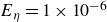 $E_\eta =1\times 10^{-6}$
, circles represent
$E_\eta =1\times 10^{-6}$
, circles represent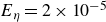 $E_\eta =2\times 10^{-5}$
and triangles represent
$E_\eta =2\times 10^{-5}$
and triangles represent $E_\eta =5\times 10^{-6}$
.
$E_\eta =5\times 10^{-6}$
.

The relation between the resultant local Rayleigh number $ \textit{Ra}_\ell$
and the ratio of frequencies given by
$ \textit{Ra}_\ell$
and the ratio of frequencies given by
 \begin{align} \bigg (\dfrac {\omega _M^2}{\omega _C \omega _\eta }\bigg )_{\!0} \sim \dfrac {V_M^2}{2 \varOmega \eta } \end{align}
is shown in figure 4 for the condition of vanishing slow wave axial kinetic energy for three different values of $E_\eta$
. Each point is obtained by increasing the forcing through
$E_\eta$
. Each point is obtained by increasing the forcing through $ \textit{Ra}_\ell$
and noting the transition from the regime
$ \textit{Ra}_\ell$
and noting the transition from the regime $|\omega _{M}|\gt |\omega _{A}|$
to the regime
$|\omega _{M}|\gt |\omega _{A}|$
to the regime $|\omega _{A}|\gtrsim |\omega _{M}|$
. The resultant forcing needed to suppress the slow MAC waves increases with
$|\omega _{A}|\gtrsim |\omega _{M}|$
. The resultant forcing needed to suppress the slow MAC waves increases with $(\omega _M^2/\omega _C \omega _\eta )_0$
, which is a measure of the square of the peak dimensionless magnetic field in the dynamo (see § 3.4). The linear relation obtained in figure 4 reflects the parity between
$(\omega _M^2/\omega _C \omega _\eta )_0$
, which is a measure of the square of the peak dimensionless magnetic field in the dynamo (see § 3.4). The linear relation obtained in figure 4 reflects the parity between $|\omega _{M}|$
and
$|\omega _{M}|$
and $|\omega _{A}|$
at the state of vanishing slow MAC waves. Since the relative orders of magnitude of the basic frequencies do not depend on the orientation of the gravity, rotation and magnetic field axes, the Cartesian model serves as the basis for the study of the role of equatorially anti-symmetric boundary heat flux in the nonlinear dynamo in § 3, where the state of vanishing slow waves is shown to be a proxy for polarity transitions. We anticipate a self-similar behaviour for the dipole–multipole transition in the dynamo, where both
$|\omega _{A}|$
at the state of vanishing slow MAC waves. Since the relative orders of magnitude of the basic frequencies do not depend on the orientation of the gravity, rotation and magnetic field axes, the Cartesian model serves as the basis for the study of the role of equatorially anti-symmetric boundary heat flux in the nonlinear dynamo in § 3, where the state of vanishing slow waves is shown to be a proxy for polarity transitions. We anticipate a self-similar behaviour for the dipole–multipole transition in the dynamo, where both $ \textit{Ra}_\ell$
and the square of the peak magnetic field are measurable quantities.
$ \textit{Ra}_\ell$
and the square of the peak magnetic field are measurable quantities.
3. Nonlinear dynamo simulations
We consider an electrically conducting fluid confined between two concentric, co-rotating spherical surfaces. The ratio of the inner radius to the outer radius is 0.35. Fluid motion is driven by thermal buoyancy-driven convection. Lengths are scaled by the depth of the spherical shell $L$
and time is scaled by magnetic diffusion time
$L$
and time is scaled by magnetic diffusion time $L^2/\eta$
. The velocity
$L^2/\eta$
. The velocity $\boldsymbol{u}$
and magnetic field
$\boldsymbol{u}$
and magnetic field $\boldsymbol{B}$
are scaled by
$\boldsymbol{B}$
are scaled by $\eta /L$
and
$\eta /L$
and $(2\varOmega \rho \mu \eta )^{1/2}$
, respectively. The temperature is scaled by
$(2\varOmega \rho \mu \eta )^{1/2}$
, respectively. The temperature is scaled by $\beta _s L$
, where
$\beta _s L$
, where $\beta _s$
is the mean equatorial radial temperature gradient within the shell. In the Boussinesq approximation, the non-dimensional magnetohydrodynamic (MHD) equations for velocity, magnetic field and temperature are as follows:
$\beta _s$
is the mean equatorial radial temperature gradient within the shell. In the Boussinesq approximation, the non-dimensional magnetohydrodynamic (MHD) equations for velocity, magnetic field and temperature are as follows:
 \begin{align} E \textit{Pm}^{-1} \Bigl (\frac {\partial {\boldsymbol u}}{\partial t} + (\boldsymbol{\nabla }\times {\boldsymbol u}) \times {\boldsymbol u} \Bigr )+ \hat {\boldsymbol{e}}_z \times {\boldsymbol u} = - \boldsymbol{\nabla }p^\star + \textit{Ra}_V \, \textit{Pm} \textit{Pr}^{-1} \, T \, {\boldsymbol r} \, \nonumber \\ + (\boldsymbol{\nabla }\times {\boldsymbol B}) \times {\boldsymbol B} + E{\nabla} ^2 {\boldsymbol u}, \\[-28pt] \nonumber \end{align}
 \begin{align} \frac {\partial {\boldsymbol B}}{\partial t} = \boldsymbol{\nabla }\times ({\boldsymbol u} \times {\boldsymbol B}) + {\nabla} ^2 {\boldsymbol B}, \\[-28pt] \nonumber \end{align}
 \begin{align} \frac {\partial T}{\partial t} +({\boldsymbol u} \boldsymbol{\cdot }\boldsymbol{\nabla }) T = \textit{Pm} \textit{Pr}^{-1} \, {\nabla} ^2 T, \\[-28pt] \nonumber \end{align}
 \begin{align} \boldsymbol{\nabla }\boldsymbol{\cdot }{\boldsymbol u} = \boldsymbol{\nabla }\boldsymbol{\cdot }{\boldsymbol B} = 0. \\[0pt] \nonumber \end{align}
The modified pressure $p^*$
in (3.1) is given by
$p^*$
in (3.1) is given by $p+ ( 1/{2} )E \, \textit{Pm}^{-1} \, |\boldsymbol{u}|^2$
. The dimensionless parameters in the previous equations are the Ekman number
$p+ ( 1/{2} )E \, \textit{Pm}^{-1} \, |\boldsymbol{u}|^2$
. The dimensionless parameters in the previous equations are the Ekman number $E=\nu /2\varOmega L^2$
, the Prandtl number
$E=\nu /2\varOmega L^2$
, the Prandtl number $ \textit{Pr}=\nu /\kappa$
, the magnetic Prandtl number
$ \textit{Pr}=\nu /\kappa$
, the magnetic Prandtl number $ \textit{Pm}=\nu /\eta$
and the modified vertical Rayleigh number
$ \textit{Pm}=\nu /\eta$
and the modified vertical Rayleigh number $ \textit{Ra}_V=g \alpha \beta _s L^2/2 \varOmega \kappa$
. Here,
$ \textit{Ra}_V=g \alpha \beta _s L^2/2 \varOmega \kappa$
. Here, $g$
is the gravitational acceleration,
$g$
is the gravitational acceleration, $\nu$
is the kinematic viscosity,
$\nu$
is the kinematic viscosity, $\kappa$
is the thermal diffusivity and
$\kappa$
is the thermal diffusivity and $\alpha$
is the coefficient of thermal expansion. The basic state conductive temperature profile is one of basal heating, given by
$\alpha$
is the coefficient of thermal expansion. The basic state conductive temperature profile is one of basal heating, given by $T_0(r) = r_i r_o/r$
, where
$T_0(r) = r_i r_o/r$
, where $r_i$
and
$r_i$
and $r_o$
are the inner and outer radii of the spherical shell. The velocity and magnetic fields satisfy the no-slip and electrically insulating conditions, respectively, at the two boundaries. The inner boundary is isothermal, while a fixed heat flux at the outer boundary is given as the sum of the uniform mean and a lateral variation. The heterogeneity at the outer boundary is measured by the ratio
$r_o$
are the inner and outer radii of the spherical shell. The velocity and magnetic fields satisfy the no-slip and electrically insulating conditions, respectively, at the two boundaries. The inner boundary is isothermal, while a fixed heat flux at the outer boundary is given as the sum of the uniform mean and a lateral variation. The heterogeneity at the outer boundary is measured by the ratio
 \begin{align} q^*=\frac {\text{Maximum heat flux variation}} {\text{Mean heat flux}}. \end{align}
The mean basic state heat flux in the denominator of (3.5) represents the superadiabatic heat flux from the core (e.g. Olson et al. Reference Olson, Deguen, Rudolph and Zhong2015, p. 11). The maximum heat flux variation at the outer boundary represents the magnitude of the peak-to-peak variation at the CMB relative to the mean superadiabatic value. The calculations are performed by a pseudospectral code that uses spherical harmonic expansions in the angular coordinates $(\theta ,\phi )$
and finite differences in radius
$(\theta ,\phi )$
and finite differences in radius $r$
(Willis, Sreenivasan & Gubbins Reference Willis, Sreenivasan and Gubbins2007).
$r$
(Willis, Sreenivasan & Gubbins Reference Willis, Sreenivasan and Gubbins2007).
The parameter space in focus is that of low inertia, wherein the Rossby number based on the characteristic length scale of convection, $Ro_\ell$
(Christensen & Aubert Reference Christensen and Aubert2006), is small. Two Ekman numbers are considered, with the value of
$Ro_\ell$
(Christensen & Aubert Reference Christensen and Aubert2006), is small. Two Ekman numbers are considered, with the value of $ \textit{Pm} = \textit{Pr}$
set to keep
$ \textit{Pm} = \textit{Pr}$
set to keep $Ro_\ell \ll 0.1$
, ensuring that the simulations remain in the low-inertia regime. We explore the effect of inhomogeneous heat flux boundary conditions at the outer boundary on the dipole–multipole transition. To this end, we progressively increase the magnitude of the heat flux heterogeneity at the outer boundary for a given
$Ro_\ell \ll 0.1$
, ensuring that the simulations remain in the low-inertia regime. We explore the effect of inhomogeneous heat flux boundary conditions at the outer boundary on the dipole–multipole transition. To this end, we progressively increase the magnitude of the heat flux heterogeneity at the outer boundary for a given $ \textit{Ra}_V$
. For a given
$ \textit{Ra}_V$
. For a given $q^*$
, the critical vertical Rayleigh number for the onset of non-magnetic convection,
$q^*$
, the critical vertical Rayleigh number for the onset of non-magnetic convection, $ \textit{Ra}_{V,\, c}$
, is obtained for neutral stability of the perturbations subject to a steady mean flow and temperature field produced by the heterogeneity (Sahoo & Sreenivasan Reference Sahoo and Sreenivasan2017). The ratio
$ \textit{Ra}_{V,\, c}$
, is obtained for neutral stability of the perturbations subject to a steady mean flow and temperature field produced by the heterogeneity (Sahoo & Sreenivasan Reference Sahoo and Sreenivasan2017). The ratio $ \textit{Ra}_V/Ra_{V,\, c}$
(table 1) is a measure of the supercriticality of convection.
$ \textit{Ra}_V/Ra_{V,\, c}$
(table 1) is a measure of the supercriticality of convection.
The mean spherical harmonic degrees for convection and energy injection, denoted by $l_{c}$
(Christensen & Aubert Reference Christensen and Aubert2006) and
$l_{c}$
(Christensen & Aubert Reference Christensen and Aubert2006) and $l_{E}$
(Sreenivasan, Sahoo & Dhama Reference Sreenivasan, Sahoo and Dhama2014; Varma & Sreenivasan Reference Varma and Sreenivasan2022; Majumder et al. Reference Majumder, Sreenivasan and Maurya2024), respectively, are given by
$l_{E}$
(Sreenivasan, Sahoo & Dhama Reference Sreenivasan, Sahoo and Dhama2014; Varma & Sreenivasan Reference Varma and Sreenivasan2022; Majumder et al. Reference Majumder, Sreenivasan and Maurya2024), respectively, are given by
 \begin{align} l_{c}= \dfrac {\varSigma \hspace {1pt} l \hspace {1pt} E_{k}(l)} {\varSigma \hspace {1pt} E_{k}(l)}; \quad l_{E}= \dfrac {\varSigma \hspace {1pt} l \hspace {1pt} E_{T}(l)}{\varSigma \hspace {1pt} E_{T}(l)}, \end{align}
where $E_{k}(l)$
is the kinetic energy spectrum, and
$E_{k}(l)$
is the kinetic energy spectrum, and $E_{T}(l)$
is the spectrum obtained from the product of the transform of
$E_{T}(l)$
is the spectrum obtained from the product of the transform of $u_{r}T$
and its conjugate, showing the spectral distribution of scales at which energy is injected by buoyancy. The total kinetic and magnetic energies in the saturated dynamo are given by the volume integrals
$u_{r}T$
and its conjugate, showing the spectral distribution of scales at which energy is injected by buoyancy. The total kinetic and magnetic energies in the saturated dynamo are given by the volume integrals
 \begin{align} E_k= \dfrac {1}{2} \int \boldsymbol{u}^2 \,\mbox{d}V; \quad E_m= \dfrac {\textit{Pm}}{2E} \int \boldsymbol{B}^2\, \mbox{d}V. \end{align}
The relative dipole field strength $f_{\textit{dip}}$
, which is the ratio of the mean dipole field strength to the field strength in harmonic degrees
$f_{\textit{dip}}$
, which is the ratio of the mean dipole field strength to the field strength in harmonic degrees $l =$
1–12 at the outer boundary (Christensen & Aubert Reference Christensen and Aubert2006), takes values
$l =$
1–12 at the outer boundary (Christensen & Aubert Reference Christensen and Aubert2006), takes values ${\gt } 0.35$
in all the dipole-dominated runs (see table 1).
${\gt } 0.35$
in all the dipole-dominated runs (see table 1).
The square of the peak magnetic field, denoted by $B^2_{\textit{peak}}$
(tables 1 and 2), is obtained from the time-averaged value of the magnetic field at the peak-field location in the saturated state of each run.
$B^2_{\textit{peak}}$
(tables 1 and 2), is obtained from the time-averaged value of the magnetic field at the peak-field location in the saturated state of each run.
For caption see next page.

(cntd). Summary of the main input and output parameters of a few dynamo simulations. Here, $ \textit{Ra}_V$
is the modified vertical Rayleigh number,
$ \textit{Ra}_V$
is the modified vertical Rayleigh number, $ \textit{Ra}_{V,\, c}$
is the modified vertical critical Rayleigh number for onset of nonmagnetic convection,
$ \textit{Ra}_{V,\, c}$
is the modified vertical critical Rayleigh number for onset of nonmagnetic convection, $q^*$
is a dimensionless measure of the boundary heterogeneity defined in (3.5),
$q^*$
is a dimensionless measure of the boundary heterogeneity defined in (3.5), $N_r$
is the number of radial grid points,
$N_r$
is the number of radial grid points, $l_{max }$
is the maximum spherical harmonic degree,
$l_{max }$
is the maximum spherical harmonic degree, $Rm$
is the magnetic Reynolds number,
$Rm$
is the magnetic Reynolds number, $Ro_\ell$
is the local Rossby number,
$Ro_\ell$
is the local Rossby number, $l_C$
and
$l_C$
and $l_E$
are the mean spherical harmonic degrees of convection and energy injection respectively,
$l_E$
are the mean spherical harmonic degrees of convection and energy injection respectively, $\overline {m}$
is the mean spherical harmonic order in the range
$\overline {m}$
is the mean spherical harmonic order in the range $l \leqslant l_E$
,
$l \leqslant l_E$
, $\bar {k}_s$
and
$\bar {k}_s$
and $\bar {k}_z$
are the mean
$\bar {k}_z$
are the mean $s$
and
$s$
and $z$
wavenumbers in the range
$z$
wavenumbers in the range $l \leqslant l_E$
,
$l \leqslant l_E$
, $E_k$
and
$E_k$
and $E_m$
are the time-averaged total kinetic and magnetic energies,
$E_m$
are the time-averaged total kinetic and magnetic energies, $f_{\textit{dip}}$
is the relative dipole field strength,
$f_{\textit{dip}}$
is the relative dipole field strength, $ \textit{Ra}_{\ell ,H}/Ra_\ell$
is the ratio of the local horizontal to the resultant Rayleigh numbers (obtained from (3.15) and (3.16)), and
$ \textit{Ra}_{\ell ,H}/Ra_\ell$
is the ratio of the local horizontal to the resultant Rayleigh numbers (obtained from (3.15) and (3.16)), and $B^2_{\textit{rms}}$
is the measured root mean square value of the field in the spherical shell. Types ‘D’, ‘R’ and ‘M’ denote dipolar, reversing and multipolar dynamo states, respectively. The other dynamo parameters are
$B^2_{\textit{rms}}$
is the measured root mean square value of the field in the spherical shell. Types ‘D’, ‘R’ and ‘M’ denote dipolar, reversing and multipolar dynamo states, respectively. The other dynamo parameters are $E = 1.2 \times 10^{-5}$
,
$E = 1.2 \times 10^{-5}$
, $ \textit{Pm} = \textit{Pr} = 1$
.
$ \textit{Pm} = \textit{Pr} = 1$
.
For caption see next page.

(cntd). Summary of the main input and output parameters in the reversing dynamo simulations considered in this study for $Y_2^1$
heat flux condition. These simulations have
$Y_2^1$
heat flux condition. These simulations have $|\omega _{A}/\omega _{M}|\geq 1$
throughout. Here,
$|\omega _{A}/\omega _{M}|\geq 1$
throughout. Here, $ \textit{Ra}_V$
is the modified Rayleigh number,
$ \textit{Ra}_V$
is the modified Rayleigh number, $ \textit{Ra}_{V,\, c}$
is the modified vertical critical Rayleigh number for onset of nonmagnetic convection,
$ \textit{Ra}_{V,\, c}$
is the modified vertical critical Rayleigh number for onset of nonmagnetic convection, $q^*$
is a dimensionless measure of the boundary heterogeneity defined in (3.5),
$q^*$
is a dimensionless measure of the boundary heterogeneity defined in (3.5), $N_r$
is the number of radial grid points,
$N_r$
is the number of radial grid points, $l_{\textit{max}}$
is the maximum spherical harmonic degree,
$l_{\textit{max}}$
is the maximum spherical harmonic degree, $Rm$
is the magnetic Reynolds number,
$Rm$
is the magnetic Reynolds number, $Ro_\ell$
is the local Rossby number,
$Ro_\ell$
is the local Rossby number, $l_C$
and
$l_C$
and $l_E$
are the mean spherical harmonic degrees of convection and energy injection, respectively (defined in (3.6)),
$l_E$
are the mean spherical harmonic degrees of convection and energy injection, respectively (defined in (3.6)), $\overline {m}$
is the mean spherical harmonic order in the range
$\overline {m}$
is the mean spherical harmonic order in the range $l \leqslant l_E$
,
$l \leqslant l_E$
, $\bar {k}_s$
and
$\bar {k}_s$
and $\bar {k}_z$
are the mean
$\bar {k}_z$
are the mean $s$
and
$s$
and $z$
wavenumbers in the range
$z$
wavenumbers in the range $l \leqslant l_E$
,
$l \leqslant l_E$
, $E_k$
and
$E_k$
and $E_m$
are the time-averaged total kinetic and magnetic energies defined in (3.7)
$E_m$
are the time-averaged total kinetic and magnetic energies defined in (3.7) $B^2_{\textit{rms}}$
is the measured mean square value of the field in the spherical shell,
$B^2_{\textit{rms}}$
is the measured mean square value of the field in the spherical shell, $f_{\textit{dip}}$
is the relative dipole field strength,
$f_{\textit{dip}}$
is the relative dipole field strength, $ \textit{Ra}_\ell$
is the local Rayleigh number defined in (3.15), and
$ \textit{Ra}_\ell$
is the local Rayleigh number defined in (3.15), and $B^2_{\textit{peak}}$
is the square of the measured peak field when slow MAC waves cease to exist when
$B^2_{\textit{peak}}$
is the square of the measured peak field when slow MAC waves cease to exist when $|\omega _{A}|\approx |\omega _{M}|$
.
$|\omega _{A}|\approx |\omega _{M}|$
.
3.1. Effect of equatorially symmetric and anti-symmetric heat flux patterns on polarity transitions
We begin our simulations with a strong field dynamo ( $B^2_{\textit{rms}} \gt 1$
) and increase the heterogeneity of the heat flux at the outer boundary in steps while keeping all other parameters fixed. Figure 5(a–d) gives examples of the equatorially anti-symmetric, symmetric and composite boundary conditions whose effects on polarity transitions are analysed in this study. The simulations are performed for at least one magnetic diffusion time in the saturated state.
$B^2_{\textit{rms}} \gt 1$
) and increase the heterogeneity of the heat flux at the outer boundary in steps while keeping all other parameters fixed. Figure 5(a–d) gives examples of the equatorially anti-symmetric, symmetric and composite boundary conditions whose effects on polarity transitions are analysed in this study. The simulations are performed for at least one magnetic diffusion time in the saturated state.
In figure 6, the colatitude of the axial dipole field, $\theta$
, at the outer boundary is obtained from the Gauss coefficients of the spherical harmonics, as follows:
$\theta$
, at the outer boundary is obtained from the Gauss coefficients of the spherical harmonics, as follows:
 \begin{align} \cos \theta = g_1^0/|\boldsymbol{m}|, \quad \boldsymbol{m} = \big(g_1^0, g_1^1, h_1^1 \big), \end{align}
where $g_1^0$
,
$g_1^0$
, $g_1^1$
and
$g_1^1$
and $h_1^1$
are derived from the Schmidt-normalised expansion for the scalar potential of the field (Glatzmaier Reference Glatzmaier2013, pp. 142–143).
$h_1^1$
are derived from the Schmidt-normalised expansion for the scalar potential of the field (Glatzmaier Reference Glatzmaier2013, pp. 142–143).
Distribution of heterogeneous radial temperature gradient $\partial T/\partial r$
at the outer boundary for different conditions: (a)
$\partial T/\partial r$
at the outer boundary for different conditions: (a) $Y_2^1$
; (b)
$Y_2^1$
; (b) $Y^2_2$
; (c)
$Y^2_2$
; (c) $Y_2^2:Y_2^1=2:1$
; and (d) tomographic condition derived from the seismic shear wave velocity variation in the Earth’s lower mantle (Masters et al. Reference Masters, Johnson, Laske and Bolton1996).
$Y_2^2:Y_2^1=2:1$
; and (d) tomographic condition derived from the seismic shear wave velocity variation in the Earth’s lower mantle (Masters et al. Reference Masters, Johnson, Laske and Bolton1996).

For $E = 1.2 \times 10^{-5}$
,
$E = 1.2 \times 10^{-5}$
, $ \textit{Pm} = \textit{Pr} = 1$
and
$ \textit{Pm} = \textit{Pr} = 1$
and $ \textit{Ra}_V = 2500$
, a strong dipole-dominated dynamo undergoes well-defined polarity reversals, as shown in figure 6(b), by progressively increasing
$ \textit{Ra}_V = 2500$
, a strong dipole-dominated dynamo undergoes well-defined polarity reversals, as shown in figure 6(b), by progressively increasing $q^*$
for the equatorially anti-symmetric
$q^*$
for the equatorially anti-symmetric $Y_2^1$
heat flux pattern. With a further increase in
$Y_2^1$
heat flux pattern. With a further increase in $q^*$
, the dynamo exhibits a multipolar solution (figure 6
c). However, the equatorially symmetric
$q^*$
, the dynamo exhibits a multipolar solution (figure 6
c). However, the equatorially symmetric $Y_2^2$
heat flux pattern does not produce polarity transitions even with a strong heterogeneity (see figure 6
d). For the same parameters, the Earth-like composite heat flux pattern in figure 5(d), which consists of both symmetric and anti-symmetric parts, produces polarity transitions. From the evolution of the dipole axis tilt (figure 17, Appendix A), well-defined polarity reversals are noted for
$Y_2^2$
heat flux pattern does not produce polarity transitions even with a strong heterogeneity (see figure 6
d). For the same parameters, the Earth-like composite heat flux pattern in figure 5(d), which consists of both symmetric and anti-symmetric parts, produces polarity transitions. From the evolution of the dipole axis tilt (figure 17, Appendix A), well-defined polarity reversals are noted for $q^*=13$
. For the anti-symmetric
$q^*=13$
. For the anti-symmetric $Y_2^1$
boundary heat flux variation, the radial magnetic fields in the dipolar, reversing and multipolar states are shown in figure 7 for two series with different vertical thermal forcing. In table 1, the runs for two values of
$Y_2^1$
boundary heat flux variation, the radial magnetic fields in the dipolar, reversing and multipolar states are shown in figure 7 for two series with different vertical thermal forcing. In table 1, the runs for two values of $ \textit{Ra}_V$
,
$ \textit{Ra}_V$
, $2500$
and
$2500$
and $20000$
, are presented with different heat flux patterns. In the reversing runs, the ratio of magnetic to kinetic energy
$20000$
, are presented with different heat flux patterns. In the reversing runs, the ratio of magnetic to kinetic energy $E_m/E_k$
falls below unity, as noted in earlier studies (Kutzner & Christensen Reference Kutzner and Christensen2002; Tassin, Gastine & Fournier Reference Tassin, Gastine and Fournier2021) although a recent study (Frasson et al. Reference Frasson, Schaeffer, Nataf and Labrosse2025) suggests that multipolar solutions can exist for
$E_m/E_k$
falls below unity, as noted in earlier studies (Kutzner & Christensen Reference Kutzner and Christensen2002; Tassin, Gastine & Fournier Reference Tassin, Gastine and Fournier2021) although a recent study (Frasson et al. Reference Frasson, Schaeffer, Nataf and Labrosse2025) suggests that multipolar solutions can exist for $E_m/E_k\gt 1$
. Reversing dynamo models in general have not realised
$E_m/E_k\gt 1$
. Reversing dynamo models in general have not realised $E_m/E_k \gt 1$
probably because their magnetic Ekman number
$E_m/E_k \gt 1$
probably because their magnetic Ekman number $E_\eta$
is much higher than that in the Earth’s core in the relatively small length scales. In contrast, the criterion of vanishing slow MAC wave helicity considered in this study applies to the energy-containing scales where density perturbations are continually produced and is independent of the choice of
$E_\eta$
is much higher than that in the Earth’s core in the relatively small length scales. In contrast, the criterion of vanishing slow MAC wave helicity considered in this study applies to the energy-containing scales where density perturbations are continually produced and is independent of the choice of $E_\eta$
in the low-inertia limit that rapidly rotating planets operate in.
$E_\eta$
in the low-inertia limit that rapidly rotating planets operate in.
Evolution of dipole colatitude with magnetic diffusion time for (a) $q^*=17$
,
$q^*=17$
, $Y_2^1$
(stable dipolar), (b)
$Y_2^1$
(stable dipolar), (b) $q^*=18$
,
$q^*=18$
, $Y_2^1$
(reversing), (c)
$Y_2^1$
(reversing), (c) $q^*=20$
,
$q^*=20$
, $Y_2^1$
(multipolar), and (d)
$Y_2^1$
(multipolar), and (d) $q^*=18$
and
$q^*=18$
and $30$
,
$30$
, $Y_2^2$
(stable dipolar). The other dynamo parameters are
$Y_2^2$
(stable dipolar). The other dynamo parameters are $ \textit{Ra}_V = 2500$
,
$ \textit{Ra}_V = 2500$
, $E = 1.2 \times 10^{-5}$
,
$E = 1.2 \times 10^{-5}$
, $ \textit{Pm} = \textit{Pr} = 1$
.
$ \textit{Pm} = \textit{Pr} = 1$
.

Contours of the radial magnetic field at the outer boundary for $ \textit{Ra}_V = 2500$
at
$ \textit{Ra}_V = 2500$
at $q^* =\,(a)\, 17$
, (b) 18, (c) 20; and for
$q^* =\,(a)\, 17$
, (b) 18, (c) 20; and for $ \textit{Ra}_V =25\,000$
at
$ \textit{Ra}_V =25\,000$
at $q^* =\,(d)\, 5$
, (e) 6, (f) 7. The other dynamo parameters are
$q^* =\,(d)\, 5$
, (e) 6, (f) 7. The other dynamo parameters are $E = 1.2 \times 10^{-5}$
,
$E = 1.2 \times 10^{-5}$
, $ \textit{Pm} = \textit{Pr} = 1$
. A
$ \textit{Pm} = \textit{Pr} = 1$
. A $Y_2^1$
heat flux heterogeneity is applied at the outer boundary.
$Y_2^1$
heat flux heterogeneity is applied at the outer boundary.

The main output parameters of the polarity-reversing dynamo runs with the anti-symmetric $Y_2^1$
heat flux boundary condition are reported in table 2. The ratio of anti-symmetric to total kinetic energy remains nearly constant even at high
$Y_2^1$
heat flux boundary condition are reported in table 2. The ratio of anti-symmetric to total kinetic energy remains nearly constant even at high $q^*$
(figure 8), so equatorially anti-symmetric boundary conditions do not induce polarity transitions by breaking the equatorial symmetry of the convection columns. Before analysing the role of wave motions in polarity transitions, we examine the mean temperature and velocity fields produced by the heterogeneous boundary heat flux, which give useful comparisons with the linear convection model.
$q^*$
(figure 8), so equatorially anti-symmetric boundary conditions do not induce polarity transitions by breaking the equatorial symmetry of the convection columns. Before analysing the role of wave motions in polarity transitions, we examine the mean temperature and velocity fields produced by the heterogeneous boundary heat flux, which give useful comparisons with the linear convection model.
Ratio of anti-symmetric to total kinetic energy for $q^*=0$
(black),
$q^*=0$
(black), $q^*=15$
(red),
$q^*=15$
(red), $q^*=18$
(blue) and
$q^*=18$
(blue) and $q^*=20$
(green) with the
$q^*=20$
(green) with the $Y_2^1$
heat flux heterogeneity at the outer boundary. The other dynamo parameters are
$Y_2^1$
heat flux heterogeneity at the outer boundary. The other dynamo parameters are $ \textit{Ra}=2500,\ E = 1.2 \times 10^{-5},\ \textit{Pm}=Pr=1$
.
$ \textit{Ra}=2500,\ E = 1.2 \times 10^{-5},\ \textit{Pm}=Pr=1$
.

3.2. Mean resultant temperature gradient and velocity field
In line with that obtained in (2.35) in the Cartesian model, the mean (superadiabatic) resultant temperature gradient is given by
 \begin{align} \beta = \beta _s - 2 \beta _z k_s/k_z, \end{align}
where $\beta _s = \partial T_0/\partial s \lt 0$
in an unstably stratified layer with homogeneous boundary heat flux (see figure 9
a). In figure 9(b),
$\beta _s = \partial T_0/\partial s \lt 0$
in an unstably stratified layer with homogeneous boundary heat flux (see figure 9
a). In figure 9(b), $\beta _z = \partial T_0/\partial z$
is plotted for an equatorially antisymmetric
$\beta _z = \partial T_0/\partial z$
is plotted for an equatorially antisymmetric $Y_2^1$
heat-flux heterogeneity at the outer boundary. The temperature gradients are calculated from a steady state just below non-magnetic convective onset (
$Y_2^1$
heat-flux heterogeneity at the outer boundary. The temperature gradients are calculated from a steady state just below non-magnetic convective onset ( $ \textit{Ra}_V = 30$
, whereas onset occurs at
$ \textit{Ra}_V = 30$
, whereas onset occurs at $ \textit{Ra}_V = 31$
for
$ \textit{Ra}_V = 31$
for $q^* = 18$
) so that the perturbations do not affect the calculation of the mean gradients. An averaged
$q^* = 18$
) so that the perturbations do not affect the calculation of the mean gradients. An averaged $\beta _z$
, obtained by taking the average of the positively signed
$\beta _z$
, obtained by taking the average of the positively signed $\partial T_0/\partial z$
within the spherical shell, is proportional to the intensity of the anti-symmetric heterogeneity. Likewise, the averaged
$\partial T_0/\partial z$
within the spherical shell, is proportional to the intensity of the anti-symmetric heterogeneity. Likewise, the averaged $\beta _s$
is obtained by taking the average of
$\beta _s$
is obtained by taking the average of $\partial T_0/\partial s$
within the shell. The averaged resultant gradient
$\partial T_0/\partial s$
within the shell. The averaged resultant gradient $\beta$
is then evaluated from (3.9) using the average
$\beta$
is then evaluated from (3.9) using the average $s$
and
$s$
and $z$
wavenumbers defined in (3.13) (see figure 9
d). The resultant
$z$
wavenumbers defined in (3.13) (see figure 9
d). The resultant $\beta$
calculated at
$\beta$
calculated at $ \textit{Ra}_V = 30$
and the resultant
$ \textit{Ra}_V = 30$
and the resultant $\beta$
averaged over
$\beta$
averaged over ${\sim}0.5$
diffusion time from the strongly supercritical state at
${\sim}0.5$
diffusion time from the strongly supercritical state at $ \textit{Ra}_V=310$
exhibit similar structures as well as nearly equal maximum and minimum values (see supplementary figure S4). Convection is suppressed in stably stratified regions where
$ \textit{Ra}_V=310$
exhibit similar structures as well as nearly equal maximum and minimum values (see supplementary figure S4). Convection is suppressed in stably stratified regions where $\partial T/\partial r \gt 0$
, whereas regions with
$\partial T/\partial r \gt 0$
, whereas regions with $\partial T/\partial r \lt 0$
support convection (see figure 9
f). Within the convective region,
$\partial T/\partial r \lt 0$
support convection (see figure 9
f). Within the convective region, $\beta _z \gt 0$
below the equatorial plane, while
$\beta _z \gt 0$
below the equatorial plane, while $\beta _z \lt 0$
above the equator. Consistent with the Cartesian model in § 2, where the positively signed
$\beta _z \lt 0$
above the equator. Consistent with the Cartesian model in § 2, where the positively signed $\beta _z$
is symmetric about the mid-plane
$\beta _z$
is symmetric about the mid-plane $z = 0$
, the equatorially anti-symmetric boundary condition yields a
$z = 0$
, the equatorially anti-symmetric boundary condition yields a $\beta _z$
that is symmetric about the equator, which is then used to compute the resultant
$\beta _z$
that is symmetric about the equator, which is then used to compute the resultant $\beta$
. The unstably stratified region is in focus in the analysis in § 3.3 – at moderately positive values of
$\beta$
. The unstably stratified region is in focus in the analysis in § 3.3 – at moderately positive values of $\beta _z$
, both fast and slow MAC waves are present, giving the dipolar dynamo regime; at large positive values of
$\beta _z$
, both fast and slow MAC waves are present, giving the dipolar dynamo regime; at large positive values of $\beta _z$
, the slow MAC waves are selectively suppressed whereas the fast MAC waves persist, giving the reversing and multipolar dynamo regimes.
$\beta _z$
, the slow MAC waves are selectively suppressed whereas the fast MAC waves persist, giving the reversing and multipolar dynamo regimes.
Horizontal section plots at $z = 0.4$
below the equator showing (a)
$z = 0.4$
below the equator showing (a) $\beta _s$
for homogeneous boundary heating, (b)
$\beta _s$
for homogeneous boundary heating, (b) $\beta _z$
for
$\beta _z$
for $q^* = 18$
, (c)
$q^* = 18$
, (c) $\beta _\phi$
for
$\beta _\phi$
for $q^* = 18$
and (d) resultant gradient
$q^* = 18$
and (d) resultant gradient $\beta$
for
$\beta$
for $q^* = 18$
. The temperature gradients are calculated at vertical Rayleigh number
$q^* = 18$
. The temperature gradients are calculated at vertical Rayleigh number $ \textit{Ra}_V = 30$
, which is a state near the onset of non-magnetic convection. A
$ \textit{Ra}_V = 30$
, which is a state near the onset of non-magnetic convection. A $Y_2^1$
heterogeneity in outer boundary heat flux is applied. The orange-green coloured strip at the periphery of panel(b) represents
$Y_2^1$
heterogeneity in outer boundary heat flux is applied. The orange-green coloured strip at the periphery of panel(b) represents $\partial T_0 / \partial r$
at the outer boundary. Panels (e) and (f) show snapshots of the axial velocity
$\partial T_0 / \partial r$
at the outer boundary. Panels (e) and (f) show snapshots of the axial velocity $u_z$
at
$u_z$
at $q^* = 0$
and
$q^* = 0$
and $q^* = 18$
, respectively, for dynamo simulations at
$q^* = 18$
, respectively, for dynamo simulations at $ \textit{Ra}_V = 2500$
. The other parameters are
$ \textit{Ra}_V = 2500$
. The other parameters are $ E = 1.2 \times 10^{-5}$
and
$ E = 1.2 \times 10^{-5}$
and $ \textit{Pm} = \textit{Pr} = 1$
.
$ \textit{Pm} = \textit{Pr} = 1$
.

(a) Values of $\beta _s$
(blue),
$\beta _s$
(blue), $\beta _z$
(red) and the resultant
$\beta _z$
(red) and the resultant $\beta$
(black) at cylindrical radius
$\beta$
(black) at cylindrical radius $s = 1$
at the section
$s = 1$
at the section $z = 0.4$
below the equator for
$z = 0.4$
below the equator for $q^* = 18$
. (b) Meridional sections plot of the
$q^* = 18$
. (b) Meridional sections plot of the $\phi$
-component of the velocity,
$\phi$
-component of the velocity, $u_0$
for
$u_0$
for $q^* = 18$
. The plot shows
$q^* = 18$
. The plot shows $\phi$
-averaged values of
$\phi$
-averaged values of $u_0$
in the unstably stratified region where
$u_0$
in the unstably stratified region where $\beta \lt 0$
(
$\beta \lt 0$
( $\phi = 1.31 \, \pi$
to
$\phi = 1.31 \, \pi$
to $0.31 \, \pi$
through
$0.31 \, \pi$
through $\phi =0$
) in the grey-shaded region of panel (a). (c) Values of
$\phi =0$
) in the grey-shaded region of panel (a). (c) Values of $u_0$
along a vertical line passing through cylindrical radius
$u_0$
along a vertical line passing through cylindrical radius $s = 1$
(circles) are compared with the theoretical dimensionless thermal wind in (3.10). The parameters are
$s = 1$
(circles) are compared with the theoretical dimensionless thermal wind in (3.10). The parameters are $ \textit{Ra}_V = 30$
(below onset),
$ \textit{Ra}_V = 30$
(below onset), $E = 1.2 \times 10^{-5}$
, and
$E = 1.2 \times 10^{-5}$
, and $ \textit{Pm} = \textit{Pr} = 1$
. A
$ \textit{Pm} = \textit{Pr} = 1$
. A $Y_2^1$
heat flux heterogeneity is applied at the outer boundary.
$Y_2^1$
heat flux heterogeneity is applied at the outer boundary.

Equation (3.9) is derived from the theoretical model described in § 2, which predicts the presence or absence of slow MAC waves subject to the frequency inequality $|\omega _{C}| \gt |\omega _{M}|,|\omega _{A}| \gt |\omega _{\eta }|$
, with slow MAC waves present when
$|\omega _{C}| \gt |\omega _{M}|,|\omega _{A}| \gt |\omega _{\eta }|$
, with slow MAC waves present when $|\omega _{M}| \gt |\omega _{A}|$
and absent when
$|\omega _{M}| \gt |\omega _{A}|$
and absent when $|\omega _{M}| \leqslant |\omega _{A}|$
. The previous frequency inequality does not predict the localised suppression of convection observed in figure 9(f) and can only be applied to regions where convection is present.
$|\omega _{M}| \leqslant |\omega _{A}|$
. The previous frequency inequality does not predict the localised suppression of convection observed in figure 9(f) and can only be applied to regions where convection is present.
Interestingly, $\beta _\phi = \partial T_0/\partial \phi$
(figure 9
c) has practically no influence on
$\beta _\phi = \partial T_0/\partial \phi$
(figure 9
c) has practically no influence on $\beta$
, which justifies our original assumption of ignoring variations with respect to the non-preferred horizontal direction (see (2.14), § 2.2). The convective region produced by
$\beta$
, which justifies our original assumption of ignoring variations with respect to the non-preferred horizontal direction (see (2.14), § 2.2). The convective region produced by $\beta _s \lt 0$
and
$\beta _s \lt 0$
and $\beta _z\gt 0$
with the equatorially anti-symmetric heat flux at the boundary corresponds to the unstably stratified system modelled by the equatorial radial configuration of the Cartesian linear model in § 2.1.
$\beta _z\gt 0$
with the equatorially anti-symmetric heat flux at the boundary corresponds to the unstably stratified system modelled by the equatorial radial configuration of the Cartesian linear model in § 2.1.
Figure 10(a) shows the azimuthal variation of the mean temperature gradients at cylindrical radius $s = 1$
and at the section
$s = 1$
and at the section $z = 0.4$
below the equator for the
$z = 0.4$
below the equator for the $Y_2^1$
heterogeneity with
$Y_2^1$
heterogeneity with $q^* = 18$
. The grey-shaded region indicates
$q^* = 18$
. The grey-shaded region indicates $\beta _z \gt 0$
, where the resultant
$\beta _z \gt 0$
, where the resultant $\beta$
is calculated from (3.9). Figure 10(b) gives the meridional plot of the steady mean flow
$\beta$
is calculated from (3.9). Figure 10(b) gives the meridional plot of the steady mean flow $u_0$
(
$u_0$
( $\phi$
-component of the velocity) averaged over the unstably stratified longitudes in figure 10(a) (
$\phi$
-component of the velocity) averaged over the unstably stratified longitudes in figure 10(a) ( $ \phi = 1.31 \, \pi$
to
$ \phi = 1.31 \, \pi$
to $0.31 \, \pi$
through
$0.31 \, \pi$
through $\phi =0$
). In figure 10(c), the magnitude of this equatorially anti-symmetric flow measured at
$\phi =0$
). In figure 10(c), the magnitude of this equatorially anti-symmetric flow measured at $s=1$
shows a fair agreement with the theoretical value of the thermal wind calculated from (2.3) in dimensionless units,
$s=1$
shows a fair agreement with the theoretical value of the thermal wind calculated from (2.3) in dimensionless units,
 \begin{align} u_0 = -\frac {g \alpha \beta _z L}{2\varOmega \eta } \,z =-Ra_V \, \beta ^* z, \end{align}
where $\beta ^* =\beta _z/\beta _s$
is obtained from the respective averaged temperature gradients.
$\beta ^* =\beta _z/\beta _s$
is obtained from the respective averaged temperature gradients.
3.3. Role of slow MAC waves in the dipole–multipole transition
In § 2, we examined the evolution of an isolated density perturbation in an unstably stratified fluid subject to background rotation, a uniform magnetic field and a horizontal temperature gradient. Perturbations of this kind excite MAC waves in the dynamo, the frequencies of which depend on the fundamental frequencies given as follows:
 \begin{align} \omega _{C}^2 = \frac {4(\boldsymbol{\varOmega } \boldsymbol{\cdot }\boldsymbol{k})^2}{ k^2},\quad \omega _{M}^2 =\frac {(\boldsymbol{B} \boldsymbol{\cdot }\boldsymbol{k})^2}{\mu \rho }, \quad -\omega _{A,V}^2= g\alpha \beta _s \, \frac { k_{h}^2}{k^2}, \quad \omega _{A,H}^2= g\alpha \beta _z \frac { k_{h}^2}{k^2}\frac {k_s}{k_z} \end{align}
and scaling the frequencies by $\eta /L^2$
, we obtain in dimensionless units,
$\eta /L^2$
, we obtain in dimensionless units,
 \begin{align} \omega _C^2 = \frac {\textit{Pm}^2}{E^2} \frac {k_z^2}{k^2}, \!\!\quad \omega _M^2 = \frac {\textit{Pm}}{E} (\boldsymbol{B} \boldsymbol{\cdot }{\boldsymbol k})^2, \!\!\quad -\omega _{A,V}^2 = \frac {\textit{Pm} \textit{Ra}_V}{E} \,\frac {{k_h}^2}{k^2}, \!\!\quad \omega _{A,H}^2 = \frac {\textit{Pm} \textit{Ra}_H}{2 \,E} \,\frac {{k_h}^2}{k^2}, \!\!\quad \end{align}
where $k_s$
,
$k_s$
, $k_{\phi }$
and
$k_{\phi }$
and $k_z$
are the radial, azimuthal and axial wavenumbers in cylindrical coordinates
$k_z$
are the radial, azimuthal and axial wavenumbers in cylindrical coordinates $(s,\phi ,z)$
,
$(s,\phi ,z)$
, $k_\phi =m/s$
, where
$k_\phi =m/s$
, where $m$
is the spherical harmonic order,
$m$
is the spherical harmonic order, $k^2=k_s^2+k_\phi ^2+k_z^2$
and
$k^2=k_s^2+k_\phi ^2+k_z^2$
and $k_h$
is the horizontal wavenumber in the equatorial region defined by
$k_h$
is the horizontal wavenumber in the equatorial region defined by $k_h^2=k_\phi ^2+k_z^2$
. The
$k_h^2=k_\phi ^2+k_z^2$
. The $s$
,
$s$
, $\phi$
and
$\phi$
and $z$
wavenumbers are calculated in the saturated state of the dynamo runs in the energy-containing scales (
$z$
wavenumbers are calculated in the saturated state of the dynamo runs in the energy-containing scales ( $l\leqslant l_E$
). For example, real space integration over
$l\leqslant l_E$
). For example, real space integration over $(s,\phi )$
gives the kinetic energy as a function of
$(s,\phi )$
gives the kinetic energy as a function of $z$
, the Fourier transform of which gives the one-dimensional spectrum
$z$
, the Fourier transform of which gives the one-dimensional spectrum $\hat {u}^2 (k_z)$
. Subsequently, we obtain
$\hat {u}^2 (k_z)$
. Subsequently, we obtain
 \begin{align} \bar {k}_z = \frac {\varSigma k_z \, \hat {u}^2 (k_z)} {\varSigma \hat {u}^2 (k_z)}. \end{align}
A similar approach yields $\bar {k}_s$
and
$\bar {k}_s$
and $\overline {m}$
. The magnetic (Alfvén) wave frequency
$\overline {m}$
. The magnetic (Alfvén) wave frequency $\omega _M$
is based on the three components of the measured magnetic field at the peak-field location. The wavenumber
$\omega _M$
is based on the three components of the measured magnetic field at the peak-field location. The wavenumber $k_\phi$
is evaluated at
$k_\phi$
is evaluated at $s=1$
, approximately mid-radius of the spherical shell. The horizontal Rayleigh number is given by
$s=1$
, approximately mid-radius of the spherical shell. The horizontal Rayleigh number is given by
 \begin{align} \textit{Ra}_H=2 \, \frac {g \alpha \beta _z L^2}{2 \varOmega \eta }\frac {k_s}{k_z}. \end{align}
The local vertical and horizontal Rayleigh numbers in the dynamo based on the flow length scale are given by
 \begin{align} \textit{Ra}_{\ell ,V}=\frac {g \alpha |\beta _s|}{2 \varOmega \eta } \left (\frac {\pi }{k_s}\right )^2,\quad \textit{Ra}_{\ell ,H}=2 \, \frac {g \alpha |\beta _z|}{2 \varOmega \eta } \frac {k_s}{k_z} \left (\frac {\pi }{k_s}\right )^2, \end{align}
and the resultant local Rayleigh number is then
 \begin{align} \textit{Ra}_{\ell }=\textit{Ra}_{\ell ,V} +\textit{Ra}_{\ell ,H}. \end{align}
Variation of the squares of the fundamental frequencies with $q^*$
and
$q^*$
and $ \textit{Ra}_{\ell ,H}/Ra_\ell$
(within brackets) for (a)
$ \textit{Ra}_{\ell ,H}/Ra_\ell$
(within brackets) for (a) $ \textit{Ra}_V=2500$
,
$ \textit{Ra}_V=2500$
, $Y_2^1$
heat flux heterogeneity, and (b)
$Y_2^1$
heat flux heterogeneity, and (b) $ \textit{Ra}_V=2500$
,
$ \textit{Ra}_V=2500$
, $Y_2^2$
heat flux heterogeneity. The dotted vertical line marks the polarity-reversing state that lies between the dipolar and multipolar regimes. The other dynamo parameters are
$Y_2^2$
heat flux heterogeneity. The dotted vertical line marks the polarity-reversing state that lies between the dipolar and multipolar regimes. The other dynamo parameters are $E = 1.2 \times 10^{-5}$
,
$E = 1.2 \times 10^{-5}$
, $ \textit{Pm}=Pr=1$
.
$ \textit{Pm}=Pr=1$
.

In figure 11, the magnitudes of fundamental frequencies are shown as a function of $q^*$
and
$q^*$
and $ \textit{Ra}_{\ell , H}/Ra_\ell$
for heterogeneous heat flux boundary conditions. The frequencies and local Rayleigh numbers are computed from (3.12), (3.15) and (3.16) using the mean values of the wavenumbers as shown in (3.13). In figure 11(a), we begin with a strong field dynamo and increase the
$ \textit{Ra}_{\ell , H}/Ra_\ell$
for heterogeneous heat flux boundary conditions. The frequencies and local Rayleigh numbers are computed from (3.12), (3.15) and (3.16) using the mean values of the wavenumbers as shown in (3.13). In figure 11(a), we begin with a strong field dynamo and increase the $Y_2^1$
heat flux heterogeneity, which is reflected in the horizontal buoyancy frequency
$Y_2^1$
heat flux heterogeneity, which is reflected in the horizontal buoyancy frequency $\omega _{A,H}$
, while keeping the vertical buoyancy constant at
$\omega _{A,H}$
, while keeping the vertical buoyancy constant at $ \textit{Ra}_V=2500$
. The slow MAC waves are present at relatively low
$ \textit{Ra}_V=2500$
. The slow MAC waves are present at relatively low $q^*$
when
$q^*$
when $|\omega _{M}| \gt |\omega _A|$
. In the polarity-reversing state at
$|\omega _{M}| \gt |\omega _A|$
. In the polarity-reversing state at $q^* = 18$
(
$q^* = 18$
( $ \textit{Ra}_{\ell , {H}}/Ra_\ell \approx 0.62$
), the magnitude of the resultant buoyancy frequency
$ \textit{Ra}_{\ell , {H}}/Ra_\ell \approx 0.62$
), the magnitude of the resultant buoyancy frequency $|\omega _A|$
approximately matches that of the Alfvén frequency
$|\omega _A|$
approximately matches that of the Alfvén frequency $|\omega _{M}|$
, causing the slow wave frequency
$|\omega _{M}|$
, causing the slow wave frequency $\omega _{s}$
to go to zero. While the generation of slow MAC waves ceases, the existing slow MAC waves are damped on the time scale
$\omega _{s}$
to go to zero. While the generation of slow MAC waves ceases, the existing slow MAC waves are damped on the time scale $\delta ^2 / \eta$
(see § 2.4), which is much shorter than the magnetic diffusion time
$\delta ^2 / \eta$
(see § 2.4), which is much shorter than the magnetic diffusion time $L^2 / \eta$
because the ratio of the core depth to the length scale of buoyancy disturbances would be
$L^2 / \eta$
because the ratio of the core depth to the length scale of buoyancy disturbances would be $L / \delta \sim 10^2$
(Sreenivasan & Maurya Reference Sreenivasan and Maurya2021). Whether the rapid damping of the slow MAC waves causes the rapid decay of the axial dipole field during a polarity reversal (see figure 6
b) is at present an open question that requires further investigation. The equatorially symmetric
$L / \delta \sim 10^2$
(Sreenivasan & Maurya Reference Sreenivasan and Maurya2021). Whether the rapid damping of the slow MAC waves causes the rapid decay of the axial dipole field during a polarity reversal (see figure 6
b) is at present an open question that requires further investigation. The equatorially symmetric $Y_2^2$
heat flux boundary condition has zero horizontal buoyancy at the equator, and even at large
$Y_2^2$
heat flux boundary condition has zero horizontal buoyancy at the equator, and even at large $q^*$
, the condition
$q^*$
, the condition $|\omega _A| \gt |\omega _{M}|$
is never met (figure 11
b).
$|\omega _A| \gt |\omega _{M}|$
is never met (figure 11
b).
The variation of the parameter $f_{\textit{dip}}$
against
$f_{\textit{dip}}$
against $|\omega _A/\omega _M|$
in figure 12 shows that reversing (R) and multipolar (M) states exist at values of
$|\omega _A/\omega _M|$
in figure 12 shows that reversing (R) and multipolar (M) states exist at values of $f_{\textit{dip}} \leqslant 0.35$
, the proposed lower bound for the existence of dipole-dominated numerical dynamos in the literature.
$f_{\textit{dip}} \leqslant 0.35$
, the proposed lower bound for the existence of dipole-dominated numerical dynamos in the literature.
Variation of $f_{\textit{dip}}$
with
$f_{\textit{dip}}$
with $|\omega _{A}/\omega _{M}|$
for different heat flux boundary conditions at two values of
$|\omega _{A}/\omega _{M}|$
for different heat flux boundary conditions at two values of $ \textit{Ra}_V$
. The vertical dotted line indicates
$ \textit{Ra}_V$
. The vertical dotted line indicates $|\omega _{A}/\omega _{M}| = 1$
, while the horizontal dotted line marks
$|\omega _{A}/\omega _{M}| = 1$
, while the horizontal dotted line marks $f_{\textit{dip}} = 0.35$
, which has been proposed as the lower bound for the existence of dipole-dominated numerical dynamos (Christensen & Aubert Reference Christensen and Aubert2006). Types ‘D’, ‘R’ and ‘M’ denote dipolar, reversing and multipolar dynamo states, respectively. The other dynamo parameters are
$f_{\textit{dip}} = 0.35$
, which has been proposed as the lower bound for the existence of dipole-dominated numerical dynamos (Christensen & Aubert Reference Christensen and Aubert2006). Types ‘D’, ‘R’ and ‘M’ denote dipolar, reversing and multipolar dynamo states, respectively. The other dynamo parameters are $E = 1.2 \times 10^{-5}$
and
$E = 1.2 \times 10^{-5}$
and $ \textit{Pm} = \textit{Pr} = 1$
.
$ \textit{Pm} = \textit{Pr} = 1$
.

Panels (a–c) (i) show the absolute values of wave frequencies plotted for the saturated state of the dynamo run: (a) $q^*= 0$
, (b)
$q^*= 0$
, (b) $q^*= 10$
and (c)
$q^*= 10$
and (c) $q^*= 18$
for the
$q^*= 18$
for the $Y_2^1$
heat flux heterogeneity at the outer boundary. The shaded grey area shows the range of scales where the helicity of the dynamo run is greater than that of the equivalent non-magnetic run. Panels (a–c) (ii) show the spectral distribution of the power supplied to the axial dipole, defined in (3.17). The other dynamo parameters are
$Y_2^1$
heat flux heterogeneity at the outer boundary. The shaded grey area shows the range of scales where the helicity of the dynamo run is greater than that of the equivalent non-magnetic run. Panels (a–c) (ii) show the spectral distribution of the power supplied to the axial dipole, defined in (3.17). The other dynamo parameters are $ \textit{Ra}_V=2500$
,
$ \textit{Ra}_V=2500$
, $E = 1.2 \times 10^{-5}$
,
$E = 1.2 \times 10^{-5}$
, $ \textit{Pm}=Pr=1$
.
$ \textit{Pm}=Pr=1$
.

The top row of figure 13 displays the square of the fundamental frequencies for a range of spherical harmonic order $m$
for (a)
$m$
for (a) $q^*=0$
, (b)
$q^*=0$
, (b) $q^*=10$
, and (c)
$q^*=10$
, and (c) $q^*=18$
in the saturated state for the equatorially anti-symmetric
$q^*=18$
in the saturated state for the equatorially anti-symmetric $Y_2^1$
heat flux pattern. Dynamo simulations with
$Y_2^1$
heat flux pattern. Dynamo simulations with $q^* = 0$
and
$q^* = 0$
and $q^* = 10$
exhibit stable axial dipoles while the simulation with
$q^* = 10$
exhibit stable axial dipoles while the simulation with $q^* = 18$
gives a reversing dynamo. The shaded area indicates the range of
$q^* = 18$
gives a reversing dynamo. The shaded area indicates the range of $m$
where the kinetic helicity in the dynamo exceeds that of the equivalent non-magnetic run. (For the governing equations of equivalent non-magnetic run, see Majumder et al. Reference Majumder, Sreenivasan and Maurya2024). The black line represents the square of the slow MAC wave frequency under the condition
$m$
where the kinetic helicity in the dynamo exceeds that of the equivalent non-magnetic run. (For the governing equations of equivalent non-magnetic run, see Majumder et al. Reference Majumder, Sreenivasan and Maurya2024). The black line represents the square of the slow MAC wave frequency under the condition $|\omega _C| \gt |\omega _M| \gt |\omega _A|$
. As
$|\omega _C| \gt |\omega _M| \gt |\omega _A|$
. As $q^*$
increases, the range of
$q^*$
increases, the range of $m$
satisfying this condition narrows, and for
$m$
satisfying this condition narrows, and for $q^*=18$
, this condition is not satisfied for any
$q^*=18$
, this condition is not satisfied for any $m$
. The bottom row of figure 13 gives the spectral distribution of the power supplied to the poloidal component of the axial dipole field
$m$
. The bottom row of figure 13 gives the spectral distribution of the power supplied to the poloidal component of the axial dipole field $B_{10}^P$
(e.g. Buffett & Bloxham Reference Buffett and Bloxham2002) for the three
$B_{10}^P$
(e.g. Buffett & Bloxham Reference Buffett and Bloxham2002) for the three $q^*$
values,
$q^*$
values,
 \begin{align} P_{\mathrm{10}}= \int _{V} \boldsymbol{B}^{P}_{\mathrm{10}} \boldsymbol{\cdot }[\boldsymbol{\boldsymbol{\nabla }} \times (\boldsymbol{u} \times \boldsymbol{B})_{m}] \, {\rm d}V, \end{align}
where $\boldsymbol{u}$
and
$\boldsymbol{u}$
and $\boldsymbol{B}$
have the same
$\boldsymbol{B}$
have the same $m$
(Bullard & Gellman Reference Bullard and Gellman1954). The dipole power peaks at
$m$
(Bullard & Gellman Reference Bullard and Gellman1954). The dipole power peaks at $q^* = 0$
and
$q^* = 0$
and $q^* = 10$
within the range of
$q^* = 10$
within the range of $m$
where slow MAC waves are generated and the helicity of the dynamo is greater than that of the equivalent non-magnetic simulation. In contrast, the run with
$m$
where slow MAC waves are generated and the helicity of the dynamo is greater than that of the equivalent non-magnetic simulation. In contrast, the run with $q^* = 18$
shows no such peak since there is no helicity generation at any
$q^* = 18$
shows no such peak since there is no helicity generation at any $m$
. The
$m$
. The $f_{\textit{dip}}$
values for
$f_{\textit{dip}}$
values for $ \textit{Ra} = 2500$
decrease with increasing heterogeneity, with a sharp drop observed at the polarity transition for
$ \textit{Ra} = 2500$
decrease with increasing heterogeneity, with a sharp drop observed at the polarity transition for $q^* = 18$
(table 1). These results indicate the crucial role of the slow MAC waves in helicity generation in the energy-containing scales, and in turn, dipole formation.
$q^* = 18$
(table 1). These results indicate the crucial role of the slow MAC waves in helicity generation in the energy-containing scales, and in turn, dipole formation.
Summary of the data for MAC wave measurement in the dynamo models. The sampling frequency $\omega _n$
is selected to ensure that the fast MAC waves are captured when measuring group velocity. The values of
$\omega _n$
is selected to ensure that the fast MAC waves are captured when measuring group velocity. The values of $\omega _M^2$
,
$\omega _M^2$
, $-\omega _{A}^2$
and
$-\omega _{A}^2$
and $\omega _C^2$
are computed using (3.12), based on the averaged wavenumbers
$\omega _C^2$
are computed using (3.12), based on the averaged wavenumbers $m$
,
$m$
, $k_s$
and
$k_s$
and $k_z$
in the energy-containing scales where
$k_z$
in the energy-containing scales where $l \leqslant l_E$
. The group velocity in the
$l \leqslant l_E$
. The group velocity in the $z$
direction (
$z$
direction ( $U_{g,z}$
) is then compared with the estimated velocities of the fast (
$U_{g,z}$
) is then compared with the estimated velocities of the fast ( $U_{\kern-1pt f}$
) and slow (
$U_{\kern-1pt f}$
) and slow ( $U_s$
) MAC waves.
$U_s$
) MAC waves.

(a–b) Contour plots of $\partial {u}_z/\partial t$
at a cylindrical radius of
$\partial {u}_z/\partial t$
at a cylindrical radius of $s=1$
are shown for the scales
$s=1$
are shown for the scales $l \leqslant l_E$
over short time intervals in the saturated state of two dynamo simulations with (a)
$l \leqslant l_E$
over short time intervals in the saturated state of two dynamo simulations with (a) $q^*=17$
and (b)
$q^*=17$
and (b) $q^*=18$
for the equatorially anti-symmetric
$q^*=18$
for the equatorially anti-symmetric $Y_2^1$
heat flux boundary condition. The parallel black lines represent the primary wave travel direction, with their slope giving the group velocity
$Y_2^1$
heat flux boundary condition. The parallel black lines represent the primary wave travel direction, with their slope giving the group velocity $U_{g,z}$
. Table 3 lists the estimated group velocities for the fast and slow MAC waves (
$U_{g,z}$
. Table 3 lists the estimated group velocities for the fast and slow MAC waves ( $U_{\kern-1pt f}$
and
$U_{\kern-1pt f}$
and $U_s$
, respectively) and
$U_s$
, respectively) and $U_{g,z}$
. The other dynamo parameters are
$U_{g,z}$
. The other dynamo parameters are $ \textit{Ra}_V=2500, E = 1.2 \times 10^{-5}$
and
$ \textit{Ra}_V=2500, E = 1.2 \times 10^{-5}$
and $ \textit{Pm}=Pr=1$
.
$ \textit{Pm}=Pr=1$
.

Figure 14 shows the measurement of wave velocities from their propagation paths in the saturated state of dynamos at $q^* = 17$
and
$q^* = 17$
and $q^* = 18$
for the equatorially anti-symmetric
$q^* = 18$
for the equatorially anti-symmetric $Y_2^1$
heat flux pattern at the outer boundary. Contours of the fluctuating
$Y_2^1$
heat flux pattern at the outer boundary. Contours of the fluctuating $z$
-velocity, represented by
$z$
-velocity, represented by $\partial u_z / \partial t$
at cylindrical radius
$\partial u_z / \partial t$
at cylindrical radius $s = 1$
, are plotted over short time intervals where the ambient magnetic field and wavenumbers in the energy-containing scales
$s = 1$
, are plotted over short time intervals where the ambient magnetic field and wavenumbers in the energy-containing scales $l \leqslant l_E$
remain approximately constant. By examining the slope of the black lines, we determine the axial group velocity
$l \leqslant l_E$
remain approximately constant. By examining the slope of the black lines, we determine the axial group velocity $U_{g,z}$
, and compare it with the estimated axial group velocities of the fast (
$U_{g,z}$
, and compare it with the estimated axial group velocities of the fast ( $U_{\kern-1pt f}$
) and slow (
$U_{\kern-1pt f}$
) and slow ( $U_s$
) waves. These velocities are derived from the respective frequencies in the diffusionless limit by taking their derivative with respect to
$U_s$
) waves. These velocities are derived from the respective frequencies in the diffusionless limit by taking their derivative with respect to $k_z$
(Varma & Sreenivasan Reference Varma and Sreenivasan2022). In the dipole-dominated run at
$k_z$
(Varma & Sreenivasan Reference Varma and Sreenivasan2022). In the dipole-dominated run at $q^* = 17$
, the slow MAC waves are predominant although the fast MAC waves also exist (figure 14
a). In contrast, at
$q^* = 17$
, the slow MAC waves are predominant although the fast MAC waves also exist (figure 14
a). In contrast, at $q^* = 18$
, the slow MAC waves are nearly absent while the fast waves are abundant (figure 14
b).
$q^* = 18$
, the slow MAC waves are nearly absent while the fast waves are abundant (figure 14
b).
3.4. Complementarity of vertical and horizontal buoyancies in the dipole–multipole transition
In the presence of rapid rotation and a magnetic field, the buoyant forcing generates fast and slow MAC waves when the inequality $ |\omega _{C}| \gt |\omega _{M}| \gt |\omega _{A}| \gt |\omega _{\eta }|$
is satisfied. The magnetic field intensity increases with the vigour of convection in this dipole-dominated regime; however, a sufficiently strong forcing suppresses the slow MAC waves when
$ |\omega _{C}| \gt |\omega _{M}| \gt |\omega _{A}| \gt |\omega _{\eta }|$
is satisfied. The magnetic field intensity increases with the vigour of convection in this dipole-dominated regime; however, a sufficiently strong forcing suppresses the slow MAC waves when $ |\omega _{A}| \approx |\omega _{M}|$
, leading to dipole collapse. The nature of buoyancy could be either vertical, measured by
$ |\omega _{A}| \approx |\omega _{M}|$
, leading to dipole collapse. The nature of buoyancy could be either vertical, measured by $ \textit{Ra}_{V}$
, or horizontal, measured by
$ \textit{Ra}_{V}$
, or horizontal, measured by $ \textit{Ra}_{H}$
. In a dynamo with homogeneous boundary heat flux, the dipolar regime transitions in succession to polarity-reversing and multipolar states with increasing
$ \textit{Ra}_{H}$
. In a dynamo with homogeneous boundary heat flux, the dipolar regime transitions in succession to polarity-reversing and multipolar states with increasing $ \textit{Ra}_{V}$
(Majumder et al. Reference Majumder, Sreenivasan and Maurya2024). In this study,
$ \textit{Ra}_{V}$
(Majumder et al. Reference Majumder, Sreenivasan and Maurya2024). In this study, $ \textit{Ra}_H$
is progressively increased for a fixed
$ \textit{Ra}_H$
is progressively increased for a fixed $ \textit{Ra}_{V}$
until the dynamo undergoes the polarity transition (table 1). The square of the peak magnetic field measured at the polarity transition,
$ \textit{Ra}_{V}$
until the dynamo undergoes the polarity transition (table 1). The square of the peak magnetic field measured at the polarity transition, $B^2_{\textit{peak}}$
, is plotted against
$B^2_{\textit{peak}}$
, is plotted against $ \textit{Ra}_V$
for two different Ekman numbers in figure 15(a). The approximately linear variation of
$ \textit{Ra}_V$
for two different Ekman numbers in figure 15(a). The approximately linear variation of $ \textit{Ra}_V$
with
$ \textit{Ra}_V$
with $B^2_{\textit{peak}}$
is different in the two cases. However, the resultant local Rayleigh number
$B^2_{\textit{peak}}$
is different in the two cases. However, the resultant local Rayleigh number $ \textit{Ra}_\ell$
, defined by (3.16), exhibits a self-similar variation with
$ \textit{Ra}_\ell$
, defined by (3.16), exhibits a self-similar variation with $B^2_{\textit{peak}}$
(figure 15
b). This self-similar line separates the dipolar and multipolar regimes. The filled symbols represent the evolution path of the dynamo with increasing order of heat flux heterogeneity for two vertical Rayleigh numbers (
$B^2_{\textit{peak}}$
(figure 15
b). This self-similar line separates the dipolar and multipolar regimes. The filled symbols represent the evolution path of the dynamo with increasing order of heat flux heterogeneity for two vertical Rayleigh numbers ( $ \textit{Ra}_V=2500$
and
$ \textit{Ra}_V=2500$
and $ \textit{Ra}_V=20\,000$
). The filled black symbols here represent the states where
$ \textit{Ra}_V=20\,000$
). The filled black symbols here represent the states where $ |\omega _{M}| \gt |\omega _{A}|$
, while the filled red symbols represent
$ |\omega _{M}| \gt |\omega _{A}|$
, while the filled red symbols represent $ |\omega _{M}| \lesssim |\omega _{A}|$
. In figure 15(c), all the polarity-reversing states are plotted in the
$ |\omega _{M}| \lesssim |\omega _{A}|$
. In figure 15(c), all the polarity-reversing states are plotted in the $ \textit{Ra}_{\ell ,H}$
versus
$ \textit{Ra}_{\ell ,H}$
versus $ \textit{Ra}_{\ell , V}$
space, normalised by the value of
$ \textit{Ra}_{\ell , V}$
space, normalised by the value of $ \textit{Ra}_\ell$
. This plot also demarcates the dipolar and multipolar regimes, and furthermore demonstrates the complementarity between the horizontal and vertical buoyancies in producing the polarity transition through the condition of vanishing slow MAC waves, as suggested by figure 3(e). For
$ \textit{Ra}_\ell$
. This plot also demarcates the dipolar and multipolar regimes, and furthermore demonstrates the complementarity between the horizontal and vertical buoyancies in producing the polarity transition through the condition of vanishing slow MAC waves, as suggested by figure 3(e). For $E=1.2 \times 10^{-5}$
, reversals occur in a strongly driven dynamo at
$E=1.2 \times 10^{-5}$
, reversals occur in a strongly driven dynamo at $ \textit{Ra}_V=27000$
and
$ \textit{Ra}_V=27000$
and $ \textit{Ra}_{\ell ,H}/Ra_\ell =0.2$
(blue diamond) as well as a relatively weakly driven dynamo at
$ \textit{Ra}_{\ell ,H}/Ra_\ell =0.2$
(blue diamond) as well as a relatively weakly driven dynamo at $ \textit{Ra}_V=1500$
and
$ \textit{Ra}_V=1500$
and $ \textit{Ra}_{\ell ,H}/Ra_\ell =0.64$
(red diamond); see also table 2. Since the self-generated magnetic field depends on the vertical Rayleigh number
$ \textit{Ra}_{\ell ,H}/Ra_\ell =0.64$
(red diamond); see also table 2. Since the self-generated magnetic field depends on the vertical Rayleigh number $ \textit{Ra}_{\ell ,V}$
, only weak-field dynamos of
$ \textit{Ra}_{\ell ,V}$
, only weak-field dynamos of $B^2_{\textit{rms}} \lt O(1)$
exist for
$B^2_{\textit{rms}} \lt O(1)$
exist for $ \textit{Ra}_{\ell ,V}/Ra_\ell \lt 0.25$
. Therefore, solutions for
$ \textit{Ra}_{\ell ,V}/Ra_\ell \lt 0.25$
. Therefore, solutions for $ \textit{Ra}_{\ell ,V}/Ra_\ell \lt 0.25$
(i.e.
$ \textit{Ra}_{\ell ,V}/Ra_\ell \lt 0.25$
(i.e. $ \textit{Ra}_{\ell ,H}/Ra_\ell \gt 0.75$
) are not considered. Figure 15(d) relates the two measures of heterogeneity,
$ \textit{Ra}_{\ell ,H}/Ra_\ell \gt 0.75$
) are not considered. Figure 15(d) relates the two measures of heterogeneity, $q^*$
and
$q^*$
and $ \textit{Ra}_{\ell , H}/Ra_\ell$
, and indicates that values of
$ \textit{Ra}_{\ell , H}/Ra_\ell$
, and indicates that values of $ \textit{Ra}_{\ell , H}/Ra_\ell \gt 0.5$
correspond to values of
$ \textit{Ra}_{\ell , H}/Ra_\ell \gt 0.5$
correspond to values of $q^*$
of
$q^*$
of $O(10)$
.
$O(10)$
.
(a) Variation of the modified vertical Rayleigh number $ \textit{Ra}_V$
with the square of the peak magnetic field,
$ \textit{Ra}_V$
with the square of the peak magnetic field, $B^2_{\textit{peak}}$
, at the suppression of slow MAC waves. (b) Variation of the local Rayleigh number
$B^2_{\textit{peak}}$
, at the suppression of slow MAC waves. (b) Variation of the local Rayleigh number $ \textit{Ra}_\ell$
, defined in (3.15), with
$ \textit{Ra}_\ell$
, defined in (3.15), with $B^2_{\textit{peak}}$
. The values of
$B^2_{\textit{peak}}$
. The values of $ \textit{Ra}_V$
,
$ \textit{Ra}_V$
, $ \textit{Ra}_\ell$
and
$ \textit{Ra}_\ell$
and $B^2_{\textit{peak}}$
in the plots are given in table 2. The parameters of the two dynamo series and their symbolic representations are as follows:
$B^2_{\textit{peak}}$
in the plots are given in table 2. The parameters of the two dynamo series and their symbolic representations are as follows: $E=6\times 10^{-5},\textit{Pm}=Pr=5$
(circles);
$E=6\times 10^{-5},\textit{Pm}=Pr=5$
(circles); $E=1.2\times 10^{-5},\textit{Pm}=Pr=1$
(diamonds). The filled symbols show the evolution path of the dynamo with increasing heat flux heterogeneity. Black symbols represent the dipolar state and red symbols represent the reversing or multipolar state. (c) The states of polarity reversals are shown in a plot of local relative vertical versus relative horizontal Rayleigh numbers, normalised by the resultant local Rayleigh number
$E=1.2\times 10^{-5},\textit{Pm}=Pr=1$
(diamonds). The filled symbols show the evolution path of the dynamo with increasing heat flux heterogeneity. Black symbols represent the dipolar state and red symbols represent the reversing or multipolar state. (c) The states of polarity reversals are shown in a plot of local relative vertical versus relative horizontal Rayleigh numbers, normalised by the resultant local Rayleigh number $ \textit{Ra}_\ell$
. For
$ \textit{Ra}_\ell$
. For $E=1.2 \times 10^{-5}$
, reversals occur at
$E=1.2 \times 10^{-5}$
, reversals occur at $ \textit{Ra}_V=27\,000$
and
$ \textit{Ra}_V=27\,000$
and $ \textit{Ra}_{\ell ,H}/Ra_\ell =0.2$
(blue diamond) as well as at
$ \textit{Ra}_{\ell ,H}/Ra_\ell =0.2$
(blue diamond) as well as at $ \textit{Ra}_V=1500$
and
$ \textit{Ra}_V=1500$
and $ \textit{Ra}_{\ell ,H}/Ra_\ell =0.64$
(red diamond). (d) Variation of
$ \textit{Ra}_{\ell ,H}/Ra_\ell =0.64$
(red diamond). (d) Variation of $q^*$
with respect to
$q^*$
with respect to $ \textit{Ra}_{\ell ,H}/Ra_{\ell }$
. The horizontal line at
$ \textit{Ra}_{\ell ,H}/Ra_{\ell }$
. The horizontal line at $q^* = 10$
and the vertical line at
$q^* = 10$
and the vertical line at $ \textit{Ra}_{\ell ,H}/Ra_{\ell } = 0.5$
indicate that
$ \textit{Ra}_{\ell ,H}/Ra_{\ell } = 0.5$
indicate that $ \textit{Ra}_{\ell ,H}/Ra_{\ell } \gt 0.5$
corresponds to
$ \textit{Ra}_{\ell ,H}/Ra_{\ell } \gt 0.5$
corresponds to $q^* = O(10)$
.
$q^* = O(10)$
.

3.5. Combination of symmetric and anti-symmetric boundary heat flux
Since the heat flux heterogeneity in the lower mantle is a combination of both equatorially symmetric and anti-symmetric variations, it is instructive to consider the effect of composite heat flux boundary conditions on polarity transitions. The analysis of the heat flux distribution based on the seismic shear wave velocity in the Earth’s lower mantle (Masters et al. Reference Masters, Johnson, Laske and Bolton1996) suggests a complex heat flux pattern at the CMB which features a well-defined $Y_2^2$
component. That said, the analysis of peak-to-peak heat flux variations reveals that the ratio of the symmetric to anti-symmetric heat flux variation is approximately 1.65. This ratio is obtained by calculating the peak-to-peak variation in heat flux for the symmetric and anti-symmetric contributions separately, within the seismic tomography pattern. With a composite heat flux heterogeneity at the outer boundary, a dipole-dominated solution is observed when the inequality
$Y_2^2$
component. That said, the analysis of peak-to-peak heat flux variations reveals that the ratio of the symmetric to anti-symmetric heat flux variation is approximately 1.65. This ratio is obtained by calculating the peak-to-peak variation in heat flux for the symmetric and anti-symmetric contributions separately, within the seismic tomography pattern. With a composite heat flux heterogeneity at the outer boundary, a dipole-dominated solution is observed when the inequality $|\omega _{C}| \gt |\omega _{M}| \gt |\omega _{A}|$
is satisfied in the presence of the slow MAC waves. For a given vertical buoyant forcing (
$|\omega _{C}| \gt |\omega _{M}| \gt |\omega _{A}|$
is satisfied in the presence of the slow MAC waves. For a given vertical buoyant forcing ( $ \textit{Ra}_V \sim 10^2$
times its value for non-magnetic onset of convection), the progressive increase of horizontal buoyancy produces polarity transitions for composite patterns where the equatorially symmetric and anti-symmetric variations are comparable. For example, a heat flux pattern with
$ \textit{Ra}_V \sim 10^2$
times its value for non-magnetic onset of convection), the progressive increase of horizontal buoyancy produces polarity transitions for composite patterns where the equatorially symmetric and anti-symmetric variations are comparable. For example, a heat flux pattern with $Y_2^2:Y_2^1 = 2:1$
and the Earth-like heat flux pattern derived from seismic tomography both produce reversals for
$Y_2^2:Y_2^1 = 2:1$
and the Earth-like heat flux pattern derived from seismic tomography both produce reversals for $q^*$
of
$q^*$
of $O(10)$
(table 1). For the same
$O(10)$
(table 1). For the same $ \textit{Ra}_V$
, the values of
$ \textit{Ra}_V$
, the values of $ \textit{Ra}_{\ell ,H}/Ra_\ell$
at which the transition occurs in the two cases are nearly equal, which points to the comparable ratios of the symmetric to anti-symmetric heat flux variation. Notably, a heterogeneity consisting of comparable magnitudes of symmetric and anti-symmetric variations induces the polarity transition at a value of
$ \textit{Ra}_{\ell ,H}/Ra_\ell$
at which the transition occurs in the two cases are nearly equal, which points to the comparable ratios of the symmetric to anti-symmetric heat flux variation. Notably, a heterogeneity consisting of comparable magnitudes of symmetric and anti-symmetric variations induces the polarity transition at a value of $ \textit{Ra}_{\ell ,H}/Ra_\ell$
(and
$ \textit{Ra}_{\ell ,H}/Ra_\ell$
(and $q^*$
) which is of the same order as that for the transition induced by a purely anti-symmetric variation.
$q^*$
) which is of the same order as that for the transition induced by a purely anti-symmetric variation.
The polarity transition with the boundary heat flux derived from seismic tomography is analysed further in figure 18 of Appendix A. In the dipole-dominated state at $q^*=10$
,
$q^*=10$
, $|\omega _M|^2 \gt |\omega _A|^2$
in several regions, where
$|\omega _M|^2 \gt |\omega _A|^2$
in several regions, where $\omega _A^2$
is based on the resultant basic state temperature gradient
$\omega _A^2$
is based on the resultant basic state temperature gradient $\beta$
, defined in (3.9). In these regions, the Alfvén wave velocity is greater than the velocity of the buoyancy perturbations and the slow MAC waves are generated. However, the polarity-reversing state at
$\beta$
, defined in (3.9). In these regions, the Alfvén wave velocity is greater than the velocity of the buoyancy perturbations and the slow MAC waves are generated. However, the polarity-reversing state at $q^*=13$
shows approximate parity between
$q^*=13$
shows approximate parity between $|\omega _M|^2$
and
$|\omega _M|^2$
and $|\omega _A|^2$
so that the slow waves are suppressed. This analysis also explains why a composite boundary heterogeneity made up of a dominant equatorially symmetric variation does not induce polarity transitions. For example, the heterogeneity with the ratio
$|\omega _A|^2$
so that the slow waves are suppressed. This analysis also explains why a composite boundary heterogeneity made up of a dominant equatorially symmetric variation does not induce polarity transitions. For example, the heterogeneity with the ratio $Y_2^2:Y_2^1 = 5:1$
does not admit polarity transitions even at high
$Y_2^2:Y_2^1 = 5:1$
does not admit polarity transitions even at high $q^*$
(table 1) since the condition
$q^*$
(table 1) since the condition $|\omega _{A}|^2 \gtrsim |\omega _{M}|^2$
is not met.
$|\omega _{A}|^2 \gtrsim |\omega _{M}|^2$
is not met.
4. Two-component magnetoconvection
Convection in the cores of planets like Earth is driven by compositional and thermal buoyancy. The compositional part in Earth, arising from the progressive growth of the inner core, is dominant. With the knowledge of the peak magnetic field intensity, a useful constraint on the lateral variation in heat flux can be obtained from an analysis of the evolution of an isolated disturbance under rapid rotation and both compositional and thermal buoyancy.
4.1. Evolution of a density disturbance in two-component magnetoconvection
In addition to the variables $\boldsymbol{u}$
,
$\boldsymbol{u}$
, $\boldsymbol{b}$
and
$\boldsymbol{b}$
and $\varTheta$
considered in (2.6a–c
), the composition
$\varTheta$
considered in (2.6a–c
), the composition $C$
is also decomposed into its mean and perturbation parts,
$C$
is also decomposed into its mean and perturbation parts, $C= C_0+\gamma$
. Here, the lengths are scaled by the perturbation size
$C= C_0+\gamma$
. Here, the lengths are scaled by the perturbation size $\delta$
and time is scaled by magnetic diffusion time
$\delta$
and time is scaled by magnetic diffusion time $\delta ^2/\eta$
. The velocity
$\delta ^2/\eta$
. The velocity $\boldsymbol{u}$
and magnetic field
$\boldsymbol{u}$
and magnetic field $\boldsymbol{B}$
are scaled by
$\boldsymbol{B}$
are scaled by $\eta /\delta$
and
$\eta /\delta$
and $(2\varOmega \rho \mu \eta )^{1/2}$
, respectively. The temperature is scaled by
$(2\varOmega \rho \mu \eta )^{1/2}$
, respectively. The temperature is scaled by $\beta _y^T \delta$
and composition is scaled by
$\beta _y^T \delta$
and composition is scaled by $\beta _y^C \delta$
, where
$\beta _y^C \delta$
, where $\beta _y^T$
and
$\beta _y^T$
and $\beta _y^C$
are the vertical temperature and composition gradients, respectively. The dimensionless equations for
$\beta _y^C$
are the vertical temperature and composition gradients, respectively. The dimensionless equations for $\boldsymbol{u}$
,
$\boldsymbol{u}$
, $\boldsymbol{b}$
,
$\boldsymbol{b}$
, $\varTheta$
and
$\varTheta$
and $\gamma$
are given by
$\gamma$
are given by
 \begin{align} E_\eta \bigg (\frac {\partial \boldsymbol{u}}{\partial t} +u_c\, z \frac {\partial \boldsymbol{u}} {\partial x} +u_c u_z \hat {\boldsymbol{e}}_x\bigg ) +\hat {\boldsymbol{e}}_z\times \boldsymbol{u}= -\boldsymbol{\nabla }p^\star + (\boldsymbol{\nabla }\times \boldsymbol{b}) \times \boldsymbol{B}_0 \nonumber \\ +Ra_{\ell ,V}^T \varTheta \hat {\boldsymbol{e}}_y + \textit{Ra}_{\ell ,V}^C \gamma \hat {\boldsymbol{e}}_y+E {\nabla} ^2 \boldsymbol{u}, \\[-28pt] \nonumber \end{align}
 \begin{align} \frac {\partial \boldsymbol{b}}{\partial t} + u_c \,z \frac {\partial \boldsymbol{b}}{\partial x} = u_c b_z\hat {\boldsymbol{e}}_x +(\boldsymbol{B}_0\boldsymbol{\cdot }\boldsymbol{\nabla })\boldsymbol{u}+\eta {\nabla} ^2 \boldsymbol{b}, \\[-28pt] \nonumber \end{align}
 \begin{align} \frac {\partial \varTheta }{\partial t} +u_c z \frac {\partial \varTheta }{\partial x} +u_y+u_z\beta ^\star =q^T{\nabla} ^2 \varTheta , \\[-28pt] \nonumber \end{align}
 \begin{align} \frac {\partial \gamma }{\partial t}+u_c z \frac {\partial \gamma }{\partial x} +u_y=q^C {\nabla} ^2 \gamma , \\[-28pt] \nonumber \end{align}
 \begin{align} \boldsymbol{\nabla }\boldsymbol{\cdot }\boldsymbol{u}=\boldsymbol{\nabla }\boldsymbol{\cdot }\boldsymbol{b}=0. \\[0pt] \nonumber \end{align}
The dimensionless parameters in (4.1), based on the length scale of the density disturbance, are the Ekman number $E=\nu /2\varOmega \delta ^2$
, magnetic Ekman number
$E=\nu /2\varOmega \delta ^2$
, magnetic Ekman number $E_\eta =\eta /2\varOmega \delta ^2$
, and local vertical compositional and thermal Rayleigh numbers,
$E_\eta =\eta /2\varOmega \delta ^2$
, and local vertical compositional and thermal Rayleigh numbers, $ \textit{Ra}_{\ell ,V}^C = g \alpha ^C |\beta _{y}^C| \delta ^2/2 \varOmega \eta$
and
$ \textit{Ra}_{\ell ,V}^C = g \alpha ^C |\beta _{y}^C| \delta ^2/2 \varOmega \eta$
and $ \textit{Ra}_{\ell ,V}^T = g \alpha ^T |\beta _{y}^T| \delta ^2/2 \varOmega \eta$
, respectively. Here,
$ \textit{Ra}_{\ell ,V}^T = g \alpha ^T |\beta _{y}^T| \delta ^2/2 \varOmega \eta$
, respectively. Here, $\alpha ^T$
and
$\alpha ^T$
and $\alpha ^C$
are the thermal and compositional expansion coefficients, respectively. Additionally,
$\alpha ^C$
are the thermal and compositional expansion coefficients, respectively. Additionally, $q^T=\kappa ^T/\eta$
,
$q^T=\kappa ^T/\eta$
, $q^C=\kappa ^C/\eta$
and
$q^C=\kappa ^C/\eta$
and $\beta ^\star =\beta _{z}/\beta _{y}^C$
, where
$\beta ^\star =\beta _{z}/\beta _{y}^C$
, where $\kappa _T$
and
$\kappa _T$
and $\kappa _C$
are the diffusivities of temperature and composition, and
$\kappa _C$
are the diffusivities of temperature and composition, and $\beta _z$
is the horizontal temperature gradient.
$\beta _z$
is the horizontal temperature gradient.
For the rapidly rotating system considered in § 2, the limit $\nu , \kappa _C, \kappa _T \ll \eta$
results in
$\nu , \kappa _C, \kappa _T \ll \eta$
results in $E, q^C, q^T \to 0$
, while
$E, q^C, q^T \to 0$
, while $E_\eta \ll 1$
retains a small but finite value. In this limit, a plane wave solution of the form
$E_\eta \ll 1$
retains a small but finite value. In this limit, a plane wave solution of the form $\hat {u}_z \sim \mbox{e}^{\mathrm{i} \lambda t}$
gives the characteristic equation,
$\hat {u}_z \sim \mbox{e}^{\mathrm{i} \lambda t}$
gives the characteristic equation,
 \begin{align} \begin{aligned} \lambda ^5&- 2 \mathrm{i}\omega _\eta \lambda ^4 - \big(\omega _{C}^2+2 \omega _{M}^2+{\omega ^C_{A,V}}^2 +{\omega ^T_{A,V}}^2-2{\omega _{A,H}^2}+\omega _{\eta }^2 \big) \lambda ^3\\[5pt]& +2 \mathrm{i} \omega _\eta \big(\omega _C^2+\omega _M^2 +{\omega ^C_{A,V}}^2+{\omega ^T_{A,V}}^2-2{\omega _{A,H}^2}\big) \lambda ^2\\[5pt]& +\big (\omega _C^2\omega _\eta ^2+\omega _M^4+\big({\omega ^C_{A,V}}^2 +{\omega ^T_{A,V}}^2-2{\omega _{A,H}^2}\big)\big(\omega _{M}^2 +\omega _{\eta }^2\big)\big ) \lambda \\[5pt]& -\mathrm{i} \omega _\eta \omega _M^2 \big({\omega ^C_{A,V}}^2 +{\omega ^T_{A,V}}^2-{\omega _{A,H}^2}\big)=0, \end{aligned} \end{align}
where the dimensionless fundamental frequencies are
 \begin{align} &\omega _{C}^2=\frac {1}{E_\eta ^2}\frac {k_z^2}{k^2},\quad \omega _{M}^2=\frac {(\boldsymbol{B}\boldsymbol{\cdot }\boldsymbol{k})^2}{E_\eta }, \quad {\omega _{A,V}^T}^2=\frac {Ra_{\ell ,V}^T}{E_\eta } \frac {k_z^2}{k^2},\quad {\omega _{A,V}^C}^2=\frac {Ra_{\ell ,V}^C}{E_\eta } \frac {k_z^2}{k^2}, \quad \nonumber\\[4pt]&\omega _{A,H}^2=\frac {Ra_{\ell ,H}}{2 E_\eta } \frac {k_z^2}{k^2}, \quad \omega _{\eta }^2=k^4. \end{align}
The local horizontal Rayleigh number $ \textit{Ra}_{\ell ,H}$
has the same definition as in (2.33). For the inequality
$ \textit{Ra}_{\ell ,H}$
has the same definition as in (2.33). For the inequality $|\omega _C| \gg |\omega _M| \gg |\omega _{A,V}^C|, \, |\omega _{A,V}^T|, \, |\omega _{A,H}| \gg |\omega _\eta |$
, the roots of the characteristic (4.6) are approximated by
$|\omega _C| \gg |\omega _M| \gg |\omega _{A,V}^C|, \, |\omega _{A,V}^T|, \, |\omega _{A,H}| \gg |\omega _\eta |$
, the roots of the characteristic (4.6) are approximated by
 \begin{align} \lambda _{1,2} \approx \pm \bigg (\omega _C + \frac {\omega _M^2}{\omega _C} \bigg ) +\mathrm{i} \, \frac {\omega _M^2\omega _\eta }{\omega _C^2}, \\[-28pt] \nonumber\end{align}
 \begin{align} \lambda _{3,4} \approx \pm \bigg (\frac {\omega _M^2}{\omega _C}+ \frac {{\omega _{A,V}^C}^2+{\omega _{A,V}^T}^2 -2\omega _{A,H}^2}{2\omega _C}\bigg ) + \mathrm{i} \, \omega _\eta \, \bigg (1-\frac {{\omega _{A,V}^C}^2+{\omega _{A,V}^T}^2 -\omega _{A,H}^2}{2\omega _M^2}\bigg ), \\[-28pt] \nonumber\end{align}
 \begin{align} \lambda _{5} \approx \mathrm{i}\,\omega _{\eta } \frac {{\omega _{A,V}^C}^2+{\omega _{A,V}^T}^2-\omega _{A,H}^2}{\omega _M^2}. \\[0pt] \nonumber\end{align}
Here, $\lambda _{1,2}$
and
$\lambda _{1,2}$
and $\lambda _{3,4}$
give the approximate frequencies of the oppositely travelling fast (
$\lambda _{3,4}$
give the approximate frequencies of the oppositely travelling fast ( $\omega _f$
) and slow (
$\omega _f$
) and slow ( $\omega _s$
) MAC waves, respectively. From (4.9), the resultant buoyancy frequency is given by
$\omega _s$
) MAC waves, respectively. From (4.9), the resultant buoyancy frequency is given by
 \begin{align} \omega _{A}^2={\omega _{A,V}^C}^2+{\omega _{A,V}^T}^2-2\omega _{A,H}^2, \end{align}
which indicates the complementarity between the vertical buoyancies of composition and temperature, and the horizontal buoyancy of temperature. The resultant local Rayleigh number is then given by
 \begin{align} \textit{Ra}_\ell =\frac {g \big|\alpha ^C \beta _y^C+\alpha ^T \beta _y^T-2 \alpha ^T \beta _z k_y/k_z\big |\delta ^2}{2 \varOmega \eta }. \end{align}
The solutions for $\hat {u}_z$
,
$\hat {u}_z$
, $\hat {\varTheta }$
and
$\hat {\varTheta }$
and $\hat {\gamma }$
are
$\hat {\gamma }$
are
 \begin{align} \big [\hat {u}_z,\hat {\varTheta },\hat {\gamma }\big ] = \sum _{m=1}^{5}\big [D_{m},G_{m},Q_{m}\big ] \mbox{e}^{{i} \lambda _{m}t}, \end{align}
where the coefficients $D_{m}$
,
$D_{m}$
, $G_{m}$
and
$G_{m}$
and $Q_{m}$
are evaluated from the initial conditions for
$Q_{m}$
are evaluated from the initial conditions for $\hat {u}_z$
,
$\hat {u}_z$
, $\hat {\varTheta }$
,
$\hat {\varTheta }$
, $\hat {\gamma }$
and their time derivatives. For instance, the initial conditions for
$\hat {\gamma }$
and their time derivatives. For instance, the initial conditions for $\hat {u}_z$
and its time derivatives are given by
$\hat {u}_z$
and its time derivatives are given by
 \begin{align} \begin{aligned} \mathrm{i}^n \sum _{m=1}^{5}D_m \lambda _{m}^n =\bigg (\frac {\partial ^n\hat {u}_z}{\partial t^n}\bigg )_{t=0} =d_{n+1}, \quad n=0,1,2,3,4, \end{aligned} \end{align}
where
 \begin{align} d_1&=\hat {u}_z\big |_{t=0}=0, \nonumber\\[4pt]d_2&=\frac {\partial {\hat {u}_z}}{\partial {t}}\big |_{t=0}= \big ({\omega _{A,V}^C}^2 \hat {\varTheta }_0+{\omega _{A,V}^T}^2 \hat {\gamma }_0\big )\frac {k_y}{k_z},\nonumber\\[4pt]d_3&=\frac {\partial ^2 \hat {u}_z}{\partial {t^2}}\big |_{t=0}=0,\nonumber\\[4pt]d_4&=\frac {\partial ^3{\hat {u}_z}}{\partial {t^3}}\big |_{t=0} =-d_2 \big(\omega _M^2+\omega _C^2+\omega _{A}^2 \big),\nonumber\\[4pt]d_5&=\frac {\partial ^4{\hat {u}_z}}{\partial {t^4}}\big |_{t=0} =d_2 \omega _{\eta }\omega _{M}^2, \end{align}
where $\hat {\varTheta }_0$
and
$\hat {\varTheta }_0$
and $\hat {\gamma }_0$
are the initial perturbations of temperature and composition, respectively, both of which have the Gaussian distribution as in (2.1) in Cartesian coordinates. The coefficients of the fast and slow wave parts of
$\hat {\gamma }_0$
are the initial perturbations of temperature and composition, respectively, both of which have the Gaussian distribution as in (2.1) in Cartesian coordinates. The coefficients of the fast and slow wave parts of $\hat {u}_z$
are then obtained from the roots of (4.6), as follows:
$\hat {u}_z$
are then obtained from the roots of (4.6), as follows:
 \begin{align} D_{1}=\dfrac {d_{5}- \mathrm{i} \, d_{4}(\lambda _2 +\lambda _3+\lambda _4+\lambda _5) +\mathrm{i} \, d_{2}(\lambda _2\lambda _4\lambda _5 +\lambda _3\lambda _4\lambda _5 +\lambda _2\lambda _3\lambda _4 +\lambda _2\lambda _3\lambda _5)}{(\lambda _1-\lambda _2) (\lambda _1-\lambda _3)(\lambda _1 -\lambda _4)(\lambda _1-\lambda _5)}, \\[-28pt] \nonumber\end{align}
 \begin{align} D_{3}=\dfrac {d_{5}- \mathrm{i} \, d_{4}(\lambda _1 +\lambda _2+\lambda _4+\lambda _5) + \mathrm{i} \,d_{2}(\lambda _1\lambda _4\lambda _5 +\lambda _2\lambda _4\lambda _5 +\lambda _1\lambda _2\lambda _4+ \lambda _1\lambda _2\lambda _5)}{(\lambda _3-\lambda _1) (\lambda _3-\lambda _2)(\lambda _3 -\lambda _4)(\lambda _3-\lambda _5)}. \\[0pt] \nonumber\end{align}
Further, $\hat {u}_y$
is calculated from (2.17). The spectral coefficients of
$\hat {u}_y$
is calculated from (2.17). The spectral coefficients of $\hat {\varTheta }$
and
$\hat {\varTheta }$
and $\hat {\gamma }$
are obtained in a similar way (Appendix B).
$\hat {\gamma }$
are obtained in a similar way (Appendix B).
In two-component convection, both thermal and compositional buoyancies drive the convection, and are responsible for magnetic field generation. The fraction of thermal power relative to the total convective power is given by
 \begin{align} f^T =\frac {P^T}{P^T+P^C}\times 100 \,\%, \end{align}
where $P^T$
and
$P^T$
and $P^C$
are the dimensionless thermal and compositional powers, respectively, defined by
$P^C$
are the dimensionless thermal and compositional powers, respectively, defined by
 \begin{align} P^T= \textit{Ra}_{\ell ,V}^T \int _{-\infty }^{\infty } \int _{-\infty }^{\infty } \boldsymbol{u} \boldsymbol{\cdot }\varTheta \hat {\boldsymbol{e}}_y \, \mbox{d}y\,\mbox{d}z,\quad P^C= \textit{Ra}_{\ell ,V}^C \int _{-\infty }^{\infty } \int _{-\infty }^{\infty }\boldsymbol{u}\boldsymbol{\cdot }\gamma \hat {\boldsymbol{e}}_y \, \mbox{d}y\,\mbox{d}z. \end{align}
The integrals in (4.19) are computed at $x=0$
for the limits
$x=0$
for the limits $\pm 20$
in
$\pm 20$
in $(y,z)$
(the integrals of
$(y,z)$
(the integrals of $u_y \Delta T_0$
and
$u_y \Delta T_0$
and $u_y \Delta C_0$
vanish).
$u_y \Delta C_0$
vanish).
4.2. Complementarity of vertical and horizontal buoyancies in two-component convection
In § 2.4, the complementarity between vertical and horizontal buoyancies at the state of vanishing slow MAC waves was noted. In two-component convection, a complementarity exists between the vertical buoyancies of composition and temperature, and the horizontal buoyancy of temperature in suppressing the slow MAC waves (figure 16). Figure 16(a) shows the variation of the squares of the fundamental frequencies and the slow MAC wave frequency with relative horizontal buoyancy, whereas figure 16(b) presents the decomposition of $\omega _{A}^2$
into its three constituent parts. While the compositional Rayleigh number
$\omega _{A}^2$
into its three constituent parts. While the compositional Rayleigh number $ \textit{Ra}^C_{\ell ,V}$
is held constant (see later), the thermal Rayleigh number is determined by the power ratio
$ \textit{Ra}^C_{\ell ,V}$
is held constant (see later), the thermal Rayleigh number is determined by the power ratio $f^T$
, given by (4.18). In figure 16(a),
$f^T$
, given by (4.18). In figure 16(a), $f^T$
is set to 10 % and the horizontal buoyancy is progressively increased. When the resultant
$f^T$
is set to 10 % and the horizontal buoyancy is progressively increased. When the resultant $\omega _{A}$
obtained from (4.11) matches
$\omega _{A}$
obtained from (4.11) matches $\omega _{M}$
, the slow MAC waves disappear.
$\omega _{M}$
, the slow MAC waves disappear.
Calculation of the relative intensity of horizontal buoyancy (last column) in two-component linear magnetoconvection for states where the slow MAC waves disappear. The thermal power ratio $f^T$
is defined in (4.18);
$f^T$
is defined in (4.18); $ \textit{Ra}^C_{\ell ,V}$
,
$ \textit{Ra}^C_{\ell ,V}$
, $ \textit{Ra}^T_{\ell ,V}$
are the local vertical compositional and thermal Rayleigh numbers, respectively. In addition,
$ \textit{Ra}^T_{\ell ,V}$
are the local vertical compositional and thermal Rayleigh numbers, respectively. In addition, $ \textit{Ra}_{\ell ,H}$
is the local horizontal Rayleigh number. The resultant local thermal Rayleigh number is
$ \textit{Ra}_{\ell ,H}$
is the local horizontal Rayleigh number. The resultant local thermal Rayleigh number is $ \textit{Ra}_\ell ^T=Ra^T_{\ell ,V}+Ra_{\ell ,H}$
. The parameters are
$ \textit{Ra}_\ell ^T=Ra^T_{\ell ,V}+Ra_{\ell ,H}$
. The parameters are $E_\eta =2\times 10^{-5}$
and
$E_\eta =2\times 10^{-5}$
and $t=0.01$
.
$t=0.01$
.

Variation of the squares of frequencies with relative horizontal buoyancy in two-component magnetoconvection. The dotted vertical line in panel (a) corresponds to $|\omega _A| \approx |\omega _M|$
, when the slow wave frequency
$|\omega _A| \approx |\omega _M|$
, when the slow wave frequency $\omega _s$
goes to zero. Panel (b) gives the decomposition of
$\omega _s$
goes to zero. Panel (b) gives the decomposition of $\omega _A^2$
into its three parts consisting of the vertical buoyancies of composition and temperature (
$\omega _A^2$
into its three parts consisting of the vertical buoyancies of composition and temperature ( ${\omega ^C_{A,V}}^2$
,
${\omega ^C_{A,V}}^2$
, ${\omega ^T_{A,V}}^2$
), and the horizontal buoyancy of temperature (
${\omega ^T_{A,V}}^2$
), and the horizontal buoyancy of temperature ( $\omega _{A,H}^2$
). The parameters used are
$\omega _{A,H}^2$
). The parameters used are $E_\eta = 2 \times 10^{-5}$
,
$E_\eta = 2 \times 10^{-5}$
, $B^2_{\textit{peak}}=200$
and
$B^2_{\textit{peak}}=200$
and $f^T= 10$
% at time
$f^T= 10$
% at time $t/t_\eta = 10^{-2}$
.
$t/t_\eta = 10^{-2}$
.

The analysis in figure 16 is then performed for a range of $f^T$
and the results are summarised in table 4.
$f^T$
and the results are summarised in table 4.
4.2.1. A constraint on the lateral heat flux variation in Earth’s lower mantle
In one-component convective dynamos, the heterogeneity factor $q^*$
that causes the suppression of slow MAC waves may take values of
$q^*$
that causes the suppression of slow MAC waves may take values of $O(1)$
–
$O(1)$
– $O(10)$
; see figure 15(d). In two-component convection, we aim to place an upper bound on
$O(10)$
; see figure 15(d). In two-component convection, we aim to place an upper bound on $q^*$
for Earth using plausible values of the peak magnetic field intensity and the Rayleigh number in the core. For the dipole-dominated regime given by
$q^*$
for Earth using plausible values of the peak magnetic field intensity and the Rayleigh number in the core. For the dipole-dominated regime given by $|\omega _C| \gt |\omega _M| \gt |\omega _A|$
, the square of the peak value of the scaled magnetic field should take values of
$|\omega _C| \gt |\omega _M| \gt |\omega _A|$
, the square of the peak value of the scaled magnetic field should take values of $O(10^2)$
(Sreenivasan & Maurya Reference Sreenivasan and Maurya2021; Varma & Sreenivasan Reference Varma and Sreenivasan2022), while the mean square value of the field could be
$O(10^2)$
(Sreenivasan & Maurya Reference Sreenivasan and Maurya2021; Varma & Sreenivasan Reference Varma and Sreenivasan2022), while the mean square value of the field could be $O(1)$
, as suggested by observations (Gillet et al. Reference Gillet, Jault, Canet and Fournier2010). Furthermore, if strong compositional buoyancy in the core by itself maintains the dynamo in a dipolar state below the threshold for polarity transitions, a value of
$O(1)$
, as suggested by observations (Gillet et al. Reference Gillet, Jault, Canet and Fournier2010). Furthermore, if strong compositional buoyancy in the core by itself maintains the dynamo in a dipolar state below the threshold for polarity transitions, a value of $ \textit{Ra}^C_{\ell ,V}$
of
$ \textit{Ra}^C_{\ell ,V}$
of $O(10^3)$
is reasonable (Majumder et al. Reference Majumder, Sreenivasan and Maurya2024). For Earth, this value of the local Rayleigh number corresponds to a vertical Rayleigh number
$O(10^3)$
is reasonable (Majumder et al. Reference Majumder, Sreenivasan and Maurya2024). For Earth, this value of the local Rayleigh number corresponds to a vertical Rayleigh number $O(10^3)$
times the critical Rayleigh number for onset of non-magnetic convection, essential for reproducing the observed polar circulation of 0.6–0.9
$O(10^3)$
times the critical Rayleigh number for onset of non-magnetic convection, essential for reproducing the observed polar circulation of 0.6–0.9 $^\circ$
yr
$^\circ$
yr $^{-1}$
(Hulot et al. Reference Hulot, Eymin, Langlais, Mandea and Olsen2002) in the low-inertia geodynamo (see Majumder & Sreenivasan Reference Majumder and Sreenivasan2023). Now, using the complementarity of the buoyancy frequencies (4.11), the value of the relative horizontal buoyancy
$^{-1}$
(Hulot et al. Reference Hulot, Eymin, Langlais, Mandea and Olsen2002) in the low-inertia geodynamo (see Majumder & Sreenivasan Reference Majumder and Sreenivasan2023). Now, using the complementarity of the buoyancy frequencies (4.11), the value of the relative horizontal buoyancy $ \textit{Ra}_{\ell ,H}/Ra^T_{\ell }$
for polarity transitions based on the condition of vanishing slow MAC waves,
$ \textit{Ra}_{\ell ,H}/Ra^T_{\ell }$
for polarity transitions based on the condition of vanishing slow MAC waves, $|\omega _A| \approx |\omega _M|$
, may be obtained for a range of thermal power fractions
$|\omega _A| \approx |\omega _M|$
, may be obtained for a range of thermal power fractions $f^T$
. Since thermal buoyancy is not expected to contribute more than 25 % of the total buoyancy power for Earth’s core (Lister & Buffett Reference Lister and Buffett1995), the geodynamo can exist below the threshold for polarity reversals for
$f^T$
. Since thermal buoyancy is not expected to contribute more than 25 % of the total buoyancy power for Earth’s core (Lister & Buffett Reference Lister and Buffett1995), the geodynamo can exist below the threshold for polarity reversals for $ \textit{Ra}_{\ell ,H}/Ra^T_{\ell }\gt 0.5$
(table 4), which must in turn correspond to large lower-mantle heat flux variations
$ \textit{Ra}_{\ell ,H}/Ra^T_{\ell }\gt 0.5$
(table 4), which must in turn correspond to large lower-mantle heat flux variations $q^*$
of
$q^*$
of $O(10)$
as per figure 15(d). The self-consistent two-component dynamo model, subject to heterogeneous outer boundary heat flux derived from the seismic shear wave velocity in Earth’s lower mantle, further substantiates this point (see table 5 in Appendix C). The estimated value of
$O(10)$
as per figure 15(d). The self-consistent two-component dynamo model, subject to heterogeneous outer boundary heat flux derived from the seismic shear wave velocity in Earth’s lower mantle, further substantiates this point (see table 5 in Appendix C). The estimated value of $q^*$
is regarded as an upper bound because it corresponds to the suppression of the slow MAC waves, at which state the dynamo exhibits reversals consistent with the occasional reversals observed in Earth. Beyond this limit, the dynamo transitions to a multipolar state. For relatively small horizontal buoyancy, the dynamo would be comfortably placed in the dipole-dominated regime without polarity transitions. In short, for nearly invariant vertical Rayleigh numbers of composition and temperature, the magnitude of the horizontal Rayleigh number would determine whether the dynamo operates in a non-reversing dipolar state, a reversing state or a multipolar state.
$q^*$
is regarded as an upper bound because it corresponds to the suppression of the slow MAC waves, at which state the dynamo exhibits reversals consistent with the occasional reversals observed in Earth. Beyond this limit, the dynamo transitions to a multipolar state. For relatively small horizontal buoyancy, the dynamo would be comfortably placed in the dipole-dominated regime without polarity transitions. In short, for nearly invariant vertical Rayleigh numbers of composition and temperature, the magnitude of the horizontal Rayleigh number would determine whether the dynamo operates in a non-reversing dipolar state, a reversing state or a multipolar state.
5. Concluding remarks
The present study investigates the dipole–multipole transition through the analysis of MHD wave motions in rapidly rotating dynamos subject to inhomogeneous heat flux at the outer boundary. The regime in focus is that of low inertia, where the nonlinear inertial force is small relative to the Coriolis force not only on the length scale of the planetary core, but also on the characteristic length scale of convection. The dipole–multipole transition corresponds to the approximate parity between $|\omega _{M}|$
and
$|\omega _{M}|$
and $|\omega _{A}|$
, where
$|\omega _{A}|$
, where $|\omega _{M}|$
is based on the peak field intensity and
$|\omega _{M}|$
is based on the peak field intensity and $|\omega _{A}|$
is a resultant buoyancy frequency derived from the vertical and horizontal (lateral) buoyancy frequencies. The present study focuses on non-axisymmetric outer boundary heat flux, motivated by mantle convection models. That said, as indicated by earlier studies (e.g. Glatzmaier et al. Reference Glatzmaier, Coe, Hongre and Roberts1999), a high equatorial axisymmetric boundary heat flux can also induce the dipole–multipole transition in rotating dynamos. An axisymmetric positive equatorial heat flux anomaly is analogous to the enhanced equatorial heat flux in a model with homogeneous boundary heat flux (Majumder et al. Reference Majumder, Sreenivasan and Maurya2024), where the parity between
$|\omega _{A}|$
is a resultant buoyancy frequency derived from the vertical and horizontal (lateral) buoyancy frequencies. The present study focuses on non-axisymmetric outer boundary heat flux, motivated by mantle convection models. That said, as indicated by earlier studies (e.g. Glatzmaier et al. Reference Glatzmaier, Coe, Hongre and Roberts1999), a high equatorial axisymmetric boundary heat flux can also induce the dipole–multipole transition in rotating dynamos. An axisymmetric positive equatorial heat flux anomaly is analogous to the enhanced equatorial heat flux in a model with homogeneous boundary heat flux (Majumder et al. Reference Majumder, Sreenivasan and Maurya2024), where the parity between $|\omega _{M}|$
and
$|\omega _{M}|$
and $|\omega _{A}|$
in (1.1) causes the disappearance of the slow waves, and in turn, the polarity transition. For the axisymmetric, equatorially anti-symmetric
$|\omega _{A}|$
in (1.1) causes the disappearance of the slow waves, and in turn, the polarity transition. For the axisymmetric, equatorially anti-symmetric $Y_1^0$
heterogeneity, the resultant
$Y_1^0$
heterogeneity, the resultant $\beta$
in (3.9) must be evaluated with
$\beta$
in (3.9) must be evaluated with $\beta _{z}$
taken under a modulus sign in regions where
$\beta _{z}$
taken under a modulus sign in regions where $\partial T/\partial r \lt 0$
, such that an increase in
$\partial T/\partial r \lt 0$
, such that an increase in $q^*$
(or, equivalently, in the magnitude of
$q^*$
(or, equivalently, in the magnitude of $\beta _{z}$
) leads to an increase in the resultant buoyancy frequency
$\beta _{z}$
) leads to an increase in the resultant buoyancy frequency $|\omega _{A}|$
. Under this procedure, preferential cooling of either the Northern or the Southern hemisphere has the same outcome, likely inducing polarity transitions. However, the theoretical model in § 2 does not predict the total suppression of convection under stable stratification, the analysis of which should be the subject of a future study.
$|\omega _{A}|$
. Under this procedure, preferential cooling of either the Northern or the Southern hemisphere has the same outcome, likely inducing polarity transitions. However, the theoretical model in § 2 does not predict the total suppression of convection under stable stratification, the analysis of which should be the subject of a future study.
A dipole-dominated, strong-field dynamo with a mean square magnetic field intensity $B^2 / (2 \varOmega \rho \mu \eta ) = O(1)$
undergoes a polarity transition through the progressive increase of horizontal buoyancy induced by an equatorially anti-symmetric heat flux heterogeneity at the outer boundary. The transition occurs not by the loss of equatorial symmetry of the convection columns, but by the selective suppression of the slow MAC waves. Polarity reversals lie in a range of horizontal buoyancies between the dipolar and multipolar regimes. A non-axisymmetric, equatorially symmetric heat flux variation does not induce the transition even at high values of the dimensionless heterogeneity
$B^2 / (2 \varOmega \rho \mu \eta ) = O(1)$
undergoes a polarity transition through the progressive increase of horizontal buoyancy induced by an equatorially anti-symmetric heat flux heterogeneity at the outer boundary. The transition occurs not by the loss of equatorial symmetry of the convection columns, but by the selective suppression of the slow MAC waves. Polarity reversals lie in a range of horizontal buoyancies between the dipolar and multipolar regimes. A non-axisymmetric, equatorially symmetric heat flux variation does not induce the transition even at high values of the dimensionless heterogeneity $q^*$
since the mean temperature gradient at the equator is unaffected for a fixed vertical buoyancy. A boundary heterogeneity consisting of comparable magnitudes of symmetric and anti-symmetric variations induces the polarity transition at a value of
$q^*$
since the mean temperature gradient at the equator is unaffected for a fixed vertical buoyancy. A boundary heterogeneity consisting of comparable magnitudes of symmetric and anti-symmetric variations induces the polarity transition at a value of $q^*$
which is of the same order as that for the transition induced by a purely anti-symmetric variation. Whether the rapid collapse of the axial dipole during reversals may be correlated with the decay of the slow MAC waves when
$q^*$
which is of the same order as that for the transition induced by a purely anti-symmetric variation. Whether the rapid collapse of the axial dipole during reversals may be correlated with the decay of the slow MAC waves when $|\omega _A| \approx |\omega _M|$
is a problem that requires further investigation.
$|\omega _A| \approx |\omega _M|$
is a problem that requires further investigation.
The present study proposes a dynamical constraint on the upper bound of the heat flux heterogeneity based on the complementarity between the vertical and horizontal buoyancies in suppressing the slow waves, noted in both the linear magnetoconvection and nonlinear dynamo models. In a single-component (thermal) buoyancy-driven dynamo, a dipole solution may be possible for any value in the range 0–0.75 of the relative horizontal buoyancy, $ \textit{Ra}_{\ell ,H}/Ra_\ell$
(figure 15
c). However, the fact that compositional buoyancy is dominant in the two-component geodynamo, together with the known order of magnitude of the peak field intensity in the inertia-free limit, suggest
$ \textit{Ra}_{\ell ,H}/Ra_\ell$
(figure 15
c). However, the fact that compositional buoyancy is dominant in the two-component geodynamo, together with the known order of magnitude of the peak field intensity in the inertia-free limit, suggest $ \textit{Ra}_{\ell ,H}/Ra_\ell \gt 0.5$
, corresponding to
$ \textit{Ra}_{\ell ,H}/Ra_\ell \gt 0.5$
, corresponding to $q^*$
of
$q^*$
of $O(10)$
at which an axial dipole can exist. From the point of view of global mantle convection (Olson et al. Reference Olson, Deguen, Rudolph and Zhong2015) and the regional stratification of the outer core (Mound et al. Reference Mound, Davies, Rost and Aurnou2019), the maximum variation of heat flux at Earth’s CMB could be higher than the mean superadiabatic heat flux.
$O(10)$
at which an axial dipole can exist. From the point of view of global mantle convection (Olson et al. Reference Olson, Deguen, Rudolph and Zhong2015) and the regional stratification of the outer core (Mound et al. Reference Mound, Davies, Rost and Aurnou2019), the maximum variation of heat flux at Earth’s CMB could be higher than the mean superadiabatic heat flux.
For comparable thermal power ratios $f^T$
, the magnitudes of the upper bound of
$f^T$
, the magnitudes of the upper bound of $q^*$
predicted by the two-component magnetoconvection model (§ 4.1) and obtained from the self-consistent two-component dynamo simulations (Appendix C) are comparable. A lower bound for the heterogeneity may also be obtained from dynamo simulations, based on the minimum variation needed to obtain the hemispherical (east–west) variability in the high-latitude magnetic flux in Earth (Sahoo & Sreenivasan Reference Sahoo and Sreenivasan2020) and the mantle-induced heat flux heterogeneity at the inner core boundary (Sreenivasan & Gubbins Reference Sreenivasan and Gubbins2011).
$q^*$
predicted by the two-component magnetoconvection model (§ 4.1) and obtained from the self-consistent two-component dynamo simulations (Appendix C) are comparable. A lower bound for the heterogeneity may also be obtained from dynamo simulations, based on the minimum variation needed to obtain the hemispherical (east–west) variability in the high-latitude magnetic flux in Earth (Sahoo & Sreenivasan Reference Sahoo and Sreenivasan2020) and the mantle-induced heat flux heterogeneity at the inner core boundary (Sreenivasan & Gubbins Reference Sreenivasan and Gubbins2011).
In § 4.1, the chosen value of the local compositional Rayleigh number $ \textit{Ra}_{\ell ,V}^C$
is well supported by observations of the polar core flow (Majumder & Sreenivasan Reference Majumder and Sreenivasan2023). That said, the value of
$ \textit{Ra}_{\ell ,V}^C$
is well supported by observations of the polar core flow (Majumder & Sreenivasan Reference Majumder and Sreenivasan2023). That said, the value of $ \textit{Ra}_{\ell ,V}^C$
in Earth’s core may have varied in the past. Based on the complementarity of buoyancy frequencies in (4.11), small vertical Rayleigh numbers require large horizontal Rayleigh numbers, and in turn, large
$ \textit{Ra}_{\ell ,V}^C$
in Earth’s core may have varied in the past. Based on the complementarity of buoyancy frequencies in (4.11), small vertical Rayleigh numbers require large horizontal Rayleigh numbers, and in turn, large $q^*$
to achieve reversals. For the present-day Earth, with nearly invariant vertical Rayleigh numbers of composition and temperature, values of the relative horizontal buoyancy much lower than that needed to suppress the slow MAC waves in the core would place the dynamo in a non-reversing dipolar state. This provides a way to explain the existence of geomagnetic superchrons, the long periods in Earth’s history without polarity reversals. That said, even for relative horizontal buoyancies
$q^*$
to achieve reversals. For the present-day Earth, with nearly invariant vertical Rayleigh numbers of composition and temperature, values of the relative horizontal buoyancy much lower than that needed to suppress the slow MAC waves in the core would place the dynamo in a non-reversing dipolar state. This provides a way to explain the existence of geomagnetic superchrons, the long periods in Earth’s history without polarity reversals. That said, even for relative horizontal buoyancies ${\gt } 0.5$
, the ratio of symmetric to anti-symmetric heterogeneity in heat flux at Earth’s CMB can vary in geological time. For example, Courtillot & Olson (Reference Courtillot and Olson2007) suggest a relation between superchrons and the formation of mantle plumes, which control the heat flow across the CMB. If a plume forms near the equator, the heat flux at the CMB is dominated by an equatorially symmetric heat flux pattern, promoting a dipole-dominated non-reversing state. However, if a plume forms far from the equator, the resulting anti-symmetric heat flux pattern suppresses the slow MAC waves and produces a regime conducive to reversals.
${\gt } 0.5$
, the ratio of symmetric to anti-symmetric heterogeneity in heat flux at Earth’s CMB can vary in geological time. For example, Courtillot & Olson (Reference Courtillot and Olson2007) suggest a relation between superchrons and the formation of mantle plumes, which control the heat flow across the CMB. If a plume forms near the equator, the heat flux at the CMB is dominated by an equatorially symmetric heat flux pattern, promoting a dipole-dominated non-reversing state. However, if a plume forms far from the equator, the resulting anti-symmetric heat flux pattern suppresses the slow MAC waves and produces a regime conducive to reversals.
Supplementary material
Supplementary material is available at https://doi.org/10.1017/jfm.2026.11606.
Acknowledgements
The computations were performed on Param Pravega, the supercomputer at the Indian Institute of Science, Bangalore.
Funding
This study was supported in part by Research Grant MoE-STARS/STARS-1/504 under Scheme for Transformational and Advanced Research in Sciences awarded by the Ministry of Education (India) and in part by Research grant CRG/2021/002486 awarded by the Science and Engineering Research Board (India).
Declaration of interests
The authors report no conflict of interest.
Appendix A. Dynamo with outer boundary heat flux derived from seismic tomography
A dynamo subject to an outer boundary heat flux varying linearly as the seismic shear wave velocity in the lower mantle (Masters et al. Reference Masters, Johnson, Laske and Bolton1996) produces polarity reversals at sufficiently large heat flux heterogeneity, as shown by the evolution of the axial dipole colatitude in figure 17. This heat flux heterogeneity is a combination of equatorially symmetric and anti-symmetric variations of comparable magnitude. The resultant basic state (mean) temperature gradient $\beta$
is given by (3.9), wherein
$\beta$
is given by (3.9), wherein $\beta _s$
measures the basic state gradient with homogeneous boundary heat flux and the non-zero
$\beta _s$
measures the basic state gradient with homogeneous boundary heat flux and the non-zero $\beta _z$
at the equator measures the anti-symmetric part of the variation. The square of the resultant buoyancy frequency
$\beta _z$
at the equator measures the anti-symmetric part of the variation. The square of the resultant buoyancy frequency $\omega _A$
, shown in figures 18(a) and 18(c) at a section
$\omega _A$
, shown in figures 18(a) and 18(c) at a section $z=0.2$
below the equatorial plane, is proportional to the resultant gradient
$z=0.2$
below the equatorial plane, is proportional to the resultant gradient $\beta$
. In the non-reversing dipolar run at
$\beta$
. In the non-reversing dipolar run at $q^*=10$
,
$q^*=10$
, $|\omega _M|^2 \gt |\omega _A|^2$
in several regions (figure 18
c), suggesting the generation of slow MAC waves. However, in the reversing run at
$|\omega _M|^2 \gt |\omega _A|^2$
in several regions (figure 18
c), suggesting the generation of slow MAC waves. However, in the reversing run at $q^*=13$
,
$q^*=13$
, $|\omega _M|^2 \approx |\omega _A|^2$
in this section (figure 18
d), suggesting the suppression of the slow waves.
$|\omega _M|^2 \approx |\omega _A|^2$
in this section (figure 18
d), suggesting the suppression of the slow waves.
Evolution of dipole colatitude with time (measured in units of the magnetic diffusion time) for the dynamo subject to heterogeneous outer boundary heat flux based on the seismic shear wave velocity in Earth’s lower mantle at $q^*=13$
. The other parameters are
$q^*=13$
. The other parameters are $ \textit{Ra}_V=2500$
,
$ \textit{Ra}_V=2500$
, $E = 1.2 \times 10^{-5}$
and
$E = 1.2 \times 10^{-5}$
and $ \textit{Pm} = \textit{Pr} = 1$
.
$ \textit{Pm} = \textit{Pr} = 1$
.

Section plots at height $ z=0.2$
below the equator showing (a, c)
$ z=0.2$
below the equator showing (a, c) $ \omega _{A}^2$
and (b, d)
$ \omega _{A}^2$
and (b, d) $|\omega _{M}^2/\omega _{A}^2|$
for the composite outer boundary heat flux heterogeneity based on the seismic shear wave velocity in Earth’s lowermost mantle. Two values of the heterogeneity are considered, (a, b)
$|\omega _{M}^2/\omega _{A}^2|$
for the composite outer boundary heat flux heterogeneity based on the seismic shear wave velocity in Earth’s lowermost mantle. Two values of the heterogeneity are considered, (a, b) $ q^* = 10$
and (c, d)
$ q^* = 10$
and (c, d) $ q^* = 13$
. The other parameters are
$ q^* = 13$
. The other parameters are $ \textit{Ra}_V=2500$
,
$ \textit{Ra}_V=2500$
, $E = 1.2 \times 10^{-5}$
and
$E = 1.2 \times 10^{-5}$
and $ \textit{Pm} = \textit{Pr} = 1$
.
$ \textit{Pm} = \textit{Pr} = 1$
.

Appendix B. Spectral coefficients for the perturbations of temperature and composition
From (4.13), the initial conditions for $\hat {\varTheta }$
and its time derivatives are given by
$\hat {\varTheta }$
and its time derivatives are given by
 \begin{align} \begin{aligned} \mathrm{i}^n \sum _{m=1}^{5}G_m \lambda _{m}^n =\bigg (\frac {\partial ^n\hat {\varTheta }}{\partial t^n}\bigg )_{t=0} =g_{n+1}, \quad n=0,1,2,3,4, \end{aligned} \end{align}
where
 \begin{align} g_1&=\hat {\varTheta }\big |_{t=0}=\hat {\varTheta }_0, \nonumber\\[1pt]g_2&=\frac {\partial {\hat {\varTheta }}}{\partial {t}}\big |_{t=0}=0,\nonumber\\[1pt]g_3&=\frac {\partial ^2 \hat {\varTheta }}{\partial {t^2}}\big |_{t=0}= a_2\bigg (\beta _{y}^T\frac {k_y}{k_z}-\beta _{z}\bigg ),\nonumber\\[1pt]g_4&=\frac {\partial ^3\hat {\varTheta }}{\partial {t^3}}\big |_{t=0}= a_3\bigg (\beta _{y}^T\frac {k_y}{k_z}-\beta _{z}\bigg ),\nonumber\\[1pt]g_5&=\frac {\partial ^4\hat {\varTheta }}{\partial {t^4}}\big |_{t=0}= a_4\bigg (\beta _{y}^T\frac {k_y}{k_z}-\beta _{z}\bigg ). \end{align}
Here, the coefficients $a_2$
,
$a_2$
, $a_3$
,
$a_3$
, $a_4$
are defined in (2.23).
$a_4$
are defined in (2.23).
The coefficients of the fast and slow wave components of $\hat {\varTheta }$
are obtained using the roots of (4.6). For example,
$\hat {\varTheta }$
are obtained using the roots of (4.6). For example,
 \begin{align} G_{1}=\dfrac {g_{5}- \mathrm{i} \, g_{4}(\lambda _2 +\lambda _3+\lambda _4+\lambda _5) +\mathrm{i} \, g_{2}(\lambda _2\lambda _4\lambda _5 +\lambda _3\lambda _4\lambda _5 +\lambda _2\lambda _3\lambda _4 +\lambda _2\lambda _3\lambda _5)}{(\lambda _1-\lambda _2) (\lambda _1-\lambda _3)(\lambda _1 -\lambda _4)(\lambda _1-\lambda _5)}, \\[-28pt] \nonumber \end{align}
 \begin{align} G_{3}=\dfrac {g_{5}- \mathrm{i} \, g_{4}(\lambda _1 +\lambda _2+\lambda _4+\lambda _5) + \mathrm{i} \,g_{2}(\lambda _1\lambda _4\lambda _5 +\lambda _2\lambda _4\lambda _5 +\lambda _1\lambda _2\lambda _4+ \lambda _1\lambda _2\lambda _5)}{(\lambda _3-\lambda _1) (\lambda _3-\lambda _2)(\lambda _3 -\lambda _4)(\lambda _3-\lambda _5)}. \\[0pt] \nonumber \end{align}
From (4.13), the initial conditions for $\hat {\gamma }$
and its time derivatives are given by
$\hat {\gamma }$
and its time derivatives are given by
 \begin{align} \begin{aligned} \mathrm{i}^n \sum _{m=1}^{5}Q_m \lambda _{m}^n =\bigg (\frac {\partial ^n\hat {\gamma }}{\partial t^n}\bigg )_{t=0} =q_{n+1}, \quad n=0,1,2,3,4, \end{aligned} \end{align}
where
 \begin{align} q_1&=\hat {\gamma }\big |_{t=0}=\hat {\gamma }_{0}, \nonumber\\[5pt]q_2&=\frac {\partial {\hat {\gamma }}}{\partial {t}}\big |_{t=0}=0,\nonumber\\[5pt]q_3&=\frac {\partial ^2 \hat {\gamma }}{\partial {t^2}}\big |_{t=0} =a_2 \beta _{y}^C \frac {k_y}{k_z},\nonumber\\[5pt]q_4&=\frac {\partial ^3\hat {\gamma }}{\partial {t^3}}\big |_{t=0} =a_3\beta _{y}^C \frac {k_y}{k_z},\nonumber\\[5pt]q_5&=\frac {\partial ^4\hat {\gamma }}{\partial {t^4}}\big |_{t=0} =a_4\beta _{y}^C \frac {k_y}{k_z}. \end{align}
The coefficients of the fast and slow wave components of $\hat {\gamma }$
are obtained using the roots of (4.6). For example,
$\hat {\gamma }$
are obtained using the roots of (4.6). For example,
 \begin{align} Q_{1}=\dfrac {q_{5}- \mathrm{i} \, q_{4}(\lambda _2 +\lambda _3+\lambda _4+\lambda _5) +\mathrm{i} \, q_{2}(\lambda _2\lambda _4\lambda _5 +\lambda _3\lambda _4\lambda _5 +\lambda _2\lambda _3\lambda _4 +\lambda _2\lambda _3\lambda _5)}{(\lambda _1-\lambda _2) (\lambda _1-\lambda _3)(\lambda _1 -\lambda _4)(\lambda _1-\lambda _5)}, \\[-28pt] \nonumber \end{align}
 \begin{align} Q_{3}=\dfrac {q_{5}- \mathrm{i} \, q_{4}(\lambda _1 +\lambda _2+\lambda _4+\lambda _5) + \mathrm{i} \,q_{2}(\lambda _1\lambda _4\lambda _5 +\lambda _2\lambda _4\lambda _5 +\lambda _1\lambda _2\lambda _4 +\lambda _1\lambda _2\lambda _5)}{(\lambda _3-\lambda _1) (\lambda _3-\lambda _2)(\lambda _3-\lambda _4)(\lambda _3-\lambda _5)}. \\[0pt] \nonumber \end{align}
Appendix C. Two-component nonlinear dynamo model
Summary of the main input and output parameters of the two-component dynamo simulations considered in this study. Here, $q^*$
is the dimensionless measure of the boundary heterogeneity, defined in (3.5),
$q^*$
is the dimensionless measure of the boundary heterogeneity, defined in (3.5), $N_r$
is the number of radial grid points,
$N_r$
is the number of radial grid points, $l_{\textit{max}}$
is the maximum spherical harmonic degree,
$l_{\textit{max}}$
is the maximum spherical harmonic degree, $Rm$
is the magnetic Reynolds number,
$Rm$
is the magnetic Reynolds number, $Ro_\ell$
is the local Rossby number,
$Ro_\ell$
is the local Rossby number, $l_C$
and
$l_C$
and $l_E$
are the mean spherical harmonic degrees of convection and energy injection,
$l_E$
are the mean spherical harmonic degrees of convection and energy injection, $\bar {m}$
is the mean spherical harmonic order in the range
$\bar {m}$
is the mean spherical harmonic order in the range $l \leqslant l_E$
,
$l \leqslant l_E$
, $\bar {k}_s$
and
$\bar {k}_s$
and $\bar {k}_z$
are the mean
$\bar {k}_z$
are the mean $s$
and
$s$
and $z$
wavenumbers in the range
$z$
wavenumbers in the range $l \leqslant l_E$
,
$l \leqslant l_E$
, $E_k$
and
$E_k$
and $E_m$
are the time-averaged total kinetic and magnetic energies,
$E_m$
are the time-averaged total kinetic and magnetic energies, $f_{\textit{dip}}$
is the relative axial dipole field strength,
$f_{\textit{dip}}$
is the relative axial dipole field strength, $B^2_{\textit{peak}}$
is the square of the peak field in the saturated dynamo, and
$B^2_{\textit{peak}}$
is the square of the peak field in the saturated dynamo, and $B^2_{\textit{rms}}$
is the measured root mean square value of the field in the spherical shell. Type ‘D’ and ‘R’ denotes dipolar and reversing dynamos, respectively. The local horizontal Rayleigh number is given by
$B^2_{\textit{rms}}$
is the measured root mean square value of the field in the spherical shell. Type ‘D’ and ‘R’ denotes dipolar and reversing dynamos, respectively. The local horizontal Rayleigh number is given by $ \textit{Ra}_{\ell ,H}$
and the local thermal Rayleigh number is
$ \textit{Ra}_{\ell ,H}$
and the local thermal Rayleigh number is $ \textit{Ra}_\ell ^T$
. The dynamo parameters are
$ \textit{Ra}_\ell ^T$
. The dynamo parameters are $E = 6 \times 10^{-5},\ \textit{Pm}=5,\textit{Sc}=5,\ \textit{Pr}=0.5,\ \textit{Ra}^T=130,\ \textit{Ra}^C=18\,000$
and the thermal power ratio
$E = 6 \times 10^{-5},\ \textit{Pm}=5,\textit{Sc}=5,\ \textit{Pr}=0.5,\ \textit{Ra}^T=130,\ \textit{Ra}^C=18\,000$
and the thermal power ratio $f^T= 11\,\%$
, where
$f^T= 11\,\%$
, where $ \textit{Ra}^T$
and
$ \textit{Ra}^T$
and $ \textit{Ra}^C$
are the modified thermal and compositional Rayleigh numbers. Here,
$ \textit{Ra}^C$
are the modified thermal and compositional Rayleigh numbers. Here, $ \textit{Ra}^T$
is set to its critical value for the onset of non-magnetic convection with homogeneous boundary heat flux while
$ \textit{Ra}^T$
is set to its critical value for the onset of non-magnetic convection with homogeneous boundary heat flux while $ \textit{Ra}^C$
is
$ \textit{Ra}^C$
is ${\sim} 900 {\times}$
its critical value for the onset of convection.
${\sim} 900 {\times}$
its critical value for the onset of convection.

A thermochemically driven dynamo is considered within an electrically conducting fluid, which is confined between two concentric, co-rotating spherical surfaces corresponding to the inner core boundary (ICB) and the core–mantle boundary (CMB). The ratio of the inner radius $r_i$
to the outer radius
$r_i$
to the outer radius $r_o$
is set to 0.35. Lengths are scaled by
$r_o$
is set to 0.35. Lengths are scaled by $L$
and time is scaled by
$L$
and time is scaled by $L^2/\eta$
, where
$L^2/\eta$
, where $\eta$
is the magnetic diffusivity. The velocity is scaled by
$\eta$
is the magnetic diffusivity. The velocity is scaled by $\eta /L$
and the magnetic field is scaled by
$\eta /L$
and the magnetic field is scaled by $(2\varOmega \mu \eta \rho )^{1/2}$
, where
$(2\varOmega \mu \eta \rho )^{1/2}$
, where $\varOmega$
is the angular velocity of rotation,
$\varOmega$
is the angular velocity of rotation, $\mu$
is the magnetic permeability and
$\mu$
is the magnetic permeability and $\rho$
is the fluid density. The temperature is scaled by
$\rho$
is the fluid density. The temperature is scaled by $\beta ^T L$
and the composition is scaled by
$\beta ^T L$
and the composition is scaled by $\beta ^C L$
, where
$\beta ^C L$
, where $\beta ^T$
and
$\beta ^T$
and $\beta ^C$
are the mean thermal and compositional gradients within the shell, respectively. In the Boussinesq approximation, the governing non-dimensional magnetohydrodynamic (MHD) equations for velocity, magnetic field, temperature and composition are as follows:
$\beta ^C$
are the mean thermal and compositional gradients within the shell, respectively. In the Boussinesq approximation, the governing non-dimensional magnetohydrodynamic (MHD) equations for velocity, magnetic field, temperature and composition are as follows:
 \begin{align} E \textit{Pm}^{-1} \Bigl (\frac {\partial {\boldsymbol u}}{\partial t} + (\boldsymbol{\nabla }\times {\boldsymbol u}) \times {\boldsymbol u} \Bigr )+ {\hat {\boldsymbol{z}}} \times {\boldsymbol u} = - \boldsymbol{\nabla }p^\star + \textit{Ra}^T \, T \, {\boldsymbol r} \, \nonumber \\ + \textit{Ra}^C \, \textit{Cr} +(\boldsymbol{\nabla }\times {\boldsymbol B}) \times {\boldsymbol B} +E{\nabla} ^2 {\boldsymbol u}, \\[-28pt] \nonumber \end{align}
 \begin{align} \frac {\partial {\boldsymbol B}}{\partial t} = \boldsymbol{\nabla }\times ({\boldsymbol u} \times {\boldsymbol B}) + {\nabla} ^2 {\boldsymbol B}, \\[-28pt] \nonumber \end{align}
 \begin{align} \frac {\partial T}{\partial t} +({\boldsymbol u} \boldsymbol{\cdot }\boldsymbol{\nabla }) T = \textit{Pm} \textit{Pr}^{-1} \, {\nabla} ^2 T+S_o, \\[-28pt] \nonumber \end{align}
 \begin{align} \frac {\partial C}{\partial t} +({\boldsymbol u} \boldsymbol{\cdot }\boldsymbol{\nabla }) C = \textit{Pm} Sc^{-1} \, {\nabla} ^2 C+S_i, \\[-28pt] \nonumber \end{align}
 \begin{align} \boldsymbol{\nabla }\boldsymbol{\cdot }{\boldsymbol u} = \boldsymbol{\nabla }\boldsymbol{\cdot }{\boldsymbol B} = 0. \\[0pt] \nonumber \end{align}
The modified pressure, $p^*$
, is expressed as
$p^*$
, is expressed as $p + ({1}/{2} )E \, \textit{Pm}^{-1} \, |\boldsymbol{u}|^2$
. The dimensionless parameters governing the system are the Ekman number
$p + ({1}/{2} )E \, \textit{Pm}^{-1} \, |\boldsymbol{u}|^2$
. The dimensionless parameters governing the system are the Ekman number $E = \nu /2\varOmega L^2$
, the Prandtl number
$E = \nu /2\varOmega L^2$
, the Prandtl number $ \textit{Pr} = \nu /\kappa ^T$
, the Schmidt number
$ \textit{Pr} = \nu /\kappa ^T$
, the Schmidt number $Sc = \nu /\kappa ^C$
and the magnetic Prandtl number
$Sc = \nu /\kappa ^C$
and the magnetic Prandtl number $ \textit{Pm} = \nu /\eta$
. The modified thermal and compositional Rayleigh numbers are given by
$ \textit{Pm} = \nu /\eta$
. The modified thermal and compositional Rayleigh numbers are given by $ \textit{Ra}^T = g \alpha ^T \beta ^T L^2/2\varOmega \eta$
and
$ \textit{Ra}^T = g \alpha ^T \beta ^T L^2/2\varOmega \eta$
and $ \textit{Ra}^C = g \alpha ^C \beta ^C L^2/2\varOmega \eta$
, respectively. Here,
$ \textit{Ra}^C = g \alpha ^C \beta ^C L^2/2\varOmega \eta$
, respectively. Here, $g$
is the gravitational acceleration,
$g$
is the gravitational acceleration, $\nu$
is the kinematic viscosity,
$\nu$
is the kinematic viscosity, $\kappa ^T$
and
$\kappa ^T$
and $\kappa ^C$
are the thermal and compositional diffusivities, and
$\kappa ^C$
are the thermal and compositional diffusivities, and $\alpha ^T$
and
$\alpha ^T$
and $\alpha ^C$
are the coefficients of thermal and compositional expansion, respectively.
$\alpha ^C$
are the coefficients of thermal and compositional expansion, respectively.
Evolution of dipole colatitude with magnetic diffusion time for (a) $q^*=10, 19$
(stable dipolar) and (b)
$q^*=10, 19$
(stable dipolar) and (b) $q^*=20$
(reversing) for the dynamo subject to heterogeneous outer boundary heat flux based on the seismic shear wave velocity in Earth’s lower mantle. (c) Snapshot of the radial magnetic field at the outer boundary for
$q^*=20$
(reversing) for the dynamo subject to heterogeneous outer boundary heat flux based on the seismic shear wave velocity in Earth’s lower mantle. (c) Snapshot of the radial magnetic field at the outer boundary for $q^*=10$
. The dynamo parameters are
$q^*=10$
. The dynamo parameters are $E = 6 \times 10^{-5},\ \textit{Pm}=5,Sc=5,\ \textit{Pr}=0.5,\ \textit{Ra}^T=130,\ \textit{Ra}^C=18\,000$
.
$E = 6 \times 10^{-5},\ \textit{Pm}=5,Sc=5,\ \textit{Pr}=0.5,\ \textit{Ra}^T=130,\ \textit{Ra}^C=18\,000$
.

No-slip and electrically insulating conditions are imposed at the two boundaries. The basic state temperature profile consists of a combination of basal and internal heating,
 \begin{align} \frac {\partial T_0}{\partial r} = - \frac {A}{r^2} - B \, r, \end{align}
where the first and second terms on the right-hand side of (C6) represent basal heating and internal heating, respectively, and $A/B=2.23$
. The inner boundary is isothermal, while the mean heat flux at the outer boundary is
$A/B=2.23$
. The inner boundary is isothermal, while the mean heat flux at the outer boundary is $-r_o$
. The heterogeneous heat flux imposed at the outer boundary is derived from the seismic shear wave velocity variation in the Earth’s lower mantle (Masters et al. Reference Masters, Johnson, Laske and Bolton1996). For composition, a uniform volumetric sink
$-r_o$
. The heterogeneous heat flux imposed at the outer boundary is derived from the seismic shear wave velocity variation in the Earth’s lower mantle (Masters et al. Reference Masters, Johnson, Laske and Bolton1996). For composition, a uniform volumetric sink $S_i=-1$
is considered, with a constant flux at the ICB and zero flux at the CMB. The basic state compositional gradient is given by
$S_i=-1$
is considered, with a constant flux at the ICB and zero flux at the CMB. The basic state compositional gradient is given by
 \begin{align} \frac {\partial C_0}{\partial r} = \frac {Sc}{\textit{Pm}} \frac {S_i}{3} \bigg (\frac {r_o^3}{r^2} - r\bigg ). \end{align}
By progressively increasing the value of $q^*$
at fixed Rayleigh numbers
$q^*$
at fixed Rayleigh numbers $ \textit{Ra}^T$
and
$ \textit{Ra}^T$
and $ \textit{Ra}^C$
, the relative horizontal buoyancy
$ \textit{Ra}^C$
, the relative horizontal buoyancy $ \textit{Ra}_{\ell ,H}/Ra_\ell ^T$
at which a dipolar (D) dynamo undergoes the transition to a reversing (R) dynamo is noted (table 5). For a thermal power ratio
$ \textit{Ra}_{\ell ,H}/Ra_\ell ^T$
at which a dipolar (D) dynamo undergoes the transition to a reversing (R) dynamo is noted (table 5). For a thermal power ratio $f^T = 11\,\%$
, the polarity transition occurs at relative horizontal buoyancy
$f^T = 11\,\%$
, the polarity transition occurs at relative horizontal buoyancy $ \textit{Ra}_{\ell ,H}/Ra_\ell ^T=0.6$
in the dynamo, which compares favourably with the values
$ \textit{Ra}_{\ell ,H}/Ra_\ell ^T=0.6$
in the dynamo, which compares favourably with the values ${\gt } 0.5$
predicted for vanishing slow MAC waves in the linear magnetoconvection model (table 4). The two-component dynamo model indicates that the value of
${\gt } 0.5$
predicted for vanishing slow MAC waves in the linear magnetoconvection model (table 4). The two-component dynamo model indicates that the value of $ \textit{Ra}_{\ell ,H}/Ra_\ell ^T$
at the polarity transition corresponds to
$ \textit{Ra}_{\ell ,H}/Ra_\ell ^T$
at the polarity transition corresponds to $q^* =O(10)$
.
$q^* =O(10)$
.
The evolution of the dipole colatitude $\theta$
in figures 19(a) and 19(b) shows the onset of polarity reversals at
$\theta$
in figures 19(a) and 19(b) shows the onset of polarity reversals at $q^*=20$
. In the dipole-dominated regime at
$q^*=20$
. In the dipole-dominated regime at $q^*=10$
, the radial magnetic field at the outer boundary shows well-defined high-latitude magnetic flux lobes symmetrically placed about the equator in the Eastern and Western hemispheres, as in present-day Earth (figure 19
c).
$q^*=10$
, the radial magnetic field at the outer boundary shows well-defined high-latitude magnetic flux lobes symmetrically placed about the equator in the Eastern and Western hemispheres, as in present-day Earth (figure 19
c).

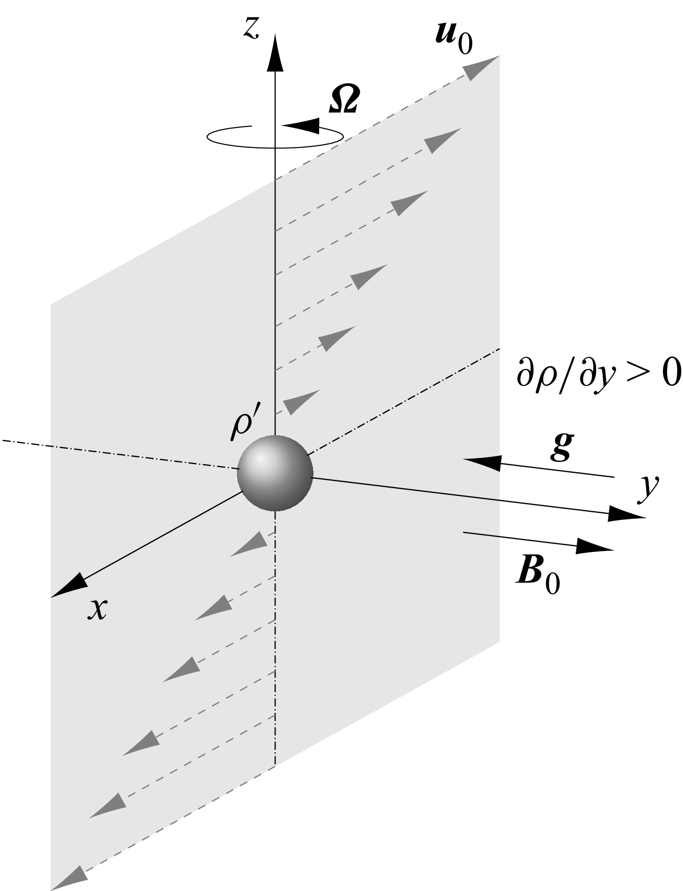


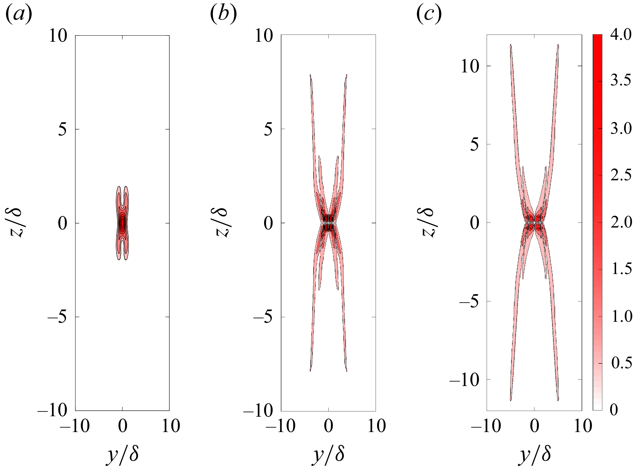


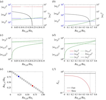


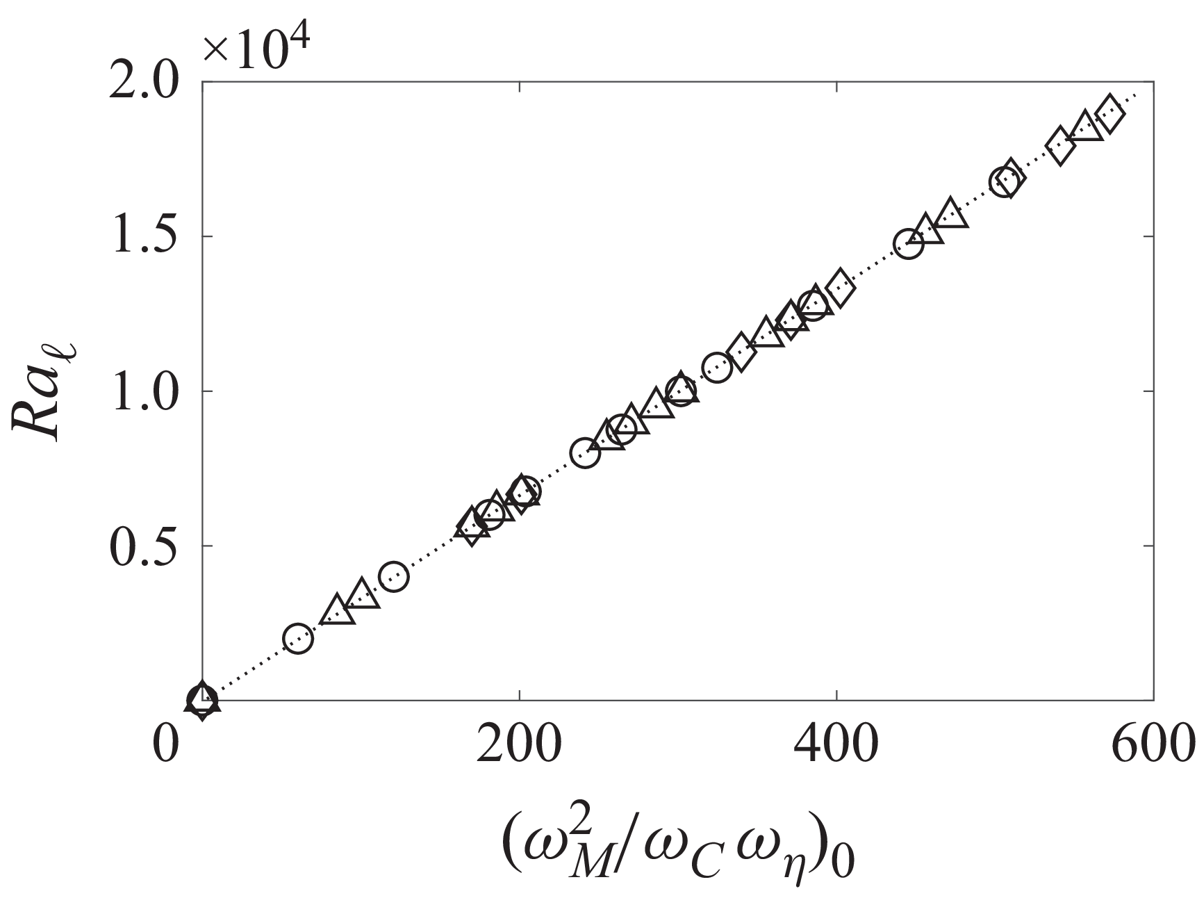


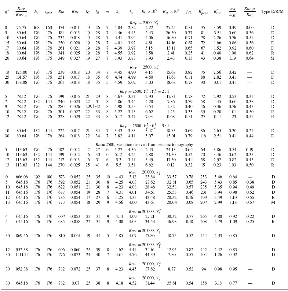


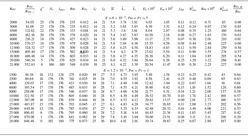


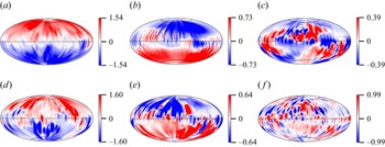


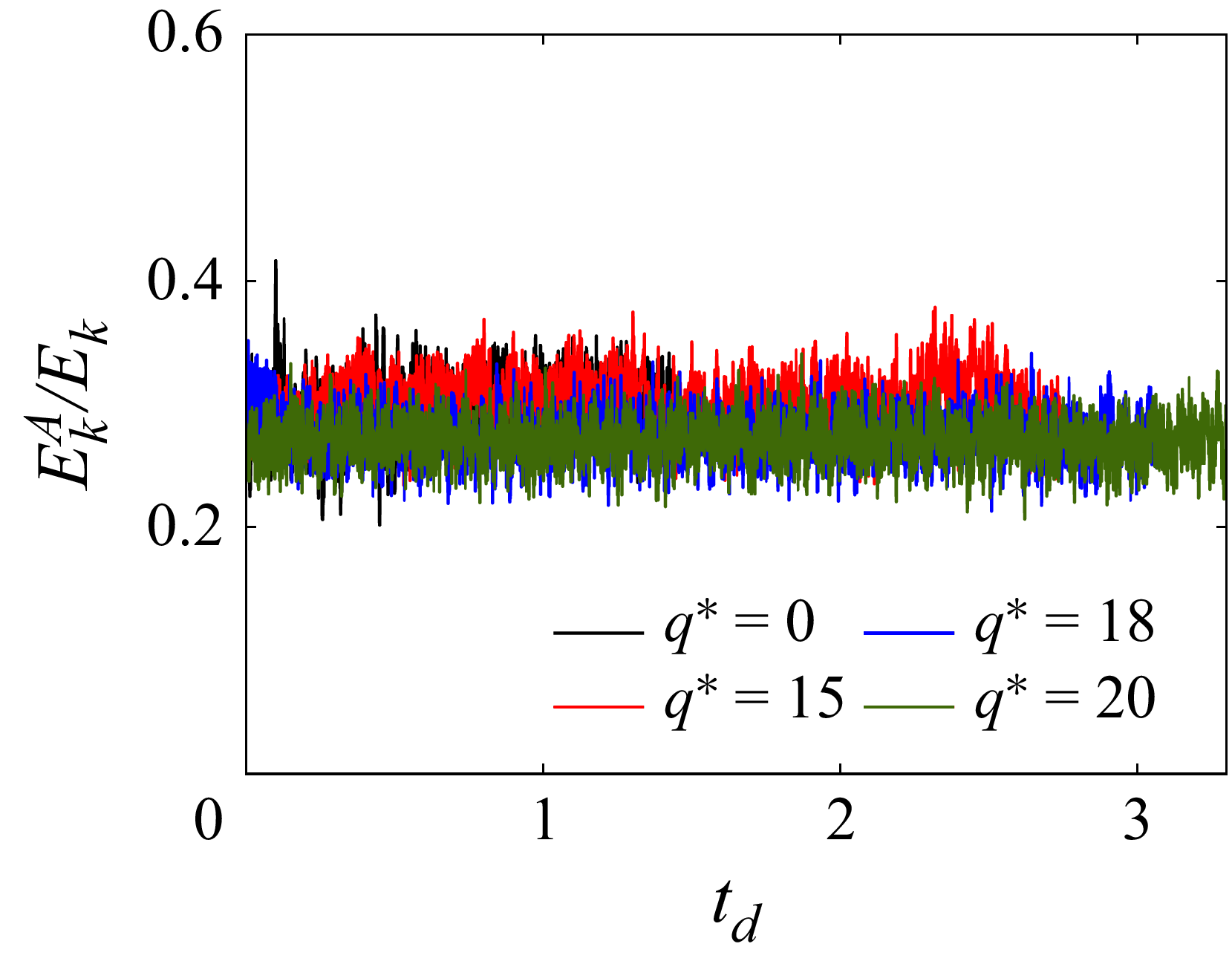


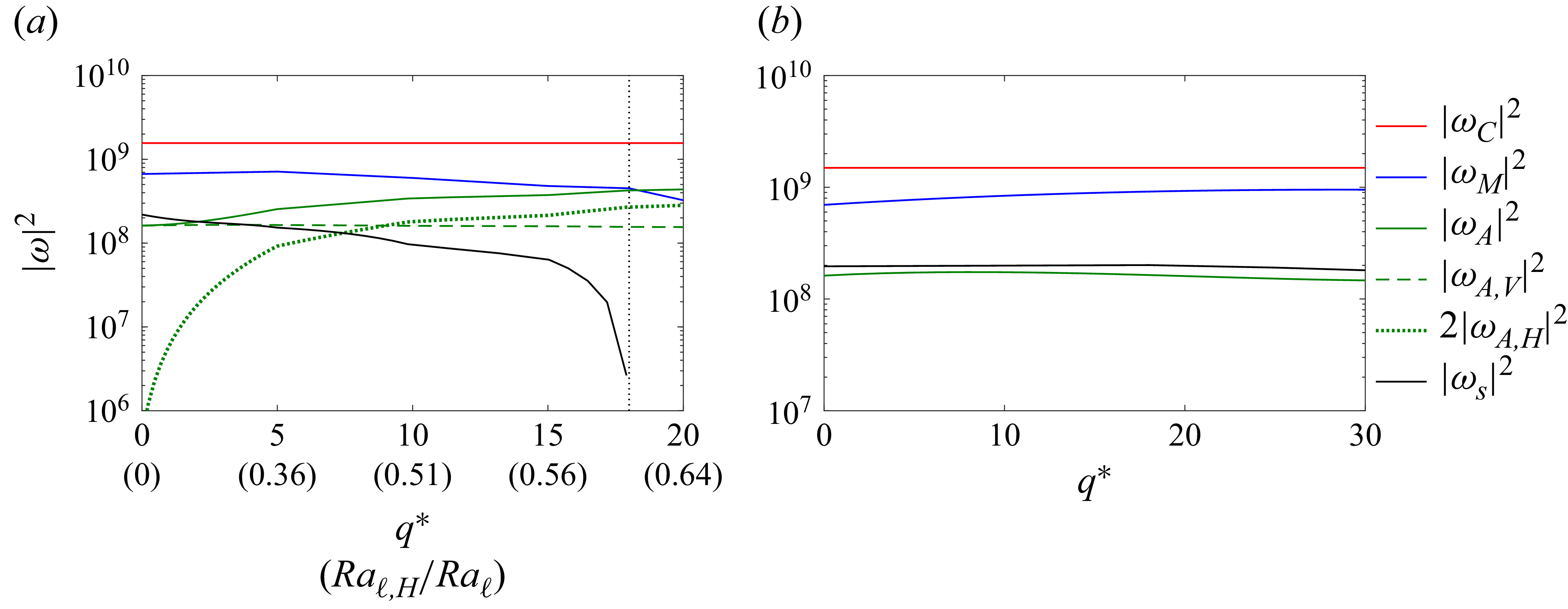


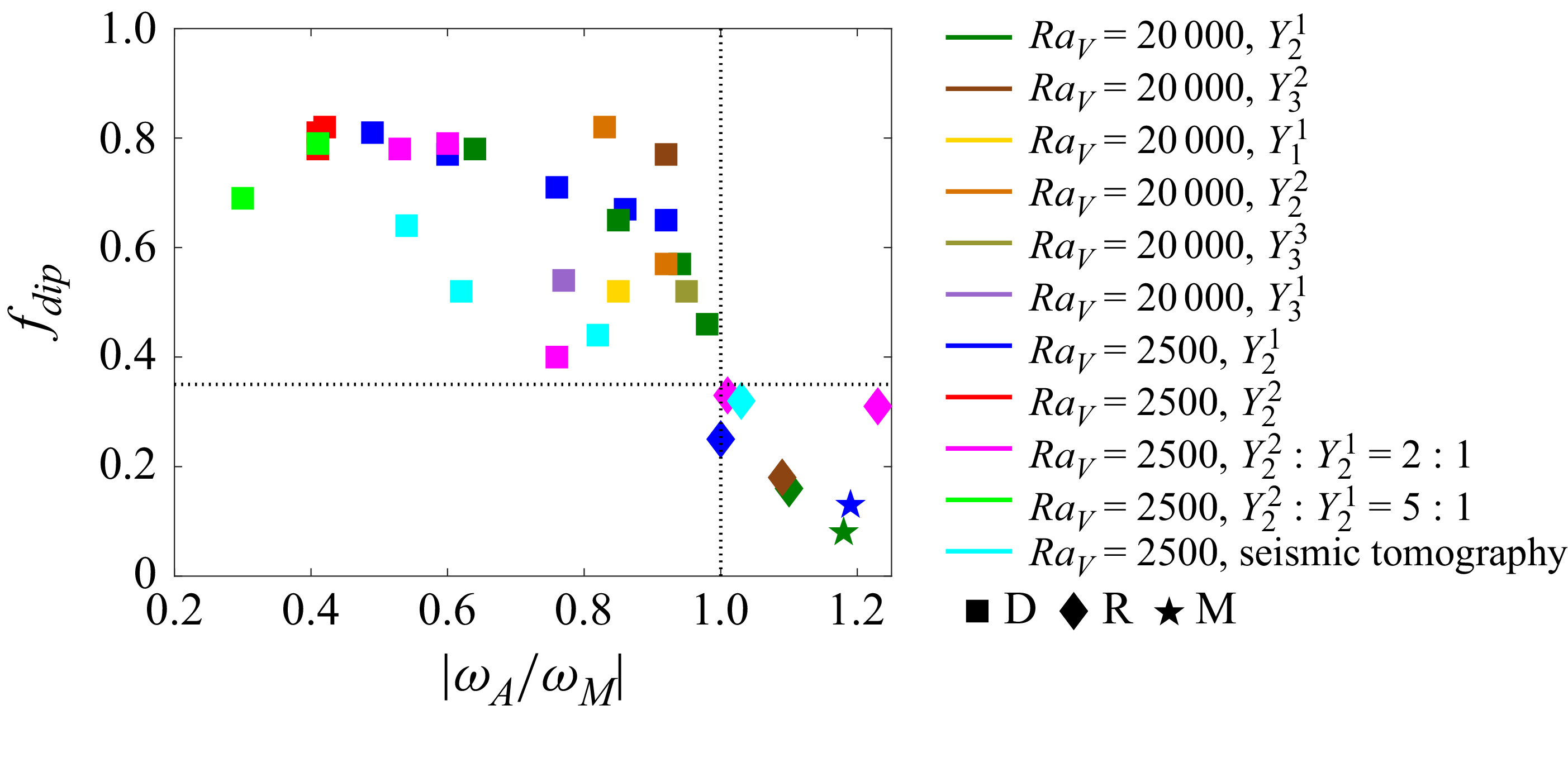


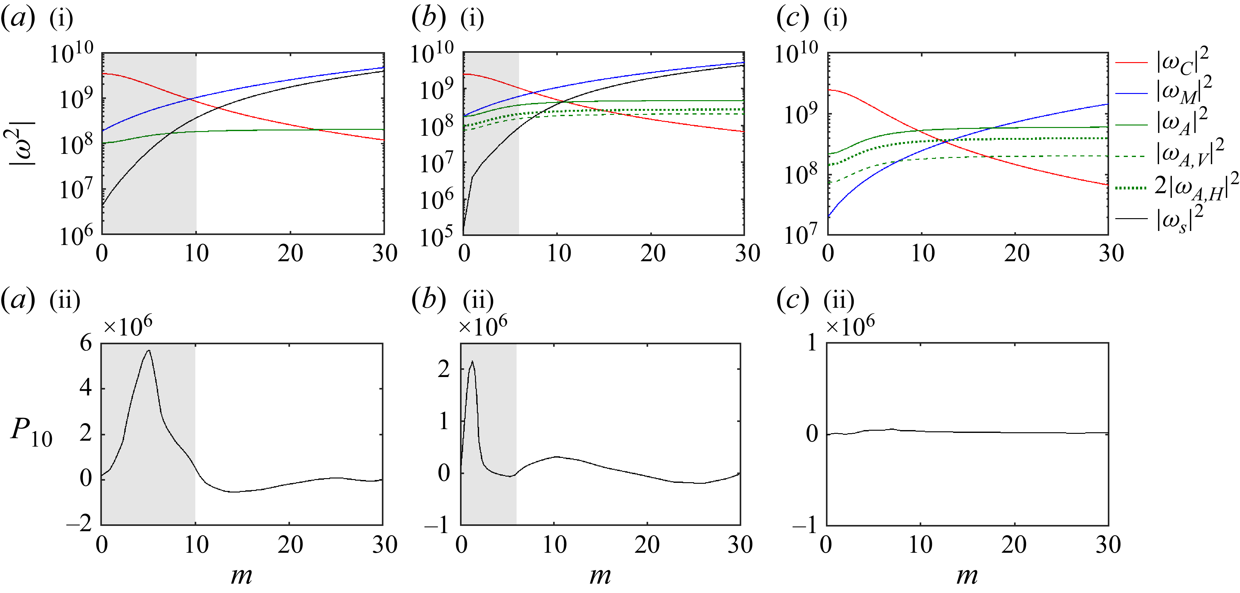


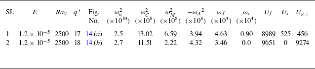


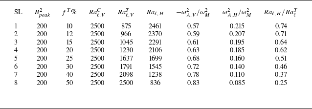


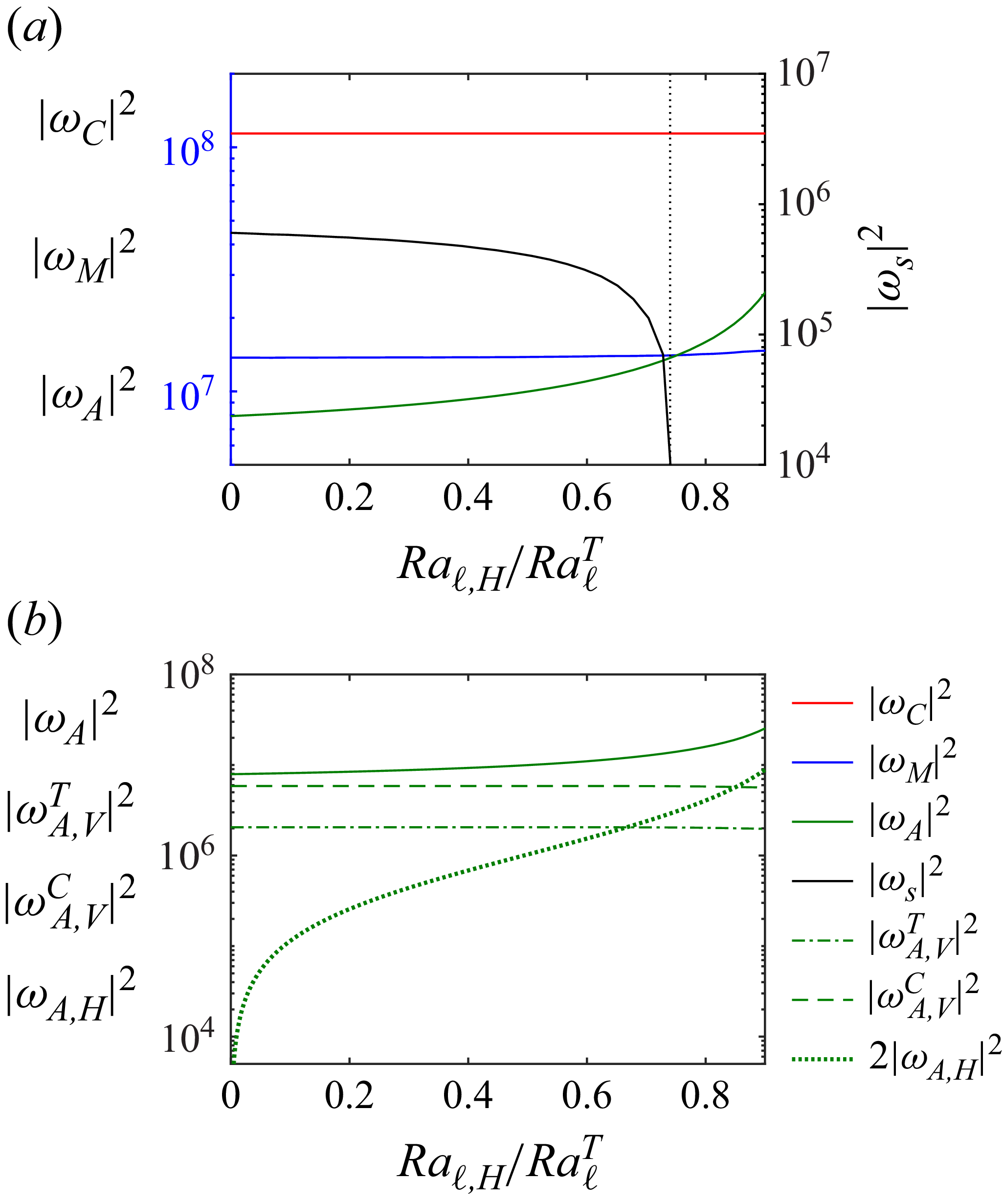


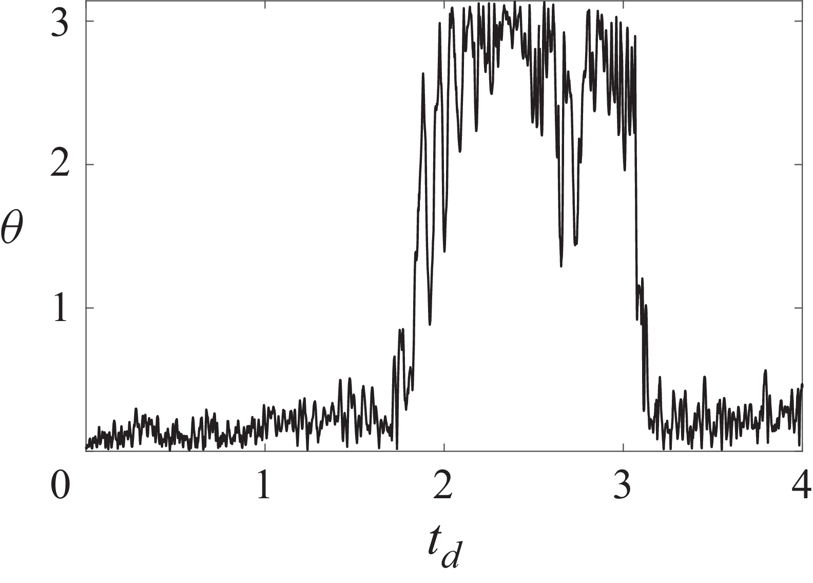


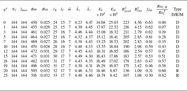


 Open access

