


1. Introduction
1.1. Background
Impact between liquid droplets and solid surfaces has been an important research topic for decades due to its ubiquity in the environment and technologies over a wide range of applications including spray-drying, aqueous jet-cleaning (Pergamalis Reference Pergamalis2002), jet-cutting, ink-jet printing, combustion, and deposition in pharmacology and agriculture (Bergeron et al. Reference Bergeron, Bonn, Jean and Vovelle2000). The liquid–solid impact can, however, also cause undesirable erosion problems as well. For example, water droplets are one of the greatest concerns in steam turbines of power plants (Smith Reference Smith1966), while raindrops are detrimental, or even fatal, to aircraft and missiles (Gohardani Reference Gohardani2011), and more recently, wind turbine blades (Hoksbergen, Akkerman & Baran Reference Hoksbergen, Akkerman and Baran2023). Impacts lead to removal of blade material, damage to aerofoil geometry and can even lead to component failure without an appropriate protective regime (Yang et al. Reference Yang, Tavner, Crabtree, Feng and Qiu2014). For these and other reasons, the detailed physics of liquid droplets impacting a solid surface has motivated research on this subject.
Analytical research on liquid droplet impact has, since at least
 $1920$
, sought to understand the impact loadings on the solid impact surface. This has shown that the unsteady pressure can be higher than the magnitude of the stagnation pressure corresponding to steady, incompressible flow. Among early works, a simplified one-dimensional water-hammer equation (Cook & Parsons Reference Cook and Parsons1928) has been widely used to approximate the peak pressure during impact, in the dimensional form, as
$1920$
, sought to understand the impact loadings on the solid impact surface. This has shown that the unsteady pressure can be higher than the magnitude of the stagnation pressure corresponding to steady, incompressible flow. Among early works, a simplified one-dimensional water-hammer equation (Cook & Parsons Reference Cook and Parsons1928) has been widely used to approximate the peak pressure during impact, in the dimensional form, as
 \begin{equation} P=\rho _0 C_0 U_0 \end{equation}
where
 $P$
denotes the surface pressure,
$P$
denotes the surface pressure,
 $\rho _0$
denotes the density,
$\rho _0$
denotes the density,
 $C_0$
denotes the sonic speed within the liquid,
$C_0$
denotes the sonic speed within the liquid,
 $U_0$
denotes the impact speed of the droplet and the subscript ‘
$U_0$
denotes the impact speed of the droplet and the subscript ‘
 $0$
’ refers to the original state of the liquid before impact. The high pressure of the water-hammer pressure wave comes from the compressibility of the liquid but the details of the unsteady flow, for example the temporal profile and the spatial features, including lateral lamella spreading and splashing, are neglected in the one-dimensional model. Hence the theory has limited applicability to most low-to-medium-speed droplet impact physics.
$0$
’ refers to the original state of the liquid before impact. The high pressure of the water-hammer pressure wave comes from the compressibility of the liquid but the details of the unsteady flow, for example the temporal profile and the spatial features, including lateral lamella spreading and splashing, are neglected in the one-dimensional model. Hence the theory has limited applicability to most low-to-medium-speed droplet impact physics.
1.2. Water-entry problem
In the rest of § 1, we present the literature results in dimensionless variables and expressions. Throughout this paper, variables are made dimensionless using
 $R_0$
,
$R_0$
,
 $U_0$
and
$U_0$
and
 $\rho _l$
, with
$\rho _l$
, with
 $R_0$
the droplet initial radius (in the case of wedge-shaped object, droplet radius is not applicable and an arbitrary length scale should be used instead),
$R_0$
the droplet initial radius (in the case of wedge-shaped object, droplet radius is not applicable and an arbitrary length scale should be used instead),
 $U_0$
the impact speed and
$U_0$
the impact speed and
 $\rho _l$
the liquid density; and lower-case letters denote dimensionless forms of corresponding upper-case variables, unless specified otherwise. Most of the progress in the field, however, has been made by the ‘opposite’, but intrinsically linked problem, of the water-entry of solid objects. Once again, from the
$\rho _l$
the liquid density; and lower-case letters denote dimensionless forms of corresponding upper-case variables, unless specified otherwise. Most of the progress in the field, however, has been made by the ‘opposite’, but intrinsically linked problem, of the water-entry of solid objects. Once again, from the
 $1920$
s, von Kármán (Reference von Kármán1929) in a pioneering paper introduced the problem of the vertical entry of a two-dimensional solid wedge with finite deadrise angle
$1920$
s, von Kármán (Reference von Kármán1929) in a pioneering paper introduced the problem of the vertical entry of a two-dimensional solid wedge with finite deadrise angle
 $\alpha$
(figure 1
a) in the context of predicting the impact force on a landing seaplane. He equated the impact force on an impacting two-dimensional object at time
$\alpha$
(figure 1
a) in the context of predicting the impact force on a landing seaplane. He equated the impact force on an impacting two-dimensional object at time
 $T$
to the force on a flat plate (Wilson Reference Wilson1989; Faltinsen & Wu Reference Faltinsen and Wu2001), of width
$T$
to the force on a flat plate (Wilson Reference Wilson1989; Faltinsen & Wu Reference Faltinsen and Wu2001), of width
 $2A(T)$
given by the intersection of the object and the undisturbed free surface (figure 1
a). For the latter, it is assumed that the fluid contained in a circular cylinder of diameter
$2A(T)$
given by the intersection of the object and the undisturbed free surface (figure 1
a). For the latter, it is assumed that the fluid contained in a circular cylinder of diameter
 $2A(T)$
is set into motion with the impact velocity
$2A(T)$
is set into motion with the impact velocity
 $U_0$
. The mass of this part of the fluid (for the water-entry problem, the cylinder is composed half of air and half of water, so a factor of
$U_0$
. The mass of this part of the fluid (for the water-entry problem, the cylinder is composed half of air and half of water, so a factor of
 $1/2$
is applied as the effect of the air phase is relatively negligible),
$1/2$
is applied as the effect of the air phase is relatively negligible),
 $M(T)=(1/2)\rho _l\pi A(T)^2$
, is referred to as ‘the apparent increase of the mass of the plate’ by von Kármán. This has momentum
$M(T)=(1/2)\rho _l\pi A(T)^2$
, is referred to as ‘the apparent increase of the mass of the plate’ by von Kármán. This has momentum
 $M(T)U_0$
. Hence the force to accelerate this part of the fluid (i.e. force on the plate) is the rate of change in momentum:
$M(T)U_0$
. Hence the force to accelerate this part of the fluid (i.e. force on the plate) is the rate of change in momentum:
 \begin{equation} F(T)=\frac {\text{d}}{\text{d}T}\big (M(T)U_0\big ). \end{equation}
In the dimensionless form, this force is
 \begin{equation} f(t)=\frac {1}{2}\frac {\text{d}}{\text{d}t}\big (\pi a(t)^2\big ). \end{equation}
For the original case of the solid wedge, the intersection radius
 $a(t)=t/\tan (\alpha )$
(figure 1
a); then, (1.3) leads to
$a(t)=t/\tan (\alpha )$
(figure 1
a); then, (1.3) leads to
 $f(t)=\pi a(t)/\tan (\alpha )$
. While for the case of a cylinder (Cointe & Armand Reference Cointe and Armand1987), the intersection radius
$f(t)=\pi a(t)/\tan (\alpha )$
. While for the case of a cylinder (Cointe & Armand Reference Cointe and Armand1987), the intersection radius
 $a(t)$
obeys the equation
$a(t)$
obeys the equation
 $(1-t)^2+a^2=1^2$
, which leads to
$(1-t)^2+a^2=1^2$
, which leads to
 $a(t)=\sqrt {2t-t^2}\approx \sqrt {2t}$
at small time; then, (1.3) leads to simply
$a(t)=\sqrt {2t-t^2}\approx \sqrt {2t}$
at small time; then, (1.3) leads to simply
 $\pi$
.
$\pi$
.

Figure 1. Sketch of the water-entry problem of a wedge with finite deadrise angle
 $\alpha$
(a) and its splashing, and the water-entry problem of object with small deadrise angle (b) assumed in Wagner’s water-entry solutions. The latter is related to the opposite problem of spherical droplet impact (c) which has deadrise angle
$\alpha$
(a) and its splashing, and the water-entry problem of object with small deadrise angle (b) assumed in Wagner’s water-entry solutions. The latter is related to the opposite problem of spherical droplet impact (c) which has deadrise angle
 $\alpha$
increases from
$\alpha$
increases from
 $0$
in time. Initial flow geometries are shown in light dashed lines.
$0$
in time. Initial flow geometries are shown in light dashed lines.
Wagner (Reference Wagner1932) subsequently refined von Kármán’s analysis by separating the impact and spreading (or splashing) problems, and introduced the concepts of an inner and outer region. For the outer region, the mathematical problem, to leading order, is reduced to that of a flat plate (for small deadrise angles, for example as shown in figure 1
b) of width
 $2a(t)$
entering into semi-infinite water. The derived leading-order solution of the outer problem comes from the unsteady Bernoulli pressure,
$2a(t)$
entering into semi-infinite water. The derived leading-order solution of the outer problem comes from the unsteady Bernoulli pressure,
 \begin{equation} p_{\textit{outer},1}(x,t)=\frac {1}{\sqrt {1-({x^2}/{a(t)^2)}}}\frac {\text{d}a(t)}{\text{d}t} \end{equation}
for coordinate
 $x$
on the solid surface, which has a positive integrable singularity at the plate edge
$x$
on the solid surface, which has a positive integrable singularity at the plate edge
 $a(t)$
due to the unsteady size change of the plate in time. For the inner region, Wagner used conformal mapping to transpose stagnation potential flow theory in the hodograph plane to the physical plane, assuming the kinematic condition that the solid surface meets the liquid free surface at the semiwidth of the equivalent flat plate
$a(t)$
due to the unsteady size change of the plate in time. For the inner region, Wagner used conformal mapping to transpose stagnation potential flow theory in the hodograph plane to the physical plane, assuming the kinematic condition that the solid surface meets the liquid free surface at the semiwidth of the equivalent flat plate
 $a(t)$
as a stagnation point. This leads to a solution in parametric form (as a result of the conformal mapping), for the inner region, known as the splash solution,
$a(t)$
as a stagnation point. This leads to a solution in parametric form (as a result of the conformal mapping), for the inner region, known as the splash solution,
 \begin{equation} p_{\textit{inner}}(\tau )=\frac {2\sqrt {-\tau }}{{\big (1+\sqrt {-\tau }\big )}^2} \end{equation}
where
 $\tau$
is the negative coordinate in the hodograph plane. The kinematic condition became known as the Wagner condition, which solves for the semiwidth of the plate to be
$\tau$
is the negative coordinate in the hodograph plane. The kinematic condition became known as the Wagner condition, which solves for the semiwidth of the plate to be
 $a(t)=\sqrt {3t}$
(for a spherically shaped object (Howison, Ockendon & Wilson Reference Howison, Ockendon and Wilson1991)). Here
$a(t)=\sqrt {3t}$
(for a spherically shaped object (Howison, Ockendon & Wilson Reference Howison, Ockendon and Wilson1991)). Here
 $a(t)=\sqrt {3t}$
is known as the ‘wet radius’ and its magnitude has shown excellent agreement with the experiments by Riboux & Gordillo (Reference Riboux and Gordillo2014). With the Wagner condition, Cointe & Armand (Reference Cointe and Armand1987) first produced a single composite solution by asymptotically matching the solutions from the two regions at the wet radius,
$a(t)=\sqrt {3t}$
is known as the ‘wet radius’ and its magnitude has shown excellent agreement with the experiments by Riboux & Gordillo (Reference Riboux and Gordillo2014). With the Wagner condition, Cointe & Armand (Reference Cointe and Armand1987) first produced a single composite solution by asymptotically matching the solutions from the two regions at the wet radius,
 \begin{equation} p_{\textit{composed}}(x,t)=\frac {1}{\epsilon }p_{\textit{outer},1}\left (\frac {x}{\epsilon },t\right )+\frac {1}{\epsilon ^2}p_{\textit{inner}}\left (\frac {x}{\epsilon ^3}-\frac {a}{\epsilon ^2},t\right ) - p_{overlap}(x,t) \end{equation}
where
 $\epsilon =\sqrt {t}$
is the asymptotic scale of the problem. By doing so, the singularity of the outer region at the wet radius is eliminated and the obtained pressure at all positions on the contact surface are of finite magnitudes. Interestingly, Wagner had also derived the second-order steady Bernoulli pressure, which is of a lower order of magnitude and is therefore often neglected, for the outer region,
$\epsilon =\sqrt {t}$
is the asymptotic scale of the problem. By doing so, the singularity of the outer region at the wet radius is eliminated and the obtained pressure at all positions on the contact surface are of finite magnitudes. Interestingly, Wagner had also derived the second-order steady Bernoulli pressure, which is of a lower order of magnitude and is therefore often neglected, for the outer region,
 \begin{equation} p_{\textit{outer},2}(x,t)=-\frac {x^2}{2\big ({a(t)}^2-x^2\big )}. \end{equation}
This steady component of the Bernoulli pressure contains a negative non-integrable singularity at the wet radius due to infinite flow ‘winding’, or turning, velocity. However, it was not integrated into the composite solutions by Cointe & Armand (Reference Cointe and Armand1987). The detailed mathematics of the asymptotic match and final explicit formulae can be seen in Wilson (Reference Wilson1989). The derived analytical solutions of the water-entry problem were further studied by Howison et al. (Reference Howison, Ockendon and Wilson1991) in the context of the reverse problem of water-exit, by Zhao & Faltinsen (Reference Zhao and Faltinsen1993) on penetrating objects of large deadrise angles, and later generalised by Korobkin (Reference Korobkin2004) to arbitrary deadrise angles.
1.3. Droplet impact problem
At the same time, Cointe (Reference Cointe1989) first commented that the water-entry problem of a solid object entering calm, flat water surface can be viewed as the opposite of a liquid object impacting onto a flat solid surface (figure 1
c). In this context, in particular, for solid objects of small deadrise angle, the solutions to the water-entry problem can be mapped to solutions for liquid droplet impact, since the geometry of a spherical droplet during ‘initial’ touching involves small contact angles. Since that publication, the two ‘opposite’ flows have been intrinsically linked together for analytical studies. Scolan (Reference Scolan2004) was the first work to extend the analysis into the axisymmetric case, and obtained the composed solution in an axisymmetric framework. When applying the solution to the droplet impact problem, Oliver (Reference Oliver2002) noticed that there exists an arbitrary shift of the inner solution in the hodograph plane, which characterises the radial stagnation point of the inner region in physical plane. Specifically for droplet impacts, the spreading or splashing lamella is ejected directly from the wet radius (Riboux & Gordillo Reference Riboux and Gordillo2016) (known as the ‘jet root’), and hence Oliver proposed a modification by shifting in non-dimensional distance by
 $6\delta /\pi$
for the inner solution along the surface towards the origin for droplet impact solution (see Appendix B), where
$6\delta /\pi$
for the inner solution along the surface towards the origin for droplet impact solution (see Appendix B), where
 $\delta$
is the asymptotic thickness of the jetting (see figure
$\delta$
is the asymptotic thickness of the jetting (see figure
 $9$
of Wagner (Reference Wagner1932)). Recently Negus et al. (Reference Negus, Moore, Oliver and Cimpeanu2021) obtained the axisymmetric liquid-droplet-impact-specific pressure solutions on the solid surface by composing the modified inner region pressure solution to the outer solution, and subsequently derived the impact force on the solid surface by integrating the impact pressure, in polar coordinates, on the solid surface.
$9$
of Wagner (Reference Wagner1932)). Recently Negus et al. (Reference Negus, Moore, Oliver and Cimpeanu2021) obtained the axisymmetric liquid-droplet-impact-specific pressure solutions on the solid surface by composing the modified inner region pressure solution to the outer solution, and subsequently derived the impact force on the solid surface by integrating the impact pressure, in polar coordinates, on the solid surface.

Figure 2. The ring erosion pattern (a) observed in experiments of droplet impact erosion studies are closely related to the ring-pressure pattern (b) on the solid surface upon droplet impact. (a) is from the experimental observations of Field (Reference Field1966). Panel (b) is from the numerical simulation developed in the present study, with parameters
 $R_0=1.1\ \textrm {mm}$
,
$R_0=1.1\ \textrm {mm}$
,
 $U_0=1.93\ \textrm {m s}^{-1}$
, kinematic viscosity of
$U_0=1.93\ \textrm {m s}^{-1}$
, kinematic viscosity of
 $20$
cSt and
$20$
cSt and
 $\textit{Re}=106$
at
$\textit{Re}=106$
at
 $\textit{TU}_0/R_0=2\times 10^{-1}$
, and all variables in the figure are presented in their dimensionless forms.
$\textit{TU}_0/R_0=2\times 10^{-1}$
, and all variables in the figure are presented in their dimensionless forms.
The original Wagner solutions have the inner and outer regions separated at the wet radius, where singularities exist. Since then, there have been studies to modify the Wagner solutions into a practical pressure solution. These suggest alternative spatial boundaries of the analytical solutions. Logvinovich (Reference Logvinovich1969), instead of composing solutions from the two regions, added the unsteady and steady components in the outer region. The combined solution presents a physically correct ring pressure pattern (figure 2) that has been widely observed in droplet impact erosion studies (Field, Lesser & Dear Reference Field, Lesser and Dear1985; Field Reference Field1966; Engel Reference Engel1955; Hancox & Brunton Reference Hancox and Brunton1966). Nevertheless, the solution also has a negative singularity at the wet radius, because the steady component is of a higher singularity order due to a quadratic effect. Logvinovich proposed this solution for
 $0\leqslant x\leqslant x_*(t)$
, where
$0\leqslant x\leqslant x_*(t)$
, where
 $x_*(t)\lt a(t)$
is the position that impact pressure reaches zero,
$x_*(t)\lt a(t)$
is the position that impact pressure reaches zero,
 \begin{equation} x_*(t)=\sqrt {2\big (\sqrt {1+2t}-1\big )}. \end{equation}
Using similar principles, Cointe & Armand (Reference Cointe and Armand1987) also proposed a solution by concatenating the outer solution (only the leading term of the unsteady Bernoulli) with the inner solution through a simple Heaviside function at
 $x_{s1}\lt a(t)$
, where the magnitude of the outer solution equals the maximum pressure of the inner solution. As a combination of the two ideas, Faltinsen & Wu (Reference Faltinsen and Wu2001) concatenated the outer solutions (both unsteady and steady Bernoulli) with the inner solution through a Heaviside function at
$x_{s1}\lt a(t)$
, where the magnitude of the outer solution equals the maximum pressure of the inner solution. As a combination of the two ideas, Faltinsen & Wu (Reference Faltinsen and Wu2001) concatenated the outer solutions (both unsteady and steady Bernoulli) with the inner solution through a Heaviside function at
 $x_{s1}$
(Faltinsen & Wu (Reference Faltinsen and Wu2001) use a different approach for, and hence find a different value of,
$x_{s1}$
(Faltinsen & Wu (Reference Faltinsen and Wu2001) use a different approach for, and hence find a different value of,
 $x_{s1}$
relative to Cointe & Armand (Reference Cointe and Armand1987)) or
$x_{s1}$
relative to Cointe & Armand (Reference Cointe and Armand1987)) or
 $x_{s2}$
, where
$x_{s2}$
, where
 $x_{s1} \leqslant x_{s2}\lt a(t)$
are the two points where the magnitude of the (combined) outer solution equals the maximum pressure of the inner solution due to the ring-pressure pattern. However, with this approach, it is difficult to algebraically derive an explicit expression for the two points
$x_{s1} \leqslant x_{s2}\lt a(t)$
are the two points where the magnitude of the (combined) outer solution equals the maximum pressure of the inner solution due to the ring-pressure pattern. However, with this approach, it is difficult to algebraically derive an explicit expression for the two points
 $x_{s1}$
and
$x_{s1}$
and
 $x_{s2}$
, and therefore these were concatenated numerically in practice.
$x_{s2}$
, and therefore these were concatenated numerically in practice.
Alternative progress in liquid droplet impact studies has been made by using classical potential flow theories and other approaches. Riboux & Gordillo have performed the hydrodynamic approach, assuming the droplet to be an ideal fluid field (Riboux & Gordillo Reference Riboux and Gordillo2014, Reference Riboux and Gordillo2015, Reference Riboux and Gordillo2016; Gordillo, Riboux & Quintero Reference Gordillo, Sun and Cheng2018, Reference Gordillo, Riboux and Quintero2019). A series of analytical solutions have been derived focusing on spreading and splashing behaviours, including lamella ejection, jet speed, splashing criteria, dewetting and lubrication effects. In particular, Gordillo et al. (Reference Gordillo, Riboux and Quintero2019) employed Lamb’s hydrodynamic model of the flat disk in an infinite mass of liquid (Lamb Reference Lamb1916) to solve the flow velocities on the solid surface. Other studies found that the impact force from this inviscid potential flow theory captures the inertial-force scalings observed in experiments at early times (Cheng, Sun & Gordillo Reference Cheng, Sun and Gordillo2022) and the low-viscosity scenario (Sanjay et al. Reference Sanjay, Zhang, Lv and Lohse2025), but does not include viscous damping which is shown to be important for the later force decay in the spreading regimes (Roisman Reference Roisman2009; Roisman, Berberović & Tropea Reference Roisman, Berberović and Tropea2009; García-Geijo et al. Reference García-Geijo, Riboux and Gordillo2020; Sanjay et al. Reference Sanjay, Zhang, Lv and Lohse2025; Sanjay & Lohse Reference Sanjay and Lohse2025). The dependence of maximum impact force on the Reynolds,
 $\textit{Re}$
(Cheng et al. Reference Cheng, Sun and Gordillo2022), Weber,
$\textit{Re}$
(Cheng et al. Reference Cheng, Sun and Gordillo2022), Weber,
 $\textit{We}$
(Zhang et al. Reference Zhang, Sanjay, Shi, Zhao, Lv, Feng and Lohse2022) and Ohnesorge
$\textit{We}$
(Zhang et al. Reference Zhang, Sanjay, Shi, Zhao, Lv, Feng and Lohse2022) and Ohnesorge
 $\textit{Oh}$
(Sanjay et al. Reference Sanjay, Zhang, Lv and Lohse2025; Sanjay & Lohse Reference Sanjay and Lohse2025) numbers was investigated. Regarding the late-time spreading and deposition regimes, Eggers et al. (Reference Eggers, Fontelos, Josserand and Zaleski2010) used mass and momentum conservation to analytically predict the temporal expanding radius of the lamella. The dependence of maximum spreading radius on
$\textit{Oh}$
(Sanjay et al. Reference Sanjay, Zhang, Lv and Lohse2025; Sanjay & Lohse Reference Sanjay and Lohse2025) numbers was investigated. Regarding the late-time spreading and deposition regimes, Eggers et al. (Reference Eggers, Fontelos, Josserand and Zaleski2010) used mass and momentum conservation to analytically predict the temporal expanding radius of the lamella. The dependence of maximum spreading radius on
 $\textit{We}$
and
$\textit{We}$
and
 $\textit{Oh}$
was explored in Sanjay & Lohse (Reference Sanjay and Lohse2025); García-Geijo et al. (Reference García-Geijo, Riboux and Gordillo2020). In other topics, Josserand & Zaleski (Reference Josserand and Zaleski2003) studied lamella ejection and the transition between splashing and deposition for impacting droplets with the presence of a liquid film. Thoroddsen et al. (Reference Thoroddsen, Etoh, Takehara, Ootsuka and Hatsuki2005) and García-Geijo et al. (Reference García-Geijo, Riboux and Gordillo2024) investigated air-bubble entrapment at initial droplet touching. Besides, there is an interesting observation of a ‘second peak’ in the impact force as the droplet jumps off hydrophobic surfaces (Zhang et al. Reference Zhang, Sanjay, Shi, Zhao, Lv, Feng and Lohse2022; Sanjay et al. Reference Sanjay, Zhang, Lv and Lohse2025). Readers are referred to Josserand & Thoroddsen (Reference Josserand and Thoroddsen2016) for a comprehensive review of recent progresses in droplet impact studies, and, in particular, Cheng et al. (Reference Cheng, Sun and Gordillo2022) for impact force studies. However, this body of the literature does not lead to analytical models of impact pressure on the solid surface, which is the focus of the present study.
$\textit{Oh}$
was explored in Sanjay & Lohse (Reference Sanjay and Lohse2025); García-Geijo et al. (Reference García-Geijo, Riboux and Gordillo2020). In other topics, Josserand & Zaleski (Reference Josserand and Zaleski2003) studied lamella ejection and the transition between splashing and deposition for impacting droplets with the presence of a liquid film. Thoroddsen et al. (Reference Thoroddsen, Etoh, Takehara, Ootsuka and Hatsuki2005) and García-Geijo et al. (Reference García-Geijo, Riboux and Gordillo2024) investigated air-bubble entrapment at initial droplet touching. Besides, there is an interesting observation of a ‘second peak’ in the impact force as the droplet jumps off hydrophobic surfaces (Zhang et al. Reference Zhang, Sanjay, Shi, Zhao, Lv, Feng and Lohse2022; Sanjay et al. Reference Sanjay, Zhang, Lv and Lohse2025). Readers are referred to Josserand & Thoroddsen (Reference Josserand and Thoroddsen2016) for a comprehensive review of recent progresses in droplet impact studies, and, in particular, Cheng et al. (Reference Cheng, Sun and Gordillo2022) for impact force studies. However, this body of the literature does not lead to analytical models of impact pressure on the solid surface, which is the focus of the present study.
For work that does address impact pressure, Philippi, Lagrée & Antkowiak (Reference Philippi, Lagrée and Antkowiak2016) has developed a self-similar theory of the liquid flow field evolution at early time, with the surface pressure given by
 \begin{equation} \hat {p}(\xi ,\eta =0)=\frac {3}{\pi \sqrt {3-\xi ^2}} \end{equation}
where
 $\hat {p}=p/\sqrt {t}$
,
$\hat {p}=p/\sqrt {t}$
,
 $\xi =r/\sqrt {t}$
and
$\xi =r/\sqrt {t}$
and
 $\eta =z/\sqrt {t}$
are the pressure and spatial variables, respectively, in self-similar space. This work demonstrates the analogy between Wagner’s water-entry theory (Wagner Reference Wagner1932), Lamb’s flat disk model (Lamb Reference Lamb1916) and the droplet impact problem. Philippi et al.'s solution of the liquid flow field, particularly of the impact pressure on the solid surface, compares well with numerical simulations at early time, and hence the self-similar dynamics are verified on the solid surface. Interestingly, we note that the impact pressure solution (1.9) on the solid surface derived from the self-similar setting turns out to be exactly the same as the unsteady Bernoulli solution
$\eta =z/\sqrt {t}$
are the pressure and spatial variables, respectively, in self-similar space. This work demonstrates the analogy between Wagner’s water-entry theory (Wagner Reference Wagner1932), Lamb’s flat disk model (Lamb Reference Lamb1916) and the droplet impact problem. Philippi et al.'s solution of the liquid flow field, particularly of the impact pressure on the solid surface, compares well with numerical simulations at early time, and hence the self-similar dynamics are verified on the solid surface. Interestingly, we note that the impact pressure solution (1.9) on the solid surface derived from the self-similar setting turns out to be exactly the same as the unsteady Bernoulli solution
 $p_{\textit{outer},1}(x,t)$
of (1.4) developed by Wagner (Reference Wagner1932), and thereby also contains a positive singularity at the wet radius.
$p_{\textit{outer},1}(x,t)$
of (1.4) developed by Wagner (Reference Wagner1932), and thereby also contains a positive singularity at the wet radius.
Despite recent progress in analytical descriptions of the flow dynamics upon liquid droplet impact, analytical solutions that characterise the complete, or at least most of the evolution of the flow on the impacted solid surface, still do not exist. All the above-mentioned literature that has analytical descriptions of the impact pressure on the impact surface is summarised in table 1 (in order of publication date), including their solution components and respective spatial boundaries. Generally speaking, the existing liquid–solid impact solutions are composed of steady and/or unsteady components which, however, suffer from singularities at the wet radius, especially for the steady component which is non-integrable. Some of the other solutions are composed of the splash solution of the inner region which, however, suffer from the implicit form of the parametric equations. This makes the final solutions complex and costly to apply in engineering applications. Besides, as far as we know, none of the above studies has their solutions applicable to non-normal impact angles. Finally, the existing analytical impact pressure solutions are incapable of reproducing an important physical feature which is observed in droplet impact erosion studies (Hancox & Brunton Reference Hancox and Brunton1966; Field et al. Reference Field, Lesser and Dear1985), namely the transition from the ring pressure pattern at early time to the centred maximum of pressure at intermediate time. It is therefore the aim of the current study to develop an analytical model of the liquid–solid impact problem that could fill the above gaps in the literature. Compared with more widely employed experimental and numerical simulation approaches, analytical models provide deep physical insights and are convenient to apply in engineering applications. These benefits make analytical models useful and uniquely important in the development of the field. There are five objectives in this work, as follows.
Table 1. Publications using analytical methods to study liquid–solid impact pressure, in ascending order of publication date. The three rightmost major column headings show which publications consider the terms for unsteady Bernoulli flow, steady Bernoulli flow and for splash solution. Minor column headings show whether a publication considers the spatial boundaries of the four features
 $x_{s1}$
,
$x_{s1}$
,
 $x_{s2}$
,
$x_{s2}$
,
 $x_*$
and
$x_*$
and
 $x=a$
, or
$x=a$
, or
 $r_{s1}$
,
$r_{s1}$
,
 $r_{s2}$
,
$r_{s2}$
,
 $r_*$
and
$r_*$
and
 $r=a$
, depending upon whether the geometry considered is two-dimensional planar, denoted by ‘
$r=a$
, depending upon whether the geometry considered is two-dimensional planar, denoted by ‘
 $2$
-D’, or is axisymmetric, denoted by ‘axi’. For the splash solution, we indicate whether the solution has been shifted in space by
$2$
-D’, or is axisymmetric, denoted by ‘axi’. For the splash solution, we indicate whether the solution has been shifted in space by
 $6\delta /\pi$
.
$6\delta /\pi$
.

-
(i) To develop a potential flow model for general liquid–solid impact that contains both the steady and unsteady characterisations of the flow field’s evolution as a function of time and space, and with arbitrary incidence. To achieve this, the reasons behind the singularities need to be analysed and hence resolved with physical interpretations.
-
(ii) To apply the developed model specifically to the droplet impact problem to obtain solutions for the impact pressure and force in closed form.
-
(iii) To analytically capture the physical ring pressure pattern on the impact surface at early time, and characterise the shifts in the stagnation pattern temporally and spatially at intermediate time. To achieve this, long-time validation of the developed analytical solution that covers both the early and intermediate phases of droplet impact is required.
-
(iv) To develop a high-fidelity numerical simulation to provide numerical comparisons with, and validations of, the developed analytical solutions, including both temporal and spatial pressure profiles and the impact force.
-
(v) Based on the developed droplet impact solution, to provide more accurate guidance on impact erosion studies with interpretation of physics.
This paper is organised as follows. Section 2 proposes a novel analytical model for general liquid–solid impacts. Section 3 applies the analytical model to the liquid droplet impact problem and obtains the impact pressure and force solution on the solid surface. Section 4 develops a validated high-fidelity numerical simulation that provides numerical comparisons with, and validations of, the derived analytical liquid droplet impact solutions on the solid surface. Comments on the validities of the analytical solution and inviscid features of the flow field are made in § 5. Finally, § 6 summarises the main results of the present study, and concludes with its perspectives.
2. Model
2.1. Mathematical description of the problem
2.1.1. Theoretical framework
Philippi et al. (Reference Philippi, Lagrée and Antkowiak2016) ‘… put forward in particular a so-called ‘Lamb analogy’ mirroring the flow within the impacting droplet with the one induced with a flat rising expanding disk…’ (see figure 3). The equations describing the impact-induced flow within the droplet have both steady and unsteady terms but some research analyses only the latter due to its higher order of magnitude at early times (Riboux & Gordillo Reference Riboux and Gordillo2014; Philippi et al. Reference Philippi, Lagrée and Antkowiak2016; Negus et al. Reference Negus, Moore, Oliver and Cimpeanu2021). However, Lamb’s original problem (Lamb Reference Lamb1916) (below called ‘steady disk’ (SD)) describes the steady flow around a flat rising disk, which does not have an unsteady component. Philippi et al. showed that by transposing Lamb’s steady solution into rescaled lengths of
 $l/\sqrt {t}$
, where
$l/\sqrt {t}$
, where
 $l$
represents any length variable and time
$l$
represents any length variable and time
 $t$
acts as a normalisation parameter, Lamb’s solution becomes a quasi-time-dependent expression and is an analogue to the impact-induced flow in self-similar space (below called ‘self-similar disk’ (SSD)). We build on this, but here we hypothesise that the disk radius
$t$
acts as a normalisation parameter, Lamb’s solution becomes a quasi-time-dependent expression and is an analogue to the impact-induced flow in self-similar space (below called ‘self-similar disk’ (SSD)). We build on this, but here we hypothesise that the disk radius
 $a$
in Lamb’s original problem is now a function of
$a$
in Lamb’s original problem is now a function of
 $t$
, and we will explore the full unsteady potential flow of this flat, rising, expanding disk including both steady and unsteady components (below called ‘unsteady disk’ (UD)). The UD framework has a fundamental difference from the SSD, as we shall see; and we propose the former UD as being a better framework to make an analogy with the droplet impact problem.
$t$
, and we will explore the full unsteady potential flow of this flat, rising, expanding disk including both steady and unsteady components (below called ‘unsteady disk’ (UD)). The UD framework has a fundamental difference from the SSD, as we shall see; and we propose the former UD as being a better framework to make an analogy with the droplet impact problem.

Figure 3. The problem of liquid droplet impact (downwards at velocity
 $u_0$
) onto a solid surface (a) has been found to have analogies with the problem of a rising expanding circular disk (moving upwards at velocity
$u_0$
) onto a solid surface (a) has been found to have analogies with the problem of a rising expanding circular disk (moving upwards at velocity
 $u_0$
) in an infinite mass of liquid (b). The yellow straight arrows in (a) denote the spreading of the wet radius (or contact line before lamella ejection), while the yellow curved arrows in (b) denote the winding motions of the liquid flows around the wet radius of the disk and the blue arrows denote the radial expansion of the disk with the wet radius. Figures are made after Philippi et al. (Reference Philippi, Lagrée and Antkowiak2016).
$u_0$
) in an infinite mass of liquid (b). The yellow straight arrows in (a) denote the spreading of the wet radius (or contact line before lamella ejection), while the yellow curved arrows in (b) denote the winding motions of the liquid flows around the wet radius of the disk and the blue arrows denote the radial expansion of the disk with the wet radius. Figures are made after Philippi et al. (Reference Philippi, Lagrée and Antkowiak2016).
2.1.2. Governing equations
Lamb’s mathematical problem, the SD framework, relates to the motion of a thin circular disk of radius
 $a$
with constant velocity
$a$
with constant velocity
 $\boldsymbol{u_0}$
normal to its plane in an infinite mass of liquid. In the inertial frame of reference moving at velocity
$\boldsymbol{u_0}$
normal to its plane in an infinite mass of liquid. In the inertial frame of reference moving at velocity
 $\boldsymbol{u_0}$
, the origin is taken at the centre of the disk for all time
$\boldsymbol{u_0}$
, the origin is taken at the centre of the disk for all time
 $t\geqslant 0$
. Lamb described the flow as an incompressible and inviscid axisymmetric ideal fluid field with the far field at rest (hence irrotational), so we can define a velocity potential
$t\geqslant 0$
. Lamb described the flow as an incompressible and inviscid axisymmetric ideal fluid field with the far field at rest (hence irrotational), so we can define a velocity potential
 $\phi (r,z)$
:
$\phi (r,z)$
:
 \begin{equation} \boldsymbol{u}(r,z)=\boldsymbol{\nabla }\phi (r,z). \end{equation}
By the mass conservation law,
 $\phi (r,z)$
satisfies the Laplacian equation, written in cylindrical coordinates,
$\phi (r,z)$
satisfies the Laplacian equation, written in cylindrical coordinates,
 \begin{equation} \boldsymbol{\nabla} ^2\phi =\frac {1}{r} \frac {\partial }{\partial r} \left ( r \frac {\partial \phi }{\partial r} \right ) + \frac {\partial ^2 \phi }{\partial z^2}=0 \end{equation}
and Bernoulli’s conservation equation for mechanical energy in an isentropic flow with negligible change in gravitational potential energy, everywhere in the liquid is
 \begin{equation} \frac {1}{2} |\boldsymbol{\nabla }\phi |^2 + \frac {p}{\rho } = \rm const. \end{equation}
where the dimensionless density
 $\rho$
is
$\rho$
is
 $1$
. The ideal fluid field in a designated control volume satisfies three boundary conditions, namely
$1$
. The ideal fluid field in a designated control volume satisfies three boundary conditions, namely
 \begin{equation} \frac {\partial \phi }{\partial z}(r,0)=1 \quad \text{for} \quad r \leqslant a \end{equation}
due to non-permeability at the disk surface
 $z=0$
; and
$z=0$
; and
 \begin{equation} \phi (r,0)=0 \quad \text{for} \quad r \gt a \end{equation}
and
 \begin{equation} \boldsymbol{\nabla }\phi (r,z)\rightarrow 0 \quad \text{as} \quad r^2+z^2 \rightarrow \infty \end{equation}
because the velocity field is undisturbed far from the disk’s surface.
For the model UD framework, studied here, however, we additionally assume the disk is also expanding in radius
 $a(t)$
in time, so the equations are unsteady. With the new time-dependent velocity potential
$a(t)$
in time, so the equations are unsteady. With the new time-dependent velocity potential
 $\phi (r,z,t)$
:
$\phi (r,z,t)$
:
 \begin{equation} \boldsymbol{u}(r,z,t)=\boldsymbol{\nabla }\phi (r,z,t). \end{equation}
The set of (2.2), (2.3) subject to boundary conditions (2.4)–(2.6) now read, respectively, as follows:
 \begin{equation} \boldsymbol{\nabla} ^2\phi =\frac {1}{r} \frac {\partial }{\partial r} \left ( r \frac {\partial \phi }{\partial r} \right ) + \frac {\partial ^2 \phi }{\partial z^2}=0, \end{equation}
 \begin{equation} \frac {\partial \phi }{\partial t} + \frac {1}{2} |\boldsymbol{\nabla }\phi |^2 + \frac {p}{\rho } = b(t), \end{equation}
where
 $b(t)$
is a function of time only, and three boundary conditions,
$b(t)$
is a function of time only, and three boundary conditions,
 \begin{equation} \frac {\partial \phi }{\partial z}(r,0,t)=1 \quad \text{for} \quad r \leqslant a(t), t \geqslant 0, \end{equation}
 \begin{equation} \phi (r,0,t)=0 \quad \text{for} \quad r \gt a(t), t \geqslant 0, \end{equation}
 \begin{equation} \boldsymbol{\nabla }\phi (r,z,t)\rightarrow 0 \quad \text{as} \quad r^2+z^2 \rightarrow \infty , t \geqslant 0. \end{equation}
Figure 4 presents the geometries of the SD and UD models, and summarises corresponding governing equations.

Figure 4. The control volume of the theoretical frameworks for a SD (a) and an UD (
 $a(t)$
) (b), including problem geometries, boundary conditions and the governing equations.
$a(t)$
) (b), including problem geometries, boundary conditions and the governing equations.
2.1.3. Analogy with an expanding water-entry problem

Figure 5. The two-dimensional potential flow theory for flow over a thin plate (a) in
 $\hat {z}$
plane can be derived from the potential flow past a cylinder (b) in
$\hat {z}$
plane can be derived from the potential flow past a cylinder (b) in
 $\hat {\zeta }$
plane using conformal mappings. By the same principle, the proposed expanding water-entry problem for an expanding cylinder (d) in (vertically flipped)
$\hat {\zeta }$
plane using conformal mappings. By the same principle, the proposed expanding water-entry problem for an expanding cylinder (d) in (vertically flipped)
 $\hat {\zeta }$
plane can be mapped to the
$\hat {\zeta }$
plane can be mapped to the
 $\hat {z}$
plane (c). The dashed line in (d) denotes the free water surface in the water-entry problem (see figures 1
a and 1
b) with the intersections with the object marked by yellow crosses. The dashed line and yellow crosses are then mapped to (c) as the droplet free interface and intersections with the solid surface, respectively. Flow streamlines in (c) and (d) are continued in transparency beyond liquid free interface for comparison with (a) and (b).
$\hat {z}$
plane (c). The dashed line in (d) denotes the free water surface in the water-entry problem (see figures 1
a and 1
b) with the intersections with the object marked by yellow crosses. The dashed line and yellow crosses are then mapped to (c) as the droplet free interface and intersections with the solid surface, respectively. Flow streamlines in (c) and (d) are continued in transparency beyond liquid free interface for comparison with (a) and (b).
When observing a side view of the disk, the rising thin flat disk in an infinite depth of flow field (in the frame of reference moving with the disk’s centre) is nothing other than the well-known flow around a thin flat plate with incidence (at an angle of attack
 $\pi /2$
) in two-dimensional potential flow theory (see figure 5
a). The solution to this classic mathematical problem can be obtained by conformal mappings from the known potential flow past a cylinder (figure 5
b). In particular, the Joukovskii transformation is a conformal mapping that can achieve this goal. We use the ‘hat’ symbol to denote flow quantities in two-dimensional potential flow theory,
$\pi /2$
) in two-dimensional potential flow theory (see figure 5
a). The solution to this classic mathematical problem can be obtained by conformal mappings from the known potential flow past a cylinder (figure 5
b). In particular, the Joukovskii transformation is a conformal mapping that can achieve this goal. We use the ‘hat’ symbol to denote flow quantities in two-dimensional potential flow theory,
 \begin{equation} \hat {z}= \frac {1}{2} \left ( \hat {\zeta } + \frac {\hat {a}^2}{\hat {\zeta }} \right ) \end{equation}
where
 $\hat {z}$
is the complex variable in the two-dimensional plane of the plate with length
$\hat {z}$
is the complex variable in the two-dimensional plane of the plate with length
 $2\hat {a}$
, and
$2\hat {a}$
, and
 $\hat {\zeta }$
is the complex variable in the two-dimensional plane of the cylinder with radius
$\hat {\zeta }$
is the complex variable in the two-dimensional plane of the cylinder with radius
 $\hat {a}$
.
$\hat {a}$
.
By this principle, the Joukovskii transformation (2.13) relates (the side view of) the proposed expanding UD framework (figure 5
c) in the current work to an ‘expanding water-entry problem’, as in figure 5(d) with flipped vertical direction relative to figure 5(c). The latter describes a cylinder of expanding radius
 $a(t)$
that moves towards initially calm water. We note the analogy, as well as the difference, of this ‘expanding water-entry problem’ to the well-known water-entry problem (Wagner Reference Wagner1932; Wilson Reference Wilson1989) where the solid object has a fixed radius. In the considered analogy (i.e. expanding water-entry problem) of figure 5(d), the flow field behaves as that in figure 5(b). However, due to the presence of the water surface (denoted as dashed line in figure 5
d), only the bottom part of the flow (denoted as non-transparent streamlines) is valid in the expanding water-entry problem. These streamlines intersect the object, namely the expanding cylinder, at the yellow crosses (Wagner Reference Wagner1932; Wilson Reference Wilson1989). Now, if we apply the Joukovskii transformation (2.13) to the expanding water-entry geometry of figure 5(d), we obtain the potential flow around a thin flat plate in the
$a(t)$
that moves towards initially calm water. We note the analogy, as well as the difference, of this ‘expanding water-entry problem’ to the well-known water-entry problem (Wagner Reference Wagner1932; Wilson Reference Wilson1989) where the solid object has a fixed radius. In the considered analogy (i.e. expanding water-entry problem) of figure 5(d), the flow field behaves as that in figure 5(b). However, due to the presence of the water surface (denoted as dashed line in figure 5
d), only the bottom part of the flow (denoted as non-transparent streamlines) is valid in the expanding water-entry problem. These streamlines intersect the object, namely the expanding cylinder, at the yellow crosses (Wagner Reference Wagner1932; Wilson Reference Wilson1989). Now, if we apply the Joukovskii transformation (2.13) to the expanding water-entry geometry of figure 5(d), we obtain the potential flow around a thin flat plate in the
 $\hat {z}$
-plane in figure 5(c). It is of particular note that this
$\hat {z}$
-plane in figure 5(c). It is of particular note that this
 $\hat {z}$
-plane flow intersects the object, the thin plate in this case, at the yellow crosses which are radially inboard of the expanding wet radius
$\hat {z}$
-plane flow intersects the object, the thin plate in this case, at the yellow crosses which are radially inboard of the expanding wet radius
 $a(t)$
. We propose that only the obtained non-transparent streamlines (in the
$a(t)$
. We propose that only the obtained non-transparent streamlines (in the
 $\hat {z}$
-plane) of the initial UD problem are applicable to droplet impact problem, and to locate this part of the flow precisely, we shall find the corresponding radial position of the yellow intersection points in the UD framework (see § 3.2).
$\hat {z}$
-plane) of the initial UD problem are applicable to droplet impact problem, and to locate this part of the flow precisely, we shall find the corresponding radial position of the yellow intersection points in the UD framework (see § 3.2).
It is worth noting that the analogy in this section is derived based on two-dimensional potential flow theory: however, the concept of the free water surface and the corresponding intersection points are applicable in three dimensions. Therefore, the obtained expanding water-entry problem in the
 $\hat {z}$
-plane of figure 5(c) is the analogue to the UD framework. This analogy is necessary as a correction to the rising (expanding) disk model due to the fact that, in the original droplet impact problem (figure 3
a), the flow is spreading over the surface due to the spatial restriction of the solid surface, instead of winding around the (expanding) disk (Philippi et al. Reference Philippi, Lagrée and Antkowiak2016) as in the unbounded flow domain of Lamb’s disk problem (Lamb Reference Lamb1916).
$\hat {z}$
-plane of figure 5(c) is the analogue to the UD framework. This analogy is necessary as a correction to the rising (expanding) disk model due to the fact that, in the original droplet impact problem (figure 3
a), the flow is spreading over the surface due to the spatial restriction of the solid surface, instead of winding around the (expanding) disk (Philippi et al. Reference Philippi, Lagrée and Antkowiak2016) as in the unbounded flow domain of Lamb’s disk problem (Lamb Reference Lamb1916).
2.2. Derivations of the analytical solutions
Lamb (Reference Lamb1916) provides an implicit solution for the SD problem (i.e. Laplacian (2.2) subject to boundary conditions (2.4)–(2.6)). The implicit solution is a function of
 $\phi$
and
$\phi$
and
 $\partial \phi /\partial z$
on the side
$\partial \phi /\partial z$
on the side
 $z \geqslant 0$
assuming
$z \geqslant 0$
assuming
 $\phi (r,0) = f(r)$
(we note in passing the use of
$\phi (r,0) = f(r)$
(we note in passing the use of
 $f(t)$
for the dimensionless force in other sections; we rely on the reader’s judgment to distinguish these, based on the context) at
$f(t)$
for the dimensionless force in other sections; we rely on the reader’s judgment to distinguish these, based on the context) at
 $z=0$
,
$z=0$
,
 \begin{equation} \phi (r,z)=\int _{0}^{\infty } e^{-kz} J_0(kr) k\,\text{d}k \; \int _{0}^{\infty } f(r') J_0(kr')r' \,\text{d}r' \end{equation}
where
 $J_0$
is the Bessel function, and
$J_0$
is the Bessel function, and
 \begin{equation} f(r) = - C\sqrt {a^2-r^2} \end{equation}
where
 $C$
is an arbitrary constant.
$C$
is an arbitrary constant.
In this work, we aim to derive the solution to the UD problem (i.e. Laplacian (2.8) subject to boundary conditions (2.10)–(2.12)) at the disk surface
 $z=0$
based on Lamb’s implicit solution (2.14) for the SD problem. Moreover, we will generalise the obtained solution to flow with an angle of incidence in the range from
$z=0$
based on Lamb’s implicit solution (2.14) for the SD problem. Moreover, we will generalise the obtained solution to flow with an angle of incidence in the range from
 $0$
to
$0$
to
 $\pi /2$
. Here we find the velocity potential for the modified ‘unsteady Lamb disk’ derived exactly as for (2.14) but with
$\pi /2$
. Here we find the velocity potential for the modified ‘unsteady Lamb disk’ derived exactly as for (2.14) but with
 $f(r)$
being replaced by
$f(r)$
being replaced by
 $f(r,t)$
,
$f(r,t)$
,
 \begin{equation} \phi (r,z,t)=\int _{0}^{\infty } e^{-kz} J_0(kr) k\,\text{d}k \; \int _{0}^{\infty } f(r',t) J_0(kr')r' \,\text{d}r' \end{equation}
where
 $\phi (r,0,t) = f(r,t)$
at
$\phi (r,0,t) = f(r,t)$
at
 $z=0$
. In the UD framework, we set
$z=0$
. In the UD framework, we set
 $f(r,t)$
as
$f(r,t)$
as
 \begin{equation} f(r,t) = - C\sqrt {a(t)^2-r^2} \end{equation}
for
 $r\lt a(t)$
with
$r\lt a(t)$
with
 $C$
an arbitrary constant. Subject to the boundary condition (2.11), we further obtain
$C$
an arbitrary constant. Subject to the boundary condition (2.11), we further obtain
 \begin{align} \int _{0}^{\infty } J_0(kr') \sqrt {a(t)^2-{(r')}^2} r' \,\text{d}r' &=a(t)^3 \int _{0}^{\frac {\pi }{2}} J_0(k a(t) \sin {\zeta })\sin {\zeta } \cos ^2{\zeta } \,\text{d}\zeta \nonumber \\ &=-a(t)^3 \frac {d}{ka(t) \; d(ka(t))} \frac {\sin {(ka(t))}}{ka(t)}. \end{align}
Hence, (2.16) is simplified to
 \begin{equation} \phi (r,z,t)=C\int _{0}^{\infty } e^{-kz} J_0(kr) \frac {\text{d}}{\text{d}k} \left (\frac {\sin {(ka(t))}}{k}\right ) \,\text{d}k. \end{equation}
Below, we will solve (2.19) into explicit equations of
 $\phi (r,z,t)$
at
$\phi (r,z,t)$
at
 $z=0$
. For this, we recall important properties of Bessel’s functions, denoted as P1–P4, in Appendix A.
$z=0$
. For this, we recall important properties of Bessel’s functions, denoted as P1–P4, in Appendix A.
2.2.1. Derivations of velocity components on the disk surface
Equation (2.19) is split into two terms by the product rule,
 \begin{equation} \phi (r,z,t)=C\int _{0}^{\infty }\left (e^{-kz} J_0(kr) \frac {\cos {\left (ka(t) \right )}}{k} a(t) + e^{-kz} J_0(kr) \frac {-\!\sin {\left (ka(t) \right )}}{k^2}\right )\,\text{d}k. \end{equation}
At
 $z=0$
, the vertical velocity component
$z=0$
, the vertical velocity component
 $u_z$
is therefore
$u_z$
is therefore
 \begin{align} u_z(r,0,t) &=\left (\frac {\partial \phi }{\partial z}\right )_{z=0} = - k \times \phi \nonumber \\ &=C \int _{0}^{\infty } e^0 J_0(kr) \cos {(ka(t))} (-a(t))\,\text{d}k + C\int _{0}^{\infty } e^{-0} J_0(kr) \frac {\sin {(ka(t))}}{k} \,\text{d}k. \end{align}
Integrating the first integral by parts converts the first term into
 \begin{equation} C [ - J_0(kr) \sin {(ka(t))} ]_0^{\infty } + C \int _0^{\infty } r J_0'(kr) \sin {(ka(t))} \,\text{d}k. \end{equation}
Based on the property P2 and the fact
 $\sin {(0)}=0$
, the first term of (2.22) vanishes, and hence (2.21) becomes
$\sin {(0)}=0$
, the first term of (2.22) vanishes, and hence (2.21) becomes
 \begin{equation} u_z(r,0,t) = C \left [ r \int _{0}^{\infty } J_0'(kr) \sin {(ka(t))} \,\text{d}k + \int _{0}^{\infty } J_0(kr) \frac {\sin {(ka(t))}}{k} \,\text{d}k\right ]\!. \end{equation}
Now, the second term has the exact value given by P4 while the first integral is the derivative of the second integral with respect to
 $r$
. Thereby
$r$
. Thereby
 \begin{align} u_z(r,0,t) &= C \left [ r \frac {d\left ({\pi }/{2}\right )}{\text{d}r} + \frac {\pi }{2}\right ] = \frac {\pi C}{2} \quad \text{for} \quad r \lt a(t), \\[-12pt]\nonumber \end{align}
 \begin{align} \text{or} \quad u_z(r,0,t) &= C \left [ r \frac {d\big (\sin ^{-1} ({a(t)}/{r})\big )}{\text{d}r} + \sin ^{-1} \left ( \frac {a(t)}{r} \right ) \right ] \\[-12pt]\nonumber \\ &= C\left [\sin ^{-1} \left ( \frac {a(t)}{r} \right ) - \frac {a(t)}{\sqrt {r ^2 - a(t)^2}}\right ] \quad \text{for }\quad r \gt a(t). \end{align}
Similarly for the radial velocity component
 $u_r$
at
$u_r$
at
 $z=0$
:
$z=0$
:
 \begin{equation} u_r(r,0,t) = \left (\frac {\partial \phi }{\partial r}\right )_{z=0} = \int _0^{\infty } e^0 J_0(kr) \cos {(ka(t))} a(t)\,\text{d}k + C \int _0^{\infty } e^{-0} J_0'(kr) \frac {-\!\sin {(ka(t))}}{k} \,\text{d}k .\end{equation}
Integrating by parts the first integral, the first term becomes
 \begin{equation} C[J_0'(kr) \sin {(ka(t))}]_0^{\infty } - C r \int _0^{\infty } J_0''(kr) \sin {(ka(t))} \,\text{d}k. \end{equation}
Based on P2 and the fact
 $\sin {(0)}=0$
, the first term vanishes, thereby
$\sin {(0)}=0$
, the first term vanishes, thereby
 $u_r$
becomes
$u_r$
becomes
 \begin{equation} u_r(r,0,t) = C \left [\int _{0}^{\infty } J_0'(kr) \frac {-\!\sin {(ka(t))}}{k} \,\text{d}k - r \int _{0}^{\infty } J_0''(kr) \sin {(ka(t))} \,\text{d}k\right ]\!. \end{equation}
In contrast to (2.23), (2.28) has a second-order derivative of
 $J_0$
formed through integration by parts. By P3 on both terms, we simplify (2.28) to
$J_0$
formed through integration by parts. By P3 on both terms, we simplify (2.28) to
 \begin{equation} = C \left [\int _{0}^{\infty } J_1(kr) \frac {\sin {(ka(t))}}{k} \,\text{d}k + r \int _{0}^{\infty } J_1'(kr) \sin {(ka(t))} \,\text{d}k\right ]\!. \end{equation}
Now, by P4 and its derivative with respect to
 $r$
, (2.29) becomes
$r$
, (2.29) becomes
 \begin{align} u_r(r,0,t) &= C \left [ \frac {a(t)-\sqrt {a(t)^2-r^2}}{r} + r \frac {\text{d}\left ({\left(a(t)-\sqrt {a(t)^2-r^2}\right)}/{r}\right )}{\text{d}r} \right ] \nonumber \\ &= C \frac {r}{\sqrt {a(t)^2 - r^2}} \;\;\;\;\;\;\;\; \text{for } r \lt a(t) \\[-12pt]\nonumber \end{align}
 \begin{align} \text{or} \quad u_r(r,0,t) &= C \left [ \frac {a(t)}{r}+r \frac {\text{d}\left ({a(t)}/r\right )}{\text{d}r}\right ] = 0 \quad \text{for}\quad r \gt a(t). \end{align}
Composing the obtained velocity vectors on the disk surface, we have, at
 $z=0$
,
$z=0$
,
 \begin{align} &\boldsymbol{u}(r,0,t) = \boldsymbol{\nabla }\phi (r,0,t) = \left (\frac {Cr}{\sqrt {a(t)^2-r^2}}\right ) \boldsymbol{\underline {\hat {r}}} + \left (\frac {\pi C}{2}\right )\boldsymbol{\underline {\hat {z}}} \quad \text{for} \quad r \lt a(t) \\[-12pt]\nonumber\end{align}
 \begin{align} \text{and} \quad &\boldsymbol{u}(r,0,t)= (0)\boldsymbol{\underline {\hat {r}}} +\left (C\left (\sin ^{-1} \left ( \frac {a(t)}{r}\right ) - \frac {a(t)}{\sqrt {r^2-a(t)^2}}\right )\right )\boldsymbol{\underline {\hat {z}}} \quad \text{for}\quad r \gt a(t) \end{align}
where the arbitrary constant
 $C$
is determined to be
$C$
is determined to be
 $2/\pi$
to satisfy the non-permeability boundary condition (2.10) on the disk surface. Note that the final boundary condition (2.12) is automatically satisfied in the current solution as the exponentials in the implicit integral solution (2.19) have been chosen so as to vanish for
$2/\pi$
to satisfy the non-permeability boundary condition (2.10) on the disk surface. Note that the final boundary condition (2.12) is automatically satisfied in the current solution as the exponentials in the implicit integral solution (2.19) have been chosen so as to vanish for
 $z \rightarrow \infty$
(Lamb Reference Lamb1916). The obtained velocity solution directly indicates the physics of the UD problem that, at any instant
$z \rightarrow \infty$
(Lamb Reference Lamb1916). The obtained velocity solution directly indicates the physics of the UD problem that, at any instant
 $t$
, within the wet radius
$t$
, within the wet radius
 $a(t)$
, the vertical velocity of the flow on the disk surface is unity, due to non-permeability. In contrast, while outside the wet radius, or ‘equivalently’ (see § 3.3 for details) on the free interface of the droplet in the droplet impact analogy (figure 3), the flow velocity is purely downwards.
$a(t)$
, the vertical velocity of the flow on the disk surface is unity, due to non-permeability. In contrast, while outside the wet radius, or ‘equivalently’ (see § 3.3 for details) on the free interface of the droplet in the droplet impact analogy (figure 3), the flow velocity is purely downwards.
2.2.2. Derivations of time-derivatives on the disk surface
Unique to the UD framework, the pressure distribution on the surface of the expanding disk also requires the time-derivative term
 $\partial \phi / \partial t$
in (2.9). Equation (2.20) allows direct time-differentiation, at
$\partial \phi / \partial t$
in (2.9). Equation (2.20) allows direct time-differentiation, at
 $z=0$
,
$z=0$
,
 \begin{equation} \frac {\partial \phi }{\partial t} (r,0,t)= C \int _0^{\infty }\left (J_0(kr) \frac {\partial [\sin {(ka(t)})a(t)]}{\partial t} + J_0(kr) \frac {-1}{k^2} \frac {\partial [\sin {(ka(t)})]}{\partial t}\right ) \,\text{d}k \end{equation}
where only
 $a(t)$
is a function of time. Based on product rule, we have
$a(t)$
is a function of time. Based on product rule, we have
 \begin{align} \frac {1}{C \times a'(t)} \frac {\partial \phi }{\partial t} (r,0,t) = \int _0^{\infty }J_0(kr)\left (\! -\!\sin {(ka(t)}) a(t) + \frac {\cos {(ka(t))}}{k} + \frac {\!-\!\cos {(ka(t))}}{k} \,\text{d}k\right ) \end{align}
where
 $a'(t)$
indicates the time-derivative of
$a'(t)$
indicates the time-derivative of
 $a(t)$
. The second and the third terms in (2.35) cancel. Integrating by parts on the first term then gives
$a(t)$
. The second and the third terms in (2.35) cancel. Integrating by parts on the first term then gives
 \begin{equation} =[J_0 (kr) \cos {(ka(t))}]_0^{\infty } -r \int _0^{\infty } J_0'(kr) \cos {(ka(t))} \,\text{d}k. \end{equation}
Based on the property P2 and the fact
 $\cos {(0)}=1$
, the first term of (2.36) equals
$\cos {(0)}=1$
, the first term of (2.36) equals
 $-1$
; and integrating by parts again on the second term gives
$-1$
; and integrating by parts again on the second term gives
 \begin{equation} =\left [J_0 '(kr) \sin {(ka(t))} \frac {1}{a(t)}\right ]_0^{\infty } -\int _0^{\infty } J_0''(kr) \sin {(ka(t))} \frac {r}{a(t)} \,\text{d}k. \end{equation}
The first term of (2.37) vanishes due to P2, and
 $J_0 ''(kr)=-J_1 '(kr)$
is applied to the second term. Equations (2.36) and (2.37) then combine to give
$J_0 ''(kr)=-J_1 '(kr)$
is applied to the second term. Equations (2.36) and (2.37) then combine to give
 \begin{equation} \frac {1}{C \times a'(t)} \frac {\partial \phi }{\partial t} (r,0,t)= -1 - \frac {r^2}{a(t)} \int _0^{\infty } J_1'(kr) \sin {(ka(t))} \,\text{d}k. \end{equation}
Now, using the same principle of (2.29) to (2.30), we solve for the value of the integral in (2.38),
 \begin{align} \frac {1}{C \times a'(t)} \frac {\partial \phi }{\partial t} (r,0,t)&= -1 - \frac {1}{a(t)} \left [\frac {r^2}{\sqrt {a(t)^2 - r^2}} - \big(a(t)-\sqrt {a(t)^2-r^2}\big)\right ] \nonumber \\ &=-\frac {a(t)}{\sqrt {a(t)^2 - r^2}} \quad \text{for} \quad r \lt a(t) \\[-12pt]\nonumber\end{align}
 \begin{align} \text{or} \quad \frac {1}{C \times a'(t)} \frac {\partial \phi }{\partial t} (r,0,t)&= -1 - \frac {1}{a(t)} (a(t)) = -2 \quad \text{for} \quad r \gt a(t). \end{align}
Finally, we have
 \begin{align} \frac {\partial \phi }{\partial t}(r,0,t) &=- \frac {2}{\pi } \frac {a(t)a'(t)}{\sqrt {a(t)^2-r^2}} \quad \text{for} \quad r \lt a(t) \\[-12pt]\nonumber\end{align}
 \begin{align} \text{or} \;\;\;\; \frac {\partial \phi }{\partial t}(r,0,t) &=- \frac {4}{\pi } a'(t) \quad \text{for} \quad r \gt a(t) \end{align}
with
 $C=\pi /2$
derived previously. It is noted that the derived solutions are applicable for Reynolds number
$C=\pi /2$
derived previously. It is noted that the derived solutions are applicable for Reynolds number
 $\textit{Re}=\rho _lU_0R_0/\mu _l\gg 1$
and Weber number
$\textit{Re}=\rho _lU_0R_0/\mu _l\gg 1$
and Weber number
 $\textit{We}=\rho _lU_0^2R_0/\sigma \gg 1$
, where
$\textit{We}=\rho _lU_0^2R_0/\sigma \gg 1$
, where
 $\mu _l$
is the dynamic viscosity of the liquid and
$\mu _l$
is the dynamic viscosity of the liquid and
 $\sigma$
is the liquid surface tension.
$\sigma$
is the liquid surface tension.
2.2.3. Generalisation to flow with incidence on the disk surface
Referring to the two-dimensional potential flow theory in § 2.1.3, for flow over an expanding thin flat plate of length
 $2\hat {a}(\hat {t})$
at an angle of attack
$2\hat {a}(\hat {t})$
at an angle of attack
 $\hat {\theta }$
anticlockwise from the west (figure 6), we can directly obtain the complex potential
$\hat {\theta }$
anticlockwise from the west (figure 6), we can directly obtain the complex potential
 $\hat {w}(\hat {z},\hat {t})$
from the Joukovskii transformation (2.13), as
$\hat {w}(\hat {z},\hat {t})$
from the Joukovskii transformation (2.13), as
 \begin{equation} \hat {w}(\hat {z},\hat {t},\hat {\theta })=-\hat {v}_\infty \big ( \hat {z} \; \cos (\hat {\theta }) - i \sqrt {\hat {z}-\hat {a}(\hat {t})}\sqrt {\hat {z}+\hat {a}(\hat {t})}\;\sin (\hat {\theta }) \big ) \end{equation}
where
 $\hat {v}_\infty =1$
is the far field flow speed and
$\hat {v}_\infty =1$
is the far field flow speed and
 $i$
is the complex square root of
$i$
is the complex square root of
 $-1$
. Particularly, we are interested in the velocity potential
$-1$
. Particularly, we are interested in the velocity potential
 $\hat {\phi }(\hat {x},\hat {y},\hat {t})$
on the disk surface
$\hat {\phi }(\hat {x},\hat {y},\hat {t})$
on the disk surface
 $|\hat {x}| \leqslant \hat {a}(\hat {t})$
and
$|\hat {x}| \leqslant \hat {a}(\hat {t})$
and
 $\hat {y}=0$
,
$\hat {y}=0$
,
 \begin{align} \hat {\phi }(\hat {x},0,\hat {t},\hat {\theta })=\Re \big ( \hat {w}(\hat {z},\hat {t},\hat {\theta }) \big)|_{\hat {y}=0}=-\hat {v}_\infty \big ( \hat {x} \; \cos (\hat {\theta }) + \sqrt {\hat {a}(\hat {t})^2-\hat {x}^2}\;\sin (\hat {\theta }) \big) \quad \text{for} \quad |\hat {x}| \leqslant \hat {a}(\hat {t}) \end{align}
where
 $\Re$
denotes the real part of the complex potential. In fundamental potential flow theory, (2.44) comes from a superposition of a uniform flow and dipole at an angle of attack
$\Re$
denotes the real part of the complex potential. In fundamental potential flow theory, (2.44) comes from a superposition of a uniform flow and dipole at an angle of attack
 $\hat {\theta }$
before the Joukovskii transformation; and the theory still holds for a three-dimensional uniform flow and dipole. The angle
$\hat {\theta }$
before the Joukovskii transformation; and the theory still holds for a three-dimensional uniform flow and dipole. The angle
 $\hat {\theta }$
is acting as a weight on the relative strengths of the uniform flow and dipole. Particularly, at
$\hat {\theta }$
is acting as a weight on the relative strengths of the uniform flow and dipole. Particularly, at
 $\hat {\theta }= ({\pi }/{2})$
(a thin plate with velocity normal to its plane in an infinite mass of liquid), the weight of the uniform flow is zero and (2.44) is nothing other than (2.17) (up to the boundary coefficient which is
$\hat {\theta }= ({\pi }/{2})$
(a thin plate with velocity normal to its plane in an infinite mass of liquid), the weight of the uniform flow is zero and (2.44) is nothing other than (2.17) (up to the boundary coefficient which is
 $\pi /2$
in three-dimensional and
$\pi /2$
in three-dimensional and
 $1$
in two-dimensional (Tassin et al. Reference Tassin, Jacques, El Malki Alaoui, Nême and Leblé2010)). It is therefore a reasonable conjecture that Lamb’s implicit solution (2.14) on the disk’s surface, and hence the time-dependent implicit solution (2.19) as well as its derived explicit solutions (2.32), (2.33), (2.41), (2.42), are merely contributed by the dipole flow. To generalise the solution into any angle of attack
$1$
in two-dimensional (Tassin et al. Reference Tassin, Jacques, El Malki Alaoui, Nême and Leblé2010)). It is therefore a reasonable conjecture that Lamb’s implicit solution (2.14) on the disk’s surface, and hence the time-dependent implicit solution (2.19) as well as its derived explicit solutions (2.32), (2.33), (2.41), (2.42), are merely contributed by the dipole flow. To generalise the solution into any angle of attack
 $\theta$
, the part of uniform flow needs to be taken into consideration subject to a weight which is a function of
$\theta$
, the part of uniform flow needs to be taken into consideration subject to a weight which is a function of
 $\theta$
.
$\theta$
.

Figure 6. The two-dimensional potential flow theory for flow over a thin flat plate of finite length in the
 $\hat {z}$
plane (see figure 5) can be generalised to arbitrary incidence
$\hat {z}$
plane (see figure 5) can be generalised to arbitrary incidence
 $\hat {\theta }$
, and the expressions can be analytically obtained by Joukovskii transformation.
$\hat {\theta }$
, and the expressions can be analytically obtained by Joukovskii transformation.
Returning to the three-dimensional UD problem, we limit our attention specifically to flows on the disk surface within the wet radius, namely
 $\phi (r,0,t)$
for
$\phi (r,0,t)$
for
 $r\lt a(t)$
. Following the insights provided by the two-dimensional potential flow over a plate with incidence in (2.44), we reset (2.17) as
$r\lt a(t)$
. Following the insights provided by the two-dimensional potential flow over a plate with incidence in (2.44), we reset (2.17) as
 \begin{equation} f(r,\beta ,t,\theta ) = -C \big ( r \, \cos (\theta ) \cos (\beta ) + \sqrt {a(t)^2-r^2} \; \sin (\theta ) \big) \quad \text{for} \quad r \lt a(t) \end{equation}
where the first term is the potential of uniform flows in cylindrical coordinates
 $(r, \beta , z$
). Note that without loss of generosity, we define
$(r, \beta , z$
). Note that without loss of generosity, we define
 $\beta =0$
as the direction of the incoming flow. By the definition of
$\beta =0$
as the direction of the incoming flow. By the definition of
 $f(r,\beta ,t,\theta )$
, this is also
$f(r,\beta ,t,\theta )$
, this is also
 $\phi (r,\beta ,0,t,\theta )$
on the disk surface within the wet radius,
$\phi (r,\beta ,0,t,\theta )$
on the disk surface within the wet radius,
 \begin{equation} \phi (r,\beta ,0,t,\theta ) = -C \big ( r \, \cos (\theta ) \cos (\beta ) + \sqrt {a(t)^2-r^2} \; \sin (\theta ) \big) \quad \text{for} \quad r \lt a(t).\end{equation}
To update the explicit solution (2.32) and (2.41) regarding the flow angle of attack
 $\theta$
, we notice the fact that there is no time-dependency in the first term of (2.46), thereby, it is straightforward to update (2.41) as
$\theta$
, we notice the fact that there is no time-dependency in the first term of (2.46), thereby, it is straightforward to update (2.41) as
 \begin{equation} \frac {\partial \phi }{\partial t}(r,\beta ,0,t,\theta ) =- \frac {2}{\pi } \frac {a(t)a'(t)\sin (\theta )}{\sqrt {a(t)^2-r^2}} \quad \text{for} \quad r \lt a(t). \end{equation}
Since we limit our view onto flow within the wet radius, the vertical velocity component
 $u_z(r,\beta ,0,t,\theta )$
has to be unity to fulfil boundary condition (2.10). In this way, it is not necessary to employ the implicit solution (2.19) again, but rather we can directly obtain the radial velocity component
$u_z(r,\beta ,0,t,\theta )$
has to be unity to fulfil boundary condition (2.10). In this way, it is not necessary to employ the implicit solution (2.19) again, but rather we can directly obtain the radial velocity component
 $u_r(r,\beta ,0,t,\theta )$
by taking the radial derivative of (2.46):
$u_r(r,\beta ,0,t,\theta )$
by taking the radial derivative of (2.46):
 \begin{align} u_r(r,\beta ,0,t,\theta )= \frac {\partial }{\partial r} \left ( \phi (\beta ,r,0,t) \right )= C \left ( \!-\!\cos (\theta )\cos (\beta ) + \frac {r}{\sqrt {a(t)^2-r^2}} \; \sin (\theta ) \right ) \quad \text{for} \quad r \lt a(t), \end{align}
This allows us to update the velocity solution
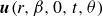 $\boldsymbol{u}(r,\beta ,0,t,\theta )$
as
$\boldsymbol{u}(r,\beta ,0,t,\theta )$
as
 \begin{equation} \boldsymbol{u}(r,\beta ,0,t,\theta ) = \left (\frac {2}{\pi } \left ( \!-\!\cos (\theta )\cos (\beta ) + \frac {r}{\sqrt {a(t)^2-r^2}} \; \sin (\theta ) \right )\right ) \boldsymbol{\underline {\hat {r}}} + \left (1\right )\boldsymbol{\underline {\hat {z}}} \quad \text{for} \quad r \lt a(t). \end{equation}
3. Application of the solution to the droplet impact problem
3.1. Contact line dynamics

Figure 7. Flows over an expanding rising disk have a stagnation point
 $r_1$
at the origin (in the centre of the disk; coordinate directions shown in the bottom right-hand side of each panel) for normal angle impact (a) and off-origin for generalised flow with incidence
$r_1$
at the origin (in the centre of the disk; coordinate directions shown in the bottom right-hand side of each panel) for normal angle impact (a) and off-origin for generalised flow with incidence
 $\theta \neq \pi /2$
(b). In (a), black arrows indicate the flows at
$\theta \neq \pi /2$
(b). In (a), black arrows indicate the flows at
 $z=0$
outside the wet radius in the (expanding) rising disk framework, which deviate from the desired interface positions marked as green arrows on the dashed line (which denotes the droplet boundary) for droplet impact problem.
$z=0$
outside the wet radius in the (expanding) rising disk framework, which deviate from the desired interface positions marked as green arrows on the dashed line (which denotes the droplet boundary) for droplet impact problem.
The flow over a rising disk, in either the SD framework (figure 4
a) or the (expanding) UD framework (figure 4
b), has a stagnation point at the origin (figure 7
a). As might be expected, this stagnation point
 $r_1$
(figure 7
b) is shifted in the generalised flow with incidence (solutions (2.49) and (2.47)) in the range
$r_1$
(figure 7
b) is shifted in the generalised flow with incidence (solutions (2.49) and (2.47)) in the range
 $0 \leqslant \theta \leqslant \pi /2$
. The stagnation point
$0 \leqslant \theta \leqslant \pi /2$
. The stagnation point
 $r_1(\beta ,t,\theta )$
is derived by equating (2.48) to zero,
$r_1(\beta ,t,\theta )$
is derived by equating (2.48) to zero,
 \begin{equation} u_r(r,\beta ,0,t,\theta )= \frac {2}{\pi } \left ( \!-\!\cos (\theta )\cos (\beta ) + \frac {r_1(\beta ,t,\theta )}{\sqrt {a(t)^2-{r_1(\beta ,t,\theta )}^2}} \; \sin (\theta ) \right )=0 \end{equation}
with solution
 \begin{equation} r_1(\beta ,t,\theta )= \sqrt {\frac {a(t)^2}{1+\left ({\tan (\theta )}/{\cos (\beta )}\right )^2}} \quad \text{for }0 \leqslant \theta \leqslant \pi /2. \end{equation}
Equation (3.2) is not valid for
 $\pi /2 \leqslant \beta \lt 3\pi /2$
as there are no stagnation points in the downstream part of the flow. It is noteworthy that
$\pi /2 \leqslant \beta \lt 3\pi /2$
as there are no stagnation points in the downstream part of the flow. It is noteworthy that
 $r_1$
is always less than
$r_1$
is always less than
 $a(t)$
for
$a(t)$
for
 $\theta \gt 0$
(except for the trivial solution at
$\theta \gt 0$
(except for the trivial solution at
 $t=0$
); and as
$t=0$
); and as
 $\theta$
decreases,
$\theta$
decreases,
 $r_1$
shifts from the origin (flow normal to the disk at
$r_1$
shifts from the origin (flow normal to the disk at
 $\theta = \pi /2$
) to the disk edge (uniform flow parallel to the disk surface at
$\theta = \pi /2$
) to the disk edge (uniform flow parallel to the disk surface at
 $\theta =0$
), again as we expect.
$\theta =0$
), again as we expect.

Figure 8. Flows around an expanding rising thin flat disk with incidence
 $\theta =\pi /2$
in the inertial moving frame of reference at velocity
$\theta =\pi /2$
in the inertial moving frame of reference at velocity
 $\boldsymbol{u_0}$
standing at the origin (a), in the static frame of reference standing at the far field at rest (c), and in the moving frame of reference at velocity
$\boldsymbol{u_0}$
standing at the origin (a), in the static frame of reference standing at the far field at rest (c), and in the moving frame of reference at velocity
 $\boldsymbol{a'(t)}$
standing at the right-hand side of the disk edge (e). In the last frame (e), the flow loses axisymmetry and behaves as if with an angle of attack
$\boldsymbol{a'(t)}$
standing at the right-hand side of the disk edge (e). In the last frame (e), the flow loses axisymmetry and behaves as if with an angle of attack
 $\theta _{\!f}$
and stagnates at
$\theta _{\!f}$
and stagnates at
 $r_2$
(relevant streamline not shown). The right-hand column shows similar information for flows with incidence
$r_2$
(relevant streamline not shown). The right-hand column shows similar information for flows with incidence
 $\theta =\pi /3$
(b,d, f). This figure is for
$\theta =\pi /3$
(b,d, f). This figure is for
 $0\leqslant \beta \lt \pi /2$
and
$0\leqslant \beta \lt \pi /2$
and
 $3\pi /2\leqslant \beta \lt 2\pi$
, with the angle
$3\pi /2\leqslant \beta \lt 2\pi$
, with the angle
 $\beta$
defined in figure 9(a).
$\beta$
defined in figure 9(a).
Figure 8 shows the flow field around an expanding rising thin flat disk with incidence
 $\theta =\pi /2$
(figures 8
a, 8
c and 8
e) and
$\theta =\pi /2$
(figures 8
a, 8
c and 8
e) and
 $\theta =\pi /3$
(figures 8
b, 8
d and 8
f) from three different views. For
$\theta =\pi /3$
(figures 8
b, 8
d and 8
f) from three different views. For
 $\theta =\pi /2$
, figure 8(a) (which shows the half-domain only due to axisymmetry) is the flow in the original inertial moving frame of reference at velocity
$\theta =\pi /2$
, figure 8(a) (which shows the half-domain only due to axisymmetry) is the flow in the original inertial moving frame of reference at velocity
 $\boldsymbol{u_0}$
, standing at the origin, and is the same flow as in figure 7(a). The flow stagnates at the disk’s centre and sharply winds around the disk’s edge. This frame of reference describes the physics of a uniform flow falling downwards towards an expanding disk. Figure 8(c) (again, this figure shows the half-domain only, due to axisymmetry) shows the flow in the frame of reference placed in the far field, which is at rest. The flow incident above the surface
$\boldsymbol{u_0}$
, standing at the origin, and is the same flow as in figure 7(a). The flow stagnates at the disk’s centre and sharply winds around the disk’s edge. This frame of reference describes the physics of a uniform flow falling downwards towards an expanding disk. Figure 8(c) (again, this figure shows the half-domain only, due to axisymmetry) shows the flow in the frame of reference placed in the far field, which is at rest. The flow incident above the surface
 $z \geqslant 0$
is diverted in the radial direction by the motion of the disk and sharply winds around at the disk edge. More interestingly, however, figure 8(e) shows another frame of reference, unique to the unsteady disk framework, which moves at the velocity
$z \geqslant 0$
is diverted in the radial direction by the motion of the disk and sharply winds around at the disk edge. More interestingly, however, figure 8(e) shows another frame of reference, unique to the unsteady disk framework, which moves at the velocity
 $\boldsymbol{a'(t)}$
(with the magnitude
$\boldsymbol{a'(t)}$
(with the magnitude
 $a'(t)$
towards the right) standing at (the right-hand side of) the disk edge. In this frame of reference, the flow loses its axisymmetry and the relative velocity approaches the disc at a non-normal angle,
$a'(t)$
towards the right) standing at (the right-hand side of) the disk edge. In this frame of reference, the flow loses its axisymmetry and the relative velocity approaches the disc at a non-normal angle,
 $\theta _{\!f}$
, towards a fixed disk edge. This, again, demonstrates the fact that flow over a flat disk with incidence can be composed by adding a uniform flow at a relative angle of attack. Translating to the moving frame of reference at velocity
$\theta _{\!f}$
, towards a fixed disk edge. This, again, demonstrates the fact that flow over a flat disk with incidence can be composed by adding a uniform flow at a relative angle of attack. Translating to the moving frame of reference at velocity
 $\boldsymbol{a'(t)}$
involves adding a time-dependent uniform flow; and, accordingly, this gives a time-dependent ‘apparent’ angle of attack
$\boldsymbol{a'(t)}$
involves adding a time-dependent uniform flow; and, accordingly, this gives a time-dependent ‘apparent’ angle of attack
 $\theta _{\!f}(\beta ,t)$
. Dividing (2.48) by
$\theta _{\!f}(\beta ,t)$
. Dividing (2.48) by
 $\sin (\theta _{\!f}(\beta ,t))$
and equating to the flow radial velocity in the moving frame, we find
$\sin (\theta _{\!f}(\beta ,t))$
and equating to the flow radial velocity in the moving frame, we find
 \begin{equation} \frac {2}{\pi }\left (\frac {\!-\!\cos (\beta )}{\tan \left (\theta _{\!f}(\beta ,t)\right )} +\frac {r}{\sqrt {a(t)^2-r^2}}\right ) = \frac {2}{\pi }\frac {r}{\sqrt {a(t)^2-r^2}} - a'(t). \end{equation}
Hence,
 \begin{equation} \theta _{\!f}(\beta ,t) = \tan ^{-1} \left ( \frac {2 \cos (\beta )}{\pi \times a'(t)} \right )\!. \end{equation}
Indeed, this apparent angle
 $\theta _{\!f}(\beta ,t)$
is a function of time in the UD framework, and as the velocity of the moving frame
$\theta _{\!f}(\beta ,t)$
is a function of time in the UD framework, and as the velocity of the moving frame
 $a'(t)$
approaches
$a'(t)$
approaches
 $\infty$
, the apparent angle
$\infty$
, the apparent angle
 $\theta _{\!f}(\beta ,t)$
approaches
$\theta _{\!f}(\beta ,t)$
approaches
 $0$
. Nevertheless, it is noted that the angle
$0$
. Nevertheless, it is noted that the angle
 $\theta _{\!f}(\beta ,t)$
is named ‘apparent’ because the flow in this special frame (standing at the disk edge) cannot be obtained simply by substituting the angle
$\theta _{\!f}(\beta ,t)$
is named ‘apparent’ because the flow in this special frame (standing at the disk edge) cannot be obtained simply by substituting the angle
 $\theta _{\!f}(\beta ,t)$
into the solution with incidence in the original frame (standing at the disk centre), but results into a flow with scale
$\theta _{\!f}(\beta ,t)$
into the solution with incidence in the original frame (standing at the disk centre), but results into a flow with scale
 $1/\sin (\theta _{\!f}(\beta ,t))$
. However, this can be resolved by replacing the far-field condition
$1/\sin (\theta _{\!f}(\beta ,t))$
. However, this can be resolved by replacing the far-field condition
 $C= {2}/{\pi }$
with a time-dependent function
$C= {2}/{\pi }$
with a time-dependent function
 $C_{\!f}(\beta ,t)= {2}/({\pi \times \sin (\theta _{\!f}(\beta ,t))})$
as a normalisation.
$C_{\!f}(\beta ,t)= {2}/({\pi \times \sin (\theta _{\!f}(\beta ,t))})$
as a normalisation.
The flow field around the expanding rising thin flat disk in the three different frames of reference is generalised with incidence
 $\theta =\pi /3$
in figures 8(b), 8(d) and 8(f), respectively. Figure 8(b) shows the same flow as in figure 7(b) which has a stagnation point at
$\theta =\pi /3$
in figures 8(b), 8(d) and 8(f), respectively. Figure 8(b) shows the same flow as in figure 7(b) which has a stagnation point at
 $r_1(\beta ,t,\theta )$
(3.2) between the disk surface centre and the wet radius. Figure 8(d) is the flow in the static frame of reference standing in the stationary far field. This frame describes an expanding thin flat disk moving towards the top right-hand direction in an infinite flow domain at rest. Flow above surface
$r_1(\beta ,t,\theta )$
(3.2) between the disk surface centre and the wet radius. Figure 8(d) is the flow in the static frame of reference standing in the stationary far field. This frame describes an expanding thin flat disk moving towards the top right-hand direction in an infinite flow domain at rest. Flow above surface
 $z \geqslant 0$
is, again, diverted towards the radial direction but, at the same time, is also moving towards the left-hand side, owing to the motion of the disk. This composite motion creates a stagnation point away from the disk surface in the direction of the disk motion. It is noted that, due to the extra horizontal motion, the flow winds around at the disk edge with less intensity than the normal impact case and quickly loses the effects of this winding motion away from the disk edge. Figure 8(f) shows the flow with incidence in the frame of reference moving with the edge of the disk at velocity
$z \geqslant 0$
is, again, diverted towards the radial direction but, at the same time, is also moving towards the left-hand side, owing to the motion of the disk. This composite motion creates a stagnation point away from the disk surface in the direction of the disk motion. It is noted that, due to the extra horizontal motion, the flow winds around at the disk edge with less intensity than the normal impact case and quickly loses the effects of this winding motion away from the disk edge. Figure 8(f) shows the flow with incidence in the frame of reference moving with the edge of the disk at velocity
 $\boldsymbol{a'(t)}$
. Comparing with figure 8(e), the ‘apparent’ angle
$\boldsymbol{a'(t)}$
. Comparing with figure 8(e), the ‘apparent’ angle
 $\theta _{\!f}(\beta ,t,\theta )$
in figure 8(f) is greater as a combined result of the flow’s angle of attack
$\theta _{\!f}(\beta ,t,\theta )$
in figure 8(f) is greater as a combined result of the flow’s angle of attack
 $\theta$
in the inertial frame of reference and the effect of the moving frame of reference. Similar to (3.3), dividing (2.48) by
$\theta$
in the inertial frame of reference and the effect of the moving frame of reference. Similar to (3.3), dividing (2.48) by
 $\sin (\theta _{\!f}(\beta ,t,\theta ))$
and multiplying by
$\sin (\theta _{\!f}(\beta ,t,\theta ))$
and multiplying by
 $\sin (\theta )$
, then equating to the flow radial velocity in the moving frame, we derive
$\sin (\theta )$
, then equating to the flow radial velocity in the moving frame, we derive
 \begin{equation} \frac {2}{\pi }\left (\frac {\!-\!\cos (\beta )\sin (\theta )}{\tan (\theta _{\!f}(\beta ,t,\theta ))} +\frac {r \times \sin (\theta )}{\sqrt {a(t)^2-r^2}}\right ) = \frac {2}{\pi }\left (\!-\!\cos (\theta )\cos (\beta ) +\frac {r \times \sin (\theta )}{\sqrt {a(t)^2-r^2}}\right ) - a'(t). \end{equation}
This generalises the solution in (3.4) to
 \begin{equation} \theta _{\!f}(\beta ,t,\theta ) = \tan ^{-1} \left ( \frac {\sin (\theta )}{\cos (\theta ) + {(\pi \times a'(t)}/({2\cos (\beta ))})} \right ) \quad \text{for} \quad 0 \leqslant \theta \leqslant \pi /2. \end{equation}
Equation (3.6) recovers (3.4) at
 $\theta =\pi /2$
. Similarly, this ‘apparent’ angle generates a flow with scale
$\theta =\pi /2$
. Similarly, this ‘apparent’ angle generates a flow with scale
 $\sin (\theta )/\sin (\theta _{\!f}(\beta ,t,\theta ))$
, and can be normalised by the time-dependent far field condition
$\sin (\theta )/\sin (\theta _{\!f}(\beta ,t,\theta ))$
, and can be normalised by the time-dependent far field condition
 $C_{\!f}(\beta ,t)= {(2 \times \sin (\theta )}/({\pi \times\sin (\theta _{\!f}(\beta ,t,\theta )))})$
.
$C_{\!f}(\beta ,t)= {(2 \times \sin (\theta )}/({\pi \times\sin (\theta _{\!f}(\beta ,t,\theta )))})$
.
We emphasise our particular interest in the moving frame of reference at the velocity of the edge of the expanding disk
 $\boldsymbol{a'(t)}$
, as a unique feature of the UD framework which includes the interesting phenomenon of a stagnation point at a radial location
$\boldsymbol{a'(t)}$
, as a unique feature of the UD framework which includes the interesting phenomenon of a stagnation point at a radial location
 $r_2$
on the disk surface which is shown in both figure 8(e) (
$r_2$
on the disk surface which is shown in both figure 8(e) (
 $\theta =\pi /2$
) or figure 8( f) (
$\theta =\pi /2$
) or figure 8( f) (
 $0 \leqslant \theta \lt \pi /2$
). The position of this stagnation point
$0 \leqslant \theta \lt \pi /2$
). The position of this stagnation point
 $r_2(\beta ,t,\theta )$
(below we call
$r_2(\beta ,t,\theta )$
(below we call
 $r_2$
the ‘separation point (for the inner solution)’, to distinguish it from the stagnation point
$r_2$
the ‘separation point (for the inner solution)’, to distinguish it from the stagnation point
 $r_1$
of conventional concept – being stationary in the laboratory frame) can be derived by setting (2.48) for the radial velocity on the surface of the disk, in the moving frame relative to the disk edge, to zero,
$r_1$
of conventional concept – being stationary in the laboratory frame) can be derived by setting (2.48) for the radial velocity on the surface of the disk, in the moving frame relative to the disk edge, to zero,
 \begin{align} u_r(r,\beta ,0,t,\theta )= \frac {2}{\pi } \left ( \!-\!\cos (\theta )\cos (\beta ) + \frac {r_2(\beta ,t,\theta )}{\sqrt {a(t)^2-{r_2(\beta ,t,\theta )}^2}} \; \sin (\theta ) \right ) - a'(t)=0. \end{align}
For
 $\pi /2 \leqslant \beta \lt 3\pi /2$
,
$\pi /2 \leqslant \beta \lt 3\pi /2$
,
 $r_2(\beta ,t,\theta )$
decays in time from a positive value to a value of zero at time
$r_2(\beta ,t,\theta )$
decays in time from a positive value to a value of zero at time
 $t=t_0$
. The value of
$t=t_0$
. The value of
 $t_0$
can be obtained from (3.7) as
$t_0$
can be obtained from (3.7) as
 $\cos (\theta ) \cos (\beta )+ \pi \times a'(t_0)/2=0$
, which solves to
$\cos (\theta ) \cos (\beta )+ \pi \times a'(t_0)/2=0$
, which solves to
 $t_0(\beta ,\theta )=3\pi ^2/(16\cos ^2(\theta )\cos ^2(\beta ))$
. After
$t_0(\beta ,\theta )=3\pi ^2/(16\cos ^2(\theta )\cos ^2(\beta ))$
. After
 $t=t_0$
, we set
$t=t_0$
, we set
 $r_2$
to zero to make the solution valid in polar coordinate. The solution is
$r_2$
to zero to make the solution valid in polar coordinate. The solution is
 \begin{align} &(\text{for }\pi /2\leqslant \beta \lt 3\pi /2) \nonumber \\ &\qquad \quad \quad r_2(\beta ,t,\theta ) = \begin{cases} \sqrt {\frac {a(t)^2}{1+\left ( {\sin (\theta )}/({\cos (\theta ) \cos (\beta )+ (\pi \times a'(t))/{2}}) \right )^2}} & 0\leqslant t \leqslant t_0 \\ 0 & t \gt t_0, \end{cases} \\[-12pt]\nonumber\end{align}
 \begin{align} &(\text{for}\,\, 0\leqslant \beta \lt \pi /2 \text{ and} \,\,3\pi /2\leqslant \beta \lt 2\pi ) \nonumber \\ &\qquad \quad \quad r_2(\beta ,t,\theta ) =\sqrt {\frac {a(t)^2}{1+\left ( {\sin (\theta )}/(\cos (\theta ) \cos (\beta )+ (\pi \times a'(t))/{2}) \right )^2}} \; t \geqslant 0 ,\end{align}
for
 $0 \leqslant \theta \leqslant \pi /2$
; or specifically for
$0 \leqslant \theta \leqslant \pi /2$
; or specifically for
 $\theta = \pi /2$
,
$\theta = \pi /2$
,
 \begin{equation} r_2(\beta ,t,\pi /2)=\sqrt {\frac {a(t)^2}{1+\left ( {2}/({\pi \times a'(t)}) \right )^2}}. \end{equation}
Figure 9(a) presents the difference between the Wagner wet radius
 $a(t)=\sqrt {3t}$
and the separation points of (3.8) (at
$a(t)=\sqrt {3t}$
and the separation points of (3.8) (at
 $\pi /4$
) and (3.9) in polar coordinates (
$\pi /4$
) and (3.9) in polar coordinates (
 $\beta$
,
$\beta$
,
 $r$
) on the impact surface. In particular at
$r$
) on the impact surface. In particular at
 $\beta =0$
or
$\beta =0$
or
 $\pi$
(the view of figure 8), solutions (3.8) and (3.9) are nothing other than substitution of the apparent angles (3.6) and (3.4) into the stagnation (3.2) in the original inertial moving frame of reference,
$\pi$
(the view of figure 8), solutions (3.8) and (3.9) are nothing other than substitution of the apparent angles (3.6) and (3.4) into the stagnation (3.2) in the original inertial moving frame of reference,
 \begin{align} r_2(\beta =0, t,\theta )=r_1(\beta =0,t,\theta _{\!f}) = \sqrt {\frac {a(t)^2}{1+\left ({\sin (\theta )}/({\cos (\theta ) + (\pi \times a'(t))/{2}}) \right )^2}} \quad \text{for} \quad 0 \leqslant \theta \leqslant \pi /2. \end{align}
This is due to the fact that, though the apparent angles (3.4) and (3.6) provide scaled flows of figures 8(e) and 8( f), respectively, these change neither the streamlines, nor hence the stagnation points. Thereby, by the same principle of (3.2) for
 $r_1(\beta ,t,\theta )$
, (3.8) and (3.9) of
$r_1(\beta ,t,\theta )$
, (3.8) and (3.9) of
 $r_2(\beta ,t,\theta )$
are also within the wet radius
$r_2(\beta ,t,\theta )$
are also within the wet radius
 $a(t)$
(except the trivial solution at
$a(t)$
(except the trivial solution at
 $t=0$
). The fact illustrates the dynamics at the wet radius (figure 10) that, in the moving frame of reference at the disk edge, flows are attacking the disk at a separation point (
$t=0$
). The fact illustrates the dynamics at the wet radius (figure 10) that, in the moving frame of reference at the disk edge, flows are attacking the disk at a separation point (
 $r_2$
) which is slightly inboard of the wet radius. In other words, the streamline that connects the wet radius above the disk first ‘overshoots’ to a radius less than the wet radius; but subsequently diverts away (due to the flow separation at
$r_2$
) which is slightly inboard of the wet radius. In other words, the streamline that connects the wet radius above the disk first ‘overshoots’ to a radius less than the wet radius; but subsequently diverts away (due to the flow separation at
 $r_2$
) and winds around the disk edge in an ‘S’ curve.
$r_2$
) and winds around the disk edge in an ‘S’ curve.

Figure 9. Both figures show the top views of droplet impacts with the direction of the flows at an angle
 $\theta$
into the page and from north to south in the plane of the page. (a) The Wagner wet radius
$\theta$
into the page and from north to south in the plane of the page. (a) The Wagner wet radius
 $a(t)=\sqrt {3t}$
and the separation points
$a(t)=\sqrt {3t}$
and the separation points
 $r_2$
(for normal angle impact and for flow with incidence
$r_2$
(for normal angle impact and for flow with incidence
 $\theta =\pi /4$
) are compared in polar coordinates (
$\theta =\pi /4$
) are compared in polar coordinates (
 $\beta$
,
$\beta$
,
 $r$
) set in the impact surface of the disk. To illustrate obvious difference, we compare at the late time of
$r$
) set in the impact surface of the disk. To illustrate obvious difference, we compare at the late time of
 $t=1$
. (b) Comparison between the predicted radius
$t=1$
. (b) Comparison between the predicted radius
 $r_2$
(superimposed as red lines) and the experimental data of water drops’ oblique impacts in García-Geijo et al. (Reference García-Geijo, Riboux and Gordillo2020). The comparisons, showing the analytical solution in the coordinate system with a moving origin at dimensionless velocity
$r_2$
(superimposed as red lines) and the experimental data of water drops’ oblique impacts in García-Geijo et al. (Reference García-Geijo, Riboux and Gordillo2020). The comparisons, showing the analytical solution in the coordinate system with a moving origin at dimensionless velocity
 $\cos(\theta )$
from north to south, are at
$\cos(\theta )$
from north to south, are at
 $\textit{We}\approx 120$
, and impact angles:
$\textit{We}\approx 120$
, and impact angles:
 $\theta =5\pi /12$
(b i);
$\theta =5\pi /12$
(b i);
 $2\pi /3$
(b ii);
$2\pi /3$
(b ii);
 $\pi /4$
(b iii). The horizontal lines indicate the location of the impact point. See García-Geijo et al. (Reference García-Geijo, Riboux and Gordillo2020) for a discussion of the outer line. To be consistent,
$\pi /4$
(b iii). The horizontal lines indicate the location of the impact point. See García-Geijo et al. (Reference García-Geijo, Riboux and Gordillo2020) for a discussion of the outer line. To be consistent,
 $\beta =0$
is defined as the north in both figures.
$\beta =0$
is defined as the north in both figures.

Figure 10. Flow in the moving frame of reference fixed to the disk edge. At the wet radius the flow is attacking the disk at a separation point
 $r_2$
, inboard of the wet radius
$r_2$
, inboard of the wet radius
 $a(t)$
. The streamlines to the right of the separation point first ‘overshoot’ to a radius less than the wet radius, then divert away (due to the flow separation at
$a(t)$
. The streamlines to the right of the separation point first ‘overshoot’ to a radius less than the wet radius, then divert away (due to the flow separation at
 $r_2$
) and wind around the disk edge in an ‘S’-shaped curve. The dashed line outside the disk represents the drop’s free-interface.
$r_2$
) and wind around the disk edge in an ‘S’-shaped curve. The dashed line outside the disk represents the drop’s free-interface.
Figure 9(b) superimposes the predicted separation radius
 $r_2$
onto the experimental data from García-Geijo et al. (Reference García-Geijo, Riboux and Gordillo2020), covering a wide range of impact angles from
$r_2$
onto the experimental data from García-Geijo et al. (Reference García-Geijo, Riboux and Gordillo2020), covering a wide range of impact angles from
 $45^\circ$
to
$45^\circ$
to
 $75^\circ$
, and a super-long timespan up to
$75^\circ$
, and a super-long timespan up to
 $t\gt 8$
. We note that the separation radius
$t\gt 8$
. We note that the separation radius
 $r_2$
is the spatiotemporal boundary separating the droplet and the lamella regions (see § 3.2), and hence is not directly comparable to the maximum spreading radius in the figure, which includes lamella and rim (García-Geijo et al. Reference García-Geijo, Riboux and Gordillo2020). However, it is very difficult, if not impossible, to experimentally locate the locus between the droplet and the lamella, and the present available comparison indeed could provide some useful insights. As we see in figure 9(bi), the oblique analytical solution satisfactorily captures the first-order physics of asymmetric spreading for the large impact angle (close to
$r_2$
is the spatiotemporal boundary separating the droplet and the lamella regions (see § 3.2), and hence is not directly comparable to the maximum spreading radius in the figure, which includes lamella and rim (García-Geijo et al. Reference García-Geijo, Riboux and Gordillo2020). However, it is very difficult, if not impossible, to experimentally locate the locus between the droplet and the lamella, and the present available comparison indeed could provide some useful insights. As we see in figure 9(bi), the oblique analytical solution satisfactorily captures the first-order physics of asymmetric spreading for the large impact angle (close to
 $\pi /2$
) even at late times of
$\pi /2$
) even at late times of
 $t\gt 6$
. At later times or smaller impact angles, we observe that the bottom line of separation radius becomes flat and eventually bends inwards. This is because, in the moving framework of reference, as time increases or impact angle reduces, the advancing speed of the downstream separation line, here denoted as south, becomes large. As a result, the locus of the separation radius
$t\gt 6$
. At later times or smaller impact angles, we observe that the bottom line of separation radius becomes flat and eventually bends inwards. This is because, in the moving framework of reference, as time increases or impact angle reduces, the advancing speed of the downstream separation line, here denoted as south, becomes large. As a result, the locus of the separation radius
 $r_2$
– where advancing speed equals the advancing speed of the wet radius
$r_2$
– where advancing speed equals the advancing speed of the wet radius
 $\sqrt {r/t}/2$
(Riboux & Gordillo Reference Riboux and Gordillo2014), enforced by the Wagner condition – moves upstream. This mechanism is clearer in the frame of reference of figure 9(a). It also agrees with the ‘flat-bottom’ trend of the border of the lamella predicted by García-Geijo et al. (Reference García-Geijo, Riboux and Gordillo2020) at smaller impact angles (note their impact angle is defined as
$\sqrt {r/t}/2$
(Riboux & Gordillo Reference Riboux and Gordillo2014), enforced by the Wagner condition – moves upstream. This mechanism is clearer in the frame of reference of figure 9(a). It also agrees with the ‘flat-bottom’ trend of the border of the lamella predicted by García-Geijo et al. (Reference García-Geijo, Riboux and Gordillo2020) at smaller impact angles (note their impact angle is defined as
 $\chi =\pi /2-\theta$
) and later times (see the bottom row in their figure 4). Particularly, we observe the downstream separation radius bends to the origin in figure 9(b) at
$\chi =\pi /2-\theta$
) and later times (see the bottom row in their figure 4). Particularly, we observe the downstream separation radius bends to the origin in figure 9(b) at
 $\theta =\pi /4$
for
$\theta =\pi /4$
for
 $t\gt 4$
. We provide two reasons for this overestimated behaviour: (i) the classical wet radius
$t\gt 4$
. We provide two reasons for this overestimated behaviour: (i) the classical wet radius
 $\sqrt {3t}$
was derived under the assumption of normal impact (Wagner Reference Wagner1932; Riboux & Gordillo Reference Riboux and Gordillo2014) while a proper wet radius model considering the asymmetric spreading shape would increase the velocity threshold of the separation point; and (ii) viscosity effects are omitted in the present potential theory, which could effectively mitigate the advancing speed of the separation line, even in regimes that are often considered inviscid (Sanjay & Lohse Reference Sanjay and Lohse2025). Nevertheless, we note that even the first frames (
$\sqrt {3t}$
was derived under the assumption of normal impact (Wagner Reference Wagner1932; Riboux & Gordillo Reference Riboux and Gordillo2014) while a proper wet radius model considering the asymmetric spreading shape would increase the velocity threshold of the separation point; and (ii) viscosity effects are omitted in the present potential theory, which could effectively mitigate the advancing speed of the separation line, even in regimes that are often considered inviscid (Sanjay & Lohse Reference Sanjay and Lohse2025). Nevertheless, we note that even the first frames (
 $t\gt 1$
) of the compared cases in figure 9(b) fall into the late-time regime while the present analytical model is derived (mainly) for early and intermediate times (
$t\gt 1$
) of the compared cases in figure 9(b) fall into the late-time regime while the present analytical model is derived (mainly) for early and intermediate times (
 $t\lt 0.27$
, see § 5), where viscosity and capillary effects can be omitted (Eggers et al. Reference Eggers, Fontelos, Josserand and Zaleski2010).
$t\lt 0.27$
, see § 5), where viscosity and capillary effects can be omitted (Eggers et al. Reference Eggers, Fontelos, Josserand and Zaleski2010).
3.2. Wagner condition and a solution to the droplet impact problem
From now on, we specifically consider the application of the above UD framework to the droplet impact problem (figure 3 a).
The literature associated with droplet impact problem has conventionally used, for the water-entry problem, both the intersection radius
 $\sqrt {2t}$
(Howison et al. Reference Howison, Ockendon and Wilson1991) and the wet radius
$\sqrt {2t}$
(Howison et al. Reference Howison, Ockendon and Wilson1991) and the wet radius
 $\sqrt {3t}$
(Wagner Reference Wagner1932; Philippi et al. Reference Philippi, Lagrée and Antkowiak2016) for
$\sqrt {3t}$
(Wagner Reference Wagner1932; Philippi et al. Reference Philippi, Lagrée and Antkowiak2016) for
 $a(t)$
. Notably, the wet radius
$a(t)$
. Notably, the wet radius
 $\sqrt {3t}$
is derived from the Wagner condition for normal impact (i.e.
$\sqrt {3t}$
is derived from the Wagner condition for normal impact (i.e.
 $\theta =\pi /2$
). In the analysis below, we will assume
$\theta =\pi /2$
). In the analysis below, we will assume
 $a(t)=\sqrt {\lambda t}$
for general
$a(t)=\sqrt {\lambda t}$
for general
 $\lambda \gt 2$
.
$\lambda \gt 2$
.
In § 3.1, we established the existence of a separation point
 $r_2$
in the UD framework, in the moving frame of reference at the disk edge; and we have derived its radial position in (3.8) and (3.9). The ratio between
$r_2$
in the UD framework, in the moving frame of reference at the disk edge; and we have derived its radial position in (3.8) and (3.9). The ratio between
 $r_2$
and
$r_2$
and
 $a$
is not constant due to the non-inertial moving frame of reference at the disk edge. We note that this dynamic ratio is a unique feature of the UD framework, and cannot be obtained from the SSD framework (Philippi et al. Reference Philippi, Lagrée and Antkowiak2016) where the ratio would be fixed in self-similar space and is equivalent to the ratio at
$a$
is not constant due to the non-inertial moving frame of reference at the disk edge. We note that this dynamic ratio is a unique feature of the UD framework, and cannot be obtained from the SSD framework (Philippi et al. Reference Philippi, Lagrée and Antkowiak2016) where the ratio would be fixed in self-similar space and is equivalent to the ratio at
 $t=1$
of the present UD framework. In the current UD framework, the ratio between
$t=1$
of the present UD framework. In the current UD framework, the ratio between
 $r_2$
and
$r_2$
and
 $a$
varies from
$a$
varies from
 $1$
and
$1$
and
 $0$
. This corresponds to
$0$
. This corresponds to
 $r_2$
monotonically shifting from
$r_2$
monotonically shifting from
 $a$
to the asymptotic limit
$a$
to the asymptotic limit
 $r_1$
in time, which is the stagnation point in the original moving frame of reference, as in the original moving frame due to the relatively negligible velocity of disk expansion at late time.
$r_1$
in time, which is the stagnation point in the original moving frame of reference, as in the original moving frame due to the relatively negligible velocity of disk expansion at late time.
Wagner’s condition (Wagner Reference Wagner1932) is useful for linking the kinematics of the horizontal expansion of the wet radius to the vertical motion of the free surface in the context of droplet impact problem. In other words, when the downward motion of the droplet causes the free surface of the droplet to meet the solid surface, it becomes the turnover point: namely, the wet radius. See, in particular, figure
 $5$
of Philippi et al. (Reference Philippi, Lagrée and Antkowiak2016) as well as Riboux & Gordillo (Reference Riboux and Gordillo2014) and Negus et al. (Reference Negus, Moore, Oliver and Cimpeanu2021). This argument suggests a deduction that not only is the position of the turnover point determined by the time when a point on the curved droplet–air interface reaches the disk surface due to the interface’s predominantly vertical motion, but also that the horizontal expanding velocity at the turnover point should be determined by the radial velocity of this particular point when it reaches the disk. Therefore, the separation point
$5$
of Philippi et al. (Reference Philippi, Lagrée and Antkowiak2016) as well as Riboux & Gordillo (Reference Riboux and Gordillo2014) and Negus et al. (Reference Negus, Moore, Oliver and Cimpeanu2021). This argument suggests a deduction that not only is the position of the turnover point determined by the time when a point on the curved droplet–air interface reaches the disk surface due to the interface’s predominantly vertical motion, but also that the horizontal expanding velocity at the turnover point should be determined by the radial velocity of this particular point when it reaches the disk. Therefore, the separation point
 $r_2$
, at which the flow has the same radial velocity as the disk’s velocity of expansion, is the particular turnover point in our expanding water-entry analogy (yellow crosses in figure 5
c). This provides us with the first reason to choose
$r_2$
, at which the flow has the same radial velocity as the disk’s velocity of expansion, is the particular turnover point in our expanding water-entry analogy (yellow crosses in figure 5
c). This provides us with the first reason to choose
 $r_2$
as the point at which we stop the solution. This leads to the solution of the expanding water-entry analogy, in the inertial moving frame of reference at the disk centre, as
$r_2$
as the point at which we stop the solution. This leads to the solution of the expanding water-entry analogy, in the inertial moving frame of reference at the disk centre, as
 \begin{align} \boldsymbol{u}(r,\beta ,0,t,\theta ) = \left (\frac {2}{\pi } \left ( \!-\!\cos (\theta )\cos (\beta ) + \frac {r}{\sqrt {a(t)^2-r^2}} \; \sin (\theta ) \right )\right ) \boldsymbol{\underline {\hat {r}}} + \left (0\right )\boldsymbol{\underline {\hat {z}}} \quad \text{for} \quad r \leqslant r_2(\beta ,t,\theta ) \end{align}
 \begin{align} \frac {\partial \phi }{\partial t}(r,\beta ,0,t,\theta ) =- \frac {2}{\pi } \frac {a(t)a'(t)\sin (\theta )}{\sqrt {a(t)^2-r^2}} \quad \text{for} \quad r \leqslant r_2(\beta ,t,\theta ) \end{align}
evaluated up to
 $r_2$
((3.8) for
$r_2$
((3.8) for
 $0 \leqslant \theta \leqslant \pi /2$
or (3.9) for
$0 \leqslant \theta \leqslant \pi /2$
or (3.9) for
 $\theta = \pi /2$
). We propose that the set of (3.11) and (3.12) for the expanding water-entry analogy is a solution to the droplet impact problem at the solid surface.
$\theta = \pi /2$
). We propose that the set of (3.11) and (3.12) for the expanding water-entry analogy is a solution to the droplet impact problem at the solid surface.
3.3. Impact pressure on the solid surface
From (2.9), (3.11) and (3.12), we recover the unsteady form of the Bernoulli pressure on the solid surface upon droplet impact,
 \begin{align} p(r,\beta ,0,t,\theta ) &= b(t,\theta ) - \frac {{u_r}^2}{2} -\frac {\partial \phi }{\partial t} \nonumber \\ &= b(t,\theta ) - \frac {2}{\pi ^2} \left ( \cos (\theta ) \cos (\beta )- \frac {r}{\sqrt {a(t)^2-r^2}} \; \sin (\theta ) \right )^2 \nonumber \\ &\;\;\;\;\;\;\;\;\;\;\;\;\;\;\;\;\;\;\;\;\;\;\;\;\;\;\;\;\;\;\;\;+ \frac {2}{\pi } \frac {a(t)a'(t)\sin (\theta )}{\sqrt {a(t)^2-r^2}} \quad \text{for} \quad r \leqslant r_2(\beta ,t,\theta ) \end{align}
where the Bernoulli constant
 $b(t,\theta )$
is generalised with incidence. Also, since we neglect viscosity and surface tension in the current ideal flow field framework, by continuity of normal stress at the liquid boundary, we have
$b(t,\theta )$
is generalised with incidence. Also, since we neglect viscosity and surface tension in the current ideal flow field framework, by continuity of normal stress at the liquid boundary, we have
 $p=0$
at all free interfaces. Applying (2.9) at the droplet top interface, where the flow is moving downwards with unit (dimensionless) velocity because the bulk of the droplet is unaffected by the impact – at least at the earlier stages of impact (Riboux & Gordillo Reference Riboux and Gordillo2014), we obtain
$p=0$
at all free interfaces. Applying (2.9) at the droplet top interface, where the flow is moving downwards with unit (dimensionless) velocity because the bulk of the droplet is unaffected by the impact – at least at the earlier stages of impact (Riboux & Gordillo Reference Riboux and Gordillo2014), we obtain
 $b(t,\theta ) = 1/2$
for
$b(t,\theta ) = 1/2$
for
 $t \geqslant 0$
and
$t \geqslant 0$
and
 $0 \leqslant \theta \leqslant \pi /2$
.
$0 \leqslant \theta \leqslant \pi /2$
.
The impact pressure (3.13) has a negative singularity at the wet radius
 $a(t)$
for
$a(t)$
for
 $\theta \gt 0$
. Nevertheless, the singularity is not of any concern for the solution proposed in the current paper, due to the fact that
$\theta \gt 0$
. Nevertheless, the singularity is not of any concern for the solution proposed in the current paper, due to the fact that
 $r_2(\beta ,t,\theta )$
is always less than
$r_2(\beta ,t,\theta )$
is always less than
 $a(t)$
. This provides us with a second reason to choose
$a(t)$
. This provides us with a second reason to choose
 $r_2$
as the point at which we stop the solution: the ‘expanding rising disk’ analogue fails to describe the droplet impact problem near the wet radius. The reason can be inferred from the well-known negative pressure singularity at the disk edge of the two-dimensional potential flow over a disk/fence (figure 5
a), where the flow needs to wind over the object immediately, and hence at infinite velocity. For the current three-dimensional flow, this is illustrated in figures 8(c) and 8(d). Flow streamlines are winding around the disk edge, creating a pressure minimum at the disk edge. This is not to be expected at the wet radius in a droplet impact problem, in which the correct free interface Bernoulli condition
$r_2$
as the point at which we stop the solution: the ‘expanding rising disk’ analogue fails to describe the droplet impact problem near the wet radius. The reason can be inferred from the well-known negative pressure singularity at the disk edge of the two-dimensional potential flow over a disk/fence (figure 5
a), where the flow needs to wind over the object immediately, and hence at infinite velocity. For the current three-dimensional flow, this is illustrated in figures 8(c) and 8(d). Flow streamlines are winding around the disk edge, creating a pressure minimum at the disk edge. This is not to be expected at the wet radius in a droplet impact problem, in which the correct free interface Bernoulli condition
 $\partial \phi / \partial t + {(\boldsymbol{\nabla }\phi )}^2/2=0$
has been replaced by
$\partial \phi / \partial t + {(\boldsymbol{\nabla }\phi )}^2/2=0$
has been replaced by
 $\phi =0$
at the wet radius
$\phi =0$
at the wet radius
 $a$
in the current UD framework (figure 4
b) (Korobkin & Scolan Reference Korobkin and Scolan2006). In other words, the approach of simple inviscid potential flow theory cannot lead to correct solutions to the complex phenomenon (droplet impact problem) at the wet radius (Cointe & Armand Reference Cointe and Armand1987) where, in practice, liquid viscosity and surface tension should play important roles (Gordillo et al. Reference Gordillo, Riboux and Quintero2019). In previous work, where solutions are conventionally evaluated up to the wet radius, the phenomenon of a singularity has also been noticed in several works on the water-entry problem (Wagner Reference Wagner1932; Logvinovich Reference Logvinovich1969; Faltinsen & Wu Reference Faltinsen and Wu2001). Interestingly, the unsteady term of (3.13) also has a (positive) singularity at the wet radius due to the unsteady expanding motion of the disk, which has been noted by Cointe & Armand (Reference Cointe and Armand1987), Tassin et al. (Reference Tassin, Jacques, El Malki Alaoui, Nême and Leblé2010) and Philippi et al. (Reference Philippi, Lagrée and Antkowiak2016). But the nature of the positive singularity has a smaller order of magnitude than the negative pressure singularity, and therefore the combined solution exhibits the negative singularity only as a result of the infinite flow velocity. A conventional approach to resolve the singularity was first proposed by Wagner (Reference Wagner1932) for the water-entry problem, analytically derived by Cointe & Armand (Reference Cointe and Armand1987) in two-dimensions, and Scolan (Reference Scolan2004) in three-dimensions, and adapted for the droplet impact problem by Negus et al. (Reference Negus, Moore, Oliver and Cimpeanu2021). The approach is to asymptotically compose the original singular solution with an extra splashing solution in the so-called inner region at the wet radius where the original singular solution breaks down.
$a$
in the current UD framework (figure 4
b) (Korobkin & Scolan Reference Korobkin and Scolan2006). In other words, the approach of simple inviscid potential flow theory cannot lead to correct solutions to the complex phenomenon (droplet impact problem) at the wet radius (Cointe & Armand Reference Cointe and Armand1987) where, in practice, liquid viscosity and surface tension should play important roles (Gordillo et al. Reference Gordillo, Riboux and Quintero2019). In previous work, where solutions are conventionally evaluated up to the wet radius, the phenomenon of a singularity has also been noticed in several works on the water-entry problem (Wagner Reference Wagner1932; Logvinovich Reference Logvinovich1969; Faltinsen & Wu Reference Faltinsen and Wu2001). Interestingly, the unsteady term of (3.13) also has a (positive) singularity at the wet radius due to the unsteady expanding motion of the disk, which has been noted by Cointe & Armand (Reference Cointe and Armand1987), Tassin et al. (Reference Tassin, Jacques, El Malki Alaoui, Nême and Leblé2010) and Philippi et al. (Reference Philippi, Lagrée and Antkowiak2016). But the nature of the positive singularity has a smaller order of magnitude than the negative pressure singularity, and therefore the combined solution exhibits the negative singularity only as a result of the infinite flow velocity. A conventional approach to resolve the singularity was first proposed by Wagner (Reference Wagner1932) for the water-entry problem, analytically derived by Cointe & Armand (Reference Cointe and Armand1987) in two-dimensions, and Scolan (Reference Scolan2004) in three-dimensions, and adapted for the droplet impact problem by Negus et al. (Reference Negus, Moore, Oliver and Cimpeanu2021). The approach is to asymptotically compose the original singular solution with an extra splashing solution in the so-called inner region at the wet radius where the original singular solution breaks down.
A direct, and important, result from the existence of the two opposite-sign terms in (3.13) is the so-called ring-pattern pressure peak near, but inboard of, the wet radius. The pressure peak is produced by the balance between the steady and unsteady Bernoulli terms, and may explain the ring-shaped cracks in the surface observed in various experiments (Field Reference Field1966; Field et al. Reference Field, Lesser and Dear1985). Analytically, we can derive the position
 $r_{\textit{max}}(t,\theta )$
and the peak pressure value
$r_{\textit{max}}(t,\theta )$
and the peak pressure value
 $p_{\textit{max}}(\beta ,t,\theta )$
by differentiating (3.13),
$p_{\textit{max}}(\beta ,t,\theta )$
by differentiating (3.13),
 \begin{equation} \frac {\partial p}{\partial r} (r_{\textit{max}},\beta ,0,t,\theta )= \frac {4}{\pi ^2} \left ( \frac {a^2\sin (\theta )\cos (\theta )\cos (\beta )}{(a^2-{r_{\textit{max}}}^2)^{3/2}} - \frac {{r_{\textit{max}}}a^2}{{(a^2-{r_{\textit{max}}}^2)}^2} \right ) + \frac {2}{\pi } \frac {aa'\sin (\theta ){r_{\textit{max}}}}{(a^2-{r_{\textit{max}}}^2)^{3/2}} = 0 \end{equation}
to solve for
 $0 \lt r_{\textit{max}}(\beta ,t,\theta ) \leqslant r_2(\beta ,t,\theta )$
, and hence
$0 \lt r_{\textit{max}}(\beta ,t,\theta ) \leqslant r_2(\beta ,t,\theta )$
, and hence
 \begin{equation} p_{\textit{max}}(\beta ,t,\theta )=p(r_{\textit{max}},\beta ,0,t,\theta ). \end{equation}
Regarding solutions outside the wet radius, we have derived the velocity field of (2.33) and the unsteady Bernoulli term
 $\partial \phi / \partial t$
of (2.42) for the expanding rising disk with flow at incidence
$\partial \phi / \partial t$
of (2.42) for the expanding rising disk with flow at incidence
 $\pi /2$
. Also, in § 3.1, we have seen the ‘S’ shape of the streamlines outside the separation point, which, in our expanding water-entry analogy, are interpreted as the flow at the free interfaces of an impacting droplet (see figure 8
e). The nature of the separation point,
$\pi /2$
. Also, in § 3.1, we have seen the ‘S’ shape of the streamlines outside the separation point, which, in our expanding water-entry analogy, are interpreted as the flow at the free interfaces of an impacting droplet (see figure 8
e). The nature of the separation point,
 $r_2$
, indicates the fact that the ‘S’ shapes on the interfaces have greater radial velocity than the expanding wet radius. However, this apparently contradicts what we find on the velocity vectors (2.33) which, outside the wet radius, have no radial component and are purely downward-directed in the original moving frame of reference at the disk centre. The apparent contradiction stems from the fact that solutions (2.33) and (2.42) describe the flows at
$r_2$
, indicates the fact that the ‘S’ shapes on the interfaces have greater radial velocity than the expanding wet radius. However, this apparently contradicts what we find on the velocity vectors (2.33) which, outside the wet radius, have no radial component and are purely downward-directed in the original moving frame of reference at the disk centre. The apparent contradiction stems from the fact that solutions (2.33) and (2.42) describe the flows at
 $z=0$
in the UD framework, which is totally different from the position of the droplet interface in droplet impact problem (figure 3). The difference is illustrated in figure 7(a), where the black arrows are the solutions outside the wet radius while the green arrows (on the imaginary droplet interface) indicate the desired interface solution for droplet impact problem. Similar to the classic water-entry problem (Zhao & Faltinsen Reference Zhao and Faltinsen1993; Korobkin Reference Korobkin2004), the accuracy in approximating the desired solution on the droplet interface by the solution to the UD problem depends on the deadrise angle of the obstacle which, in the case of spherical droplet, increases from zero to normal angle as the distance from the wet radius increases. Therefore, solutions outside the wet radius are not of the concern in the current study; and it is interesting to note that the conventional method of composing a local splash solution at the wet radius is not applicable also for non-small deadrise angles, due to the order mismatch between the Bernoulli term and the splash solution in the inner region (Zhao & Faltinsen Reference Zhao and Faltinsen1993).
$z=0$
in the UD framework, which is totally different from the position of the droplet interface in droplet impact problem (figure 3). The difference is illustrated in figure 7(a), where the black arrows are the solutions outside the wet radius while the green arrows (on the imaginary droplet interface) indicate the desired interface solution for droplet impact problem. Similar to the classic water-entry problem (Zhao & Faltinsen Reference Zhao and Faltinsen1993; Korobkin Reference Korobkin2004), the accuracy in approximating the desired solution on the droplet interface by the solution to the UD problem depends on the deadrise angle of the obstacle which, in the case of spherical droplet, increases from zero to normal angle as the distance from the wet radius increases. Therefore, solutions outside the wet radius are not of the concern in the current study; and it is interesting to note that the conventional method of composing a local splash solution at the wet radius is not applicable also for non-small deadrise angles, due to the order mismatch between the Bernoulli term and the splash solution in the inner region (Zhao & Faltinsen Reference Zhao and Faltinsen1993).

Figure 11. Comparisons between the present analytical pressure model with various results in the literature between
 $t=2\times 10^{-2}$
and
$t=2\times 10^{-2}$
and
 $t=10^{-1}$
at half-domain (without loss of generality at
$t=10^{-1}$
at half-domain (without loss of generality at
 $\beta =0$
) (a–c), and full domain (without loss of generality at
$\beta =0$
) (a–c), and full domain (without loss of generality at
 $\beta =0$
and
$\beta =0$
and
 $\pi$
) (e). In the latter, the generalised present model with incidence
$\pi$
) (e). In the latter, the generalised present model with incidence
 $\pi /4$
is also superimposed. Bernoulli constants are removed from all pressure profiles for consistency. The pressure profile at
$\pi /4$
is also superimposed. Bernoulli constants are removed from all pressure profiles for consistency. The pressure profile at
 $t=10^{-1}$
is zoomed-in at the wet radius (d) to illustrate the relative positions between
$t=10^{-1}$
is zoomed-in at the wet radius (d) to illustrate the relative positions between
 $r_{\textit{max}}$
,
$r_{\textit{max}}$
,
 $r_2$
,
$r_2$
,
 $r_*$
, and the wet radius
$r_*$
, and the wet radius
 $a$
at normal angle of incidence. Note, in particular, that the separation point
$a$
at normal angle of incidence. Note, in particular, that the separation point
 $r_2$
is found to be very close to the radius of pressure maximum,
$r_2$
is found to be very close to the radius of pressure maximum,
 $r_{\textit{max}}$
.
$r_{\textit{max}}$
.
We now compare the pressure solution in (3.13) with some typical analytical pressure solutions in the literature (presented in the axisymmetric forms) in figure 11. It is noted that, for all pressure solutions in the comparison,
 $a(t)$
has the value of
$a(t)$
has the value of
 $\sqrt {3 t}$
and the Bernoulli constant
$\sqrt {3 t}$
and the Bernoulli constant
 $b(t,\theta )$
is removed for consistency, since the values of
$b(t,\theta )$
is removed for consistency, since the values of
 $a(t)$
and
$a(t)$
and
 $b(t,\theta )$
vary in different methods and applications. Figure 11(a) compares the analytical pressure in the literature on droplet impact at normal angle at time
$b(t,\theta )$
vary in different methods and applications. Figure 11(a) compares the analytical pressure in the literature on droplet impact at normal angle at time
 $t=0.02{-}0.1$
with time step
$t=0.02{-}0.1$
with time step
 $\Delta t=0.02$
. The proposed solution in the current work compares well, in terms of the shapes and the magnitude of the peak pressure, especially at small
$\Delta t=0.02$
. The proposed solution in the current work compares well, in terms of the shapes and the magnitude of the peak pressure, especially at small
 $t$
, with the other two in the literature. Specifically, Philippi et al. (Reference Philippi, Lagrée and Antkowiak2016) considers only the unsteady term of the Bernoulli (2.9), and hence the pressure is monotonic at each time and rises to the positive singularity at the wet radius. Negus et al. (Reference Negus, Moore, Oliver and Cimpeanu2021) composes the splash solution at the wet radius, and correspondingly their solution shows the existence of a ‘tail’ beyond the wet radius, which expands in extent with time. The composed splash solution leads pressure to zero. Figures 11(b) and 11(c) compare also the analytical pressure given in the literature on the water-entry problem at normal angle over the same time period. The solution by Logvinovich (Reference Logvinovich1969) turns out to be ‘exactly the same’ as the derived solution in this paper, but is continued to greater radius. This is because the derived pressure (3.13) at
$t$
, with the other two in the literature. Specifically, Philippi et al. (Reference Philippi, Lagrée and Antkowiak2016) considers only the unsteady term of the Bernoulli (2.9), and hence the pressure is monotonic at each time and rises to the positive singularity at the wet radius. Negus et al. (Reference Negus, Moore, Oliver and Cimpeanu2021) composes the splash solution at the wet radius, and correspondingly their solution shows the existence of a ‘tail’ beyond the wet radius, which expands in extent with time. The composed splash solution leads pressure to zero. Figures 11(b) and 11(c) compare also the analytical pressure given in the literature on the water-entry problem at normal angle over the same time period. The solution by Logvinovich (Reference Logvinovich1969) turns out to be ‘exactly the same’ as the derived solution in this paper, but is continued to greater radius. This is because the derived pressure (3.13) at
 $\theta =\pi /2$
recovers the exact pressure expression in Logvinovich (Reference Logvinovich1969); however, Logvinovich evaluates the expression to the radius
$\theta =\pi /2$
recovers the exact pressure expression in Logvinovich (Reference Logvinovich1969); however, Logvinovich evaluates the expression to the radius
 $r_*$
(see (3.16) below) where the pressure is zero while (3.13) is evaluated no farther than the separation point
$r_*$
(see (3.16) below) where the pressure is zero while (3.13) is evaluated no farther than the separation point
 $r_2$
. The composed solution in Zhao & Faltinsen (Reference Zhao and Faltinsen1993), Scolan (Reference Scolan2004), Wilson (Reference Wilson1989) and Howison et al. (Reference Howison, Ockendon and Wilson1991) is of the same form for flat deadrise angle, and is the precursor of the Negus et al. (Reference Negus, Moore, Oliver and Cimpeanu2021) solution. The difference between the two sets of solutions is the shift of
$r_2$
. The composed solution in Zhao & Faltinsen (Reference Zhao and Faltinsen1993), Scolan (Reference Scolan2004), Wilson (Reference Wilson1989) and Howison et al. (Reference Howison, Ockendon and Wilson1991) is of the same form for flat deadrise angle, and is the precursor of the Negus et al. (Reference Negus, Moore, Oliver and Cimpeanu2021) solution. The difference between the two sets of solutions is the shift of
 $+6\delta /\pi$
in the radial direction, due to the difference in the location of the stagnation points in droplet impact and water-entry problems (Oliver Reference Oliver2002). Similarly, Cointe & Armand (Reference Cointe and Armand1987) and Faltinsen & Wu (Reference Faltinsen and Wu2001), instead of asymptotic analysis, use the Heaviside function to ‘peg’ the Bernoulli pressure to the splash solution, respectively, either at the radius where the unsteady Bernoulli term equals the splash pressure peak, or at the radius where the entire Bernoulli pressure equals the splash pressure peak (here as
$+6\delta /\pi$
in the radial direction, due to the difference in the location of the stagnation points in droplet impact and water-entry problems (Oliver Reference Oliver2002). Similarly, Cointe & Armand (Reference Cointe and Armand1987) and Faltinsen & Wu (Reference Faltinsen and Wu2001), instead of asymptotic analysis, use the Heaviside function to ‘peg’ the Bernoulli pressure to the splash solution, respectively, either at the radius where the unsteady Bernoulli term equals the splash pressure peak, or at the radius where the entire Bernoulli pressure equals the splash pressure peak (here as
 $r_{s2}$
in figure 11
c). Both pressure distributions by Cointe & Armand (Reference Cointe and Armand1987) and Faltinsen & Wu (Reference Faltinsen and Wu2001) compare well with the value of pressure peaks from (3.13), but differ in terms of the radial extent. Finally, figure 11(e) mixes the typical solutions from droplet impact and water-entry literature, and compares them with (3.13) at flow incidence
$r_{s2}$
in figure 11
c). Both pressure distributions by Cointe & Armand (Reference Cointe and Armand1987) and Faltinsen & Wu (Reference Faltinsen and Wu2001) compare well with the value of pressure peaks from (3.13), but differ in terms of the radial extent. Finally, figure 11(e) mixes the typical solutions from droplet impact and water-entry literature, and compares them with (3.13) at flow incidence
 $\theta = \pi /4$
. Due to loss of axisymmetry of (3.13) at non-normal angle of incidence, the pressure distributions are shown in the meridional plane; note, however, that all pressures from the literature are symmetrical in figure 11(e). For pressure (3.13) at
$\theta = \pi /4$
. Due to loss of axisymmetry of (3.13) at non-normal angle of incidence, the pressure distributions are shown in the meridional plane; note, however, that all pressures from the literature are symmetrical in figure 11(e). For pressure (3.13) at
 $\theta = \pi /4$
(related to flow from right (positive
$\theta = \pi /4$
(related to flow from right (positive
 $r$
-axis with
$r$
-axis with
 $\beta =0$
) to left (negative
$\beta =0$
) to left (negative
 $r$
-axis with
$r$
-axis with
 $\beta =\pi$
)), pressure distribution is ‘tilted’ towards the right-hand side and has a higher pressure peak near the right-hand separation
$\beta =\pi$
)), pressure distribution is ‘tilted’ towards the right-hand side and has a higher pressure peak near the right-hand separation
 $r=+r_2$
; meanwhile, interestingly, the pressure at the centre,
$r=+r_2$
; meanwhile, interestingly, the pressure at the centre,
 $r=0$
, is always lower than the centre pressure would have been at normal angle of impact (refer to the centre pressure value of Logvinovich in the same figure).
$r=0$
, is always lower than the centre pressure would have been at normal angle of impact (refer to the centre pressure value of Logvinovich in the same figure).
Equation (3.13) (without Bernoulli constant
 $b(t,\theta )$
) reaches zero pressure at radius
$b(t,\theta )$
) reaches zero pressure at radius
 $r_*(t,\theta )$
where the magnitudes of the positive unsteady Bernoulli term and the negative nonlinear Bernoulli term are equal. This leads to the equation for
$r_*(t,\theta )$
where the magnitudes of the positive unsteady Bernoulli term and the negative nonlinear Bernoulli term are equal. This leads to the equation for
 $r_*(\beta ,t,\theta ) \leqslant a(t)$
as
$r_*(\beta ,t,\theta ) \leqslant a(t)$
as
 \begin{align} r_*^2\sin ^2(\theta )-\left (2 r_*\cos (\theta )\sin (\theta )+\pi a(t) a'(t) \sin (\theta )\right )\sqrt {a(t)^2-{r_*}^2}+{\cos }^2(\theta )\big (a(t)^2-{r_*}^2\big )=0. \end{align}
Equation (3.16) is a general quartic equation with a lengthy root formula; however, specifically at
 $\theta =\pi /2$
, it simplifies to a quadratic equation on
$\theta =\pi /2$
, it simplifies to a quadratic equation on
 ${r_*}^2$
,
${r_*}^2$
,
 \begin{equation} \frac {1}{(\pi a(t) a'(t))^2}\big ({r_*}^2\big )^2 +\big ({r_*}^2\big )^2-a(t)^2=0 \end{equation}
which can be easily solved and obtains the only reasonable positive real root,
 \begin{equation} r_*(\beta ,t,\pi /2)=\sqrt {\frac {Q}{2} \left ( \sqrt {1+\frac {4a(t)^2}{Q}}-1 \right )} \end{equation}
where
 $Q=(\pi a(t) a'(t))^2$
is a constant for
$Q=(\pi a(t) a'(t))^2$
is a constant for
 $a(t)= O(\sqrt {t})$
. We note that Logvinovich (Reference Logvinovich1969) considered the two-dimensional problem and derived (1.8) for
$a(t)= O(\sqrt {t})$
. We note that Logvinovich (Reference Logvinovich1969) considered the two-dimensional problem and derived (1.8) for
 $x_*(t)$
, while (3.18) at
$x_*(t)$
, while (3.18) at
 $\theta =\pi /2$
is the corresponding point in the axisymmetric potential flow. Similarly, at
$\theta =\pi /2$
is the corresponding point in the axisymmetric potential flow. Similarly, at
 $\theta =\pi /2$
, the quartic (3.14) is greatly simplified, and the solution can be obtained as
$\theta =\pi /2$
, the quartic (3.14) is greatly simplified, and the solution can be obtained as
 \begin{equation} r_{\textit{max}}(\beta ,t,\pi /2)=\sqrt {a(t)^2-\frac {4a(t)^4}{Q}} \end{equation}
and hence the dimensionless peak pressure (without Bernoulli constant
 $b(t,\theta )$
) is
$b(t,\theta )$
) is
 \begin{equation} p_{\textit{max}}(\beta ,t,\pi /2)=\frac {Q}{2\pi ^2a(t)^2} \left (1+ \frac {4a(t)^2}{Q}\right )\!. \end{equation}
It is not obvious whether
 $r_*(\beta ,t,\pi /2)$
and
$r_*(\beta ,t,\pi /2)$
and
 $r_{\textit{max}}(\beta ,t,\pi /2)$
are always inboard of the separation point
$r_{\textit{max}}(\beta ,t,\pi /2)$
are always inboard of the separation point
 $r_2(\beta ,t,\pi /2)$
of (3.9) for general
$r_2(\beta ,t,\pi /2)$
of (3.9) for general
 $a(t)$
; but specifically for
$a(t)$
; but specifically for
 $a(t)=\sqrt {3t}$
,
$a(t)=\sqrt {3t}$
,
 $r_*(\beta ,t,\pi /2)$
is greater than
$r_*(\beta ,t,\pi /2)$
is greater than
 $r_2(\beta ,t,\pi /2)$
at all time
$r_2(\beta ,t,\pi /2)$
at all time
 $t\gt 0$
. Therefore, the proposed pressure of (3.13) for the droplet impact problem is always non-negative. The relative positions between
$t\gt 0$
. Therefore, the proposed pressure of (3.13) for the droplet impact problem is always non-negative. The relative positions between
 $r_{\textit{max}}(\beta ,t,\pi /2)$
,
$r_{\textit{max}}(\beta ,t,\pi /2)$
,
 $r_2(\beta ,t,\pi /2)$
and
$r_2(\beta ,t,\pi /2)$
and
 $r_*(\beta ,t,\pi /2)$
, and the wet radius
$r_*(\beta ,t,\pi /2)$
, and the wet radius
 $a(t)$
are presented in figure 11(d) at a typical time
$a(t)$
are presented in figure 11(d) at a typical time
 $t=0.1$
for the droplet impact problem. It is worth noting the striking similarity between
$t=0.1$
for the droplet impact problem. It is worth noting the striking similarity between
 $r_{\textit{max}}(\beta ,t,\pi /2)$
and
$r_{\textit{max}}(\beta ,t,\pi /2)$
and
 $r_2(\beta ,t,\pi /2)$
, and hence the conclusion that the obtained analytical pressure (3.13) at
$r_2(\beta ,t,\pi /2)$
, and hence the conclusion that the obtained analytical pressure (3.13) at
 $r_2$
provides a reasonable estimation of the impact pressure maximum at early time.
$r_2$
provides a reasonable estimation of the impact pressure maximum at early time.
3.4. Impact force on the solid surface
The impact force
 $f(t,\theta )$
on the solid surface upon droplet impact can be analytically obtained by integrating pressure (3.13) over the solid surface. In cylindrical coordinates (
$f(t,\theta )$
on the solid surface upon droplet impact can be analytically obtained by integrating pressure (3.13) over the solid surface. In cylindrical coordinates (
 $r, \beta , z$
), this is
$r, \beta , z$
), this is
 \begin{align} f(t,\theta ) &=\int _0^{2\pi } \int _0^\infty p(r,\beta ,0,t,\theta ) r\;\text{d}r\;\text{d}\beta \nonumber \\ &= \int _0^{2\pi } \int _0^{r_2} p(r,\beta ,0,t,\theta ) r\;\text{d}r\;\text{d}\beta. \end{align}
Below, we analytically integrate the impact force for the case of normal impact
 $\theta =\pi /2$
where
$\theta =\pi /2$
where
 $r_2$
is independent of
$r_2$
is independent of
 $\beta$
. Because of the nonlinear term in the Bernoulli equation, integration (3.21) has five terms; below we evaluate each of these separately which collectively add up to
$\beta$
. Because of the nonlinear term in the Bernoulli equation, integration (3.21) has five terms; below we evaluate each of these separately which collectively add up to
 $f(t,\pi /2)$
. The Bernoulli constant
$f(t,\pi /2)$
. The Bernoulli constant
 $b(t,\pi /2)$
and the constant term from the nonlinear Bernoulli can be integrated, as
$b(t,\pi /2)$
and the constant term from the nonlinear Bernoulli can be integrated, as
 \begin{align} f_1(t,\pi /2) &=2\pi \int _0^{r_2} \frac {1}{2} r\;\text{d}r=\frac {\pi {r_2}^2}{2} \\[-12pt]\nonumber \end{align}
 \begin{align} \text{and} \;\;\;\; f_2(t,\pi /2) &=\frac {-2{\cos }^2(\pi /2)}{\pi ^2} \int _0^{2\pi } \int _0^{r_2} \cos ^2(\beta )r\;\text{d}r\;\text{d}\beta =0. \end{align}
The linear term from the nonlinear part of the Bernoulli equation is integrated, as follows:
 \begin{equation} f_3(t,\pi /2) =\int _0^{2\pi } \int _0^{r_2} \frac {4r\cos (\pi /2)\sin (\pi /2)}{\pi ^2\sqrt {a^2-r^2}} \cos (\beta )r\;\text{d}r\;\text{d}\beta =0. \end{equation}
The quadratic term from the nonlinear part of the Bernoulli equation is integrated, as
 \begin{align} f_4(t,\pi /2) &=2\pi \int _0^{r_2} -\frac {2r^2{\sin }^2(\pi /2)}{\pi ^2(a^2-r^2)} r\;\text{d}r \nonumber \\ &=\frac {-4}{\pi } \int _0^{r_2} \frac {r^3}{a^2-r^2} \;\text{d}r \nonumber \\ &=\frac {2}{\pi } \Big ( \big [r^2\textrm{log}(a^2-r^2)\big ]_0^{r_2}-\big [r (\textrm{log}(r)-1)\big ]_{a^2-{r_2}^2}^{a^2} \Big ) \nonumber \\ &=\frac {2}{\pi } \big ( {r_2}^2\textrm{log}(a^2-{r_2}^2)-\big ( a^2 (\textrm{log}(a^2)-1) - (a^2-{r_2}^2) (\textrm{log}(a^2-{r_2}^2)-1) \big ) \big ) \end{align}
where
 $[g(x)]_{x_1}^{x_2}=g(x_2)-g(x_1)$
denotes integral evaluation. Finally, the unsteady term in the Bernoulli equation is integrated, as
$[g(x)]_{x_1}^{x_2}=g(x_2)-g(x_1)$
denotes integral evaluation. Finally, the unsteady term in the Bernoulli equation is integrated, as
 \begin{align} f_5(t,\pi /2) &=2\pi \int _0^{r_2} \frac {2aa'\sin (\pi /2)}{\pi \sqrt {a^2-r^2}} r\;\text{d}r \nonumber \\ &=4aa' \int _0^{r_2} \frac {r}{\sqrt {a^2-r^2}} \;\text{d}r \nonumber \\ &=4aa' \big (a-\sqrt {a^2-{r_2}^2} \big ). \end{align}
Therefore, returning to (3.21), we have
 \begin{equation} f(t,\pi /2)=f_1(t,\pi /2)+f_2(t,\pi /2)+f_3(t,\pi /2)+f_4(t,\pi /2)+f_5(t,\pi /2) \end{equation}
for
 $t \geqslant 0$
.
$t \geqslant 0$
.

Figure 12. Comparisons between the present analytical impact force on the solid surface with different results in the literature. All analytical impact forces are applied to the dimensional case with parameters:
 $R_0=1.3\ \textrm {mm}$
and
$R_0=1.3\ \textrm {mm}$
and
 $U_0=2.67\ \textrm {m s}^{-1}$
for a water droplet. The experimental data from Zhang et al. (Reference Zhang, Zhang, Lv, Li and Guo2019) and an empirical equation for the pressure peak
$U_0=2.67\ \textrm {m s}^{-1}$
for a water droplet. The experimental data from Zhang et al. (Reference Zhang, Zhang, Lv, Li and Guo2019) and an empirical equation for the pressure peak
 $F=0.84\,\rho _l\,{U_0}^2\,{(2R_0)}^2$
(Zhang et al. Reference Zhang, Li, Guo and Lv2017) are superimposed in the figure. In addition, the impact force from the generalised present model with incidence angle
$F=0.84\,\rho _l\,{U_0}^2\,{(2R_0)}^2$
(Zhang et al. Reference Zhang, Li, Guo and Lv2017) are superimposed in the figure. In addition, the impact force from the generalised present model with incidence angle
 $\pi /4$
is also superimposed. Bernoulli constants are removed in all impact force profiles for consistency.
$\pi /4$
is also superimposed. Bernoulli constants are removed in all impact force profiles for consistency.
Figure 12 compares the analytical impact force (3.27) with an experimental measurement from the literature (Zhang et al. Reference Zhang, Zhang, Lv, Li and Guo2019) in dimensional form. The experiment entails a water droplet of diameter
 $2R_0=2.7\ \textrm {mm}$
impacting at velocity
$2R_0=2.7\ \textrm {mm}$
impacting at velocity
 $U_0=2.67\ \textrm {m s}^{-1}$
normal to the solid surface. Also compared are the impact forces of all analytical pressures from § 3.3, obtained by surface integration (3.21). Bernoulli constants are removed in all impact force profiles for consistency. It is worth-noting that the unsteady Bernoulli term is integrable up to the wet radius (Cointe & Armand Reference Cointe and Armand1987; Tassin et al. Reference Tassin, Jacques, El Malki Alaoui, Nême and Leblé2010; Philippi et al. Reference Philippi, Lagrée and Antkowiak2016), but the nonlinear Bernoulli term is not (Logvinovich Reference Logvinovich1969; Faltinsen & Wu Reference Faltinsen and Wu2001; Tassin et al. Reference Tassin, Jacques, El Malki Alaoui, Nême and Leblé2010); nevertheless, this does not affect any of the solutions presented in figure 12 because none of these has the nonlinear Bernoulli term integrated to the wet radius. As figure 12 shows, Philippi et al.'s solution overpredicts the impact force the most because the solution lacks the nonlinear Bernoulli term which has been found to be the key component for a satisfactory prediction of the vertical impact force (Faltinsen & Wu Reference Faltinsen and Wu2001). The solutions of (3.27) and Logvinovich (Reference Logvinovich1969), by involving the nonlinear Bernoulli term, indeed predict much better impact forces. However, it is worth-noting that the impact force from (3.27) is the first of its kind to predict an impact force maximum (and at a satisfactory magnitude, see paragraphs below) while the solution by Logvinovich monotonically increases in time. Besides, solutions by Zhao & Faltinsen (Reference Zhao and Faltinsen1993), Faltinsen & Wu (Reference Faltinsen and Wu2001) and Negus et al. (Reference Negus, Moore, Oliver and Cimpeanu2021), whose pressures involve the extra splashing component, also overpredict the impact force by an increasing amount in time. Interestingly, the impact force obtained by Zhao & Faltinsen (Reference Zhao and Faltinsen1993) and Faltinsen & Wu (Reference Faltinsen and Wu2001) are surprisingly similar, though the former has used Heaviside function while the latter has used asymptotic analysis to compose the splash component. Mathematically, this indicates that the subtracted overlap pressure component (and the Bernoulli term) in the Zhao & Faltinsen (Reference Zhao and Faltinsen1993) solution is very similar, in terms of pressure magnitude, to the splash component within the wet radius. In contrast, the solution from Cointe & Armand (Reference Cointe and Armand1987), which also involves the splash solution, underpredicts the impact pressure. This is due to the fact that the splash solution is concatenated with the Bernoulli pressure at much smaller radius in Cointe & Armand (Reference Cointe and Armand1987) (see figure 11
c); moreover, Cointe & Armand’s solution is not valid after
$U_0=2.67\ \textrm {m s}^{-1}$
normal to the solid surface. Also compared are the impact forces of all analytical pressures from § 3.3, obtained by surface integration (3.21). Bernoulli constants are removed in all impact force profiles for consistency. It is worth-noting that the unsteady Bernoulli term is integrable up to the wet radius (Cointe & Armand Reference Cointe and Armand1987; Tassin et al. Reference Tassin, Jacques, El Malki Alaoui, Nême and Leblé2010; Philippi et al. Reference Philippi, Lagrée and Antkowiak2016), but the nonlinear Bernoulli term is not (Logvinovich Reference Logvinovich1969; Faltinsen & Wu Reference Faltinsen and Wu2001; Tassin et al. Reference Tassin, Jacques, El Malki Alaoui, Nême and Leblé2010); nevertheless, this does not affect any of the solutions presented in figure 12 because none of these has the nonlinear Bernoulli term integrated to the wet radius. As figure 12 shows, Philippi et al.'s solution overpredicts the impact force the most because the solution lacks the nonlinear Bernoulli term which has been found to be the key component for a satisfactory prediction of the vertical impact force (Faltinsen & Wu Reference Faltinsen and Wu2001). The solutions of (3.27) and Logvinovich (Reference Logvinovich1969), by involving the nonlinear Bernoulli term, indeed predict much better impact forces. However, it is worth-noting that the impact force from (3.27) is the first of its kind to predict an impact force maximum (and at a satisfactory magnitude, see paragraphs below) while the solution by Logvinovich monotonically increases in time. Besides, solutions by Zhao & Faltinsen (Reference Zhao and Faltinsen1993), Faltinsen & Wu (Reference Faltinsen and Wu2001) and Negus et al. (Reference Negus, Moore, Oliver and Cimpeanu2021), whose pressures involve the extra splashing component, also overpredict the impact force by an increasing amount in time. Interestingly, the impact force obtained by Zhao & Faltinsen (Reference Zhao and Faltinsen1993) and Faltinsen & Wu (Reference Faltinsen and Wu2001) are surprisingly similar, though the former has used Heaviside function while the latter has used asymptotic analysis to compose the splash component. Mathematically, this indicates that the subtracted overlap pressure component (and the Bernoulli term) in the Zhao & Faltinsen (Reference Zhao and Faltinsen1993) solution is very similar, in terms of pressure magnitude, to the splash component within the wet radius. In contrast, the solution from Cointe & Armand (Reference Cointe and Armand1987), which also involves the splash solution, underpredicts the impact pressure. This is due to the fact that the splash solution is concatenated with the Bernoulli pressure at much smaller radius in Cointe & Armand (Reference Cointe and Armand1987) (see figure 11
c); moreover, Cointe & Armand’s solution is not valid after
 $234$
μs as the splash pressure peak decays to magnitudes less than the minimum unsteady Bernoulli pressure, and hence the pressure concatenation fails to produce a continuous pressure.
$234$
μs as the splash pressure peak decays to magnitudes less than the minimum unsteady Bernoulli pressure, and hence the pressure concatenation fails to produce a continuous pressure.
In the experimental literature (Zhang et al. Reference Zhang, Zhang, Lv, Li and Guo2019), the measured peak impact force is found to agree with the empirical formula (Zhang et al. Reference Zhang, Li, Guo and Lv2017)
 \begin{equation} F=0.84\,\rho _l {U_0}^2 {(2R_0)}^2 \end{equation}
which is also compared in figure 12 as the constant line
 $F(T)=0.0435\;\text{N}$
. The obtained analytical impact force (3.27), though not at the same time, predicts satisfactorily the impact force maximum in line with the empirical formula and the experiment. Interestingly, in the first attempt of the impact force problem in 1929, von Kármán (Reference von Kármán1929) had used the simple method of ‘increased inertia’ and predicted the two-dimensional force as
$F(T)=0.0435\;\text{N}$
. The obtained analytical impact force (3.27), though not at the same time, predicts satisfactorily the impact force maximum in line with the empirical formula and the experiment. Interestingly, in the first attempt of the impact force problem in 1929, von Kármán (Reference von Kármán1929) had used the simple method of ‘increased inertia’ and predicted the two-dimensional force as
 \begin{equation} F=\pi \rho _l {U_0}^2 {R_0} \end{equation}
which, if we extrapolate to three-dimensions, is
 \begin{equation} F=\pi \rho _l {U_0}^2 {R_0}^2\,\approx \,0.79\,\rho _l {U_0}^2 {(2R_0)}^2. \end{equation}
Note the close similarity between (3.28) and (3.30).
In the literature which considers the analytical impact force, Cointe & Armand (Reference Cointe and Armand1987) and Korobkin (Reference Korobkin2004) have compared various analytical force distributions in time to both numerical and experimental data, however, in two-dimensions,
 \begin{equation} f(t)=2\int _{0}^{\infty } p(x,y=0,t) \,\text{d}x \end{equation}
where
 $p(x,y,t)$
are analytical pressures in two-dimensions. Being one dimension fewer than the axisymmetric framework studied in the present work, the ‘plane’ analytical pressures also show monotonically decreasing impact forces in time, because of the uniform pressure ‘weights’ between the centre and the edge of the wet area. Furthermore, as Cointe & Armand (Reference Cointe and Armand1987) pointed out, all the analytical solutions in two-dimensions in the comparison rise instantaneously from zero to a finite force maximum and therefore fail to be validated against experimental data at early time. Nevertheless, as evidenced by figure 12, the latter is apparently not an issue for three-dimensional forces.
$p(x,y,t)$
are analytical pressures in two-dimensions. Being one dimension fewer than the axisymmetric framework studied in the present work, the ‘plane’ analytical pressures also show monotonically decreasing impact forces in time, because of the uniform pressure ‘weights’ between the centre and the edge of the wet area. Furthermore, as Cointe & Armand (Reference Cointe and Armand1987) pointed out, all the analytical solutions in two-dimensions in the comparison rise instantaneously from zero to a finite force maximum and therefore fail to be validated against experimental data at early time. Nevertheless, as evidenced by figure 12, the latter is apparently not an issue for three-dimensional forces.
4. Numerical simulations and comparisons with analytical solutions
4.1. Basilisk flow solver: numerical simulation configuration and validation
To provide insights to the accuracy and limitations of the developed analytical droplet impact solutions from § 3, we have also performed a numerical droplet impact simulation with the ‘free software’ (open-source) code Basilisk (Popinet Reference Popinet2003, Reference Popinet2009). Basilisk has accurate solvers for incompressible Navier–Stokes equations (and other multiphysics solvers) using the finite-volume method and a geometrical volume-of-fluid approach to represent the multiphase interfaces. The code is robust for surface-tension-driven interfacial flows due to its integrated volume-of-fluid interface representation, balanced-force continuum-surface-force surface tension formulation and height-function curvature estimation. Besides, Basilisk is appropriate for the current multiphase impact problem framework since it features an adaptive quadtree spatial discretisation (in axisymmetric configuration) which guarantees the high resolution at the fluid–fluid interfaces and impact contact surfaces while maintaining an affordable computational cost. Throughout the simulations, the schemes have a second-order convergence in space and time on regular and dynamically refined grids.

Figure 13. The square simulation domain for the axisymmetric Basilisk numerical simulation has side length of
 $2.1R_0$
(chosen to coincide with the Basilisk simulation in Philippi et al. (Reference Philippi, Lagrée and Antkowiak2016)), with the initial mesh grids of
$2.1R_0$
(chosen to coincide with the Basilisk simulation in Philippi et al. (Reference Philippi, Lagrée and Antkowiak2016)), with the initial mesh grids of
 $32768\times 32768$
lines. The initial configuration for the flow contains a slightly truncated droplet shape which is already touching the solid surface with penetration depth
$32768\times 32768$
lines. The initial configuration for the flow contains a slightly truncated droplet shape which is already touching the solid surface with penetration depth
 $\bar {r_0}=10^{-4}$
and ambient air elsewhere. The parameters for the numerical simulation are
$\bar {r_0}=10^{-4}$
and ambient air elsewhere. The parameters for the numerical simulation are
 $U_0=1.93\ \textrm {m s}^{-1}$
at normal angle of incidence, kinematic viscosity of
$U_0=1.93\ \textrm {m s}^{-1}$
at normal angle of incidence, kinematic viscosity of
 $20$
cSt and
$20$
cSt and
 $\textit{Re}=106$
. The no-slip boundary condition is specified on the ‘bottom’ solid surface, and free inflow and outflows are specified on the ‘top’ and ‘left’ boundaries. The axes are x and y, and their directions are defined by Basilisk conventions for axisymmetric simulations.
$\textit{Re}=106$
. The no-slip boundary condition is specified on the ‘bottom’ solid surface, and free inflow and outflows are specified on the ‘top’ and ‘left’ boundaries. The axes are x and y, and their directions are defined by Basilisk conventions for axisymmetric simulations.
The Basilisk numerical simulation in the current study consists of a two-phase flow: a liquid droplet immersed in ambient air, in an axisymmetric simulation configuration shown in figure 13. For the purpose of validation, the simulated impact conditions and parameters model an experiment in the literature (Gordillo, Sun & Cheng Reference Gordillo, Sun and Cheng2018). It is noteworthy that a different impact liquid (silicone oil droplet) than the experimental data (water droplet) used for comparisons in § 3.4 is selected deliberately to compare the analytical solutions over a wide range of impact scenarios. The liquid droplet has impact velocity
 $U_0=1.93\ \textrm {m s}^{-1}$
with a kinematic viscosity of
$U_0=1.93\ \textrm {m s}^{-1}$
with a kinematic viscosity of
 $20$
cSt and Reynolds number of
$20$
cSt and Reynolds number of
 $106$
(Gordillo et al. Reference Gordillo, Sun and Cheng2018), and diameter
$106$
(Gordillo et al. Reference Gordillo, Sun and Cheng2018), and diameter
 $D_0=2.2\ \textrm {mm}$
by implication. The initial geometry and condition, and boundary conditions, follow the theoretical frameworks from § 2.2 and figure 4: the initial condition of the liquid phase is specified as an axisymmetric simulation domain of a spherical droplet impacting normally (
$D_0=2.2\ \textrm {mm}$
by implication. The initial geometry and condition, and boundary conditions, follow the theoretical frameworks from § 2.2 and figure 4: the initial condition of the liquid phase is specified as an axisymmetric simulation domain of a spherical droplet impacting normally (
 $\theta =\pi /2$
) onto a rigid solid surface at uniform vertical velocity
$\theta =\pi /2$
) onto a rigid solid surface at uniform vertical velocity
 $U_0$
in the initially static ambient air; while for the boundary conditions, no-slip boundary condition is specified on the solid surface (denoted ‘bottom’ boundary in the simulation domain) with the ‘top’ and ‘left’ boundaries assigned as free-outflows (see figure 13). On the air–liquid interface, the interfacial acceleration due to surface tension,
$U_0$
in the initially static ambient air; while for the boundary conditions, no-slip boundary condition is specified on the solid surface (denoted ‘bottom’ boundary in the simulation domain) with the ‘top’ and ‘left’ boundaries assigned as free-outflows (see figure 13). On the air–liquid interface, the interfacial acceleration due to surface tension,
 $\boldsymbol{a}_{\!\boldsymbol{f}}$
, is specified in Basilisk as
$\boldsymbol{a}_{\!\boldsymbol{f}}$
, is specified in Basilisk as
 \begin{equation} \boldsymbol{a}_{\!\boldsymbol{f}} = \sigma \kappa \boldsymbol{n} \delta _s / \rho _c \end{equation}
where
 $\sigma$
is the liquid surface tension,
$\sigma$
is the liquid surface tension,
 $\kappa$
is the interface mean curvature,
$\kappa$
is the interface mean curvature,
 $\boldsymbol{n}$
is the normal vector,
$\boldsymbol{n}$
is the normal vector,
 $\delta _s$
is the interface Dirac function that guarantees the interfacial acceleration term is applied at cells contain interfaces only, and
$\delta _s$
is the interface Dirac function that guarantees the interfacial acceleration term is applied at cells contain interfaces only, and
 $\rho _c$
is the density of the interface cell. Using a continuum surface force approximation, this can be expressed through the liquid fraction
$\rho _c$
is the density of the interface cell. Using a continuum surface force approximation, this can be expressed through the liquid fraction
 $f$
,
$f$
,
 \begin{align} \boldsymbol{a}_{\!\boldsymbol{f}} = \sigma \kappa \boldsymbol{\nabla }\!f / (\rho _l(1-f)+\rho _g f) \end{align}
where
 $\rho _g$
is the gas (here as air) density.
$\rho _g$
is the gas (here as air) density.

Figure 14. The typical droplet morphology (a,c,e) and corresponding adaptive mesh structures (b,d, f) at, respectively, an early impact time
 $t=10^{-4}$
, the instant of lateral lamella ejection
$t=10^{-4}$
, the instant of lateral lamella ejection
 $t=4.2\times 10^{-2}$
, and later lamella spreading time
$t=4.2\times 10^{-2}$
, and later lamella spreading time
 $t=5 \times 10^{-1}$
. The finest local mesh resolution corresponds to
$t=5 \times 10^{-1}$
. The finest local mesh resolution corresponds to
 $2^{15}$
grids per dimension and are mainly concentrated at the contact surface and at the interfaces between the two phases. The inset of (a) zooms in to the geometry of the droplet near to the surface showing the initially truncated droplet, in comparison with an auxiliary sphere (red dashed line). Note the barely visible bubbles observed on the line of
$2^{15}$
grids per dimension and are mainly concentrated at the contact surface and at the interfaces between the two phases. The inset of (a) zooms in to the geometry of the droplet near to the surface showing the initially truncated droplet, in comparison with an auxiliary sphere (red dashed line). Note the barely visible bubbles observed on the line of
 $x=0$
during simulations (c,e), and see Appendix C for magnified views of the bubbles.
$x=0$
during simulations (c,e), and see Appendix C for magnified views of the bubbles.
Following the suggestions of Philippi et al. (Reference Philippi, Lagrée and Antkowiak2016), which has successfully developed a comparable numerical droplet impact simulation using Gerris (Lagrée et al. Reference Lagrée, Staron and Popinet2011) – the predecessor of Basilisk – typical adaptive mesh refinement performed in the current study had the finest Basilisk grid refinement level (defined as
 $2^{\textit{level}}$
square cells per dimension, if the grid was uniform) of
$2^{\textit{level}}$
square cells per dimension, if the grid was uniform) of
 $12$
and as high as
$12$
and as high as
 $15$
if needed. We note that this mesh resolution is comparable to the Basilisk simulation in (Negus et al. Reference Negus, Moore, Oliver and Cimpeanu2021) of level
$15$
if needed. We note that this mesh resolution is comparable to the Basilisk simulation in (Negus et al. Reference Negus, Moore, Oliver and Cimpeanu2021) of level
 $13$
. This mesh resolution corresponds to between
$13$
. This mesh resolution corresponds to between
 $3\times 10^{3}$
to
$3\times 10^{3}$
to
 $3\times 10^{4}$
number of grid cells per droplet diameter, which is an order of magnitude finer than
$3\times 10^{4}$
number of grid cells per droplet diameter, which is an order of magnitude finer than
 $10^{3}$
per droplet diameter in calculations performed to capture droplet cavitation (Wu, Liu & Wang Reference Wu, Liu and Wang2021). Typical adaptive mesh structures during a simulation are shown in figure 14 at early impact time
$10^{3}$
per droplet diameter in calculations performed to capture droplet cavitation (Wu, Liu & Wang Reference Wu, Liu and Wang2021). Typical adaptive mesh structures during a simulation are shown in figure 14 at early impact time
 $t=10^{-4}$
(figures 14
a and 14
b), the lateral lamella ejection instant
$t=10^{-4}$
(figures 14
a and 14
b), the lateral lamella ejection instant
 $t=4.2\times 10^{-2}$
(figures 14
c and 14
d), and at the later lamella spreading time
$t=4.2\times 10^{-2}$
(figures 14
c and 14
d), and at the later lamella spreading time
 $t=5 \times 10^{-1}$
(figures 14
e and 14
f). The code instructs finest levels to concentrate specifically at the contact surface and interfaces between the two phases. This is to accurately capture the pressure and force distribution on the solid surface, and the delicate evolutions of the expanding contact line, which are the main points of comparison between the performed numerical comparisons and the analytical solutions. Finally, there is the well-known, interesting phenomenon of air bubble entrapment and dimple formation when a liquid droplet undergoes an impact starting initially by being surrounded by air (Josserand & Thoroddsen Reference Josserand and Thoroddsen2016). This is also captured by numerical simulations of two-phase droplet impact in the literature (Philippi et al. Reference Philippi, Lagrée and Antkowiak2016) using the Basilisk code. Philippi et al. (Reference Philippi, Lagrée and Antkowiak2016) have successfully avoided the influence of air bubbles by setting the initial spherical droplet geometry to a slightly truncated shape already touching the solid surface. We note that Negus et al. (Reference Negus, Moore, Oliver and Cimpeanu2021) used an initial condition whereby the droplet is separated from the disk by a distance of
$t=5 \times 10^{-1}$
(figures 14
e and 14
f). The code instructs finest levels to concentrate specifically at the contact surface and interfaces between the two phases. This is to accurately capture the pressure and force distribution on the solid surface, and the delicate evolutions of the expanding contact line, which are the main points of comparison between the performed numerical comparisons and the analytical solutions. Finally, there is the well-known, interesting phenomenon of air bubble entrapment and dimple formation when a liquid droplet undergoes an impact starting initially by being surrounded by air (Josserand & Thoroddsen Reference Josserand and Thoroddsen2016). This is also captured by numerical simulations of two-phase droplet impact in the literature (Philippi et al. Reference Philippi, Lagrée and Antkowiak2016) using the Basilisk code. Philippi et al. (Reference Philippi, Lagrée and Antkowiak2016) have successfully avoided the influence of air bubbles by setting the initial spherical droplet geometry to a slightly truncated shape already touching the solid surface. We note that Negus et al. (Reference Negus, Moore, Oliver and Cimpeanu2021) used an initial condition whereby the droplet is separated from the disk by a distance of
 $0.125$
and travelling with a downward vertical velocity, which is appropriate for their arrangement that involves the droplet striking a spring-supported surface. However, the remedy from Philippi et al. (Reference Philippi, Lagrée and Antkowiak2016) does not seem to work in the current simulation scenario even with the same initial sphere penetration
$0.125$
and travelling with a downward vertical velocity, which is appropriate for their arrangement that involves the droplet striking a spring-supported surface. However, the remedy from Philippi et al. (Reference Philippi, Lagrée and Antkowiak2016) does not seem to work in the current simulation scenario even with the same initial sphere penetration
 $\bar {r_0}=10^{-4}$
being no more than the depth of one grid cell (
$\bar {r_0}=10^{-4}$
being no more than the depth of one grid cell (
 $\Delta x \approx 5 \times 10^{-4}$
at level
$\Delta x \approx 5 \times 10^{-4}$
at level
 $12$
), and there are still bubbles (we decided not to artificially remove any bubbles) although these can hardly be observed in figure 14 on the line of
$12$
), and there are still bubbles (we decided not to artificially remove any bubbles) although these can hardly be observed in figure 14 on the line of
 $x=0$
(see Appendix C). This discrepancy is probably due to the different impact scenario of the current simulated impact problem, which has a lower Reynolds number
$x=0$
(see Appendix C). This discrepancy is probably due to the different impact scenario of the current simulated impact problem, which has a lower Reynolds number
 $\textit{Re}=106$
, compared with the case of
$\textit{Re}=106$
, compared with the case of
 $\textit{Re}=5000$
in Philippi et al. (Reference Philippi, Lagrée and Antkowiak2016), and hence a relatively lower viscosity (the way Basilisk runs is unit-less, meaning material properties of different phases are specified based on the dimensionless parameters of the main phase (here as liquid)) of the ambient air which could more easily be entrapped into bubbles. Nevertheless, this truncation approach (with the above truncation depth
$\textit{Re}=5000$
in Philippi et al. (Reference Philippi, Lagrée and Antkowiak2016), and hence a relatively lower viscosity (the way Basilisk runs is unit-less, meaning material properties of different phases are specified based on the dimensionless parameters of the main phase (here as liquid)) of the ambient air which could more easily be entrapped into bubbles. Nevertheless, this truncation approach (with the above truncation depth
 $\bar {r_0}$
) is still adopted in the current numerical simulation (see figures 14
a and 14
b) as it indeed effectively reduces the number of entrapped bubbles to a reasonable and manageable size. As a result, the obtained numerical results show some degree of deviation but, overall, they are negligible and do not affect the comparison or the conclusions and the presence of bubbles does not affect the splashing or spreading process (Riboux & Gordillo Reference Riboux and Gordillo2014). The time of the simulation starts at
$\bar {r_0}$
) is still adopted in the current numerical simulation (see figures 14
a and 14
b) as it indeed effectively reduces the number of entrapped bubbles to a reasonable and manageable size. As a result, the obtained numerical results show some degree of deviation but, overall, they are negligible and do not affect the comparison or the conclusions and the presence of bubbles does not affect the splashing or spreading process (Riboux & Gordillo Reference Riboux and Gordillo2014). The time of the simulation starts at
 $t=0$
with the truncated spherical droplet already touching the surface. Thus, there exists an offset of
$t=0$
with the truncated spherical droplet already touching the surface. Thus, there exists an offset of
 $10^{-4}$
in time definitions between the numerical simulation in § 4 and analytical solutions in §§ 2 and 3 and, from now on, we use the former as time
$10^{-4}$
in time definitions between the numerical simulation in § 4 and analytical solutions in §§ 2 and 3 and, from now on, we use the former as time
 $t$
in comparisons below.
$t$
in comparisons below.
4.1.1. Simulation grid-independence and validation tests

Figure 15. The Wagner wet radius
 $a$
is presented over three decades in time between
$a$
is presented over three decades in time between
 $t=10^{-4}$
and
$t=10^{-4}$
and
 $t=10^{-1}$
. The numerical results for the contact line (defined in figure 14) positions are superimposed as blue dots, and collapse onto the analytical solution up to the lamella ejection time
$t=10^{-1}$
. The numerical results for the contact line (defined in figure 14) positions are superimposed as blue dots, and collapse onto the analytical solution up to the lamella ejection time
 $t_e=4.2\times 10^{-2}$
, after which contact line propagates somewhat faster than the wet radius. The analytical values of the separation points
$t_e=4.2\times 10^{-2}$
, after which contact line propagates somewhat faster than the wet radius. The analytical values of the separation points
 $r_2$
derived in the present study are also superimposed in the graph, which has almost identical values with Wagner’s
$r_2$
derived in the present study are also superimposed in the graph, which has almost identical values with Wagner’s
 $a$
. Nevertheless, deviations arise, with slower spreading velocity, also from time
$a$
. Nevertheless, deviations arise, with slower spreading velocity, also from time
 $t_e$
.
$t_e$
.
Validation of the developed Basilisk numerical simulation placed emphasis on the ability of the numerical simulation to capture the evolution of the ‘contact line’ motion during impacts, which is a key indicator of accurate flow dynamics at the impact surface. We note that the contact line is different from the wet radius after time of ejection (see figure 14
e). The former refers to the interface where three phases (liquid droplet, solid surface and ambient air) meet at the rim of the ejected lamella and is straightforward to locate, while the latter refers to the turning point of the free interface at the root of the ejected lamella. To accurately describe the results of the numerical results, here we compare the positions of contact lines for morphology validation. Figure 15 reports the obtained results of the contact line positions from the Basilisk numerical simulation as a function of time for three decades between
 $t=10^{-4}$
and
$t=10^{-4}$
and
 $t=10^{-1}$
. The numerical contact line motion agrees well with the Wagner theory of
$t=10^{-1}$
. The numerical contact line motion agrees well with the Wagner theory of
 $a(t)=\sqrt {3t}$
(Wagner Reference Wagner1932; Riboux & Gordillo Reference Riboux and Gordillo2014; Philippi et al. Reference Philippi, Lagrée and Antkowiak2016) up to the time of lateral lamella ejection of
$a(t)=\sqrt {3t}$
(Wagner Reference Wagner1932; Riboux & Gordillo Reference Riboux and Gordillo2014; Philippi et al. Reference Philippi, Lagrée and Antkowiak2016) up to the time of lateral lamella ejection of
 $t_e=0.042$
, after which the contact line spreads faster than the wet radius of the Wagner theory. The findings are in agreement with the experimental studies of Riboux & Gordillo (Reference Riboux and Gordillo2014) (see below). Readers are also referred to figure 9 of Philippi et al. (Reference Philippi, Lagrée and Antkowiak2016) (same comparison plotted with log–log axes) where very similar comparison results between the numerical contact line motion and Wagner theory were obtained. Also plotted in figure 15 is the locus of the separation position
$t_e=0.042$
, after which the contact line spreads faster than the wet radius of the Wagner theory. The findings are in agreement with the experimental studies of Riboux & Gordillo (Reference Riboux and Gordillo2014) (see below). Readers are also referred to figure 9 of Philippi et al. (Reference Philippi, Lagrée and Antkowiak2016) (same comparison plotted with log–log axes) where very similar comparison results between the numerical contact line motion and Wagner theory were obtained. Also plotted in figure 15 is the locus of the separation position
 $r_2(t,\pi /2)$
, (3.9), in time, which is indistinguishably close to the Wagner theory during the duration of the plot. However, as found in § 3.1 (and can be seen from figure 11
d), the separation position
$r_2(t,\pi /2)$
, (3.9), in time, which is indistinguishably close to the Wagner theory during the duration of the plot. However, as found in § 3.1 (and can be seen from figure 11
d), the separation position
 $r_2(t,\pi /2)$
is always inboard of
$r_2(t,\pi /2)$
is always inboard of
 $a(t)$
, and indeed a slight deviation of
$a(t)$
, and indeed a slight deviation of
 $r_2(t,\pi /2)$
from
$r_2(t,\pi /2)$
from
 $a(t)$
can be observed in figure 15 from almost the same time of
$a(t)$
can be observed in figure 15 from almost the same time of
 $t_e$
.
$t_e$
.

Figure 16. The same results of figure 15 plotted for longer time durations, at Basilisk grid refinement level
 $10$
(a), level
$10$
(a), level
 $11$
(b) and level
$11$
(b) and level
 $12$
(c). The almost identical results indicate the degree of convergence of the numerical simulation at mesh resolutions before level
$12$
(c). The almost identical results indicate the degree of convergence of the numerical simulation at mesh resolutions before level
 $12$
.
$12$
.
For the grid-independence test of the results, the numerically predicted contact line motions at mesh refinements of level
 $10$
, doubling grids of level
$10$
, doubling grids of level
 $11$
and quadrupling grids of level
$11$
and quadrupling grids of level
 $12$
are compared in figure 16 for a longer time duration until
$12$
are compared in figure 16 for a longer time duration until
 $t=0.2$
. Almost identical numerical results are obtained, and hence the numerical simulation is believed to produce grid-independent results well before the lower mesh refinement limit of level 12 used in the present study. However, note that the locus of the contact line at lower levels (here as level
$t=0.2$
. Almost identical numerical results are obtained, and hence the numerical simulation is believed to produce grid-independent results well before the lower mesh refinement limit of level 12 used in the present study. However, note that the locus of the contact line at lower levels (here as level
 $10$
) is generally found to spread slightly faster than at higher levels (here as level
$10$
) is generally found to spread slightly faster than at higher levels (here as level
 $12$
), but the difference converges to nothing at higher levels above
$12$
), but the difference converges to nothing at higher levels above
 $12$
. We finally remark that the vertical lines in figure 16 represent the lateral lamella ejection time
$12$
. We finally remark that the vertical lines in figure 16 represent the lateral lamella ejection time
 $t_e$
. All mesh levels successfully and consistently predict the correct lamella ejection (i.e. contact line spreads faster than the wet radius of the Wagner theory) at the instant of
$t_e$
. All mesh levels successfully and consistently predict the correct lamella ejection (i.e. contact line spreads faster than the wet radius of the Wagner theory) at the instant of
 $t_e$
. Position deviations between contact lines and the wet radii were also found experimentally by Riboux & Gordillo (Reference Riboux and Gordillo2014). Readers are referred to their figure 2 for comparisons.
$t_e$
. Position deviations between contact lines and the wet radii were also found experimentally by Riboux & Gordillo (Reference Riboux and Gordillo2014). Readers are referred to their figure 2 for comparisons.
A further validation of the numerical simulation is reported in § 4.3, where the numerically found impact force is compared with the experimental data from Gordillo et al. (Reference Gordillo, Sun and Cheng2018). This second validation of the numerical simulation is a direct validation on the ability of the numerical simulation to develop accurate flow kinetics upon impact, particularly at the impact surface.
4.2. Impact pressure on the solid surface
4.2.1. Pressure at the centre of the solid surface

Figure 17. Analytical pressure solution at the surface centre plotted over four decades in time between
 $t=10^{-4}$
and
$t=10^{-4}$
and
 $t=2.5$
. The numerical results from the Basilisk simulation are superimposed as blue dots, and collapse onto the analytical solution for three decades between
$t=2.5$
. The numerical results from the Basilisk simulation are superimposed as blue dots, and collapse onto the analytical solution for three decades between
 $t=10^{-3}$
and
$t=10^{-3}$
and
 $t=6.5\times 10^{-1}$
. Before
$t=6.5\times 10^{-1}$
. Before
 $t=10^{-3}$
, there is a transition period before the numerical simulation converges to the analytical solutions. After
$t=10^{-3}$
, there is a transition period before the numerical simulation converges to the analytical solutions. After
 $t=6.5\times 10^{-1}$
, the numerical pressure at the surface centre deviates from the analytical solutions. The inset shows the same data plotted with a linear y-axis.
$t=6.5\times 10^{-1}$
, the numerical pressure at the surface centre deviates from the analytical solutions. The inset shows the same data plotted with a linear y-axis.
Impact pressure at the centre (i.e.
 $r=0$
) of the solid impact surface is presented in figure 17 including the analytical solution of (3.13),
$r=0$
) of the solid impact surface is presented in figure 17 including the analytical solution of (3.13),
 \begin{equation} p(r=0, \beta , 0, t, \pi /2) = \frac {2}{\pi } a'(t) =\frac {\sqrt {3}}{\pi \sqrt {t}} \end{equation}
and simulation results of the developed numerical simulation. Excellent agreement between the numerical simulation and the analytical solutions is obtained for over three decades between
 $t=10^{-3}$
to approximately
$t=10^{-3}$
to approximately
 $t=0.65$
. Before
$t=0.65$
. Before
 $t=10^{-3}$
, there is a transient period until the numerical simulation collapses on to the analytical solution, and it is found that the length of this transient period of time depends on the mesh refinement level. The finer the mesh, the shorter the period, due to the better approximation of the initial geometry to the spherical shape. This is explained by the experimental and analytical findings in the literature (Field et al. Reference Field, Lesser and Dear1985; Howison et al. Reference Howison, Ockendon and Wilson1991) that the shape, especially the curvature, of the impactor geometry plays an important role for the initial impact pressure development. After
$t=10^{-3}$
, there is a transient period until the numerical simulation collapses on to the analytical solution, and it is found that the length of this transient period of time depends on the mesh refinement level. The finer the mesh, the shorter the period, due to the better approximation of the initial geometry to the spherical shape. This is explained by the experimental and analytical findings in the literature (Field et al. Reference Field, Lesser and Dear1985; Howison et al. Reference Howison, Ockendon and Wilson1991) that the shape, especially the curvature, of the impactor geometry plays an important role for the initial impact pressure development. After
 $t=0.65$
, the numerical solution deviates from the analytical solution as the latter fails to represent the surface impact pressure. Nevertheless, it is worth noting that figure 17 is presented in log–log format to highlight the comparison, while in terms of magnitude, the discrepancies between the numerical simulation and analytical solutions are small, or even negligible, at either end of the displayed time interval, due to small time period before
$t=0.65$
, the numerical solution deviates from the analytical solution as the latter fails to represent the surface impact pressure. Nevertheless, it is worth noting that figure 17 is presented in log–log format to highlight the comparison, while in terms of magnitude, the discrepancies between the numerical simulation and analytical solutions are small, or even negligible, at either end of the displayed time interval, due to small time period before
 $t=10^{-3}$
and owing to the small pressure magnitude after
$t=10^{-3}$
and owing to the small pressure magnitude after
 $t=0.65$
(see the inset of figure 17), respectively. The contributions of the latter discrepancy to impact force magnitude, when integrating the pressure over the whole surface, is elaborated on in § 4.3. The same result was also found by Philippi et al. (Reference Philippi, Lagrée and Antkowiak2016) and readers are referred to their figure
$t=0.65$
(see the inset of figure 17), respectively. The contributions of the latter discrepancy to impact force magnitude, when integrating the pressure over the whole surface, is elaborated on in § 4.3. The same result was also found by Philippi et al. (Reference Philippi, Lagrée and Antkowiak2016) and readers are referred to their figure
 $17$
for comparison. Interestingly, we note that at
$17$
for comparison. Interestingly, we note that at
 $r=0$
, the analytical solution of (3.13) is exactly the same as the self-similar solution derived by Philippi et al., thereby the linear lines in Philippi et al. and figure 17 of the present study are the same.
$r=0$
, the analytical solution of (3.13) is exactly the same as the self-similar solution derived by Philippi et al., thereby the linear lines in Philippi et al. and figure 17 of the present study are the same.
4.2.2. Radial pressure profile at the solid surface

Figure 18. Analytical radial pressure profiles plotted over four decades of time for
 $t=\textit {O}(10^{-4})$
(a),
$t=\textit {O}(10^{-4})$
(a),
 $t=\textit {O}(10^{-3})$
(b),
$t=\textit {O}(10^{-3})$
(b),
 $t=\textit {O}(10^{-2})$
(c) and
$t=\textit {O}(10^{-2})$
(c) and
 $t=\textit {O}(10^{-1})$
(d). The numerical results from the Basilisk simulation are superimposed as blue dashed lines, which collapse onto the analytical solutions over most of the presented duration. Note, however, that in the first decade (a), the numerical simulation cannot capture the sharp pressure peaks near the wet radius; in the fourth decade (d), the numerical simulation predicts a transition from the ring pressure pattern to centre-stagnated pressure pattern, while the analytical solutions show a delay in time for this transition. In (a) and (b) from
$t=\textit {O}(10^{-1})$
(d). The numerical results from the Basilisk simulation are superimposed as blue dashed lines, which collapse onto the analytical solutions over most of the presented duration. Note, however, that in the first decade (a), the numerical simulation cannot capture the sharp pressure peaks near the wet radius; in the fourth decade (d), the numerical simulation predicts a transition from the ring pressure pattern to centre-stagnated pressure pattern, while the analytical solutions show a delay in time for this transition. In (a) and (b) from
 $t=5\times 10^{-4}$
to
$t=5\times 10^{-4}$
to
 $t=3\times 10^{-3}$
the values of the peaks extend beyond the figure limits (denoted by arrows pointing to individual peak value), because the horizontal resolution of the plotting fails to capture these values. See the text for discussion of the bumps.
$t=3\times 10^{-3}$
the values of the peaks extend beyond the figure limits (denoted by arrows pointing to individual peak value), because the horizontal resolution of the plotting fails to capture these values. See the text for discussion of the bumps.
The radial pressure profiles on the solid surface over four decades of time, between
 $t=5\times 10^{-4}$
to
$t=5\times 10^{-4}$
to
 $t=1$
, are presented in figure 18 including the analytical solution of (3.13) and the results of the numerical simulation. During the first decade (
$t=1$
, are presented in figure 18 including the analytical solution of (3.13) and the results of the numerical simulation. During the first decade (
 $t=5\times 10^{-4}$
to
$t=5\times 10^{-4}$
to
 $t=10^{-3}$
), it is observed that there exists a large discrepancy in magnitude around the wet radius, where the impact pressure peaks, between the numerical results and the analytical solution. This is partly due to the imperfectly spherical geometry of the initial configurations in the numerical solution (see § 4.2.1), and partly due to the inviscid flow assumption of the analytical model which fails to constrain any abruptly developed high flow velocity that would not happen in the presence of liquid viscosity. Similar discrepancies were also noticed by Philippi et al. (Reference Philippi, Lagrée and Antkowiak2016). The duration of this period matches the length of the transition period in figure 17. For the second decade (
$t=10^{-3}$
), it is observed that there exists a large discrepancy in magnitude around the wet radius, where the impact pressure peaks, between the numerical results and the analytical solution. This is partly due to the imperfectly spherical geometry of the initial configurations in the numerical solution (see § 4.2.1), and partly due to the inviscid flow assumption of the analytical model which fails to constrain any abruptly developed high flow velocity that would not happen in the presence of liquid viscosity. Similar discrepancies were also noticed by Philippi et al. (Reference Philippi, Lagrée and Antkowiak2016). The duration of this period matches the length of the transition period in figure 17. For the second decade (
 $t=2\times 10^{-3}$
to
$t=2\times 10^{-3}$
to
 $t=10^{-2}$
), the match between the numerical results and the analytical solution is good for both the pressure radial and temporal evolution patterns, and for the pressure magnitudes from the impact centre to the wet radius. However, in the third decade (
$t=10^{-2}$
), the match between the numerical results and the analytical solution is good for both the pressure radial and temporal evolution patterns, and for the pressure magnitudes from the impact centre to the wet radius. However, in the third decade (
 $t=2\times 10^{-2}$
to
$t=2\times 10^{-2}$
to
 $t=10^{-1}$
), the pressure profile from the numerical simulation begins to deviate from the analytical solutions from
$t=10^{-1}$
), the pressure profile from the numerical simulation begins to deviate from the analytical solutions from
 $t=5\times 10^{-2}$
as the pressure peak at the wet radius becomes less sharp and starts shifting towards the origin with increasing time. In comparison, the analytical solution has a slower and more gradual development. Nevertheless, until the fourth decade (
$t=5\times 10^{-2}$
as the pressure peak at the wet radius becomes less sharp and starts shifting towards the origin with increasing time. In comparison, the analytical solution has a slower and more gradual development. Nevertheless, until the fourth decade (
 $t=2\times 10^{-1}$
to
$t=2\times 10^{-1}$
to
 $t=10^{-0}$
), the pressure profiles from both approaches still keep the spatial ring pressure pattern until very late time, at around
$t=10^{-0}$
), the pressure profiles from both approaches still keep the spatial ring pressure pattern until very late time, at around
 $t=6.5\times 10^{-1}$
. After
$t=6.5\times 10^{-1}$
. After
 $t=6.5\times 10^{-1}$
the numerical results show that the maximum pressure is not only located near to, or at,
$t=6.5\times 10^{-1}$
the numerical results show that the maximum pressure is not only located near to, or at,
 $y = 0$
but that the magnitude is close to
$y = 0$
but that the magnitude is close to
 $0.5$
, suggesting a quasisteady state stagnation pressure while the analytical solutions show a more or less uniform pressure radial profile, with eventually higher magnitude at all radial positions, but with farther radial extent. We note that the loss of the numerically predicted ring pressure profile starts approximately at the time of centre-pressure deviation found in figure 17 between numerical and analytical predictions.
$0.5$
, suggesting a quasisteady state stagnation pressure while the analytical solutions show a more or less uniform pressure radial profile, with eventually higher magnitude at all radial positions, but with farther radial extent. We note that the loss of the numerically predicted ring pressure profile starts approximately at the time of centre-pressure deviation found in figure 17 between numerical and analytical predictions.
Figure 18(c), and more clearly in figure 18(d), show that the lateral lamella is ejected with a secondary pressure ‘bump’ (marked with arrows), due to pressure between the wet radius and the contact line. This explains the small deviations in the contact line velocity found in figure 15 at
 $t\gt t_e$
. In particular, the location of
$t\gt t_e$
. In particular, the location of
 $r_2$
from the analytical solution satisfactorily predicts the start of the pressure bump from the numerical predictions, which denotes the presence of the wet radius in the numerical calculation, up to the end of calculation at
$r_2$
from the analytical solution satisfactorily predicts the start of the pressure bump from the numerical predictions, which denotes the presence of the wet radius in the numerical calculation, up to the end of calculation at
 $t=1$
. Although there exist discrepancies in surface pressure profiles at both early (
$t=1$
. Although there exist discrepancies in surface pressure profiles at both early (
 $t\lt 10^{-3}$
) and late (
$t\lt 10^{-3}$
) and late (
 $t\gt 5\times 10^{-1}$
) time of the analytical solution, their influence on the description of the entire droplet impact process is limited because the duration of time, and the pressure magnitudes, respectively, are both small. Overall, we observe a good agreement between the analytical solutions and the numerical results in terms of radial and temporal pressure magnitudes and evolutions for the entire four decades until
$t\gt 5\times 10^{-1}$
) time of the analytical solution, their influence on the description of the entire droplet impact process is limited because the duration of time, and the pressure magnitudes, respectively, are both small. Overall, we observe a good agreement between the analytical solutions and the numerical results in terms of radial and temporal pressure magnitudes and evolutions for the entire four decades until
 $t=1$
, which is enough time span to characterise the most dynamic part of droplet impact.
$t=1$
, which is enough time span to characterise the most dynamic part of droplet impact.
4.2.3. Pressure maximum on the solid surface
In § 4.2.2, we have observed that the magnitudes at the radial pressure maximum within the wet radius have the largest variations over the four decades in time. Figure 19 presents these magnitudes, and radial positions, of the pressure maximum as a function of time for a long time span, until
 $t=10$
, comparing the numerical results with the analytical solutions ((3.19) and (3.20)).
$t=10$
, comparing the numerical results with the analytical solutions ((3.19) and (3.20)).
In figure 19(a), the development of the numerical results of the surface pressure maximum as a function of time collapses closely onto the analytical solution of (3.20) from
 $t=10^{-2}$
and until the late time of
$t=10^{-2}$
and until the late time of
 $t=\textit {O}(1)$
. Before
$t=\textit {O}(1)$
. Before
 $t=10^{-2}$
, the analytical solution of radial pressure maximum is above the numerical solution, and the same information was presented in figure 18, on linear axes, where the overall discrepancy is seen to be, perhaps, of small importance to the overall force exerted into the surface. A very interesting feature of figure 19(a) is the slight curvature of the numerical solutions at later time (
$t=10^{-2}$
, the analytical solution of radial pressure maximum is above the numerical solution, and the same information was presented in figure 18, on linear axes, where the overall discrepancy is seen to be, perhaps, of small importance to the overall force exerted into the surface. A very interesting feature of figure 19(a) is the slight curvature of the numerical solutions at later time (
 $t\gt 2\times 10^{-1}$
) away from the yellow dashed auxiliary line, which is the ‘linear’ part of (3.20) in log–log axes. This behaviour is also captured by the present analytical model. This nonlinear (in log–log format) development, in time, of the analytical pressure maximum marks the key difference between the present analytical solution and the well-known self-similar theory (Philippi et al. Reference Philippi, Lagrée and Antkowiak2016) (also see paragraph below).
$t\gt 2\times 10^{-1}$
) away from the yellow dashed auxiliary line, which is the ‘linear’ part of (3.20) in log–log axes. This behaviour is also captured by the present analytical model. This nonlinear (in log–log format) development, in time, of the analytical pressure maximum marks the key difference between the present analytical solution and the well-known self-similar theory (Philippi et al. Reference Philippi, Lagrée and Antkowiak2016) (also see paragraph below).

Figure 19. Magnitudes (a) and positions (b) of the radial pressure maximum from numerical simulation and analytical solutions, of (3.20) and (3.19), respectively, as a function of time are shown for a long time span from
 $t=\textit {O}(10^{-4})$
to
$t=\textit {O}(10^{-4})$
to
 $t=\textit {O}(10^{1})$
. The yellow dashed line in part (a) represents the linear (in log–log format) extension of the line of (3.20). Lines of the separation points
$t=\textit {O}(10^{1})$
. The yellow dashed line in part (a) represents the linear (in log–log format) extension of the line of (3.20). Lines of the separation points
 $r_2$
of (3.9) and the positions of radial pressure maximum in the self-similar theory are also superimposed for comparison. Note that values in figure (b) are capped from below to
$r_2$
of (3.9) and the positions of radial pressure maximum in the self-similar theory are also superimposed for comparison. Note that values in figure (b) are capped from below to
 $8\times 10^{-3}$
due to the log scale.
$8\times 10^{-3}$
due to the log scale.
In figure 19(b), the development in time of the position of the radial pressure maximum from numerical simulation is plotted as a function of time, superimposed on the analytical solution of (3.19). Excellent agreement exists between the numerical results and the analytical solution until
 $t=5\times 10^{-2}$
when the radial pressure maximum from numerical simulation starts occurring ever nearer to the centre of the surface, a process which is complete by
$t=5\times 10^{-2}$
when the radial pressure maximum from numerical simulation starts occurring ever nearer to the centre of the surface, a process which is complete by
 $t=7\times 10^{-1}$
. These results are consistent with our findings from figures 18(c) and 18(d). The analytical solution also reproduces the trend of the radial displacement in the location of the pressure maximum, but this occurs later than in the calculations and is complete by
$t=7\times 10^{-1}$
. These results are consistent with our findings from figures 18(c) and 18(d). The analytical solution also reproduces the trend of the radial displacement in the location of the pressure maximum, but this occurs later than in the calculations and is complete by
 $t = 3\pi ^2/16 \approx 1.85$
((3.19) has no real solutions after
$t = 3\pi ^2/16 \approx 1.85$
((3.19) has no real solutions after
 $t = 3\pi ^2/16$
and this marks the disappearance of the ring pattern pressure maximum for
$t = 3\pi ^2/16$
and this marks the disappearance of the ring pattern pressure maximum for
 $r\gt 0$
). Also plotted in figure 19(b) is the wet radius
$r\gt 0$
). Also plotted in figure 19(b) is the wet radius
 $a(t)$
, which denotes the position of the maximum in the radial pressure profiles in self-similar theory (Philippi et al. Reference Philippi, Lagrée and Antkowiak2016). We can see that both the present analytical solution and numerical results verify the self-similar theory at early time, but deviate from self-similarity at
$a(t)$
, which denotes the position of the maximum in the radial pressure profiles in self-similar theory (Philippi et al. Reference Philippi, Lagrée and Antkowiak2016). We can see that both the present analytical solution and numerical results verify the self-similar theory at early time, but deviate from self-similarity at
 $t=\textit {O}(10^{-1})$
. Finally, returning to the implied question below (3.20), we also plot the separation point of (3.9) in figure 19(b) which indeed shows that
$t=\textit {O}(10^{-1})$
. Finally, returning to the implied question below (3.20), we also plot the separation point of (3.9) in figure 19(b) which indeed shows that
 $r_{\textit{max}}(t,\pi /2)$
is always at smaller radius than, i.e. inboard of, the separation point of
$r_{\textit{max}}(t,\pi /2)$
is always at smaller radius than, i.e. inboard of, the separation point of
 $r_2(t,\pi /2)$
in time.
$r_2(t,\pi /2)$
in time.
4.2.4. Temporal development of pressure along the solid surface
In this section we present the development of pressure along the surface as a function of time.

Figure 20. Comparison of temporal surface pressure between the analytical solutions and the numerical simulation at radii
 $0.1$
(a),
$0.1$
(a),
 $0.4$
(b),
$0.4$
(b),
 $0.6$
(c) and
$0.6$
(c) and
 $0.8$
(d).
$0.8$
(d).
Figure 20 shows the time-series of pressure at
 $r=0.1$
,
$r=0.1$
,
 $0.4$
,
$0.4$
,
 $0.6$
and
$0.6$
and
 $0.8$
for durations until
$0.8$
for durations until
 $t=1$
. At
$t=1$
. At
 $r=0.1$
(figure 20
a), we observe an excellent match (except the initial sharp spike) between the numerical results and analytical solutions for the whole duration. As the radius increases, at
$r=0.1$
(figure 20
a), we observe an excellent match (except the initial sharp spike) between the numerical results and analytical solutions for the whole duration. As the radius increases, at
 $r=0.4$
(figure 20
b), the analytical solution has a relatively small deviation from the numerical results at large time
$r=0.4$
(figure 20
b), the analytical solution has a relatively small deviation from the numerical results at large time
 $t\gt 0.7$
. Note that the analytical solution has an initial sharp spike from zero pressure, whereas the numerical simulation shows a gradual magnitude change in time due to the presence of air phase being ‘squeezed out’ from beneath the droplet. With increasing distance along the solid surface, this pressure magnitude deviation becomes noticeable at earlier times at
$t\gt 0.7$
. Note that the analytical solution has an initial sharp spike from zero pressure, whereas the numerical simulation shows a gradual magnitude change in time due to the presence of air phase being ‘squeezed out’ from beneath the droplet. With increasing distance along the solid surface, this pressure magnitude deviation becomes noticeable at earlier times at
 $r=0.6$
(figure 20
c) from
$r=0.6$
(figure 20
c) from
 $t\gt 0.6$
, until the solutions become ‘completely detached’ at
$t\gt 0.6$
, until the solutions become ‘completely detached’ at
 $r=0.8$
(figure 20
d), albeit nevertheless remaining quite close in magnitude. We note that the wet radius takes
$r=0.8$
(figure 20
d), albeit nevertheless remaining quite close in magnitude. We note that the wet radius takes
 $t=0.8^2/3\approx 0.2$
to spread to
$t=0.8^2/3\approx 0.2$
to spread to
 $r=0.8$
, a time belonging to the fourth decade of figure 18(d). Therefore, the observed magnitude gap in figure 20(d) is due to the discrepancies between the ‘rounded’ numerical peak and the ‘sharp’ analytical peak around the wet radius at later time of
$r=0.8$
, a time belonging to the fourth decade of figure 18(d). Therefore, the observed magnitude gap in figure 20(d) is due to the discrepancies between the ‘rounded’ numerical peak and the ‘sharp’ analytical peak around the wet radius at later time of
 $t=\textit {O}(10^{-1})$
, as previously observed in figure 18(d).
$t=\textit {O}(10^{-1})$
, as previously observed in figure 18(d).

Figure 21. Comparison of temporal surface pressure from the analytical solutions and numerical simulation at radii (see (4.4))
 $r_{0.6}$
(a),
$r_{0.6}$
(a),
 $r_{0.8}$
(b),
$r_{0.8}$
(b),
 $r_{0.9}$
(c) and
$r_{0.9}$
(c) and
 $r_{0.96}$
(d). The dashed ‘auxiliary’ line represents the pressure solution of (3.13) beyond
$r_{0.96}$
(d). The dashed ‘auxiliary’ line represents the pressure solution of (3.13) beyond
 $r_2$
of (3.9). Note, all four figures limit the ordinate to pressure magnitudes of
$r_2$
of (3.9). Note, all four figures limit the ordinate to pressure magnitudes of
 $10$
.
$10$
.
It is informative to compare the pressure at radial locations with fixed ratios with the wet radius,
 \begin{equation} r_k=k\times a(t) \end{equation}
where
 $0 \leqslant k \leqslant 1$
is constant. Figure 21(a) presents the numerical results at
$0 \leqslant k \leqslant 1$
is constant. Figure 21(a) presents the numerical results at
 $r_{0.6}$
, which characterises the pressure value in the middle between the surface centre and wet radius up to
$r_{0.6}$
, which characterises the pressure value in the middle between the surface centre and wet radius up to
 $t=1$
, with the analytical solutions superimposed. Apart from the initial pressure variations in the analytical solution (due to the transition period in the numerical solution and air bubble disturbance at early time), this is in good agreement with the numerical results. For
$t=1$
, with the analytical solutions superimposed. Apart from the initial pressure variations in the analytical solution (due to the transition period in the numerical solution and air bubble disturbance at early time), this is in good agreement with the numerical results. For
 $t\gt 0.7$
, however, the same pressure discrepancies are observed again due to the same reason explained in the preceding paragraph. As the radial position ratio increases, at
$t\gt 0.7$
, however, the same pressure discrepancies are observed again due to the same reason explained in the preceding paragraph. As the radial position ratio increases, at
 $r_{0.8}$
(figure 21
b), the difference in pressure magnitudes between the numerical simulation and analytical solution become apparent at earlier time, as we have already observed for fixed radial positions. However, at
$r_{0.8}$
(figure 21
b), the difference in pressure magnitudes between the numerical simulation and analytical solution become apparent at earlier time, as we have already observed for fixed radial positions. However, at
 $r_{0.9}$
(figure 21
c), a unique ‘cliff’-feature (i.e. a discontinuity in pressure magnitude) appears in the analytical solution at
$r_{0.9}$
(figure 21
c), a unique ‘cliff’-feature (i.e. a discontinuity in pressure magnitude) appears in the analytical solution at
 $t^*=0.436$
, as
$t^*=0.436$
, as
 $0.9\times a(t^*)=r_2(t^*,\pi /2)$
. This is due to the newly introduced separation point
$0.9\times a(t^*)=r_2(t^*,\pi /2)$
. This is due to the newly introduced separation point
 $r_2$
in the present analytical model, where the validity of the analytical solution as an analogue of the flow of an impacting droplet striking a surface ends. Although the pressure cliff is an artificial discontinuity, this novel feature forces the analytical solution to zero pressure directly, which effectively reduces the discrepancy gap between the numerical results and analytical solutions. For contrast, an auxiliary dashed line denotes what the discrepancy would have been without the separation point concept.
$r_2$
in the present analytical model, where the validity of the analytical solution as an analogue of the flow of an impacting droplet striking a surface ends. Although the pressure cliff is an artificial discontinuity, this novel feature forces the analytical solution to zero pressure directly, which effectively reduces the discrepancy gap between the numerical results and analytical solutions. For contrast, an auxiliary dashed line denotes what the discrepancy would have been without the separation point concept.
Finally, at
 $r_{0.96}$
(figure 21
d), which is a radial position very close to the wet radius, the ‘cliff’ now arises towards the middle of the duration in the numerical solution, the dynamics of which guarantees the analytical solution to remain a reasonable match to the time-series of the pressure profile at each radial location, even at large radius near the wet radius where the discrepancy would otherwise be substantial. To justify the significance of the artificial pressure cliff, we note that the separation point
$r_{0.96}$
(figure 21
d), which is a radial position very close to the wet radius, the ‘cliff’ now arises towards the middle of the duration in the numerical solution, the dynamics of which guarantees the analytical solution to remain a reasonable match to the time-series of the pressure profile at each radial location, even at large radius near the wet radius where the discrepancy would otherwise be substantial. To justify the significance of the artificial pressure cliff, we note that the separation point
 $r_2$
serves as the locus where the Wagner condition is enforced in the droplet’s flow field (Wagner Reference Wagner1932), outside of which, the thin lamella (and rim) carries the flow (see figure
$r_2$
serves as the locus where the Wagner condition is enforced in the droplet’s flow field (Wagner Reference Wagner1932), outside of which, the thin lamella (and rim) carries the flow (see figure
 $1c$
in García-Geijo et al. (Reference García-Geijo, Riboux and Gordillo2020)). The lamella is a slender region with negligible pressure gradient (Gordillo et al. Reference Gordillo, Riboux and Quintero2019; García-Geijo et al. Reference García-Geijo, Riboux and Gordillo2020), and hence the pressure on the wall is essentially the atmospheric pressure, i.e. effectively zero. Thereby, guided by the underlying physics, and for convenience, we explicitly ignore the solution of the flow outside the separation point, which also makes the solution explicit and in a closed form. The flow outside the separation point, at the very edge of the lamella, has been alternatively analysed in Oliver (Reference Oliver2002) and Negus et al. (Reference Negus, Moore, Oliver and Cimpeanu2021) at the wet radius
$1c$
in García-Geijo et al. (Reference García-Geijo, Riboux and Gordillo2020)). The lamella is a slender region with negligible pressure gradient (Gordillo et al. Reference Gordillo, Riboux and Quintero2019; García-Geijo et al. Reference García-Geijo, Riboux and Gordillo2020), and hence the pressure on the wall is essentially the atmospheric pressure, i.e. effectively zero. Thereby, guided by the underlying physics, and for convenience, we explicitly ignore the solution of the flow outside the separation point, which also makes the solution explicit and in a closed form. The flow outside the separation point, at the very edge of the lamella, has been alternatively analysed in Oliver (Reference Oliver2002) and Negus et al. (Reference Negus, Moore, Oliver and Cimpeanu2021) at the wet radius
 $a$
, known as ‘inner solution’. For this, we remind readers of the close relative positions (especially at early time) between
$a$
, known as ‘inner solution’. For this, we remind readers of the close relative positions (especially at early time) between
 $r_2$
(black line) and
$r_2$
(black line) and
 $a$
(yellow dash–dot line) as shown in the temporal evolutions in figure 19(b).
$a$
(yellow dash–dot line) as shown in the temporal evolutions in figure 19(b).
4.2.5. Overall temporal and spatial pressure profile on the solid surface

Figure 22. The dimensionless surface pressure contour plot upon droplet impact at normal angle as a function of time and radius between
 $0\lt t\lt 0.7$
and
$0\lt t\lt 0.7$
and
 $0\lt r\lt 2$
. The sharp edge of the pressure contour denotes the locus of the separation point
$0\lt r\lt 2$
. The sharp edge of the pressure contour denotes the locus of the separation point
 $r_2$
of the present analytical solution. The line of the Wagner wet radius is superimposed as the yellow dashed line for comparison.
$r_2$
of the present analytical solution. The line of the Wagner wet radius is superimposed as the yellow dashed line for comparison.
We have so far compared the derived analytical pressure solutions on the solid surface with the numerical simulation results, ‘vertically’ at different radial positions from the centre to the wet radius as a function of time, and ‘horizontally’ at four time decades as a function of radius. In this final section, we present the overall temporal and spatial surface pressure profile as a contour plot in figure 22. Overall, the maximum impact pressure happens upon impact and decays in time. The isobars are generally slightly tilted towards ‘the north-east direction’, which is the signature of the ring pressure pattern when examining the pressure as a function of radius at any constant time. The Wagner wet radius
 $a(t)=\sqrt {3t}$
is also superimposed in figure 22 as a dashed line. We see that the line of
$a(t)=\sqrt {3t}$
is also superimposed in figure 22 as a dashed line. We see that the line of
 $a(t)$
deviates (farther outside) from the edge of
$a(t)$
deviates (farther outside) from the edge of
 $r_2(t,\pi /2)$
in time. Hoksbergen et al. (Reference Hoksbergen, Akkerman and Baran2023) has plotted a comparable figure from a computational fluid dynamics simulation with same values on the axes (except that their droplet impact happens at
$r_2(t,\pi /2)$
in time. Hoksbergen et al. (Reference Hoksbergen, Akkerman and Baran2023) has plotted a comparable figure from a computational fluid dynamics simulation with same values on the axes (except that their droplet impact happens at
 $T=1\ {\unicode{x03BC}} \textrm {s}$
) and pressure colour bars in dimensional forms. The comparison with the numerical pressure profile of Hoksbergen et al. shows that the analytical wet radius,
$T=1\ {\unicode{x03BC}} \textrm {s}$
) and pressure colour bars in dimensional forms. The comparison with the numerical pressure profile of Hoksbergen et al. shows that the analytical wet radius,
 $a(t)=\sqrt {3t}$
, not only overshoots the numerical wet radius, but also the numerical contact line of the computational fluid dynamics results. We therefore suggest the separation point,
$a(t)=\sqrt {3t}$
, not only overshoots the numerical wet radius, but also the numerical contact line of the computational fluid dynamics results. We therefore suggest the separation point,
 $r_2$
, to be, at least qualitatively, a better approximation to the wet radius, especially at large time.
$r_2$
, to be, at least qualitatively, a better approximation to the wet radius, especially at large time.
4.3. Impact force on the solid surface
Figure 23(a) presents the time-series of the impact force from the experiments by Gordillo et al. (Reference Gordillo, Sun and Cheng2018), the developed Basilisk numerical simulation and the analytical solutions of (3.27), Philippi et al. (Reference Philippi, Lagrée and Antkowiak2016) and Eggers et al. (Reference Eggers, Fontelos, Josserand and Zaleski2010). We note that figure 23(a) is the experimental validation of the developed Basilisk simulation in the present paper. Excellent agreement has been obtained for the entire time duration, which thereby provides confidence in the results of the numerical simulation for time span of
 $t=\textit {O}(1)$
.
$t=\textit {O}(1)$
.

Figure 23. (a) The impact force on the solid surface from the numerical simulation is compared with the experimental data by Gordillo et al. (Reference Gordillo, Sun and Cheng2018). Analytical predictions from (3.27) and other studies (Eggers et al. Reference Eggers, Fontelos, Josserand and Zaleski2010; Philippi et al. Reference Philippi, Lagrée and Antkowiak2016) are also added. The experimental peak force happens at
 $T_p=0.16\ \textrm {ms}$
(
$T_p=0.16\ \textrm {ms}$
(
 $0\leqslant T \leqslant T_p$
is denoted as the shaded area). (b) A sensitivity study on
$0\leqslant T \leqslant T_p$
is denoted as the shaded area). (b) A sensitivity study on
 $a(t)\sim \sqrt {t}$
in (3.27), denoted by dashed lines. Green triangles denote the maximum forces in individual cases. The secondary
$a(t)\sim \sqrt {t}$
in (3.27), denoted by dashed lines. Green triangles denote the maximum forces in individual cases. The secondary
 $x$
-axis on the top denotes the dimensionless time
$x$
-axis on the top denotes the dimensionless time
 $t$
, and note that the
$t$
, and note that the
 $x$
-axis range is extended in (b).
$x$
-axis range is extended in (b).
We compare the present analytical model with the self-similar theory of Philippi et al. (Reference Philippi, Lagrée and Antkowiak2016) in figure 23(a). The experimental data indeed verifies the self-similar theory for three decades in time until
 $T=\textit {O}(10^{-2})\ \textrm {ms}$
(equivalently
$T=\textit {O}(10^{-2})\ \textrm {ms}$
(equivalently
 $t=\textit {O}(10^{-2})$
in dimensionless form). The present analytical solution extends the consistency with Gordillo’s experiments up to the peak force time at
$t=\textit {O}(10^{-2})$
in dimensionless form). The present analytical solution extends the consistency with Gordillo’s experiments up to the peak force time at
 $T\approx 0.16\ \textrm {ms}$
(Gordillo et al. Reference Gordillo, Sun and Cheng2018) (equivalently
$T\approx 0.16\ \textrm {ms}$
(Gordillo et al. Reference Gordillo, Sun and Cheng2018) (equivalently
 $t=\textit {O}(10^{-1})$
). The present analytical solution’s applicability (with respect to impact force) thus extends to the fourth decade of
$t=\textit {O}(10^{-1})$
). The present analytical solution’s applicability (with respect to impact force) thus extends to the fourth decade of
 $t=\textit {O}(10^{-1})$
. The agreement of the present analytical solution with the experimental data, and the impact force calculated by Basilisk, verifies the fact that the initial transition period observed in § 4.2 is indeed negligible as its time duration and the influenced surface area are small.
$t=\textit {O}(10^{-1})$
. The agreement of the present analytical solution with the experimental data, and the impact force calculated by Basilisk, verifies the fact that the initial transition period observed in § 4.2 is indeed negligible as its time duration and the influenced surface area are small.
After the peak experimental force at
 $T=0.16\ \textrm {ms}$
, as observed in figure 12 on the experimental data of Zhang et al. (Reference Zhang, Zhang, Lv, Li and Guo2019), the impact force predicted by (3.27) continues to grow. This indicates the limitation of the present analytical model to capture the correct decay rate of the ring pressure pattern, as already seen in the pressure comparisons of § 4.2, and will be explained in § 5.
$T=0.16\ \textrm {ms}$
, as observed in figure 12 on the experimental data of Zhang et al. (Reference Zhang, Zhang, Lv, Li and Guo2019), the impact force predicted by (3.27) continues to grow. This indicates the limitation of the present analytical model to capture the correct decay rate of the ring pressure pattern, as already seen in the pressure comparisons of § 4.2, and will be explained in § 5.
5. Validities of the analytical solutions
One of the key contributions of the present analytical solutions is that these are valid from early self-similar unsteady flow structure to intermediate time, when the flow structure has a centred pressure profile. The range over which the derived analytical solutions, and their explicit formulae in closed forms, have been validated by numerical solution is summarised in table 2.
Table 2. Summary of various flow variables from analytical solutions, including their explicit formulae in closed forms and range over which these have been validated by numerical solution. Quantitative validities exist for at least
 $\textit {O}(10^{-1})$
, and even
$\textit {O}(10^{-1})$
, and even
 $\textit {O}(1)$
for some quantities.
$\textit {O}(1)$
for some quantities.

The upper limit of validity of the analytical solutions arises from the failure of the developed theoretical model to capture the fast decay of the ring pressure at late time
 $t\approx 1$
(Eggers et al. Reference Eggers, Fontelos, Josserand and Zaleski2010). In particular, and for the earliest observed failure instant, the analytically predicted impact force does not decay after the force peak, in contrast to the numerical calculation and experiment, at
$t\approx 1$
(Eggers et al. Reference Eggers, Fontelos, Josserand and Zaleski2010). In particular, and for the earliest observed failure instant, the analytically predicted impact force does not decay after the force peak, in contrast to the numerical calculation and experiment, at
 $T_p=0.16\ \textrm {ms}$
(equivalent to dimensionless time
$T_p=0.16\ \textrm {ms}$
(equivalent to dimensionless time
 $t_p=0.27$
). To further investigate, we plot the pressure fields from the numerical and analytical solutions at instants before, during and after the peak force instant
$t_p=0.27$
). To further investigate, we plot the pressure fields from the numerical and analytical solutions at instants before, during and after the peak force instant
 $t_p$
in figure 24. Up to and including the instant of
$t_p$
in figure 24. Up to and including the instant of
 $t_p$
, the analytical pressure fields agree with the numerical results for the entire droplet (not just near the solid surface). However, as the impact process proceeds, the droplet loses its initial momentum due to impact, and before the characteristic time
$t_p$
, the analytical pressure fields agree with the numerical results for the entire droplet (not just near the solid surface). However, as the impact process proceeds, the droplet loses its initial momentum due to impact, and before the characteristic time
 $T=R/U$
, i.e.
$T=R/U$
, i.e.
 $t=1$
, the high impact pressure has spread over the whole droplet which effectively has decelerated much of the initial vertical momentum all over the droplet at
$t=1$
, the high impact pressure has spread over the whole droplet which effectively has decelerated much of the initial vertical momentum all over the droplet at
 $z=\textit {O}(t)=\textit {O}(1)$
. It has been noticed by Eggers et al. (Reference Eggers, Fontelos, Josserand and Zaleski2010) that pressure in the flow decreases very quickly shortly afterwards, and becomes insignificant as the driving force for the flow. In contrast, in the analytical framework of potential flow over an expanding rising disk, the uniform potential flow is incident from (infinitely) far upstream flow fields at a constant velocity (in the static frame of reference at the disk surface) with loss of the axial momentum flow rate confined to a limited spatial extent upstream of the disk. Thereafter, in the absence of the effects of viscosity or surface tension, the analytical solution does not predict the sharp decay of the pressure field. Indeed, in figure 24, we see the rapid drop of the pressure field in numerical solutions (figure 24
c) after
$z=\textit {O}(t)=\textit {O}(1)$
. It has been noticed by Eggers et al. (Reference Eggers, Fontelos, Josserand and Zaleski2010) that pressure in the flow decreases very quickly shortly afterwards, and becomes insignificant as the driving force for the flow. In contrast, in the analytical framework of potential flow over an expanding rising disk, the uniform potential flow is incident from (infinitely) far upstream flow fields at a constant velocity (in the static frame of reference at the disk surface) with loss of the axial momentum flow rate confined to a limited spatial extent upstream of the disk. Thereafter, in the absence of the effects of viscosity or surface tension, the analytical solution does not predict the sharp decay of the pressure field. Indeed, in figure 24, we see the rapid drop of the pressure field in numerical solutions (figure 24
c) after
 $t_p$
, but the analytical pressure field still maintains a relatively higher magnitude (figure 24
f).
$t_p$
, but the analytical pressure field still maintains a relatively higher magnitude (figure 24
f).

Figure 24. The pressure fields (i) and their decompositions into unsteady (ii) and steady (iii) Bernoulli components are compared between the analytical solution (d–f) and numerical results (a–c) at
 $t=0.14$
(a,d),
$t=0.14$
(a,d),
 $t=0.27$
(b,e) and
$t=0.27$
(b,e) and
 $t=1.4$
(c, f). For numerical results (a-c), the air phase is outside the free-interfaces (denoted as white lines in pressure fields and black lines in pressure decompositions), while for the analytical solution (d–f), there is no concept of interface in the unsteady disk framework so that the free-interfaces are superimposed from the numerical results. In the subpanels of pressure fields, the positions of the Wagner wet radius,
$t=1.4$
(c, f). For numerical results (a-c), the air phase is outside the free-interfaces (denoted as white lines in pressure fields and black lines in pressure decompositions), while for the analytical solution (d–f), there is no concept of interface in the unsteady disk framework so that the free-interfaces are superimposed from the numerical results. In the subpanels of pressure fields, the positions of the Wagner wet radius,
 $a$
, (black arrow below the horizontal axis) and the separation radius,
$a$
, (black arrow below the horizontal axis) and the separation radius,
 $r_2$
, of (3.9) (red arrow below the horizontal axis) are also plotted.
$r_2$
, of (3.9) (red arrow below the horizontal axis) are also plotted.
To analyse the observed difference in the pressure fields, we decompose the analytical (figure 24
d–f) and numerical (figure 24
a–c) pressure fields into the distributions of unsteady, i.e.
 $-\text{d}\phi /\text{d}t$
, and steady Bernoulli, i.e.
$-\text{d}\phi /\text{d}t$
, and steady Bernoulli, i.e.
 $|\boldsymbol{\nabla }\phi |^2/2$
, terms. These are plotted in figure 24. For the liquid phase, i.e. within the interface, both the analytical steady and unsteady terms indeed agree well with the numerical predictions before and during
$|\boldsymbol{\nabla }\phi |^2/2$
, terms. These are plotted in figure 24. For the liquid phase, i.e. within the interface, both the analytical steady and unsteady terms indeed agree well with the numerical predictions before and during
 $t_p=0.27$
. After
$t_p=0.27$
. After
 $t_p$
, the analytical solution (figure 24
f) still provides a good estimation of the steady Bernoulli component in comparison with the numerical result (figure 24
c). However, the numerical result shows a sharp drop in the magnitude of the unsteady term distribution, which is an indicator of the flow within droplet departing from the early-time self-similar regime (Eggers et al. Reference Eggers, Fontelos, Josserand and Zaleski2010; Philippi et al. Reference Philippi, Lagrée and Antkowiak2016). In contrast, the analytical unsteady term has decayed at a much slower rate. Thus, we propose that the analytical solution derived in the present paper is applicable up to the peak force instant
$t_p$
, the analytical solution (figure 24
f) still provides a good estimation of the steady Bernoulli component in comparison with the numerical result (figure 24
c). However, the numerical result shows a sharp drop in the magnitude of the unsteady term distribution, which is an indicator of the flow within droplet departing from the early-time self-similar regime (Eggers et al. Reference Eggers, Fontelos, Josserand and Zaleski2010; Philippi et al. Reference Philippi, Lagrée and Antkowiak2016). In contrast, the analytical unsteady term has decayed at a much slower rate. Thus, we propose that the analytical solution derived in the present paper is applicable up to the peak force instant
 $t_p=0.27$
, after which the unsteady Bernoulli component (that uniquely belongs to the unsteady expanding rising disk framework) maintains the ring-shaped pressure pattern slightly longer than the numerical simulation, likely due to its inviscid nature. As noticed by Sanjay & Lohse (Reference Sanjay and Lohse2025), even in the low-viscosity limit – such as the scenario
$t_p=0.27$
, after which the unsteady Bernoulli component (that uniquely belongs to the unsteady expanding rising disk framework) maintains the ring-shaped pressure pattern slightly longer than the numerical simulation, likely due to its inviscid nature. As noticed by Sanjay & Lohse (Reference Sanjay and Lohse2025), even in the low-viscosity limit – such as the scenario
 $\textit{Re}\gg 1$
considered here – the viscous contribution to late-time spreading regime cannot be neglected and does contribute. Interestingly, we note that figure 19(b) has already presented indirect evidence of the above explanation, where the ring pressure pattern, which is solely due to the dominance of the unsteady Bernoulli component, shows a time delay in the inward radial displacement in the location of the pressure maximum compared with the numerical solution. In particular, the radial displacement of the analytical solution happens at
$\textit{Re}\gg 1$
considered here – the viscous contribution to late-time spreading regime cannot be neglected and does contribute. Interestingly, we note that figure 19(b) has already presented indirect evidence of the above explanation, where the ring pressure pattern, which is solely due to the dominance of the unsteady Bernoulli component, shows a time delay in the inward radial displacement in the location of the pressure maximum compared with the numerical solution. In particular, the radial displacement of the analytical solution happens at
 $t \lesssim 0.3$
, after which the integrated impact force on the surface is expected to decrease in reality due to the decrease in ring pressure area (relative to the wet area), and the decrease in the peak pressure magnitude, and hence provides a good approximation to the peak force instant
$t \lesssim 0.3$
, after which the integrated impact force on the surface is expected to decrease in reality due to the decrease in ring pressure area (relative to the wet area), and the decrease in the peak pressure magnitude, and hence provides a good approximation to the peak force instant
 $t_p=0.27$
, thereby signifying the end of validity of the present analytical solution.
$t_p=0.27$
, thereby signifying the end of validity of the present analytical solution.
Besides, as pointed out by one of the reviewers, the long persistence of a ring-pressure pattern could partly be explained by the assumed classical wet radius,
 $a(t)=\sqrt {3t}$
(Wagner Reference Wagner1932; Philippi et al. Reference Philippi, Lagrée and Antkowiak2016) throughout all times, which is applicable at early times, but remains as a scaling of
$a(t)=\sqrt {3t}$
(Wagner Reference Wagner1932; Philippi et al. Reference Philippi, Lagrée and Antkowiak2016) throughout all times, which is applicable at early times, but remains as a scaling of
 $a\sim \sqrt {t}$
(Sanjay & Lohse Reference Sanjay and Lohse2025) afterwards. To investigate the effects of this assumption on the analytical model, we carry out a sensitivity study on
$a\sim \sqrt {t}$
(Sanjay & Lohse Reference Sanjay and Lohse2025) afterwards. To investigate the effects of this assumption on the analytical model, we carry out a sensitivity study on
 $a(t)=\sqrt {kt}$
, for
$a(t)=\sqrt {kt}$
, for
 $k$
reducing from
$k$
reducing from
 $3$
to
$3$
to
 $0.375$
, in figure 23(b). It can be seen that as
$0.375$
, in figure 23(b). It can be seen that as
 $k$
decreases (but remains positive), the impact force curve shows a decaying trend with its maximum occurring earlier in time – being closer to the decaying behaviour at late times in reality. Hence the overly simplistic wet-radius spreading law, to some extent, accounts for the incorrect decaying behaviour of the present model at late times. Nevertheless, Gordillo et al. (Reference Gordillo, Riboux and Quintero2019) have used the classical wet-radius
$k$
decreases (but remains positive), the impact force curve shows a decaying trend with its maximum occurring earlier in time – being closer to the decaying behaviour at late times in reality. Hence the overly simplistic wet-radius spreading law, to some extent, accounts for the incorrect decaying behaviour of the present model at late times. Nevertheless, Gordillo et al. (Reference Gordillo, Riboux and Quintero2019) have used the classical wet-radius
 $\sqrt {3t}$
as the spatiotemporal boundary condition in their derivations of the lamella evolutions (see their figure 2). It turns out that the spreading law and the derived lamella evolutions perfectly match with various experimental data up to late times
$\sqrt {3t}$
as the spatiotemporal boundary condition in their derivations of the lamella evolutions (see their figure 2). It turns out that the spreading law and the derived lamella evolutions perfectly match with various experimental data up to late times
 $t\gt 6$
. Therefore, for the interest of early-to-intermediate times of the present paper, we think the spreading law
$t\gt 6$
. Therefore, for the interest of early-to-intermediate times of the present paper, we think the spreading law
 $\sqrt {3t}$
serves its purpose, at least to leading order.
$\sqrt {3t}$
serves its purpose, at least to leading order.
To explain why the analytical framework does not hold for
 $t\geqslant t_p$
, we here provide a relevant, but indirect, explanation, with insights from the existing literature. The strong vertical and radial pressure gradients induced by impact drive the loss, and redirection, of the vertical momentum flow rate into the radial momentum flow rate of the spreading lamella (Eggers et al. Reference Eggers, Fontelos, Josserand and Zaleski2010). According to the theories of Riboux & Gordillo (Reference Riboux and Gordillo2014, Reference Riboux and Gordillo2016), we can provide a quantitative estimation of the vertical momentum loss by calculating the radial momentum flux into the lamella (Josserand & Zaleski Reference Josserand and Zaleski2003; Roisman Reference Roisman2009). In Riboux & Gordillo (Reference Riboux and Gordillo2014), the thickness
$t\geqslant t_p$
, we here provide a relevant, but indirect, explanation, with insights from the existing literature. The strong vertical and radial pressure gradients induced by impact drive the loss, and redirection, of the vertical momentum flow rate into the radial momentum flow rate of the spreading lamella (Eggers et al. Reference Eggers, Fontelos, Josserand and Zaleski2010). According to the theories of Riboux & Gordillo (Reference Riboux and Gordillo2014, Reference Riboux and Gordillo2016), we can provide a quantitative estimation of the vertical momentum loss by calculating the radial momentum flux into the lamella (Josserand & Zaleski Reference Josserand and Zaleski2003; Roisman Reference Roisman2009). In Riboux & Gordillo (Reference Riboux and Gordillo2014), the thickness
 $h_a(t)$
of the lamella at the wet radius
$h_a(t)$
of the lamella at the wet radius
 $a(t)$
and flow velocity
$a(t)$
and flow velocity
 $v_a(t)$
are derived, respectively, as
$v_a(t)$
are derived, respectively, as
 \begin{align} h_a(t)=\frac {\sqrt {12}t^{3/2}}{3\pi } \end{align}
 \begin{align} v_a(t)=2a'=\sqrt {\frac {3}{t}} \end{align}
and Riboux & Gordillo (Reference Riboux and Gordillo2016) have successfully used (5.1) and (5.2) as initial conditions to calculate the flow solutions within the lamella at intermediate to late times of
 $t=\textit {O}(10^{-1})$
to
$t=\textit {O}(10^{-1})$
to
 $t=\textit {O}(1)$
which is the time range of interest to the current problem. Here, we calculate the momentum flux into the lamella by (5.1) and (5.2), and integrate it from the lamella ejection time
$t=\textit {O}(1)$
which is the time range of interest to the current problem. Here, we calculate the momentum flux into the lamella by (5.1) and (5.2), and integrate it from the lamella ejection time
 $t_e$
to an arbitrary time
$t_e$
to an arbitrary time
 $t\gt t_e$
to obtain the dimensionless radial momentum
$t\gt t_e$
to obtain the dimensionless radial momentum
 $M_l$
in the lamella:
$M_l$
in the lamella:
 \begin{equation} M_l(t)=\int _0^{2\pi } \int _{t_e}^{t} a(t) h_a(t) v_a(t)^2 \,\text{d}t\, \text{d}\beta = 6\big(t^2-t_e^2\big). \end{equation}
The dimensionless initial vertical momentum corresponding to the volume of droplet that has ‘felt’ the impact can be approximated by the unit initial vertical velocity multiplying the fraction of the sphere within distance
 $t$
from the surface
$t$
from the surface
 $V_d$
, i.e. volume below the surface as if there were no impact, as
$V_d$
, i.e. volume below the surface as if there were no impact, as
 \begin{equation} M_d(t)=1\times V_d(t)=\frac {\pi t^2}{3}(3-t). \end{equation}
It is now apparent from (5.3) and (5.4) (see figure 25) that, roughly after
 $t=t_p$
, momentum gain by the lamella,
$t=t_p$
, momentum gain by the lamella,
 $M_l$
, (being an indicator of the vertical momentum loss) during droplet impact happens at a much faster rate than the vertical momentum loss,
$M_l$
, (being an indicator of the vertical momentum loss) during droplet impact happens at a much faster rate than the vertical momentum loss,
 $M_d$
, in the potential flow theory.
$M_d$
, in the potential flow theory.

Figure 25. The dimensionless radial momentum
 $M_l$
in lamella (5.3) and the dimensionless vertical momentum
$M_l$
in lamella (5.3) and the dimensionless vertical momentum
 $M_d$
of droplet that has ‘felt’ the impact (5.4) are compared. The shaded area denotes time before the peak force instant,
$M_d$
of droplet that has ‘felt’ the impact (5.4) are compared. The shaded area denotes time before the peak force instant,
 $t_p=0.27$
, which is also the validity ending instant of the present analytical solution.
$t_p=0.27$
, which is also the validity ending instant of the present analytical solution.
Here, we discuss potential directions to extend the present analytical solutions to late times. Following the initial pressure-driven self-similar impacting regime, known as ‘early time’ (Philippi et al. Reference Philippi, Lagrée and Antkowiak2016), the high-pressure region spreads over the entire droplet in reality due to finite droplet size (Eggers et al. Reference Eggers, Fontelos, Josserand and Zaleski2010; Lagubeau et al. Reference Lagubeau, Fontelos, Josserand, Maurel, Pagneux and Petitjeans2012; Gordillo et al. Reference Gordillo, Sun and Cheng2018), by which time the pressure within the flow rapidly drops and the impact force deviates from the self-similar theory (Gordillo et al. Reference Gordillo, Sun and Cheng2018). Following that, the flow enters an inertia-driven self-similar spreading regime (Cheng et al. Reference Cheng, Sun and Gordillo2022) and, more precisely, Eggers et al. (Reference Eggers, Fontelos, Josserand and Zaleski2010) predicted the regime to happen at around
 $t\approx 1$
, known as ‘late time’. We decide to call
$t\approx 1$
, known as ‘late time’. We decide to call
 $t\sim \textit {O}(1)$
‘late time’ for consistency with Eggers et al. (Reference Eggers, Fontelos, Josserand and Zaleski2010), (more precisely, they used the phrase ‘long time dynamics’) and also to make contrast between our ‘early-to-intermediate-time’ solution relative to Philippi et al. (Reference Philippi, Lagrée and Antkowiak2016) ‘early-time’ solution. However, note that the terminologies may not be consistent in the other literature, and, for instance, Lagubeau et al. (Reference Lagubeau, Fontelos, Josserand, Maurel, Pagneux and Petitjeans2012) refers to the spreading regime as ‘intermediate time’, and to the much later maximum spreading and retraction regimes as ‘late time’. The latter regime is outside the scope of the present study, as the flow behaviours will largely depend on viscous and capillary effects (Eggers et al. Reference Eggers, Fontelos, Josserand and Zaleski2010; Lagubeau et al. Reference Lagubeau, Fontelos, Josserand, Maurel, Pagneux and Petitjeans2012; García-Geijo et al. Reference García-Geijo, Riboux and Gordillo2020; Sanjay & Lohse Reference Sanjay and Lohse2025) – which the present analytical framework completely omits. Most importantly, the impact force will be very weak because the axial momentum of impacting droplets approaches zero near the maximum spreading diameter (Cheng et al. Reference Cheng, Sun and Gordillo2022). Under our present terminologies, we refer to
$t\sim \textit {O}(1)$
‘late time’ for consistency with Eggers et al. (Reference Eggers, Fontelos, Josserand and Zaleski2010), (more precisely, they used the phrase ‘long time dynamics’) and also to make contrast between our ‘early-to-intermediate-time’ solution relative to Philippi et al. (Reference Philippi, Lagrée and Antkowiak2016) ‘early-time’ solution. However, note that the terminologies may not be consistent in the other literature, and, for instance, Lagubeau et al. (Reference Lagubeau, Fontelos, Josserand, Maurel, Pagneux and Petitjeans2012) refers to the spreading regime as ‘intermediate time’, and to the much later maximum spreading and retraction regimes as ‘late time’. The latter regime is outside the scope of the present study, as the flow behaviours will largely depend on viscous and capillary effects (Eggers et al. Reference Eggers, Fontelos, Josserand and Zaleski2010; Lagubeau et al. Reference Lagubeau, Fontelos, Josserand, Maurel, Pagneux and Petitjeans2012; García-Geijo et al. Reference García-Geijo, Riboux and Gordillo2020; Sanjay & Lohse Reference Sanjay and Lohse2025) – which the present analytical framework completely omits. Most importantly, the impact force will be very weak because the axial momentum of impacting droplets approaches zero near the maximum spreading diameter (Cheng et al. Reference Cheng, Sun and Gordillo2022). Under our present terminologies, we refer to
 $t\sim \textit {O}({10}^{-1})$
as ‘intermediate time’, where impact force reaches the maximum, ideally to mark the transition between the two self-similar regimes, as suggested by Gordillo et al. (Reference Gordillo, Sun and Cheng2018).
$t\sim \textit {O}({10}^{-1})$
as ‘intermediate time’, where impact force reaches the maximum, ideally to mark the transition between the two self-similar regimes, as suggested by Gordillo et al. (Reference Gordillo, Sun and Cheng2018).
In the late time, it has been found that the inertia-driven flow can be nicely approximated by a time-dependent hyperbolic flow (Yarin & Weiss Reference Yarin and Weiss1995; Roisman et al. Reference Roisman, Berberović and Tropea2009; Roisman Reference Roisman2009; Eggers et al. Reference Eggers, Fontelos, Josserand and Zaleski2010). This, to some extent, is similar to the unsteady component of the present analytical model (see figure 24 iii) but involves viscous and capillary effects – with some key flow quantities derived in Eggers et al. (Reference Eggers, Fontelos, Josserand and Zaleski2010), Lagubeau et al. (Reference Lagubeau, Fontelos, Josserand, Maurel, Pagneux and Petitjeans2012) and Gordillo et al. (Reference Gordillo, Sun and Cheng2018). This late-time spreading theory agrees well with experimental and numerical results, and most importantly, it predicts the proper decay of the impact force on the solid surface during this regime (see figure 23
a) (Gordillo et al. Reference Gordillo, Sun and Cheng2018; Mitchell et al. Reference Mitchell, Klewicki, Korkolis and Kinsey2019; Cheng et al. Reference Cheng, Sun and Gordillo2022). Hence, to attempt to correct the present analytical solutions to late times, the key is the transition between the two self-similar regimes at early and late times. As noted by Gordillo et al. (Reference Gordillo, Sun and Cheng2018), there is no existing theoretical understanding that could bridge from the self-similar impacting to self-similar spreading regimes, which is particularly important as the maximum impact force occurs during the transition. One of the most promising attempts was given by Mitchell et al. (Reference Mitchell, Klewicki, Korkolis and Kinsey2019) who empirically interpolated the two regimes using an exponential function. Although the present analytical solution contributes an extension by bridging the early impacting to intermediate maximum impact force regime, as we can see in figure 23(a), there still exists a gap at impact times between
 $0.2$
and
$0.2$
and
 $0.7\,\textrm {ms}$
(equivalent to dimensionless times between
$0.7\,\textrm {ms}$
(equivalent to dimensionless times between
 $0.35$
and
$0.35$
and
 $1.23$
). Therefore, future direction should focus on this ‘intermediate-to-late’ time – after which the present analytical model fails to be valid anymore – to potentially extend the model to late-time spreading or retraction phases.
$1.23$
). Therefore, future direction should focus on this ‘intermediate-to-late’ time – after which the present analytical model fails to be valid anymore – to potentially extend the model to late-time spreading or retraction phases.
Under the inviscid framework of potential flow theory, we have derived the Bernoulli constant as
 $b(t,\theta ) = 1/2$
from the far field condition of (2.12). From the above point of view at late time
$b(t,\theta ) = 1/2$
from the far field condition of (2.12). From the above point of view at late time
 $t\approx 1$
, this far field condition is not valid anymore, and the Bernoulli constant should be ‘normalised’ by the flow velocity at
$t\approx 1$
, this far field condition is not valid anymore, and the Bernoulli constant should be ‘normalised’ by the flow velocity at
 $z=\textit {O}(1)$
. The latter corrects the Bernoulli constant as a function of time, which has the properties:
$z=\textit {O}(1)$
. The latter corrects the Bernoulli constant as a function of time, which has the properties:
 $b(t\ll 1)=1/2$
and
$b(t\ll 1)=1/2$
and
 $b(t=\textit {O}(1))\rightarrow 0$
. This explains the different considerations of the Bernoulli constant in the literature, where some of the literature neglects the Bernoulli constant (Philippi et al. Reference Philippi, Lagrée and Antkowiak2016; Negus et al. Reference Negus, Moore, Oliver and Cimpeanu2021) while others do not (Wagner Reference Wagner1932; Riboux & Gordillo Reference Riboux and Gordillo2014). However, there still does not exist a known solution of the Bernoulli constant for the droplet impact problem as a function of time that could describes the entire impact process, although this is not the interest of the present work. We comment on the fact that the absence of the Bernoulli constant in all pressure comparisons of the present work at early and intermediate times (
$b(t=\textit {O}(1))\rightarrow 0$
. This explains the different considerations of the Bernoulli constant in the literature, where some of the literature neglects the Bernoulli constant (Philippi et al. Reference Philippi, Lagrée and Antkowiak2016; Negus et al. Reference Negus, Moore, Oliver and Cimpeanu2021) while others do not (Wagner Reference Wagner1932; Riboux & Gordillo Reference Riboux and Gordillo2014). However, there still does not exist a known solution of the Bernoulli constant for the droplet impact problem as a function of time that could describes the entire impact process, although this is not the interest of the present work. We comment on the fact that the absence of the Bernoulli constant in all pressure comparisons of the present work at early and intermediate times (
 $t \ll 1$
) is unimportant because, in comparison, the steady and unsteady Bernoulli components are of much higher magnitudes (
$t \ll 1$
) is unimportant because, in comparison, the steady and unsteady Bernoulli components are of much higher magnitudes (
 $p \geqslant \textit {O}(10)$
, see figure 18) (Philippi et al. Reference Philippi, Lagrée and Antkowiak2016). Furthermore, the Bernoulli constant is expected to disappear before late time (
$p \geqslant \textit {O}(10)$
, see figure 18) (Philippi et al. Reference Philippi, Lagrée and Antkowiak2016). Furthermore, the Bernoulli constant is expected to disappear before late time (
 $t\approx 1$
). However, for the impact force comparison of figure 23(a), we have included the Bernoulli constant for two reasons. First, the axisymmetric surface integration effect on the Bernoulli constant cannot be overlooked, even at early time. Second, the ‘excessive’ overestimation on the impact force at late time due to inclusion of the Bernoulli constant is unimportant given that the unsteady component of the analytical framework is known to overestimate the pressure field within the droplet, and hence impact force on the surface, from the peak force instant
$t\approx 1$
). However, for the impact force comparison of figure 23(a), we have included the Bernoulli constant for two reasons. First, the axisymmetric surface integration effect on the Bernoulli constant cannot be overlooked, even at early time. Second, the ‘excessive’ overestimation on the impact force at late time due to inclusion of the Bernoulli constant is unimportant given that the unsteady component of the analytical framework is known to overestimate the pressure field within the droplet, and hence impact force on the surface, from the peak force instant
 $t_p$
.
$t_p$
.
We finally comment on the wet radius of the droplet impact problem. The radial positions of the Wagner wet radius
 $a$
and the separation radius
$a$
and the separation radius
 $r_2$
of (3.9) are marked in figure 24 at instants before, during and after the peak force instant
$r_2$
of (3.9) are marked in figure 24 at instants before, during and after the peak force instant
 $t_p$
. We find the latter, i.e.
$t_p$
. We find the latter, i.e.
 $r_2$
, provides a useful approximation to an effective impact area where pressure due to droplet impact is non-negligible (i.e. distinguishable from the dark blue contour of zero-value in figure 24). We note that this finding holds over all considered time, even beyond the validity time
$r_2$
, provides a useful approximation to an effective impact area where pressure due to droplet impact is non-negligible (i.e. distinguishable from the dark blue contour of zero-value in figure 24). We note that this finding holds over all considered time, even beyond the validity time
 $t_p$
of the present analytical solution, and especially for time
$t_p$
of the present analytical solution, and especially for time
 $t\geqslant 1$
where the turning curvature of the interface becomes invisible. This might be useful for fatigue studies on impact erosion (Springer Reference Springer1976; Verma et al. Reference Verma, Castro, Jiang and Teuwen2020) where a quantitative estimation of the effective impact area for a single droplet is needed when considering the repeated droplet impacts at stochastic locations. Here, based on the peak force instant
$t\geqslant 1$
where the turning curvature of the interface becomes invisible. This might be useful for fatigue studies on impact erosion (Springer Reference Springer1976; Verma et al. Reference Verma, Castro, Jiang and Teuwen2020) where a quantitative estimation of the effective impact area for a single droplet is needed when considering the repeated droplet impacts at stochastic locations. Here, based on the peak force instant
 $t_p=0.27$
, we provide a solution to the problem as a dimensionless impact area
$t_p=0.27$
, we provide a solution to the problem as a dimensionless impact area
 $\pi \times r_2(t_p)^2\approx 2.22$
which, interestingly, is approximately two-thirds of the area of the great circle of a spherical droplet. The latter is typically assumed as the effective impact area in the current literature (Springer Reference Springer1976) without physical interpretation. Taking the Springer model as an example, which is a widely used model for fatigue lifetime prediction in the field of wind turbine blade erosion, the new effective impact area results in
$\pi \times r_2(t_p)^2\approx 2.22$
which, interestingly, is approximately two-thirds of the area of the great circle of a spherical droplet. The latter is typically assumed as the effective impact area in the current literature (Springer Reference Springer1976) without physical interpretation. Taking the Springer model as an example, which is a widely used model for fatigue lifetime prediction in the field of wind turbine blade erosion, the new effective impact area results in
 $50\,\%$
longer fatigue lifetime. This is without any modifications on impact loadings which, due to the fatigue exponent from repeated impacts, can affect lifetime predictions even more. Hence we expect the present analytical model, which is more accurate on impact loadings, to improve the reliability of blade fatigue lifetime predictions.
$50\,\%$
longer fatigue lifetime. This is without any modifications on impact loadings which, due to the fatigue exponent from repeated impacts, can affect lifetime predictions even more. Hence we expect the present analytical model, which is more accurate on impact loadings, to improve the reliability of blade fatigue lifetime predictions.
6. Conclusion
6.1. Summary
In this paper, we propose an UD model for general liquid–solid impacts within the framework of potential flow theory, for Reynolds number
 $\textit{Re}\gg 1$
and Weber number
$\textit{Re}\gg 1$
and Weber number
 $\textit{We}\gg 1$
. An analytical solution for a liquid droplet impacting onto a flat solid surface is then derived when applying the Wagner condition. In particular, we have derived the solutions on the solid surface as a function of time and space. Impact pressure and force have been numerically verified by a high-fidelity numerical droplet impact simulation. Key results are summarised in the following.
$\textit{We}\gg 1$
. An analytical solution for a liquid droplet impacting onto a flat solid surface is then derived when applying the Wagner condition. In particular, we have derived the solutions on the solid surface as a function of time and space. Impact pressure and force have been numerically verified by a high-fidelity numerical droplet impact simulation. Key results are summarised in the following.
-
(i) We propose an unsteady potential flow model of a flat rising expanding disk in an infinite mass of liquid. The proposed model characterises the general liquid–solid impacts, including perspectives from the classic water-entry problem (von Kármán Reference von Kármán1929; Wagner Reference Wagner1932) and the opposite problem of liquid droplet impact. The full axisymmetric unsteady potential flow field of this UD framework, including the steady and unsteady components, is investigated. Taking inspiration from the two-dimensional complex potential flow theory, the obtained axisymmetric UD flow solutions are generalised to arbitrary incidence.
-
(ii) By applying the Wagner condition, which characterises the kinematic boundary condition upon spherical droplet impact (Riboux & Gordillo Reference Riboux and Gordillo2014), the derived UD framework forms an analogy to the problem of liquid droplet impact. Most importantly, a separation point
 $r_2$
(in the moving frame of reference at the disk edge) of the developed analogue flow is found, which is the key concept of the Wagner condition for liquid droplet impact but has been ignored in the literature so far. We use
$r_2$
to propose a spatial limit to the applicability limit of the UD flow analogy with a physical interpretation, which successfully avoids the singularity issue at the wet radius met by the previous studies (Wagner Reference Wagner1932; Logvinovich Reference Logvinovich1969; Cointe & Armand Reference Cointe and Armand1987; Faltinsen & Wu Reference Faltinsen and Wu2001; Philippi et al. Reference Philippi, Lagrée and Antkowiak2016). Within the established framework, the liquid droplet impact pressure and force solutions on the solid surface are analytically derived in a simple and closed form.
$r_2$
(in the moving frame of reference at the disk edge) of the developed analogue flow is found, which is the key concept of the Wagner condition for liquid droplet impact but has been ignored in the literature so far. We use
$r_2$
to propose a spatial limit to the applicability limit of the UD flow analogy with a physical interpretation, which successfully avoids the singularity issue at the wet radius met by the previous studies (Wagner Reference Wagner1932; Logvinovich Reference Logvinovich1969; Cointe & Armand Reference Cointe and Armand1987; Faltinsen & Wu Reference Faltinsen and Wu2001; Philippi et al. Reference Philippi, Lagrée and Antkowiak2016). Within the established framework, the liquid droplet impact pressure and force solutions on the solid surface are analytically derived in a simple and closed form. -
(iii) The derived analytical solutions are capable of reproducing various important features of liquid droplet impacts, including the spatial ring pressure pattern observed in experiments (Engel Reference Engel1955; Field Reference Field1966; Hancox & Brunton Reference Hancox and Brunton1966; Field et al. Reference Field, Lesser and Dear1985) and numerical simulations (Cointe & Armand Reference Cointe and Armand1987; Philippi et al. Reference Philippi, Lagrée and Antkowiak2016; Negus et al. Reference Negus, Moore, Oliver and Cimpeanu2021). Furthermore, for the first time in the literature, the present analytical solution predicts the shift from the ring pressure pattern towards the classic stagnation flow in time. In physics, this transition of flow structure marks the emerging dominance of the steady Bernoulli component over the unsteady one in time, the latter being also well known as flow self-similarity (Philippi et al. Reference Philippi, Lagrée and Antkowiak2016) at early time. Besides, the derived analytical solutions are shown to have the longest validity durations in time among existing work, up to at least
$\textit {O}(10^{-1})$
for impact pressure and force at general positions, or even
$\textit {O}(1)$
for some flow variables. -
(iv) We also develop a high-fidelity numerical simulation using an open-source code Basilisk. Analytical solutions and numerical results are compared temporally and spatially at various positions. Comparisons include the droplet spreading morphology of the contact line, pressure at the surface centre, middle and the position of the ring pattern, and the integrated impact force on the entire impact surface. Excellent matches are found for typical pressure profiles over five decades between the dimensionless time
$t=5\times 10^{-4}$
and
$t=5$
. Nevertheless, we observe a transition period and deviations between the analytical solutions and numerical results, at an early time of
$\textit {O}(10^{-4})$
and late time around
$1$
, respectively. The former, consistent with Philippi et al. (Reference Philippi, Lagrée and Antkowiak2016), is believed to be due to the approximation of the spherical shape by a Cartesian mesh, and has negligible influence on later flow evolutions due to its short duration and small radii around the origin. However, the latter, in contrast to Philippi et al. (Reference Philippi, Lagrée and Antkowiak2016) which happens a decade earlier in time due to the lack of the unsteady component, is found to be more noteworthy. It is due to the discrepancies of the analytical model in predicting the decay of the ring pressure pattern. Indeed, due to these discrepancies, the impact force underestimates the force decay after the peak at
$t=0.27$
. -
(v) Based on the developed analytical model, we propose an effective impact area defined by the loaded area under the spreading droplet when the impact force reaches the maximum. This area is approximately two-thirds of the great circle of a spherical droplet, the latter quantity being generally assumed as the influential area in current fatigue erosion calculations. In this way, the proposed solution of effective impact area may extend existing fatigue lifetime predictions by a half. Accurate fatigue calculations can further be obtained based on the impact loadings provided by the analytical solution in a computationally efficient and closed way.


6.2. Perspectives
The developed analytical model and its solutions offer several appealing perspectives. First, the analytical solution on the solid surface is multiscaled, in the sense that it is able to characterise the flow evolutions covering both the early self-similarity (Philippi et al. Reference Philippi, Lagrée and Antkowiak2016) and intermediate stagnation phases upon droplet impact. The long-time validities enable the analytical solutions to be applicable to most physical and engineering applications across multiscales of the droplet impact timespan. Second, the derived analytical solutions with incidence fill a gap in the literature on arbitrary-angle droplet impacts. By introducing the extra degree of freedom, the present work extends the applicability of analytical solutions to real-world applications. Third, the proposed UD model is a general framework for liquid–solid impacts. The model is not limited to the (spherical) droplet impact problem, but can also be explored to various liquid–solid and solid–liquid, or even liquid–liquid (Oliver Reference Oliver2002), impact problems, including droplets/objects with different shapes and deadrise angles. This can be done by substituting the proper kinematic boundary conditions of wet radius expanding velocity
 $a(t)$
(Howison et al. Reference Howison, Ockendon and Wilson1991) in the generalised framework. Finally, all the analytical solutions derived in the present study are in closed forms. In the context of numerical simulations of droplets striking solid surfaces, by replacing the droplet dynamics with the analytical solutions of this work, the effort in terms of central processing unit time and grid resolution is greatly reduced. The proposed mathematical solution increases the efficiency in studying complex systems including material fatigue simulation consequent upon droplet impacts.
$a(t)$
(Howison et al. Reference Howison, Ockendon and Wilson1991) in the generalised framework. Finally, all the analytical solutions derived in the present study are in closed forms. In the context of numerical simulations of droplets striking solid surfaces, by replacing the droplet dynamics with the analytical solutions of this work, the effort in terms of central processing unit time and grid resolution is greatly reduced. The proposed mathematical solution increases the efficiency in studying complex systems including material fatigue simulation consequent upon droplet impacts.
Acknowledgements
H. Hao acknowledges the Mechanical Engineering PhD Scholarship from the Department of Mechanical Engineering of Imperial College London.
Declaration of interests
The authors report no conflict of interest.
Appendix A. Properties of Bessel’s functions
Below are four important Bessel’s functions’ properties which are used in the derivations of the analytical solutions.
-
(i) (P1) We use zero order
$J_0$
and first order
$J_1$
of the first kind of Bessel’s functions in the derivations. -
(ii) (P2) Here
$J_0$
satisfies
$J_0(0)=1$
while
$J_0(\infty )=J_0'(\infty )=0$
where
$J_i'(x)$
is
$\text{d} (J_i(x) )/{\text{d}x}$
. -
(iii) (P3) Here
$J_0$
and
$J_1$
satisfy the relation
$J_0'(\xi )=J_1(\xi )$
. -
(iv) (P4) Here
$J_0$
satisfies
$\int _{0}^{\infty } J_0 (k\omega ) \sin {(kA)} \,{\text{d}k}/{k} = {\pi }/{2}$
, or
$\sin ^{-1}({A}/{\omega })$
for
$\omega \lt$
and
$\gt A$
, respectively; while
$J_1$
satisfies
$\int _{0}^{\infty }J_1(k\omega ) \sin {(kA)} {\,\text{d}k}/{k}=({A-\sqrt {A^2-\omega ^2}})/{\omega }$
, or
$(A/\omega)$
for
$\omega \lt$
and
$\gt A$
, respectively.


Lamb (Reference Lamb1916) has further details.
Appendix B. The shift in the inner solution for droplet impact problem
The original version of the so-called ‘inner solution’ came from Wagner (Reference Wagner1932), as
 \begin{equation} z=x+iy=\frac {\delta }{\pi }\left(\ln\frac {-1}{\tau }+4i\sqrt {\tau }+\tau +5\right) \end{equation}
in his own notations, where
 $z=x+iy$
is the complex coordinate for real space variables
$z=x+iy$
is the complex coordinate for real space variables
 $x$
and
$x$
and
 $y$
,
$y$
,
 $\tau$
is a coordinate variable in the hodograph plane (see figure 8 in Wagner (Reference Wagner1932)), and
$\tau$
is a coordinate variable in the hodograph plane (see figure 8 in Wagner (Reference Wagner1932)), and
 $\delta$
is the asymptotic thickness of the jet (see figure 9 in Wagner (Reference Wagner1932)). The subsequent version from Oliver (Reference Oliver2002) specified
$\delta$
is the asymptotic thickness of the jet (see figure 9 in Wagner (Reference Wagner1932)). The subsequent version from Oliver (Reference Oliver2002) specified
 \begin{equation} x+iy=x_0-\frac {\delta }{\pi }(s+4\sqrt {s}+\log s) \end{equation}
for
 $s=-\tau$
. As we can see, (B2) is nothing but (B1) except the constant term which goes into
$s=-\tau$
. As we can see, (B2) is nothing but (B1) except the constant term which goes into
 $x_0$
. Oliver (Reference Oliver2002) introduced
$x_0$
. Oliver (Reference Oliver2002) introduced
 $x_0$
as, quoting him, `The arbitrary real constant
$x_0$
as, quoting him, `The arbitrary real constant
 $x_0$
represents the fact that the solution is unique up to an arbitrary translation in the x-direction …'. We see in figure 2.6 in Oliver (Reference Oliver2002) that he shifted the figure towards the left-hand side for the droplet impact problem so that the stagnation point was on the negative
$x_0$
represents the fact that the solution is unique up to an arbitrary translation in the x-direction …'. We see in figure 2.6 in Oliver (Reference Oliver2002) that he shifted the figure towards the left-hand side for the droplet impact problem so that the stagnation point was on the negative
 $x$
-axis, compared with figure 8 in Wagner (Reference Wagner1932) for the water-entry problem where the stagnation point was at
$x$
-axis, compared with figure 8 in Wagner (Reference Wagner1932) for the water-entry problem where the stagnation point was at
 $x=0$
. However, Oliver (Reference Oliver2002) did not provide the value for
$x=0$
. However, Oliver (Reference Oliver2002) did not provide the value for
 $x_0$
.
$x_0$
.
Nevertheless, some later papers by Oliver and coworkers (Cimpeanu & Moore Reference Cimpeanu and Moore2018; Negus et al. Reference Negus, Moore, Oliver and Cimpeanu2021) have referred to Oliver (Reference Oliver2002) and provided the explicit inner solution,
 \begin{equation} x+iy=\frac {\delta }{\pi }(\tau +4i\sqrt {\tau }-\log\tau +i\pi -1) \end{equation}
where the branch cuts for
 $\log(\zeta )$
and
$\log(\zeta )$
and
 $\sqrt {\zeta }$
are the negative real-axis. As we can see, (B3) is nothing but (B2) if we take
$\sqrt {\zeta }$
are the negative real-axis. As we can see, (B3) is nothing but (B2) if we take
 $x_0=-\delta /\pi$
. It is therefore a reasonable conjecture that
$x_0=-\delta /\pi$
. It is therefore a reasonable conjecture that
 $x_0$
in Oliver (Reference Oliver2002) is
$x_0$
in Oliver (Reference Oliver2002) is
 $-\delta /\pi$
. Comparing (B2) and (B1), the shift is
$-\delta /\pi$
. Comparing (B2) and (B1), the shift is
 $-6\delta /\pi$
in total in the real space variable
$-6\delta /\pi$
in total in the real space variable
 $x$
.
$x$
.
To support this argument, we provide two pieces of evidence. First, if we reverse this shift, the curvature in figure 2.6 in Oliver (Reference Oliver2002), which meets the vertical axis, would move horizontally by
 $+6\delta /\pi$
which, in figure 9 in Wagner (Reference Wagner1932) (note the horizontal coordinate is
$+6\delta /\pi$
which, in figure 9 in Wagner (Reference Wagner1932) (note the horizontal coordinate is
 $x/\delta$
), is
$x/\delta$
), is
 $6/\pi$
. This agrees with the figure in Wagner (Reference Wagner1932) as, based on Wagner’s solution and the stagnation point at
$6/\pi$
. This agrees with the figure in Wagner (Reference Wagner1932) as, based on Wagner’s solution and the stagnation point at
 $x/\delta =0$
, we can calculate the turnover point as
$x/\delta =0$
, we can calculate the turnover point as
 $x/\delta =6/\pi$
. Second, if we make this shift from figure 9 in Wagner (Reference Wagner1932), the radial pressure distribution – the upper-half of the figure, which maximises at
$x/\delta =6/\pi$
. Second, if we make this shift from figure 9 in Wagner (Reference Wagner1932), the radial pressure distribution – the upper-half of the figure, which maximises at
 $x=0$
– would move horizontally by
$x=0$
– would move horizontally by
 $-6\delta /\pi$
which, in figure 2.7 in Oliver (Reference Oliver2002) (note the horizontal coordinate is
$-6\delta /\pi$
which, in figure 2.7 in Oliver (Reference Oliver2002) (note the horizontal coordinate is
 $x\pi /\delta$
), is
$x\pi /\delta$
), is
 $-6$
. This agrees with figure 2.7 in Oliver (Reference Oliver2002) as the maximum roughly locates at the horizontal coordinate
$-6$
. This agrees with figure 2.7 in Oliver (Reference Oliver2002) as the maximum roughly locates at the horizontal coordinate
 $-6$
.
$-6$
.
Appendix C. The barely visible bubbles in figure 14(c)
We provide here a considerably magnified view of bubbles in figure 14(c), restricted to a
 $2^{-2}\times 2^{-5}$
rectangular region at the origin (see the red rectangle in figure 14
c). Figure 26 shows the evolution of the bubbles at
$2^{-2}\times 2^{-5}$
rectangular region at the origin (see the red rectangle in figure 14
c). Figure 26 shows the evolution of the bubbles at
 $t=0.005$
,
$t=0.005$
,
 $0.020$
and
$0.020$
and
 $0.042$
within this region; note that the morphology in figure 14(c) corresponds to
$0.042$
within this region; note that the morphology in figure 14(c) corresponds to
 $t=0.042$
. We further zoom in to a
$t=0.042$
. We further zoom in to a
 $2^{-3}\times 2^{-6}$
region (see the red rectangles in figure 26) at the origin. Figure 27 shows the corresponding views at
$2^{-3}\times 2^{-6}$
region (see the red rectangles in figure 26) at the origin. Figure 27 shows the corresponding views at
 $t=0.005$
,
$t=0.005$
,
 $0.020$
and
$0.020$
and
 $0.042$
, offering a visualisation of the bubbles. Finally, we zoom in by a factor of 10 to a
$0.042$
, offering a visualisation of the bubbles. Finally, we zoom in by a factor of 10 to a
 $(2^{-2}/10)\times (2^{-5}/10)$
region (see the blue rectangle in figure 26
a) at the origin. Figure 28 shows the corresponding view at
$(2^{-2}/10)\times (2^{-5}/10)$
region (see the blue rectangle in figure 26
a) at the origin. Figure 28 shows the corresponding view at
 $t=0.005$
with a view of the grid, capturing the formation of the most inbound bubbles.
$t=0.005$
with a view of the grid, capturing the formation of the most inbound bubbles.

Figure 26. Zoomed-in views of the red region indicated in figure 14(c), shown at the dimensionless times: (
 $a$
) 0.005, (
$a$
) 0.005, (
 $b$
) 0.020 and (
$b$
) 0.020 and (
 $c$
) 0.042. Each red rectangle in the panels has a dimensionless length of
$c$
) 0.042. Each red rectangle in the panels has a dimensionless length of
 $2^{-3}$
(in the
$2^{-3}$
(in the
 $y$
-direction) and width of
$y$
-direction) and width of
 $2^{-6}$
(in the
$2^{-6}$
(in the
 $x$
-direction), located at the origin. The blue rectangle in (
$x$
-direction), located at the origin. The blue rectangle in (
 $a$
) has a dimensionless length of
$a$
) has a dimensionless length of
 $2^{-2}/10$
(in the
$2^{-2}/10$
(in the
 $y$
-direction) and width of
$y$
-direction) and width of
 $2^{-5}/10$
(in the
$2^{-5}/10$
(in the
 $x$
-direction), located at the origin.
$x$
-direction), located at the origin.

Figure 27. Zoomed-in views of the red region indicated in figure 26, shown at the corresponding dimensionless times: (
 $a$
) 0.005, (
$a$
) 0.005, (
 $b$
) 0.020 and (
$b$
) 0.020 and (
 $c$
) 0.042.
$c$
) 0.042.

Figure 28. Zoomed-in views by a factor of 10 of the blue region indicated in figure 26 (
 $b$
) and corresponding adaptive mesh structures (
$b$
) and corresponding adaptive mesh structures (
 $a$
) at the dimensionless time
$a$
) at the dimensionless time
 $t=0.005$
. The finest local mesh resolution corresponds to
$t=0.005$
. The finest local mesh resolution corresponds to
 $2^{15}$
grids per dimension.
$2^{15}$
grids per dimension.


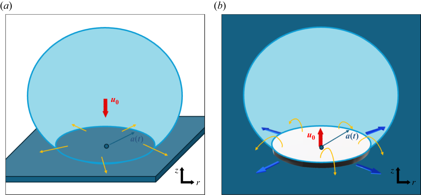


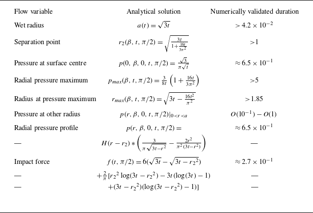


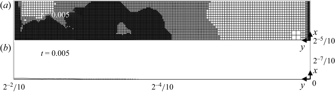


 Open access