2 Continuous action integral

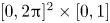
We will consider general mappings $\boldsymbol {x}(s, \theta, \zeta )$ between $(s, \theta, \zeta )$ with $s \in [0, 1]$, $\theta$, $\zeta \in [0, 2 {\rm \pi})$ and $\mathbb {R}^3$, analytic, and double periodic in $\theta$, and $\zeta$, $\boldsymbol {x}(s, \theta, \zeta ) = \boldsymbol {x}(s, \theta + 2{\rm \pi}, \zeta ) = \boldsymbol {x}(s, \theta, \zeta + 2 {\rm \pi})$. Boundary conditions are realised by providing a smooth toroidal external boundary $\boldsymbol {x}_b(\theta, \zeta )$ and by requiring that $\boldsymbol {x}(1, \theta, \zeta ) = \boldsymbol {x}_b(\theta, \zeta )$. A coordinate axis is defined as $\boldsymbol {x}_a(\zeta ) = \boldsymbol {x}(0, \theta, \zeta )$, demanding that the mapping continuously changes its topological structure from surfaces with $s \neq 0$ to a curve in space at $s = 0$. This condition creates a coordinate singularity at $\boldsymbol {x}_a$, since for fixed $\zeta$ every $\theta$ corresponds to the same point in real space, analogously to the polar coordinates. The objective of this work is to provide a construction of $\boldsymbol {x}$ such that it becomes a polar-like coordinate mapping, defined by having a non-vanishing coordinate Jacobian outside of the coordinate axis. Given such mapping $\boldsymbol {x}(s, \theta, \zeta )$, we can compute the covariant basis vectors $\boldsymbol {e}_s = \partial _s \boldsymbol {x}, \boldsymbol {e}_\theta = \partial _\theta \boldsymbol {x}, \boldsymbol {e}_\zeta = \partial _\zeta \boldsymbol {x}$, along with the corresponding metric elements $g_{ij} = \boldsymbol {e}_{i}\boldsymbol {\cdot }\boldsymbol {e}_j$ with $i,j = s, \theta, \zeta$. The Jacobian is given by $\sqrt {g} \equiv \boldsymbol {e}_s \boldsymbol {\cdot } (\boldsymbol {e}_\theta \times \boldsymbol {e}_\zeta )$. The Jacobian is defined up to a sign depending on whether the basis vectors form a right- or left-handed coordinate system. The contravariant basis vectors are $\boldsymbol {\nabla } s = \boldsymbol {e}_\theta \times \boldsymbol {e}_{\zeta }/\sqrt {g}$, $\boldsymbol {\nabla } \theta = \boldsymbol {e}_\zeta \times \boldsymbol {e}_{s}/\sqrt {g}$ and $\boldsymbol {\nabla } \zeta = \boldsymbol {e}_s \times \boldsymbol {e}_{\theta }/\sqrt {g}$. Considering different explicit forms of $\boldsymbol {x}$ in the space of mappings conforming to a boundary leads to different forms of the metric elements.

We now introduce a geometrical action $\mathcal {S}$ for the mapping $\boldsymbol {x}$ constrained to the boundary $\boldsymbol {x}_b$ as

(2.1)\begin{equation} \mathcal{S}[\boldsymbol{x}] = \int_0^{2{\rm \pi}}{\rm d}\zeta \int_{0}^{2{\rm \pi}}{\rm d}\theta \int_{0}^1 {\rm d}s\left( \frac{1}{2} f \sqrt{g}^2 + \omega \sqrt{\boldsymbol{e}_s \boldsymbol{\cdot} \boldsymbol{e}_s}\right). \end{equation}

Here, $f(\boldsymbol {x}; s, \theta, \zeta )$ is a positive function of the mapping and it can explicitly depend on $(s, \theta, \zeta )$. As discussed in § 3, $f$ can be used for fixing the functional form of $\sqrt {g}$. A specific form for $f$ given below is chosen to recover the simple case of circular cross-section axisymmetric torus to ensure the polar-like property of $\boldsymbol {x}$. The parameter $\omega$ is a constant weighting coefficient. We assert that the minimum of $\mathcal {S}$ in the space of mappings maximises the set of points in coordinate space where the Jacobian is non-zero.

The corresponding Lagrangian $\mathcal {L} = \frac {1}{2} f \sqrt {g}^2 + \omega \sqrt {\boldsymbol {e}_s \boldsymbol {\cdot }\boldsymbol {e}_s}$ encodes the key geometrical insights that lead to the desired coordinate mapping property. From the analyticity of $\boldsymbol {x}$, for having $\sqrt {g} \neq 0$, it is crucial for the Jacobian to have a uniform sign. Considering that the overall volume $\mathcal {V} = \int {\rm d}\zeta \,{\rm d}\theta \,{\rm d}s \,\sqrt {g}$ is independent of the mapping, if $\sqrt {g}$ was decreasing up to becoming negative in a given subset of volume, it must increase somewhere else to counteract the effect, therefore leaving $\mathcal {V}$ constant. Having regions of negative $\sqrt {g}$ and positive $\sqrt {g}$ necessarily leads to larger integrated values of $\sqrt {g}^2$, since there are competing parts of the volume integrand. Moreover, the minimisation of $\sqrt {g}^2$ smooths the regions where $\sqrt {g}$ has a peak in its amplitude. Due to volume conservation, the gradients near the regions where the Jacobian is changing sign get weakened up to the point where it reaches homogeneity in sign.

Adding $\omega \sqrt {\boldsymbol {e}_s \boldsymbol {\cdot } \boldsymbol {e}_s}$ to the action serves to penalise curvature in the radial coordinate lines, and thus increasing $\omega$ leads to coordinate mappings with straighter coordinate lines. This contribution to the action was found to be required after an initial numerical exploration suggested that, otherwise, the action functional would be independent of the parametrisation in the poloidal angle coordinate. The proportionality to $\sqrt {g}^2$, represented by $f$, needs to have the same sign of $\omega$ for not introducing any competition between having a constant sign for $\sqrt {g}$ and the straightness of coordinate lines. By conventionally choosing to minimise $\mathcal {S}$, we impose $f$ and $\omega$ to be both positive.

Note that there are multiple ways to include the boundary constraint $\boldsymbol {x}(1, \theta, \zeta ) = \boldsymbol {x}_{b}(\theta, \zeta )$, e.g. by introducing a Lagrange multiplier $\lambda (\theta, \zeta )$ in $\mathcal {S}$ via the addition of the term

(2.2)\begin{equation} \int_0^{2{\rm \pi}}{\rm d}\zeta \int_{0}^{2{\rm \pi}}{\rm d}\theta \lambda(\theta, \zeta)|\boldsymbol{x}(1, \theta, \zeta) - \boldsymbol{x}_b(\theta, \zeta)|. \end{equation}

3 Euler–Lagrange equations

In the variational approach, $\boldsymbol {x}$ constitutes the dynamic variable independent from $(s, \theta, \zeta )$. The relation between $\boldsymbol {x}$ and $(s, \theta, \zeta )$, i.e. the mapping, is recovered by solving the EL equations, analogously to the Lagrangian approach in classical mechanics. We can compute the stationary points in the action $\mathcal {S}$ in (2.1) by considering the variation of the coordinate mapping $\delta \boldsymbol {x} \equiv \boldsymbol {x} - \boldsymbol {x}^{\prime }$, where $\boldsymbol {x}$ and $\boldsymbol {x}^{\prime }$ are two independent mappings constrained to $\boldsymbol {x}_b$. The boundary conditions fix the possible mapping variations at the external surface, $\delta \boldsymbol {x}(1, \theta, \zeta ) = \delta \boldsymbol {x}_b(\theta, \zeta ) = 0$; and at the coordinate axis, $\delta \boldsymbol {x}(0, \theta, \zeta )$ = $\delta \boldsymbol {x}(\zeta )$. The variation of the action in (2.1) with respect to the coordinate mapping $\boldsymbol {x}(s, \theta, \zeta )$ yields the EL equations

(3.1)\begin{equation} \boldsymbol{\nabla} (f \sqrt{g}) - \frac{\sqrt{g}}{2} \frac{\delta f}{\delta \boldsymbol{x}} + \frac{\omega}{\sqrt{g}}\boldsymbol{\kappa}= 0, \end{equation}

having defined the curvature vector as $\boldsymbol {\kappa } = \partial _s (\boldsymbol {e}_s / |\boldsymbol {e}_s|)$. It accounts for the variation of the tangential lines along the radial direction, being a measure of the straightness of $\theta,\zeta ={\rm const}$. coordinate lines. The EL equations are a set of nonlinear partial differential equations with boundary conditions. Their derivation is presented in Appendix A. The first term on the left of (3.1) accounts for the volume element compared with a Jacobian that would scale as $1/f$. The second term is the contribution from the variation of $f$ with respect to $\boldsymbol {x}$. Lastly, the curvature term represented by $\boldsymbol {\kappa }$ and weighted by $\omega$, quantifies deviations from straight radial lines.

The function $f$ can be either externally prescribed or determined by solving (3.1) for a specific choice of $\boldsymbol {x}$. To fix $f$, we impose that the known analytical mapping of a torus with a circular cross-section is recovered exactly by the action minimisation when $\omega$ = 0. The analytical mapping reads as $\boldsymbol {x} = R \, \hat {\boldsymbol {R}} + Z \boldsymbol {e}_z$, with $\hat {\boldsymbol {R}} = (\cos \phi \boldsymbol {e}_x + \sin \phi \boldsymbol {e}_y)$, $\boldsymbol {e}_x, \boldsymbol {e}_y, \boldsymbol {e}_z$ unitary Cartesian vectors, and $R = 1 + s \cos (\theta ),Z=s\sin (\theta )$, with $\theta$ representing the geometrical poloidal angle. For applying the variation approach, we note that, in general, $R$ depends on the coordinate mapping $\boldsymbol {x}$ and, implicitly on $s, \theta, \zeta$. By choosing

(3.2)\begin{equation} f = 1/[s \, R^2(\boldsymbol{x}, s, \theta, \zeta)], \end{equation}

we have $\delta f/ \delta \boldsymbol {x} = - ({2}/{s R^3})\hat {\boldsymbol {R}}$. Substituting this expression into (3.1), the EL equations are trivially satisfied, as intended. Therefore, if $f$ is taken as in (3.2) with a circular torus given as a boundary, the minimisation of the action integral will recover the analytic mapping. Given the topological equivalence of toroidal domains with a torus with a circular cross-section, we choose (3.2) to define $f$ for the following analysis.

4 Numerical implementation

4.1 Zernike–Fourier representation

We consider the local form for the mapping as $\boldsymbol {x} = R(\boldsymbol {x}, s, \theta, \zeta )\,\hat {\boldsymbol {R}} + Z(\boldsymbol {x}, s, \theta, \zeta )\, \boldsymbol {e}_z$. The Jacobian is computed as: $\sqrt {g} = R \sqrt {g}_p = R (\partial _s R \partial _\theta Z - \partial _s Z \partial _\theta R)$, where $\sqrt {g}_p$ is the poloidal part of the Jacobian. The metric elements are $g_{ij} = \partial _i R \partial _j Z + \partial _j R \partial _i Z + \delta _{i\zeta } R^2$, where $\delta _{i\zeta } = 1$ if $i = \zeta$ and $0$ otherwise. In addition to considering double-periodic mappings, we impose stellarator symmetry (Lee et al. Reference Lee, Harris, Hirshman and Neilson1988) to simplify the computations. This discrete symmetry is defined as $R(s, -\theta, -\zeta ) = R(s, \theta, \zeta )$ and $Z(s, -\theta, -\zeta ) = -Z(s, \theta, \zeta )$, which implies a more general symmetry (Dewar & Hudson Reference Dewar and Hudson1998). Stellarators are typically composed of a number of identical sectors $N_{P}$, called field periods. A double-periodic function $h(s, \theta, \zeta )$ can be expressed in a Fourier–Zernike (McAlinden, McCartney & Moore Reference McAlinden, McCartney and Moore2011) basis as

(4.1)\begin{align} h(s, \theta, \zeta) & = \sum_{n = 0}^{+ \infty}\sum_{l = 0}^{+ \infty}\sum_{m = 0}^{l}\left[\left( C_{+, nlm}\mathcal{Z}^{m}_l(s, \theta) + C_{-, nlm}\mathcal{Z}^{{-}m}_l(s, \theta) \right)\cos(n N_{P} \zeta) \right.\nonumber\\ & \quad \left. + \left(S_{+, {nlm}}\mathcal{Z}^{m}_l(s, \theta) + S_{-, {nlm}}\mathcal{Z}^{{-}m}_l(s, \theta) \right)\sin(n N_{P} \zeta)\right], \end{align}

where the Zernike polynomials (Niu & Tian Reference Niu and Tian2022) are given as $\mathcal {Z}^{m}_l = \mathcal {R}^m_l \cos (m \theta )$ and $\mathcal {Z}^{-m}_l = \mathcal {R}^m_l \sin (m \theta )$, with radial part

(4.2)\begin{equation} \mathcal{R}^m_l(s) = \begin{cases} \sum\limits_{k = 0}^{({l - m})/{2}} \dfrac{(- 1)^k(l - k)!}{k!\left(\dfrac{l + m}{2}- k\right)! \left(\dfrac{l - m}{2} - k\right)!} s^{l - 2k}, & l - m \ \text{even} \\[10pt] 0 , & l - m \ \text{odd}, \end{cases} \end{equation}

for $l\geqslant m$, with $n,l,m \in \mathbb {N}^{+}$. The real coefficients $C_{+, {nlm}}, C_{-,{nlm}}, S_{+, {nlm}}, S_{-, {nlm}}$ parametrise the mapping in the Fourier–Zernike space. The Zernike polynomials are orthogonal basis functions on the unit disk, and they can describe the mapping with half of the coefficients used by the parity-restricted Chebyshev polynomials (Mason & Handscomb Reference Mason and Handscomb2002) often used in plasma physics. The normalisation is chosen such that the inner product $\langle A B \rangle = \int _0^1 \int _{0}^{2{\rm \pi} } A(s, \theta ) B(s, \theta ) s \,{\rm d}s\,{\rm d}\theta$ defined on the space of $\mathcal {L}^2$ functions on the disk gives

(4.3)\begin{equation} \langle\mathcal{Z}^m_l \mathcal{Z}^{m'}_{l'} \rangle = \frac{1 + \delta_{m0}}{2(l + 1)} \delta_{m m'} \delta_{l l'}. \end{equation}

Stellarator symmetry imposes $\mathcal {C}_{-, {nlm}} = \mathcal {S}_{+, {nlm}} = 0$ for $R$ and $\mathcal {C}_{+, {nlm}}= \mathcal {S}_{-, {nlm}} = 0$ for $Z$. Extending the sum to negative values of $n$, and redefining the set of Fourier–Zernike coefficients in terms of $r_{nlm}, z_{nlm}$ and $n \in \mathbb {Z}$, the discretised mapping becomes(Qu et al. Reference Qu, Pfefferlé, Hudson, Baillod, Kumar, Dewar and Hole2020)

(4.4)\begin{gather} R(s, \theta, \zeta) = \sum_{n ={-}N}^{N}\sum_{m = 0}^{M}\sum_{m = l}^{L} r_{nlm} \mathcal{R}^m_l(s)\cos(m \theta - n N_{P} \zeta), \end{gather}

(4.5)\begin{gather}Z(s, \theta, \zeta) = \sum_{n ={-}N}^{N}\sum_{m = 0}^{M}\sum_{m = l}^{L} z_{nlm} \mathcal{R}^m_l(s)\sin(m \theta - n N_{P} \zeta), \end{gather}

where $N$, $M$ and $L \in \mathbb {N}^{+}$ indicate the resolution imposed in the Fourier–Zernike space. The number of components in $r_{nlm}$ and $z_{nlm}$ scales as $2 M^2 N$. The Fourier–Zernike mapping in the poloidal plane directly satisfies the condition to be analytic (Boyd & Yu Reference Boyd and Yu2011) since the radial part with poloidal mode number $m$ scales as $\mathcal {R}^m_l(s) \sim s^m(\mathcal {R}^{m}_{0} + \mathcal {R}^m_2 s^2 + \mathcal {R}^m_4 s^4 + \dots )$. Therefore, no special treatment in terms of coordinate regularisation is required for the coordinate axis, where the coordinate mapping will be polar-like at the leading order. The boundary surface $\boldsymbol {x}_b(\theta, \zeta )$ is given in terms of its Fourier components

(4.6)\begin{gather} R^b(\theta, \zeta) = \sum_{n ={-}N_b}^{N_b}\sum_{m = 0}^{M_b} R^b_{nm} \cos(m\theta - N_{P} n \zeta), \end{gather}

(4.7)\begin{gather}Z^b(\theta, \zeta) = \sum_{n ={-}N_b}^{N_b}\sum_{m = 0}^{M_b} Z^b_{nm} \sin(m\theta - N_{P} n \zeta), \end{gather}

where $N_b, M_b \in \mathbb {N}^{+}$ are the prescribed toroidal and poloidal boundary resolutions. In the following, we consider $M= L$. The boundary condition $\boldsymbol {x}(1, \theta, \zeta ) = \boldsymbol {x}_{b}(\theta, \zeta )$ reduces the number of independent components in $r_{nlm}$ and $z_{nlm}$. Using the property for the Zernike radial part of $\mathcal {R}_l^m(1) = 1$ for each $m,l$, the explicit form for the boundary condition becomes

(4.8a)\begin{equation} \sum_{l = m}^{L}r_{nlm} = R^b_{nm} , \quad \sum_{l = m}^{L}z_{nlm} = Z^b_{nm}. \end{equation}

These equations are exploited to fix $(M + 1)(2N + 1)$ components of $r_{nlm}$ and $z_{nlm}$. The coefficients $r_{nmm}$ and $z_{nmm}$ for each $n$ and $m$ are indeed fixed as $r_{nmm} = R^{b}_{nm} - \sum _{l = m + 1}^{L}r_{nlm}$, $z_{nmm} = Z^{b}_{nm} - \sum _{l = m + 1}^{L}z_{nlm}$.

4.2 Action discretisation

Instead of directly using the Zernike–Fourier representation of the mapping in (2.1), exploiting a coordinate grid highlights the geometrical properties of $\mathcal {S}$ in terms of areas and radial lengths. The idea is depicted in the illustration provided in figure 3.

Figure 3.

Schematic illustration of the geometrical elements in the action discretisation.

As drawn under $(a)$, starting with a grid $\{s_i, \theta _j, \zeta _k\}$ in coordinate space with $i \in [0, N_s]$, $j \in [0, N_\theta ]$ and $k \in [0, N_{\zeta }]$, $\boldsymbol {x}$ maps the corresponding points into a grid of $R_{ijk}$ and $Z_{ijk}$. Fixing a toroidal angle $\zeta _k$, the grid in the poloidal plane is illustrated in figure 3(b). Connecting the points with straight lines along the coordinate lines we have a set of quadrilaterals and triangles. Each of them has an area $\mathcal {A}_{ijk}$ constituted by the grid points $\boldsymbol {x}_{ijk}$, $\boldsymbol {x}_{i + {1 j k}}$, $\boldsymbol {x}_{i + 1 j+1 k}$ and $\boldsymbol {x}_{i j+1 k}$. At the coordinate axis, for which $i = 0$, we have that $\boldsymbol {x}_{0 j+1 k} = \boldsymbol {x}_{0 j k}$. The expression of $\mathcal {A}_{ijk}$ is explicitly given by the Shoelace formula (Braden Reference Braden1986). Each point $\boldsymbol {x}_{ijk}$ identifies a radial length $L_{ijk}$ to $\boldsymbol {x}_{i+1jk}$ via the Euclidean distance of two points. The convention assumed for the identification of each grid point in $\mathcal {A}_{ijk}$ and in $L_{ijk}$ is shown in figure 3. Given a point $\boldsymbol {x}_{ijk}$ the points at $i + 1$ and $j + 1$ correspond to the incremental radial and poloidal coordinates, respectively. For this reason, $\mathcal {A}_{ijk}$ and $L_{ijk}$ are not defined at the boundary.

By choosing $f$ following (3.2), the Jacobian reduces to a poloidal Jacobian, such that $f \sqrt {g}^2 = \sqrt {g}_p^2/s$. Thus, the discrete action integral can be computed as

(4.9)\begin{equation} \mathcal{S}[\boldsymbol{x}_{ijk}] = \sum_{ijk}\left(\frac{1}{2 s_i} \mathcal{A}^2_{ijk} + \omega L_{ijk}\right), \end{equation}

where we approximated the poloidal Jacobian with the area element, considered an equispaced grid, and neglected common multiplicative factors. Here, $\mathcal {S}[\boldsymbol {x}_{ijk}]$ is an explicit function in terms of the free variables $\{r_{nlm}, z_{nlm}\}$. Minimising $\mathcal {S}$ is an unconstrained nonlinear optimisation problem that we solve using the Broyden–Fletcher–Goldfarb–Shanno algorithm (Dai Reference Dai2002), a descent-gradient iterative method with an explicit computation of the gradient in the space of free parameters as illustrated in Appendix F.

6 GVEC application

The approach of minimising the action functional (A5) is successfully tested in GVEC (Hindenlang et al. Reference Hindenlang, Maj, Strumberger, Rampp and Sonnendrücker2019), a 3-D MHD equilibrium solver assuming closed nested flux surfaces. In GVEC, the flux surface coordinate mapping $R(s,\theta,\zeta ), Z(s,\theta,\zeta )$ is discretised by a tensor product of B-splines in $s$ and Fourier modes in angular directions. Using a $1$ element B-spline of degree equal to the maximum poloidal mode number, and smoothness constraints at the axis, the Zernike–Fourier representation is exactly recovered. As a 3-D test case, a W7-X-like boundary with an initial circular magnetic axis was taken, where the usual initialisation of GVEC produces an initial state with regions having $\sqrt {g} < 0$, as shown in figure 10(a). The maximum Jacobian used for the normalisation is always positive.

Figure 10.

GVEC results for the minimisation of the action functional (A5) using a 3-D W7-X-like boundary and a circular axis for initialisation. The normalised scaled Jacobian is shown in colour, along with the $(s,\theta )$ grid for 4 poloidal cross-sections. The mapping is discretised with a Zernike–Fourier representation, using $1$ B-spline element in the radial direction and $(m,n)_\textrm {max}=7$. (a) Initial state with $\sqrt {g}<0$. (b–d) Valid optimised grids for increasing weighting factor $\omega$. Note that $\max (\sqrt {g})$ is always positive.

The minimisation of $\mathcal {S}$ with a gradient descent successfully produced $\sqrt {g}>0$. This is shown in figures 10(b), 10(c) and 10(d), where the initial invalid $(s,\theta )$ grid and final valid grids for different weighting factors $\omega$ are shown, as well as the normalised scaled Jacobian.

The free parameter $\omega >0$ acts as a penalty term in the minimisation, increasing the straightness of $\theta$ contours, but its maximum value is not known a priori. The strength of $\omega$ is a trade-off between the straightness of the $\theta$-contours, the axis position and consequently also the minimal scaled Jacobian. As seen in figures 10(b)–10(d), for increasing $\omega$, the $\theta$-contours are straightened, at the cost of a smaller minimal Jacobian, being close to zero for $\omega =0.8$. In $(b)$, $\omega =0.01$ leads to a slightly oscillating behaviour of the $\theta$-contours. Using these solutions as initialisation for the MHD energy minimisation, it was found that GVEC had no difficulties converging to an equilibrium for moderate $\omega \leqslant 0.2$.