


1. Introduction
In experimental and numerical studies, the flow information is usually only partially available due to technical limitations in measuring sensors or the inaccuracy of the numerical models. For numerical studies, the popular wall-modelled large-eddy simulation (WMLES), which resolves only the large-scale motions beyond the local grid scale while modelling the near-wall small-scale motions with the wall models (Larsson et al. Reference Larsson, Kawai, Bodart and Bermejo-Moreno2016; Fu et al. Reference Fu, Karp, Bose, Moin and Urzay2021; Fu, Bose & Moin Reference Fu, Bose and Moin2022; Griffin, Fu & Moin Reference Griffin, Fu and Moin2023), achieves a good balance between the computational cost and accuracy. However, the near-wall dynamics, as an important turbulence property, is usually inaccurately evaluated by the WMLES (Bae et al. Reference Bae, Lozano-Durán, Bose and Moin2018). On the other hand, the spatial and temporal resolutions of the experimental results are usually restricted by the limitations in the measuring equipment (Nobach & Bodenschatz Reference Nobach and Bodenschatz2009; Cameron Reference Cameron2011). Current attempts to estimate the missing dynamics of turbulence can be categorised into the data-driven approaches (Marusic, Mathis & Hutchins Reference Marusic, Mathis and Hutchins2010; Baars, Hutchins & Marusic Reference Baars, Hutchins and Marusic2016; Guastoni et al. Reference Guastoni, Güemes, Ianiro, Discetti, Schlatter, Azizpour and Vinuesa2021) and the physics-based ones (Chevalier et al. Reference Chevalier, Hœpffner, Bewley and Henningson2006; Hwang & Cossu Reference Hwang and Cossu2010; McKeon & Sharma Reference McKeon and Sharma2010; Martini et al. Reference Martini, Cavalieri, Jordan, Towne and Lesshafft2020; Towne, Lozano-Durán & Yang Reference Towne, Lozano-Durán and Yang2020).
The data-driven approaches estimate the flow field with the knowledge obtained from the existing flow data. The well-known attached-eddy model (AEM) (Townsend Reference Townsend1976) and the inner–outer interaction model (IOIM) (Marusic et al. Reference Marusic, Mathis and Hutchins2010; Baars et al. Reference Baars, Hutchins and Marusic2016) that describe the flow motions in turbulence are proposed based on extensive observation and investigation on the wall-bounded turbulence. According to the IOIM, the large-scale motions (LSMs) and very-large-scale motions (VLSMs) influence the near-wall turbulence through the superposition and modulation effects. Specifically, the superposition effects of the LSMs and VLSMs on near-wall motions can be determined through the transfer kernel estimated from the cross-spectral density (CSD) tensor, which builds up the linear relationship between the flow motions at different wall-normal locations (Gupta et al. Reference Gupta, Madhusudanan, Wan, Illingworth and Juniper2021). It can be demonstrated that the superposition effect defined by the IOIM corresponds to the optimal linear estimation with the knowledge of the spatial cross-spectra of the streamwise velocity. The consistency between the AEM and IOIM has been demonstrated in Cheng & Fu (Reference Cheng and Fu2022), which is then used to study the isolated attached eddies with a give scale (Cheng, Shyy & Fu Reference Cheng, Shyy and Fu2022). Besides the traditional data-driven approaches that use predefined transfer functions, the deep neural networks and convolutional neural networks (CNNs) are used for the prediction of the flow system in a nonlinear manner (e.g. Lozano-Durán, Bae & Encinar Reference Lozano-Durán, Bae and Encinar2020; Guastoni et al. Reference Guastoni, Güemes, Ianiro, Discetti, Schlatter, Azizpour and Vinuesa2021). Guastoni et al. (Reference Guastoni, Güemes, Ianiro, Discetti, Schlatter, Azizpour and Vinuesa2021) predicts the wall-bounded turbulence from the wall measurements with the CNNs using a linear combination of orthonormal basis functions obtained from proper orthogonal decomposition, which improves the prediction accuracy at large wall-normal distances compared with that from the CNN that directly predicts the turbulent motions.
The physics-driven approaches estimate the flow field based on the Navier–Stokes (NS) equations that govern the flow dynamics. The NS equations can be rearranged into the form of the linearised relationship between the nonlinear forcing (input) and the response of the velocity, pressure and temperature (output) (Hwang & Cossu Reference Hwang and Cossu2010; McKeon & Sharma Reference McKeon and Sharma2010). When the linear relationship is built between the forcing and response in the frequency domain, the corresponding linear operator is named the resolvent (McKeon & Sharma Reference McKeon and Sharma2010). The resolvent analysis usually focuses on uncovering the coherence properties of turbulence through mathematical investigations on the resolvent operator. Through the singular value decomposition of the resolvent operator, the normalised forcing and response modes ordered by their gains are obtained. Specifically, when the gain of the leading mode is much larger than the sequential modes, the corresponding response mode could be considered to dominate the resultant response. The domination of the leading resolvent response mode over the sequential ones is denoted as low-rank behaviour (Pickering et al. Reference Pickering, Rigas, Schmidt, Sipp and Colonius2021). Assuming low-rank behaviour, the leading response mode at a given spatio-temporal scale can be regarded as the representative flow pattern at such a scale. Such simplification achieves large success in qualitatively describing the coherent structures of turbulence with only the mean velocity profile obtained from the direct numerical simulation (DNS) (McKeon & Sharma Reference McKeon and Sharma2010; Moarref et al. Reference Moarref, Sharma, Tropp and McKeon2013) or the ordinary differential equation solvers (Hwang & Cossu Reference Hwang and Cossu2010; Chen et al. Reference Chen, Cheng, Fu and Gan2023a,Reference Chen, Cheng, Gan and Fub). However, the actual response of the flow dynamic system is determined by, not only the response modes and gains, but also the variations of forcing projections on different resolvent forcing modes, which cannot be ignored for the energy-containing flow scales (Morra et al. Reference Morra, Semeraro, Henningson and Cossu2019, Reference Morra, Nogueira, Cavalieri and Henningson2021). Thus, for the flow state estimation in this study, where higher accuracy is needed, the low-rank behaviour is not suitable to directly utilise.
Besides the approaches utilising the low-rank behaviour of the resolvent operator, the modelling of the input forcing is also broadly investigated for the prediction of the flow statistics (Madhusudanan, Illingworth & Marusic Reference Madhusudanan, Illingworth and Marusic2019; Morra et al. Reference Morra, Semeraro, Henningson and Cossu2019; Gupta et al. Reference Gupta, Madhusudanan, Wan, Illingworth and Juniper2021; Ying et al. Reference Ying, Liang, Li and Fu2023). By modelling a part of the forcing with the eddy-viscosity model (Cess Reference Cess1958; Reynolds & Hussain Reference Reynolds and Hussain1972) while considering the remaining part of the forcing to be white in space, the predicted accuracy of the energy profile of the response is much improved (Hwang & Cossu Reference Hwang and Cossu2010; Morra et al. Reference Morra, Semeraro, Henningson and Cossu2019). Later, with the cross-spectra predicted by such eddy-viscosity-modelled forcing, Madhusudanan et al. (Reference Madhusudanan, Illingworth and Marusic2019) estimate the large-scale structures of the turbulent channel flow via the linear stochastic estimation. Compared with the ones without the eddy-viscosity model, the predicted energy spectra and large-scale structures from the modelled forcing match much better with the DNS results (Madhusudanan et al. Reference Madhusudanan, Illingworth and Marusic2019), which demonstrates the importance of the forcing model in turbulent estimation in cases where the real forcing statistics are unavailable. Gupta et al. (Reference Gupta, Madhusudanan, Wan, Illingworth and Juniper2021) further improve the estimation accuracy by introducing additional forcing models that consider the variation of the stochastic forcing profile with heights and flow scales, namely the W-model and  $\lambda$-model. The W-model and $\lambda$-model are demonstrated to further improve the prediction accuracy of the linear coherence spectrum and the large-scale flow structures. Ying et al. (Reference Ying, Liang, Li and Fu2023) propose the resolvent-informed white-noise-based estimation (RWE) approach to model the remaining part of the forcing by modifying the initially white forcing according to the estimated near-wall energy profile based on resolvent-based estimation (RBE) that will be introduced in the following. With input data of the mean velocity profile and temporally resolved measurement data, the RWE provides an accurate prediction of the turbulence statistics, including the energy spectra, space–time correlation and large-scale structures in the near-wall region.
The above-introduced forcing models focus on the prediction of the flow statistics. On the other hand, it is also very important to estimate the instantaneous flow state with the measured flow state. The predicted flow statistics from the forcing models can be used to inform the estimators of the fluctuation flow state, as will be illustrated in the following. The physics-based approaches for state estimation of the dynamic system include the Kalman-filter-based approaches (Kalman Reference Kalman1960; Hœpffner et al. Reference Hœpffner, Chevalier, Bewley and Henningson2005; Chevalier et al. Reference Chevalier, Hœpffner, Bewley and Henningson2006; Colburn, Cessna & Bewley Reference Colburn, Cessna and Bewley2011), the  $H_2$-optimal control approach (Illingworth, Monty & Marusic Reference Illingworth, Monty and Marusic2018) and the resolvent-based approaches (Martini et al. Reference Martini, Cavalieri, Jordan, Towne and Lesshafft2020; Towne et al. Reference Towne, Lozano-Durán and Yang2020; Amaral et al. Reference Amaral, Cavalieri, Martini, Jordan and Towne2021). The Kalman filter (Kalman Reference Kalman1960) includes a set of recursive algorithms that estimate the flow state with the knowledge of the statistics of the stochastic input forcing and measurement noise, which are both assumed to be white in time. To estimate the flow state at the current time step, the causal Kalman filter includes two phases, namely the prediction phase and the update phase. In the prediction phase, the current state is predicted from the state estimation at the previous time step. Then, the prediction is modified by minimising the expected estimation error covariance according to the current noise-containing measurements in the update phase. For non-causal cases, the so-called Kalman smoother further corrects the estimation at a given time step with later measurements. Regardless of whether the stochastic input and measurement noise are Gaussian, the Kalman filter could provide the optimal linear estimation in the minimum mean square error (MSE) sense (Humpherys, Redd & West Reference Humpherys, Redd and West2012). When applied in turbulence estimation, it is crucial to appropriately model the temporal evolution of the input forcing to ensure the prediction accuracy of the Kalman filter. The early Kalman-filter-based studies in turbulence estimation (Hœpffner et al. Reference Hœpffner, Chevalier, Bewley and Henningson2005; Chevalier et al. Reference Chevalier, Hœpffner, Bewley and Henningson2006) assume that the forcing is white in time, which cannot model well the real forcing that is coloured in time (Zare, Jovanović & Georgiou Reference Zare, Jovanović and Georgiou2017; Zare, Georgiou & Jovanović Reference Zare, Georgiou and Jovanović2020). Zare et al. (Reference Zare, Chen, Jovanović and Georgiou2016) propose a stochastic modelling approach that generates a coloured-in-time forcing sequence from the knowledge of the spatial spectra of response along the height, which can potentially enhance the effectiveness of the Kalman filter by introducing that coloured forcing. However, the current stochastic dynamical modelling approach cannot well reproduce the energy distribution of forcing in the frequency domain (Zare et al. Reference Zare, Georgiou and Jovanović2020), which needs further exploration. On the other hand, the $H_2$-optimal control approach (Doyle et al. Reference Doyle, Glover, Khargonekar and Francis1989) constructs a rational controller that minimises the $H_2$ norm of the transfer matrix that links the external input and the estimation error when this approach is used for causal state estimation. The $H_2$-optimal control approach assumes that the forcing and measurement noise are both white in time, which is the optimal linear causal estimator when the spatial covariance of the external forcing is known. Illingworth et al. (Reference Illingworth, Monty and Marusic2018) utilise the $H_2$-optimal control approach in estimating the large-scale structures in turbulent channel flow using the measurements at the logarithmic region.
The RBE (Martini et al. Reference Martini, Cavalieri, Jordan, Towne and Lesshafft2020; Towne et al. Reference Towne, Lozano-Durán and Yang2020; Amaral et al. Reference Amaral, Cavalieri, Martini, Jordan and Towne2021) estimates the flow state in the frequency domain, which can be regarded as the multiple-input and multiple-output (MIMO) Wiener filter (Wiener Reference Wiener1930, Reference Wiener1949). The RBE is initially proposed by Towne et al. (Reference Towne, Lozano-Durán and Yang2020), which estimates the input forcing of the dynamic system by finding the minimum  $L^2$-norm solution that reproduces the measurements. Here, the $L^2$ norm is defined as the inner product of a vector. Later, Martini et al. (Reference Martini, Cavalieri, Jordan, Towne and Lesshafft2020) improve the RBE, which enables the incorporation of the forcing models. The linear estimator of the improved RBE can be constructed by searching for the stationary point of the expected CSD tensor of the estimation error. In this sense, the original RBE by Towne et al. (Reference Towne, Lozano-Durán and Yang2020) can be regarded as the one that finds the stationary point of the error CSD tensor assuming that the forcing is uniform and uncorrelated in space. With the improved RBE informed by the real forcing statistics, Amaral et al. (Reference Amaral, Cavalieri, Martini, Jordan and Towne2021) estimate the flow state of turbulent channel flow with the measurements of wall shear stress and pressure.
Although the RBE has the desirable property of minimising the generic error norm, it has a high requirement on the spatio-temporal resolutions of the measurement. In practice, temporally resolved data could be unavailable due to the high computational and storage costs in numerical studies or the equipment limitations in experiments. For high Reynolds number turbulence, the temporally resolved DNS data could hardly be stored due to the huge storage cost, which hinders the validation and application of the resolvent-based approaches in such cases. Meanwhile, in numerical or experimental studies, some snapshots might become unavailable due to the corruption of the digital storage device or the failure of the measuring equipment. Thus, an estimator that enables arbitrary sampling time intervals is needed for the flow estimations in such cases with unresolved-in-time measurement data. In this study, a generalised version of the RBE will be proposed, which enables physics-based estimation using the measured data with arbitrary time intervals. By incorporating the spatio-temporal forcing statistics or forcing models, the new approach constructs the linear estimator by finding the stationary points of the spatio-temporal covariance tensor of the estimation error. When the real forcing and noise statistics are incorporated into the estimator, the optimal linear estimation can be obtained with the given temporal resolution of the measurements.
The remainder of this article is organised as follows. In § 2, the generalised resolvent-based estimator (GRBE) approach is derived based on the linearised NS equations. In § 3, the newly proposed method is validated for the complex Ginzburg–Landau equation and turbulent channel flows. In § 4, the new approach is utilised to investigate the impacts of different measuring conditions and the incorporation of forcing models on the estimation accuracy. Discussions and concluding remarks are presented in § 5.
2. Methodology
In this section, the linearisation of the incompressible NS equations that govern the dynamics of turbulence is described, followed by the introduction of the resolvent analysis. Then, the derivation and discussions of the newly proposed GRBE will be presented.
2.1. Linearisation of the incompressible Navier–Stokes equations
The incompressible NS equations are given by
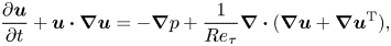 $$\begin{gather} \frac{\partial \boldsymbol{u}}{\partial t}+\boldsymbol{u}\boldsymbol{\cdot}\boldsymbol{\nabla}\boldsymbol{u} ={-}\boldsymbol{\nabla} p+\frac{1}{Re_\tau}\boldsymbol{\nabla}\boldsymbol{\cdot}(\boldsymbol{\nabla} \boldsymbol{u}+\boldsymbol{\nabla}\boldsymbol{u}^{\rm T}), \end{gather}$$
 $$\begin{gather}\boldsymbol{\nabla}\boldsymbol{\cdot}\boldsymbol{u} = 0, \end{gather}$$
where  $Re_\tau = {u_{\tau } h}/{\nu }$ is the friction Reynolds number, $u_{\tau }$ is the friction velocity, $h$ is the half-channel width, $\nu$ is the kinetic viscosity and the superscript ${}^{\rm T}$ denotes transpose. The linearised NS equations with respect to the fluctuation velocity $\boldsymbol {u}^{\prime }$ and pressure $p^{\prime }$ are expressed by
 $$\begin{gather} \frac{\partial \boldsymbol{u}^\prime}{\partial t}+\boldsymbol{U} \boldsymbol{\cdot}\boldsymbol{\nabla}\boldsymbol{u}^\prime +\boldsymbol{u}^\prime\boldsymbol{\cdot}\boldsymbol{\nabla} \boldsymbol{U}+\boldsymbol{\nabla} p^\prime -\frac{1}{Re_\tau}\boldsymbol{\nabla}\boldsymbol{\cdot} (\boldsymbol{\nabla}\boldsymbol{u}^\prime+{\boldsymbol{\nabla}\boldsymbol{u}^\prime}^{\rm T}) = \boldsymbol{f}_0^{\prime}, \end{gather}$$
 $$\begin{gather}\boldsymbol{\nabla}\boldsymbol{\cdot}\boldsymbol{u}^\prime = 0, \end{gather}$$
where  ${}^\prime$ denotes the fluctuation variable, $U$ is the mean velocity and the nonlinear forcing term is defined as
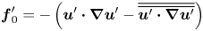 \begin{equation} \boldsymbol{f}_0^{\prime} ={-} \left( \boldsymbol{u}^\prime\boldsymbol{\cdot}\boldsymbol{\nabla}\boldsymbol{u}^\prime - \overline{\overline{\boldsymbol{u}^\prime\boldsymbol{\cdot}\boldsymbol{\nabla}\boldsymbol{u}^\prime}}\right) \end{equation}
with the double overlines denoting the averaged value along the temporal and uniform spatial directions.
On the other hand, the nonlinear term on the right-hand side of (2.2) can be further decomposed into two parts, i.e. the eddy-viscosity terms that are linear functions of  $\boldsymbol {u}^{\prime }$ and the forcing $\boldsymbol {f}^{\prime }$ (Illingworth et al. Reference Illingworth, Monty and Marusic2018; Morra et al. Reference Morra, Semeraro, Henningson and Cossu2019; Towne et al. Reference Towne, Lozano-Durán and Yang2020). The linearised NS equations considering the eddy-viscosity model are expressed by
 $$\begin{gather} \frac{\partial \boldsymbol{u}^\prime}{\partial t}+\boldsymbol{U}\boldsymbol{\cdot}\boldsymbol{\nabla}\boldsymbol{u}^\prime +\boldsymbol{u}^\prime\boldsymbol{\cdot}\boldsymbol{\nabla} \boldsymbol{U}+\boldsymbol{\nabla} p^\prime -\frac{1}{Re_\tau}\boldsymbol{\nabla}\boldsymbol{\cdot} \left[\frac{\nu_t+\nu}{\nu}(\boldsymbol{\nabla}\boldsymbol{u}^\prime+{\boldsymbol{\nabla}\boldsymbol{u}^\prime}^{\rm T})\right] = \boldsymbol{f}^{\prime}, \end{gather}$$
 $$\begin{gather}\boldsymbol{\nabla}\boldsymbol{\cdot}\boldsymbol{u}^\prime = 0, \end{gather}$$
where the forcing term is defined as
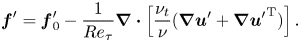 \begin{equation} \boldsymbol{f}^{\prime}= \boldsymbol{f}_0^{\prime} -\frac{1}{Re_\tau}\boldsymbol{\nabla}\boldsymbol{\cdot} \left[\frac{\nu_t}{\nu}(\boldsymbol{\nabla}\boldsymbol{u}^\prime+{\boldsymbol{\nabla}\boldsymbol{u}^\prime}^{\rm T})\right]. \end{equation}
The eddy viscosity  $\nu _t$ can be calculated from the semi-empirical expression of Cess (Reference Cess1958) as reported by Reynolds & Hussain (Reference Reynolds and Hussain1972)
 \begin{align}
\nu_t=\frac{\nu}{2} \left\{ 1+\frac{\kappa^2 Re_\tau ^2}{9} (2\tilde{y}-\tilde{y}^2)^2
(3-4\tilde{y}+2\tilde{y}^2)^2 \left[1-{\rm exp}\left(\frac{-Re_\tau (1-\left|1-\tilde{y}\right|)}{A}\right)\right]^2 \right\}^{1/2} -\frac{\nu}{2},
\end{align}
\begin{align}
\nu_t=\frac{\nu}{2} \left\{ 1+\frac{\kappa^2 Re_\tau ^2}{9} (2\tilde{y}-\tilde{y}^2)^2
(3-4\tilde{y}+2\tilde{y}^2)^2 \left[1-{\rm exp}\left(\frac{-Re_\tau (1-\left|1-\tilde{y}\right|)}{A}\right)\right]^2 \right\}^{1/2} -\frac{\nu}{2},
\end{align}
where  $\tilde{y}=y/h$, the constants $\kappa =0.426$ and $A=25.4$. For the flow state estimation problems that are focused on in this study, the inclusion of the eddy-viscosity terms provides improved results (Illingworth et al. Reference Illingworth, Monty and Marusic2018; Amaral et al. Reference Amaral, Cavalieri, Martini, Jordan and Towne2021). Thus, we will also adopt the eddy-viscosity-modelled linearised formulations (2.4) in this study.
Taking the Fourier transformation to (2.4) in the homogeneous spatial directions, the linearised NS equations in each spatial scale  $\boldsymbol {k}_{s}$ are obtained. For instance, in the fully developed turbulent channel flow, the Fourier transformation is taken in the streamwise $(x)$ and spanwise $(z)$ directions, where $\boldsymbol {k}_{s} = (k_x , k_z)$. The linearised NS equations are written in a discretised state-space form with $N_y$ points in the wall-normal direction as (Luhar, Sharma & McKeon Reference Luhar, Sharma and McKeon2014a,Reference Luhar, Sharma and McKeonb; Amaral et al. Reference Amaral, Cavalieri, Martini, Jordan and Towne2021)
 $$\begin{gather} \boldsymbol{\mathsf{M}} \frac{\partial \hat{\boldsymbol{q}}_{\boldsymbol{k}_{s}}(t)}{\partial t}= \boldsymbol{\mathsf{A}}_{\boldsymbol{k}_{s}}\hat{\boldsymbol{q}}_{\boldsymbol{k}_{s}}(t) + \boldsymbol{\mathsf{B}} \hat{\boldsymbol{f}}_{\boldsymbol{k}_{s}}(t), \end{gather}$$
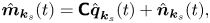 $$\begin{gather}\hat{\boldsymbol{m}}_{\boldsymbol{k}_{s}}(t) = \boldsymbol{\mathsf{C}} \hat{\boldsymbol{q}}_{\boldsymbol{k}_{s}}(t) + \hat{\boldsymbol{n}}_{\boldsymbol{k}_{s}}(t), \end{gather}$$
where  $\hat {}$ denotes the variable after Fourier transformation, the state $\hat {\boldsymbol {q}}_{\boldsymbol {k}_{s}}(t) = [\hat {u} , \hat {v} , \hat {w} , \hat {p}]^{\rm T}$ and the operators are defined as
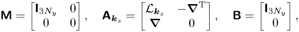 \begin{equation} \boldsymbol{\mathsf{M}} = \left[\begin{matrix} \boldsymbol{\mathsf{I}}_{3N_y} & 0 \\ 0 & 0 \end{matrix} \right], {\quad}\boldsymbol{\mathsf{A}}_{\boldsymbol{k}_{s}} = \left[\begin{matrix} \mathcal{L}_{\boldsymbol{k}_{s}} & -\boldsymbol{\nabla} ^{\rm T} \\ \boldsymbol{\nabla} & 0 \end{matrix} \right], {\quad} \boldsymbol{\mathsf{B}} = \left[ \begin{matrix} \boldsymbol{\mathsf{I}}_{3N_y} \\ 0 \end{matrix} \right], \end{equation}
where  $\boldsymbol{\mathsf{C}}$ is the spatial observation tensor, $\hat {\boldsymbol {n}}_{\boldsymbol {k}_{s}}(t)$ is the measurement noise, $\boldsymbol {\nabla }$ is the Hamiltonian operator and $\mathcal {L}_{\boldsymbol {k}_{s}}$ is the spatial linearised NS operator. The expressions of $\mathcal {L}_{\boldsymbol {k}_{s}}$, $\boldsymbol {\nabla }$ and $\boldsymbol{\mathsf{C}}$ are provided in Appendix A. Further taking Fourier transformations along the statistically homogeneous temporal direction, the linearised NS equations at each spatio-temporal scale $\boldsymbol {k} = (\boldsymbol {k}_{s},\omega )$ are obtained, as expressed by
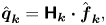 \begin{equation} \hat{\boldsymbol{q}}_{\boldsymbol{k}} = \boldsymbol{\mathsf{H}}_{\boldsymbol{k}} \boldsymbol{\cdot} \hat{\boldsymbol{f}}_{\boldsymbol{k}}, \end{equation}
where  $\boldsymbol{\mathsf{H}}_{\boldsymbol {k}}$ is the resolvent operator that is expressed as
 \begin{equation} \boldsymbol{\mathsf{H}}_{\boldsymbol{k}} = \left(-{\rm i}\omega \boldsymbol{\mathsf{M}} - \boldsymbol{\mathsf{A}}_{\boldsymbol{k}_{s}} \right)^{{-}1}, \end{equation}
with  ${\rm i}=\sqrt {-1}$. From (2.9), $\hat {\boldsymbol {q}}_{\boldsymbol {k}}$ is regarded as the response of the input forcing $\hat {\boldsymbol {f}}_{\boldsymbol {k}}$ through the resolvent operator $\boldsymbol{\mathsf{H}}_{\boldsymbol {k}}$. Taking singular value decomposition of the transfer function $\boldsymbol{\mathsf{H}}_{\boldsymbol {k}}$ yields the resolvent input and output modes ordered by the gains, where the low-order modes can be utilised to investigate the predominant coherent structures assuming the low-rank behaviour, see, e.g. Moarref et al. (Reference Moarref, Sharma, Tropp and McKeon2013) and Sharma & McKeon (Reference Sharma and McKeon2013). Meanwhile, only the linearised relationship (2.9) built by the resolvent analysis will be utilised in this study.
Based on the resolvent formulation (2.9), the RBE that estimates the flow state from limited measurements was proposed by Towne et al. (Reference Towne, Lozano-Durán and Yang2020), and is further improved (Martini et al. Reference Martini, Cavalieri, Jordan, Towne and Lesshafft2020) by considering the forcing statistics. In the following, the RBE approach is further generalised to cases where the measurements are arbitrarily sampled.
2.2. Generalised RBE in cases with arbitrary temporal measurements
In this section, the case where the information of the turbulence field is partially available from measurements that are noise contaminated and arbitrarily sampled in time is considered. Before the estimation, Fourier transformations are conducted in statistically uniform spatial directions of the flow field, such as the streamwise and spanwise directions in fully developed turbulent channel flows, leading to the decomposed measurements at separated spatial scales  $\boldsymbol {k}_{s}$. Meanwhile, since the flow signals can be unresolved in time, the Fourier transformation will not be conducted along the temporal direction. In this section, the subscript $_{\boldsymbol {k}_{s}}$ denoting the spatial scale of a flow quantity is omitted for brevity.
Consider the MIMO estimation case where the measured data are sampled at  $N_{\check {T}}$ time instances with inadequate resolution. Meanwhile, to fully resolve the temporal information, $N_T$ snapshots are actually needed $(N_T > N_{\check {T}})$. The amounts of response and observation of different types or at different locations at a given spatial scale $\boldsymbol {k}_{s}$ are denoted as $N_{q}$ and $N_{m}$, respectively. Without loss of generality, a sequence of measured data $m(j)$, where $j \in [1,N_m N_{\check {T}}]$, is taken into consideration. The linear estimation of the flow state $q(i)$, where $i \in [1,N_q N_{\check {T}}]$ is based on all the available measurements $m(j)$, can be expressed by the convolution operation as
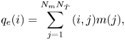 \begin{equation} q_{e}(i) =
\sum_{j=1}^{N_m N_{\check{T}}} \mathscr{h}(i,j) m(j),
\end{equation}
\begin{equation} q_{e}(i) =
\sum_{j=1}^{N_m N_{\check{T}}} \mathscr{h}(i,j) m(j),
\end{equation}
where the subscript  ${}_{e}$ denotes the estimated quantity and $\mathscr {h}(i,j)$ is the convolution kernel. Equation (2.11) can also be expressed in matrix form by
 \begin{equation} \boldsymbol{q}_{e} = \boldsymbol{\mathsf{h}} \boldsymbol{\cdot} \boldsymbol{m}, \end{equation}
where  $\boldsymbol{\mathsf{h}}$ is a two-dimensional matrix consisting of $\mathscr {h}(i,j)$ at the $(i,j)$ location.
Denoting the estimation error  $\varepsilon (i) = q(i) - q_{{e}}(i)$, the cost function $\mathcal {J}(i)$ is defined as the MSE that is expressed by
 \begin{equation} \mathcal{J}(i)=\left\langle \left| \varepsilon(i) \right|^2\right\rangle = \left\langle \left[ q(i) - \sum_{j=1}^{N_m N_{\check{T}}} \mathscr{h}(i,j) m(j) \right] {\cdot} \overline{\left[ q(i) - \sum_{k=1}^{N_m N_{\check{T}}} \mathscr{h}(i,k) m(k) \right]} \right\rangle, \end{equation}
where the overline denotes the complex conjugate and  $\langle \rangle$ denotes ensemble average. To minimise the MSE of the estimated signal with optimised transfer kernel $\mathscr {h}(i,j) = \mathscr {h}^{R}(i,j) + {\rm i} \mathscr {h}^{I}(i,j)$, the partial derivatives of the cost function $\mathcal {J}(i)$ to any $\mathscr {h}^{R}(i,j)$ or $\mathscr {h}^{I}(i,j)$ with $j \in [1,N_m N_{\check {T}}]$ should be zero, i.e.
 \begin{equation} \left.\begin{gathered} \frac{\partial \mathcal{J} (i) }{\partial \mathscr{h}^{R(I)}(i,j)} = \left\langle -2 \left[ q(i)-\sum_{j=1}^{N_m N_{\check{T}}} \mathscr{h}(i,k) m(k) \right] \overline{ m(j) } \right\rangle_{R(I)} = 0,\\ \Rightarrow \quad \left\langle q(i) \overline{m(j)} \right\rangle - \sum_{j=1}^{N_m N_{\check{T}}} \mathscr{h}(i,k) \left\langle m(k) \overline{m(j)} \right\rangle_{R(I)} = 0. \end{gathered}\right\} \end{equation}
The optimal transfer kernel can be obtained by solving the system of linear equations (2.14). The solution can be expressed as
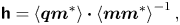 \begin{equation} \boldsymbol{\mathsf{h}} = \left\langle \boldsymbol{q} \boldsymbol{m}^{{\ast}} \right\rangle \boldsymbol{\cdot} \left\langle \boldsymbol{m} \boldsymbol{m}^{{\ast}} \right\rangle^{{-}1}, \end{equation}
where the superscript  ${}^{\ast }$ denotes the Hermitian transpose.
Equation (2.15) provides the expression of the optimal linear transfer kernel in terms of the covariance matrices of the flow state and measured signal. However, since such spatio-temporal covariance matrices are not directly available, the expressions of the optimal transfer kernel as a function of the forcing CSD tensors, which can be provided by the forcing models, should be further derived.
Considering the resolvent formulation, the expressions of  $\boldsymbol {q}$ and $\boldsymbol {m}$ in the physical space as functions of the forcing $\hat {\boldsymbol {f}}_{j}$ at $\omega _j$, where $j \in [1,N_T]$, in the Fourier space are expressed as
 $$\begin{gather} \boldsymbol{q} = \frac{1}{N_T}\sum_{j=1}^{N_T} \check{\zeta}_{\boldsymbol{q},j} \boldsymbol{\cdot} \hat{\boldsymbol{q}}_{j} = \frac{1}{N_T}\sum_{j=1}^{N_T} \check{\zeta}_{\boldsymbol{q},j} \boldsymbol{\cdot} \left( \boldsymbol{\mathsf{H}}_j \boldsymbol{\cdot} \hat{\boldsymbol{f}}_{j}\right) , \end{gather}$$
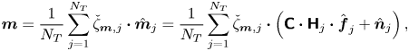 $$\begin{gather}\boldsymbol{m} = \frac{1}{N_T}\sum_{j=1}^{N_T} \check{\zeta}_{\boldsymbol{m},j} \boldsymbol{\cdot} \hat{\boldsymbol{m}}_{j} = \frac{1}{N_T} \sum_{j=1}^{N_T} \check{\zeta}_{\boldsymbol{m},j} \boldsymbol{\cdot} \left( \boldsymbol{\mathsf{C}} \boldsymbol{\cdot} \boldsymbol{\mathsf{H}}_j \boldsymbol{\cdot} \hat{\boldsymbol{f}}_{j} + \hat{\boldsymbol{n}}_{j} \right) , \end{gather}$$
where  $\hat {\boldsymbol {q}}_{j}$, $\hat {\boldsymbol {m}}_{j}$ and $\hat {\boldsymbol {n}}_{j}$ are the Fourier transforms of response, measurement and sensor noise at $\omega _j$. Here, $\check {\zeta }_{\boldsymbol {q}(\boldsymbol {m}),j} = \textrm {diag} [ \overbrace {\check {\xi }_{j}, \ldots, \check {\xi }_{j} }^{N_{q(m)}} ]$, $\check {\xi }_{j} = \textrm {e}^{\textrm {i} \omega _j \check {\boldsymbol {t}}}$, $\check {\boldsymbol {t}} \in \mathbb {R}^{N_{\check {T}}}$ is the vector consisting of the sampled time instances.
GRBE
Using (2.16a,b), the spatio-temporal covariance matrices can be predicted with the forcing models by
 $$\begin{gather} \left\langle \boldsymbol{q} \boldsymbol{m}^{{\ast}} \right\rangle_{p} = \sum_j \check{\zeta}_{\boldsymbol{q},j} \boldsymbol{\mathsf{S}}_{\boldsymbol{q}\boldsymbol{m},j} \check{\zeta}_{\boldsymbol{m},j}^{{\ast}} = \sum_j \check{\zeta}_{\boldsymbol{q},j} \boldsymbol{\mathsf{H}}_{j} \boldsymbol{\mathsf{S}}_{\boldsymbol{f}\boldsymbol{f},j} \boldsymbol{\mathsf{H}}_{\boldsymbol{m},j}^{{\ast}} \check{\zeta}_{\boldsymbol{m},j}^{{\ast}}, \end{gather}$$
 $$\begin{gather}\left\langle \boldsymbol{m} \boldsymbol{m}^{{\ast}} \right\rangle_{p} = \sum_j \check{\zeta}_{\boldsymbol{m},j} \boldsymbol{\mathsf{S}}_{\boldsymbol{m}\boldsymbol{m},j} \check{\zeta}_{\boldsymbol{m},j}^{{\ast}} = \sum_j \check{\zeta}_{\boldsymbol{m},j} \left( \boldsymbol{\mathsf{H}}_{\boldsymbol{m},j} \boldsymbol{\mathsf{S}}_{\boldsymbol{f}\boldsymbol{f},j} \boldsymbol{\mathsf{H}}_{\boldsymbol{m},j}^{{\ast}} + \boldsymbol{\mathsf{S}}_{\boldsymbol{n}\boldsymbol{n},j} \right) \check{\zeta}_{\boldsymbol{m},j}^{{\ast}}, \end{gather}$$
where  $\boldsymbol{\mathsf{S}}_{\boldsymbol {q}\boldsymbol {m},j}=\langle \hat {\boldsymbol {q}}_{j} \hat {\boldsymbol {m}}_{j}^{\ast }\rangle$, $\boldsymbol{\mathsf{S}}_{\boldsymbol {m}\boldsymbol {m},j}=\langle \hat {\boldsymbol {m}}_{j} \hat {\boldsymbol {m}}_{j}^{\ast }\rangle$, $\boldsymbol{\mathsf{S}}_{\boldsymbol {f}\boldsymbol {f},j}=\langle \hat {\boldsymbol {f}}_{j} \hat {\boldsymbol {f}}_{j}^{\ast }\rangle$ and $\boldsymbol{\mathsf{S}}_{\boldsymbol {n}\boldsymbol {n},j}=\langle \hat {\boldsymbol {n}}_{j} \hat {\boldsymbol {n}}_{j}^{\ast }\rangle$. Substituting (2.17a,b) into (2.15), the optimal transfer kernel that considers the forcing and noise statistics is expressed by
 \begin{align} \boldsymbol{\mathsf{h}}&=\left\langle \boldsymbol{q} \boldsymbol{m}^{{\ast}} \right\rangle_{p} \boldsymbol{\cdot} \left\langle \boldsymbol{m} \boldsymbol{m}^{{\ast}} \right\rangle_{p}^{{-}1} \end{align}
 \begin{align} &=\left( \sum_j \check{\zeta}_{\boldsymbol{q},j} \boldsymbol{\mathsf{S}}_{\boldsymbol{q}\boldsymbol{m},j} \check{\zeta}_{\boldsymbol{m},j}^{{\ast}} \right) \boldsymbol{\cdot} \left( \sum_j \check{\zeta}_{\boldsymbol{m},j} \boldsymbol{\mathsf{S}}_{\boldsymbol{m}\boldsymbol{m},j} \check{\zeta}_{\boldsymbol{m},j}^{{\ast}}\right) ^{{-}1} \end{align}
 \begin{align} &=\left[ \sum_j \check{\zeta}_{\boldsymbol{q},j} \boldsymbol{\mathsf{H}}_{j} \boldsymbol{\mathsf{S}}_{\boldsymbol{f}\boldsymbol{f},j} \boldsymbol{\mathsf{H}}_{\boldsymbol{m},j}^{{\ast}} \check{\zeta}_{\boldsymbol{m},j}^{{\ast}} \right] \boldsymbol{\cdot} \left[ \sum_j \check{\zeta}_{\boldsymbol{m},j} \left( \boldsymbol{\mathsf{H}}_{\boldsymbol{m},j} \boldsymbol{\mathsf{S}}_{\boldsymbol{f}\boldsymbol{f},j} \boldsymbol{\mathsf{H}}_{\boldsymbol{m},j}^{{\ast}} + \boldsymbol{\mathsf{S}}_{\boldsymbol{n}\boldsymbol{n},j} \right) \check{\zeta}_{\boldsymbol{m},j}^{{\ast}}\right] ^{{-}1}. \end{align}
 From the above derivations, the transfer kernel  $\boldsymbol{\mathsf{h}}$ is the optimal linear estimator of the response $\boldsymbol {q}$ when the real statistics $\boldsymbol{\mathsf{S}}_{\boldsymbol {ff},j}$ and $\boldsymbol{\mathsf{S}}_{\boldsymbol {nn},j}$ are incorporated, which can be obtained from another existing database. More importantly, the transfer kernel defined in (2.18) also constructs an open framework that enables the incorporation of the spatio-temporal forcing models that predict the forcing CSD tensors all over the frequency domain at each spatial scale $\boldsymbol {k}_{s}$ when the real statistics of forcing are unknown. The current models that provide spatio-temporal prediction of the forcing include the baseline model (B-model) (Hwang & Cossu Reference Hwang and Cossu2010; Madhusudanan et al. Reference Madhusudanan, Illingworth and Marusic2019), W-model and
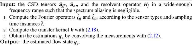
  $\lambda$-model (Gupta et al. Reference Gupta, Madhusudanan, Wan, Illingworth and Juniper2021), which assume that the forcing is white in time and uncorrelated in space with certain forms of spatial energy distributions along the wall-normal height. These forcing models are reviewed in Appendix B. The new approach generalises the RBE to the cases with arbitrary sampled measurements in time, and thus it is denoted as the GRBE in this study. The procedure of the GRBE is provided in Algorithm 1.
2.3. Expected estimation error from the GRBE
In § 2.2, the theoretically optimal transfer kernel of arbitrarily sampled measurements is derived in (2.18). On the other hand, the expected statistics of the estimation error can also be theoretically derived. Recall (2.13) that describes the linear relationship between the observations and estimations, the matrix form holds
 \begin{align} \left\langle \boldsymbol{\varepsilon} \boldsymbol{\varepsilon}^{{\ast}} \right\rangle & = \left\langle \left( \boldsymbol{q} - \boldsymbol{\mathsf{h}} \boldsymbol{\cdot} \boldsymbol{m} \right) \boldsymbol{\cdot} \left( \boldsymbol{q} - \boldsymbol{\mathsf{h}} \boldsymbol{\cdot} \boldsymbol{m} \right)^{{\ast}} \right\rangle \nonumber\\ & = \left\langle \boldsymbol{q} \boldsymbol{q}^{{\ast}} \right\rangle + \boldsymbol{\mathsf{h}} \boldsymbol{\cdot} \left\langle \boldsymbol{m} \boldsymbol{m}^{{\ast}} \right\rangle \boldsymbol{\cdot} \boldsymbol{\mathsf{h}}^{{\ast}} - \left\langle \boldsymbol{q} \boldsymbol{m}^{{\ast}} \right\rangle \boldsymbol{\cdot} \boldsymbol{\mathsf{h}}^{{\ast}} - \boldsymbol{\mathsf{h}} \boldsymbol{\cdot} \left\langle \boldsymbol{m} \boldsymbol{q}^{{\ast}} \right\rangle . \end{align}
 When the actual forcing and noise statistics are incorporated into the transfer kernel  $\boldsymbol{\mathsf{h}}$, the minimum expected estimation error can be obtained, as calculated by
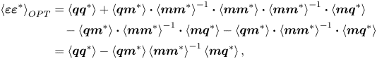 \begin{align} \left\langle \boldsymbol{\varepsilon} \boldsymbol{\varepsilon}^{{\ast}} \right\rangle_{OPT} & = \left\langle \boldsymbol{q} \boldsymbol{q}^{{\ast}} \right\rangle + \left\langle {\boldsymbol{q}} {\boldsymbol{m}}^{ {\ast}} \right\rangle \boldsymbol{\cdot} \left\langle {\boldsymbol{m}} {\boldsymbol{m}}^{{\ast}} \right\rangle^{{-}1} \boldsymbol{\cdot} \left\langle \boldsymbol{m} \boldsymbol{m}^{{\ast}} \right\rangle \boldsymbol{\cdot} \left\langle {\boldsymbol{m}} {\boldsymbol{m}}^{{\ast}} \right\rangle^{{-}1} \boldsymbol{\cdot} \left\langle {\boldsymbol{m}} {\boldsymbol{q}}^{ {\ast}} \right\rangle\nonumber\\ &\quad- \left\langle \boldsymbol{q} \boldsymbol{m}^{{\ast}} \right\rangle \boldsymbol{\cdot} \left\langle {\boldsymbol{m}} {\boldsymbol{m}}^{{\ast}} \right\rangle^{{-}1} \boldsymbol{\cdot} \left\langle {\boldsymbol{m}} {\boldsymbol{q}}^{ {\ast}} \right\rangle - \left\langle {\boldsymbol{q}} {\boldsymbol{m}}^{ {\ast}} \right\rangle \boldsymbol{\cdot} \left\langle {\boldsymbol{m}} {\boldsymbol{m}}^{{\ast}} \right\rangle^{{-}1} \boldsymbol{\cdot} \left\langle \boldsymbol{m} \boldsymbol{q}^{{\ast}} \right\rangle \nonumber\\ & = \left\langle \boldsymbol{q} \boldsymbol{q}^{{\ast}} \right\rangle - \left\langle \boldsymbol{q} \boldsymbol{m}^{{\ast}} \right\rangle \left\langle \boldsymbol{m} \boldsymbol{m}^{{\ast}} \right\rangle^{{-}1} \left\langle \boldsymbol{m} \boldsymbol{q}^{{\ast}} \right\rangle, \end{align}
where the subscript ‘ $_{OPT}$’ denotes the variable from the optimal linear estimation. Considering that $\langle \boldsymbol {q} \boldsymbol {m}^{\ast } \rangle \langle \boldsymbol {m} \boldsymbol {m}^{\ast } \rangle ^{-1} \langle \boldsymbol {m} \boldsymbol {q}^{\ast } \rangle = \langle \boldsymbol {q}_{e} \boldsymbol {q}_{e}^{\ast } \rangle$ according to (2.12) and (2.18a), (2.20) indicates the orthogonality principle for the optimal linear estimation, i.e. $\langle \boldsymbol {q}_{e} \boldsymbol {\cdot } \boldsymbol {\varepsilon }^{\ast } \rangle = \boldsymbol{\mathsf{O}}$. Considering (2.16), the covariance matrix of the estimated error is further expressed by
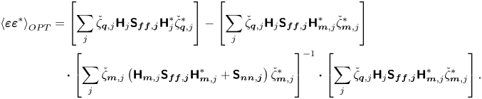 \begin{align} \left\langle \boldsymbol{\varepsilon} \boldsymbol{\varepsilon}^{{\ast}} \right\rangle_{OPT} &= \left[ \sum_j \check{\zeta}_{\boldsymbol{q},j} \boldsymbol{\mathsf{H}}_{j} \boldsymbol{\mathsf{S}}_{\boldsymbol{f}\boldsymbol{f},\boldsymbol{j}} \boldsymbol{\mathsf{H}}_{j}^{{\ast}} \check{\zeta}_{\boldsymbol{q},j}^{{\ast}} \right] - \left[ \sum_j \check{\zeta}_{\boldsymbol{q},j} \boldsymbol{\mathsf{H}}_{j} \boldsymbol{\mathsf{S}}_{\boldsymbol{f}\boldsymbol{f},\boldsymbol{j}} \boldsymbol{\mathsf{H}}_{\boldsymbol{m},j}^{{\ast}} \check{\zeta}_{\boldsymbol{m},j}^{{\ast}} \right]\nonumber\\ &\quad \boldsymbol{\cdot} \left[\sum_j \check{\zeta}_{\boldsymbol{m},j} \left( \boldsymbol{\mathsf{H}}_{\boldsymbol{m},j} \boldsymbol{\mathsf{S}}_{\boldsymbol{f}\boldsymbol{f},\boldsymbol{j}} \boldsymbol{\mathsf{H}}_{\boldsymbol{m},j}^{{\ast}} + \boldsymbol{\mathsf{S}}_{\boldsymbol{n}\boldsymbol{n},\boldsymbol{j}} \right) \check{\zeta}_{\boldsymbol{m},j}^{{\ast}} \right]^{{-}1} \boldsymbol{\cdot} \left[ \sum_j \check{\zeta}_{\boldsymbol{q},j} \boldsymbol{\mathsf{H}}_{j} \boldsymbol{\mathsf{S}}_{\boldsymbol{f}\boldsymbol{f},\boldsymbol{j}} \boldsymbol{\mathsf{H}}_{\boldsymbol{m},j}^{{\ast}} \check{\zeta}_{\boldsymbol{m},j}^{{\ast}} \right]. \end{align}
On the other hand, when the forcing models rather than the real flow statistics are incorporated in the GRBE estimator, the orthogonal principle as in (2.20) for the optimal linear estimation no longer holds. Instead, the expected error energy from the modelled GRBE estimator should be directly derived from (2.19) by considering (2.18a), i.e.
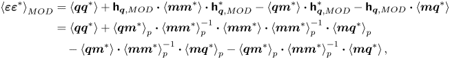 \begin{align} \left\langle {\boldsymbol{\varepsilon}} {\boldsymbol{\varepsilon}}^{{\ast}} \right\rangle_{MOD} & = \left\langle \boldsymbol{q} \boldsymbol{q}^{{\ast}} \right\rangle + \boldsymbol{\mathsf{h}}_{\boldsymbol{q},{MOD}} \boldsymbol{\cdot} \left\langle \boldsymbol{m} \boldsymbol{m}^{{\ast}} \right\rangle \boldsymbol{\cdot} \boldsymbol{\mathsf{h}}_{\boldsymbol{q},{MOD}}^{{\ast}} - \left\langle \boldsymbol{q} \boldsymbol{m}^{{\ast}} \right\rangle \boldsymbol{\cdot} \boldsymbol{\mathsf{h}}_{\boldsymbol{q},{MOD}}^{{\ast}} - \boldsymbol{\mathsf{h}}_{\boldsymbol{q},{ MOD}} \boldsymbol{\cdot} \left\langle \boldsymbol{m} \boldsymbol{q}^{{\ast}} \right\rangle\nonumber\\ & = \left\langle \boldsymbol{q} \boldsymbol{q}^{{\ast}} \right\rangle + \left\langle {\boldsymbol{q}} {\boldsymbol{m}}^{ {\ast}} \right\rangle_{p} \boldsymbol{\cdot}\left\langle {\boldsymbol{m}} {\boldsymbol{m}}^{{\ast}} \right\rangle_{p}^{{-}1} \boldsymbol{\cdot} \left\langle \boldsymbol{m} \boldsymbol{m}^{{\ast}} \right\rangle \boldsymbol{\cdot} \left\langle {\boldsymbol{m}} {\boldsymbol{m}}^{{\ast}} \right\rangle_{p}^{{-}1} \boldsymbol{\cdot} \left\langle {\boldsymbol{m}} {\boldsymbol{q}}^{ {\ast}} \right\rangle_{p}\nonumber\\ &\quad - \left\langle \boldsymbol{q} \boldsymbol{m}^{{\ast}} \right\rangle \boldsymbol{\cdot} \left\langle {\boldsymbol{m}} {\boldsymbol{m}}^{{\ast}} \right\rangle_{p}^{{-}1} \boldsymbol{\cdot} \left\langle {\boldsymbol{m}} {\boldsymbol{q}}^{ {\ast}} \right\rangle_{p} - \left\langle {\boldsymbol{q}} {\boldsymbol{m}}^{ {\ast}} \right\rangle_{p} \boldsymbol{\cdot} \left\langle {\boldsymbol{m}} {\boldsymbol{m}}^{{\ast}} \right\rangle_{p}^{{-}1} \boldsymbol{\cdot} \left\langle \boldsymbol{m} \boldsymbol{q}^{{\ast}} \right\rangle, \end{align}
where  $\langle {\boldsymbol {q}} {\boldsymbol {m}}^{ \ast } \rangle _{p}$ and $\langle {\boldsymbol {m}} {\boldsymbol {m}}^{ \ast } \rangle _{p}$ are defined in (2.17) and the subscript ‘ $_{MOD}$’ denotes the variable corresponding to the linear estimation informed by the modelled forcing. Substituting the estimation error from optimal linear estimation in (2.20) to (2.22), the estimation error from the modelled forcing can be expressed as
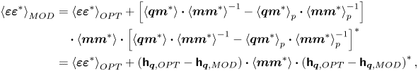 \begin{align} \left\langle {\boldsymbol{\varepsilon}} {\boldsymbol{\varepsilon}}^{{\ast}} \right\rangle_{MOD} & = \left\langle {\boldsymbol{\varepsilon}} {\boldsymbol{\varepsilon}}^{{\ast}} \right\rangle_{OPT} + \left[ \left\langle {\boldsymbol{q}} {\boldsymbol{m}}^{ {\ast}} \right\rangle \boldsymbol{\cdot} \left\langle {\boldsymbol{m}} {\boldsymbol{m}}^{{\ast}} \right\rangle^{{-}1} - \left\langle {\boldsymbol{q}} {\boldsymbol{m}}^{ {\ast}} \right\rangle_{p} \boldsymbol{\cdot} \left\langle {\boldsymbol{m}} {\boldsymbol{m}}^{{\ast}} \right\rangle_{p}^{{-}1} \right] \nonumber\\ &\quad \boldsymbol{\cdot} \left\langle {\boldsymbol{m}} {\boldsymbol{m}}^{{\ast}} \right\rangle \boldsymbol{\cdot} \left[ \left\langle {\boldsymbol{q}} {\boldsymbol{m}}^{ {\ast}} \right\rangle \boldsymbol{\cdot} \left\langle {\boldsymbol{m}} {\boldsymbol{m}}^{{\ast}} \right\rangle^{{-}1} - \left\langle {\boldsymbol{q}} {\boldsymbol{m}}^{ {\ast}} \right\rangle_{p} \boldsymbol{\cdot} \left\langle {\boldsymbol{m}} {\boldsymbol{m}}^{{\ast}} \right\rangle_{p}^{{-}1} \right]^{{\ast}}\nonumber\\ & = \left\langle {\boldsymbol{\varepsilon}} {\boldsymbol{\varepsilon}}^{{\ast}} \right\rangle_{OPT} + \left( \boldsymbol{\mathsf{h}}_{\boldsymbol{q},{OPT}} - \boldsymbol{\mathsf{h}}_{\boldsymbol{q},{MOD}} \right) \boldsymbol{\cdot} \left\langle {\boldsymbol{m}} {\boldsymbol{m}}^{{\ast}} \right\rangle \boldsymbol{\cdot} \left( \boldsymbol{\mathsf{h}}_{\boldsymbol{q},{OPT}} - \boldsymbol{\mathsf{h}}_{\boldsymbol{q},{MOD}} \right)^{{\ast}}, \end{align}
where  $\boldsymbol{\mathsf{h}}_{\boldsymbol {q},{OPT}}=\langle {\boldsymbol {q}} {\boldsymbol {m}}^{ \ast } \rangle \boldsymbol {\cdot } \langle {\boldsymbol {m}} {\boldsymbol {m}}^{\ast } \rangle ^{-1}$. On the right-hand side of (2.23), the extra term $[ ( \boldsymbol{\mathsf{h}}_{\boldsymbol {q},{OPT}} - \boldsymbol{\mathsf{h}}_{\boldsymbol {q},{MOD}} ) \boldsymbol {\cdot } \langle {\boldsymbol {m}} {\boldsymbol {m}}^{\ast } \rangle \boldsymbol {\cdot } ( \boldsymbol{\mathsf{h}}_{\boldsymbol {q},{OPT}} - \boldsymbol{\mathsf{h}}_{\boldsymbol {q},{MOD}} )^{\ast } ]$ is positive semi-definite. Thus, the estimation error energy from the modelled forcing will be minimised when $\boldsymbol{\mathsf{h}}_{\boldsymbol {q},{MOD}} = \boldsymbol{\mathsf{h}}_{\boldsymbol {q},{OPT}}$.
2.4. Discussions on the relationship between the GRBE and RBE
The GRBE fundamentally differs from the RBE (Martini et al. Reference Martini, Cavalieri, Jordan, Towne and Lesshafft2020) in their different optimisation targets when constructing the transfer kernel. The RBE minimises the expected error energy at each frequency, while the GRBE directly minimises the expected error energy in physical space. Although these two approaches provide the same results when the measurements are temporally resolved, their results are different when the measurement information is unresolved in time. We will elaborate the discussions between the GRBE and RBE in the following.
2.4.1. Temporally resolved measurements
The RBE transfer function that minimises the expected error energy at a given frequency is given by (Martini et al. Reference Martini, Cavalieri, Jordan, Towne and Lesshafft2020)
 \begin{equation} \hat{\boldsymbol{T}} = \boldsymbol{H} \boldsymbol{S}_{\boldsymbol{f}\boldsymbol{f}} {\boldsymbol{H}_{\boldsymbol{m}}^{{\ast}}} \left( {\boldsymbol{H}_{\boldsymbol{m}}} \boldsymbol{S}_{\boldsymbol{f}\boldsymbol{f}} {\boldsymbol{H}_{\boldsymbol{m}}^{{\ast}}} + \boldsymbol{S}_{\boldsymbol{n}\boldsymbol{n}} \right)^{{-}1}. \end{equation}
The estimated  $\hat {\boldsymbol {q}}_{e}$ is obtained with
 \begin{equation} \hat{\boldsymbol{q}}_{{e},j} =\hat{\boldsymbol{T}}_{j} \boldsymbol{\cdot} \hat{\boldsymbol{m}}_j. \end{equation}
When the measurements are temporally resolved, the RBE approach can be applied in the time domain through inverse Fourier transform (Martini et al. Reference Martini, Cavalieri, Jordan, Towne and Lesshafft2020; Amaral et al. Reference Amaral, Cavalieri, Martini, Jordan and Towne2021) i.e.
 \begin{equation} \boldsymbol{h}^{RBE} \left( t,\tau \right) =\mathcal{F}^{{-}1}\left( \hat{\boldsymbol{T}} (\omega) \right) =\frac{1}{2 {\rm \pi}}\int_{-\infty}^{\infty} \hat{\boldsymbol{T}}(\omega)\exp({{\rm i} \omega ( t-\tau ) })\,{\rm d}\omega, \end{equation}
and the flow state  $\boldsymbol {q}$ can be estimated by performing a convolution of the transfer kernel $\boldsymbol {h}^{RBE}$ and the measurements $\boldsymbol {m}$,
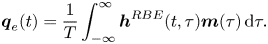 \begin{equation} \boldsymbol{q}_{e}(t) = \frac{1}{T} \int_{-\infty}^{\infty}\boldsymbol{h}^{RBE}(t,\tau ) \boldsymbol{m}( \tau )\,{\rm d}\tau. \end{equation}
Given temporally resolved information, the discrete form of the convolution operation of the RBE is expressed by
 \begin{equation} \boldsymbol{q}_{e} = \boldsymbol{\mathsf{h}}^{RBE} \boldsymbol{\cdot} \boldsymbol{m}, \end{equation}
with
 \begin{align} \boldsymbol{\mathsf{h}}^{RBE}&=\sum_{j} \zeta_{\boldsymbol{q},j} \hat{\boldsymbol{\mathsf{T}}}(\omega_j) \zeta_{\boldsymbol{m},j}^{{\ast}} \nonumber\\ &=\sum_{j} \zeta_{\boldsymbol{q},j}\boldsymbol{H} \boldsymbol{S}_{\boldsymbol{f}\boldsymbol{f}} {\boldsymbol{H}_{\boldsymbol{m}}^{{\ast}}} \left( {\boldsymbol{H}_{\boldsymbol{m}}} \boldsymbol{S}_{\boldsymbol{f}\boldsymbol{f}} {\boldsymbol{H}_{\boldsymbol{m}}^{{\ast}}} + \boldsymbol{S}_{\boldsymbol{n}\boldsymbol{n}} \right)^{{-}1} \zeta_{\boldsymbol{m},j}^{{\ast}}, \end{align}
where  ${\zeta }_{\boldsymbol {q}(\boldsymbol {m}),j} = \textrm {diag} [ \overbrace {{\xi }_{j}, \ldots, {\xi }_{j} }^{N_{q(m)}} ]$, ${\xi }_{j} = \textrm {e}^{\textrm {i} \omega _j \boldsymbol {t}}$, $\boldsymbol {t} \in \mathbb {R}^{N_{{T}}}$ is the vector consisting of fine enough time steps that are evenly distributed. Comparing the RBE transfer kernel (2.29) with the GRBE one (2.18c), it can be demonstrated that these two transfer kernels are the same only when $\check {\zeta }_{\boldsymbol {q}(\boldsymbol {m}),j}=\zeta _{\boldsymbol {q}(\boldsymbol {m}),j}$.
It should be noted that the above relationship between the GRBE and RBE is only valid when the measurement information is resolved in time. In the other cases, these two approaches are different due to their essential difference in constructing the transfer kernel. In the next subsection, the implementations of the RBE in temporally unresolved cases will be provided to facilitate further comparisons between the GRBE and RBE.
RBE-F

2.4.2. Implementations of the RBE in temporally unresolved cases
When the sampling time steps are not fine enough to resolve the flow data, the convolution operation (2.27) of RBE cannot be well approximated by the discrete counterpart (2.28) with the temporally unresolved measurements, even if the spatio-temporal statistics of the flow state are available. Despite this, if the RBE is to be deployed in such case, there are two different choices of directly applying the RBE formulation in the frequency or temporal domain, i.e.
(i) To conduct the discrete Fourier transformation (DFT) of the measurements with the sparse-in-time signal, then estimate the flow state via (2.25) in the frequency domain. Since this approach estimates the flow state with a discrete-in-frequency resolvent-based transfer function, it is denoted as RBE-F in the following section. The procedure of RBE-F is provided in Algorithm 2.
(ii) To deploy the discrete RBE convolution formulation (2.28) in estimating the sparse-in-time flow state. To discretise the RBE transfer kernel in sparse time instances, it is calculated by
 \begin{equation} \boldsymbol{\mathsf{h}}^{RBE}(i,j) =\int_{\Delta t_{j-}}^{\Delta t_{j+}} w(\tau) \boldsymbol{h}^{RBE}(t_i,t_j + \tau)\, {\rm d}\tau, \end{equation}
 where  $\Delta t_{j-} = (t_{j-1}-t_{j})/2$, $\Delta t_{j+} = (t_{j+1}-t_{j})/2$ and $w(\tau )$ is the weighting function for integration, which is specified as $w(\tau )=1$ in this study. Since this approach utilises a discrete-in-time resolvent-based transfer kernel, it is denoted as RBE-T in the following section. The procedure of the RBE-T is provided in Algorithm 3.
From the above discussions, both RBE-F and RBE-T, although seemingly straightforward, utilise different assumptions when applied in temporally unresolved cases. Investigations on the sources of estimation errors of such two variants of the RBE are provided in Appendix C. For the validations of the GRBE in § 3, only the RBE-T approach will be included, since RBE-T can be directly applied in the cases with uneven samplings in time.
Besides the non-causal estimation applied in post-processing of the measured data, the causal estimation that utilises only the measurements up to the current time step in real-time estimation is also an interesting topic. Since the GRBE does not impose any restrictions on the temporal resolution of the measurements, it is naturally capable of providing an optimal causal estimation of the flow state in real-time estimation when informed by the actual forcing colour. On the other hand, as described in Martini et al. (Reference Martini, Cavalieri, Jordan, Towne and Lesshafft2020), the RBE can also be applied for causal estimation by truncating the resolvent-based kernel (2.26) by setting  $\boldsymbol{\mathsf{h}}^{RBE} ( t,\tau )=0$ when $\tau > t$, which is essentially different from the causal GRBE approach. The discussions on the RBE and GRBE results in causal estimation are provided in § 3.1.2.
RBE-T
3. Validations
To validate the new estimation framework, two cases, i.e. the complex Ginzburg–Landau equation and turbulent channel flows with friction Reynolds numbers  $Re_{\tau } = 186$, 547 and 934, will be used in this section. The RBE (Martini et al. Reference Martini, Cavalieri, Jordan, Towne and Lesshafft2020; Towne et al. Reference Towne, Lozano-Durán and Yang2020) and the $H_2$-optimal estimation (Illingworth et al. Reference Illingworth, Monty and Marusic2018) are also included in this section for comparison. To extend the RBE in temporally unresolved cases, the RBE-T defined in § 2.4.2 is utilised. For brevity, we will still use the term ‘RBE’ to refer to the RBE-T approach in this section unless otherwise specified. For reference, the details of the $H_2$-optimal estimation method are provided in Appendix D. In all the cases tested in this section, the measurement noise is neglected for brevity.
3.1. The complex Ginzburg–Landau equation
The complex Ginzburg–Landau equation is a one-dimensional model that mimics a real turbulence system (Bagheri, Brandt & Henningson Reference Bagheri, Brandt and Henningson2009; Towne, Schmidt & Colonius Reference Towne, Schmidt and Colonius2018; Towne et al. Reference Towne, Lozano-Durán and Yang2020) and facilitates the analysis of the properties of the linear operator. The equation can be written in the same form as (2.7a), with the linear operators  $\boldsymbol{\mathsf{A}}$, $\boldsymbol{\mathsf{B}}$ and $\boldsymbol{\mathsf{M}}$ expressed by
 \begin{equation} \left.\begin{gathered} \boldsymbol{\mathsf{A}} ={-} \nu \frac{\partial}{\partial x} + \gamma \frac{{\partial}^2}{\partial x^2} + \mu (x), \\ \boldsymbol{\mathsf{M}} = \boldsymbol{\mathsf{B}} = \boldsymbol{\mathsf{I}}. \end{gathered}\right\} \end{equation}
The parameters in (3.1) are set as  $\mu (x) = (\mu _0 - c_u^2) + \mu _2 x^2 / 2$, $\nu = 2+0.2\textrm {i}$, $\gamma = 1-\textrm {i}$, $\nu _0 = 0.3$, $c_u = 0.2$ and $\mu _2 = -0.01$, which are identical to those in Towne et al. (Reference Towne, Schmidt and Colonius2018). The spatial domain is discretised with second-order upwind scheme at evenly distributed grid nodes with $N_x = 221$ in a computational domain $x \in [ -85,85 ]$, where the grid size $\Delta x = 0.77$. Following Towne et al. (Reference Towne, Schmidt and Colonius2018), the input forcing that excites the system is realised by setting the value at each discrete time step (with a constant step size of 0.05) and grid node to be a random complex number with uniformly distributed phase from 0 to $2 {\rm \pi}$ and normally distributed amplitude with unit variance. The forcing is then low-pass filtered using a tenth-order finite-impulse-response filter with a cutoff frequency equal to $60\,\%$ of the Nyquist frequency $\omega _{s}$ equal to $20 {\rm \pi}$. The spatial scope of forcing is limited in the interior of the computational domain with an exponential envelope of $\textrm {exp} [ -( x/L )^p ]$, where $L = 60$ and $p = 10$. The equations are integrated in time with the Crank–Nicolson scheme (Crank & Nicolson Reference Crank and Nicolson1947). After the computational result achieves a statistical stationary state, the flow data at the measurement location are sampled for estimation.
3.1.1. Non-causal estimation results
In this section, three cases in terms of different sampling time intervals are considered in this section, namely the temporally resolved case (TR), the randomly sampled case (RS) and the temporally unresolved case (TU), with  $\Delta t = 0.5$, $\Delta t = \textrm {rand}(0.5,8.0)$ that is uniformly distributed between 0.5 and 8.0, and $\Delta t = 8.0$, respectively. The same sampling period of $T = 200$ is applied for each case. To construct the estimator of the GRBE in (2.18) and RBE in (2.24), the incorporated CSD tensor of the forcing is set to be $\boldsymbol{\mathsf{S}}_{\boldsymbol {ff}} = \boldsymbol{\mathsf{I}}$ at each frequency.
In the TR case with  $\Delta t = 0.5$, the temporal information of the measured signals is resolved in time. In this case, the flow information at the energy-containing temporal scales can be well recovered by the Fourier transform. According to the derivations in § 2.4, the RBE results should be the same as the GRBE in this case. Figure 1(a,d) depicts the estimation of the flow data at $x = 10$ using the measurements at $x = 0$. It is observed that the prediction results of the RBE are the same as those of the GRBE, which match pretty well with the reference numerical results. To quantitatively analyse the dependence of estimation accuracy on the distance between the measured and predicted signals, the relative MSE at the $i$th location is defined as
 \begin{equation} {\rm Err} = \frac{\left\langle\sum_{j=1}^{N_{\check{T}}} \left| \varepsilon(i,j) \right| ^2 \right\rangle}{\left\langle \sum_{j=1}^{N_{\check{T}}} \left| u(i,j) \right| ^2 \right\rangle}, \end{equation}
where  $\varepsilon (i,j) = u(i,j)-u_{e}(i,j)$ is the error at the $i$th location and $j$th time instance. Figure 2(a) shows the relative MSEs of the estimations at different spatial locations in the TR case. The relative MSEs from the RBE and GRBE overlap with each other at all of the considered locations.
Estimation of the flow states at  $x = 10$ using the measurements at $x = 0$ with the GRBE (a–c) and RBE (d–f) in cases TR (a,d), RS (b,e) and TU (c,f). The solid and dashed curves denote the reference numerical results and the estimated ones, respectively.
Relative MSEs of the estimations with measurements at  $x=0$ in cases TR ( $a$), RS ( $b$) and TU ( $c$). The translucent grey curves denote the spatial distribution of the relative fluctuation energy from the reference numerical simulation.
In the RS case, the sampling time steps are set to be uniformly distributed in the range of  $0.5 \leqslant t \leqslant 8.0$. From figure 1(b,e), the GRBE results match well with the reference numerical results, while those from the RBE deviate obviously from the reference data. In figure 2(b), the relative MSEs of the RBE increase rapidly when moving away from the measurement location, while those of the GRBE are much lower at corresponding locations. Similar phenomena are observed in the TU case, where the estimation accuracy of the GRBE is also much lower than the RBE.
3.1.2. Causal estimation results
In Martini et al. (Reference Martini, Cavalieri, Jordan, Towne and Lesshafft2020), the casual RBE estimator is proposed by truncating the resolvent-based kernel (2.26), which can be explicitly expressed in (2.30) with the weighting function  $w(\tau )=0$ when $\tau > t$, where $t$ is the estimation time step. On the other hand, the causal GRBE estimator can be realised by setting $\check {\boldsymbol {t}}$ containing only the time instances with $\tau = t$ and $\tau \leqslant t$ when constructing the Fourier bases $\check {\zeta }_{\boldsymbol {q},j}$ and $\check {\zeta }_{\boldsymbol {m},j}$ in (2.18), respectively.
Figures 3 and 4 show the estimated instantaneous flow states and relative MSEs of the one-dimensional Ginzburg–Landau equation with measurements located at  $x=0$. The sampling time interval is set as $\Delta t = 0.5$, which is the same as that in the TR case. Since the $H_2$-optimal estimation provides optimal causal results with white-in-time forcing (Doyle et al. Reference Doyle, Glover, Khargonekar and Francis1989; Zhou & Doyle Reference Zhou and Doyle1998), which is met in this case, its results are used for the validation of the causal GRBE herein. From figures 3 and 4, the causal GRBE results overlap with the $H_2$-optimal estimation results at all of the tested locations. On the other hand, the estimation errors from the causal RBE results are obviously larger than those from the causal GRBE results at $x < 0$. Even in the downstream region with $x \geqslant 0$, the estimation errors of the causal RBE estimator are still subtly larger than those of the causal GRBE estimator, as in figure 4(b). Such observations are consistent with those in Martini et al. (Reference Martini, Cavalieri, Jordan, Towne and Lesshafft2020), where the causal RBE results are found to underestimate the flow state compared with the causal Kalman filter results.
Causal estimation of the flow states at  $x = -1.5$ (a,c,e) and $x=10$ (b,d,f) using the measurements at $x = 0$ with the $H_2$-optimal estimation (a,b), GRBE (c,d) and RBE (e,f). The solid and dashed curves denote the reference numerical results and the estimated ones, respectively.
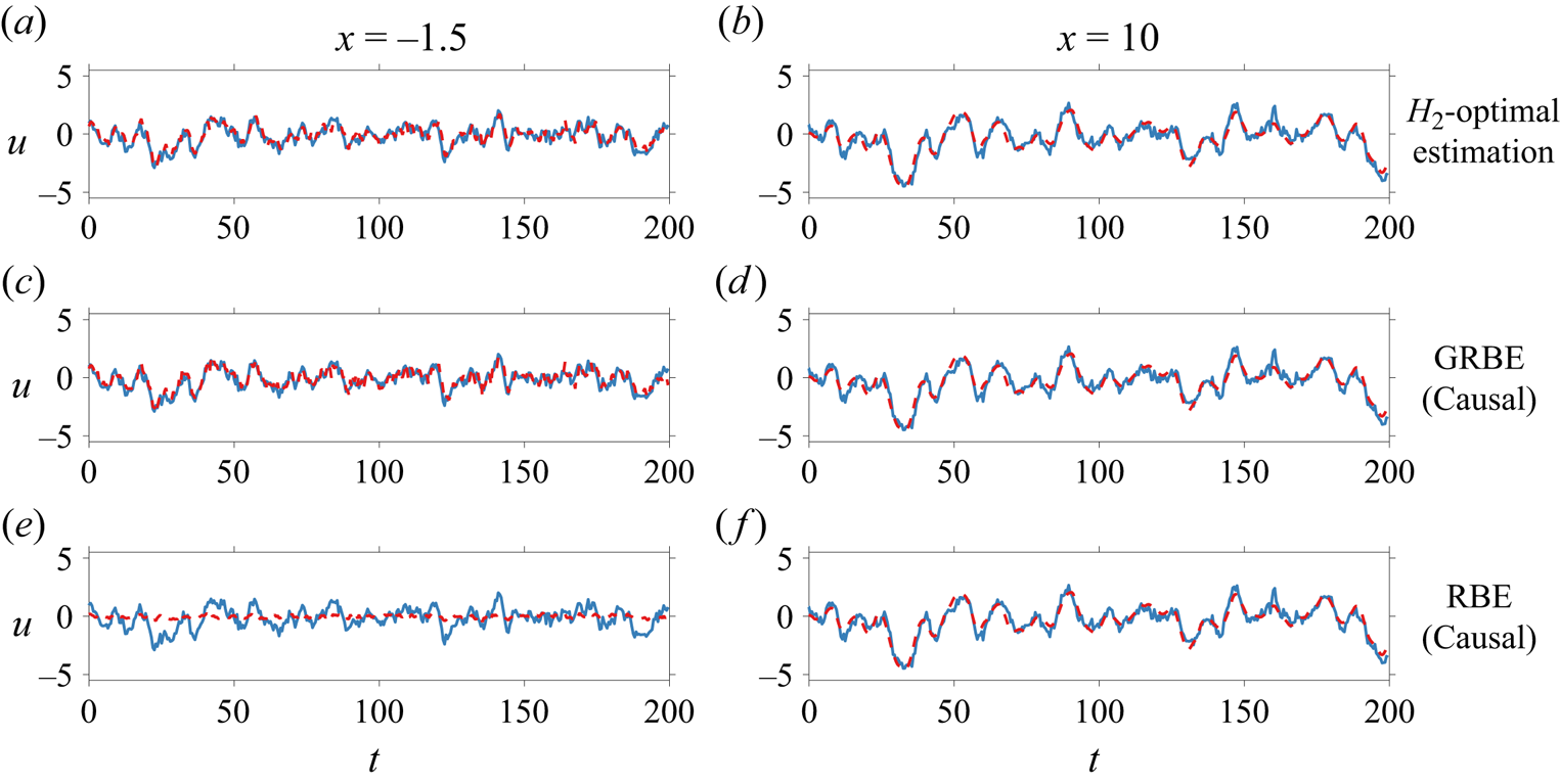
Relative MSEs of the causal estimations with measurements at  $x=0$ ( $a$), with zoomed results near $x=0$ ( $b$). The translucent grey curves denote the spatial distribution of the relative fluctuation energy from the reference numerical simulation.
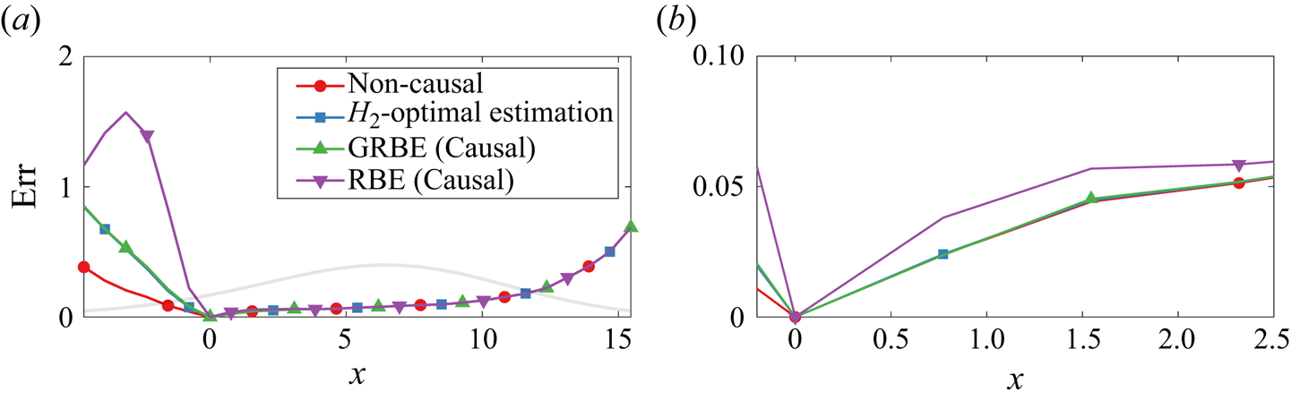
3.2. Estimation of the turbulent channel flows
In this section, validations of the GRBE in estimating the turbulent channel flows with  $Re_{\tau } = 186$, 547 and 934 will be conducted, where the RBE results are also presented.
3.2.1. Descriptions of the DNS database
The code that is used to generate the widely used open-source DNS database (Del Alamo & Jiménez Reference Del Alamo and Jiménez2003; Hoyas & Jiménez Reference Hoyas and Jiménez2008) for incompressible turbulent channel flows with  $Re_{\tau}=186$, 547 and 934 is applied to compute the DNS results in this study. Details of the DNS set-ups are listed in table 1. To provide temporally resolved results, the sampling time intervals $\delta t^+=\delta t {\cdot } u_{\tau }^2 / \nu$ are set as 2.13, 4.81 and 5.09 for cases with $Re_{\tau } = 186$, 547 and 934, respectively. The normalised total simulation time $(u_\tau {\cdot } T)/h$ is larger than 5.0 in each case to obtain statistically converged results. To process the DNS datasets, the computational domain is divided into blocks with a spatial size of ${L_x}/h = 4{\rm \pi}$, ${L_z}/h = {\rm \pi}$ and ${L_y}/h = 2$ in each case. Considering that the fully developed channel flow is statistically symmetric about the centreline $y=h$, the DNS data that are mirrored about the centreline are treated as another set of blocks besides the original one. The time periods of the blocks are set as $240\delta t$, $160\delta t$ and $160\delta t$ for cases with $Re_{\tau } = 186$, 547 and 934, respectively, with $75\,\%$ overlap in the temporal direction. The rectangular window function is utilised for spectral analysis. With the above set-ups for data processing, the numbers of blocks are 408, 352 and 252 for cases with $Re_{\tau } = 186$, 547 and 934, respectively. The DNS datasets utilised in this study have been validated in Ying et al. (Reference Ying, Liang, Li and Fu2023) by comparisons with the time-averaged and r.m.s. profiles of the velocities from the open-source DNS database (Del Alamo & Jiménez Reference Del Alamo and Jiménez2003; Hoyas & Jiménez Reference Hoyas and Jiménez2008). In the following, the DNS results with $Re_{\tau } = 934$ will be mainly discussed, supplemented by the investigations on the estimation results with $Re_{\tau } = 186$ and 547.
Parameters of the incompressible channel DNS set-ups.
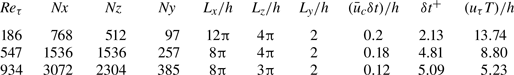
3.2.2. Comparisons of the estimation results from the GRBE and RBE
Like the case settings in the validations with the Ginzburg–Landau equation, three cases are set with different temporal resolutions, namely the TR, RS and TU cases. In the TR case, the sampled data are temporally resolved with  $\Delta t^+ = \delta t^+$, which corresponds to the case where the measured data are finely sampled in time and well restored. In the RS case, the sampling time intervals are uniformly distributed between $\Delta t^+ = \delta t^+$ and $32 \delta t^+$, as shown in figure 5. In this case, the temporal information is partially utilised, which corresponds to the case where the initially time-resolved measured data are missing arbitrarily. As for the TU case, the sampling interval is set as $\Delta t^+ = 32 \delta t^+$. Besides the sampling temporal intervals, the types of observed quantities may also influence the estimation accuracy. Meanwhile, in this section, we only show the estimation results from the observations of both the wall shear stress and pressure at the wall for brevity. On the other hand, detailed discussions on the impacts of choices of measurement types and the inclusion of forcing models on the estimation accuracy of the GRBE will be presented in the following § 4. The estimators of both RBE and GRBE are informed by the real flow statistics. With the above settings, the GRBE and RBE estimators are informed by abundant information, including all the considered wall quantities, i.e. wall shear stress and pressure, and exact flow statistics. Such choice enables us to adequately compare the performance of the two methods with given sampling time intervals of the measurement while excluding the influence from other factors.
Sampling time intervals in the RS case of turbulent channel flow with  $Re_{\tau }=934$.
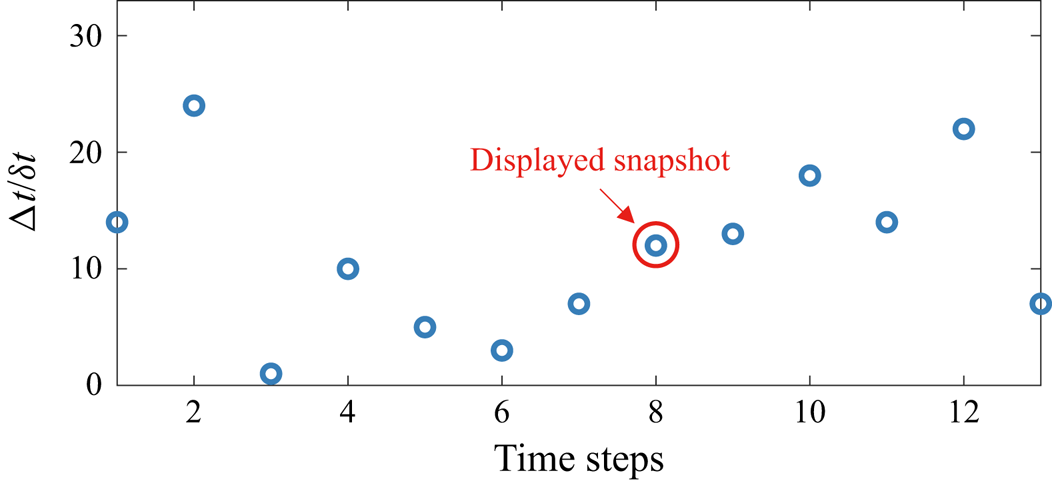
Intuitive insights into the estimation results can be found in the instantaneous flow field at  $y^+ = 100$ with $Re_{\tau } = 934$ shown in figure 6. It is observed that the estimation results from the GRBE and RBE are the same in the TR case. The estimated results from both approaches recover well the representative flow structures in the DNS results. With the increase of the sampling intervals, the estimation accuracy of the RBE rapidly deteriorates, where some non-physical small-scale spanwise streaks are observed, as in figure 6( f,g) in the RS and TU cases. In the meantime, although the flow structures estimated by the GRBE also become blurred a little in cases RS and TU, which is attributed to the decrease of measurement information, they still provide credible estimations of the large-scale structures.
Instantaneous flow state at  $y^+ = 100$ from the DNS results ( $a$), the GRBE results (b–d) and the RBE results (e–g). The sampling time intervals are set as temporally resolved (in the TR case) (b,e), randomly sampled (in the RS case) (c,f) and temporally unresolved (in the TU case) (d,g). The values shown in the figures are normalised by the maximum velocity fluctuation value in the DNS result.
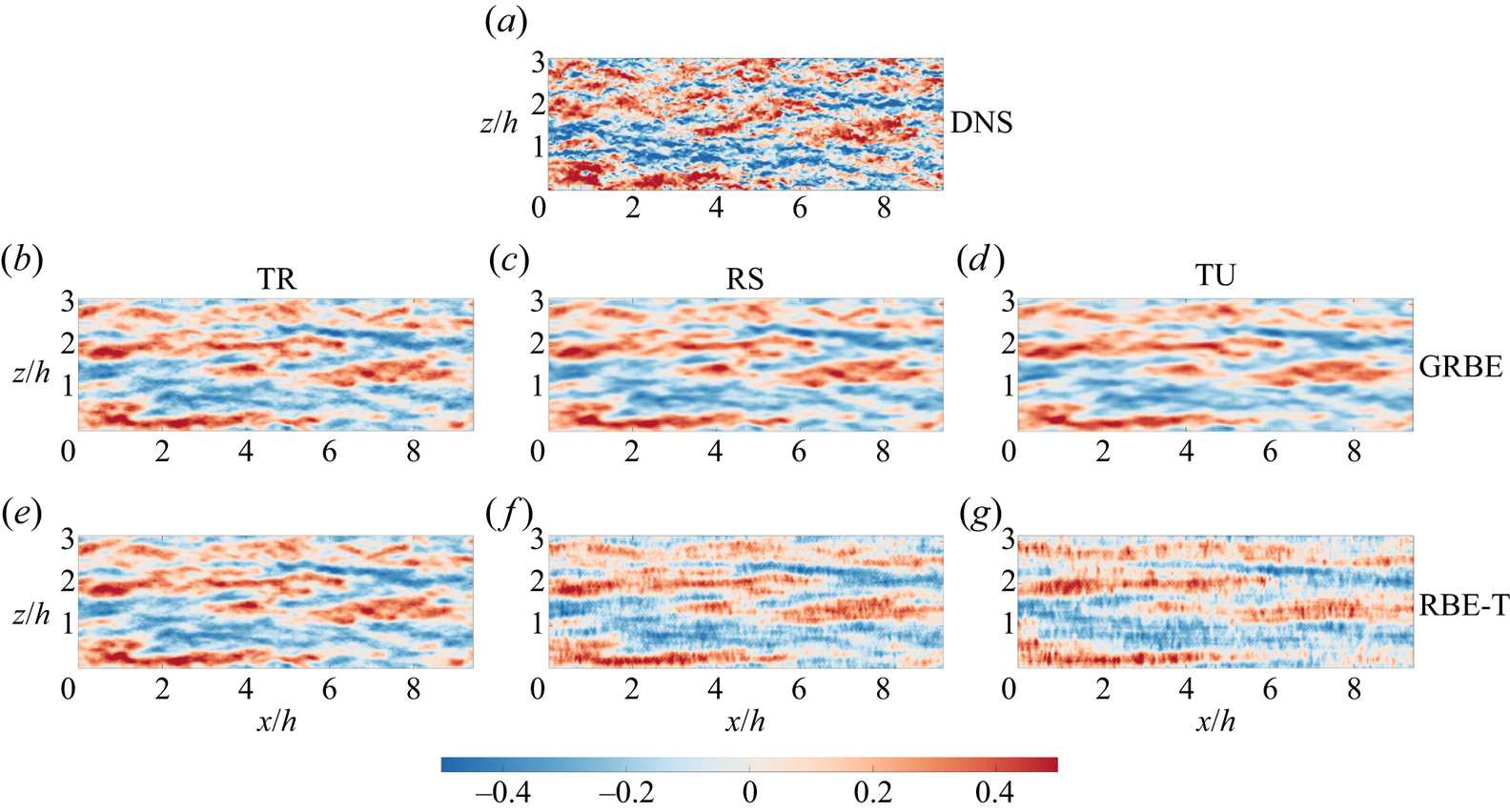
To quantitatively investigate the estimation accuracy of the GRBE and RBE results, the relative MSE for the estimated turbulent channel flow is defined as
 \begin{equation} {\rm Err}(y)=\frac{\left\langle \sum_{k_x}\sum_{k_z} \sum_t \hat{\varepsilon}(k_x,k_z,y,t) \bar{\hat{\varepsilon}}(k_x,k_z,y,t)\right\rangle }{ \left\langle \sum_{k_x}\sum_{k_z} \sum_t \hat{u}(k_x,k_z,y,t)\bar{\hat{u}}(k_x,k_z,y,t)\right\rangle }. \end{equation}
The profiles of the relative MSEs from the GRBE and RBE with different  $Re_{\tau }$ and sampling time intervals are shown in figure 7. In the TR case where $\Delta t = \delta t$, the curves denoting the estimation error from the GRBE and RBE overlap with each other, which again demonstrates that the GRBE is equivalent to RBE when the sampling time is resolved in time, as pointed out in § 2.4. When the sampling intervals are randomly distributed in the RS case, the estimation errors of the GRBE along the height slightly increase compared with those in the TR case due to the reduction of measurement information. Meanwhile, the estimation errors of the RBE in the RS case are much larger in comparison with those in the TR case. When the sampling time interval increases to $32 \delta t^+$ in the TU case, the estimation errors of the RBE results become even larger, while those from the GRBE maintain a relatively low magnitude. For instance, compared with the TR cases, the relative MSE from the RBE at $y^+ = 100$ with $Re_{\tau }=934$ increases by $43.7\,\%$ in the TU case, while that from the GRBE increases by only $10.1\,\%$.
Comparison of the relative MSEs from the RBE and GRBE with different measurement sampling intervals with  $Re_{\tau } = 186$ ( $a$), 547 ( $b$) and 934 ( $c$).
$c$).
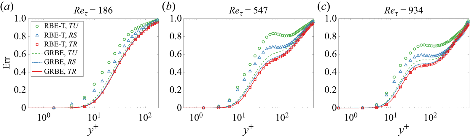
From the above comparisons between the estimation results from the RBE and GRBE, the GRBE is capable of providing a satisfying estimation for the turbulent channel flows with different sampling time intervals when the measurements are wall shear stress and pressure with real flow statistics informing the estimator.
4. Applications
In this section, the validated GRBE will continue to be applied in the estimations of turbulent channel flows to systematically investigate the characteristics of the GRBE in different application scenarios. In general, there are several related problems to be further uncovered, including (i) the influence of the abundance of the measured information on the estimation accuracy, including the amount of temporal information and sensor types, (ii) the Reynolds number effects and (iii) the performance of the forcing models when incorporated into the GRBE estimator. Discussions on the impacts of measurement abundance and Reyolds number effects are provided in § 4.1, while those on the impacts of the forcing models are presented in § 4.2.
4.1. Impacts of the abundance of measurement information on the estimation accuracy
The impact of different observation types, including wall shear stress and pressure, is preliminarily studied in Amaral et al. (Reference Amaral, Cavalieri, Martini, Jordan and Towne2021), leading to the conclusion that the estimation accuracy is improved with the increasing amount of the measured quantity types. Meanwhile, the problem becomes more complex when the abundance degree of temporal information is introduced. The variations of estimation accuracy with the measurement abundance at different flow scales also await further examination.
To investigate the impact of the abundance of temporal measurement information, three cases with different sampling temporal intervals are set, namely TU for the temporally unresolved case, RS for the randomly sampled case and TR for the temporally resolved case. Note that the sampling intervals in the TU case in this section are further enlarged to be  $240\delta t$, $160\delta t$ and $160\delta t$ for turbulent channel flows with $Re_{\tau } = 186$, 547 and 934, respectively, which are all the same as the lengths of the DNS data in temporal direction for each block with corresponding $Re_{\tau }$, as presented in § 3.2.1. This means that the flow information at only one snapshot is used for each TU case. On the other hand, to investigate the impacts of the sensor types on the estimation accuracy, different combinations of wall quantities, including the streamwise shear stress $\tau _u$, spanwise shear stress $\tau _w$ and pressure $p$, are also considered in this study. All of the to-be-tested combinations of the sampling intervals and sensor types in this study are summarised in table 2. In this section, the estimations with wall measurements informed by the real flow statistics are conducted.
Nomenclature of the cases testing the impacts of the sampling time intervals and sensor types on estimating the turbulent channel flow in this study.
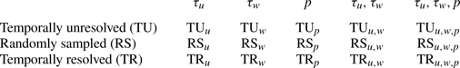
Instantaneous snapshots of the DNS result and the estimations at  $y^+ = 100$ with $Re_{\tau }=934$ are depicted in figure 8. Different types of sensors with various extents of temporal information are considered. In case TR $_{u,w,p}$ where the measured flow information is the most abundant, the GRBE estimator provides the most accurate results, where the flow structures recover well the representative ones in the DNS results. With the decrease of either the sensor types or temporal information, the estimated small flow structures become blurred. In case TU $_u$ with the least measured information, only the large-scale structures with long streaky structures could be observed. Interestingly, it is found that the flow structures are still well estimated in case TU $_{u,w,p}$ where the flow information at only one snapshot is used for the estimation. Compared with case TR $_{u}$ with measurements of $N_x \times N_z \times N_T$, the results from case TU $_{u,w,p}$ with $3 \times N_x \times N_z$ provide comparable flow information with a much lower requirement of measured data.
Estimated instantaneous flow state at  $y^+ = 100$ with measurements at the wall from the GRBE. The DNS result ( $a$) is presented as a reference. The measured quantities are set as $(\tau _u,\tau _w,p)$ (b–d), $(\tau _u,\tau _w)$ (e–g) and $\tau _u$ (h–j). The sampling time intervals are set as temporally resolved (b,e,h), randomly sampled (c,f,i) and temporally unresolved (d,g,j). The values shown in the figures are normalised by the maximum velocity fluctuation value in the DNS result.
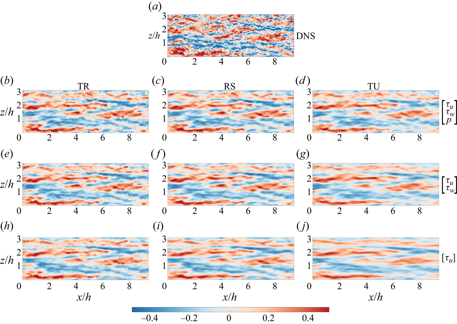
Next, we further investigate the impacts of the measurement abundance through the profiles of the relative MSEs. Figure 9 shows the profiles of the relative MSEs along the height. For all the tested  $Re_{\tau }$, it is observed that the estimation errors generally increase with the enlarged distance from the measurement location, i.e. the wall. At each height, the results in TR cases are the most accurate among those with the same sensor types. Meanwhile, case TU $_{u,w,p}$ that only needs the measured data at one instant has an even smaller error compared with case TR $_{u}$ that needs temporally resolved measurements when $y^+ < 100$. The Reynolds number effects on the GRBE accuracy can also be observed from figure 9. At a given height $y^+$, the estimation errors decrease with the enlargement of $Re_{\tau }$ for each case. For instance, at $y^+ = 100$, the estimation errors in case TR $_{u,w,p}$ are equal to 0.88, 0.60 and 0.48 when $Re_{\tau } = 186$, 547 and 934, respectively. In the meantime, an approximate plateau of the relative MSEs in the buffer zone is observed when $Re_{\tau } = 547$ and 934, which is more obvious with the higher $Re_{\tau }$. When $Re_{\tau } = 934$, the estimation errors even slightly decrease with the increase of height for cases with measurements of $\tau _u$.
Profiles of the relative MSEs of the streamwise velocity fluctuations from the GRBE in turbulent channel flows with  $Re_{\tau }=186$ ( $a$), 547 ( $b$) and 934 ( $c$).
$c$).
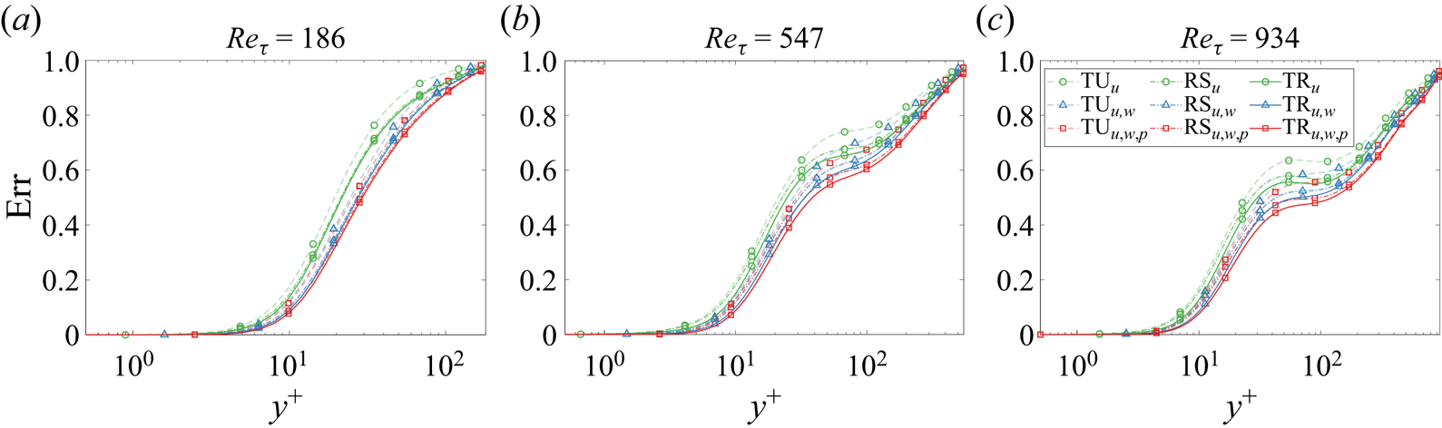
To further excavate the underlying mechanism of the differences in the estimation accuracy with different  $Re_{\tau }$, the relative estimation error energy as a function of $y$ and the flow scale $\lambda _x$ is defined by
 \begin{equation} {\rm Err}_x(\lambda_x , y) =\frac{\left\langle \sum_{k_z} \sum_t \hat{\varepsilon}(k_x,k_z,y,t) \bar{\hat{\varepsilon}}(k_x,k_z,y,t)\right\rangle }{ \left\langle \sum_{k_z} \sum_t \hat{u}(k_x,k_z,y,t)\bar{\hat{u}}(k_x,k_z,y,t)\right\rangle }, \end{equation}
where  $\lambda _x = 2 {\rm \pi}/ k_x$. As shown in figure 10, with the increasing flow scale, the estimation errors at a given height decrease monotonically. In the meantime, the plateaus in the estimation errors that are observed in the overall error energy profiles in figure 9(b,c) are much more obvious for the VLSMs ( $\lambda _x \geqslant 3h$) (Adrian, Meinhart & Tomkins Reference Adrian, Meinhart and Tomkins2000; Lee & Sung Reference Lee and Sung2013; Lee et al. Reference Lee, Lee, Choi and Sung2014) in the buffer zone. Especially, for the VLSMs with $\lambda _x = 4 {\rm \pi}$, the values of the estimation errors are around 0.18 at the plateaus at $y^+ = 40 \sim 100$ in case TR $_{u,w,p}$ with $Re_{\tau } = 934$. Meanwhile, for the motions with small scales of $\lambda _x \leqslant 3h$, the plateaus are not found in the buffer zone, which indicates that the nonlinear effects are stronger for such small-scale motions.
Relative MSEs of the streamwise velocity fluctuations from the GRBE in turbulent channel flows as functions of the flow scale  $\lambda _x^+$ and wall-normal distance $y^+$ in cases ${\rm TR}_{u,v,w}$ (a,c,e) and ${\rm TU}_u$ (b,d,f) with $Re_{\tau} = 934$ (a,b), 547 (c,d), and 186 (e,f). The blue curves denote the profiles of the relative MSEs for flow motions with given $\lambda^{+}_{x}$, while the red ones denote the contours of ${\rm Err}_x = 0.2$, 0.4, 0.6 and 0.8, respectively.
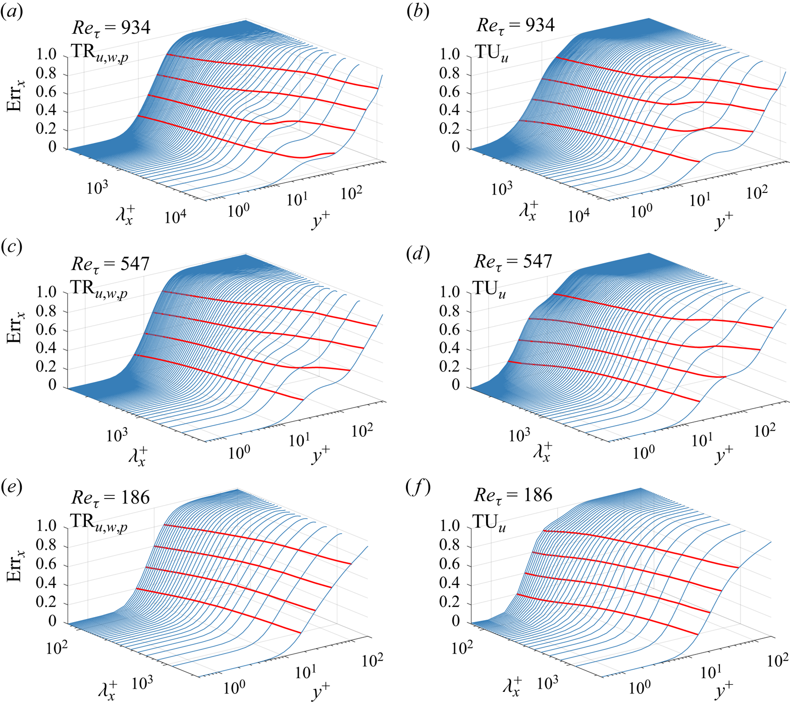
In the following, deeper investigations on the GRBE estimator are conducted by studying the two-dimensional energy spectra of the estimation and the corresponding energy distributions of the errors as functions of  $\lambda _x$ and $\lambda _z$. Similar to (4.1), the two-dimensional relative energy distribution of the estimation error at a given height $y_o$ is defined by
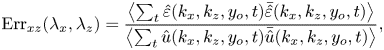 \begin{equation} {\rm Err}_{xz}(\lambda_x , \lambda_z) =\frac{\left\langle \sum_t \hat{\varepsilon}(k_x,k_z,y_o,t) \bar{\hat{\varepsilon}}(k_x,k_z,y_o,t)\right\rangle }{ \left\langle \sum_t \hat{u}(k_x,k_z,y_o,t)\bar{\hat{u}}(k_x,k_z,y_o,t)\right\rangle }, \end{equation}
where  $\lambda _x = 2 {\rm \pi}/ k_x$. The premultiplied spectra of estimated velocity fluctuation energy and the corresponding relative MSEs of $u$ at $y^+ = 40$ and 100 are shown in figures 11 and 12, respectively. To quantify the spectral region with relatively high estimation accuracy, the contours of $\textrm {Err}_{xz}(\lambda _x , \lambda _z) = 0.25$ and 0.75 in the corresponding figures are highlighted with white solid and dashed curves, respectively. Meanwhile, the scope of the self-similar attached eddies, i.e. $\lambda _x \geqslant 2\lambda _z$, $\lambda _x \geqslant 10y$, and $\lambda _z \geqslant 2y$, as suggested by Lozano-Durán, Flores & Jiménez (Reference Lozano-Durán, Flores and Jiménez2012), Hwang (Reference Hwang2015) and Cheng et al. (Reference Cheng, Li, Lozano-Durán and Liu2019), are also highlighted with black dot-dashed lines.
Premultiplied energy spectra ( $1\textrm {st}$ and $3\textrm {rd}$ panels) and the relative error energies ( $2\textrm {nd}$ and $4\textrm {th}$ panels) of $u$ at $y^+ = 40$ using the measurements at the wall. The sensor types are $\tau _u$, $\tau _w$, and $p$ (a–d), $\tau _u$ (e–h), $\tau _w$ (i–l) and $p$ (m–p). The black dot-dashed lines in each figure denote the range of the attached eddies. In the $1\textrm {st}$ and $3\textrm {rd}$ panels, the solid and dashed curves denote the contours of the energy spectra from DNS and estimations, respectively. In the $2\textrm {nd}$ and $4\textrm {th}$ panels, the contours of $\textrm {Err}_{xz} = 0.25$ and 0.75 are highlighted with white solid and dashed curves, respectively.

Same as figure 11, but at  $y^+ = 100$.
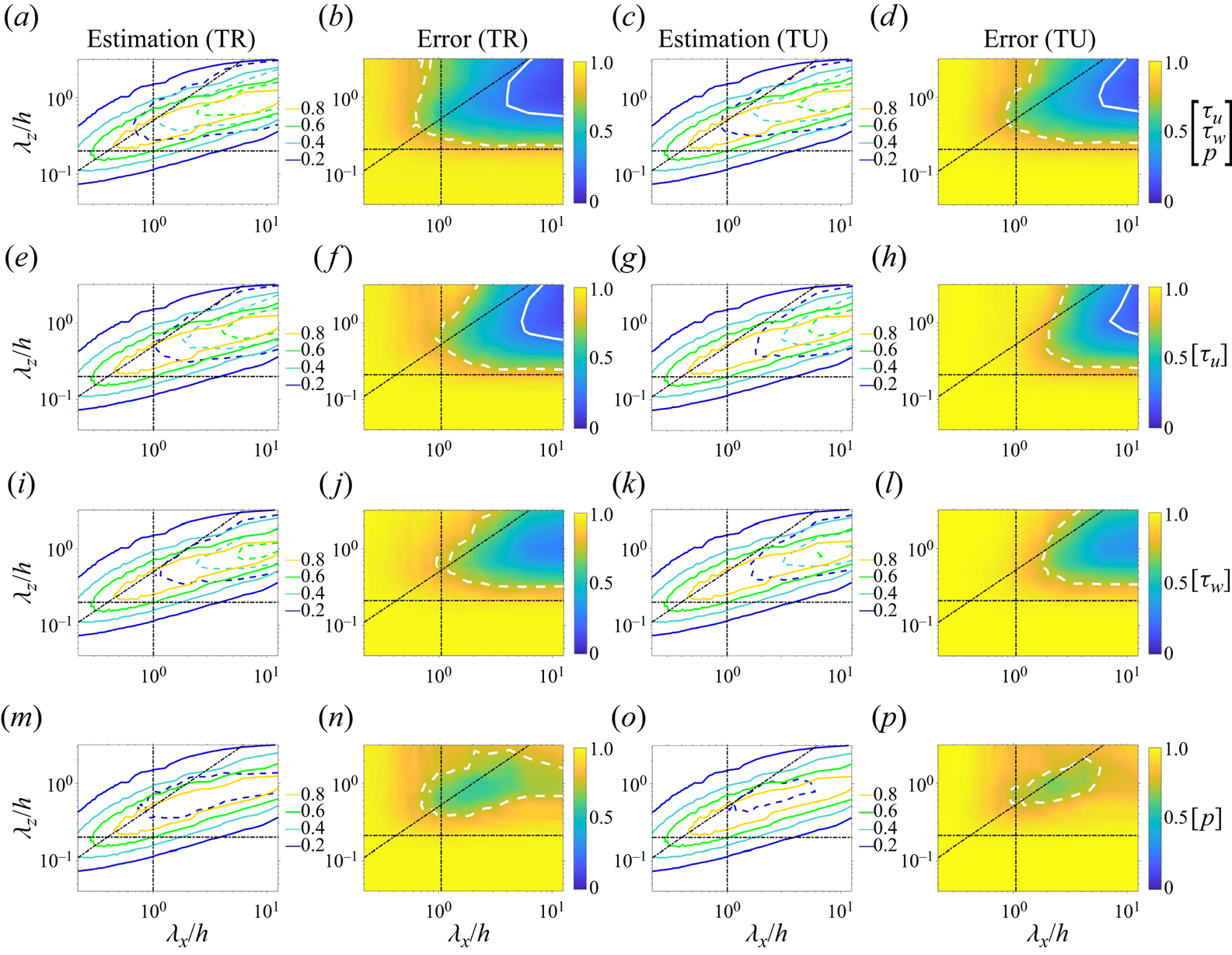
From figures 11 and 12, estimated premultiplied energy spectra in the dashed curves match relatively well with the DNS results within the spectral region corresponding to the attached eddies when the sensor types are  $\lbrace \tau _u,\tau _w,p \rbrace$ or $\lbrace \tau _u \rbrace$. Correspondingly, the relative energies of the estimation errors are generally smaller for the flow portions with larger wavelengths. On the other hand, the spectral regions where $\textrm {Err}_{xz} \leqslant 0.75$ at $y^+ = 40$ are much larger than those at $y^+ = 100$, which means that the estimation errors of the small-scale structures are significantly enlarged. Meanwhile, the extents of the regions where $\textrm {Err}_{xz} \leqslant 0.25$ for the large-scale flows do not shrink so obviously when the estimation layers lifts from $y^+ = 40$ to $y^+ = 100$. This phenomenon is consistent with the plateaus for the VLSMs existing at the buffer zones observed in figure 10.
The sensor types are found to have significant impacts on the energy distributions of the estimation errors in figures 11 and 12. Comparing the results in cases TR $_{u,w,p}$ and TR $_{u}$, obvious increases of the estimation errors are observed in the spectral region of $10y < \lambda _x < 2\lambda _z$. At $(\lambda _x / h , \lambda _z / h) = (0.36{\rm \pi}, {\rm \pi})$ on $y^+ = 40$, the value of the error energy is 0.52 and 0.94 in cases TR $_{u,w,p}$ and TR $_{u}$, respectively, with an increasing rate of $81.5\,\%$. On the other hand, at $(\lambda _x / h,\lambda _z / h) = (4{\rm \pi}, 0.5{\rm \pi} )$ inside the scope of the attached eddies, the error energy increases by $20.0\,\%$ in case TR $_u$ in comparison with that in case TR $_{u,w,p}$, which is not so dramatic as that at $(\lambda _x / h,\lambda _z / h) = (0.36{\rm \pi}, {\rm \pi})$. Besides the estimation results with measurements of $\lbrace \tau _u , \tau _w , p \rbrace$ and $\lbrace \tau _u \rbrace$, those with $\lbrace \tau _w \rbrace$ and $\lbrace p \rbrace$ are also shown in figures 11 and 12 to study the characteristics of the GRBE in cross-quantity estimation. In case TR $_{w}$, the region where $\textrm {Err}_{xz}(\lambda _x,\lambda _z) \leqslant 0.75$ that is surrounded by the white dashed lines is comparable to that in case TR $_{u}$, which roughly matches the range of the attached eddies. However, for large-scale flow motions, the estimation errors in case TR $_{w}$ are generally larger than 0.25, which is larger than those in TR $_{u}$. Thus, although the GRBE is capable of providing fair estimations of the small-scale structures of $u$ with measurements of $\tau _w$, the large-scale structures cannot be well estimated from cross-quantity estimations. In case TR $_{p}$ with wall pressure measurements, the estimation errors are obviously lower than those in the TR $_{u}$ case for the small-scale flows, which is beyond the scope of the attached eddies. For $(\lambda _x / h,\lambda _z / h) = (0.36{\rm \pi}, {\rm \pi})$ at $y^+ = 40$, the error energy in case TR $_{p}$ is $0.75$, which is $20\,\%$ lower than that in case TR $_{u}$. Meanwhile, for the estimations of large-scale structures, the GRBE in the TR $_{p}$ case is not as good as those in other cases.
Besides the sensor types, the abundance of the measurement temporal information is indeed another factor that influences the performance of the GRBE. Compared with cases TR $_{u,w,p}$ and TU $_{u,w,p}$, the reduction of the measured information in time reduces the estimation accuracy for all the considered spatial scales. Unlike the sensor types, which have significant influences on the patterns of the energy distributions of errors, the variations of the temporal information of measurements do not obviously change the error energy distributions. For instance, at $(\lambda _x,\lambda _z) = (0.36{\rm \pi}, {\rm \pi})$ and $(4{\rm \pi}, 0.5{\rm \pi} )$ on $y^+ = 40$ that are outside and inside the scopes of attached eddies, the value of the relative error energy increases by $46.2\,\%$ and $53.9\,\%$ in cases TU $_{u,w,p}$ compared with those in the TR $_{u,w}$ case, respectively, which are relatively close to each other.
To find out the performance of the GRBE with the variations of sampling intervals, we gradually increase the sampling time interval. The variations of the relative MSEs with the enlargement of the sampling intervals are shown in figure 13(a), while the increasing rate of the relative MSEs compared with those in the TR cases are shown in figure 13(b). For each combination of the sensor types, the estimation error does not obviously increase when  $\Delta t / \delta t \leqslant 5$. The relative deviations compared with the TR cases are no greater than $5\,\%$ until $\Delta t / \delta t$ increases to $16$ ( $\Delta t^+ = 81.41$). When $16 \leqslant \Delta t / \delta t \leqslant 80$, a relatively obvious increase in the estimation error with the enlarging sampling interval is observed. When the sampling intervals increase over $80 \delta t$, the estimation errors become almost unchanged with a further increase of $\Delta t$. For the estimations with measurements including $\tau _u$, the largest relative MSEs in the case with $\Delta t = 160 \delta t$ are around $15\,\%$ larger than the temporally resolved cases. Meanwhile, the errors of the cross-quantity estimation with measurements of $\lbrace \tau _w \rbrace$ and $\lbrace p\rbrace$ increase by around $8\,\%$ in TU cases compared with the TR ones. The relatively small increase in the cross-quantity estimation errors should be attributed to the fact that their magnitudes are already large in the TR cases, as shown in figure 13(a). In the meantime, it is noticed that the estimation error in case TU $_{u,w,p}$ is almost the same as that in the TR $_{u}$ case with a discrepancy of less than $1\,\%$.
Variations of the estimation error energies with measurement time intervals. ( $a$) Values of the relative MSEs. ( $b$) Variations of the relative MSEs compared with those in the TR cases with the corresponding measured quantities.

To further investigate the impact of sampling temporal intervals on the estimation accuracy, the increasing rates of the error energies compared with those in the TR cases as functions of measurement time intervals  $\Delta t$ and the streamwise wavelength $\lambda _x$ are depicted in figure 14. To quantify the impact of the increasing sampling temporal intervals on the estimation accuracy of flow motions with different scales, the threshold sampling interval $\Delta t_{T}$ is defined herein as the maximum sampling interval with which the increasing rate of $\textrm {Err}_x$ compared with the TR cases is smaller than $5\,\%$. For the attached eddies with $\lambda _x \geqslant 10y$, the threshold temporal interval $\Delta t_{T}$ is generally larger than $20 \delta t$, where $\Delta t_{T}^+ \geqslant 101.76$. On the other hand, when $3y \leqslant \lambda _x < 10y$, $\Delta t_{T}$ decreases with decreasing wavelength, which indicates that finer temporal resolution is required to provide effective information of the smaller flow scales. When $\lambda _x = 3y$ with the sensor of $\lbrace \tau _u , \tau _w , p \rbrace$, $\Delta t_{T}$ decreases to the minimum value of approximately $10 \delta t$. When the flow scales further decrease to $\lambda _x < 3y$, $\Delta t_{T}$ dramatically increases instead, which is attributed to the fact that the estimation errors with $\lambda _x < 3y$ are already near 1.0 in the TR cases, as shown in figure 10.
The increasing rate of the estimation error energies compared with those in the TR case as functions of sampling time intervals  $\Delta t$ and streamwise wavelengths $\lambda _x$ at $y^+ = 100$ with wall measurements of $\lbrace \tau _u , \tau _w , p \rbrace$ ( $a$),
$a$),  $\lbrace \tau _u \rbrace$ ( $b$),
$b$),  $\lbrace \tau _w \rbrace$ ( $c$) and $\lbrace p \rbrace$ ( $d$). The black dashed and solid lines denote the contours of $5\,\%$ and $15\,\%$, respectively.

From the above discussions, it can be concluded that the temporal information has limited impacts on the estimation accuracy, with a maximum reduction of around  $13.0\,\%$ of the estimation error in the TR case compared with the TU cases at $y^+ = 100$ with measurements of wall shear stress and pressure. When the sampling time intervals $\Delta t = 16 \delta t$ ( $\Delta t^+ = 81.41$), the increasing rates of the estimation errors are around $5\,\%$ compared with the TR results. Such findings indicate that the measurements with sparse samplings can be effectively used to provide reasonable estimations of the flow state with the GRBE. On the other hand, the inclusion of more types of observations can be efficient in improving the estimation accuracy. In the TU cases without temporal measurement information, the estimation error reduces by $12.3\,\%$ when the sensors for $\tau _w$ and $p$ are added besides that for $\tau _u$. Consequently, the relative MSEs at $y^+ = 100$ in the TU $_{u,w,p}$ case with the most sensor types but least temporal information are almost the same as those in the TR $_u$ case with the least sensor type but most temporal information.
Besides the above conclusions, we would also like to discuss the tolerated estimation error from the GRBE when applied in real engineering scenarios. Generally speaking, the feasibility of the GRBE depends on specific requirements on the estimation accuracy for a given range of flow scales. For instance, in flow control problems, the combination of sensors and actuators that are both limited to one wall-normal location provides a comparable control performance to the case where the limited-in-space actuators are informed by the entire flow information (Oehler & Illingworth Reference Oehler and Illingworth2021). This is due to the fact that the linear actuators are also limited by the flow coherence like the linear estimator, which means that the energy-containing LSMs could be better controlled. Since the GRBE provides reliable estimations of the large-scale structures in the inner layer, it can already well excavate the potentials of the linear actuator in controlling the large-scale turbulent flows. On the other hand, for the estimation problem of small-scale structures outside the scale range of the attached eddies, which is unresolved yet for all the current linear and nonlinear estimators (e.g. Guastoni et al. Reference Guastoni, Güemes, Ianiro, Discetti, Schlatter, Azizpour and Vinuesa2021) to the best of the authors’ knowledge, the GRBE is also not able to provide reliable results. Meanwhile, since GRBE has been validated to be the optimal linear estimator, the comprehensive discussions in this section are meaningful to evaluate the reliability and quantify the uncertainties of the linear estimation results in engineering applications.
4.2. Performance of the forcing models in flow state estimation
In the above, the performance of the GRBE estimators informed by the real flow statistics under different cases is discussed. Thus, no matter how the performance varies in different cases, they are already the optimal linear estimators with given measurements. In practice, the flow statistics are not always available when estimating the flow state, where the forcing models that predict the spatio-temporal statistical properties of turbulent flows are needed to inform the GRBE estimator. Thus, it is important to clarify their performance when informing the linear estimator of GRBE. In the following, three existing forcing models that provide spatio-temporal descriptions of the forcing statistics, including the B-model (Hwang & Cossu Reference Hwang and Cossu2010; Madhusudanan et al. Reference Madhusudanan, Illingworth and Marusic2019), W-model and  $\lambda$-model (Gupta et al. Reference Gupta, Madhusudanan, Wan, Illingworth and Juniper2021), will be applied to inform the GRBE estimator. Mathematical descriptions of these three models are provided in Appendix B. Estimation results with the wall measurements will be used for the discussions in this section.
Figure 15 shows the estimation errors of different forcing models with different sensor types along the wall-normal direction. Moreover, to provide intuitive results, figures 16, 17 and 18 show the instantaneous flow states estimated by GRBE estimators that are informed by the B-model, W-model and  $\lambda$-model, respectively. In the TU case, the W-model-informed GRBE provides the most accurate results, which are closer to the optimal linear estimated results than those from the other models. In case TU $_u$, the estimation error in the W-model-informed result at $y^+ = 100$ is $13.3\,\%$ larger than that from the optimal linear estimations, as in figure 15(b). From figure 17(d,g,j), it is also observed that the estimated large-scale structures from the W-model match well with the DNS results in the TU cases. Such good agreement between the W-model-informed result and the optimal linear result in case TU $_u$ indicates that the W-model can effectively predict the spatial coherence of the streamwise velocity between the wall and the higher region. Compared with the estimation errors from the W-model and $\lambda$-model, those from the B-model are obviously larger in the near-wall region of $y^+ \leqslant 10$. Meanwhile, with the increase of estimation height, the errors from the $\lambda$-model rapidly increase and exceed those from the B-model where $y^+ \geqslant 15$. On the other hand, the estimation error from each forcing model does not obviously decrease with the increase of sensor types. When converting the sensor types from $\lbrace \tau _u \rbrace$ to $\lbrace \tau _u, \tau _w, p \rbrace$, the estimation errors at $y^+ = 100$ decrease by $0.7\,\%$, $3.9\,\%$ and $8.0\,\%$ for the B-model, W-model and $\lambda$-model, respectively, which are lower than the value of $13.3\,\%$ by the optimal linear estimator. The relatively low efficiency of the forcing-model-informed GRBE estimator to improve the estimation accuracy with an increasing number of measured variables is attributed to the fact that all the tested forcing models cannot effectively predict the covariance between different quantities.
Variations of the estimation errors from the B-model (a,d,g), W-model (b,e,h) and  $\lambda$-model (c,f,i) with the wall-normal height in the TU (a–c), RS (d–f) and TR (g–i) cases. The scattered symbols and translucent curves denote the estimation results from the GRBE estimator incorporating the forcing models and real flow statistics, respectively.
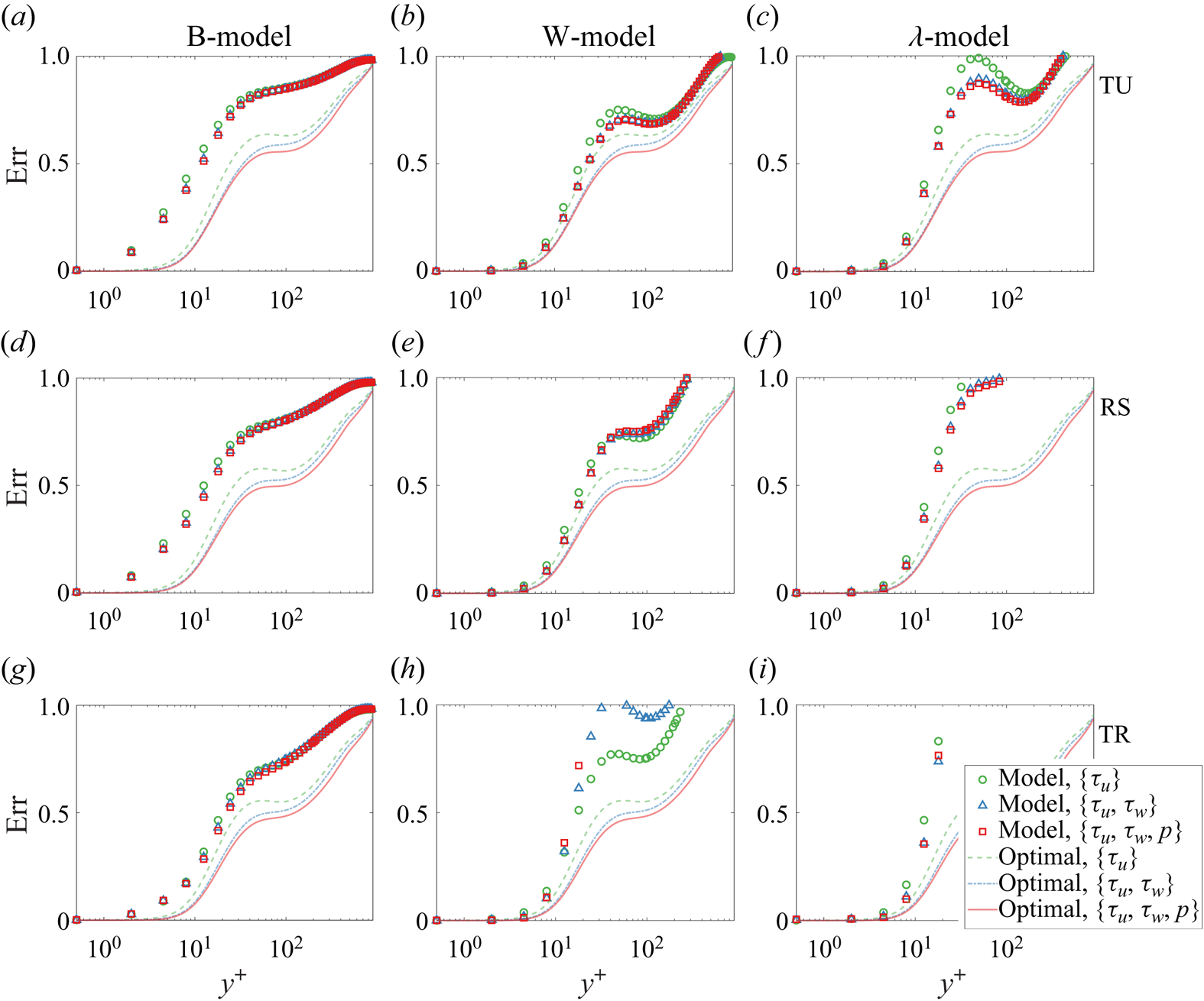
Estimations of the flow state with the B-model-informed estimator. The depicted figures are reference DNS result ( $a$); estimations with measurements of wall shear stress and pressure (b–d), wall shear stress (e–g) and streamwise wall shear stress (h–j). The measurements are temporally resolved (b,e,h), randomly sampled (c,f,i) and temporally unresolved (d,g,j). The values shown in the figures are normalised by the maximum velocity fluctuation value in the DNS result.
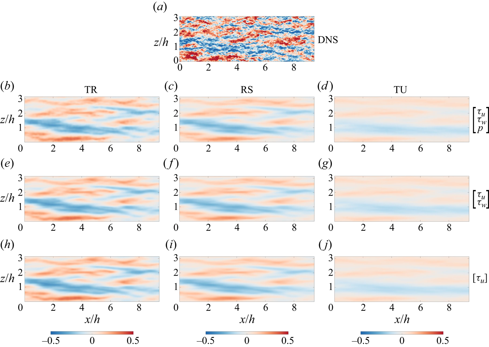
Same as figure 16, but with the W-model-informed estimator.
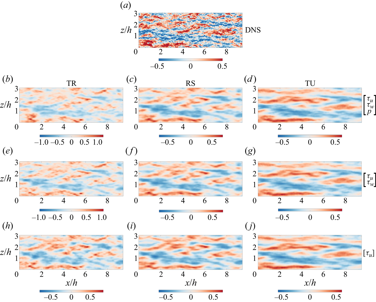
Same as figure 16, but with the  $\lambda$-model-informed estimator.

With the increase of the temporal information of measurements, it is interesting to find that the estimation errors from the W-model- and  $\lambda$-model-informed estimators increase accordingly, the tendencies of which are opposite to those of the optimal linear estimator. In the TR $_{ u, w, p}$ case, where the estimation error is minimised in the optimal linear estimator, it is instead maximised for the W-model results, which are $48.9\,\%$ larger than that in case TU $_{u, w, p}$. A similar non-physical phenomenon is observed in the $\lambda$-model results. From figures 17(a) and 18(a), the fluctuation energy of small-scale structures is incorrectly amplified by the W- and $\lambda$-models in the TR cases compared with the estimated results in the TU cases. Such non-physical increase of estimation error with the increase of temporal measurement information and sensor types indicates that the W-model and $\lambda$-model cannot effectively predict the temporal properties, although the W-model works well in predicting the spatial coherence of the streamwise velocity. On the other hand, the estimation errors of the B-model results decrease monotonically with the increase of the measurement abundance. Compared with the relative MSE in case TU $_{u,w,p}$ at $y^+ = 100$, that in case TR $_{u,w,p}$ decreases by $13.2\,\%$ from the B-model results.
In summary, the tested forcing models perform differently in cases with different measurement abundance. In case TU $_u$ with the least measurement information, the W-model performs the best. When the sensor types increase from $\lbrace \tau _u \rbrace$ to $\lbrace \tau _u, \tau _w, p \rbrace$, the estimation accuracy of the tested forcing models is not obviously improved. Moreover, with the increase of temporal information, the estimation errors from the W-model and $\lambda$-model non-physically increase. Such tendencies are opposite to those in the optimal linear estimation results, indicating that the temporal properties predicted by the W-model and $\lambda$-model cannot effectively reflect these of the real turbulence. A forcing model that properly models the forcing in the temporal domain will effectively improve the linear estimation accuracy of the GRBE without the requirement of the real flow statistics, which is to be explored in the future.
5. Conclusions
In this study, the RBE that estimates the turbulence field with temporally resolved measurement data is generalised so that credible linear estimations of the flow state can be obtained when the measurement data are arbitrarily sampled in time. The generalised version of RBE is named the GRBE herein. Unlike the RBE that minimises the expected error energy at each frequency, the transfer kernel of the GRBE is constructed with the target of directly minimising the expected error energy in physical space, by means of finding the stationary point of the MSE as a quadratic function of the transfer kernel. The flow statistics, including the CSD tensors of the forcing and measurement noise, are considered when constructing the GRBE estimator. In cases where the flow statistics are unavailable, the GRBE enables the incorporation of the forcing models that provide spatio-temporal predictions of the flow statistics.
Validations of the GRBE approach include the one-dimensional complex Ginzburg–Landau equation and turbulent channel flows with  $Re_{\tau }=186$, 547 and 934. The estimation results from the original RBE (Martini et al. Reference Martini, Cavalieri, Jordan, Towne and Lesshafft2020; Towne et al. Reference Towne, Lozano-Durán and Yang2020) and the $H_2$-optimal estimation (Doyle et al. Reference Doyle, Glover, Khargonekar and Francis1989; Illingworth et al. Reference Illingworth, Monty and Marusic2018) are also included in the case of the complex Ginzburg–Landau equation. When the measurement information is resolved in the temporal direction, the GRBE results are equivalent to those from the RBE. As the sampling time intervals arbitrarily increase, the relative MSEs of the GRBE results still keep relatively low magnitudes, while those of the RBE are obviously enlarged when the sampling time intervals increase. The GRBE also provides the optimal results in causal estimations by comparing with the $H_2$-optimal estimation results. In the validation cases with the turbulent channel flows with $Re_{\tau } = 186$, 547 and 934, the measured signals are set to be the shear stress and pressure at the wall, with the real flow statistics incorporated in the GRBE and RBE estimators. The results of the GRBE and RBE are the same when $\Delta t^+ = \delta t^+ = 5.09$, i.e. the measurements are well resolved in time. When the sampling time intervals $\Delta t^+$ increase to $32 \delta t^+$, the estimation errors of the RBE are obviously enlarged, while those from the GRBE maintain relatively low magnitudes.
After validations, the GRBE is further utilised to comprehensively investigate its performance in different measuring conditions, where the factors influencing the estimation accuracy include the abundance of temporal measurement information and sensor types, as well as the Reynolds number effects. With the increase of  $Re_{\tau }$, the relative MSE at a given height decreases accordingly, where the plateaus of the relative MSE magnitudes are observed in the buffer zone when $Re_{\tau } = 547$ and 934. Investigations on the estimation errors with different streamwise scales $\lambda _x$ reveal that the plateaus mainly appear in the VLSMs, which are more energetic when $Re_{\tau }$ increases. By increasing the measurement types, the estimation accuracy of the turbulence state can be effectively improved. For instance, the relative MSE reduces by $12.3\,\%$ when the additional measurements of $\tau _w$ and $p$ are added to the original estimations where $\tau _u$ is measured in the temporally resolved case. On the other hand, increasing the temporal information of the measurements can also reduce the estimation error. When measuring the wall shear stress and pressure, the relative MSE at $y^+ = 100$ with $Re_{\tau } = 934$ decreases by $13.0\,\%$ in the TR case compared with the TU case with only spatial measurements.
Finally, the current spatio-temporal forcing models, including the B-model, W-model and  $\lambda$-model, are incorporated into the GRBE estimator to investigate the performances of these existing models when conducting the linear estimation. The estimated results with wall measurements are investigated to test the abilities of the existing forcing models in turbulence state estimation. The estimation errors from the W-model-informed estimator are relatively low in the TU cases, where the estimation error at $y^+ = 100$ in case TU $_u$ is only $13.3\,\%$ larger than that from the optimal linear estimations. This indicates that the W-model-predicted spatial statistics of turbulence reflect well the DNS results. However, for the TR cases, the estimation errors in the results from the W-model and $\lambda$-model non-physically increase, especially for the estimations with multiple types of observations. Thus, given a forcing model that provides a fair prediction of the spatial covariance of turbulence, its prediction accuracy on the temporal information is not guaranteed, and it might induce huge errors for state estimation. This highlights the importance of proper modelling strategies of forcing in the temporal domain.
When applied to experiments or engineering scenarios, the flow patterns and sensor locations may not be the same as those in this study. In such cases, the resolvent operator and, correspondingly, the GRBE transfer kernel, should be tuned to match the specific flow configuration and sensor layouts. More importantly, an appropriate forcing model should be incorporated in the GRBE framework such that the linear relationships between the measurement and estimations are properly evaluated in the given application scenario. With continuous studies on the colour of forcing in the frequency domain (e.g. Zare et al. Reference Zare, Chen, Jovanović and Georgiou2016, Reference Zare, Georgiou and Jovanović2020; Morra et al. Reference Morra, Nogueira, Cavalieri and Henningson2021; Nogueira et al. Reference Nogueira, Morra, Martini, Cavalieri and Henningson2021), an advanced forcing model that provides a more accurate description of the spatio-temporal properties of turbulence is promising to be proposed in the future, which will make the GRBE a more powerful tool in estimating the turbulence.
Funding
L.F. acknowledges the fund from the Research Grants Council (RGC) of the Government of Hong Kong Special Administrative Region (HKSAR) with RGC/ECS Project (no. 26200222), RGC/GRF Project (no. 16201023) and RGC/STG Project (no. STG2/E-605/23-N), the fund from Guangdong Basic and Applied Basic Research Foundation (no. 2024A1515011798), the fund from Guangdong Province Science and Technology Plan Project (no. 2023A0505030005), the fund from Center for Ocean Research in Hong Kong and Macau, a joint research center between Laoshan Laboratory and HKUST and the fund from the Project of Hetao Shenzhen–Hong Kong Science and Technology Innovation Cooperation Zone (no. HZQB-KCZYB-2020083).
Declaration of interests
The authors report no conflict of interest.
Data availability
The data that support the findings of this study are available on request from the corresponding author, L.F.
Appendix A. The spatial linearised Navier–Stokes operator
The spatial linearised NS operator  $\mathcal {L}_{\boldsymbol {k}_{s}} \in \mathbb {C}^{3N_y \times 3N_y}$ in (2.8a–c) for the momentum equations is calculated as
 \begin{equation} \mathcal{L}_{\boldsymbol{k}_{s}} = \boldsymbol{\mathsf{L}}_0 + {\rm i}{k_x}{\boldsymbol{\mathsf{L}}_x} + {\boldsymbol{\mathsf{L}}_y} \mathscr{D} + {\rm i}{k_z}{\boldsymbol{\mathsf{L}}_z} + {\boldsymbol{\mathsf{L}}_2}(- k_x^2 + \mathscr{D}^2 - k_z^2), \end{equation}
with
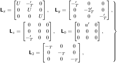 \begin{equation} \left.\begin{gathered} \boldsymbol{\mathsf{L}}_x = \left[ \begin{array}{@{}ccc@{}} U & -\mathscr{v}_T^{\prime} & 0 \\ 0 & U & 0 \\ 0 & 0 & U \end{array} \right], {\quad} \boldsymbol{\mathsf{L}}_y = \left[ \begin{array}{@{}ccc@{}} -\mathscr{v}_T^{\prime} & 0 & 0 \\ 0 & -2\mathscr{v}_T^{\prime} & 0 \\ 0 & 0 & -\mathscr{v}_T^{\prime} \end{array} \right],\\ \boldsymbol{\mathsf{L}}_z = \left[ \begin{array}{@{}ccc@{}} 0 & 0 & 0 \\ 0 & 0 & 0 \\ -\mathscr{v}_T^{\prime} & 0 & 0 \end{array} \right], {\quad} \boldsymbol{\mathsf{L}}_0 = \left[ \begin{array}{@{}ccc@{}} 0 & u^{\prime} & 0 \\ 0 & 0 & 0 \\ 0 & 0 & 0 \\ \end{array} \right],\\ \boldsymbol{\mathsf{L}}_2 = \left[ \begin{array}{@{}ccc@{}} -\mathscr{v}_T & 0 & 0 \\ 0 & -\mathscr{v}_T & 0 \\ 0 & 0 & -\mathscr{v}_T \end{array} \right], \end{gathered}\right\} \end{equation}
where  $U$ is the mean streamwise velocity profile, $\mathscr {v}_T = ({1}/{Re_{\tau }})( {\nu _T}/{\nu })$, $\mathscr {D}$ and ${}^{\prime }$ denote ${\partial } / {\partial y}$. The Hamiltonian operator $\boldsymbol {\nabla } \in \mathbb {C}^{N_y \times 3N_y}$ in (2.8a–c) is calculated as
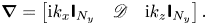 \begin{equation} \boldsymbol{\nabla} = \left[ {\rm i}{k_x}\boldsymbol{\mathsf{I}}_{N_y} \quad \mathscr{D} \quad {\rm i}{k_z}\boldsymbol{\mathsf{I}}_{N_y} \right]. \end{equation}
 The observation matrix  $\boldsymbol{\mathsf{C}}$ in (2.7b) is determined by the location of the measured variable. For instance, denoting $( u_1,u_2,u_3 ) = ( u,v,w )$, if the measured variable is the velocity $u_i~(i=1,2,3)$ at the $n$th node, then the observation matrix $\boldsymbol{\mathsf{C}} \in \mathbb {C}^{1 \times 4N_y}$ should be expressed as
 \begin{equation} \boldsymbol{\mathsf{C}} = \left[ \boldsymbol{\mathsf{O}}_{1 \times \left[ {(i-1)N_y + n-1}\right]} \quad 1 \quad \boldsymbol{\mathsf{O}}_{ 1 \times \left[{4N_y-(i-1)N_y-n}\right]} \right]. \end{equation}
Appendix B. The spatio-temporal forcing models
The concept of the spatio-temporal forcing model defined in this study refers to the method that provides the statistical description of forcing in both the wall-normal and temporal directions at each spatial scale  $\boldsymbol {k}_{s}$. Such spatio-temporal forcing models can be incorporated in the GRBE transfer function $\boldsymbol{\mathsf{h}}$ as in (2.18) when the measurements are unresolved in time. The existing methods that belong to the spatio-temporal forcing models include the B-model (Hwang & Cossu Reference Hwang and Cossu2010), W-model and $\lambda$-model (Gupta et al. Reference Gupta, Madhusudanan, Wan, Illingworth and Juniper2021). All these three models assume that the forcing is white in time and uncorrelated along the wall-normal direction. This means that the CSD tensors of the forcing at a given spatial scale $\boldsymbol {k}_{s}$ are diagonal and unchanged all over the frequencies $\omega$. The B-model specifies the forcing energy $E_{(\boldsymbol {k}_{s},\omega )}$ to be unchanged along the height, i.e.
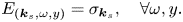 \begin{equation} E_{(\boldsymbol{k}_{s},\omega,y)} = {\sigma}_{\boldsymbol{k}_{s}},\quad \forall \omega,y. \end{equation}
With such a precise description of the forcing, the B-model is widely applied in relevant studies (Hwang & Cossu Reference Hwang and Cossu2010; Madhusudanan et al. Reference Madhusudanan, Illingworth and Marusic2019; Gupta et al. Reference Gupta, Madhusudanan, Wan, Illingworth and Juniper2021).
Extended from the work of Jovanović & Bamieh (Reference Jovanović and Bamieh2005) in laminar flow, the W-model (Gupta et al. Reference Gupta, Madhusudanan, Wan, Illingworth and Juniper2021) assumes that the vertical profile of forcing energy is proportional to that of the eddy viscosity, i.e.
 \begin{equation} E_{(\boldsymbol{k}_{s},\omega,y)} ={\sigma}_{\boldsymbol{k}_{s}} \nu_t^2(y), \quad \forall \omega,y. \end{equation}
 Considering that the nonlinear interactions of turbulence are scale dependent (Cho, Hwang & Choi Reference Cho, Hwang and Choi2018), the  $\lambda$-model (Gupta et al. Reference Gupta, Madhusudanan, Wan, Illingworth and Juniper2021) is further proposed with the modified eddy viscosity, i.e.
 \begin{equation} \nu_{t,{\boldsymbol{k}_{s}}}(y) = \frac{\lambda}{\lambda + \lambda_m(y)} \nu_t (y), \end{equation}
where  $\lambda = 2{\rm \pi} / (k_x^2 + k_z^2)^{0.5}$, and $\lambda _m (y) = 50/{Re_\tau }+(2-50/{Re_\tau }) \,\textrm {{tanh}} (6(1-\left|1-\tilde{y}\right|))$. The forcing energy profile is thereby calculated by
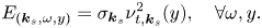 \begin{equation} E_{(\boldsymbol{k}_{s},\omega,y)} = {\sigma}_{\boldsymbol{k}_{s}} \nu_{t,\boldsymbol{k}_s}^2 (y),\quad \forall \omega,y. \end{equation}
Appendix C. Analyses of the estimation errors from the RBE in temporally unresolved cases
In this section, the estimation errors from the RBE-F and RBE-T approaches in the TU cases will be analysed. The estimation errors on different frequency bands will be separately investigated to study how the estimation errors are induced from the RBE approaches due to spectrum aliasing. The flow motions on each frequency band are firstly extracted from the original flow signal with high temporal resolution, then separately used for estimation in the TU case after down-sampling. To facilitate the following discussions, we denote P $i$ to be the frequency band with $\omega \in [(2n_i-1)\omega _{N},(2n_i+1)\omega _{N}]$, where $n_i = 0,-1,1,-2,2,\ldots$ for $i = 1,2,3,4,5,\ldots$, respectively, and $\omega _{N}$ is the Nyquist frequency. Two cases, including the one-dimensional Ginzburg–Landau equation and turbulent channel flow with $Re_\tau =934$ with temporally unresolved measurements, will be included in the discussions in this section. Settings of the sampling intervals in the TU cases can be found in §§ 3.1 and 3.2 for the Ginzburg–Landau equation and turbulent channel flows, respectively.
C.1. The one-dimensional Ginzburg–Landau equation
Firstly, the spectrum aliasing due to the under-sampling of the measurement data is investigated, which induces the estimation errors in the RBE-F results. Since the RBE-F uses the Fourier series directly from the DFT to conduct the estimations, the flow motions with  $\omega =\omega _{{P}1} + 2n_i\omega _{N}$ are identified to have a frequency of $\omega _{{P}1}$, where $| \omega _{{P}1} | \leqslant \omega _{N}$ (Karban et al. Reference Karban, Martini, Jordan, Brès and Towne2022). As a result, the flow motions with $\omega =\omega _{{P}1} + 2n_i\omega _{N}$ ( $n_i \ne 0$) are incorrectly estimated by RBE-F with the transfer function for $\omega _{{P}1}$. As shown in figure 19, the under-sampled spectrum in the TU case obviously differs from the original spectra. In figure 20(a), the relative MSE in the RBE-F result corresponding to frequency band P1 with lowest frequencies is the same as that from the optimal GRBE/RBE results in the TR case, and both are lower than the GRBE results in the TU case. This is due to the fact that the RBE-F constructs the transfer function according to P1, while the GRBE comprehensively considers the overall statistics across all the scales. Meanwhile, for the frequency bands with higher frequencies, the relative MSEs from the RBE-F rapidly increases to be larger than unity, which means that the optimal transfer function for band P1 is not effective for the other frequency bands with different frequencies.
Sketch of spectrum aliasing due to down-sampling of the measurement signal at  $x=10$ of the Ginzburg–Landau equation in the TU case. Grey curve: the original spectrum without aliasing; red curve: the measured spectrum with aliasing; blue curves: the piecewise spectra, with colour shades indicating the numbers of the frequency bands.
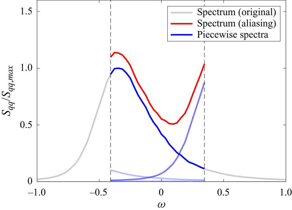
Relative MSEs at  $x=10$ for different frequency bands of the Ginzburg–Landau equation in the TU case. ( $a$) The estimation error at separated frequency bands. ( $b$) The accumulated estimation error by sequentially increasing the considered numbers of frequency bands.
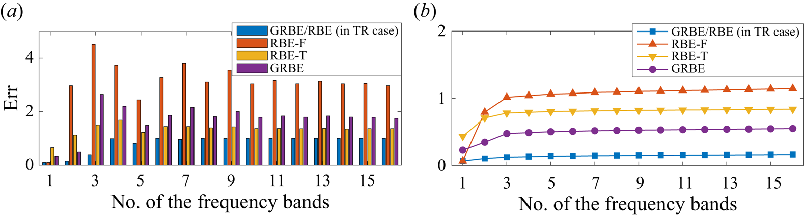
On the other hand, the RBE-T uses the discretised temporal transfer kernel by integration of the transfer kernel in the temporally resolved case, as shown in (2.30). From figure 20(a),the relative MSE of RBE-T at frequency band P1 is the largest one among those from the other methods. For the sequential frequency bands, the estimation errors of the RBE-T approach appear to be lower than those of the RBE-F approach. Meanwhile, both the RBE-F and RBE-T results have larger estimation errors than the GRBE approach when considering the summation of flow motions at all the frequency bands.
Appendix D. The  $H_2$-optimal estimation

The  $H_2$-optimal estimation (Illingworth et al. Reference Illingworth, Monty and Marusic2018) originates from the $H_2$-optimal control problem (Zhou & Doyle Reference Zhou and Doyle1998), where the term ‘ $H_2$’ is from the $H_2$ norm that is used to define the cost function in this problem. The $H_2$ norm of a stable matrix $M(s)$ is defined by
 \begin{equation} \| M \|_2 := \left( \frac{1}{2 {\rm \pi}} \int_{-\infty}^{\infty} {\rm Tr} \left[ M({\rm i}\omega) M({\rm i}\omega)^{{\ast}} \right] {\rm d}\omega \right)^{{1}/{2}}. \end{equation}
Now consider a dynamic system with the state evolution equation expressed by
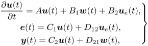 \begin{equation} \left.\begin{gathered} \frac{\partial \boldsymbol{u}(t)}{\partial t}= A\boldsymbol{u}(t) + B_1 {\boldsymbol{w}}(t) + B_2 {\boldsymbol{u}}_{e}(t), \\ \boldsymbol{e}(t) = C_1 \boldsymbol{u}(t) + D_{12} {\boldsymbol{u}}_{e}(t), \\ \boldsymbol{y}(t) = C_2 \boldsymbol{u}(t) + D_{21} {\boldsymbol{w}}(t), \end{gathered}\right\} \end{equation}
where  $\boldsymbol {u}$ is the state variable; $\boldsymbol {u}_{e}$ is the control input, which corresponds to the estimation for the optimal estimation problems; $\boldsymbol {w}$ is the spatio-temporally white external input, which includes the effects of disturbances, i.e. nonlinear forcing and sensor noise. Note that the cross-spectra of nonlinear forcing and the sensor noise are defined with $\boldsymbol {w}$ along with the matrices of $\boldsymbol {\mathcal {B}}$ and $\boldsymbol {\mathcal {D}}$ introduced below. Here, $\boldsymbol {e}$ is the output of the closed-loop system, which corresponds to the estimation error for the optimal estimation problems and $\boldsymbol {y}$ is the measurement. A diagram of the closed-loop system is shown in figure 21, where $G(s)$ denotes the state-space representation of
 \begin{equation} G(s)= \left[\begin{array}{c|c} A & B\\ \hline C & D\\ \end{array}\right] = C\left( s \boldsymbol{\mathsf{I}} - A \right)^{{-}1} B + D, \end{equation}
with
 \begin{equation} B=\left[B_1 \quad B_2\right],\quad C=\left[\begin{array}{c} C_1 \\ C_2 \end{array} \right],\quad D=\left[\begin{array}{cc} \boldsymbol{\mathsf{O}} & D_{12} \\ D_{21} & \boldsymbol{\mathsf{O}} \end{array} \right]. \end{equation}
The transfer matrix  $G(s)$ actually defines the linear relationship between $[ \boldsymbol {e}, \boldsymbol {y} ]^\textrm {T}$ and $[ \boldsymbol {w} , \boldsymbol {u}_{e} ]^\textrm {T}$ after taking Laplace transforms along the temporal direction, i.e.
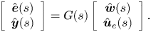 \begin{equation} \left[\begin{array}{c} \hat{\boldsymbol{e}}(s) \\ \hat{\boldsymbol{y}}(s) \end{array} \right] =G(s)\left[\begin{array}{c} \hat{\boldsymbol{w}}(s) \\ \hat{\boldsymbol{u}}_{e}(s) \end{array} \right]. \end{equation}
For output estimation problems, with respect to the parameters in (2.7), the linear operators and the external input  $\boldsymbol {w}$ in (D2) are given by
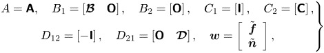 \begin{equation} \left.\begin{gathered} A=\boldsymbol{\boldsymbol{\mathsf{A}}},\quad B_1=\left[\boldsymbol{\mathcal{B}} \quad \boldsymbol{\mathsf{O}}\right], \quad B_2=\left[\boldsymbol{\mathsf{O}}\right],\quad C_1=\left[\boldsymbol{\mathsf{I}}\right],\quad C_2=\left[\boldsymbol{\mathsf{C}}\right], \\ D_{12}=\left[ -\boldsymbol{\mathsf{I}} \right],\quad D_{21}=\left[ \boldsymbol{\mathsf{O}} \quad \boldsymbol{\mathcal{D}} \right],\quad \boldsymbol{w}=\left[\begin{array}{c} \tilde{\boldsymbol{f}} \\ \tilde{\boldsymbol{n}} \end{array} \right], \end{gathered}\right\} \end{equation}
where  $\boldsymbol {\mathcal {B}}$ and $\boldsymbol {\mathcal {D}}$ are obtained from the Cholesky decompositions of the CSD tensors of forcing and measurement noise, respectively, i.e. $\boldsymbol{\mathsf{S}}_{\boldsymbol {ff}} = \boldsymbol{\mathcal{B}} \boldsymbol {\cdot } \boldsymbol {\mathcal {B}}^{\ast }$, $\boldsymbol{\mathsf{S}}_{\boldsymbol {nn}} = \boldsymbol {\mathcal {D}} \boldsymbol {\cdot } \boldsymbol {\mathcal {D}}^{\ast }$.
Diagram of the closed-loop system.

Equation (D5) describes the mathematical definitions of the estimation error  $\hat {\boldsymbol {e}}(s)$ and observation $\hat {\boldsymbol {y}}(s)$ as functions of the external input $\hat {\boldsymbol {w}}(s)$ and the state estimation $\hat {\boldsymbol {u}}_{e}(s)$ through the linear operator $G(s)$. Considering (D3)–(D6), (D5) is equivalent to
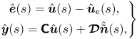 \begin{equation} \left.\begin{gathered} \hat{\boldsymbol{e}}(s) =\hat{\boldsymbol{u}}(s) - \hat{\boldsymbol{u}}_{e}(s),\\ \hat{\boldsymbol{y}}(s) = \boldsymbol{\mathsf{C}}\hat{\boldsymbol{u}}(s) + \boldsymbol{\mathcal{D}}\hat{\tilde{\boldsymbol{n}}}(s), \end{gathered}\right\} \end{equation}
where  $\hat {\boldsymbol {u}}(s)= ( s \boldsymbol{\mathsf{I}} - \boldsymbol{\mathsf{A}} )^{-1} \boldsymbol {\mathcal {B}}\hat {\tilde {\boldsymbol {f}}}(s)$ is the response generated by the stochastic forcing that is defined as $\boldsymbol {\mathcal {B}}\hat {\tilde {\boldsymbol {f}}}(s)$, and $\boldsymbol {\mathcal {D}}\hat {\tilde {\boldsymbol {n}}}(s)$ defines the sensor noise.
Now define the controller  $F(s)$ and transfer matrix $T_{\boldsymbol {ew}}(s)$, i.e.
 \begin{equation} \left.\begin{gathered} \hat{\boldsymbol{u}}_{e}(s) = F(s) \hat{\boldsymbol{y}}(s), \\ \hat{\boldsymbol{e}}(s) = T_{\boldsymbol{ew}}(s) \hat{\boldsymbol{w}}(s), \end{gathered}\right\} \end{equation}
where the explicit expression of  $T_{\boldsymbol {ew}}$ can be derived to be
 \begin{equation} T_{\boldsymbol{ew}}(s) = \left[ (\boldsymbol{\mathsf{I}}-F(s)\boldsymbol{\mathsf{C}})\left( s \boldsymbol{\mathsf{I}} - \boldsymbol{\boldsymbol{\mathsf{A}}} \right)^{{-}1}\boldsymbol{\mathcal{B}} ,\quad -F(s)\boldsymbol{\mathcal{D}} \right], \end{equation}
according to (D5). The goal of the  $H_2$ control problem includes finding a rational controller $F(s)$ that minimises the $H_2$ norm of the transfer matrix $T_{\boldsymbol {ew}}$ that links the external input $\boldsymbol {w}$ and the estimation error $\boldsymbol {e}$ (Zhou & Doyle Reference Zhou and Doyle1998), which directly builds up the foundation of the $H_2$-optimal estimation in Illingworth et al. (Reference Illingworth, Monty and Marusic2018). Details of the mechanism and methodology for solving the $H_2$ optimisation problem can be found in Doyle et al. (Reference Doyle, Glover, Khargonekar and Francis1989) or Zhou & Doyle (Reference Zhou and Doyle1998). The algorithm for solving the $H_2$-optimal problem has been integrated in MATLAB and can be solved via the function $\texttt {h2syn}$, i.e.
 \begin{equation} [F,T_{\boldsymbol{ew}},\gamma] = \texttt{h2syn}(G,n_{\boldsymbol{y}},n_{\boldsymbol{u_{e}}}), \end{equation}
where  $G$ is assigned in MATLAB via $G = \texttt {ss}(A,B,C,D)$, $n_{\boldsymbol {y}}$ and $n_{\boldsymbol {u_{e}}}$ are the dimensions of the measurement $\boldsymbol {y}$ and estimation $\boldsymbol {u}_{e}$, respectively, and $\gamma$ is the resultant minimum $H_2$ norm of $T_{\boldsymbol {ew}}$.
According to Doyle et al. (Reference Doyle, Glover, Khargonekar and Francis1989) and Zhou & Doyle (Reference Zhou and Doyle1998), the  $H_2$-optimal approach provides causal estimations, and utilises the measurement information at $\tau \leqslant t$ when estimating the flow state at time $t$. From the definition of the $H_2$ norm in (D1), the expected estimation error energy is minimised only when the forcing is white in time, i.e. the CSD tensors of the forcing at a given spatial scale $\boldsymbol {k}_{s}$ are unchanged for all the temporal frequencies.
D.1. The turbulent channel flow with $Re_\tau =934$

The distributions of the estimation errors at  $y^+ = 100$ with $Re_{\tau }=934$ in the TU case for different frequency bands are shown in figure 22. As in figure 22(a), the RBE-F results have the smallest estimation error at P1, since the RBE-F utilises the optimal transfer kernels for P1 to estimate the flow state at all the sequential frequency bands. From the second frequency band P2 on, the relative MSEs of the RBE-F results become larger than those from the GRBE. Meanwhile, the RBE-T results nearly overlap with the RBE-F results in almost all the considered frequency bands. On the other hand, the GRBE results in the TU and TR cases are pretty close to each other for the turbulence estimation.
Relative MSEs at  $y^+ = 100$ for different frequency bands of the turbulent channel flow with $Re_{\tau }=934$ in the TU case. ( $a$) The estimation error at separated frequency bands. ( $b$) The accumulated estimation error by sequentially increasing the considered numbers of frequency bands.
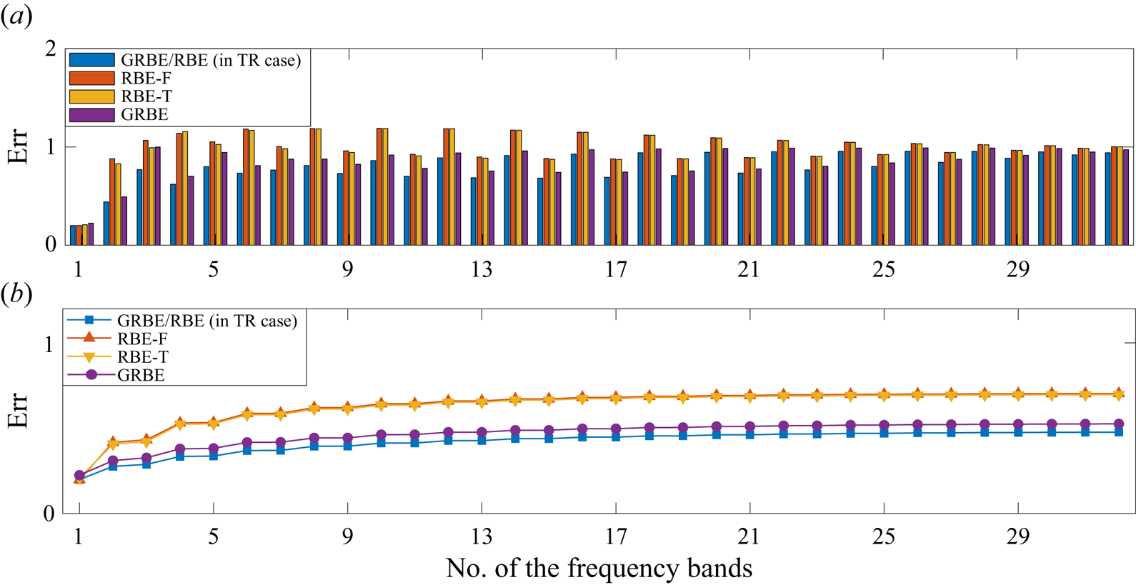
In figure 23, the instantaneous flow states at  $y^+ = 100$ within different frequency bands are depicted. For the first frequency band P1 with the lowest frequencies, all the tested methods provide reasonable results. For the sequential frequency bands P2 and P8, the patterns of the flow structures become different in the GRBE and RBE results. Although the estimated flow energies are lower than those from the DNS, the flow patterns of the GRBE results in the sequential frequency bands keep consistent with the DNS ones. Meanwhile, the flow patterns estimated by the RBE-F and RBE-T become different from the DNS results in the sequential frequency bands. Specifically, for P8 with higher frequencies, flow structures that are elongated in the spanwise direction can be observed in the RBE results, which are considered to contribute to the non-physical small-scale spanwise streaks in the RBE-T results shown in figure 6.
Instantaneous flow state at  $y^+ = 100$ in the TU case corresponding to the frequency bands of P1 (a,d,g,j), P2 (b,e,h,k) and P8 (c,f,i,l). The results are from DNS (a–c), GRBE (d–f), RBE-F (g–i) and RBE-T ( j–l).


 Open access