


1. Introduction
Recent advances in additive manufacturing, particularly in three-dimensional (3D) printing technologies, have revolutionized the design and fabrication of complex composite structures across various industries, including aerospace, biomedical engineering, and textiles. In the textile sector, 3D-printed fabrics and functional composites are increasingly being developed for their ability to integrate structural, aesthetic, and mechanical performance within a unified design process. These engineered textiles often feature periodic microstructures with stiff or rigid inclusions embedded in a softer matrix material, enabling tailored flexibility, durability, and deformation response. Understanding the mechanical behaviour of such thin composite structures under deformation requires a rigorous mathematical framework capable of capturing the interplay between microscale architecture and macroscopic geometry.
This work provides such a framework by analysing the simultaneous homogenization and dimension reduction (SHD) of thin plates reinforced with rigid inclusions in the non-linear elastic regime. The resulting limit models incorporate effective macroscopic strain constraints and non-linear coupling conditions, such as Monge–Ampère-type relations, which directly reflect the influence of the microstructural configuration on the global behaviour of the plate. These models are not only mathematically rigorous but also computationally efficient for simulating thin composite sheets in applications such as programmable textiles, morphing surfaces, and stretchable electronics, where microscale control is essential to achieving desirable macroscopic performance. By deriving effective plate theories from first principles, our analysis contributes to the design, optimization, and predictive modelling of next-generation textile composites fabricated through 3D printing technologies.
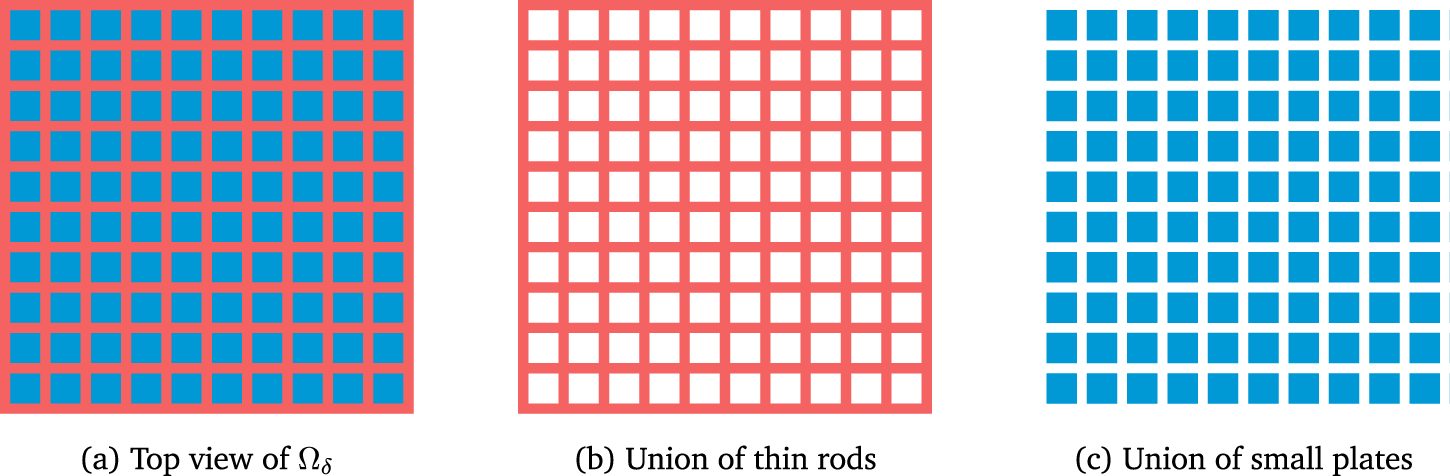
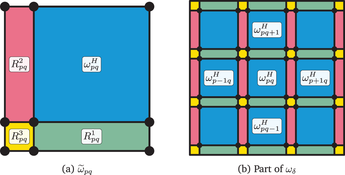
This paper presents a rigorous derivation of a limit model via SHD of thin plates reinforced with rigid substructures, within the framework of non-linear elasticity. The structure ( $\Omega_\delta$, a connected thin plate) under consideration consists of a soft plate formed by thin straight rods intersecting in two in-plane directions, creating a periodic structural frame ( $\Omega^S_{\varepsilon\delta}$, the connected soft part), with rigid inclusions ( $\Omega^H_{\varepsilon\delta}$, the disconnected hard part) filling the resulting holes; see Figure 1.
Blue and red indicate the hard and soft parts, respectively. (a) Top view of  $\Omega_\delta$. (b) Union of thin rods. (c) Union of small plates.

Figure 1 Long description
The image consists of three diagrams. The first diagram labeled 'a' shows the top view of Omega subscript delta, featuring a grid pattern with alternating squares. The second diagram labeled 'b' illustrates the union of thin rods, displaying a similar grid pattern with more prominent lines. The third diagram labeled 'c' depicts the union of small plates, showing a grid pattern with smaller squares. Each diagram represents different structural elements in a periodic arrangement.
There are two small parameters:  $\delta$, representing the plate thickness, and $\varepsilon$, denoting the periodicity. In this work, we consider the thin-plate regime characterized by $0 \lt 3\delta \lt \varepsilon$ and
 \begin{equation}
\lim_{(\varepsilon,\delta)\to(0,0)}\frac{\delta}{\varepsilon} = 0=\lim_{(\varepsilon,\delta)\to(0,0)}{\varepsilon^2\over \delta}.
\end{equation}
\begin{equation}
\lim_{(\varepsilon,\delta)\to(0,0)}\frac{\delta}{\varepsilon} = 0=\lim_{(\varepsilon,\delta)\to(0,0)}{\varepsilon^2\over \delta}.
\end{equation} The rigidity of the hard inclusions is enforced by requiring that the deformation gradient satisfies  $\nabla v \in \mathrm{SO}(3)$ in $\Omega^H_{\varepsilon\delta}$.
The aim of this paper is twofold. First, we establish a decomposition of deformations for thin plates with embedded rigid inclusions. Second, we utilize this decomposition, along with two rescaled unfolding operators and  $\Gamma$-convergence techniques, to derive a two-dimensional (2D) asymptotic model. Problems of this type are known as SHD problems. It is well known that the limiting behaviour of such composite structures depends sensitively on the scaling of the elastic energy; different energy regimes can lead to fundamentally different plate models that are not always consistent with one another, for a detailed description, see the seminal paper on hierarchy of thin plate models [Reference Friesecke, James and Müller18] via dimension reduction.
SHD constitute a highly active area of research. In the context of thin plates, the von Kármán regime has been studied in [Reference Griso, Orlik and Wackerle22, Reference Neukamm and Velčić25, Reference Velčić29], while the large-deformation regime has been examined in [Reference Cherdantsev and Cherednichenko7, Reference Falconi, Griso and Orlik17, Reference Hornung, Neukamm and Velčić23, Reference Velčić28]. In addition to the order of total energy, the limit models are also sensitive to the relative scaling of  $\delta$ and $\varepsilon$. The thin plate regime (when $\delta$ is of smaller order than $\varepsilon$, see (1.1) $_1$), was considered in [Reference Cherdantsev and Cherednichenko7, Reference Velčić28] in the large-deformation regime (higher than von Kármán) with similar restriction of (1.1) $_2$. To the best of our knowledge, in the context of SHD, the intermediate energy regime that lies between large deformation and von Kármán has not been explored. In this study, we focus on an intermediate energy regime for the total elastic energy (see Remark (4.13)).
The structure of the paper is as follows. General notations are introduced in Section 2. Section 3 provides the domain and problem description. In particular, the set of admissible deformations is defined by
 \begin{equation*}
\textbf{V}_{\varepsilon\delta} = \left\{v \in H^1(\Omega_\delta)^3\,\| \nabla v \in \mathrm{SO}(3)\ \text{in }\Omega^H_{\varepsilon\delta},\ v = I_d \text{on } \Gamma_\delta \right\},
\end{equation*}
\begin{equation*}
\textbf{V}_{\varepsilon\delta} = \left\{v \in H^1(\Omega_\delta)^3\,\| \nabla v \in \mathrm{SO}(3)\ \text{in }\Omega^H_{\varepsilon\delta},\ v = I_d \text{on } \Gamma_\delta \right\},
\end{equation*}where  $\Omega_\delta$ is the entire plate and $\Omega^H_{\varepsilon\delta}$ denotes the region containing the rigid substructures. The corresponding minimization problem is given by
 \begin{equation*}
\textbf{m}_{\varepsilon\delta} = \inf_{v \in \textbf{V}_{\varepsilon\delta}} \textbf{J}_{\varepsilon\delta}(v),
\end{equation*}
\begin{equation*}
\textbf{m}_{\varepsilon\delta} = \inf_{v \in \textbf{V}_{\varepsilon\delta}} \textbf{J}_{\varepsilon\delta}(v),
\end{equation*}where  $\textbf{J}_{\varepsilon\delta}$ is the total non-linear elastic energy. For general references on the theory of elasticity and plates, we refer the reader to [Reference Ciarlet11] and [Reference Ciarlet and Mardare12].
Section 4 contains the first aim of the paper, where we present the decomposition of deformation of thin plates reinforced with rigid inclusions. This section is divided into three subsections. In Subsection 4.1, we recall the decomposition of thin plate deformations from [Reference Blanchard and Griso2] and a short background in Remark 4.2; see also [Reference Blanchard and Griso1] for an introduction to the decomposition of rod deformations. In Subsection 4.2, using estimates from the previous subsection, we extend the decomposition to thin plates reinforced with rigid inclusions. Specifically, every 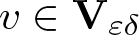 $v \in \textbf{V}_{\varepsilon\delta}$ can be decomposed as
 \begin{equation*}
v = V_e + \overline{v}, \quad \text{in } \Omega_\delta \ \text{with } \nabla v = \nabla V_e \in \mathrm{SO}(3) \text{in } \Omega^H_{\varepsilon\delta},
\end{equation*}
\begin{equation*}
v = V_e + \overline{v}, \quad \text{in } \Omega_\delta \ \text{with } \nabla v = \nabla V_e \in \mathrm{SO}(3) \text{in } \Omega^H_{\varepsilon\delta},
\end{equation*}where  $V_e$ is the elementary deformation and $\overline{v}$ is the residual deformation. In Subsection 4.3, we then use this decomposition along with the scaling of applied forces to obtain a bounded energy estimate for the minimization problem. More precisely, there exists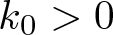 $k_0 \gt 0$ such that
 \begin{equation*}
-k_0 \leq \frac{\textbf{m}_{\varepsilon\delta}}{\varepsilon^2\delta^3} \leq 0.
\end{equation*}
\begin{equation*}
-k_0 \leq \frac{\textbf{m}_{\varepsilon\delta}}{\varepsilon^2\delta^3} \leq 0.
\end{equation*} The central goal of this paper is to characterize this rescaled minimization problem as both  $\varepsilon$ and $\delta$ tend to zero. Problems concerning SHD in both linear and non-linear elasticity are considered in [Reference Chakrabortty, Griso and Orlik4, Reference Falconi, Griso and Orlik17, Reference Griso, Khilkova, Orlik and Sivak19, Reference Griso, Khilkova, Orlik and Sivak20, Reference Griso, Orlik and Wackerle22, Reference Neukamm and Velčić25, Reference Velčić29] and the references therein. For background on homogenization and elasticity, we refer to [Reference Oleïnik, Shamaev and Yosifian26].
In Section 5, we recall and analyse two rescaled unfolding operators, which are adapted to the thin-plate setting. The standard periodic unfolding operator was first introduced in [Reference Cioranescu, Damlamian and Griso13] and further developed in [Reference Cioranescu, Damlamian and Griso14], while its rescaled counterpart, suited for SHD, is discussed in [Reference Griso, Orlik and Wackerle21] and [Reference Orlik, Falconi, Griso and Wackerle27]. These tools allow us to capture the multiscale behaviour of the deformation fields. Then, in Section 6, by combining the decomposition estimates from Section 4 with the properties of the rescaled unfolding operators, we characterize the asymptotic behaviour of the macroscopic and microscopic fields and rigorously derive the limit of the Green–St. Venant strain tensor.
Section 7 presents the main results and the second aim of the paper. In Subsections 7.1–7.2, we formulate the limiting unfolded minimization problem and prove the existence of a minimizer. The limiting macroscopic displacement  ${\mathcal{W}} = ({\mathcal{W}}_1, {\mathcal{W}}_2, {\mathcal{W}}_3) \in H^1({\omega})^2 \times H^2({\omega})$ satisfies the system:
 \begin{equation*}
e_{\alpha\beta}({\mathcal{W}}) + \frac{1}{2} \partial_\alpha {\mathcal{W}}_3 \partial_\beta {\mathcal{W}}_3 = 0,\quad \partial_{12} {\mathcal{W}}_3 = 0 \quad \text{in } {\omega}.
\end{equation*}
\begin{equation*}
e_{\alpha\beta}({\mathcal{W}}) + \frac{1}{2} \partial_\alpha {\mathcal{W}}_3 \partial_\beta {\mathcal{W}}_3 = 0,\quad \partial_{12} {\mathcal{W}}_3 = 0 \quad \text{in } {\omega}.
\end{equation*}These equations are equivalent to the homogeneous Monge–Ampère equation:
 \begin{equation*}
\det(\nabla^2_{x'} {\mathcal{W}}_3) = (\partial^2_{11} {\mathcal{W}}_3)(\partial^2_{22} {\mathcal{W}}_3) - (\partial^2_{12} {\mathcal{W}}_3)^2 = 0, \quad \text{in } {\omega},
\end{equation*}
\begin{equation*}
\det(\nabla^2_{x'} {\mathcal{W}}_3) = (\partial^2_{11} {\mathcal{W}}_3)(\partial^2_{22} {\mathcal{W}}_3) - (\partial^2_{12} {\mathcal{W}}_3)^2 = 0, \quad \text{in } {\omega},
\end{equation*}with the additional constraint 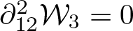 $\partial^2_{12} {\mathcal{W}}_3 = 0$ in ${\omega}$. As a consequence, we show that there exist functions ${\mathcal{W}}_3^{(1)}$ and ${\mathcal{W}}_3^{(2)}$ such that
 \begin{equation*}
\left\{
\begin{aligned}
{\mathcal{W}}_3(x_1, x_2) &= {\mathcal{W}}_3^{(2)}(x_1) + {\mathcal{W}}_3^{(1)}(x_2), \quad {\mathcal{W}}_3^{(1)}(x_2)\, {\mathcal{W}}_3^{(2)}(x_1) = 0, \\
{\mathcal{W}}_1(x_1, x_2) &= {\mathcal{W}}_1(x_1) = -\frac{1}{2} \int_0^{x_1} |d_1 {\mathcal{W}}_3^{(2)}(t)|^2 \, dt, \\
{\mathcal{W}}_2(x_1, x_2) &= {\mathcal{W}}_2(x_2) = -\frac{1}{2} \int_0^{x_2} |d_2 {\mathcal{W}}_3^{(1)}(t)|^2 \, dt,
\end{aligned}
\right.
\quad \text{for } (x_1, x_2) \in {\omega}.
\end{equation*}
\begin{equation*}
\left\{
\begin{aligned}
{\mathcal{W}}_3(x_1, x_2) &= {\mathcal{W}}_3^{(2)}(x_1) + {\mathcal{W}}_3^{(1)}(x_2), \quad {\mathcal{W}}_3^{(1)}(x_2)\, {\mathcal{W}}_3^{(2)}(x_1) = 0, \\
{\mathcal{W}}_1(x_1, x_2) &= {\mathcal{W}}_1(x_1) = -\frac{1}{2} \int_0^{x_1} |d_1 {\mathcal{W}}_3^{(2)}(t)|^2 \, dt, \\
{\mathcal{W}}_2(x_1, x_2) &= {\mathcal{W}}_2(x_2) = -\frac{1}{2} \int_0^{x_2} |d_2 {\mathcal{W}}_3^{(1)}(t)|^2 \, dt,
\end{aligned}
\right.
\quad \text{for } (x_1, x_2) \in {\omega}.
\end{equation*} The resulting limit model is of constrained Kármán type. Such constrained Kármán plate theories arise in the hierarchy of limit models for homogeneous thin plates, as derived in the seminal work [Reference Friesecke, James and Müller18]. In the present work, we extend this framework to heterogeneous thin plates with rigid reinforcements. Homogenization for elastic bodies with rigid inclusions (without a dimension-reduction parameter  $\delta$) has been studied in [Reference Christowiak and Kreisbeck10, Reference Düll, Engl and Kreisbeck15, Reference Engl, Kreisbeck and Ritorto16]. For a related rigidly reinforced thin plate $\Omega_\delta$ in the linearized setting, the derivation of an effective model in the von Kármán regime via a Kirchhoff–Love displacement decomposition is considered in [Reference Chakrabortty, Griso and Orlik5]. In contrast, homogenization of high-contrast elastic composites with soft inclusions in non-linear elasticity is addressed in [Reference Cherdantsev and Cherednichenko6, Reference Cherdantsev, Cherednichenko and Neukamm8]; see [Reference Chakrabortty, Griso and Orlik4, Reference Cherednichenko and Evans9] for corresponding dimension-reduction results in high-contrast settings.
The homogenized problem and the construction of a recovery sequence (or test deformations) are detailed in Subsections 7.3–7.4. Using a form of  $\Gamma$-convergence, we then establish our main result:
 \begin{equation*}
\lim_{(\varepsilon,\delta)\to(0,0)} \frac{\textbf{m}_{\varepsilon\delta}}{\varepsilon^2\delta^3} = \textbf{m}=\textbf{J}_{hom}({\cal W}_3),
\end{equation*}
\begin{equation*}
\lim_{(\varepsilon,\delta)\to(0,0)} \frac{\textbf{m}_{\varepsilon\delta}}{\varepsilon^2\delta^3} = \textbf{m}=\textbf{J}_{hom}({\cal W}_3),
\end{equation*}where  $\textbf{J}_{hom}$ is the homogenized energy and ${\mathcal{W}}_3$ is the limit macroscopic bending displacements.
Interestingly, in the limit, we obtain two functionals  $\textbf{J}_{hom}^{(1)}$ and $\textbf{J}_{hom}^{(2)}$ whose respective minima are $\textbf{m}^{(1)}$ and $\textbf{m}^{(2)}$, and we find
 \begin{equation*}
\textbf{m} = \min\left\{\textbf{m}^{(1)},\, \textbf{m}^{(2)}\right\},\quad \textbf{m}^{({\alpha})}=\textbf{J}_{hom}^{({\alpha})}({\mathcal{W}}^{({\alpha})}_3).
\end{equation*}
\begin{equation*}
\textbf{m} = \min\left\{\textbf{m}^{(1)},\, \textbf{m}^{(2)}\right\},\quad \textbf{m}^{({\alpha})}=\textbf{J}_{hom}^{({\alpha})}({\mathcal{W}}^{({\alpha})}_3).
\end{equation*} In particular, if  $\textbf{m}^{(1)} = \textbf{m}^{(2)}$, then the limit problem admits at least two distinct stable minimizers. These minimizers can be described in a simple and explicit form, using the cell problems.
For a general introduction to  $\Gamma$-convergence, we refer the reader to [Reference Maso24] and [Reference Braides3].
Finally, Appendix A provides the proofs of technical estimates needed to establish the existence of a minimizer for the limiting energy functional.
2. Notations
The following notation will be used:
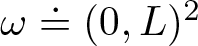
• ${\omega}\doteq(0,L)^2$,
$\gamma\doteq\{0\}\times (0,l)\cup (0,l)\times \{0\}$ with
$0 \lt l \lt L$,
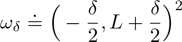
${\omega}_\delta\doteq\displaystyle\Big(-{\delta\over 2},L+{\delta\over 2}\Big)^2$.
${\omega}\doteq(0,L)^2$,
$\gamma\doteq\{0\}\times (0,l)\cup (0,l)\times \{0\}$ with
$0 \lt l \lt L$,
${\omega}_\delta\doteq\displaystyle\Big(-{\delta\over 2},L+{\delta\over 2}\Big)^2$.•
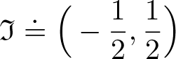
$\displaystyle {\mathfrak{I}}\doteq \Big(-{1\over 2},{1\over 2}\Big)$,
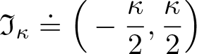
$\displaystyle {\mathfrak{I}}_\kappa\doteq \Big(-{\kappa\over 2},{\kappa\over 2}\Big)$,
$\kappa \gt 0$.• We choose
$\varepsilon$ such that
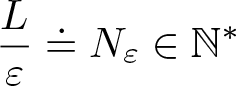
$\displaystyle {L\over \varepsilon}\doteq N_\varepsilon\in {\mathbb{N}}^*$,
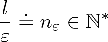
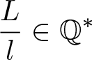
$\displaystyle {l\over \varepsilon}\doteq n_\varepsilon\in {\mathbb{N}}^*$ (This implies that
$\displaystyle {L\over l}\in \mathbb{Q}^*$.).•
${\mathcal K}_\varepsilon\doteq \{0,\ldots,N_\varepsilon\}^2$,
${\mathcal K}^*_\varepsilon\doteq \{0,\ldots,N_\varepsilon-1\}^2$,
$\overline{{\mathcal K}}_\varepsilon\doteq \{-1,\ldots,N_\varepsilon\}^2$,
${\mathcal K}_\varepsilon^{(1)}\doteq\{0,\ldots,N_\varepsilon-1\}\times \{0,\ldots,N_\varepsilon\}$,
${\mathcal K}_\varepsilon^{(2)}\doteq\{0,\ldots,N_\varepsilon\}\times \{0,\ldots,N_\varepsilon-1\}$.• For any
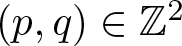
$(p,q)\in {\mathbb{Z}}^2$,
\begin{equation*}
\left\{\begin{aligned}
& {\omega}_{pq}\doteq (p\varepsilon,p\varepsilon+\varepsilon)\times (q\varepsilon,q\varepsilon+\varepsilon),\qquad \Omega_{pq}\doteq {\omega}_{pq}\doteq \times {\mathfrak{I}}_\delta,\\
& \widetilde {{\omega}}_{pq}\doteq \Big(p\varepsilon-{\delta\over 2},(p+1)\varepsilon+{\delta\over 2}\Big)\times \Big(q\varepsilon-{\delta\over 2},(q+1)\varepsilon+{\delta\over 2}\Big),\quad \widetilde {\Omega}_{pq}\doteq \widetilde {{\omega}}_{pq}\times {\mathfrak{I}}_\delta, \\
& {\omega}^H_{pq}\doteq \Big(p\varepsilon+{\delta\over 2},(p+1)\varepsilon-{\delta\over 2}\Big)\times \Big(q\varepsilon+{\delta\over 2},(q+1)\varepsilon-{\delta\over 2}\Big),\quad \Omega^H_{pq}\doteq{\omega}^H_{pq}\times {\mathfrak{I}}_\delta,\\
& {\omega}^H_{{\varepsilon\delta}}=\bigcup_{(p,q)\in{\mathcal K}_\varepsilon^*}{\omega}^H_{pq}, \quad {\omega}^S_{{\varepsilon\delta}}\doteq {\omega}_\delta \setminus \overline{{\omega}^H_{{\varepsilon\delta}}},\quad \Omega_{\delta}\doteq {\omega}_\delta\times {\mathfrak{I}}_\delta,\quad \Omega^S_{\varepsilon\delta}=\Omega_{\delta}\setminus \overline{\Omega^H_{{\varepsilon\delta}}}={\omega}^S_{\varepsilon\delta} \times {\mathfrak{I}}_\delta.
\end{aligned}
\right.
\end{equation*}•
$\textbf{M}_3$ is the space of
$3\times 3$ real matrices,
${\textbf{S}}_3$ the space of real
$3\times 3$ symmetric matrices,
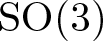
$\mathrm{SO}(3)$ the space of special orthogonal matrices,
$\textbf{I}_3$ the identity matrix of
$\textbf{M}_3$.•
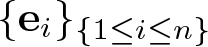
$\{\textbf{e}_i\}_{\{1\leq i\leq n\}}$ the standard basis of
${\mathbb{R}}^n$,
$I_d$ is the identity mapping of
${\mathbb{R}}^n$,
$n\geq 1$.•
$|\cdot|$ the standard Euclidean norm in
${\mathbb{R}}^n$,
$n\geq 1$, and Frobenius norm in
$\textbf{M}_3$.•
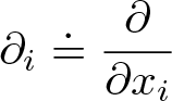
$\displaystyle \partial_i\doteq\frac{\partial}{\partial x_i}$,
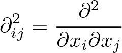
$\displaystyle{\partial}^2_{ij}={{\partial}^2\over {\partial} x_i{\partial} x_j}$ for
$i,j\in \{1,2,3\}$, and
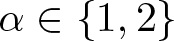
$\displaystyle d_\alpha={d\over dx_\alpha},\quad d^2_\alpha={d^2\over dx_\alpha^2},\quad \alpha\in\{1,2\}$.•
$Y_1=(0,1)\times \displaystyle {\mathfrak{I}}$,
$Y_2=\displaystyle {\mathfrak{I}}\times (0,1)$, and
${\mathcal{Y}}_\alpha=Y_\alpha\times \displaystyle {\mathfrak{I}}$,
$\alpha\in\{1,2\}$.•
$x'=(x_1,x_2)$ the current point in
${\mathbb{R}}^2$ and
$x=(x_1,x_2,x_3)$ the current point in
${\mathbb{R}}^3$,• For any
$u\in H^1(\Omega_\delta)^3$ the linearized strain tensor
$e(u)$ is the
$3\times 3$ symmetric matrix whose entries are
\begin{equation*}
e_{ij}(u)={1\over 2}\big({\partial}_i u_j+{\partial}_j u_i\big),\qquad \forall (i,j)\in \{1,2,3\}^2.
\end{equation*}For any
$\phi=\phi_1\textbf{e}_1+\phi_2\textbf{e}_2\in H^1({\omega}_\delta)^3$
(2.1)and for\begin{equation}
e_{\alpha\beta}(\phi)={1\over 2}(\partial_\alpha \phi_\beta+\partial_\beta \phi_\alpha),\qquad (\alpha,\beta)\in\{1,2\}^2,
\end{equation}
$v\in H^1({\cal Y}_{\alpha})^3$, we have
\begin{equation*}
e_{ij,y}(v)={1\over 2}\big({\partial}_{y_i} v_j+{\partial}_{y_j} v_i\big),\quad\text{with}\quad \partial_{y_i}\doteq\frac{\partial}{\partial y_i},\quad \forall (i,j)\in \{1,2,3\}^2.
\end{equation*}• If (p.q) labels a system of equations, we write (p.q)
$_i$ for its (
$i$)th component; likewise, (p.q)
$_{i,j}$ denotes components (
$i$) and (
$j$).
































Throughout this paper, we choose the parameters  $0 \lt {3}\delta \lt \varepsilon\ll1$ satisfying
 \begin{equation}
\lim_{(\varepsilon,\delta)\to(0,0)}{\delta\over \varepsilon}=0=\lim_{(\varepsilon,\delta)\to(0,0)}{\varepsilon^2\over \delta}.
\end{equation}
\begin{equation}
\lim_{(\varepsilon,\delta)\to(0,0)}{\delta\over \varepsilon}=0=\lim_{(\varepsilon,\delta)\to(0,0)}{\varepsilon^2\over \delta}.
\end{equation}  $C$ denotes a generic constant independent of $\varepsilon$ and $\delta$. By convention in all the estimates, we simply write $L^2(\cdot)$ instead of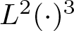 $L^2(\cdot)^3$ or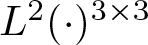 $L^2(\cdot)^{3\times 3}$, we write the complete spaces when we give weak or strong convergence. The Greek letters $\alpha,\, \beta$ belong to $\{1,2\}$ and the Latin letters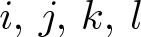 $i,\,j,\,k,\,l$ to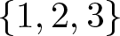 $ \{1,2,3\}$ (if not specified). We use the Einstein convention of summation over repeated indices.
3. Problem setting
The rigid reinforced composite plate, in its stress-free reference configuration, occupies the region
 \begin{equation*}\Omega_{\delta}={\omega}_\delta\times {\mathfrak{I}}_\delta=\hbox{Interior}\big(\overline{\Omega^S_{\varepsilon\delta}}\cup\overline{\Omega^H_{{\varepsilon\delta}}}\big).\end{equation*}
 We define the families of beams oriented along  $\textbf{e}_1$ and $\textbf{e}_2$ by
 \begin{equation*}
\begin{aligned}
&\Omega^{(1)}_{\varepsilon\delta}\doteq {\omega}^{(1)}_{\varepsilon\delta}\times {\mathfrak{I}}_\delta,\quad {\omega}^{(1)}_{\varepsilon\delta}\doteq\bigcup_{q=0}^{N_\varepsilon}\Big(-{\delta\over 2},L+{\delta\over 2}\Big)\times \Big(q\varepsilon-{\delta\over 2},q\varepsilon+{\delta\over 2}\Big),\\
& \Omega^{(2)}_{\varepsilon\delta}\doteq {\omega}^{(2)}_{\varepsilon\delta}\times {\mathfrak{I}}_\delta,\quad {\omega}^{(2)}_{\varepsilon\delta}\doteq\bigcup_{p=0}^{N_\varepsilon}\Big(p\varepsilon-{\delta\over 2},p\varepsilon+{\delta\over 2}\Big)\times \Big(-{\delta\over 2},L+{\delta\over 2}\Big),\\
&\quad \hbox{so}\quad \Omega^S_{\varepsilon\delta}=\Omega^{(1)}_{\varepsilon\delta}\cup \Omega^{(2)}_{\varepsilon\delta}.
\end{aligned}
\end{equation*}
\begin{equation*}
\begin{aligned}
&\Omega^{(1)}_{\varepsilon\delta}\doteq {\omega}^{(1)}_{\varepsilon\delta}\times {\mathfrak{I}}_\delta,\quad {\omega}^{(1)}_{\varepsilon\delta}\doteq\bigcup_{q=0}^{N_\varepsilon}\Big(-{\delta\over 2},L+{\delta\over 2}\Big)\times \Big(q\varepsilon-{\delta\over 2},q\varepsilon+{\delta\over 2}\Big),\\
& \Omega^{(2)}_{\varepsilon\delta}\doteq {\omega}^{(2)}_{\varepsilon\delta}\times {\mathfrak{I}}_\delta,\quad {\omega}^{(2)}_{\varepsilon\delta}\doteq\bigcup_{p=0}^{N_\varepsilon}\Big(p\varepsilon-{\delta\over 2},p\varepsilon+{\delta\over 2}\Big)\times \Big(-{\delta\over 2},L+{\delta\over 2}\Big),\\
&\quad \hbox{so}\quad \Omega^S_{\varepsilon\delta}=\Omega^{(1)}_{\varepsilon\delta}\cup \Omega^{(2)}_{\varepsilon\delta}.
\end{aligned}
\end{equation*}On a portion of the boundary of the soft part, we impose the homogeneous boundary condition
 \begin{equation}
v=I_d,\quad\text{a.e. on }\Gamma_\delta=\Big[{\mathfrak{I}}_\delta\times \Big(-{\delta\over 2},l+{\delta\over 2}\Big)\cup \Big(-{\delta\over 2},l+{\delta\over 2}\Big)\times {\mathfrak{I}}_\delta\Big]\times {\mathfrak{I}}_\delta.
\end{equation}
\begin{equation}
v=I_d,\quad\text{a.e. on }\Gamma_\delta=\Big[{\mathfrak{I}}_\delta\times \Big(-{\delta\over 2},l+{\delta\over 2}\Big)\cup \Big(-{\delta\over 2},l+{\delta\over 2}\Big)\times {\mathfrak{I}}_\delta\Big]\times {\mathfrak{I}}_\delta.
\end{equation} We assume that the deformation is rigid in the subdomains  $\Omega^H_{pq}$ for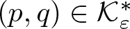 $(p,q)\in{\mathcal{K}}_\varepsilon^*$, namely,
 \begin{equation*}\nabla v\in\mathrm{SO}(3),\quad\text{a.e. in}\ \Omega^H_{\varepsilon\delta}.\end{equation*}
Hence,
 \begin{equation}
\begin{aligned}
&v(x)=\textbf{a}_{pq}+\textbf{R}_{pq}\overline{x}_{pq}\ \ \text{a.e. in } \Omega^H_{pq},\quad (\textbf{a}_{pq},\textbf{R}_{pq})\in{\mathbb{R}}^3\times \mathrm{SO}(3),\quad \forall (p,q)\in{\mathcal{K}}_\varepsilon^*,\\
& \overline{x}_{pq}=x-p\varepsilon\textbf{e}_1-q\varepsilon\textbf{e}_2,\qquad \overline{x}^{'}_{pq}=\overline{x}_{pq}-x_3\textbf{e}_3.
\end{aligned}
\end{equation}
\begin{equation}
\begin{aligned}
&v(x)=\textbf{a}_{pq}+\textbf{R}_{pq}\overline{x}_{pq}\ \ \text{a.e. in } \Omega^H_{pq},\quad (\textbf{a}_{pq},\textbf{R}_{pq})\in{\mathbb{R}}^3\times \mathrm{SO}(3),\quad \forall (p,q)\in{\mathcal{K}}_\varepsilon^*,\\
& \overline{x}_{pq}=x-p\varepsilon\textbf{e}_1-q\varepsilon\textbf{e}_2,\qquad \overline{x}^{'}_{pq}=\overline{x}_{pq}-x_3\textbf{e}_3.
\end{aligned}
\end{equation}Since the soft part is glued to the hard part, the deformation and the associated response are continuous across the interface. Finally, the set of admissible deformations is
 \begin{equation*}
\begin{aligned}
\textbf{V}_{\varepsilon\delta}\doteq \big\{v\in H^1(\Omega_{\delta})^3\;|\; \text{such that}\ v\ \text{satisfies (3.1)--(3.2)}\big\}.
\end{aligned}
\end{equation*}
\begin{equation*}
\begin{aligned}
\textbf{V}_{\varepsilon\delta}\doteq \big\{v\in H^1(\Omega_{\delta})^3\;|\; \text{such that}\ v\ \text{satisfies (3.1)--(3.2)}\big\}.
\end{aligned}
\end{equation*} Let  $\textbf{W}_{\varepsilon\delta}$ denote the elastic energy density of the material. The total elastic energy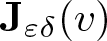 $\textbf{J}_{\varepsilon\delta}(v)$ over $\textbf{V}_{\varepsilon\delta}$ is given by
 \begin{equation*}
\textbf{J}_{\varepsilon\delta}(v)=\int_{\Omega^S_{\varepsilon\delta}}\textbf{W}_{\varepsilon\delta}(x,\nabla v)\,dx- \int_{\Omega_{\delta}}f_{\varepsilon\delta}\cdot(v-I_d)\,dx,
\end{equation*}
\begin{equation*}
\textbf{J}_{\varepsilon\delta}(v)=\int_{\Omega^S_{\varepsilon\delta}}\textbf{W}_{\varepsilon\delta}(x,\nabla v)\,dx- \int_{\Omega_{\delta}}f_{\varepsilon\delta}\cdot(v-I_d)\,dx,
\end{equation*}where the local energy density  $\textbf{W}_{\varepsilon\delta}\, :\ \, \Omega^S_{\varepsilon\delta} \times \textbf{M}_3 \longrightarrow {\mathbb{R}}^+\cup\{+\infty\}$ is defined by
 \begin{equation}
\textbf{W}_{\varepsilon\delta}(x , F)=
\left\{\begin{aligned}
& \textbf{Q}_{\varepsilon\delta}\big(x , \textbf{E}(F)\big) &&\hbox{if}\;\; \hbox{det}(F) \gt 0,\\
& +\infty &&\hbox{if}\;\; \hbox{det}(F)\leq 0,
\end{aligned}
\right. \quad\hbox{for a.e. } x \in \Omega^S_{\varepsilon\delta},
\end{equation}
\begin{equation}
\textbf{W}_{\varepsilon\delta}(x , F)=
\left\{\begin{aligned}
& \textbf{Q}_{\varepsilon\delta}\big(x , \textbf{E}(F)\big) &&\hbox{if}\;\; \hbox{det}(F) \gt 0,\\
& +\infty &&\hbox{if}\;\; \hbox{det}(F)\leq 0,
\end{aligned}
\right. \quad\hbox{for a.e. } x \in \Omega^S_{\varepsilon\delta},
\end{equation}where, for every 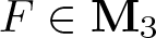 $F\in \textbf{M}_3$, we set
 \begin{equation*}
\textbf{E}(F)={1\over 2}\big(F^TF-\textbf{I}_3\big).
\end{equation*}
\begin{equation*}
\textbf{E}(F)={1\over 2}\big(F^TF-\textbf{I}_3\big).
\end{equation*} Since 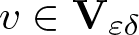 $v\in\textbf{V}_{\varepsilon\delta}$, equality (3.2) implies
 \begin{equation}
\textbf{D}(v)\doteq\|\mathrm{dist}(\nabla v, \mathrm{SO}(3))\|_{L^2(\Omega_\delta)}=\|\mathrm{dist}(\nabla v, \mathrm{SO}(3))\|_{L^2(\Omega^S_{\varepsilon\delta})},
\end{equation}
\begin{equation}
\textbf{D}(v)\doteq\|\mathrm{dist}(\nabla v, \mathrm{SO}(3))\|_{L^2(\Omega_\delta)}=\|\mathrm{dist}(\nabla v, \mathrm{SO}(3))\|_{L^2(\Omega^S_{\varepsilon\delta})},
\end{equation}that is, the contribution of the stiff part to the total energy is zero.
The quadratic form  $\textbf{Q}_{\varepsilon\delta}$ is defined (in Voigt matrix representation) by
 \begin{equation}
\textbf{Q}_{\varepsilon\delta}(x,S)=\textbf{S}^T{\mathbb{A}}_{{\varepsilon\delta}}(x)\textbf{S}=\langle {\mathbb{A}}_{\varepsilon\delta}\textbf{S},\textbf{S}\rangle,\quad\forall\, S\in{\mathbb{R}}^6,
\end{equation}
\begin{equation}
\textbf{Q}_{\varepsilon\delta}(x,S)=\textbf{S}^T{\mathbb{A}}_{{\varepsilon\delta}}(x)\textbf{S}=\langle {\mathbb{A}}_{\varepsilon\delta}\textbf{S},\textbf{S}\rangle,\quad\forall\, S\in{\mathbb{R}}^6,
\end{equation}where
 \begin{equation*}\textbf{S}=\left(\begin{matrix}
S_{11}&S_{22}&S_{33}&2S_{23}& 2S_{13}& 2 S_{12}
\end{matrix}\right)^T,\quad\forall\,S=[S_{ij}]\in\textbf{S}_3.\end{equation*}
\begin{equation*}\textbf{S}=\left(\begin{matrix}
S_{11}&S_{22}&S_{33}&2S_{23}& 2S_{13}& 2 S_{12}
\end{matrix}\right)^T,\quad\forall\,S=[S_{ij}]\in\textbf{S}_3.\end{equation*} It is assumed that the Hooke coefficient  ${\mathbb{A}}_{{\varepsilon\delta}}\in L^\infty(\Omega_{\varepsilon\delta}^S)^{6\times 6}$ is symmetric (A classical example of a material satisfying the above assumptions is the St. Venant–Kirchhoff material [see [Reference Ciarlet11] for more details].), positive definite, and satisfies, for some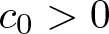 $c_0 \gt 0$,
 \begin{equation}
\langle {\mathbb{A}}_{{\varepsilon\delta}}\textbf{S},\textbf{S}\rangle\geq c_0|\textbf{S}|^2,\quad\forall\,\textbf{S}\in{\mathbb{R}}^6.
\end{equation}
\begin{equation}
\langle {\mathbb{A}}_{{\varepsilon\delta}}\textbf{S},\textbf{S}\rangle\geq c_0|\textbf{S}|^2,\quad\forall\,\textbf{S}\in{\mathbb{R}}^6.
\end{equation} The applied forces are prescribed as follows: let 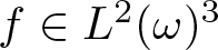 $f\in L^2({\omega})^3$, and define $f_{\varepsilon\delta}\in L^2(\Omega_\delta)^3$ by rescaling $f$ according to
 \begin{equation*}
f_{\varepsilon\delta}(x)=\sum_{\alpha=1}^2{\varepsilon\delta} f_\alpha(x')\textbf{e}_{\alpha}+({\varepsilon\delta})^{3/2} f_3(x')\textbf{e}_3,\quad \text{a.e. in}\ \Omega_\delta.
\end{equation*}
\begin{equation*}
f_{\varepsilon\delta}(x)=\sum_{\alpha=1}^2{\varepsilon\delta} f_\alpha(x')\textbf{e}_{\alpha}+({\varepsilon\delta})^{3/2} f_3(x')\textbf{e}_3,\quad \text{a.e. in}\ \Omega_\delta.
\end{equation*} Finally, for the given applied force  $f_{{\varepsilon\delta}}$, the non-linear elasticity problem reads (in the energy minimization formulation)
 \begin{equation}
\left\{
\begin{aligned}
&\hbox{Find}\ \textbf{m}_{\varepsilon\delta}\ \text{such that}\\
& \textbf{m}_{\varepsilon\delta}=\inf_{v\in\textbf{V}_{\varepsilon\delta}}\textbf{J}_{\varepsilon\delta}(v).
\end{aligned}
\right.
\end{equation}
\begin{equation}
\left\{
\begin{aligned}
&\hbox{Find}\ \textbf{m}_{\varepsilon\delta}\ \text{such that}\\
& \textbf{m}_{\varepsilon\delta}=\inf_{v\in\textbf{V}_{\varepsilon\delta}}\textbf{J}_{\varepsilon\delta}(v).
\end{aligned}
\right.
\end{equation}It should be noted that the existence of a minimizer for this problem is still open.
4. Estimates for the deformations in
$\textbf{V}_{\varepsilon\delta}$

In this section, we investigate the structure of admissible deformations for thin plates reinforced by rigid inclusions. We start by recalling the classical decomposition results for thin plates from [Reference Blanchard and Griso2] and their main properties. Building on these results, we derive several global estimates that will be needed in subsequent constructions. The main outcome of this section is an extension of the decomposition to the composite setting, where the presence of rigid substructures imposes additional geometric constraints. This decomposition is a key ingredient for establishing uniform energy bounds and for analysing the asymptotic behaviour of the deformation fields. Finally, we conclude the section by proving the existence of a minimizing sequence for the problem (3.7).
4.1. Recall of the decomposition of plate deformations
Theorem 4.1. (Theorem 3.4 in [Reference Blanchard and Griso2])
There exists a constant  $C$ (depending only on $L$) such that, for any deformation $v$ in $\mathbf{V}_{\varepsilon\delta}$ satisfying
 \begin{equation}
\mathbf{D}(v)\leq C\delta^{3/2}
\end{equation}
\begin{equation}
\mathbf{D}(v)\leq C\delta^{3/2}
\end{equation}we have the decomposition
 \begin{equation}
v=\mathfrak{V}+x_3\mathfrak{R}\textbf{e}_3+\overline{\mathfrak{v}}
\end{equation}
\begin{equation}
v=\mathfrak{V}+x_3\mathfrak{R}\textbf{e}_3+\overline{\mathfrak{v}}
\end{equation}where
 \begin{equation}
\mathfrak{V} \in H^1({\omega}_\delta)^3,\qquad \mathfrak{R} \in H^1\big({\omega}_\delta; \mathrm{SO}(3)\big),\qquad \overline{\mathfrak{v}}\in H^1(\Omega_\delta)^3.
\end{equation}
\begin{equation}
\mathfrak{V} \in H^1({\omega}_\delta)^3,\qquad \mathfrak{R} \in H^1\big({\omega}_\delta; \mathrm{SO}(3)\big),\qquad \overline{\mathfrak{v}}\in H^1(\Omega_\delta)^3.
\end{equation}These fields satisfy
 \begin{equation}
\mathfrak{V}+x_3\mathfrak{R}\textbf{e}_3=I_d,\quad\overline{\mathfrak{v}}=0\quad \hbox{a.e. on }\Gamma_\delta,\quad \int_{{\mathfrak{I}}_\delta}\overline{\mathfrak{v}}\,dx_3=0,\quad\text{a.e. in}\ {\omega}_\delta.
\end{equation}
\begin{equation}
\mathfrak{V}+x_3\mathfrak{R}\textbf{e}_3=I_d,\quad\overline{\mathfrak{v}}=0\quad \hbox{a.e. on }\Gamma_\delta,\quad \int_{{\mathfrak{I}}_\delta}\overline{\mathfrak{v}}\,dx_3=0,\quad\text{a.e. in}\ {\omega}_\delta.
\end{equation}We also have the following estimates (see (3.4)):
 \begin{equation}
\begin{aligned}
&\|\overline{\mathfrak{v}}\|_{L^2(\Omega_\delta)}+\delta\|\nabla\overline{\mathfrak{v}}\|_{L^2(\Omega_\delta)}\le C\delta \mathbf{D}(v),\\
&\delta\bigl\|\partial_{\alpha} \mathfrak{R}\big\|_{L^2(\omega_\delta)}+ \bigl\|\partial_{\alpha} \mathfrak{V}-\mathfrak{R} \textbf{e}_\alpha\big\|_{L^2(\omega_\delta)}\le {C\over \delta^{1/2}}\mathbf{D}(v),\\
& \bigl\|\nabla v-\mathfrak{R} \big\|_{L^2(\Omega_\delta)}\le C\mathbf{D}(v).
\end{aligned}
\end{equation}
\begin{equation}
\begin{aligned}
&\|\overline{\mathfrak{v}}\|_{L^2(\Omega_\delta)}+\delta\|\nabla\overline{\mathfrak{v}}\|_{L^2(\Omega_\delta)}\le C\delta \mathbf{D}(v),\\
&\delta\bigl\|\partial_{\alpha} \mathfrak{R}\big\|_{L^2(\omega_\delta)}+ \bigl\|\partial_{\alpha} \mathfrak{V}-\mathfrak{R} \textbf{e}_\alpha\big\|_{L^2(\omega_\delta)}\le {C\over \delta^{1/2}}\mathbf{D}(v),\\
& \bigl\|\nabla v-\mathfrak{R} \big\|_{L^2(\Omega_\delta)}\le C\mathbf{D}(v).
\end{aligned}
\end{equation} Here, the constants are independent of  $\delta$ and $L$.
$L$.
Let 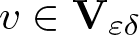 $v\in \textbf{V}_{\varepsilon\delta}$ be such that it satisfies (3.2) and (4.1). By the previous theorem, $v$ admits a decomposition of the form (4.2) satisfying (4.4). We recall (see [Reference Blanchard and Griso2, Theorem 3.3]) that
 \begin{equation*}\mathfrak{V}(x')={1\over 2\delta}\int_{-\delta}^\delta v(x',x_3)dx_3\qquad \hbox{for a.e. } x'\in {\omega}_\delta.\end{equation*}
 As a consequence, for all 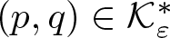 $(p,q)\in{\mathcal K}_\varepsilon^\ast$, using (3.2) we obtain
 \begin{equation}
\mathfrak{V}(x')=\textbf{a}_{pq}+\textbf{R}_{pq}\overline{x}^{'}_{pq},\quad \text{a.e. in}\ {\omega}^H_{pq}.
\end{equation}
\begin{equation}
\mathfrak{V}(x')=\textbf{a}_{pq}+\textbf{R}_{pq}\overline{x}^{'}_{pq},\quad \text{a.e. in}\ {\omega}^H_{pq}.
\end{equation}Remark 4.2. The decomposition (4.2) states that under the assumption (4.1) (see (6.1)), one can extract an approximate rigid motion at each in-plane point 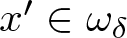 $x'\in{\omega}_\delta$. The decomposition has two components, one the elementary (rigid-fibre) part $\mathfrak{V}+x_3\mathfrak{R}\textbf{e}_3$ and the warping $\overline{\mathfrak{v}}$. The field $\mathfrak{V}$ represents the midsurface deformation (a thickness-averaged translation). The field $\mathfrak{R}$ is a rotation field describing the local orientation of the thickness fibres. The remainder $\overline{\mathfrak{v}}$ is a normalized non-rigid correction capturing the genuinely 3D part of the deformation. The estimates (4.5) quantify these interpretations.
Using the estimates (4.5), we obtain
Lemma 4.3. We have
 \begin{align}
& \sum_{(p,q)\in {\mathcal K}^*_\varepsilon}\int_{\widetilde {{\omega}}_{pq}}\big|\mathfrak{R}-\mathbf{R}_{pq}\big|^2dx_1dx_2\leq {C\over \delta}\mathbf{D}(v)^2, \nonumber\\
&\sum_{(p,q)\in {\mathcal K}^*_\varepsilon}\int_{\widetilde {\Omega}_{pq}}\big|\nabla v-\mathbf{R}_{pq}\big|^2dx\leq C\mathbf{D}(v)^2, \nonumber\\
& \sum_{(p,q)\in {\mathcal K}^*_\varepsilon}\int_{\widetilde {\Omega}_{pq}}\big|v-a_{pq}-\mathbf{R}_{pq}\overline{x}_{pq}\big|^2dx\leq C\delta^2\mathbf{D}(v)^2.
\end{align}
\begin{align}
& \sum_{(p,q)\in {\mathcal K}^*_\varepsilon}\int_{\widetilde {{\omega}}_{pq}}\big|\mathfrak{R}-\mathbf{R}_{pq}\big|^2dx_1dx_2\leq {C\over \delta}\mathbf{D}(v)^2, \nonumber\\
&\sum_{(p,q)\in {\mathcal K}^*_\varepsilon}\int_{\widetilde {\Omega}_{pq}}\big|\nabla v-\mathbf{R}_{pq}\big|^2dx\leq C\mathbf{D}(v)^2, \nonumber\\
& \sum_{(p,q)\in {\mathcal K}^*_\varepsilon}\int_{\widetilde {\Omega}_{pq}}\big|v-a_{pq}-\mathbf{R}_{pq}\overline{x}_{pq}\big|^2dx\leq C\delta^2\mathbf{D}(v)^2.
\end{align}Moreover, we have
 \begin{equation}
\sum_{(p,q)\in {\mathcal K}^*_\varepsilon}\int_{\widetilde {{\omega}}_{pq}}\big|\mathfrak{V}-a_{pq}-\mathbf{R}_{pq}\overline{x}^{'}_{pq}\big|^2dx'\leq C\delta\mathbf{D}(v)^2.
\end{equation}
\begin{equation}
\sum_{(p,q)\in {\mathcal K}^*_\varepsilon}\int_{\widetilde {{\omega}}_{pq}}\big|\mathfrak{V}-a_{pq}-\mathbf{R}_{pq}\overline{x}^{'}_{pq}\big|^2dx'\leq C\delta\mathbf{D}(v)^2.
\end{equation} The constants do not depend on  $\varepsilon$, $\delta$, and $L$.
$L$.
Proof. Step 1. We recall the following classical result.
For any 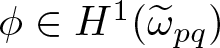 $\phi\in H^1(\widetilde {{\omega}}_{pq})$ and any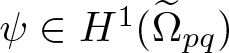 $\psi\in H^1(\widetilde {\Omega}_{pq})$, we have (see Lemma 3.3 in [Reference Chakrabortty, Griso and Orlik5])
 \begin{equation}
\begin{aligned}
&\|\phi\|_{L^2(\widetilde {{\omega}}_{pq})}\leq C\big(\|\phi\|_{L^2({\omega}^H_{pq})}+\delta\|\nabla \phi\|_{L^2(\widetilde {{\omega}}_{pq})}\big),\\
&\|\psi\|_{L^2(\widetilde {\Omega}_{pq})}\leq C\big( \|\psi\|_{L^2(\Omega^H_{pq})}+\delta\|\nabla \psi\|_{L^2(\widetilde {\Omega}_{pq})}\big).
\end{aligned}
\end{equation}
\begin{equation}
\begin{aligned}
&\|\phi\|_{L^2(\widetilde {{\omega}}_{pq})}\leq C\big(\|\phi\|_{L^2({\omega}^H_{pq})}+\delta\|\nabla \phi\|_{L^2(\widetilde {{\omega}}_{pq})}\big),\\
&\|\psi\|_{L^2(\widetilde {\Omega}_{pq})}\leq C\big( \|\psi\|_{L^2(\Omega^H_{pq})}+\delta\|\nabla \psi\|_{L^2(\widetilde {\Omega}_{pq})}\big).
\end{aligned}
\end{equation} The constant does not depend on  $\varepsilon$ and $\delta$.
Step 2. We prove (4.7).
Consider the function  ${\boldsymbol\phi}_{pq}=\mathfrak{R}-\textbf{R}_{pq}$ in $\widetilde {\omega}_{pq}$, for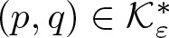 $(p,q)\in {\mathcal K}^*_\varepsilon$. First, observe that (4.6) yields ${\partial}_{\alpha}\mathfrak{V}=\textbf{R}_{pq}\textbf{e}_{\alpha}$ a.e. in ${\omega}^H_{pq}$. Therefore, this identity and (4.5) $_4$ give
 \begin{equation*}\sum_{(p,q)\in {\mathcal K}^*_\varepsilon}\big\|(\mathfrak{R}-\textbf{R}_{pq})\textbf{e}_{\alpha}\big\|^2_{L^2({\omega}^H_{pq})}\leq {C\over \delta}\textbf{D}(v)^2,\end{equation*}
which, combined with (4.9) $_1$ and using (4.5) $_3$, yields
 \begin{equation}
\sum_{(p,q)\in {\mathcal K}^*_\varepsilon}\|{\boldsymbol\phi}_{pq}\textbf{e}_{\alpha}\|^2_{L^2({\omega}^H_{pq})}=\sum_{(p,q)\in {\mathcal K}^*_\varepsilon}\|(\mathfrak{R}-\textbf{R}_{pq})\textbf{e}_{\alpha}\|^2_{L^2(\widetilde {\omega}_{pq})}\leq {C\over \delta}\textbf{D}(v)^2.
\end{equation}
\begin{equation}
\sum_{(p,q)\in {\mathcal K}^*_\varepsilon}\|{\boldsymbol\phi}_{pq}\textbf{e}_{\alpha}\|^2_{L^2({\omega}^H_{pq})}=\sum_{(p,q)\in {\mathcal K}^*_\varepsilon}\|(\mathfrak{R}-\textbf{R}_{pq})\textbf{e}_{\alpha}\|^2_{L^2(\widetilde {\omega}_{pq})}\leq {C\over \delta}\textbf{D}(v)^2.
\end{equation} Since both  $\mathfrak{R}$ and $\textbf{R}_{pq}$ belong to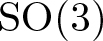 $\mathrm{SO}(3)$, we have $|\mathfrak{R}|_F=|\textbf{R}_{pq}|_F=\sqrt{3}$ and
 \begin{equation*}{\boldsymbol\phi}_{pq}\textbf{e}_3=(\mathfrak{R}-\textbf{R}_{pq})\textbf{e}_3=(\mathfrak{R}-\textbf{R}_{pq})\textbf{e}_1\land\mathfrak{R}\textbf{e}_2+\textbf{R}_{pq}\textbf{e}_1\land(\mathfrak{R}-\textbf{R}_{pq})\textbf{e}_2,\end{equation*}
which, together with (4.10), gives (4.7) $_1$. Then, as a consequence of (4.7) $_1$ and (4.5) $_5$, we obtain (4.7) $_2$.
$_2$.
Similarly, we set  $\phi_{pq}(x)=v(x)-a_{pq}-\textbf{R}_{pq}\overline{x}_{pq}$ in $\widetilde \Omega_{pq}$, for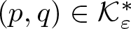 $(p,q)\in {\mathcal K}^*_\varepsilon$. Using the fact that $v(x)=\textbf{a}_{pq}+\textbf{R}_{pq}\overline{x}_{pq}$ a.e. in $\Omega^H_{pq}$, i.e.,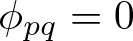 $\phi_{pq}=0$ a.e. in $\Omega^H_{pq}$, and estimate (4.7) $_2$ together with (4.9) $_2$, we obtain
 \begin{equation*}\|\phi_{pq}\|_{L^2(\widetilde \Omega_{pq})}\leq C\delta\|\nabla v-\textbf{R}_{pq}\|_{L^2(\widetilde \Omega_{pq})}.\end{equation*}
 Hence, after summation we obtain (4.7) $_3$.
$_3$.
Step 3. We prove (4.8).
Observe that, using (4.6) and (4.9) $_1$, we have
 \begin{equation*}\int_{\widetilde {{\omega}}_{pq}}\big|\mathfrak{V}-a_{pq}-\textbf{R}_{pq}\overline{x}^{'}_{pq}\big|^2dx'\leq C\delta^2\sum_{{\alpha}=1}^2\|{\partial}_{\alpha}\mathfrak{V}-\textbf{R}_{pq}\textbf{e}_{\alpha}\|^2_{L^2(\widetilde {\omega}_{pq})},\end{equation*}
which, together with (4.5) $_3$ and (4.7) $_1$, yields (4.8). This completes the proof.
As a consequence of the above lemma, we obtain the following result.
Lemma 4.4. We have
 \begin{equation}
\begin{aligned}
& \sum_{p=1}^{N_\varepsilon-1}\sum_{q=0}^{N_\varepsilon-1}|\mathbf{R}_{pq}-\mathbf{R}_{p-1q}|^2\leq {C\over \varepsilon\delta^2}\mathbf{D}(v)^2,\\
& \sum_{q=1}^{N_\varepsilon-1}\sum_{p=0}^{N_\varepsilon-1}|\mathbf{R}_{pq}-\mathbf{R}_{pq-1}|^2\leq {C\over \varepsilon\delta^2}\mathbf{D}(v)^2,\\\
&\sum_{p=1}^{N_\varepsilon-1}\sum_{q=0}^{N_\varepsilon-1}|(\mathbf{R}_{pq}-\mathbf{R}_{p-1q})\mathbf{e}_2|^2\leq {C\over \varepsilon^3}\mathbf{D}(v)^2,\\ &\sum_{q=1}^{N_\varepsilon-1}\sum_{p=0}^{N_\varepsilon-1}|(\mathbf{R}_{pq}-\mathbf{R}_{pq-1})\mathbf{e}_1|^2\leq {C\over \varepsilon^3}\mathbf{D}(v)^2,\\
& \sum_{q=0}^{N_\varepsilon-1}\sum_{p=1}^{N_\varepsilon-1}|\mathbf{a}_{pq}-\mathbf{a}_{p-1q}-\varepsilon\mathbf{R}_{p-1q}\mathbf{e}_1|^2\\
&\quad + \sum_{p=0}^{N_\varepsilon-1}\sum_{q=1}^{N_\varepsilon-1}|\mathbf{a}_{pq}-\mathbf{a}_{pq-1}-\varepsilon\mathbf{R}_{pq-1}\mathbf{e}_2|^2\leq {C\over \varepsilon}\mathbf{D}(v)^2.
\end{aligned}
\end{equation}
\begin{equation}
\begin{aligned}
& \sum_{p=1}^{N_\varepsilon-1}\sum_{q=0}^{N_\varepsilon-1}|\mathbf{R}_{pq}-\mathbf{R}_{p-1q}|^2\leq {C\over \varepsilon\delta^2}\mathbf{D}(v)^2,\\
& \sum_{q=1}^{N_\varepsilon-1}\sum_{p=0}^{N_\varepsilon-1}|\mathbf{R}_{pq}-\mathbf{R}_{pq-1}|^2\leq {C\over \varepsilon\delta^2}\mathbf{D}(v)^2,\\\
&\sum_{p=1}^{N_\varepsilon-1}\sum_{q=0}^{N_\varepsilon-1}|(\mathbf{R}_{pq}-\mathbf{R}_{p-1q})\mathbf{e}_2|^2\leq {C\over \varepsilon^3}\mathbf{D}(v)^2,\\ &\sum_{q=1}^{N_\varepsilon-1}\sum_{p=0}^{N_\varepsilon-1}|(\mathbf{R}_{pq}-\mathbf{R}_{pq-1})\mathbf{e}_1|^2\leq {C\over \varepsilon^3}\mathbf{D}(v)^2,\\
& \sum_{q=0}^{N_\varepsilon-1}\sum_{p=1}^{N_\varepsilon-1}|\mathbf{a}_{pq}-\mathbf{a}_{p-1q}-\varepsilon\mathbf{R}_{p-1q}\mathbf{e}_1|^2\\
&\quad + \sum_{p=0}^{N_\varepsilon-1}\sum_{q=1}^{N_\varepsilon-1}|\mathbf{a}_{pq}-\mathbf{a}_{pq-1}-\varepsilon\mathbf{R}_{pq-1}\mathbf{e}_2|^2\leq {C\over \varepsilon}\mathbf{D}(v)^2.
\end{aligned}
\end{equation} The constants do not depend on  $\varepsilon$, $\delta$, and $L$.
$L$.
Proof. First, we set
 \begin{equation}
\widetilde {\Omega}_{pq}\doteq \widetilde {{\omega}}_{pq} \times {\mathfrak{I}}_\delta,\quad\forall\, (p,q)\in {\mathcal K}^*_\varepsilon.
\end{equation}
\begin{equation}
\widetilde {\Omega}_{pq}\doteq \widetilde {{\omega}}_{pq} \times {\mathfrak{I}}_\delta,\quad\forall\, (p,q)\in {\mathcal K}^*_\varepsilon.
\end{equation}The proof is organized into the following steps.
Step 1. We recall the following classical result. For any 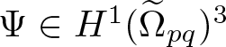 $\Psi\in H^1(\widetilde {\Omega}_{pq})^3$, we have
 \begin{equation}
\begin{aligned}
&\|\Psi\|_{L^2(\widetilde {\Omega}_{pq})}\leq C\big(\|\Psi\|_{L^2(\Omega^H_{pq})}+\delta\|\mathrm{dist}(\nabla\Psi;\mathrm{SO}(3))\|_{L^2(\widetilde {\Omega}_{pq})}\big).
\end{aligned}
\end{equation}
\begin{equation}
\begin{aligned}
&\|\Psi\|_{L^2(\widetilde {\Omega}_{pq})}\leq C\big(\|\Psi\|_{L^2(\Omega^H_{pq})}+\delta\|\mathrm{dist}(\nabla\Psi;\mathrm{SO}(3))\|_{L^2(\widetilde {\Omega}_{pq})}\big).
\end{aligned}
\end{equation} The constant does not depend on  $\varepsilon$ and $\delta$.
Below, we provide a brief proof of this inequality. Theorem II.1.1 in [Reference Blanchard and Griso1] yields a rigid deformation  $\textbf{S}_{pq}={\mathcal{G}}_{pq}+\textbf{B}_{pq}\land \overline{x}_{pq}$, $({\mathcal{G}}_{pq},\textbf{B}_{pq})\in {\mathbb{R}}^3\times \mathrm{SO}(3)$ such that
 \begin{equation*}\|\Psi-\textbf{S}_{pq}\|_{L^2(\widetilde {\Omega}_{pq})}\leq C\delta \|\mathrm{dist}(\nabla\Psi;\mathrm{SO}(3))\|_{L^2(\widetilde {\Omega}_{pq})}.\end{equation*}
Thus,
 \begin{equation*}\begin{aligned}
\|\Psi\|^2_{L^2(\widetilde {\Omega}_{pq})}\leq C\big(\|\textbf{S}_{pq}\|^2_{L^2(\widetilde {\Omega}_{pq})}+\delta^2\|\mathrm{dist}(\nabla\Psi;\mathrm{SO}(3))\|^2_{L^2(\widetilde {\Omega}_{pq})}\big)\\
\leq C\big((\varepsilon+\delta)^2|{\mathcal{G}}_{pq}|^2+(\varepsilon+\delta)^4|\textbf{B}_{pq}|^2 +\delta^2\|\mathrm{dist}(\nabla\Psi;\mathrm{SO}(3))\|^2_{L^2(\widetilde {\Omega}_{pq})}\big).
\end{aligned}
\end{equation*}
\begin{equation*}\begin{aligned}
\|\Psi\|^2_{L^2(\widetilde {\Omega}_{pq})}\leq C\big(\|\textbf{S}_{pq}\|^2_{L^2(\widetilde {\Omega}_{pq})}+\delta^2\|\mathrm{dist}(\nabla\Psi;\mathrm{SO}(3))\|^2_{L^2(\widetilde {\Omega}_{pq})}\big)\\
\leq C\big((\varepsilon+\delta)^2|{\mathcal{G}}_{pq}|^2+(\varepsilon+\delta)^4|\textbf{B}_{pq}|^2 +\delta^2\|\mathrm{dist}(\nabla\Psi;\mathrm{SO}(3))\|^2_{L^2(\widetilde {\Omega}_{pq})}\big).
\end{aligned}
\end{equation*}Besides, we have
 \begin{equation*}(\varepsilon-\delta)^2|{\mathcal{G}}_{pq}|^2+(\varepsilon-\delta)^4|\textbf{B}_{pq}|^2\leq C \|\textbf{S}_{pq}\|^2_{L^2(\Omega^H_{pq})}\leq 2\big(\|\Psi-\textbf{S}_{pq}\|^2_{L^2(\Omega^H_{pq})}+\|\Psi\|^2_{L^2(\Omega^H_{pq})}\big).\end{equation*}
This completes the proof of (4.13).
Step 2. A preliminary result.
Let  $v$ and $w$ be two rigid deformations
 \begin{equation*}
v(x)=\textbf{a}+\textbf{R} \left(\begin{matrix}
x_1\\
x_2\\
x_3
\end{matrix}\right) \text{a.e. in } \Big(-{\delta\over 2},\varepsilon\Big)\times {\mathfrak{I}}_\varepsilon\times {\mathfrak{I}}_\delta,\quad (\textbf{a},\textbf{R})\in{\mathbb{R}}^3\times \mathrm{SO}(3)
\end{equation*}
\begin{equation*}
v(x)=\textbf{a}+\textbf{R} \left(\begin{matrix}
x_1\\
x_2\\
x_3
\end{matrix}\right) \text{a.e. in } \Big(-{\delta\over 2},\varepsilon\Big)\times {\mathfrak{I}}_\varepsilon\times {\mathfrak{I}}_\delta,\quad (\textbf{a},\textbf{R})\in{\mathbb{R}}^3\times \mathrm{SO}(3)
\end{equation*}and
 \begin{equation*}
w(x)=\textbf{a}^{'}+\textbf{R}^{'}\left(\begin{matrix}
x_1+\varepsilon\\
x_2\\
x_3
\end{matrix}\right) \text{a.e. in } \Big(-\varepsilon,{\delta\over 2}\Big)\times {\mathfrak{I}}_\varepsilon\times {\mathfrak{I}}_\delta,\quad (\textbf{a}^{'},\textbf{R}^{'})\in{\mathbb{R}}^3\times \mathrm{SO}(3).
\end{equation*}
\begin{equation*}
w(x)=\textbf{a}^{'}+\textbf{R}^{'}\left(\begin{matrix}
x_1+\varepsilon\\
x_2\\
x_3
\end{matrix}\right) \text{a.e. in } \Big(-\varepsilon,{\delta\over 2}\Big)\times {\mathfrak{I}}_\varepsilon\times {\mathfrak{I}}_\delta,\quad (\textbf{a}^{'},\textbf{R}^{'})\in{\mathbb{R}}^3\times \mathrm{SO}(3).
\end{equation*} In  $\displaystyle {\mathcal{O}}_{{\varepsilon\delta}}\doteq{\mathfrak{I}}_\delta\times {\mathfrak{I}}_\varepsilon\times {\mathfrak{I}}_\delta$, we have
 \begin{equation*}
\begin{aligned}
\textbf{u}&=v-w=\textbf{a}-\textbf{a}^{'}-\varepsilon\textbf{R}^{'}\textbf{e}_1+(\textbf{R}-\textbf{R}^{'})x.
\end{aligned}
\qquad \hbox{in }\; {\mathcal{O}}_{{\varepsilon\delta}}.
\end{equation*}
\begin{equation*}
\begin{aligned}
\textbf{u}&=v-w=\textbf{a}-\textbf{a}^{'}-\varepsilon\textbf{R}^{'}\textbf{e}_1+(\textbf{R}-\textbf{R}^{'})x.
\end{aligned}
\qquad \hbox{in }\; {\mathcal{O}}_{{\varepsilon\delta}}.
\end{equation*} The  $L^2$ norm of $v-w$ in ${\mathcal{O}}_{\varepsilon\delta}$ is given by
 \begin{equation}
\begin{aligned}
{1\over \varepsilon\delta^2}\|\textbf{u}\|^2_{L^2({\mathcal{O}}_{{\varepsilon\delta}})}&=\Big|\textbf{a}-\textbf{a}^{'}-\varepsilon\textbf{R}^{'}\textbf{e}_1\Big|^2
+ {\delta^2\over 6}|(\textbf{R}-\textbf{R}^{'})\textbf{e}_1|^2\\
&\quad +{\delta^2\over 6}|(\textbf{R}-\textbf{R}^{'})\textbf{e}_3|^2+\Big({\varepsilon^2\over 12}+{\delta^2\over 12}\Big)|(\textbf{R}-\textbf{R}^{'})\textbf{e}_2|^2.
\end{aligned}
\end{equation}
\begin{equation}
\begin{aligned}
{1\over \varepsilon\delta^2}\|\textbf{u}\|^2_{L^2({\mathcal{O}}_{{\varepsilon\delta}})}&=\Big|\textbf{a}-\textbf{a}^{'}-\varepsilon\textbf{R}^{'}\textbf{e}_1\Big|^2
+ {\delta^2\over 6}|(\textbf{R}-\textbf{R}^{'})\textbf{e}_1|^2\\
&\quad +{\delta^2\over 6}|(\textbf{R}-\textbf{R}^{'})\textbf{e}_3|^2+\Big({\varepsilon^2\over 12}+{\delta^2\over 12}\Big)|(\textbf{R}-\textbf{R}^{'})\textbf{e}_2|^2.
\end{aligned}
\end{equation}Step 3. We prove (4.11).
We apply (4.13) with the deformations  $v=u$ and $w_{pq}=\textbf{a}_{pq}+\textbf{R}_{pq}\overline{x}_{pq}$ in $\widetilde {\Omega}_{pq}$. We then apply it with $v=u$ and $w_{p-1q}=\textbf{a}_{p-1q}+\textbf{R}_{p-1q} \overline{x}_{p-1q}$ in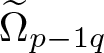 $\widetilde {\Omega}_{p-1q}$. This allows us to estimate $w_{pq}-w_{p-1q}$ in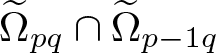 $\widetilde {\Omega}_{pq}\cap \widetilde {\Omega}_{p-1q}$ using (4.14). We obtain (4.11) $_{1,3,7}$. Similarly, proceeding as above, we estimate $w_{pq}-w_{pq-1}$ in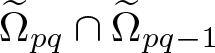 $\widetilde {\Omega}_{pq}\cap \widetilde {\Omega}_{pq-1}$, which, together with (4.14), yields (4.11) $_{2,4,8}$.
4.2. Decomposition of the deformation of thin plate reinforced with rigid inclusions
In this subsection, we construct and give estimates for the global fields in  $\Omega_{\delta}$. Before presenting the main decomposition result, we construct supporting fields $\textbf{R}^\circ$, $\textbf{R}^{\diamond}$, and ${\mathcal{V}}^{\diamond}$, which are necessary to get sharp estimates for the global fields in the main decomposition. Moreover, these supporting fields are necessary for the asymptotic analysis and to get optimal regularity for the macroscopic fields.
4.2.1. The supporting fields
$\textbf{R}^\circ$,
$\textbf{R}^{\diamond}$, and
${\mathcal{V}}^{\diamond}$


Let 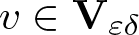 $v\in\textbf{V}_{\varepsilon\delta}$ satisfy (3.2), then from the previous subsection, we have the decomposition (4.2) for $v$ satisfying (4.3)–(4.5) and we have the estimates (4.7), (4.8), and (4.11).
First, we need to define  $\textbf{a}_{pq}$ and $\textbf{R}_{pq}$ for all $(p,q)\in \overline{{\mathcal{K}}}_\varepsilon\setminus {\mathcal{K}}^*_\varepsilon$. For that, we set (We use $ \textbf{R}_{pq} $ and $ \textbf{R}_{p,q} $ interchangeably for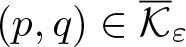 $ (p,q) \in \overline{\mathcal{K}}_\varepsilon $, as they refer to the same field. Similarly, $ \textbf{a}_{pq} $ and $ \textbf{a}_{p,q} $ are used to denote the same quantity.)
 \begin{equation*}
\begin{aligned}
&\textbf{a}_{-1,q}=\textbf{a}_{0,q},\, \textbf{R}_{-1,q}=\textbf{R}_{0,q},\, \textbf{a}_{p,q}=\textbf{a}_{N_\varepsilon-1,q},\, \textbf{R}_{p,q}=\textbf{R}_{N_\varepsilon-1,q},\\
&\quad q\in\{0,\ldots,N_\varepsilon-1\},\,p\in\{N_\varepsilon,N_\varepsilon+1\},\\
&\textbf{a}_{p,-1}=\textbf{a}_{p,0},\, \textbf{R}_{p,-1}=\textbf{R}_{p,0},\, \textbf{a}_{p,N_\varepsilon}=\textbf{a}_{p,N_\varepsilon-1},\, \textbf{R}_{p,N_\varepsilon}=\textbf{R}_{p,N_\varepsilon-1},\\
&\quad p\in\{-1,\ldots,N_\varepsilon+1\}.
\end{aligned}
\end{equation*}
\begin{equation*}
\begin{aligned}
&\textbf{a}_{-1,q}=\textbf{a}_{0,q},\, \textbf{R}_{-1,q}=\textbf{R}_{0,q},\, \textbf{a}_{p,q}=\textbf{a}_{N_\varepsilon-1,q},\, \textbf{R}_{p,q}=\textbf{R}_{N_\varepsilon-1,q},\\
&\quad q\in\{0,\ldots,N_\varepsilon-1\},\,p\in\{N_\varepsilon,N_\varepsilon+1\},\\
&\textbf{a}_{p,-1}=\textbf{a}_{p,0},\, \textbf{R}_{p,-1}=\textbf{R}_{p,0},\, \textbf{a}_{p,N_\varepsilon}=\textbf{a}_{p,N_\varepsilon-1},\, \textbf{R}_{p,N_\varepsilon}=\textbf{R}_{p,N_\varepsilon-1},\\
&\quad p\in\{-1,\ldots,N_\varepsilon+1\}.
\end{aligned}
\end{equation*} Since 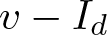 $v-I_d$ vanishes on $\Gamma_\delta$, we set
 \begin{equation*}\begin{aligned}
&\textbf{a}_{-1,q}=-\varepsilon\textbf{e}_1+q\varepsilon\textbf{e}_2,\,&&\textbf{a}_{0,q}=q\varepsilon\textbf{e}_2,\quad \textbf{R}_{-1,q}=\textbf{R}_{0,q}=\textbf{I}_3,\quad q\in\{0,\ldots,n_\varepsilon-1\},\\
&\textbf{a}_{p,-1}=p\varepsilon\textbf{e}_1-\varepsilon\textbf{e}_2,\,&&\textbf{a}_{p,0}=p\varepsilon\textbf{e}_1,\quad \textbf{R}_{p,-1}=\textbf{R}_{p,0}=\textbf{I}_3,\quad p\in\{-1,\ldots,n_\varepsilon-1\}.
\end{aligned}
\end{equation*}
\begin{equation*}\begin{aligned}
&\textbf{a}_{-1,q}=-\varepsilon\textbf{e}_1+q\varepsilon\textbf{e}_2,\,&&\textbf{a}_{0,q}=q\varepsilon\textbf{e}_2,\quad \textbf{R}_{-1,q}=\textbf{R}_{0,q}=\textbf{I}_3,\quad q\in\{0,\ldots,n_\varepsilon-1\},\\
&\textbf{a}_{p,-1}=p\varepsilon\textbf{e}_1-\varepsilon\textbf{e}_2,\,&&\textbf{a}_{p,0}=p\varepsilon\textbf{e}_1,\quad \textbf{R}_{p,-1}=\textbf{R}_{p,0}=\textbf{I}_3,\quad p\in\{-1,\ldots,n_\varepsilon-1\}.
\end{aligned}
\end{equation*} Now, we define the fields  $\textbf{R}^{\circ}$, $\textbf{R}^\diamond$, and ${\mathcal{V}}^{\diamond}$ by
 \begin{equation*}
\begin{aligned}
&\textbf{R}^\circ=\textbf{R}_{pq}\quad \hbox{a.e. in }\; {\omega}_{pq},\quad (p,q)\in \overline{{\mathcal{K}}}_\varepsilon,\\
&\textbf{R}^\diamond(p\varepsilon,q\varepsilon)=\textbf{R}_{pq},\quad {\mathcal{V}}^{\diamond}(p\varepsilon,q\varepsilon)=\textbf{a}_{pq},\quad (p,q)\in\overline{{\mathcal K}}_\varepsilon,
\end{aligned}
\end{equation*}
\begin{equation*}
\begin{aligned}
&\textbf{R}^\circ=\textbf{R}_{pq}\quad \hbox{a.e. in }\; {\omega}_{pq},\quad (p,q)\in \overline{{\mathcal{K}}}_\varepsilon,\\
&\textbf{R}^\diamond(p\varepsilon,q\varepsilon)=\textbf{R}_{pq},\quad {\mathcal{V}}^{\diamond}(p\varepsilon,q\varepsilon)=\textbf{a}_{pq},\quad (p,q)\in\overline{{\mathcal K}}_\varepsilon,
\end{aligned}
\end{equation*}and in  $\overline{{\omega}}_{pq}$,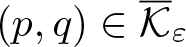 $(p,q)\in \overline{{\mathcal{K}}}_\varepsilon$, the fields $\textbf{R}^\diamond$, ${\mathcal{V}}^{\diamond}$ are the ${\mathcal{Q}}_1$ interpolation of their values at the vertices of this square. For a detailed description of ${\cal Q}_1$-interpolation, see [Reference Cioranescu, Damlamian and Griso14, Chapter 1]. By construction, we have $\textbf{R}^\circ\in L^2((-\varepsilon,L+\varepsilon))^{3\times 3}$, $\textbf{R}^\diamond\in H^1((-\varepsilon,L+\varepsilon))^{3\times 3}$, ${\mathcal{V}}^{\diamond}\in H^1((-\varepsilon,L+\varepsilon))^3$ and satisfy the following boundary conditions:
 \begin{equation*}\textbf{R}^\diamond=\textbf{I}_3,\quad {\mathcal{V}}^{\diamond}=I_d,\quad \text{in}\ (-\varepsilon,0)\times (-\varepsilon,l)\cup (-\varepsilon,l)\times (-\varepsilon,0).\end{equation*}
 Before we give the estimates for the above defined fields, we give some preliminary results for  $\textbf{R}^\circ$ and $\textbf{R}^{\diamond}$ restricted in ${\omega}_\delta$.
Lemma 4.5. There exist constants independent of  $\varepsilon$ and $\delta$ such that
 \begin{equation}
\begin{aligned}
\|\mathbf{R}^\circ-\mathbf{I}_3\|_{L^4({\omega}_\delta)}\leq C\|\mathbf{R}^\diamond-\mathbf{I}_3\|_{L^4({\omega}_\delta)} \leq C\|\mathbf{R}^\diamond-\mathbf{I}_3\|_{H^1({\omega}_\delta)}.
\end{aligned}
\end{equation}
\begin{equation}
\begin{aligned}
\|\mathbf{R}^\circ-\mathbf{I}_3\|_{L^4({\omega}_\delta)}\leq C\|\mathbf{R}^\diamond-\mathbf{I}_3\|_{L^4({\omega}_\delta)} \leq C\|\mathbf{R}^\diamond-\mathbf{I}_3\|_{H^1({\omega}_\delta)}.
\end{aligned}
\end{equation}Proof. Step 1: We prove (4.15) $_1$.
$_1$.
Set 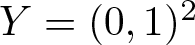 $Y=(0,1)^2$. Since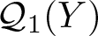 ${\mathcal{Q}}_1(Y)$, the space of ${\mathcal{Q}}_1$ interpolate functions, is finite-dimensional, there exists a strictly positive constant $M$ such that
 \begin{equation*}
|F(0,0)| \le M\,\|F\|_{L^4(Y)},\qquad \forall F\in {\mathcal{Q}}_1(Y).
\end{equation*}
\begin{equation*}
|F(0,0)| \le M\,\|F\|_{L^4(Y)},\qquad \forall F\in {\mathcal{Q}}_1(Y).
\end{equation*}By change of variables, we get
 \begin{equation*}
|F(p\varepsilon,q\varepsilon)| \le {M\over \varepsilon^{1/2}}\|F\|_{L^4({\omega}_{pq})},\quad \forall\,F\in{\mathcal{Q}}_1({\omega}_{pq}),\quad (p,q)\in\overline{{\mathcal K}}_\varepsilon.
\end{equation*}
\begin{equation*}
|F(p\varepsilon,q\varepsilon)| \le {M\over \varepsilon^{1/2}}\|F\|_{L^4({\omega}_{pq})},\quad \forall\,F\in{\mathcal{Q}}_1({\omega}_{pq}),\quad (p,q)\in\overline{{\mathcal K}}_\varepsilon.
\end{equation*} Then, the above inequality, combined with the definition of  $\textbf{R}^\circ$ and $\textbf{R}^{\diamond}$, gives
 \begin{equation*}\|\textbf{R}^\circ-\textbf{I}_3\|^4_{L^4({\omega}_{pq})}=\varepsilon^2|\textbf{R}_{pq}-\textbf{I}_3|^4\leq \varepsilon^2\left({M\over \varepsilon^{1/2}}\right)^4\|\textbf{R}^{\diamond}-\textbf{I}_3\|^4_{L^4({\omega}_{pq})}.\end{equation*}
 So, summing over all 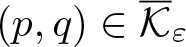 $(p,q)\in\overline{{\mathcal K}}_\varepsilon$ gives (4.15) $_1$.
$_1$.
Step 2: We prove (4.15) $_2$.
$_2$.
Since 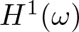 $H^1({\omega})$ is continuously embedded in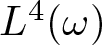 $L^4({\omega})$, there exists a strictly positive constant $C$ such that
 \begin{equation*}\|\phi\|_{L^4({\omega})}\leq C\|\phi\|_{H^1({\omega})},\qquad \forall \phi\in H^1({\omega}).\end{equation*}
 Now, let  $\psi$ be in $H^1\big((-\varepsilon,L+\varepsilon)^2\big)$. By a dilation with centre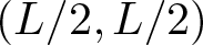 $(L/2,L/2)$ and ratio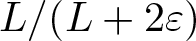 $L/(L+2\varepsilon)$, we transform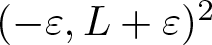 $(-\varepsilon,L+\varepsilon)^2$ into ${\omega}$. Then, after an obvious change of variables, we apply the above inequality, and again by a simple change of variables, we return to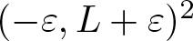 $(-\varepsilon, L+\varepsilon)^2$. This gives
 \begin{equation*}
\|\psi\|_{L^4((-\varepsilon,L+\varepsilon)^2)}\leq C\|\psi\|_{H^1((-\varepsilon,L+\varepsilon)^2)},\qquad \forall \psi\in H^1((-\varepsilon,L+\varepsilon)^2).
\end{equation*}
\begin{equation*}
\|\psi\|_{L^4((-\varepsilon,L+\varepsilon)^2)}\leq C\|\psi\|_{H^1((-\varepsilon,L+\varepsilon)^2)},\qquad \forall \psi\in H^1((-\varepsilon,L+\varepsilon)^2).
\end{equation*} The constant is independent of  $\varepsilon$. Applying this result leads to (4.15) $_2$. This completes the proof.
In the lemma below, we give estimates of the restrictions of these fields to  ${\omega}_\delta$.
Lemma 4.6. We have
 \begin{equation}
\|\nabla \mathbf{R}^\diamond\|_{L^2({\omega}_\delta)}+ \|\mathbf{R}^\diamond-\mathbf{I}_3\|_{L^2({\omega}_\delta)}\leq {C\over \varepsilon^{1/2}\delta}\mathbf{D}(v),\quad \|\partial_\alpha\mathbf{R}^\diamond\mathbf{e}_{3-\alpha}\|_{L^2({\omega}_\delta)}\leq {C\over \varepsilon^{3/2}}\mathbf{D}(v),
\end{equation}
\begin{equation}
\|\nabla \mathbf{R}^\diamond\|_{L^2({\omega}_\delta)}+ \|\mathbf{R}^\diamond-\mathbf{I}_3\|_{L^2({\omega}_\delta)}\leq {C\over \varepsilon^{1/2}\delta}\mathbf{D}(v),\quad \|\partial_\alpha\mathbf{R}^\diamond\mathbf{e}_{3-\alpha}\|_{L^2({\omega}_\delta)}\leq {C\over \varepsilon^{3/2}}\mathbf{D}(v),
\end{equation}and
 \begin{equation}
\|{\partial}_{\alpha}{\mathcal{V}}^{\diamond}-\mathbf{R}^\circ\mathbf{e}_{\alpha}\|_{L^2({\omega}_\delta)}\leq {C\over \varepsilon^{1/2}}\mathbf{D}(v),\quad \|{\mathcal{V}}^{\diamond}-I_d\|_{H^1({\omega}_\delta)}\leq {C\over \varepsilon^{1/2}\delta}\mathbf{D}(v).
\end{equation}
\begin{equation}
\|{\partial}_{\alpha}{\mathcal{V}}^{\diamond}-\mathbf{R}^\circ\mathbf{e}_{\alpha}\|_{L^2({\omega}_\delta)}\leq {C\over \varepsilon^{1/2}}\mathbf{D}(v),\quad \|{\mathcal{V}}^{\diamond}-I_d\|_{H^1({\omega}_\delta)}\leq {C\over \varepsilon^{1/2}\delta}\mathbf{D}(v).
\end{equation}Moreover, we have
 \begin{equation}
\begin{aligned}
\|\mathbf{R}^{\diamond}(\mathbf{R}^{\diamond})^T-\mathbf{I}_3\|_{L^2({\omega}_\delta)} \leq {C\varepsilon^{1/2}\over \delta}\mathbf{D}(v),\qquad \|(\mathbf{R}^\circ)^T+\mathbf{R}^\circ-2\mathbf{I}_3\|_{L^2({\omega}_\delta)} \leq {C\over \varepsilon\delta^2}\mathbf{D}(v)^2.
\end{aligned}
\end{equation}
\begin{equation}
\begin{aligned}
\|\mathbf{R}^{\diamond}(\mathbf{R}^{\diamond})^T-\mathbf{I}_3\|_{L^2({\omega}_\delta)} \leq {C\varepsilon^{1/2}\over \delta}\mathbf{D}(v),\qquad \|(\mathbf{R}^\circ)^T+\mathbf{R}^\circ-2\mathbf{I}_3\|_{L^2({\omega}_\delta)} \leq {C\over \varepsilon\delta^2}\mathbf{D}(v)^2.
\end{aligned}
\end{equation} Furthermore, for the corresponding displacement  ${\mathcal{U}}^{\diamond}={\mathcal{V}}^{\diamond}-I_d$, we have
 \begin{equation}
\|{\mathcal{U}}^{\diamond}_3\|_{H^1({\omega}_\delta)}\leq {C\over \varepsilon^{1/2}\delta}\mathbf{D}(v),\qquad \|{\mathcal{U}}^{\diamond}_{\alpha}\|_{H^1({\omega}_\delta)}\leq {C\over \varepsilon^{1/2}}\mathbf{D}(v)\left(1+{\mathbf{D}(v)\over \varepsilon^{1/2}\delta^2}\right).
\end{equation}
\begin{equation}
\|{\mathcal{U}}^{\diamond}_3\|_{H^1({\omega}_\delta)}\leq {C\over \varepsilon^{1/2}\delta}\mathbf{D}(v),\qquad \|{\mathcal{U}}^{\diamond}_{\alpha}\|_{H^1({\omega}_\delta)}\leq {C\over \varepsilon^{1/2}}\mathbf{D}(v)\left(1+{\mathbf{D}(v)\over \varepsilon^{1/2}\delta^2}\right).
\end{equation} The constants are independent of  $\varepsilon$ and $\delta$.
Proof. Step 1: We prove (4.16)–(4.17).
Using the definition of  $\textbf{R}^\diamond$, for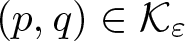 $(p,q)\in{\mathcal{K}}_\varepsilon$, we have ${\omega}_{pq}$
 \begin{equation}
\begin{aligned}
\textbf{R}^\diamond(p\varepsilon+z_1,q\varepsilon+z_2)&=\textbf{R}_{pq}{\varepsilon-z_1\over \varepsilon}{\varepsilon-z_2\over \varepsilon}+\textbf{R}_{pq+1}{(\varepsilon-z_1)z_2\over \varepsilon^2}\\
& +\textbf{R}_{p+1q}{z_1(\varepsilon-z_2)\over \varepsilon^2}+\textbf{R}_{p+1q+1}{z_1z_2\over \varepsilon^2},
\end{aligned}
\,\quad \forall\,(z_1,z_2)\in(0,\varepsilon)^2.
\end{equation}
\begin{equation}
\begin{aligned}
\textbf{R}^\diamond(p\varepsilon+z_1,q\varepsilon+z_2)&=\textbf{R}_{pq}{\varepsilon-z_1\over \varepsilon}{\varepsilon-z_2\over \varepsilon}+\textbf{R}_{pq+1}{(\varepsilon-z_1)z_2\over \varepsilon^2}\\
& +\textbf{R}_{p+1q}{z_1(\varepsilon-z_2)\over \varepsilon^2}+\textbf{R}_{p+1q+1}{z_1z_2\over \varepsilon^2},
\end{aligned}
\,\quad \forall\,(z_1,z_2)\in(0,\varepsilon)^2.
\end{equation} The estimates (4.16) $_{1,3}$ are the immediate consequences of (4.11) $_{1,2,3,4}$ and the ${\mathcal{Q}}_1$-character of $\textbf{R}^\diamond$. Then, the boundary condition satisfied by $\textbf{R}^\diamond$ leads to (4.16) $_{2}$.
Besides, we also have in  ${\omega}_{pq}$, $(z_1,z_2)\in(0,\varepsilon)^2$
 \begin{align}
{\mathcal{V}}^\diamond(p\varepsilon+z_1,q\varepsilon+z_2)&=\textbf{a}_{pq}{\varepsilon-z_1\over \varepsilon}{\varepsilon-z_2\over \varepsilon} \nonumber\\
&\quad +\textbf{a}_{pq+1}{(\varepsilon-z_1)z_2\over \varepsilon^2} +\textbf{a}_{p+1q}{z_1(\varepsilon-z_2)\over \varepsilon^2}+\textbf{a}_{p+1q+1}{z_1z_2\over \varepsilon^2}.
\end{align}
\begin{align}
{\mathcal{V}}^\diamond(p\varepsilon+z_1,q\varepsilon+z_2)&=\textbf{a}_{pq}{\varepsilon-z_1\over \varepsilon}{\varepsilon-z_2\over \varepsilon} \nonumber\\
&\quad +\textbf{a}_{pq+1}{(\varepsilon-z_1)z_2\over \varepsilon^2} +\textbf{a}_{p+1q}{z_1(\varepsilon-z_2)\over \varepsilon^2}+\textbf{a}_{p+1q+1}{z_1z_2\over \varepsilon^2}.
\end{align}Then, we obtain
 \begin{align*}
\big({\partial}_1{\mathcal{V}}^{\diamond}-\textbf{R}^\circ\textbf{e}_1\big)(p\varepsilon+z_1,q\varepsilon+z_2)&={\textbf{a}_{p+1q}-\textbf{a}_{pq}-\varepsilon\textbf{R}_{pq}\textbf{e}_1\over \varepsilon}{\varepsilon-z_2\over \varepsilon}\\
&\quad +{\textbf{a}_{p+1q+1}-\textbf{a}_{pq+1}-\varepsilon\textbf{R}_{pq+1}\textbf{e}_1\over \varepsilon}{z_2\over \varepsilon}\\
& \quad +{z_2\over \varepsilon}(\textbf{R}_{pq+1}-\textbf{R}_{pq})\textbf{e}_1,
\end{align*}
\begin{align*}
\big({\partial}_1{\mathcal{V}}^{\diamond}-\textbf{R}^\circ\textbf{e}_1\big)(p\varepsilon+z_1,q\varepsilon+z_2)&={\textbf{a}_{p+1q}-\textbf{a}_{pq}-\varepsilon\textbf{R}_{pq}\textbf{e}_1\over \varepsilon}{\varepsilon-z_2\over \varepsilon}\\
&\quad +{\textbf{a}_{p+1q+1}-\textbf{a}_{pq+1}-\varepsilon\textbf{R}_{pq+1}\textbf{e}_1\over \varepsilon}{z_2\over \varepsilon}\\
& \quad +{z_2\over \varepsilon}(\textbf{R}_{pq+1}-\textbf{R}_{pq})\textbf{e}_1,
\end{align*}which along with the inequalities (4.11) $_{3,4,5}$ give (4.17) $_1$. Similarly, we get (4.17) $_1$ for ${\alpha}=2$.
The estimate (4.17) $_2$ is a direct consequence of (4.16) $_2$, (4.17) $_1$, and Poincaré-inequality.
Step 2: We prove (4.18) $_{1}$.
Observe that
 \begin{align}
(\textbf{R}^{\diamond})^T\textbf{R}^{\diamond}-\textbf{I}_3&=(\textbf{R}^{\diamond})^T\textbf{R}^{\diamond}-(\textbf{R}_{pq})^T\textbf{R}_{pq}\nonumber\\
& \quad=(\textbf{R}^{\diamond})^T(\textbf{R}^{\diamond}-\textbf{R}_{pq})+(\textbf{R}^{\diamond}-\textbf{R}_{pq})^T\textbf{R}_{pq}.
\end{align}
\begin{align}
(\textbf{R}^{\diamond})^T\textbf{R}^{\diamond}-\textbf{I}_3&=(\textbf{R}^{\diamond})^T\textbf{R}^{\diamond}-(\textbf{R}_{pq})^T\textbf{R}_{pq}\nonumber\\
& \quad=(\textbf{R}^{\diamond})^T(\textbf{R}^{\diamond}-\textbf{R}_{pq})+(\textbf{R}^{\diamond}-\textbf{R}_{pq})^T\textbf{R}_{pq}.
\end{align} As the matrices  $\textbf{R}_{pq}$ belongs to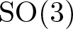 $\mathrm{SO}(3)$, the function $\textbf{R}^{\diamond}$ is uniformly bounded and satisfies
 \begin{equation*}\|\textbf{R}^{\diamond}\|_{L^\infty({\omega}_\delta)}\leq \sqrt{3}.\end{equation*}
 Again the  ${\mathcal{Q}}_1$-character of $\textbf{R}^\diamond$ together with estimate (4.16) $_{1}$ give
 \begin{equation}
\sum_{(p,q)\in {\mathcal{K}}^*_\varepsilon}\big\|\textbf{R}^\diamond -\textbf{R}_{pq}\big\|^2_{L^2({\omega}_{pq})} \leq C\varepsilon^2\|\nabla \textbf{R}^\diamond\|^2_{L^2({\omega}_\delta)}\leq C{\varepsilon\over \delta^2}\textbf{D}(v)^2.
\end{equation}
\begin{equation}
\sum_{(p,q)\in {\mathcal{K}}^*_\varepsilon}\big\|\textbf{R}^\diamond -\textbf{R}_{pq}\big\|^2_{L^2({\omega}_{pq})} \leq C\varepsilon^2\|\nabla \textbf{R}^\diamond\|^2_{L^2({\omega}_\delta)}\leq C{\varepsilon\over \delta^2}\textbf{D}(v)^2.
\end{equation} The above two inequalities along with the expression (4.22) and (4.16) $_2$ give (4.18) $_1$. Estimate (4.23) and the definition of $\textbf{R}^\circ$ also lead to
 \begin{equation}
\|\textbf{R}^{\diamond}-\textbf{R}^\circ\|_{L^2({\omega}_\delta)}\leq C{\varepsilon^{1/2}\over \delta}\textbf{D}(v),\quad \|\textbf{R}^\circ-\textbf{I}_3\|_{L^2({\omega}_\delta)}\leq {C\over \varepsilon^{1/2}\delta}\textbf{D}(v).
\end{equation}
\begin{equation}
\|\textbf{R}^{\diamond}-\textbf{R}^\circ\|_{L^2({\omega}_\delta)}\leq C{\varepsilon^{1/2}\over \delta}\textbf{D}(v),\quad \|\textbf{R}^\circ-\textbf{I}_3\|_{L^2({\omega}_\delta)}\leq {C\over \varepsilon^{1/2}\delta}\textbf{D}(v).
\end{equation} Step 3: We prove (4.18) $_2$.
$_2$.
We also have the identities
 \begin{equation}
\begin{aligned}
(\textbf{R}^\circ)^T+\textbf{R}^\circ-2\textbf{I}_3=(\textbf{R}^\circ)^T(\textbf{R}^\circ-\textbf{I}_3)^2.
\end{aligned}
\end{equation}
\begin{equation}
\begin{aligned}
(\textbf{R}^\circ)^T+\textbf{R}^\circ-2\textbf{I}_3=(\textbf{R}^\circ)^T(\textbf{R}^\circ-\textbf{I}_3)^2.
\end{aligned}
\end{equation} Then, we have (using (4.15) $_1$)
$_1$)
 \begin{equation*}\|(\textbf{R}^\circ)^T+\textbf{R}^\circ-2\textbf{I}_3\|_{L^2({\omega}_\delta)}\leq C\|\textbf{R}^\circ-\textbf{I}_3\|^2_{L^4({\omega}_\delta)}\leq C\|\textbf{R}^{\diamond}-\textbf{I}_3\|^2_{L^4({\omega}_\delta)},\end{equation*}
which combined with the continuous embedding of 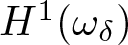 $H^1({\omega}_\delta)$ in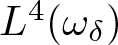 $L^4({\omega}_\delta)$ with embedding constant independent of $\varepsilon$ and $\delta$ (see (4.15)), we obtain
 \begin{equation*}
\|(\textbf{R}^\circ)^T+\textbf{R}^\circ-2\textbf{I}_3\|_{L^2({\omega}_\delta)}\leq C\|\textbf{R}^{\diamond}-\textbf{I}_3\|^2_{H^1({\omega}_\delta)}.
\end{equation*}
\begin{equation*}
\|(\textbf{R}^\circ)^T+\textbf{R}^\circ-2\textbf{I}_3\|_{L^2({\omega}_\delta)}\leq C\|\textbf{R}^{\diamond}-\textbf{I}_3\|^2_{H^1({\omega}_\delta)}.
\end{equation*} The above inequality with the estimates (4.16) $_{1,2}$ gives (4.18) $_3$.
$_3$.
Step 4: We prove (4.19).
The estimate (4.19) $_1$ is a direct consequence of (4.17) $_2$. Now, we have
 \begin{align*}
&\big(\partial_\alpha{\mathcal{V}}^{\diamond}-\textbf{R}^\circ\textbf{e}_\alpha\big)\cdot\textbf{e}_\beta+\big(\partial_\beta{\mathcal{V}}^{\diamond}-\textbf{R}^\circ\textbf{e}_\beta\big)\cdot\textbf{e}_\alpha\\
&\quad =2e_{\alpha\beta}({\mathcal{U}}^{\diamond})-\big((\textbf{R}^\circ)^T+\textbf{R}^\circ-2\textbf{I}_3\big)\textbf{e}_\beta\cdot\textbf{e}_\alpha.
\end{align*}
\begin{align*}
&\big(\partial_\alpha{\mathcal{V}}^{\diamond}-\textbf{R}^\circ\textbf{e}_\alpha\big)\cdot\textbf{e}_\beta+\big(\partial_\beta{\mathcal{V}}^{\diamond}-\textbf{R}^\circ\textbf{e}_\beta\big)\cdot\textbf{e}_\alpha\\
&\quad =2e_{\alpha\beta}({\mathcal{U}}^{\diamond})-\big((\textbf{R}^\circ)^T+\textbf{R}^\circ-2\textbf{I}_3\big)\textbf{e}_\beta\cdot\textbf{e}_\alpha.
\end{align*} Then, the above equality and (4.17) $_1$, (4.18) $_3$ imply
 \begin{equation*}\|e_{\alpha\beta}({\mathcal{U}}^{\diamond})\|_{L^2({\omega}_\delta)}\leq {C\over \varepsilon^{1/2}}\textbf{D}(v)+{C\over \varepsilon\delta^2}\textbf{D}(v)^2.\end{equation*}
 Since the  ${\mathcal{U}}^{\diamond}_\beta$’s vanish on $\gamma$, the $2D$ Korn’s inequality gives (4.56) $_2$. This completes the proof.
As a consequence,
Corollary 4.7. We have
 \begin{equation}
\|(\mathbf{R}^\circ-\mathbf{I}_3)\mathbf{e}_{\alpha}\cdot\mathbf{e}_{\beta}\|_{L^2({\omega}_\delta)}\leq {C\over \varepsilon^{1/2}}\mathbf{D}(v)\Big(1+ {\mathbf{D}(v)\over \varepsilon^{1/2}\delta^2}\Big).
\end{equation}
\begin{equation}
\|(\mathbf{R}^\circ-\mathbf{I}_3)\mathbf{e}_{\alpha}\cdot\mathbf{e}_{\beta}\|_{L^2({\omega}_\delta)}\leq {C\over \varepsilon^{1/2}}\mathbf{D}(v)\Big(1+ {\mathbf{D}(v)\over \varepsilon^{1/2}\delta^2}\Big).
\end{equation} The constant does not depend on  $\varepsilon$ and $\delta$.
Proof. From (4.17) $_1$, we have
 \begin{equation*}\|{\partial}_{\alpha}{\mathcal{U}}^{\diamond}-(\textbf{R}^\circ-\textbf{I}_3)\textbf{e}_{\alpha}\|_{L^2({\omega}_\delta)}\leq {C\over \varepsilon^{1/2}}\textbf{D}(v).\end{equation*}
Then
 \begin{equation*}(\textbf{R}^\circ-\textbf{I}_3)\textbf{e}_{\alpha}\cdot\textbf{e}_{\beta}=-\big({\partial}_{\alpha}{\mathcal{U}}^{\diamond}-(\textbf{R}^\circ-\textbf{I}_3)\textbf{e}_{\alpha}\big)\cdot\textbf{e}_{\beta}+{\partial}_{\alpha}{\mathcal{U}}^{\diamond}\cdot\textbf{e}_{\beta}\end{equation*}
Finally, we end this subsection with the following Lemma, which is a consequence of the estimates of Lemma 4.6.
Lemma 4.8. There exist  $F^{\diamond}$ and $G^{\diamond}$ in $H^1((-\varepsilon,L+\varepsilon);{\mathbb{R}}^3)$ such that
 \begin{equation}
F^{\diamond}=0,\quad G^{\diamond}=0\quad \hbox{a.e. in } (-\varepsilon,l)\quad \hbox{and}\quad \|{\mathcal{U}}^{\diamond}-F^{\diamond}-G^{\diamond}\|_{H^1({\omega}_\delta)}\leq {C\over \varepsilon^{3/2}}\mathbf{D}(v).
\end{equation}
\begin{equation}
F^{\diamond}=0,\quad G^{\diamond}=0\quad \hbox{a.e. in } (-\varepsilon,l)\quad \hbox{and}\quad \|{\mathcal{U}}^{\diamond}-F^{\diamond}-G^{\diamond}\|_{H^1({\omega}_\delta)}\leq {C\over \varepsilon^{3/2}}\mathbf{D}(v).
\end{equation}Moreover, we have
 \begin{equation}
\|(\mathbf{R}^{\diamond}-\mathbf{I}_3)\mathbf{e}_1-d_1F^{\diamond}\|_{L^2({\omega}_\delta)}+\|(\mathbf{R}^{\diamond}-\mathbf{I}_3)\mathbf{e}_2-d_2G^{\diamond}\|_{L^2({\omega}_\delta)}\leq {C\over \varepsilon^{3/2}}\mathbf{D}(v).
\end{equation}
\begin{equation}
\|(\mathbf{R}^{\diamond}-\mathbf{I}_3)\mathbf{e}_1-d_1F^{\diamond}\|_{L^2({\omega}_\delta)}+\|(\mathbf{R}^{\diamond}-\mathbf{I}_3)\mathbf{e}_2-d_2G^{\diamond}\|_{L^2({\omega}_\delta)}\leq {C\over \varepsilon^{3/2}}\mathbf{D}(v).
\end{equation} The constants do not depend on  $\varepsilon$ and $\delta$.
Proof. Using the estimates (4.16) $_3$, the directional Poincaré inequality, and the boundary conditions, we obtain
 \begin{equation}
\begin{aligned}
\|(\textbf{R}^\diamond-\textbf{I}_3)\textbf{e}_2-(\textbf{R}^\diamond-\textbf{I}_3)(-{\delta\over 2},\cdot)\textbf{e}_2\|_{L^2({\omega}_\delta)}&\leq {C\over \varepsilon^{3/2}}\textbf{D}(v) \\
\|(\textbf{R}^\diamond-\textbf{I}_3)\textbf{e}_1-(\textbf{R}^\diamond-\textbf{I}_3)(\cdot,-{\delta\over 2})\textbf{e}_1\|_{L^2({\omega}_\delta)} &\leq {C\over \varepsilon^{3/2}}\textbf{D}(v),
\end{aligned}
\end{equation}
\begin{equation}
\begin{aligned}
\|(\textbf{R}^\diamond-\textbf{I}_3)\textbf{e}_2-(\textbf{R}^\diamond-\textbf{I}_3)(-{\delta\over 2},\cdot)\textbf{e}_2\|_{L^2({\omega}_\delta)}&\leq {C\over \varepsilon^{3/2}}\textbf{D}(v) \\
\|(\textbf{R}^\diamond-\textbf{I}_3)\textbf{e}_1-(\textbf{R}^\diamond-\textbf{I}_3)(\cdot,-{\delta\over 2})\textbf{e}_1\|_{L^2({\omega}_\delta)} &\leq {C\over \varepsilon^{3/2}}\textbf{D}(v),
\end{aligned}
\end{equation}which, along with the definition of  $\textbf{R}^\diamond$, give
 \begin{equation*}\begin{aligned}
\|\textbf{R}^\diamond\textbf{e}_2-\textbf{R}^\diamond(0,\cdot)\textbf{e}_2\|_{L^2({\omega}_\delta)}&\leq {C\over \varepsilon^{3/2}}\textbf{D}(v),\\ \|\textbf{R}^\diamond\textbf{e}_1-\textbf{R}^\diamond(\cdot,0)\textbf{e}_1\|_{L^2({\omega}_\delta)}& \leq {C\over \varepsilon^{3/2}}\textbf{D}(v).
\end{aligned}
\end{equation*}
\begin{equation*}\begin{aligned}
\|\textbf{R}^\diamond\textbf{e}_2-\textbf{R}^\diamond(0,\cdot)\textbf{e}_2\|_{L^2({\omega}_\delta)}&\leq {C\over \varepsilon^{3/2}}\textbf{D}(v),\\ \|\textbf{R}^\diamond\textbf{e}_1-\textbf{R}^\diamond(\cdot,0)\textbf{e}_1\|_{L^2({\omega}_\delta)}& \leq {C\over \varepsilon^{3/2}}\textbf{D}(v).
\end{aligned}
\end{equation*} Using the definition (4.20), we have in  ${\omega}_{pq}$ for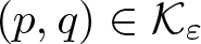 $(p,q)\in{\mathcal{K}}_\varepsilon$
 \begin{align*}
\textbf{R}^\diamond\textbf{e}_2-\textbf{R}^\diamond(0,\cdot)\textbf{e}_2 & ={\varepsilon-x_2\over \varepsilon}\left[(\textbf{R}_{p-1q-1}-\textbf{R}_{0q-1})+(\textbf{R}_{p-1q}-\textbf{R}_{0q})\right]\textbf{e}_2\\
& \quad+{\varepsilon+x_2\over \varepsilon}\left[(\textbf{R}_{pq-1}-\textbf{R}_{0q-1})
+(\textbf{R}_{pq}-\textbf{R}_{0q})\right]\textbf{e}_2\\
& \quad +{\varepsilon-x_2\over \varepsilon}{x_1\over \varepsilon}(\textbf{R}_{pq-1}-\textbf{R}_{p-1q-1})\textbf{e}_2\\
& \quad +{\varepsilon+x_2\over \varepsilon}{x_1\over \varepsilon}(\textbf{R}_{pq}-\textbf{R}_{p-1q})\textbf{e}_2
\end{align*}
\begin{align*}
\textbf{R}^\diamond\textbf{e}_2-\textbf{R}^\diamond(0,\cdot)\textbf{e}_2 & ={\varepsilon-x_2\over \varepsilon}\left[(\textbf{R}_{p-1q-1}-\textbf{R}_{0q-1})+(\textbf{R}_{p-1q}-\textbf{R}_{0q})\right]\textbf{e}_2\\
& \quad+{\varepsilon+x_2\over \varepsilon}\left[(\textbf{R}_{pq-1}-\textbf{R}_{0q-1})
+(\textbf{R}_{pq}-\textbf{R}_{0q})\right]\textbf{e}_2\\
& \quad +{\varepsilon-x_2\over \varepsilon}{x_1\over \varepsilon}(\textbf{R}_{pq-1}-\textbf{R}_{p-1q-1})\textbf{e}_2\\
& \quad +{\varepsilon+x_2\over \varepsilon}{x_1\over \varepsilon}(\textbf{R}_{pq}-\textbf{R}_{p-1q})\textbf{e}_2
\end{align*}the above equality with the estimates (4.11) $_3$ and (4.29) give
 \begin{equation*}\sum_{p=0}^{N_\varepsilon}\sum_{q=0}^{N_\varepsilon-1}\left|(\textbf{R}_{pq-1}-\textbf{R}_{0q-1})\textbf{e}_2+(\textbf{R}_{pq+1}-\textbf{R}_{0q})\textbf{e}_2\right|^2\varepsilon^2\leq {C\over \varepsilon^3}\textbf{D}(v)^2.\end{equation*}
 Similarly, proceeding for the other direction with the estimate (4.11) $_4$, we obtain
 \begin{equation*}
\sum_{(p,q)\in{\mathcal{K}}_\varepsilon^{(2)}}|(\textbf{R}_{pq}-\textbf{R}_{0q})\textbf{e}_2|^2\varepsilon^2+\sum_{(p,q)\in{\mathcal{K}}_\varepsilon^{(1)}}|(\textbf{R}_{pq}-\textbf{R}_{p0})\textbf{e}_1|^2\varepsilon^2\leq {C\over \varepsilon^3}\textbf{D}(v)^2.
\end{equation*}
\begin{equation*}
\sum_{(p,q)\in{\mathcal{K}}_\varepsilon^{(2)}}|(\textbf{R}_{pq}-\textbf{R}_{0q})\textbf{e}_2|^2\varepsilon^2+\sum_{(p,q)\in{\mathcal{K}}_\varepsilon^{(1)}}|(\textbf{R}_{pq}-\textbf{R}_{p0})\textbf{e}_1|^2\varepsilon^2\leq {C\over \varepsilon^3}\textbf{D}(v)^2.
\end{equation*}The above inequality implies
 \begin{equation}
\|\textbf{R}^\circ\textbf{e}_2-\textbf{R}^\diamond(0,\cdot)\textbf{e}_2\|_{L^2({\omega}_\delta)}\leq {C\over \varepsilon^{3/2}}\textbf{D}(v),\quad \|\textbf{R}^\circ\textbf{e}_1-\textbf{R}^\diamond(\cdot,0)\textbf{e}_1\|_{L^2({\omega}_\delta)} \leq {C\over \varepsilon^{3/2}}\textbf{D}(v).
\end{equation}
\begin{equation}
\|\textbf{R}^\circ\textbf{e}_2-\textbf{R}^\diamond(0,\cdot)\textbf{e}_2\|_{L^2({\omega}_\delta)}\leq {C\over \varepsilon^{3/2}}\textbf{D}(v),\quad \|\textbf{R}^\circ\textbf{e}_1-\textbf{R}^\diamond(\cdot,0)\textbf{e}_1\|_{L^2({\omega}_\delta)} \leq {C\over \varepsilon^{3/2}}\textbf{D}(v).
\end{equation}Now, we set
 \begin{equation*}\begin{aligned}
F^{\diamond}(x_1)&=\int_{-\varepsilon}^{x_1}(\textbf{R}^{\diamond}-\textbf{I}_3)\big(t,0\big)\textbf{e}_1\,dt,\quad x_1\in\big(-\varepsilon,L+\varepsilon\big)\\
G^{\diamond}(x_2)&=\int_{-\varepsilon}^{x_2}(\textbf{R}^{\diamond}-\textbf{I}_3)\big(0,t\big)\textbf{e}_2\,dt,\quad x_2\in\big(-\varepsilon,L+\varepsilon\big).
\end{aligned}
\end{equation*}
\begin{equation*}\begin{aligned}
F^{\diamond}(x_1)&=\int_{-\varepsilon}^{x_1}(\textbf{R}^{\diamond}-\textbf{I}_3)\big(t,0\big)\textbf{e}_1\,dt,\quad x_1\in\big(-\varepsilon,L+\varepsilon\big)\\
G^{\diamond}(x_2)&=\int_{-\varepsilon}^{x_2}(\textbf{R}^{\diamond}-\textbf{I}_3)\big(0,t\big)\textbf{e}_2\,dt,\quad x_2\in\big(-\varepsilon,L+\varepsilon\big).
\end{aligned}
\end{equation*} Then, we have  $F\in H^1((-\varepsilon,L+\varepsilon)_{x_1};{\mathbb{R}}^3)$ and $G\in H^1((-\varepsilon,L+\varepsilon)_{x_2};{\mathbb{R}}^3)$ satisfying $F^{\diamond}=G^{\diamond}=0 $ a.e. in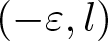 $(-\varepsilon,l)$. We have the estimates (4.28) using the above definitions and (4.29). Using the estimate (4.16) $_3$ and Poincaré inequality, we get with
 \begin{equation}
\|F^{\diamond}\|_{H^1\big(-{\delta\over 2},L+{\delta\over 2}\big)}+\|G^{\diamond}\|_{H^1\big(-{\delta\over 2},L+{\delta\over 2}\big)}\leq {C\over \varepsilon^{1/2}\delta}\textbf{D}(v).
\end{equation}
\begin{equation}
\|F^{\diamond}\|_{H^1\big(-{\delta\over 2},L+{\delta\over 2}\big)}+\|G^{\diamond}\|_{H^1\big(-{\delta\over 2},L+{\delta\over 2}\big)}\leq {C\over \varepsilon^{1/2}\delta}\textbf{D}(v).
\end{equation} We also have using (4.17) $_1$ and (4.30)
 \begin{align*}
&\|\partial_1{\mathcal{U}}^{\diamond}-d_1F^{\diamond}\|_{L^2({\omega}_\delta)}\\
&\quad\leq \|\partial_1{\mathcal{V}}^{\diamond}-\textbf{R}^\circ\textbf{e}_1\|_{L^2({\omega}_\delta)}+\|\textbf{R}^\circ\textbf{e}_1-\textbf{R}^{\diamond}(\cdot,0)\textbf{e}_1\|_{L^2({\omega}_\delta)}
\leq {C\over \varepsilon^{3/2}}\textbf{D}(v).
\end{align*}
\begin{align*}
&\|\partial_1{\mathcal{U}}^{\diamond}-d_1F^{\diamond}\|_{L^2({\omega}_\delta)}\\
&\quad\leq \|\partial_1{\mathcal{V}}^{\diamond}-\textbf{R}^\circ\textbf{e}_1\|_{L^2({\omega}_\delta)}+\|\textbf{R}^\circ\textbf{e}_1-\textbf{R}^{\diamond}(\cdot,0)\textbf{e}_1\|_{L^2({\omega}_\delta)}
\leq {C\over \varepsilon^{3/2}}\textbf{D}(v).
\end{align*}Similarly, we obtain
 \begin{equation*}\|\partial_2{\mathcal{U}}^{\diamond}-d_2G^{\diamond}\|_{L^2({\omega}_\delta)}\leq {C\over \varepsilon^{3/2}}\textbf{D}(v).\end{equation*}
The above inequalities, using Poincaré inequality, we get (4.27). This completes the proof.
4.2.2. Main decomposition result: The main fields
${\mathcal{V}}$ and
$\textbf{R}$


With the notation illustrated in Figure 2, set
 \begin{equation}
\begin{aligned}
& R^1_{pq}\,:\, (p\varepsilon,q\varepsilon)+{\mathfrak{J}}_{\varepsilon\delta}\times {\mathfrak{I}}_\delta,\qquad &&(p,q)\in {\mathcal K}^{(1)}_\varepsilon,\\
& R^2_{pq}\,:\, (p\varepsilon,q\varepsilon)+{\mathfrak{I}}_\delta\times {\mathfrak{J}}_{\varepsilon\delta},\qquad &&(p,q)\in {\mathcal K}^{(2)}_\varepsilon,\\
& R^3_{pq}\,:\, (p\varepsilon,q\varepsilon)+{\mathfrak{I}}_\delta^2,\qquad &&(p,q)\in {\mathcal K}_\varepsilon,
\end{aligned}
\end{equation}
\begin{equation}
\begin{aligned}
& R^1_{pq}\,:\, (p\varepsilon,q\varepsilon)+{\mathfrak{J}}_{\varepsilon\delta}\times {\mathfrak{I}}_\delta,\qquad &&(p,q)\in {\mathcal K}^{(1)}_\varepsilon,\\
& R^2_{pq}\,:\, (p\varepsilon,q\varepsilon)+{\mathfrak{I}}_\delta\times {\mathfrak{J}}_{\varepsilon\delta},\qquad &&(p,q)\in {\mathcal K}^{(2)}_\varepsilon,\\
& R^3_{pq}\,:\, (p\varepsilon,q\varepsilon)+{\mathfrak{I}}_\delta^2,\qquad &&(p,q)\in {\mathcal K}_\varepsilon,
\end{aligned}
\end{equation}where  ${\mathfrak{J}}_{\varepsilon\delta}=({\delta\over 2},\varepsilon-{\delta\over 2})$.
Covering a part of  $\omega_\delta$. The soft part (red in Figure 1) is divided into three parts. (a) $\widetilde{\omega}_{pq}$. (b) Part of $\omega_\delta$.
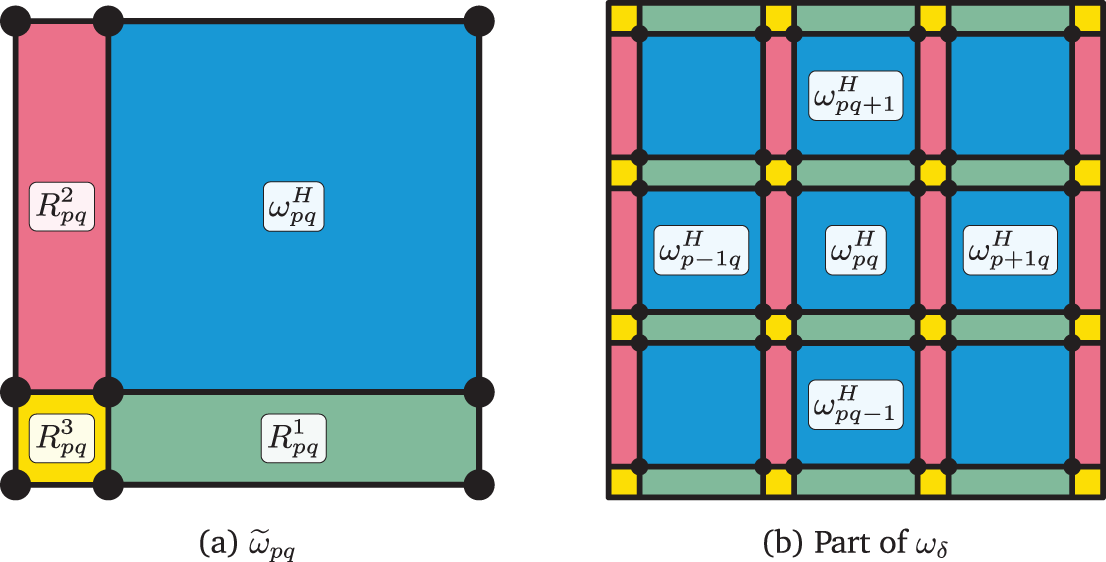
Figure 2 Long description
The image consists of two diagrams. The first diagram (a) labeled as 'tilde omega subscript p q' shows a square divided into three sections with labels: 'R superscript 2 subscript p q' on the left, 'R superscript 3 subscript p q' at the bottom left and 'R superscript 1 subscript p q' at the bottom. The center is labeled 'omega superscript H subscript p q'. The second diagram (b) labeled as 'Part of omega subscript delta' shows a grid of nine squares, each labeled with variations of 'omega superscript H' such as 'omega superscript H subscript p q plus 1', 'omega superscript H subscript p q' and 'omega superscript H subscript p q minus 1'. The grid is bordered by colored sections similar to the first diagram.
Let  $\phi_{pq}$,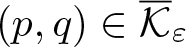 $(p,q)\in \overline{{\mathcal K}}_\varepsilon$ be real numbers. To this family of real numbers, we associate a function $\phi$ defined as follows:
 \begin{equation}
\begin{aligned}
\text{in}\ {\omega}^H_{pq}& :\phi(p\varepsilon+z_1,q\varepsilon+z_2)=\phi_{pq},\quad (z_1,z_2)\in {\mathfrak{J}}_{\varepsilon\delta}^2\\
\text{in}\ R^1_{pq}& :\phi(p\varepsilon+z_1,q\varepsilon+z_2)=\phi_{pq}{\delta+ 2z_2\over 2\delta}+\phi_{pq-1}{\delta-2z_2\over 2\delta}, \quad (z_1,z_2)\in {\mathfrak{J}}_{\varepsilon\delta}\times {\mathfrak{I}}_\delta,\\
\text{in}\ R^2_{pq}& :\phi(p\varepsilon+z_1,q\varepsilon+z_2)=\phi_{pq}{\delta+ 2z_1\over 2\delta}+\phi_{p-1q}{\delta-2z_1\over 2\delta},\quad (z_1,z_2)\in {\mathfrak{I}}_{\delta}\times {\mathfrak{J}}_{\varepsilon\delta},\\
\text{in}\ R^3_{pq}& :\phi(p\varepsilon+z_1,q\varepsilon+z_2)=\phi_{pq}{\delta+ 2z_1\over 2\delta}{\delta+ 2z_2\over 2\delta}+\phi_{pq-1}{\delta+ 2z_1\over 2\delta}{\delta-2z_2\over 2\delta}\\
& \quad+\phi_{p-1q} {\delta- 2z_1\over 2\delta}{\delta+ 2z_2\over 2\delta}+\phi_{p-1q-1}{\delta- 2z_1\over 2\delta}{\delta-2z_2\over 2\delta},\quad (z_1,z_2)\in {\mathfrak{I}}^2_{\delta}.
\end{aligned}
\end{equation}
\begin{equation}
\begin{aligned}
\text{in}\ {\omega}^H_{pq}& :\phi(p\varepsilon+z_1,q\varepsilon+z_2)=\phi_{pq},\quad (z_1,z_2)\in {\mathfrak{J}}_{\varepsilon\delta}^2\\
\text{in}\ R^1_{pq}& :\phi(p\varepsilon+z_1,q\varepsilon+z_2)=\phi_{pq}{\delta+ 2z_2\over 2\delta}+\phi_{pq-1}{\delta-2z_2\over 2\delta}, \quad (z_1,z_2)\in {\mathfrak{J}}_{\varepsilon\delta}\times {\mathfrak{I}}_\delta,\\
\text{in}\ R^2_{pq}& :\phi(p\varepsilon+z_1,q\varepsilon+z_2)=\phi_{pq}{\delta+ 2z_1\over 2\delta}+\phi_{p-1q}{\delta-2z_1\over 2\delta},\quad (z_1,z_2)\in {\mathfrak{I}}_{\delta}\times {\mathfrak{J}}_{\varepsilon\delta},\\
\text{in}\ R^3_{pq}& :\phi(p\varepsilon+z_1,q\varepsilon+z_2)=\phi_{pq}{\delta+ 2z_1\over 2\delta}{\delta+ 2z_2\over 2\delta}+\phi_{pq-1}{\delta+ 2z_1\over 2\delta}{\delta-2z_2\over 2\delta}\\
& \quad+\phi_{p-1q} {\delta- 2z_1\over 2\delta}{\delta+ 2z_2\over 2\delta}+\phi_{p-1q-1}{\delta- 2z_1\over 2\delta}{\delta-2z_2\over 2\delta},\quad (z_1,z_2)\in {\mathfrak{I}}^2_{\delta}.
\end{aligned}
\end{equation} Now, we define global fields  ${\mathcal{V}}\in H^1({\omega}_\delta)^3$ and $\textbf{R}\in H^1({\omega}_\delta)^{3\times 3}$, for that we set
 \begin{equation*}
\begin{aligned}
&\textbf{R}(p\varepsilon+z_1,q\varepsilon+z_2)=\textbf{R}_{pq},\\
&{\mathcal{V}}(p\varepsilon+z_1,q\varepsilon+z_2)=\textbf{a}_{pq}+\textbf{R}_{pq}(z_1\textbf{e}_1+z_2\textbf{e}_2),
\end{aligned}
\qquad \hbox{for all } z\in {\mathfrak{J}}_{\varepsilon\delta}^2,\quad (p,q)\in \overline{{\mathcal{K}}}_\varepsilon.
\end{equation*}
\begin{equation*}
\begin{aligned}
&\textbf{R}(p\varepsilon+z_1,q\varepsilon+z_2)=\textbf{R}_{pq},\\
&{\mathcal{V}}(p\varepsilon+z_1,q\varepsilon+z_2)=\textbf{a}_{pq}+\textbf{R}_{pq}(z_1\textbf{e}_1+z_2\textbf{e}_2),
\end{aligned}
\qquad \hbox{for all } z\in {\mathfrak{J}}_{\varepsilon\delta}^2,\quad (p,q)\in \overline{{\mathcal{K}}}_\varepsilon.
\end{equation*} The field  $\textbf{R}$ is defined from the family of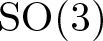 $\mathrm{SO}(3)$ matrices $\textbf{R}_{pq}$,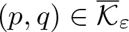 $(p,q)\in\overline{{\mathcal K}}_\varepsilon$, using (4.33). ${\mathcal{V}}$ is defined as the ${\mathcal{Q}}_1$-interpolate of its values at the vertices of the above rectangles or squares (4.32). So, these fields are defined in ${\omega}_\delta$ and from the above constructions we have $\textbf{R}\in H^1({\omega}_\delta)^{3\times 3}$ and ${\mathcal{V}}\in H^1({\omega}_\delta)^3$.
We have the following expressions of  ${\cal V}$:
 \begin{equation}
{\begin{aligned}
\hbox{in }R^1_{pq} &:{\cal V}(p\varepsilon+z_1,q\varepsilon+z_2)\\
&= \Big(\textbf{a}_{pq}+\textbf{R}_{pq}\left(\begin{matrix} \displaystyle z_1 \\ \displaystyle \delta/2 \\ 0 \end{matrix}\right)\Big){\delta+ 2z_2\over 2\delta}+\Big(\textbf{a}_{pq-1}+\textbf{R}_{pq-1}\left(\begin{matrix} \displaystyle z_1 \\ \displaystyle \varepsilon-\delta/2\\ 0 \end{matrix}\right)\Big){\delta-2z_2\over 2\delta},\\
& \quad (z_1,z_2)\in {\mathfrak{J}}_{\varepsilon\delta}\times {\mathfrak{I}}_\delta,\\
\hbox{in }R^2_{pq} &: {\cal V}(p\varepsilon+z_1,q\varepsilon+z_2)\\
&= \Big(\textbf{a}_{pq}+\textbf{R}_{pq}\left(\begin{matrix} \displaystyle \delta/2 \\ \displaystyle z_2 \\ 0 \end{matrix}\right)\Big){\delta+ 2z_1\over 2\delta}+\Big(\textbf{a}_{p-1q}+\textbf{R}_{p-1q}\left(\begin{matrix} \displaystyle \varepsilon-\delta/2 \\ \displaystyle z_2 \\ 0 \end{matrix}\right)\Big){\delta-2z_1\over 2\delta},\\
&\quad (z_1,z_2)\in {\mathfrak{I}}_{\delta}\times {\mathfrak{J}}_{\varepsilon\delta},\\
\hbox{in }R^3_{pq} & : {\cal V}(p\varepsilon+z_1,q\varepsilon+z_2)\\
&=\Big(\textbf{a}_{pq}+\textbf{R}_{pq}\left(\begin{matrix} \displaystyle \delta/2\\ \displaystyle \delta/2 \\ 0 \end{matrix}\right) \Big){\delta+ 2z_1\over 2\delta}{\delta+ 2z_2\over 2\delta}+\Big(\textbf{a}_{pq-1}+\textbf{R}_{pq-1} \left(\begin{matrix} \displaystyle \delta/2 \\ \displaystyle \varepsilon-\delta/2\\ 0 \end{matrix}\right)\Big)\\
&\quad{\delta+ 2z_1\over 2\delta}{\delta-2z_2\over 2\delta} +\Big(\textbf{a}_{p-1q}+ \textbf{R}_{p-1q} \left(\begin{matrix} \displaystyle \varepsilon -\delta/2\\ \displaystyle \delta/2 \\ 0 \end{matrix}\right) \Big){\delta- 2z_1\over 2\delta}{\delta+ 2z_2\over 2\delta}\\
&\quad +\Big(\textbf{a}_{p-1q-1}+\textbf{R}_{p-1q-1}\left(\begin{matrix} \displaystyle \varepsilon-\delta/2\\ \displaystyle \varepsilon-\delta/2 \\ 0 \end{matrix}\right) \Big){\delta- 2z_1\over 2\delta}{\delta-2z_2\over 2\delta}, \quad (z_1,z_2)\in {\mathfrak{I}}^2_{\delta}.
\end{aligned}
}
\end{equation}
\begin{equation}
{\begin{aligned}
\hbox{in }R^1_{pq} &:{\cal V}(p\varepsilon+z_1,q\varepsilon+z_2)\\
&= \Big(\textbf{a}_{pq}+\textbf{R}_{pq}\left(\begin{matrix} \displaystyle z_1 \\ \displaystyle \delta/2 \\ 0 \end{matrix}\right)\Big){\delta+ 2z_2\over 2\delta}+\Big(\textbf{a}_{pq-1}+\textbf{R}_{pq-1}\left(\begin{matrix} \displaystyle z_1 \\ \displaystyle \varepsilon-\delta/2\\ 0 \end{matrix}\right)\Big){\delta-2z_2\over 2\delta},\\
& \quad (z_1,z_2)\in {\mathfrak{J}}_{\varepsilon\delta}\times {\mathfrak{I}}_\delta,\\
\hbox{in }R^2_{pq} &: {\cal V}(p\varepsilon+z_1,q\varepsilon+z_2)\\
&= \Big(\textbf{a}_{pq}+\textbf{R}_{pq}\left(\begin{matrix} \displaystyle \delta/2 \\ \displaystyle z_2 \\ 0 \end{matrix}\right)\Big){\delta+ 2z_1\over 2\delta}+\Big(\textbf{a}_{p-1q}+\textbf{R}_{p-1q}\left(\begin{matrix} \displaystyle \varepsilon-\delta/2 \\ \displaystyle z_2 \\ 0 \end{matrix}\right)\Big){\delta-2z_1\over 2\delta},\\
&\quad (z_1,z_2)\in {\mathfrak{I}}_{\delta}\times {\mathfrak{J}}_{\varepsilon\delta},\\
\hbox{in }R^3_{pq} & : {\cal V}(p\varepsilon+z_1,q\varepsilon+z_2)\\
&=\Big(\textbf{a}_{pq}+\textbf{R}_{pq}\left(\begin{matrix} \displaystyle \delta/2\\ \displaystyle \delta/2 \\ 0 \end{matrix}\right) \Big){\delta+ 2z_1\over 2\delta}{\delta+ 2z_2\over 2\delta}+\Big(\textbf{a}_{pq-1}+\textbf{R}_{pq-1} \left(\begin{matrix} \displaystyle \delta/2 \\ \displaystyle \varepsilon-\delta/2\\ 0 \end{matrix}\right)\Big)\\
&\quad{\delta+ 2z_1\over 2\delta}{\delta-2z_2\over 2\delta} +\Big(\textbf{a}_{p-1q}+ \textbf{R}_{p-1q} \left(\begin{matrix} \displaystyle \varepsilon -\delta/2\\ \displaystyle \delta/2 \\ 0 \end{matrix}\right) \Big){\delta- 2z_1\over 2\delta}{\delta+ 2z_2\over 2\delta}\\
&\quad +\Big(\textbf{a}_{p-1q-1}+\textbf{R}_{p-1q-1}\left(\begin{matrix} \displaystyle \varepsilon-\delta/2\\ \displaystyle \varepsilon-\delta/2 \\ 0 \end{matrix}\right) \Big){\delta- 2z_1\over 2\delta}{\delta-2z_2\over 2\delta}, \quad (z_1,z_2)\in {\mathfrak{I}}^2_{\delta}.
\end{aligned}
}
\end{equation} Now, we define the residual deformation  $\overline{v}$ by
 \begin{equation}
\overline{v}=v-V_e,\qquad V_e(x)={\mathcal{V}}(x')+x_3\textbf{R}(x')\textbf{e}_3\qquad \hbox{for a.e. } x\in \Omega_\delta.
\end{equation}
\begin{equation}
\overline{v}=v-V_e,\qquad V_e(x)={\mathcal{V}}(x')+x_3\textbf{R}(x')\textbf{e}_3\qquad \hbox{for a.e. } x\in \Omega_\delta.
\end{equation}Observe that
 \begin{equation*}
\overline{v}=0,\quad\text{a.e. in}\ \Omega^H_{pq},\quad\text{and}\quad \partial_\alpha{\mathcal{V}}-\textbf{R}\textbf{e}_\alpha=0\quad\text{a.e. in}\ {\omega}^H_{pq}\hbox{for all } (p,q)\in {\mathcal{K}}_\varepsilon^*.
\end{equation*}
\begin{equation*}
\overline{v}=0,\quad\text{a.e. in}\ \Omega^H_{pq},\quad\text{and}\quad \partial_\alpha{\mathcal{V}}-\textbf{R}\textbf{e}_\alpha=0\quad\text{a.e. in}\ {\omega}^H_{pq}\hbox{for all } (p,q)\in {\mathcal{K}}_\varepsilon^*.
\end{equation*} Due to the  ${\mathcal{Q}}_1$-nature of the fields ${\mathcal{V}}$ and $\textbf{R}$, we have
 \begin{equation}
V_e=I_d\qquad \hbox{a.e. in }\Gamma_\delta.
\end{equation}
\begin{equation}
V_e=I_d\qquad \hbox{a.e. in }\Gamma_\delta.
\end{equation}In the lemma below, we give estimates for all these fields.
Lemma 4.9. We have
 \begin{align}
& \|\nabla \mathbf{R}\|_{L^2({\omega}_\delta)} \leq {C\over \delta^{3/2}}\mathbf{D}(v),\quad \|\partial_\alpha\mathbf{R}\mathbf{e}_{3-\alpha}\|_{L^2({\omega}_\delta)}\leq {C\over \varepsilon\delta^{1/2}}\mathbf{D}(v),\nonumber\\
&\|\mathbf{R}-\mathbf{I}_3\|_{L^2({\omega}_\delta)}\leq {C\over \varepsilon^{1/2}\delta}\mathbf{D}(v),\nonumber\\
&\|\mathbf{R}-\mathbf{R}^\diamond\|_{L^2({\omega}_\delta)}\leq C{\varepsilon^{1/2}\over\delta}\mathbf{D}(v),\qquad \|\mathbf{R}-\mathbf{R}^\circ\|_{L^2({\omega}_\delta)}\leq {C\over\delta^{1/2}}\mathbf{D}(v),
\end{align}
\begin{align}
& \|\nabla \mathbf{R}\|_{L^2({\omega}_\delta)} \leq {C\over \delta^{3/2}}\mathbf{D}(v),\quad \|\partial_\alpha\mathbf{R}\mathbf{e}_{3-\alpha}\|_{L^2({\omega}_\delta)}\leq {C\over \varepsilon\delta^{1/2}}\mathbf{D}(v),\nonumber\\
&\|\mathbf{R}-\mathbf{I}_3\|_{L^2({\omega}_\delta)}\leq {C\over \varepsilon^{1/2}\delta}\mathbf{D}(v),\nonumber\\
&\|\mathbf{R}-\mathbf{R}^\diamond\|_{L^2({\omega}_\delta)}\leq C{\varepsilon^{1/2}\over\delta}\mathbf{D}(v),\qquad \|\mathbf{R}-\mathbf{R}^\circ\|_{L^2({\omega}_\delta)}\leq {C\over\delta^{1/2}}\mathbf{D}(v),
\end{align}and
 \begin{equation}
\begin{aligned}
&\|\partial_\alpha{\mathcal{V}}-\mathbf{R}\mathbf{e}_\alpha\|_{L^2({\omega}_\delta)}\leq {C\over \delta^{1/2}}\mathbf{D}(v),\quad \|{\mathcal{V}}-I_d\|_{H^1({\omega}_\delta)}\leq {C\over \varepsilon^{1/2}\delta}\mathbf{D}(v),\\
&\|\overline{v}\|_{L^2(\Omega_\delta)}\leq C\delta\mathbf{D}(v),\qquad \|\nabla \overline{v}\|_{L^2(\Omega_\delta)} + \|\nabla v-\mathbf{R}\|_{L^2(\Omega_\delta)} \leq C\mathbf{D}(v).
\end{aligned}
\end{equation}
\begin{equation}
\begin{aligned}
&\|\partial_\alpha{\mathcal{V}}-\mathbf{R}\mathbf{e}_\alpha\|_{L^2({\omega}_\delta)}\leq {C\over \delta^{1/2}}\mathbf{D}(v),\quad \|{\mathcal{V}}-I_d\|_{H^1({\omega}_\delta)}\leq {C\over \varepsilon^{1/2}\delta}\mathbf{D}(v),\\
&\|\overline{v}\|_{L^2(\Omega_\delta)}\leq C\delta\mathbf{D}(v),\qquad \|\nabla \overline{v}\|_{L^2(\Omega_\delta)} + \|\nabla v-\mathbf{R}\|_{L^2(\Omega_\delta)} \leq C\mathbf{D}(v).
\end{aligned}
\end{equation}Moreover, we have
 \begin{equation}
\left\|\mathfrak{R}-\mathbf{R}\right\|_{L^2({\omega}_\delta)}+\|\nabla(\mathfrak{V}-{\mathcal{V}})\|_{L^2({\omega}_\delta)}\leq {C\over \delta^{1/2}}\mathbf{D}(v),
\end{equation}
\begin{equation}
\left\|\mathfrak{R}-\mathbf{R}\right\|_{L^2({\omega}_\delta)}+\|\nabla(\mathfrak{V}-{\mathcal{V}})\|_{L^2({\omega}_\delta)}\leq {C\over \delta^{1/2}}\mathbf{D}(v),
\end{equation} \begin{equation}
\|\mathfrak{V}-{\mathcal{V}}\|_{L^2({\omega}_\delta)}\leq C\delta^{1/2}\mathbf{D}(v).
\end{equation}
\begin{equation}
\|\mathfrak{V}-{\mathcal{V}}\|_{L^2({\omega}_\delta)}\leq C\delta^{1/2}\mathbf{D}(v).
\end{equation} The constants do not depend on  $\varepsilon$ and $\delta$.
Proof. Step 1. We prove (4.37).
In the rectangles  $R^2_{pq}$ for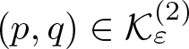 $(p,q)\in{\mathcal{K}}_\varepsilon^{(2)}$, we have
 \begin{equation}
\begin{aligned}
{\partial}_1\textbf{R}(p\varepsilon+z_1,q\varepsilon+z_2)=&{1\over \delta}( \textbf{R}_{pq}-\textbf{R}_{p-1q}),\quad\forall\,(z_1,z_2)\in{\mathfrak{I}}_\delta\times {\mathfrak{J}}_{\varepsilon\delta}.
\end{aligned}
\end{equation}
\begin{equation}
\begin{aligned}
{\partial}_1\textbf{R}(p\varepsilon+z_1,q\varepsilon+z_2)=&{1\over \delta}( \textbf{R}_{pq}-\textbf{R}_{p-1q}),\quad\forall\,(z_1,z_2)\in{\mathfrak{I}}_\delta\times {\mathfrak{J}}_{\varepsilon\delta}.
\end{aligned}
\end{equation}So, we have
 \begin{align}
& \|\partial_1\textbf{R}\|^2_{L^2(R^2_{pq})}\leq {C\varepsilon\over \delta}|\textbf{R}_{pq}-\textbf{R}_{p-1q}|^2\quad \hbox{and}\nonumber\\
& \|\partial_1\textbf{R}\textbf{e}_2\|^2_{L^2(R^2_{pq})}\leq {C\varepsilon\over \delta}|(\textbf{R}_{pq}-\textbf{R}_{p-1q})\textbf{e}_2|^2.
\end{align}
\begin{align}
& \|\partial_1\textbf{R}\|^2_{L^2(R^2_{pq})}\leq {C\varepsilon\over \delta}|\textbf{R}_{pq}-\textbf{R}_{p-1q}|^2\quad \hbox{and}\nonumber\\
& \|\partial_1\textbf{R}\textbf{e}_2\|^2_{L^2(R^2_{pq})}\leq {C\varepsilon\over \delta}|(\textbf{R}_{pq}-\textbf{R}_{p-1q})\textbf{e}_2|^2.
\end{align} Similarly, in the rectangles  $R^1_{pq}$ for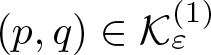 $(p,q)\in{\mathcal{K}}_\varepsilon^{(1)}$, we have
 \begin{align}
& \|\partial_2\textbf{R}\|^2_{L^2(R^1_{pq})}\leq {C\varepsilon\over \delta}|\textbf{R}_{pq}-\textbf{R}_{pq-1}|^2\quad \hbox{and}\nonumber\\
& \|\partial_2\textbf{R}\textbf{e}_1\|^2_{L^2(R^1_{pq})}\leq {C\varepsilon\over \delta}|(\textbf{R}_{pq}-\textbf{R}_{pq-1})\textbf{e}_2|^2.
\end{align}
\begin{align}
& \|\partial_2\textbf{R}\|^2_{L^2(R^1_{pq})}\leq {C\varepsilon\over \delta}|\textbf{R}_{pq}-\textbf{R}_{pq-1}|^2\quad \hbox{and}\nonumber\\
& \|\partial_2\textbf{R}\textbf{e}_1\|^2_{L^2(R^1_{pq})}\leq {C\varepsilon\over \delta}|(\textbf{R}_{pq}-\textbf{R}_{pq-1})\textbf{e}_2|^2.
\end{align} In the squares  $R^3_{pq}$ for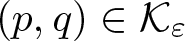 $(p,q)\in{\mathcal{K}}_\varepsilon$, we have for all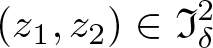 $\displaystyle(z_1,z_2)\in{\mathfrak{I}}^2_\delta$
 \begin{equation}
\begin{aligned}
{\partial}_2\textbf{R}(p\varepsilon+z_1,q\varepsilon+z_2)=&{1\over \delta}(\textbf{R}_{p-1q-1}-\textbf{R}_{p-1q-1}){{\delta}-2z_1\over 2\delta}+{1\over \delta}(\textbf{R}_{pq}-\textbf{R}_{pq-1}){{\delta}+2z_1\over 2\delta}.
\end{aligned}
\end{equation}
\begin{equation}
\begin{aligned}
{\partial}_2\textbf{R}(p\varepsilon+z_1,q\varepsilon+z_2)=&{1\over \delta}(\textbf{R}_{p-1q-1}-\textbf{R}_{p-1q-1}){{\delta}-2z_1\over 2\delta}+{1\over \delta}(\textbf{R}_{pq}-\textbf{R}_{pq-1}){{\delta}+2z_1\over 2\delta}.
\end{aligned}
\end{equation} Similarly, we compute  ${\partial}_2\textbf{R}$. So, we have
 \begin{equation}
\begin{aligned}
&\|\partial_1\textbf{R}\|^2_{L^2(R^3_{pq})}\leq C\big(|\textbf{R}_{pq-1}-\textbf{R}_{p-1q-1}|^2+|\textbf{R}_{pq}-\textbf{R}_{p-1q}|^2\Big),\\
&\|\partial_1\textbf{R}\textbf{e}_2\|^2_{L^2(R^3_{pq})}\leq C\big(|(\textbf{R}_{pq-1}-\textbf{R}_{p-1q-1})\textbf{e}_2|^2+|(\textbf{R}_{pq}-\textbf{R}_{p-1q})\textbf{e}_2|^2\Big),\\
\hbox{and}\;\; \;
&\|\partial_2\textbf{R}\|^2_{L^2(R^3_{pq})}\leq C\big(|\textbf{R}_{p-1q}-\textbf{R}_{p-1q-1}|^2+|\textbf{R}_{pq}-\textbf{R}_{pq-1}|^2\big), \\
&\|\partial_2\textbf{R}\textbf{e}_1\|^2_{L^2(R^3_{pq})}\leq C\big(|(\textbf{R}_{p-1q}-\textbf{R}_{p-1q-1})\textbf{e}_1|^2+|(\textbf{R}_{pq}-\textbf{R}_{pq-1})\textbf{e}_1|^2\big).
\end{aligned}
\end{equation}
\begin{equation}
\begin{aligned}
&\|\partial_1\textbf{R}\|^2_{L^2(R^3_{pq})}\leq C\big(|\textbf{R}_{pq-1}-\textbf{R}_{p-1q-1}|^2+|\textbf{R}_{pq}-\textbf{R}_{p-1q}|^2\Big),\\
&\|\partial_1\textbf{R}\textbf{e}_2\|^2_{L^2(R^3_{pq})}\leq C\big(|(\textbf{R}_{pq-1}-\textbf{R}_{p-1q-1})\textbf{e}_2|^2+|(\textbf{R}_{pq}-\textbf{R}_{p-1q})\textbf{e}_2|^2\Big),\\
\hbox{and}\;\; \;
&\|\partial_2\textbf{R}\|^2_{L^2(R^3_{pq})}\leq C\big(|\textbf{R}_{p-1q}-\textbf{R}_{p-1q-1}|^2+|\textbf{R}_{pq}-\textbf{R}_{pq-1}|^2\big), \\
&\|\partial_2\textbf{R}\textbf{e}_1\|^2_{L^2(R^3_{pq})}\leq C\big(|(\textbf{R}_{p-1q}-\textbf{R}_{p-1q-1})\textbf{e}_1|^2+|(\textbf{R}_{pq}-\textbf{R}_{pq-1})\textbf{e}_1|^2\big).
\end{aligned}
\end{equation}Then, using the above results, we get
 \begin{align*}
&\|\nabla \textbf{R}\|^2_{L^2({\omega}_\delta)}\leq {C\varepsilon\over \delta}\Big(\sum_{p=0}^{N_\varepsilon}\sum_{q=0}^{N_\varepsilon-1}|\textbf{R}_{pq}-\textbf{R}_{p-1q}|^2+ \sum_{q=0}^{N_\varepsilon}\sum_{p=0}^{N_\varepsilon-1}|\textbf{R}_{pq}-\textbf{R}_{pq-1}|^2\Big),\\
&\|\partial_1 \textbf{R}\textbf{e}_2\|^2_{L^2({\omega}_\delta)}\leq {C\varepsilon\over \delta}\sum_{p=0}^{N_\varepsilon}\sum_{q=0}^{N_\varepsilon-1}|(\textbf{R}_{pq}-\textbf{R}_{p-1q})\textbf{e}_2|^2,\\
& \|\partial_2 \textbf{R}\textbf{e}_1\|^2_{L^2({\omega}_\delta)}\leq {C\varepsilon\over \delta}\sum_{q=0}^{N_\varepsilon}\sum_{p=0}^{N_\varepsilon-1}|(\textbf{R}_{pq}-\textbf{R}_{pq-1})\textbf{e}_1|^2.
\end{align*}
\begin{align*}
&\|\nabla \textbf{R}\|^2_{L^2({\omega}_\delta)}\leq {C\varepsilon\over \delta}\Big(\sum_{p=0}^{N_\varepsilon}\sum_{q=0}^{N_\varepsilon-1}|\textbf{R}_{pq}-\textbf{R}_{p-1q}|^2+ \sum_{q=0}^{N_\varepsilon}\sum_{p=0}^{N_\varepsilon-1}|\textbf{R}_{pq}-\textbf{R}_{pq-1}|^2\Big),\\
&\|\partial_1 \textbf{R}\textbf{e}_2\|^2_{L^2({\omega}_\delta)}\leq {C\varepsilon\over \delta}\sum_{p=0}^{N_\varepsilon}\sum_{q=0}^{N_\varepsilon-1}|(\textbf{R}_{pq}-\textbf{R}_{p-1q})\textbf{e}_2|^2,\\
& \|\partial_2 \textbf{R}\textbf{e}_1\|^2_{L^2({\omega}_\delta)}\leq {C\varepsilon\over \delta}\sum_{q=0}^{N_\varepsilon}\sum_{p=0}^{N_\varepsilon-1}|(\textbf{R}_{pq}-\textbf{R}_{pq-1})\textbf{e}_1|^2.
\end{align*} Then, the estimates (4.11) $_{1,2,3,4}$ and the above inequalities with (4.42) $_2$, (4.43) $_2$, (4.45) $_{2,4}$ give (4.37) $_{1,2}$. The estimate (4.37) $_{3}$ is a consequence of (4.16) $_{2,4}$.
Besides, since  $\textbf{R}$ is constant and equal to $\textbf{R}_{pq}$ in ${\omega}^H_{pq}$, due to (4.9) and (4.37) $_1$, we have
 \begin{equation}
\sum_{(p,q)\in {\mathcal{K}}^*_\varepsilon}\big\|\textbf{R}-\textbf{R}_{pq}\big\|^2_{L^2(\widetilde {\omega}_{pq})}\leq C\delta^2 \|\nabla \textbf{R}\|^2_{L^2({\omega}_\delta)}\leq {C\over \delta}\textbf{D}(v)^2.
\end{equation}
\begin{equation}
\sum_{(p,q)\in {\mathcal{K}}^*_\varepsilon}\big\|\textbf{R}-\textbf{R}_{pq}\big\|^2_{L^2(\widetilde {\omega}_{pq})}\leq C\delta^2 \|\nabla \textbf{R}\|^2_{L^2({\omega}_\delta)}\leq {C\over \delta}\textbf{D}(v)^2.
\end{equation} The estimates (4.23) and (4.46) give (4.37) $_4$. The above estimate (4.46) also implies (4.37) $_5$.
$_5$.
Step 2. We prove (4.38) $_{1,2}$.
Using the definition of  ${\mathcal{V}}$ and $\textbf{R}$, we have $\partial_1{\mathcal{V}}-\textbf{R}\textbf{e}_1$ vanishes in ${\omega}^H_{pq}$ for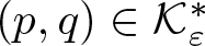 $(p,q)\in{\mathcal{K}}_\varepsilon^*$ and in rectangle $R^1_{pq}$ for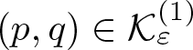 $(p,q)\in {\mathcal{K}}_\varepsilon^{(1)}$. In $R^2_{pq}$ for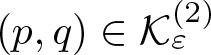 $(p,q)\in{\mathcal{K}}_\varepsilon^{(2)}$ we have
 \begin{equation}
\begin{aligned}
\big(\partial_1{\mathcal{V}}-\textbf{R}\textbf{e}_1\big)(p\varepsilon+z_1,q\varepsilon+z_2)&={1\over \delta}\big(\textbf{a}_{pq}-\textbf{a}_{p-1q}- \varepsilon\textbf{R}_{p-1q}\textbf{e}_1\big)\\
&\hskip -25mm +{z_2\over \delta}(\textbf{R}_{pq}-\textbf{R}_{p-1q})\textbf{e}_2
-{z_1\over \delta}(\textbf{R}_{pq}-\textbf{R}_{p-1q})\textbf{e}_1,\quad (z_1,z_2)\in {\mathfrak{I}}_\delta\times {\mathfrak{J}}_{\varepsilon\delta},
\end{aligned}
\end{equation}
\begin{equation}
\begin{aligned}
\big(\partial_1{\mathcal{V}}-\textbf{R}\textbf{e}_1\big)(p\varepsilon+z_1,q\varepsilon+z_2)&={1\over \delta}\big(\textbf{a}_{pq}-\textbf{a}_{p-1q}- \varepsilon\textbf{R}_{p-1q}\textbf{e}_1\big)\\
&\hskip -25mm +{z_2\over \delta}(\textbf{R}_{pq}-\textbf{R}_{p-1q})\textbf{e}_2
-{z_1\over \delta}(\textbf{R}_{pq}-\textbf{R}_{p-1q})\textbf{e}_1,\quad (z_1,z_2)\in {\mathfrak{I}}_\delta\times {\mathfrak{J}}_{\varepsilon\delta},
\end{aligned}
\end{equation}which along with (4.11) $_{1,3,5}$ imply
 \begin{equation}
\sum_{q=0}^{N_\varepsilon-1}\sum_{p=0}^{N_\varepsilon}\|\partial_1{\mathcal{V}}-\textbf{R}\textbf{e}_1\|^2_{L^2(R^2_{pq})}\leq{C\over \delta}\textbf{D}(v)^2.
\end{equation}
\begin{equation}
\sum_{q=0}^{N_\varepsilon-1}\sum_{p=0}^{N_\varepsilon}\|\partial_1{\mathcal{V}}-\textbf{R}\textbf{e}_1\|^2_{L^2(R^2_{pq})}\leq{C\over \delta}\textbf{D}(v)^2.
\end{equation} In the square  $R^3_{pq}$, from (4.47), we have
 \begin{equation*}
\begin{aligned}
& \big(\partial_1{\cal V}-\textbf{R} \textbf{e}_1\big)(p\varepsilon+z_1,q\varepsilon+z_2)\\
& \quad={1\over \delta}\Big(\Big(\textbf{a}_{pq}-\textbf{a}_{p-1q} - \varepsilon\textbf{R}_{p-1q}\textbf{e}_1\Big) - z_1(\textbf{R}_{pq}-\textbf{R}_{p-1q}) \textbf{e}_1\Big){\delta+2z_2\over 2\delta}\\
&\qquad+{1\over \delta}\Big(\Big(\textbf{a}_{pq-1}-\textbf{a}_{p-1q-1} -\varepsilon\textbf{R}_{p-1q-1}\textbf{e}_1\Big) - z_1(\textbf{R}_{pq-1}-\textbf{R}_{p-1q-1})\textbf{e}_1\Big){\delta-2z_2\over 2\delta}\\
&\qquad+{\delta+2z_2\over 2\delta}(\textbf{R}_{pq}-\textbf{R}_{p-1q})\textbf{e}_2+{\delta-2z_2\over 2\delta}(\textbf{R}_{pq-1}-\textbf{R}_{p-1q-1})\textbf{e}_2,\qquad (z_1,z_2)\in {\mathfrak{I}}_\delta^2,
\end{aligned}
\end{equation*}
\begin{equation*}
\begin{aligned}
& \big(\partial_1{\cal V}-\textbf{R} \textbf{e}_1\big)(p\varepsilon+z_1,q\varepsilon+z_2)\\
& \quad={1\over \delta}\Big(\Big(\textbf{a}_{pq}-\textbf{a}_{p-1q} - \varepsilon\textbf{R}_{p-1q}\textbf{e}_1\Big) - z_1(\textbf{R}_{pq}-\textbf{R}_{p-1q}) \textbf{e}_1\Big){\delta+2z_2\over 2\delta}\\
&\qquad+{1\over \delta}\Big(\Big(\textbf{a}_{pq-1}-\textbf{a}_{p-1q-1} -\varepsilon\textbf{R}_{p-1q-1}\textbf{e}_1\Big) - z_1(\textbf{R}_{pq-1}-\textbf{R}_{p-1q-1})\textbf{e}_1\Big){\delta-2z_2\over 2\delta}\\
&\qquad+{\delta+2z_2\over 2\delta}(\textbf{R}_{pq}-\textbf{R}_{p-1q})\textbf{e}_2+{\delta-2z_2\over 2\delta}(\textbf{R}_{pq-1}-\textbf{R}_{p-1q-1})\textbf{e}_2,\qquad (z_1,z_2)\in {\mathfrak{I}}_\delta^2,
\end{aligned}
\end{equation*}which, along with (4.11) $_{1,5}$, gives
 \begin{equation*}
\sum_{q=0}^{N_\varepsilon}\sum_{p=0}^{N_\varepsilon}\|\partial_1{\mathcal{V}}-\textbf{R}\textbf{e}_1\|^2_{L^2(R^3_{pq})}\leq{C\over \varepsilon}\textbf{D}(v)^2.
\end{equation*}
\begin{equation*}
\sum_{q=0}^{N_\varepsilon}\sum_{p=0}^{N_\varepsilon}\|\partial_1{\mathcal{V}}-\textbf{R}\textbf{e}_1\|^2_{L^2(R^3_{pq})}\leq{C\over \varepsilon}\textbf{D}(v)^2.
\end{equation*} Then, the above and (4.48) lead to (4.38) $_{1}$ for $\alpha=1$. The case $\alpha=2$ is similar.
The estimate (4.38) $_2$ is a direct consequence of (4.37) $_3$, (4.38) $_1$, and Poincaré inequality.
Step 3. We prove (4.38) $_{3,4,5}$.
Proceeding as in Step 1 (using (4.9)) along with the definition of  $\textbf{R}$ and ${\mathcal{V}}$ along with the inequalities (4.7) $_{1,2}$, (4.5) $_{4,5}$, and (4.38) $_1$, we get (4.39).
Let us set
 \begin{equation*}{\mathcal{V}}_{pq}(x')=\textbf{a}_{pq}+\textbf{R}_{pq}\overline{x}'_{pq},\quad \text{a.e. in}\ \widetilde {\omega}_{pq}\ \text{and for}\ (p,q)\in{\mathcal{K}}_\varepsilon^*.\end{equation*}
 Since 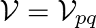 ${\mathcal{V}}={\mathcal{V}}_{pq}$ a.e. in ${\omega}^H_{pq}$, due to (4.9), for any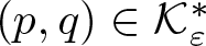 $(p,q)\in{\mathcal{K}}_\varepsilon^*$ we obtain
 \begin{equation*}\begin{aligned}
\sum_{(p,q)\in{\mathcal{K}}_\varepsilon^*}\|{\mathcal{V}} - {\mathcal{V}}_{pq}\|^2_{L^2(\widetilde {{\omega}}_{pq})} \leq C\delta^2\sum_{(p,q)\in{\mathcal{K}}_\varepsilon^*}\sum_{\alpha=1}^2\big\|\partial_\alpha{\mathcal{V}}-\textbf{R}_{pq}\textbf{e}_\alpha\big\|^2_{L^2(\widetilde {\omega}_{pq})}\\
\leq C\big(\delta^2\sum_{{\alpha}=1}^2\big\|\partial_\alpha{\mathcal{V}}-\textbf{R}\textbf{e}_\alpha\big\|^2_{L^2({\omega}_\delta)}+ \sum_{(p,q)\in{\mathcal{K}}_\varepsilon^*}\delta^2\sum_{\alpha=1}^2\big\|(\textbf{R}-\textbf{R}_{pq})\textbf{e}_\alpha\big\|^2_{L^2(\widetilde {\omega}_{pq})}\big)
\end{aligned}
\end{equation*}
\begin{equation*}\begin{aligned}
\sum_{(p,q)\in{\mathcal{K}}_\varepsilon^*}\|{\mathcal{V}} - {\mathcal{V}}_{pq}\|^2_{L^2(\widetilde {{\omega}}_{pq})} \leq C\delta^2\sum_{(p,q)\in{\mathcal{K}}_\varepsilon^*}\sum_{\alpha=1}^2\big\|\partial_\alpha{\mathcal{V}}-\textbf{R}_{pq}\textbf{e}_\alpha\big\|^2_{L^2(\widetilde {\omega}_{pq})}\\
\leq C\big(\delta^2\sum_{{\alpha}=1}^2\big\|\partial_\alpha{\mathcal{V}}-\textbf{R}\textbf{e}_\alpha\big\|^2_{L^2({\omega}_\delta)}+ \sum_{(p,q)\in{\mathcal{K}}_\varepsilon^*}\delta^2\sum_{\alpha=1}^2\big\|(\textbf{R}-\textbf{R}_{pq})\textbf{e}_\alpha\big\|^2_{L^2(\widetilde {\omega}_{pq})}\big)
\end{aligned}
\end{equation*}which, using (4.38) $_1$ and (4.46), gives
 \begin{equation*}\sum_{(p,q)\in{\mathcal{K}}_\varepsilon^*}\|{\mathcal{V}} - {\mathcal{V}}_{pq}\|^2_{L^2(\widetilde {{\omega}}_{pq})}\leq C\delta\textbf{D}(v)^2.\end{equation*}
Then, the above inequalities, along with the estimate (4.8), give
 \begin{equation*}
\|\mathfrak{V}-{\mathcal{V}}\|^2_{L^2({\omega}_\delta)}\leq 2\sum_{(p,q)\in{\mathcal{K}}_\varepsilon^*}\left(\|\mathfrak{V} - {\mathcal{V}}_{pq}\|^2_{L^2(\widetilde {{\omega}}_{pq})}+\|{\mathcal{V}} - {\mathcal{V}}_{pq}\|^2_{L^2(\widetilde {{\omega}}_{pq})}\right)\leq {C \delta}\textbf{D}(v)^2.
\end{equation*}
\begin{equation*}
\|\mathfrak{V}-{\mathcal{V}}\|^2_{L^2({\omega}_\delta)}\leq 2\sum_{(p,q)\in{\mathcal{K}}_\varepsilon^*}\left(\|\mathfrak{V} - {\mathcal{V}}_{pq}\|^2_{L^2(\widetilde {{\omega}}_{pq})}+\|{\mathcal{V}} - {\mathcal{V}}_{pq}\|^2_{L^2(\widetilde {{\omega}}_{pq})}\right)\leq {C \delta}\textbf{D}(v)^2.
\end{equation*}As a consequence of (4.39)–(4.40), we get
 \begin{equation*}\|V_e-\mathfrak{V}-x_3\mathfrak{R}\textbf{e}_3\|_{L^2(\Omega_\delta)}+\delta\|\nabla(V_e-\mathfrak{V}-x_3\mathfrak{R}\textbf{e}_3)\|_{L^2(\Omega_\delta)}\leq C\delta\textbf{D}(v).\end{equation*}
Then, we have
 \begin{equation*}\|\overline{v}\|_{L^2(\Omega_\delta)}\leq \|\overline{\mathfrak{v}}\|_{L^2(\Omega_\delta)}+\|V_e-\mathfrak{V}-x_3\mathfrak{R}\textbf{e}_3\|_{L^2(\Omega_\delta)}\leq C\delta\textbf{D}(v).\end{equation*}
 Similarly, we obtain (4.38) $_{4}$. Observe that the estimate (4.38) $_{5}$ is a consequence of (4.7) $_{1,2}$ and the definition of $\textbf{R}$. This completes the proof.
Lemma 4.10. We have
 \begin{equation}
\|\mathbf{R}(\mathbf{R})^T-\mathbf{I}_3\|_{L^2({\omega}_\delta)}\leq {C\over \delta^{1/2}}\mathbf{D}(v).
\end{equation}
\begin{equation}
\|\mathbf{R}(\mathbf{R})^T-\mathbf{I}_3\|_{L^2({\omega}_\delta)}\leq {C\over \delta^{1/2}}\mathbf{D}(v).
\end{equation}Moreover
 \begin{equation}
\|(\mathbf{R})^T+\mathbf{R}-2\mathbf{I}_3\|_{L^2({\omega}_\delta)} \leq {C\over \delta^{1/2}}\mathbf{D}(v)\big(1+{\mathbf{D}(v)\over \varepsilon\delta^{3/2}}\big).
\end{equation}
\begin{equation}
\|(\mathbf{R})^T+\mathbf{R}-2\mathbf{I}_3\|_{L^2({\omega}_\delta)} \leq {C\over \delta^{1/2}}\mathbf{D}(v)\big(1+{\mathbf{D}(v)\over \varepsilon\delta^{3/2}}\big).
\end{equation}Furthermore, the linearized strain tensor satisfies the following:
 \begin{equation}
\|(\nabla v)^T+\nabla v-2\mathbf{I}_3\|_{L^2(\Omega_\delta)}\leq C\mathbf{D}(v)\Big(1+{\mathbf{D}(v)\over \varepsilon\delta^{3/2}}\Big)
\end{equation}
\begin{equation}
\|(\nabla v)^T+\nabla v-2\mathbf{I}_3\|_{L^2(\Omega_\delta)}\leq C\mathbf{D}(v)\Big(1+{\mathbf{D}(v)\over \varepsilon\delta^{3/2}}\Big)
\end{equation} The constant(s) do not depend on  $\varepsilon$ and $\delta$.
Proof. Step 1. We prove
 \begin{equation}
\|\textbf{R}-\textbf{I}_3\|_{L^4({\omega}_\delta)}\leq C\Big(\|\textbf{R}-\textbf{I}_3\|_{L^2({\omega}_\delta)}+\sqrt{\delta\over \varepsilon}\|\nabla\textbf{R}\|_{L^2({\omega}_\delta)}\Big).
\end{equation}
\begin{equation}
\|\textbf{R}-\textbf{I}_3\|_{L^4({\omega}_\delta)}\leq C\Big(\|\textbf{R}-\textbf{I}_3\|_{L^2({\omega}_\delta)}+\sqrt{\delta\over \varepsilon}\|\nabla\textbf{R}\|_{L^2({\omega}_\delta)}\Big).
\end{equation} Due to the definitions of the functions  $\textbf{R}^\diamond$ and $\textbf{R}$ (see (4.41)–(4.45) and (4.20)), in every small square isometric to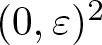 $(0,\varepsilon)^2$ and contained in ${\omega}_\delta$, these functions depend only on a finite number (independent of $\varepsilon$ and $\delta$) of matrices of the type $\textbf{R}_{pq}$. Therefore, after a straightforward calculation, we obtain that there exist two strictly positive constants $c$ and $C$, independent of $\varepsilon$ and $\delta$, such that
 \begin{equation}
\begin{aligned}
& c\|\textbf{R}^\diamond-\textbf{I}_3\|_{L^k({\omega}_\delta)}\leq \|\textbf{R}-\textbf{I}_3\|_{L^k( {\omega}_\delta)}\leq C\|\textbf{R}^\diamond-\textbf{I}_3\|_{L^k({\omega}_\delta)},\quad\text{for}\ k=2,4,\\
& \|\nabla \textbf{R}^\diamond\|_{L^2({\omega}_\delta)}\leq C\sqrt{\delta\over \varepsilon} \|\nabla \textbf{R}\|_{L^2({\omega}_\delta)}.
\end{aligned}
\end{equation}
\begin{equation}
\begin{aligned}
& c\|\textbf{R}^\diamond-\textbf{I}_3\|_{L^k({\omega}_\delta)}\leq \|\textbf{R}-\textbf{I}_3\|_{L^k( {\omega}_\delta)}\leq C\|\textbf{R}^\diamond-\textbf{I}_3\|_{L^k({\omega}_\delta)},\quad\text{for}\ k=2,4,\\
& \|\nabla \textbf{R}^\diamond\|_{L^2({\omega}_\delta)}\leq C\sqrt{\delta\over \varepsilon} \|\nabla \textbf{R}\|_{L^2({\omega}_\delta)}.
\end{aligned}
\end{equation}The above inequalities combined with (4.15) give (4.52).
Step 2. Observe that
 \begin{align}
(\textbf{R})^T\textbf{R}-\textbf{I}_3 & =(\textbf{R})^T\textbf{R}-(\textbf{R}_{pq})^T\textbf{R}_{pq}\nonumber\\
& =(\textbf{R})^T(\textbf{R}-\textbf{R}_{pq})+(\textbf{R}-\textbf{R}_{pq})^T\textbf{R}_{pq}.
\end{align}
\begin{align}
(\textbf{R})^T\textbf{R}-\textbf{I}_3 & =(\textbf{R})^T\textbf{R}-(\textbf{R}_{pq})^T\textbf{R}_{pq}\nonumber\\
& =(\textbf{R})^T(\textbf{R}-\textbf{R}_{pq})+(\textbf{R}-\textbf{R}_{pq})^T\textbf{R}_{pq}.
\end{align} Then, from (4.7) $_2$, (4.46), and the above equality, we obtain (4.49). Since the matrices $\textbf{R}_{pq}$ belong to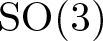 $\mathrm{SO}(3)$, the function $\textbf{R}$ is uniformly bounded and satisfies
 \begin{equation*}\|\textbf{R}\|_{L^\infty({\omega}_\delta)}\leq \sqrt{3}.\end{equation*}
We have the identities
 \begin{equation}
\begin{aligned}
&(\textbf{R})^T+\textbf{R}-2\textbf{I}_3\\
&\quad=\textbf{R}\textbf{R}(\textbf{R})^T+(\textbf{R})^T-2\textbf{R}(\textbf{R})^T+\textbf{R}(\textbf{I}_3-\textbf{R}(\textbf{R})^T)+2(\textbf{R}(\textbf{R})^T-\textbf{I}_3)\\
&\quad=(\textbf{R}-\textbf{I}_3)^2(\textbf{R})^T+\textbf{R}(\textbf{I}_3-\textbf{R}(\textbf{R})^T)+2(\textbf{R}(\textbf{R})^T)-\textbf{I}_3).
\end{aligned}
\end{equation}
\begin{equation}
\begin{aligned}
&(\textbf{R})^T+\textbf{R}-2\textbf{I}_3\\
&\quad=\textbf{R}\textbf{R}(\textbf{R})^T+(\textbf{R})^T-2\textbf{R}(\textbf{R})^T+\textbf{R}(\textbf{I}_3-\textbf{R}(\textbf{R})^T)+2(\textbf{R}(\textbf{R})^T-\textbf{I}_3)\\
&\quad=(\textbf{R}-\textbf{I}_3)^2(\textbf{R})^T+\textbf{R}(\textbf{I}_3-\textbf{R}(\textbf{R})^T)+2(\textbf{R}(\textbf{R})^T)-\textbf{I}_3).
\end{aligned}
\end{equation}So, we obtain
 \begin{equation*}
\begin{aligned}
\|(\textbf{R})^T+\textbf{R}-2\textbf{I}_3\|_{L^2({\omega}_\delta)}\leq & C\big(\|(\textbf{R}-\textbf{I}_3)^2\|_{L^2({\omega}_\delta)}+\|(\textbf{R})^T\textbf{R}-\textbf{I}_3\|_{L^2({\omega}_\delta)}\big)\\
\leq & C\big(\|\textbf{R}-\textbf{I}_3\|^2_{L^4({\omega}_\delta)}+\|(\textbf{R})^T\textbf{R}-\textbf{I}_3\|_{L^2({\omega}_\delta)}\big).
\end{aligned}
\end{equation*}
\begin{equation*}
\begin{aligned}
\|(\textbf{R})^T+\textbf{R}-2\textbf{I}_3\|_{L^2({\omega}_\delta)}\leq & C\big(\|(\textbf{R}-\textbf{I}_3)^2\|_{L^2({\omega}_\delta)}+\|(\textbf{R})^T\textbf{R}-\textbf{I}_3\|_{L^2({\omega}_\delta)}\big)\\
\leq & C\big(\|\textbf{R}-\textbf{I}_3\|^2_{L^4({\omega}_\delta)}+\|(\textbf{R})^T\textbf{R}-\textbf{I}_3\|_{L^2({\omega}_\delta)}\big).
\end{aligned}
\end{equation*} Due to (4.38) $_{1,3}$ and (4.52), we obtain
 \begin{equation*}\|\textbf{R}-\textbf{I}_3\|^2_{L^4({\omega}_\delta)}\leq {C\over \varepsilon\delta^2}\textbf{D}(v)^2.\end{equation*}
 Estimate (4.49) and the above lead to (4.50). The estimate (4.51) is a direct consequence of (4.36) $_3$ and (4.50). This completes the proof.
Remark 4.11. Since 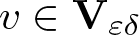 $v\in \textbf{V}_{\varepsilon\delta}$ is arbitrary, we have $v$ satisfy (3.2), which is equivalent to $\nabla v\in \mathrm{SO}(3)$ a.e. in $\Omega^H_{pq}$ for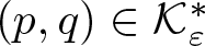 $(p,q)\in{\mathcal{K}}_\varepsilon^*$. So, in summary, every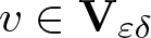 $v\in \textbf{V}_{\varepsilon\delta}$ can be decomposed as (4.35) and we have the estimates as in Lemmas 4.9–4.10, i.e., there exist ${\mathcal{V}}\in H^1({\omega}_\delta)^3$, $\textbf{R}\in H^1({\omega}_\delta)^{3\times 3}$, and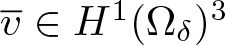 $\overline{v}\in H^1(\Omega_\delta)^3$ such that
 \begin{equation*}v=V_e+\overline{v}={\mathcal{V}}+x_3\textbf{R}\textbf{e}_3+\overline{v},\quad\text{in}\ \Omega_\delta,\end{equation*}
with
 \begin{equation*}\nabla v=\nabla V_e\in \mathrm{SO}(3),\quad \partial_\alpha{\mathcal{V}}-\textbf{R}\textbf{e}_\alpha=0,\quad \overline{v}=0,\quad\text{in}\ \Omega_{\varepsilon\delta}^H.\end{equation*}
Finally, we end this subsection by providing estimates for the corresponding in-plane displacements.
Lemma 4.12. The corresponding displacement  ${\mathcal{U}}={\mathcal{V}}-I_d$ satisfies the following estimates (The constant $C_M$ is introduced such that the assumption (4.61) is satisfied.):
 \begin{equation}
\begin{aligned}
&\|{\mathcal{U}}_3 \|_{H^1({\omega}_\delta)}\leq {C\over \varepsilon^{1/2}\delta}\mathbf{D}(v),\qquad \|\nabla{\mathcal{U}}_\alpha\|_{L^2({\omega}_\delta)}\leq{C\over \delta^{1/2}}\mathbf{D}(v)\Big(1+{\mathbf{D}(v)\over \varepsilon\delta^{3/2}}\Big), \\
& \|{\mathcal{U}}_\alpha\|_{L^2({\omega}_\delta)}\leq{C_M\over \varepsilon^{1/2}}\mathbf{D}(v)\Big(1+{\mathbf{D}(v)\over \varepsilon^{1/2}\delta^2}\Big).
\end{aligned}
\end{equation}
\begin{equation}
\begin{aligned}
&\|{\mathcal{U}}_3 \|_{H^1({\omega}_\delta)}\leq {C\over \varepsilon^{1/2}\delta}\mathbf{D}(v),\qquad \|\nabla{\mathcal{U}}_\alpha\|_{L^2({\omega}_\delta)}\leq{C\over \delta^{1/2}}\mathbf{D}(v)\Big(1+{\mathbf{D}(v)\over \varepsilon\delta^{3/2}}\Big), \\
& \|{\mathcal{U}}_\alpha\|_{L^2({\omega}_\delta)}\leq{C_M\over \varepsilon^{1/2}}\mathbf{D}(v)\Big(1+{\mathbf{D}(v)\over \varepsilon^{1/2}\delta^2}\Big).
\end{aligned}
\end{equation}Moreover, we have
 \begin{equation}
\|{\mathcal{U}}^{\diamond}-{\mathcal{U}}\|_{H^1({\omega}_\delta)}\leq {C\over \delta^{1/2}}\mathbf{D}(v).
\end{equation}
\begin{equation}
\|{\mathcal{U}}^{\diamond}-{\mathcal{U}}\|_{H^1({\omega}_\delta)}\leq {C\over \delta^{1/2}}\mathbf{D}(v).
\end{equation} The constants do not depend on  $\varepsilon$ and $\delta$.
Proof. The estimates (4.37) $_3$ and (4.38) $_{1,2}$ lead to (4.56) $_1$. Observe that due to (4.38) $_1$ and (4.37) $_5$, we have
 \begin{equation}
\|\partial_{\alpha}{\mathcal{V}}-\textbf{R}^\circ\textbf{e}_{\alpha}\|_{L^2({\omega}_\delta)}\leq {C\over \delta^{1/2}}\textbf{D}(v).
\end{equation}
\begin{equation}
\|\partial_{\alpha}{\mathcal{V}}-\textbf{R}^\circ\textbf{e}_{\alpha}\|_{L^2({\omega}_\delta)}\leq {C\over \delta^{1/2}}\textbf{D}(v).
\end{equation}Now, we have
 \begin{equation*}
\big(\partial_\alpha{\mathcal{V}}-\textbf{R}^\circ\textbf{e}_\alpha\big)\cdot\textbf{e}_\beta+\big(\partial_\beta{\mathcal{V}}-\textbf{R}^\circ\textbf{e}_\beta\big)\cdot\textbf{e}_\alpha
=2 e_{\alpha\beta}({\mathcal{U}})-\big((\textbf{R}^\circ)^T+\textbf{R}^\circ-2\textbf{I}_3\big)\textbf{e}_\beta\cdot\textbf{e}_\alpha.
\end{equation*}
\begin{equation*}
\big(\partial_\alpha{\mathcal{V}}-\textbf{R}^\circ\textbf{e}_\alpha\big)\cdot\textbf{e}_\beta+\big(\partial_\beta{\mathcal{V}}-\textbf{R}^\circ\textbf{e}_\beta\big)\cdot\textbf{e}_\alpha
=2 e_{\alpha\beta}({\mathcal{U}})-\big((\textbf{R}^\circ)^T+\textbf{R}^\circ-2\textbf{I}_3\big)\textbf{e}_\beta\cdot\textbf{e}_\alpha.
\end{equation*}Then, the above expression and (4.50), (4.58) imply (similarly, as in Step 3 of Lemma 4.6)
 \begin{equation*}\|e_{\alpha\beta}({\mathcal{U}})\|_{L^2({\omega}_\delta)}\leq {C\over \delta^{1/2}}\textbf{D}(v)\Big(1+{\textbf{D}(v)\over {\varepsilon\delta}^{3/2}}\Big).\end{equation*}
 Since  ${\mathcal{U}}_1$, ${\mathcal{U}}_2$ vanish on $\gamma$, the $2D$ Korn’s inequality gives (4.56) $_2$.
$_2$.
The  ${\cal Q}_1$ character of ${\mathcal{U}}^{\diamond}$ with the estimate (4.19) $_2$ and the estimate (4.26) of $(\textbf{R}^\circ-\textbf{I}_3)\textbf{e}_{\alpha}\cdot\textbf{e}_{\beta}$ gives
 \begin{align}
&\sum_{(p,q)\in{\mathcal{K}}^\ast_\varepsilon}\varepsilon^2|(\textbf{a}_{pq}-p\varepsilon\textbf{e}_1-q\varepsilon\textbf{e}_2)\cdot\textbf{e}_{\alpha}|^2\nonumber\\
&\quad +\sum_{(p,q)\in {\mathcal K}^*_\varepsilon}|(\textbf{R}_{pq}-\textbf{I}_3)\textbf{e}_{\alpha}\cdot\textbf{e}_{\beta}|^2\varepsilon^2\leq {C\over \varepsilon}\Big[\textbf{D}(v)\Big(1+ {\textbf{D}(v)\over \varepsilon^{1/2}\delta^2}\Big)\Big]^2.
\end{align}
\begin{align}
&\sum_{(p,q)\in{\mathcal{K}}^\ast_\varepsilon}\varepsilon^2|(\textbf{a}_{pq}-p\varepsilon\textbf{e}_1-q\varepsilon\textbf{e}_2)\cdot\textbf{e}_{\alpha}|^2\nonumber\\
&\quad +\sum_{(p,q)\in {\mathcal K}^*_\varepsilon}|(\textbf{R}_{pq}-\textbf{I}_3)\textbf{e}_{\alpha}\cdot\textbf{e}_{\beta}|^2\varepsilon^2\leq {C\over \varepsilon}\Big[\textbf{D}(v)\Big(1+ {\textbf{D}(v)\over \varepsilon^{1/2}\delta^2}\Big)\Big]^2.
\end{align} The above estimates and the definition of  ${\cal U}_{\alpha}$ imply
 \begin{equation*}
\|{\cal U}_{\alpha}\|_{L^2({\omega}^H_{{\varepsilon\delta}})}\leq {C\over \varepsilon^{1/2}}\textbf{D}(v)\Big(1+ {\textbf{D}(v)\over \varepsilon^{1/2}\delta^2}\Big).
\end{equation*}
\begin{equation*}
\|{\cal U}_{\alpha}\|_{L^2({\omega}^H_{{\varepsilon\delta}})}\leq {C\over \varepsilon^{1/2}}\textbf{D}(v)\Big(1+ {\textbf{D}(v)\over \varepsilon^{1/2}\delta^2}\Big).
\end{equation*} Then, using (4.9) $_1$ with the above estimate and (4.56) $_2$, we deduce (4.56) $_3$.
$_3$.
We have the following identity
 \begin{equation*}{\partial}_{\alpha}({\cal U}^{\diamond}-{\cal U})=[{\partial}_{\alpha}{\cal U}^{\diamond}-(\textbf{R}^\circ-\textbf{I}_3)\textbf{e}_{\alpha}]-[{\partial}_{\alpha}{\cal U}-(\textbf{R}-\textbf{I}_3)\textbf{e}_{\alpha}]+(\textbf{R}-\textbf{R}^\circ)\textbf{e}_{\alpha}.\end{equation*}
 So, the above identity with the estimates (4.17) $_1$, (4.37) $_5$, and (4.38) $_1$ give
 \begin{equation*}\|{\partial}_{\alpha}({\cal U}^{\diamond}-{\cal U})\|_{L^2({\omega}_\delta)}\leq {C\over \delta^{1/2}}\textbf{D}(v),\end{equation*}
which along with Poincaré inequality gives (4.57). This completes the proof.
Remark 4.13. From the estimates (4.56) $_{1,3}$ satisfied by ${\cal U}_3$ and ${\cal U}_{\alpha}$, we conclude the following: Let us consider any sequence $\{v_{{\varepsilon\delta}}\}_{\varepsilon,\delta}\subset \textbf{V}_{{\varepsilon\delta}}$ of admissible deformations such that
 \begin{equation*}
\textbf{D}(v_{{\varepsilon\delta}}) \le C\,\varepsilon^{1/2}\,\delta^{\kappa}, \qquad \kappa\in\{1,2\}.
\end{equation*}
\begin{equation*}
\textbf{D}(v_{{\varepsilon\delta}}) \le C\,\varepsilon^{1/2}\,\delta^{\kappa}, \qquad \kappa\in\{1,2\}.
\end{equation*} The scaling exponent  $\kappa$ identifies the regime as follows:

Long description
The table presents a classification of deformation regimes associated with two distinct values. The first value is linked to a regime characterized by large deformation, indicating significant changes in shape or structure. The second value corresponds to the von–Kármán critical regime, which is typically associated with specific critical conditions in structural analysis. This categorization helps in understanding the behavior of materials or structures under different conditions. The table does not provide additional context or data points beyond these two classifications, and interpretations should consider the limited scope of the data presented.
In this paper, we analyse an intermediate case (see (4.69) and (6.1)) between large-deformation and von Kármán regime, i.e., lower than large-deformation (bending) regime and higher than von Kármán regime. Keeping estimate (4.56) $_2$ in mind and simplicity of presentation, we choose the order (4.69) and (6.1).
4.3. Estimates for the right-hand side forces
In this subsection, using the estimates derived in previous sections, we derive the upper and lower bounds of the minimization problem using the right-hand side forces. We recall, 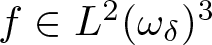 $f\in L^2({\omega}_\delta)^3$, then $f_{\varepsilon\delta}\in L^2(\Omega_\delta)^3$ is given by
 \begin{equation}
f_{\varepsilon\delta}(x)=\sum_{\alpha=1}^2{\varepsilon\delta} f_\alpha(x')\textbf{e}_\alpha+({\varepsilon\delta})^{3/2} f_3(x')\textbf{e}_3,\quad \text{a.e. in}\ \Omega_\delta.
\end{equation}
\begin{equation}
f_{\varepsilon\delta}(x)=\sum_{\alpha=1}^2{\varepsilon\delta} f_\alpha(x')\textbf{e}_\alpha+({\varepsilon\delta})^{3/2} f_3(x')\textbf{e}_3,\quad \text{a.e. in}\ \Omega_\delta.
\end{equation}Then, due to this re-scaling, we have the following lemma.
Lemma 4.14. Assuming
 \begin{equation}
C_M\sum^2_{\beta=1}\|f_\beta\|_{L^2({\omega}_\delta)}\leq{c_0\over 4},
\end{equation}
\begin{equation}
C_M\sum^2_{\beta=1}\|f_\beta\|_{L^2({\omega}_\delta)}\leq{c_0\over 4},
\end{equation}for any 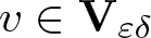 $v\in\textbf{V}_{\varepsilon\delta}$ satisfying $\textbf{J}_{\varepsilon\delta}(v)\leq \textbf{J}_{\varepsilon\delta}(I_d)=0$ we have
 \begin{equation}
\textbf{D}(v)+\|(\nabla v)^T\nabla v-\textbf{I}_3\|_{L^2(\Omega^S_{\varepsilon\delta})}\leq C\varepsilon\delta^{3/2}\|f\|_{L^2({\omega}_\delta)}.
\end{equation}
\begin{equation}
\textbf{D}(v)+\|(\nabla v)^T\nabla v-\textbf{I}_3\|_{L^2(\Omega^S_{\varepsilon\delta})}\leq C\varepsilon\delta^{3/2}\|f\|_{L^2({\omega}_\delta)}.
\end{equation} The constant is independent of  $\varepsilon$ and $\delta$.
Proof. First, using the decomposition (4.35), we have
 \begin{equation}
\begin{aligned}
&\!\!\!\!\int_{\Omega_\delta}f_{\varepsilon\delta}\cdot (v-I_d)\,dx\\
&= \int_{\Omega_\delta}f_{\varepsilon\delta}\cdot\Big(({\mathcal{V}}-I_d)(x')+x_3(\textbf{R}-\textbf{I}_3)(x')\textbf{e}_3\Big)\,dx+\int_{\Omega^S_{\varepsilon\delta}}f_{\varepsilon\delta}\cdot\overline{v}\,dx,\\
&=\delta\int_{{\omega}_\delta}f_{\varepsilon\delta}(x')\cdot({\mathcal{V}}-I_d)(x')\,dx'+\int_{\Omega^S_{\varepsilon\delta}}f_{\varepsilon\delta}\cdot\overline{v}\,dx.
\end{aligned}
\end{equation}
\begin{equation}
\begin{aligned}
&\!\!\!\!\int_{\Omega_\delta}f_{\varepsilon\delta}\cdot (v-I_d)\,dx\\
&= \int_{\Omega_\delta}f_{\varepsilon\delta}\cdot\Big(({\mathcal{V}}-I_d)(x')+x_3(\textbf{R}-\textbf{I}_3)(x')\textbf{e}_3\Big)\,dx+\int_{\Omega^S_{\varepsilon\delta}}f_{\varepsilon\delta}\cdot\overline{v}\,dx,\\
&=\delta\int_{{\omega}_\delta}f_{\varepsilon\delta}(x')\cdot({\mathcal{V}}-I_d)(x')\,dx'+\int_{\Omega^S_{\varepsilon\delta}}f_{\varepsilon\delta}\cdot\overline{v}\,dx.
\end{aligned}
\end{equation} First observe that the expression (4.60) and the estimate (4.38) $_3$ give
 \begin{equation}
\left|\int_{\Omega^S_{\varepsilon\delta}}f_{\varepsilon\delta}\cdot \overline{v}\,dx\right|\leq \delta^{1/2}\|f_{\varepsilon\delta}\|_{L^2({\omega}_\delta)}\|\overline{v}\|_{L^2(\Omega_\delta)}\leq C\varepsilon\delta^{3/2}\|f\|_{L^2({\omega}_\delta)}\textbf{D}(v).
\end{equation}
\begin{equation}
\left|\int_{\Omega^S_{\varepsilon\delta}}f_{\varepsilon\delta}\cdot \overline{v}\,dx\right|\leq \delta^{1/2}\|f_{\varepsilon\delta}\|_{L^2({\omega}_\delta)}\|\overline{v}\|_{L^2(\Omega_\delta)}\leq C\varepsilon\delta^{3/2}\|f\|_{L^2({\omega}_\delta)}\textbf{D}(v).
\end{equation} Again the estimates (4.56) $_{1,3}$ give
 \begin{equation}
{\begin{aligned}
\delta\left|\int_{{\omega}_{\delta}}f_{\varepsilon\delta}\cdot ({\mathcal{V}}-I_d)\,dx'\right|
&\leq \delta\|f_{\varepsilon\delta,3}\|_{L^2({\omega}_\delta)}\|{\mathcal{U}}_3\|_{L^2({\omega}_\delta)}+\delta\sum_{\alpha=1}^2\|f_{\varepsilon\delta,\alpha}\|_{L^2({\omega}_\delta)}\|{\mathcal{U}}_\alpha\|_{L^2({\omega}_\delta)}\\
&\leq C\varepsilon^{1/2}\delta^{3/2}(\varepsilon^{1/2}+\delta^{1/2})\textbf{D}(v)\|f\|_{L^2({\omega}_\delta)}\\
&\quad +C_M\Big(\sum_{\alpha=1}^2\|f_\alpha\|_{L^2({\omega}_\delta)}\Big)\textbf{D}(v)^2.
\end{aligned}
}
\end{equation}
\begin{equation}
{\begin{aligned}
\delta\left|\int_{{\omega}_{\delta}}f_{\varepsilon\delta}\cdot ({\mathcal{V}}-I_d)\,dx'\right|
&\leq \delta\|f_{\varepsilon\delta,3}\|_{L^2({\omega}_\delta)}\|{\mathcal{U}}_3\|_{L^2({\omega}_\delta)}+\delta\sum_{\alpha=1}^2\|f_{\varepsilon\delta,\alpha}\|_{L^2({\omega}_\delta)}\|{\mathcal{U}}_\alpha\|_{L^2({\omega}_\delta)}\\
&\leq C\varepsilon^{1/2}\delta^{3/2}(\varepsilon^{1/2}+\delta^{1/2})\textbf{D}(v)\|f\|_{L^2({\omega}_\delta)}\\
&\quad +C_M\Big(\sum_{\alpha=1}^2\|f_\alpha\|_{L^2({\omega}_\delta)}\Big)\textbf{D}(v)^2.
\end{aligned}
}
\end{equation}We recall that
 \begin{equation}
\mathrm{dist}(F, \mathrm{SO}(3))\leq |F^TF-\textbf{I}_3| \quad \text{for all}\;\;F \in \textbf{M}_3\quad\hbox{such that}\;\; \mathrm{det}(F) \gt 0,
\end{equation}
\begin{equation}
\mathrm{dist}(F, \mathrm{SO}(3))\leq |F^TF-\textbf{I}_3| \quad \text{for all}\;\;F \in \textbf{M}_3\quad\hbox{such that}\;\; \mathrm{det}(F) \gt 0,
\end{equation}and due to the assumption (3.6), we have
 \begin{equation}
c_0|F^{T}F-\textbf{I}_3|^2\leq \textbf{Q}_{\varepsilon\delta}\big(x , \textbf{E}(F)\big)\qquad \hbox{for a.e. } x\in \Omega^S_{\varepsilon\delta},\quad \forall\,F\in\textbf{M}_3.
\end{equation}
\begin{equation}
c_0|F^{T}F-\textbf{I}_3|^2\leq \textbf{Q}_{\varepsilon\delta}\big(x , \textbf{E}(F)\big)\qquad \hbox{for a.e. } x\in \Omega^S_{\varepsilon\delta},\quad \forall\,F\in\textbf{M}_3.
\end{equation} Since we have  $\textbf{J}_{\varepsilon\delta}(v)\leq \textbf{J}_{\varepsilon\delta}(I_d)=0$, then using the two inequalities (4.66)–(4.67), we obtain
 \begin{align*}&c_0\textbf{D}(v)^2-\int_{\Omega_{\delta}}f_{\varepsilon\delta}\cdot(v-I_d)\,dx\leq c_0\|(\nabla v)^T(\nabla v)-\textbf{I}_3\|^2_{L^2(\Omega^S_{\varepsilon\delta})}\\
&\quad -\int_{\Omega_{\delta}}f_{\varepsilon\delta}\cdot(v-I_d)\,dx\leq \textbf{J}_{\varepsilon\delta}(v)\leq 0\end{align*}
\begin{align*}&c_0\textbf{D}(v)^2-\int_{\Omega_{\delta}}f_{\varepsilon\delta}\cdot(v-I_d)\,dx\leq c_0\|(\nabla v)^T(\nabla v)-\textbf{I}_3\|^2_{L^2(\Omega^S_{\varepsilon\delta})}\\
&\quad -\int_{\Omega_{\delta}}f_{\varepsilon\delta}\cdot(v-I_d)\,dx\leq \textbf{J}_{\varepsilon\delta}(v)\leq 0\end{align*}which imply
 \begin{align}
&c_0\|(\nabla v)^T(\nabla v)-\textbf{I}_3\|^2_{L^2(\Omega^S_{\varepsilon\delta})}\leq \left|\int_{\Omega_{\delta}}f_{\varepsilon\delta}\cdot (v-I_d)\,dx\right|, \nonumber\\
&c_0\textbf{D}(v)^2\leq 2 \left|\int_{\Omega_{\delta}}f_{\varepsilon\delta}\cdot (v-I_d)\,dx\right|.
\end{align}
\begin{align}
&c_0\|(\nabla v)^T(\nabla v)-\textbf{I}_3\|^2_{L^2(\Omega^S_{\varepsilon\delta})}\leq \left|\int_{\Omega_{\delta}}f_{\varepsilon\delta}\cdot (v-I_d)\,dx\right|, \nonumber\\
&c_0\textbf{D}(v)^2\leq 2 \left|\int_{\Omega_{\delta}}f_{\varepsilon\delta}\cdot (v-I_d)\,dx\right|.
\end{align}Therefore, the above inequalities with (4.64)–(4.65) give
 \begin{equation*}
c_0\textbf{D}(v)^2 \leq C\varepsilon\delta^{3/2}\textbf{D}(v)\|f\|_{L^2({\omega}_\delta)}+ 2C_M\Big(\sum_{\alpha=1}^2\|f_\alpha\|_{L^2({\omega}_\delta)}\Big)\textbf{D}(v)^2.
\end{equation*}
\begin{equation*}
c_0\textbf{D}(v)^2 \leq C\varepsilon\delta^{3/2}\textbf{D}(v)\|f\|_{L^2({\omega}_\delta)}+ 2C_M\Big(\sum_{\alpha=1}^2\|f_\alpha\|_{L^2({\omega}_\delta)}\Big)\textbf{D}(v)^2.
\end{equation*}So, with the assumption (4.61) and the inequalities (4.68), we obtain the estimates (4.62).
Remark 4.15. As a consequence of the above lemma, we have that there exist constants 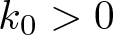 $k_0 \gt 0$ independent of $\varepsilon$ and $\delta$ such that
 \begin{equation*}-k_0\varepsilon^2\delta^3\leq \textbf{J}_{\varepsilon\delta}(v)\leq \textbf{J}_{\varepsilon\delta}(I_d)=0,\end{equation*}
which in turn give
 \begin{equation}
-k_0\leq {\textbf{m}_{\varepsilon\delta}\over \varepsilon^2\delta^3}\leq 0.
\end{equation}
\begin{equation}
-k_0\leq {\textbf{m}_{\varepsilon\delta}\over \varepsilon^2\delta^3}\leq 0.
\end{equation} In the subsequent subsections, we characterize the limit of the sequence 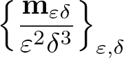 $\displaystyle\left\{{\textbf{m}_{\varepsilon\delta}\over \varepsilon^2\delta^3}\right\}_{\varepsilon,\delta}$ as $\varepsilon$ and $\delta$ tend to zero, as the minimum of a functional. Observe that from (4.69), we have that there exists a sequence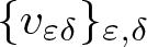 $\{v_{{\varepsilon\delta}}\}_{\varepsilon,\delta}$ in $\textbf{V}_{\varepsilon\delta}$ such that
 \begin{equation*}
\liminf_{(\varepsilon,\delta)\to(0,0)}{\textbf{m}_{\varepsilon\delta}\over \varepsilon^2\delta^3}=\lim_{(\varepsilon,\delta)\to(0,0)}{\textbf{J}_{\varepsilon\delta}(v_{\varepsilon\delta})\over \varepsilon^2\delta^3}.
\end{equation*}
\begin{equation*}
\liminf_{(\varepsilon,\delta)\to(0,0)}{\textbf{m}_{\varepsilon\delta}\over \varepsilon^2\delta^3}=\lim_{(\varepsilon,\delta)\to(0,0)}{\textbf{J}_{\varepsilon\delta}(v_{\varepsilon\delta})\over \varepsilon^2\delta^3}.
\end{equation*} Without loss of generality, we can assume that  $\textbf{J}_{\varepsilon\delta}(v_{\varepsilon\delta})\leq \textbf{J}_{\varepsilon\delta}(I_d)=0$.
So, the rescaling of forces (4.60) is chosen in such a way that the total energy remains in the intermediate regime (4.69). Hence, the order of the total energy depends directly on the scaling of forces. Similar type of scaling of forces is present in [Reference Blanchard and Griso1, Reference Chakrabortty, Griso and Orlik4, Reference Falconi, Griso and Orlik17, Reference Griso, Orlik and Wackerle22] to get the order of the microscopic total energy.
5. Unfolding operators and their properties
In this section, we introduce two rescaled unfolding operators, which play a central role in deriving the asymptotic limits.
Definition 5.1. (
$3$D rescaled unfolding operators)

For every measurable function  $\psi$ on $\Omega_{\varepsilon\delta}^{(1)}$ (resp. $\Omega_{\varepsilon\delta}^{(2)}$), we define the measurable functions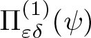 $\Pi^{(1)}_{\varepsilon\delta}(\psi)$ (resp.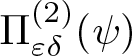 $\Pi^{(2)}_{\varepsilon\delta}(\psi)$) by
 \begin{equation}
\begin{aligned}
\Pi^{(1)}_{\varepsilon\delta}(\psi) (x',y) & \doteq \psi \Big(\varepsilon\Big[{x'\over \varepsilon}\Big]+ \varepsilon y_1\textbf{e}_1+\delta y_2\textbf{e}_2,\delta y_3\Big) \\
&\quad \text{for a.e.}\;(x',y)\in{\omega}\times {\mathcal{Y}}_1,\\
\hbox{(resp. }\; \Pi^{(2)}_{\varepsilon\delta}(\psi) (x',y) & \doteq \psi \Big(\varepsilon\Big[{x'\over \varepsilon}\Big]+ \delta y_1\textbf{e}_1+\varepsilon y_2\textbf{e}_2,\delta y_3\Big)\\
&\quad \text{for a.e.}\;(x',y)\in{\omega}\times {\mathcal{Y}}_2\hbox{)}.
\end{aligned}
\end{equation}
\begin{equation}
\begin{aligned}
\Pi^{(1)}_{\varepsilon\delta}(\psi) (x',y) & \doteq \psi \Big(\varepsilon\Big[{x'\over \varepsilon}\Big]+ \varepsilon y_1\textbf{e}_1+\delta y_2\textbf{e}_2,\delta y_3\Big) \\
&\quad \text{for a.e.}\;(x',y)\in{\omega}\times {\mathcal{Y}}_1,\\
\hbox{(resp. }\; \Pi^{(2)}_{\varepsilon\delta}(\psi) (x',y) & \doteq \psi \Big(\varepsilon\Big[{x'\over \varepsilon}\Big]+ \delta y_1\textbf{e}_1+\varepsilon y_2\textbf{e}_2,\delta y_3\Big)\\
&\quad \text{for a.e.}\;(x',y)\in{\omega}\times {\mathcal{Y}}_2\hbox{)}.
\end{aligned}
\end{equation} Below, we recall some of the properties and inequalities related to the  $3$D rescaled unfolding operator. For more details, see [Reference Griso, Orlik and Wackerle21] and [Reference Orlik, Falconi, Griso and Wackerle27]. $\bullet$ For every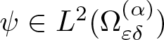 $\psi\in L^2(\Omega_{\varepsilon\delta}^{(\alpha)})$, we have
 \begin{equation}
\|\Pi^{(\alpha)}_{\varepsilon\delta}(\psi)\|_{L^2({\omega}\times {\mathcal{Y}}_\alpha)}\leq {\sqrt\varepsilon\over \delta}\|\psi\|_{L^2(\Omega_{\varepsilon\delta}^{(\alpha)})}.
\end{equation}
\begin{equation}
\|\Pi^{(\alpha)}_{\varepsilon\delta}(\psi)\|_{L^2({\omega}\times {\mathcal{Y}}_\alpha)}\leq {\sqrt\varepsilon\over \delta}\|\psi\|_{L^2(\Omega_{\varepsilon\delta}^{(\alpha)})}.
\end{equation}  $\bullet$ For any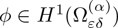 $\phi\in H^1(\Omega_{\varepsilon\delta}^{(\alpha)})$, one has
 \begin{align}
&{\partial\Pi^{(\alpha)}_{\varepsilon\delta}(\phi)\over \partial y_\alpha}=\varepsilon\Pi^{(\alpha)}_{\varepsilon\delta}\big({\partial \phi\over \partial x_\alpha}\big),\quad {\partial\Pi^{(\alpha)}_{\varepsilon\delta}(\phi)\over \partial y_{3-\alpha}}=\delta\Pi^{(\alpha)}_{\varepsilon\delta}\big({\partial \phi\over \partial x_{3-\alpha}}\big),\nonumber\\ &{\partial\Pi^{(\alpha)}_{\varepsilon\delta}(\phi)\over \partial y_3}=\delta\Pi^{(\alpha)}_{\varepsilon\delta}\big({\partial \phi\over \partial x_3}\big).
\end{align}
\begin{align}
&{\partial\Pi^{(\alpha)}_{\varepsilon\delta}(\phi)\over \partial y_\alpha}=\varepsilon\Pi^{(\alpha)}_{\varepsilon\delta}\big({\partial \phi\over \partial x_\alpha}\big),\quad {\partial\Pi^{(\alpha)}_{\varepsilon\delta}(\phi)\over \partial y_{3-\alpha}}=\delta\Pi^{(\alpha)}_{\varepsilon\delta}\big({\partial \phi\over \partial x_{3-\alpha}}\big),\nonumber\\ &{\partial\Pi^{(\alpha)}_{\varepsilon\delta}(\phi)\over \partial y_3}=\delta\Pi^{(\alpha)}_{\varepsilon\delta}\big({\partial \phi\over \partial x_3}\big).
\end{align}Definition 5.2. (
$2$D rescaled unfolding operators)

For every measurable function  $\psi$ on ${\omega}^{(1)}_{\varepsilon\delta}$ (resp. ${\omega}^{(2)}_{\varepsilon\delta}$), we define the measurable functions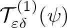 $\mathcal{T}_{\varepsilon\delta}^{(1)}(\psi)$ (resp.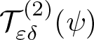 $\mathcal{T}_{\varepsilon\delta}^{(2)}(\psi)$) by
 \begin{equation}
\begin{aligned}
\mathcal{T}_{\varepsilon\delta}^{(1)}(\psi) (x',y') & \doteq \psi \Big(\varepsilon\Big[{x'\over \varepsilon}\Big]+ \varepsilon y_1\mathbf{e}_1+\delta y_2\mathbf{e}_2\Big)\qquad\mathbf{for\ a.e.}\;(x',y')\in{\omega}\times Y_1,\\
\hbox{(resp. }\; \mathcal{T}_{\varepsilon\delta}^{(2)}(\psi) (x',y') & \doteq \psi \Big(\varepsilon\Big[{x'\over \varepsilon}\Big]+ \delta y_1\mathbf{e}_1+\varepsilon y_2\mathbf{e}_2\Big)\qquad\mathbf{for\ a.e.}\;(x',y')\in{\omega}\times Y_2\hbox{)}.
\end{aligned}
\end{equation}
\begin{equation}
\begin{aligned}
\mathcal{T}_{\varepsilon\delta}^{(1)}(\psi) (x',y') & \doteq \psi \Big(\varepsilon\Big[{x'\over \varepsilon}\Big]+ \varepsilon y_1\mathbf{e}_1+\delta y_2\mathbf{e}_2\Big)\qquad\mathbf{for\ a.e.}\;(x',y')\in{\omega}\times Y_1,\\
\hbox{(resp. }\; \mathcal{T}_{\varepsilon\delta}^{(2)}(\psi) (x',y') & \doteq \psi \Big(\varepsilon\Big[{x'\over \varepsilon}\Big]+ \delta y_1\mathbf{e}_1+\varepsilon y_2\mathbf{e}_2\Big)\qquad\mathbf{for\ a.e.}\;(x',y')\in{\omega}\times Y_2\hbox{)}.
\end{aligned}
\end{equation} Below, we briefly give the properties of the  $2$D re-scaling unfolding operator. $\bullet$ For every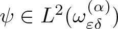 $\psi\in L^2({\omega}_{\varepsilon\delta}^{(\alpha)})$, we have
 \begin{equation}
\|\mathcal{T}_{\varepsilon\delta}^{(\alpha)}(\psi)\|_{L^2({\omega}\times Y_\alpha)}\leq \sqrt{\varepsilon\over \delta}\|\psi\|_{L^2({\omega}_{\varepsilon\delta}^{(\alpha)})}.
\end{equation}
\begin{equation}
\|\mathcal{T}_{\varepsilon\delta}^{(\alpha)}(\psi)\|_{L^2({\omega}\times Y_\alpha)}\leq \sqrt{\varepsilon\over \delta}\|\psi\|_{L^2({\omega}_{\varepsilon\delta}^{(\alpha)})}.
\end{equation}  $\bullet$ For any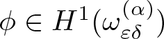 $\phi\in H^1({\omega}_{\varepsilon\delta}^{(\alpha)})$, one has
 \begin{equation*}
{\partial\mathcal{T}_{\varepsilon\delta}^{(\alpha)}(\phi)\over \partial y_\alpha}=\varepsilon\mathcal{T}_{\varepsilon\delta}^{(\alpha)}\Big({\partial \phi\over \partial x_\alpha}\Big),\quad {\partial\mathcal{T}_{\varepsilon\delta}^{(\alpha)}(\phi)\over \partial y_{3-\alpha}}=\delta\mathcal{T}_{\varepsilon\delta}^{(\alpha)}\Big({\partial \phi\over \partial x_{3-\alpha}}\Big).
\end{equation*}
\begin{equation*}
{\partial\mathcal{T}_{\varepsilon\delta}^{(\alpha)}(\phi)\over \partial y_\alpha}=\varepsilon\mathcal{T}_{\varepsilon\delta}^{(\alpha)}\Big({\partial \phi\over \partial x_\alpha}\Big),\quad {\partial\mathcal{T}_{\varepsilon\delta}^{(\alpha)}(\phi)\over \partial y_{3-\alpha}}=\delta\mathcal{T}_{\varepsilon\delta}^{(\alpha)}\Big({\partial \phi\over \partial x_{3-\alpha}}\Big).
\end{equation*}  $\bullet$ For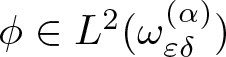 $\phi\in L^2({\omega}^{(\alpha)}_{\varepsilon\delta})$, we have
 \begin{equation*}\begin{aligned}
\Pi_{\varepsilon\delta}^{(\alpha)}(\phi)(x',y',0)=\mathcal{T}_{\varepsilon\delta}^{(\alpha)}(x',y').
\end{aligned}
\end{equation*}
\begin{equation*}\begin{aligned}
\Pi_{\varepsilon\delta}^{(\alpha)}(\phi)(x',y',0)=\mathcal{T}_{\varepsilon\delta}^{(\alpha)}(x',y').
\end{aligned}
\end{equation*}6. Asymptotic limit of the Green–St. Venant’s strain tensor
In this section, we present the limit of the Green–St. Venant strain tensor when both  $\varepsilon$ and $\delta$ tend to zero simultaneously, satisfying (2.2). To this end, we consider a sequence of admissible deformations $\{v_{\varepsilon\delta}\}_{\varepsilon,\delta}\subset \textbf{V}_{\varepsilon\delta}$ such that
 \begin{equation}
\textbf{D}(v_{\varepsilon\delta})\leq C \varepsilon\delta^{3/2}.
\end{equation}
\begin{equation}
\textbf{D}(v_{\varepsilon\delta})\leq C \varepsilon\delta^{3/2}.
\end{equation} The constant is independent of  $\varepsilon$ and $\delta$.
Then, we decompose each  $v_{\varepsilon\delta}$ using (4.35). Using Remark 4.11 and the estimates in Lemmas 4.9–4.12, we obtain (with ${\mathcal{U}}_{\varepsilon\delta}={\mathcal{V}}_{\varepsilon\delta}-I_d$)
 \begin{align}
\begin{aligned}
&\|\textbf{R}_{\varepsilon\delta}-\textbf{I}_3\|_{L^2({\omega}_\delta)} +\|{\mathcal{U}}_{{\varepsilon\delta},3}\|_{H^1({\omega}_\delta)}\leq C\sqrt{\varepsilon\delta},\\
&\|\partial_\alpha{\mathcal{U}}_{\varepsilon\delta}-(\textbf{R}_{\varepsilon\delta}-\textbf{I}_3)\textbf{e}_\alpha\|_{L^2({\omega}_\delta)}\leq C\varepsilon\delta,\quad \|{\mathcal{U}}_{{\varepsilon\delta},\alpha}\|_{H^1({\omega}_\delta)}\leq C{\varepsilon\delta}, \\
&\|(\textbf{R}_{\varepsilon\delta})^T+\textbf{R}_{\varepsilon\delta}-2\textbf{I}_3\|_{L^2({\omega}_\delta)}+\|\textbf{R}_{\varepsilon\delta}(\textbf{R}_{\varepsilon\delta})^T-\textbf{I}_3\|_{L^2({\omega}_\delta)}\leq C{\varepsilon\delta},\\
&\quad \|\nabla \textbf{R}\|_{L^2({\omega}_\delta)}\leq C\varepsilon.
\end{aligned}
\end{align}
\begin{align}
\begin{aligned}
&\|\textbf{R}_{\varepsilon\delta}-\textbf{I}_3\|_{L^2({\omega}_\delta)} +\|{\mathcal{U}}_{{\varepsilon\delta},3}\|_{H^1({\omega}_\delta)}\leq C\sqrt{\varepsilon\delta},\\
&\|\partial_\alpha{\mathcal{U}}_{\varepsilon\delta}-(\textbf{R}_{\varepsilon\delta}-\textbf{I}_3)\textbf{e}_\alpha\|_{L^2({\omega}_\delta)}\leq C\varepsilon\delta,\quad \|{\mathcal{U}}_{{\varepsilon\delta},\alpha}\|_{H^1({\omega}_\delta)}\leq C{\varepsilon\delta}, \\
&\|(\textbf{R}_{\varepsilon\delta})^T+\textbf{R}_{\varepsilon\delta}-2\textbf{I}_3\|_{L^2({\omega}_\delta)}+\|\textbf{R}_{\varepsilon\delta}(\textbf{R}_{\varepsilon\delta})^T-\textbf{I}_3\|_{L^2({\omega}_\delta)}\leq C{\varepsilon\delta},\\
&\quad \|\nabla \textbf{R}\|_{L^2({\omega}_\delta)}\leq C\varepsilon.
\end{aligned}
\end{align} Furthermore, from (4.5) and (4.38) $_{6,7}$, we also have
 \begin{equation}
\|\overline{v}_{\varepsilon\delta}\|_{L^2(\Omega_{\delta})}+\delta\|\nabla \overline{v}_{\varepsilon\delta}\|_{L^2(\Omega_{\delta})} \leq C\varepsilon\delta^{5/2}.
\end{equation}
\begin{equation}
\|\overline{v}_{\varepsilon\delta}\|_{L^2(\Omega_{\delta})}+\delta\|\nabla \overline{v}_{\varepsilon\delta}\|_{L^2(\Omega_{\delta})} \leq C\varepsilon\delta^{5/2}.
\end{equation}Using the properties of the rescaled unfolding operators (5.2)–(5.3), we obtain
 \begin{equation}
\begin{aligned}
\|\Pi^{(\alpha)}_{\varepsilon\delta}(\overline{v}_{\varepsilon\delta})\|_{L^2({\omega}\times {\mathcal{Y}}_\alpha)}+\|\partial_{y_3}(\Pi^{(\alpha)}_{\varepsilon\delta}( \overline{v}_{\varepsilon\delta}))\|_{L^2({\omega}\times {\mathcal{Y}}_\alpha)}\\
+\|\partial_{y_{3-\alpha}}\big(\Pi_{\varepsilon\delta}^{(\alpha)}(\overline{v}_{\varepsilon\delta})\big)\|_{L^2({\omega}\times {\mathcal{Y}}_\alpha)}\leq C{\varepsilon\delta}\sqrt{\varepsilon\delta},\\
\|\partial_{y_\alpha}(\Pi^{(\alpha)}_{\varepsilon\delta}( \overline{v}_{\varepsilon\delta}))\|_{L^2({\omega}\times {\mathcal{Y}}_\alpha)}\leq C\varepsilon^2\sqrt{\varepsilon\delta}.
\end{aligned}
\end{equation}
\begin{equation}
\begin{aligned}
\|\Pi^{(\alpha)}_{\varepsilon\delta}(\overline{v}_{\varepsilon\delta})\|_{L^2({\omega}\times {\mathcal{Y}}_\alpha)}+\|\partial_{y_3}(\Pi^{(\alpha)}_{\varepsilon\delta}( \overline{v}_{\varepsilon\delta}))\|_{L^2({\omega}\times {\mathcal{Y}}_\alpha)}\\
+\|\partial_{y_{3-\alpha}}\big(\Pi_{\varepsilon\delta}^{(\alpha)}(\overline{v}_{\varepsilon\delta})\big)\|_{L^2({\omega}\times {\mathcal{Y}}_\alpha)}\leq C{\varepsilon\delta}\sqrt{\varepsilon\delta},\\
\|\partial_{y_\alpha}(\Pi^{(\alpha)}_{\varepsilon\delta}( \overline{v}_{\varepsilon\delta}))\|_{L^2({\omega}\times {\mathcal{Y}}_\alpha)}\leq C\varepsilon^2\sqrt{\varepsilon\delta}.
\end{aligned}
\end{equation} The constant(s) above are independent of  $\varepsilon$ and $\delta$.
First, in Subsection 6.1, we derive the limit (In all the lemmas below, we extract a subsequence of 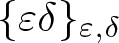 $\{{\varepsilon\delta}\}_{\varepsilon,\delta}$ [still denoted by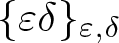 $\{{\varepsilon\delta}\}_{\varepsilon,\delta}$] to get the desired convergences.) macroscopic fields using (6.2). Then, in Subsection 6.2, by applying the unfolding operators and the estimates (6.2)–(6.4), we characterize the limits of both macroscopic and microscopic fields. Finally, in Theorem 6.4, we establish the limit of the Green–St. Venant strain tensor.
6.1. Limit behaviour of the macroscopic fields
The limit spaces for macroscopic fields are given by
 \begin{equation*}\begin{aligned}
&H^1_\gamma({\omega}) \doteq \left\{\phi\in H^1({\omega})\;\;|\;\;\phi=0\quad\text{a.e. on}\ \gamma\right\},\\
& H^2_\gamma({\omega}) \doteq \left\{\phi\in H^2({\omega})\;\;|\;\;\phi=\partial_\alpha\phi=0\quad\text{a.e. on}\ \gamma\right\},\\
&L^2({\omega},\partial_\alpha)\doteq \big\{\psi\in L^2({\omega})\;|\; \partial_\alpha\psi\in L^2({\omega})\big\},\\
& H^1({\omega};\partial_{12})\doteq \big\{\psi\in H^1({\omega})\,|\,\partial_{12}\psi\in L^2({\omega})\},\\
&H_{(0,l)}^{1}\big((0,L)_{x_\alpha}\big)\doteq \big\{\psi(x_\alpha)\in H^1(0,L)\;|\; \psi=0\quad \hbox{a.e. in } (0,l)\,\big\},\\
&H_{(0,l)}^{2}\big((0,L)_{x_\alpha}\big)\doteq \big\{\psi(x_\alpha)\in H^2(0,L)\;|\; \psi=0\quad \hbox{a.e. in } (0,l)\,\big\}.
\end{aligned}
\end{equation*}
\begin{equation*}\begin{aligned}
&H^1_\gamma({\omega}) \doteq \left\{\phi\in H^1({\omega})\;\;|\;\;\phi=0\quad\text{a.e. on}\ \gamma\right\},\\
& H^2_\gamma({\omega}) \doteq \left\{\phi\in H^2({\omega})\;\;|\;\;\phi=\partial_\alpha\phi=0\quad\text{a.e. on}\ \gamma\right\},\\
&L^2({\omega},\partial_\alpha)\doteq \big\{\psi\in L^2({\omega})\;|\; \partial_\alpha\psi\in L^2({\omega})\big\},\\
& H^1({\omega};\partial_{12})\doteq \big\{\psi\in H^1({\omega})\,|\,\partial_{12}\psi\in L^2({\omega})\},\\
&H_{(0,l)}^{1}\big((0,L)_{x_\alpha}\big)\doteq \big\{\psi(x_\alpha)\in H^1(0,L)\;|\; \psi=0\quad \hbox{a.e. in } (0,l)\,\big\},\\
&H_{(0,l)}^{2}\big((0,L)_{x_\alpha}\big)\doteq \big\{\psi(x_\alpha)\in H^2(0,L)\;|\; \psi=0\quad \hbox{a.e. in } (0,l)\,\big\}.
\end{aligned}
\end{equation*}The following convergences hold for the macroscopic fields:
Lemma 6.1. There exist  ${\mathcal{U}}=({\mathcal{U}}_1,\,{\mathcal{U}}_2,{\mathcal{U}}_3)\in H^1_\gamma({\omega})^3$, $\mathbf{A}\in L^2({\omega})^{3\times 3}$ such that
 \begin{equation}
\begin{aligned}
{1\over \varepsilon\delta}{\mathcal{U}}_{{\varepsilon\delta},\alpha}&\rightharpoonup {\mathcal{U}}_\alpha\quad &&\text{weakly in}\ H^1({\omega}),\\
{1\over ({\varepsilon\delta})^{1/2}}{\mathcal{U}}_{{\varepsilon\delta},3}&\to {\mathcal{U}}_3\quad&&\text{strongly in}\ H^1({\omega}),\\
{1\over ({\varepsilon\delta})^{1/2}}(\mathbf{R}_{\varepsilon\delta}-\mathbf{I}_3)&\rightharpoonup \mathbf{A}\quad &&\text{weakly in}\ L^2({\omega})^{3\times 3},
\end{aligned}
\end{equation}
\begin{equation}
\begin{aligned}
{1\over \varepsilon\delta}{\mathcal{U}}_{{\varepsilon\delta},\alpha}&\rightharpoonup {\mathcal{U}}_\alpha\quad &&\text{weakly in}\ H^1({\omega}),\\
{1\over ({\varepsilon\delta})^{1/2}}{\mathcal{U}}_{{\varepsilon\delta},3}&\to {\mathcal{U}}_3\quad&&\text{strongly in}\ H^1({\omega}),\\
{1\over ({\varepsilon\delta})^{1/2}}(\mathbf{R}_{\varepsilon\delta}-\mathbf{I}_3)&\rightharpoonup \mathbf{A}\quad &&\text{weakly in}\ L^2({\omega})^{3\times 3},
\end{aligned}
\end{equation}with
 \begin{equation}
\begin{aligned}
\mathbf{A}=-\mathbf{A}^T,\quad \partial_\alpha{\mathcal{U}}_3=\mathbf{A}\mathbf{e}_\alpha\cdot\mathbf{e}_3,\quad {\mathcal{U}}_3\in H^2_\gamma({\omega}),\quad\text{with}\quad\partial_{12}{\mathcal{U}}_3=0.
\end{aligned}
\end{equation}
\begin{equation}
\begin{aligned}
\mathbf{A}=-\mathbf{A}^T,\quad \partial_\alpha{\mathcal{U}}_3=\mathbf{A}\mathbf{e}_\alpha\cdot\mathbf{e}_3,\quad {\mathcal{U}}_3\in H^2_\gamma({\omega}),\quad\text{with}\quad\partial_{12}{\mathcal{U}}_3=0.
\end{aligned}
\end{equation} Moreover, there exist  ${\mathcal{R}}^{(1)}\in L^2({\omega};\partial_2)^3$, ${\mathcal{R}}^{(2)}\in L^2({\omega};\partial_1)^3$, and $U\in H^1({\omega};\partial_{12})^3$ such that
 \begin{equation}
\begin{aligned}
{\varepsilon\over\delta}{1\over \sqrt{{\varepsilon\delta}}}\big((\mathbf{R}^{\diamond}_{\varepsilon\delta}-\mathbf{I}_3)\mathbf{e}_1-d_1F^{\diamond}\big)&\rightharpoonup {\mathcal{R}}^{(1)},\quad &&\text{weakly in}\ L^2({\omega})^3,\\
{\varepsilon\over\delta}{1\over \sqrt{{\varepsilon\delta}}}\big((\mathbf{R}^{\diamond}_{\varepsilon\delta}-\mathbf{I}_3)\mathbf{e}_2-d_2G^{\diamond}_{\varepsilon\delta}\big)&\rightharpoonup {\mathcal{R}}^{(2)},\quad &&\text{weakly in}\ L^2({\omega})^3,\\
{\varepsilon\over\delta}{1\over\sqrt{{\varepsilon\delta}}}\,\big({\mathcal{U}}^{\diamond}_{\varepsilon\delta}-F^{\diamond}_{\varepsilon\delta}-G^{\diamond}_{\varepsilon\delta}\big)&\rightharpoonup U,\quad &&\text{weakly in}\ H^1({\omega})^3,
\end{aligned}
\end{equation}
\begin{equation}
\begin{aligned}
{\varepsilon\over\delta}{1\over \sqrt{{\varepsilon\delta}}}\big((\mathbf{R}^{\diamond}_{\varepsilon\delta}-\mathbf{I}_3)\mathbf{e}_1-d_1F^{\diamond}\big)&\rightharpoonup {\mathcal{R}}^{(1)},\quad &&\text{weakly in}\ L^2({\omega})^3,\\
{\varepsilon\over\delta}{1\over \sqrt{{\varepsilon\delta}}}\big((\mathbf{R}^{\diamond}_{\varepsilon\delta}-\mathbf{I}_3)\mathbf{e}_2-d_2G^{\diamond}_{\varepsilon\delta}\big)&\rightharpoonup {\mathcal{R}}^{(2)},\quad &&\text{weakly in}\ L^2({\omega})^3,\\
{\varepsilon\over\delta}{1\over\sqrt{{\varepsilon\delta}}}\,\big({\mathcal{U}}^{\diamond}_{\varepsilon\delta}-F^{\diamond}_{\varepsilon\delta}-G^{\diamond}_{\varepsilon\delta}\big)&\rightharpoonup U,\quad &&\text{weakly in}\ H^1({\omega})^3,
\end{aligned}
\end{equation}with
 \begin{equation}
\begin{aligned}
&\partial_\alpha U = {\mathcal{R}}^{(\alpha)},\quad \partial_{12}U=\partial_1{\mathcal{R}}^{(2)}=\partial_2{\mathcal{R}}^{(1)},\quad\text{a.e. in}\ {\omega},\quad U=0,\quad\text{on}\ \gamma.
\end{aligned}
\end{equation}
\begin{equation}
\begin{aligned}
&\partial_\alpha U = {\mathcal{R}}^{(\alpha)},\quad \partial_{12}U=\partial_1{\mathcal{R}}^{(2)}=\partial_2{\mathcal{R}}^{(1)},\quad\text{a.e. in}\ {\omega},\quad U=0,\quad\text{on}\ \gamma.
\end{aligned}
\end{equation}Proof. All the convergences (6.5) are direct consequences of the estimates (6.2).
From (6.2) $_5$, we obtain
 \begin{equation*}{1\over (\varepsilon\delta)^{1/2}}\big((\textbf{R}_{\varepsilon\delta})^T+\textbf{R}_{\varepsilon\delta}-2\textbf{I}_3\big)\to 0\quad\text{strongly in}\;\;L^2({\omega})^{3\times 3}.\end{equation*}
 Then, the convergence (6.5) $_2$ gives
 \begin{equation*}{1\over ({\varepsilon\delta})^{1/2}}\big((\textbf{R}_{\varepsilon\delta})^T+\textbf{R}_{\varepsilon\delta}-2\textbf{I}_3\big)\rightharpoonup \textbf{A}+\textbf{A}^T\quad\text{weakly in}\;\;L^2({\omega})^{3\times 3}.\end{equation*}
 This implies 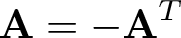 $\textbf{A}=-\textbf{A}^T$.
From the estimate (6.2) $_3$, we have
 \begin{equation*}{1\over ({\varepsilon\delta})^{1/2}}(\partial_\alpha{\mathcal{U}}_{\varepsilon\delta}-(\textbf{R}_{\varepsilon\delta}-\textbf{I}_3)\textbf{e}_\alpha)\to 0\quad\text{strongly in}\ L^2({\omega})^3.\end{equation*}
Besides, the convergences (6.5) lead to
 \begin{equation*}\begin{aligned}
{1\over ({\varepsilon\delta})^{1/2}}(\partial_\alpha{\mathcal{U}}_{\varepsilon\delta}-(\textbf{R}_{\varepsilon\delta}-\textbf{I}_3)\textbf{e}_\alpha)\cdot\textbf{e}_\beta&\rightharpoonup -\textbf{A}\textbf{e}_\alpha\cdot\textbf{e}_\beta\quad&&\text{weakly in } L^2({\omega}),\\
{1\over ({\varepsilon\delta})^{1/2}}(\partial_\alpha{\mathcal{U}}_{\varepsilon\delta}-(\textbf{R}_{\varepsilon\delta}-\textbf{I}_3)\textbf{e}_\alpha)\cdot\textbf{e}_3&\rightharpoonup \partial_\alpha{\mathcal{U}}_3-\textbf{A}\textbf{e}_\alpha\cdot\textbf{e}_3\quad&&\text{weakly in } L^2({\omega}).
\end{aligned}
\end{equation*}
\begin{equation*}\begin{aligned}
{1\over ({\varepsilon\delta})^{1/2}}(\partial_\alpha{\mathcal{U}}_{\varepsilon\delta}-(\textbf{R}_{\varepsilon\delta}-\textbf{I}_3)\textbf{e}_\alpha)\cdot\textbf{e}_\beta&\rightharpoonup -\textbf{A}\textbf{e}_\alpha\cdot\textbf{e}_\beta\quad&&\text{weakly in } L^2({\omega}),\\
{1\over ({\varepsilon\delta})^{1/2}}(\partial_\alpha{\mathcal{U}}_{\varepsilon\delta}-(\textbf{R}_{\varepsilon\delta}-\textbf{I}_3)\textbf{e}_\alpha)\cdot\textbf{e}_3&\rightharpoonup \partial_\alpha{\mathcal{U}}_3-\textbf{A}\textbf{e}_\alpha\cdot\textbf{e}_3\quad&&\text{weakly in } L^2({\omega}).
\end{aligned}
\end{equation*} This gives (6.6) $_2$ and the expression of $\textbf{A}$ given by
 \begin{equation}
\textbf{A}=\left(\begin{matrix}
0&0&-\partial_1{\mathcal{U}}_3\\
0&0&-\partial_2{\mathcal{U}}_3\\
\partial_1{\mathcal{U}}_3 &\partial_2{\mathcal{U}}_3& 0
\end{matrix}\right).
\end{equation}
\begin{equation}
\textbf{A}=\left(\begin{matrix}
0&0&-\partial_1{\mathcal{U}}_3\\
0&0&-\partial_2{\mathcal{U}}_3\\
\partial_1{\mathcal{U}}_3 &\partial_2{\mathcal{U}}_3& 0
\end{matrix}\right).
\end{equation} Observe that due to the estimates (4.16), (4.37) $_4$ and inequality (6.1), we have
 \begin{align}
&\|\textbf{R}^\diamond_{\varepsilon\delta}-\textbf{I}_3\|_{H^1({\omega}_\delta)}\leq C({\varepsilon\delta})^{1/2},\quad\|\textbf{R}_{\varepsilon\delta}-\textbf{R}^\diamond_{\varepsilon\delta}\|_{L^2({\omega}_\delta)}\leq C\varepsilon\sqrt{{\varepsilon\delta}}, \nonumber\\ &\|\partial_\alpha\textbf{R}_{\varepsilon\delta}^\diamond\textbf{e}_{3-\alpha}\|_{L^2({\omega}_\delta)}\leq C{\delta\over \varepsilon}\sqrt{{\varepsilon\delta}},
\end{align}
\begin{align}
&\|\textbf{R}^\diamond_{\varepsilon\delta}-\textbf{I}_3\|_{H^1({\omega}_\delta)}\leq C({\varepsilon\delta})^{1/2},\quad\|\textbf{R}_{\varepsilon\delta}-\textbf{R}^\diamond_{\varepsilon\delta}\|_{L^2({\omega}_\delta)}\leq C\varepsilon\sqrt{{\varepsilon\delta}}, \nonumber\\ &\|\partial_\alpha\textbf{R}_{\varepsilon\delta}^\diamond\textbf{e}_{3-\alpha}\|_{L^2({\omega}_\delta)}\leq C{\delta\over \varepsilon}\sqrt{{\varepsilon\delta}},
\end{align}which imply
 \begin{equation}
\begin{aligned}
{1\over (\varepsilon\delta)^{1/2}}(\textbf{R}^\diamond_{\varepsilon\delta}-\textbf{I}_3)&\rightharpoonup \textbf{A}\quad&&\text{weakly in}\ H^1({\omega})^{3\times 3},\\
{1\over (\varepsilon\delta)^{1/2}}(\textbf{R}_{\varepsilon\delta}-\textbf{I}_3)&\to \textbf{A}\quad&&\text{strongly in}\ L^2({\omega})^{3\times 3}
\end{aligned}
\end{equation}
\begin{equation}
\begin{aligned}
{1\over (\varepsilon\delta)^{1/2}}(\textbf{R}^\diamond_{\varepsilon\delta}-\textbf{I}_3)&\rightharpoonup \textbf{A}\quad&&\text{weakly in}\ H^1({\omega})^{3\times 3},\\
{1\over (\varepsilon\delta)^{1/2}}(\textbf{R}_{\varepsilon\delta}-\textbf{I}_3)&\to \textbf{A}\quad&&\text{strongly in}\ L^2({\omega})^{3\times 3}
\end{aligned}
\end{equation}and  $\textbf{A} \in H^1({\omega})^{3\times 3}$. So, with the expression (6.9) of $\textbf{A}$ using ${\mathcal{U}}_3$, we obtain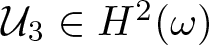 ${\mathcal{U}}_3\in H^2({\omega})$. We also get $\partial_\alpha\textbf{A}\textbf{e}_{3-\alpha}=0$, which imply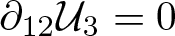 $\partial_{12}{\mathcal{U}}_3=0$. Due to the boundary condition satisfied by ${\mathcal{V}}_{\varepsilon\delta}$ and $\textbf{R}_{\varepsilon\delta}$, we obtained that ${\mathcal{U}}$ also satisfies the corresponding boundary conditions.
Using Lemma 4.8, we obtain
 \begin{equation}
\begin{aligned}
& \|(\textbf{R}^{\diamond}_{\varepsilon\delta}-\textbf{I}_3)\textbf{e}_1-d_1F_{\varepsilon\delta}^{\diamond}\|_{L^2({\omega}_\delta)}+\|(\textbf{R}^{\diamond}_{\varepsilon\delta}-\textbf{I}_3)\textbf{e}_2-d_2G_{\varepsilon\delta}^{\diamond}\|_{L^2({\omega}_\delta)}\leq C\sqrt{{\varepsilon\delta}}\Big({\delta\over \varepsilon}\Big),\\
&\|{\mathcal{U}}^{\diamond}_{{\varepsilon\delta}}-F^{\diamond}_{\varepsilon\delta}-G^{\diamond}_{\varepsilon\delta}\|_{H^1({\omega}_\delta)}\leq C\sqrt{{\varepsilon\delta}}\Big({\delta\over \varepsilon}\Big).
\end{aligned}
\end{equation}
\begin{equation}
\begin{aligned}
& \|(\textbf{R}^{\diamond}_{\varepsilon\delta}-\textbf{I}_3)\textbf{e}_1-d_1F_{\varepsilon\delta}^{\diamond}\|_{L^2({\omega}_\delta)}+\|(\textbf{R}^{\diamond}_{\varepsilon\delta}-\textbf{I}_3)\textbf{e}_2-d_2G_{\varepsilon\delta}^{\diamond}\|_{L^2({\omega}_\delta)}\leq C\sqrt{{\varepsilon\delta}}\Big({\delta\over \varepsilon}\Big),\\
&\|{\mathcal{U}}^{\diamond}_{{\varepsilon\delta}}-F^{\diamond}_{\varepsilon\delta}-G^{\diamond}_{\varepsilon\delta}\|_{H^1({\omega}_\delta)}\leq C\sqrt{{\varepsilon\delta}}\Big({\delta\over \varepsilon}\Big).
\end{aligned}
\end{equation}The convergence (6.7) is direct consequence of (6.12). Observe that
 \begin{equation}
\begin{aligned}
\partial_1{\mathcal{U}}^{\diamond}_{\varepsilon\delta}-(\textbf{R}^\circ_{\varepsilon\delta}-\textbf{I}_3)\textbf{e}_1&=\partial_1{\mathcal{U}}^{\diamond}_{\varepsilon\delta}-d_1F^{\diamond}_{\varepsilon\delta}-(\textbf{R}^{\diamond}_{\varepsilon\delta}-\textbf{I}_3)\textbf{e}_1+d_1F^{\diamond}_{\varepsilon\delta}+(\textbf{R}_{\varepsilon\delta}^{\diamond}-\textbf{R}_{\varepsilon\delta}^\circ)\textbf{e}_1,\\
\partial_2{\mathcal{U}}^{\diamond}_{\varepsilon\delta}-(\textbf{R}^\circ_{\varepsilon\delta}-\textbf{I}_3)\textbf{e}_2&=\partial_2{\mathcal{U}}^{\diamond}_{\varepsilon\delta}-d_2G^{\diamond}_{\varepsilon\delta}-(\textbf{R}^{\diamond}_{\varepsilon\delta}-\textbf{I}_3)\textbf{e}_2+d_2G^{\diamond}_{\varepsilon\delta}+(\textbf{R}_{\varepsilon\delta}^{\diamond}-\textbf{R}_{\varepsilon\delta}^\circ)\textbf{e}_2,
\end{aligned}
\end{equation}
\begin{equation}
\begin{aligned}
\partial_1{\mathcal{U}}^{\diamond}_{\varepsilon\delta}-(\textbf{R}^\circ_{\varepsilon\delta}-\textbf{I}_3)\textbf{e}_1&=\partial_1{\mathcal{U}}^{\diamond}_{\varepsilon\delta}-d_1F^{\diamond}_{\varepsilon\delta}-(\textbf{R}^{\diamond}_{\varepsilon\delta}-\textbf{I}_3)\textbf{e}_1+d_1F^{\diamond}_{\varepsilon\delta}+(\textbf{R}_{\varepsilon\delta}^{\diamond}-\textbf{R}_{\varepsilon\delta}^\circ)\textbf{e}_1,\\
\partial_2{\mathcal{U}}^{\diamond}_{\varepsilon\delta}-(\textbf{R}^\circ_{\varepsilon\delta}-\textbf{I}_3)\textbf{e}_2&=\partial_2{\mathcal{U}}^{\diamond}_{\varepsilon\delta}-d_2G^{\diamond}_{\varepsilon\delta}-(\textbf{R}^{\diamond}_{\varepsilon\delta}-\textbf{I}_3)\textbf{e}_2+d_2G^{\diamond}_{\varepsilon\delta}+(\textbf{R}_{\varepsilon\delta}^{\diamond}-\textbf{R}_{\varepsilon\delta}^\circ)\textbf{e}_2,
\end{aligned}
\end{equation}which together with the estimates (4.17) $_1$, (4.24) $_1$ and the convergences (6.7) give (6.8). Since, using (4.17) $_1$, (4.24) $_1$, and (6.1), we have
 \begin{equation*}{\varepsilon\over \delta}{1\over \sqrt{{\varepsilon\delta}}}\|\partial_{\alpha}{\mathcal{U}}^{\diamond}_{\varepsilon\delta}-(\textbf{R}^\circ_{\varepsilon\delta}-\textbf{I}_3)\textbf{e}_{\alpha}\|_{L^2({\omega}_\delta)}\leq C\varepsilon,\quad {\varepsilon\over \delta}{1\over \sqrt{{\varepsilon\delta}}}\|\textbf{R}^{\diamond}_{\varepsilon\delta}-\textbf{R}^\circ_{\varepsilon\delta}\|_{L^2({\omega}_\delta)}\leq C{\varepsilon^2\over \delta}.\end{equation*}
 The assumption (2.2) $_2$ is needed, so the last terms in (6.13) vanishes in the limit. This completes the proof.
As a consequence of the above lemma, we get the following relation for  ${\mathcal{U}}=({\mathcal{U}}_1,{\mathcal{U}}_2,{\mathcal{U}}_3)$.
Proposition 6.2. The limit displacement  ${\mathcal{U}}=({\mathcal{U}}_1,{\mathcal{U}}_2,{\mathcal{U}}_3)\in H^1_\gamma({\omega})\times H^1_\gamma({\omega})\times H^2_\gamma({\omega})$ satisfies the following
 \begin{equation}
e_{\alpha\beta}({\mathcal{U}})+{1\over 2}\partial_\alpha{\mathcal{U}}_3\partial_\beta{\mathcal{U}}_3=0,\quad \text{a.e. in}\ {\omega}.
\end{equation}
\begin{equation}
e_{\alpha\beta}({\mathcal{U}})+{1\over 2}\partial_\alpha{\mathcal{U}}_3\partial_\beta{\mathcal{U}}_3=0,\quad \text{a.e. in}\ {\omega}.
\end{equation} Moreover, the bending  ${\mathcal{U}}_3$ is given by
 \begin{equation}
\begin{aligned}
&{\mathcal{U}}_3(x_1,x_2)={\mathcal{U}}^{(2)}_3(x_1)+{\mathcal{U}}^{(1)}_3(x_2)\quad \hbox{for a.e. } (x_1,x_2)\in {\omega},\\
& {\mathcal{U}}^{(1)}_3\in H_{(0,l)}^{2}\big((0,L)_{x_2}\big),\quad {\mathcal{U}}^{(2)}_3\in H_{(0,l)}^{2}\big((0,L)_{x_1}\big)\qquad {\mathcal{U}}_3^{(1)}\equiv 0\qquad \hbox{or}\quad {\mathcal{U}}_3^{(2)}\equiv 0.
\end{aligned}
\end{equation}
\begin{equation}
\begin{aligned}
&{\mathcal{U}}_3(x_1,x_2)={\mathcal{U}}^{(2)}_3(x_1)+{\mathcal{U}}^{(1)}_3(x_2)\quad \hbox{for a.e. } (x_1,x_2)\in {\omega},\\
& {\mathcal{U}}^{(1)}_3\in H_{(0,l)}^{2}\big((0,L)_{x_2}\big),\quad {\mathcal{U}}^{(2)}_3\in H_{(0,l)}^{2}\big((0,L)_{x_1}\big)\qquad {\mathcal{U}}_3^{(1)}\equiv 0\qquad \hbox{or}\quad {\mathcal{U}}_3^{(2)}\equiv 0.
\end{aligned}
\end{equation}Furthermore
 \begin{equation}
{\mathcal{U}}_m(x_1,x_2)={\mathcal{U}}_1(x_1)\mathbf{e}_1+{\mathcal{U}}_2(x_2)\mathbf{e}_2\qquad \hbox{for a.e. } (x_1,x_2)\in {\omega}
\end{equation}
\begin{equation}
{\mathcal{U}}_m(x_1,x_2)={\mathcal{U}}_1(x_1)\mathbf{e}_1+{\mathcal{U}}_2(x_2)\mathbf{e}_2\qquad \hbox{for a.e. } (x_1,x_2)\in {\omega}
\end{equation}where  ${\mathcal{U}}_{1}\in H_{(0,l)}^{1}\big((0,L)_{x_1}\big)$ and ${\mathcal{U}}_{2}\in H_{(0,l)}^{1}\big((0,L)_{x_2}\big)$ are given by
 \begin{equation*}d_1{\mathcal{U}}_1=-{1\over 2}\big|d_1 {\mathcal{U}}^{(2)}_3\big|^2,\quad d_2{\mathcal{U}}_2=-{1\over 2}\big|d_2 {\mathcal{U}}^{(1)}_3\big|^2 \qquad \hbox{a.e. in }\ \ (0,L).\end{equation*}
Proof. Step 1: We prove (6.14).
Observe that the identity  $\partial_\alpha {\mathcal{V}}_{\varepsilon\delta} - \textbf{R}_{\varepsilon\delta} \textbf{e}_\alpha = 0=\textbf{R}_{\varepsilon\delta}(\textbf{R}_{\varepsilon\delta})^T-\textbf{I}_3$ holds outside a set of measure at most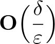 $\displaystyle \textbf{O}\Big({\delta\over \varepsilon}\Big)$ (see (3.2)), then from the estimates (4.38) $_1$, (4.49), (6.1), we deduce the weak convergences
 \begin{equation}
\begin{aligned}
{1\over \varepsilon\delta} \big( \partial_\alpha {\mathcal{U}}_{\varepsilon\delta} - (\textbf{R}_{\varepsilon\delta} - \textbf{I}_3)\textbf{e}_\alpha \big) &\rightharpoonup 0 \quad &&\text{weakly in}\ L^2({\omega})^3,\\
{1\over \varepsilon\delta}\big(\textbf{R}_{\varepsilon\delta}(\textbf{R}_{\varepsilon\delta})^T-\textbf{I}_3\big)& \rightharpoonup 0 \quad&&\text{weakly in}\ L^2({\omega})^{3\times 3}.
\end{aligned}
\end{equation}
\begin{equation}
\begin{aligned}
{1\over \varepsilon\delta} \big( \partial_\alpha {\mathcal{U}}_{\varepsilon\delta} - (\textbf{R}_{\varepsilon\delta} - \textbf{I}_3)\textbf{e}_\alpha \big) &\rightharpoonup 0 \quad &&\text{weakly in}\ L^2({\omega})^3,\\
{1\over \varepsilon\delta}\big(\textbf{R}_{\varepsilon\delta}(\textbf{R}_{\varepsilon\delta})^T-\textbf{I}_3\big)& \rightharpoonup 0 \quad&&\text{weakly in}\ L^2({\omega})^{3\times 3}.
\end{aligned}
\end{equation}Combined with the identity
 \begin{align*}
e_{\alpha\beta}({\mathcal{U}}_{\varepsilon\delta}) - {1\over 2}(\textbf{R}_{\varepsilon\delta} + \textbf{R}_{\varepsilon\delta}^T - 2\textbf{I}_3)\textbf{e}_\alpha \cdot \textbf{e}_\beta &= {1\over 2}(\partial_\alpha {\mathcal{U}}_{\varepsilon\delta} - (\textbf{R}_{\varepsilon\delta} - \textbf{I}_3)\textbf{e}_\alpha) \cdot \textbf{e}_\beta \nonumber\\
&\quad + {1\over 2}(\partial_\beta {\mathcal{U}}_{\varepsilon\delta} - (\textbf{R}_{\varepsilon\delta} - \textbf{I}_3)\textbf{e}_\beta) \cdot \textbf{e}_\alpha.
\end{align*}
\begin{align*}
e_{\alpha\beta}({\mathcal{U}}_{\varepsilon\delta}) - {1\over 2}(\textbf{R}_{\varepsilon\delta} + \textbf{R}_{\varepsilon\delta}^T - 2\textbf{I}_3)\textbf{e}_\alpha \cdot \textbf{e}_\beta &= {1\over 2}(\partial_\alpha {\mathcal{U}}_{\varepsilon\delta} - (\textbf{R}_{\varepsilon\delta} - \textbf{I}_3)\textbf{e}_\alpha) \cdot \textbf{e}_\beta \nonumber\\
&\quad + {1\over 2}(\partial_\beta {\mathcal{U}}_{\varepsilon\delta} - (\textbf{R}_{\varepsilon\delta} - \textbf{I}_3)\textbf{e}_\beta) \cdot \textbf{e}_\alpha.
\end{align*}This implies the weak convergence
 \begin{equation}
{1\over {\varepsilon\delta}} \left[ e_{\alpha\beta}({\mathcal{U}}_{\varepsilon\delta}) - {1\over 2}(\textbf{R}_{\varepsilon\delta} + \textbf{R}_{\varepsilon\delta}^T - 2\textbf{I}_3)\textbf{e}_\alpha \cdot \textbf{e}_\beta \right] \rightharpoonup 0 \quad \text{weakly in}\ L^2({\omega}).
\end{equation}
\begin{equation}
{1\over {\varepsilon\delta}} \left[ e_{\alpha\beta}({\mathcal{U}}_{\varepsilon\delta}) - {1\over 2}(\textbf{R}_{\varepsilon\delta} + \textbf{R}_{\varepsilon\delta}^T - 2\textbf{I}_3)\textbf{e}_\alpha \cdot \textbf{e}_\beta \right] \rightharpoonup 0 \quad \text{weakly in}\ L^2({\omega}).
\end{equation} Using the identity (4.55) along with the convergence (6.17) $_2$ and (6.11) $_2$ gives
 \begin{equation*}{1\over {\varepsilon\delta}}\big(\textbf{R}_{\varepsilon\delta}+(\textbf{R}_{\varepsilon\delta})^T-2\textbf{I}_3\big)\textbf{e}_\alpha\cdot\textbf{e}_\beta \rightharpoonup \textbf{A}^2\textbf{e}_\alpha\cdot\textbf{e}_\beta,\quad\text{weakly in}\ L^2({\omega}),\end{equation*}
which together with (6.5) $_{1}$ imply
 \begin{align*}
&{1\over {\varepsilon\delta}}\Big[e_{\alpha\beta}({\mathcal{U}}_{\varepsilon\delta})-{1\over 2}(\textbf{R}_{\varepsilon\delta}+(\textbf{R}_{\varepsilon\delta})^T-2\textbf{I}_3)\textbf{e}_\alpha\cdot\textbf{e}_\beta\Big]\rightharpoonup e_{\alpha\beta}({\mathcal{U}})-{1\over 2}\textbf{A}^2\textbf{e}_\alpha\cdot\textbf{e}_\beta,\\
&\quad \text{weakly in}\ L^2({\omega}).\end{align*}
\begin{align*}
&{1\over {\varepsilon\delta}}\Big[e_{\alpha\beta}({\mathcal{U}}_{\varepsilon\delta})-{1\over 2}(\textbf{R}_{\varepsilon\delta}+(\textbf{R}_{\varepsilon\delta})^T-2\textbf{I}_3)\textbf{e}_\alpha\cdot\textbf{e}_\beta\Big]\rightharpoonup e_{\alpha\beta}({\mathcal{U}})-{1\over 2}\textbf{A}^2\textbf{e}_\alpha\cdot\textbf{e}_\beta,\\
&\quad \text{weakly in}\ L^2({\omega}).\end{align*} So, from the expression (6.9) of  $\textbf{A}$, we obtain $\textbf{A}^2\textbf{e}_\alpha\cdot\textbf{e}_\beta=-\partial_\alpha{\mathcal{U}}_3\partial_\beta{\mathcal{U}}_3$, which along with (6.18) imply (6.14).
Step 2.
We prove that there exists  ${\mathcal{U}}^{(3-\alpha)}_3\in H_{(0,l)}^{2}\big((0,L)_{x_\alpha}\big)$ such that (6.15) holds.
First, since
 \begin{equation*}{\mathcal{U}}_3 \in H^2_\gamma({\omega})\quad\text{and}\quad \partial_{12}{\mathcal{U}}_3=0\quad\text{a.e. in}\ {\omega},\end{equation*}
there exist  ${\cal F} $ and ${\mathcal{G}}\in H^2(0,L)$ such that
 \begin{equation*}{\mathcal{U}}_3(x_1,x_2)={\cal F}(x_1)+{\mathcal{G}}(x_2)\qquad \hbox{for a.e. } (x_1,x_2)\in {\omega}.\end{equation*}
Besides, we have
 \begin{equation*} {\mathcal{U}}_3=0\quad\hbox{and}\quad \nabla {\mathcal{U}}_3=0\quad \text{a.e. on}\ \gamma.\end{equation*}
This implies
 \begin{equation*}
\begin{aligned}
{\cal F}'(x_1)={\cal F}(x_1)+{\mathcal{G}}(0)=0\quad
{\mathcal{G}}'(x_2)={\mathcal{G}}(x_2)+{\cal F}(0)=0\quad \text{for a.e.}\ (x_1,x_2)\in (0,l)^2.
\end{aligned}
\end{equation*}
\begin{equation*}
\begin{aligned}
{\cal F}'(x_1)={\cal F}(x_1)+{\mathcal{G}}(0)=0\quad
{\mathcal{G}}'(x_2)={\mathcal{G}}(x_2)+{\cal F}(0)=0\quad \text{for a.e.}\ (x_1,x_2)\in (0,l)^2.
\end{aligned}
\end{equation*}So, we obtain (6.15) by setting
 \begin{equation*}{\mathcal{U}}^{(2)}_3={\cal F}+{\mathcal{G}}(0),\qquad {\mathcal{U}}^{(1)}_3={\mathcal{G}}-{\mathcal{G}}(0).\end{equation*}
Step 3. We prove that
 \begin{equation*}
{\mathcal{U}}_3^{(1)}\equiv 0\qquad \hbox{or}\qquad {\mathcal{U}}_3^{(2)}\equiv 0.
\end{equation*}
\begin{equation*}
{\mathcal{U}}_3^{(1)}\equiv 0\qquad \hbox{or}\qquad {\mathcal{U}}_3^{(2)}\equiv 0.
\end{equation*}From (6.14), we have
 \begin{equation*}e_{\alpha\beta}({\mathcal{U}}_m)+{1\over 2}\partial_\alpha{\mathcal{U}}_3\partial_\beta{\mathcal{U}}_3=0,\qquad (\alpha,\beta)\in\{1,2\}^2.\end{equation*}
 We recall that for any membrane displacement belonging to 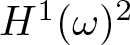 $H^1({\omega})^2$, we have (It is called the Saint–Venant–Kirchhoff compatibility condition.)
 \begin{equation*}
\partial^2_{22}\big(e_{11}({\mathcal{U}}_m)\big)+\partial^2_{11}\big(e_{22}({\mathcal{U}}_m)\big)-2\partial^2_{12}\big(e_{12}({\mathcal{U}}_m)\big)=0 \qquad \hbox{in}\quad \mathcal{D}({\omega}),
\end{equation*}
\begin{equation*}
\partial^2_{22}\big(e_{11}({\mathcal{U}}_m)\big)+\partial^2_{11}\big(e_{22}({\mathcal{U}}_m)\big)-2\partial^2_{12}\big(e_{12}({\mathcal{U}}_m)\big)=0 \qquad \hbox{in}\quad \mathcal{D}({\omega}),
\end{equation*}where  $\mathcal{D}({\omega})$ denotes the space of compactly supported, infinitely differentiable functions on ${\omega}$. So
 \begin{equation*}d^2_{11}{\mathcal{U}}^{(2)}_3(x_1)d^2_{22}{\mathcal{U}}^{(1)}_3(x_2)=0\qquad \hbox{for a.e. } (x_1,x_2)\in{\omega}\end{equation*}
which in turn implies the claim.
Step 4. Below, we determine the membrane displacement  ${\mathcal{U}}_m$.
First, assume 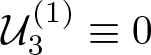 ${\mathcal{U}}^{(1)}_3\equiv 0$. Now, using the equation (6.14) $_1$, we have
 \begin{equation*}\partial_1{\mathcal{U}}_1(x_1,x_2)=-{1\over 2}(d_1{\mathcal{U}}^{(2)}_3)^2(x_1),\quad \partial_2{\mathcal{U}}_2=0,\quad\text{and}\quad \partial_1{\mathcal{U}}_2=-\partial_2{\mathcal{U}}_1.\end{equation*}
 The above conditions imply that there exists 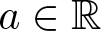 $a\in {\mathbb{R}}$ such that
 \begin{equation*}{\mathcal{U}}_m(x_1,x_2)=\Big(-{1\over 2}\int_0^{x_1} \Big|{d\,{\mathcal{U}}^{(2)}_3\over dt}(t)\Big|^2dt+a x_2\Big)\textbf{e}_1-a x_1\textbf{e}_2\qquad \hbox{for a.e. } (x_1,x_2)\in {\omega}.\end{equation*}
 The boundary conditions imply that  $a=0$. This gives (6.16) in the case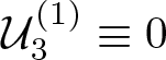 ${\mathcal{U}}^{(1)}_3\equiv 0$. Similarly, we prove the result in the case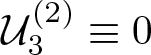 ${\mathcal{U}}^{(2)}_3\equiv 0$. This completes the proof.
6.2. Unfolded limit of the strain tensor
We have the following convergences of the unfolded fields:
Lemma 6.3. There exists  $\overline{v}^{(\alpha)}\in L^2\big({\omega}\times (0,1)_{y_\alpha};H^1\big({\mathfrak{I}}^2\big)\big)^3$ satisfying
 \begin{equation}
\begin{aligned}
\overline{v}^{(1)}(x',y)=0,\quad \text{for a.e.}\ (x',y)\ \text{in}\ {\omega}\times \big(0,1\big)\times \Big\{\pm{1\over 2}\Big\}\times {\mathfrak{I}},\\
\overline{v}^{(2)}(x',y)=0,\quad \text{for a.e.}\ (x',y)\ \text{in}\ {\omega}\times \Big\{\pm{1\over 2}\Big\}\times \big(0,1\big)\times {\mathfrak{I}}.
\end{aligned}
\end{equation}
\begin{equation}
\begin{aligned}
\overline{v}^{(1)}(x',y)=0,\quad \text{for a.e.}\ (x',y)\ \text{in}\ {\omega}\times \big(0,1\big)\times \Big\{\pm{1\over 2}\Big\}\times {\mathfrak{I}},\\
\overline{v}^{(2)}(x',y)=0,\quad \text{for a.e.}\ (x',y)\ \text{in}\ {\omega}\times \Big\{\pm{1\over 2}\Big\}\times \big(0,1\big)\times {\mathfrak{I}}.
\end{aligned}
\end{equation}such that
 \begin{equation}
\begin{aligned}
{1\over {\varepsilon\delta}\sqrt{\varepsilon\delta}}\Pi^{(\alpha)}_{\varepsilon\delta}\big(\overline{v}_{\varepsilon\delta}\big) & \rightharpoonup \overline{v}^{(\alpha)}\quad&&\text{weakly in}\ L^2\big({\omega}\times (0,1)_{y_\alpha};H^1\big({\mathfrak{I}}^2\big)\big)^3,\\
{1\over \varepsilon^2\sqrt{\varepsilon\delta}}\partial_{y_\alpha}\big(\Pi^{(\alpha)}_{\varepsilon\delta}\big(\overline{v}_{\varepsilon\delta}\big)\big) &\rightharpoonup 0\quad&&\text{weakly in}\ L^2({\omega}\times {\mathcal{Y}}_\alpha)^{3}.
\end{aligned}
\end{equation}
\begin{equation}
\begin{aligned}
{1\over {\varepsilon\delta}\sqrt{\varepsilon\delta}}\Pi^{(\alpha)}_{\varepsilon\delta}\big(\overline{v}_{\varepsilon\delta}\big) & \rightharpoonup \overline{v}^{(\alpha)}\quad&&\text{weakly in}\ L^2\big({\omega}\times (0,1)_{y_\alpha};H^1\big({\mathfrak{I}}^2\big)\big)^3,\\
{1\over \varepsilon^2\sqrt{\varepsilon\delta}}\partial_{y_\alpha}\big(\Pi^{(\alpha)}_{\varepsilon\delta}\big(\overline{v}_{\varepsilon\delta}\big)\big) &\rightharpoonup 0\quad&&\text{weakly in}\ L^2({\omega}\times {\mathcal{Y}}_\alpha)^{3}.
\end{aligned}
\end{equation}Moreover,
 \begin{equation}
\begin{aligned}
{1\over \varepsilon}{1\over \sqrt{{\varepsilon\delta}}}\mathcal{T}_{\varepsilon\delta}^{(\alpha)}((\mathbf{R}_{\varepsilon\delta})^T\mathbf{R}_{\varepsilon\delta}-\mathbf{I}_3)& \rightharpoonup 0 &&\text{weakly in}\ L^2({\omega}\times Y_\alpha)^{3\times 3},\\
{1\over \varepsilon}\mathcal{T}_{\varepsilon\delta}^{(\alpha)}\big(\partial_\alpha\mathbf{R}_{\varepsilon\delta}\big)&\rightharpoonup 0 &&\text{weakly in}\ L^2({\omega}\times Y_\alpha)^{3\times 3},\\
{{\delta\over \varepsilon}{1 \over \sqrt{{\varepsilon\delta}}}}\mathcal{T}_{\varepsilon\delta}^{(2)}\big(\partial_1\mathbf{R}_{\varepsilon\delta}\big)&\rightharpoonup \partial_1\mathbf{A} &&\text{weakly in}\ L^2({\omega}\times Y_2)^{3\times 3},\\
{{\delta\over \varepsilon}{1 \over \sqrt{{\varepsilon\delta}}}}\mathcal{T}_{\varepsilon\delta}^{(1)}\big(\partial_2\mathbf{R}_{\varepsilon\delta}\big)&\rightharpoonup \partial_2\mathbf{A} &&\text{weakly in}\ L^2({\omega}\times Y_1)^{3\times 3}.
\end{aligned}
\end{equation}
\begin{equation}
\begin{aligned}
{1\over \varepsilon}{1\over \sqrt{{\varepsilon\delta}}}\mathcal{T}_{\varepsilon\delta}^{(\alpha)}((\mathbf{R}_{\varepsilon\delta})^T\mathbf{R}_{\varepsilon\delta}-\mathbf{I}_3)& \rightharpoonup 0 &&\text{weakly in}\ L^2({\omega}\times Y_\alpha)^{3\times 3},\\
{1\over \varepsilon}\mathcal{T}_{\varepsilon\delta}^{(\alpha)}\big(\partial_\alpha\mathbf{R}_{\varepsilon\delta}\big)&\rightharpoonup 0 &&\text{weakly in}\ L^2({\omega}\times Y_\alpha)^{3\times 3},\\
{{\delta\over \varepsilon}{1 \over \sqrt{{\varepsilon\delta}}}}\mathcal{T}_{\varepsilon\delta}^{(2)}\big(\partial_1\mathbf{R}_{\varepsilon\delta}\big)&\rightharpoonup \partial_1\mathbf{A} &&\text{weakly in}\ L^2({\omega}\times Y_2)^{3\times 3},\\
{{\delta\over \varepsilon}{1 \over \sqrt{{\varepsilon\delta}}}}\mathcal{T}_{\varepsilon\delta}^{(1)}\big(\partial_2\mathbf{R}_{\varepsilon\delta}\big)&\rightharpoonup \partial_2\mathbf{A} &&\text{weakly in}\ L^2({\omega}\times Y_1)^{3\times 3}.
\end{aligned}
\end{equation} Furthermore, there exist  $Z^{(\alpha)},\; {\mathcal{Z}} \in L^2({\omega})^3$ such that
 \begin{equation}
\begin{aligned}
{1\over \varepsilon}{1\over \sqrt{{\varepsilon\delta}}}\mathcal{T}_{\varepsilon\delta}^{(\alpha)}\big(\partial_\alpha{\mathcal{U}}_{\varepsilon\delta}-(\mathbf{R}_{\varepsilon\delta}-\mathbf{I}_3)\mathbf{e}_\alpha\big) &\rightharpoonup 0\\
\text{weakly in}\ L^2({\omega}\times Y_\alpha)^3,\\
{1\over \varepsilon}{1\over \sqrt{{\varepsilon\delta}}}\mathcal{T}_{\varepsilon\delta}^{(2)}\big(\partial_1{\mathcal{U}}_{\varepsilon\delta}-(\mathbf{R}_{\varepsilon\delta}-\mathbf{I}_3)\mathbf{e}_1\big) &\rightharpoonup Z^{(2)}+y_2{\mathcal{Z}}-y_1\partial_1\mathbf{A}\mathbf{e}_1\\
\text{weakly in}\ L^2({\omega}\times Y_2)^3,\\
{1\over \varepsilon}{1\over \sqrt{{\varepsilon\delta}}}\mathcal{T}_{\varepsilon\delta}^{(1)}\big(\partial_2{\mathcal{U}}_{\varepsilon\delta}-(\mathbf{R}_{\varepsilon\delta}-\mathbf{I}_3)\mathbf{e}_2\big) &\rightharpoonup Z^{(1)}-y_2\partial_2\mathbf{A}\mathbf{e}_2+y_1{\mathcal{Z}}\\
\text{weakly in}\ L^2({\omega}\times Y_1)^3.
\end{aligned}
\end{equation}
\begin{equation}
\begin{aligned}
{1\over \varepsilon}{1\over \sqrt{{\varepsilon\delta}}}\mathcal{T}_{\varepsilon\delta}^{(\alpha)}\big(\partial_\alpha{\mathcal{U}}_{\varepsilon\delta}-(\mathbf{R}_{\varepsilon\delta}-\mathbf{I}_3)\mathbf{e}_\alpha\big) &\rightharpoonup 0\\
\text{weakly in}\ L^2({\omega}\times Y_\alpha)^3,\\
{1\over \varepsilon}{1\over \sqrt{{\varepsilon\delta}}}\mathcal{T}_{\varepsilon\delta}^{(2)}\big(\partial_1{\mathcal{U}}_{\varepsilon\delta}-(\mathbf{R}_{\varepsilon\delta}-\mathbf{I}_3)\mathbf{e}_1\big) &\rightharpoonup Z^{(2)}+y_2{\mathcal{Z}}-y_1\partial_1\mathbf{A}\mathbf{e}_1\\
\text{weakly in}\ L^2({\omega}\times Y_2)^3,\\
{1\over \varepsilon}{1\over \sqrt{{\varepsilon\delta}}}\mathcal{T}_{\varepsilon\delta}^{(1)}\big(\partial_2{\mathcal{U}}_{\varepsilon\delta}-(\mathbf{R}_{\varepsilon\delta}-\mathbf{I}_3)\mathbf{e}_2\big) &\rightharpoonup Z^{(1)}-y_2\partial_2\mathbf{A}\mathbf{e}_2+y_1{\mathcal{Z}}\\
\text{weakly in}\ L^2({\omega}\times Y_1)^3.
\end{aligned}
\end{equation}Proof. Step 1: We prove (6.20).
Using the estimates (6.4) and the assumption (2.2), we obtain the convergences (6.20). Observe that (6.20) $_2$ is due to the scaling assumption (2.2) and fact that ((6.4) $_1$)
$_1$)
 \begin{equation*}{1\over \varepsilon^2\sqrt{{\varepsilon\delta}}}\|\Pi^{({\alpha})}_{\varepsilon\delta}(\overline{v}_{\varepsilon\delta})\|_{L^2({\omega}\times {\cal Y}_{\alpha})}\leq C{\delta\over \varepsilon}.\end{equation*}
 In addition, since 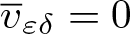 $\overline{v}_{\varepsilon\delta}=0$ a.e. in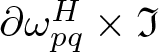 $\partial{\omega}^H_{pq}\times {\mathfrak{I}}$ for all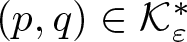 $(p,q)\in{\mathcal{K}}_\varepsilon^*$, passing to the limit gives (6.19).
Step 2: We prove (6.21) $_{2,3,4}$.
Observe that, using the estimates (5.5) and (6.2) $_{6,7}$, we have
 \begin{equation}
\begin{aligned}
&\big\|\mathcal{T}_{\varepsilon\delta}^{(\alpha)}\big((\textbf{R}_{\varepsilon\delta})^T\textbf{R}_{\varepsilon\delta}-\textbf{I}_3\big)\big\|_{L^2({\omega}\times Y_\alpha)}\leq C{\varepsilon\sqrt{{\varepsilon\delta}}},\qquad \big\|\mathcal{T}_{\varepsilon\delta}^{(\alpha)}\big(\nabla \textbf{R}\big)\big\|_{L^2({\omega}\times Y_\alpha)} \leq C{\varepsilon\over \delta}\sqrt{{\varepsilon\delta}}.
\end{aligned}
\end{equation}
\begin{equation}
\begin{aligned}
&\big\|\mathcal{T}_{\varepsilon\delta}^{(\alpha)}\big((\textbf{R}_{\varepsilon\delta})^T\textbf{R}_{\varepsilon\delta}-\textbf{I}_3\big)\big\|_{L^2({\omega}\times Y_\alpha)}\leq C{\varepsilon\sqrt{{\varepsilon\delta}}},\qquad \big\|\mathcal{T}_{\varepsilon\delta}^{(\alpha)}\big(\nabla \textbf{R}\big)\big\|_{L^2({\omega}\times Y_\alpha)} \leq C{\varepsilon\over \delta}\sqrt{{\varepsilon\delta}}.
\end{aligned}
\end{equation} We also have from (4.33) $_{3}$, for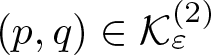 $(p,q)\in {\mathcal{K}}^{(2)}_\varepsilon$
 \begin{equation}
\begin{aligned}
& \partial_1\textbf{R}_{\varepsilon\delta}(p\varepsilon+z_1,q\varepsilon+z_2)={1\over \delta} \big(\textbf{R}_{{\varepsilon\delta},pq}-\textbf{R}_{{\varepsilon\delta},p-1q}\big),\\
& \partial_2\textbf{R}_{\varepsilon\delta}(p\varepsilon+z_1,q\varepsilon+z_2)=0
\end{aligned}
\qquad\forall\,(z_1,z_2)\in{\mathfrak{I}}_\delta\times {\mathfrak{J}}_{\varepsilon\delta}.
\end{equation}
\begin{equation}
\begin{aligned}
& \partial_1\textbf{R}_{\varepsilon\delta}(p\varepsilon+z_1,q\varepsilon+z_2)={1\over \delta} \big(\textbf{R}_{{\varepsilon\delta},pq}-\textbf{R}_{{\varepsilon\delta},p-1q}\big),\\
& \partial_2\textbf{R}_{\varepsilon\delta}(p\varepsilon+z_1,q\varepsilon+z_2)=0
\end{aligned}
\qquad\forall\,(z_1,z_2)\in{\mathfrak{I}}_\delta\times {\mathfrak{J}}_{\varepsilon\delta}.
\end{equation} First, due to the equality (6.24) $_2$, the estimates (4.11) $_2$, (4.45) $_3$, (5.5), and (6.1), we obtain
 \begin{equation*}\big\|\mathcal{T}_{\varepsilon\delta}^{(2)}(\partial_2\textbf{R}_{\varepsilon\delta}) \big\|_{L^2({\omega}\times Y_2)}\leq C\varepsilon.\end{equation*}
 Equality (6.24) $_2$ also implies that the support of the function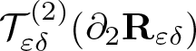 $\mathcal{T}_{\varepsilon\delta}^{(2)}(\partial_2\textbf{R}_{\varepsilon\delta})$ has a measure of order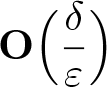 $\displaystyle \textbf{O}\Big({\delta\over \varepsilon}\Big)$. As a consequence, we get (6.21) $_2$ for $\alpha=2$. In the same way, we show the convergence (6.21) $_2$ for $\alpha=1$.
Let  $\phi$ be in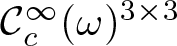 $\mathcal{C}_c^\infty({\omega})^{3\times 3}$. The definition of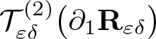 $\mathcal{T}_{\varepsilon\delta}^{(2)}\big(\partial_1\textbf{R}_{\varepsilon\delta}\big)$ and the estimate (6.23) $_2$ lead to
 \begin{equation}\begin{aligned}
\Big|\int_{{\omega}\times Y_2}{{\delta\over \varepsilon}{1 \over \sqrt{{\varepsilon\delta}}}}\mathcal{T}_{\varepsilon\delta}^{(2)}\big(\partial_1\textbf{R}_{\varepsilon\delta}\big):\phi\, dx'dy'-\int_{{\omega}\times Y^{(2)}_{\varepsilon\delta}}{\delta\over \varepsilon}{1 \over \sqrt{{\varepsilon\delta}}}\mathcal{T}_{\varepsilon\delta}^{(2)}\big(\partial_1\textbf{R}_{\varepsilon\delta}\big):\phi\, dx'dy'\Big|\\
\leq
C{\delta\over \varepsilon}\|\phi\|_{L^\infty({\omega}\times Y_2)},
\end{aligned}
\end{equation}
\begin{equation}\begin{aligned}
\Big|\int_{{\omega}\times Y_2}{{\delta\over \varepsilon}{1 \over \sqrt{{\varepsilon\delta}}}}\mathcal{T}_{\varepsilon\delta}^{(2)}\big(\partial_1\textbf{R}_{\varepsilon\delta}\big):\phi\, dx'dy'-\int_{{\omega}\times Y^{(2)}_{\varepsilon\delta}}{\delta\over \varepsilon}{1 \over \sqrt{{\varepsilon\delta}}}\mathcal{T}_{\varepsilon\delta}^{(2)}\big(\partial_1\textbf{R}_{\varepsilon\delta}\big):\phi\, dx'dy'\Big|\\
\leq
C{\delta\over \varepsilon}\|\phi\|_{L^\infty({\omega}\times Y_2)},
\end{aligned}
\end{equation}where  $\displaystyle Y^{(2)}_{\varepsilon\delta}={\mathfrak{I}}\times {1\over \varepsilon}{\mathfrak{J}}_{\varepsilon\delta}=(-{1\over 2},{1\over 2})\times ({\delta\over 2\varepsilon},1-{\delta\over 2\varepsilon})$.
Then, for  $\varepsilon$ small enough and due to (6.24) $_1$, we have
 \begin{equation*}
\begin{aligned}
&\int_{{\omega}\times Y^{(2)}_{\varepsilon\delta}}{\displaystyle{\delta\over \varepsilon}{1 \over \sqrt{{\varepsilon\delta}}}}\mathcal{T}_{\varepsilon\delta}^{(2)}\big(\partial_1\textbf{R}_{\varepsilon\delta}\big):\phi\, dx'dy' \\
& \quad ={1\over \sqrt{{\varepsilon\delta}}}\Big(1-{\delta\over \varepsilon}\Big)\sum_{(p,q)\in {\mathcal{K}}^{(2)}_\varepsilon}\int_{{\omega}_{pq}} {\textbf{R}_{{\varepsilon\delta},pq}-\textbf{R}_{{\varepsilon\delta},p-1q}\over \varepsilon}:\phi\,dx'\\
&\quad ={1\over \sqrt{{\varepsilon\delta}}}\Big(1-{\delta\over \varepsilon}\Big)\sum_{(p,q)\in {\mathcal{K}}^{(2)}_\varepsilon}\int_{{\omega}_{pq}} \big(\textbf{R}_{{\varepsilon\delta},pq}-\textbf{I}_3\big):{\phi - \phi(\cdot+\varepsilon\textbf{e}_1)\over \varepsilon} dx'.
\end{aligned}
\end{equation*}
\begin{equation*}
\begin{aligned}
&\int_{{\omega}\times Y^{(2)}_{\varepsilon\delta}}{\displaystyle{\delta\over \varepsilon}{1 \over \sqrt{{\varepsilon\delta}}}}\mathcal{T}_{\varepsilon\delta}^{(2)}\big(\partial_1\textbf{R}_{\varepsilon\delta}\big):\phi\, dx'dy' \\
& \quad ={1\over \sqrt{{\varepsilon\delta}}}\Big(1-{\delta\over \varepsilon}\Big)\sum_{(p,q)\in {\mathcal{K}}^{(2)}_\varepsilon}\int_{{\omega}_{pq}} {\textbf{R}_{{\varepsilon\delta},pq}-\textbf{R}_{{\varepsilon\delta},p-1q}\over \varepsilon}:\phi\,dx'\\
&\quad ={1\over \sqrt{{\varepsilon\delta}}}\Big(1-{\delta\over \varepsilon}\Big)\sum_{(p,q)\in {\mathcal{K}}^{(2)}_\varepsilon}\int_{{\omega}_{pq}} \big(\textbf{R}_{{\varepsilon\delta},pq}-\textbf{I}_3\big):{\phi - \phi(\cdot+\varepsilon\textbf{e}_1)\over \varepsilon} dx'.
\end{aligned}
\end{equation*} Now, thanks to (4.23), we replace 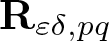 $\textbf{R}_{{\varepsilon\delta},pq}$ by $\textbf{R}^\diamond_{\varepsilon\delta}$. Hence, the above equality and (6.25) yield
 \begin{equation}\begin{aligned}
\Big|\int_{{\omega}\times Y_2}{\delta\over \varepsilon}{1 \over \sqrt{{\varepsilon\delta}}}\mathcal{T}_{\varepsilon\delta}^{(2)}\big(\partial_1\textbf{R}_{\varepsilon\delta}\big):\phi\, dx'dy'\\
\quad -\Big(1-{\delta\over \varepsilon}\Big) \int_{\omega} {1\over \sqrt{{\varepsilon\delta}}}\big(\textbf{R}^\diamond_{\varepsilon\delta}-\textbf{I}_3\big):{\phi - \phi(\cdot+\varepsilon\textbf{e}_1)\over \varepsilon} dx'\Big|\\
\leq C\Big(\varepsilon+{\delta\over \varepsilon}\Big)\|\phi\|_{L^\infty({\omega}\times Y_2)}.
\end{aligned}
\end{equation}
\begin{equation}\begin{aligned}
\Big|\int_{{\omega}\times Y_2}{\delta\over \varepsilon}{1 \over \sqrt{{\varepsilon\delta}}}\mathcal{T}_{\varepsilon\delta}^{(2)}\big(\partial_1\textbf{R}_{\varepsilon\delta}\big):\phi\, dx'dy'\\
\quad -\Big(1-{\delta\over \varepsilon}\Big) \int_{\omega} {1\over \sqrt{{\varepsilon\delta}}}\big(\textbf{R}^\diamond_{\varepsilon\delta}-\textbf{I}_3\big):{\phi - \phi(\cdot+\varepsilon\textbf{e}_1)\over \varepsilon} dx'\Big|\\
\leq C\Big(\varepsilon+{\delta\over \varepsilon}\Big)\|\phi\|_{L^\infty({\omega}\times Y_2)}.
\end{aligned}
\end{equation} Convergence (6.11) $_1$ and the fact that
 \begin{equation*}{\phi - \phi(\cdot+\varepsilon\textbf{e}_1)\over \varepsilon}\longrightarrow -\partial_1\phi\quad \hbox{strongly in }\; L^2({\omega})^{3\times 3}\end{equation*}
imply with (6.26)
 \begin{align*}&\lim_{(\varepsilon,\delta)\to(0,0)}\int_{{\omega}\times Y_2}{\delta\over \varepsilon}{1 \over \sqrt{{\varepsilon\delta}}}\mathcal{T}_{\varepsilon\delta}^{(2)}\big(\partial_1\textbf{R}_{\varepsilon\delta}\big):\phi\, dx'dy'= -\int_{\omega} \textbf{A}:\partial_1\phi\,dx'\\
&=\int_{{\omega} \times Y_2} \partial_1\textbf{A} : \phi\,dx'dy'.\end{align*}
\begin{align*}&\lim_{(\varepsilon,\delta)\to(0,0)}\int_{{\omega}\times Y_2}{\delta\over \varepsilon}{1 \over \sqrt{{\varepsilon\delta}}}\mathcal{T}_{\varepsilon\delta}^{(2)}\big(\partial_1\textbf{R}_{\varepsilon\delta}\big):\phi\, dx'dy'= -\int_{\omega} \textbf{A}:\partial_1\phi\,dx'\\
&=\int_{{\omega} \times Y_2} \partial_1\textbf{A} : \phi\,dx'dy'.\end{align*} Note that, outside to a set of measure 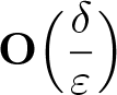 $\displaystyle \textbf{O}\Big({\delta\over \varepsilon}\Big)$, the function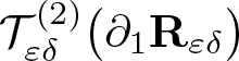 $\mathcal{T}_{\varepsilon\delta}^{(2)}\big(\partial_1\textbf{R}_{\varepsilon\delta}\big)$ does not depend on $y$. This ends the proof of the convergence (6.21) $_3$ for $\alpha=2$. In the same way, we show the convergence (6.21) $_4$ for $\alpha=1$.
Step 3: We prove (6.21) $_1$.
$_1$.
First, we have
 \begin{equation*}
{1\over \varepsilon\sqrt{{\varepsilon\delta}}}\mathcal{T}_{\varepsilon\delta}^{(2)}\big(((\textbf{R}_{\varepsilon\delta})^T\textbf{R}_{\varepsilon\delta}-\textbf{I}_3)\textbf{1}_{Y_2\setminus Y^{(2)}_{\varepsilon\delta}}\big) \rightharpoonup 0 \qquad \text{weakly in } L^2({\omega}\times Y_2)^{3\times 3}.\end{equation*}
\begin{equation*}
{1\over \varepsilon\sqrt{{\varepsilon\delta}}}\mathcal{T}_{\varepsilon\delta}^{(2)}\big(((\textbf{R}_{\varepsilon\delta})^T\textbf{R}_{\varepsilon\delta}-\textbf{I}_3)\textbf{1}_{Y_2\setminus Y^{(2)}_{\varepsilon\delta}}\big) \rightharpoonup 0 \qquad \text{weakly in } L^2({\omega}\times Y_2)^{3\times 3}.\end{equation*} Now, we determine the weak limit of  $\displaystyle {1\over \varepsilon\sqrt{{\varepsilon\delta}}}\mathcal{T}_{\varepsilon\delta}^{(2)}\big(((\textbf{R}_{\varepsilon\delta})^T\textbf{R}_{\varepsilon\delta}-\textbf{I}_3)\textbf{1}_{Y^{(2)}_{\varepsilon\delta}}\big)$. To do that, we consider the field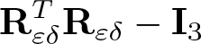 $\textbf{R}^T_{\varepsilon\delta}\textbf{R}_{\varepsilon\delta}-\textbf{I}_3$ in $R^2_{pq}$ for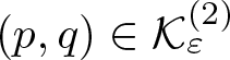 $(p,q)\in{\mathcal{K}}_\varepsilon^{(2)}$. Using (4.33), we have for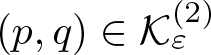 $(p,q)\in{\mathcal{K}}_\varepsilon^{(2)}$ and $(z_1,z_2)\in{\mathfrak{I}}_\delta\times {\mathfrak{J}}_{\varepsilon\delta}$
 \begin{equation*}{\small \begin{aligned}
2\textbf{E}\big(\textbf{R}_{\varepsilon\delta}(p\varepsilon+z_1,q\varepsilon+z_2)\big)&={\delta^2-4x_1^2\over 4\delta^2}\big(\textbf{R}^T_{{\varepsilon\delta},pq}\textbf{R}_{\delta,p-1q}+\textbf{R}^T_{{\varepsilon\delta},p-1q}\textbf{R}_{{\varepsilon\delta},pq}-2\textbf{I}_3\big)\\
&={\delta^2-4x_1^2\over 4\delta^2}\big(\textbf{R}^T_{{\varepsilon\delta},pq}(\textbf{R}_{{\varepsilon\delta},p-1q}-\textbf{R}_{{\varepsilon\delta},pq})\\
&\quad +\textbf{R}^T_{{\varepsilon\delta},p-1q}(\textbf{R}_{{\varepsilon\delta},pq}-\textbf{R}_{{\varepsilon\delta},p-1q})\big).
\end{aligned}
}\end{equation*}
\begin{equation*}{\small \begin{aligned}
2\textbf{E}\big(\textbf{R}_{\varepsilon\delta}(p\varepsilon+z_1,q\varepsilon+z_2)\big)&={\delta^2-4x_1^2\over 4\delta^2}\big(\textbf{R}^T_{{\varepsilon\delta},pq}\textbf{R}_{\delta,p-1q}+\textbf{R}^T_{{\varepsilon\delta},p-1q}\textbf{R}_{{\varepsilon\delta},pq}-2\textbf{I}_3\big)\\
&={\delta^2-4x_1^2\over 4\delta^2}\big(\textbf{R}^T_{{\varepsilon\delta},pq}(\textbf{R}_{{\varepsilon\delta},p-1q}-\textbf{R}_{{\varepsilon\delta},pq})\\
&\quad +\textbf{R}^T_{{\varepsilon\delta},p-1q}(\textbf{R}_{{\varepsilon\delta},pq}-\textbf{R}_{{\varepsilon\delta},p-1q})\big).
\end{aligned}
}\end{equation*}Let us set
 \begin{equation*}\left.\begin{aligned}
\textbf{A}_{\varepsilon\delta}(p\varepsilon+z_1,q\varepsilon+z_2)&=\textbf{R}_{{\varepsilon\delta},pq}-\textbf{R}_{{\varepsilon\delta},p-1q},\\
\textbf{B}_{\varepsilon\delta}(p\varepsilon+z_1,q\varepsilon+z_2)&=\textbf{R}^T_{{\varepsilon\delta},pq},
\end{aligned}
\right\}\quad (p,q)\in{\mathcal{K}}_\varepsilon^{(2)}\ \text{and}\ (z_1,z_2)\in{\mathfrak{I}}_\delta\times {\mathfrak{J}}_{\varepsilon\delta}.\end{equation*}
\begin{equation*}\left.\begin{aligned}
\textbf{A}_{\varepsilon\delta}(p\varepsilon+z_1,q\varepsilon+z_2)&=\textbf{R}_{{\varepsilon\delta},pq}-\textbf{R}_{{\varepsilon\delta},p-1q},\\
\textbf{B}_{\varepsilon\delta}(p\varepsilon+z_1,q\varepsilon+z_2)&=\textbf{R}^T_{{\varepsilon\delta},pq},
\end{aligned}
\right\}\quad (p,q)\in{\mathcal{K}}_\varepsilon^{(2)}\ \text{and}\ (z_1,z_2)\in{\mathfrak{I}}_\delta\times {\mathfrak{J}}_{\varepsilon\delta}.\end{equation*}Then, proceeding as in the previous step with the estimates (4.23), (6.1), and (6.10), we obtain
 \begin{equation*}
\begin{aligned}
{1\over \varepsilon\sqrt{{\varepsilon\delta}}}\mathcal{T}_{\varepsilon\delta}^{(2)}(\textbf{A}_{\varepsilon\delta}\textbf{1}_{Y^{(2)}_{\varepsilon\delta}}) & \rightharpoonup \partial_1\textbf{A}\quad && \text{weakly in}\ L^2({\omega}\times Y_2)^{3\times 3},\\
\mathcal{T}_{\varepsilon\delta}^{(2)}(\textbf{B}_{\varepsilon\delta}\textbf{1}_{Y^{(2)}_{\varepsilon\delta}}) & \to \textbf{I}_3\quad && \text{strongly in}\ L^2({\omega}\times Y_2)^{3\times 3}.
\end{aligned}
\end{equation*}
\begin{equation*}
\begin{aligned}
{1\over \varepsilon\sqrt{{\varepsilon\delta}}}\mathcal{T}_{\varepsilon\delta}^{(2)}(\textbf{A}_{\varepsilon\delta}\textbf{1}_{Y^{(2)}_{\varepsilon\delta}}) & \rightharpoonup \partial_1\textbf{A}\quad && \text{weakly in}\ L^2({\omega}\times Y_2)^{3\times 3},\\
\mathcal{T}_{\varepsilon\delta}^{(2)}(\textbf{B}_{\varepsilon\delta}\textbf{1}_{Y^{(2)}_{\varepsilon\delta}}) & \to \textbf{I}_3\quad && \text{strongly in}\ L^2({\omega}\times Y_2)^{3\times 3}.
\end{aligned}
\end{equation*}Finally, we obtain
 \begin{align*}
&{1\over \varepsilon\sqrt{{\varepsilon\delta}}}\mathcal{T}_{\varepsilon\delta}^{(2)}\big(((\textbf{R}_{\varepsilon\delta})^T\textbf{R}_{\varepsilon\delta}-\textbf{I}_3)\textbf{1}_{Y^{(2)}_{\varepsilon\delta}}\big) \rightharpoonup \big(-\partial_1\textbf{A}+\partial_1\textbf{A}\big){1-4y^2_1\over 4}=0 \nonumber\\
&\quad \text{weakly in}\ L^1({\omega}\times Y_2)^{3\times 3}.\end{align*}
\begin{align*}
&{1\over \varepsilon\sqrt{{\varepsilon\delta}}}\mathcal{T}_{\varepsilon\delta}^{(2)}\big(((\textbf{R}_{\varepsilon\delta})^T\textbf{R}_{\varepsilon\delta}-\textbf{I}_3)\textbf{1}_{Y^{(2)}_{\varepsilon\delta}}\big) \rightharpoonup \big(-\partial_1\textbf{A}+\partial_1\textbf{A}\big){1-4y^2_1\over 4}=0 \nonumber\\
&\quad \text{weakly in}\ L^1({\omega}\times Y_2)^{3\times 3}.\end{align*} The estimate (6.23) $_1$ and the above convergence lead to (6.21) $_1$ for $\alpha=2$. The case $\alpha=1$ is similar.
Step 4: We prove the convergences (6.22).
From the estimate (6.2) $_3$ and the properties of $\mathcal{T}_{\varepsilon\delta}^{(\alpha)}$, we obtain
 \begin{equation*}
\|\mathcal{T}_{\varepsilon\delta}^{(\alpha)}\big(\partial_\beta{\mathcal{U}}_{\varepsilon\delta}-(\textbf{R}_{\varepsilon\delta}-\textbf{I}_3)\textbf{e}_\beta\big)\|_{L^2({\omega}\times Y_\alpha)}\leq C\varepsilon\sqrt{{\varepsilon\delta}}.
\end{equation*}
\begin{equation*}
\|\mathcal{T}_{\varepsilon\delta}^{(\alpha)}\big(\partial_\beta{\mathcal{U}}_{\varepsilon\delta}-(\textbf{R}_{\varepsilon\delta}-\textbf{I}_3)\textbf{e}_\beta\big)\|_{L^2({\omega}\times Y_\alpha)}\leq C\varepsilon\sqrt{{\varepsilon\delta}}.
\end{equation*} As in the previous steps, we only have to consider  $\partial_\beta{\mathcal{U}}_{\varepsilon\delta}-(\textbf{R}_{\varepsilon\delta}-\textbf{I}_3)\textbf{e}_\beta$ in the rectangles $R^2_{pq}$ for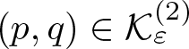 $(p,q)\in{\mathcal{K}}_\varepsilon^{(2)}$.
We recall from Step 3 of Lemma 4.9, for a.e.  $(z_1,z_2)\in{\mathfrak{I}}_\delta\times {\mathfrak{J}}_{\varepsilon\delta}$ and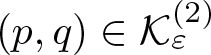 $(p,q)\in {\mathcal{K}}^{(2)}_\varepsilon$
 \begin{equation*}
\begin{aligned}
\big(\partial_2{\mathcal{V}}_{\varepsilon\delta}-\textbf{R}_{\varepsilon\delta}\textbf{e}_2\big)(p\varepsilon+z_1,q\varepsilon+z_2)&=0,\\
\big(\partial_1{\mathcal{V}}_{\varepsilon\delta}-\textbf{R}_{\varepsilon\delta}\textbf{e}_1\big)(p\varepsilon+z_1,q\varepsilon+z_2)
&={1\over \delta}\big(\textbf{a}_{{\varepsilon\delta},pq}-\textbf{a}_{{\varepsilon\delta},p-1q}-\varepsilon\textbf{R}_{{\varepsilon\delta},p-1q}\textbf{e}_1\big)\\
&+{z_2\over \delta}(\textbf{R}_{{\varepsilon\delta},pq}-\textbf{R}_{{\varepsilon\delta},p-1q})\textbf{e}_2\\
&-{z_1\over \delta}(\textbf{R}_{{\varepsilon\delta},pq}-\textbf{R}_{{\varepsilon\delta},p-1q})\textbf{e}_1.
\end{aligned}
\end{equation*}
\begin{equation*}
\begin{aligned}
\big(\partial_2{\mathcal{V}}_{\varepsilon\delta}-\textbf{R}_{\varepsilon\delta}\textbf{e}_2\big)(p\varepsilon+z_1,q\varepsilon+z_2)&=0,\\
\big(\partial_1{\mathcal{V}}_{\varepsilon\delta}-\textbf{R}_{\varepsilon\delta}\textbf{e}_1\big)(p\varepsilon+z_1,q\varepsilon+z_2)
&={1\over \delta}\big(\textbf{a}_{{\varepsilon\delta},pq}-\textbf{a}_{{\varepsilon\delta},p-1q}-\varepsilon\textbf{R}_{{\varepsilon\delta},p-1q}\textbf{e}_1\big)\\
&+{z_2\over \delta}(\textbf{R}_{{\varepsilon\delta},pq}-\textbf{R}_{{\varepsilon\delta},p-1q})\textbf{e}_2\\
&-{z_1\over \delta}(\textbf{R}_{{\varepsilon\delta},pq}-\textbf{R}_{{\varepsilon\delta},p-1q})\textbf{e}_1.
\end{aligned}
\end{equation*} Proceeding as in the previous steps, the above expression give (6.22) $_1$ for $\alpha=2$. Then, using the estimates (4.11) $_{1,3,5}$ and (6.1), we obtain the convergence (6.22) $_2$ with ${\mathcal{Z}}^{(2)}\in L^2({\omega})^3$. The case $\alpha=1$ is similar, with ${\mathcal{Z}}^{(1)}\in L^2({\omega})^3$. Using the estimates (4.23), (4.29) with (6.1) and the convergences (6.7) $_{1,2}$ give
 \begin{equation*}{\mathcal{Z}}^{(1)}=\partial_2{\mathcal{R}}^{(1)},\quad \text{in}\ {\omega},\quad {\mathcal{Z}}^{(2)}=\partial_1{\mathcal{R}}^{(2)},\quad \text{in}\ {\omega},\end{equation*}
which together with (6.8) imply  ${\mathcal{Z}}^{(1)}={\mathcal{Z}}^{(2)}=\partial_{12}U$. Since $(\textbf{R}^\diamond_{\varepsilon\delta}-\textbf{I}_3)(-{\delta\over 2},\cdot)\textbf{e}_2$ is independent of $z_1$. Similarly $(\textbf{R}^\diamond_{\varepsilon\delta}-\textbf{I}_3)(\cdot,-{\delta\over 2})\textbf{e}_1$ is independent of $z_2$. This completes the proof.
Observe that, we have the following identity
 \begin{align}
\textbf{E}(\nabla v_{\varepsilon\delta})&=(\nabla v_{\varepsilon\delta})^T(\nabla v_{\varepsilon\delta})-\textbf{I}_3= (\nabla v_{\varepsilon\delta}-\textbf{R}_{\varepsilon\delta})^T\nabla v_{\varepsilon\delta} \nonumber\\
&\quad +(\textbf{R}_{\varepsilon\delta})^T(\nabla v_{\varepsilon\delta}-\textbf{R}_{\varepsilon\delta})+ \big((\textbf{R}_{\varepsilon\delta})^T\textbf{R}_{\varepsilon\delta}-\textbf{I}_3\big).
\end{align}
\begin{align}
\textbf{E}(\nabla v_{\varepsilon\delta})&=(\nabla v_{\varepsilon\delta})^T(\nabla v_{\varepsilon\delta})-\textbf{I}_3= (\nabla v_{\varepsilon\delta}-\textbf{R}_{\varepsilon\delta})^T\nabla v_{\varepsilon\delta} \nonumber\\
&\quad +(\textbf{R}_{\varepsilon\delta})^T(\nabla v_{\varepsilon\delta}-\textbf{R}_{\varepsilon\delta})+ \big((\textbf{R}_{\varepsilon\delta})^T\textbf{R}_{\varepsilon\delta}-\textbf{I}_3\big).
\end{align} In the  $\textbf{e}_\alpha$-direction, for a.e.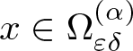 $x\in \Omega^{(\alpha)}_{\varepsilon\delta}$, we have using the decomposition (4.35)
 \begin{equation}
\begin{aligned}
\big(\nabla v_{\varepsilon\delta}(x)-\textbf{R}_{\varepsilon\delta}(x')\big)\textbf{e}_\beta&=\big(\partial_\beta{\mathcal{U}}_{\varepsilon\delta}-(\textbf{R}_{\varepsilon\delta}-\textbf{I}_3)\textbf{e}_\beta\big)(x')+x_3\partial_\beta\textbf{R}_{\varepsilon\delta}(x')\textbf{e}_3+\partial_\beta\overline{v}_{\varepsilon\delta}(x),\\
\big(\nabla v_{\varepsilon\delta}(x)-\textbf{R}_{\varepsilon\delta}(x')\big)\textbf{e}_3&=\partial_3\overline{v}_{\varepsilon\delta}(x).
\end{aligned}
\end{equation}
\begin{equation}
\begin{aligned}
\big(\nabla v_{\varepsilon\delta}(x)-\textbf{R}_{\varepsilon\delta}(x')\big)\textbf{e}_\beta&=\big(\partial_\beta{\mathcal{U}}_{\varepsilon\delta}-(\textbf{R}_{\varepsilon\delta}-\textbf{I}_3)\textbf{e}_\beta\big)(x')+x_3\partial_\beta\textbf{R}_{\varepsilon\delta}(x')\textbf{e}_3+\partial_\beta\overline{v}_{\varepsilon\delta}(x),\\
\big(\nabla v_{\varepsilon\delta}(x)-\textbf{R}_{\varepsilon\delta}(x')\big)\textbf{e}_3&=\partial_3\overline{v}_{\varepsilon\delta}(x).
\end{aligned}
\end{equation}In the following theorem, we present the limit of the Green–St. Venant deformation tensor.
Theorem 6.4. We have the following convergences
 \begin{equation}
\left.\begin{aligned}
{1\over 2\varepsilon\sqrt{{\varepsilon\delta}}}\Pi^{(1)}_{\varepsilon\delta}\big((\nabla v_{\varepsilon\delta})^T(\nabla v_{\varepsilon\delta})-\textbf{I}_3\big) &\rightharpoonup E^{(1)}\big({\mathcal{U}}^{(1)}_3,\widehat {v}^{(1)}\big)\quad\text{weakly in }\; L^1({\omega}\times {\mathcal{Y}}_1)^{3\times 3},\\
{1\over 2\varepsilon\sqrt{{\varepsilon\delta}}}\Pi^{(2)}_{\varepsilon\delta}\big((\nabla v_{\varepsilon\delta})^T(\nabla v_{\varepsilon\delta})-\textbf{I}_3\big) &\rightharpoonup E^{(2)}\big({\mathcal{U}}^{(2)}_3,\widehat {v}^{(2)}\big)\quad\text{weakly in }\; L^1({\omega}\times {\mathcal{Y}}_2)^{3\times 3},
\end{aligned}
\right.
\end{equation}
\begin{equation}
\left.\begin{aligned}
{1\over 2\varepsilon\sqrt{{\varepsilon\delta}}}\Pi^{(1)}_{\varepsilon\delta}\big((\nabla v_{\varepsilon\delta})^T(\nabla v_{\varepsilon\delta})-\textbf{I}_3\big) &\rightharpoonup E^{(1)}\big({\mathcal{U}}^{(1)}_3,\widehat {v}^{(1)}\big)\quad\text{weakly in }\; L^1({\omega}\times {\mathcal{Y}}_1)^{3\times 3},\\
{1\over 2\varepsilon\sqrt{{\varepsilon\delta}}}\Pi^{(2)}_{\varepsilon\delta}\big((\nabla v_{\varepsilon\delta})^T(\nabla v_{\varepsilon\delta})-\textbf{I}_3\big) &\rightharpoonup E^{(2)}\big({\mathcal{U}}^{(2)}_3,\widehat {v}^{(2)}\big)\quad\text{weakly in }\; L^1({\omega}\times {\mathcal{Y}}_2)^{3\times 3},
\end{aligned}
\right.
\end{equation}where the symmetric matrices 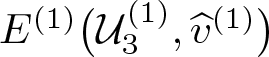 $E^{(1)}\big({\mathcal{U}}^{(1)}_3,\widehat {v}^{(1)}\big)$,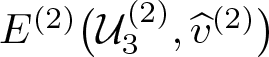 $E^{(2)}\big({\mathcal{U}}^{(2)}_3,\widehat {v}^{(2)}\big)$ are given by
 \begin{equation*}
\begin{aligned}
E^{(1)}\big({\mathcal{U}}^{(1)}_3,\widehat {v}^{(1)}\big)=\left(\begin{matrix}
\displaystyle 0& * &\displaystyle *\\[2mm]
\displaystyle{1\over 2}\partial_{y_2}\widehat {v}^{(1)}_1 & \displaystyle e_{22,y}\big(\widehat {v}^{(1)}\big) -y_3 d^2_{22}{\mathcal{U}}^{(1)}_3 & * \\[2mm]
\displaystyle{1\over 2} \partial_{y_3}\widehat {v}^{(1)}_1 & \displaystyle e_{23,y}\big(\widehat {v}^{(1)}\big)- {y_2\over 2} d^2_{22}{\mathcal{U}}^{(1)}_3 & \displaystyle e_{33,y}\big(\widehat {v}^{(1)}\big)
\end{matrix}\right)
\end{aligned}
\end{equation*}
\begin{equation*}
\begin{aligned}
E^{(1)}\big({\mathcal{U}}^{(1)}_3,\widehat {v}^{(1)}\big)=\left(\begin{matrix}
\displaystyle 0& * &\displaystyle *\\[2mm]
\displaystyle{1\over 2}\partial_{y_2}\widehat {v}^{(1)}_1 & \displaystyle e_{22,y}\big(\widehat {v}^{(1)}\big) -y_3 d^2_{22}{\mathcal{U}}^{(1)}_3 & * \\[2mm]
\displaystyle{1\over 2} \partial_{y_3}\widehat {v}^{(1)}_1 & \displaystyle e_{23,y}\big(\widehat {v}^{(1)}\big)- {y_2\over 2} d^2_{22}{\mathcal{U}}^{(1)}_3 & \displaystyle e_{33,y}\big(\widehat {v}^{(1)}\big)
\end{matrix}\right)
\end{aligned}
\end{equation*}and
 \begin{equation*}
E^{(2)}\big({\mathcal{U}}^{(2)}_3,\widehat {v}^{(2)}\big)=\left(\begin{matrix}
\displaystyle e_{11,y}(\widehat {v}^{(2)})-y_3d^2_{11}{\mathcal{U}}^{(2)}_3 & \displaystyle * &\displaystyle *\\
\displaystyle {1\over 2}\partial_{y_1}\widehat {v}^{(2)}_2 & 0 & *\\
\displaystyle e_{13,y}(\widehat {v}^{(2)}) - {y_1\over 2} d^2_{11}{\mathcal{U}}^{(2)}_3& \displaystyle {1\over 2} \partial_{y_3}\widehat {v}^{(2)}_2 & \displaystyle e_{33,y}(\widehat {v}^{(2)})
\end{matrix}\right),
\end{equation*}
\begin{equation*}
E^{(2)}\big({\mathcal{U}}^{(2)}_3,\widehat {v}^{(2)}\big)=\left(\begin{matrix}
\displaystyle e_{11,y}(\widehat {v}^{(2)})-y_3d^2_{11}{\mathcal{U}}^{(2)}_3 & \displaystyle * &\displaystyle *\\
\displaystyle {1\over 2}\partial_{y_1}\widehat {v}^{(2)}_2 & 0 & *\\
\displaystyle e_{13,y}(\widehat {v}^{(2)}) - {y_1\over 2} d^2_{11}{\mathcal{U}}^{(2)}_3& \displaystyle {1\over 2} \partial_{y_3}\widehat {v}^{(2)}_2 & \displaystyle e_{33,y}(\widehat {v}^{(2)})
\end{matrix}\right),
\end{equation*}with  $\overline{v}^{(\alpha)}\in L^2\big({\omega}\times (0,1)_{y_\alpha};H^1\big({\mathfrak{I}}^2\big)\big)^3$ satisfying (6.19) and $Z^{(\alpha)}, {\mathcal{Z}}\in L^2({\omega})^3$, from Lemma 6.3 such that
 \begin{equation}
\widehat v^{(2)}=\overline{v}^{(2)}+y_1 Z^{(2)}+y_1y_2 {\mathcal{Z}},\qquad \widehat v^{(1)}=\overline{v}^{(1)}+y_2 Z^{(1)}+y_1 y_2 {\mathcal{Z}}.
\end{equation}
\begin{equation}
\widehat v^{(2)}=\overline{v}^{(2)}+y_1 Z^{(2)}+y_1y_2 {\mathcal{Z}},\qquad \widehat v^{(1)}=\overline{v}^{(1)}+y_2 Z^{(1)}+y_1 y_2 {\mathcal{Z}}.
\end{equation}Proof. As a consequence of the convergences (6.20) and (6.22)–(6.21), we obtain the following weak convergences in 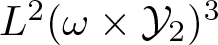 $L^2({\omega}\times {\mathcal{Y}}_2)^3$:
 \begin{equation*}
\begin{aligned}
{1\over \varepsilon\sqrt{{\varepsilon\delta}}}\Pi_{\varepsilon\delta}^{(2)}\big(\nabla v_{\varepsilon\delta}-\textbf{R}_{\varepsilon\delta}\big)\textbf{e}_1\big)&\rightharpoonup Z^{(2)}+y_2{\mathcal{Z}}-y_1\partial_1\textbf{A}\textbf{e}_1+y_3\partial_1\textbf{A}\textbf{e}_3+\partial_{y_1}\overline{v}^{(2)},\\
{1\over \varepsilon\sqrt{{\varepsilon\delta}}}\Pi_{\varepsilon\delta}^{(2)}\big(\nabla v_{\varepsilon\delta}-\textbf{R}_{\varepsilon\delta}\big)\textbf{e}_2\big) &\rightharpoonup 0,\\
{1\over \varepsilon\sqrt{{\varepsilon\delta}}}\Pi_{\varepsilon\delta}^{(2)}\big(\nabla v_{\varepsilon\delta}-\textbf{R}_{\varepsilon\delta}\big)\textbf{e}_3\big)&\rightharpoonup \partial_{y_3}\overline{v}^{(2)}.
\end{aligned}
\end{equation*}
\begin{equation*}
\begin{aligned}
{1\over \varepsilon\sqrt{{\varepsilon\delta}}}\Pi_{\varepsilon\delta}^{(2)}\big(\nabla v_{\varepsilon\delta}-\textbf{R}_{\varepsilon\delta}\big)\textbf{e}_1\big)&\rightharpoonup Z^{(2)}+y_2{\mathcal{Z}}-y_1\partial_1\textbf{A}\textbf{e}_1+y_3\partial_1\textbf{A}\textbf{e}_3+\partial_{y_1}\overline{v}^{(2)},\\
{1\over \varepsilon\sqrt{{\varepsilon\delta}}}\Pi_{\varepsilon\delta}^{(2)}\big(\nabla v_{\varepsilon\delta}-\textbf{R}_{\varepsilon\delta}\big)\textbf{e}_2\big) &\rightharpoonup 0,\\
{1\over \varepsilon\sqrt{{\varepsilon\delta}}}\Pi_{\varepsilon\delta}^{(2)}\big(\nabla v_{\varepsilon\delta}-\textbf{R}_{\varepsilon\delta}\big)\textbf{e}_3\big)&\rightharpoonup \partial_{y_3}\overline{v}^{(2)}.
\end{aligned}
\end{equation*} The above convergences and (6.21) $_1$ give the following
 \begin{align*}
{1\over \varepsilon\sqrt{{\varepsilon\delta}}}\Pi^{(2)}\big(\textbf{E}(v_{\varepsilon\delta})\big) & \rightharpoonup \left(\begin{matrix}
Z^{(2)}_1+y_2{\mathcal{Z}}_1 & * & *\\
{1\over 2}(Z^{(2)}_2+y_2{\mathcal{Z}}_2)& 0& *\\
{1\over 2}(Z_3^{(2)}+y_2{\mathcal{Z}}_3)&0&0
\end{matrix}\right)+E^{(2)}({\cal U}_3^{(2)},\overline{v}^{(2)}), \nonumber\\
&\quad \text{weakly in}\ L^1({\omega}\times {\cal Y}_2)^{3\times 3}.
\end{align*}
\begin{align*}
{1\over \varepsilon\sqrt{{\varepsilon\delta}}}\Pi^{(2)}\big(\textbf{E}(v_{\varepsilon\delta})\big) & \rightharpoonup \left(\begin{matrix}
Z^{(2)}_1+y_2{\mathcal{Z}}_1 & * & *\\
{1\over 2}(Z^{(2)}_2+y_2{\mathcal{Z}}_2)& 0& *\\
{1\over 2}(Z_3^{(2)}+y_2{\mathcal{Z}}_3)&0&0
\end{matrix}\right)+E^{(2)}({\cal U}_3^{(2)},\overline{v}^{(2)}), \nonumber\\
&\quad \text{weakly in}\ L^1({\omega}\times {\cal Y}_2)^{3\times 3}.
\end{align*} Then, setting as in (6.30) $_1$ gives (6.29) $_2$. Similarly, we show (6.29) $_1$.
$_1$.
7. Rescaled minimization problem
This section is devoted to the derivation and analysis of the limiting problem. Using the decomposition of deformations and the rescaled unfolding operators developed in earlier sections, we characterize the asymptotic behaviour of the elastic energy through a form of  $\Gamma$-convergence. We establish the existence of a minimizers for the limiting functional. The resulting limit model is of constrained Kármán type and includes a non-standard isometry constraint on the in-plane strains. We also construct a recovery sequence to complete the convergence analysis.
7.1. Limit minimization problem as
$(\varepsilon,\delta)\to(0,0)$

We define the limit microscopic displacement space as
 \begin{equation}
\begin{aligned}
&\textbf{L}^2\big((0,1)_{y_1};H^1\big({\mathfrak{I}}^2\big)\big)^3 \\
&\quad = \Big\{\widehat {v}^{(1)}\in L^2\big((0,1)_{y_1};H^1({\mathfrak{I}}^2)\big)^3\;|\; \widehat v^{(1)}=\overline{v}^{(1)}+y_2 Z^{(1)}+y_1y_2 {\mathcal{Z}},\\
&\quad Z^{(1)},\; {\mathcal{Z}}\in {\mathbb{R}}^3\quad \text{with}\ \overline{v}^{(1)}\ \text{satisfying (7.2)}_1\Big\},\\
&\quad \textbf{L}^2\big((0,1)_{y_2};H^1\big({\mathfrak{I}}^2\big)\big)^3 \\
& \quad =\Big\{\widehat v^{(2)}\in L^2\big((0,1)_{y_2}; H^1({\mathfrak{I}}^2)\big)^3\,|\,\overline{v}^{(2)}=\overline{v}^{(2)}+y_1 Z^{(2)}+y_1y_2 {\mathcal{Z}},\\
&\quad Z^{(2)},\; {\mathcal{Z}}\in{\mathbb{R}}^3\quad \text{with}\ \overline{v}^{(2)}\ \text{satisfying (7.2)}_2\Big\},
\end{aligned}
\end{equation}
\begin{equation}
\begin{aligned}
&\textbf{L}^2\big((0,1)_{y_1};H^1\big({\mathfrak{I}}^2\big)\big)^3 \\
&\quad = \Big\{\widehat {v}^{(1)}\in L^2\big((0,1)_{y_1};H^1({\mathfrak{I}}^2)\big)^3\;|\; \widehat v^{(1)}=\overline{v}^{(1)}+y_2 Z^{(1)}+y_1y_2 {\mathcal{Z}},\\
&\quad Z^{(1)},\; {\mathcal{Z}}\in {\mathbb{R}}^3\quad \text{with}\ \overline{v}^{(1)}\ \text{satisfying (7.2)}_1\Big\},\\
&\quad \textbf{L}^2\big((0,1)_{y_2};H^1\big({\mathfrak{I}}^2\big)\big)^3 \\
& \quad =\Big\{\widehat v^{(2)}\in L^2\big((0,1)_{y_2}; H^1({\mathfrak{I}}^2)\big)^3\,|\,\overline{v}^{(2)}=\overline{v}^{(2)}+y_1 Z^{(2)}+y_1y_2 {\mathcal{Z}},\\
&\quad Z^{(2)},\; {\mathcal{Z}}\in{\mathbb{R}}^3\quad \text{with}\ \overline{v}^{(2)}\ \text{satisfying (7.2)}_2\Big\},
\end{aligned}
\end{equation}with
 \begin{equation}
\overline{v}^{(1)}=0,\quad\text{a.e. on}\ (0,1)\times \{\pm{1\over 2}\}\times {\mathfrak{I}},\quad \overline{v}^{(2)}=0,\quad\text{a.e. on}\ \{\pm{1\over 2}\}\times (0,1)\times {\mathfrak{I}}.
\end{equation}
\begin{equation}
\overline{v}^{(1)}=0,\quad\text{a.e. on}\ (0,1)\times \{\pm{1\over 2}\}\times {\mathfrak{I}},\quad \overline{v}^{(2)}=0,\quad\text{a.e. on}\ \{\pm{1\over 2}\}\times (0,1)\times {\mathfrak{I}}.
\end{equation}We define the set of limit displacements as
 \begin{equation*}
{\mathbb{D}}\doteq {\mathbb{D}}_0\times L^2\big({\omega}; \textbf{L}^2\big((0,1)_{y_1};H^1\big({\mathfrak{I}}^2\big)\big)^3\big)\times L^2\big({\omega}; \textbf{L}^2\big((0,1)_{y_2};H^1\big({\mathfrak{I}}^2\big)\big)^3\big),
\end{equation*}
\begin{equation*}
{\mathbb{D}}\doteq {\mathbb{D}}_0\times L^2\big({\omega}; \textbf{L}^2\big((0,1)_{y_1};H^1\big({\mathfrak{I}}^2\big)\big)^3\big)\times L^2\big({\omega}; \textbf{L}^2\big((0,1)_{y_2};H^1\big({\mathfrak{I}}^2\big)\big)^3\big),
\end{equation*}where the set of macroscopic displacements is given by
 \begin{align*}{\mathbb{D}}_0&\doteq\left\{{\mathcal{U}}_3\in H^2({\omega})\,|\,{\mathcal{U}}_3(x')={\mathcal{U}}_3^{(2)}(x_1)+{\mathcal{U}}_3^{(1)}(x_2), \right.\nonumber\\
&\quad \left.\text{with}\; {\mathcal{U}}_3^{(3-\alpha)}\in H_{(0,l)}^{2}\big((0,L)_{x_\alpha}\big),\;\text{and}\; {\mathcal{U}}_3^{(1)}{\mathcal{U}}_3^{(2)}=0 \right\}.\end{align*}
\begin{align*}{\mathbb{D}}_0&\doteq\left\{{\mathcal{U}}_3\in H^2({\omega})\,|\,{\mathcal{U}}_3(x')={\mathcal{U}}_3^{(2)}(x_1)+{\mathcal{U}}_3^{(1)}(x_2), \right.\nonumber\\
&\quad \left.\text{with}\; {\mathcal{U}}_3^{(3-\alpha)}\in H_{(0,l)}^{2}\big((0,L)_{x_\alpha}\big),\;\text{and}\; {\mathcal{U}}_3^{(1)}{\mathcal{U}}_3^{(2)}=0 \right\}.\end{align*} Now, we define the limit minimization energy. For that we assume the following: there exists  ${\mathbb{A}}^{(\alpha)}_{ijkl}\in L^\infty\big({\mathcal{Y}}_\alpha\big)^{6\times 6}$, for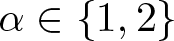 $\alpha\in\{1,2\}$ such that
 \begin{equation}
\Pi^{(\alpha)}_{\varepsilon\delta}({\mathbb{A}}_{\varepsilon\delta}) (x',y)\to {\mathbb{A}}^{(\alpha)}(y) \qquad \hbox{a.e. in } {\omega}\times {\mathcal{Y}}_\alpha,
\end{equation}
\begin{equation}
\Pi^{(\alpha)}_{\varepsilon\delta}({\mathbb{A}}_{\varepsilon\delta}) (x',y)\to {\mathbb{A}}^{(\alpha)}(y) \qquad \hbox{a.e. in } {\omega}\times {\mathcal{Y}}_\alpha,
\end{equation} Observe that  ${\mathbb{A}}^{(\alpha)}$ satisfies the following for a.e.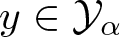 $y\in {\mathcal{Y}}_\alpha$ and for all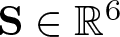 $\textbf{S}\in{\mathbb{R}}^6$
 \begin{equation}
\begin{aligned}
&[{\mathbb{A}}^{(\alpha)}(y)]^T=[{\mathbb{A}}^{(\alpha)}(y)],\\
&\textbf{S}^T{\mathbb{A}}^{(\alpha)}(y)\textbf{S}=\lim_{(\varepsilon,\delta)\to(0,0)}\textbf{S}^T\Pi_{\varepsilon\delta}^{(\alpha)}({\mathbb{A}}_{{\varepsilon\delta}})(x',y)\textbf{S}\geq c_0|\textbf{S}|^2.
\end{aligned}
\end{equation}
\begin{equation}
\begin{aligned}
&[{\mathbb{A}}^{(\alpha)}(y)]^T=[{\mathbb{A}}^{(\alpha)}(y)],\\
&\textbf{S}^T{\mathbb{A}}^{(\alpha)}(y)\textbf{S}=\lim_{(\varepsilon,\delta)\to(0,0)}\textbf{S}^T\Pi_{\varepsilon\delta}^{(\alpha)}({\mathbb{A}}_{{\varepsilon\delta}})(x',y)\textbf{S}\geq c_0|\textbf{S}|^2.
\end{aligned}
\end{equation}We define the limit quadratic form as
 \begin{equation*}\textbf{Q}^{(\alpha)}(y,\textbf{S})=\textbf{S}^T{\mathbb{A}}^{(\alpha)}\textbf{S}=\langle {\mathbb{A}}^{(\alpha)}\textbf{S},\textbf{S}\rangle,\quad\text{for a.e.}\ y\in{\mathcal{Y}}_\alpha\ \text{and for all}\ \textbf{S}\in {\mathbb{R}}^6,\end{equation*}
and the limit total energy is given by
 \begin{equation*}
\textbf{J}({\mathcal{U}}_3,\widehat v^{(1)},\widehat v^{(2)})=\textbf{W}\big({\mathcal{U}}_{3},\widehat v^{(1)}, \widehat v^{(2)}\big)-\int_{{\omega}} f\cdot{\mathcal{U}}\,dx',\qquad \forall \,({\mathcal{U}}_3, \widehat v^{(1)}, \widehat v^{(2)})\in {\mathbb{D}}
\end{equation*}
\begin{equation*}
\textbf{J}({\mathcal{U}}_3,\widehat v^{(1)},\widehat v^{(2)})=\textbf{W}\big({\mathcal{U}}_{3},\widehat v^{(1)}, \widehat v^{(2)}\big)-\int_{{\omega}} f\cdot{\mathcal{U}}\,dx',\qquad \forall \,({\mathcal{U}}_3, \widehat v^{(1)}, \widehat v^{(2)})\in {\mathbb{D}}
\end{equation*}where
 \begin{equation*}
\begin{aligned}
\textbf{W}\big({\mathcal{U}}_{3},\widehat v^{(1)},\widehat v^{(2)}\big)&=\int_{{\omega}\times {\mathcal{Y}}_1}\textbf{Q}^{(1)}\big(y,E^{(1)}({\mathcal{U}}_{3}^{(1)},\widehat v^{(1)})\big)dx'dy\\
&\quad +\int_{{\omega}\times {\mathcal{Y}}_2}\textbf{Q}^{(2)}\big(y,E^{(2)}({\mathcal{U}}_{3}^{(2)},\widehat v^{(2)})\big)dx'dy,
\end{aligned}
\end{equation*}
\begin{equation*}
\begin{aligned}
\textbf{W}\big({\mathcal{U}}_{3},\widehat v^{(1)},\widehat v^{(2)}\big)&=\int_{{\omega}\times {\mathcal{Y}}_1}\textbf{Q}^{(1)}\big(y,E^{(1)}({\mathcal{U}}_{3}^{(1)},\widehat v^{(1)})\big)dx'dy\\
&\quad +\int_{{\omega}\times {\mathcal{Y}}_2}\textbf{Q}^{(2)}\big(y,E^{(2)}({\mathcal{U}}_{3}^{(2)},\widehat v^{(2)})\big)dx'dy,
\end{aligned}
\end{equation*}with the symmetric matrices  $E^{(\alpha)}$ given in Theorem 6.4. We set
 \begin{align*}
&{\mathcal{U}}(x')={\mathcal{U}}_{1}(x_1)\textbf{e}_1+{\mathcal{U}}_{2}(x_2)\textbf{e}_2+{\mathcal{U}}_{3}(x')\textbf{e}_3,\\
&{\mathcal{U}}_{3}(x')={\mathcal{U}}^{(2)}_{3}(x_1)+{\mathcal{U}}^{(1)}_{3}(x_2),\quad \text{for a.e.}\ x'\in{\omega},\end{align*}
\begin{align*}
&{\mathcal{U}}(x')={\mathcal{U}}_{1}(x_1)\textbf{e}_1+{\mathcal{U}}_{2}(x_2)\textbf{e}_2+{\mathcal{U}}_{3}(x')\textbf{e}_3,\\
&{\mathcal{U}}_{3}(x')={\mathcal{U}}^{(2)}_{3}(x_1)+{\mathcal{U}}^{(1)}_{3}(x_2),\quad \text{for a.e.}\ x'\in{\omega},\end{align*}where  ${\mathcal{U}}_{\alpha}\in H_{(0,l)}^{1}\big((0,L)_{x_\alpha}\big)$ is given by
 \begin{equation*}d_\alpha{\mathcal{U}}_{\alpha}=-{1\over 2}\big|d_\alpha{\mathcal{U}}_{3}^{(3-\alpha)}\big|^2\quad\text{a.e. in}\ (0,L).\end{equation*}
As a consequence of the above set-up, we have the following convergence of the rescaled energy
Proposition 7.1. Assume (4.61). Let  $\{v_{\varepsilon\delta}\}_{\varepsilon,\delta}\subset \textbf{V}_{\varepsilon\delta}$ be a minimizing sequence such that
 \begin{equation}
\liminf_{(\varepsilon,\delta)\to(0,0)}{\textbf{m}_{\varepsilon\delta}\over \varepsilon^{2}\delta^{3}}=\lim_{(\varepsilon,\delta)\to(0,0)}{\textbf{J}_{\varepsilon\delta}(v_{\varepsilon\delta})\over \varepsilon^{2}\delta^{3}}.
\end{equation}
\begin{equation}
\liminf_{(\varepsilon,\delta)\to(0,0)}{\textbf{m}_{\varepsilon\delta}\over \varepsilon^{2}\delta^{3}}=\lim_{(\varepsilon,\delta)\to(0,0)}{\textbf{J}_{\varepsilon\delta}(v_{\varepsilon\delta})\over \varepsilon^{2}\delta^{3}}.
\end{equation} Then there exist 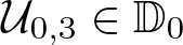 ${\mathcal{U}}_{0,3}\in {\mathbb{D}}_0$,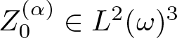 $Z^{(\alpha)}_0\in L^2({\omega})^3$,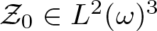 ${\mathcal{Z}}_0\in L^2({\omega})^3$, and $\overline{v}_0^{(\alpha)}\in L^2({\omega}\times (0,1)_{y_\alpha};H^1\big({\mathfrak{I}}^2\big)\big)^3$ satisfying (6.19) such that
 \begin{equation*}
\textbf{J}\big({\mathcal{U}}_{0,3},\widehat v^{(1)}_0, \widehat v^{(2)}_0\big) \leq \liminf_{(\varepsilon,\delta)\to(0,0)}{\textbf{m}_{\varepsilon\delta}\over \varepsilon^2\delta^3}.
\end{equation*}
\begin{equation*}
\textbf{J}\big({\mathcal{U}}_{0,3},\widehat v^{(1)}_0, \widehat v^{(2)}_0\big) \leq \liminf_{(\varepsilon,\delta)\to(0,0)}{\textbf{m}_{\varepsilon\delta}\over \varepsilon^2\delta^3}.
\end{equation*} Moreover,  $\widehat v^{(\alpha)}_0\in L^2\big({\omega};\textbf{L}^2\big((0,1)_{y_\alpha};H^1\big({\mathfrak{I}}^2\big)\big)^3\big)$ is given by
 \begin{equation}
\widehat v_0^{(2)}=\overline{v}_0^{(2)}+y_1 Z_0^{(2)}+y_1y_2 {\mathcal{Z}}_0,\qquad \widehat v^{(1)}=\overline{v}_0^{(1)}+y_2 Z_0^{(1)}+y_1 y_2 {\mathcal{Z}}_0.
\end{equation}
\begin{equation}
\widehat v_0^{(2)}=\overline{v}_0^{(2)}+y_1 Z_0^{(2)}+y_1y_2 {\mathcal{Z}}_0,\qquad \widehat v^{(1)}=\overline{v}_0^{(1)}+y_2 Z_0^{(1)}+y_1 y_2 {\mathcal{Z}}_0.
\end{equation}Proof. Without loss of generality, we can assume that the sequence 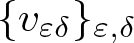 $\{v_{\varepsilon\delta}\}_{\varepsilon,\delta}$ satisfies $\textbf{J}_{\varepsilon\delta}(v_{\varepsilon\delta})\leq \textbf{J}_{\varepsilon\delta}(I_d)=0$. Then, due to (4.66)–(4.67), we have
 \begin{align*}c_0\textbf{D}(v_{\varepsilon\delta})^2&-\int_{\Omega_{\delta}}f_{\varepsilon\delta}\cdot(v_{\varepsilon\delta}-I_d)\,dx\leq c_0\|(\nabla v_{\varepsilon\delta})^T(\nabla v_{\varepsilon\delta})-\textbf{I}_3\|^2_{L^2(\Omega^S_{\varepsilon\delta})}\\
&-\int_{\Omega_{\delta}}f_{\varepsilon\delta}\cdot(v_{\varepsilon\delta}-I_d)\,dx\leq \textbf{J}_{\varepsilon\delta}(v_{\varepsilon\delta})\leq 0.\end{align*}
\begin{align*}c_0\textbf{D}(v_{\varepsilon\delta})^2&-\int_{\Omega_{\delta}}f_{\varepsilon\delta}\cdot(v_{\varepsilon\delta}-I_d)\,dx\leq c_0\|(\nabla v_{\varepsilon\delta})^T(\nabla v_{\varepsilon\delta})-\textbf{I}_3\|^2_{L^2(\Omega^S_{\varepsilon\delta})}\\
&-\int_{\Omega_{\delta}}f_{\varepsilon\delta}\cdot(v_{\varepsilon\delta}-I_d)\,dx\leq \textbf{J}_{\varepsilon\delta}(v_{\varepsilon\delta})\leq 0.\end{align*}Thus, from Lemma 4.14, we obtain
 \begin{equation}
\textbf{D}(v_{\varepsilon\delta})+\|(\nabla v_{\varepsilon\delta})^T\nabla v_{\varepsilon\delta}-\textbf{I}_3\|_{L^2(\Omega^S_{\varepsilon\delta})}\leq C\varepsilon\delta^{3/2}.
\end{equation}
\begin{equation}
\textbf{D}(v_{\varepsilon\delta})+\|(\nabla v_{\varepsilon\delta})^T\nabla v_{\varepsilon\delta}-\textbf{I}_3\|_{L^2(\Omega^S_{\varepsilon\delta})}\leq C\varepsilon\delta^{3/2}.
\end{equation} The constant is independent of  $\varepsilon$ and $\delta$.
Below, we apply the decomposition given in (4.35) for the deformation  $v_{\varepsilon\delta}$. As in Section 6, we use the estimate (6.2) and the convergences stated in Lemma 6.1, Theorem 6.4, and Proposition 6.2, at least for a subsequence (still denoted by the same symbol).
Observe that, using the estimate (7.7) $_2$ and the convergence (6.29), and following the arguments of Theorem 6.4, there exist functions ${\mathcal{U}}_{0,3}^{(3-\alpha)}\in H_{(0,l)}^{2}\big((0,L)_{x_\alpha}\big)$ with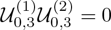 ${\mathcal{U}}_{0,3}^{(1)}{\mathcal{U}}_{0,3}^{(2)}=0$ a.e. in $(0,L)$,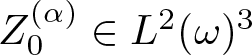 $Z_0^{(\alpha)}\in L^2({\omega})^3$,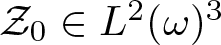 ${\mathcal{Z}}_0\in L^2({\omega})^3$, and $\overline{v}^{(\alpha)}_0\in L^2({\omega}\times (0,1){y_\alpha};H^1({\mathfrak{I}}^2))^3$ satisfying (6.19), such that
 \begin{equation}
\begin{aligned}
{1\over 2\varepsilon\sqrt{{\varepsilon\delta}}}\Pi^{(1)}_{\varepsilon\delta}\big((\nabla v_{\varepsilon\delta})^T(\nabla v_{\varepsilon\delta})-\textbf{I}_3\big) &\rightharpoonup E^{(1)}({\mathcal{U}}_{0,3}^{(1)},\widehat v^{(1)}_0)\quad&&\text{weakly in }\; L^2({\omega}\times {\mathcal{Y}}_1)^{3\times 3},\\
{1\over 2\varepsilon\sqrt{{\varepsilon\delta}}}\Pi^{(2)}_{\varepsilon\delta}\big((\nabla v_{\varepsilon\delta})^T(\nabla v_{\varepsilon\delta})-\textbf{I}_3\big) &\rightharpoonup E^{(2)}({\mathcal{U}}_{0,3}^{(2)},\widehat v^{(2)}_0)\quad&&\text{weakly in }\; L^2({\omega}\times {\mathcal{Y}}_2)^{3\times 3},
\end{aligned}
\end{equation}
\begin{equation}
\begin{aligned}
{1\over 2\varepsilon\sqrt{{\varepsilon\delta}}}\Pi^{(1)}_{\varepsilon\delta}\big((\nabla v_{\varepsilon\delta})^T(\nabla v_{\varepsilon\delta})-\textbf{I}_3\big) &\rightharpoonup E^{(1)}({\mathcal{U}}_{0,3}^{(1)},\widehat v^{(1)}_0)\quad&&\text{weakly in }\; L^2({\omega}\times {\mathcal{Y}}_1)^{3\times 3},\\
{1\over 2\varepsilon\sqrt{{\varepsilon\delta}}}\Pi^{(2)}_{\varepsilon\delta}\big((\nabla v_{\varepsilon\delta})^T(\nabla v_{\varepsilon\delta})-\textbf{I}_3\big) &\rightharpoonup E^{(2)}({\mathcal{U}}_{0,3}^{(2)},\widehat v^{(2)}_0)\quad&&\text{weakly in }\; L^2({\omega}\times {\mathcal{Y}}_2)^{3\times 3},
\end{aligned}
\end{equation}where  $\widehat v^{(\alpha)}_0$ is given by (7.6), and ${\mathcal{U}}_{0,3}^{(2)} + {\mathcal{U}}^{(1)}_{0,3} = {\mathcal{U}}_{0,3} \in {\mathbb{D}}_0$.
Then, using the assumption on the forces (4.60), together with the expression (4.63), and applying the convergences (6.5) $_{1,2}$ and the estimate (6.4) $_1$, we obtain
 \begin{equation}
\begin{aligned}
&\lim_{(\varepsilon,\delta)\to(0,0)}{1\over \varepsilon^2\delta^3}\int_{\Omega_\delta}f_{\varepsilon\delta}\cdot (v_{\varepsilon\delta}-I_d)\,dx\\
&\hskip 5mm= \lim_{(\varepsilon,\delta)\to(0,0)}\big({1\over \varepsilon^2\delta^2}\int_{{\omega}_\delta}\hskip -3mmf_{\varepsilon\delta}\cdot({\mathcal{V}}_{\varepsilon\delta}-I_d)\,dx'+{1\over \varepsilon^3\delta}\int_{{\omega}\times {\mathcal{Y}}_\alpha}\hskip -3mm\Pi_{\varepsilon\delta}^{(\alpha)}\big(f_{\varepsilon\delta}\cdot \overline{v}_{\varepsilon\delta}\big)\,dx'dy\big)\\
&\hskip 5mm=\int_{{\omega}} f\cdot{\mathcal{U}}_0\,dx'.
\end{aligned}
\end{equation}
\begin{equation}
\begin{aligned}
&\lim_{(\varepsilon,\delta)\to(0,0)}{1\over \varepsilon^2\delta^3}\int_{\Omega_\delta}f_{\varepsilon\delta}\cdot (v_{\varepsilon\delta}-I_d)\,dx\\
&\hskip 5mm= \lim_{(\varepsilon,\delta)\to(0,0)}\big({1\over \varepsilon^2\delta^2}\int_{{\omega}_\delta}\hskip -3mmf_{\varepsilon\delta}\cdot({\mathcal{V}}_{\varepsilon\delta}-I_d)\,dx'+{1\over \varepsilon^3\delta}\int_{{\omega}\times {\mathcal{Y}}_\alpha}\hskip -3mm\Pi_{\varepsilon\delta}^{(\alpha)}\big(f_{\varepsilon\delta}\cdot \overline{v}_{\varepsilon\delta}\big)\,dx'dy\big)\\
&\hskip 5mm=\int_{{\omega}} f\cdot{\mathcal{U}}_0\,dx'.
\end{aligned}
\end{equation}We claim that
 \begin{equation}
\begin{aligned}
\textbf{1}_{({\omega}\setminus{\omega}_{\varepsilon\delta}^J)\times {\mathcal{Y}}_1}\big({1\over \varepsilon\sqrt{{\varepsilon\delta}}}\Pi_{\varepsilon\delta}^{(1)}\big(\textbf{E}(\nabla v_{\varepsilon\delta})\big)\big)\rightharpoonup E^{(1)}({\mathcal{U}}_{0,3}^{(1)},\widehat v_0^{(1)})\quad \text{weakly in}\ L^2({\omega}\times {\mathcal{Y}}_1)^{3\times 3},\\
\textbf{1}_{({\omega}\setminus{\omega}_{\varepsilon\delta}^J)\times {\mathcal{Y}}_2}\big({1\over \varepsilon\sqrt{{\varepsilon\delta}}}\Pi_{\varepsilon\delta}^{(2)}\big(\textbf{E}(\nabla v_{\varepsilon\delta})\big)\big)\rightharpoonup E^{(2)}({\mathcal{U}}_{0,3}^{(2)},\widehat v^{(2)}_0)\quad \text{weakly in}\ L^2({\omega}\times {\mathcal{Y}}_2)^{3\times 3},
\end{aligned}
\end{equation}
\begin{equation}
\begin{aligned}
\textbf{1}_{({\omega}\setminus{\omega}_{\varepsilon\delta}^J)\times {\mathcal{Y}}_1}\big({1\over \varepsilon\sqrt{{\varepsilon\delta}}}\Pi_{\varepsilon\delta}^{(1)}\big(\textbf{E}(\nabla v_{\varepsilon\delta})\big)\big)\rightharpoonup E^{(1)}({\mathcal{U}}_{0,3}^{(1)},\widehat v_0^{(1)})\quad \text{weakly in}\ L^2({\omega}\times {\mathcal{Y}}_1)^{3\times 3},\\
\textbf{1}_{({\omega}\setminus{\omega}_{\varepsilon\delta}^J)\times {\mathcal{Y}}_2}\big({1\over \varepsilon\sqrt{{\varepsilon\delta}}}\Pi_{\varepsilon\delta}^{(2)}\big(\textbf{E}(\nabla v_{\varepsilon\delta})\big)\big)\rightharpoonup E^{(2)}({\mathcal{U}}_{0,3}^{(2)},\widehat v^{(2)}_0)\quad \text{weakly in}\ L^2({\omega}\times {\mathcal{Y}}_2)^{3\times 3},
\end{aligned}
\end{equation}where 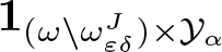 $\textbf{1}_{({\omega}\setminus{\omega}_{\varepsilon\delta}^J)\times {\mathcal{Y}}_\alpha}$ is the characteristic function for ${({\omega}\setminus{\omega}_{\varepsilon\delta}^J)\times {\mathcal{Y}}_\alpha}$ where we put
 \begin{equation}
\Omega^J_{\varepsilon\delta}=\Omega_{\varepsilon\delta}^{(1)}\cap\Omega_{\varepsilon\delta}^{(2)}\cap \Omega_\delta\quad \hbox{and}\quad {\omega}^J_{\varepsilon\delta}=\Omega^J_{\varepsilon\delta}\cap {\omega}_\delta.
\end{equation}
\begin{equation}
\Omega^J_{\varepsilon\delta}=\Omega_{\varepsilon\delta}^{(1)}\cap\Omega_{\varepsilon\delta}^{(2)}\cap \Omega_\delta\quad \hbox{and}\quad {\omega}^J_{\varepsilon\delta}=\Omega^J_{\varepsilon\delta}\cap {\omega}_\delta.
\end{equation} We have  $\displaystyle \textbf{1}_{({\omega}\setminus{\omega}_{\varepsilon\delta}^J)\times {\mathcal{Y}}_\alpha}\in L^\infty({\omega}\times {\mathcal{Y}}_\alpha)$. Then, since $|{\omega}\times {\mathcal{Y}}_\alpha|=L^2$ and $\displaystyle |{\omega}_{\varepsilon\delta}^J\times {\mathcal{Y}}_\alpha|=4\delta^2|{\mathcal{K}}_\varepsilon|^2=\textbf{O}\Big({\delta^2\over \varepsilon^2}\Big)$, so $|{\omega}^J_{\varepsilon\delta}\times {\mathcal{Y}}_\alpha|\to0$. Hence
 \begin{equation}
\textbf{1}_{({\omega}\setminus{\omega}_{\varepsilon\delta}^J)\times {\mathcal{Y}}_\alpha}(x',y)\to \textbf{1}_{{\omega}\times {\mathcal{Y}}_\alpha}(x',y) \quad \hbox{for a.e. } (x',y)\in {\omega}\times {\mathcal{Y}}_\alpha.
\end{equation}
\begin{equation}
\textbf{1}_{({\omega}\setminus{\omega}_{\varepsilon\delta}^J)\times {\mathcal{Y}}_\alpha}(x',y)\to \textbf{1}_{{\omega}\times {\mathcal{Y}}_\alpha}(x',y) \quad \hbox{for a.e. } (x',y)\in {\omega}\times {\mathcal{Y}}_\alpha.
\end{equation} Using the estimate (7.7) $_2$ and properties of re-scaling operator (5.2), we have
 \begin{align*}
&\left\|\Pi_{\varepsilon\delta}^{(\alpha)}\big(\textbf{E}(\nabla v_{\varepsilon\delta})\big)\right\|_{L^2({\omega}\times {\mathcal{Y}}_\alpha)}\leq C\varepsilon\sqrt{{\varepsilon\delta}}\\
&\quad \implies
\Big\|\textbf{1}_{({\omega}\setminus{\omega}_{\varepsilon\delta}^J)\times {\mathcal{Y}}_\alpha}{1\over \varepsilon\sqrt{{\varepsilon\delta}}}\Pi_{\varepsilon\delta}^{(\alpha)}\big(\textbf{E}(\nabla v_{\varepsilon\delta})\big)\Big\|_{L^2({\omega}\times {\mathcal{Y}}_\alpha)}\leq C.\end{align*}
\begin{align*}
&\left\|\Pi_{\varepsilon\delta}^{(\alpha)}\big(\textbf{E}(\nabla v_{\varepsilon\delta})\big)\right\|_{L^2({\omega}\times {\mathcal{Y}}_\alpha)}\leq C\varepsilon\sqrt{{\varepsilon\delta}}\\
&\quad \implies
\Big\|\textbf{1}_{({\omega}\setminus{\omega}_{\varepsilon\delta}^J)\times {\mathcal{Y}}_\alpha}{1\over \varepsilon\sqrt{{\varepsilon\delta}}}\Pi_{\varepsilon\delta}^{(\alpha)}\big(\textbf{E}(\nabla v_{\varepsilon\delta})\big)\Big\|_{L^2({\omega}\times {\mathcal{Y}}_\alpha)}\leq C.\end{align*}Together with (7.12) and the weak convergence (7.8) gives (7.10).
Using the unfolding operator, we transform  $\textbf{W}_{\varepsilon\delta}$ (see (3.3) for the definition) to get,
 \begin{equation*}
\begin{aligned}
&{1\over \varepsilon^2\delta^3}\int_{\Omega^S_{\varepsilon\delta}}\textbf{W}_{\varepsilon\delta}(x,\nabla v_{\varepsilon\delta})\,dx
\geq \sum_{\alpha=1}^2{1\over \varepsilon^2\delta^3}\int_{\Omega^{(\alpha)}_{\varepsilon\delta}\setminus \Omega^J_{\varepsilon\delta}}\textbf{W}_{\varepsilon\delta}(x,\nabla v_{\varepsilon\delta})\,dx\\
&\geq \sum_{\alpha=1}^2\int_{{\omega}\times {\mathcal{Y}}_\alpha} \left\langle \textbf{1}_{({\omega}\setminus{\omega}_{\varepsilon\delta}^J)\times {\mathcal{Y}}_\alpha}\big({1\over \varepsilon\sqrt{{\varepsilon\delta}}}\Pi_{\varepsilon\delta}^{(\alpha)}\big(\textbf{E}(\nabla v_{\varepsilon\delta})\big)\big)\Pi^{(\alpha)}_{\varepsilon\delta}({\mathbb{A}}_{{\varepsilon\delta}}), \right.\\
&\left.\quad {1\over \varepsilon\sqrt{{\varepsilon\delta}}}\Pi_{\varepsilon\delta}^{(\alpha)}\big(\textbf{E}(\nabla v_{\varepsilon\delta})\big)\right\rangle\,dx'dy.
\end{aligned}
\end{equation*}
\begin{equation*}
\begin{aligned}
&{1\over \varepsilon^2\delta^3}\int_{\Omega^S_{\varepsilon\delta}}\textbf{W}_{\varepsilon\delta}(x,\nabla v_{\varepsilon\delta})\,dx
\geq \sum_{\alpha=1}^2{1\over \varepsilon^2\delta^3}\int_{\Omega^{(\alpha)}_{\varepsilon\delta}\setminus \Omega^J_{\varepsilon\delta}}\textbf{W}_{\varepsilon\delta}(x,\nabla v_{\varepsilon\delta})\,dx\\
&\geq \sum_{\alpha=1}^2\int_{{\omega}\times {\mathcal{Y}}_\alpha} \left\langle \textbf{1}_{({\omega}\setminus{\omega}_{\varepsilon\delta}^J)\times {\mathcal{Y}}_\alpha}\big({1\over \varepsilon\sqrt{{\varepsilon\delta}}}\Pi_{\varepsilon\delta}^{(\alpha)}\big(\textbf{E}(\nabla v_{\varepsilon\delta})\big)\big)\Pi^{(\alpha)}_{\varepsilon\delta}({\mathbb{A}}_{{\varepsilon\delta}}), \right.\\
&\left.\quad {1\over \varepsilon\sqrt{{\varepsilon\delta}}}\Pi_{\varepsilon\delta}^{(\alpha)}\big(\textbf{E}(\nabla v_{\varepsilon\delta})\big)\right\rangle\,dx'dy.
\end{aligned}
\end{equation*} So, the above inequality along with convergences (7.9) and (7.10) together with the weak lower semi-continuity of the function  $\textbf{J}_{\varepsilon\delta}$ give
 \begin{equation*}\liminf_{(\varepsilon,\delta)\to(0,0)}{\textbf{J}_{\varepsilon\delta}(v_{\varepsilon\delta})\over \varepsilon^2\delta^3}\geq\textbf{J}\big({\mathcal{U}}_{0,3},\widehat v_0^{(1)},\widehat v_0^{(2)}\big).\end{equation*}
Finally, using the equation (7.5), we obtain
 \begin{equation*}\liminf_{(\varepsilon,\delta)\to(0,0)}{\textbf{m}_{\varepsilon\delta}\over \varepsilon^2\delta^3}=\liminf_{(\varepsilon,\delta)\to(0,0)} {\textbf{J}_{\varepsilon\delta}(v_{\varepsilon\delta})\over \varepsilon^2\delta^3}\geq\textbf{J}\big({\mathcal{U}}_{0,3},\widehat v_0^{(1)},\widehat v_0^{(2)}\big).\end{equation*}
This completes the proof.
7.2. Existence of a minimizer for the limit unfolded energy
In this subsection, we prove the existence of a minimizer of the limit unfolded energy. For that we give a preliminary estimate and a coercivity result.
Denote
 \begin{equation*}
\begin{aligned}
{\mathfrak{W}}({\mathcal{Y}}_1)=& \Big\{\widehat {v}\in L^2\big((0,1)_{y_1};H^1\big({\mathfrak{I}}^2\big)\big)^3 \;|\; \widehat v=\overline{v}+ \textbf{a} y_2 +\textbf{b} y_1y_2 +{\mathcal{G}} y_2y_3,\\
&(\textbf{a},\textbf{b},{\mathcal{G}})\in {\mathbb{R}}^{3\times 3} \hskip 5mm\hbox{and }\ \ \overline{v}\in L^2\big((0,1)_{y_1};H^1\big({\mathfrak{I}}^2\big)\big)^3\\
&\quad \text{with}\quad\overline{v}=0\ \ \text{a.e. on } (0,1)\times \{\pm{1\over 2}\}\times {\mathfrak{I}}\Big\}.
\end{aligned}
\end{equation*}
\begin{equation*}
\begin{aligned}
{\mathfrak{W}}({\mathcal{Y}}_1)=& \Big\{\widehat {v}\in L^2\big((0,1)_{y_1};H^1\big({\mathfrak{I}}^2\big)\big)^3 \;|\; \widehat v=\overline{v}+ \textbf{a} y_2 +\textbf{b} y_1y_2 +{\mathcal{G}} y_2y_3,\\
&(\textbf{a},\textbf{b},{\mathcal{G}})\in {\mathbb{R}}^{3\times 3} \hskip 5mm\hbox{and }\ \ \overline{v}\in L^2\big((0,1)_{y_1};H^1\big({\mathfrak{I}}^2\big)\big)^3\\
&\quad \text{with}\quad\overline{v}=0\ \ \text{a.e. on } (0,1)\times \{\pm{1\over 2}\}\times {\mathfrak{I}}\Big\}.
\end{aligned}
\end{equation*}We have
Lemma 7.2. There exists a constant  $C$ strictly positive such that for all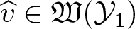 $ \widehat v\in {\mathfrak{W}}({\mathcal{Y}}_1)$
 \begin{equation}\begin{aligned}
\|\overline{v}\|_{L^2({\mathcal{Y}}_1)}+\|\partial_{y_2}\overline{v}\|_{L^2({\mathcal{Y}}_1)}+\|\partial_{y_3}\overline{v}\|_{L^2({\mathcal{Y}}_1)}+|\textbf{a}|+|\textbf{b}|+|{\mathcal{G}}|\\
\leq C\Big(\|\partial_{y_2}\widehat v_1\|_{L^2({\mathcal{Y}}_1)}+\|\partial_{y_3}\widehat v_1\|_{L^2({\mathcal{Y}}_1)}+\|e_{22,y}(\widehat v)\|_{L^2({\mathcal{Y}}_1)}\\
+\|e_{23,y}(\widehat v)\|_{L^2({\mathcal{Y}}_1)}+\|e_{33,y}(\widehat v)\|_{L^2({\mathcal{Y}}_1)}\big).
\end{aligned}
\end{equation}
\begin{equation}\begin{aligned}
\|\overline{v}\|_{L^2({\mathcal{Y}}_1)}+\|\partial_{y_2}\overline{v}\|_{L^2({\mathcal{Y}}_1)}+\|\partial_{y_3}\overline{v}\|_{L^2({\mathcal{Y}}_1)}+|\textbf{a}|+|\textbf{b}|+|{\mathcal{G}}|\\
\leq C\Big(\|\partial_{y_2}\widehat v_1\|_{L^2({\mathcal{Y}}_1)}+\|\partial_{y_3}\widehat v_1\|_{L^2({\mathcal{Y}}_1)}+\|e_{22,y}(\widehat v)\|_{L^2({\mathcal{Y}}_1)}\\
+\|e_{23,y}(\widehat v)\|_{L^2({\mathcal{Y}}_1)}+\|e_{33,y}(\widehat v)\|_{L^2({\mathcal{Y}}_1)}\big).
\end{aligned}
\end{equation}Proof. See Appendix A.
We also have the following coercivity result:
Lemma 7.3. There exists a strictly positive constant  $C$ such that
 \begin{equation}
\begin{aligned}
&\|d^2_{22}{\mathcal{U}}_3^{(1)}\|^2_{L^2({\omega})}+\|Z^{(1)}\|^2_{L^2({\omega})}+\|{\mathcal{Z}}\|^2_{L^2({\omega})}+\|\overline{v}^{(1)}\|^2_{L^2({\omega}\times (0,1)_{y_1};H^1({\mathfrak{I}}^2))}\\
&\hskip 75mm \leq C\|E^{(1)}({\mathcal{U}}_3^{(1)},\widehat v^{(1)})\|^2_{L^2({\omega}\times {\mathcal{Y}}_1)},\\
&\|d^2_{11}{\mathcal{U}}_3^{(2)}\|^2_{L^2({\omega})}+\|Z^{(2)}\|^2_{L^2({\omega})}+\|{\mathcal{Z}}\|^2_{L^2({\omega})}+\|\overline{v}^{(2)}\|^2_{L^2({\omega}\times (0,1)_{y_2};H^1({\mathfrak{I}}^2))}\\
&\hskip 75mm \leq C\|E^{(2)}({\mathcal{U}}_3^{(2)},\widehat v^{(2)})\|^2_{L^2({\omega}\times {\mathcal{Y}}_2)},
\end{aligned}
\end{equation}
\begin{equation}
\begin{aligned}
&\|d^2_{22}{\mathcal{U}}_3^{(1)}\|^2_{L^2({\omega})}+\|Z^{(1)}\|^2_{L^2({\omega})}+\|{\mathcal{Z}}\|^2_{L^2({\omega})}+\|\overline{v}^{(1)}\|^2_{L^2({\omega}\times (0,1)_{y_1};H^1({\mathfrak{I}}^2))}\\
&\hskip 75mm \leq C\|E^{(1)}({\mathcal{U}}_3^{(1)},\widehat v^{(1)})\|^2_{L^2({\omega}\times {\mathcal{Y}}_1)},\\
&\|d^2_{11}{\mathcal{U}}_3^{(2)}\|^2_{L^2({\omega})}+\|Z^{(2)}\|^2_{L^2({\omega})}+\|{\mathcal{Z}}\|^2_{L^2({\omega})}+\|\overline{v}^{(2)}\|^2_{L^2({\omega}\times (0,1)_{y_2};H^1({\mathfrak{I}}^2))}\\
&\hskip 75mm \leq C\|E^{(2)}({\mathcal{U}}_3^{(2)},\widehat v^{(2)})\|^2_{L^2({\omega}\times {\mathcal{Y}}_2)},
\end{aligned}
\end{equation}for all  ${\mathcal{U}}_3^{(3-\alpha)}\in H_{(0,l)}^{2}\big((0,L)_{x_\alpha}\big)$ and $\widehat v^{(\alpha)}\in L^2\big({\omega};\textbf{L}^2\big((0,1)_{y_\alpha};H^1\big({\mathfrak{I}}^2\big)\big)^3\big)$.
Proof. See Appendix A.
The following is the main result of this subsection.
Proposition 7.4. There exist a  $({\mathcal{W}}_3, \widehat {w}^{(1)}, \widehat {w}^{(2)})\in {\mathbb{D}}$ such that
 \begin{equation*}
\textbf{J}({\mathcal{W}}_3,\widehat w^{(1)},\widehat w^{(2)})= \textbf{m}
= \inf_{({\mathcal{U}}_{3},\widehat v^{(1)},\widehat v^{(2)})\in {\mathbb{D}}}\textbf{J}({\mathcal{U}}_3,\widehat v^{(1)},\widehat v^{(2)}),
\end{equation*}
\begin{equation*}
\textbf{J}({\mathcal{W}}_3,\widehat w^{(1)},\widehat w^{(2)})= \textbf{m}
= \inf_{({\mathcal{U}}_{3},\widehat v^{(1)},\widehat v^{(2)})\in {\mathbb{D}}}\textbf{J}({\mathcal{U}}_3,\widehat v^{(1)},\widehat v^{(2)}),
\end{equation*}where
 \begin{equation*}
\begin{aligned}
&{\mathcal{W}}(x')={\mathcal{W}}_{1}(x_1)\textbf{e}_1+{\mathcal{W}}_{2}(x_2)\textbf{e}_2+{\mathcal{W}}_{3}(x')\textbf{e}_3\quad\text{for a.e.}\ x'\in{\omega},\\
&d_\alpha{\mathcal{W}}_{\alpha}=-{1\over 2}\big|d_\alpha{\mathcal{W}}_{3}^{(3-\alpha)}\big|^2,\; {\mathcal{W}}_3={\mathcal{W}}_3^{(2)}+{\mathcal{W}}_3^{(1)}\,\text{and}\quad {\mathcal{W}}_3^{(1)}{\mathcal{W}}_3^{(2)}=0,\,\text{a.e. in}\ (0,L),\\
& {\mathcal{W}}_{\alpha}\in H_{(0,l)}^{1}\big((0,L)_{x_\alpha}\big),\; {\mathcal{W}}_3^{(3-\alpha)}\in H_{(0,l)}^{2}\big((0,L)_{x_\alpha}\big).
\end{aligned}
\end{equation*}
\begin{equation*}
\begin{aligned}
&{\mathcal{W}}(x')={\mathcal{W}}_{1}(x_1)\textbf{e}_1+{\mathcal{W}}_{2}(x_2)\textbf{e}_2+{\mathcal{W}}_{3}(x')\textbf{e}_3\quad\text{for a.e.}\ x'\in{\omega},\\
&d_\alpha{\mathcal{W}}_{\alpha}=-{1\over 2}\big|d_\alpha{\mathcal{W}}_{3}^{(3-\alpha)}\big|^2,\; {\mathcal{W}}_3={\mathcal{W}}_3^{(2)}+{\mathcal{W}}_3^{(1)}\,\text{and}\quad {\mathcal{W}}_3^{(1)}{\mathcal{W}}_3^{(2)}=0,\,\text{a.e. in}\ (0,L),\\
& {\mathcal{W}}_{\alpha}\in H_{(0,l)}^{1}\big((0,L)_{x_\alpha}\big),\; {\mathcal{W}}_3^{(3-\alpha)}\in H_{(0,l)}^{2}\big((0,L)_{x_\alpha}\big).
\end{aligned}
\end{equation*}Proof. Observe that
 \begin{equation*}\textbf{m}\leq \textbf{J}(0,0,0)=0,\quad \text{since}\ (0,0,0)\in {\mathbb{D}},\end{equation*}
which imply  $\textbf{m}\in [-\infty,0]$.
Step 1. We show that  $\textbf{m}\in(-\infty,0]$. Let $({\mathcal{U}}_{3},\widehat v^{(1)},\widehat v^{(2)})\in{\mathbb{D}}$ be such that
 \begin{equation}
\textbf{J}({\mathcal{U}}_3,\widehat v^{(1)},\widehat v^{(2)})\leq \textbf{J}(0,0,0)=0.
\end{equation}
\begin{equation}
\textbf{J}({\mathcal{U}}_3,\widehat v^{(1)},\widehat v^{(2)})\leq \textbf{J}(0,0,0)=0.
\end{equation} Since,  $\widehat v^{(\alpha)}\in L^2\big({\omega}; \textbf{L}^2\big((0,1)_{y_\alpha};H^1\big({\mathfrak{I}}^2\big)\big)^3 \big)$, there exist $\overline{v}^{(\alpha)}$, $Z^{(\alpha)}$, and ${\mathcal{Z}}$ such that $\overline{v}^{(\alpha)}$ satisfies (6.19) and $\widehat v^{(\alpha)}$ is given by (6.30). We have ${\mathcal{U}}_3^{(3-\alpha)}\in H_{(0,l)}^{2}\big((0,L)_{x_\alpha}\big)$ such that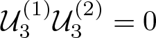 ${\mathcal{U}}_3^{(1)}{\mathcal{U}}_3^{(2)}=0$ a.e. in $(0,L)$. So, using the Coercivity (7.4) of $\textbf{Q}^{(\alpha)}$ and (7.14), there exists $0 \lt C\in{\mathbb{R}}$ such that
 \begin{equation}
\begin{aligned}
\|d^2_{22}{\mathcal{U}}_3^{(1)}\|^2_{L^2({\omega})}+\|Z^{(1)}\|^2_{L^2({\omega})}&+\|{\mathcal{Z}}\|^2_{L^2({\omega})}+\|\widehat v^{(1)}\|^2_{L^2({\omega}\times (0,1)_{y_1};H^1({\mathfrak{I}}^2))}\\
& \leq C\|E^{(1)}({\mathcal{U}}_3^{(1)},\widehat v^{(1)})\|^2_{L^2({\omega}\times {\mathcal{Y}}_1)}\\
&\leq C\int_{{\omega}\times {\mathcal{Y}}_1}\textbf{Q}^{(1)}(y,E^{(1)}({\mathcal{U}}_3^{(1)},\widehat v^{(1)}))\,dydx',\\
\|d^2_{11}{\mathcal{U}}_3^{(2)}\|^2_{L^2({\omega})}+\|Z^{(2)}\|^2_{L^2({\omega})}&+\|{\mathcal{Z}}\|^2_{L^2({\omega})}+\|\widehat v^{(2)}\|^2_{L^2({\omega}\times (0,1)_{y_2};H^1({\mathfrak{I}}^2))}\\
&\leq C\|E^{(2)}({\mathcal{U}}_3^{(2)},\widehat v^{(2)})\|^2_{L^2({\omega}\times {\mathcal{Y}}_2)}\\
&\leq C\int_{{\omega}\times {\mathcal{Y}}_2}\textbf{Q}^{(2)}(y,E^{(2)}({\mathcal{U}}_3^{(2)},\widehat v^{(2)}))\,dydx'.
\end{aligned}
\end{equation}
\begin{equation}
\begin{aligned}
\|d^2_{22}{\mathcal{U}}_3^{(1)}\|^2_{L^2({\omega})}+\|Z^{(1)}\|^2_{L^2({\omega})}&+\|{\mathcal{Z}}\|^2_{L^2({\omega})}+\|\widehat v^{(1)}\|^2_{L^2({\omega}\times (0,1)_{y_1};H^1({\mathfrak{I}}^2))}\\
& \leq C\|E^{(1)}({\mathcal{U}}_3^{(1)},\widehat v^{(1)})\|^2_{L^2({\omega}\times {\mathcal{Y}}_1)}\\
&\leq C\int_{{\omega}\times {\mathcal{Y}}_1}\textbf{Q}^{(1)}(y,E^{(1)}({\mathcal{U}}_3^{(1)},\widehat v^{(1)}))\,dydx',\\
\|d^2_{11}{\mathcal{U}}_3^{(2)}\|^2_{L^2({\omega})}+\|Z^{(2)}\|^2_{L^2({\omega})}&+\|{\mathcal{Z}}\|^2_{L^2({\omega})}+\|\widehat v^{(2)}\|^2_{L^2({\omega}\times (0,1)_{y_2};H^1({\mathfrak{I}}^2))}\\
&\leq C\|E^{(2)}({\mathcal{U}}_3^{(2)},\widehat v^{(2)})\|^2_{L^2({\omega}\times {\mathcal{Y}}_2)}\\
&\leq C\int_{{\omega}\times {\mathcal{Y}}_2}\textbf{Q}^{(2)}(y,E^{(2)}({\mathcal{U}}_3^{(2)},\widehat v^{(2)}))\,dydx'.
\end{aligned}
\end{equation} The above inequalities along with the boundary condition satisfied by  ${\mathcal{U}}_3^{(\alpha)}$, and using Poincaré inequality we obtain
 \begin{align}
\|{\mathcal{U}}_3^{(2)}\|^2_{H^2(0,L)}+\|{\mathcal{U}}_3^{(1)}\|^2_{H^2(0,L)}&\leq C\big(\|d^2_{11}{\mathcal{U}}_3^{(2)}\|^2_{L^2(0,L)}+\|d^2_{22}{\mathcal{U}}_3^{(1)}\|^2_{L^2(0,L)}) \nonumber\\
&\leq C\textbf{W}({\mathcal{U}}_3,\widehat v^{(1)},\widehat v^{(2)}).
\end{align}
\begin{align}
\|{\mathcal{U}}_3^{(2)}\|^2_{H^2(0,L)}+\|{\mathcal{U}}_3^{(1)}\|^2_{H^2(0,L)}&\leq C\big(\|d^2_{11}{\mathcal{U}}_3^{(2)}\|^2_{L^2(0,L)}+\|d^2_{22}{\mathcal{U}}_3^{(1)}\|^2_{L^2(0,L)}) \nonumber\\
&\leq C\textbf{W}({\mathcal{U}}_3,\widehat v^{(1)},\widehat v^{(2)}).
\end{align} Since,  ${\mathcal{U}}_{\alpha}\in H_{(0,l)}^{1}\big((0,L)_{x_\alpha}\big)$ and $d_\alpha{\mathcal{U}}_{\alpha}=-{1\over 2}|d_\alpha{\mathcal{U}}_3^{(3-\alpha)}|^2$ a.e. in $(0,L)$, we get
 \begin{equation*}\|d_\alpha{\mathcal{U}}_{\alpha}\|^2_{L^2(0,L)}\leq C\|d_\alpha{\mathcal{U}}_3^{(3-\alpha)}\|^4_{L^4(0,L)}.\end{equation*}
 Using Poincaré inequality, (7.17) and the fact that 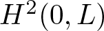 $H^2(0,L)$ is continuously embedded in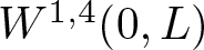 $W^{1,4}(0,L)$, we get
 \begin{equation}
\sum_{{\alpha}=1}^2\|{\mathcal{U}}_{\alpha}\|^2_{L^2(0,L)}\leq C\sum_{{\alpha}=1}^2\|{\mathcal{U}}_3^{(3-\alpha)}\|^4_{H^2(0,L)}\leq C\left[\textbf{W}({\mathcal{U}}_3,\widehat v^{(1)},\widehat v^{(2)})\right]^2.
\end{equation}
\begin{equation}
\sum_{{\alpha}=1}^2\|{\mathcal{U}}_{\alpha}\|^2_{L^2(0,L)}\leq C\sum_{{\alpha}=1}^2\|{\mathcal{U}}_3^{(3-\alpha)}\|^4_{H^2(0,L)}\leq C\left[\textbf{W}({\mathcal{U}}_3,\widehat v^{(1)},\widehat v^{(2)})\right]^2.
\end{equation}From (7.15) along with (7.17)–(7.18), we get
 \begin{equation*}
\begin{aligned}
\textbf{W}\big({\mathcal{U}}_{3},\widehat v^{(1)},\widehat v^{(2)}\big) &\leq \left|\int_{\omega} f\cdot {\mathcal{U}}\,dx'\right|\\
& \leq L \sum_{\alpha=1}^2\big(\|f_\alpha\|_{L^2({\omega})}\|{\mathcal{U}}_\alpha\|_{L^2(0,L)}+\|f_3\|_{L^2({\omega})}\|{\mathcal{U}}_3^{(\alpha)}\|_{L^2(0,L)}\big)\\
&\leq C\left(\sum_{{\alpha}=1}^2\|f_{\alpha}\|_{L^2({\omega})}\right)\left[\textbf{W}({\mathcal{U}}_3,\widehat v^{(1)},\widehat v^{(2)})\right]\\
&\quad +C\|f_3\|_{L^2({\omega})}\left[\sqrt{\textbf{W}({\mathcal{U}}_3,\widehat v^{(1)},\widehat v^{(2)})}\right].
\end{aligned}
\end{equation*}
\begin{equation*}
\begin{aligned}
\textbf{W}\big({\mathcal{U}}_{3},\widehat v^{(1)},\widehat v^{(2)}\big) &\leq \left|\int_{\omega} f\cdot {\mathcal{U}}\,dx'\right|\\
& \leq L \sum_{\alpha=1}^2\big(\|f_\alpha\|_{L^2({\omega})}\|{\mathcal{U}}_\alpha\|_{L^2(0,L)}+\|f_3\|_{L^2({\omega})}\|{\mathcal{U}}_3^{(\alpha)}\|_{L^2(0,L)}\big)\\
&\leq C\left(\sum_{{\alpha}=1}^2\|f_{\alpha}\|_{L^2({\omega})}\right)\left[\textbf{W}({\mathcal{U}}_3,\widehat v^{(1)},\widehat v^{(2)})\right]\\
&\quad +C\|f_3\|_{L^2({\omega})}\left[\sqrt{\textbf{W}({\mathcal{U}}_3,\widehat v^{(1)},\widehat v^{(2)})}\right].
\end{aligned}
\end{equation*} So, from the above inequality along with the assumption of forces (4.61) ( $C\|f_{\alpha}\|_{L^2({\omega})}\leq {1\over 2}$), we get
 \begin{equation*} \textbf{W}\big({\mathcal{U}}_{3},\widehat v^{(1)},\widehat v^{(2)}\big) \leq C\quad\text{and}\quad \left|\int_{\omega} f\cdot {\mathcal{U}}\,dx'\right|\leq C. \end{equation*}
 Finally, if  $({\mathcal{U}}_{3},\widehat v^{(1)},\widehat v^{(2)})\in{\mathbb{D}}$ is such that it satisfies (7.15), then using the above inequality along with (7.16)–(7.18) we obtain for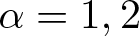 $\alpha=1,2$
 \begin{equation}
\|{\mathcal{U}}_\alpha\|^2_{L^2(0,L)}+\|{\mathcal{U}}_3^{(\alpha)}\|^2_{H^2(0,L)}+\|Z^{(\alpha)}\|^2_{L^2({\omega})}+\|{\mathcal{Z}}\|^2_{L^2({\omega})}+\|\overline{v}^{(\alpha)}\|^2_{L^2({\omega}\times (0,1)_{y_\alpha};H^1({\mathfrak{I}}^2))}\leq C,
\end{equation}
\begin{equation}
\|{\mathcal{U}}_\alpha\|^2_{L^2(0,L)}+\|{\mathcal{U}}_3^{(\alpha)}\|^2_{H^2(0,L)}+\|Z^{(\alpha)}\|^2_{L^2({\omega})}+\|{\mathcal{Z}}\|^2_{L^2({\omega})}+\|\overline{v}^{(\alpha)}\|^2_{L^2({\omega}\times (0,1)_{y_\alpha};H^1({\mathfrak{I}}^2))}\leq C,
\end{equation}and
 \begin{equation*}-C\leq -\int_{\omega} f\cdot {\mathcal{U}},\,dx'\leq \textbf{W}({\mathcal{U}}_3,\widehat v^{(1)},\widehat v^{(2)})-\int_{\omega} f\cdot{\mathcal{U}}\,dx'\leq 0,\end{equation*}
which implies  $\textbf{J}({\mathcal{U}}_3,\widehat v^{(1)},\widehat v^{(2)})\in [-C,0]$. As a consequence, we obtain $\textbf{m}\in(-\infty,0]$.
Step 2: We prove the main statement of the theorem.
Since  $\textbf{m}\in (-\infty,0]$, there exists a minimizing sequence $\{({\mathcal{U}}_{n,3},\widehat v^{(1)}_{n},\widehat v^{(2)}_n)\}_n\subset {\mathbb{D}}$ satisfying (7.15) and
 \begin{equation*}
\textbf{m}=\inf_{({\mathcal{U}}_{3},\widehat v^{(1)},\widehat v^{(2)})\in{\mathbb{D}}}\textbf{J}({\mathcal{U}}_3,\widehat v^{(1)},\widehat v^{(2)})=\liminf_{n\to+\infty}\textbf{J}({\mathcal{U}}_{n,3},\widehat v^{(1)}_n,\widehat v^{(2)}_n),
\end{equation*}
\begin{equation*}
\textbf{m}=\inf_{({\mathcal{U}}_{3},\widehat v^{(1)},\widehat v^{(2)})\in{\mathbb{D}}}\textbf{J}({\mathcal{U}}_3,\widehat v^{(1)},\widehat v^{(2)})=\liminf_{n\to+\infty}\textbf{J}({\mathcal{U}}_{n,3},\widehat v^{(1)}_n,\widehat v^{(2)}_n),
\end{equation*}where
 \begin{align*}
&{\mathcal{U}}_n(x')={\mathcal{U}}_{n,1}(x_1)\textbf{e}_1+{\mathcal{U}}_{n,2}(x_2)\textbf{e}_2+({\mathcal{U}}_{n,3}^{(2)}(x_1)+{\mathcal{U}}_{n,3}^{(1)}(x_2))\textbf{e}_3,\\
& {\mathcal{U}}_{n,3}^{(1)} {\mathcal{U}}_{n,3}^{(2)}=0,\quad\text{a.e. in}\ (0,L),\end{align*}
\begin{align*}
&{\mathcal{U}}_n(x')={\mathcal{U}}_{n,1}(x_1)\textbf{e}_1+{\mathcal{U}}_{n,2}(x_2)\textbf{e}_2+({\mathcal{U}}_{n,3}^{(2)}(x_1)+{\mathcal{U}}_{n,3}^{(1)}(x_2))\textbf{e}_3,\\
& {\mathcal{U}}_{n,3}^{(1)} {\mathcal{U}}_{n,3}^{(2)}=0,\quad\text{a.e. in}\ (0,L),\end{align*}with  ${\mathcal{U}}_{n,\alpha}\in H_{(0,l)}^{1}\big((0,L)_{x_\alpha}\big)$ given by
 \begin{equation*}d_\alpha{\mathcal{U}}_{n,\alpha}=-{1\over 2}|d_\alpha{\mathcal{U}}_{n,3}^{(3-\alpha)}|^2\,\text{a.e. in}\ (0,L),\end{equation*}
and
 \begin{equation*}\widehat v^{(1)}_n=\overline{v}^{(1)}_n+y_2 Z_n^{(1)}+y_1y_2{\mathcal{Z}}_n,\quad\widehat v^{(2)}_n=\overline{v}^{(2)}_n+y_1Z^{(2)}_n+y_1y_2{\mathcal{Z}}_n.\end{equation*}
We have at least for a subsequence (denoted by the same subscript)
 \begin{equation*}
\begin{aligned}
{\mathcal{U}}_{n,3}^{(3-\alpha)}&\rightharpoonup {\mathcal{W}}_3^{(3-\alpha)}\quad &&\text{weakly in}\ H_{(0,l)}^{2}\big((0,L)_{x_\alpha}\big),\\
{\mathcal{U}}_{n,\alpha} &\rightharpoonup {\mathcal{W}}_{\alpha}\quad &&\text{weakly in}\ H_{(0,l)}^{1}\big((0,L)_{x_\alpha}\big),\\
Z^{(\alpha)}_n&\rightharpoonup Z_0^{(\alpha)}\quad &&\text{weakly in}\ L^2({\omega})^3,\quad {\mathcal{Z}}_n\rightharpoonup {\mathcal{Z}}_0\quad \text{weakly in}\ L^2({\omega})^3,\\
\overline{v}^{(\alpha)}_n &\rightharpoonup \overline{w}^{(\alpha)}\quad &&\text{weakly in}\ L^2({\omega}\times (0,1)_{y_\alpha};H^1({\mathfrak{I}}^2))^3.
\end{aligned}
\end{equation*}
\begin{equation*}
\begin{aligned}
{\mathcal{U}}_{n,3}^{(3-\alpha)}&\rightharpoonup {\mathcal{W}}_3^{(3-\alpha)}\quad &&\text{weakly in}\ H_{(0,l)}^{2}\big((0,L)_{x_\alpha}\big),\\
{\mathcal{U}}_{n,\alpha} &\rightharpoonup {\mathcal{W}}_{\alpha}\quad &&\text{weakly in}\ H_{(0,l)}^{1}\big((0,L)_{x_\alpha}\big),\\
Z^{(\alpha)}_n&\rightharpoonup Z_0^{(\alpha)}\quad &&\text{weakly in}\ L^2({\omega})^3,\quad {\mathcal{Z}}_n\rightharpoonup {\mathcal{Z}}_0\quad \text{weakly in}\ L^2({\omega})^3,\\
\overline{v}^{(\alpha)}_n &\rightharpoonup \overline{w}^{(\alpha)}\quad &&\text{weakly in}\ L^2({\omega}\times (0,1)_{y_\alpha};H^1({\mathfrak{I}}^2))^3.
\end{aligned}
\end{equation*} Then, since  $\textbf{W}$ is weak lower semi-continuous, we obtain
 \begin{equation*}
\textbf{W}({\mathcal{W}}_3,\widehat w^{(1)},\widehat w^{(2)})-\int_{{\omega}} f\cdot{\mathcal{W}}\,dx'
\leq\liminf_{n\to+\infty}\big(\textbf{W}\big({\mathcal{U}}_{n,3},\widehat v_n^{(1)},\widehat v_n^{(2)}\big)-\int_{{\omega}} f\cdot{\mathcal{U}}_n\,dx'\big)=\textbf{m}.
\end{equation*}
\begin{equation*}
\textbf{W}({\mathcal{W}}_3,\widehat w^{(1)},\widehat w^{(2)})-\int_{{\omega}} f\cdot{\mathcal{W}}\,dx'
\leq\liminf_{n\to+\infty}\big(\textbf{W}\big({\mathcal{U}}_{n,3},\widehat v_n^{(1)},\widehat v_n^{(2)}\big)-\int_{{\omega}} f\cdot{\mathcal{U}}_n\,dx'\big)=\textbf{m}.
\end{equation*} So, we have the existence of minimizer  $({\mathcal{W}}_{3},\widehat w^{(1)},\widehat w^{(2)})\in{\mathbb{D}}$ and the fact that $\textbf{m}$ is a minimum by sequential criteria. This completes the proof.
7.3. Homogenization and cell problems
In this section, we derive the homogenized problem for that we express the microscopic displacements  $\widehat w^{(\alpha)}$ in terms of the macroscopic displacements ${\mathcal{W}}_3^{(\alpha)}$ and some corrector(s). Observe that from Proposition (7.4), we have for all $\widehat v^{(\alpha)}\in L^2\big({\omega};\textbf{L}^2\big((0,1)_{y_\alpha};H^1\big({\mathfrak{I}}^2\big)\big)^3\big)$, and for all $t\in {\mathbb{R}}$
 \begin{equation*}
\textbf{W}({\mathcal{W}}_3,\widehat w^{(1)},\widehat w^{(2)})-\int_{{\omega}} f\cdot{\mathcal{W}}\,dx'
\leq \textbf{W}({\mathcal{W}}_3,\widehat w^{(1)}+t\widehat v^{(1)},\widehat w^{(2)}+t \widehat v^{(1)})-\int_{{\omega}} f\cdot{\mathcal{W}}\,dx',
\end{equation*}
\begin{equation*}
\textbf{W}({\mathcal{W}}_3,\widehat w^{(1)},\widehat w^{(2)})-\int_{{\omega}} f\cdot{\mathcal{W}}\,dx'
\leq \textbf{W}({\mathcal{W}}_3,\widehat w^{(1)}+t\widehat v^{(1)},\widehat w^{(2)}+t \widehat v^{(1)})-\int_{{\omega}} f\cdot{\mathcal{W}}\,dx',
\end{equation*}which imply for 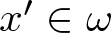 $x'\in {\omega}$
 \begin{equation}
\begin{aligned}
&\int_{{\mathcal{Y}}_1}[E^{(1)}(0,\widehat w^{(1)})]^T{\mathbb{A}}^{(1)}[E^{(1)}(0,\widehat v^{(1)})]\,dy\\
&=-\int_{{\mathcal{Y}}_1}[E^{(1)}({\mathcal{W}}_3^{(1)},0)]^T{\mathbb{A}}^{(1)}[E^{(1)}(0,\widehat v^{(1)})]\,dy\\
&\int_{{\mathcal{Y}}_2}[E^{(2)}(0,\widehat w^{(2)})]^T{\mathbb{A}}^{(2)}[E^{(2)}(0,\widehat v^{(2)})]\,dy\\
&=-\int_{{\mathcal{Y}}_1}[E^{(2)}({\mathcal{W}}_3^{(2)},0)]^T{\mathbb{A}}^{(2)}[E^{(2)}(0,\widehat v^{(2)})]\,dy.
\end{aligned}
\end{equation}
\begin{equation}
\begin{aligned}
&\int_{{\mathcal{Y}}_1}[E^{(1)}(0,\widehat w^{(1)})]^T{\mathbb{A}}^{(1)}[E^{(1)}(0,\widehat v^{(1)})]\,dy\\
&=-\int_{{\mathcal{Y}}_1}[E^{(1)}({\mathcal{W}}_3^{(1)},0)]^T{\mathbb{A}}^{(1)}[E^{(1)}(0,\widehat v^{(1)})]\,dy\\
&\int_{{\mathcal{Y}}_2}[E^{(2)}(0,\widehat w^{(2)})]^T{\mathbb{A}}^{(2)}[E^{(2)}(0,\widehat v^{(2)})]\,dy\\
&=-\int_{{\mathcal{Y}}_1}[E^{(2)}({\mathcal{W}}_3^{(2)},0)]^T{\mathbb{A}}^{(2)}[E^{(2)}(0,\widehat v^{(2)})]\,dy.
\end{aligned}
\end{equation} Observe that to get above equations, we have used that  $L^2\big({\omega};\textbf{L}^2\big((0,1)_{y_\alpha};H^1\big({\mathfrak{I}}^2\big)\big)^3\big)$ is a subspace and varied $t\in{\mathbb{R}}$ and the test functions $\widehat v^{({\alpha})}$.
The equations (7.20) imply that  $\widehat w^{(\alpha)}$ can be expressed in terms of the derivatives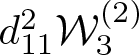 $d^2_{11}{\mathcal{W}}_3^{(2)}$,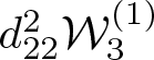 $d^2_{22}{\mathcal{W}}_3^{(1)}$ and some correctors. Let us define the $3\times 3$ symmetric matrices $\textbf{M}^{(1)}$ and $\textbf{M}^{(2)}$
 \begin{align*} &\textbf{M}^{(1)}(y)=\left(\begin{matrix}
0 & * & * \\[1.5mm]
0 & y_3 & *\\[2mm]
0 & \displaystyle {y_2\over 2} & 0
\end{matrix}\right)\quad \hbox{for all } y\in {\mathcal{Y}}_1,\\
& \textbf{M}^{(2)}(y)=\left(\begin{matrix}
y_3 & * & * \\[2mm]
0 & 0 & * \\[2mm]
\displaystyle {y_1\over 2} & 0 & 0
\end{matrix}\right)\quad \hbox{for all } y\in {\mathcal{Y}}_2.\end{align*}
\begin{align*} &\textbf{M}^{(1)}(y)=\left(\begin{matrix}
0 & * & * \\[1.5mm]
0 & y_3 & *\\[2mm]
0 & \displaystyle {y_2\over 2} & 0
\end{matrix}\right)\quad \hbox{for all } y\in {\mathcal{Y}}_1,\\
& \textbf{M}^{(2)}(y)=\left(\begin{matrix}
y_3 & * & * \\[2mm]
0 & 0 & * \\[2mm]
\displaystyle {y_1\over 2} & 0 & 0
\end{matrix}\right)\quad \hbox{for all } y\in {\mathcal{Y}}_2.\end{align*} Due to (7.3) and (7.20), we have  $\widehat w^{(\alpha)}\in L^2\big({\omega}; \textbf{L}^2\big((0,1)_{y_\alpha};H^1\big({\mathfrak{I}}^2\big)\big)^3\big)$ and
 \begin{equation}
\begin{aligned}
\widehat w^{(1)}(x',y)=d^2_{22}{\mathcal{W}}_3^{(1)}(x_2)\widehat \chi^{(1)}(y),\quad \text{a.e. in}\ {\omega}\times {\mathcal{Y}}_1,\\
\widehat w^{(2)}(x',y)=d^2_{11}{\mathcal{W}}_3^{(2)}(x_1)\widehat \chi^{(2)}(y),\quad \text{a.e. in}\ {\omega}\times {\mathcal{Y}}_2,
\end{aligned}
\end{equation}
\begin{equation}
\begin{aligned}
\widehat w^{(1)}(x',y)=d^2_{22}{\mathcal{W}}_3^{(1)}(x_2)\widehat \chi^{(1)}(y),\quad \text{a.e. in}\ {\omega}\times {\mathcal{Y}}_1,\\
\widehat w^{(2)}(x',y)=d^2_{11}{\mathcal{W}}_3^{(2)}(x_1)\widehat \chi^{(2)}(y),\quad \text{a.e. in}\ {\omega}\times {\mathcal{Y}}_2,
\end{aligned}
\end{equation}where  $\widehat \chi^{(\alpha)}\in \textbf{L}^2\big((0,1)_{y_\alpha};H^1\big({\mathfrak{I}}^2\big)\big)^3$ (see (7.1)) are the correctors and they are the solutions to the following cell problems (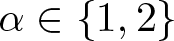 $\alpha\in\{1,2\}$):
 \begin{align}
&\int_{{\mathcal{Y}}_\alpha}\big[E^{(\alpha)}(0,\widehat \chi^{(\alpha)})-\textbf{M}^{(\alpha)}\big]^T{\mathbb{A}}^{(\alpha)}[E^{(\alpha)}(0,\widehat v^{(\alpha)})]\,dy=0, \nonumber\\
& \forall\; \widehat v^{(\alpha)}\in \textbf{L}^2\big((0,1)_{y_\alpha};H^1\big({\mathfrak{I}}^2\big)\big)^3.
\end{align}
\begin{align}
&\int_{{\mathcal{Y}}_\alpha}\big[E^{(\alpha)}(0,\widehat \chi^{(\alpha)})-\textbf{M}^{(\alpha)}\big]^T{\mathbb{A}}^{(\alpha)}[E^{(\alpha)}(0,\widehat v^{(\alpha)})]\,dy=0, \nonumber\\
& \forall\; \widehat v^{(\alpha)}\in \textbf{L}^2\big((0,1)_{y_\alpha};H^1\big({\mathfrak{I}}^2\big)\big)^3.
\end{align} We define the homogenized coefficients in  ${\mathcal{Y}}_\alpha$ as
 \begin{equation}
{\mathcal{C}}^{(\alpha)}_{hom}=\int_{{\mathcal{Y}}_1}\left\langle{\mathbb{A}}^{(\alpha)}[E^{(\alpha)}(0,\widehat \chi^{(\alpha)})-\textbf{M}^{(\alpha)}],[E^{(\alpha)}(0,\widehat \chi^{(\alpha)})-\textbf{M}^{(\alpha)}]\right\rangle\,dy.
\end{equation}
\begin{equation}
{\mathcal{C}}^{(\alpha)}_{hom}=\int_{{\mathcal{Y}}_1}\left\langle{\mathbb{A}}^{(\alpha)}[E^{(\alpha)}(0,\widehat \chi^{(\alpha)})-\textbf{M}^{(\alpha)}],[E^{(\alpha)}(0,\widehat \chi^{(\alpha)})-\textbf{M}^{(\alpha)}]\right\rangle\,dy.
\end{equation}Hence, the limit homogenized energy is given by
 \begin{equation*}
\textbf{J}_{hom}({\mathcal{W}}_3)=\textbf{W}_{hom}({\mathcal{W}}_3)-\int_{\omega} f\cdot {\mathcal{W}}\,dx',
\end{equation*}
\begin{equation*}
\textbf{J}_{hom}({\mathcal{W}}_3)=\textbf{W}_{hom}({\mathcal{W}}_3)-\int_{\omega} f\cdot {\mathcal{W}}\,dx',
\end{equation*}where
 \begin{equation*}
\begin{aligned}
&\textbf{W}_{hom}({\mathcal{W}}_3)=\textbf{W}^{(2)}_{hom}({\mathcal{W}}^{(2)}_3)+\textbf{W}^{(1)}_{hom}({\mathcal{W}}^{(1)}_3),\\
&\textbf{W}^{(2)}_{hom}({\mathcal{W}}^{(2)}_3)=\int_{(0,L)}{\mathcal{C}}^{(2)}_{hom}\,[d^2_{11}{\mathcal{W}}_3^{(2)}]^2\,dx_1,\\ &\textbf{W}^{(1)}_{hom}({\mathcal{W}}^{(1)}_3)=\int_{(0,L)}{\mathcal{C}}^{(1)}_{hom}\,[d^2_{22}{\mathcal{W}}_3^{(1)}]^2\,dx_2.
\end{aligned}
\end{equation*}
\begin{equation*}
\begin{aligned}
&\textbf{W}_{hom}({\mathcal{W}}_3)=\textbf{W}^{(2)}_{hom}({\mathcal{W}}^{(2)}_3)+\textbf{W}^{(1)}_{hom}({\mathcal{W}}^{(1)}_3),\\
&\textbf{W}^{(2)}_{hom}({\mathcal{W}}^{(2)}_3)=\int_{(0,L)}{\mathcal{C}}^{(2)}_{hom}\,[d^2_{11}{\mathcal{W}}_3^{(2)}]^2\,dx_1,\\ &\textbf{W}^{(1)}_{hom}({\mathcal{W}}^{(1)}_3)=\int_{(0,L)}{\mathcal{C}}^{(1)}_{hom}\,[d^2_{22}{\mathcal{W}}_3^{(1)}]^2\,dx_2.
\end{aligned}
\end{equation*}As a consequence of the above set-up, we have
Proposition 7.5. There exist a strictly positive constant  $C_0$ such that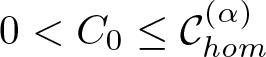 $0 \lt C_0\leq {\mathcal{C}}^{{(\alpha)}}_{hom}$.
Moreover, we have
 \begin{equation*}\textbf{m}=\min\{\textbf{m}^{(1)},\textbf{m}^{(2)}\},\end{equation*}
where
 \begin{equation*}
\begin{aligned}
\textbf{m}^{(1)}&=\inf_{({\mathcal{V}}^{(1)}_3,\widehat v^{(1)})\in {\mathbb{D}}^{(1)}} \Big\{\textbf{W}\big({\mathcal{V}}^{(1)}_3,\widehat v^{(1)},0\big)-\int_{{\omega}} f\cdot\big({\mathcal{V}}_2\textbf{e}_2+{\mathcal{V}}^{(1)}_3\textbf{e}_3\big)\,dx' \Big\}\\
&=\inf_{({\mathcal{V}}^{(1)}_3,\widehat v^{(1)})\in {\mathbb{D}}^{(1)}}\textbf{J}^{(1)}({\mathcal{V}}_3^{(1)},\widehat v^{(1)}),\\
\textbf{m}^{(2)}&=\inf_{({\mathcal{V}}^{(2)}_3,\widehat v^{(2)})\in {\mathbb{D}}^{(2)}} \Big\{\textbf{W}\big({\mathcal{V}}^{(2)}_3,0,\widehat v^{(2)}\big)-\int_{{\omega}} f\cdot\big({\mathcal{V}}_1\textbf{e}_1+{\mathcal{V}}^{(2)}_3\textbf{e}_3\big)\,dx' \Big\}\\
&=\inf_{({\mathcal{V}}^{(2)}_3,\widehat v^{(2)})\in {\mathbb{D}}^{(2)}}\textbf{J}^{(2)}({\mathcal{V}}_3^{(2)},\widehat v^{(2)}),
\end{aligned}
\end{equation*}
\begin{equation*}
\begin{aligned}
\textbf{m}^{(1)}&=\inf_{({\mathcal{V}}^{(1)}_3,\widehat v^{(1)})\in {\mathbb{D}}^{(1)}} \Big\{\textbf{W}\big({\mathcal{V}}^{(1)}_3,\widehat v^{(1)},0\big)-\int_{{\omega}} f\cdot\big({\mathcal{V}}_2\textbf{e}_2+{\mathcal{V}}^{(1)}_3\textbf{e}_3\big)\,dx' \Big\}\\
&=\inf_{({\mathcal{V}}^{(1)}_3,\widehat v^{(1)})\in {\mathbb{D}}^{(1)}}\textbf{J}^{(1)}({\mathcal{V}}_3^{(1)},\widehat v^{(1)}),\\
\textbf{m}^{(2)}&=\inf_{({\mathcal{V}}^{(2)}_3,\widehat v^{(2)})\in {\mathbb{D}}^{(2)}} \Big\{\textbf{W}\big({\mathcal{V}}^{(2)}_3,0,\widehat v^{(2)}\big)-\int_{{\omega}} f\cdot\big({\mathcal{V}}_1\textbf{e}_1+{\mathcal{V}}^{(2)}_3\textbf{e}_3\big)\,dx' \Big\}\\
&=\inf_{({\mathcal{V}}^{(2)}_3,\widehat v^{(2)})\in {\mathbb{D}}^{(2)}}\textbf{J}^{(2)}({\mathcal{V}}_3^{(2)},\widehat v^{(2)}),
\end{aligned}
\end{equation*}with
 \begin{equation*}\begin{aligned}
&{\mathbb{D}}^{(1)}=H_{(0,l)}^{2}\big((0,L)_{x_2}\big)\times {\mathfrak{W}}((0,L)_{x_2}\times {\mathcal{Y}}_1),\\
&{\mathbb{D}}^{(2)}=H_{(0,l)}^{2}\big((0,L)_{x_1}\big)\times {\mathfrak{W}}((0,L)_{x_1}\times {\mathcal{Y}}_2),\\
&{\mathfrak{W}}((0,L)_{x_2}\times {\mathcal{Y}}_1)=\big\{\widehat v^{(1)}\in L^{2}((0,L)_{x_2}\times (0,1)_{y_1};H^1({\mathfrak{I}}^2))^3\;|\; \widehat v^{(1)}=\overline{v}^{(1)}+y_2 Z^{(1)},\\
& \hbox{with}\; \overline{v}^{(1)}\in L^2((0,L)_{x_2}\times (0,1)_{y_1};H^1({\mathfrak{I}}^2))^3\\
&\text{satisfying (7.2)}_1\ \text{and}\ Z^{(1)}\in L^2((0,L)_{x_2})^3 \big\},\\
&{\mathfrak{W}}((0,L)_{x_1}\times {\mathcal{Y}}_2)=\big\{\widehat v^{(2)}\in L^{2}((0,L)_{x_1}\times (0,1)_{y_2};H^1({\mathfrak{I}}^2))^3\;|\;\widehat v^{(2)}=\overline{v}^{(2)}+y_1 Z^{(2)},\\
& \hbox{with}\; \overline{v}^{(2)}\in L^2((0,L)_{x_1}\times (0,1)_{y_2};H^1({\mathfrak{I}}^2))^3\\
& \text{satisfying (7.2)}_2\ \text{and}\ Z^{(2)}\in L^2((0,L)_{x_1})^3\big\},
\end{aligned}
\end{equation*}
\begin{equation*}\begin{aligned}
&{\mathbb{D}}^{(1)}=H_{(0,l)}^{2}\big((0,L)_{x_2}\big)\times {\mathfrak{W}}((0,L)_{x_2}\times {\mathcal{Y}}_1),\\
&{\mathbb{D}}^{(2)}=H_{(0,l)}^{2}\big((0,L)_{x_1}\big)\times {\mathfrak{W}}((0,L)_{x_1}\times {\mathcal{Y}}_2),\\
&{\mathfrak{W}}((0,L)_{x_2}\times {\mathcal{Y}}_1)=\big\{\widehat v^{(1)}\in L^{2}((0,L)_{x_2}\times (0,1)_{y_1};H^1({\mathfrak{I}}^2))^3\;|\; \widehat v^{(1)}=\overline{v}^{(1)}+y_2 Z^{(1)},\\
& \hbox{with}\; \overline{v}^{(1)}\in L^2((0,L)_{x_2}\times (0,1)_{y_1};H^1({\mathfrak{I}}^2))^3\\
&\text{satisfying (7.2)}_1\ \text{and}\ Z^{(1)}\in L^2((0,L)_{x_2})^3 \big\},\\
&{\mathfrak{W}}((0,L)_{x_1}\times {\mathcal{Y}}_2)=\big\{\widehat v^{(2)}\in L^{2}((0,L)_{x_1}\times (0,1)_{y_2};H^1({\mathfrak{I}}^2))^3\;|\;\widehat v^{(2)}=\overline{v}^{(2)}+y_1 Z^{(2)},\\
& \hbox{with}\; \overline{v}^{(2)}\in L^2((0,L)_{x_1}\times (0,1)_{y_2};H^1({\mathfrak{I}}^2))^3\\
& \text{satisfying (7.2)}_2\ \text{and}\ Z^{(2)}\in L^2((0,L)_{x_1})^3\big\},
\end{aligned}
\end{equation*}and 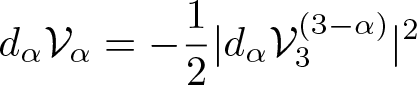 $\displaystyle d_\alpha{\mathcal{V}}_{\alpha}=-{1\over 2}|d_\alpha{\mathcal{V}}_3^{(3-\alpha)}|^2$ a.e. in $(0,L)$,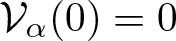 ${\mathcal{V}}_\alpha(0)=0$.
Proof. Since  $\widehat \chi^{(1)}\in \textbf{L}^2\big((0,1)_{y_1};H^1\big({\mathfrak{I}}^2\big)\big)^3$, there exist $\overline{\chi}^{(1)}\in L^2\big((0,1)_{y_1};H^1\big({\mathfrak{I}}^2\big)\big)^3$ satisfying (7.2) $_1$ and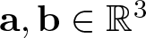 $\textbf{a},\textbf{b}\in{\mathbb{R}}^3$ such that
 \begin{equation*}\widehat \chi^{(1)}(y)=\overline{\chi}^{(1)}(y)+\textbf{a} y_2+\textbf{b} y_1 y_2,\quad \forall\,y\in {\mathcal{Y}}_1.\end{equation*}
Let us set (see (A.8))
 \begin{equation*}\widetilde {\chi}^{(1)}(y)= \overline{\chi}^{(1)}(y)+\textbf{a} y_2+\textbf{b} y_1 y_2-y_2 y_3\textbf{e}_3,\quad \forall\,y\in {\mathcal{Y}}_1,\end{equation*}
then, using (7.4) and (7.13), we get
 \begin{equation*}\begin{aligned}
{\mathcal{C}}^{(1)}_{hom}\geq c_0\|E^{(1)}(0,\widehat \chi^{(1)})-\textbf{M}^{(1)}\|^2_{L^2({\mathcal{Y}}_1)}= c_0\|E^{(1)}(0,\widetilde \chi^{(1)})\|^2_{L^2({\mathcal{Y}}_1)}\\
\geq c_0\big(1+|\textbf{a}|^2+|\textbf{b}|^2+\|\overline{\chi}^{(1)}\|^2_{L^2((0,1)_{y_1};H^1({\mathfrak{I}}^2)}\big)=C_1 \gt 0.
\end{aligned}
\end{equation*}
\begin{equation*}\begin{aligned}
{\mathcal{C}}^{(1)}_{hom}\geq c_0\|E^{(1)}(0,\widehat \chi^{(1)})-\textbf{M}^{(1)}\|^2_{L^2({\mathcal{Y}}_1)}= c_0\|E^{(1)}(0,\widetilde \chi^{(1)})\|^2_{L^2({\mathcal{Y}}_1)}\\
\geq c_0\big(1+|\textbf{a}|^2+|\textbf{b}|^2+\|\overline{\chi}^{(1)}\|^2_{L^2((0,1)_{y_1};H^1({\mathfrak{I}}^2)}\big)=C_1 \gt 0.
\end{aligned}
\end{equation*} Similarly, we get 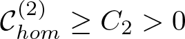 $\mathcal{C}^{(2)}_{hom}\geq C_2 \gt 0$. Taking $C_0=\min\{C_1,C_2\}$ gives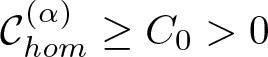 $\mathcal{C}^{(\alpha)}_{hom}\geq C_0 \gt 0$.
First observe that, proceeding as in the proof of Proposition 7.4, there exists a minimizer of  $\textbf{J}^{(\alpha)}$ in ${\mathbb{D}}^{(\alpha)}$ and $\textbf{m}^{(\alpha)}$ is in fact a minimum by the sequential criterion.
From Proposition 7.4, we have (since 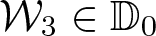 ${\mathcal{W}}_3\in {\mathbb{D}}_0$, we have ${\mathcal{W}}_3={\mathcal{W}}_3^{(2)}+{\mathcal{W}}_3^{(1)}$ and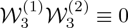 ${\mathcal{W}}_3^{(1)}{\mathcal{W}}_3^{(2)}\equiv0$ a.e. in $(0,L)$ with ${\mathcal{W}}_3^{(3-\alpha)}\in H_{(0,l)}^{2}((0,L)_{x_\alpha})$)
 \begin{equation*}\textbf{J}({\mathcal{W}}_3,\widehat w^{(1)},\widehat w^{(2)})= \textbf{m}
= \inf_{({\mathcal{U}}_{3},\widehat v^{(1)},\widehat v^{(2)})\in {\mathbb{D}}}\textbf{J}({\mathcal{U}}_3,\widehat v^{(1)},\widehat v^{(2)}).\end{equation*}
\begin{equation*}\textbf{J}({\mathcal{W}}_3,\widehat w^{(1)},\widehat w^{(2)})= \textbf{m}
= \inf_{({\mathcal{U}}_{3},\widehat v^{(1)},\widehat v^{(2)})\in {\mathbb{D}}}\textbf{J}({\mathcal{U}}_3,\widehat v^{(1)},\widehat v^{(2)}).\end{equation*} Without loss of generality, let us assume 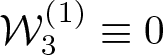 ${\mathcal{W}}_3^{(1)}\equiv0$, which using (7.21) $_1$ gives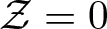 ${\mathcal{Z}}=0$, a.e. in ${\omega}$. Then, using (7.21), we have
 \begin{align*}\textbf{m}&=\textbf{J}({\mathcal{W}}^{(2)}_3,0,\widehat w^{(2)})=\textbf{W}\big({\mathcal{W}}^{(2)}_3,0,\widehat w^{(2)}\big)\\
&\quad -\int_{{\omega}} f\cdot\big({\mathcal{W}}_1\textbf{e}_1+{\mathcal{W}}^{(2)}_3\textbf{e}_3\big)\,dx'=\textbf{J}^{(2)}({\mathcal{W}}_3^{(2)},\widehat w^{(2)}) ,\end{align*}
\begin{align*}\textbf{m}&=\textbf{J}({\mathcal{W}}^{(2)}_3,0,\widehat w^{(2)})=\textbf{W}\big({\mathcal{W}}^{(2)}_3,0,\widehat w^{(2)}\big)\\
&\quad -\int_{{\omega}} f\cdot\big({\mathcal{W}}_1\textbf{e}_1+{\mathcal{W}}^{(2)}_3\textbf{e}_3\big)\,dx'=\textbf{J}^{(2)}({\mathcal{W}}_3^{(2)},\widehat w^{(2)}) ,\end{align*}where  $d_1{\mathcal{W}}_1=-{1\over 2}|d_1{\mathcal{W}}_3^{(2)}|^2$ a.e. in $(0,L)$. So, we have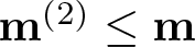 $\textbf{m}^{(2)}\leq \textbf{m}$, since $({\mathcal{W}}_3^{(2)},\widehat w^{(2)})\in{\mathbb{D}}^{(2)}$.
On the other hand, since  $({\mathcal{W}}_3^{(2)},0,\widehat w^{(2)})\in {\mathbb{D}}$, we have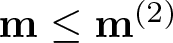 $\textbf{m}\leq \textbf{m}^{(2)}$. Finally, we have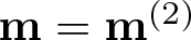 $\textbf{m}=\textbf{m}^{(2)}$.
Similarly, if we assume 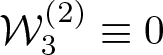 ${\mathcal{W}}_3^{(2)}\equiv0$, which using (7.21) $_2$ gives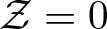 ${\mathcal{Z}}=0$ a.e. in ${\omega}$. Then analogously we obtain
 \begin{align*}\textbf{m}&=\textbf{J}({\mathcal{W}}_3^{(1)},\widehat w^{(1)},0)=\textbf{W}\big({\mathcal{W}}^{(1)}_3,\widehat w^{(1)},0\big)-\int_{{\omega}} f\cdot\big({\mathcal{W}}_2\textbf{e}_2+{\mathcal{W}}^{(1)}_3\textbf{e}_3\big)\,dx'\\
&=\textbf{m}^{(1)}=\textbf{J}^{(1)}({\mathcal{W}}_3^{(1)},\widehat w^{(1)}).\end{align*}
\begin{align*}\textbf{m}&=\textbf{J}({\mathcal{W}}_3^{(1)},\widehat w^{(1)},0)=\textbf{W}\big({\mathcal{W}}^{(1)}_3,\widehat w^{(1)},0\big)-\int_{{\omega}} f\cdot\big({\mathcal{W}}_2\textbf{e}_2+{\mathcal{W}}^{(1)}_3\textbf{e}_3\big)\,dx'\\
&=\textbf{m}^{(1)}=\textbf{J}^{(1)}({\mathcal{W}}_3^{(1)},\widehat w^{(1)}).\end{align*}Consequently,
 \begin{equation*}\textbf{m}=\textbf{m}^{(1)} \quad\text{or}\quad \textbf{m}=\textbf{m}^{(2)}.\end{equation*}
Using the homogenized coefficients (7.23), we have
 \begin{equation*}\begin{aligned}
\textbf{m}^{(1)}&=\textbf{J}^{(1)}({\mathcal{W}}_3^{(1)},\widehat w^{(1)})=\int_{(0,L)}{\mathcal{C}}^{(1)}_{hom}\,[d^2_{22}{\mathcal{W}}_3^{(1)}]^2\,dx_2\\
&\quad -\int_{{\omega}} f\cdot\big({\mathcal{W}}_2\textbf{e}_2+{\mathcal{W}}^{(1)}_3\textbf{e}_3\big)\,dx'=\textbf{J}^{(1)}_{hom}({\mathcal{W}}_3^{(1)}),\\
\textbf{m}^{(2)}&=\textbf{J}^{(2)}({\mathcal{W}}_3^{(2)},\widehat w^{(2)})=\int_{(0,L)}{\mathcal{C}}^{(2)}_{hom}\,[d^2_{11}{\mathcal{W}}_3^{(2)}]^2\,dx_1\\
&\quad -\int_{{\omega}} f\cdot\big({\mathcal{W}}_1\textbf{e}_1+{\mathcal{W}}^{(1)}_3\textbf{e}_3\big)\,dx'=\textbf{J}^{(2)}_{hom}({\mathcal{W}}_3^{(2)}),
\end{aligned}
\end{equation*}
\begin{equation*}\begin{aligned}
\textbf{m}^{(1)}&=\textbf{J}^{(1)}({\mathcal{W}}_3^{(1)},\widehat w^{(1)})=\int_{(0,L)}{\mathcal{C}}^{(1)}_{hom}\,[d^2_{22}{\mathcal{W}}_3^{(1)}]^2\,dx_2\\
&\quad -\int_{{\omega}} f\cdot\big({\mathcal{W}}_2\textbf{e}_2+{\mathcal{W}}^{(1)}_3\textbf{e}_3\big)\,dx'=\textbf{J}^{(1)}_{hom}({\mathcal{W}}_3^{(1)}),\\
\textbf{m}^{(2)}&=\textbf{J}^{(2)}({\mathcal{W}}_3^{(2)},\widehat w^{(2)})=\int_{(0,L)}{\mathcal{C}}^{(2)}_{hom}\,[d^2_{11}{\mathcal{W}}_3^{(2)}]^2\,dx_1\\
&\quad -\int_{{\omega}} f\cdot\big({\mathcal{W}}_1\textbf{e}_1+{\mathcal{W}}^{(1)}_3\textbf{e}_3\big)\,dx'=\textbf{J}^{(2)}_{hom}({\mathcal{W}}_3^{(2)}),
\end{aligned}
\end{equation*}so, we have
 \begin{equation*}\textbf{m}=\min\{\textbf{m}^{(1)},\textbf{m}^{(2)}\}.\end{equation*}
This completes the proof.
7.4. Construction of the recovery sequence
In this section, we construct the sequence of test deformations.
Proposition 7.6. We have
 \begin{equation}
\limsup_{(\varepsilon,\delta)\to(0,0)}{\textbf{m}_{\varepsilon\delta}\over \varepsilon^2\delta^3}\leq \textbf{m}.
\end{equation}
\begin{equation}
\limsup_{(\varepsilon,\delta)\to(0,0)}{\textbf{m}_{\varepsilon\delta}\over \varepsilon^2\delta^3}\leq \textbf{m}.
\end{equation}Proof. Below, we assume that 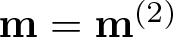 $\textbf{m}=\textbf{m}^{(2)}$, and we show that
 \begin{equation*}\limsup_{(\varepsilon,\delta)\to(0,0)}{\textbf{m}_{\varepsilon\delta}\over \varepsilon^2\delta^3}\leq \textbf{m}^{(2)}.\end{equation*}
 The proof in the case 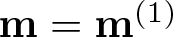 $\textbf{m}= \textbf{m}^{(1)}$ is similar. In Proposition 7.5, we obtained that $\textbf{m}^{(2)}$ is the minimum of the functional $\textbf{J}^{(2)}$ over the space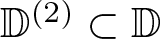 ${\mathbb{D}}^{(2)}\subset {\mathbb{D}}$.
In the following, for the sake of simplicity, we omit the superscript  $\phantom{A}^{(2)}$ in the test functions but use the superscript for the unfolding operators and spaces.
That is why we start with 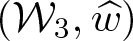 $({\mathcal{W}}_3,\widehat w)$ an element in ${\mathbb{D}}^{(2)}\cap\big( \mathcal{C}^2([0,L]_{x_1})\times \mathcal{C}^1([0,L]_{x_1}\times \overline{{\mathcal{Y}}_2})^3\big)$, $\widehat w$ with compact support with respect to $x_1$.
We define  ${\mathcal{W}}_1\in H_{(0,l)}^{1}\big((0,L)_{x_1}\big)\cap \mathcal{C}^1([0,L])$ as
 \begin{equation*}d_1{\mathcal{W}}_1=-{1\over 2}\big|d_1{\mathcal{W}}_3\big|^2,\quad\text{in}\ (0,L),\end{equation*}
and
 \begin{align*}
&{\mathcal{W}}(x')={\mathcal{W}}_{1}(x_1)\textbf{e}_1+{\mathcal{W}}_{3}(x_1)\textbf{e}_3,\\ &\textbf{A}(x_1)=\left(\begin{matrix}
0&0&-d_1{\mathcal{W}}_3(x_1)\\
0&0&0\\
d_1{\mathcal{W}}_3(x_1)&0&0
\end{matrix}\right),\quad\text{for}\ x'\in{\omega}.\end{align*}
\begin{align*}
&{\mathcal{W}}(x')={\mathcal{W}}_{1}(x_1)\textbf{e}_1+{\mathcal{W}}_{3}(x_1)\textbf{e}_3,\\ &\textbf{A}(x_1)=\left(\begin{matrix}
0&0&-d_1{\mathcal{W}}_3(x_1)\\
0&0&0\\
d_1{\mathcal{W}}_3(x_1)&0&0
\end{matrix}\right),\quad\text{for}\ x'\in{\omega}.\end{align*}We also have
 \begin{equation}
\widehat w=\overline{w}+y_1 Z\in {\mathfrak{W}}((0,L)_{x_1}\times {\mathcal{Y}}_2) \cap \mathcal{C}^1([0,L]_{x_1}\times \overline{{\mathcal{Y}}_2})^3.
\end{equation}
\begin{equation}
\widehat w=\overline{w}+y_1 Z\in {\mathfrak{W}}((0,L)_{x_1}\times {\mathcal{Y}}_2) \cap \mathcal{C}^1([0,L]_{x_1}\times \overline{{\mathcal{Y}}_2})^3.
\end{equation} Due to (7.21), we can take 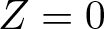 $Z=0$ a.e. in $(0,l)$.
Step 1. In this step, to any function  $\psi\in H^1\big((0,L)_{x_1})$, we associate $\displaystyle \psi^{\diamond}_{\varepsilon\delta}\in H^1\Big(\Big(-{\delta\over 2},L+{\delta\over 2}\Big)_{x_1}\Big)$.
First we extend  $\psi$ by setting (the extension of $\psi$ is still denoted $\psi$)
 \begin{equation*}
\psi(x_1)=\psi(0)\qquad \forall x_1\in \Big[-{\delta\over 2},0\Big],\qquad \psi(x_1)=\psi(L)\qquad \forall x_1\in \Big[L,L+{\delta\over 2}\Big].
\end{equation*}
\begin{equation*}
\psi(x_1)=\psi(0)\qquad \forall x_1\in \Big[-{\delta\over 2},0\Big],\qquad \psi(x_1)=\psi(L)\qquad \forall x_1\in \Big[L,L+{\delta\over 2}\Big].
\end{equation*} Then, we define the function  $\psi^{\diamond}_{\varepsilon\delta}$ by
 \begin{equation}
\psi^{\diamond}_{\varepsilon\delta}(x_1)=\left\{\begin{aligned}
&\psi\Big(p\varepsilon+{\varepsilon\over \delta}z_1\Big),\quad&& x_1=p\varepsilon+z_1,\quad z_1\in{\mathfrak{I}}_\delta,\quad p\in\{0,\ldots,N_\varepsilon\},\\
&\psi\Big(p\varepsilon+{\varepsilon\over 2}\Big) ,\quad && x_1\in(p\varepsilon+{\delta\over 2},p\varepsilon+\varepsilon-{\delta\over 2}),\quad p\in\{0,\ldots,N_\varepsilon-1\}.
\end{aligned}
\right.
\end{equation}
\begin{equation}
\psi^{\diamond}_{\varepsilon\delta}(x_1)=\left\{\begin{aligned}
&\psi\Big(p\varepsilon+{\varepsilon\over \delta}z_1\Big),\quad&& x_1=p\varepsilon+z_1,\quad z_1\in{\mathfrak{I}}_\delta,\quad p\in\{0,\ldots,N_\varepsilon\},\\
&\psi\Big(p\varepsilon+{\varepsilon\over 2}\Big) ,\quad && x_1\in(p\varepsilon+{\delta\over 2},p\varepsilon+\varepsilon-{\delta\over 2}),\quad p\in\{0,\ldots,N_\varepsilon-1\}.
\end{aligned}
\right.
\end{equation}Note that
 \begin{align}
&d_1\psi^{\diamond}_{\varepsilon\delta}(x_1) \nonumber\\
&=\left\{\begin{aligned}
&{\varepsilon\over \delta}d_1\psi\Big(p\varepsilon+{\varepsilon\over \delta}z_1\Big),\quad&& x_1=p\varepsilon+z_1,\quad z_1\in{\mathfrak{I}}_\delta,\quad p\in\{0,\ldots,N_\varepsilon\},\\
&0 ,\quad && x_1\in(p\varepsilon+{\delta\over 2},p\varepsilon+\varepsilon-{\delta\over 2}),\quad p\in\{0,\ldots,N_\varepsilon-1\}.
\end{aligned}
\right.
\end{align}
\begin{align}
&d_1\psi^{\diamond}_{\varepsilon\delta}(x_1) \nonumber\\
&=\left\{\begin{aligned}
&{\varepsilon\over \delta}d_1\psi\Big(p\varepsilon+{\varepsilon\over \delta}z_1\Big),\quad&& x_1=p\varepsilon+z_1,\quad z_1\in{\mathfrak{I}}_\delta,\quad p\in\{0,\ldots,N_\varepsilon\},\\
&0 ,\quad && x_1\in(p\varepsilon+{\delta\over 2},p\varepsilon+\varepsilon-{\delta\over 2}),\quad p\in\{0,\ldots,N_\varepsilon-1\}.
\end{aligned}
\right.
\end{align} Step 2. In this step, we construct the sequence of admissible deformations  $\{w_{{\varepsilon\delta}}\}_{\varepsilon,\delta}\subset \textbf{V}_{\varepsilon\delta}$.
The sequence of test deformations  $w_{\varepsilon\delta}$ is
 \begin{equation*}w_{{\varepsilon\delta}}=I_d+U_{e,{\varepsilon\delta}}+\overline{w}_{\varepsilon\delta}\qquad \hbox{in}\;\; \Omega_\delta\end{equation*}
where
 \begin{align*}
&\overline{w}_{{\varepsilon\delta}}(p\varepsilon+\delta y_1,q\varepsilon+\varepsilon y_2,\delta y_3)= ({\varepsilon\delta})^{3/2}\overline{w}(p\varepsilon,q\varepsilon, y)\\
&\quad \text{for a.e.}\ y\in {\mathcal{Y}}_2\ \text{and for all}\ (p,q)\in {\mathcal{K}}_\varepsilon
\end{align*}
\begin{align*}
&\overline{w}_{{\varepsilon\delta}}(p\varepsilon+\delta y_1,q\varepsilon+\varepsilon y_2,\delta y_3)= ({\varepsilon\delta})^{3/2}\overline{w}(p\varepsilon,q\varepsilon, y)\\
&\quad \text{for a.e.}\ y\in {\mathcal{Y}}_2\ \text{and for all}\ (p,q)\in {\mathcal{K}}_\varepsilon
\end{align*}and 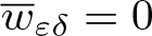 $\overline{w}_{{\varepsilon\delta}}=0$ a.e. in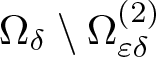 $\Omega_\delta\setminus{\Omega^{(2)}_{\varepsilon\delta}}$.
The field  $U_{e,{\varepsilon\delta}}$ is defined as follows: In $\Omega_\delta$ by
 \begin{equation}
\begin{aligned}
U_{e,{\varepsilon\delta}}(x)={\mathcal{W}}_{{\varepsilon\delta}}(x_1)+\int_{-{\delta\over 2}}^{x_1}(\textbf{R}^{\diamond}_{{\varepsilon\delta}}(t)-\textbf{I}_3)\textbf{e}_1\,dt
+(\textbf{R}^{\diamond}_{{\varepsilon\delta}}(x_1)-\textbf{I}_3)x_3\textbf{e}_3,
\end{aligned}
\end{equation}
\begin{equation}
\begin{aligned}
U_{e,{\varepsilon\delta}}(x)={\mathcal{W}}_{{\varepsilon\delta}}(x_1)+\int_{-{\delta\over 2}}^{x_1}(\textbf{R}^{\diamond}_{{\varepsilon\delta}}(t)-\textbf{I}_3)\textbf{e}_1\,dt
+(\textbf{R}^{\diamond}_{{\varepsilon\delta}}(x_1)-\textbf{I}_3)x_3\textbf{e}_3,
\end{aligned}
\end{equation}where the field of matrices  $\textbf{R}_{\varepsilon\delta}^{\diamond} \in \displaystyle W^{1,\infty}\Big(\Big(-{\delta\over 2},L+{\delta\over 2}\Big)_{x_1}; \mathrm{SO}(3)\Big)$ is constructed using Step 1 by transforming $\textbf{R}_{\varepsilon\delta}\in \mathcal{C}^1([0,L]_{x_1};\mathrm{SO}(3))$, defined by
 \begin{equation*}\textbf{R}_{{\varepsilon\delta}}(x_1)= \exp\big(\sqrt{{\varepsilon\delta}}\textbf{A}(x_1)\big),\qquad x_1\in(0,L).\end{equation*}
 Observe that  $(\textbf{R}_{\varepsilon\delta}-\textbf{I}_3)\textbf{e}_2=0$ in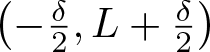 $\left(-{\delta\over 2},L+{\delta\over 2}\right)$. The field $\displaystyle {\mathcal{W}}_{\varepsilon\delta}\in W^{1,\infty}\Big(\Big(-{\delta\over 2},L+{\delta\over 2}\Big)_{x_1}\Big)^3$ is defined by
 \begin{equation}
{\mathcal{W}}_{\varepsilon\delta}={\varepsilon\delta} W_{\varepsilon\delta}+\delta\sqrt{{\varepsilon\delta}}\textbf{Z}_{\varepsilon\delta}^{\diamond}\qquad \hbox{a.e. in }\; (-{\delta\over2},L+{\delta\over2})
\end{equation}
\begin{equation}
{\mathcal{W}}_{\varepsilon\delta}={\varepsilon\delta} W_{\varepsilon\delta}+\delta\sqrt{{\varepsilon\delta}}\textbf{Z}_{\varepsilon\delta}^{\diamond}\qquad \hbox{a.e. in }\; (-{\delta\over2},L+{\delta\over2})
\end{equation}where  $\textbf{Z}^{\diamond}_{\varepsilon\delta}$ is constructed as in Step 1 by transforming
 \begin{equation}
\textbf{Z}(x_1)=\int_0^{x_1}Z(t)\,dt,\quad x_1\in[0,L],
\end{equation}
\begin{equation}
\textbf{Z}(x_1)=\int_0^{x_1}Z(t)\,dt,\quad x_1\in[0,L],
\end{equation}  $ W_{\varepsilon\delta}$ is given by
 \begin{equation}
\begin{aligned}
{W}_{\varepsilon\delta} (x_1)&={4(x_1-p\varepsilon)^2-\delta^2\over 8\delta^2}d_1\textbf{R}_{\varepsilon\delta}^{\diamond}(p\varepsilon)\textbf{e}_1\qquad x_1\in p\varepsilon+{\mathfrak{I}}_\delta,\qquad p\in \big\{0,\ldots,N_\varepsilon\big\},\\
{W}_{\varepsilon\delta} (x_1)&=0\hskip 30mm x_1\in \Big(p\varepsilon+{\delta\over 2},p\varepsilon+\varepsilon-{\delta\over 2}\Big)\qquad p\in \big\{0,\ldots,N_\varepsilon-1\big\}.
\end{aligned}
\end{equation}
\begin{equation}
\begin{aligned}
{W}_{\varepsilon\delta} (x_1)&={4(x_1-p\varepsilon)^2-\delta^2\over 8\delta^2}d_1\textbf{R}_{\varepsilon\delta}^{\diamond}(p\varepsilon)\textbf{e}_1\qquad x_1\in p\varepsilon+{\mathfrak{I}}_\delta,\qquad p\in \big\{0,\ldots,N_\varepsilon\big\},\\
{W}_{\varepsilon\delta} (x_1)&=0\hskip 30mm x_1\in \Big(p\varepsilon+{\delta\over 2},p\varepsilon+\varepsilon-{\delta\over 2}\Big)\qquad p\in \big\{0,\ldots,N_\varepsilon-1\big\}.
\end{aligned}
\end{equation} So, by construction, we have  $w_{{\varepsilon\delta}}\in H^1(\Omega_\delta)^3$ and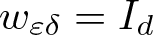 $w_{{\varepsilon\delta}}=I_d$ a.e. on $\Gamma_\delta$ due to the boundary condition satisfied by ${\mathcal{W}}_3$ since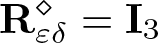 $\textbf{R}_{\varepsilon\delta}^{\diamond}=\textbf{I}_3$ in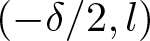 $(-\delta/2,l)$ (due the boundary condition satisfied by $\textbf{A}$) which in turn give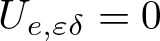 $U_{e,{\varepsilon\delta}}=0$ on $\Gamma_\delta$.
Due to (7.28), we have the following:
 \begin{equation*}
\nabla U_{e,{\varepsilon\delta}}-(\textbf{R}_{\varepsilon\delta}^{\diamond}-\textbf{I}_3)=0, \quad\text{a.e. in } \Omega^H_{pq},\quad (p,q)\in{\mathcal{K}}_\varepsilon^*
\end{equation*}
\begin{equation*}
\nabla U_{e,{\varepsilon\delta}}-(\textbf{R}_{\varepsilon\delta}^{\diamond}-\textbf{I}_3)=0, \quad\text{a.e. in } \Omega^H_{pq},\quad (p,q)\in{\mathcal{K}}_\varepsilon^*
\end{equation*}since (see (7.29)–(7.30) and (7.27))
 \begin{equation*}
\begin{aligned}
d_1{\mathcal{W}}_{\varepsilon\delta}(x_1)&=0,\quad x_1\in \Big(p\varepsilon+{\delta\over 2},p\varepsilon+\varepsilon-{\delta\over 2}\Big),\, p\in \big\{0,\ldots,N_\varepsilon-1\big\},\\
d_1{\mathcal{W}}_{\varepsilon\delta}(x_1)&={\varepsilon\delta} d_1 W_{\varepsilon\delta}+\delta\sqrt{{\varepsilon\delta}}\,d_1\textbf{Z}^{\diamond}_{\varepsilon\delta}, \qquad x_1\in p\varepsilon+{\mathfrak{I}}_\delta,\quad p\in \big\{0,\ldots,N_\varepsilon\big\}.
\end{aligned}
\end{equation*}
\begin{equation*}
\begin{aligned}
d_1{\mathcal{W}}_{\varepsilon\delta}(x_1)&=0,\quad x_1\in \Big(p\varepsilon+{\delta\over 2},p\varepsilon+\varepsilon-{\delta\over 2}\Big),\, p\in \big\{0,\ldots,N_\varepsilon-1\big\},\\
d_1{\mathcal{W}}_{\varepsilon\delta}(x_1)&={\varepsilon\delta} d_1 W_{\varepsilon\delta}+\delta\sqrt{{\varepsilon\delta}}\,d_1\textbf{Z}^{\diamond}_{\varepsilon\delta}, \qquad x_1\in p\varepsilon+{\mathfrak{I}}_\delta,\quad p\in \big\{0,\ldots,N_\varepsilon\big\}.
\end{aligned}
\end{equation*} So, we have  $\nabla w_{\varepsilon\delta}\in \mathrm{SO}(3)$ a.e. in $\Omega^H_{\varepsilon\delta}$. This implies $w_{\varepsilon\delta}\in \textbf{V}_{\varepsilon\delta}$.
Step 3. In this step, we give convergence of the fields.
Observe that
 \begin{equation}
{1\over ({\varepsilon\delta})^{3/2}}\Pi_{\varepsilon\delta}(\overline{w}_{\varepsilon\delta}) \to \overline{w}\quad \text{strongly in}\ L^2\big({\omega}\times (0,1)_{y_2};H^1({\mathfrak{I}}^2)\big)^3.
\end{equation}
\begin{equation}
{1\over ({\varepsilon\delta})^{3/2}}\Pi_{\varepsilon\delta}(\overline{w}_{\varepsilon\delta}) \to \overline{w}\quad \text{strongly in}\ L^2\big({\omega}\times (0,1)_{y_2};H^1({\mathfrak{I}}^2)\big)^3.
\end{equation} Recalling  $\textbf{A}$ belongs to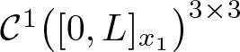 ${\mathcal{C}}^1\big([0,L]_{x_1}\big)^{3\times 3}$ and is uniformly bounded in this space. Since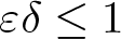 ${\varepsilon\delta}\leq 1$, the classical properties of the exponential of a matrix yield
 \begin{equation}
\begin{aligned}
&\big\|\textbf{R}_{\varepsilon\delta}-\textbf{I}_3\big\|_{L^\infty(0,L)}\leq \sqrt{{\varepsilon\delta}}\|\textbf{A}\|_{L^\infty(0,L)}\exp\big(\|\textbf{A}\|_{L^\infty(0,L)}\big)\leq C\sqrt{{\varepsilon\delta}},\\
&\big\|\textbf{R}_{\varepsilon\delta}-\textbf{I}_3-\sqrt{{\varepsilon\delta}}\textbf{A}\big\|_{L^\infty(0,L)}\leq {\varepsilon\delta}\|\textbf{A}\|^2_{L^\infty(0,L)}\exp\big(\|\textbf{A}\|_{L^\infty(0,L)}\big)\leq C {\varepsilon\delta},\\
& \Big\|\textbf{R}_{\varepsilon\delta}-\textbf{I}_3-\sqrt{{\varepsilon\delta}}\textbf{A}-{{\varepsilon\delta}\over 2} \textbf{A}^2\Big\|_{L^\infty(0,L)}\leq ({\varepsilon\delta})^{3/2}\|\textbf{A}\|^3_{L^\infty(0,L)}\exp\big(\|\textbf{A}\|_{L^\infty(0,L)}\big)\\
&\leq C ({\varepsilon\delta})^{3/2},\\
&\big\|d_1\textbf{R}_{\varepsilon\delta}-\sqrt{{\varepsilon\delta}}\,d_1\textbf{A}\big\|_{L^\infty(0,L)}\leq {\varepsilon\delta}\|d_1\textbf{A}\|_{L^\infty(0,L)}\|\textbf{A}\|_{L^\infty(0,L)} \exp\big(\|\textbf{A}\|_{L^\infty(0,L)}\big)\leq C{\varepsilon\delta}.
\end{aligned}
\end{equation}
\begin{equation}
\begin{aligned}
&\big\|\textbf{R}_{\varepsilon\delta}-\textbf{I}_3\big\|_{L^\infty(0,L)}\leq \sqrt{{\varepsilon\delta}}\|\textbf{A}\|_{L^\infty(0,L)}\exp\big(\|\textbf{A}\|_{L^\infty(0,L)}\big)\leq C\sqrt{{\varepsilon\delta}},\\
&\big\|\textbf{R}_{\varepsilon\delta}-\textbf{I}_3-\sqrt{{\varepsilon\delta}}\textbf{A}\big\|_{L^\infty(0,L)}\leq {\varepsilon\delta}\|\textbf{A}\|^2_{L^\infty(0,L)}\exp\big(\|\textbf{A}\|_{L^\infty(0,L)}\big)\leq C {\varepsilon\delta},\\
& \Big\|\textbf{R}_{\varepsilon\delta}-\textbf{I}_3-\sqrt{{\varepsilon\delta}}\textbf{A}-{{\varepsilon\delta}\over 2} \textbf{A}^2\Big\|_{L^\infty(0,L)}\leq ({\varepsilon\delta})^{3/2}\|\textbf{A}\|^3_{L^\infty(0,L)}\exp\big(\|\textbf{A}\|_{L^\infty(0,L)}\big)\\
&\leq C ({\varepsilon\delta})^{3/2},\\
&\big\|d_1\textbf{R}_{\varepsilon\delta}-\sqrt{{\varepsilon\delta}}\,d_1\textbf{A}\big\|_{L^\infty(0,L)}\leq {\varepsilon\delta}\|d_1\textbf{A}\|_{L^\infty(0,L)}\|\textbf{A}\|_{L^\infty(0,L)} \exp\big(\|\textbf{A}\|_{L^\infty(0,L)}\big)\leq C{\varepsilon\delta}.
\end{aligned}
\end{equation} The above estimates along with the fact that (recall that 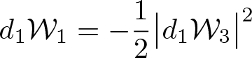 $\displaystyle d_1{\mathcal{W}}_1=-{1\over 2}\big|d_1{\mathcal{W}}_3\big|^2$)
 \begin{equation*}
\begin{aligned}
& \textbf{A}\textbf{e}_1\cdot\textbf{e}_1=0,\qquad \textbf{A}\textbf{e}_1\cdot\textbf{e}_3=d_1{\mathcal{W}}_3,\qquad \textbf{A}^2\textbf{e}_1\cdot\textbf{e}_1=2d_1{\mathcal{W}}_1
\end{aligned}
\end{equation*}
\begin{equation*}
\begin{aligned}
& \textbf{A}\textbf{e}_1\cdot\textbf{e}_1=0,\qquad \textbf{A}\textbf{e}_1\cdot\textbf{e}_3=d_1{\mathcal{W}}_3,\qquad \textbf{A}^2\textbf{e}_1\cdot\textbf{e}_1=2d_1{\mathcal{W}}_1
\end{aligned}
\end{equation*}give the following convergences:
 \begin{equation}
\begin{aligned}
\textbf{R}_{\varepsilon\delta} & \to \textbf{I}_3\quad &&\text{strongly in}\ H^1(0,L)^{3\times 3},\\
{1\over \sqrt{{\varepsilon\delta}}}(\textbf{R}_{\varepsilon\delta}-\textbf{I}_3) & \to \textbf{A}\quad &&\text{strongly in}\ H^1(0,L)^{3\times 3},\\
{1\over \sqrt{{\varepsilon\delta}}}(\textbf{R}_{\varepsilon\delta}-\textbf{I}_3)\textbf{e}_1\cdot\textbf{e}_3&\to d_1 {\mathcal{W}}_3\quad &&\text{strongly in}\ L^2(0,L),\\
{1\over {\varepsilon\delta}}(\textbf{R}_{\varepsilon\delta}-\textbf{I}_3)\textbf{e}_1\cdot\textbf{e}_1&\to d_1 {\mathcal{W}}_1\quad &&\text{strongly in}\ L^2(0,L).
\end{aligned}
\end{equation}
\begin{equation}
\begin{aligned}
\textbf{R}_{\varepsilon\delta} & \to \textbf{I}_3\quad &&\text{strongly in}\ H^1(0,L)^{3\times 3},\\
{1\over \sqrt{{\varepsilon\delta}}}(\textbf{R}_{\varepsilon\delta}-\textbf{I}_3) & \to \textbf{A}\quad &&\text{strongly in}\ H^1(0,L)^{3\times 3},\\
{1\over \sqrt{{\varepsilon\delta}}}(\textbf{R}_{\varepsilon\delta}-\textbf{I}_3)\textbf{e}_1\cdot\textbf{e}_3&\to d_1 {\mathcal{W}}_3\quad &&\text{strongly in}\ L^2(0,L),\\
{1\over {\varepsilon\delta}}(\textbf{R}_{\varepsilon\delta}-\textbf{I}_3)\textbf{e}_1\cdot\textbf{e}_1&\to d_1 {\mathcal{W}}_1\quad &&\text{strongly in}\ L^2(0,L).
\end{aligned}
\end{equation} Due to the definitions of  $\mathcal{T}_{\varepsilon\delta}^{(2)}$ (see (5.4)) and (7.26), we have
 \begin{equation*}
\begin{aligned}
\mathcal{T}_{\varepsilon\delta}^{(2)}(\textbf{R}_{\varepsilon\delta}^{\diamond})(x_1,x_2,y_1,y_2) &=\textbf{R}_{\varepsilon\delta}\big(p\varepsilon+\delta y_1\big)\quad (x_1, y_1)\in [p\varepsilon,p\varepsilon+\varepsilon)\times {\mathfrak{I}},\\
& p\in\{0,\ldots,N_\varepsilon\}, \quad (x_2,y_2)\in (0,L)\times (0,1).
\end{aligned}
\end{equation*}
\begin{equation*}
\begin{aligned}
\mathcal{T}_{\varepsilon\delta}^{(2)}(\textbf{R}_{\varepsilon\delta}^{\diamond})(x_1,x_2,y_1,y_2) &=\textbf{R}_{\varepsilon\delta}\big(p\varepsilon+\delta y_1\big)\quad (x_1, y_1)\in [p\varepsilon,p\varepsilon+\varepsilon)\times {\mathfrak{I}},\\
& p\in\{0,\ldots,N_\varepsilon\}, \quad (x_2,y_2)\in (0,L)\times (0,1).
\end{aligned}
\end{equation*} This leads to using (7.27) and (7.34) $_{1,2}$
 \begin{equation}
\begin{aligned}
\textbf{R}^{\diamond}_{\varepsilon\delta}&\to \textbf{I}_3\quad&&\text{strongly in } L^2(0,L)^{3\times 3},\\
{1\over \sqrt{\varepsilon\delta}}\big(\textbf{R}^{\diamond}_{\varepsilon\delta}- \textbf{I}_3\big)& \to \textbf{A} \quad&&\text{strongly in } L^2(0,L)^{3\times 3},\\
{{\delta\over \varepsilon}{1\over \sqrt{\varepsilon\delta}}}\mathcal{T}_{\varepsilon\delta}^{(2)}(d_1\textbf{R}_{\varepsilon\delta}^{\diamond})& \to d_1\textbf{A}\quad&&\text{strongly in}\ L^2({\omega}\times Y_2)^{3\times 3}.
\end{aligned}
\end{equation}
\begin{equation}
\begin{aligned}
\textbf{R}^{\diamond}_{\varepsilon\delta}&\to \textbf{I}_3\quad&&\text{strongly in } L^2(0,L)^{3\times 3},\\
{1\over \sqrt{\varepsilon\delta}}\big(\textbf{R}^{\diamond}_{\varepsilon\delta}- \textbf{I}_3\big)& \to \textbf{A} \quad&&\text{strongly in } L^2(0,L)^{3\times 3},\\
{{\delta\over \varepsilon}{1\over \sqrt{\varepsilon\delta}}}\mathcal{T}_{\varepsilon\delta}^{(2)}(d_1\textbf{R}_{\varepsilon\delta}^{\diamond})& \to d_1\textbf{A}\quad&&\text{strongly in}\ L^2({\omega}\times Y_2)^{3\times 3}.
\end{aligned}
\end{equation} We also obtain using the definition (7.29)–(7.31) of  ${\mathcal{W}}_{\varepsilon\delta}$
 \begin{equation}
\begin{aligned}
{1\over \varepsilon\sqrt{{\varepsilon\delta}}}\mathcal{T}_{\varepsilon\delta}^{(2)}( d_1{\mathcal{W}}_{\varepsilon\delta})&\to Z+y_1 d_1\textbf{A}\textbf{e}_1\quad &&\text{strongly in}\ L^2({\omega}\times Y_2)^3,\\
{1\over {{\varepsilon\delta}}}{\mathcal{W}}_{\varepsilon\delta}&\to 0\quad &&\text{strongly in}\ L^2((0,L))^3.
\end{aligned}
\end{equation}
\begin{equation}
\begin{aligned}
{1\over \varepsilon\sqrt{{\varepsilon\delta}}}\mathcal{T}_{\varepsilon\delta}^{(2)}( d_1{\mathcal{W}}_{\varepsilon\delta})&\to Z+y_1 d_1\textbf{A}\textbf{e}_1\quad &&\text{strongly in}\ L^2({\omega}\times Y_2)^3,\\
{1\over {{\varepsilon\delta}}}{\mathcal{W}}_{\varepsilon\delta}&\to 0\quad &&\text{strongly in}\ L^2((0,L))^3.
\end{aligned}
\end{equation}Step 4. In this step, we present the convergence of the Green–St. Venant’s strain tensor.
Observe that
 \begin{equation}
\begin{aligned}
\nabla w_{\varepsilon\delta}-\textbf{R}^{\diamond}_{\varepsilon\delta}&=\nabla U_{e,{\varepsilon\delta}}-(\textbf{R}^{\diamond}_{\varepsilon\delta}-\textbf{I}_3)+\nabla \overline{w}_{\varepsilon\delta}\quad &&\text{in}\ \Omega^{(2)}_{\varepsilon\delta},\\
\nabla w_{\varepsilon\delta}-\textbf{R}^{\diamond}_{\varepsilon\delta}&=\nabla U_{e,{\varepsilon\delta}}-(\textbf{R}^{\diamond}_{\varepsilon\delta}-\textbf{I}_3)\quad &&\text{in}\ \Omega_\delta\setminus\overline{\Omega_{\varepsilon\delta}^{(2)}},
\end{aligned}
\end{equation}
\begin{equation}
\begin{aligned}
\nabla w_{\varepsilon\delta}-\textbf{R}^{\diamond}_{\varepsilon\delta}&=\nabla U_{e,{\varepsilon\delta}}-(\textbf{R}^{\diamond}_{\varepsilon\delta}-\textbf{I}_3)+\nabla \overline{w}_{\varepsilon\delta}\quad &&\text{in}\ \Omega^{(2)}_{\varepsilon\delta},\\
\nabla w_{\varepsilon\delta}-\textbf{R}^{\diamond}_{\varepsilon\delta}&=\nabla U_{e,{\varepsilon\delta}}-(\textbf{R}^{\diamond}_{\varepsilon\delta}-\textbf{I}_3)\quad &&\text{in}\ \Omega_\delta\setminus\overline{\Omega_{\varepsilon\delta}^{(2)}},
\end{aligned}
\end{equation}and
 \begin{equation*}\begin{aligned}
(\nabla w_{\varepsilon\delta})^T(\nabla w_{\varepsilon\delta})-\textbf{I}_3 & =(\nabla w_{\varepsilon\delta}-\textbf{R}^{\diamond}_{{\varepsilon\delta}})^T(\nabla w_{\varepsilon\delta})+(\textbf{R}^{\diamond}_{{\varepsilon\delta}})^T(\nabla w_{\varepsilon\delta}-\textbf{R}^{\diamond}_{{\varepsilon\delta}}).
\end{aligned}
\end{equation*}
\begin{equation*}\begin{aligned}
(\nabla w_{\varepsilon\delta})^T(\nabla w_{\varepsilon\delta})-\textbf{I}_3 & =(\nabla w_{\varepsilon\delta}-\textbf{R}^{\diamond}_{{\varepsilon\delta}})^T(\nabla w_{\varepsilon\delta})+(\textbf{R}^{\diamond}_{{\varepsilon\delta}})^T(\nabla w_{\varepsilon\delta}-\textbf{R}^{\diamond}_{{\varepsilon\delta}}).
\end{aligned}
\end{equation*} We have in 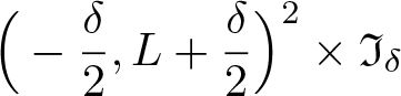 $\displaystyle\Big(-{\delta\over 2},L+{\delta\over 2}\Big)^2\times {\mathfrak{I}}_\delta$, (using (7.28) and (7.29)–(7.30))
 \begin{equation}
\begin{aligned}
(\textbf{I}_3+\nabla U_{e,{\varepsilon\delta}}-\textbf{R}_{\varepsilon\delta}^{\diamond})\textbf{e}_2&=0,\quad (\textbf{I}_3+\nabla U_{e,{\varepsilon\delta}}-\textbf{R}_{\varepsilon\delta}^{\diamond})\textbf{e}_3=0,\\
(\textbf{I}_3+\nabla U_{e,{\varepsilon\delta}}-\textbf{R}_{\varepsilon\delta}^{\diamond})\textbf{e}_1&=d_1{\mathcal{W}}_{\varepsilon\delta} +d_1\textbf{R}^{\diamond}_{\varepsilon\delta} x_3\textbf{e}_3.
\end{aligned}
\end{equation}
\begin{equation}
\begin{aligned}
(\textbf{I}_3+\nabla U_{e,{\varepsilon\delta}}-\textbf{R}_{\varepsilon\delta}^{\diamond})\textbf{e}_2&=0,\quad (\textbf{I}_3+\nabla U_{e,{\varepsilon\delta}}-\textbf{R}_{\varepsilon\delta}^{\diamond})\textbf{e}_3=0,\\
(\textbf{I}_3+\nabla U_{e,{\varepsilon\delta}}-\textbf{R}_{\varepsilon\delta}^{\diamond})\textbf{e}_1&=d_1{\mathcal{W}}_{\varepsilon\delta} +d_1\textbf{R}^{\diamond}_{\varepsilon\delta} x_3\textbf{e}_3.
\end{aligned}
\end{equation}Then, using (5.1), (7.35), and (7.36), we obtain
 \begin{equation*}
{1\over \varepsilon\sqrt{{\varepsilon\delta}}}\Pi_{\varepsilon\delta}^{(2)}\big((\nabla U_{e,{\varepsilon\delta}}-\textbf{R}_{\varepsilon\delta}^{\diamond}+\textbf{I}_3)\big)\textbf{e}_1\to Z+{y_1}d_1\textbf{A}\textbf{e}_1+{y_3}d_1\textbf{A}\textbf{e}_3 \;\text{strongly in}\ L^2({\omega}\times {\mathcal{Y}}_2)^3.
\end{equation*}
\begin{equation*}
{1\over \varepsilon\sqrt{{\varepsilon\delta}}}\Pi_{\varepsilon\delta}^{(2)}\big((\nabla U_{e,{\varepsilon\delta}}-\textbf{R}_{\varepsilon\delta}^{\diamond}+\textbf{I}_3)\big)\textbf{e}_1\to Z+{y_1}d_1\textbf{A}\textbf{e}_1+{y_3}d_1\textbf{A}\textbf{e}_3 \;\text{strongly in}\ L^2({\omega}\times {\mathcal{Y}}_2)^3.
\end{equation*}Using identities (7.37)–(7.38) and the above convergence and (7.32) yield the following strong convergence:
 \begin{equation}
{1\over 2\varepsilon\sqrt{{\varepsilon\delta}}}\Pi_{\varepsilon\delta}^{(2)}\big(((\nabla w_{\varepsilon\delta})^T(\nabla w_{\varepsilon\delta})-\textbf{I}_3)\big) \to E({\mathcal{W}}_{3},\widehat w)\quad \text{strongly in}\ L^2({\omega}\times {\mathcal{Y}}_2)^{3\times 3}
\end{equation}
\begin{equation}
{1\over 2\varepsilon\sqrt{{\varepsilon\delta}}}\Pi_{\varepsilon\delta}^{(2)}\big(((\nabla w_{\varepsilon\delta})^T(\nabla w_{\varepsilon\delta})-\textbf{I}_3)\big) \to E({\mathcal{W}}_{3},\widehat w)\quad \text{strongly in}\ L^2({\omega}\times {\mathcal{Y}}_2)^{3\times 3}
\end{equation}by proceeding as in Theorem 6.4.
Step 5. In this step, we provide the convergence of the right-hand side forces.
With definition of forces (4.60) and  $U_{e,{\varepsilon\delta}}$ (7.28), we get
 \begin{equation*}
\int_{\Omega_\delta}f_{\varepsilon\delta}\cdot U_{e,{\varepsilon\delta}}\,dx=\delta\int_{{\omega}_\delta} f_{\varepsilon\delta}\cdot {\mathcal{W}}_{{\varepsilon\delta}}\,dx'
+\delta\int_{{\omega}_\delta} f_{\varepsilon\delta}\cdot \big(\int_{-{\delta\over 2}}^{x_1}(\textbf{R}_{\varepsilon\delta}^{\diamond}-\textbf{I}_3)\textbf{e}_1\,dt\big)dx'
\end{equation*}
\begin{equation*}
\int_{\Omega_\delta}f_{\varepsilon\delta}\cdot U_{e,{\varepsilon\delta}}\,dx=\delta\int_{{\omega}_\delta} f_{\varepsilon\delta}\cdot {\mathcal{W}}_{{\varepsilon\delta}}\,dx'
+\delta\int_{{\omega}_\delta} f_{\varepsilon\delta}\cdot \big(\int_{-{\delta\over 2}}^{x_1}(\textbf{R}_{\varepsilon\delta}^{\diamond}-\textbf{I}_3)\textbf{e}_1\,dt\big)dx'
\end{equation*}and the scaling of  $\overline{w}_{\varepsilon\delta}$,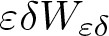 ${\varepsilon\delta} W_{\varepsilon\delta}$,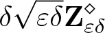 $\delta\sqrt{{\varepsilon\delta}}\textbf{Z}^{\diamond}_{\varepsilon\delta}$ give the following convergences of the forces with the convergences (7.32), (7.36) $_2$
$_2$
 \begin{equation}
\begin{aligned}
&\lim_{(\varepsilon,\delta)\to(0,0)}{1\over \varepsilon^2\delta^2}\big(\int_{{\omega}_\delta} f_{\varepsilon\delta}\cdot{\mathcal{W}}_{\varepsilon\delta}\,dx'\big)=0=
\lim_{(\varepsilon,\delta)\to(0,0)}{1\over \varepsilon^2\delta^3}\big(\int_{{\omega}_\delta} f_{\varepsilon\delta}\cdot\overline{w}_{\varepsilon\delta}\,dx'\big),\\
&\lim_{(\varepsilon,\delta)\to(0,0)}{1\over \varepsilon^2\delta^2}\int_{{\omega}_\delta} f_{1,{\varepsilon\delta}} \big(\int_{-{\delta\over 2}}^{x_1}(\textbf{R}_{\varepsilon\delta}^{\diamond}-\textbf{I}_3)\textbf{e}_1\cdot\textbf{e}_1\,dt\big)\,dx' =\int_{\omega} f_1{\mathcal{W}}_1\,dx',\\
&\lim_{(\varepsilon,\delta)\to(0,0)}{1\over \varepsilon^2\delta^2}\int_{{\omega}_\delta}f_{3,{\varepsilon\delta}} \big(\int_{-{\delta\over 2}}^{x_1}(\textbf{R}_{\varepsilon\delta}^{\diamond}-\textbf{I}_3)\textbf{e}_1\cdot\textbf{e}_3\,dt\big)\,dx'=\int_{\omega} f_3{\mathcal{W}}_3\,dx'.
\end{aligned}
\end{equation}
\begin{equation}
\begin{aligned}
&\lim_{(\varepsilon,\delta)\to(0,0)}{1\over \varepsilon^2\delta^2}\big(\int_{{\omega}_\delta} f_{\varepsilon\delta}\cdot{\mathcal{W}}_{\varepsilon\delta}\,dx'\big)=0=
\lim_{(\varepsilon,\delta)\to(0,0)}{1\over \varepsilon^2\delta^3}\big(\int_{{\omega}_\delta} f_{\varepsilon\delta}\cdot\overline{w}_{\varepsilon\delta}\,dx'\big),\\
&\lim_{(\varepsilon,\delta)\to(0,0)}{1\over \varepsilon^2\delta^2}\int_{{\omega}_\delta} f_{1,{\varepsilon\delta}} \big(\int_{-{\delta\over 2}}^{x_1}(\textbf{R}_{\varepsilon\delta}^{\diamond}-\textbf{I}_3)\textbf{e}_1\cdot\textbf{e}_1\,dt\big)\,dx' =\int_{\omega} f_1{\mathcal{W}}_1\,dx',\\
&\lim_{(\varepsilon,\delta)\to(0,0)}{1\over \varepsilon^2\delta^2}\int_{{\omega}_\delta}f_{3,{\varepsilon\delta}} \big(\int_{-{\delta\over 2}}^{x_1}(\textbf{R}_{\varepsilon\delta}^{\diamond}-\textbf{I}_3)\textbf{e}_1\cdot\textbf{e}_3\,dt\big)\,dx'=\int_{\omega} f_3{\mathcal{W}}_3\,dx'.
\end{aligned}
\end{equation}Step 6. We present the main result of the theorem.
From expressions (7.28), along with the estimates (7.33) and the definitions of the field  ${\mathcal{W}}_{\varepsilon\delta}$ and $\textbf{R}_{\varepsilon\delta}^\diamond$, we have
 \begin{equation*}\begin{aligned}
&\|\nabla w_{\varepsilon\delta}-\textbf{R}^\diamond_{\varepsilon\delta}\|_{L^\infty(\Omega_\delta)}\leq C\varepsilon\sqrt{{\varepsilon\delta}}.
\end{aligned}
\end{equation*}
\begin{equation*}\begin{aligned}
&\|\nabla w_{\varepsilon\delta}-\textbf{R}^\diamond_{\varepsilon\delta}\|_{L^\infty(\Omega_\delta)}\leq C\varepsilon\sqrt{{\varepsilon\delta}}.
\end{aligned}
\end{equation*}The above estimate give
 \begin{equation*}
\|\nabla w_{\varepsilon\delta}-\textbf{I}_3\|_{L^\infty(\Omega_\delta)}\leq \|\nabla w_{{\varepsilon\delta}}-\textbf{R}_{\varepsilon\delta}^{\diamond}\|_{L^\infty(\Omega_\delta)}+C\|\textbf{R}_{\varepsilon\delta}^{\diamond}-\textbf{I}_3\|_{L^\infty(-{\delta\over 2},L+{\delta\over2})}\leq C\sqrt{{\varepsilon\delta}},
\end{equation*}
\begin{equation*}
\|\nabla w_{\varepsilon\delta}-\textbf{I}_3\|_{L^\infty(\Omega_\delta)}\leq \|\nabla w_{{\varepsilon\delta}}-\textbf{R}_{\varepsilon\delta}^{\diamond}\|_{L^\infty(\Omega_\delta)}+C\|\textbf{R}_{\varepsilon\delta}^{\diamond}-\textbf{I}_3\|_{L^\infty(-{\delta\over 2},L+{\delta\over2})}\leq C\sqrt{{\varepsilon\delta}},
\end{equation*}where the constant  $C$ does not depend on $\varepsilon$ and $\delta$. Then, we obtain for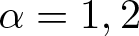 $\alpha=1,2$
 \begin{equation}
\begin{aligned}
\Pi_{\varepsilon\delta}^{(\alpha)}(\nabla w_{\varepsilon\delta})\to \textbf{I}_3,\quad \text{strongly in}\ L^\infty({\omega}\times {\mathcal{Y}}_\alpha)^{3\times 3},\\
\text{and}\quad \mathrm{det}(\nabla w_{\varepsilon\delta}) \gt 0,\quad\text{a.e. in}\ \Omega_\delta.
\end{aligned}
\end{equation}
\begin{equation}
\begin{aligned}
\Pi_{\varepsilon\delta}^{(\alpha)}(\nabla w_{\varepsilon\delta})\to \textbf{I}_3,\quad \text{strongly in}\ L^\infty({\omega}\times {\mathcal{Y}}_\alpha)^{3\times 3},\\
\text{and}\quad \mathrm{det}(\nabla w_{\varepsilon\delta}) \gt 0,\quad\text{a.e. in}\ \Omega_\delta.
\end{aligned}
\end{equation} So, the test function sequence  $\{w_{\varepsilon\delta}\}_{\varepsilon,\delta}\subset \textbf{V}_{\varepsilon\delta}$ satisfies $\textbf{W}_{\varepsilon\delta}(x,\nabla w_{\varepsilon\delta})=\textbf{Q}_{\varepsilon\delta}(x,\textbf{E}(\nabla w_{\varepsilon\delta}))$.
Due to (7.41) and  $\textbf{m}_{\varepsilon\delta}\leq \textbf{J}_{\varepsilon\delta}(w_{\varepsilon\delta})$, we have after passing $(\varepsilon,\delta)\to(0,0)$,
 \begin{align*}\limsup_{(\varepsilon,\delta)\to(0,0)}{\textbf{m}_{\varepsilon\delta}\over \varepsilon^2\delta^3} &\leq \lim_{(\varepsilon,\delta)\to(0,0)}{\textbf{J}_{\varepsilon\delta}(w_{\varepsilon\delta})\over \varepsilon^2\delta^3}=\textbf{W}\big({\mathcal{W}}_{3},0,\widehat {w}\big)\\
&\quad -\int_{{\omega}} f\cdot{\mathcal{W}}\,dx'= \textbf{J}({\mathcal{W}}_3,0,\widehat {w})=\textbf{J}^{(2)}({\mathcal{W}}_3,\widehat w).\end{align*}
\begin{align*}\limsup_{(\varepsilon,\delta)\to(0,0)}{\textbf{m}_{\varepsilon\delta}\over \varepsilon^2\delta^3} &\leq \lim_{(\varepsilon,\delta)\to(0,0)}{\textbf{J}_{\varepsilon\delta}(w_{\varepsilon\delta})\over \varepsilon^2\delta^3}=\textbf{W}\big({\mathcal{W}}_{3},0,\widehat {w}\big)\\
&\quad -\int_{{\omega}} f\cdot{\mathcal{W}}\,dx'= \textbf{J}({\mathcal{W}}_3,0,\widehat {w})=\textbf{J}^{(2)}({\mathcal{W}}_3,\widehat w).\end{align*} Since  ${\mathbb{D}}^{(2)}\cap\big( \mathcal{C}^2([0,L]_{x_1})\times \mathcal{C}^1([0,L]_{x_1}\times \overline{{\mathcal{Y}}_2})^3\big)$ is dense in ${\mathbb{D}}^{(2)}$ and $({\mathcal{W}}_3,\widehat w)\in {\mathbb{D}}^{(2)}\cap\big( \mathcal{C}^2([0,L]_{x_1})\times \mathcal{C}^1([0,L]_{x_1}\times \overline{{\mathcal{Y}}_2})^3\big)$ is arbitrary, we get
 \begin{equation*}
\limsup_{(\varepsilon,\delta)\to(0,0)}{\textbf{m}_{\varepsilon\delta}\over \varepsilon^2\delta^3}\leq\textbf{J}^{(2)}({\mathcal{W}}_3,\widehat w),\quad \forall\,({\mathcal{W}}_3,\widehat w)\in{\mathbb{D}}^{(2)}.
\end{equation*}
\begin{equation*}
\limsup_{(\varepsilon,\delta)\to(0,0)}{\textbf{m}_{\varepsilon\delta}\over \varepsilon^2\delta^3}\leq\textbf{J}^{(2)}({\mathcal{W}}_3,\widehat w),\quad \forall\,({\mathcal{W}}_3,\widehat w)\in{\mathbb{D}}^{(2)}.
\end{equation*} Finally, using the pair  $({\mathcal{W}}_3,\widehat w)\in {\mathbb{D}}^{(2)}$ which minimizes the functional $\textbf{J}^{(2)}$ over ${\mathbb{D}}^{(2)}$, we obtain
 \begin{equation*}\limsup_{(\varepsilon,\delta)\to(0,0)}{\textbf{m}_{\varepsilon\delta}\over \varepsilon^2\delta^3}\leq\textbf{m}^{(2)}.\end{equation*}
This completes the proof.
Finally, we have the main convergence result of this paper
Theorem 7.7. With assumption on forces (4.60)–(4.61) and the Hooke’s coefficient 7.3, we have
 \begin{equation}
\lim_{(\varepsilon,\delta)\to(0,0)}{\textbf{m}_{\varepsilon\delta}\over \varepsilon^2\delta^3}= \textbf{m}.
\end{equation}
\begin{equation}
\lim_{(\varepsilon,\delta)\to(0,0)}{\textbf{m}_{\varepsilon\delta}\over \varepsilon^2\delta^3}= \textbf{m}.
\end{equation}Proof. This theorem is an immediate consequence of Propositions 7.1, 7.4, 7.5, and 7.6.
Appendix A.
In the appendix, we give the proof of the preliminary estimates for existence of minimizer of the limit unfolded energy.
Proof of Lemma 7.2
Step 1. We show that
 \begin{equation}
\begin{aligned}
&\|\overline{v}_1\|_{L^2({\mathcal{Y}}_1)}+|\textbf{a}_1|+|\textbf{b}_1|+|{\mathcal{G}}_1|
\leq C\Big(\|\partial_{y_2}\widehat v_1\|_{L^2({\mathcal{Y}}_1)}+\|\partial_{y_3}\widehat v_1\|_{L^2({\mathcal{Y}}_1)}\big),\\
&\|\partial_{y_2}\overline{v}_1\|_{L^2({\mathcal{Y}}_1)}+\|\partial_{y_3}\overline{v}_1\|_{L^2({\mathcal{Y}}_1)} \leq C\Big(\|\partial_{y_2}\widehat v_1\|_{L^2({\mathcal{Y}}_1)}+\|\partial_{y_3}\widehat v_1\|_{L^2({\mathcal{Y}}_1)}\big).
\end{aligned}
\end{equation}
\begin{equation}
\begin{aligned}
&\|\overline{v}_1\|_{L^2({\mathcal{Y}}_1)}+|\textbf{a}_1|+|\textbf{b}_1|+|{\mathcal{G}}_1|
\leq C\Big(\|\partial_{y_2}\widehat v_1\|_{L^2({\mathcal{Y}}_1)}+\|\partial_{y_3}\widehat v_1\|_{L^2({\mathcal{Y}}_1)}\big),\\
&\|\partial_{y_2}\overline{v}_1\|_{L^2({\mathcal{Y}}_1)}+\|\partial_{y_3}\overline{v}_1\|_{L^2({\mathcal{Y}}_1)} \leq C\Big(\|\partial_{y_2}\widehat v_1\|_{L^2({\mathcal{Y}}_1)}+\|\partial_{y_3}\widehat v_1\|_{L^2({\mathcal{Y}}_1)}\big).
\end{aligned}
\end{equation} We first apply the Poincaré–Wirtinger inequality to the cross sections 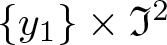 $\{y_1\}\times {\mathfrak{I}}^2$ with the function $\widehat v_1$. So, there exists $A_1\in L^2(0,1)$ such that
 \begin{equation}
\|\widehat v_1-A_1\|_{L^2((0,1) ; H^1({\mathfrak{I}}^2))} \leq C\big(\|\partial_{y_2}\widehat {v}_1\|_{L^2({\mathcal{Y}}_1)}+\|\partial_{y_3}\widehat {v}_1\|_{L^2({\mathcal{Y}}_1)}\big).
\end{equation}
\begin{equation}
\|\widehat v_1-A_1\|_{L^2((0,1) ; H^1({\mathfrak{I}}^2))} \leq C\big(\|\partial_{y_2}\widehat {v}_1\|_{L^2({\mathcal{Y}}_1)}+\|\partial_{y_3}\widehat {v}_1\|_{L^2({\mathcal{Y}}_1)}\big).
\end{equation}This implies the following estimates for the traces:
 \begin{equation*}
\|\widehat v_1(\cdot,-{1\over 2},\cdot)-A_1\|_{L^2((0,1)\times {\mathfrak{I}})}+\|\widehat v_1(\cdot,{1\over 2},\cdot)-A_1\|_{L^2((0,1)\times {\mathfrak{I}})} \leq C\|\widehat v_1-A_1\|_{L^2((0,1) ; H^1({\mathfrak{I}}^2))}.
\end{equation*}
\begin{equation*}
\|\widehat v_1(\cdot,-{1\over 2},\cdot)-A_1\|_{L^2((0,1)\times {\mathfrak{I}})}+\|\widehat v_1(\cdot,{1\over 2},\cdot)-A_1\|_{L^2((0,1)\times {\mathfrak{I}})} \leq C\|\widehat v_1-A_1\|_{L^2((0,1) ; H^1({\mathfrak{I}}^2))}.
\end{equation*} So (note that  $\textbf{a}_i=\textbf{a}\cdot\textbf{e}_i$, $\ldots\ldots$,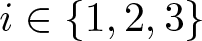 $i\in\{1,2,3\}$)
 \begin{equation*}\begin{aligned}
\|(\textbf{a}_1+\textbf{b}_1 y_1+{\mathcal{G}}_1y_3)+A_1\|_{L^2((0,1)\times {\mathfrak{I}})}+\|(\textbf{a}_1+\textbf{b}_1y_1+{\mathcal{G}}_1y_3)-A_1\|_{L^2((0,1)\times {\mathfrak{I}})}\\
\leq C\big(\|\partial_{y_2}\widehat {v}_1\|_{L^2({\mathcal{Y}}_1)}+\|\partial_{y_3}\widehat {v}_1\|_{L^2({\mathcal{Y}}_1)}\big),
\end{aligned}
\end{equation*}
\begin{equation*}\begin{aligned}
\|(\textbf{a}_1+\textbf{b}_1 y_1+{\mathcal{G}}_1y_3)+A_1\|_{L^2((0,1)\times {\mathfrak{I}})}+\|(\textbf{a}_1+\textbf{b}_1y_1+{\mathcal{G}}_1y_3)-A_1\|_{L^2((0,1)\times {\mathfrak{I}})}\\
\leq C\big(\|\partial_{y_2}\widehat {v}_1\|_{L^2({\mathcal{Y}}_1)}+\|\partial_{y_3}\widehat {v}_1\|_{L^2({\mathcal{Y}}_1)}\big),
\end{aligned}
\end{equation*}which first implies
 \begin{equation} \|\textbf{a}_1+\textbf{b}_1 y_1+{\mathcal{G}}_1y_3\|_{L^2((0,1)\times {\mathfrak{I}})}+\|A_1\|_{L^2((0,1)\times {\mathfrak{I}})}
\leq C\big(\|\partial_{y_2}\widehat {v}_1\|_{L^2({\mathcal{Y}}_1)}+\|\partial_{y_3}\widehat {v}_1\|_{L^2({\mathcal{Y}}_1)}\big),
\end{equation}
\begin{equation} \|\textbf{a}_1+\textbf{b}_1 y_1+{\mathcal{G}}_1y_3\|_{L^2((0,1)\times {\mathfrak{I}})}+\|A_1\|_{L^2((0,1)\times {\mathfrak{I}})}
\leq C\big(\|\partial_{y_2}\widehat {v}_1\|_{L^2({\mathcal{Y}}_1)}+\|\partial_{y_3}\widehat {v}_1\|_{L^2({\mathcal{Y}}_1)}\big),
\end{equation}then, as a consequence
 \begin{equation}
\begin{aligned}
|\textbf{a}_1|+|\textbf{b}_1|+|{\mathcal{G}}_1|+ \|A_1\|_{L^2((0,1)\times {\mathfrak{I}})}\leq C\big(\|\partial_{y_2}\widehat {v}_1\|_{L^2({\mathcal{Y}}_1)}+\|\partial_{y_3}\widehat {v}_1\|_{L^2({\mathcal{Y}}_1)}\big).
\end{aligned}
\end{equation}
\begin{equation}
\begin{aligned}
|\textbf{a}_1|+|\textbf{b}_1|+|{\mathcal{G}}_1|+ \|A_1\|_{L^2((0,1)\times {\mathfrak{I}})}\leq C\big(\|\partial_{y_2}\widehat {v}_1\|_{L^2({\mathcal{Y}}_1)}+\|\partial_{y_3}\widehat {v}_1\|_{L^2({\mathcal{Y}}_1)}\big).
\end{aligned}
\end{equation} As a consequence of the above and (A.2) we obtain (A.1) $_1$.
$_1$.
From the definition of  $\widehat v_1$, we have that $\overline{v}_1$ satisfies a Dirichlet boundary condition, so we use Green’s first identity and change of variable to obtain
 \begin{equation*}\begin{aligned}
\|\partial_{y_3}\overline{v}_1\|^2_{L^2({\mathcal{Y}}_1)}&\leq \|\partial_{y_3}\widehat v_1\|^2_{L^2({\mathcal{Y}}_1)}+{4\over 3}|{\mathcal{G}}_1|^2,\\ \|\partial_{y_2}\overline{v}_1\|^2_{L^2({\mathcal{Y}}_1)}&\leq \|\partial_{y_2}\widehat v_1\|^2_{L^2({\mathcal{Y}}_1)}+2\|\textbf{a}_1+\textbf{b}_1 y_1+{\mathcal{G}}_1y_3\|^2_{L^2((0,1)\times {\mathfrak{I}})},
\end{aligned}
\end{equation*}
\begin{equation*}\begin{aligned}
\|\partial_{y_3}\overline{v}_1\|^2_{L^2({\mathcal{Y}}_1)}&\leq \|\partial_{y_3}\widehat v_1\|^2_{L^2({\mathcal{Y}}_1)}+{4\over 3}|{\mathcal{G}}_1|^2,\\ \|\partial_{y_2}\overline{v}_1\|^2_{L^2({\mathcal{Y}}_1)}&\leq \|\partial_{y_2}\widehat v_1\|^2_{L^2({\mathcal{Y}}_1)}+2\|\textbf{a}_1+\textbf{b}_1 y_1+{\mathcal{G}}_1y_3\|^2_{L^2((0,1)\times {\mathfrak{I}})},
\end{aligned}
\end{equation*}which along with (A.3)–(A.4) give (A.1) $_2$.
$_2$.
Step 2. We show that
 \begin{equation}
\begin{aligned}
&\|\overline{v}_i\|_{L^2({\mathcal{Y}}_1)}+\|\partial_{y_2}\overline{v}_i\|_{L^2({\mathcal{Y}}_1)}+\|\partial_{y_3}\overline{v}_i\|_{L^2({\mathcal{Y}}_1)}+|\textbf{a}_i|+|\textbf{b}_i|+|{\mathcal{G}}_i|\\
&\leq C\Big(\|e_{22,y}(\widehat v)\|_{L^2({\mathcal{Y}}_1)}+\|e_{23,y}(\widehat v)\|_{L^2({\mathcal{Y}}_1)}+\|e_{33,y}(\widehat v)\|_{L^2({\mathcal{Y}}_1)}\big),\qquad i\in\{2,3\}.
\end{aligned}
\end{equation}
\begin{equation}
\begin{aligned}
&\|\overline{v}_i\|_{L^2({\mathcal{Y}}_1)}+\|\partial_{y_2}\overline{v}_i\|_{L^2({\mathcal{Y}}_1)}+\|\partial_{y_3}\overline{v}_i\|_{L^2({\mathcal{Y}}_1)}+|\textbf{a}_i|+|\textbf{b}_i|+|{\mathcal{G}}_i|\\
&\leq C\Big(\|e_{22,y}(\widehat v)\|_{L^2({\mathcal{Y}}_1)}+\|e_{23,y}(\widehat v)\|_{L^2({\mathcal{Y}}_1)}+\|e_{33,y}(\widehat v)\|_{L^2({\mathcal{Y}}_1)}\big),\qquad i\in\{2,3\}.
\end{aligned}
\end{equation} The  $2$D-Korn’s inequality applied to the cross sections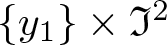 $\{y_1\}\times {\mathfrak{I}}^2$ gives $A_2,\; A_3,\; B\in L^2(0,1)$ such that
 \begin{equation}
\|\widehat {V}-R\|_{L^2((0,1); H^1({\mathfrak{I}}^2))}\leq C\big(\|e_{22,y}(\widehat v)\|_{L^2({\mathcal{Y}}_1)}+\|e_{23,y}(\widehat v)\|_{L^2({\mathcal{Y}}_1)}+\|e_{33,y}(\widehat v)\|_{L^2({\mathcal{Y}}_1)}\big)
\end{equation}
\begin{equation}
\|\widehat {V}-R\|_{L^2((0,1); H^1({\mathfrak{I}}^2))}\leq C\big(\|e_{22,y}(\widehat v)\|_{L^2({\mathcal{Y}}_1)}+\|e_{23,y}(\widehat v)\|_{L^2({\mathcal{Y}}_1)}+\|e_{33,y}(\widehat v)\|_{L^2({\mathcal{Y}}_1)}\big)
\end{equation}where  $\widehat {V}=\widehat {v}_2\textbf{e}_2+\widehat {v}_3\textbf{e}_3$ and $R$ is the $2D$ rigid displacement
 \begin{equation*}
R(y)=\big(A_2(y_1)-B(y_1)y_3\big)\textbf{e}_2+\big(A_3(y_1)+B(y_1)y_2\big)\textbf{e}_3\qquad \hbox{for a.e. } y\in {\mathcal{Y}}^{(1)}.
\end{equation*}
\begin{equation*}
R(y)=\big(A_2(y_1)-B(y_1)y_3\big)\textbf{e}_2+\big(A_3(y_1)+B(y_1)y_2\big)\textbf{e}_3\qquad \hbox{for a.e. } y\in {\mathcal{Y}}^{(1)}.
\end{equation*}This implies the following estimates for the traces:
 \begin{equation*}
\begin{aligned}
&\|\widehat V_2(\cdot,-{1\over 2},\cdot)-A_2+B y_3\|_{L^2((0,1)\times {\mathfrak{I}})}+\|\widehat V_2(\cdot,{1\over 2},\cdot)-A_2+B y_3\|_{L^2((0,1)\times {\mathfrak{I}})}\\
\leq &C\|\widehat V_2-R_2\|_{L^2((0,1) ; H^1({\mathfrak{I}}^2))}\leq C\big(\|e_{22,y}(\widehat v)\|_{L^2({\mathcal{Y}}_1)}+\|e_{23,y}(\widehat v)\|_{L^2({\mathcal{Y}}_1)}\\
&+\|e_{33,y}(\widehat v)\|_{L^2({\mathcal{Y}}_1)}\big).
\end{aligned}
\end{equation*}
\begin{equation*}
\begin{aligned}
&\|\widehat V_2(\cdot,-{1\over 2},\cdot)-A_2+B y_3\|_{L^2((0,1)\times {\mathfrak{I}})}+\|\widehat V_2(\cdot,{1\over 2},\cdot)-A_2+B y_3\|_{L^2((0,1)\times {\mathfrak{I}})}\\
\leq &C\|\widehat V_2-R_2\|_{L^2((0,1) ; H^1({\mathfrak{I}}^2))}\leq C\big(\|e_{22,y}(\widehat v)\|_{L^2({\mathcal{Y}}_1)}+\|e_{23,y}(\widehat v)\|_{L^2({\mathcal{Y}}_1)}\\
&+\|e_{33,y}(\widehat v)\|_{L^2({\mathcal{Y}}_1)}\big).
\end{aligned}
\end{equation*} Then, using the fact that  $\overline{v}_2(\cdot,\pm {1\over 2},\cdot)=0$, as in Step 1 we obtain
 \begin{equation*}\begin{aligned}
\|\textbf{a}_2+\textbf{b}_2y_1+{\mathcal{G}}_2y_3\|_{L^2((0,1)\times {\mathfrak{I}})}+\|A_2-y_3 B\|_{L^2((0,1)\times {\mathfrak{I}})}\\
\leq C\big(\|e_{22,y}(\widehat v)\|_{L^2({\mathcal{Y}}_1)}+\|e_{23,y}(\widehat v)\|_{L^2({\mathcal{Y}}_1)}+\|e_{33,y}(\widehat v)\|_{L^2({\mathcal{Y}}_1)}\big),
\end{aligned}
\end{equation*}
\begin{equation*}\begin{aligned}
\|\textbf{a}_2+\textbf{b}_2y_1+{\mathcal{G}}_2y_3\|_{L^2((0,1)\times {\mathfrak{I}})}+\|A_2-y_3 B\|_{L^2((0,1)\times {\mathfrak{I}})}\\
\leq C\big(\|e_{22,y}(\widehat v)\|_{L^2({\mathcal{Y}}_1)}+\|e_{23,y}(\widehat v)\|_{L^2({\mathcal{Y}}_1)}+\|e_{33,y}(\widehat v)\|_{L^2({\mathcal{Y}}_1)}\big),
\end{aligned}
\end{equation*}which gives
 \begin{equation}\begin{aligned}
\|A_2\|_{L^2(0,1)}+\|B\|_{L^2(0,1)}+|\textbf{a}_2|+|\textbf{b}_2|+|{\mathcal{G}}_2|\\
\leq C\big(\|e_{22,y}(\widehat v)\|_{L^2({\mathcal{Y}}_1)}+\|e_{23,y}(\widehat v)\|_{L^2({\mathcal{Y}}_1)}+\|e_{33,y}(\widehat v)\|_{L^2({\mathcal{Y}}_1)}\big).
\end{aligned}
\end{equation}
\begin{equation}\begin{aligned}
\|A_2\|_{L^2(0,1)}+\|B\|_{L^2(0,1)}+|\textbf{a}_2|+|\textbf{b}_2|+|{\mathcal{G}}_2|\\
\leq C\big(\|e_{22,y}(\widehat v)\|_{L^2({\mathcal{Y}}_1)}+\|e_{23,y}(\widehat v)\|_{L^2({\mathcal{Y}}_1)}+\|e_{33,y}(\widehat v)\|_{L^2({\mathcal{Y}}_1)}\big).
\end{aligned}
\end{equation} For the component in the  $\textbf{e}_3$ direction, we first obtain using (A.6)
 \begin{equation*}
\begin{aligned}
&\|\widehat V_3(\cdot,-{1\over 2},\cdot)-A_3+B y_2 \|_{L^2((0,1)\times {\mathfrak{I}})}+\|\widehat V_2(\cdot,{1\over 2},\cdot)-A_3-B y_2\|_{L^2((0,1)\times {\mathfrak{I}})}\\
\leq &C\|\widehat V_3-R_3\|_{L^2((0,1) ; H^1({\mathfrak{I}}^2))}\leq C\big(\|e_{22,y}(\widehat v)\|_{L^2({\mathcal{Y}}_1)}\\
&\quad +\|e_{23,y}(\widehat v)\|_{L^2({\mathcal{Y}}_1)}+\|e_{33,y}(\widehat v)\|_{L^2({\mathcal{Y}}_1)}\big).
\end{aligned}
\end{equation*}
\begin{equation*}
\begin{aligned}
&\|\widehat V_3(\cdot,-{1\over 2},\cdot)-A_3+B y_2 \|_{L^2((0,1)\times {\mathfrak{I}})}+\|\widehat V_2(\cdot,{1\over 2},\cdot)-A_3-B y_2\|_{L^2((0,1)\times {\mathfrak{I}})}\\
\leq &C\|\widehat V_3-R_3\|_{L^2((0,1) ; H^1({\mathfrak{I}}^2))}\leq C\big(\|e_{22,y}(\widehat v)\|_{L^2({\mathcal{Y}}_1)}\\
&\quad +\|e_{23,y}(\widehat v)\|_{L^2({\mathcal{Y}}_1)}+\|e_{33,y}(\widehat v)\|_{L^2({\mathcal{Y}}_1)}\big).
\end{aligned}
\end{equation*} Taking into account the estimate (A.7) $_2$ of $B$, this leads to
 \begin{equation*}\begin{aligned}
\|\textbf{a}_3+\textbf{b}_3y_1+{\mathcal{G}}_3 y_3+A_3\|_{L^2((0,1)\times {\mathfrak{I}})}+ \|\textbf{a}_3+\textbf{b}_3y_1+{\mathcal{G}}_3 y_3-A_3\|_{L^2((0,1)\times {\mathfrak{I}})}\\
\leq C\big(\|e_{22,y}(\widehat v)\|_{L^2({\mathcal{Y}}_1)}+\|e_{23,y}(\widehat v)\|_{L^2({\mathcal{Y}}_1)}+\|e_{33,y}(\widehat v)\|_{L^2({\mathcal{Y}}_1)}\big),
\end{aligned}
\end{equation*}
\begin{equation*}\begin{aligned}
\|\textbf{a}_3+\textbf{b}_3y_1+{\mathcal{G}}_3 y_3+A_3\|_{L^2((0,1)\times {\mathfrak{I}})}+ \|\textbf{a}_3+\textbf{b}_3y_1+{\mathcal{G}}_3 y_3-A_3\|_{L^2((0,1)\times {\mathfrak{I}})}\\
\leq C\big(\|e_{22,y}(\widehat v)\|_{L^2({\mathcal{Y}}_1)}+\|e_{23,y}(\widehat v)\|_{L^2({\mathcal{Y}}_1)}+\|e_{33,y}(\widehat v)\|_{L^2({\mathcal{Y}}_1)}\big),
\end{aligned}
\end{equation*}which give
 \begin{align*}
&|\textbf{a}_3|+|\textbf{b}_3|+|{\mathcal{G}}_3|+ \|A_3\|_{L^2((0,1)\times {\mathfrak{I}})}\\
&\leq C\big(\|e_{22,y}(\widehat v)\|_{L^2({\mathcal{Y}}_1)}+\|e_{23,y}(\widehat v)\|_{L^2({\mathcal{Y}}_1)}+\|e_{33,y}(\widehat v)\|_{L^2({\mathcal{Y}}_1)}\big).\end{align*}
\begin{align*}
&|\textbf{a}_3|+|\textbf{b}_3|+|{\mathcal{G}}_3|+ \|A_3\|_{L^2((0,1)\times {\mathfrak{I}})}\\
&\leq C\big(\|e_{22,y}(\widehat v)\|_{L^2({\mathcal{Y}}_1)}+\|e_{23,y}(\widehat v)\|_{L^2({\mathcal{Y}}_1)}+\|e_{33,y}(\widehat v)\|_{L^2({\mathcal{Y}}_1)}\big).\end{align*} The above inequality with (A.6), (A.7), and definition of  $\widehat v_i$ (with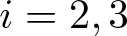 $i=2,3$) gives (A.5). This completes the proof.
As a consequence, we have
Proof of Lemma 7.3
Observe that  $\widehat v^{(1)}=\overline{v}^{(1)}+y_2Z^{(1)}+y_1y_2{\mathcal{Z}}$, where $\overline{v}^{(1)}\in L^2({\omega}\times (0,1)_{y_1};H^1({\mathfrak{I}}^2))^3$ with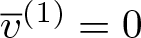 $\overline{v}^{(1)}=0$ satisfying (6.19) $_1$ and $Z^{(1)},{\mathcal{Z}}\in L^2({\omega})^3$. Set
 \begin{equation}
\widehat w^{(1)}=\overline{v}^{(1)}+y_2Z^{(1)}+y_1y_2{\mathcal{Z}}-y_2y_3 d^2_{22}{\mathcal{U}}_3^{(1)}\textbf{e}_2\qquad \hbox{a.e. in }{\omega}\times {\mathcal{Y}}_1.
\end{equation}
\begin{equation}
\widehat w^{(1)}=\overline{v}^{(1)}+y_2Z^{(1)}+y_1y_2{\mathcal{Z}}-y_2y_3 d^2_{22}{\mathcal{U}}_3^{(1)}\textbf{e}_2\qquad \hbox{a.e. in }{\omega}\times {\mathcal{Y}}_1.
\end{equation} Then, Lemma 7.2 gives (7.14) $_1$. Similarly, we show (7.14) $_2$.
$_2$.