


1. Introduction
The development of aerospace technologies that travel with a flight Mach number ( $M_{\infty }$
) well above sonic is challenged by complex aerothermodynamic behaviours. This flight regime is typically referred to as hypersonic. Boundary layer instability and transition can significantly constrain the flight envelope and operation limits of hypersonic vehicles (Lin Reference Lin2008). The location point of laminar-to-turbulent transition in hypersonic boundary layers has a significant influence on viscous drag and aerodynamic heating of external surfaces of hypersonic vehicles, and is a dominant source of uncertainties during the design process (Shea Reference Shea1992). Relative to a laminar state, the heat flux for a turbulent boundary layer can be up to eight times greater (Leyva Reference Leyva2017). Thus, this motivates further research on transition control.
$M_{\infty }$
) well above sonic is challenged by complex aerothermodynamic behaviours. This flight regime is typically referred to as hypersonic. Boundary layer instability and transition can significantly constrain the flight envelope and operation limits of hypersonic vehicles (Lin Reference Lin2008). The location point of laminar-to-turbulent transition in hypersonic boundary layers has a significant influence on viscous drag and aerodynamic heating of external surfaces of hypersonic vehicles, and is a dominant source of uncertainties during the design process (Shea Reference Shea1992). Relative to a laminar state, the heat flux for a turbulent boundary layer can be up to eight times greater (Leyva Reference Leyva2017). Thus, this motivates further research on transition control.
For laminar hypersonic boundary layers, an important non-dimensional parameter is the relative Mach number $\overline {M}$
, which is defined based on the velocity of the flow (
$\overline {M}$
, which is defined based on the velocity of the flow ( $u$
) relative to the phase speed (
$u$
) relative to the phase speed ( $c_{ph}$
) of the hydrodynamic instability within the boundary layer. When
$c_{ph}$
) of the hydrodynamic instability within the boundary layer. When $\overline {M}^2\gt 1$
, the compressible counterpart of the Rayleigh’s equation admits multiple wave-like solutions, also referred to as higher Mack modes (Mack Reference Mack1969). For a flight Mach number (
$\overline {M}^2\gt 1$
, the compressible counterpart of the Rayleigh’s equation admits multiple wave-like solutions, also referred to as higher Mack modes (Mack Reference Mack1969). For a flight Mach number ( $M_{\infty }$
) approximately between 4 and 6, and for a thermally insulated (adiabatic) wall, or under thermal equilibrium conditions (radiative–adiabatic, Anderson Reference Anderson1989), an important boundary layer instability mechanism is known to be two-dimensional and dominated by high-frequency,
$M_{\infty }$
) approximately between 4 and 6, and for a thermally insulated (adiabatic) wall, or under thermal equilibrium conditions (radiative–adiabatic, Anderson Reference Anderson1989), an important boundary layer instability mechanism is known to be two-dimensional and dominated by high-frequency, $ \tilde {f} \in [10^5, 10^6]$
Hz (Laurence, Wagner & Hannemann Reference Laurence, Wagner and Hannemann2016), thermoacoustically driven (Kuehl Reference Kuehl2018) waves trapped between the wall and the relative sonic line within the boundary layer (Mack Reference Mack1975). This instability mechanism is typically referred to as the second Mack mode. Although this is not a mode in a mathematical sense (Fedorov & Tumin Reference Fedorov and Tumin2011), the terminology is still generally accepted in the literature and therefore it is also used within the context of this work. The high-frequency dilatation work of the second Mack mode instability on the flow can also lead to significant local aerodynamic heating (Zhu et al. Reference Zhu, Chen, Wu, Chen, Lee and Gad-el-Hak2018), which can further reduce the aerothermal efficiency of hypersonic vehicles.
$ \tilde {f} \in [10^5, 10^6]$
Hz (Laurence, Wagner & Hannemann Reference Laurence, Wagner and Hannemann2016), thermoacoustically driven (Kuehl Reference Kuehl2018) waves trapped between the wall and the relative sonic line within the boundary layer (Mack Reference Mack1975). This instability mechanism is typically referred to as the second Mack mode. Although this is not a mode in a mathematical sense (Fedorov & Tumin Reference Fedorov and Tumin2011), the terminology is still generally accepted in the literature and therefore it is also used within the context of this work. The high-frequency dilatation work of the second Mack mode instability on the flow can also lead to significant local aerodynamic heating (Zhu et al. Reference Zhu, Chen, Wu, Chen, Lee and Gad-el-Hak2018), which can further reduce the aerothermal efficiency of hypersonic vehicles.
The stability of compressible boundary layers is significantly affected by wall temperature (Lees & Lin Reference Lees and Lin1946). This is an important consideration for ground-testing. In high-enthalpy (flight representative) facilities, the wall temperature can be a small fraction of the free stream temperature ( $\tilde {T}_w/\tilde {T}_{\infty }\approx 0.1-0.3$
, Bitter & Shepherd Reference Bitter and Shepherd2015), while this is not usually the case in wind tunnels operated at lower stagnation enthalpies. Based on Rayleigh’s generalised inflection theorem (Rayleigh Reference Rayleigh1895), inviscid inflectional instability modes can be stabilised by sufficient wall cooling for low-speed and supersonic flows (Masad, Nayfeh & Al-Maaitah Reference Masad, Nayfeh and Al-Maaitah1992). However, this is no longer true when higher Mack modes arise in hypersonic boundary layers. In particular, the second Mack mode is destabilised by wall cooling (Mack Reference Mack1975; Bitter & Shepherd Reference Bitter and Shepherd2015). This effect is further exacerbated when the wall temperature is further reduced (
$\tilde {T}_w/\tilde {T}_{\infty }\approx 0.1-0.3$
, Bitter & Shepherd Reference Bitter and Shepherd2015), while this is not usually the case in wind tunnels operated at lower stagnation enthalpies. Based on Rayleigh’s generalised inflection theorem (Rayleigh Reference Rayleigh1895), inviscid inflectional instability modes can be stabilised by sufficient wall cooling for low-speed and supersonic flows (Masad, Nayfeh & Al-Maaitah Reference Masad, Nayfeh and Al-Maaitah1992). However, this is no longer true when higher Mack modes arise in hypersonic boundary layers. In particular, the second Mack mode is destabilised by wall cooling (Mack Reference Mack1975; Bitter & Shepherd Reference Bitter and Shepherd2015). This effect is further exacerbated when the wall temperature is further reduced ( $\tilde {T}_w/\tilde {T}_{\infty }\lt 0.1$
) and unstable supersonic modes also manifest (Bitter & Shepherd Reference Bitter and Shepherd2015; Chuvakhov & Fedorov Reference Chuvakhov and Fedorov2016; Saikia, Hasnine & Brehm Reference Saikia, Hasnine and Brehm2022). Wall heating instead tends to stabilise the second Mack mode (Mack Reference Mack1975). On the other hand, three-dimensional, inflectional instabilities (e.g. first Mack mode) are stabilised by wall cooling (Mack Reference Mack1969; Lysenko & Maslov Reference Lysenko and Maslov1984). As a result of the significant impact of wall temperature on first and second Mack modes, several transition control strategies that exploit surface heat flux have been numerically attempted in the literature (Zhao et al. Reference Zhao, Wen, Tian, Long and Yuan2018; Jahanbakhshi & Zaki Reference Jahanbakhshi and Zaki2021; Poulain Reference Poulain2023). Although effective, active flow control techniques require careful energy input considerations (Frohnapfel, Hasegawa & Quadrio Reference Frohnapfel, Hasegawa and Quadrio2012). In addition, the practical and robust implementation of active flow control devices remains a challenge (Gad-el Hak Reference Gad-el Hak2001).
$\tilde {T}_w/\tilde {T}_{\infty }\lt 0.1$
) and unstable supersonic modes also manifest (Bitter & Shepherd Reference Bitter and Shepherd2015; Chuvakhov & Fedorov Reference Chuvakhov and Fedorov2016; Saikia, Hasnine & Brehm Reference Saikia, Hasnine and Brehm2022). Wall heating instead tends to stabilise the second Mack mode (Mack Reference Mack1975). On the other hand, three-dimensional, inflectional instabilities (e.g. first Mack mode) are stabilised by wall cooling (Mack Reference Mack1969; Lysenko & Maslov Reference Lysenko and Maslov1984). As a result of the significant impact of wall temperature on first and second Mack modes, several transition control strategies that exploit surface heat flux have been numerically attempted in the literature (Zhao et al. Reference Zhao, Wen, Tian, Long and Yuan2018; Jahanbakhshi & Zaki Reference Jahanbakhshi and Zaki2021; Poulain Reference Poulain2023). Although effective, active flow control techniques require careful energy input considerations (Frohnapfel, Hasegawa & Quadrio Reference Frohnapfel, Hasegawa and Quadrio2012). In addition, the practical and robust implementation of active flow control devices remains a challenge (Gad-el Hak Reference Gad-el Hak2001).
Passive control of hypersonic boundary layer transition has been experimentally and numerically attempted through the use of roughness elements (Marxen, Iaccarino & Shaqfeh Reference Marxen, Iaccarino and Shaqfeh2010; Fong et al. Reference Fong, Wang, Huang, Zhong, McKiernan, Fisher and Schneider2015; Taylor & Bruce Reference Taylor and Bruce2016) or vortex generators (Paredes, Choudhari & Li Reference Paredes, Choudhari and Li2019). Marxen et al. (Reference Marxen, Iaccarino and Shaqfeh2010) used high-order compressible direct numerical simulation (DNS) computations to investigate the growth rate of convective disturbances within a boundary layer at $M_{\infty }=4.8$
with two-dimensional roughness elements. For high-frequency (second Mack mode type) disturbances, the spatial damping effect of the two-dimensional, localised, roughness elements was significant. For a similar geometry configuration and for
$M_{\infty }=4.8$
with two-dimensional roughness elements. For high-frequency (second Mack mode type) disturbances, the spatial damping effect of the two-dimensional, localised, roughness elements was significant. For a similar geometry configuration and for $M_{\infty }=5.92$
, Duan, Wang & Zhong (Reference Duan, Wang and Zhong2013) showed that the streamwise position of the roughness element is an important factor in the control of two- and three-dimensional (oblique) instabilities. For a cone configuration, Fong et al. (Reference Fong, Wang, Huang, Zhong, McKiernan, Fisher and Schneider2015) showed that if the streamwise locations of the roughness elements is informed by numerical (linear) analysis of the boundary layer stability, it is possible to achieve stabilisation of both first and second Mack modes. However, these passive control devices present several implementation challenges at hypersonic speeds due to their long exposure to high heat flux. Thus, novel robust control methods are required for hypersonic regimes.
$M_{\infty }=5.92$
, Duan, Wang & Zhong (Reference Duan, Wang and Zhong2013) showed that the streamwise position of the roughness element is an important factor in the control of two- and three-dimensional (oblique) instabilities. For a cone configuration, Fong et al. (Reference Fong, Wang, Huang, Zhong, McKiernan, Fisher and Schneider2015) showed that if the streamwise locations of the roughness elements is informed by numerical (linear) analysis of the boundary layer stability, it is possible to achieve stabilisation of both first and second Mack modes. However, these passive control devices present several implementation challenges at hypersonic speeds due to their long exposure to high heat flux. Thus, novel robust control methods are required for hypersonic regimes.
Effective transition delay for low-speed boundary layers using optimal streaks has been demonstrated by experimental (Fransson et al. Reference Fransson, Talamelli, Brandt and Cossu2006) and numerical (Cossu & Brandt Reference Cossu and Brandt2002; Schlatter et al. Reference Schlatter, Deusebio, de Lange and Brandt2010) studies. Bagheri & Hanifi (Reference Bagheri and Hanifi2007) showed that Tollmien–Schlichting waves and oblique waves can be stabilised by finite amplitude streaks, that modify the mean flow distortion. It was also shown that the streak wavenumber for optimal growth of the streaks is not the most efficient to achieve Tollmien–Schlichting-wave stabilisation. More recently, the theory and analysis has been extended to high-speed (compressible) boundary layers (Paredes, Choudhari & Li Reference Paredes, Choudhari and Li2016; Ren, Fu & Hanifi Reference Ren, Fu and Hanifi2016). For thermally insulated conical bodies, Paredes et al. (Reference Paredes, Choudhari and Li2019) investigated the stabilisation of hypersonic boundary layers by optimally growing streaks through the parabolised stability equations (PSE). For a flight Mach number above 4, the generation of streaks was beneficial to reduce the amplification of second Mack mode and delay the onset of laminar to turbulent transition. Paredes et al. (Reference Paredes, Choudhari and Li2016) also showed that the theoretical benefits achievable by delaying the second Mack mode may be limited by potential adverse effects of the streaks on the first Mack mode. This is particularly true at lower flight Mach numbers ( $M_{\infty }=3$
), where, for an adiabatic flat plate configuration (Paredes, Choudhari & Li Reference Paredes, Choudhari and Li2017), the interaction between the streaks subharmonics (spanwise wavelength,
$M_{\infty }=3$
), where, for an adiabatic flat plate configuration (Paredes, Choudhari & Li Reference Paredes, Choudhari and Li2017), the interaction between the streaks subharmonics (spanwise wavelength, $\lambda$
, greater than twice the fundamental wavelength,
$\lambda$
, greater than twice the fundamental wavelength, $\lambda _z$
) and the first Mack mode can lead to earlier transition to turbulence in quiet, low external disturbance, environments. For a lower Mach number (
$\lambda _z$
) and the first Mack mode can lead to earlier transition to turbulence in quiet, low external disturbance, environments. For a lower Mach number ( $M_{\infty }=2$
) boundary layer over an adiabatic flat plate, Sharma et al. (Reference Sharma, Shadloo, Hadjadj and Kloker2019) and Kneer, Guo & Kloker (Reference Kneer, Guo and Kloker2022) conducted a set of parametric DNS studies and showed that streaks generated by a blowing and suction strip can successfully delay first mode oblique breakdown to turbulence. For a similar configuration, Celep et al. (Reference Celep, Hadjadj, Shadloo, Sharma, Yildiz and Kloker2022) showed that uniform wall heating can reduce the useful range of control-streak amplitude that can successfully delay transition. For
$M_{\infty }=2$
) boundary layer over an adiabatic flat plate, Sharma et al. (Reference Sharma, Shadloo, Hadjadj and Kloker2019) and Kneer, Guo & Kloker (Reference Kneer, Guo and Kloker2022) conducted a set of parametric DNS studies and showed that streaks generated by a blowing and suction strip can successfully delay first mode oblique breakdown to turbulence. For a similar configuration, Celep et al. (Reference Celep, Hadjadj, Shadloo, Sharma, Yildiz and Kloker2022) showed that uniform wall heating can reduce the useful range of control-streak amplitude that can successfully delay transition. For $M_{\infty }=4.5$
, Zhou et al. (Reference Zhou, Lu, Liu and Yan2023) showed that second mode oblique breakdown can also be successfully delayed through finite amplitude streaks. For low-speed (incompressible) flows, Andersson et al. (Reference Andersson, Brandt, Bottaro and Henningson2001) showed that streaks can impart a spatial organisation to the supported instabilities, which manifests in the symmetric (varicose-type) or asymmetric (sinuous-type) characteristics of the eigenfunction of the instability mode relative to the streak structure. In compressible boundary layers, steady streaks typically undergo significant transient (non-modal) temporal (Hanifi, Schmid & Henningson Reference Hanifi, Schmid and Henningson1996) and spatial (Tumin & Reshotko Reference Tumin and Reshotko2003) growth. Based upon this evidence, Caillaud et al. (Reference Caillaud, Lehnasch, Martini and Jordan2025) recently investigated through linearised DNS the dynamics of non-modal instability for a hypersonic boundary layer (
$M_{\infty }=4.5$
, Zhou et al. (Reference Zhou, Lu, Liu and Yan2023) showed that second mode oblique breakdown can also be successfully delayed through finite amplitude streaks. For low-speed (incompressible) flows, Andersson et al. (Reference Andersson, Brandt, Bottaro and Henningson2001) showed that streaks can impart a spatial organisation to the supported instabilities, which manifests in the symmetric (varicose-type) or asymmetric (sinuous-type) characteristics of the eigenfunction of the instability mode relative to the streak structure. In compressible boundary layers, steady streaks typically undergo significant transient (non-modal) temporal (Hanifi, Schmid & Henningson Reference Hanifi, Schmid and Henningson1996) and spatial (Tumin & Reshotko Reference Tumin and Reshotko2003) growth. Based upon this evidence, Caillaud et al. (Reference Caillaud, Lehnasch, Martini and Jordan2025) recently investigated through linearised DNS the dynamics of non-modal instability for a hypersonic boundary layer ( $M_{\infty }=6$
) over an adiabatic flat plate with streaks generated through a volumetric momentum force. Several interaction mechanisms were determined based on the amplitude of the forcing streaks (
$M_{\infty }=6$
) over an adiabatic flat plate with streaks generated through a volumetric momentum force. Several interaction mechanisms were determined based on the amplitude of the forcing streaks ( $As_{u,0}$
). For
$As_{u,0}$
). For $As_{u,0} = 0.028$
, the associated maximum amplitude of the streaks at the end of the domain was
$As_{u,0} = 0.028$
, the associated maximum amplitude of the streaks at the end of the domain was $As_{u}\approx 0.4$
and the symmetric, fundamental and first subharmonic second Mack mode were destabilised by the streaky flow.
$As_{u}\approx 0.4$
and the symmetric, fundamental and first subharmonic second Mack mode were destabilised by the streaky flow.
Recent computational (Boscagli et al. Reference Boscagli, Marxen, Rigas and Bruce2025; Ozawa et al. Reference Ozawa, Xia, Rigas and Bruce2025) and experimental (Ozawa & Bruce Reference Ozawa and Bruce2025) studies showed that for a flat plate configuration it is possible to generate streaks within the boundary layer through a spanwise non-uniform wall temperature distribution. The method exploits the effect of heating and cooling on the mean velocity profile, which leads to thicker and thinner boundary layer profiles, respectively (Anderson Reference Anderson1989). This can be passively attained through the use of alternate stripes of materials with different thermal properties, and by exploiting the high heat flux characteristics of the hypersonic regime. This non-intrusive, passive flow control technique has the potential to increase the aerothermal–structural efficiency of hypersonic vehicles. Nevertheless, there is a need to determine the effectiveness of this control method due to conflicting mechanisms related to streaks and wall temperature effects on second Mack mode stabilisation. In addition, there is a need to determine the robustness of the control method for a range of operating conditions sufficiently representative of both wind tunnel and flight conditions due to the challenges associated with matching flight representative conditions in low-enthalpy, quiet blow-down ground-test facilities. In particular, the effect of a (independent) change in Mach number and wall temperature ratios needs to be determined and quantified.
For high-speed flows, high-temperature gas effects require some careful consideration (Anderson Reference Anderson1989). Strong thermochemical non-equilibrium flows may be experienced by hypersonic vehicles operating under high specific total enthalpy conditions ( $\tilde {h}_{0,\infty }\gt 5\times 10^6$
J kg−1) due to complex aerothermodynamics and chemical phenomena (Leyva Reference Leyva2017), such as shock layer radiation, ablation, etc. The ratio of diffusion to reaction time scales, also known as Damköhler number (
$\tilde {h}_{0,\infty }\gt 5\times 10^6$
J kg−1) due to complex aerothermodynamics and chemical phenomena (Leyva Reference Leyva2017), such as shock layer radiation, ablation, etc. The ratio of diffusion to reaction time scales, also known as Damköhler number ( $Da$
), is an important non-dimensional parameter to characterise hypersonic flows, and boundary layer stability in particular. For the low-end spectrum of total enthalpies characteristics of hypersonic flight conditions (
$Da$
), is an important non-dimensional parameter to characterise hypersonic flows, and boundary layer stability in particular. For the low-end spectrum of total enthalpies characteristics of hypersonic flight conditions ( $M_{\infty }\lt 10$
, flight altitude
$M_{\infty }\lt 10$
, flight altitude $h\lt 30000\,\rm m$
), Bitter & Shepherd (Reference Bitter and Shepherd2015) assessed thermal non-equilibrium effects on boundary layer stability. Vibrational excitation had a notable influence on base flow temperature while, for air, the effect of thermal non-equilibrium on maximum spatial growth rate for the second Mack mode was less than
$h\lt 30000\,\rm m$
), Bitter & Shepherd (Reference Bitter and Shepherd2015) assessed thermal non-equilibrium effects on boundary layer stability. Vibrational excitation had a notable influence on base flow temperature while, for air, the effect of thermal non-equilibrium on maximum spatial growth rate for the second Mack mode was less than $8\,\%$
(Bitter Reference Bitter2015), and it did not affect the dominant aerodynamic mechanisms of the boundary layer stability. As such, for the working fluid and conditions of interest in this work, a vibrationally frozen (
$8\,\%$
(Bitter Reference Bitter2015), and it did not affect the dominant aerodynamic mechanisms of the boundary layer stability. As such, for the working fluid and conditions of interest in this work, a vibrationally frozen ( $Da \ll 1$
) stability analysis is an acceptable assumption. Relative to chemical equilibrium, for a
$Da \ll 1$
) stability analysis is an acceptable assumption. Relative to chemical equilibrium, for a $M_{\infty }=10$
boundary layer over a flat plate, Marxen, Iaccarino & Magin (Reference Marxen, Iaccarino and Magin2014) showed that finite-rate chemistry leads to only a slightly higher amplification factor for the second Mack mode. Passiatore et al. (Reference Passiatore, Gloerfelt, Sciacovelli, Pascazio and Cinnella2024) also reached similar conclusions relative to the effect of finite-rate chemistry on the linear amplification of the second Mack mode fundamental harmonic. However, it was also found that the transition point can be overall delayed by chemical non-equilibrium (
$M_{\infty }=10$
boundary layer over a flat plate, Marxen, Iaccarino & Magin (Reference Marxen, Iaccarino and Magin2014) showed that finite-rate chemistry leads to only a slightly higher amplification factor for the second Mack mode. Passiatore et al. (Reference Passiatore, Gloerfelt, Sciacovelli, Pascazio and Cinnella2024) also reached similar conclusions relative to the effect of finite-rate chemistry on the linear amplification of the second Mack mode fundamental harmonic. However, it was also found that the transition point can be overall delayed by chemical non-equilibrium ( $Da \sim O(1)$
) processes, which drain part of the modal energy from secondary instabilities that played a dominant role for the investigated breakdown to turbulence scenario. Overall, for the study of the evolution of small-amplitude disturbances for
$Da \sim O(1)$
) processes, which drain part of the modal energy from secondary instabilities that played a dominant role for the investigated breakdown to turbulence scenario. Overall, for the study of the evolution of small-amplitude disturbances for $M_{\infty } \leqslant 6$
and
$M_{\infty } \leqslant 6$
and $\tilde {h}_{0,\infty }\lt 2.0\times 10^6$
J kg−1 (Anderson Reference Anderson1989), a calorically perfect gas modelling assumption is sufficiently valid.
$\tilde {h}_{0,\infty }\lt 2.0\times 10^6$
J kg−1 (Anderson Reference Anderson1989), a calorically perfect gas modelling assumption is sufficiently valid.
The novelty of this work is the assessment via DNS of a high-speed boundary layer over a flat plate with zero pressure gradient of the effect of streaks generated through spanwise non-uniform surface temperature distributions on second Mack mode stabilisation, for a range of flight and wind tunnel-testing scenarios. The manuscript is structured as follows: § 2 presents the computational methods; results, discussion and synthesis of the computational assessment is presented in § 3; conclusions and outlook are presented in § 4.
2. Methodology
The development of small-amplitude disturbances within a high-speed boundary layer over a flat plate with uniform and non-uniform surface temperature distributions is investigated by means of three-dimensional DNS. Linear stability theory (LST) analyses are used to inform the selection of some of the boundary conditions for the DNS computations, and for some a posteriori verification and characterisation of the triggered instability. In the sections below a brief description of the numerical methods and notation, and the formulation of the wall boundary conditions used is provided.
2.1. Direct numerical simulations
2.1.1. Governing equations and numerical method
The three-dimensional, time-dependent, compressible formulation of the Navier–Stokes equations is solved for a calorically perfect gas (air). The non-dimensional equations for the conservation of mass, balance of momentum and energy conservation are expressed as in Marxen et al. (Reference Marxen, Iaccarino and Shaqfeh2010), and these are also included in Appendix A for completeness. The non-dimensionalisation is mostly based on the free stream conditions (Marxen et al. Reference Marxen, Iaccarino and Shaqfeh2010), which are indicated with subscript $(\boldsymbol{\cdot })_{\infty }$
. The dimensional variables are marked with the symbol
$(\boldsymbol{\cdot })_{\infty }$
. The dimensional variables are marked with the symbol $\tilde {(\boldsymbol{\cdot })}$
, whereas the latter is omitted for the non-dimensional form. Sutherland’s law, with Sutherland’s temperature
$\tilde {(\boldsymbol{\cdot })}$
, whereas the latter is omitted for the non-dimensional form. Sutherland’s law, with Sutherland’s temperature $\tilde {T}_s=110.4$
K (Anderson Reference Anderson1989), is used to compute viscosity. From the used non-dimensionalisation of the Navier–Stokes equations, the Reynolds number (
$\tilde {T}_s=110.4$
K (Anderson Reference Anderson1989), is used to compute viscosity. From the used non-dimensionalisation of the Navier–Stokes equations, the Reynolds number ( $\textit{Re}_{\infty }$
) and Prandtl number (
$\textit{Re}_{\infty }$
) and Prandtl number ( $Pr_{\infty }$
) formulation are as follows:
$Pr_{\infty }$
) formulation are as follows:
 \begin{align} Re_{\infty } = \tilde {\rho }_{\infty } \tilde {c}_{\infty } \tilde {L}_{ref} / \tilde {\mu }_{\infty } ,\end{align}
 \begin{align} Pr_{\infty } = \tilde {\mu }_{\infty } \tilde {c}_{p} / \tilde {k}_{\infty } , \end{align}
where $\tilde {\rho }_{\infty }$
,
$\tilde {\rho }_{\infty }$
, $\tilde {c}_{\infty }$
,
$\tilde {c}_{\infty }$
, $\tilde {\mu }_{\infty }$
and
$\tilde {\mu }_{\infty }$
and $\tilde {k}_{\infty }$
are the free stream density, speed of sound, dynamic viscosity and thermal conductivity, respectively;
$\tilde {k}_{\infty }$
are the free stream density, speed of sound, dynamic viscosity and thermal conductivity, respectively; $\tilde {L}_{ref}$
is the reference length scale;
$\tilde {L}_{ref}$
is the reference length scale; $\tilde {c}_{p}$
is the specific heat at constant pressure. The three-dimensional velocity vector is indicated as
$\tilde {c}_{p}$
is the specific heat at constant pressure. The three-dimensional velocity vector is indicated as $[u_1 \: u_2 \: u_3 ]^T = [u \: v \: w ]^T$
, and it is a function of the spatial coordinates
$[u_1 \: u_2 \: u_3 ]^T = [u \: v \: w ]^T$
, and it is a function of the spatial coordinates $[x_1 \: x_2 \: x_3 ]^T = [x \: y \: z ]^T$
.
$[x_1 \: x_2 \: x_3 ]^T = [x \: y \: z ]^T$
.
In all the figures below, velocity and temperature scales are normalised with the free stream velocity, $\tilde {u}_{\infty }$
, and static temperature,
$\tilde {u}_{\infty }$
, and static temperature, $\tilde {T}_{\infty }$
, respectively. In place of the non-dimensional streamwise coordinate,
$\tilde {T}_{\infty }$
, respectively. In place of the non-dimensional streamwise coordinate, $x$
, a local Reynolds number,
$x$
, a local Reynolds number, $\textit{Re}_x=\sqrt {xRe_{\infty }M_{\infty }}$
, is sometimes also used. The ratio of the specific heats (
$\textit{Re}_x=\sqrt {xRe_{\infty }M_{\infty }}$
, is sometimes also used. The ratio of the specific heats ( $\gamma$
) is set to
$\gamma$
) is set to $\gamma =1.4$
, and
$\gamma =1.4$
, and $Pr_{\infty }=0.71$
.
$Pr_{\infty }=0.71$
.
The structure and methods used for the DNS solver closely follow the algorithm described by Nagarajan, Lele & Ferziger (Reference Nagarajan, Lele and Ferziger2003) and Nagarajan, Lele & Ferziger (Reference Nagarajan, Lele and Ferziger2007). The equations are discretised on a spatially structured, curvilinear grid with a staggered approach for the conservative variables. A time-accurate solution is achieved through a sixth-order compact finite difference scheme within the interior nodes of the domain and with an explicit third-order Runge–Kutta time-stepping method (Marxen et al. Reference Marxen, Iaccarino and Shaqfeh2010). The compressible DNS solver has been extensively used and verified for the computation of linear (small-amplitude) and nonlinear evolution of boundary layer disturbances (Marxen et al. Reference Marxen, Magin, Iaccarino and Shaqfeh2011), with (Marxen et al. Reference Marxen, Magin, Shaqfeh and Iaccarino2013) and without (Marxen et al. Reference Marxen, Iaccarino and Shaqfeh2010) high-temperature gas effects.
2.1.2. Computational domain and boundary conditions
The computational domain for the DNS (figure 1) includes the viscous wall, where a laminar self-similar solution develops, and inflow, outflow and upper boundaries, where sponge regions are used to damp the solution towards a self-similar laminar state and prevent spurious reflection of pressure waves (figure 1 a). Periodic boundary conditions are applied in the spanwise direction at both sides of the domain (figure 1 b).
(a) Streamwise, $x$
, and (b) spanwise,
$x$
, and (b) spanwise, $z$
, two-dimensional schematics of the computational domain, boundary conditions and initial solution. Streamwise and wall-normal, y, grid refinement displayed every 10th and 15th point, respectively. Flow is left to right, and the domain is periodic in the spanwise direction.
$z$
, two-dimensional schematics of the computational domain, boundary conditions and initial solution. Streamwise and wall-normal, y, grid refinement displayed every 10th and 15th point, respectively. Flow is left to right, and the domain is periodic in the spanwise direction.

In the streamwise $x$
, and spanwise
$x$
, and spanwise $z$
, directions, the grid nodes are uniformly distributed. For each of the computations the number of grid nodes is adjusted such that approximately 22 nodes per second Mack mode streamwise wavelength are used. Based on previous studies for an adiabatic flat plate with (Passiatore et al. Reference Passiatore, Gloerfelt, Sciacovelli, Pascazio and Cinnella2024) and without (Ma & Zhong Reference Ma and Zhong2003) high-temperature gas effects, this guarantees sufficient streamwise resolution to capture two-dimensional instability waves. In the wall-normal direction 211 nodes (
$z$
, directions, the grid nodes are uniformly distributed. For each of the computations the number of grid nodes is adjusted such that approximately 22 nodes per second Mack mode streamwise wavelength are used. Based on previous studies for an adiabatic flat plate with (Passiatore et al. Reference Passiatore, Gloerfelt, Sciacovelli, Pascazio and Cinnella2024) and without (Ma & Zhong Reference Ma and Zhong2003) high-temperature gas effects, this guarantees sufficient streamwise resolution to capture two-dimensional instability waves. In the wall-normal direction 211 nodes ( $n_y$
) are used, with the grid stretching towards the wall (Marxen et al. Reference Marxen, Iaccarino and Shaqfeh2010), such that for each of the computations the boundary layer at is resolved with at least 30 points near the domain inflow, where the boundary layer is thinner. In the spanwise direction, 13 points per spanwise wavelength of the streaks (
$n_y$
) are used, with the grid stretching towards the wall (Marxen et al. Reference Marxen, Iaccarino and Shaqfeh2010), such that for each of the computations the boundary layer at is resolved with at least 30 points near the domain inflow, where the boundary layer is thinner. In the spanwise direction, 13 points per spanwise wavelength of the streaks ( $\lambda _z$
) are used. A grid refinement study showed that the discretisation error on second Mack mode amplification factor due to spanwise grid resolution is within
$\lambda _z$
) are used. A grid refinement study showed that the discretisation error on second Mack mode amplification factor due to spanwise grid resolution is within $6\,\%$
(further details are in Appendix B). The spanwise extent of the computational domain (
$6\,\%$
(further details are in Appendix B). The spanwise extent of the computational domain ( $\lambda _{z,domain}$
) corresponds to the fundamental harmonic of the streaks,
$\lambda _{z,domain}$
) corresponds to the fundamental harmonic of the streaks, $\lambda _z$
. For these investigations, streaks subharmonics are not modelled as an early assessment showed that they have no influence on the linear amplification of the second Mack mode (further details of the assessment are in Appendix D).
$\lambda _z$
. For these investigations, streaks subharmonics are not modelled as an early assessment showed that they have no influence on the linear amplification of the second Mack mode (further details of the assessment are in Appendix D).
The computational time step is adjusted so that 600 time steps are used within each fundamental period ( $\tau =2\pi /\omega$
). The latter is defined based on the angular frequency (
$\tau =2\pi /\omega$
). The latter is defined based on the angular frequency ( $\omega$
) of the blowing and suction method used to trigger second Mack mode instability within the domain, as further described in the following section (§ 2.1.3). The choice of the computational time step is based on previous studies (Marxen et al. Reference Marxen, Iaccarino and Shaqfeh2010), and it guarantees sufficient temporal resolution to capture the second Mack mode instabilities.
$\omega$
) of the blowing and suction method used to trigger second Mack mode instability within the domain, as further described in the following section (§ 2.1.3). The choice of the computational time step is based on previous studies (Marxen et al. Reference Marxen, Iaccarino and Shaqfeh2010), and it guarantees sufficient temporal resolution to capture the second Mack mode instabilities.
2.1.3. Disturbance forcing
To trigger boundary layer instabilities and promote transition to turbulence, a wall-normal momentum perturbation is introduced downstream of the domain inflow and upstream of the region of interest. The formulation (2.3) is similar to that used by Pagella, Rist & Wagner (Reference Pagella, Rist and Wagner2002) and Marxen et al. (Reference Marxen, Iaccarino and Shaqfeh2010):
 \begin{equation} \begin{cases} \frac {(\tilde {\rho }\tilde {v})_{w\textit{all}}}{(\tilde {\rho }\tilde {c})_{\infty }} = (\rho v)_{w\textit{all}} = A_v \cos \left ( k\frac {2 \pi }{\lambda _z} z \right ) \sin (\omega t) \sin (n \xi )\exp \left(-\frac {1}{\sqrt {2}} \xi ^2\right),\\ \xi = \frac {x - x_{c,\textit{strip}}}{L_{\textit{strip}}}. \end{cases} \end{equation}
For a more concise notation, in the rest of the text, this boundary condition will be referred to as actuator. The mathematical formulation is similar to the one used by Pagella et al. (Reference Pagella, Rist and Wagner2002). The streamwise location of the centre of the actuator ( $x_{c,\textit{strip}}$
) and its length (
$x_{c,\textit{strip}}$
) and its length ( $L_{\textit{strip}}$
) are determined based on linear stability analyses as described in § 2.2. The amplitude of the perturbation introduced by the actuator (
$L_{\textit{strip}}$
) are determined based on linear stability analyses as described in § 2.2. The amplitude of the perturbation introduced by the actuator ( $A_v$
) is set to
$A_v$
) is set to $A_v=0.0006M_{\infty }$
. This choice is based on previous studies in the literature (Egorov, Fedorov & Soudakov Reference Egorov, Fedorov and Soudakov2006; Unnikrishnan & Gaitonde Reference Unnikrishnan and Gaitonde2020), and it is sufficiently small to avoid bypass of the linear instability regime. In (2.3), the parameter
$A_v=0.0006M_{\infty }$
. This choice is based on previous studies in the literature (Egorov, Fedorov & Soudakov Reference Egorov, Fedorov and Soudakov2006; Unnikrishnan & Gaitonde Reference Unnikrishnan and Gaitonde2020), and it is sufficiently small to avoid bypass of the linear instability regime. In (2.3), the parameter $n$
control the number of actuators used to trigger the instability. A preliminary assessment showed that
$n$
control the number of actuators used to trigger the instability. A preliminary assessment showed that $n=4$
provided a sufficiently computationally efficient way to trigger boundary layer instability. For two-dimensional perturbations, such as those used to trigger second Mack mode instabilities,
$n=4$
provided a sufficiently computationally efficient way to trigger boundary layer instability. For two-dimensional perturbations, such as those used to trigger second Mack mode instabilities, $k$
is set to
$k$
is set to $0$
. The streamwise distribution of the blowing and suction forcing law resemble a dipole, and therefore vortical disturbances are mostly excited (Harris Reference Harris1997).
$0$
. The streamwise distribution of the blowing and suction forcing law resemble a dipole, and therefore vortical disturbances are mostly excited (Harris Reference Harris1997).
2.1.4. Wall temperature boundary condition
The wall temperature boundary condition is
 \begin{equation} T_w = T_{w,\textit{base}} \left (1 + A_{T_{w}} \sin \left ( \frac {2 \pi }{\lambda _z} z \right ) \right )\\ \end{equation}
where $A_{T_w}$
sets the amplitude of the wall temperature variation relative to the baseline (uniform) wall temperature. The wall temperature is imposed as a modification to the internal energy, and a five-cell stencil linear interpolation is used to get the value at the cell centre where the conservative variables are stored. Further details about the arrangement of conservative and thermodynamic flow variables as well as the use of interpolation schemes for non-periodic boundaries are in Nagarajan et al. (Reference Nagarajan, Lele and Ferziger2003). A linear temporal ramp-up of
$A_{T_w}$
sets the amplitude of the wall temperature variation relative to the baseline (uniform) wall temperature. The wall temperature is imposed as a modification to the internal energy, and a five-cell stencil linear interpolation is used to get the value at the cell centre where the conservative variables are stored. Further details about the arrangement of conservative and thermodynamic flow variables as well as the use of interpolation schemes for non-periodic boundaries are in Nagarajan et al. (Reference Nagarajan, Lele and Ferziger2003). A linear temporal ramp-up of $A_{T_w}$
is used as part of the convergence strategy. Within that period, data are discarded as part of the initial numerical transient and not taken into account within the analysis. A blending function along the streamwise direction similar to the one imposed at the sponge regions (Franko & Lele Reference Franko and Lele2013) is also used to ensure smooth transition from uniform to non-uniform wall temperature and avoid numerical discontinuities.
$A_{T_w}$
is used as part of the convergence strategy. Within that period, data are discarded as part of the initial numerical transient and not taken into account within the analysis. A blending function along the streamwise direction similar to the one imposed at the sponge regions (Franko & Lele Reference Franko and Lele2013) is also used to ensure smooth transition from uniform to non-uniform wall temperature and avoid numerical discontinuities.
2.2. Linear stability theory
Parallel, LST analysis is used to inform the selection of the computational domain size ( $[x_s,x_e]$
, figure 1
a) for the DNS, as well as the choice of the temporospatial frequencies of the blowing and suction actuation region used to trigger boundary layer instabilities. The ansatz formulation for the solution of the linearised Navier Stokes equations (
$[x_s,x_e]$
, figure 1
a) for the DNS, as well as the choice of the temporospatial frequencies of the blowing and suction actuation region used to trigger boundary layer instabilities. The ansatz formulation for the solution of the linearised Navier Stokes equations ( $q'$
) is expressed as follows:
$q'$
) is expressed as follows:
 \begin{equation} q'(x,y,z;t) = \hat {q}(y) e^{i\left ( \alpha x + \beta z -\omega t \right )} ,\end{equation}
where $\alpha$
and
$\alpha$
and $\beta$
are the streamwise and spanwise wavenumbers, respectively,
$\beta$
are the streamwise and spanwise wavenumbers, respectively, $\omega$
is the angular frequency and
$\omega$
is the angular frequency and $\hat {q}$
is the wall normal distribution of the eigenfunction. Further details about the numerical implementation of the LST code are in Mack (Reference Mack1976). The LST is used within a spatial framework, and therefore
$\hat {q}$
is the wall normal distribution of the eigenfunction. Further details about the numerical implementation of the LST code are in Mack (Reference Mack1976). The LST is used within a spatial framework, and therefore $\alpha$
is complex, while
$\alpha$
is complex, while $\beta$
and
$\beta$
and $\omega$
are real numbers. The spatial growth rate is expressed by
$\omega$
are real numbers. The spatial growth rate is expressed by $\alpha _i$
and the laminar boundary layer is linearly unstable for
$\alpha _i$
and the laminar boundary layer is linearly unstable for $-\alpha _i\gt 0$
. The LST results presented in this work were benchmarked with existing data in the literature. For
$-\alpha _i\gt 0$
. The LST results presented in this work were benchmarked with existing data in the literature. For $M_{\infty }\gt 4$
, the difference in the spatial growth rate for the second Mack mode was below
$M_{\infty }\gt 4$
, the difference in the spatial growth rate for the second Mack mode was below $10 \,\%$
(further details are in Appendix E). The agreement is deemed satisfactory for the purpose of this work, which is focused on the assessment, via DNS, of the effect of non-uniform surface temperature distribution on the second Mack mode stabilisation fora hypersonic boundary layer.
$10 \,\%$
(further details are in Appendix E). The agreement is deemed satisfactory for the purpose of this work, which is focused on the assessment, via DNS, of the effect of non-uniform surface temperature distribution on the second Mack mode stabilisation fora hypersonic boundary layer.
2.3. Data analysis methods
The computations were advanced in time for approximately $250$
to
$250$
to $300$
times the fundamental period (
$300$
times the fundamental period ( $\tau =2\pi /\omega$
). An initial numerical transient was discarded to allow the initial pressure disturbance due to the actuator to be convected outside the domain. Data were collected at a sampling rate
$\tau =2\pi /\omega$
). An initial numerical transient was discarded to allow the initial pressure disturbance due to the actuator to be convected outside the domain. Data were collected at a sampling rate $300/\tau$
for approximately
$300/\tau$
for approximately $10\tau$
, which provided sufficient spectral resolutions and statistical convergence of the amplification factor and growth rate. The streamwise evolution of the streak amplitude (
$10\tau$
, which provided sufficient spectral resolutions and statistical convergence of the amplification factor and growth rate. The streamwise evolution of the streak amplitude ( $As_u(x)$
) was determined based on the following definition:
$As_u(x)$
) was determined based on the following definition:
 \begin{equation} As_{u}(x) = \frac {1}{2} \left [ \max _{y,z}{\left ( U(x) - U_b(x) \right )} - \min _{y,z}{\left ( U(x) - U_b(x) \right )} \right ] .\end{equation}
In (2.6), $U_b$
is the non-dimensional streamwise velocity for the base flow with spanwise uniform surface temperature distribution. This definition was initially introduced for low speed flows (Andersson et al. Reference Andersson, Brandt, Bottaro and Henningson2001), and adopted in most of the recent literature for supersonic and hypersonic flows (Paredes et al. Reference Paredes, Choudhari and Li2019; Caillaud et al. Reference Caillaud, Lehnasch, Martini and Jordan2025).
$U_b$
is the non-dimensional streamwise velocity for the base flow with spanwise uniform surface temperature distribution. This definition was initially introduced for low speed flows (Andersson et al. Reference Andersson, Brandt, Bottaro and Henningson2001), and adopted in most of the recent literature for supersonic and hypersonic flows (Paredes et al. Reference Paredes, Choudhari and Li2019; Caillaud et al. Reference Caillaud, Lehnasch, Martini and Jordan2025).
The flow field is homogeneous in the spanwise direction, and therefore a frequency ( $f$
) and spanwise wavenumber (
$f$
) and spanwise wavenumber ( $k$
) Fourier decomposition of the primitive variables is used to determine the amplitude of the perturbations due to the steady streaks,
$k$
) Fourier decomposition of the primitive variables is used to determine the amplitude of the perturbations due to the steady streaks, $(f,k)=(0,\pm 1)$
, second Mack mode,
$(f,k)=(0,\pm 1)$
, second Mack mode, $(f,k)=(1,0)$
and nonlinear interactions,
$(f,k)=(1,0)$
and nonlinear interactions, $(f,k)=(1,\pm 1)$
. In the rest of the text, the
$(f,k)=(1,\pm 1)$
. In the rest of the text, the $\pm$
symbol is dropped for a more concise notation. The Chu energy (
$\pm$
symbol is dropped for a more concise notation. The Chu energy ( $E_{Chu}^{fk}$
, Chu Reference Chu1965) is used to track the evolution of the boundary layer instabilities and it is defined as follows:
$E_{Chu}^{fk}$
, Chu Reference Chu1965) is used to track the evolution of the boundary layer instabilities and it is defined as follows:
 \begin{align} \begin{split} E_{Chu}^{fk}(x) &= \frac {1}{2} \int _{0}^{L_y} \Biggl [ \overline {\rho }\left ( \hat {u}\hat {u}^* + \hat {v}\hat {v}^* + \hat {w}\hat {w}^* \right ) \\ &\quad + \frac {\overline {T}}{\gamma M_{\infty }^2 \overline {\rho }} \hat {\rho }\hat {\rho }^* + \frac {\overline {\rho }}{\gamma \left ( \gamma - 1 \right ) M_{\infty }^2 \overline {T}}\hat {T}\hat {T}^* \Biggr ] {\rm d}y. \end{split} \end{align}
In (2.7), $\overline {(\boldsymbol{\cdot })}$
,
$\overline {(\boldsymbol{\cdot })}$
, $(\boldsymbol{\cdot })'$
and
$(\boldsymbol{\cdot })'$
and $\hat {(\boldsymbol{\cdot }})$
indicate the mean flow deformation, the amplitude of the fluctuations and the Fourier coefficient, respectively, and
$\hat {(\boldsymbol{\cdot }})$
indicate the mean flow deformation, the amplitude of the fluctuations and the Fourier coefficient, respectively, and $(\boldsymbol{\cdot })^*$
indicates the complex conjugate. Here
$(\boldsymbol{\cdot })^*$
indicates the complex conjugate. Here $L_y$
indicates the wall-normal extent of the computational domain. The Chu energy is chosen as a metric to quantify the modal energy as this takes into account both kinetic and thermodynamic energy contributions (Unnikrishnan & Gaitonde Reference Unnikrishnan and Gaitonde2020; Guo, Hao & Wen Reference Guo, Hao and Wen2023), which are both relevant in the present study where streaks are generated through manipulation of the surface temperature. In addition, the Chu energy it is also a commonly used metric in compressible linear input/output analysis (Bugeat et al. Reference Bugeat, Chassaing, Robinet and Sagaut2019), for the study of modal and non-modal boundary layer linear stability.
$L_y$
indicates the wall-normal extent of the computational domain. The Chu energy is chosen as a metric to quantify the modal energy as this takes into account both kinetic and thermodynamic energy contributions (Unnikrishnan & Gaitonde Reference Unnikrishnan and Gaitonde2020; Guo, Hao & Wen Reference Guo, Hao and Wen2023), which are both relevant in the present study where streaks are generated through manipulation of the surface temperature. In addition, the Chu energy it is also a commonly used metric in compressible linear input/output analysis (Bugeat et al. Reference Bugeat, Chassaing, Robinet and Sagaut2019), for the study of modal and non-modal boundary layer linear stability.
For the uncontrolled case, where explicitly indicated in the figure caption, the streamwise growth rate ( $\sigma (x)$
) and phase speed (
$\sigma (x)$
) and phase speed ( $c_{ph}(x)$
) of boundary layer hydrodynamic instabilities are computed as follows:
$c_{ph}(x)$
) of boundary layer hydrodynamic instabilities are computed as follows:
 \begin{align} \sigma (x) = \frac {{\rm d}}{{\rm d}x} \ln \left ( |\hat {p}_w| \right ), \end{align}
 \begin{align} c_{ph}(x) = Re_{\infty }M_{\infty }F \left ( \frac {{\rm d} \varPhi }{{\rm d} x} \right ) .\end{align}
In the preceding equations, $\hat {p}_w$
is the temporal Fourier coefficient of the wall static pressure fluctuations (
$\hat {p}_w$
is the temporal Fourier coefficient of the wall static pressure fluctuations ( $p'_w$
),
$p'_w$
), $F$
(
$F$
( $=\omega / ( M_{\infty }^2 Re_{\infty } )$
) is the non-dimensional forcing frequency usually used in LST and
$=\omega / ( M_{\infty }^2 Re_{\infty } )$
) is the non-dimensional forcing frequency usually used in LST and $\varPhi$
is the phase of the Fourier coefficient
$\varPhi$
is the phase of the Fourier coefficient $\hat {p}_w$
. In the uncontrolled case where only the second Mack mode is triggered, the flow remains two-dimensional,
$\hat {p}_w$
. In the uncontrolled case where only the second Mack mode is triggered, the flow remains two-dimensional, $(x,y)$
, and therefore
$(x,y)$
, and therefore $p'_w$
are spanwise averaged and only the amplitude of the fundamental harmonic (
$p'_w$
are spanwise averaged and only the amplitude of the fundamental harmonic ( $\omega$
) is used for the computation of
$\omega$
) is used for the computation of $\sigma (x)$
and
$\sigma (x)$
and $c_{ph}(x)$
. This data processing approach closely follows the methodology used by Egorov et al. (Reference Egorov, Fedorov and Soudakov2006) and Marxen et al. (Reference Marxen, Iaccarino and Shaqfeh2010). In addition, Mayer, Von Terzi & Fasel (Reference Mayer, Von Terzi and Fasel2011) shows that the use of static pressure fluctuations for the computation of the growth rate is likely less affected by non-parallel effects compared with streamwise velocity fluctuations. Thus, this is an appropriate metric for comparing DNS with parallel, LST results.
$c_{ph}(x)$
. This data processing approach closely follows the methodology used by Egorov et al. (Reference Egorov, Fedorov and Soudakov2006) and Marxen et al. (Reference Marxen, Iaccarino and Shaqfeh2010). In addition, Mayer, Von Terzi & Fasel (Reference Mayer, Von Terzi and Fasel2011) shows that the use of static pressure fluctuations for the computation of the growth rate is likely less affected by non-parallel effects compared with streamwise velocity fluctuations. Thus, this is an appropriate metric for comparing DNS with parallel, LST results.
3. Results
In the following sections, the effect of a spanwise non-uniform surface temperature variation on second Mack mode amplification is determined and quantified. The operating conditions for the initial uncontrolled (§ 3.1) and controlled (§ 3.2) case study are based upon previous work in the literature (Ozawa et al. Reference Ozawa, Xia, Rigas and Bruce2023) with $M_{\infty }=6$
,
$M_{\infty }=6$
, $\tilde {T}_{\infty }=216.7$
K and unit Reynolds number based on the free stream speed
$\tilde {T}_{\infty }=216.7$
K and unit Reynolds number based on the free stream speed $\textit{Re}_{unit} \approx 11 \times 10^6$
m−1. The effectiveness of the control method is then verified through a parametric assessment (§ 3.3) for a range of operating conditions representative of wind-tunnel and flight scenarios.
$\textit{Re}_{unit} \approx 11 \times 10^6$
m−1. The effectiveness of the control method is then verified through a parametric assessment (§ 3.3) for a range of operating conditions representative of wind-tunnel and flight scenarios.
3.1. Baseline configuration
A cold flat plate is used as a baseline (uncontrolled, $A_{T_w}=0$
) case, with
$A_{T_w}=0$
) case, with $T_{w,\textit{base}}=3$
, which corresponds to approximately 42 % of the adiabatic wall temperature and it is sufficiently representative of flight conditions (Schneider Reference Schneider1999). The non-dimensional forcing frequency (
$T_{w,\textit{base}}=3$
, which corresponds to approximately 42 % of the adiabatic wall temperature and it is sufficiently representative of flight conditions (Schneider Reference Schneider1999). The non-dimensional forcing frequency ( $F=\omega /(M_{\infty }^2 Re_{\infty })$
) is
$F=\omega /(M_{\infty }^2 Re_{\infty })$
) is $F=7.5\times 10^{-5}$
, and it is close to the most linearly amplified one based on LST analysis for a laminar, self-similar base flow (figure 2). This choice is similar to previous work on DNS studies of boundary layer stability (Pagella et al. Reference Pagella, Rist and Wagner2002; Egorov et al. Reference Egorov, Fedorov and Soudakov2006) and transition (Ryu, Marxen & Iaccarino Reference Ryu, Marxen and Iaccarino2015). An assessment of the sensitivity of control effectiveness to forcing frequency is also discussed in § 3.2.2.
$F=7.5\times 10^{-5}$
, and it is close to the most linearly amplified one based on LST analysis for a laminar, self-similar base flow (figure 2). This choice is similar to previous work on DNS studies of boundary layer stability (Pagella et al. Reference Pagella, Rist and Wagner2002; Egorov et al. Reference Egorov, Fedorov and Soudakov2006) and transition (Ryu, Marxen & Iaccarino Reference Ryu, Marxen and Iaccarino2015). An assessment of the sensitivity of control effectiveness to forcing frequency is also discussed in § 3.2.2.
Second Mack mode growth rate based on linear stability analysis for a laminar, self-similar base flow with $\tilde {T}_{\infty }=216.7 \;\text{K}$
,
$\tilde {T}_{\infty }=216.7 \;\text{K}$
, $\tilde {p}_{\infty }=5475 \;\text{Pa}$
and
$\tilde {p}_{\infty }=5475 \;\text{Pa}$
and $T_{w,\textit{base}}=3$
.
$T_{w,\textit{base}}=3$
.

For this case, the maximum growth rate ( $\sigma$
) of the second Mack mode occurs at approximately
$\sigma$
) of the second Mack mode occurs at approximately $\textit{Re}_x\approx 2500$
(figure 3
a), which is equivalent to a Reynolds number based on local boundary layer thickness (
$\textit{Re}_x\approx 2500$
(figure 3
a), which is equivalent to a Reynolds number based on local boundary layer thickness ( $\delta _{99}$
) and free stream velocity
$\delta _{99}$
) and free stream velocity $\textit{Re}_{\delta _{99}} \approx 30940$
. The instability manifests with a typical phase speed
$\textit{Re}_{\delta _{99}} \approx 30940$
. The instability manifests with a typical phase speed $c_{ph}\approx 0.9$
, and rope-like signature in the fluctuations of the streamwise density gradient (figure 3
b). Both the growth rate and the phase speed show oscillation with a streamwise varying wavelength. These were also identified in previous numerical work (Sivasubramanian & Fasel Reference Sivasubramanian and Fasel2014; Ryu et al. Reference Ryu, Marxen and Iaccarino2015) that used high-order, spatial discretization schemes, and likely attributed to shock-ripples due to the actuator strip that was used to promote laminar to turbulence transition. In Mayer et al. (Reference Mayer, Von Terzi and Fasel2011), the phase speed of the instability mechanism for a Mach 3 boundary layer also shows similar oscillations, although only the decay phase of the instability is reported, and therefore the source remains unknown. More recently, Hader & Fasel (Reference Hader and Fasel2024) reported the presence of similar oscillations in the envelope of wall static pressure fluctuations for a Mach 6 transitional boundary layer over a cone. The broadband forcing introduced to emulate natural transition was identified as the source of the oscillations. Within the context of this work, which is focused on the stabilisation of the second Mack mode via streaks, a Gaussian filter is used to remove the spurious oscillation from the second Mack mode growth rate profile and enable a more quantitative comparison between the DNS and the LST. Relative to the LST results, the difference in the integrated area underneath the unstable region (
$c_{ph}\approx 0.9$
, and rope-like signature in the fluctuations of the streamwise density gradient (figure 3
b). Both the growth rate and the phase speed show oscillation with a streamwise varying wavelength. These were also identified in previous numerical work (Sivasubramanian & Fasel Reference Sivasubramanian and Fasel2014; Ryu et al. Reference Ryu, Marxen and Iaccarino2015) that used high-order, spatial discretization schemes, and likely attributed to shock-ripples due to the actuator strip that was used to promote laminar to turbulence transition. In Mayer et al. (Reference Mayer, Von Terzi and Fasel2011), the phase speed of the instability mechanism for a Mach 3 boundary layer also shows similar oscillations, although only the decay phase of the instability is reported, and therefore the source remains unknown. More recently, Hader & Fasel (Reference Hader and Fasel2024) reported the presence of similar oscillations in the envelope of wall static pressure fluctuations for a Mach 6 transitional boundary layer over a cone. The broadband forcing introduced to emulate natural transition was identified as the source of the oscillations. Within the context of this work, which is focused on the stabilisation of the second Mack mode via streaks, a Gaussian filter is used to remove the spurious oscillation from the second Mack mode growth rate profile and enable a more quantitative comparison between the DNS and the LST. Relative to the LST results, the difference in the integrated area underneath the unstable region ( $-\alpha _i \geqslant 0$
) for the DNS simulations is approximately less than 1 %. The agreement between LST and DNS (figure 3
a) confirms the appropriate selection of the time–space characteristics of the wall-normal momentum perturbation to trigger the second Mack mode.
$-\alpha _i \geqslant 0$
) for the DNS simulations is approximately less than 1 %. The agreement between LST and DNS (figure 3
a) confirms the appropriate selection of the time–space characteristics of the wall-normal momentum perturbation to trigger the second Mack mode.
(a) Second Mack mode growth rate ( $\sigma$
, black) and non-dimensional phase speed (
$\sigma$
, black) and non-dimensional phase speed ( $c_{ph}$
, red) based on (uncontrolled) DNS (lines) and LST (markers); filtered (dashed line) and unfiltered (solid line) DNS data computed from wall static pressure fluctuations. Black dot–dashed line demarcates second Mack mode stable (
$c_{ph}$
, red) based on (uncontrolled) DNS (lines) and LST (markers); filtered (dashed line) and unfiltered (solid line) DNS data computed from wall static pressure fluctuations. Black dot–dashed line demarcates second Mack mode stable ( $\sigma \lt 0$
) and unstable(
$\sigma \lt 0$
) and unstable( $\sigma \gt 0$
) regions, respectively; red dot–dashed lines mark the phase speed of slow (
$\sigma \gt 0$
) regions, respectively; red dot–dashed lines mark the phase speed of slow ( $1-1/M_{\infty }$
) and fast (
$1-1/M_{\infty }$
) and fast ( $1+1/M_{\infty }$
) acoustic waves. (b) The DNS time snapshot of streamwise density gradient fluctuations; red dashed line,
$1+1/M_{\infty }$
) acoustic waves. (b) The DNS time snapshot of streamwise density gradient fluctuations; red dashed line, $u=0.999$
; uniform (
$u=0.999$
; uniform ( $T_w=3$
) case.
$T_w=3$
) case.

3.1.1. Effect of uniform heating and cooling
To further verify that the second Mack mode instability is successfully triggered within the DNS domain, the wall temperature was uniformly increased ( $T_w=4$
) and decreased (
$T_w=4$
) and decreased ( $T_w=2$
) relative to the baseline computation (figure 4
a) and the DNS results are compared with the LST results. For this case study, the growth rate of the instability (
$T_w=2$
) relative to the baseline computation (figure 4
a) and the DNS results are compared with the LST results. For this case study, the growth rate of the instability ( $\sigma$
) in the DNS is computed based on the spanwise averaged wall static pressure fluctuations and the results are normalised relative to the maximum growth rate for the baseline case (
$\sigma$
) in the DNS is computed based on the spanwise averaged wall static pressure fluctuations and the results are normalised relative to the maximum growth rate for the baseline case ( $\max (\sigma _{T_w=3} )$
). To ease figure readability, only the spatially filtered growth rates are reported for the DNS, although oscillations due to the actuator are also present at different wall temperatures .As expected based on previous research (Mack Reference Mack1975), cooling and heating destabilises and stabilises the second Mack mode, respectively (figure 4
b). Both DNS and LST were able to capture these effects, and this provides confidence that second Mack mode instability was triggered in the DNS computations, despite some differences in the decay rate between LST and DNS.
$\max (\sigma _{T_w=3} )$
). To ease figure readability, only the spatially filtered growth rates are reported for the DNS, although oscillations due to the actuator are also present at different wall temperatures .As expected based on previous research (Mack Reference Mack1975), cooling and heating destabilises and stabilises the second Mack mode, respectively (figure 4
b). Both DNS and LST were able to capture these effects, and this provides confidence that second Mack mode instability was triggered in the DNS computations, despite some differences in the decay rate between LST and DNS.
(a) Self-similar temperature profiles and (b) second Mack mode growth rate based on (uncontrolled) DNS (lines) and LST (markers). In (b), the DNS data are computed from the spanwise averaged wall static pressure fluctuations; the black dashed line demarcates second Mack mode stable ( $\sigma \lt 0$
) and unstable(
$\sigma \lt 0$
) and unstable( $\sigma \gt 0$
) regions, respectively.
$\sigma \gt 0$
) regions, respectively.

3.2. Effect of streaks on second Mack mode stabilisation
For the controlled configuration, the amplitude of the spanwise temperature variation is set to $A_{T_w}=0.3$
for both the hot and cold patch. Thus, the surface temperature distribution is antisymmetric relative to the x axis, and the base flow surface temperature for both the controlled and uncontrolled case remains the same. This is to mimic a passive flow control method configuration, for which a practical implementation has been proposed by Ozawa et al. (Reference Ozawa, Xia, Rigas and Bruce2025) using appropriately selected materials with different thermal characteristics. In the DNS studies, as a result of the base flow wall temperature being held constant, the integrated surface heat flux (
$A_{T_w}=0.3$
for both the hot and cold patch. Thus, the surface temperature distribution is antisymmetric relative to the x axis, and the base flow surface temperature for both the controlled and uncontrolled case remains the same. This is to mimic a passive flow control method configuration, for which a practical implementation has been proposed by Ozawa et al. (Reference Ozawa, Xia, Rigas and Bruce2025) using appropriately selected materials with different thermal characteristics. In the DNS studies, as a result of the base flow wall temperature being held constant, the integrated surface heat flux ( $\tilde {Q}$
) slightly reduces for the controlled configurations. Relative to the uncontrolled configuration, the reduction in
$\tilde {Q}$
) slightly reduces for the controlled configurations. Relative to the uncontrolled configuration, the reduction in $\tilde {Q}$
for the controlled cases is due to the nonlinear relationship between surface temperature and heat transfer. The boundary layer in the DNS computations remains laminar, and therefore
$\tilde {Q}$
for the controlled cases is due to the nonlinear relationship between surface temperature and heat transfer. The boundary layer in the DNS computations remains laminar, and therefore $\tilde {Q}$
can be estimated a priori for both the controlled (
$\tilde {Q}$
can be estimated a priori for both the controlled ( $\tilde {Q}_{c}$
) and uncontrolled (
$\tilde {Q}_{c}$
) and uncontrolled ( $\tilde {Q}_{nc}$
) configurations using the wall heat transfer (
$\tilde {Q}_{nc}$
) configurations using the wall heat transfer ( $\tilde {q}$
) relationship for a compressible, self-similar, laminar boundary layer over a flat plate with zero pressure gradient (White Reference White2006), which is expressed as follows:
$\tilde {q}$
) relationship for a compressible, self-similar, laminar boundary layer over a flat plate with zero pressure gradient (White Reference White2006), which is expressed as follows:
 \begin{equation} \tilde {q}(\tilde {x},\tilde {z}) = 0.332 \tilde {\rho }_{\infty } \tilde {u}_{\infty } \tilde {c}_p \sqrt {\frac {\tilde {\mu }_w(\tilde {x},\tilde {z})}{\tilde {\rho }_{\infty } \tilde {u}_{\infty } \tilde {x}}} (\tilde {T}_{aw} - \tilde {T}_w(\tilde {x},\tilde {z})) \end{equation}
where $\tilde {c}_p$
is the isobaric specific heat for air,
$\tilde {c}_p$
is the isobaric specific heat for air, $\tilde {\mu }_w$
is the molecular viscosity at the wall and
$\tilde {\mu }_w$
is the molecular viscosity at the wall and $\tilde {T}_{aw}$
is the adiabatic wall temperature. Numerical integration of (3.1) along the streamwise (
$\tilde {T}_{aw}$
is the adiabatic wall temperature. Numerical integration of (3.1) along the streamwise ( $x$
) and spanwise (
$x$
) and spanwise ( $z$
) directions for various spanwise wall temperature perturbation,
$z$
) directions for various spanwise wall temperature perturbation, $A_{T_w}$
, provides an estimate of the difference in the energy balance for controlled and uncontrolled configurations (
$A_{T_w}$
, provides an estimate of the difference in the energy balance for controlled and uncontrolled configurations ( $\Delta Q = (\tilde {Q}_c - \tilde {Q}_{nc})/\tilde {Q}_{nc}$
). For a Mach 6 boundary layer at
$\Delta Q = (\tilde {Q}_c - \tilde {Q}_{nc})/\tilde {Q}_{nc}$
). For a Mach 6 boundary layer at $20\,000\text{m}$
altitude conditions and with
$20\,000\text{m}$
altitude conditions and with $T_{w,\textit{base}}=3$
, increasing
$T_{w,\textit{base}}=3$
, increasing $A_{T_w}$
from 0 to 0.5 approximately leads to a 5 % reduction in integrated surface heat flux relative to the uncontrolled (
$A_{T_w}$
from 0 to 0.5 approximately leads to a 5 % reduction in integrated surface heat flux relative to the uncontrolled ( $A_{T_w}=0$
) configuration (figure 5). This outcome arises from the modelling choice to regulate temperature in the DNS simulations. Thus, the control method can be classified as active (Gad-el Hak Reference Gad-el Hak2000) as implemented in the computational model, while for a flight-relevant practical implementation this can also be regarded as a passive flow control management concept (Fiedler & Fernholz Reference Fiedler and Fernholz1990), in that a non-uniform surface temperature distribution may be achieved without an external power device by tailoring the surface thermal properties and thickness so that the required temperature distribution is driven by the local aerothermodynamic heat transfer environment as recently proposed by Ozawa et al. (Reference Ozawa, Xia, Rigas and Bruce2025).
$A_{T_w}=0$
) configuration (figure 5). This outcome arises from the modelling choice to regulate temperature in the DNS simulations. Thus, the control method can be classified as active (Gad-el Hak Reference Gad-el Hak2000) as implemented in the computational model, while for a flight-relevant practical implementation this can also be regarded as a passive flow control management concept (Fiedler & Fernholz Reference Fiedler and Fernholz1990), in that a non-uniform surface temperature distribution may be achieved without an external power device by tailoring the surface thermal properties and thickness so that the required temperature distribution is driven by the local aerothermodynamic heat transfer environment as recently proposed by Ozawa et al. (Reference Ozawa, Xia, Rigas and Bruce2025).
Effect of non-uniform wall temperature on integrated surface heat flux. Numerically estimated based on a compressible, self-similar laminar boundary layer for a Mach 6 flat plate configuration with $T_{\infty }=216.7 \;\text{K}$
,
$T_{\infty }=216.7 \;\text{K}$
, $\tilde {p}_{\infty }=5475 \;\text{Pa}$
and
$\tilde {p}_{\infty }=5475 \;\text{Pa}$
and $T_{w,\textit{base}}=3$
.
$T_{w,\textit{base}}=3$
.

For the controlled case, the maximum ( $T_w=4$
) and minimum (
$T_w=4$
) and minimum ( $T_w=2$
) wall temperature is approximately
$T_w=2$
) wall temperature is approximately $58\,\%$
and
$58\,\%$
and $29\,\%$
the adiabatic wall temperature, respectively. Both the controlled and the uncontrolled configurations are initialised with a self-similar laminar solution for an isothermal flat plate boundary layer corresponding to the uncontrolled (uniform) baseline wall temperature,
$29\,\%$
the adiabatic wall temperature, respectively. Both the controlled and the uncontrolled configurations are initialised with a self-similar laminar solution for an isothermal flat plate boundary layer corresponding to the uncontrolled (uniform) baseline wall temperature, $T_{w,\textit{base}}=3$
. For the controlled case, a spanwise non-uniform surface temperature is then used. As anticipated in the introduction, both streaks and heating and cooling affect the second Mack mode stabilisation. Thus, several controlled configurations with different streak amplitude are used to provide an assessment of the influence of the streaks on second Mack mode amplification (table 1). The resulting streak amplitude is varied either through a change in the streamwise location where the spanwise non-uniform surface temperature is enforced (
$T_{w,\textit{base}}=3$
. For the controlled case, a spanwise non-uniform surface temperature is then used. As anticipated in the introduction, both streaks and heating and cooling affect the second Mack mode stabilisation. Thus, several controlled configurations with different streak amplitude are used to provide an assessment of the influence of the streaks on second Mack mode amplification (table 1). The resulting streak amplitude is varied either through a change in the streamwise location where the spanwise non-uniform surface temperature is enforced ( $x_{T_w,s}$
) relative to the end of the blowing and suction region (
$x_{T_w,s}$
) relative to the end of the blowing and suction region ( $x_{bs,e}$
), or through a change of the fundamental spanwise wavelength of the streaks (
$x_{bs,e}$
), or through a change of the fundamental spanwise wavelength of the streaks ( $\lambda _z$
).
$\lambda _z$
).
Summary of controlled configurations investigated for the initial case study; $M_{\infty }=6$
,
$M_{\infty }=6$
, $(Re_{\infty }M_{\infty })=1.0\times 10^5$
,
$(Re_{\infty }M_{\infty })=1.0\times 10^5$
, $\tilde {h}_{0,\infty }=1.8\times 10^6$
J kg−1.
$\tilde {h}_{0,\infty }=1.8\times 10^6$
J kg−1.

The range of streamwise locations investigated spanned from a case with overlap between the disturbance forcing actuator and the spanwise non-uniform surface temperature distribution (case C0, figure 6), to configurations where the spanwise non-uniform surface temperature boundary condition is enforced progressively closer to the onset of the second Mack mode (cases C1 to C3). The case with overlap (case C0) is not further investigated, as an initial assessment showed that it is important to avoid overlap between the disturbance forcing and the control method to consistently determine and quantify the effect of streaks on second Mack mode linear amplification (further details are in Appendix C).
The DNS results showing wall temperature distribution for the uncontrolled and controlled configurations under investigation, relative to the end of the disturbance forcing region (dot–dashed line).

For the cases C1a, C2 and C3, the streak amplitude undergoes a noticeable growth from the start of the non-uniform wall temperature distribution to the end of the computational domain (figure 7
a). The streaks reduce the energy of the second Mack mode (figure 7
b), which is stabilised by the spanwise non-uniform surface temperature distribution. The inset in figure 7(b) depicts the modal energy associated with the forcing disturbance via blowing and suction, which is the same for the controlled and uncontrolled configurations. Thus, the stabilisation of the second Mack mode due to the spanwise non-uniform surface temperature is quantified based on the percentage ratio $\Delta \mathcal{E}_{Chu}^{(1,0)}$
[%], which is defined as follows:
$\Delta \mathcal{E}_{Chu}^{(1,0)}$
[%], which is defined as follows:
 \begin{equation} \Delta \mathcal{E}_{Chu}^{(1,0)} = \frac {\left ( \int _{x_s}^{x_e} E_{Chu,c}^{(1,0)}{\rm d}x - \int _{x_s}^{x_e} E_{\textit{Chu},\textit{nc}}^{(1,0)}{\rm d}x \right )}{\int _{x_s}^{x_e} E_{\textit{Chu},\textit{nc}}^{(1,0)}{\rm d}x}100 .\end{equation}
Where $E_{\textit{Chu},\textit{nc}}^{(1,0)}$
and
$E_{\textit{Chu},\textit{nc}}^{(1,0)}$
and $E_{Chu,c}^{(1,0)}$
are the second Mack mode energies for the uncontrolled and controlled case, respectively. The metric
$E_{Chu,c}^{(1,0)}$
are the second Mack mode energies for the uncontrolled and controlled case, respectively. The metric $\Delta \mathcal{E}_{Chu}^{(1,0)}$
quantifies the stabilisation of the planar second Mack mode induced by the control streaks. The contribution of nonlinear components,
$\Delta \mathcal{E}_{Chu}^{(1,0)}$
quantifies the stabilisation of the planar second Mack mode induced by the control streaks. The contribution of nonlinear components, $(f,k)=(1,1)$
, arising from spanwise non-uniformity remains small to approximately
$(f,k)=(1,1)$
, arising from spanwise non-uniformity remains small to approximately $ 15\,\%$
, as discussed in further detail in Appendix C. The choice of this energy metric, as opposed to logarithmic growth rate, is also motivated by recent laminar to turbulence transition studies (Boscagli et al. Reference Boscagli, Marxen, Rigas and Bruce2025) showed transition delay via low amplitude (
$ 15\,\%$
, as discussed in further detail in Appendix C. The choice of this energy metric, as opposed to logarithmic growth rate, is also motivated by recent laminar to turbulence transition studies (Boscagli et al. Reference Boscagli, Marxen, Rigas and Bruce2025) showed transition delay via low amplitude ( $As_u\lt 0.05 \tilde {u}_\infty$
) control streaks, due to a significant reduction of high-frequency shear-stresses associated with the second Mack mode planar wave. An energy norm conveys the mean level of fluctuations in small amplitude disturbances (Chu Reference Chu1965), and therefore it is an appropriate metric within the context of this work.
$As_u\lt 0.05 \tilde {u}_\infty$
) control streaks, due to a significant reduction of high-frequency shear-stresses associated with the second Mack mode planar wave. An energy norm conveys the mean level of fluctuations in small amplitude disturbances (Chu Reference Chu1965), and therefore it is an appropriate metric within the context of this work.
The DNS results showing the effect of actuator/control overlap on (a) streak amplitude and (b) second Mack mode energy. (c) Influence of $x_{T_w,s}$
on second Mack mode stabilisation (left-hand y-axis) and maximum streak amplitude (right-hand y-axis).
$x_{T_w,s}$
on second Mack mode stabilisation (left-hand y-axis) and maximum streak amplitude (right-hand y-axis).

As the control method is activated closer to the onset of the second Mack mode, the amplitude of the streaks slightly reduces and the method also becomes less effective (figure 7
c). For example, relative to case C1a, the amplitude of the streaks reduces by approximately $0.3\,\%$
for case C3, and
$0.3\,\%$
for case C3, and $\Delta \mathcal{E}_{Chu}^{(1,0)}$
also reduces by approximately
$\Delta \mathcal{E}_{Chu}^{(1,0)}$
also reduces by approximately $10\,\%$
. This is an indication that the streaks generated through the spanwise non-uniform surface temperature distribution contribute to the stabilisation of the second Mack mode. This is further investigated by changing the streak amplitude through a change in the streaks fundamental spanwise wavelength.
$10\,\%$
. This is an indication that the streaks generated through the spanwise non-uniform surface temperature distribution contribute to the stabilisation of the second Mack mode. This is further investigated by changing the streak amplitude through a change in the streaks fundamental spanwise wavelength.
The spanwise extent of the computational domain $\lambda _z$
is varied between
$\lambda _z$
is varied between $\lambda _z=0.9$
and
$\lambda _z=0.9$
and $4.8$
(cases C1a, C1b, C1c and C1d in table 1), to further assess the combined effect of streak amplitude and spanwise wavelength on second Mack mode stabilisation. As
$4.8$
(cases C1a, C1b, C1c and C1d in table 1), to further assess the combined effect of streak amplitude and spanwise wavelength on second Mack mode stabilisation. As $\lambda _z$
is increased from 1.2 (figure 8
a) to 2.4 (figure 8
b) the maximum streak amplitude increases by approximately 1 %, and, relative to the uncontrolled case, the stabilisation effect on second Mack mode also increases from approximately 45 %–62 % (figure 9
a). However, doubling the streak wavelength from
$\lambda _z$
is increased from 1.2 (figure 8
a) to 2.4 (figure 8
b) the maximum streak amplitude increases by approximately 1 %, and, relative to the uncontrolled case, the stabilisation effect on second Mack mode also increases from approximately 45 %–62 % (figure 9
a). However, doubling the streak wavelength from $\lambda _z=2.4$
to
$\lambda _z=2.4$
to $4.8$
, produces a noticeable loss in control performance with a reduction in
$4.8$
, produces a noticeable loss in control performance with a reduction in $\Delta \mathcal{E}_{Chu}^{(1,0)}$
from 62 % to 25 %. Relative to the local boundary layer thickness (
$\Delta \mathcal{E}_{Chu}^{(1,0)}$
from 62 % to 25 %. Relative to the local boundary layer thickness ( $\delta _{99}$
), the investigated wavelengths of the streaks range from approximately
$\delta _{99}$
), the investigated wavelengths of the streaks range from approximately $\lambda _z\approx 4\delta _{99}$
to
$\lambda _z\approx 4\delta _{99}$
to $15\delta _{99}$
at the location of maximum amplification of the second Mack mode (figure 9
b). The analyses at
$15\delta _{99}$
at the location of maximum amplification of the second Mack mode (figure 9
b). The analyses at $M_{\infty }=6$
indicate that nearly optimum stabilisation is achieved for
$M_{\infty }=6$
indicate that nearly optimum stabilisation is achieved for $\lambda _z\approx 10\delta _{99}$
, with a noticeable loss in performance for larger spanwise wavelengths. Overall, an increase in streak amplitude either via a change in
$\lambda _z\approx 10\delta _{99}$
, with a noticeable loss in performance for larger spanwise wavelengths. Overall, an increase in streak amplitude either via a change in $x_{T_w,s}$
or in
$x_{T_w,s}$
or in $\lambda _z$
leads to an increase in the second Mack mode stabilisation effect of the control method. Thus, this indicates that the reduction of the linear amplification of the second Mack mode may not be caused by the surface temperature, rather by the streaks. In the next section, the physical mechanism underlying the control effects are further investigated.
$\lambda _z$
leads to an increase in the second Mack mode stabilisation effect of the control method. Thus, this indicates that the reduction of the linear amplification of the second Mack mode may not be caused by the surface temperature, rather by the streaks. In the next section, the physical mechanism underlying the control effects are further investigated.
The DNS results showing the effect of streak wavelength ( $\lambda _z$
) on streaks streamwise growth: (a)
$\lambda _z$
) on streaks streamwise growth: (a) $\lambda _z=1.2$
and (b)
$\lambda _z=1.2$
and (b) $\lambda _z=2.4$
. Isosurfaces show streamwise velocity fluctuations of the streak fundamental harmonic
$\lambda _z=2.4$
. Isosurfaces show streamwise velocity fluctuations of the streak fundamental harmonic $(f,k)=(0,1)$
, with positive (
$(f,k)=(0,1)$
, with positive ( $+0.01$
, black) and negative (
$+0.01$
, black) and negative ( $-0.01$
, white) values.
$-0.01$
, white) values.

The DNS results showing the (a) influence of $\lambda _z$
on second Mack mode stabilisation (left-hand y-axis) and maximum streak amplitude (right-hand y-axis); (b) non-dimensional streamwise distribution of the ratio of the base flow boundary layer thickness (
$\lambda _z$
on second Mack mode stabilisation (left-hand y-axis) and maximum streak amplitude (right-hand y-axis); (b) non-dimensional streamwise distribution of the ratio of the base flow boundary layer thickness ( $\delta _{99}$
) to the fundamental spanwise wavelength of the streaks (
$\delta _{99}$
) to the fundamental spanwise wavelength of the streaks ( $\lambda _z$
).
$\lambda _z$
).

3.2.1. Mechanisms of stabilisation
The thermoacoustic Reynolds stresses ( $\mathcal{R}e_{th}$
), that represent a driving source of second Mack mode instability (Kuehl Reference Kuehl2018; Chen, Guo & Wen Reference Chen, Guo and Wen2023), are also investigated as a further confirmation of the stabilisation effect of the streaks. Based upon the inviscid, parallel derivation in Kuehl (Reference Kuehl2018),
$\mathcal{R}e_{th}$
), that represent a driving source of second Mack mode instability (Kuehl Reference Kuehl2018; Chen, Guo & Wen Reference Chen, Guo and Wen2023), are also investigated as a further confirmation of the stabilisation effect of the streaks. Based upon the inviscid, parallel derivation in Kuehl (Reference Kuehl2018), $\mathcal{R}e_{th}$
related to the second Mack mode acoustic energy are defined as follows:
$\mathcal{R}e_{th}$
related to the second Mack mode acoustic energy are defined as follows:
 \begin{align} \mathcal{R}e_{th,\rho } = \frac {{\rm d}}{{\rm d}y}\left (\overline {T} |\hat {\rho }|^{(1,0)} |\hat {v}|^{(1,0)} \right ) ,\end{align}
 \begin{align} \mathcal{R}e_{th,T} = \frac {{\rm d}}{{\rm d}y}\left (\overline {\rho } |\hat {T}|^{(1,0)} |\hat {v}|^{(1,0)} \right ) .\end{align}
When the sum of the two terms in the equations above is negative ( $\mathcal{R}e_{th,\rho }+\mathcal{R}e_{th,T} \lt 0$
), the energy of the disturbance is amplified (Kuehl Reference Kuehl2018). Relative to the uncontrolled configuration, for these operating conditions the streaks always reduce the magnitude of the negative thermoacoustic Reynolds stresses (figure 10). For the configuration with
$\mathcal{R}e_{th,\rho }+\mathcal{R}e_{th,T} \lt 0$
), the energy of the disturbance is amplified (Kuehl Reference Kuehl2018). Relative to the uncontrolled configuration, for these operating conditions the streaks always reduce the magnitude of the negative thermoacoustic Reynolds stresses (figure 10). For the configuration with $\lambda _z=4.8$
, the damping effect reduces and the stabilisation benefit is eroded as already discussed in figure 9(a). A similar trend is also identified in the envelope of the instantaneous, spanwise-averaged skin friction coefficient (
$\lambda _z=4.8$
, the damping effect reduces and the stabilisation benefit is eroded as already discussed in figure 9(a). A similar trend is also identified in the envelope of the instantaneous, spanwise-averaged skin friction coefficient ( $\langle C_f \rangle _{max}$
, figure 11). Relative to the uncontrolled case, the streaks always reduce the amplitude of the high-frequency, peak stresses, although for this case study where only small-amplitude disturbances are investigated, the benefit remains marginal.
$\langle C_f \rangle _{max}$
, figure 11). Relative to the uncontrolled case, the streaks always reduce the amplitude of the high-frequency, peak stresses, although for this case study where only small-amplitude disturbances are investigated, the benefit remains marginal.
Spatial (x–y) distribution of the thermoacoustic Reynolds stresses for uncontrolled and controlled configurations based on DNS data. The black dashed line indicates the outer edge of the boundary layer ( $u\approx 0.999$
) for the base flow.
$u\approx 0.999$
) for the base flow.

The DNS results showing the effect of streak wavelength on the streamwise distribution of the envelope of the instantaneous, spanwise-averaged skin friction coefficient.

Previous work (Ren et al. Reference Ren, Fu and Hanifi2016) for a Mach 6 configuration and for similar amplitude of the streaks ( $As_u\in [1,5]\%$
), has identified the base flow deformation due to nonlinear interaction of the control streaks as the dominant mechanism of stabilisation of both first and second Mack modes. Figures 12(a) and 12(b) depict the perturbation base flow profiles for the streamwise velocity and static temperature, respectively, at various streamwise locations ahead (
$As_u\in [1,5]\%$
), has identified the base flow deformation due to nonlinear interaction of the control streaks as the dominant mechanism of stabilisation of both first and second Mack modes. Figures 12(a) and 12(b) depict the perturbation base flow profiles for the streamwise velocity and static temperature, respectively, at various streamwise locations ahead ( $x=45$
), across (
$x=45$
), across ( $x=65$
) and downstream (
$x=65$
) and downstream ( $x=85$
) of the second Mack mode. The wall normal coordinate is scaled with the boundary layer thickness at the inlet of the domain (
$x=85$
) of the second Mack mode. The wall normal coordinate is scaled with the boundary layer thickness at the inlet of the domain ( $\delta _{99,in}$
). The amplitude of the streak increases with the streak wavelength (figure 9
a) and the amplitude of the base flow modification becomes greater, for both the velocity and temperature perturbation fields. This effect is more prominent downstream of the second Mack mode (figure 12,
$\delta _{99,in}$
). The amplitude of the streak increases with the streak wavelength (figure 9
a) and the amplitude of the base flow modification becomes greater, for both the velocity and temperature perturbation fields. This effect is more prominent downstream of the second Mack mode (figure 12, $x=85$
), where the boundary layer is mostly affected by the spanwise non-uniform wall temperature (figure 13). Notably, this base flow modification due to the streaks leads to fuller velocity profiles near the wall, which may be beneficial for transition delay as also indicated in previous studies (Cossu & Brandt Reference Cossu and Brandt2002; Wassermann & Kloker Reference Wassermann and Kloker2002; Ren et al. Reference Ren, Fu and Hanifi2016; Paredes et al. Reference Paredes, Choudhari and Li2017). An increase in
$x=85$
), where the boundary layer is mostly affected by the spanwise non-uniform wall temperature (figure 13). Notably, this base flow modification due to the streaks leads to fuller velocity profiles near the wall, which may be beneficial for transition delay as also indicated in previous studies (Cossu & Brandt Reference Cossu and Brandt2002; Wassermann & Kloker Reference Wassermann and Kloker2002; Ren et al. Reference Ren, Fu and Hanifi2016; Paredes et al. Reference Paredes, Choudhari and Li2017). An increase in $\lambda _z$
from 2.4 to 4.8 leads to the onset of an inflection point in the perturbation base flow velocity field, both across (figure 12
a,
$\lambda _z$
from 2.4 to 4.8 leads to the onset of an inflection point in the perturbation base flow velocity field, both across (figure 12
a, $x=65$
) and downstream of the second Mack mode (figure 12
a,
$x=65$
) and downstream of the second Mack mode (figure 12
a, $x=85$
). This is likely to produce secondary, inflectional instabilities, although these may not be fully supported by the low amplitude streaks Cossu & Brandt (Reference Cossu and Brandt2002). Overall, this is consistent with previous work for a Mach 6 configuration (Ren et al. Reference Ren, Fu and Hanifi2016) that used optimal perturbations to generate the control streaks. Ren et al. (Reference Ren, Fu and Hanifi2016) shows that for
$x=85$
). This is likely to produce secondary, inflectional instabilities, although these may not be fully supported by the low amplitude streaks Cossu & Brandt (Reference Cossu and Brandt2002). Overall, this is consistent with previous work for a Mach 6 configuration (Ren et al. Reference Ren, Fu and Hanifi2016) that used optimal perturbations to generate the control streaks. Ren et al. (Reference Ren, Fu and Hanifi2016) shows that for $As_{u} \lt 0.05\tilde {u}_{\infty }$
the amplitude of both the first and second Mack mode can be reduced through control-streaks. Overall, this provides a plausible explanation of the reduction in the stabilising effect of the control method for
$As_{u} \lt 0.05\tilde {u}_{\infty }$
the amplitude of both the first and second Mack mode can be reduced through control-streaks. Overall, this provides a plausible explanation of the reduction in the stabilising effect of the control method for $\lambda _z\gt 2.4$
(figure 9
a).
$\lambda _z\gt 2.4$
(figure 9
a).
The DNS results showing the effect of streak wavelength ( $\lambda _z$
) on base flow,
$\lambda _z$
) on base flow, $(f,k)=(0,0)$
, deformation. Perturbation (a) streamwise velocity and (b) static temperature profiles at various streamwise locations ahead (
$(f,k)=(0,0)$
, deformation. Perturbation (a) streamwise velocity and (b) static temperature profiles at various streamwise locations ahead ( $x=45$
), across (
$x=45$
), across ( $x=65$
) and downstream (
$x=65$
) and downstream ( $x=85$
) of the second Mack mode.
$x=85$
) of the second Mack mode.

The DNS results showing the effect of wall temperature on streamwise velocity profiles at various streamwise locations ahead ( $x=45$
), across (
$x=45$
), across ( $x=65$
) and downstream (
$x=65$
) and downstream ( $x=85$
) of the second Mack mode. Configuration with
$x=85$
) of the second Mack mode. Configuration with $\lambda _z=4.8$
.
$\lambda _z=4.8$
.

Local, parallel LST analysis of the DNS base flow, $(f,k)=(0,0)$
, is used to further confirm the driving role of the base flow modification due to the streaks on the stabilisation of the second Mack mode. Two configurations are investigated, uncontrolled and controlled with
$(f,k)=(0,0)$
, is used to further confirm the driving role of the base flow modification due to the streaks on the stabilisation of the second Mack mode. Two configurations are investigated, uncontrolled and controlled with $\lambda _z=2.4$
. Figure 14 depicts growth rate,
$\lambda _z=2.4$
. Figure 14 depicts growth rate, $-\alpha _i$
, and amplitude evolution,
$-\alpha _i$
, and amplitude evolution, $A(x)=\exp { ( \int _{x_0}^{x} -\alpha _i(x^{\prime }) \, {\rm d}x^{\prime } )}$
, normalised relative to the position of the first neutral point (
$A(x)=\exp { ( \int _{x_0}^{x} -\alpha _i(x^{\prime }) \, {\rm d}x^{\prime } )}$
, normalised relative to the position of the first neutral point ( $x_0$
) for two disturbance frequencies (
$x_0$
) for two disturbance frequencies ( $F=[7.5, 12.0]\times 10^{-5}$
). In both scenarios, the modification of the base flow due to the streaks shifts
$F=[7.5, 12.0]\times 10^{-5}$
). In both scenarios, the modification of the base flow due to the streaks shifts $x_0$
farther downstream, while the position of the second neutral point remains unchanged. In agreement with the DNS results, the amplitude of the two-dimensional, second mack mode is reduced by the control streaks (figure 14
b,d). It is acknowledged that biglobal stability would be required (Groskopf & Kloker Reference Groskopf and Kloker2016) for a comprehensive assessment of the effect of three-dimensional mean flow modification. However, as identified in previous studies (Paredes et al. Reference Paredes, Choudhari and Li2019), for weak control streaks (
$x_0$
farther downstream, while the position of the second neutral point remains unchanged. In agreement with the DNS results, the amplitude of the two-dimensional, second mack mode is reduced by the control streaks (figure 14
b,d). It is acknowledged that biglobal stability would be required (Groskopf & Kloker Reference Groskopf and Kloker2016) for a comprehensive assessment of the effect of three-dimensional mean flow modification. However, as identified in previous studies (Paredes et al. Reference Paredes, Choudhari and Li2019), for weak control streaks ( $As_u\lt 5\,\%$
) the three-dimensional mean flow deformation is likely to play a secondary role on the stabilisation of the second Mack mode.
$As_u\lt 5\,\%$
) the three-dimensional mean flow deformation is likely to play a secondary role on the stabilisation of the second Mack mode.
Local, parallel LST of the DNS base flow showing the effect of control streaks on growth rate (a,c), and normalised disturbance amplitude (b,d). Here $F=7.5\times 10^{-5}$
(a,b);
$F=7.5\times 10^{-5}$
(a,b); $F=12\times 10^{-5}$
(c,d).
$F=12\times 10^{-5}$
(c,d).

Overall, these investigations show that spanwise non-uniform surface temperature is unlikely to be able to generate large amplitude ( $As_u\gt 0.1\tilde {u}_{\infty }$
), narrowly spaced streaks with a wavelength similar to the one for optimally growing streaks. These would be needed to delay laminar to turbulence transition under both first (Sharma et al. Reference Sharma, Shadloo, Hadjadj and Kloker2019) and second (Zhou et al. Reference Zhou, Lu, Liu and Yan2023) Mack mode dominated scenarios. Previous research (Paredes et al. Reference Paredes, Choudhari and Li2016) has shown that intrusive devices such as vortex generator and roughness elements can be used for this purpose. However, as the amplitude of the streaks increases, streak instability can also occur as previously identified for supersonic boundary layers (Paredes et al. Reference Paredes, Choudhari and Li2017), and therefore this requires to iterate through the design process to identify an optimal configuration of the passive control devices (Klauss et al. Reference Klauss, Pederson, Paredes, Choudhari and Diskin2022).
$As_u\gt 0.1\tilde {u}_{\infty }$
), narrowly spaced streaks with a wavelength similar to the one for optimally growing streaks. These would be needed to delay laminar to turbulence transition under both first (Sharma et al. Reference Sharma, Shadloo, Hadjadj and Kloker2019) and second (Zhou et al. Reference Zhou, Lu, Liu and Yan2023) Mack mode dominated scenarios. Previous research (Paredes et al. Reference Paredes, Choudhari and Li2016) has shown that intrusive devices such as vortex generator and roughness elements can be used for this purpose. However, as the amplitude of the streaks increases, streak instability can also occur as previously identified for supersonic boundary layers (Paredes et al. Reference Paredes, Choudhari and Li2017), and therefore this requires to iterate through the design process to identify an optimal configuration of the passive control devices (Klauss et al. Reference Klauss, Pederson, Paredes, Choudhari and Diskin2022).
To confirm the role of streak wavelength on the stabilisation of the second Mack mode, the case study presented in figure 9(a) is also assessed adjusting the amplitude of the surface temperature variation $A_{T_w}$
to keep the amplitude of the streaks constant. Table 2 summarises operating and boundary conditions for this assessment. The analysis indicates that for a constant maximum amplitude of the streaks (
$A_{T_w}$
to keep the amplitude of the streaks constant. Table 2 summarises operating and boundary conditions for this assessment. The analysis indicates that for a constant maximum amplitude of the streaks ( $\max (As_u)$
) and for the most linearly amplified forcing frequency, the maximum stabilisation is achieved for
$\max (As_u)$
) and for the most linearly amplified forcing frequency, the maximum stabilisation is achieved for $\lambda _z$
approximately eight times the local boundary layer thickness (
$\lambda _z$
approximately eight times the local boundary layer thickness ( $\delta _{99}|_{max (E_{Chu}^{(1,0)})}$
) at the maximum amplitude of the second Mack mode (figure 15), therefore confirming the important role of streak wavelength on the stabilisation mechanism of this control method. However, the amplitude and wavelength of the control streaks remain intrinsically coupled, and it is not possible to fully establish the dominance of one parameter over the other.
$\delta _{99}|_{max (E_{Chu}^{(1,0)})}$
) at the maximum amplitude of the second Mack mode (figure 15), therefore confirming the important role of streak wavelength on the stabilisation mechanism of this control method. However, the amplitude and wavelength of the control streaks remain intrinsically coupled, and it is not possible to fully establish the dominance of one parameter over the other.
Summary of operating and boundary conditions for the assessment of streak wavelength variation at (nearly) constant streak amplitude; $M_{\infty }=6$
,
$M_{\infty }=6$
, $(Re_{\infty }M_{\infty })=1.0\times 10^5$
,
$(Re_{\infty }M_{\infty })=1.0\times 10^5$
, $F=\omega /(M_{\infty }^2 Re_{\infty })=7.5\times 10^{-5}$
.
$F=\omega /(M_{\infty }^2 Re_{\infty })=7.5\times 10^{-5}$
.

Summary of operating and boundary conditions for the disturbance frequency assessment; $M_{\infty }=6$
,
$M_{\infty }=6$
, $(Re_{\infty }M_{\infty })=1.0\times 10^5$
.
$(Re_{\infty }M_{\infty })=1.0\times 10^5$
.

The DNS results showing the influence of $\lambda _z$
on second Mack mode stabilisation (left-hand y-axis) at (nearly) constant maximum streak amplitude (right-hand y-axis).
$\lambda _z$
on second Mack mode stabilisation (left-hand y-axis) at (nearly) constant maximum streak amplitude (right-hand y-axis).

3.2.2. Sensitivity of control effectiveness to disturbance frequency
The sensitivity of control effectiveness to changes in forcing frequency and streak wavelength is assessed, and the configurations are summarised in table 3. Relative to the baseline configuration with a forcing frequency ( $F=7.5\times 10^{-5}$
) close to the most linearly amplified one, two more configurations are assessed with
$F=7.5\times 10^{-5}$
) close to the most linearly amplified one, two more configurations are assessed with $F=12\times 10^{-5}$
and
$F=12\times 10^{-5}$
and $16\times 10^{-5}$
(figure 2). The streak wavelength is varied relative to the base flow boundary layer thickness at the maximum energy of the second Mack mode (
$16\times 10^{-5}$
(figure 2). The streak wavelength is varied relative to the base flow boundary layer thickness at the maximum energy of the second Mack mode ( $\delta _{99}|_{max (E_{Chu}^{(1,0)})}$
), and the streak amplitude is also quantified at the same location (
$\delta _{99}|_{max (E_{Chu}^{(1,0)})}$
), and the streak amplitude is also quantified at the same location ( $As_u|_{max (E_{Chu}^{(1,0)})}$
).
$As_u|_{max (E_{Chu}^{(1,0)})}$
).
Firstly, the spanwise temperature variation is held constant to $A_{T_w}=0.3$
for all the configurations. As the disturbance forcing frequency is increased,
$A_{T_w}=0.3$
for all the configurations. As the disturbance forcing frequency is increased, $As_u|_{max (E_{Chu}^{(1,0)})}$
increases for similar streak wavelength to boundary layer thickness ratio. This stems from a reduction in
$As_u|_{max (E_{Chu}^{(1,0)})}$
increases for similar streak wavelength to boundary layer thickness ratio. This stems from a reduction in $\delta _{99}|_{max (E_{Chu}^{(1,0)})}$
, and therefore a greater heat flux per boundary layer height. For the case with
$\delta _{99}|_{max (E_{Chu}^{(1,0)})}$
, and therefore a greater heat flux per boundary layer height. For the case with $F=12\times 10^{-5}$
, the streak wavelength to local boundary layer thickness ratio is varied between approximately 8–30, and the streak amplitude varies between
$F=12\times 10^{-5}$
, the streak wavelength to local boundary layer thickness ratio is varied between approximately 8–30, and the streak amplitude varies between $0.03\tilde {u}_{\infty }$
to
$0.03\tilde {u}_{\infty }$
to $0.05\tilde {u}_{\infty }$
(figure 16
a), respectively. Compared with the case with
$0.05\tilde {u}_{\infty }$
(figure 16
a), respectively. Compared with the case with $F=7.5\times 10^{-5}$
, for
$F=7.5\times 10^{-5}$
, for $F=12\times 10^{-5}$
the peak stabilisation is achieved for slightly greater
$F=12\times 10^{-5}$
the peak stabilisation is achieved for slightly greater $\lambda _z/\delta _{99}|_{max (E_{Chu}^{(1,0)})}\approx 15$
(figure 16
b), and the maximum stabilisation is also greater, as a result of the lower second Mack mode amplification and greater streak amplitude. For the range of streak amplitude and wavelength investigated (figure 16
a), when the disturbance frequency is further increased to
$\lambda _z/\delta _{99}|_{max (E_{Chu}^{(1,0)})}\approx 15$
(figure 16
b), and the maximum stabilisation is also greater, as a result of the lower second Mack mode amplification and greater streak amplitude. For the range of streak amplitude and wavelength investigated (figure 16
a), when the disturbance frequency is further increased to $F=16\times 10^{-5}$
, the control streaks have nearly no effect on the stabilisation of the second Mack mode (figure 16
b).
$F=16\times 10^{-5}$
, the control streaks have nearly no effect on the stabilisation of the second Mack mode (figure 16
b).
The DNS results showing the sensitivity of control effectiveness to changes in disturbance frequency. (a) Streak amplitude and (b) control effectiveness for various streak wavelength to local boundary layer thickness ratio. Here $M_{\infty }=6$
,
$M_{\infty }=6$
, $T_{w,\textit{base}}=3$
,
$T_{w,\textit{base}}=3$
, $T_{\infty }=216.7$
K.
$T_{\infty }=216.7$
K.

Previous work (Kuehl & Paredes Reference Kuehl and Paredes2016) assessed the effect of low amplitude ( $As_u \lt 5\,\%$
) Görtler and second Mack mode instability interactions using two-dimensional and three-dimensional PSE for a Mach 6 boundary layer over a cone, at low-stagnation temperature conditions (
$As_u \lt 5\,\%$
) Görtler and second Mack mode instability interactions using two-dimensional and three-dimensional PSE for a Mach 6 boundary layer over a cone, at low-stagnation temperature conditions ( $\tilde {T}_{\infty }=300$
K). Based on a (local) effectiveness metric for the interaction of the two modes, the two-dimensional and three-dimensional PSE identified opposite trend, with frequency dependent and independent effectiveness, respectively. Kuehl & Paredes (Reference Kuehl and Paredes2016) also suggested ineffectiveness of vortex-like modes to control second Mack mode dominated transition. However, the effectiveness metric only included velocity perturbations, therefore neglecting the effect on density and temperature. In addition to the differences in the methodology and configuration, in the current study the thermoacoustic effect of the streaks on the second Mack mode are taken into account through Chu’s energy-based effectiveness (integral, Fourier-based) metric, and therefore the results are not directly comparable. However, the effectiveness of the streaks in second Mack mode stabilisation has been proved effective by the present and previous other studies (Ren et al. Reference Ren, Fu and Hanifi2016; Paredes et al. Reference Paredes, Choudhari and Li2019; Kneer et al. Reference Kneer, Guo and Kloker2022), therefore confirming the role of streaks as a valid transition control strategy for hypersonic wall-bounded flows.
$\tilde {T}_{\infty }=300$
K). Based on a (local) effectiveness metric for the interaction of the two modes, the two-dimensional and three-dimensional PSE identified opposite trend, with frequency dependent and independent effectiveness, respectively. Kuehl & Paredes (Reference Kuehl and Paredes2016) also suggested ineffectiveness of vortex-like modes to control second Mack mode dominated transition. However, the effectiveness metric only included velocity perturbations, therefore neglecting the effect on density and temperature. In addition to the differences in the methodology and configuration, in the current study the thermoacoustic effect of the streaks on the second Mack mode are taken into account through Chu’s energy-based effectiveness (integral, Fourier-based) metric, and therefore the results are not directly comparable. However, the effectiveness of the streaks in second Mack mode stabilisation has been proved effective by the present and previous other studies (Ren et al. Reference Ren, Fu and Hanifi2016; Paredes et al. Reference Paredes, Choudhari and Li2019; Kneer et al. Reference Kneer, Guo and Kloker2022), therefore confirming the role of streaks as a valid transition control strategy for hypersonic wall-bounded flows.
In the previous section (§ 3.2.1), it is shown that the base flow deformation due to nonlinear interaction of the control streaks is the dominant stabilisation mechanism for the linearly most amplified disturbance frequency. As the frequency is increased, $\delta _{99}|_{max (E_{Chu}^{(1,0)})}$
reduces, and the effect of the streaks on base flow deformation becomes prominent away from the wall (figure 17), where the streaks generate an inflection point in the streamwise velocity profile. This is further exacerbated for the case with the greatest frequency investigated (
$\delta _{99}|_{max (E_{Chu}^{(1,0)})}$
reduces, and the effect of the streaks on base flow deformation becomes prominent away from the wall (figure 17), where the streaks generate an inflection point in the streamwise velocity profile. This is further exacerbated for the case with the greatest frequency investigated ( $F=16.0\times 10^{-5}$
, figure 17
b), where the streak effect away from the wall dominates the mean flow deformation closer to the wall. Overall, this provides an explanation for the lack of control method effectiveness. For the configuration with
$F=16.0\times 10^{-5}$
, figure 17
b), where the streak effect away from the wall dominates the mean flow deformation closer to the wall. Overall, this provides an explanation for the lack of control method effectiveness. For the configuration with $F=16.0\times 10^{-5}$
, the streak amplitude is considerably increased to 6 %–8 %. This is a consequence of the temperature variation being held constant, with a thinner the boundary layer in the region of second Mack mode amplification compared with the cases with
$F=16.0\times 10^{-5}$
, the streak amplitude is considerably increased to 6 %–8 %. This is a consequence of the temperature variation being held constant, with a thinner the boundary layer in the region of second Mack mode amplification compared with the cases with $F=7.5\times 10^{-5}$
and
$F=7.5\times 10^{-5}$
and $12.0\times 10^{-5}$
. Thus, to ensure that this effect is not dominated by the increase in streak amplitude, for the case with
$12.0\times 10^{-5}$
. Thus, to ensure that this effect is not dominated by the increase in streak amplitude, for the case with $\lambda _z=7.0$
and
$\lambda _z=7.0$
and $16.0\times 10^{-5}$
the temperature variation is reduced from
$16.0\times 10^{-5}$
the temperature variation is reduced from $A_{T_w}=0.3$
to
$A_{T_w}=0.3$
to $0.2$
, such that the streak amplitude also reduces from approximately 7.5 % to 5 % (figure 16
a). Despite the reduction in amplitude, the control streaks are not able to significantly affect the second Mack mode energy (figure 16
b), therefore confirming an important role of the streak wavelength.
$0.2$
, such that the streak amplitude also reduces from approximately 7.5 % to 5 % (figure 16
a). Despite the reduction in amplitude, the control streaks are not able to significantly affect the second Mack mode energy (figure 16
b), therefore confirming an important role of the streak wavelength.
The DNS results showing the effect of streak wavelength ( $\lambda _z$
) on base flow,
$\lambda _z$
) on base flow, $(f,k)=(0,0)$
, deformation. Perturbation streamwise velocity profiles at various streamwise locations ahead, across and downstream of the second Mack mode with disturbance forcing frequency (a)
$(f,k)=(0,0)$
, deformation. Perturbation streamwise velocity profiles at various streamwise locations ahead, across and downstream of the second Mack mode with disturbance forcing frequency (a) $F=12\times 10^{-5}$
and (b)
$F=12\times 10^{-5}$
and (b) $F=16\times 10^{-5}$
. Here
$F=16\times 10^{-5}$
. Here $M_{\infty }=6$
,
$M_{\infty }=6$
, $T_{w,\textit{base}}=3$
,
$T_{w,\textit{base}}=3$
, $T_{\infty }=216.7$
K.
$T_{\infty }=216.7$
K.

In the next sections, the effectiveness of the control method on second Mack mode stabilisation is parametrically investigated through a change in specific total enthalpy and Mach number, as well as base flow wall temperature, to determine the robustness of the method to a change in operating conditions. The disturbance forcing frequency is the nearly most linearly amplified one, and therefore the results provide a quantitative assessment of the maximum second Mack mode stabilisation that is achievable through control streaks that are passively generated through a spanwise temperature variation.
3.3. Parametric studies
The influence of free stream specific total enthalpy ( $\tilde {h}_{0,\infty }$
) and Mach number (
$\tilde {h}_{0,\infty }$
) and Mach number ( $M_{\infty }$
) on the effectiveness of the control method is independently assessed (table 4). All the computations start with a uniform surface temperature (
$M_{\infty }$
) on the effectiveness of the control method is independently assessed (table 4). All the computations start with a uniform surface temperature ( $T_{w,\textit{base}}$
) and
$T_{w,\textit{base}}$
) and $\lambda _z=1.2$
. For the controlled configurations, the spanwise non-uniform wall temperature boundary conditions are only enforced downstream of the actuator region (
$\lambda _z=1.2$
. For the controlled configurations, the spanwise non-uniform wall temperature boundary conditions are only enforced downstream of the actuator region ( $x_{T_w,s}-x_{bs,e} \approx 0$
), and
$x_{T_w,s}-x_{bs,e} \approx 0$
), and $A_{T_w}=0.3$
. A list of additional control parameters and the motivation for the choice are provided in each of the following subsections.
$A_{T_w}=0.3$
. A list of additional control parameters and the motivation for the choice are provided in each of the following subsections.
Overview of operating conditions and computational domain size for DNS parametric studies.

3.3.1. Effect of specific total enthalpy
The effect of free stream specific total enthalpy on the effectiveness of the control method is assessed for a fixed Mach number $M_{\infty }=6$
and Reynolds number
$M_{\infty }=6$
and Reynolds number $\textit{Re}_{u_{\infty }}=(Re_{\infty }M_{\infty })=10^5$
. Due to the ideal gas law assumption, this assessment is not intended to investigate thermochemical non-equilibrium resulting from changes in stagnation enthalpy. Instead, it aims to cover a range of ground- and flight-representative conditions that would lead to an equivalent variation in wall temperature ratio. The range of values of
$\textit{Re}_{u_{\infty }}=(Re_{\infty }M_{\infty })=10^5$
. Due to the ideal gas law assumption, this assessment is not intended to investigate thermochemical non-equilibrium resulting from changes in stagnation enthalpy. Instead, it aims to cover a range of ground- and flight-representative conditions that would lead to an equivalent variation in wall temperature ratio. The range of values of $\tilde {h}_{0,\infty }$
used is listed in table 5, and it is motivated by the need to assess flight representative (flight altitude of approximately 20 000 m) condition (
$\tilde {h}_{0,\infty }$
used is listed in table 5, and it is motivated by the need to assess flight representative (flight altitude of approximately 20 000 m) condition ( $\tilde {h}_{0,\infty }=1.8 \times 10^6$
J kg−1) corresponding to a free stream static temperature
$\tilde {h}_{0,\infty }=1.8 \times 10^6$
J kg−1) corresponding to a free stream static temperature $\tilde {T}_{\infty }=216.7$
K, as well as ground-testing conditions. For the latter, the free stream static temperature is a result of the operating total temperature of the tunnel and the tested Mach number. As a result of a change in the free stream static temperature, the total pressure is adjusted to hold the unit Reynolds number (
$\tilde {T}_{\infty }=216.7$
K, as well as ground-testing conditions. For the latter, the free stream static temperature is a result of the operating total temperature of the tunnel and the tested Mach number. As a result of a change in the free stream static temperature, the total pressure is adjusted to hold the unit Reynolds number ( $\textit{Re}_{unit}$
) constant to
$\textit{Re}_{unit}$
) constant to $\textit{Re}_{unit}=10.9\times 10^6$
m−1, which is common to both flight test (Schneider Reference Schneider1999) as well as ground testing (Ceruzzi et al. Reference Ceruzzi, Page, Kerth, Williams and McGilvray2024) conditions. In addition, while the amplitude and angular frequency of the forcing disturbance is kept constant, the bounds of the computational domain and the position and extent of the blowing and suction region (
$\textit{Re}_{unit}=10.9\times 10^6$
m−1, which is common to both flight test (Schneider Reference Schneider1999) as well as ground testing (Ceruzzi et al. Reference Ceruzzi, Page, Kerth, Williams and McGilvray2024) conditions. In addition, while the amplitude and angular frequency of the forcing disturbance is kept constant, the bounds of the computational domain and the position and extent of the blowing and suction region ( $\textit{Re}_{x,strip}$
) are offset in the streamwise direction to accommodate the changes in onset, growth and decay of the second Mack mode due to the changes in free stream total temperature. This was informed by an assessment of the shift of the neutral curves for the second Mack mode through LST analyses, and it enabled DNS studies with the same streamwise resolution for second Mack mode fundamental wavelength with no increase in computational cost. To also reflect these changes, the amplitude of the streaks (
$\textit{Re}_{x,strip}$
) are offset in the streamwise direction to accommodate the changes in onset, growth and decay of the second Mack mode due to the changes in free stream total temperature. This was informed by an assessment of the shift of the neutral curves for the second Mack mode through LST analyses, and it enabled DNS studies with the same streamwise resolution for second Mack mode fundamental wavelength with no increase in computational cost. To also reflect these changes, the amplitude of the streaks ( $As_u$
) is quantified at the streamwise position of the peak energy for the second Mack mode, and it is indicated by the addition of the subscript
$As_u$
) is quantified at the streamwise position of the peak energy for the second Mack mode, and it is indicated by the addition of the subscript $|_{max(E_{Chu}^{ (1,0 )})}$
. It is acknowledged that under flight and ground test representative conditions a wide range of time and length scales of the forcing disturbance may be encountered. This assessment is not within the scope of this work and therefore it is not captured in these studies. The decision to hold the forcing frequency constant across the range of stagnation enthalpies investigated is a modelling choice than an attempt to capture realistic conditions.
$|_{max(E_{Chu}^{ (1,0 )})}$
. It is acknowledged that under flight and ground test representative conditions a wide range of time and length scales of the forcing disturbance may be encountered. This assessment is not within the scope of this work and therefore it is not captured in these studies. The decision to hold the forcing frequency constant across the range of stagnation enthalpies investigated is a modelling choice than an attempt to capture realistic conditions.
Summary of operating and boundary conditions for the specific total enthalpy assessment; $M_{\infty }=6$
,
$M_{\infty }=6$
, $(Re_{\infty }M_{\infty })=1.0\times 10^5$
.
$(Re_{\infty }M_{\infty })=1.0\times 10^5$
.

The free stream specific total enthalpy is progressively increased from $\tilde {h}_{0,\infty }={}0.3 \times 10^6$
J kg−1 to
$\tilde {h}_{0,\infty }={}0.3 \times 10^6$
J kg−1 to $1.8 \times 10^6$
J kg−1 and the stabilisation effect of the streaks is quantified using the quantity
$1.8 \times 10^6$
J kg−1 and the stabilisation effect of the streaks is quantified using the quantity $\Delta \mathcal{E}_{Chu}^{(1,0)}$
introduced in the previous section. It is found that while at
$\Delta \mathcal{E}_{Chu}^{(1,0)}$
introduced in the previous section. It is found that while at $\tilde {h}_{0,\infty }=0.3 \times 10^6$
J kg−1 the streaks slightly destabilise the second Mack mode (figure 18), the polarity of the control method effectiveness reverses as
$\tilde {h}_{0,\infty }=0.3 \times 10^6$
J kg−1 the streaks slightly destabilise the second Mack mode (figure 18), the polarity of the control method effectiveness reverses as $\tilde {h}_{0,\infty }$
increases and the beneficial effect of the streaks on second Mack mode stabilisation is recovered already at
$\tilde {h}_{0,\infty }$
increases and the beneficial effect of the streaks on second Mack mode stabilisation is recovered already at $\tilde {h}_{0,\infty }=0.7 \times 10^6$
J kg−1 with
$\tilde {h}_{0,\infty }=0.7 \times 10^6$
J kg−1 with $\Delta \mathcal{E}_{Chu}^{(1,0)} \approx 10\,\%$
, which further increases to approximately
$\Delta \mathcal{E}_{Chu}^{(1,0)} \approx 10\,\%$
, which further increases to approximately $50\,\%$
at flight conditions (
$50\,\%$
at flight conditions ( $\tilde {h}_{0,\infty }=1.8 \times 10^6$
J kg−1). The analysis overall indicates that the control mechanism is likely to be more effective at flight conditions, despite a more comprehensive assessment to changes in operating conditions would be required to generalise these results. It is also shown that the streak amplitude at the maximum amplification of the second Mack mode slightly changes (figure 18), and it increases with a reduction in total enthalpy. This is further evident from the streamwise and wall-normal distribution of the amplitude of the
$\tilde {h}_{0,\infty }=1.8 \times 10^6$
J kg−1). The analysis overall indicates that the control mechanism is likely to be more effective at flight conditions, despite a more comprehensive assessment to changes in operating conditions would be required to generalise these results. It is also shown that the streak amplitude at the maximum amplification of the second Mack mode slightly changes (figure 18), and it increases with a reduction in total enthalpy. This is further evident from the streamwise and wall-normal distribution of the amplitude of the $(f,k)=(0,1)$
Fourier coefficients for the streamwise velocity depicted in figure 19. The increase in streak amplitude with a reduction in stagnation enthalpy is driven by the modelling choice to hold the non-dimensional wall temperature distribution constant across the range of conditions investigated, and the physical reduction of boundary layer thickness at lower stagnation enthalpies as a result of colder wall temperature. Overall, this leads to an increase in surface heat flux per boundary layer thickness for the lower stagnation enthalpy conditions. Further investigations on appropriate scaling parameters to tune the amplitude of the control-streaks are discussed in § 3.3.2, where the effect of Mach number on the control-streaks effectiveness is assessed.
$(f,k)=(0,1)$
Fourier coefficients for the streamwise velocity depicted in figure 19. The increase in streak amplitude with a reduction in stagnation enthalpy is driven by the modelling choice to hold the non-dimensional wall temperature distribution constant across the range of conditions investigated, and the physical reduction of boundary layer thickness at lower stagnation enthalpies as a result of colder wall temperature. Overall, this leads to an increase in surface heat flux per boundary layer thickness for the lower stagnation enthalpy conditions. Further investigations on appropriate scaling parameters to tune the amplitude of the control-streaks are discussed in § 3.3.2, where the effect of Mach number on the control-streaks effectiveness is assessed.
The DNS results showing the influence of $\tilde {h}_{0,\infty }$
on second Mack mode stabilisation (left-hand y-axis) and streak amplitude at the streamwise location of maximum amplification of the second Mack mode (right-hand y-axis).
$\tilde {h}_{0,\infty }$
on second Mack mode stabilisation (left-hand y-axis) and streak amplitude at the streamwise location of maximum amplification of the second Mack mode (right-hand y-axis).

The DNS results showing the effect of free stream total enthalpy on the spatial (x–y) distribution of the amplitude of the Fourier mode corresponding to the fundamental harmonic of the streaks, $(f,k)=(0,1)$
. The white dashed line indicates the outer edge of the boundary layer (
$(f,k)=(0,1)$
. The white dashed line indicates the outer edge of the boundary layer ( $u\approx 0.999$
) for the base flow.
$u\approx 0.999$
) for the base flow.

Further inspection of the streamwise distribution of the wall-normal maximum amplitude of the $(f,k)=(1,0)$
static pressure fluctuations (figure 20) shows that the second Mack mode planar wave is significantly destabilised by a reduction in free stream total enthalpy for both the controlled and uncontrolled configurations. As
$(f,k)=(1,0)$
static pressure fluctuations (figure 20) shows that the second Mack mode planar wave is significantly destabilised by a reduction in free stream total enthalpy for both the controlled and uncontrolled configurations. As $\tilde {h}_{0,\infty }$
is reduced, the static temperature (
$\tilde {h}_{0,\infty }$
is reduced, the static temperature ( $\tilde {T}_{\infty }$
) also reduces and the wall gets significantly colder in absolute terms, although its non-dimensional ratio relative to the free stream static temperature is held constant. Overall, this results in a cooling effect which destabilises the second Mack mode, which is in agreement with a previous study in the literature (Bitter & Shepherd Reference Bitter and Shepherd2015) looking at the effect of free stream total enthalpy on second Mack mode growth rate via linear stability analyses. The effect of wall temperature on the effectiveness of control-streaks on the transition to turbulence via oblique breakdown was previously investigated for supersonic (
$\tilde {T}_{\infty }$
) also reduces and the wall gets significantly colder in absolute terms, although its non-dimensional ratio relative to the free stream static temperature is held constant. Overall, this results in a cooling effect which destabilises the second Mack mode, which is in agreement with a previous study in the literature (Bitter & Shepherd Reference Bitter and Shepherd2015) looking at the effect of free stream total enthalpy on second Mack mode growth rate via linear stability analyses. The effect of wall temperature on the effectiveness of control-streaks on the transition to turbulence via oblique breakdown was previously investigated for supersonic ( $M_{\infty }=2$
) conditions by Celep et al. (Reference Celep, Hadjadj, Shadloo, Sharma, Yildiz and Kloker2022). The effect of wall cooling on the second Mack mode stabilisation effect of control-streaks with nearly constant non-dimensional amplitude and spanwise wavelength is a novel contribution of this work.
$M_{\infty }=2$
) conditions by Celep et al. (Reference Celep, Hadjadj, Shadloo, Sharma, Yildiz and Kloker2022). The effect of wall cooling on the second Mack mode stabilisation effect of control-streaks with nearly constant non-dimensional amplitude and spanwise wavelength is a novel contribution of this work.
The DNS results showing the influence of $\tilde {h}_{0,\infty }$
on the streamwise distribution of the wall-normal, maximum amplitude of the second Mack mode static pressure fluctuations for the uncontrolled (black lines) and controlled (red lines) configurations.
$\tilde {h}_{0,\infty }$
on the streamwise distribution of the wall-normal, maximum amplitude of the second Mack mode static pressure fluctuations for the uncontrolled (black lines) and controlled (red lines) configurations.

3.3.2. Effect of Mach number
The effect of Mach number on the second Mack mode stabilisation performance of the control method is assessed for a fixed free stream specific total enthalpy $\tilde {h}_{0,\infty }\approx 0.7\times 10^6$
J kg−1 and Reynolds number
$\tilde {h}_{0,\infty }\approx 0.7\times 10^6$
J kg−1 and Reynolds number $\textit{Re}_{u_{\infty }}=(Re_{\infty }M_{\infty })=10^5$
. Relative to the initial case study at
$\textit{Re}_{u_{\infty }}=(Re_{\infty }M_{\infty })=10^5$
. Relative to the initial case study at $M_{\infty }=6$
, two more configurations at
$M_{\infty }=6$
, two more configurations at $M_{\infty }=4.8$
and
$M_{\infty }=4.8$
and $5.4$
are investigated (table 6). The choice of the selected Mach number range is motivated by the need to assess operating conditions relevant for second Mack mode instability, while at the same time avoiding increasing Mach beyond
$5.4$
are investigated (table 6). The choice of the selected Mach number range is motivated by the need to assess operating conditions relevant for second Mack mode instability, while at the same time avoiding increasing Mach beyond $6$
. Under flight scenario would lead to total enthalpies for which high-temperature gas effects would likely become relevant. As the free stream total temperature is held constant across the range of Mach numbers, the free stream static temperature changes accordingly. For the case with
$6$
. Under flight scenario would lead to total enthalpies for which high-temperature gas effects would likely become relevant. As the free stream total temperature is held constant across the range of Mach numbers, the free stream static temperature changes accordingly. For the case with $M_{\infty }=4.8$
and
$M_{\infty }=4.8$
and $5.4$
, two separate configurations are assessed where either the ratio of the base flow wall temperature to the free stream static temperature or to the laminar, adiabatic wall temperature (
$5.4$
, two separate configurations are assessed where either the ratio of the base flow wall temperature to the free stream static temperature or to the laminar, adiabatic wall temperature ( $\tilde {T}_{aw}$
) is held constant, relative to the operating condition for the case study at
$\tilde {T}_{aw}$
) is held constant, relative to the operating condition for the case study at $M_{\infty }=6$
. The bounds for the computational domain and forcing frequencies are determined based on linear stability analyses.
$M_{\infty }=6$
. The bounds for the computational domain and forcing frequencies are determined based on linear stability analyses.
For the uncontrolled configurations, the effect of base flow wall temperature on the streamwise distribution of the amplitude of the second Mack mode, $(f,k)=(1,0)$
, static pressure fluctuations is firstly investigated (figure 21). Relative to the case with
$(f,k)=(1,0)$
, static pressure fluctuations is firstly investigated (figure 21). Relative to the case with $\tilde {T}_w/\tilde {T}_{\infty }=\textit{const}=3$
, for the
$\tilde {T}_w/\tilde {T}_{\infty }=\textit{const}=3$
, for the $M_{\infty }=4.8$
(figure 21
a) and
$M_{\infty }=4.8$
(figure 21
a) and $M_{\infty }=5.4$
(figure 21
b), the second Mack mode amplification significantly increases as the wall temperature is reduced to hold the ratio to the adiabatic wall temperature constant. This is consistent with the existing literature about the destabilising effect of wall cooling on second Mack growth rate (Mack Reference Mack1975). For the controlled configurations, the effect of wall cooling at a fixed Mach number has only a modest effect on streak amplitude (figure 22
a) and spanwise wavelength to boundary layer thickness ratio (figure 22
b). On the other hand the effect of Mach number on both quantities is noticeable. This is a result of free stream total enthalpy and Reynolds number being held constant for this analysis. As the Mach number reduces, the free stream static temperature increases and so does the streak amplitude as a result of a greater, dimensional spanwise temperature variation. Similarly, as the Mach number increases the boundary layer thickness increases almost quadratically with Mach number (Anderson Reference Anderson1989) and the streak wavelength ratio to the boundary layer thickness at the streamwise location of maximum amplification of second Mack mode also reduces.
$M_{\infty }=5.4$
(figure 21
b), the second Mack mode amplification significantly increases as the wall temperature is reduced to hold the ratio to the adiabatic wall temperature constant. This is consistent with the existing literature about the destabilising effect of wall cooling on second Mack growth rate (Mack Reference Mack1975). For the controlled configurations, the effect of wall cooling at a fixed Mach number has only a modest effect on streak amplitude (figure 22
a) and spanwise wavelength to boundary layer thickness ratio (figure 22
b). On the other hand the effect of Mach number on both quantities is noticeable. This is a result of free stream total enthalpy and Reynolds number being held constant for this analysis. As the Mach number reduces, the free stream static temperature increases and so does the streak amplitude as a result of a greater, dimensional spanwise temperature variation. Similarly, as the Mach number increases the boundary layer thickness increases almost quadratically with Mach number (Anderson Reference Anderson1989) and the streak wavelength ratio to the boundary layer thickness at the streamwise location of maximum amplification of second Mack mode also reduces.
Summary of operating and boundary conditions for the Mach number assessment; $\tilde {h}_{0,\infty }=0.7\times 10^6$
J kg−1,
$\tilde {h}_{0,\infty }=0.7\times 10^6$
J kg−1, $(Re_{\infty }M_{\infty })=1.0\times 10^5$
.
$(Re_{\infty }M_{\infty })=1.0\times 10^5$
.

The DNS results showing the effect of base flow wall temperature on the streamwise distribution of the wall-normal, maximum amplitude of the second Mack mode static pressure fluctuations for the uncontrolled configurations. Here (a) $M_{\infty }=4.8$
; (b)
$M_{\infty }=4.8$
; (b) $M_{\infty }=5.4$
.
$M_{\infty }=5.4$
.

The DNS results showing the influence of Mach number on (a) streak amplitude and (b) ratio of streak wavelength to boundary layer thickness at the streamwise location of maximum amplification of the second Mack mode. There is only one data point at $M_{\infty }=6$
.
$M_{\infty }=6$
.

The control-streaks have a stabilising effect on second Mack mode for all the configurations investigated, and the control effectiveness increases with a reduction in Mach number (figure 23). This is expected as the streak amplitude increases from approximately $2.7\,\%$
at
$2.7\,\%$
at $M_{\infty }=6$
to
$M_{\infty }=6$
to $4.8-5.4\,\%$
at
$4.8-5.4\,\%$
at $M_{\infty }=4.8$
(figure 22
a), and also the streak wavelength increases from approximately
$M_{\infty }=4.8$
(figure 22
a), and also the streak wavelength increases from approximately $4\delta _{99}$
to
$4\delta _{99}$
to $6.7\delta _{99}$
(figure 22
b). This is consistent with the results presented in § 3.2. However, the effect of base flow wall temperature at a fixed Mach number on second Mack mode stabilisation requires further investigations. For the configurations with
$6.7\delta _{99}$
(figure 22
b). This is consistent with the results presented in § 3.2. However, the effect of base flow wall temperature at a fixed Mach number on second Mack mode stabilisation requires further investigations. For the configurations with $M_{\infty }=5.4$
and
$M_{\infty }=5.4$
and $M_{\infty }=4.8$
, the stabilisation effect of the streaks reduces with a reduction in
$M_{\infty }=4.8$
, the stabilisation effect of the streaks reduces with a reduction in $T_{w,\textit{base}}$
from
$T_{w,\textit{base}}$
from $T_{w,\textit{base}}=3$
to
$T_{w,\textit{base}}=3$
to $2.5$
and
$2.5$
and $2.1$
, respectively. This is consistent with a stronger amplification of the second Mack mode for the baseline, uncontrolled configuration (case
$2.1$
, respectively. This is consistent with a stronger amplification of the second Mack mode for the baseline, uncontrolled configuration (case $\tilde {T}_{w,\textit{base}}/\tilde {T}_{aw}=const$
in figure 21), and it is somewhat expected given that streak amplitude and wavelength are similar for the two configurations.
$\tilde {T}_{w,\textit{base}}/\tilde {T}_{aw}=const$
in figure 21), and it is somewhat expected given that streak amplitude and wavelength are similar for the two configurations.
The DNS results showing the effect of Mach number on second Mack mode stabilisation. There is only one data point at $M_{\infty }=6$
.
$M_{\infty }=6$
.

The reduction in base flow wall temperature evaluated for the case with $M_{\infty }=4.8$
is greater compared with the case with
$M_{\infty }=4.8$
is greater compared with the case with $M_{\infty }=5.4$
, and the effect of base flow wall temperature on the control method effectiveness is also greater. This is further inspected through the analysis of the constitutive component’s of the energy for both the second Mack mode and the streaks. The kinetic
$M_{\infty }=5.4$
, and the effect of base flow wall temperature on the control method effectiveness is also greater. This is further inspected through the analysis of the constitutive component’s of the energy for both the second Mack mode and the streaks. The kinetic $ (\Delta \mathcal{E}_{Chu,k}^{(1,0)} )$
and thermodynamic
$ (\Delta \mathcal{E}_{Chu,k}^{(1,0)} )$
and thermodynamic $ (\Delta \mathcal{E}_{\textit{Chu},\textit{th},\rho }^{(1,0)}$
and
$ (\Delta \mathcal{E}_{\textit{Chu},\textit{th},\rho }^{(1,0)}$
and $\Delta \mathcal{E}_{\textit{Chu},\textit{th},T}^{(1,0)} )$
energy contributions to the stabilisation effect of the second Mack mode energy are computed as follows:
$\Delta \mathcal{E}_{\textit{Chu},\textit{th},T}^{(1,0)} )$
energy contributions to the stabilisation effect of the second Mack mode energy are computed as follows:
 \begin{align} \Delta \mathcal{E}_{Chu,k}^{(1,0)} = \frac {\left ( \int _{x_s}^{x_e} E_{Chu,k,c}^{(1,0)}{\rm d}x - \int _{x_s}^{x_e} E_{\textit{Chu},\textit{k},\textit{nc}}^{(1,0)}{\rm d}x \right )}{\int _{x_s}^{x_e} E_{\textit{Chu},\textit{nc}}^{(1,0)}{\rm d}x}100 ,\end{align}
 \begin{align} \Delta \mathcal{E}_{\textit{Chu},\textit{th},\rho }^{(1,0)} = \frac {\left ( \int _{x_s}^{x_e} E_{\textit{Chu},\textit{th},\rho ,c}^{(1,0)}{\rm d}x - \int _{x_s}^{x_e} E_{\textit{Chu},\textit{th},\rho ,nc}^{(1,0)}{\rm d}x \right )}{\int _{x_s}^{x_e} E_{\textit{Chu},\textit{nc}}^{(1,0)}{\rm d}x}100 ,\end{align}
 \begin{align} \Delta \mathcal{E}_{\textit{Chu},\textit{th},T}^{(1,0)} = \frac {\left ( \int _{x_s}^{x_e} E_{\textit{Chu},\textit{th},T,c}^{(1,0)}{\rm d}x - \int _{x_s}^{x_e} E_{\textit{Chu},\textit{th},T,nc}^{(1,0)}{\rm d}x \right )}{\int _{x_s}^{x_e} E_{\textit{Chu},\textit{nc}}^{(1,0)}{\rm d}x}100 ,\end{align}
where $E_{Chu,k}$
,
$E_{Chu,k}$
, $E_{\textit{Chu},\textit{th},\rho }$
and
$E_{\textit{Chu},\textit{th},\rho }$
and $E_{\textit{Chu},\textit{th},T}$
refer to the first, second and third term in (2.7), respectively. For the
$E_{\textit{Chu},\textit{th},T}$
refer to the first, second and third term in (2.7), respectively. For the $M_{\infty }=4.8$
case, an increase in base flow wall temperature from
$M_{\infty }=4.8$
case, an increase in base flow wall temperature from $T_{w,\textit{base}}=2.1$
to
$T_{w,\textit{base}}=2.1$
to $3$
leads to a significant stabilisation of both the kinetic and thermodynamic energy components (figure 24
a). For the
$3$
leads to a significant stabilisation of both the kinetic and thermodynamic energy components (figure 24
a). For the $M_{\infty }=5.4$
case, the increase in the stabilisation through the streaks of the thermodynamic energy of the second Mack mode due to an increase in
$M_{\infty }=5.4$
case, the increase in the stabilisation through the streaks of the thermodynamic energy of the second Mack mode due to an increase in $T_{w,\textit{base}}$
from
$T_{w,\textit{base}}$
from $2.5$
to
$2.5$
to $3$
is marginal (figure 24
b).
$3$
is marginal (figure 24
b).
The DNS results showing the influence of base flow wall temperature on the effect of the streaks on second Mack mode stabilisation, and breakdown into the constitutive kinetic and thermodynamic energy components. Here (a) $M_{\infty }=4.8$
and (b)
$M_{\infty }=4.8$
and (b) $M_{\infty }=5.4$
. Negative is benefit, and positive is penalty.
$M_{\infty }=5.4$
. Negative is benefit, and positive is penalty.

A similar evaluation of the integral modal energy of the control-streaks ( $\mathcal{E}_{Chu,c}^{(0,1)} = ( {1}/{L_x}) \int _{x_s}^{x_e} E_{Chu,c}^{(0,1)}{\rm d}x$
) shows that this reduces with the decrease in base flow wall temperature (figure 25). For both the
$\mathcal{E}_{Chu,c}^{(0,1)} = ( {1}/{L_x}) \int _{x_s}^{x_e} E_{Chu,c}^{(0,1)}{\rm d}x$
) shows that this reduces with the decrease in base flow wall temperature (figure 25). For both the $M_{\infty }=4.8$
and
$M_{\infty }=4.8$
and $M_{\infty }=5.4$
configurations, this reduction is driven by the reduction in thermodynamic energy due to the lower spanwise temperature variation for the colder cases. This is dictated by the control parameter for the amplitude of the spanwise temperature variation (
$M_{\infty }=5.4$
configurations, this reduction is driven by the reduction in thermodynamic energy due to the lower spanwise temperature variation for the colder cases. This is dictated by the control parameter for the amplitude of the spanwise temperature variation ( $A_{T_w}$
) being held constant,
$A_{T_w}$
) being held constant, $A_{T_w}=0.3$
. In the control law for the temperature boundary condition (2.4),
$A_{T_w}=0.3$
. In the control law for the temperature boundary condition (2.4), $A_{T_w}$
acts as a perturbation to the base flow wall temperature. Relative to the
$A_{T_w}$
acts as a perturbation to the base flow wall temperature. Relative to the $M_{\infty }=5.4$
case, for the
$M_{\infty }=5.4$
case, for the $M_{\infty }=4.8$
configuration the reduction of the streaks modal energy due to the decrease in
$M_{\infty }=4.8$
configuration the reduction of the streaks modal energy due to the decrease in $T_{w,\textit{base}}$
is greater due to the larger base flow wall temperature variation that was investigated to keep
$T_{w,\textit{base}}$
is greater due to the larger base flow wall temperature variation that was investigated to keep $\tilde {T}_{w,\textit{base}}/\tilde {T}_{aw}$
constant. Overall, the differences in the effect of the base flow wall temperature between the
$\tilde {T}_{w,\textit{base}}/\tilde {T}_{aw}$
constant. Overall, the differences in the effect of the base flow wall temperature between the $M_{\infty }=4.8$
and
$M_{\infty }=4.8$
and $M_{\infty }=5.4$
configurations are driven by both a difference in the wall temperature range investigated, as well as by the modal, thermal energy of the streaks (
$M_{\infty }=5.4$
configurations are driven by both a difference in the wall temperature range investigated, as well as by the modal, thermal energy of the streaks ( $\mathcal{E}_{\textit{Chu},\textit{th}}^{(0,1)}$
). This indicates that for streaks generated through a manipulation of surface temperature the classical streak amplitude metric based on the streamwise velocity perturbation relative to the base flow may be insufficient for a complete characterisation of the stabilisation effectiveness.
$\mathcal{E}_{\textit{Chu},\textit{th}}^{(0,1)}$
). This indicates that for streaks generated through a manipulation of surface temperature the classical streak amplitude metric based on the streamwise velocity perturbation relative to the base flow may be insufficient for a complete characterisation of the stabilisation effectiveness.
The DNS results showing the influence of base flow wall temperature on the modal energy of the streaks, and breakdown into the constitutive kinetic and thermodynamic energy components. Controlled configurations, (a) $M_{\infty }=4.8$
and (b)
$M_{\infty }=4.8$
and (b) $M_{\infty }=5.4$
.
$M_{\infty }=5.4$
.

3.4. Control method effectiveness under heated conditions
In a low-enthalpy, wind tunnel test facility, the passive generation of the streaks exploiting the aerothermodynamics of the flow is not viable due to the low driving potential for heat transfer, $\propto (T_{aw}-T_w)$
. However, streaks can be generated through active heating (Ozawa et al. Reference Ozawa, Xia, Rigas and Bruce2025). In this section, the effectiveness of the control method for a more practical wind tunnel implementation is computationally investigated. This provides further guidance for future experimental tests. The active heating system for the generation of the streaks generates a (uniform) perturbation of the base flow temperature, and the wall temperature boundary condition in the DNS is therefore modified as follows:
$\propto (T_{aw}-T_w)$
. However, streaks can be generated through active heating (Ozawa et al. Reference Ozawa, Xia, Rigas and Bruce2025). In this section, the effectiveness of the control method for a more practical wind tunnel implementation is computationally investigated. This provides further guidance for future experimental tests. The active heating system for the generation of the streaks generates a (uniform) perturbation of the base flow temperature, and the wall temperature boundary condition in the DNS is therefore modified as follows:
 \begin{equation} \begin{cases} T_w = T_{w,\textit{base}} \left (A_{T_{w}} + A_{T_{w}} \sin \left ( \frac {2 \pi }{\lambda _z} z \right ) \right ), \, \text{if} \, \, Re_x\geqslant Re_{x_{T_w,s}}\\ T_w = T_{w,\textit{base}}, \, \text{if} \, \, Re_x \lt Re_{x_{T_w,s}} \end{cases} \end{equation}
where $\textit{Re}_{x_{T_w,s}}$
is the start of the (active) control method. For the uncontrolled configurations, the base flow temperature (
$\textit{Re}_{x_{T_w,s}}$
is the start of the (active) control method. For the uncontrolled configurations, the base flow temperature ( $T_{w,\textit{base}}$
) is also uniformly increased relative to the initial nearly adiabatic conditions for
$T_{w,\textit{base}}$
) is also uniformly increased relative to the initial nearly adiabatic conditions for $\textit{Re}_x \geqslant Re_{x_{T_w,s}}$
, such that
$\textit{Re}_x \geqslant Re_{x_{T_w,s}}$
, such that $T_{w,\textit{base}}$
remains the same for the controlled and uncontrolled cases. Four different configurations are investigated (table 7), and the operating conditions are based on the studies presented in § 3.3.1, and typical operating range for high-speed blow-down wind tunnels (Rees et al. Reference Rees, Fisher, Bruce, Merrifield and Quinn2020). The disturbance forcing frequency (
$T_{w,\textit{base}}$
remains the same for the controlled and uncontrolled cases. Four different configurations are investigated (table 7), and the operating conditions are based on the studies presented in § 3.3.1, and typical operating range for high-speed blow-down wind tunnels (Rees et al. Reference Rees, Fisher, Bruce, Merrifield and Quinn2020). The disturbance forcing frequency ( $F$
) is close to the linearly optimal frequency for
$F$
) is close to the linearly optimal frequency for $A_{T_{w}}=0$
, and the wavelength of the streaks is selected based on the studies presented in § 3.2.2.
$A_{T_{w}}=0$
, and the wavelength of the streaks is selected based on the studies presented in § 3.2.2.
Operating and boundary conditions for the heated configurations.

For all the conditions investigated, the thermally generated streaks under heated ( $T_w\gt T_{aw}$
) conditions destabilise the second Mack mode (figure 26
a). The onset of the second Mack mode amplification remains the same, but the energy peak of the instability is increased by the streaks (figure 26
b). Section 3.2.1 showed that under cold (
$T_w\gt T_{aw}$
) conditions destabilise the second Mack mode (figure 26
a). The onset of the second Mack mode amplification remains the same, but the energy peak of the instability is increased by the streaks (figure 26
b). Section 3.2.1 showed that under cold ( $T_w\lt T_{aw}$
) conditions, the stabilisation mechanism is driven by the two-dimensional base flow modification due to the streaks. In figure 27, the analysis of the base flow proposed by Kuehl (Reference Kuehl2018) is closely followed to determine the reason for the destabilisation due to the streaks for case 1, and similar conclusions apply to the other cases. Downstream of the maximum amplification of the second Mack mode (
$T_w\lt T_{aw}$
) conditions, the stabilisation mechanism is driven by the two-dimensional base flow modification due to the streaks. In figure 27, the analysis of the base flow proposed by Kuehl (Reference Kuehl2018) is closely followed to determine the reason for the destabilisation due to the streaks for case 1, and similar conclusions apply to the other cases. Downstream of the maximum amplification of the second Mack mode ( $\textit{Re}_x\approx 3100$
, figure 26
b), for the uncontrolled configuration, the presence of the generalised inflection point (
$\textit{Re}_x\approx 3100$
, figure 26
b), for the uncontrolled configuration, the presence of the generalised inflection point ( $({d}/{{\rm d}y}) (\rho ( {{\rm d}u}/{{\rm d}y}) )=0$
, Lees & Lin (Reference Lees and Lin1946)) closer to the wall (
$({d}/{{\rm d}y}) (\rho ( {{\rm d}u}/{{\rm d}y}) )=0$
, Lees & Lin (Reference Lees and Lin1946)) closer to the wall ( $y/\delta _{99,in}\approx 3$
, figure 27
a) is driven by a strong positive density gradient (figure 27
b), which is the cause for the instability. This is consistent with Kuehl (Reference Kuehl2018), and it further confirms the thermoacoustic nature of the second Mack mode. Relative to the uncontrolled configuration, the thermally generated streaks further increase the wall normal density gradient (figure 27
c). Under heated conditions, the penalising effect of the streaks on the density field dominates the beneficial increase in the velocity gradient,
$y/\delta _{99,in}\approx 3$
, figure 27
a) is driven by a strong positive density gradient (figure 27
b), which is the cause for the instability. This is consistent with Kuehl (Reference Kuehl2018), and it further confirms the thermoacoustic nature of the second Mack mode. Relative to the uncontrolled configuration, the thermally generated streaks further increase the wall normal density gradient (figure 27
c). Under heated conditions, the penalising effect of the streaks on the density field dominates the beneficial increase in the velocity gradient, $\delta ({{\rm d}u}/{{\rm d}y})$
, at the wall. On the other hand, under cold (
$\delta ({{\rm d}u}/{{\rm d}y})$
, at the wall. On the other hand, under cold ( $T_w\lt T_{aw}$
) conditions the positive increase in
$T_w\lt T_{aw}$
) conditions the positive increase in $\delta ({{\rm d}u}/{{\rm d}y})$
at the wall due to the streaks dominates (figure 28), and the second Mack mode is stabilised (
$\delta ({{\rm d}u}/{{\rm d}y})$
at the wall due to the streaks dominates (figure 28), and the second Mack mode is stabilised ( $\tilde {h}_{0,\infty }=0.7\times 10^6 \, \rm{J\,kg}^{-1}$
case in figure 18). This indicates that to experimentally assess the beneficial effect of the novel control method on the stabilisation of the second Mack mode, active cooling methodologies (Paquin, Skinner & Laurence Reference Paquin, Skinner and Laurence2023) for the generation of the streaks should also be investigated.
$\tilde {h}_{0,\infty }=0.7\times 10^6 \, \rm{J\,kg}^{-1}$
case in figure 18). This indicates that to experimentally assess the beneficial effect of the novel control method on the stabilisation of the second Mack mode, active cooling methodologies (Paquin, Skinner & Laurence Reference Paquin, Skinner and Laurence2023) for the generation of the streaks should also be investigated.
The DNS results showing (a) control method effectiveness (left y-axis) and amplitude of the streaks (right y-axis) for the heated configurations; (b) streamwise distribution of second Mack mode energy for case 1. The inset in (b) depicts the energy of the forcing disturbance.

The DNS base flow, wall normal profiles for case 1 at $\textit{Re}_x\approx 3100$
. (a) Generalised inflection point condition and product-rule decomposition, and (b) wall-normal gradients of density and streamwise velocity for the uncontrolled configuration. (c) Perturbation profiles (
$\textit{Re}_x\approx 3100$
. (a) Generalised inflection point condition and product-rule decomposition, and (b) wall-normal gradients of density and streamwise velocity for the uncontrolled configuration. (c) Perturbation profiles ( $\delta (\boldsymbol{\cdot })$
) for the controlled configuration relative to the uncontrolled case.
$\delta (\boldsymbol{\cdot })$
) for the controlled configuration relative to the uncontrolled case.

The DNS cold base flow ( $T_{w,\textit{base}}=3$
) configuration:
$T_{w,\textit{base}}=3$
) configuration: $M_{\infty }=6$
,
$M_{\infty }=6$
, $\tilde {h}_{0,\infty }=0.7\times 10^6 \, \rm{J\,kg}^{-1}$
in table 5. Perturbation profiles at various streamwise location in the region of second Mack mode amplification for the controlled configuration relative to the uncontrolled case.
$\tilde {h}_{0,\infty }=0.7\times 10^6 \, \rm{J\,kg}^{-1}$
in table 5. Perturbation profiles at various streamwise location in the region of second Mack mode amplification for the controlled configuration relative to the uncontrolled case.

4. Conclusions
The influence of spanwise non-uniform surface temperature distribution on second Mack mode stability has been investigated under deterministic forcing. The effectiveness of the novel control method has been determined and quantified based on an energy norm. The spanwise non-uniform surface temperature generates streaks whose amplitude can be controlled either through a change in the amplitude of the spanwise temperature distribution, axial position and extent of the hot and cold patches, as well as spanwise wavelength. For the latter, it is shown that a near-optimal solution is achieved for a wavelength of the streaks which is approximately $10$
times the boundary layer thickness at the location of maximum amplification of the second Mack mode. This provides initial guidance for future experimental investigations.
$10$
times the boundary layer thickness at the location of maximum amplification of the second Mack mode. This provides initial guidance for future experimental investigations.
A set of parametric studies has been used to assess the robustness of the control method under different operating conditions. A range of free stream total enthalpies representative of both ground testing and flight conditions has been studied. The control effectiveness of the method increases at flight conditions. It is shown that this is driven by the wall temperature difference among the three scenarios investigated. Compared with flight conditions, during ground testing the wall is colder and the stronger amplification of the second Mack mode may require stronger amplitude streaks. These are difficult to attain through this passive, non-intrusive flow control strategy due to the lower free stream total enthalpies and, consequently, heat transfer rate. More intrusive, passive (e.g. vortex generators or roughness elements) or active (e.g. local blowing and suction or heating and cooling strips) flow control strategies should be considered to achieve greater amplitude streaks. A range of Mach numbers where, based on LST, the second Mack mode dominates the initial, linear stage of laminar to turbulent transition has been assessed. The effectiveness of the method increases with a reduction in Mach number, due to the greater amplitude of the control-streaks that have been generated. It is shown that this effect is driven by an increase of the spanwise wavelength of the streaks relative to the local boundary layer thickness. This is further confirmation of the notable effect of the streak wavelength on the second Mack mode stabilisation, which is in this case achieved via a change in free stream Mach number. Finally, the effect of base flow wall temperature is independently investigated for two Mach number configurations. As a result of wall cooling, the stabilisation effect of the streaks is reduced due to the combined effect of a greater amplification of the second Mack mode and lower modal thermal energy injected through the streaks.
Finally, for a practical low-enthalpy, wind tunnel implementation of the control method with the streaks generated through an active heating system, it is found that the streaks destabilise the second Mack mode regardless of amplitude, wavelength and operating conditions. The destabilisation is driven by the streaks leading to an increase in the positive density gradient off the wall, which dominates the beneficial increase in the streamwise velocity gradient at the wall. This indicates the need to also investigate active cooling strategies for the generation of the streaks in blow-down high-speed wind tunnel facilities to further confirm the role of surface temperature on the control method effectiveness.
Overall, the results indicate that streaks can be generated through a spanwise non-uniform surface temperature, and second Mack mode energy can be significantly reduced. Compared with other control strategies, this method appears suboptimal to attain large amplitude control streaks. However, the novel mechanism of streak generation is a potentially promising non-intrusive and passive flow control strategy, and therefore an evaluation on transition to turbulence remains of interest. Suitable scaling parameters to provide stabilisation of the second Mack mode under deterministic forcing and small-amplitude disturbances have been identified. This provides initial guidance for future studies to assess the effectiveness of the method on transition to turbulence. This may require further optimisation of the control parameters to ultimately achieve aerothermal–structural efficiency benefits.
Acknowledgements
The authors gratefully acknowledge EPSRC for the computational time made available on the UK supercomputing facility ARCHER2 via the UK Turbulence Consortium (EP/R029326/1).
Funding
This research received financial support of Dstl through the WSRF program (task no. 0105).
Declaration of interests
The authors report no conflict of interest.
Appendix A. Governing equations
The non-dimensional equations for the conservation of mass, balance of momentum and energy conservation are as follows:
 \begin{align} \frac {\partial \rho }{\partial t} + \frac {\partial }{\partial x_j} \left (\rho u_j \right ) = 0, \end{align}
 \begin{align} \frac {\partial \rho u_i}{\partial t} + \frac {\partial }{\partial x_j} \left (\rho u_i u_j + p\delta _{ij} \right ) = \frac {\partial \sigma _{ij}}{\partial x_j} ,\end{align}
 \begin{align} \frac {\partial E}{\partial t} + \frac {\partial }{\partial x_j} \left [ \left (E + p \right )u_j \right ] = -\frac {\partial q_j}{\partial x_j} + \frac {\partial }{\partial x_k} \left (u_j \sigma _{jk} \right ) .\end{align}
In the preceding equations, Einstein notation is used, and $\sigma _{ij}$
,
$\sigma _{ij}$
, $E$
and
$E$
and $q_j$
are the viscous stress tensor, the total energy per unit mass and the heat flux vector, respectively, and these are defined as follows:
$q_j$
are the viscous stress tensor, the total energy per unit mass and the heat flux vector, respectively, and these are defined as follows:
 \begin{align} \sigma _{ij} = \frac {\mu }{Re_{\infty }} \left ( \frac {\partial u_i}{\partial x_j} +\frac {\partial u_j}{\partial x_i} -\frac {2}{3} \frac {\partial u_k}{\partial x_k}\delta _k \right ) ,\end{align}
 \begin{align} E = \rho e + \frac {1}{2}\rho u_i^2 ,\end{align}
 \begin{align} q_i = - \frac {1}{Re_{\infty } Pr_{\infty }} k_e \frac {\partial T}{\partial x_i} .\end{align}
Appendix B. Spanwise grid refinement studies
The influence of the number of nodes per fundamental spanwise wavelength ( $n_z$
) of the streaks on streak amplitude and second Mack mode amplification is investigated. Three grid refinement levels are used with
$n_z$
) of the streaks on streak amplitude and second Mack mode amplification is investigated. Three grid refinement levels are used with $n_z=13$
,
$n_z=13$
, $45$
and
$45$
and $75$
, and these are named 1, 2 and 3, respectively (table 8). The finest grid level is based upon previous grid convergence studies for the assessment of the hypersonic boundary layer transition with surface roughness (Lefieux, Garnier & Sandham Reference Lefieux, Garnier and Sandham2019). Overall, for the three grid levels the maximum amplitude of the streaks (figure 29
a) and of the linear amplification of the second Mack mode energy (figure 29
b) is within approximately
$75$
, and these are named 1, 2 and 3, respectively (table 8). The finest grid level is based upon previous grid convergence studies for the assessment of the hypersonic boundary layer transition with surface roughness (Lefieux, Garnier & Sandham Reference Lefieux, Garnier and Sandham2019). Overall, for the three grid levels the maximum amplitude of the streaks (figure 29
a) and of the linear amplification of the second Mack mode energy (figure 29
b) is within approximately $0.8\,\%$
and
$0.8\,\%$
and $5\,\%$
, respectively.
$5\,\%$
, respectively.
Summary of the spanwise grid refinement studies; $M_{\infty }=4.8$
,
$M_{\infty }=4.8$
, $(Re_{\infty }M_{\infty })=1.0\times 10^5$
,
$(Re_{\infty }M_{\infty })=1.0\times 10^5$
, $\tilde {h}_{0,\infty }=0.3\times 10^6$
J kg−1.
$\tilde {h}_{0,\infty }=0.3\times 10^6$
J kg−1.

Effect of spanwise grid refinement on the streamwise distribution of (a) streak amplitude and (b) second Mack mode linear amplification; x-axis cropped downstream of the blowing and suction strip at $\textit{Re}_x\approx 500$
.
$\textit{Re}_x\approx 500$
.

Appendix C. Assessment of overlap between spanwise non-uniform surface temperature and disturbance forcing region
For the case with overlap between the disturbance forcing region and the control method, the amplitude of the wall normal momentum perturbations introduced by the actuator is no longer of the same magnitude as for the uncontrolled case (inset in figure 7
b), due to the effect of the surface temperature on the density of the flow. This prevents a direct comparison of the modal energies for the controlled and uncontrolled case. To attempt to remove this spurious effect, the Chu energy is normalised with the value downstream of the actuator region ( $E_{Chu,0}^{fk}$
) to determine the amplification factor. Relative to the uncontrolled (uniform surface temperature) case, the linear amplification of the second Mack mode is reduced for all the configurations investigated (figure 30
a). The controlled configurations with no overlap (cases C1a, C2 and C3) have similar streamwise distribution of the linear amplification of the second Mack mode, and this increases as the streak amplitude reduces. However, the amplification factor for the overlap configuration (case C0) follows a different streamwise distribution and trend. Despite a greater amplitude of the streaks, the control method is less effective for case C0 (figure 30
a). This may be associated with nonlinear interactions,
$E_{Chu,0}^{fk}$
) to determine the amplification factor. Relative to the uncontrolled (uniform surface temperature) case, the linear amplification of the second Mack mode is reduced for all the configurations investigated (figure 30
a). The controlled configurations with no overlap (cases C1a, C2 and C3) have similar streamwise distribution of the linear amplification of the second Mack mode, and this increases as the streak amplitude reduces. However, the amplification factor for the overlap configuration (case C0) follows a different streamwise distribution and trend. Despite a greater amplitude of the streaks, the control method is less effective for case C0 (figure 30
a). This may be associated with nonlinear interactions, $(f,k)=(1,\pm 1)$
, between the actuator and the spanwise non-uniform surface temperature distributions, which generate three-dimensional static pressure disturbances at the actuator region (inset in figure 30
b). Although the actuator law is two-dimensional for this case study, the overlap region between the actuator and the control method generates spurious nonlinear terms, due to the quadratic nature of the Navier–Stokes equations. As such, a simple rescaling of the modal energy with the energy downstream of the actuator is not sufficient to remove the spurious effects, that result from the overlap between the actuator and the control method. For the configuration further investigated in this work (case C1a,
$(f,k)=(1,\pm 1)$
, between the actuator and the spanwise non-uniform surface temperature distributions, which generate three-dimensional static pressure disturbances at the actuator region (inset in figure 30
b). Although the actuator law is two-dimensional for this case study, the overlap region between the actuator and the control method generates spurious nonlinear terms, due to the quadratic nature of the Navier–Stokes equations. As such, a simple rescaling of the modal energy with the energy downstream of the actuator is not sufficient to remove the spurious effects, that result from the overlap between the actuator and the control method. For the configuration further investigated in this work (case C1a, $x_{T_w,s}-x_{bs,e}=0$
in figure 30
c), the contribution of the nonlinear terms to the effectiveness of the control method remains below
$x_{T_w,s}-x_{bs,e}=0$
in figure 30
c), the contribution of the nonlinear terms to the effectiveness of the control method remains below $\sim 15\,\%$
.
$\sim 15\,\%$
.
Effect of the overlap between the disturbance forcing region and the control on (a) linear amplification of the second Mack mode, $(f,k)=(1,0)$
, and (b) energy due to nonlinear interaction between streaks and second Mack mode,
$(f,k)=(1,0)$
, and (b) energy due to nonlinear interaction between streaks and second Mack mode, $(f,k)=(1,\pm 1)$
. (c) Effect of the contribution of the nonlinear terms to the control method effectiveness.
$(f,k)=(1,\pm 1)$
. (c) Effect of the contribution of the nonlinear terms to the control method effectiveness.

Appendix D. Influence of streaks subharmonics on second Mack mode linear amplification
Previous research has identified modal energy transfer mechanism from the higher to lower wavenumbers that can have a significant influence on both first and second Mack mode stability (Paredes et al. Reference Paredes, Choudhari and Li2017; Caillaud et al. Reference Caillaud, Lehnasch, Martini and Jordan2025). For wall-bounded turbulent flows, this local mechanism of energy transfer and production is referred to as backscatter (Piomelli, Yu & Adrian Reference Piomelli, Yu and Adrian1996), and it is associated with an energy bifurcation in the buffer layer towards both the wall (direct cascade) and the core flow (reverse cascade, Cimarelli, De Angelis & Casciola (Reference Cimarelli, De Angelis and Casciola2013)). Nevertheless, within the context of this research where a single (fundamental) harmonic of the second Mack mode is triggered through small-amplitude (linear) disturbances, the flow does not exhibit any chaotic behaviour, and it is envisaged that there is no energy transfer mechanism from the smaller ( $\leqslant \lambda _z$
) to the larger length scales (
$\leqslant \lambda _z$
) to the larger length scales ( $\gt \lambda _z$
). To verify this, the spanwise extent of the computational domain (
$\gt \lambda _z$
). To verify this, the spanwise extent of the computational domain ( $\lambda _{z,domain}$
) is increased by a factor of four relative to the streaks size (
$\lambda _{z,domain}$
) is increased by a factor of four relative to the streaks size ( $\lambda _{z,domain}=4\lambda _z=4.8$
, figure 31
a). This enabled an assessment of a possible influence of streaks subharmonics (
$\lambda _{z,domain}=4\lambda _z=4.8$
, figure 31
a). This enabled an assessment of a possible influence of streaks subharmonics ( $\lambda \geqslant 2\lambda _z$
) on the linear amplification of the second Mack mode. The number of grid nodes in the spanwise direction was similarly increased by a factor of four to keep the spanwise resolution per fundamental wavelength constant. The instantaneous distribution of wall static pressure fluctuations (figure 31
b) is similar to the configuration C1a, despite the fact that the spectral resolution has increased for the configuration with the larger domain (
$\lambda \geqslant 2\lambda _z$
) on the linear amplification of the second Mack mode. The number of grid nodes in the spanwise direction was similarly increased by a factor of four to keep the spanwise resolution per fundamental wavelength constant. The instantaneous distribution of wall static pressure fluctuations (figure 31
b) is similar to the configuration C1a, despite the fact that the spectral resolution has increased for the configuration with the larger domain ( $\lambda _{z,domain}=4\lambda _z$
).
$\lambda _{z,domain}=4\lambda _z$
).
Distribution of wall (a) temperature and (b) instantaneous static pressure fluctuations for the case with $\lambda _{z,domain}=4\lambda _z$
. The black-dashed line marks the end of the region of blowing and suction (actuator).
$\lambda _{z,domain}=4\lambda _z$
. The black-dashed line marks the end of the region of blowing and suction (actuator).

For a more quantitative assessment both the streak amplitude (figure 32
a) and the linear amplification of the second Mack mode (figure 32
b) are determined for both the configuration with $\lambda _{z,domain}=\lambda _z$
and
$\lambda _{z,domain}=\lambda _z$
and $4\lambda _z$
. Overall, it is showed that for this case study where the amplitude of the perturbations introduced by the actuator is sufficiently small and deterministic, there is no influence of the streaks subharmonics on the amplification of the second Mack mode (figure 32
b). As such, a computational domain with
$4\lambda _z$
. Overall, it is showed that for this case study where the amplitude of the perturbations introduced by the actuator is sufficiently small and deterministic, there is no influence of the streaks subharmonics on the amplification of the second Mack mode (figure 32
b). As such, a computational domain with $\lambda _{z,domain}=\lambda _z$
is sufficient for the investigations presented in this work.
$\lambda _{z,domain}=\lambda _z$
is sufficient for the investigations presented in this work.
Streamwise distribution of (a) streak amplitude and (b) second Mack mode linear amplification for the configurations with $\lambda _{z,domain}=\lambda _z$
(red) and
$\lambda _{z,domain}=\lambda _z$
(red) and $4\lambda _z$
(blue).
$4\lambda _z$
(blue).

Appendix E. Benchmark of current LST results
The LST code used within this study is benchmarked with previous data in the literature (Mack Reference Mack1975). The effect of Mach number on maximum spatial growth rate (figure 33) is assessed at a fixed free stream specific total enthalpy ( $\tilde {h}_{0,\infty }\approx 0.31\times 10^6$
J kg−1). The analysis was carried out at a fixed
$\tilde {h}_{0,\infty }\approx 0.31\times 10^6$
J kg−1). The analysis was carried out at a fixed $\textit{Re}_x$
(
$\textit{Re}_x$
( $=1500$
) and by varying the non-dimensional frequency (
$=1500$
) and by varying the non-dimensional frequency ( $F=\omega /Re_x$
) of the perturbation. Overall, the agreement in maximum spatial growth rate for the second Mack mode was deemed satisfactory for the purpose of this work.
$F=\omega /Re_x$
) of the perturbation. Overall, the agreement in maximum spatial growth rate for the second Mack mode was deemed satisfactory for the purpose of this work.
Effect of Mach number on maximum spatial growth rate of first and second Mack mode instability within the laminar (self-similar) boundary layer over an adiabatic flat plate for $\textit{Re}_x=1500$
. Red markers represent the current study; solid and dashed lines are reproduced from Mack (Reference Mack1975).
$\textit{Re}_x=1500$
. Red markers represent the current study; solid and dashed lines are reproduced from Mack (Reference Mack1975).

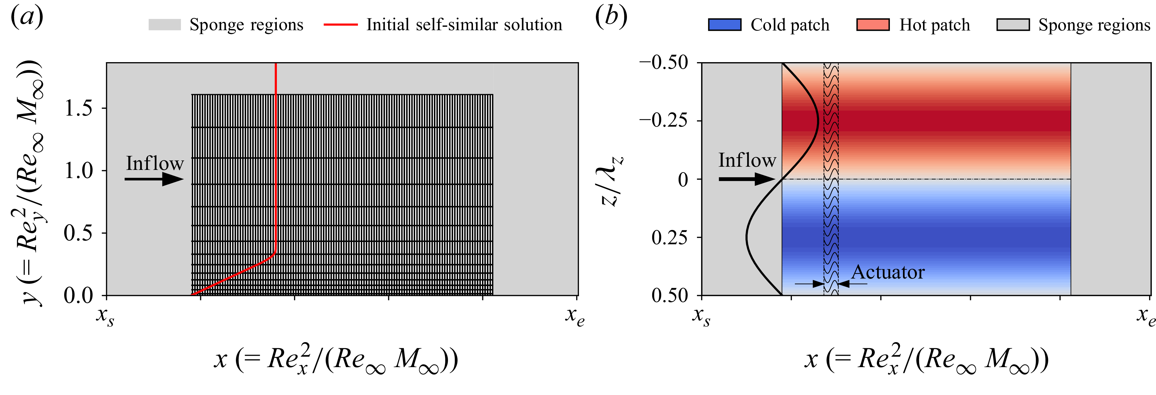


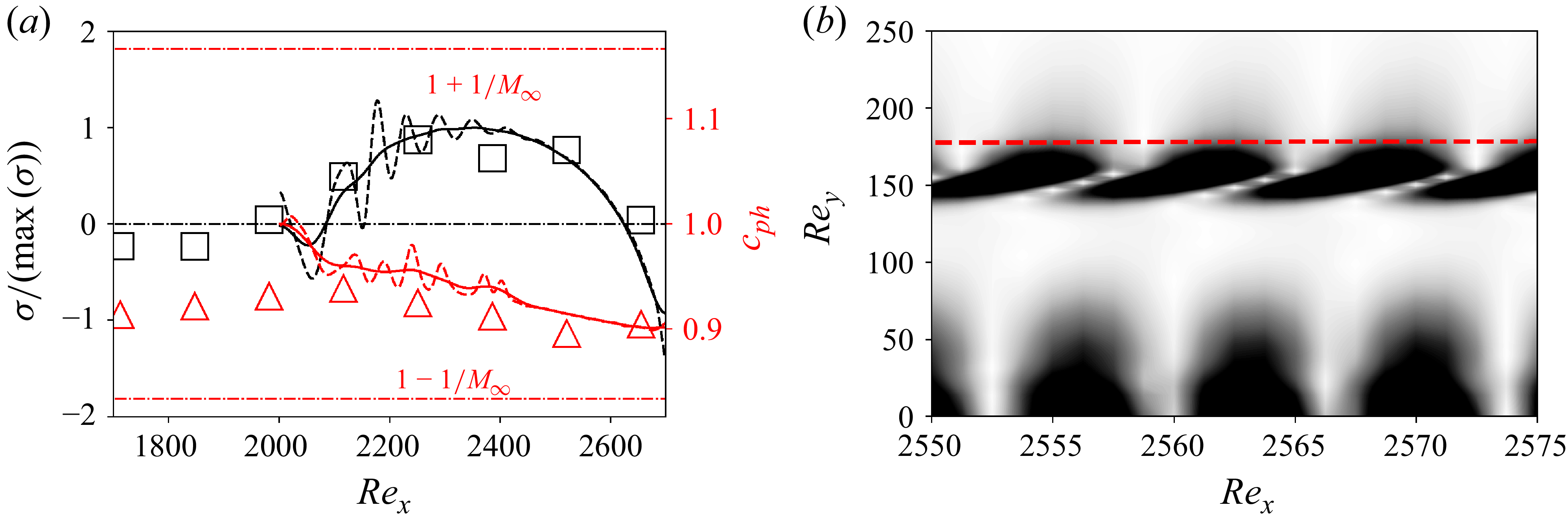


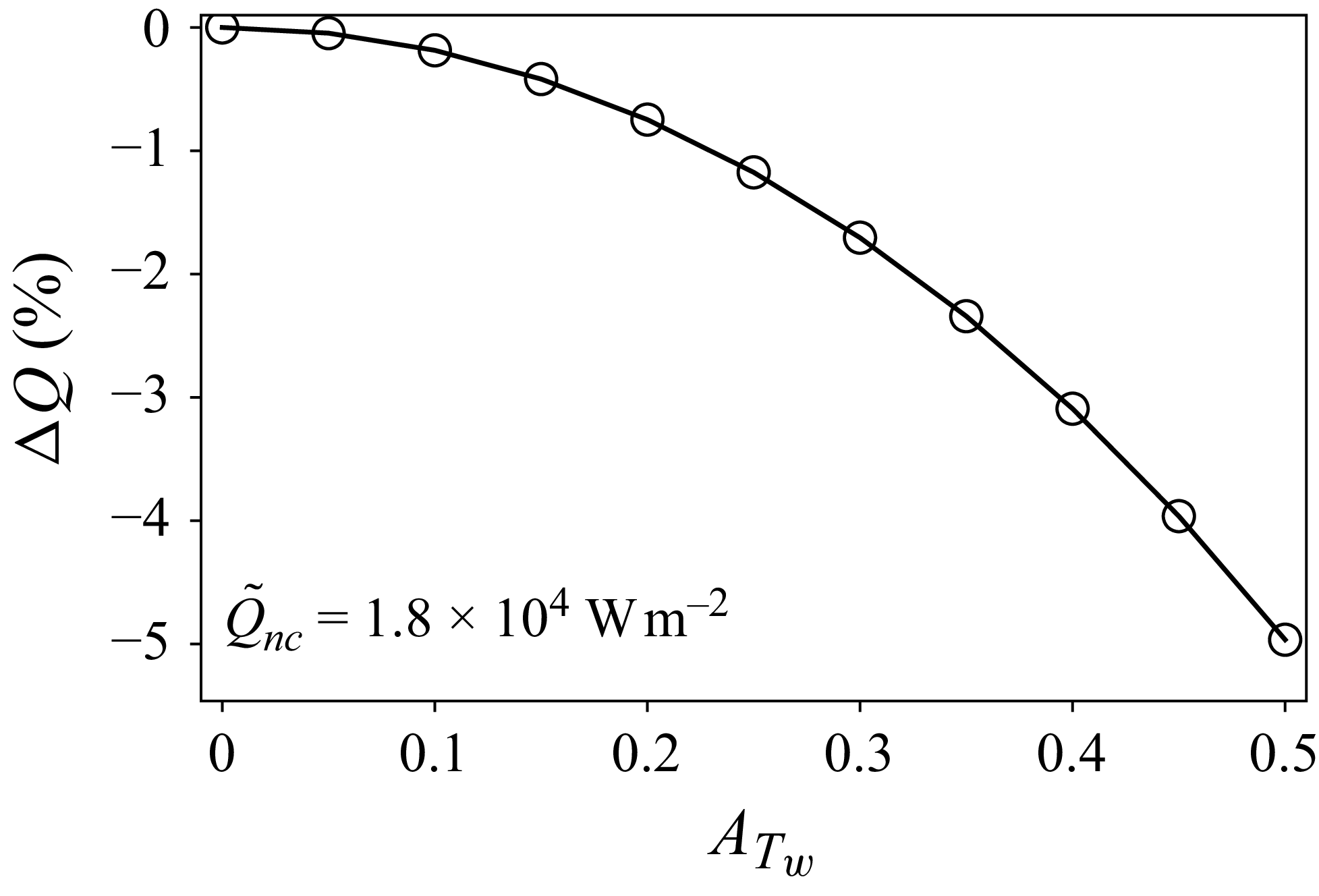


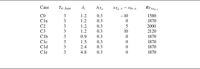


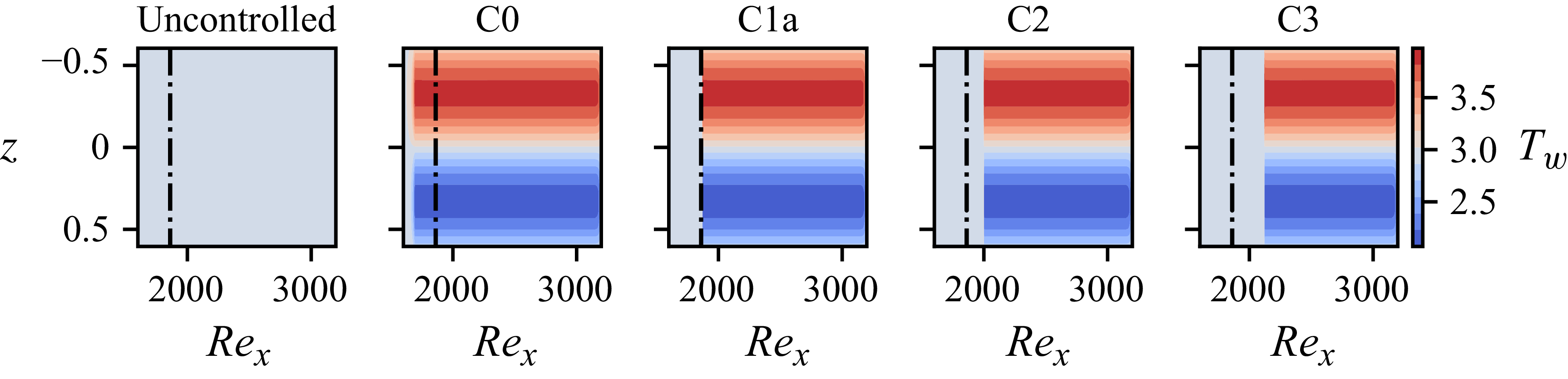


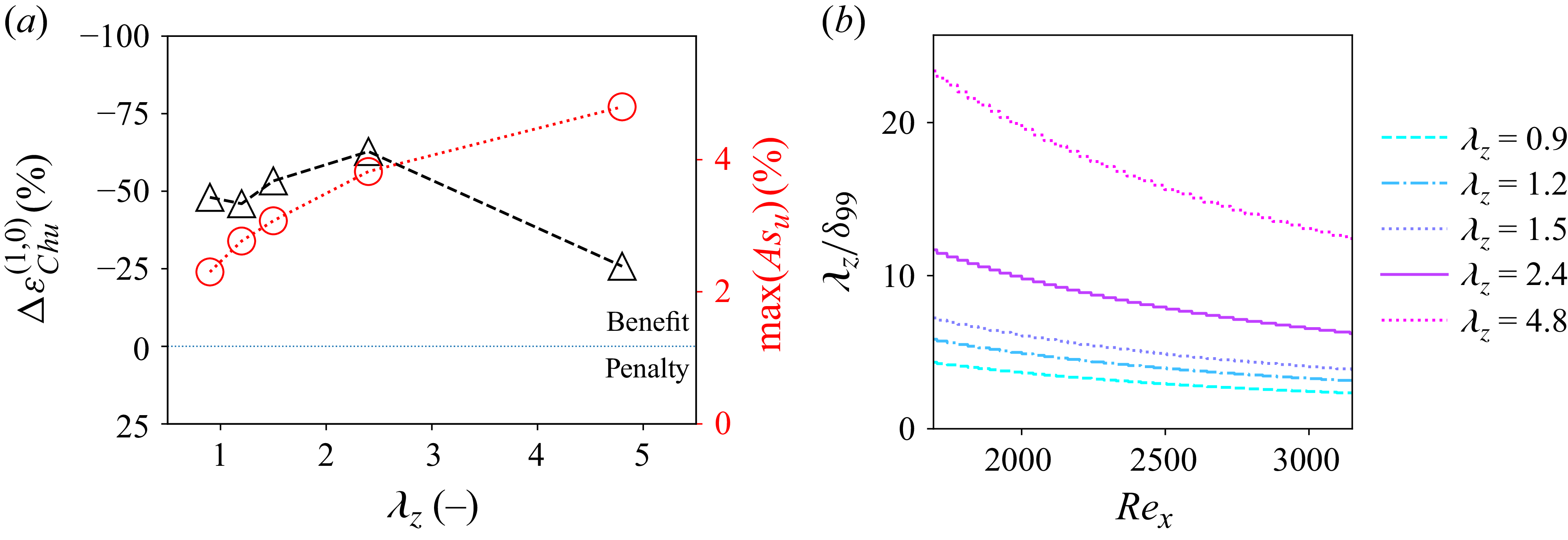


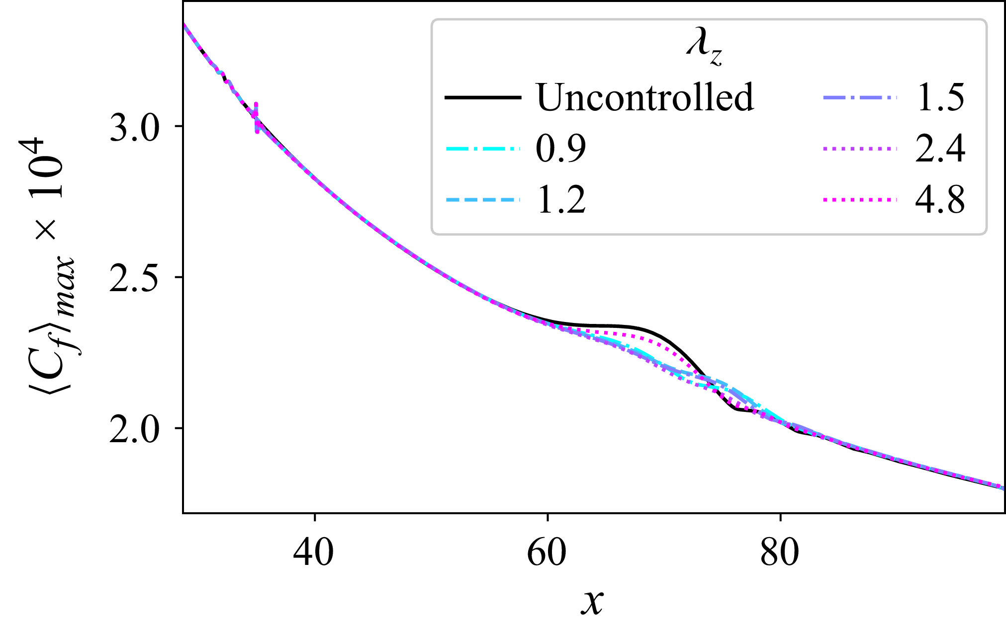


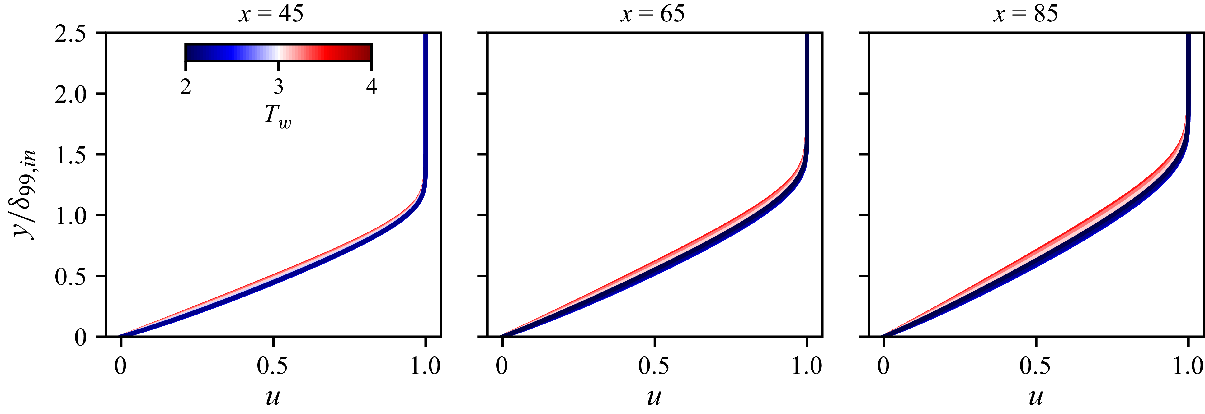


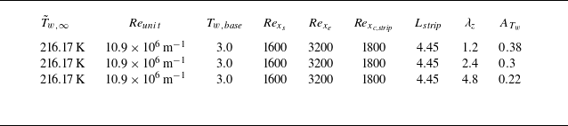


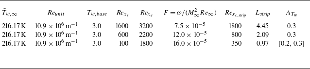


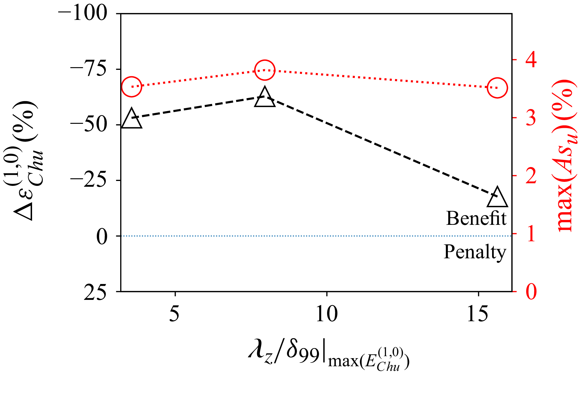

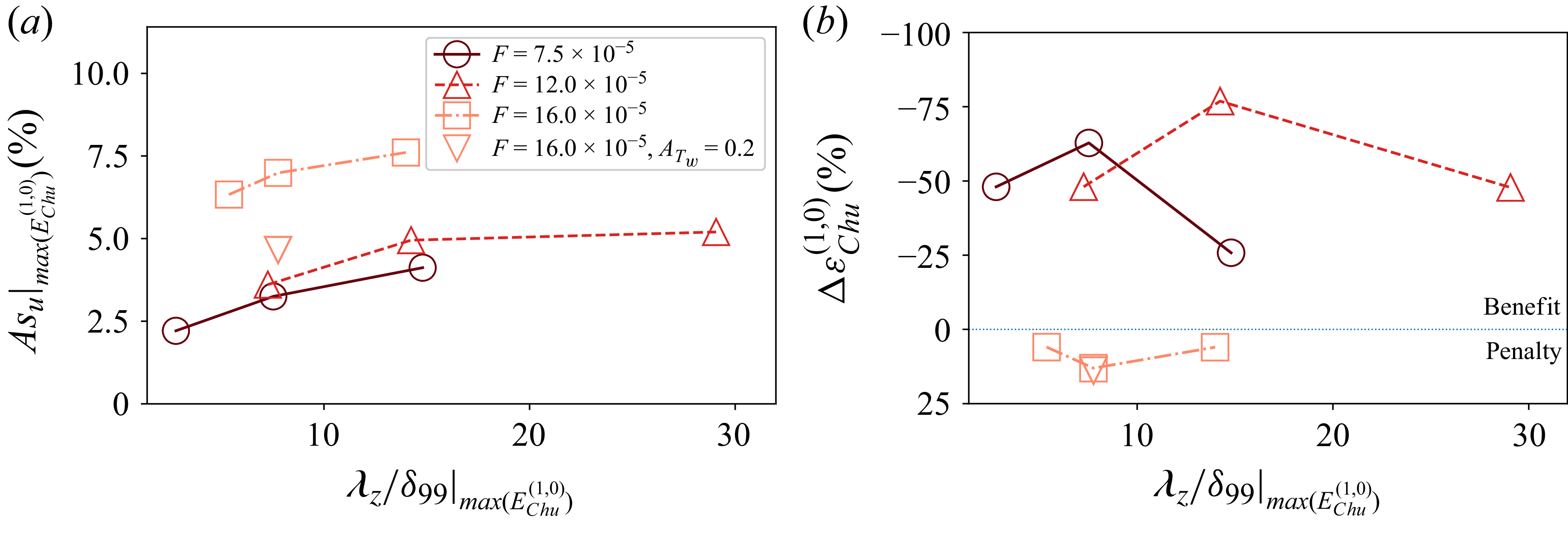


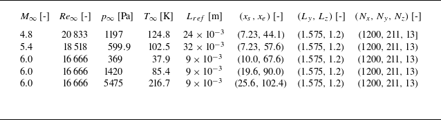
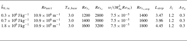


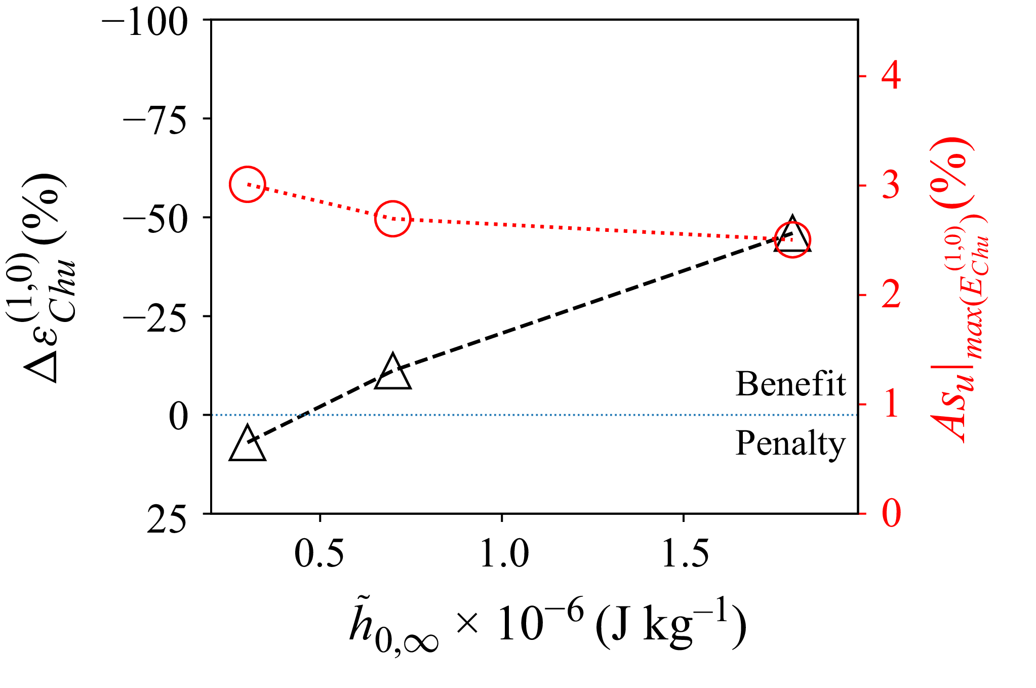


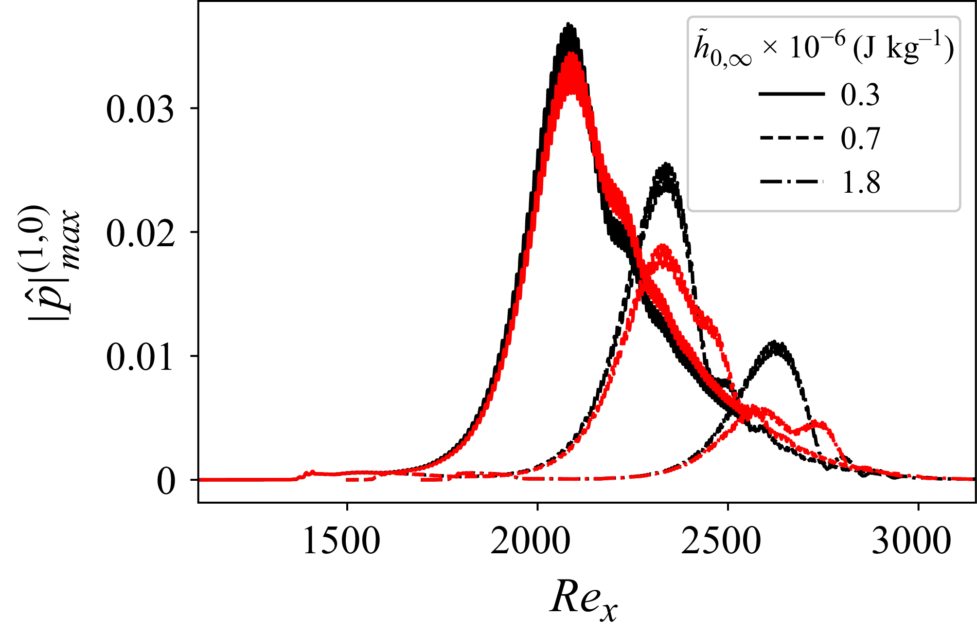

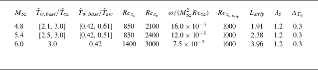


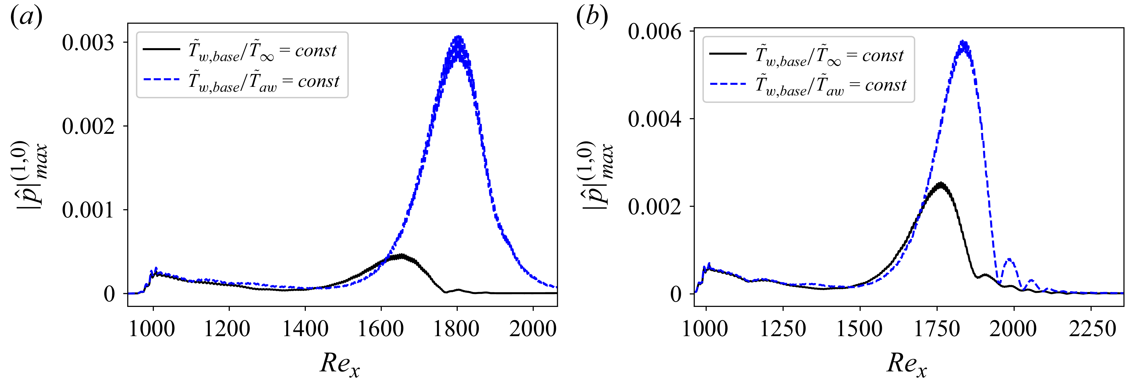


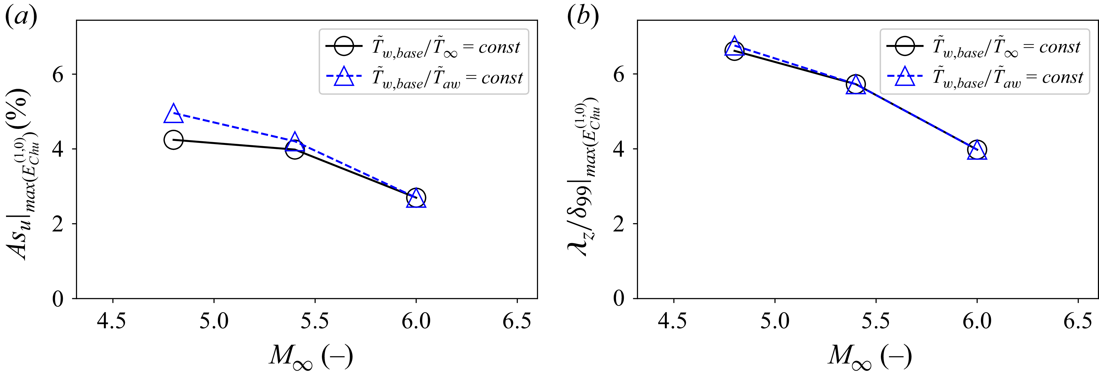

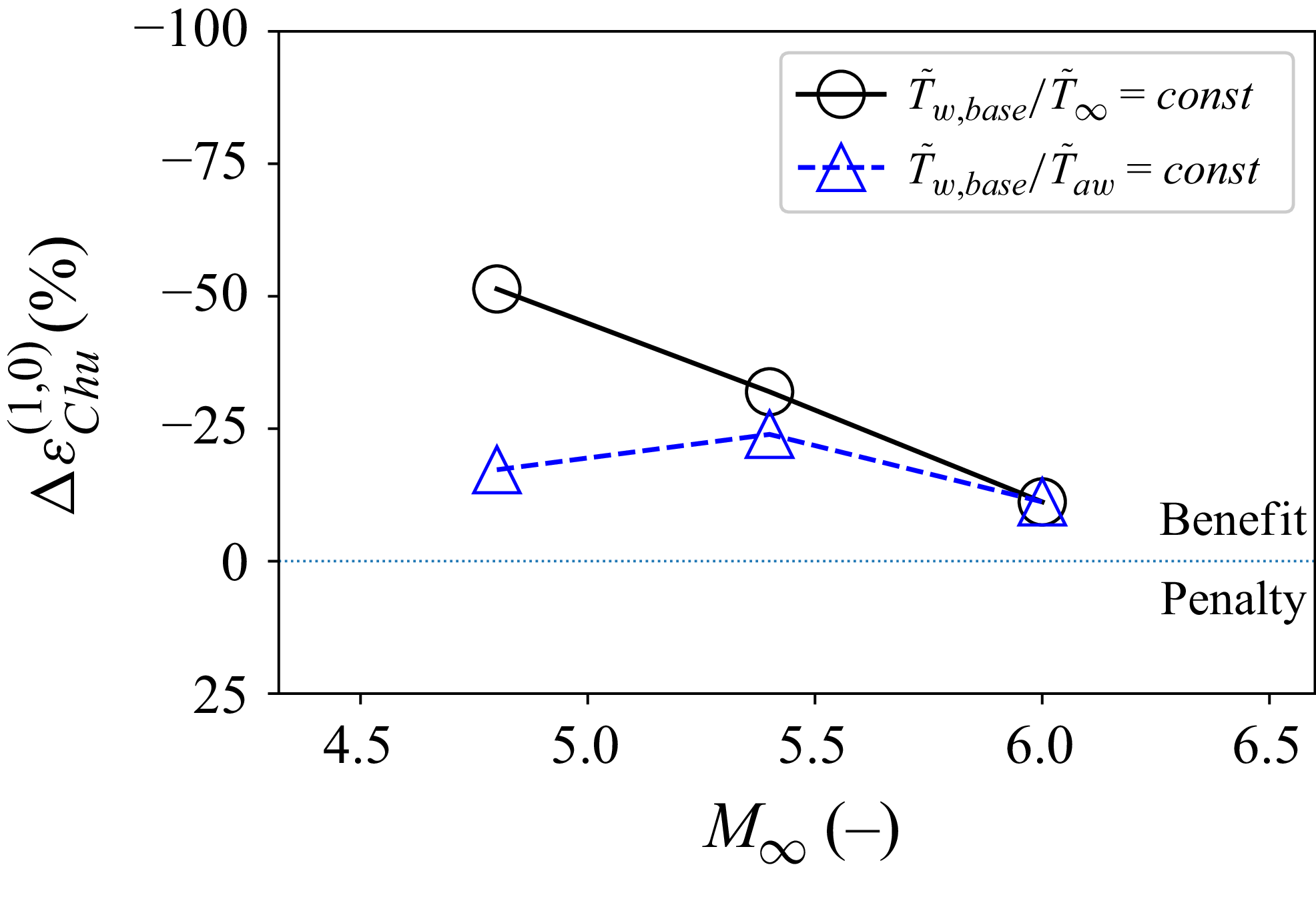

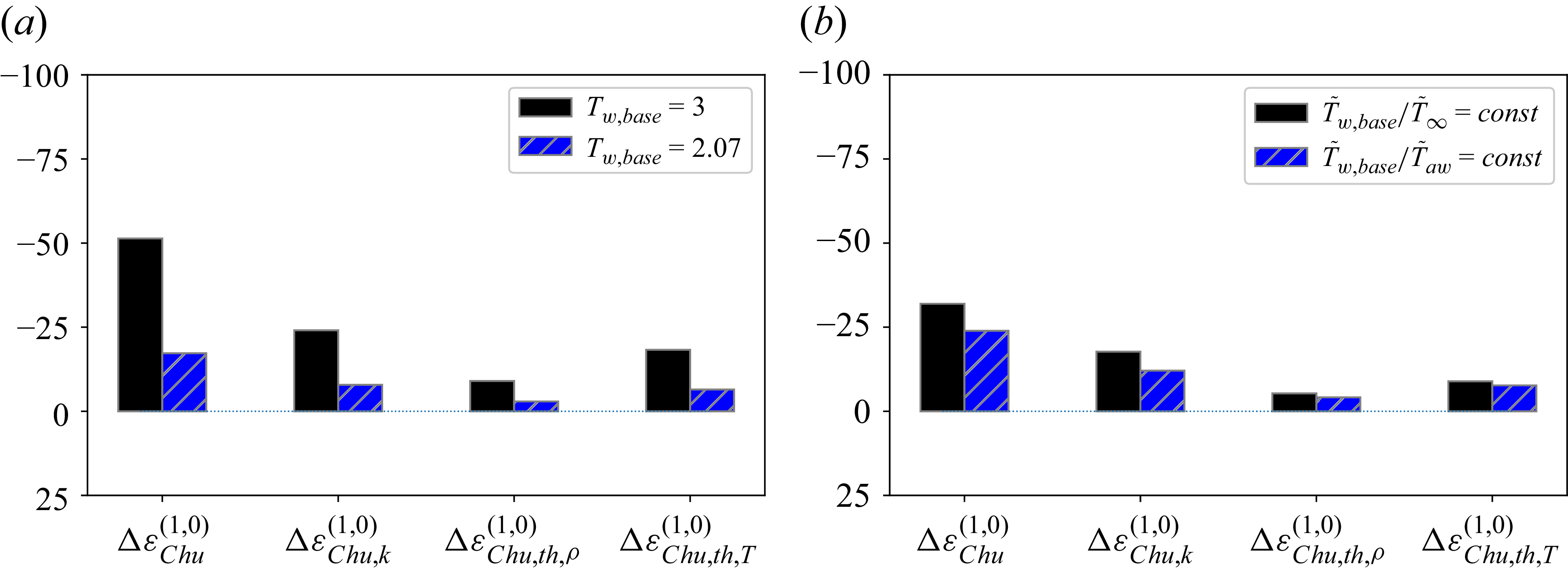


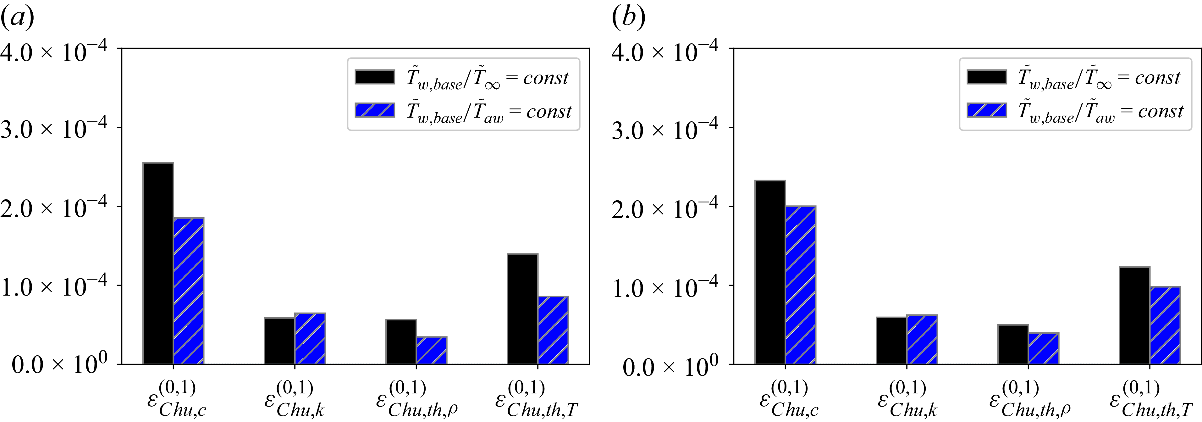


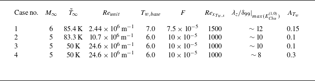

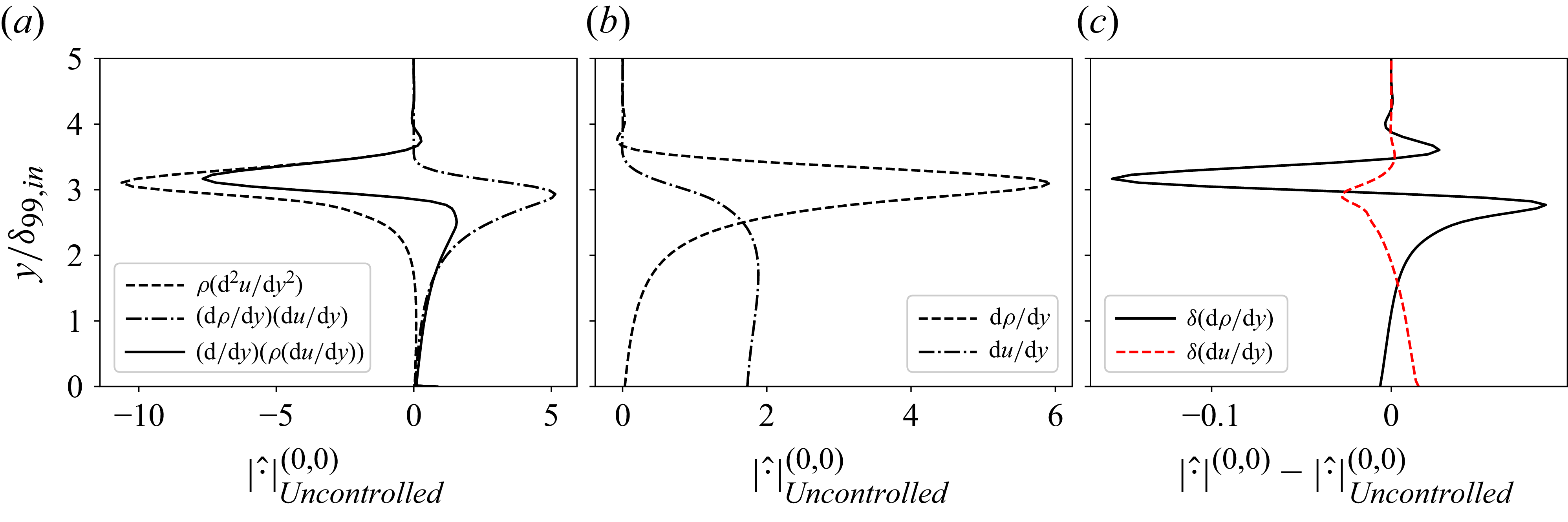


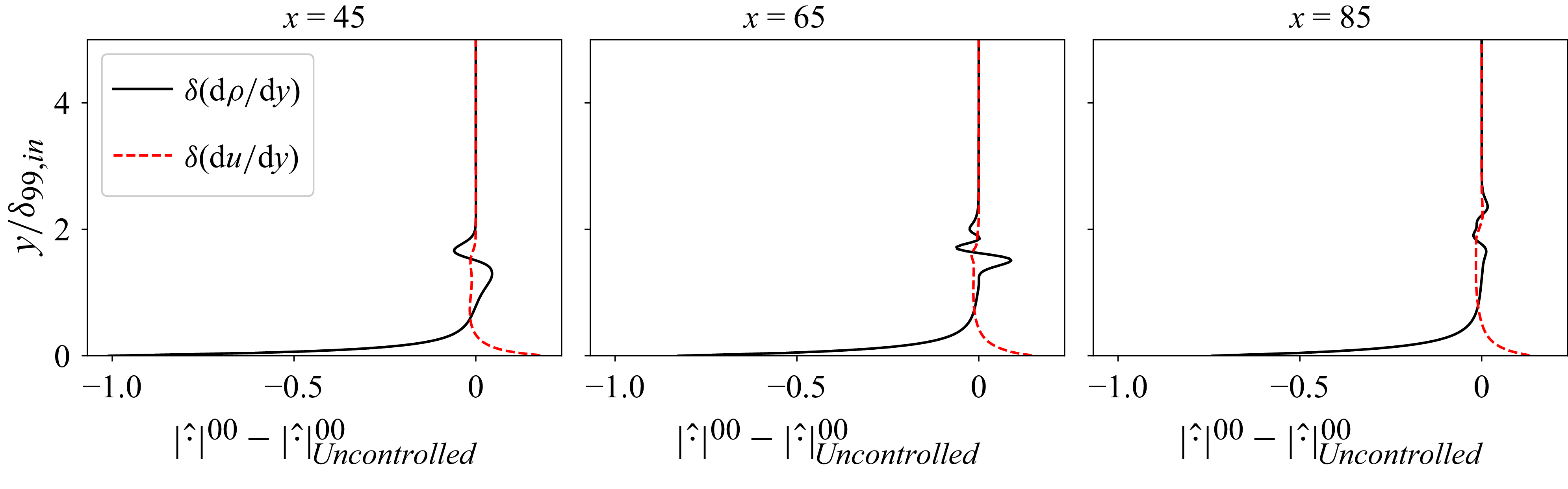


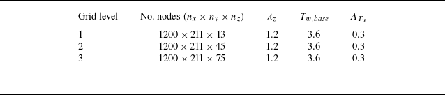


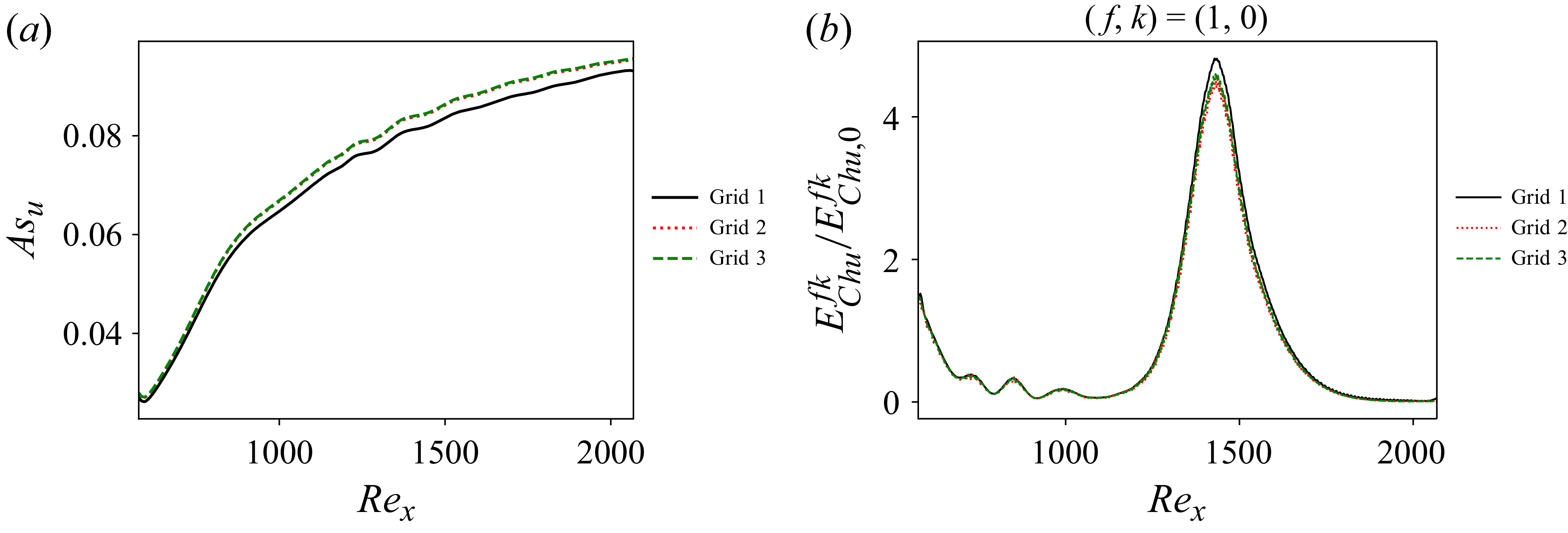


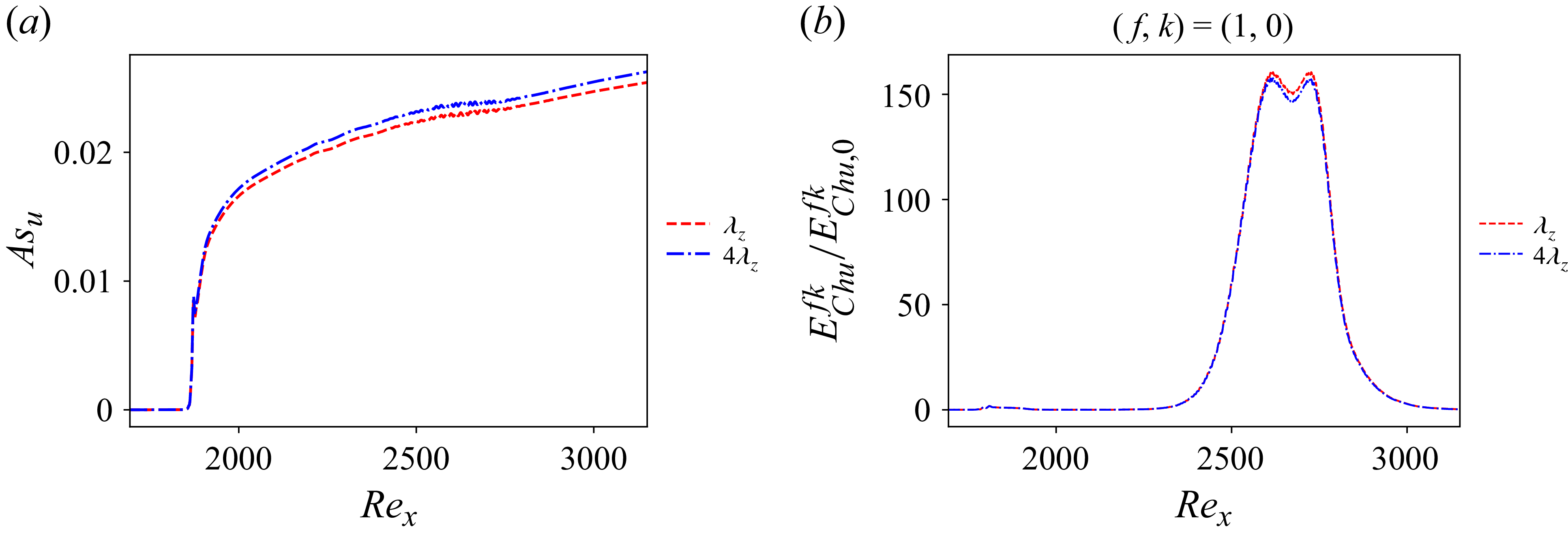


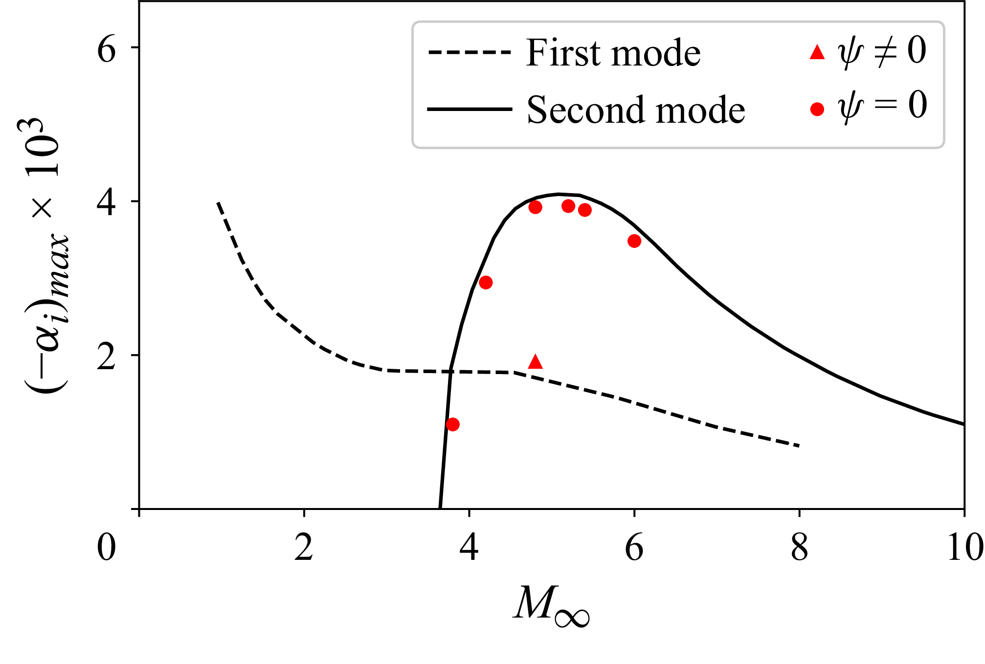


 Open access