


1. Introduction
In numerous applications, liquid is ejected or extruded out of a die or nozzle into air as a liquid sheet, e.g. in curtain coating, polymer processing and spraying (Middleman Reference Middleman1977; Kistler & Scriven Reference Kistler and Scriven1983; Lin Reference Lin2003), or a liquid jet, e.g. in inkjet printing (Basaran Reference Basaran2002; Lohse Reference Lohse2022). Dynamics of liquid sheets and liquid jets share similarities, but also differ in significant ways from one another. Liquid sheets that are of indefinitely large extent in the two directions perpendicular to the sheet thickness direction are linearly stable if sheet thickness is not of the order of micrometres or smaller. However, thinner sheets spontaneously rupture due to long-range, intermolecular van der Waals (vdW) forces (Ruckenstein & Jain Reference Ruckenstein and Jain1974; Vaynblat, Lister & Witelski Reference Vaynblat, Lister and Witelski2001; Thete et al. Reference Thete, Anthony, Doshi, Harris and Basaran2016; Garg et al. Reference Garg, Thete, Anthony and Basaran2022). In contrast, liquid jets are linearly unstable to long wavelength perturbations and disintegrate into drops by the capillary (Rayleigh–Plateau) instability without resorting to intermolecular forces (Anthony et al. Reference Anthony2023). In practice, however, liquid sheets are not infinite in extent, but have edges. These free edges of sheets move into them or retract due the unbalanced capillary (surface tension) pressure difference between the rounded edges and the planar portions of such sheets. The retraction dynamics is also affected by stresses owing to bulk as well as surface rheology. During retraction, sheets may disintegrate into filaments and drops or remain intact (see later). The goal of this work is to advance the understanding of the dynamics of sheet retraction when surface viscous effects are important.
Retraction of free edges of sheets, as well as how holes form in sheets and then grow by retraction of their edges, have long captivated the scientific community (Savart Reference Savart1833; Rayleigh Reference Rayleigh1891). Interest in the field grew rapidly after a set of papers by Dombrowski and co-workers (see, e.g. Dombrowski & Fraser Reference Dombrowski and Fraser1954), which contained strikingly beautiful photographs of disintegrating sheets, and the work of Ranz (Reference Ranz1959), and has continued unabated to this day (Lhuissier & Villermaux Reference Lhuissier and Villermaux2009). Taylor (Reference Taylor1959) and Culick (Reference Culick1960) independently showed theoretically that liquid sheets retract with a constant velocity now referred to as the Taylor–Culick velocity, $U_{\textit{TC}} \equiv (\sigma /\rho \tilde h_0)^{1/2}$
, where
$U_{\textit{TC}} \equiv (\sigma /\rho \tilde h_0)^{1/2}$
, where $\sigma$
,
$\sigma$
, $\rho$
and
$\rho$
and $\tilde h_0$
stand for surface tension, density and sheet half-thickness. Using the slender-sheet equations, Brenner & Gueyffier (Reference Brenner and Gueyffier1999) analysed the dynamics of retracting liquid sheets. Their work and subsequent studies showed that the dynamics falls into three regimes that depend on the Ohnesorge number
$\tilde h_0$
stand for surface tension, density and sheet half-thickness. Using the slender-sheet equations, Brenner & Gueyffier (Reference Brenner and Gueyffier1999) analysed the dynamics of retracting liquid sheets. Their work and subsequent studies showed that the dynamics falls into three regimes that depend on the Ohnesorge number $\textit{Oh} \equiv \mu /(\rho \tilde h_0 \sigma )^{1/2}$
, where
$\textit{Oh} \equiv \mu /(\rho \tilde h_0 \sigma )^{1/2}$
, where $\mu$
is viscosity. When
$\mu$
is viscosity. When $\textit{Oh}\lt 0.1$
, the retracting edge takes on the shape of a bulbous or circular rim and capillary waves form ahead of the rim. Subsequently, Sünderhauf et al. (Reference Sünderhauf, Raszillier and Durst2002) showed that in this regime, the rim retracts with a time-dependent velocity that asymptotically approaches
$\textit{Oh}\lt 0.1$
, the retracting edge takes on the shape of a bulbous or circular rim and capillary waves form ahead of the rim. Subsequently, Sünderhauf et al. (Reference Sünderhauf, Raszillier and Durst2002) showed that in this regime, the rim retracts with a time-dependent velocity that asymptotically approaches $U_{\textit{TC}}$
. As the amplitude of the capillary waves can be large, Burton & Taborek (Reference Burton and Taborek2007) showed that retracting sheets can exhibit a finite-time pinch-off singularity and break even in the absence of vdW forces when the liquid is inviscid (
$U_{\textit{TC}}$
. As the amplitude of the capillary waves can be large, Burton & Taborek (Reference Burton and Taborek2007) showed that retracting sheets can exhibit a finite-time pinch-off singularity and break even in the absence of vdW forces when the liquid is inviscid ( $\textit{Oh} = 0$
). Recently, however, Wee et al. (Reference Wee, Kumar, Liu and Basaran2024b
) demonstrated that liquid sheets of small but finite viscosity (
$\textit{Oh} = 0$
). Recently, however, Wee et al. (Reference Wee, Kumar, Liu and Basaran2024b
) demonstrated that liquid sheets of small but finite viscosity ( $\textit{Oh} \ll 1$
) will escape pinch-off if vdW forces are absent. As
$\textit{Oh} \ll 1$
) will escape pinch-off if vdW forces are absent. As $\textit{Oh}$
increases, Brenner & Gueyffier (Reference Brenner and Gueyffier1999) reported that a rim, albeit a non-circular one, still arises during retraction but without the formation of capillary waves. When
$\textit{Oh}$
increases, Brenner & Gueyffier (Reference Brenner and Gueyffier1999) reported that a rim, albeit a non-circular one, still arises during retraction but without the formation of capillary waves. When $\textit{Oh}$
is sufficiently large, no rim whatsoever forms and the film remains flat away from the tip. Studies in this latter regime have determined the evolution in time
$\textit{Oh}$
is sufficiently large, no rim whatsoever forms and the film remains flat away from the tip. Studies in this latter regime have determined the evolution in time $\tilde t$
of the maximum film half-thickness
$\tilde t$
of the maximum film half-thickness $\tilde {h}_m$
, tip speed and sheet length (Savva & Bush Reference Savva and Bush2009; Deka & Pierson Reference Deka and Pierson2020). Exploiting the uniformity of the film profile outside of the tip region, Savva & Bush (Reference Savva and Bush2009) obtained the analytical expression
$\tilde {h}_m$
, tip speed and sheet length (Savva & Bush Reference Savva and Bush2009; Deka & Pierson Reference Deka and Pierson2020). Exploiting the uniformity of the film profile outside of the tip region, Savva & Bush (Reference Savva and Bush2009) obtained the analytical expression
 \begin{equation} \tilde {h}_m/\tilde {h}_0 = 1 + (\sigma / 4 \mu \tilde {h}_0 ) \ \tilde {t}. \end{equation}
Equation (1.1) accurately predicts the time evolution of $\tilde {h}_m$
in the early stages of retraction and can be used to infer the tip speed by using volume conservation.
$\tilde {h}_m$
in the early stages of retraction and can be used to infer the tip speed by using volume conservation.
Retraction of three-dimensional (3-D) but axisymmetric (3-DA) filaments (elongated drops), like liquid sheets (slender two-dimensional (2-D) drops), is also driven by capillary pressure. Thus, the former has a number of implications for the latter (Anthony et al. Reference Anthony, Kamat, Harris and Basaran2019; Pierson et al. Reference Pierson, Magnaudet, Soares and Popinet2020). The retraction dynamics of 3-DA filaments is found sometimes to be impacted in unexpected ways by both bulk and interfacial stresses. Sen et al. (Reference Sen, Datt, Segers, Wijshoff, Snoeijer, Versluis and Lohse2021) have shown that viscoelastic stresses due to prestretching of polymer molecules can greatly increase recoil speed (see also Liu, Wagoner & Basaran Reference Liu, Wagoner and Basaran2022). Surface-active species, which not only reduce surface tension, but also give rise to surface tension gradients, and hence Marangoni stresses, and surface rheological (viscous) stresses (Scriven & Sternling Reference Scriven and Sternling1964), can profoundly affect recoil (De Corato et al. Reference De Corato, Tammaro, Maffettone and Fueyo2022). Kamat et al. (Reference Kamat, Wagoner, Castrejón-Pita, Castrejón-Pita, Anthony and Basaran2020b
) have shown that 3-DA filaments covered with surfactants can escape pinch-off during retraction due to Marangoni stresses. Recent studies have demonstrated that certain Newtonian fluids whose interfaces are devoid of surfactants can nevertheless exhibit surface viscous effects due to the formation of a thin oxide layer at their interfaces (Lyubimov et al. Reference Lyubimov, Konovalov, Lyubimova and Egry2011; Elton et al. Reference Elton, Reeve, Thornley, Joshipura, Paul, Pascall and Jeffries2020; Malgaretti et al. Reference Malgaretti, Bafile, Vallauri, Jedlovszky and Sega2023). Oxide layers at the interfaces of liquid metals impart an intrinsic viscous nature to the surface which can be characterised by an intrinsic constant surface viscosity. Given the current interest in the use of molten metal droplets in applications, e.g. chip fabrication (Versolato et al. Reference Versolato, Sheil, Witte, Ubachs and Hoekstra2022), and the long-standing importance of surfactants in spraying (Dombrowski & Fraser Reference Dombrowski and Fraser1954) and jetting (Lohse Reference Lohse2022), we investigate how surface viscosity can affect a free surface flow involving the retraction dynamics of liquid sheets when $\textit{Oh} \gg 1$
.
$\textit{Oh} \gg 1$
.
2. Problem formulation and numerical method
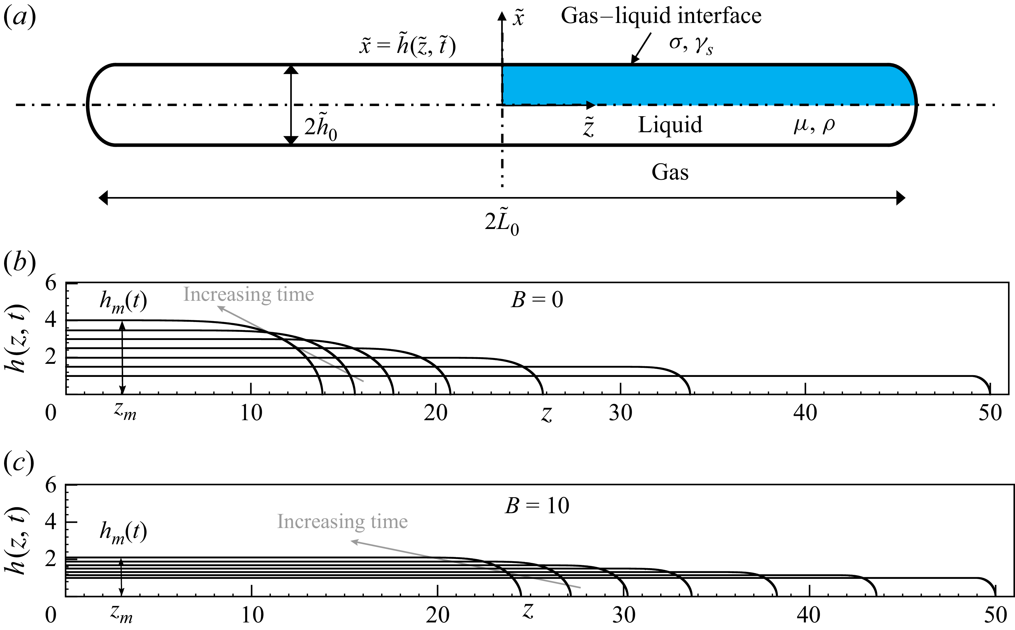
Schematic and instantaneous profiles of contracting liquid sheets. (a) Definition sketch showing the cross-section of the sheet (2-D drop) at $\tilde t=0$
. Because of symmetry, the problem domain is only one-quarter of the cross-section (shaded in blue). (b, c) Instantaneous shapes of a retracting sheet of initial half-length
$\tilde t=0$
. Because of symmetry, the problem domain is only one-quarter of the cross-section (shaded in blue). (b, c) Instantaneous shapes of a retracting sheet of initial half-length $L_0=50$
and
$L_0=50$
and $\textit{Oh}=1000$
: (b)
$\textit{Oh}=1000$
: (b) ${B}=0$
(surface viscosity is absent) and (c)
${B}=0$
(surface viscosity is absent) and (c) ${B}=10$
(surface viscosity is present). Shape profiles are shown at constant intervals of dimensionless time
${B}=10$
(surface viscosity is present). Shape profiles are shown at constant intervals of dimensionless time $\Delta t \approx 2$
for
$\Delta t \approx 2$
for $0 \le t \le 12$
. In both cases, the film remains nearly flat away from the circular tips. When
$0 \le t \le 12$
. In both cases, the film remains nearly flat away from the circular tips. When ${B}=10$
, the film thickens and the sheet recoils more slowly compared with when
${B}=10$
, the film thickens and the sheet recoils more slowly compared with when ${B}=0$
.
${B}=0$
.

The system (figure 1
a) consists of an isothermal Newtonian liquid sheet that undergoes incompressible flow and is surrounded by a dynamically passive gas which exerts a constant pressure on the liquid. The sheet’s density $\rho$
and bulk viscosity
$\rho$
and bulk viscosity $\mu$
are constants. Initially, the sheet’s two parallel surfaces are separated by
$\mu$
are constants. Initially, the sheet’s two parallel surfaces are separated by $2 \tilde {h}_0$
and capped by two semicircles of radii
$2 \tilde {h}_0$
and capped by two semicircles of radii $\tilde {h}_0$
. The distance between the tips is
$\tilde {h}_0$
. The distance between the tips is $2 \tilde {L}_0$
. The surface tension
$2 \tilde {L}_0$
. The surface tension $\sigma$
of the air–liquid interface is constant. Apart from surface tension, the interface is a compressible 2-D phase characterised by intrinsic shear and dilatational surface viscosities
$\sigma$
of the air–liquid interface is constant. Apart from surface tension, the interface is a compressible 2-D phase characterised by intrinsic shear and dilatational surface viscosities $\gamma ^s_s$
and
$\gamma ^s_s$
and $\gamma ^d_s$
, both of which are constants and differ from the bulk viscosity.
$\gamma ^d_s$
, both of which are constants and differ from the bulk viscosity.
Here, it is convenient to use a Cartesian coordinate system $(\tilde x, \tilde y, \tilde z)$
that is based at the centre of the sheet or 2-D drop: the
$(\tilde x, \tilde y, \tilde z)$
that is based at the centre of the sheet or 2-D drop: the $\tilde x$
and
$\tilde x$
and $\tilde z$
axes point in the sheet thickness and lateral directions (figure 1
a) and the sheet is taken to be indefinitely long in the
$\tilde z$
axes point in the sheet thickness and lateral directions (figure 1
a) and the sheet is taken to be indefinitely long in the $\tilde y$
direction (which points out of the page). It is assumed herein that the dynamics remains symmetric at all times with respect to the
$\tilde y$
direction (which points out of the page). It is assumed herein that the dynamics remains symmetric at all times with respect to the $\tilde {x}=0$
and
$\tilde {x}=0$
and $\tilde {z}=0$
midplanes.
$\tilde {z}=0$
midplanes.
A Newtonian fluid sheet of instantaneous length $2 \tilde {L}(\tilde {t})$
starts to recoil at
$2 \tilde {L}(\tilde {t})$
starts to recoil at $\tilde {t}=0$
due to the difference in capillary pressure in the circular caps and the flat portion of the sheet far from the tips. The dynamics of this free boundary problem is governed by the continuity equation
$\tilde {t}=0$
due to the difference in capillary pressure in the circular caps and the flat portion of the sheet far from the tips. The dynamics of this free boundary problem is governed by the continuity equation $\tilde {\boldsymbol{\nabla }} \boldsymbol{\cdot }\tilde {\boldsymbol{v}} = 0$
and the Navier Stokes equations
$\tilde {\boldsymbol{\nabla }} \boldsymbol{\cdot }\tilde {\boldsymbol{v}} = 0$
and the Navier Stokes equations $\rho ( \partial \tilde {\boldsymbol{v}}/\partial \tilde {t} + \tilde {\boldsymbol{v}} \boldsymbol{\cdot }\tilde {\boldsymbol{\nabla }} \tilde {\boldsymbol{v}} ) = \tilde {\boldsymbol{\nabla }} \boldsymbol{\cdot }\boldsymbol{\tilde {T}}$
. Here,
$\rho ( \partial \tilde {\boldsymbol{v}}/\partial \tilde {t} + \tilde {\boldsymbol{v}} \boldsymbol{\cdot }\tilde {\boldsymbol{\nabla }} \tilde {\boldsymbol{v}} ) = \tilde {\boldsymbol{\nabla }} \boldsymbol{\cdot }\boldsymbol{\tilde {T}}$
. Here, $\boldsymbol{\tilde {T}} = -\tilde {p} \boldsymbol{I} + \mu [ \tilde {\boldsymbol{\nabla }} \tilde {\boldsymbol{v}} + (\tilde {\boldsymbol{\nabla }} \tilde {\boldsymbol{v}})^T ]$
is the total stress tensor in the bulk Newtonian liquid where the fluid velocity
$\boldsymbol{\tilde {T}} = -\tilde {p} \boldsymbol{I} + \mu [ \tilde {\boldsymbol{\nabla }} \tilde {\boldsymbol{v}} + (\tilde {\boldsymbol{\nabla }} \tilde {\boldsymbol{v}})^T ]$
is the total stress tensor in the bulk Newtonian liquid where the fluid velocity $\tilde {\boldsymbol{v}} = \tilde {u} \boldsymbol{e}_x + \tilde {v} \boldsymbol{e}_z$
, with
$\tilde {\boldsymbol{v}} = \tilde {u} \boldsymbol{e}_x + \tilde {v} \boldsymbol{e}_z$
, with $\boldsymbol{e}_x$
and
$\boldsymbol{e}_x$
and $\boldsymbol{e}_z$
denoting the unit vectors defined along the
$\boldsymbol{e}_z$
denoting the unit vectors defined along the $\tilde {x}$
and
$\tilde {x}$
and $\tilde {z}$
directions, and
$\tilde {z}$
directions, and $\tilde {u}$
and
$\tilde {u}$
and $\tilde {v}$
denoting the
$\tilde {v}$
denoting the $\tilde {x}$
and
$\tilde {x}$
and $\tilde {z}$
components of fluid velocity. Here,
$\tilde {z}$
components of fluid velocity. Here, $\tilde {p}$
is the pressure and
$\tilde {p}$
is the pressure and $\boldsymbol{I}$
is the identity tensor. The free surface
$\boldsymbol{I}$
is the identity tensor. The free surface $S(\tilde t)$
separating the interior of the sheet from its exterior is described by the curve
$S(\tilde t)$
separating the interior of the sheet from its exterior is described by the curve $\tilde {x}=\tilde {h}(\tilde {z},\tilde {t})$
, where
$\tilde {x}=\tilde {h}(\tilde {z},\tilde {t})$
, where $\tilde h$
is the interface shape function. Conservation of mass along
$\tilde h$
is the interface shape function. Conservation of mass along $S(\tilde t)$
is guaranteed by the kinematic boundary condition,
$S(\tilde t)$
is guaranteed by the kinematic boundary condition, $\tilde {u} = \partial \tilde {h}/\partial \tilde {t} + \tilde {v} \, (\partial \tilde {h}/\partial \tilde {z})$
, and conservation of momentum along
$\tilde {u} = \partial \tilde {h}/\partial \tilde {t} + \tilde {v} \, (\partial \tilde {h}/\partial \tilde {z})$
, and conservation of momentum along $S(\tilde t)$
by the traction boundary condition. Here, the Boussinesq–Scriven constitutive equation (hereafter, BSCE) is adopted to describe surface rheological effects (Scriven Reference Scriven1960) such that the traction boundary condition becomes
$S(\tilde t)$
by the traction boundary condition. Here, the Boussinesq–Scriven constitutive equation (hereafter, BSCE) is adopted to describe surface rheological effects (Scriven Reference Scriven1960) such that the traction boundary condition becomes $ \boldsymbol{n} \boldsymbol{\cdot }\boldsymbol{\tilde {T}}= 2 \tilde {\mathcal{H}} \sigma \boldsymbol{n}+\tilde {\boldsymbol{\nabla} }_s \sigma +2 \tilde {\mathcal{H}} (\gamma _s^d-\gamma ^s_s ) (\tilde {\boldsymbol{\nabla} }_s \boldsymbol{\cdot }\tilde {\boldsymbol{v}} ) \boldsymbol{n} +\tilde {\boldsymbol{\nabla} }_s [ (\gamma _s^d-\gamma ^s_s ) (\tilde {\boldsymbol{\nabla} }_s \boldsymbol{\cdot }\tilde {\boldsymbol{v}} ) ]+\tilde {\boldsymbol{\nabla} }_s \boldsymbol{\cdot }[\gamma ^s_s (\tilde {\boldsymbol{\nabla} }_s \tilde {\boldsymbol{v}} \boldsymbol{\cdot }\boldsymbol{I}^s+\boldsymbol{I}^s \boldsymbol{\cdot }(\tilde {\boldsymbol{\nabla} }_s \tilde {\boldsymbol{v}} )^T ) ]$
. Here,
$ \boldsymbol{n} \boldsymbol{\cdot }\boldsymbol{\tilde {T}}= 2 \tilde {\mathcal{H}} \sigma \boldsymbol{n}+\tilde {\boldsymbol{\nabla} }_s \sigma +2 \tilde {\mathcal{H}} (\gamma _s^d-\gamma ^s_s ) (\tilde {\boldsymbol{\nabla} }_s \boldsymbol{\cdot }\tilde {\boldsymbol{v}} ) \boldsymbol{n} +\tilde {\boldsymbol{\nabla} }_s [ (\gamma _s^d-\gamma ^s_s ) (\tilde {\boldsymbol{\nabla} }_s \boldsymbol{\cdot }\tilde {\boldsymbol{v}} ) ]+\tilde {\boldsymbol{\nabla} }_s \boldsymbol{\cdot }[\gamma ^s_s (\tilde {\boldsymbol{\nabla} }_s \tilde {\boldsymbol{v}} \boldsymbol{\cdot }\boldsymbol{I}^s+\boldsymbol{I}^s \boldsymbol{\cdot }(\tilde {\boldsymbol{\nabla} }_s \tilde {\boldsymbol{v}} )^T ) ]$
. Here, $\boldsymbol{n}$
is the outward pointing normal to
$\boldsymbol{n}$
is the outward pointing normal to $S(\tilde t)$
,
$S(\tilde t)$
, $\boldsymbol{I}^s \equiv \boldsymbol{I} - \boldsymbol{n} \boldsymbol{n}$
the surface identity tensor,
$\boldsymbol{I}^s \equiv \boldsymbol{I} - \boldsymbol{n} \boldsymbol{n}$
the surface identity tensor, $\tilde {\boldsymbol{\nabla} }_s=\boldsymbol{I}^s \boldsymbol{\cdot }\tilde {\boldsymbol{\nabla }}$
the surface gradient operator and
$\tilde {\boldsymbol{\nabla} }_s=\boldsymbol{I}^s \boldsymbol{\cdot }\tilde {\boldsymbol{\nabla }}$
the surface gradient operator and $2 \mathcal{\tilde {H}} = -\tilde {\boldsymbol{\nabla} }_s \boldsymbol{\cdot }\boldsymbol{n}$
twice the mean curvature. The first term on the right-hand side of the BSCE corresponds to the capillary pressure, the second term corresponds to stresses induced by surface tension gradients (Marangoni stresses) and the remaining terms account for the surface viscous effects. As
$2 \mathcal{\tilde {H}} = -\tilde {\boldsymbol{\nabla} }_s \boldsymbol{\cdot }\boldsymbol{n}$
twice the mean curvature. The first term on the right-hand side of the BSCE corresponds to the capillary pressure, the second term corresponds to stresses induced by surface tension gradients (Marangoni stresses) and the remaining terms account for the surface viscous effects. As $\sigma$
and both
$\sigma$
and both $\gamma _s^s$
and
$\gamma _s^s$
and $\gamma _s^d$
are constants in this work, in the Cartesian coordinate system, the BSCE simplifies so that
$\gamma _s^d$
are constants in this work, in the Cartesian coordinate system, the BSCE simplifies so that $\boldsymbol{n} \boldsymbol{\cdot }\boldsymbol{\tilde {T}} = 2 \mathcal{\tilde {H}} \sigma \boldsymbol{n} + 2 \mathcal{\tilde {H}} (\gamma _s^s + \gamma _s^d ) (\tilde {\boldsymbol{\nabla} }_s \boldsymbol{\cdot }\tilde {\boldsymbol{v}} ) \boldsymbol{n} + (\gamma _s^s + \gamma _s^d ) [ \tilde {\boldsymbol{\nabla} }_s (\tilde {\boldsymbol{\nabla} }_s \boldsymbol{\cdot }\tilde {\boldsymbol{v}} ) ]$
. As has already been noted by Wee et al. (Reference Wee, Wagoner and Basaran2022b
), in Cartesian coordinates, the two surface viscosities always appear grouped together. Hence, it is expedient to define the intrinsic surface viscosity
$\boldsymbol{n} \boldsymbol{\cdot }\boldsymbol{\tilde {T}} = 2 \mathcal{\tilde {H}} \sigma \boldsymbol{n} + 2 \mathcal{\tilde {H}} (\gamma _s^s + \gamma _s^d ) (\tilde {\boldsymbol{\nabla} }_s \boldsymbol{\cdot }\tilde {\boldsymbol{v}} ) \boldsymbol{n} + (\gamma _s^s + \gamma _s^d ) [ \tilde {\boldsymbol{\nabla} }_s (\tilde {\boldsymbol{\nabla} }_s \boldsymbol{\cdot }\tilde {\boldsymbol{v}} ) ]$
. As has already been noted by Wee et al. (Reference Wee, Wagoner and Basaran2022b
), in Cartesian coordinates, the two surface viscosities always appear grouped together. Hence, it is expedient to define the intrinsic surface viscosity $\gamma _s$
as their sum, viz. to set
$\gamma _s$
as their sum, viz. to set $\gamma _s \equiv \gamma _s^s + \gamma _s^d$
in the BSCE. Therefore,
$\gamma _s \equiv \gamma _s^s + \gamma _s^d$
in the BSCE. Therefore,
 \begin{equation} \boldsymbol{n} \boldsymbol{\cdot }\boldsymbol{\tilde {T}} = 2 \mathcal{\tilde {H}} \sigma \boldsymbol{n} + 2 \mathcal{\tilde {H}} \gamma _s \big (\tilde {\boldsymbol{\nabla} }_s \boldsymbol{\cdot }\tilde {\boldsymbol{v}} \big ) \boldsymbol{n} + \gamma _s \big [ \tilde {\boldsymbol{\nabla} }_s \big (\tilde {\boldsymbol{\nabla} }_s \boldsymbol{\cdot }\tilde {\boldsymbol{v}} \big ) \big ]. \end{equation}
We next derive a set of slender-sheet equations when surface viscosity is constant using the averaging method that was used by Timmermans & Lister (Reference Timmermans and Lister2002) in their analysis of dynamics of surfactant-covered liquid jets albeit in the absence of surface viscosity. In what follows, we denote the cross-section average of any field variable $(\boldsymbol{\cdot })$
as
$(\boldsymbol{\cdot })$
as $\overline {(\boldsymbol{\cdot })} = ({1}/{\tilde {h}}) \int _0^{\tilde {h}} \tilde {(\boldsymbol{\cdot })} \, {\rm d} \tilde {x}$
. Hence, the averaged continuity and
$\overline {(\boldsymbol{\cdot })} = ({1}/{\tilde {h}}) \int _0^{\tilde {h}} \tilde {(\boldsymbol{\cdot })} \, {\rm d} \tilde {x}$
. Hence, the averaged continuity and $\tilde {z}$
momentum equations are
$\tilde {z}$
momentum equations are
 \begin{equation} \frac {\partial \tilde {h}}{\partial \tilde {t}} + \big (\tilde {h} \overline {v} \big )'=0, \end{equation}
 \begin{equation} \rho \left [\frac {\partial }{\partial \tilde {t}}(\tilde {h}\overline {v}) + (\tilde {h}\overline {v^2})'\right ] = \left [-\tilde {h}\overline {p} +\frac {\sigma }{( 1 + \tilde {h}'^2 )^{1/2}} + 2\mu \tilde {h}\overline {{\frac {\partial v}{\partial \tilde {z}}}} + \left . \frac {\gamma _s (\tilde {h}' \tilde {u}' + \tilde {v}' ) }{1 + \tilde {h}'^2} \right |_{\tilde {x} = \tilde {h} (\tilde {z} , \tilde {t})} \right ]'\!, \end{equation}
where primes denote partial derivatives with respect to $\tilde {z}$
. In arriving at (2.3), we have used the normal and tangential components of the traction boundary condition (2.1), the kinematic boundary condition and the continuity equation. We next take advantage that the characteristic length in the sheet thickness (or
$\tilde {z}$
. In arriving at (2.3), we have used the normal and tangential components of the traction boundary condition (2.1), the kinematic boundary condition and the continuity equation. We next take advantage that the characteristic length in the sheet thickness (or $\tilde x$
) direction,
$\tilde x$
) direction, $\tilde h_0$
, is much smaller than the characteristic length in the lateral (or
$\tilde h_0$
, is much smaller than the characteristic length in the lateral (or $\tilde z)$
direction,
$\tilde z)$
direction, $\tilde L_0$
, viz. the slenderness ratio
$\tilde L_0$
, viz. the slenderness ratio $\epsilon \equiv \tilde h_0/\tilde L_0 \ll 1$
and, hence,
$\epsilon \equiv \tilde h_0/\tilde L_0 \ll 1$
and, hence, $\tilde {h}' = \mathcal{O}(\epsilon )$
. Thus, variations along the
$\tilde {h}' = \mathcal{O}(\epsilon )$
. Thus, variations along the $\tilde {x}$
(thin) direction are much smaller than the variations along the
$\tilde {x}$
(thin) direction are much smaller than the variations along the $\tilde {z}$
(lateral) direction. If the characteristic velocity scale along the lateral direction is
$\tilde {z}$
(lateral) direction. If the characteristic velocity scale along the lateral direction is $\tilde {v}_c$
and that along the sheet thickness direction is
$\tilde {v}_c$
and that along the sheet thickness direction is $\tilde {u}_c$
, it follows from the continuity equation that
$\tilde {u}_c$
, it follows from the continuity equation that $\tilde {u}_c=\epsilon \tilde {v}_c$
. Hence, in the slender limit, the lateral velocity at leading order is nearly plug flow, and the lateral velocity
$\tilde {u}_c=\epsilon \tilde {v}_c$
. Hence, in the slender limit, the lateral velocity at leading order is nearly plug flow, and the lateral velocity $\tilde v$
and pressure
$\tilde v$
and pressure $\tilde p$
at leading order are such that
$\tilde p$
at leading order are such that $\overline {v}=\tilde {v} \equiv \tilde {v}(\tilde {z},\tilde {t})$
and
$\overline {v}=\tilde {v} \equiv \tilde {v}(\tilde {z},\tilde {t})$
and $\overline {p}=\tilde {p} \equiv \tilde {p}(\tilde {z},\tilde {t})$
. Furthermore, it can readily be shown that
$\overline {p}=\tilde {p} \equiv \tilde {p}(\tilde {z},\tilde {t})$
. Furthermore, it can readily be shown that $\overline {v^2} = \tilde {v}^2$
and
$\overline {v^2} = \tilde {v}^2$
and $\overline {\partial v/\partial z} = \tilde {v}'$
. Integrating the continuity equation then yields
$\overline {\partial v/\partial z} = \tilde {v}'$
. Integrating the continuity equation then yields $ \tilde {u} = - \tilde {x} \tilde {v}'$
. With the aforementioned simplifications, the leading order forms of (2.2) and (2.3) are
$ \tilde {u} = - \tilde {x} \tilde {v}'$
. With the aforementioned simplifications, the leading order forms of (2.2) and (2.3) are $\partial \tilde {h}/ \partial \tilde {t} + (\tilde {h} \tilde {v} )'=0$
and
$\partial \tilde {h}/ \partial \tilde {t} + (\tilde {h} \tilde {v} )'=0$
and $\rho [\partial (\tilde {h}\tilde {v})/\partial \tilde {t} + (\tilde {h} \tilde {v}^2)' ] = - \tilde {h} \tilde {p}' + 2\mu (\tilde {h}\tilde {v}')' + \gamma _s \tilde {v}''$
. To leading order, the normal component of the traction boundary condition (2.1) is
$\rho [\partial (\tilde {h}\tilde {v})/\partial \tilde {t} + (\tilde {h} \tilde {v}^2)' ] = - \tilde {h} \tilde {p}' + 2\mu (\tilde {h}\tilde {v}')' + \gamma _s \tilde {v}''$
. To leading order, the normal component of the traction boundary condition (2.1) is $\tilde {T}_{\tilde {x}\tilde {x}}= -\tilde {p} + 2 \mu \partial \tilde {u}/ \partial \tilde {x}= \sigma \tilde {h}''$
. Using
$\tilde {T}_{\tilde {x}\tilde {x}}= -\tilde {p} + 2 \mu \partial \tilde {u}/ \partial \tilde {x}= \sigma \tilde {h}''$
. Using $ \tilde {u} = - \tilde {x} \tilde {v}'$
, the pressure can be expressed as
$ \tilde {u} = - \tilde {x} \tilde {v}'$
, the pressure can be expressed as $-\tilde {p} = \sigma \tilde {h}'' + 2 \mu \tilde {v}'$
. By substitution of this expression for pressure in the leading order momentum equation and then simplification of the resulting equation by means of the leading order form of (2.2), we then arrive at the mass and momentum equations governing the dynamics of liquid sheets in the slender limit. However, we first non-dimensionalise those equations by introducing the dimensionless variables
$-\tilde {p} = \sigma \tilde {h}'' + 2 \mu \tilde {v}'$
. By substitution of this expression for pressure in the leading order momentum equation and then simplification of the resulting equation by means of the leading order form of (2.2), we then arrive at the mass and momentum equations governing the dynamics of liquid sheets in the slender limit. However, we first non-dimensionalise those equations by introducing the dimensionless variables $z \equiv \tilde {z} / \tilde {h}_0, h \equiv \tilde {h} / \tilde {h}_0, t \equiv \tilde {t} \sigma / {\mu \tilde {h}_0}$
and
$z \equiv \tilde {z} / \tilde {h}_0, h \equiv \tilde {h} / \tilde {h}_0, t \equiv \tilde {t} \sigma / {\mu \tilde {h}_0}$
and $ v \equiv \tilde {v} \mu / {\sigma }$
, and thereby obtain
$ v \equiv \tilde {v} \mu / {\sigma }$
, and thereby obtain
 \begin{equation} \frac {\partial h}{\partial t} + \left (h v \right )'=0, \end{equation}
 \begin{equation} \frac {1}{\textit{Oh}^2}\left (\frac {\partial v}{\partial t} + v v' \right ) = \left ( \frac {h''}{\left (1+h'^2\right )^{3/2}} \right )^{\!'} + \frac {4}{h} \left ( h v' \right )' + \frac {{B}}{h} v''. \end{equation}
In these equations and subsequently, primes denote partial derivatives with respect to the dimensionless lateral coordinate $z$
. The different terms in the one-dimensional (1-D) momentum equation (2.5) represent inertia on the left side, and the capillary, extensional bulk viscous and surface viscous forces on the right side. As is commonly done in the literature to account for the dynamics near the two tips of retracting sheets (Brenner & Gueyffier Reference Brenner and Gueyffier1999; Wee et al. Reference Wee, Kumar, Liu and Basaran2024b
), the curvature term in (2.5) has been replaced by its full expression
$z$
. The different terms in the one-dimensional (1-D) momentum equation (2.5) represent inertia on the left side, and the capillary, extensional bulk viscous and surface viscous forces on the right side. As is commonly done in the literature to account for the dynamics near the two tips of retracting sheets (Brenner & Gueyffier Reference Brenner and Gueyffier1999; Wee et al. Reference Wee, Kumar, Liu and Basaran2024b
), the curvature term in (2.5) has been replaced by its full expression $2 \mathcal{H} = h''/(1+h{\prime }^2)^{3/2}$
, which reduces to
$2 \mathcal{H} = h''/(1+h{\prime }^2)^{3/2}$
, which reduces to $h''$
in the slender portions of the contracting liquid sheet. It is worth noting that three dimensionless groups govern the dynamics: the Ohnesorge number
$h''$
in the slender portions of the contracting liquid sheet. It is worth noting that three dimensionless groups govern the dynamics: the Ohnesorge number $\textit{Oh} = \mu /(\rho \sigma \tilde {h}_0)^{1/2}$
, Boussinesq–Scriven number (hereafter B-S number)
$\textit{Oh} = \mu /(\rho \sigma \tilde {h}_0)^{1/2}$
, Boussinesq–Scriven number (hereafter B-S number) ${B} = \gamma _s/\mu \tilde {h}_0$
and the initial aspect ratio of the sheet
${B} = \gamma _s/\mu \tilde {h}_0$
and the initial aspect ratio of the sheet $L_0 \equiv \tilde {L}_0/\tilde {h}_0$
.
$L_0 \equiv \tilde {L}_0/\tilde {h}_0$
.
The system of 1-D partial differential equations (PDEs), (2.4) and (2.5), governing the retraction dynamics of a liquid sheet is solved after exploiting the symmetries in the problem so that the domain consists of only a quarter of the sheet as shown in figure 1(a). Hence, along the plane of the symmetry (or $z=0$
), the boundary conditions are
$z=0$
), the boundary conditions are $h'=0$
and
$h'=0$
and $v=0$
. At the tip of the retracting sheet
$v=0$
. At the tip of the retracting sheet $z=L(t)$
, where
$z=L(t)$
, where $L(t)$
is the instantaneous (unknown) half-length of the sheet, the boundary conditions are
$L(t)$
is the instantaneous (unknown) half-length of the sheet, the boundary conditions are $h=0$
and
$h=0$
and $v={\rm d}L/{\rm d}t$
. For a different formulation of the tip boundary condition in highly viscous sheets, see also Ahsan et al. (Reference Ahsan, Brandão, Davidovitch and Stone2025). Since the volume of the sheet is conserved, we exploit this constraint to calculate the instantaneous value of
$v={\rm d}L/{\rm d}t$
. For a different formulation of the tip boundary condition in highly viscous sheets, see also Ahsan et al. (Reference Ahsan, Brandão, Davidovitch and Stone2025). Since the volume of the sheet is conserved, we exploit this constraint to calculate the instantaneous value of $L(t)$
(Yildirim, Xu & Basaran Reference Yildirim, Xu and Basaran2005). The initial conditions are such that the liquid in the sheet is taken to be quiescent at
$L(t)$
(Yildirim, Xu & Basaran Reference Yildirim, Xu and Basaran2005). The initial conditions are such that the liquid in the sheet is taken to be quiescent at $t=0$
. These equations are solved using the Galerkin/finite-element method (G/FEM) for spatial discretisation and an implicit, adaptive, finite difference time stepping algorithm as described in detail in a number of previous publications (Yildirim et al. Reference Yildirim, Xu and Basaran2005; Anthony et al. Reference Anthony2023). We also compare our predictions with those obtained from fully
$t=0$
. These equations are solved using the Galerkin/finite-element method (G/FEM) for spatial discretisation and an implicit, adaptive, finite difference time stepping algorithm as described in detail in a number of previous publications (Yildirim et al. Reference Yildirim, Xu and Basaran2005; Anthony et al. Reference Anthony2023). We also compare our predictions with those obtained from fully $2$
-D simulations, as described in the Appendix.
$2$
-D simulations, as described in the Appendix.
3. Theoretical analysis
Figures 1(b) and 1(c) show the instantaneous shapes of retracting sheets obtained from 1-D simulations. These results illustrate that shape profiles far from the tip remain virtually flat when $\textit{Oh} \gg 1$
even in the presence of surface viscous effects (
$\textit{Oh} \gg 1$
even in the presence of surface viscous effects ( ${B} \ne 0$
) paralleling the numerical results of Brenner & Gueyffier (Reference Brenner and Gueyffier1999) and analytical results of Savva & Bush (Reference Savva and Bush2009) when
${B} \ne 0$
) paralleling the numerical results of Brenner & Gueyffier (Reference Brenner and Gueyffier1999) and analytical results of Savva & Bush (Reference Savva and Bush2009) when ${B}=0$
. Therefore, we determine analytically in this section the temporal evolution of the maximum film half-thickness for a recoiling sheet undergoing Stokes flow, i.e. when
${B}=0$
. Therefore, we determine analytically in this section the temporal evolution of the maximum film half-thickness for a recoiling sheet undergoing Stokes flow, i.e. when $\textit{Oh} \to \infty$
.
$\textit{Oh} \to \infty$
.
3.1. Governing equation for $h_m$
$h_m$

After setting $1/\textit{Oh}^2=0$
in (2.5) and multiplying the result by
$1/\textit{Oh}^2=0$
in (2.5) and multiplying the result by $h$
, we obtain
$h$
, we obtain
 \begin{equation} \left ( \frac {h h''}{\left (1+h'^2\right )^{3/2}} + \frac {1}{\left (1+h'^2\right )^{1/2}} + \left (4 h + {B} \right )\! v'\right )^{\!'} = 0. \end{equation}
We then integrate (3.1) from the tip of the sheet $z=L(t)$
to some point
$z=L(t)$
to some point $z=z_m$
, where the sheet profile becomes flat, as shown in figure 1. At the tip,
$z=z_m$
, where the sheet profile becomes flat, as shown in figure 1. At the tip, $h = 0$
and
$h = 0$
and $h' \rightarrow -\infty$
. In a small neighbourhood of
$h' \rightarrow -\infty$
. In a small neighbourhood of $z=L(t)$
, that portion of the tip region is nearly circular and translates virtually at the same velocity as the tip itself, as has been demonstrated in several previous studies on retracting sheets (Anthony et al. Reference Anthony, Kamat, Thete, Munro, Lister, Harris and Basaran2017; Kamat et al. Reference Kamat, Anthony and Basaran2020a
). Consequently,
$z=L(t)$
, that portion of the tip region is nearly circular and translates virtually at the same velocity as the tip itself, as has been demonstrated in several previous studies on retracting sheets (Anthony et al. Reference Anthony, Kamat, Thete, Munro, Lister, Harris and Basaran2017; Kamat et al. Reference Kamat, Anthony and Basaran2020a
). Consequently, $v' = 0$
at
$v' = 0$
at $z = L(t)$
. At the point of maximum film half-thickness, the interface is flat and, hence,
$z = L(t)$
. At the point of maximum film half-thickness, the interface is flat and, hence, $h_m$
is independent of
$h_m$
is independent of $z$
and only a function of time. Therefore, when (3.1) is integrated from the tip
$z$
and only a function of time. Therefore, when (3.1) is integrated from the tip $z=L(t)$
to
$z=L(t)$
to $z=z_m$
and use is made of the aforementioned boundary conditions at both locations, we obtain
$z=z_m$
and use is made of the aforementioned boundary conditions at both locations, we obtain
 \begin{equation} 1 + \left (4 h_m + {B}\right ) \left . v'\right |_{z=z_m} = 0. \end{equation}
Evaluating (2.4) at $z= z_m$
, where the interface is flat, reveals that
$z= z_m$
, where the interface is flat, reveals that ${\rm d} h_m/{\rm d} t = -h_m v'|_{z=z_m}$
which, when combined with (3.2), yields a simple ordinary differential equation for the evolution in time of the maximum film half-thickness:
${\rm d} h_m/{\rm d} t = -h_m v'|_{z=z_m}$
which, when combined with (3.2), yields a simple ordinary differential equation for the evolution in time of the maximum film half-thickness:
 \begin{equation} \frac {{\rm d} h_m}{{\rm d}t} = \frac {1}{4 + {B}/h_m}. \end{equation}
Equation (3.3) is then integrated subject to the initial condition $h_m(t=0)=1$
to yield an implicit expression for the maximum film half-thickness as a function of time,
$h_m(t=0)=1$
to yield an implicit expression for the maximum film half-thickness as a function of time,
 \begin{equation} h_m = 1+\frac {t}{4} -\frac {{B}}{4} \ln \left (h_m \right )\!. \end{equation}
It is readily seen that when surface viscous effects are absent, i.e. ${B}=0$
, (3.4) reduces to (1.1) (written in dimensionless form). Furthermore, when surface viscous effects are present, (3.4) can be rewritten to provide an analytical solution for the maximum film half-thickness in terms of the Lambert function
${B}=0$
, (3.4) reduces to (1.1) (written in dimensionless form). Furthermore, when surface viscous effects are present, (3.4) can be rewritten to provide an analytical solution for the maximum film half-thickness in terms of the Lambert function
 \begin{equation} h_m = \frac {{B}}{4} W \left (\frac {4}{{B}} \exp\! {\left ( \frac {t+4}{{B}}\right )} \right )\!. \end{equation}
Lambert’s $W$
function – the converse relation to the function
$W$
function – the converse relation to the function $f(y)=y e^y$
– is a tabulated and widely used function that arises in diverse fields of science and engineering (Corless et al. Reference Corless, Gonnet, Hare, Jeffrey and Knuth1996). The tip speed can now be calculated after exploiting the fact that the volume of the sheet,
$f(y)=y e^y$
– is a tabulated and widely used function that arises in diverse fields of science and engineering (Corless et al. Reference Corless, Gonnet, Hare, Jeffrey and Knuth1996). The tip speed can now be calculated after exploiting the fact that the volume of the sheet, $V_0=h_m (L(t) - h_m) + (\pi /4) h_m^2$
, is conserved. Taking the time derivative of this expression, the tip speed is
$V_0=h_m (L(t) - h_m) + (\pi /4) h_m^2$
, is conserved. Taking the time derivative of this expression, the tip speed is
 \begin{equation} v_{\textit{tip}} = - \frac {{\rm d} L}{{\rm d} t} = \left [\frac {V_0}{h_m^2} + \left ( \frac {\pi }{4} - 1\right ) \right ]\frac {{\rm d} h_m}{{\rm d} t}. \end{equation}
3.2. Early time asymptotic limit
In this subsection, we derive an easy to use approximate solution to the implicit expression (3.4) using a combination of regular perturbation analysis and the iterative method discussed by Hinch (Reference Hinch1991). Thus, for early times, we seek a perturbation solution of the form $h_m = 1 + h_m^{(1)}(t) + h_m^{(2)}(t)$
, where
$h_m = 1 + h_m^{(1)}(t) + h_m^{(2)}(t)$
, where $ 1 \gg h_m^{(1)}(t) \gg h_m^{(2)}(t)$
, with
$ 1 \gg h_m^{(1)}(t) \gg h_m^{(2)}(t)$
, with $h_m^{(1)}(t) = \mathcal{O}(t)$
and
$h_m^{(1)}(t) = \mathcal{O}(t)$
and $h_m^{(2)}(t) = \mathcal{O}(t^2)$
. Substitution into (3.4) followed by expanding and collecting powers of
$h_m^{(2)}(t) = \mathcal{O}(t^2)$
. Substitution into (3.4) followed by expanding and collecting powers of $t$
gives
$t$
gives $h_m^{(1)} = {t}/{4} - {{B}}/{4} \ h_m^{(1)}$
and
$h_m^{(1)} = {t}/{4} - {{B}}/{4} \ h_m^{(1)}$
and $h_m^{(2)} = -{{B}}/{4}h_m^{(2)} + {{B}}/{8} \ (h_m^{(1)} )^2$
. Therefore,
$h_m^{(2)} = -{{B}}/{4}h_m^{(2)} + {{B}}/{8} \ (h_m^{(1)} )^2$
. Therefore, $h_m^{(1)} = ({t}/{{B}+4})$
and
$h_m^{(1)} = ({t}/{{B}+4})$
and $ h_m^{(2)} = {{B}}/{2}( {t^2}/{({B}+4)^3})$
. Thus, the perturbation expansion becomes
$ h_m^{(2)} = {{B}}/{2}( {t^2}/{({B}+4)^3})$
. Thus, the perturbation expansion becomes
 \begin{equation} h_m = 1 + \frac {t}{{B}+4} + \frac {{B}}{2}\frac {t^2}{({B}+4)^3}. \end{equation}
Because (3.4) contains a logarithmic term, an improved asymptotic solution is obtained by coupling (3.7) with (3.4) by using the iterative method (Hinch Reference Hinch1991),
 \begin{equation} h_m = 1 + \frac {t}{4} - \frac {{B}}{4}\ln \!\left (1 + \frac {t}{{B}+4} + \frac {{B}}{2}\frac {t^2}{({B}+4)^3}\right )\!, \end{equation}
which is shown in the following to accord well with simulations and (3.5) when ${B} \lesssim 10$
.
${B} \lesssim 10$
.
4. Results and discussion
Figures 1(b) and 1(c) show that surface viscous effects reduce the rate of retraction: a sheet of ${B}=10$
recoils and, furthermore, its maximum film half-thickness increases much more slowly compared with a sheet of
${B}=10$
recoils and, furthermore, its maximum film half-thickness increases much more slowly compared with a sheet of ${B} = 0$
. Figure 2(a) shows that the analytical solution for
${B} = 0$
. Figure 2(a) shows that the analytical solution for $h_m(t)$
(3.5) and the asymptotic result for
$h_m(t)$
(3.5) and the asymptotic result for $h_m(t)$
(3.8), which is expected to be valid only at early times, are both in excellent agreement with simulation results obtained from the numerical solution of (2.4) and (2.5) and fully 2-D simulations. Figure 2(b) shows that the instantaneous value of the tip speed is significantly reduced in the presence of surface viscous effects.
$h_m(t)$
(3.8), which is expected to be valid only at early times, are both in excellent agreement with simulation results obtained from the numerical solution of (2.4) and (2.5) and fully 2-D simulations. Figure 2(b) shows that the instantaneous value of the tip speed is significantly reduced in the presence of surface viscous effects.
Variation in time of (a) the maximum film half-thickness $h_m=h(z=0,t)$
and (b) the tip speed
$h_m=h(z=0,t)$
and (b) the tip speed $v_{\textit{tip}}=-v(L,t)$
obtained from solution of slender-sheet equations by 1-D numerical simulations (open circle symbols), 2-D numerical simulations (open square symbols), analytically ((3.5) or (3.6), solid lines) and from asymptotic analysis ((3.8) or from substitution of (3.8) into (3.6), dotted lines). In both panels, black lines/symbols correspond to
$v_{\textit{tip}}=-v(L,t)$
obtained from solution of slender-sheet equations by 1-D numerical simulations (open circle symbols), 2-D numerical simulations (open square symbols), analytically ((3.5) or (3.6), solid lines) and from asymptotic analysis ((3.8) or from substitution of (3.8) into (3.6), dotted lines). In both panels, black lines/symbols correspond to ${B}=0$
, blue lines/symbols to
${B}=0$
, blue lines/symbols to ${B}=5$
and yellow lines/symbols to
${B}=5$
and yellow lines/symbols to ${B}=10$
. Simulation results were obtained with
${B}=10$
. Simulation results were obtained with $L_0=50$
and
$L_0=50$
and $\textit{Oh}=1000$
.
$\textit{Oh}=1000$
.

To better understand how surface viscous effects influence the recoil dynamics, we examine both the early- and late-time dynamics of retraction. At very early times when $h_m \approx 1$
, (3.3) can be simplified using a Taylor series approximation in the limit of small B-S numbers
$h_m \approx 1$
, (3.3) can be simplified using a Taylor series approximation in the limit of small B-S numbers $({B} \ll 1)$
to yield
$({B} \ll 1)$
to yield $ {\rm d} h_m/{\rm d} t |_{t \ll 1} \approx 1/4 - {B}/16$
, which clearly demonstrates that surface viscous effects slow down the rate at which the sheet half-thickness increases for
$ {\rm d} h_m/{\rm d} t |_{t \ll 1} \approx 1/4 - {B}/16$
, which clearly demonstrates that surface viscous effects slow down the rate at which the sheet half-thickness increases for $t \ll 1$
. In contrast, at late times when
$t \ll 1$
. In contrast, at late times when $h_m \gg 1$
, (3.3) can be simplified using a Taylor series approximation valid for large
$h_m \gg 1$
, (3.3) can be simplified using a Taylor series approximation valid for large $h_m$
, resulting in
$h_m$
, resulting in ${\rm d} h_m/{\rm d} t|_{t \gg 1} \approx 1/4 - {B}/16 h_m \approx 1/4$
. In this limit, it becomes evident that the rate of increase of sheet half-thickness is virtually independent of surface viscous forces and is instead dominated by bulk viscous forces. Equation (3.8) already reflects this overall behaviour, with the logarithmic term shaping the early-time evolution and the
${\rm d} h_m/{\rm d} t|_{t \gg 1} \approx 1/4 - {B}/16 h_m \approx 1/4$
. In this limit, it becomes evident that the rate of increase of sheet half-thickness is virtually independent of surface viscous forces and is instead dominated by bulk viscous forces. Equation (3.8) already reflects this overall behaviour, with the logarithmic term shaping the early-time evolution and the $t/4$
term controlling the late-time growth. Moreover, as per (3.6), which shows that the tip velocity is directly proportional to the rate of increase of the sheet half-thickness,
$t/4$
term controlling the late-time growth. Moreover, as per (3.6), which shows that the tip velocity is directly proportional to the rate of increase of the sheet half-thickness, $v_{\textit{tip}}$
is similarly reduced by surface viscous forces. Because
$v_{\textit{tip}}$
is similarly reduced by surface viscous forces. Because $v_{\textit{tip}} \propto {\rm d}h_m/{\rm d}t$
, the tip velocity also becomes virtually independent of the B-S number at large times.
$v_{\textit{tip}} \propto {\rm d}h_m/{\rm d}t$
, the tip velocity also becomes virtually independent of the B-S number at large times.
To probe more deeply into the transition from the early stage of retraction when surface viscous effects are important to the later stage when their importance has waned, it turns out to be expedient to examine the integral form of the energy equation. Following an approach that is similar to that used by Savva & Bush (Reference Savva and Bush2009), we multiply (2.5) by $h v$
and (2.4) by
$h v$
and (2.4) by $v^2/2 \textit{Oh}^2$
, and then add the resulting two equations to obtain the mechanical energy equation:
$v^2/2 \textit{Oh}^2$
, and then add the resulting two equations to obtain the mechanical energy equation:
 \begin{align} \frac {\partial }{\partial t} \left [ \frac {1}{\textit{Oh}^2} \frac {h v^2}{2} + \big (1+ {h'^2} \big )^{1/2} \right ] + \left [ \frac {1}{\textit{Oh}^2} \frac {h v^3}{2} - 4 h v v' - {B} v v' \right . \nonumber \\ - \left . \frac {v h h''}{\left (1+{h'^2}\right )^{3/2}} - \frac {h'}{\left (1+{h'^2}\right )^{1/2}} \frac {\partial h}{\partial t} \right ]' = -4 h {v'^2} - {B}{v'^2}. \end{align}
Next, we integrate (4.1) from $z=0$
to
$z=0$
to $z=L$
and simplify the resulting expression by means of the boundary conditions that apply at both ends to obtain the integral form of the energy equation:
$z=L$
and simplify the resulting expression by means of the boundary conditions that apply at both ends to obtain the integral form of the energy equation:
 \begin{equation} \frac {\rm d}{{\rm d} t} \left (E_k + E_\sigma \right ) = -D_\mu - D_{\gamma _s} \end{equation}
where $E_k= ({1}/{\textit{Oh}^2}) \int _0^L \ h v^2/2 \ {\rm d}z$
is the kinetic energy,
$E_k= ({1}/{\textit{Oh}^2}) \int _0^L \ h v^2/2 \ {\rm d}z$
is the kinetic energy, $E_\sigma = \int _0^L (1 + h'^2 )^{1/2} \ {\rm d}z$
is the surface potential energy,
$E_\sigma = \int _0^L (1 + h'^2 )^{1/2} \ {\rm d}z$
is the surface potential energy, $D_\mu = \int _0^L 4 h v'^2 \ {\rm d}z$
is the dissipation rate due to bulk viscous effects and
$D_\mu = \int _0^L 4 h v'^2 \ {\rm d}z$
is the dissipation rate due to bulk viscous effects and $D_{\gamma _s} = {B} \int _0^L v'^2 \ {\rm d}z$
is the dissipation rate due to surface viscous effects. In words, (4.2) states that the time rate of change of the sum of kinetic and surface potential energies equals the dissipation rate owing to bulk and surface viscous effects. Similar energy analyses have been found extremely useful in computational analyses of 2-D free-surface flows, including studies of dynamics of compound jets (Suryo, Doshi & Basaran Reference Suryo, Doshi and Basaran2006) and retraction of two-fluid sheets (Sanjay et al. Reference Sanjay, Sen, Kant and Lohse2022) albeit when
$D_{\gamma _s} = {B} \int _0^L v'^2 \ {\rm d}z$
is the dissipation rate due to surface viscous effects. In words, (4.2) states that the time rate of change of the sum of kinetic and surface potential energies equals the dissipation rate owing to bulk and surface viscous effects. Similar energy analyses have been found extremely useful in computational analyses of 2-D free-surface flows, including studies of dynamics of compound jets (Suryo, Doshi & Basaran Reference Suryo, Doshi and Basaran2006) and retraction of two-fluid sheets (Sanjay et al. Reference Sanjay, Sen, Kant and Lohse2022) albeit when ${B}=0$
.
${B}=0$
.
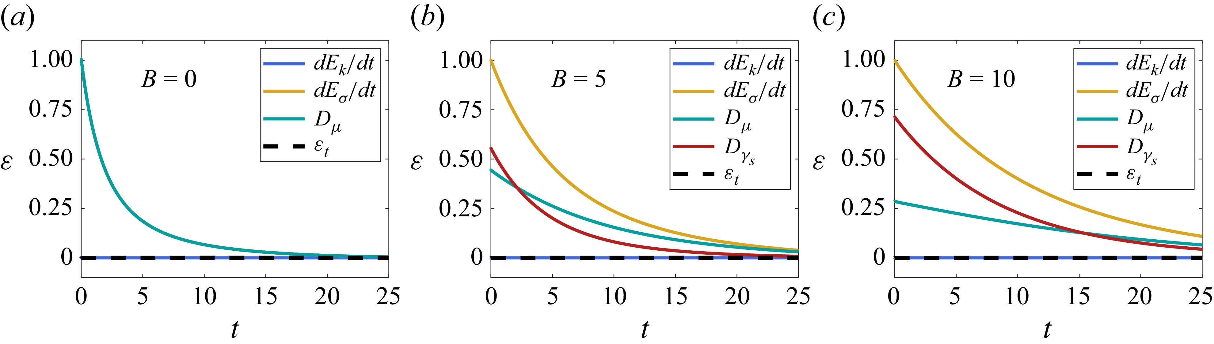
Computed evolution of one or more of the terms in (4.2), i.e. time rate of change of energy and/or dissipation, normalised by the rate of change of surface potential energy at $t=0$
,
$t=0$
, $\mathcal{E}$
: rate of change of kinetic energy
$\mathcal{E}$
: rate of change of kinetic energy ${\rm d} E_k/{\rm d}t$
(blue line), rate of change of surface potential energy
${\rm d} E_k/{\rm d}t$
(blue line), rate of change of surface potential energy ${\rm d} E_\sigma /{\rm d}t$
(yellow line), rate of energy dissipation due to bulk viscous stresses
${\rm d} E_\sigma /{\rm d}t$
(yellow line), rate of energy dissipation due to bulk viscous stresses $D_\mu$
(teal line) and that due to surface viscous stresses
$D_\mu$
(teal line) and that due to surface viscous stresses $D_{\gamma _s}$
(maroon line), and rate of change of total energy or
$D_{\gamma _s}$
(maroon line), and rate of change of total energy or $\mathcal{E}_t = {\rm d} E_k/{\rm d}t + {\rm d} E_\sigma /{\rm d}t + D_\mu + D_{\gamma _s}$
(dotted black line). Here,
$\mathcal{E}_t = {\rm d} E_k/{\rm d}t + {\rm d} E_\sigma /{\rm d}t + D_\mu + D_{\gamma _s}$
(dotted black line). Here, $L_0=50$
and
$L_0=50$
and $\textit{Oh}=1000$
.
$\textit{Oh}=1000$
.

Figure 3(a) shows that for a highly viscous sheet in the absence of surface viscous effects, the time rate of change of surface potential energy virtually equals the rate of energy dissipation owing to bulk viscous effects (the curves corresponding to ${\rm d} E_\sigma /{\rm d}t$
and
${\rm d} E_\sigma /{\rm d}t$
and $D_\mu$
overlap). However, figures 3(b) and 3(c) show that in the presence of surface viscous effects, the dissipation rate due to surface effects dominates that due to bulk viscous effects at early times, but the former becomes less important than the latter at late times. A scaling estimate of the time when dissipation rate owing to surface viscous effects and that due to bulk viscous effects become comparable can be obtained from the integrals for
$D_\mu$
overlap). However, figures 3(b) and 3(c) show that in the presence of surface viscous effects, the dissipation rate due to surface effects dominates that due to bulk viscous effects at early times, but the former becomes less important than the latter at late times. A scaling estimate of the time when dissipation rate owing to surface viscous effects and that due to bulk viscous effects become comparable can be obtained from the integrals for $D_{\gamma _s}$
and
$D_{\gamma _s}$
and $D_\mu$
as
$D_\mu$
as $D_{\gamma _s}/D_\mu \sim {B}/4h_m$
. Thus, the two types of dissipation rates become comparable when
$D_{\gamma _s}/D_\mu \sim {B}/4h_m$
. Thus, the two types of dissipation rates become comparable when $h_m \sim {B}/4$
. Hence, when
$h_m \sim {B}/4$
. Hence, when ${B} \gtrsim 4$
, dissipation rate due to surface viscous effects dominates that due to bulk viscous effects at early times, in accord with the simulation results shown in figure 3(b,c). The cross-over time
${B} \gtrsim 4$
, dissipation rate due to surface viscous effects dominates that due to bulk viscous effects at early times, in accord with the simulation results shown in figure 3(b,c). The cross-over time $t_{\text{co}}$
can be estimated by equating the two-term approximation for
$t_{\text{co}}$
can be estimated by equating the two-term approximation for $h_m$
from (3.7) and the cross-over value of
$h_m$
from (3.7) and the cross-over value of $h_m$
obtained previously, thereby yielding
$h_m$
obtained previously, thereby yielding $t_{\text{co}} \approx ({B}^2-16)/4$
. Therefore,
$t_{\text{co}} \approx ({B}^2-16)/4$
. Therefore, $t_{\text{co}} \approx 2$
when
$t_{\text{co}} \approx 2$
when ${B}=5$
, but
${B}=5$
, but $t_{\text{co}} \approx 21$
when
$t_{\text{co}} \approx 21$
when ${B}=10$
. The decreasing importance of surface viscous dissipation rate as time increases can also be appreciated by noting that since surface area
${B}=10$
. The decreasing importance of surface viscous dissipation rate as time increases can also be appreciated by noting that since surface area $A_s$
scales as
$A_s$
scales as $L$
and volume
$L$
and volume $V \sim L h_m$
, surface area to volume ratio,
$V \sim L h_m$
, surface area to volume ratio, $A_s/V \sim 1/h_m$
, falls as time increases and hence
$A_s/V \sim 1/h_m$
, falls as time increases and hence $h_m$
rises. Thus, surface viscous effects slow down the rate of retraction for the most part by slowing down the rate of growth of sheet thickness at early times.
$h_m$
rises. Thus, surface viscous effects slow down the rate of retraction for the most part by slowing down the rate of growth of sheet thickness at early times.
By incorporating the effect of intrinsic surface viscous forces into the slender-sheet equations, we have shown that surface viscosity slows the retraction of highly viscous Newtonian sheets. The reduced recoil rate due to surface viscosity has implications for situations where sheets disintegrate to form drops and others where sheet integrity and reduction of sheet shrinkage are crucial. Measured values of surface viscosity $\gamma _s$
lie in the range
$\gamma _s$
lie in the range $10^{-8}$
–
$10^{-8}$
– $10^{-4}\,{\rm Pa\,m\,s}$
(Stevenson Reference Stevenson2005). For a glycerol–water mixture of
$10^{-4}\,{\rm Pa\,m\,s}$
(Stevenson Reference Stevenson2005). For a glycerol–water mixture of $\rho \approx 1000\,{\rm kg\,m^{-3}}$
,
$\rho \approx 1000\,{\rm kg\,m^{-3}}$
, $\mu \approx 1\,{\rm Pa\,s}$
and
$\mu \approx 1\,{\rm Pa\,s}$
and $\sigma \approx 0.05\,{\rm N\,m^{-1}}$
(Liao, Franses & Basaran Reference Liao, Franses and Basaran2006), and
$\sigma \approx 0.05\,{\rm N\,m^{-1}}$
(Liao, Franses & Basaran Reference Liao, Franses and Basaran2006), and $\gamma _s \approx 10^{-5}\,{\rm Pa\,m\,s}$
,
$\gamma _s \approx 10^{-5}\,{\rm Pa\,m\,s}$
, $\textit{Oh} \approx 100$
and
$\textit{Oh} \approx 100$
and ${B} \approx 5$
for a film of
${B} \approx 5$
for a film of $\tilde {h}_0 \approx 2\,\rm \mu {m}$
(a value typical in many coating flows (Kistler & Scriven Reference Kistler and Scriven1983)). These values of
$\tilde {h}_0 \approx 2\,\rm \mu {m}$
(a value typical in many coating flows (Kistler & Scriven Reference Kistler and Scriven1983)). These values of $\textit{Oh}$
and
$\textit{Oh}$
and ${B}$
would place such a system well within the range of parameters for which predictions have been reported in this paper.
${B}$
would place such a system well within the range of parameters for which predictions have been reported in this paper.
Although surface viscosities were treated as constants in this work, the results are nevertheless broadly relevant to systems containing surfactant and polymer additives, but which exhibit constant surface viscosities (Manikantan & Squires Reference Manikantan and Squires2020; Herrada et al. Reference Herrada, Ponce-Torres, Rubio, Eggers and Montanero2022). Noteworthy extensions of this work include analysis of situations where it may be possible to derive the counterpart of (3.5) when surface viscosities are not constants and depend, for example, on surfactant concentration. As surface viscosities enter the planar problem studied here as $\gamma _s^s + \gamma _s^d$
as opposed to
$\gamma _s^s + \gamma _s^d$
as opposed to $({9}/{2}) \gamma _s^s + ({1}/{2}) \gamma _s^d$
in problems involving cylindrical filaments and jets (Wee et al. Reference Wee, Wagoner, Kamat and Basaran2020, Reference Wee, Wagoner and Basaran2022a
, Reference Wee, Kumar, Dhanwani and Basaran2024a
), experiments in planar and cylindrical geometries can be used in tandem to infer the individual values of the two surface viscosities. Surface phases can also be non-Newtonian (Fuller & Vermant Reference Fuller and Vermant2012; Underhill, Hirsa & Lopez Reference Underhill, Hirsa and Lopez2017; Wee et al. Reference Wee, Kumar, Dhanwani and Basaran2024a
). An open question is whether viscoelastic surface rheology, as bulk viscoelastic rheology (Sen et al. Reference Sen, Datt, Segers, Wijshoff, Snoeijer, Versluis and Lohse2021), can speed up recoil of liquid sheets.
$({9}/{2}) \gamma _s^s + ({1}/{2}) \gamma _s^d$
in problems involving cylindrical filaments and jets (Wee et al. Reference Wee, Wagoner, Kamat and Basaran2020, Reference Wee, Wagoner and Basaran2022a
, Reference Wee, Kumar, Dhanwani and Basaran2024a
), experiments in planar and cylindrical geometries can be used in tandem to infer the individual values of the two surface viscosities. Surface phases can also be non-Newtonian (Fuller & Vermant Reference Fuller and Vermant2012; Underhill, Hirsa & Lopez Reference Underhill, Hirsa and Lopez2017; Wee et al. Reference Wee, Kumar, Dhanwani and Basaran2024a
). An open question is whether viscoelastic surface rheology, as bulk viscoelastic rheology (Sen et al. Reference Sen, Datt, Segers, Wijshoff, Snoeijer, Versluis and Lohse2021), can speed up recoil of liquid sheets.
Funding
The authors thank the Purdue Process Safety and Assurance Center (P2SAC) for financial support.
Declaration of interests
The authors report no conflict of interest.
Appendix. 2-D simulations
In this appendix, we provide an overview of the fully 2-D Navier–Stokes solver that we have used, and which is described in great detail in numerous publications dating back more than twenty years (see, e.g. Notz & Basaran Reference Notz and Basaran2004, Anthony et al. Reference Anthony2023). We also compare at finite Ohnesorge numbers computational results obtained from 1-D simulations, the approach adopted in the main body of this paper, with those obtained from 2-D simulations using this solver which does not invoke the slenderness approximation.
Sheet retraction is a transient free boundary problem governed by the 2-D continuity and Navier–Stokes equations. As in the 1-D formulation, we exploit symmetry and solve only the problem over one quarter of the domain. On the free surface, we impose the kinematic boundary condition and the traction boundary condition (2.1). The governing equations are solved numerically using a fully implicit, sharp-interface arbitrary Lagrangian–Eulerian method-of-lines algorithm, in which the Galerkin finite-element method (G/FEM) is used for spatial discretisation and an adaptive implicit finite-difference scheme is employed for time integration (Anthony et al. Reference Anthony2023; Wee et al. Reference Wee, Kumar, Liu and Basaran2024b ). Since the problem involves a free surface, elliptic mesh generation (Christodoulou & Scriven Reference Christodoulou and Scriven1992) is used to track the interface profile and to determine the coordinates of each grid point in the moving, adaptive mesh simultaneously with the velocity and pressure fields in the sheet. As modelling flows with surface rheology is challenging, only a limited number of numerical methods have been developed to address these types of situations. Examples of such methods include the boundary element or integral method (BEM/BIM), which has been used by Singh & Narsimhan (Reference Singh and Narsimhan2022) to model surface rheological effects in breakup of drops undergoing Stokes flow, spectral methods to model interface pinch-off (Ponce-Torres et al. Reference Ponce-Torres, Rubio, Herrada, Eggers and Montanero2020), and finite-Reynolds-number, sharp interface methods like the one described in this appendix to simulate the breakup of liquid jets and sheets (Wee et al. Reference Wee, Wagoner, Garg, Kamat and Basaran2021, Reference Wee, Kumar, Dhanwani and Basaran2024a ; Cunha, Ribeiro & Carvalho Reference Cunha, Ribeiro and Carvalho2023).
Variation in time of the maximum film half-thickness $h_m=h(z=0,t)$
when (a)
$h_m=h(z=0,t)$
when (a) ${B}=0$
and (b)
${B}=0$
and (b) ${B}=10$
obtained from 1-D (open circle symbols) and 2-D (open square symbols) numerical simulations, and analytically (dimensionless form of (1.1) (panel a) and (3.5) (panel b), both denoted by black lines). Here, blue symbols correspond to
${B}=10$
obtained from 1-D (open circle symbols) and 2-D (open square symbols) numerical simulations, and analytically (dimensionless form of (1.1) (panel a) and (3.5) (panel b), both denoted by black lines). Here, blue symbols correspond to $\textit{Oh}=1000$
, teal symbols to
$\textit{Oh}=1000$
, teal symbols to $\textit{Oh}=100$
, yellow symbols to
$\textit{Oh}=100$
, yellow symbols to $\textit{Oh}=10$
and maroon symbols to
$\textit{Oh}=10$
and maroon symbols to $\textit{Oh}=1$
. The data points corresponding to
$\textit{Oh}=1$
. The data points corresponding to $\textit{Oh}=1000$
and
$\textit{Oh}=1000$
and $\textit{Oh}=100$
lie on top of one another, demonstrating excellent agreement between the non-inertial theory and simulations when
$\textit{Oh}=100$
lie on top of one another, demonstrating excellent agreement between the non-inertial theory and simulations when $\textit{Oh}(1+{B})$
is large. In the simulations,
$\textit{Oh}(1+{B})$
is large. In the simulations, $L_0=50$
.
$L_0=50$
.

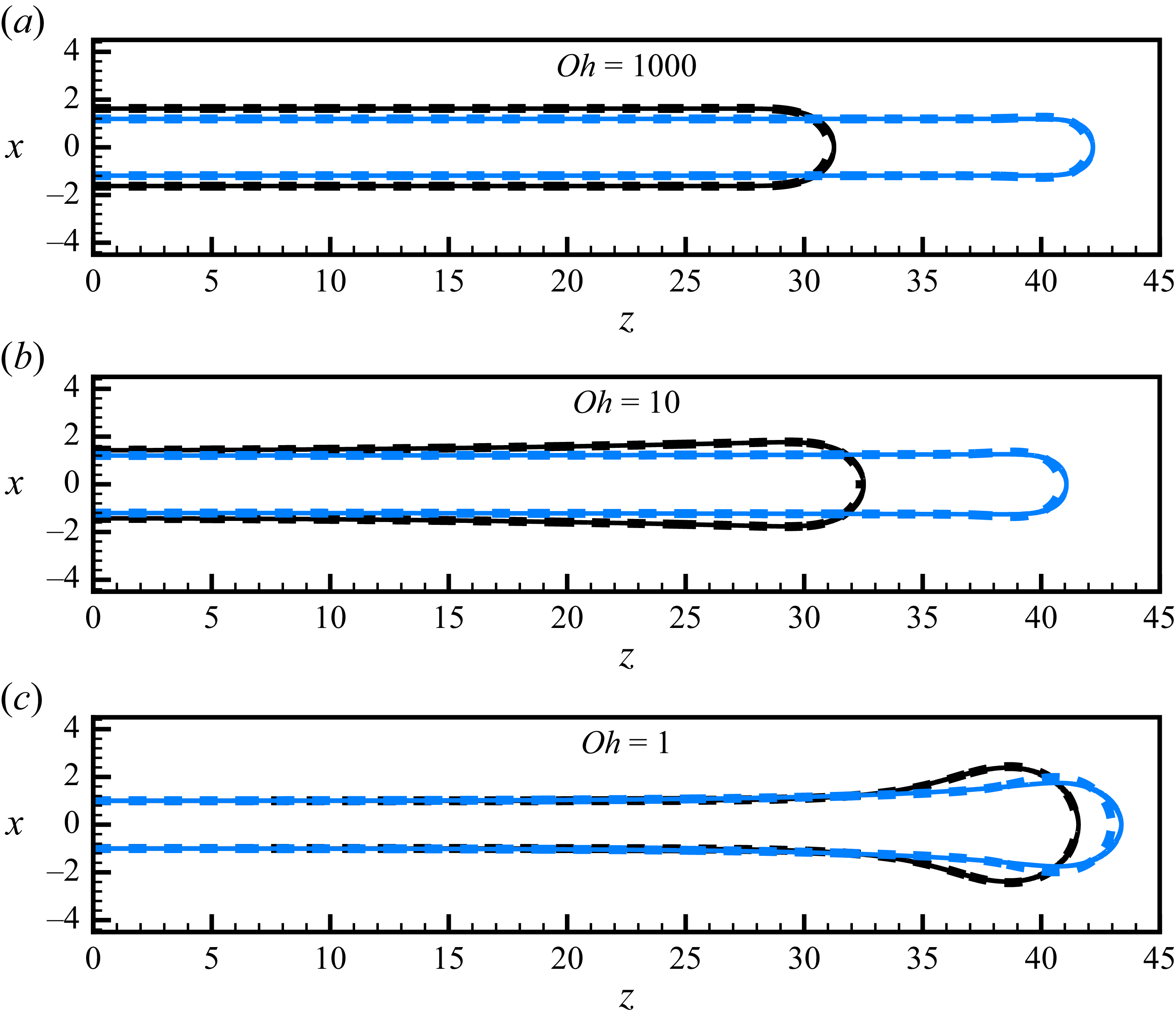
Comparison of the instantaneous shapes of retracting sheets obtained from 1-D (solid lines) and 2-D (dashed lines) numerical simulations at different $\textit{Oh}$
when
$\textit{Oh}$
when ${B}=0$
(black lines) and
${B}=0$
(black lines) and ${B}=10$
(blue lines). Shape profiles for sheets of (a)
${B}=10$
(blue lines). Shape profiles for sheets of (a) $\textit{Oh}=1000$
at
$\textit{Oh}=1000$
at $t\approx 2.5$
; (b)
$t\approx 2.5$
; (b) $\textit{Oh}=10$
at
$\textit{Oh}=10$
at $t \approx 3.4$
; and (c)
$t \approx 3.4$
; and (c) $\textit{Oh}=1$
at
$\textit{Oh}=1$
at $t \approx 12$
. Here,
$t \approx 12$
. Here, $L_0=50$
.
$L_0=50$
.

As discussed in the works of Brenner & Gueyffier (Reference Brenner and Gueyffier1999) and, more recently, Deka & Pierson (Reference Deka and Pierson2020), a retracting viscous sheet may develop a rim even when $\textit{Oh}$
is large. These studies have shown that a rim does not form and the sheet remains nearly flat provided that
$\textit{Oh}$
is large. These studies have shown that a rim does not form and the sheet remains nearly flat provided that $L_0 \ll \textit{Oh}$
. In the presence of surface rheological effects, a simple scaling analysis reveals that rims do not form if
$L_0 \ll \textit{Oh}$
. In the presence of surface rheological effects, a simple scaling analysis reveals that rims do not form if $\textit{Oh}\,(1+{B}) \gg L_0$
. Accordingly, we focus in the present work on this regime in which the sheet remains essentially flat and the theory that is based on Stokes flow applies.
$\textit{Oh}\,(1+{B}) \gg L_0$
. Accordingly, we focus in the present work on this regime in which the sheet remains essentially flat and the theory that is based on Stokes flow applies.
Figure 4 shows the evolution in time of $h_m$
and figure 5 shows instantaneous shapes of retracting sheets obtained from 1-D and 2-D simulations at several
$h_m$
and figure 5 shows instantaneous shapes of retracting sheets obtained from 1-D and 2-D simulations at several $\textit{Oh}$
when surface rheological effects are absent and present. First, these figures demonstrate that the results obtained from 1-D simulations are in excellent agreement with those obtained from 2-D simulations. Figure 4 further demonstrates that when
$\textit{Oh}$
when surface rheological effects are absent and present. First, these figures demonstrate that the results obtained from 1-D simulations are in excellent agreement with those obtained from 2-D simulations. Figure 4 further demonstrates that when $\textit{Oh}\,(1+{B}) \gg L_0$
, the predictions made with the theory developed in this paper are in exellent agreement with simulations. When
$\textit{Oh}\,(1+{B}) \gg L_0$
, the predictions made with the theory developed in this paper are in exellent agreement with simulations. When ${B}=0$
, the absence or presence of rims as highlighted by the transient interface shape profiles shown in figure 5 also accords with results reported by Brenner & Gueyffier (Reference Brenner and Gueyffier1999), Savva & Bush (Reference Savva and Bush2009), Deka & Pierson (Reference Deka and Pierson2020) and Sanjay et al. (Reference Sanjay, Sen, Kant and Lohse2022) who studied retraction in the absence of surface rheological effects. As
${B}=0$
, the absence or presence of rims as highlighted by the transient interface shape profiles shown in figure 5 also accords with results reported by Brenner & Gueyffier (Reference Brenner and Gueyffier1999), Savva & Bush (Reference Savva and Bush2009), Deka & Pierson (Reference Deka and Pierson2020) and Sanjay et al. (Reference Sanjay, Sen, Kant and Lohse2022) who studied retraction in the absence of surface rheological effects. As $\textit{Oh}\,(1+{B})/L_0$
decreases, the onset of rim formation becomes increasingly evident. In this regime, inertial effects can no longer be neglected: motion driven by surface tension is resisted by inertia, leading to mass accumulation near the retracting tip. Together, figures 4 and 5 help delineate the parameter range over which the present non-inertial theory remains valid and indicate where deviations from that theory can be expected as inertial effects become significant.
$\textit{Oh}\,(1+{B})/L_0$
decreases, the onset of rim formation becomes increasingly evident. In this regime, inertial effects can no longer be neglected: motion driven by surface tension is resisted by inertia, leading to mass accumulation near the retracting tip. Together, figures 4 and 5 help delineate the parameter range over which the present non-inertial theory remains valid and indicate where deviations from that theory can be expected as inertial effects become significant.


 Open access