

INTRODUCTION
Precipitation, a major forcing of the hydrological cycle, is key to understanding past environments. As direct measurements are unavailable prior to modern instrumentation, calibrated proxy records sensitive to precipitation, primarily mean annual precipitation (MAP), can fill this need. Direct relationships or transfer functions from proxies to precipitation are hard to establish, however, and past conditions are often only qualitatively characterized. Consequently, qualitative terms such as drier/wetter conditions are adopted. Natural variance further complicates identification of distinct precipitation regimes and their temporal variability. For example, interannual variability and random clustering of dry and wet years can produce seemingly “natural” fluctuations that must be distinguished from true changes in precipitation regime or even climate change. An example of this is the discussion by Roe (Reference Roe2011) and Anderson et al. (Reference Anderson, Roe and Anderson2014) on glacier responses to climate change and their variability.
This paper focuses on the late Holocene in the Levant–eastern Mediterranean, a region with a rich history of human societies. It uses the reconstructed Dead Sea levels as a proxy for a precipitation regime in the Levant. A stochastic framework is applied that includes modeling of precipitation series and a water-balance model based on instrumentally recorded precipitation in the watershed of the Dead Sea and contemporaneous changes in the Dead Sea level. The proposed novel framework provides a rigorous and realistic quantitative assessment of reconstructed mean, variance, and trends of regional annual precipitation and their changes over the past 4500 yr.
The Dead Sea and its watershed
The Dead Sea is a hypersaline terminal lake (e.g., Neev and Emery, Reference Neev and Emery1967) located within a large morpho-tectonic depression along the Dead Sea transform (e.g., Garfunkel, Reference Garfunkel1981). It is the lowermost surface on continental Earth. In 2016, its water surface level was at an elevation of ~430 meters below sea level (m below sea level [bsl]). The Dead Sea is the name of the Holocene and modern lake, which is the last in a series of water bodies that filled this depression to different elevations during the Quaternary (e.g., Stein, Reference Stein2001). The lake has one of the largest watersheds in the Levant (~43,000 km2), draining the sub-humid (>800 mm/yr) Mediterranean zone in the north to hyperarid (<100 mm/yr) areas in the southern Negev and Sinai (Fig. 1). The lake itself is under hyperarid conditions, with MAP ranging from 70 to 45 mm/yr at the northern and southern ends of the lake, respectively. Precipitation occurs in the watershed in October–May (mostly in December–February). In the northern, wetter part of the watershed, precipitation is delivered by mid-latitude cyclones and is characterized by relatively high spatial correlation and a regional synchroneity of annual precipitation (Enzel et al., Reference Enzel, Bookman (Ken Tor), Sharon, Gvirtzman, Dayan, Ziv and Stein2003). The upper Jordan and Yarmouk Rivers (Fig. 1) drain this region through the Lower Jordan River into the Dead Sea and are responsible for most of the inflow into the lake under natural conditions (Gavrieli and Oren, Reference Gavrieli and Oren2004). Therefore, the lake levels, before the major water diversion of the 1960s, were well-correlated with precipitation at its northern watershed and thus make excellent proxies for past Levant precipitation (Klein and Flohn, Reference Klein and Flohn1987; Enzel et al., Reference Enzel, Bookman (Ken Tor), Sharon, Gvirtzman, Dayan, Ziv and Stein2003; Bookman et al., Reference Bookman, Enzel, Agnon and Stein2004; Torfstein et al., Reference Torfstein, Goldstein, Stein and Enzel2013). Current lake evaporation ranges from approximately 1100–1200 mm/yr and evaporation rate is negatively correlated with lake salinity (Lensky et al., Reference Lensky, Dvorkin, Lyakhovsky, Gertman and Gavrieli2005).
The Dead Sea and its watershed. Contours show present-day mean annual precipitation (mm). Triangles mark the four rain stations analyzed: (1) Kfar Giladi, (2) Deganya, (3) Nazareth, and (4) Jerusalem (Table 1).
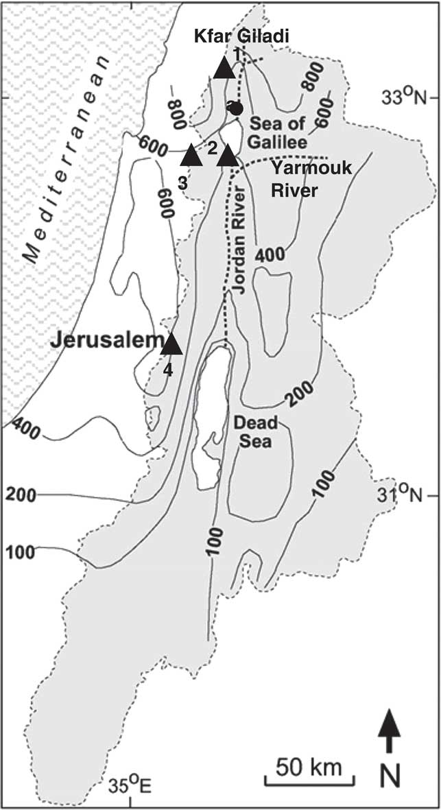
The Dead Sea is approximately 80 km long and <15 km wide, consisting of two sub-basins separated by a topographic sill at an elevation of ~402–403 m bsl (e.g., Bookman et al., Reference Bookman, Enzel, Agnon and Stein2004). At the beginning of the twentieth century, these two sub-basins were connected into one lake. The separation occurred in the late 1970s, following major water diversions from the Dead Sea watershed, which began in the 1960s. The northern basin is ~300 m deep and occupies more than two-thirds of the Dead Sea surface area (~650 km2). In contrast, the southern basin is relatively shallow (<10 m deep) and, without the presence of evaporation ponds used for potash extraction, would currently be dry. Under natural conditions, the sill served as a buffer for level changes (e.g., Enzel et al., Reference Enzel, Bookman (Ken Tor), Sharon, Gvirtzman, Dayan, Ziv and Stein2003); during lake-level rise, the southern basin was flooded and acted as an additional evaporation surface that limited additional rising. When the lake level declined below the sill elevation, the lake was confined to the northern basin, evaporation area decreased, and, therefore, the natural level decline slowed down. Intensive water diversions from the Dead Sea watershed have caused its dramatic level decline (currently >1 m/yr) since 1970. Furthermore, since the separation of the two basins, Dead Sea brine is pumped from the northern basin to the shallow southern basin, which acts as a huge evaporation pond that enables rapid salt precipitation and mining.
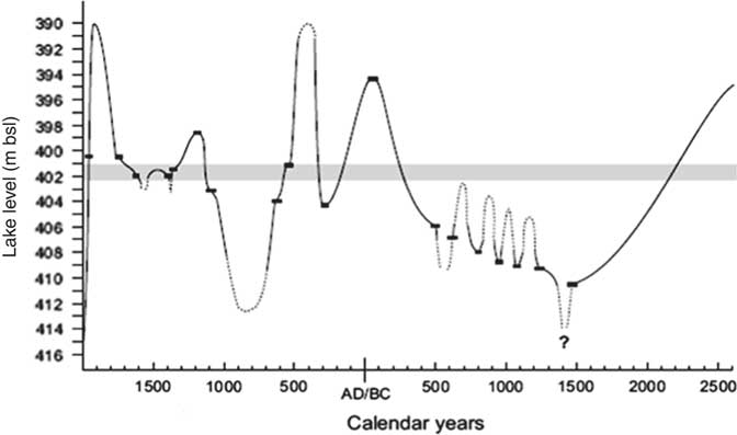
Due to the dramatic lake-level decline (>30 m since the 1970s), detailed Holocene stratigraphic records have become exposed along the Dead Sea (Kadan, Reference Kadan1996; Enzel et al., Reference Enzel, Kadan and Eyal2000; Bartov et al., Reference Bartov, Stein, Enzel, Agnon and Reches2002). Based on radiocarbon ages from exposures such as buried shoreline and beach deposits, which are direct indicators of lake levels, Bookman et al. (Reference Bookman, Enzel, Agnon and Stein2004) derived a late Holocene lake-level curve for the Dead Sea (Fig. 2). The lake-level curve for the early and middle Holocene (4000–8000 yr BP) is less complete than for the late Holocene, as it is based on only a small number of high-quality high-stand indicators (Frumkin et al., Reference Frumkin, Magaritz, Zak and Carmi1991; Kadan, Reference Kadan1996; Migowski et al., Reference Migowski, Stein, Prasad, Negendank and Agnon2006; Frumkin et al., Reference Frumkin, Bar-Yosef and Schwarcz2011; Kagan et al., Reference Kagan, Langgut, Boaretto, Neumann and Stein2015).
Reconstructed Dead Sea level (after Bookman et al., Reference Bookman, Enzel, Agnon and Stein2004); sill level is shown as a thick gray line.

Precipitation-lake-level relationships
Only a few studies have attempted to define the relationships between Dead Sea level fluctuations and precipitation in the lake's watershed (Rosenan, Reference Rosenan1959; Klein and Flohn, Reference Klein and Flohn1987; Enzel et al., Reference Enzel, Bookman (Ken Tor), Sharon, Gvirtzman, Dayan, Ziv and Stein2003; Kushnir and Stein, Reference Kushnir and Stein2010). Enzel et al. (Reference Enzel, Bookman (Ken Tor), Sharon, Gvirtzman, Dayan, Ziv and Stein2003) defined a relationship between changing lake levels and annual precipitation in Jerusalem for 1870–1960, extracting ≥4-yr-long sections from the modern level curve of net declining, rising, and stable levels, and correlating them to the mean coeval annual precipitation. That study, with its simple deterministic approach, proposed that multiyear lake-level rises and declines are associated with ±20% deviation from modern MAP, equal to 80% of the MAP's standard deviation. It provided some quantitative information on the magnitude of the precipitation fluctuations required for lake-level changes, which lasted ≥4 yr; however, the extraction of quantitative estimations of past precipitation regime in the Levant remains a challenge. Moreover, as shown by Enzel et al. (Reference Enzel, Bookman (Ken Tor), Sharon, Gvirtzman, Dayan, Ziv and Stein2003), attributing lake-level rises and declines to changes in precipitation regime should separate the effects of natural precipitation variability and precipitation trends. This is a challenge in paleoclimatology, even when transforming a record that has been shown to be derived from precipitation to a measurable proxy.
Lake-balance models for paleohydrologic studies
Lake-balance models are often used as a tool for reconstructing past climatic and hydrological conditions from lake proxy records. Most models are based on mass balance of water, chemical or isotopic composition, or energy balance (e.g., Cross et al., Reference Cross, Baker, Seltzer, Fritz and Dunbar2001; Rowe and Dunbar, Reference Rowe and Dunbar2004; Lensky et al., Reference Lensky, Dvorkin, Lyakhovsky, Gertman and Gavrieli2005; Shanahan et al., Reference Shanahan, Overpeck, Sharp, Scholz and Arko2007; Placzek et al., Reference Placzek, Quade and Patchett2013; Rosenmeier et al., Reference Rosenmeier, Brenner, Hodell, Martin, Curtis and Binford2016). Obviously, a large range of processes with complex interactions determine the above fluxes, and their modeling requires enormous amounts of data, which are usually unavailable, especially for paleohydrologic simulations. Therefore, most lake models substantially simplify the system representation to better accommodate the limited available knowledge and data.
Water-balance models for terminal lakes commonly consider fluxes into the lake by estimating watershed (not including lake area) precipitation minus evapotranspiration and direct lake precipitation, whereas outflow flux is represented by evaporation from the lake surface area (e.g., Rowe and Dunbar, Reference Rowe and Dunbar2004). Lake evaporation, being a major component in the balance, is estimated with a range of methodologies and semi-empirical formulas that involve different meteorological inputs, including short- and long-wave radiation fluxes, albedo, wind speed, relative humidity, air temperature, lake surface temperature, and others (Cross et al., Reference Cross, Baker, Seltzer, Fritz and Dunbar2001; Winter et al., Reference Winter, Buso, Rosenberry, Likens, Sturrock and Mau2003; Rosenberry et al., Reference Rosenberry, Winter, Buso and Likens2007; Placzek et al., Reference Placzek, Quade and Patchett2013 and references therein). For saline lakes, such as the Dead Sea, a very important factor affecting evaporation rate is water salinity or density, since the dissolved salts lower the saturation vapor pressure above the lake surface; consequently, the evaporation rates are lower compared to fresh water under similar conditions (Stanhill, Reference Stanhill1994; Yechieli and Gavrieli, Reference Yechieli, Gavrieli, Berkowitz and Ronen1998; Lensky et al., Reference Lensky, Dvorkin, Lyakhovsky, Gertman and Gavrieli2005; Hamdani et al., Reference Hamdani, Assouline, Tanny, Lensky, Gertman, Mor and Lensky2018; Mor et al., Reference Mor, Assouline, Tanny, Lensky and Lensky2018).
The present paper is aimed at quantitatively assessing precipitation regime in the Levant during the late Holocene while considering natural interannual precipitation variability. We confront this challenge by utilizing a stochastic framework and a water-balance model to link precipitation and Dead Sea levels. The water-balance model and its application to the Dead Sea are presented in the Modeling Lake-Level Change in Response to Precipitation Change. We then present utilization of the model in a stochastic framework to assess the probability of precipitation scenarios and reconstruction of the late Holocene precipitation regime. Discussion and concluding remarks are provided in the last two sections.
MODELING LAKE-LEVEL CHANGE IN RESPONSE TO PRECIPITATION CHANGE
A water-balance model was developed as the main tool to relate annual precipitation over the Dead Sea watershed and lake levels. The modeling approach used in this study keeps annual precipitation as the only time-varying input variable, while other variables affecting lake levels are either estimated from the model state variables or their effect is bulked within an uncertainty range around the model estimation. As explained below, some simplified, but justified, assumptions underlie the model's formulation and contribute to its robustness and its flexible utilization for non-instrumented periods.
The model input is a time series of annual precipitation depth P
1
…P
N
(a year is considered from October 1 to September 30); the initial condition is lake level at the beginning of the first year of computation, L
1
, and its output is a series of lake levels at the beginning of each year starting from the second, $L_{2} \,\cdots\,L_{{N{\plus}1}} $
. The model is based on the following steps applied for each year, t: (1) the volume of water at the lake at the beginning of the year is computed from the level at this time,
$L_{2} \,\cdots\,L_{{N{\plus}1}} $
. The model is based on the following steps applied for each year, t: (1) the volume of water at the lake at the beginning of the year is computed from the level at this time, $L_{t} ,$
using the lake-level-volume relationship; (2) the volume of water entering the lake,
$L_{t} ,$
using the lake-level-volume relationship; (2) the volume of water entering the lake, $Vin_{t} $
, is computed as a function of the annual precipitation and added to the lake volume; (3) the volume of water leaving the lake by evaporation,
$Vin_{t} $
, is computed as a function of the annual precipitation and added to the lake volume; (3) the volume of water leaving the lake by evaporation, $Vout_{t} $
, is computed using the lake-level water-density-evaporation rate relationship and lake surface area (derived from its level) and subtracted from the lake volume; (4) the lake level at the beginning of the following year,
$Vout_{t} $
, is computed using the lake-level water-density-evaporation rate relationship and lake surface area (derived from its level) and subtracted from the lake volume; (4) the lake level at the beginning of the following year, $L_{{t{\plus}1}} $
, is computed from the updated lake volume using the lake-level-volume relationship. The relationships among lake level, volume, and surface area were derived based on lake bathymetry data (Hall, Reference Hall1997) by applying GIS procedures.
$L_{{t{\plus}1}} $
, is computed from the updated lake volume using the lake-level-volume relationship. The relationships among lake level, volume, and surface area were derived based on lake bathymetry data (Hall, Reference Hall1997) by applying GIS procedures.
Estimation of annual water volume leaving the lake
The annual volume of water leaving the lake, $Vout_{t} $
(m3/yr), is the annual lake evaporation rate multiplied by the lake surface area associated with the given lake level. Lake evaporation is a complex process and its rate depends on meteorological conditions of the surrounding environment and water-body conditions. Recent studies of the Dead Sea (Stanhill, Reference Stanhill1994; Lensky et al., Reference Lensky, Dvorkin, Lyakhovsky, Gertman and Gavrieli2005) have utilized energy- and mass-balance approaches and measurements from meteorological stations and lake sensors to estimate monthly and annual evaporation rates. Those studies showed a negative correlation between evaporation rate and salinity or density. For the current study, we aimed to obtain a simple but robust estimation of annual lake evaporation rate that can be extended to non-instrumented periods of the late Holocene, and therefore considered the relations among annual evaporation rate, water density, and lake levels. A decrease in lake evaporation rate was attributed to a reduction in fresh water entering the lake accompanied by an increase in lake salinity and density and a reduction in activity of the water in the solution (Stanhill, Reference Stanhill1994; Yechieli et al., 1998). Stanhill (Reference Stanhill1994) indicated that the relations between water density and evaporation rate are not simple and are affected by feedback mechanisms, which involve changes in the radiation balance, surface vapor pressure, and microclimate; strong empirical linear relations, however, were evident between the two variables. To examine and extract these empirical relationships, we constructed two data sets based on published information (Ashbel, Reference Ashbel1951; Neuman, Reference Neumann1958; Steinhorn et al., Reference Steinhorn, Assaf, Gat, Nishry, Nissenbaum, Stiller and Beyth1979; Beyth, Reference Beyth1980; Stanhill, Reference Stanhill1994; Yechieli et al., 1998; Lensky et al., Reference Lensky, Dvorkin, Lyakhovsky, Gertman and Gavrieli2005) and data from the Geological Survey of Israel, partly published in internal reports. The first data set included simultaneous lake-level and water-density measurements from 1936 to 2011 (Fig. 3a) and the second included estimation of annual evaporation rates using mass- or energy-balance methods and density data from 1936 to 2000 (Ashbel, Reference Ashbel1951; Neuman, Reference Neumann1958; Stanhill, Reference Stanhill1994; Lensky et al., Reference Lensky, Dvorkin, Lyakhovsky, Gertman and Gavrieli2005) and from simulations conducted for hypothetical cases (Fig. 3b; Yechieli et al., 1998).
$Vout_{t} $
(m3/yr), is the annual lake evaporation rate multiplied by the lake surface area associated with the given lake level. Lake evaporation is a complex process and its rate depends on meteorological conditions of the surrounding environment and water-body conditions. Recent studies of the Dead Sea (Stanhill, Reference Stanhill1994; Lensky et al., Reference Lensky, Dvorkin, Lyakhovsky, Gertman and Gavrieli2005) have utilized energy- and mass-balance approaches and measurements from meteorological stations and lake sensors to estimate monthly and annual evaporation rates. Those studies showed a negative correlation between evaporation rate and salinity or density. For the current study, we aimed to obtain a simple but robust estimation of annual lake evaporation rate that can be extended to non-instrumented periods of the late Holocene, and therefore considered the relations among annual evaporation rate, water density, and lake levels. A decrease in lake evaporation rate was attributed to a reduction in fresh water entering the lake accompanied by an increase in lake salinity and density and a reduction in activity of the water in the solution (Stanhill, Reference Stanhill1994; Yechieli et al., 1998). Stanhill (Reference Stanhill1994) indicated that the relations between water density and evaporation rate are not simple and are affected by feedback mechanisms, which involve changes in the radiation balance, surface vapor pressure, and microclimate; strong empirical linear relations, however, were evident between the two variables. To examine and extract these empirical relationships, we constructed two data sets based on published information (Ashbel, Reference Ashbel1951; Neuman, Reference Neumann1958; Steinhorn et al., Reference Steinhorn, Assaf, Gat, Nishry, Nissenbaum, Stiller and Beyth1979; Beyth, Reference Beyth1980; Stanhill, Reference Stanhill1994; Yechieli et al., 1998; Lensky et al., Reference Lensky, Dvorkin, Lyakhovsky, Gertman and Gavrieli2005) and data from the Geological Survey of Israel, partly published in internal reports. The first data set included simultaneous lake-level and water-density measurements from 1936 to 2011 (Fig. 3a) and the second included estimation of annual evaporation rates using mass- or energy-balance methods and density data from 1936 to 2000 (Ashbel, Reference Ashbel1951; Neuman, Reference Neumann1958; Stanhill, Reference Stanhill1994; Lensky et al., Reference Lensky, Dvorkin, Lyakhovsky, Gertman and Gavrieli2005) and from simulations conducted for hypothetical cases (Fig. 3b; Yechieli et al., 1998).
Empirical relationships between (a) lake level and water density, and (b) water density and evaporation rate. Equations 1 and 2 (see text) were fitted to the data, and 95% uncertainties (for an individual observation) were computed using the Matlab nlinfit and nlpredci tools. Data from Ashbel (Reference Ashbel1951), Neuman (1958), Steinhorn et al. (Reference Steinhorn, Assaf, Gat, Nishry, Nissenbaum, Stiller and Beyth1979), Beyth (Reference Beyth1980), Stanhill (Reference Stanhill1994), Yechieli et al. (1998), Oren, (2004), Lensky et al. (Reference Lensky, Dvorkin, Lyakhovsky, Gertman and Gavrieli2005). The fitted curve is shown in black lines, uncertainty range in gray lines and data in blue circles. Performance criteria, R 2, and root mean square difference (RMSD) are presented for each fitted function. (For interpretation of the references to color in this figure legend, the reader is referred to the web version of this article.)

Two empirical functions were fitted to the data: a spherical–linear function relating annual lake level $L_{t} $
(m bsl) and annual surface water density
$L_{t} $
(m bsl) and annual surface water density $\rho _{t} $
(g/cm3):
$\rho _{t} $
(g/cm3):
 $$\rho _{t} {\equals}\left\{ {\matrix{ {L_{t} \,\lt\,b_{3} } & {b_{1} {\plus}b_{2} {\times}\left( {1.5{\times}\left( {{{L_{t} } \over {b_{3} }}} \right){\minus}0.5{\times}\left( {{{L_{t} } \over {b_{3} }}} \right)^{3} } \right)} \cr {otherwise} & {b_{1} {\plus}b_{2} {\plus}b_{4} {\times}\left( {L_{t} {\minus}b_{3} } \right)} \cr } } \right\}$$
 The computed density cannot go below the freshwater value of 1 g/cm3. The function coefficients, determined using Matlab nlinfit tool, were: $b_{1} $
= −63.23 g/cm3,
$b_{1} $
= −63.23 g/cm3, $b_{2} $
= 64.5 g/cm3,
$b_{2} $
= 64.5 g/cm3, $b_{3} $
= 401.9 m bsl, and
$b_{3} $
= 401.9 m bsl, and $b_{4} $
= 0.00035 g/cm3/m. The first three coefficients determine the relatively rapid increase in water density as lake-level declines (i.e., L increases) up to 401.9 m bsl (
$b_{4} $
= 0.00035 g/cm3/m. The first three coefficients determine the relatively rapid increase in water density as lake-level declines (i.e., L increases) up to 401.9 m bsl ( $b_{3} $
), whereas a further reduction in lake level continues to increase water density but at a much lower rate (
$b_{3} $
), whereas a further reduction in lake level continues to increase water density but at a much lower rate ( $b_{4} $
).
$b_{4} $
).
A linear function relates annual surface water density, $\rho _{t} $
(g/cm3), and annual evaporation rate,
$\rho _{t} $
(g/cm3), and annual evaporation rate, $E_{t} $
(m/yr):
$E_{t} $
(m/yr):
 $$E_{t} {\equals}c_{1} {\times}\rho _{t} {\plus}c_{2} $$
 The coefficients of Eq. 2 are: $c_{1} $
= −4.72 (m*cm3)/yr/g and
$c_{1} $
= −4.72 (m*cm3)/yr/g and $c_{2} $
= 6.98 m/yr. Uncertainty bounds of 95% computed with the above fitting function for both equations are shown in Figure 3 together with performance criteria, R
2, and root mean square difference (RMSD).
$c_{2} $
= 6.98 m/yr. Uncertainty bounds of 95% computed with the above fitting function for both equations are shown in Figure 3 together with performance criteria, R
2, and root mean square difference (RMSD).
A few sources contribute to the uncertainty range of the density and evaporation rate estimation presented above. A major source is data uncertainty, which includes potential errors in measurements or in the estimated values that comprise the data sets, as well as representation issues (e.g., data from a given date and location do not necessarily represent the entire year and lake). Another source is variability in controlling factors that were not directly accounted for in the model, including meteorological conditions, lake-body conditions, and hysteresis in lake-level-density relations, the latter referring to a stratified versus homogeneous water column. During lake-level rise, the excess inflow versus evaporation leads to the development of a more dilute upper water body relative to the deeper, main brine body of the lake. Conversely, during lake-level decline, the excess evaporation results in increased density. As long as the lake is stratified, evaporation will occur solely from the upper water body. Overturn and water column homogenization will eventually take place when the density of the surface water reaches that of the lower brines. The lake level at which this occurs, however, is a function of the processes experienced by the lake since stratification last began and depends on the relative amounts of salt that have accumulated in the upper water and dilution of the lower brines, among other things (e.g., Torfstein et al., Reference Torfstein, Gavrieli and Stein2005). Thus, overturn may occur at water levels that differ from that at which stratification first developed.
It can be noted that uncertainties in evaporation rates with our method (Fig. 3b) are relatively large, ranging between ±17 and ±23% of the mean value for a density range of 1.1 to 1.25 g/cm. This is larger than reported, for example, by Lensky et al. (Reference Lensky, Dvorkin, Lyakhovsky, Gertman and Gavrieli2005) for the estimated Dead Sea evaporation rate for 1999 using the Bowen’s approach; they realized that uncertainties in several controlling factors, such as long-wave radiation, albedo, and lake temperature, result in a range of evaporation rates of 1.1–1.21 m/yr, i.e., ±5% of the mean value. Considering the complexity of the process and the simplified approach taken in our study, we consider the obtained uncertainty levels to be reasonable. Moreover, we utilize this range to further examine the propagation of these uncertainties in our model and quantify the uncertainty range of modeled lake levels.
An evaluation of the estimated $Vout_{t} $
, independent of the lake inflow estimation (described in the next section), is possible for 1991/1992, which was an exceptionally wet year in the study region. As mentioned earlier, since the 1970s, human intervention in the lake watershed has been substantial and lake level has fallen steeply. Due to the large precipitation amounts in 1991/1992, the lake inflow was high and the total annual volume of water entering the lake was estimated by Beyth et al. (Reference Beyth, Gavrieli, Anati and Katab1993) as 1.5 × 10⁹ m3/yr, raising the lake level by more than 2 m from 408.228 m bsl, the observed level at the beginning of the 1991 hydrological year. Applying the functional relations presented earlier to the 1991/1992 lake conditions, we estimate lake surface density as 1.2344 g/cm3 and an annual evaporation rate of 1.156 m/yr. The estimated lake level at the end of the year is 407.160 m bsl (407.390–406.922 m bsl representing the 95% uncertainty range), which compares well with the observed lake level of 407.204 m bsl on October 1, 1992.
$Vout_{t} $
, independent of the lake inflow estimation (described in the next section), is possible for 1991/1992, which was an exceptionally wet year in the study region. As mentioned earlier, since the 1970s, human intervention in the lake watershed has been substantial and lake level has fallen steeply. Due to the large precipitation amounts in 1991/1992, the lake inflow was high and the total annual volume of water entering the lake was estimated by Beyth et al. (Reference Beyth, Gavrieli, Anati and Katab1993) as 1.5 × 10⁹ m3/yr, raising the lake level by more than 2 m from 408.228 m bsl, the observed level at the beginning of the 1991 hydrological year. Applying the functional relations presented earlier to the 1991/1992 lake conditions, we estimate lake surface density as 1.2344 g/cm3 and an annual evaporation rate of 1.156 m/yr. The estimated lake level at the end of the year is 407.160 m bsl (407.390–406.922 m bsl representing the 95% uncertainty range), which compares well with the observed lake level of 407.204 m bsl on October 1, 1992.
The relationships found for the modern-day period to estimate evaporation rates are assumed to hold for the entire late Holocene. This extrapolation assumes that during the past 4500 yr, changes in lake evaporation controls were small compared to their variability in the present-day period, and on the uncertainty in the evaporation rate estimates (Fig. 3b). Only limited information is available on some of the important evaporation controls during the late Holocene. Temperature and relative humidity for different periods during the past 56,000 yr were estimated by Affek et al. (Reference Affek, Bar-Matthews, Ayalon, Matthews and Eiler2008) based on speleothem carbonates from the Soreq Cave in Israel. They found that, during the late Holocene (representing the past 2000 yr in their research), temperatures were slightly lower and relative humidity was similar to present-day climatic conditions. Changes in solar radiation, the largest component of the energy balance (Lensky et al., Reference Lensky, Dvorkin, Lyakhovsky, Gertman and Gavrieli2005), related to variations in orbital insolation were no more than 0.2% during the past 5000 yr (Berger and Loutre, Reference Berger and Loutre1991). This is much smaller than the 10% reduction in solar radiation reaching the lake in 1999 relative to the pre-1950 values (Lensky et al., Reference Lensky, Dvorkin, Lyakhovsky, Gertman and Gavrieli2005), presumably due to global dimming (Stanhill and Cohen, Reference Stanhill and Cohen2001). Given the above indications, considering the large uncertainties in Dead Sea evaporation rate estimates and based on our best judgement, use of the derived relationships presented in Equations 1 and 2 for the past 4500 yr is reasonable. In addition, we emphasize that the data sets used to derive those relationships represent a large range of conditions and lake levels (390–555 m bsl) and most importantly, they cover the entire range of lake levels obtained for the late Holocene (Fig. 2).
Estimation of annual water volume entering the lake
As explained earlier, we consider annual precipitation to be the main forcing of the model by controlling lake inflow. In the present section, we first determine which rain station best represents annual changes in lake level, then a linear model is set to compute annual lake inflow volume as a function of annual precipitation at the selected station; finally, the model is calibrated, validated, and the uncertainty range estimated. Model development is based on precipitation and lake-level data for the period 1930–1961, representing the interval for which systematic precipitation and lake-level data are available and human intervention in the system was minimal. The substantial lake-level decline resulting from the upstream water diversion from the Dead Sea watershed began subsequent to this interval, in the early 1970s.
Several rain stations (Kfar Giladi, Deganya, Nazareth, and Jerusalem; Fig. 1) located in the Dead Sea drainage watershed with data for the time interval of interest were considered. Linear correlations between annual precipitation measured at the stations and annual changes in lake level (i.e., the difference between lake levels at the end and beginning of each hydrological year) are shown in Table 1 (non-linear relationships were also examined but the general model performance was not improved). The highest R 2 value of a single station was for the Kfar Giladi annual precipitation data (Table 1); this station is located in the northern, wetter part of the watershed (Fig. 1) responsible for the largest contribution of inflow to the Dead Sea (via the Jordan River) under natural conditions. The inclusion of data from additional stations using a multiple-regression framework, somewhat improved R 2 (Table 1). Due to the typical high interstation correlation of annual precipitation (Table 2), however, model performance was not improved (i.e., if precipitation input is taken as a weighted sum of the data from two or more stations, the minimal model error is obtained when the entire weight is put on one of the stations). Therefore, we chose to base the model on the Kfar Giladi data alone, rather than combining them with data from any other station.
Correlation of annual precipitation and lake level change for the period 1930-1961.

Correlation of annual precipitation in Kfar Giladi station and other stations for the period 1930–1961.

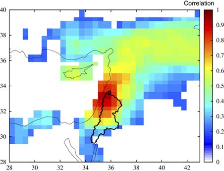
Relationships between precipitation over the lake watershed and volume of water entering the lake are expected to be quite complex due to heterogeneity of watershed properties and precipitation patterns. We claim that, on an annual scale, however, a simplified linear relation between Kfar Giladi precipitation and lake inflow is sufficiently good for the following reasons: (1) annual precipitation over the area contributing most of the inflow to the Dead Sea presents spatial synchronization (Enzel et al., Reference Enzel, Bookman (Ken Tor), Sharon, Gvirtzman, Dayan, Ziv and Stein2003). This is manifested in the relatively high correlations of annual precipitation data from the Kfar Giladi station with other stations in the region (Table 2) or with data from the Global Precipitation Climatology Centre (GPCC) data set (Schneider et al., Reference Schneider, Becker, Finger, Meyer-Christoffer, Ziese and Rudolf2014; Fig. 4). (2) The largest contribution of lake inflow volume is composed of stream flow, almost solely contributed by the Lower Jordan River and by a few tributaries draining directly into the lake from the east (Table 2 in Greenbaum et al., Reference Greenbaum, Ben-Zvi, Haviv and Enzel2006). Although these waters enter the lake as stream inflow, most of the precipitation travels slowly as ground water before discharging into streams and, as a result, variations and non-linear effects in sub-annual flow rate are substantially damped out. For example, 83% of the mean annual stream flow in the three main tributaries of the Upper Jordan River (contributing ~43% of the Lower Jordan flow) originates from aquifer discharge (Rimmer and Salingar, Reference Rimmer and Salingar2006) and about 74% of the eastern tributaries' stream flow is from base flow (computed from table 2 in Greenbaum et al., Reference Greenbaum, Ben-Zvi, Haviv and Enzel2006). Due to this smoothing mechanism, good correlations exist between annual precipitation and annual stream flow measured at hydrometric stations that were characterized by minimal regulation in their watersheds during the analyzed period (Table 3). In contrast, stream flow from arid climate watersheds, such as that in the southern part of the Dead Sea, is not expected to correlate well with annual precipitation, but its contribution to the annual lake inflow volume is very small.
(color online) Correlation of annual precipitation from Global Precipitation Climatology Centre data (Schneider et al., Reference Schneider, Becker, Finger, Meyer-Christoffer, Ziese and Rudolf2014) with annual precipitation at Kfar Giladi station. Only significant values (0.05 level) are shown. Dead Sea watershed is presented.

Correlation of annual precipitation in Kfar Giladi station with annual streamflow volume in different hydrometric stations.

* No significant trends were found in streamflow volume or precipitation depth during the analyzed period, indicating a minor effect of human intervention.
The linear relationship between $Vin_{t} $
(m3/yr), the total yearly inflow to the Dead Sea in year t, and
$Vin_{t} $
(m3/yr), the total yearly inflow to the Dead Sea in year t, and $P_{t} $
(mm/yr), the annual precipitation at the Kfar Giladi station in the same year, is:
$P_{t} $
(mm/yr), the annual precipitation at the Kfar Giladi station in the same year, is:
 $$Vin_{t} {\equals}\left\{ {\matrix{ {a_{1} {\times}P_{t} {\plus}a_{2} \,\gt\,0} & {a_{1} {\times}P_{t} {\plus}a_{2} } \cr {otherwise} & 0 \cr } } \right\}$$
 The two model parameters $a_{1} $
(m3/mm) and
$a_{1} $
(m3/mm) and $a_{2} $
(m3/yr) were optimized using the Matlab fminsearch function, aimed at minimizing RMSD between computed and observed lake levels. Model development was separated into calibration (1930–1945) and verification (1946–1961) intervals, where the first was used for model optimization and the second to assess model performance. The resulting parameter values are
$a_{2} $
(m3/yr) were optimized using the Matlab fminsearch function, aimed at minimizing RMSD between computed and observed lake levels. Model development was separated into calibration (1930–1945) and verification (1946–1961) intervals, where the first was used for model optimization and the second to assess model performance. The resulting parameter values are $a_{1} $
=2.48 × 10⁶ m3/mm,
$a_{1} $
=2.48 × 10⁶ m3/mm, $a_{{2 }} $
= ‒0.55 × 10⁹ m3/yr. This implies that a 1-mm change in Kfar Giladi annual precipitation leads to a change of 2.48 × 10⁶ m3 in the volume of water entering the lake, and that the minimal annual precipitation at Kfar Giladi producing any flow to the lake is approximately 220 mm (obtained from the ratio of the two parameters). The model error, represented as RMSD between observed and computed lake levels, is 0.35 m for the calibration period and 0.23 m for the verification period. The uncertainty range at the 95% level was computed using a Monte Carlo scheme of 1000 iterations. In each, residuals were randomly and uniformly sampled from the uncertainty range of estimated water density (Fig. 3a) and evaporation rate (Fig. 3b), and a series of lake levels was computed. The 2.5 and 97.5% quantiles for each year represent the model’s 95% uncertainty range. Figure 5a presents observed and computed lake levels, including uncertainty range, for the calibration and verification periods. A relatively good fit exists between observed and computed lake levels for the development interval, and for most years (66%) the observed level is within the uncertainty range.
$a_{{2 }} $
= ‒0.55 × 10⁹ m3/yr. This implies that a 1-mm change in Kfar Giladi annual precipitation leads to a change of 2.48 × 10⁶ m3 in the volume of water entering the lake, and that the minimal annual precipitation at Kfar Giladi producing any flow to the lake is approximately 220 mm (obtained from the ratio of the two parameters). The model error, represented as RMSD between observed and computed lake levels, is 0.35 m for the calibration period and 0.23 m for the verification period. The uncertainty range at the 95% level was computed using a Monte Carlo scheme of 1000 iterations. In each, residuals were randomly and uniformly sampled from the uncertainty range of estimated water density (Fig. 3a) and evaporation rate (Fig. 3b), and a series of lake levels was computed. The 2.5 and 97.5% quantiles for each year represent the model’s 95% uncertainty range. Figure 5a presents observed and computed lake levels, including uncertainty range, for the calibration and verification periods. A relatively good fit exists between observed and computed lake levels for the development interval, and for most years (66%) the observed level is within the uncertainty range.
(color online) (a) Observed and computed Dead Sea levels and uncertainty range. Calibration period 1930–1945, verification period 1946–1961. (b) Model application for 1930–2015. From 1964, substantial human intervention in the lake watershed caused a steep decline of lake level.
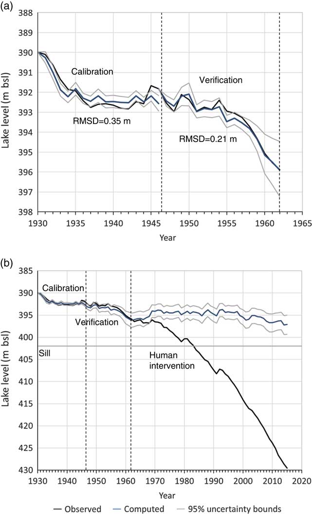
A potentially weak point in the model’s development is the use of data only from high lake levels (>396 m bsl), as no data are available from low levels under natural conditions. This means that the application of the model to drier intervals in which low lake levels are simulated should be approached with caution.
Lake level without anthropogenic intervention
Figure 5b presents the model application for 1930–2015 and demonstrates what would have been the current Dead Sea levels under natural conditions, without the intensive human impact and the diversion of water out of the watershed. According to the model, an over 6-m decline in lake level is predicted under natural conditions from the 1930s to mid-1960s. Then, a rise of more than 2 m in 5 yr is predicted due to a series of wet years (including the exceptional, wettest year on record in the northern part of the watershed, 1968/1969, with >1300 mm annual precipitation; Fig. 6a) that would have been followed by relatively stable levels for the subsequent 30 yr. According to the model, a slow decline in lake level (~3 m in 20 yr) should have occurred from the mid-1990s to 2015 but, surprisingly, the lake level would have remained above the sill at 397 m bsl in 2015. Thus, under natural conditions, the southern basin would have been flooded and the Dead Sea would have been a larger lake than it is today. In reality, lake levels have declined ~30 m during the 45 yr since the early 1970s, and the southern basin is disconnected. This is due mostly to the large water diversion from the northern watershed of the Dead Sea and, to a lesser degree, to the industrial activities within the lake basin. The 95% uncertainty range for the analyzed interval varies between 0.3 and 2.4 m, and it is 1.4 m on average.
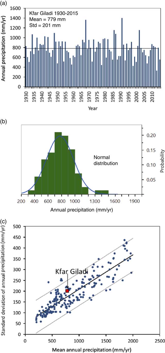
(a) Annual precipitation data at Kfar Giladi station (blue bars), mean value (black line), and statistics, and (b) normal distribution fit (blue line) to annual precipitation (green bar histogram); P-value=0.31 for Shapiro-Wilk W test indicates that the normal distribution null hypothesis cannot be rejected. (c) Scatter plot (blue circles) of annual precipitation standard deviation versus mean annual precipitation for stations in Europe and the Middle East obtained from the European Climate Assessment and Dataset database (Tank et al., Reference Tank, Wijngaard, Können, Böhm, Demarée, Gocheva and Mileta2002). Black line represents the linear fit and the rectangle represents Kfar Giladi station data for 1930–2015. The derived linear relationship (Eq. 4) has R 2 of 0.79. (For interpretation of the references to color in this figure legend, the reader is referred to the web version of this article.)
The model and its parameters obtained using present-day data are applied to the late Holocene in the following sections. This assumes that no changes in watershed settings during that period caused any substantial changes in precipitation-lake-inflow relationships and, in particular, watershed vegetation and potential evapotranspiration are similar to conditions during the model-development interval. This assumption is supported by different studies on speleothem records and confirms that during the late Holocene, vegetation (Keinan, Reference Keinan2016), air temperature, relative humidity (Affek et al., Reference Affek, Bar-Matthews, Ayalon, Matthews and Eiler2008), and sea surface temperature (Almogi-Labin et al., Reference Almogi-Labin, Bar-Matthews, Shriki, Kolosovsky, Paterne, Schilman, Ayalon, Aizenshtat and Matthews2009) over the eastern Mediterranean were mostly similar to present-day conditions.
RECONSTRUCTING LATE HOLOCENE PRECIPITATION SCENARIOS USING A STOCHASTIC FRAMEWORK
Processes in the atmospheric and hydrological systems have some stochastic components, with an element of randomness manifested in each of the system's parameters (Wilks, Reference Wilks2011). Considering this, it is assumed that these systems can randomly generate different records, termed realizations, which share given statistical properties such as mean and variance. Generating an ensemble of synthetic annual precipitation realizations and applying them as input into the water-balance model (i.e., Monte Carlo simulation) enables examining a large variety of lake-level changes that might be obtained for a given precipitation regime (i.e., precipitation statistics). The advantage of using an ensemble of realizations, rather than a single record, as inputs to the model is that it allows examining the discussed system under large variance, which ideally represents the natural conditions, and to assess probabilities of lake-level changes under different scenarios.
The above ideas are utilized in the stochastic framework as follows: (1) precipitation ensembles are generated representing different scenarios of precipitation regime; (2) the precipitation ensembles serve as input to the water-balance model to compute lake-level ensembles for the different scenarios; (3) lake-level gradients are derived for each realization and for each examined scenario; (4) probabilities of lake-level gradients under examined scenarios are determined. Using this stochastic framework, we consider the reconstructed lake-level curve (Bookman et al., Reference Bookman, Enzel, Agnon and Stein2004; Fig. 2), specifically its rising and declining intervals, and assess which precipitation scenarios are more likely to cause such changes. The initial lake level and the duration of each examined interval can affect the derived gradients and are therefore included in the analysis.
Statistical properties of annual precipitation data and precipitation ensembles
Precipitation regime is represented here by the statistical properties of annual precipitation data (i.e., mean, standard deviation, probability distribution, and autocorrelation). For present-day climatic conditions, the statistical properties of the randomly generated synthetic annual precipitation data should match those of observations, whereas those properties need to be altered for wetter or drier conditions.
The Kfar Giladi annual precipitation data for 1930–2015 were examined (Fig. 6a). The MAP is 779 mm/yr, with a standard deviation of 201 mm/yr and an insignificant lag-1 autocorrelation (R<0.001), supporting the assumption of independence between precipitation amounts in two consecutive years. While we concluded that normal, lognormal, and gamma distribution functions fit the annual precipitation record, the normal distribution was selected for further analysis (Fig. 6b) due to its convenient properties and the possibility of changing the parameters, namely, the mean, µ, and standard deviation, σ, of the annual precipitation, to represent different climatic regimes, as explained below.
To simulate drier and wetter climatic conditions, we examined the relations between the two normal distribution parameters for a range of precipitation regimes. We used precipitation records of the European Climate Assessment and Dataset (ECA&D; Tank et al., Reference Tank, Wijngaard, Können, Böhm, Demarée, Gocheva and Mileta2002) containing long-term high-quality daily observational series from stations in Europe and the Mediterranean. Annual precipitation data were computed, and station records were included in the analysis if three conditions were met: (1) at least 40 yr of data are available for the 50-yr span of 1960–2010, (2) MAP is in the range of 200–2000 mm/yr, and (3) precipitation in October–May comprises at least 70% of the annual precipitation. The normal distribution showed a good fit with most (more than 95%) of the 215 stations that met the above criteria in the database used. The relationships between MAP and standard deviation of annual precipitation were close to linear (Fig. 6c). This linear relationship was used to derive the standard deviation parameter σ for any simulated MAP µ:
 $$\sigma {\equals}0.16{\times}\mu {\plus}50$$
An underlying assumption is that the above relationship, obtained from present-day climatic conditions in the Mediterranean and Europe, is also valid for the late Holocene. Other probability-distribution functions (lognormal and gamma) also fit the data well in many cases, but an adequate method for shifting between precipitation regimes could not be identified, supporting use of the normal distribution for the current study.
Based on the above analysis of data from 215 stations, we used a random number generator to produce ensembles, each composed of 1000 annual precipitation time series (precipitation realizations) with the following assumptions: (1) normal distribution well represents the regional annual precipitation (Fig. 6a and b); (2) a linear relationship exists between normal distribution parameters and the mean and variance of annual precipitation (Fig. 6c, Eq. 4); and (3) the annual precipitation values are independent (supported by a negligible lag-1 autocorrelation). The precipitation ensembles representing different scenarios, as explained below, are the input to the water-balance model and resulted in ensembles of 1000 computed lake-level time series (lake-level realizations).
MAP versus mean lake-level relations utilizing static precipitation regime scenarios
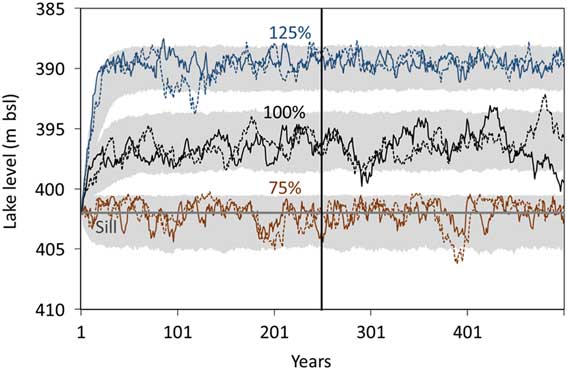
As a first step, we considered scenarios of static precipitation regimes, i.e., constant MAP, where lake levels are expected to vary around a stable mean. We examined precipitation regimes with annual means between 60 and 140% of the current Kfar Giladi MAP. Ensembles of 1000 realizations, each 500-yr long, were produced for each examined mean, where the MAP was kept constant for the entire simulation and standard deviation was set according to Equation 4. The precipitation ensembles served as input to the water-balance model where the initial lake-level conditions were set to the sill level (402 m bsl).
Figure 7 presents examples of two arbitrarily selected computed lake-level time series and the 95% lake-level range, for scenarios with 75, 100, and 125% of the present-day Kfar Giladi MAP. The first part of the computed lake level series depends on the initial conditions; however, this dependency vanishes after 100–200 yr and, therefore, we consider only the last 250 yr of the computed lake level series for further analysis. Figure 7 also indicates that lake level varies in time around a mean lake level and that these lake-level variations represent natural, interannual changes in annual precipitation.
Example of stochastic lake-level simulations for scenarios with 75% (brown), 100% (black), and 125% (blue) of the Kfar Giladi present-day mean annual precipitation. For each scenario, two arbitrarily selected, computed lake-level time series are presented (solid and dashed lines). The 95% lake-level range from all simulations in each scenario is presented in gray. Initial lake-level conditions were set in all cases to the sill level (402 m bsl). (For interpretation of the references to color in this figure legend, the reader is referred to the web version of this article.)
The derived relationship between Kfar Giladi MAP and mean lake level is shown in Figure 8. It indicates that the current Kfar Giladi MAP is associated with a mean lake level of 396 m bsl, which is a rare high lake level during the late Holocene (Fig. 2). This outcome indicates that the modern MAP represents a relatively wetter interval in the Holocene, a dire implication for future regional water resources. The more common lake levels during the late Holocene are associated with the sill level (402 m bsl; Fig. 2). At Kfar Giladi, this level corresponds to 586 mm/yr MAP (Fig. 8) or only 75% of the present-day conditions. Consequently, this value of 586 mm/yr in Kfar Giladi is referred to hereafter as the “reference MAP”. In other words, it replaces the present-day mean—the commonly used reference MAP—which is much too high.
Relationship between Kfar Giladi mean annual precipitation (MAP) and mean lake level (blue line) obtained from ensembles of annual precipitation with a constant mean and variance and ensembles of computed lake level. Gray lines represent the 95% range of lake levels for each MAP value. Vertical red line indicates the current conditions, without anthropogenic intervention, of the natural system. Vertical green line shows the conditions associated with lake level at the elevation of the sill (402 m bsl), suggested here as the reference MAP. For each case, MAP, mean lake level, and 0.025 and 0.975 quantiles (q0.025 and q0.975, respectively) are given. (For interpretation of the references to color in this figure legend, the reader is referred to the web version of this article.)
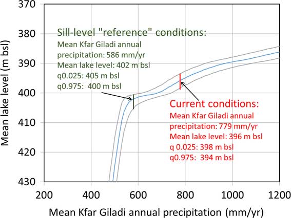
It is interesting to note the different slopes of the curve presented in Figure 8, with a large change in the slope of the response around the sill level. This means that below this point, a further decrease in MAP leads to a large decrease in the expected mean lake level. In contrast, an increase in mean precipitation above this level leads, on average, to a small increase in lake level. In other words, the increase in MAP needed to raise the water level is significantly larger once it is above the sill elevation compared to when the water level is below the sill elevation. This behavior can be attributed to two effects occurring with increasing lake level above the sill: (1) water is less saline and its density is lower (Fig. 3a), and evaporation rate increases (Fig. 3b), (2) lake surface area increases as the southern basin is flooded. Both factors contribute to large evaporation volumes, requiring higher precipitation amounts to be balanced. On the other hand, as lake level decreases below the sill level, the change in density (more saline), and hence evaporation rate, is smaller (Fig. 3a and b), and lake surface area is reduced. It should be emphasized that this behavior refers to mean precipitation and mean lake levels under static conditions, but a given realization can lead to a temporary increase and decrease of lake levels, as can be seen in Figure 7. Furthermore, lake level realizations tend to vary more at low lake levels (lower than the sill) compared to higher lake levels, as manifested in the vertical distance between the gray lines plotted in Figure 8 representing 95% of lake levels for each MAP value. This indicates the increased sensitivity of lake level to precipitation, as described above.
MAP trend scenarios and probabilities of lake level rises and declines
As stated earlier, using the stochastic framework, it is possible to estimate probabilities of lake level gradients under a given precipitation scenario. In this section, we consider the rises and declines in the reconstructed Dead Sea level (Fig. 2) and look into which precipitation scenarios could have led to such changes. Although under the static MAP scenarios presented above, a random series of dry or wet years around a mean can lead to rises and declines of lake levels (e.g., Fig. 7), the more general case is a MAP trend with the zero trend being the static case. Here we examine linear trend scenarios in which the Kfar Giladi MAP changed during the years of the simulations, using negative and positive linear trends of up to 50 mm/10 yr. As before, the standard deviation for each simulated year was set according to Equation 4.
The reconstructed late Holocene lake level (Fig. 2) was divided into 12 intervals with systematic rises and declines (Table 4). The older part of the reconstructed lake level, 2500–500 BC, includes uncertain rapid changes (dashed lines, Fig. 2) that were not considered here. Rather, mean lake level gradients for ~1000-yr intervals were considered for this period. After 500 BC, the curve is more certain and we analyzed shorter intervals (<420 yr). The most recent analyzed interval was AD 1900–1963, thereby avoiding human-impacted lake levels.
Analyzed intervals and their properties.

For each examined interval, we produced ensembles of precipitation scenarios, each consisting of 1000 realizations, based on the Kfar Giladi MAP that incorporated increasing or decreasing trends over the same duration as the considered interval. The observed lake level at the beginning of each interval was taken as the initial lake level for the simulation and the MAP in the first year of the simulation was derived from the initial lake level by applying the relationships presented in Figure 8 (Table 4).
Each examined precipitation scenario resulted in an ensemble of 1000 computed lake level realizations, and their statistical properties were analyzed. Specifically, the mean lake level gradient (in m/100 yr) of each realization was computed as the difference between the final and initial lake levels divided by the interval duration. For each ensemble, representing a given precipitation trend scenario, the probability distribution of lake level gradients was determined from all 1000 realizations in the ensemble. These are the lake level gradients expected under the given precipitation scenario when the natural variability of annual precipitation is taken into account.
Consider, for example, the 360-yr interval (80 BC–AD 280) in which lake level, according to the reconstructed curve (Fig. 2), declines from 394.5 to 404.5 m bsl. We examine different trends of MAP in the range of -50 to +50 mm/10 yr, where lake level is 394.5 m bsl and MAP is 814 mm for the first year (from Fig. 8).
For each examined interval (Table 4), one can utilize the derived probability distributions and determine how likely a given observed lake level gradient is under a given precipitation scenario. The P value of the observed gradient is estimated as the percentage of lake level realizations with equal or steeper gradient than that observed. If the P value is larger than a preselected significance level (in our case 5%), then the MAP trend scenario is defined as allowable for the specific interval analyzed, since the observed lake trend could have been generated by chance when this MAP trend is dominant. Furthermore, we define the most probable MAP trend scenario associated with a given lake level trend as the one with the largest P value.
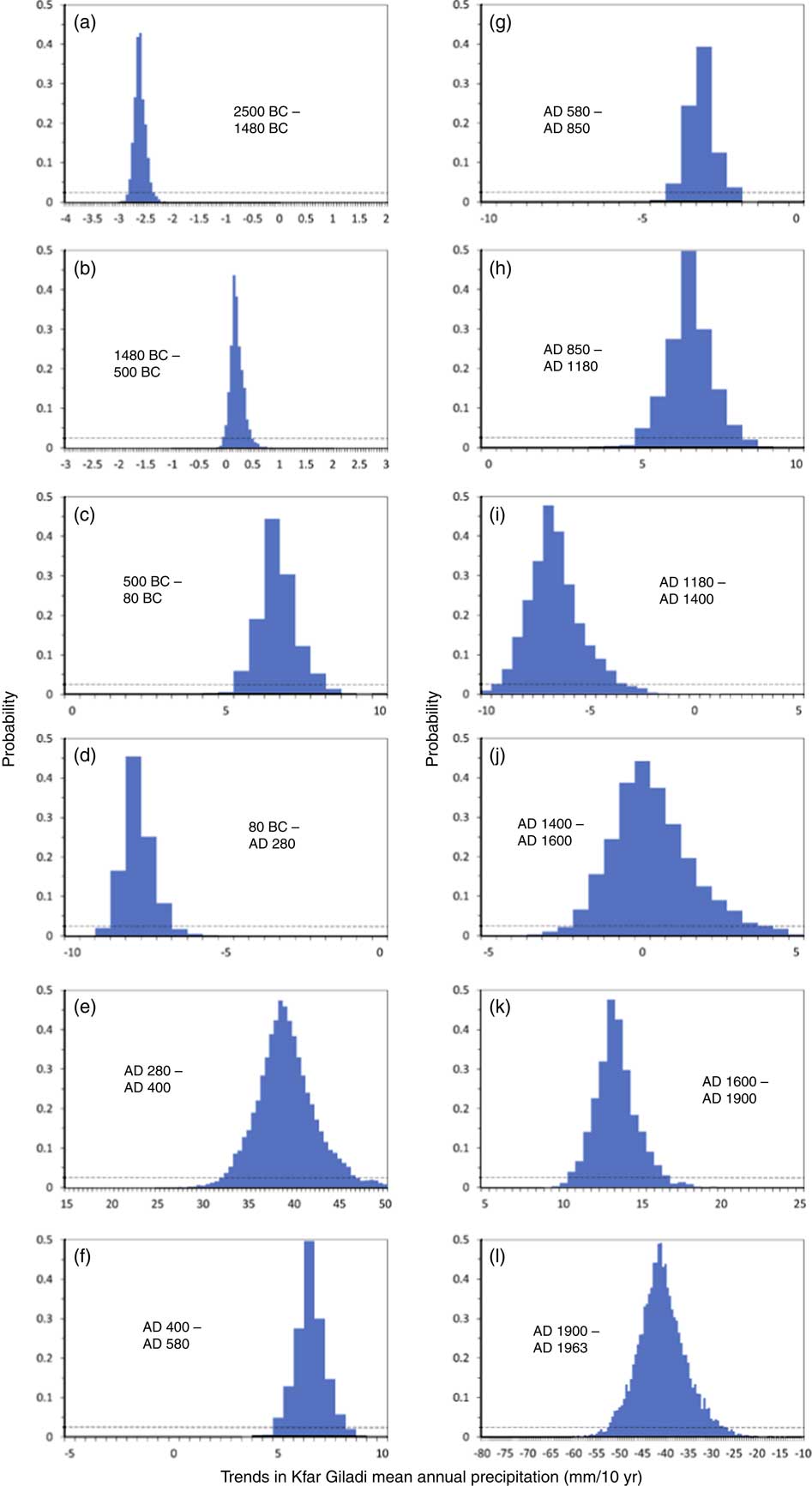
The derived P values for a range of analyzed MAP trend scenarios for each analyzed interval of the reconstructed lake level are shown in Figure 9. The allowable and most probable MAP trends for each interval are presented in Table 4. Except for one case (AD 1400–1600), zero trend (i.e., constant MAP) is not allowable in any interval. This means that under constant MAP conditions, the rises and declines observed in the reconstructed lake level curve have a very low chance of occurring. On the other hand, under MAP trend scenarios, these lake level gradients are more probable.
(color online) Probabilities of obtaining lake-level changes or more extreme changes (i.e., P-value) for 12 intervals of reconstructed Dead Sea level (Figure 10a, Table 4) for different trends in mean annual precipitation at Kfar Giladi. The trend with the maximal probability is considered to be the most probable precipitation trend and the range of trends above the 5% significance level (dashed line) are the allowable precipitation trends for the considered lake-level gradient (Table 4).
Reconstruction of late Holocene precipitation regime
The most probable MAP trend scenarios associated with different intervals of rises and declines in the reconstructed Dead Sea level (Fig. 2) were used to reconstruct Levant precipitation mean, variance, and trends during the late Holocene. The lake level model was run continuously for the entire studied period, starting at 4500 yr before the present with a lake level of 396 m bsl and a MAP of 779 mm/yr (first row in Table 4), applying the most probable MAP trend for each interval; 1000 such runs were made, accounting for the annual precipitation variance (a function of MAP; Eq. 4), thereby producing an ensemble of 1000 realizations, each 4500-yr long, of Kfar Giladi annual precipitation and the associated lake level. The reconstructed MAP in Kfar Giladi during the late Holocene deduced from these realizations is shown in Figure 10b as a black line, along with an arbitrarily selected annual precipitation realization, and the 95% range of annual precipitation (i.e., for each year the range between the 2.5 and 97.5% quantiles from all realizations). Obviously, founding this analysis on the typically low-resolution reconstructed lake-level data, it is impossible to identify short-term MAP trends. Even though it is reasonable to assume that precipitation trends are not constant within intervals longer than ~100 yr, no information exists to identify such changes. Therefore, the trend analysis provides information on the mean behavior during the defined intervals.
Reconstructed precipitation and lake level for the late Holocene. (a) Reconstructed Dead Sea level (after Bookman et al., Reference Bookman, Enzel, Agnon and Stein2004); sill level is shown as a thick gray line. The dashed vertical lines divide the 4500 yr into 12 intervals of relatively constant lake-level gradients. Uncertain rapid changes during 1480–500 BC (shown as dashed lines) are not considered. (b) Ensemble of reconstructed late Holocene annual precipitation at Kfar Giladi derived from the most probable precipitation trend for each of the 12 intervals in the Dead Sea level curve; the ensemble median is shown as a black line, arbitrarily selected annual precipitation realization as a blue line, and the 95% lake-level range from all 1000 ensemble realizations is in gray. The mean annual precipitation associated with the sill level is shown as a gray line, and mean annual precipitation for the present-day record is shown as a red dot on the left. A second y-axis shows precipitation values relative to modern mean annual precipitation. (c) Ensemble of computed late Holocene lake level; ensemble median (black line), computed lake level for the selected realization (green line), 95% computed lake-level range (gray area), and sill level (gray line). (For interpretation of the references to color in this figure legend, the reader is referred to the web version of this article.)
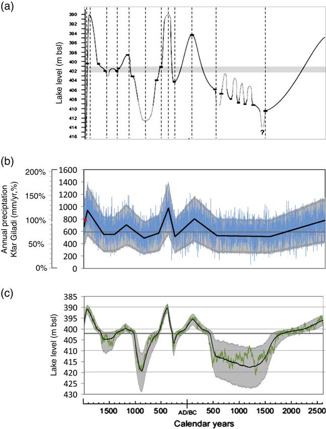
The ensemble mean computed lake level, the 95% range, and the lake level computed from the selected realization are shown in Figure 10c. As expected, the lake-level ensemble median (Fig. 10c, black line) is similar to the lake level reconstructed by Bookman et al. (Reference Bookman, Enzel, Agnon and Stein2004; Fig. 10a). The arbitrarily selected single lake-level realization (green line in Fig. 10c) is smoother than the corresponding precipitation realization (blue line in Fig. 10b) but, as expected, it is still noisier than the lake-level ensemble median (black line in Fig. 10c). These realizations present smaller-scale rises and declines, reflecting random clusters of high or low precipitation amounts. It is clear from Figure 10c, as already mentioned earlier, that at low lake levels, the spread of the realizations is much larger than at high lake levels, resulting in the thicker gray area below the sill.
The MAP at the station (Kfar Giladi) varied in the range of 489–975 mm, i.e., 83–166% (63–125%) of the reference (present-day) MAP. The two driest intervals of the late Holocene are 1500–1200 BC and AD 755–890 (Fig. 10b). In these intervals, MAP declined to 83–88% (63–66%) of the reference (present-day) Kfar Giladi MAP. Under present-day climate, stations with a similar MAP are located at approximately 1° latitude (~100 km) south of Kfar Giladi (Fig. 1). We note that, due to the high interannual variance, precipitation in a single year could be much lower or higher than the MAP range. For example, consider the relatively dry interval of AD 850–1180 (Table 4): the annual precipitation in the realization presented in Figure 10b during this period reached a maximum of 1027 mm, which is considered a very wet year even under the present-day climate; i.e., extremes that are opposite to the general trend can occur, albeit rarely.
The late Holocene's wettest intervals are 2500–2460 BC, 130–40 BC, AD 350–490, and AD 1770–1940 (Fig. 10b). During these intervals, the Kfar Giladi MAP varied from 131–166% (99–125%) of its reference (present-day) MAP. In the present-day climate, stations with a similar MAP are located approximately 1° north of Kfar Giladi (Fig. 1). These 1° shifts in MAP indicate changes in the regional synoptic-scale conditions.
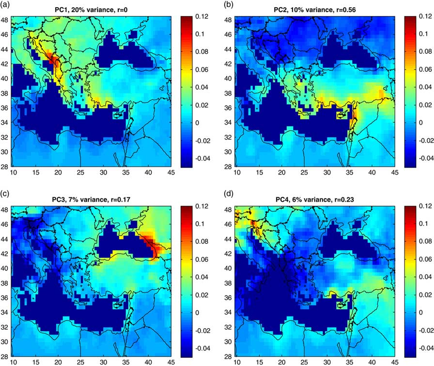
The modern Levant annual precipitation is spatially coherent (Fig. 4; Enzel et al., Reference Enzel, Bookman (Ken Tor), Sharon, Gvirtzman, Dayan, Ziv and Stein2003). Therefore, we postulate that the identified MAP trends over the past 4500 yr (Fig. 10b) are applicable to the entire Levant. These changes in MAP are most likely related to changes in tracking and frequency of eastern Mediterranean cyclones (Enzel et al., Reference Enzel, Bookman (Ken Tor), Sharon, Gvirtzman, Dayan, Ziv and Stein2003; Saaroni et al., Reference Saaroni, Halfon, Ziv, Alpert and Kutiel2010). Principal component analysis of annual precipitation (1923–2012) in the eastern Mediterranean (Fig. 11) applied to data from the GPCC data set (Schneider et al., Reference Schneider, Becker, Finger, Meyer-Christoffer, Ziese and Rudolf2014) shows that the second component (explaining 10% of the variance) is related to precipitation in the Levant region; it is the only component with a correlation of >0.5 with annual precipitation in Kfar Giladi (Fig. 11b). Therefore, it is suggested that this mode is controlled by the southeastern storm track over the Mediterranean. It is further postulated that, during intervals characterized by high regional MAP, this component is strong in most years, whereas the southeastern storm track component is weak during low MAP intervals. Further research is required to examine this assumption.
(color online) The first four principal components of annual precipitation (September–August) for 1923–2012 from Global Precipitation Climatology Centre 0.5° monthly precipitation data (Schneider et al., Reference Schneider, Becker, Finger, Meyer-Christoffer, Ziese and Rudolf2014). Colors represent principal component loadings. The principal components explained the variance, and the correlation (R) of its scores with annual precipitation at Kfar Giladi station are shown. The second principal component (b) is related to precipitation in the Levant region; it is the only component with R>0.5 with the Kfar Giladi annual precipitation.

DISCUSSION
Variations in the Levant climate during the late Holocene were documented by the Dead Sea levels that represent alterations between decadal- and centennial-scale wetter and drier intervals. The question of the magnitudes of these alterations has only been partially discussed in previous studies (e.g., Enzel et al., Reference Enzel, Bookman (Ken Tor), Sharon, Gvirtzman, Dayan, Ziv and Stein2003; Litt et al., Reference Litt, Ohlwein, Neumann, Hense and Stein2012). In the current study, we aimed to provide quantitative estimates of precipitation associated with late Holocene lake levels and rises and declines in lake levels, focusing on the means and trends of annual precipitation while accounting for interannual variability. Here we discuss the main conclusions and their implications.
The MAP during the late Holocene is estimated to range between 63 and 125% of the present-day mean value for the Kfar Giladi station. When the lake was at sill level (402 m bsl), MAP at Kfar Giladi was only 75% of its current value. Although this assessment is based on a single station, it is supported by the high correlation between the Kfar Giladi annual precipitation and annual lake-level changes (Table 1), the high spatial correlation of annual precipitation in the region (Fig. 4), and previous studies indicating high spatial coherence of annual precipitation in the southern Levant (Enzel et al., Reference Enzel, Bookman (Ken Tor), Sharon, Gvirtzman, Dayan, Ziv and Stein2003). Lake level hovering near the sill level was much more common during the late Holocene than the high lake stands at the beginning of the twentieth century (Fig. 2). Therefore, we propose that the MAP associated with the sill level should be regarded as the “reference MAP” rather than the commonly used present-day precipitation mean. According to our reconstructed data, the Kfar Giladi MAP in AD 1900 was 940 mm/yr (close to the late Holocene MAP maximum of 975 mm/yr; Fig. 10b). Since then, there has been a drying trend and the MAP trends down toward lower, more common values. One can thus view the present drying trend as a falling limb of the natural variations and a return to the common late Holocene state of precipitation and, as a result, to the common reference lake level. The reported regional drying in recent decades (Shohami et al., 2011; Kelley et al., Reference Kelley, Mohtadi, Cane, Seager and Kushnir2015) probably represents a superposition of this natural trend and human-induced climatic changes, but separating them is beyond the scope of this study.
The analysis presented in this paper utilizes a stochastic framework to account for interannual variability of annual precipitation on the decadal to centennial scale. The main advantages of this approach are: (1) it allows differentiating between (a) lake-level changes caused by natural variability of annual precipitation, and (b) occasional episodes characterized by clustering of wet or dry years that are associated with true and probably important changes in precipitation regime; (2) it provides probability assessments of lake-level trends under different precipitation scenarios. Considering the typical high variability of precipitation, this approach allows for a more realistic assessment of changes in precipitation regime as compared to the more standard and commonly used deterministic approach. This methodology can be applied to other world regions with similar settings, and thus can lead to a more accurate quantitative assessment of past precipitation regimes and magnitudes of climate changes.
Several simplified assumptions underlying the above analysis should be reiterated: (1) invariance in the relationship between precipitation and lake inflow volume (Eq. 3) throughout the late Holocene, and (2) negligible effects of intra-annual and intra-watershed variations in precipitation. The first assumption is justified since no substantial changes in watershed structure or in the general climatic circulation affecting the region are known for the considered time period. The second assumption is supported by the generally high R 2 obtained between annual precipitation amounts measured at several stations and lake-level changes (Table 1), indicating that the lake’s annual water budget is mainly controlled by the total annual precipitation, which has been attributed to the strong underground flow paths of a large fraction of the water discharged into the lake (e.g., most of the Upper Jordan River stream flow is from underground; Rimmer and Salinger, Reference Rimmer and Salingar2006). Although a significant fraction of the watershed area, mainly to the south of the lake, is characterized by arid to hyperarid climate and increased sensitivity of runoff to spatial and temporal variations in precipitation (e.g., Morin and Yakir, Reference Morin and Yakir2014), the water inflow to the lake from this part of the watershed is minimal compared to the wetter northern region (Greenbaum et al., Reference Greenbaum, Ben-Zvi, Haviv and Enzel2006). Furthermore, it has been shown that the southern area has remained arid to hyperarid since the middle Pleistocene and undoubtedly during the Holocene (e.g., Amit et al., Reference Amit, Enzel and Sharon2006; Enzel et al., Reference Enzel, Amit, Dayan, Crouvi, Kahana, Ziv and Sharon2008, Reference Enzel, Amit, Grodek, Ayalon, Lekach, Porat, Bierman, Blum and Erel2012). Lastly, the analysis in this paper is focused on the late Holocene, and may be extended to the entire Holocene. Extrapolation to the late Pleistocene cannot be justified, however, as climatic, environmental, and physiographic conditions were substantially different and thus the model settings must be altered.
The rate of change in MAP in the late Holocene (Table 4) is relatively small compared to the typically high interannual variance (Morin, Reference Morin2011). As a result, intervals of a few decades will not generate a definite perception of a change in precipitation regime to wetter or drier conditions. To demonstrate this, we computed, for each of the 12 intervals, the probability of detecting a statistically significant precipitation trend within a 50-yr interval. Only two of these cases generated probabilities exceeding 50%; as expected, this characterized only the steepest trends of 38.5 and −41 mm/10 yr (Table 4).
In contrast with the precipitation trends, trends in lake levels are much easier to identify due to their respective lower variances. The probability of detecting significant trends within any 50-yr interval in all 12 intervals is >60%. The lesson learned from this analysis is that short, undetectable precipitation trends (i.e., trends that were not found to be statistically significant due to the low signal-to-noise ratio, Morin, Reference Morin2011) can still cause substantial lake changes. Hydrological systems often amplify their climatic input signal under both wetting and drying conditions (e.g., Peleg et al., Reference Peleg, Morin, Gvirtzman and Enzel2011, who considered spring discharge response to precipitation changes). Thus, statistically insignificant precipitation changes may result in a significant change in the system's response. Consequently, we suggest that the interpretation of insignificant precipitation trends as “no change” should be made more cautiously (see Morin, Reference Morin2011 for further discussion).
CONCLUSIONS
Mean, variance and their trends of Kfar Giladi annual precipitation were calculated from the Dead Sea level curve over the past 4500 yr. Annual precipitation at the Kfar Giladi station is well-correlated with annual precipitation in the entire Levant and with Dead Sea level changes.
The reference late Holocene MAP at Kfar Giladi was 588 mm/yr, only 75% of the present-day value, and it is associated with Dead Sea sill elevation. Calculated MAP at Kfar Giladi varied over the late Holocene in the range of 489–975 mm/yr, −17 to +66% of the reference value (and a change of −37 to +25% from the present state). Under trends of MAP, Dead Sea rises and declines (from the reconstructed curve) have a much higher occurrence probability than under simple changes in stable mean precipitation. Most of the late Holocene precipitation regime can be characterized by >200-yr-long episodes of MAP trends of −15 to +15 mm/10 yr. Such trends are difficult to detect over decades. Trends in MAP most probably reflect shifts in eastern Mediterranean cyclone tracks; a relatively southern track brings larger amounts of precipitation to the Levant.
Present-day conditions (from the early twentieth century) are relatively wet if viewed in the context of the late Holocene perspective. If we adopt this view, the recent drying of the region can be partially explained as a return to the “normal” drier conditions. Nevertheless, without human intervention in the Dead Sea watershed, lake level as of 2015 would have remained above the sill and the southern basin would still be flooded.
The stochastic framework allows accounting for interannual variability and assessing probabilities of lake-level changes under different precipitation scenarios. The presented methodology can be applied to other global regions with similar settings, and thus can lead to a more accurate assessment of past precipitation regimes.
ACKNOWLEDGMENTS
The study was partially funded by the Israel Science Foundation (ISF grant no. 1007/15). It is a contribution to the PALEX project “Paleohydrology and Extreme Floods from the Dead Sea ICDP Core” funded by the Deutsche Forschungsgemeinschaft (DFG grant no. BR2208/13-1/-2), by ISF–Dead Sea Core Center of Excellence (ISF grant no. 1436/14) by the Israel Ministry of Science and Technology (grant no. 61792) and by U.S. National Science Foundation (NSF) – U.S.-Israel Binational Science Foundation (BSF) grant (BSF 2016953). Constructive reviews by Emi Ito, Steven Bacon, Associate Editor Xiaoping Yang, and Senior Editor Derek Booth improved the manuscript. This work is a contribution to the HyMeX program. We acknowledge the data providers in the ECA&D project. Klein Tank, A.M.G. and Coauthors, 2002. Daily dataset of 20th-century surface air temperature and precipitation series for the European Climate Assessment. Int. J. of Climatol., 22, 1441-1453. Data and metadata available at http://www.ecad.eu


 Open access