





1. Introduction
Most droplet impact research concerns normal collisions with a static substrate. However, in many natural and industrial processes, droplets impact obliquely or onto a moving substrate. This seemingly subtle distinction transforms droplet impact from the typical axisymmetric configuration to be inherently three-dimensional. Example processes include raindrops splashing on the moving ocean that contributes to air–sea exchange (Anguelova Reference Anguelova2021), inkjet printing onto moving paper (Lohse Reference Lohse2022), and crop spraying with numerous droplet impacts at arbitrary angles (Gielen et al. Reference Gielen, Sleutel, Benschop, Riepen, Voronina, Visser, Lohse, Snoeijer, Versluis and Gelderblom2017).
Most of the existing literature on moving substrates has considered dry surfaces, where horizontal surface motion can modify splashing thresholds (Bird, Tsai & Stone Reference Bird, Tsai and Stone2009; Hao & Green Reference Hao and Green2017), alter spreading factors (Li et al. Reference Li, Shang, Wang and Zhang2024), and even generate new impact outcomes such as boundary-layer-driven ‘aerodynamic rebound’ (Stumpf et al. Reference Stumpf, Qezeljeh, Kamal, Dezitter, Martuffo, Roisman and Hussong2025). Likewise, inclined solid surfaces yield asymmetric crowns and reduce splashing propensity (Hao et al. Reference Hao, Lu, Lee, Wu, Hu and Floryan2019).
When the substrate is a pool, either moving or with a droplet impacting obliquely, the literature is more limited and exploratory. Castrejón-Pita et al. (Reference Castrejón-Pita, Muñoz-Sánchez, Hutchings and Castrejón-Pita2016) identified distinct regimes (including a new ‘surfing’ outcome) that depend on the pool–droplet speed ratio, but could not explore low pool speeds. Several studies have considered thin films that are either flowing (Guo et al. Reference Guo, Xu, Wang, Tian, Zhao and Zhu2025) or obliquely impacted (Bao et al. Reference Bao, Yi, Zhao, Liu, Guo, Gong and Shen2025). A few authors have considered oblique impact (Gielen et al. Reference Gielen, Sleutel, Benschop, Riepen, Voronina, Visser, Lohse, Snoeijer, Versluis and Gelderblom2017; Reijers et al. Reference Reijers, Liu, Lohse and Gelderblom2019), and moving (Gupta & Kumar Reference Gupta and Kumar2020), deep pools. However, all of these works focused on long time scale dynamics such as crater evolution, crown structure and the Worthington jet.
For static pools, following the observation that high-speed droplet impact leads to the formation of an ejecta sheet (Weiss & Yarin Reference Weiss and Yarin1999; Thoroddsen Reference Thoroddsen2002), it is now well understood that the ejecta sheet dynamics on very short time scales determine impact outcomes (Wang et al. Reference Wang, Liu, Bayeul-Lainé, Murphy, Katz and Coutier-Delgosha2023). Using X-ray imaging, Zhang et al. (Reference Zhang, Toole, Fezzaa and Deegan2012) confirmed that at low Reynolds numbers $\textit{Re}$
, a single sheet-like jet (termed a lamella) is formed by droplet impact on a deep pool. The lamella subsumes the ejecta sheet, which collects fluid from the pool as it develops. At higher
$\textit{Re}$
, a single sheet-like jet (termed a lamella) is formed by droplet impact on a deep pool. The lamella subsumes the ejecta sheet, which collects fluid from the pool as it develops. At higher $\textit{Re}$
, the ejecta sheet remains a separate structure and is later accompanied by a roll jet, using the nomenclature of Agbaglah et al. (Reference Agbaglah, Thoraval, Thoroddsen, Zhang, Fezzaa and Deegan2015). A variety of dynamics associated with the ejecta sheet in the latter regime are seen, including the protrusion, quartering, and irregular splashing outcomes identified by Thoraval et al. (Reference Thoraval, Takehara, Etoh, Popinet, Ray, Josserand, Zaleski and Thoroddsen2012). At high
$\textit{Re}$
, the ejecta sheet remains a separate structure and is later accompanied by a roll jet, using the nomenclature of Agbaglah et al. (Reference Agbaglah, Thoraval, Thoroddsen, Zhang, Fezzaa and Deegan2015). A variety of dynamics associated with the ejecta sheet in the latter regime are seen, including the protrusion, quartering, and irregular splashing outcomes identified by Thoraval et al. (Reference Thoraval, Takehara, Etoh, Popinet, Ray, Josserand, Zaleski and Thoroddsen2012). At high $\textit{Re}$
in the irregular splashing regime, Thoraval et al. (Reference Thoraval, Takehara, Etoh, Popinet, Ray, Josserand, Zaleski and Thoroddsen2012) predicted from numerical simulations that the base of the ejecta sheet would be unstable and produce a von Kármán vortex street, which was experimentally observed by Castrejón-Pita et al. (Reference Castrejón-Pita, Castrejón-Pita and Hutchings2012). Here, we use the term separate ejecta sheet (SES) as an umbrella term for all non-lamella outcomes, which is consistent with Zhang et al. (Reference Zhang, Toole, Fezzaa and Deegan2012) and our previous work (Sykes et al. Reference Sykes, Cimpeanu, Fudge, Castrejón-Pita and Castrejón-Pita2023). Agbaglah et al. (Reference Agbaglah, Thoraval, Thoroddsen, Zhang, Fezzaa and Deegan2015) showed that the development of the SES outcome is driven by vortex shedding; the transition between a lamella and SES is associated with a fixed capillary number
$\textit{Re}$
in the irregular splashing regime, Thoraval et al. (Reference Thoraval, Takehara, Etoh, Popinet, Ray, Josserand, Zaleski and Thoroddsen2012) predicted from numerical simulations that the base of the ejecta sheet would be unstable and produce a von Kármán vortex street, which was experimentally observed by Castrejón-Pita et al. (Reference Castrejón-Pita, Castrejón-Pita and Hutchings2012). Here, we use the term separate ejecta sheet (SES) as an umbrella term for all non-lamella outcomes, which is consistent with Zhang et al. (Reference Zhang, Toole, Fezzaa and Deegan2012) and our previous work (Sykes et al. Reference Sykes, Cimpeanu, Fudge, Castrejón-Pita and Castrejón-Pita2023). Agbaglah et al. (Reference Agbaglah, Thoraval, Thoroddsen, Zhang, Fezzaa and Deegan2015) showed that the development of the SES outcome is driven by vortex shedding; the transition between a lamella and SES is associated with a fixed capillary number ${\textit {Ca}}=0.2$
. Here, we extend our knowledge of ejecta sheet behaviour to include pool movement, showing that impact outcomes can differ upstream and downstream only when
${\textit {Ca}}=0.2$
. Here, we extend our knowledge of ejecta sheet behaviour to include pool movement, showing that impact outcomes can differ upstream and downstream only when ${\textit {Ca}}\lt 0.2$
. The transition can be explained by considering the evolution of the ejecta sheet angle, giving a length-scale invariant parametrisation of
${\textit {Ca}}\lt 0.2$
. The transition can be explained by considering the evolution of the ejecta sheet angle, giving a length-scale invariant parametrisation of $\textit {Ca}$
and the square root of the pool–droplet velocity ratio.
$\textit {Ca}$
and the square root of the pool–droplet velocity ratio.
2. Methods
2.1. Experiments
Millimetric droplets were dripped from a blunt-end dispensing tip and impacted normally onto a deep pool, both consisting of the same fluid: distilled water, five glycerol–water mixtures, and two silicone oils – see table 1, where fluid properties and absolute errors (used in propagation of error analyses) are tabulated. Six dispensing tips (15–30 gauge, outer diameters 0.31–1.83 mm) were used to modify the droplet diameter $D\in [2.20,3.75]\,\textrm {mm}$
, which provides our characteristic length scale via the circle-fitted nominal radius
$D\in [2.20,3.75]\,\textrm {mm}$
, which provides our characteristic length scale via the circle-fitted nominal radius $r_n$
(see the supplementary material available at 10.1017/jfm.2026.11586.). The dispensing tip height relative to the pool free surface was varied (205–575 mm) to adjust the normal impact velocity,
$r_n$
(see the supplementary material available at 10.1017/jfm.2026.11586.). The dispensing tip height relative to the pool free surface was varied (205–575 mm) to adjust the normal impact velocity, $u_n\in [1.6,3.2]\ \textrm {m s}^{-1}$
. Absolute errors of
$u_n\in [1.6,3.2]\ \textrm {m s}^{-1}$
. Absolute errors of $\pm {0.01}\,\textrm{m}$
for
$\pm {0.01}\,\textrm{m}$
for $r_n$
and
$r_n$
and $\pm {0.01}\ \textrm{m s}^{-1}$
for
$\pm {0.01}\ \textrm{m s}^{-1}$
for $u_n$
are assumed. The variation in
$u_n$
are assumed. The variation in $u_n$
was primarily responsible for the range
$u_n$
was primarily responsible for the range ${\textit {We}}=\rho u_n^2D/\sigma \in [134,450]$
, while the different fluids enabled considerable variation in
${\textit {We}}=\rho u_n^2D/\sigma \in [134,450]$
, while the different fluids enabled considerable variation in $\textit{Re}=\rho u_n D/\mu \in [940,7930]$
(figure 1
a). As the capillary number
$\textit{Re}=\rho u_n D/\mu \in [940,7930]$
(figure 1
a). As the capillary number ${\textit {Ca}} = {\textit {We}}/\textit{Re} = \mu u_n/\sigma$
proves influential, we non-dimensionalise times with the visco-capillary time scale
${\textit {Ca}} = {\textit {We}}/\textit{Re} = \mu u_n/\sigma$
proves influential, we non-dimensionalise times with the visco-capillary time scale $\mu D/\sigma$
(dimensionless times are denoted by
$\mu D/\sigma$
(dimensionless times are denoted by $t_\mu ^\ast$
).
$t_\mu ^\ast$
).
Fluid properties of the droplet and pool (same fluid). The density of each glycerol–water mixture (glycerol, Acros Organics 99 % pure) was measured using a 25 ml density bottle and 1 mg precision analytical balance, dynamic viscosity with a vibrational viscometer (Hydramotion Viscolite 700, 0.1 mPa s precision), and surface tension with a Sinterface BPA-2S tensiometer. Measured viscosities were confirmed to be consistent with known empirical correlations (Cheng Reference Cheng2008). Silicone oils (Clearco Products) were used as received; the fluid properties reported are those from the product data sheet. All values are reported for $23\pm 1\,^\circ \textrm{C}$
.
$23\pm 1\,^\circ \textrm{C}$
.

For all experiments, the pool depth $h$
was maintained such that
$h$
was maintained such that $h/D\gt 3$
(typically with
$h/D\gt 3$
(typically with $h\in [12,14]\,\textrm {mm}$
), which is sufficient that the pool can be considered deep for the early-time dynamics of interest here (Thoroddsen et al. Reference Thoroddsen, Thoraval, Takehara and Etoh2011; Sykes et al. Reference Sykes, Cimpeanu, Fudge, Castrejón-Pita and Castrejón-Pita2023). Pool movement was achieved using a belt-driven rotating table fitted with an optically clear annular tank (figure 1
b) of outer diameter 588 mm (constructed from a 600 mm diameter cast acrylic tube with 6 mm wall thickness) and inner diameter 450 mm – see the supplementary material for further details. The inner walls were treated with a commercial hydrophobic coating (Rain-X Plastic Water Repellent) to curtail the formation of a meniscus that would interfere with side-view imaging. The experiments involving silicone oils used a similar set-up described in Harris et al. (Reference Harris, Alventosa, Sand, Silver, Mohammadi, Sykes, Castrejón-Pita and Cimpeanu2026). Using rotation to engender pool movement – as opposed to a simple linear translation of the pool – inevitably leads to a curved parabolic free surface in the direction orthogonal to the direction of pool movement, which is shown to be inconsequential for our results in § 3.6.
$h\in [12,14]\,\textrm {mm}$
), which is sufficient that the pool can be considered deep for the early-time dynamics of interest here (Thoroddsen et al. Reference Thoroddsen, Thoraval, Takehara and Etoh2011; Sykes et al. Reference Sykes, Cimpeanu, Fudge, Castrejón-Pita and Castrejón-Pita2023). Pool movement was achieved using a belt-driven rotating table fitted with an optically clear annular tank (figure 1
b) of outer diameter 588 mm (constructed from a 600 mm diameter cast acrylic tube with 6 mm wall thickness) and inner diameter 450 mm – see the supplementary material for further details. The inner walls were treated with a commercial hydrophobic coating (Rain-X Plastic Water Repellent) to curtail the formation of a meniscus that would interfere with side-view imaging. The experiments involving silicone oils used a similar set-up described in Harris et al. (Reference Harris, Alventosa, Sand, Silver, Mohammadi, Sykes, Castrejón-Pita and Cimpeanu2026). Using rotation to engender pool movement – as opposed to a simple linear translation of the pool – inevitably leads to a curved parabolic free surface in the direction orthogonal to the direction of pool movement, which is shown to be inconsequential for our results in § 3.6.
(a) Plots of $\textit {We}$
versus
$\textit {We}$
versus $\textit{Re}$
for all experiments reported. Error bars based on a propagation of error analysis (see § 2.1 for assumed absolute errors) would be smaller than each marker so are omitted. The purple line delineates the known vortex shedding boundary (
$\textit{Re}$
for all experiments reported. Error bars based on a propagation of error analysis (see § 2.1 for assumed absolute errors) would be smaller than each marker so are omitted. The purple line delineates the known vortex shedding boundary ( $\textit{Re}=5\,{\textit {We}}$
, i.e.
$\textit{Re}=5\,{\textit {We}}$
, i.e. ${\textit {Ca}}=0.2$
; Agbaglah et al. Reference Agbaglah, Thoraval, Thoroddsen, Zhang, Fezzaa and Deegan2015). (b) A rendering of the experimental set-up.
${\textit {Ca}}=0.2$
; Agbaglah et al. Reference Agbaglah, Thoraval, Thoroddsen, Zhang, Fezzaa and Deegan2015). (b) A rendering of the experimental set-up.

Figure 1. Long description
A scatter plot showing the relationship between Reynolds number and Weber number for different fluids, including glycerol-water mixtures, silicone oils, and water. The x-axis represents the Reynolds number ranging from 0 to 8000, and the y-axis represents the Weber number ranging from 150 to 450. The plot includes several data points color-coded by fluid type: purple for glycerol-water, orange for silicone oils, and light blue for water. A purple line indicates the vortex shedding boundary. The diagram on the right shows an experimental setup with a syringe pump, optical diffuser, front and back lights, and two cameras labeled Phantom Miro LAB310 and Phantom VEO 710L. The setup is used to study droplet impact on a moving substrate. All values are approximated.
Practical limitations restricted the maximum rotational frequency to approximately 0.5 Hz, with linear pool speeds at the impact point of ${u_t}\in [0,0.6]\ \textrm {m s}^{-1}$
reported here. The pool velocity
${u_t}\in [0,0.6]\ \textrm {m s}^{-1}$
reported here. The pool velocity $u_t$
was calculated from the rotation rate of the table, which was determined by monitoring the time for each quarter-rotation using an optical switch (Optek OPB900W55Z) connected to a data logger (Moku:Go). The implied
$u_t$
was calculated from the rotation rate of the table, which was determined by monitoring the time for each quarter-rotation using an optical switch (Optek OPB900W55Z) connected to a data logger (Moku:Go). The implied $u_t$
therefore assumes that the fluid is in solid-body rotation with the tank, and that the effect of air drag on the free surface is negligible. The typical time scale associated with spin-up of a fluid in a (non-annular) cylinder, from rest to angular velocity
$u_t$
therefore assumes that the fluid is in solid-body rotation with the tank, and that the effect of air drag on the free surface is negligible. The typical time scale associated with spin-up of a fluid in a (non-annular) cylinder, from rest to angular velocity $\varOmega$
, is
$\varOmega$
, is $t_E = {\textit {Ek}}^{-1/2}\varOmega ^{-1}=h\sqrt {\rho /\mu \varOmega }$
, where
$t_E = {\textit {Ek}}^{-1/2}\varOmega ^{-1}=h\sqrt {\rho /\mu \varOmega }$
, where ${\textit {Ek}} = \mu /\varOmega \rho h^2$
is the Ekman number (Greenspan & Howard Reference Greenspan and Howard1963). This time scale applies even when the cylinder is partially filled, since the bottom-wall Ekman layer is primarily responsible for spin-up (Homicz & Gerber Reference Homicz and Gerber1987), and is a factor of
${\textit {Ek}} = \mu /\varOmega \rho h^2$
is the Ekman number (Greenspan & Howard Reference Greenspan and Howard1963). This time scale applies even when the cylinder is partially filled, since the bottom-wall Ekman layer is primarily responsible for spin-up (Homicz & Gerber Reference Homicz and Gerber1987), and is a factor of ${\textit {Ek}}^{1/2}$
shorter than the viscous diffusion time scale due to the effect of Ekman suction. Here,
${\textit {Ek}}^{1/2}$
shorter than the viscous diffusion time scale due to the effect of Ekman suction. Here, $t_E \leq {40}\ \text{s}$
, which suggests that the allowed spin-up time of approximately 5 min for all experiments was sufficient. Particle tracking velocimetry experiments were also used to verify the actual free surface speeds – see the supplementary material (Crocker & Grier Reference Crocker and Grier1996). An absolute error
$t_E \leq {40}\ \text{s}$
, which suggests that the allowed spin-up time of approximately 5 min for all experiments was sufficient. Particle tracking velocimetry experiments were also used to verify the actual free surface speeds – see the supplementary material (Crocker & Grier Reference Crocker and Grier1996). An absolute error $\pm {0.02}\ \textrm{m s}^{-1}$
for
$\pm {0.02}\ \textrm{m s}^{-1}$
for $u_t$
is assumed, which typically dominates our propagated uncertainties (e.g. in figure 4 below).
$u_t$
is assumed, which typically dominates our propagated uncertainties (e.g. in figure 4 below).
Impacts were imaged from the side (through the side wall of the tank, figure 1
b) with a Phantom VEO 710L high-speed camera (7500–14 000 fps, 3–12 ${\unicode{x03BC}}$
s exposure) in a shadowgraphy configuration, using a Laowa 100 mm lens (64–89
${\unicode{x03BC}}$
s exposure) in a shadowgraphy configuration, using a Laowa 100 mm lens (64–89 $\,\textrm{pixels mm}^{-1}$
). A second front-lit high-speed camera (Phantom Miro LAB310, colour sensor, 4800–6300 fps, 40–70
$\,\textrm{pixels mm}^{-1}$
). A second front-lit high-speed camera (Phantom Miro LAB310, colour sensor, 4800–6300 fps, 40–70 ${\unicode{x03BC}}$
s exposure), mounted
${\unicode{x03BC}}$
s exposure), mounted $15^{\circ }$
from vertical to keep the path of the falling droplet free, simultaneously imaged from an oblique viewpoint using a Tamron SP AF 90 mm lens (30–40
$15^{\circ }$
from vertical to keep the path of the falling droplet free, simultaneously imaged from an oblique viewpoint using a Tamron SP AF 90 mm lens (30–40 $\,\textrm{pixels mm}^{-1}$
).
$\,\textrm{pixels mm}^{-1}$
).
2.2. Direct numerical simulation
We constructed a high-fidelity computational counterpart of our system using the Basilisk open-source environment (Popinet Reference Popinet2009, Reference Popinet2015), which has been successfully used in recent years for supporting both experimental and theoretical high-speed droplet impact research to gain additional physical insight into rapidly evolving ejecta sheet dynamics (e.g. Fudge et al. Reference Fudge, Cimpeanu, Antkowiak, Castrejón-Pita and Castrejón-Pita2023; Sykes et al. Reference Sykes, Cimpeanu, Fudge, Castrejón-Pita and Castrejón-Pita2023). The computational box is three-dimensional, with a symmetry boundary condition used on the plane spanned by the pool and droplet velocity vectors (figure 2
a). The domain measures $5r_n$
in each dimension, with either an imposed uniform unidirectional velocity field or outflow prescribed at the remaining boundaries. The pool occupies half of the domain in height, with the drop being initially placed with its south pole
$5r_n$
in each dimension, with either an imposed uniform unidirectional velocity field or outflow prescribed at the remaining boundaries. The pool occupies half of the domain in height, with the drop being initially placed with its south pole $0.1r_n$
above the surface. While embedded within the boundary layer of the moving pool (see § 3.6 for further discussion), we observe negligible changes (
$0.1r_n$
above the surface. While embedded within the boundary layer of the moving pool (see § 3.6 for further discussion), we observe negligible changes ( ${\lt}0.1\,\%$
) in both trajectory and velocity prior to impact based on measurements of the centre of mass during the early stages of our simulations.
${\lt}0.1\,\%$
) in both trajectory and velocity prior to impact based on measurements of the centre of mass during the early stages of our simulations.
(a) Computational box highlighting adaptive grid refinement. (b) Experimental view of the case described by ${\textit {Ca}} = 0.105$
(32 vol% fluid) and
${\textit {Ca}} = 0.105$
(32 vol% fluid) and ${u_t} = {0.15}\ \textrm{m s}^{-1}$
(
${u_t} = {0.15}\ \textrm{m s}^{-1}$
( $u_n = {2.45}\ \textrm{m s}^{-1}$
,
$u_n = {2.45}\ \textrm{m s}^{-1}$
, $\sqrt {{u_t}/u_n} = 0.25$
), at
$\sqrt {{u_t}/u_n} = 0.25$
), at $t_\mu ^\ast = 2$
. The upstream outcome is a lamella. The orange arrow indicates the direction of pool movement, and the scale bar is 2 mm. (c) The result of a simulation matching the conditions in (b) with tracer fields used to visualise liquid originating from the droplet and the pool separately. As in the experiment, a lamella is seen upstream. (d) An equivalent oblique impact (
$t_\mu ^\ast = 2$
. The upstream outcome is a lamella. The orange arrow indicates the direction of pool movement, and the scale bar is 2 mm. (c) The result of a simulation matching the conditions in (b) with tracer fields used to visualise liquid originating from the droplet and the pool separately. As in the experiment, a lamella is seen upstream. (d) An equivalent oblique impact ( $u_o = \sqrt {{u_t}^2 + u_n^2} = {2.455}\ \textrm{m s}^{-1}$
,
$u_o = \sqrt {{u_t}^2 + u_n^2} = {2.455}\ \textrm{m s}^{-1}$
, $\beta = \tan ^{-1}({u_t}/u_n) = {3.5}^{\circ }$
) on a static pool (
$\beta = \tan ^{-1}({u_t}/u_n) = {3.5}^{\circ }$
) on a static pool ( ${u_t}={0}\ \textrm{m s}^{-1}$
). The droplet falls from left to right here, in the direction indicated by the green arrow (dashed is vertical). A lamella is seen on the leading side, which corresponds to upstream on a moving pool.
${u_t}={0}\ \textrm{m s}^{-1}$
). The droplet falls from left to right here, in the direction indicated by the green arrow (dashed is vertical). A lamella is seen on the leading side, which corresponds to upstream on a moving pool.

Figure 2. Long description
The image consists of four panels. Panel (a) shows a computational box with adaptive grid refinement, highlighting the area around a droplet impacting a surface. Panel (b) presents an experimental view of a droplet impacting a moving pool, with an orange arrow indicating the direction of pool movement and a scale bar of 2 millimeters. Panel (c) displays the result of a simulation matching the conditions in panel (b), with tracer fields visualizing liquid originating from the droplet and the pool separately, showing a lamella upstream. Panel (d) illustrates an oblique impact on a static pool, with a green arrow indicating the direction of the droplet’s fall from left to right, and a lamella seen on the leading side.
Employing adaptive mesh refinement based on interfacial position location and changes in magnitudes of the velocity components and the vorticity allows us to restrict the computational effort to $\mathcal{O}(10^7)$
computational grid cells while maintaining an
$\mathcal{O}(10^7)$
computational grid cells while maintaining an $\mathcal{O}(1)\,{\unicode{x03BC}}\textrm{m}$
resolution level for the most resource-intensive flow regions, illustrated in figure 2(a). Lowering the maximum allowed dimensionless time step to
$\mathcal{O}(1)\,{\unicode{x03BC}}\textrm{m}$
resolution level for the most resource-intensive flow regions, illustrated in figure 2(a). Lowering the maximum allowed dimensionless time step to $\Delta t = 10^{-3}$
, and adjusting the multigrid solver specifications (higher number of iterations allowed to achieve convergence, defined with a lower target threshold to ensure high accuracy) for key stages of the flow, particularly during initial coalescence, are additional features incorporated in our implementation to ensure the robustness of our calculations. With these specifications, a typical run that represents approximately 0.5 ms in real time requires
$\Delta t = 10^{-3}$
, and adjusting the multigrid solver specifications (higher number of iterations allowed to achieve convergence, defined with a lower target threshold to ensure high accuracy) for key stages of the flow, particularly during initial coalescence, are additional features incorporated in our implementation to ensure the robustness of our calculations. With these specifications, a typical run that represents approximately 0.5 ms in real time requires $\mathcal{O}(10^4)$
CPU hours to complete. A dedicated repository for the source code and typical parametric set-up is provided on GitHub. In § 3.6, we use these simulations to compare normal impact onto a moving pool with oblique impact onto a static pool, with the code and pre-processing scripts being set up to flexibly accommodate both scenarios.
$\mathcal{O}(10^4)$
CPU hours to complete. A dedicated repository for the source code and typical parametric set-up is provided on GitHub. In § 3.6, we use these simulations to compare normal impact onto a moving pool with oblique impact onto a static pool, with the code and pre-processing scripts being set up to flexibly accommodate both scenarios.
3. Results and discussion
3.1. Impact outcomes on moving ${\textit {Ca}}\lt 0.2$
pools
${\textit {Ca}}\lt 0.2$
pools

Initially, we consider ${\textit {Ca}}\lt 0.2$
impacts, for which a static deep pool produces an SES outcome. Figure 3 shows a representative case (
${\textit {Ca}}\lt 0.2$
impacts, for which a static deep pool produces an SES outcome. Figure 3 shows a representative case ( ${\textit {Ca}} = 0.132$
, 32 vol%) where only the pool speed
${\textit {Ca}} = 0.132$
, 32 vol%) where only the pool speed ${u_t} \in \{0,0.17,0.26\}\ \textrm{m s}^{-1}$
is varied. As expected, a generally axisymmetric SES is seen for a static pool in figure 3(a). The ejecta sheet folding towards the axis of symmetry is clearly visible as an inner circle in the oblique view (bottom row), especially at
${u_t} \in \{0,0.17,0.26\}\ \textrm{m s}^{-1}$
is varied. As expected, a generally axisymmetric SES is seen for a static pool in figure 3(a). The ejecta sheet folding towards the axis of symmetry is clearly visible as an inner circle in the oblique view (bottom row), especially at $t_\mu ^\ast =5$
. For
$t_\mu ^\ast =5$
. For ${u_t} = {0.17}\,\textrm{ms}^{-1}$
(figure 3
b), the dynamics are not axisymmetric, but an SES outcome is maintained in all directions. However, when the pool speed is increased further to
${u_t} = {0.17}\,\textrm{ms}^{-1}$
(figure 3
b), the dynamics are not axisymmetric, but an SES outcome is maintained in all directions. However, when the pool speed is increased further to ${u_t} = {0.26}\ \textrm{m s}^{-1}$
(figure 3
c), the ejecta sheet develops into a lamella upstream. This outcome is typically seen on viscous (
${u_t} = {0.26}\ \textrm{m s}^{-1}$
(figure 3
c), the ejecta sheet develops into a lamella upstream. This outcome is typically seen on viscous ( ${\textit {Ca}}\gt 0.2$
) or shallow (Sykes et al. Reference Sykes, Cimpeanu, Fudge, Castrejón-Pita and Castrejón-Pita2023) static pools. An SES is maintained downstream and in most directions (see the oblique view) except for
${\textit {Ca}}\gt 0.2$
) or shallow (Sykes et al. Reference Sykes, Cimpeanu, Fudge, Castrejón-Pita and Castrejón-Pita2023) static pools. An SES is maintained downstream and in most directions (see the oblique view) except for ${\sim} {70}^{\circ }$
around the upstream side. That is, above a critical pool speed, the upstream impact outcome transitions from an SES to a lamella.
${\sim} {70}^{\circ }$
around the upstream side. That is, above a critical pool speed, the upstream impact outcome transitions from an SES to a lamella.
Typical ejecta sheet dynamics associated with pool movement, at a fixed capillary number. (a–c) Images for ${\textit {Ca}}=0.132$
(
${\textit {Ca}}=0.132$
( ${\textit {We}}=345$
,
${\textit {We}}=345$
, $u_n = {3.10}\ \textrm{m s}^{-1}$
) impact of a 32 vol% droplet onto a 32 vol% deep pool. Except for the satellite droplets, the bright spots visible in the oblique view images are artefacts of the front lighting used; they have a light orange appearance due to the use of a colour high-speed camera. (a) The pool is static: SES, which is expected since
$u_n = {3.10}\ \textrm{m s}^{-1}$
) impact of a 32 vol% droplet onto a 32 vol% deep pool. Except for the satellite droplets, the bright spots visible in the oblique view images are artefacts of the front lighting used; they have a light orange appearance due to the use of a colour high-speed camera. (a) The pool is static: SES, which is expected since ${\textit {Ca}}\lt 0.2$
(figure 1
a). (b) The pool moves with
${\textit {Ca}}\lt 0.2$
(figure 1
a). (b) The pool moves with ${u_t} = {0.17}\ \textrm{m s}^{-1}$
(
${u_t} = {0.17}\ \textrm{m s}^{-1}$
( $\sqrt {{u_t}/u_n}=0.23$
): SES, but the ejecta sheet dynamics are not axisymmetric. (c) The pool moves with
$\sqrt {{u_t}/u_n}=0.23$
): SES, but the ejecta sheet dynamics are not axisymmetric. (c) The pool moves with ${u_t} = {0.26}\ \textrm{m s}^{-1}$
(
${u_t} = {0.26}\ \textrm{m s}^{-1}$
( $\sqrt {{u_t}/u_n}=0.29$
): lamella upstream and an SES downstream. (d) Sketch of an ejecta sheet, where points T and B are the maximum radii of curvature of the free surface on the droplet and pool, respectively. Together, they define the ejecta sheet base TB. The acute angle subtended between the normal to TB and the horizontal,
$\sqrt {{u_t}/u_n}=0.29$
): lamella upstream and an SES downstream. (d) Sketch of an ejecta sheet, where points T and B are the maximum radii of curvature of the free surface on the droplet and pool, respectively. Together, they define the ejecta sheet base TB. The acute angle subtended between the normal to TB and the horizontal, $\theta$
, is the ejecta sheet angle, following the definition in Thoraval et al. (Reference Thoraval, Takehara, Etoh, Popinet, Ray, Josserand, Zaleski and Thoroddsen2012). Orange arrows indicate the direction of pool movement, and all scale bars are 2 mm.
$\theta$
, is the ejecta sheet angle, following the definition in Thoraval et al. (Reference Thoraval, Takehara, Etoh, Popinet, Ray, Josserand, Zaleski and Thoroddsen2012). Orange arrows indicate the direction of pool movement, and all scale bars are 2 mm.

Figure 3. Long description
The image consists of three sets of photos and one diagram. The photos show the impact of a droplet onto a pool from different perspectives and conditions. The first set (a) shows a static pool with a symmetric ejecta sheet. The second set (b) shows a pool moving in one direction, resulting in an asymmetric ejecta sheet. The third set (c) shows a pool moving in the opposite direction, with a lamella forming upstream and a symmetric ejecta sheet downstream. The diagram (d) illustrates the ejecta sheet dynamics, highlighting key points and angles. Orange arrows indicate the direction of pool movement, and scale bars are provided for reference.
3.2. Delineating the upstream transition boundary
The capillary number is the appropriate quantity to represent droplet impact on deep pools (Agbaglah et al. Reference Agbaglah, Thoraval, Thoroddsen, Zhang, Fezzaa and Deegan2015). To delineate the upstream transition, we also need to determine a suitable dimensionless quantity to represent pool movement. Thoroddsen et al. (Reference Thoroddsen, Thoraval, Takehara and Etoh2011) developed a simple geometric model to describe ejecta sheet dynamics, in which the ejection velocity (for some time $t\gt 0$
at which the ejecta sheet begins to propagate outwards faster than the radial velocity of the contact point, ‘out-running’ the droplet) is directed tangentially to a sphere approximating the droplet, and is proportional in magnitude to
$t\gt 0$
at which the ejecta sheet begins to propagate outwards faster than the radial velocity of the contact point, ‘out-running’ the droplet) is directed tangentially to a sphere approximating the droplet, and is proportional in magnitude to $u_n\cos \theta$
. Here,
$u_n\cos \theta$
. Here, $\theta$
is the angle between the tangent to the sphere at the droplet–pool contact line and the horizontal, akin to the ejecta sheet angle (defined below). Geometrically,
$\theta$
is the angle between the tangent to the sphere at the droplet–pool contact line and the horizontal, akin to the ejecta sheet angle (defined below). Geometrically, $\theta$
is also the angle subtended at the sphere/droplet centre by the droplet impact velocity vector (vertical in the case of normal impact) and the radial line to the droplet–pool contact line. In our work, the pre-impact droplet and pool velocity vectors are orthogonal; the resultant velocity vector is directed at an angle
$\theta$
is also the angle subtended at the sphere/droplet centre by the droplet impact velocity vector (vertical in the case of normal impact) and the radial line to the droplet–pool contact line. In our work, the pre-impact droplet and pool velocity vectors are orthogonal; the resultant velocity vector is directed at an angle $\beta$
from the vertical, where
$\beta$
from the vertical, where $\tan \beta = {u_t}/u_n \approx \beta$
since
$\tan \beta = {u_t}/u_n \approx \beta$
since ${u_t}\ll u_n$
. For a geometrically equivalent oblique impact at an angle
${u_t}\ll u_n$
. For a geometrically equivalent oblique impact at an angle $\beta$
from the vertical on a static pool (discussed further in § 3.6), the ‘leading side’ (adopting the nomenclature of Reijers et al. Reference Reijers, Liu, Lohse and Gelderblom2019) is equivalent to upstream, which can be understood by considering that a normally impacting droplet would appear to be falling backwards by an observer travelling on a moving pool. Therefore, for a
$\beta$
from the vertical on a static pool (discussed further in § 3.6), the ‘leading side’ (adopting the nomenclature of Reijers et al. Reference Reijers, Liu, Lohse and Gelderblom2019) is equivalent to upstream, which can be understood by considering that a normally impacting droplet would appear to be falling backwards by an observer travelling on a moving pool. Therefore, for a $\beta \gt 0$
oblique impact,
$\beta \gt 0$
oblique impact, $\theta$
is effectively reduced at the time of ejection, as the droplet impact velocity vector is no longer vertical, but rather pointed towards the leading side.
$\theta$
is effectively reduced at the time of ejection, as the droplet impact velocity vector is no longer vertical, but rather pointed towards the leading side.
To determine how the ejecta sheet angle grows with time post-ejection, Thoraval et al. (Reference Thoraval, Takehara, Etoh, Popinet, Ray, Josserand, Zaleski and Thoroddsen2012) defined the ejecta sheet base as the line segment (yellow line in figure 3
d) between the maximum free surface curvatures on the droplet and pool sides of the ejecta sheet, which are denoted as points T and B in figure 3(d), respectively. Therein, $\theta (t)$
was defined as the angle between the horizontal and the normal to the ejecta sheet base; careful measurements showed that
$\theta (t)$
was defined as the angle between the horizontal and the normal to the ejecta sheet base; careful measurements showed that $\theta$
increases as
$\theta$
increases as $\theta \sim \sqrt {Re} \propto u_n^{1/2}$
for a static deep pool. Building upon the relationships between
$\theta \sim \sqrt {Re} \propto u_n^{1/2}$
for a static deep pool. Building upon the relationships between $\theta$
and
$\theta$
and $\beta \approx {u_t}/u_n$
established in the previous paragraph, we suggest that
$\beta \approx {u_t}/u_n$
established in the previous paragraph, we suggest that $u_t$
acts inversely proportionally to
$u_t$
acts inversely proportionally to $u_n$
in relation to the growth of
$u_n$
in relation to the growth of $\theta$
upstream on a moving pool, i.e.
$\theta$
upstream on a moving pool, i.e. $\theta ^{-1} \sim {u_t}^{1/2} \propto \sqrt {\textit {Re}_t} = \sqrt {\rho {u_t} D/\mu }$
. This analysis suggests that pool movement constrains the growth of
$\theta ^{-1} \sim {u_t}^{1/2} \propto \sqrt {\textit {Re}_t} = \sqrt {\rho {u_t} D/\mu }$
. This analysis suggests that pool movement constrains the growth of $\theta$
upstream, although this is practically unmeasurable from our experiments. The same conclusion can be reached mechanistically by considering that the ejecta sheet base moves with the pool whilst the ejecta sheet evolves, which for an otherwise static ejecta sheet would reduce
$\theta$
upstream, although this is practically unmeasurable from our experiments. The same conclusion can be reached mechanistically by considering that the ejecta sheet base moves with the pool whilst the ejecta sheet evolves, which for an otherwise static ejecta sheet would reduce $\theta$
as sketched in figure 3(d). This analysis hints at the importance of the non-dimensional quantity
$\theta$
as sketched in figure 3(d). This analysis hints at the importance of the non-dimensional quantity $\sqrt {\textit {Re}_t/Re}=\sqrt {{u_t}/u_n}$
.
$\sqrt {\textit {Re}_t/Re}=\sqrt {{u_t}/u_n}$
.
Upstream impact outcomes for normal droplet impact on a moving deep pool. Red circular markers indicate a lamella, while green triangular markers indicate an SES outcome. (a) This regime map includes all experimental conditions described in § 2.1: ${\textit {We}}\in [134,450]$
and
${\textit {We}}\in [134,450]$
and $\textit{Re}\in [940,7930]$
. The same regime map with markers coloured by the fluid involved is provided in the supplementary material. Selected data points (serving as representative examples) have horizontal error bars based upon a propagation of error analysis that assumes absolute errors
$\textit{Re}\in [940,7930]$
. The same regime map with markers coloured by the fluid involved is provided in the supplementary material. Selected data points (serving as representative examples) have horizontal error bars based upon a propagation of error analysis that assumes absolute errors $\pm {0.02}\ \textrm{m s}^{-1}$
for
$\pm {0.02}\ \textrm{m s}^{-1}$
for $u_t$
and
$u_t$
and $\pm {0.01}\ \textrm{m s}^{-1}$
for
$\pm {0.01}\ \textrm{m s}^{-1}$
for $u_n$
(see § 2.1); vertical error bars are omitted as they would be smaller than the marker in each case. The blue dashed line delineates a linear least squares fit to the transition. (b) Plots for
$u_n$
(see § 2.1); vertical error bars are omitted as they would be smaller than the marker in each case. The blue dashed line delineates a linear least squares fit to the transition. (b) Plots for ${\textit {Ca}} = 0.072\pm 0.002$
(21 vol% and 1 cSt fluids) with
${\textit {Ca}} = 0.072\pm 0.002$
(21 vol% and 1 cSt fluids) with $r_n\in [1.11,1.87]\,\textrm{mm}$
to assess the influence of length scale. Error bars are included for all points, constructed as described for (a). The blue patch is our best estimate for the
$r_n\in [1.11,1.87]\,\textrm{mm}$
to assess the influence of length scale. Error bars are included for all points, constructed as described for (a). The blue patch is our best estimate for the $\textit {Ca}$
transition across all
$\textit {Ca}$
transition across all $r_n$
plotted. For comparison, the yellow and grey dashed lines indicate
$r_n$
plotted. For comparison, the yellow and grey dashed lines indicate $\alpha ={1}/{4}$
and
$\alpha ={1}/{4}$
and $\alpha ={1}/{2}$
exponents, respectively, which are arbitrary examples of weak
$\alpha ={1}/{2}$
exponents, respectively, which are arbitrary examples of weak $r_n$
dependence for demonstration purposes, i.e.
$r_n$
dependence for demonstration purposes, i.e. $r_n^\alpha \sqrt {{u_t}/u_n}$
for fixed
$r_n^\alpha \sqrt {{u_t}/u_n}$
for fixed $\textit {Ca}$
.
$\textit {Ca}$
.

Figure 4. Long description
A scatter plot with red circular markers indicating a lamella outcome and green triangular markers indicating an SES outcome. The x-axis represents the square root of the ratio of two velocities, while the y-axis represents the capillary number. The plot includes dozens of data points with error bars based on a propagation of error analysis. A blue dashed line delineates a linear least squares fit to the transition between outcomes. The plot assesses the influence of length scale with a blue patch indicating the best estimate for the transition across all plotted values. Yellow and grey dashed lines represent arbitrary examples of weak dependence for demonstration purposes.
Figure 4(a) shows a regime map of $\textit {Ca}$
against
$\textit {Ca}$
against $\sqrt {{u_t}/u_n}$
, with each data point colour and shape indicating the observed upstream impact outcome (green triangle for SES, red circle for lamella). This regime map contains all of the experimental conditions described in § 2.1, including a wide range of fluid properties (see figure S2 in the supplementary material), droplet diameters, and pool/droplet velocities. Together,
$\sqrt {{u_t}/u_n}$
, with each data point colour and shape indicating the observed upstream impact outcome (green triangle for SES, red circle for lamella). This regime map contains all of the experimental conditions described in § 2.1, including a wide range of fluid properties (see figure S2 in the supplementary material), droplet diameters, and pool/droplet velocities. Together, $\textit {Ca}$
and
$\textit {Ca}$
and $\sqrt {{u_t}/u_n}$
nearly perfectly separate all upstream impact outcome types, producing a sharp boundary for
$\sqrt {{u_t}/u_n}$
nearly perfectly separate all upstream impact outcome types, producing a sharp boundary for ${\textit {Ca}}\lt 0.2$
. This separation holds for water, but it should be noted that the regimes do become notably more complicated to discern at the higher Weber numbers and Reynolds numbers studied (i.e. with splashing parameters
${\textit {Ca}}\lt 0.2$
. This separation holds for water, but it should be noted that the regimes do become notably more complicated to discern at the higher Weber numbers and Reynolds numbers studied (i.e. with splashing parameters $K={\textit {We}}\,\sqrt {Re}\gt {2\times {10}^{4}}$
) in the irregular splashing regime (Thoraval et al. Reference Thoraval, Takehara, Etoh, Popinet, Ray, Josserand, Zaleski and Thoroddsen2012). Note that there is no upstream transition (for all studied pool speeds) when
$K={\textit {We}}\,\sqrt {Re}\gt {2\times {10}^{4}}$
) in the irregular splashing regime (Thoraval et al. Reference Thoraval, Takehara, Etoh, Popinet, Ray, Josserand, Zaleski and Thoroddsen2012). Note that there is no upstream transition (for all studied pool speeds) when ${\textit {Ca}}\gt 0.2$
, which is expected as the impact outcome is already a lamella on a static pool (Agbaglah et al. Reference Agbaglah, Thoraval, Thoroddsen, Zhang, Fezzaa and Deegan2015).
${\textit {Ca}}\gt 0.2$
, which is expected as the impact outcome is already a lamella on a static pool (Agbaglah et al. Reference Agbaglah, Thoraval, Thoroddsen, Zhang, Fezzaa and Deegan2015).
Visually, the ${\textit {Ca}}\lt 0.2$
transition boundary appears linear, so it is tempting to attempt a least squares linear fit. Practically, we do this for all the data (except silicone oils) for which
${\textit {Ca}}\lt 0.2$
transition boundary appears linear, so it is tempting to attempt a least squares linear fit. Practically, we do this for all the data (except silicone oils) for which ${\textit {Ca}}\lt 0.15$
, in
${\textit {Ca}}\lt 0.15$
, in $\textit {Ca}$
bins of 0.01, fitting to the midpoint of the first lamella and last SES outcome (when increasing pool speed), the extent of which is commensurate with the error in determining
$\textit {Ca}$
bins of 0.01, fitting to the midpoint of the first lamella and last SES outcome (when increasing pool speed), the extent of which is commensurate with the error in determining $\sqrt {{u_t}/u_n}$
. The result is the blue dashed line in figure 4(a), which defines a critical capillary number corresponding to the upstream transition,
$\sqrt {{u_t}/u_n}$
. The result is the blue dashed line in figure 4(a), which defines a critical capillary number corresponding to the upstream transition, $\textit {Ca}_{{cr}} = 0.215 - 0.4059\sqrt {{u_t}/u_n}$
, and is in good agreement with the
$\textit {Ca}_{{cr}} = 0.215 - 0.4059\sqrt {{u_t}/u_n}$
, and is in good agreement with the ${\textit {Ca}}\approx 0.16\pm 0.01$
silicone oil data. Most notably, the fit approximately recovers the known
${\textit {Ca}}\approx 0.16\pm 0.01$
silicone oil data. Most notably, the fit approximately recovers the known ${\textit {Ca}}=0.2$
static deep pool threshold (Agbaglah et al. Reference Agbaglah, Thoraval, Thoroddsen, Zhang, Fezzaa and Deegan2015), so a single constant (representing the gradient,
${\textit {Ca}}=0.2$
static deep pool threshold (Agbaglah et al. Reference Agbaglah, Thoraval, Thoroddsen, Zhang, Fezzaa and Deegan2015), so a single constant (representing the gradient, $\approx -0.4$
) delineates the upstream transition alongside
$\approx -0.4$
) delineates the upstream transition alongside $\textit {Ca}$
and
$\textit {Ca}$
and $\sqrt {{u_t}/u_n}$
. Intriguingly, neither of these two quantities contains a length scale, despite the experiments in figure 4(a) having
$\sqrt {{u_t}/u_n}$
. Intriguingly, neither of these two quantities contains a length scale, despite the experiments in figure 4(a) having $D\in [2.20,3.75]\,\textrm{mm}$
. This observation suggests that the upstream transition is length-scale-invariant, which we now investigate.
$D\in [2.20,3.75]\,\textrm{mm}$
. This observation suggests that the upstream transition is length-scale-invariant, which we now investigate.
3.3. Length-scale invariance of the upstream transition
To assess the involvement of the length scale in the upstream transition, we consider experiments with a fixed $\textit {Ca}$
across the full range of
$\textit {Ca}$
across the full range of $D=2r_n$
studied. We suppose that
$D=2r_n$
studied. We suppose that $r_n^\alpha \sqrt {{u_t}/u_n} = c$
, where
$r_n^\alpha \sqrt {{u_t}/u_n} = c$
, where $c$
is a constant, and
$c$
is a constant, and $\alpha$
is an unknown exponent to be determined. Hence
$\alpha$
is an unknown exponent to be determined. Hence $\log ({u_t}/u_n) = -2\alpha \log (r_n) + 2\log (c)$
, so
$\log ({u_t}/u_n) = -2\alpha \log (r_n) + 2\log (c)$
, so $-2\alpha$
would be the upstream transition gradient on a graph of
$-2\alpha$
would be the upstream transition gradient on a graph of $\log ({u_t}/u_n)$
against
$\log ({u_t}/u_n)$
against $\log (r_n)$
for fixed
$\log (r_n)$
for fixed $\textit {Ca}$
. Such a graph (for fixed
$\textit {Ca}$
. Such a graph (for fixed ${\textit {Ca}} = 0.072\pm 0.002$
, 21 vol% and 1 cSt fluids) is shown in figure 4(b). To minimise the effect of systematic errors on this delicate investigation, the leftmost and two rightmost columns of data were collected in the same experimental session, with the dispensing tip height fixed. Only the table speed was varied,
${\textit {Ca}} = 0.072\pm 0.002$
, 21 vol% and 1 cSt fluids) is shown in figure 4(b). To minimise the effect of systematic errors on this delicate investigation, the leftmost and two rightmost columns of data were collected in the same experimental session, with the dispensing tip height fixed. Only the table speed was varied, ${u_t}\in [0.3,0.4]\ \textrm{m s}^{-1}$
, to access different
${u_t}\in [0.3,0.4]\ \textrm{m s}^{-1}$
, to access different ${u_t}/u_n$
values and dispensing tips (15, 18, 30 gauge) exchanged – with the syringe pump left running – to change
${u_t}/u_n$
values and dispensing tips (15, 18, 30 gauge) exchanged – with the syringe pump left running – to change $r_n$
. The
$r_n$
. The $\log (r_n)\approx 0.32$
log mm column of data (using a 23 gauge dispensing tip), which happens to have the lowest
$\log (r_n)\approx 0.32$
log mm column of data (using a 23 gauge dispensing tip), which happens to have the lowest $\log ({u_t}/u_n)$
experiment with a lamella upstream, was collected on another day. A propagation of error analysis, assuming absolute errors
$\log ({u_t}/u_n)$
experiment with a lamella upstream, was collected on another day. A propagation of error analysis, assuming absolute errors $\pm {0.02}\ \textrm{m s}^{-1}$
for
$\pm {0.02}\ \textrm{m s}^{-1}$
for $u_t$
and
$u_t$
and $\pm {0.01}\ \textrm{m s}^{-1}$
for
$\pm {0.01}\ \textrm{m s}^{-1}$
for $u_n$
(the latter being consistent with Sykes et al. Reference Sykes, Cimpeanu, Fudge, Castrejón-Pita and Castrejón-Pita2023), was used to determine the error bars.
$u_n$
(the latter being consistent with Sykes et al. Reference Sykes, Cimpeanu, Fudge, Castrejón-Pita and Castrejón-Pita2023), was used to determine the error bars.
Our best estimate of the $\log ({u_t}/u_n)$
extent of the upstream transition is delineated in figure 4(b) as a blue patch, whose lowest
$\log ({u_t}/u_n)$
extent of the upstream transition is delineated in figure 4(b) as a blue patch, whose lowest $\log ({u_t}/u_n)$
value aligns with the top of the error bar for the lowest
$\log ({u_t}/u_n)$
value aligns with the top of the error bar for the lowest $\log ({u_t}/u_n)$
data point with a lamella outcome upstream (that data point mentioned in the previous paragraph). Similarly, the highest point aligns with the bottom of the error bar for the highest
$\log ({u_t}/u_n)$
data point with a lamella outcome upstream (that data point mentioned in the previous paragraph). Similarly, the highest point aligns with the bottom of the error bar for the highest $\log ({u_t}/u_n)$
data point with an SES outcome upstream (a data point with
$\log ({u_t}/u_n)$
data point with an SES outcome upstream (a data point with $\log (r_n)=0.11$
log mm and
$\log (r_n)=0.11$
log mm and $\log ({u_t}/u_n)=-1.97$
). That is, the transition delineated is consistent with all data points, within their assumed experimental error. Its vertical extent is so small as to appear flat, which suggests that
$\log ({u_t}/u_n)=-1.97$
). That is, the transition delineated is consistent with all data points, within their assumed experimental error. Its vertical extent is so small as to appear flat, which suggests that $\alpha =0$
. By way of comparison, the yellow and grey dashed lines delineate the expected transition for relatively weak length-scale dependences of
$\alpha =0$
. By way of comparison, the yellow and grey dashed lines delineate the expected transition for relatively weak length-scale dependences of $\alpha =0.25$
and
$\alpha =0.25$
and $\alpha =0.50$
(these being arbitrary choices for demonstration purposes), which are both anchored at the bottom of the blue patch on the right-hand side.
$\alpha =0.50$
(these being arbitrary choices for demonstration purposes), which are both anchored at the bottom of the blue patch on the right-hand side.
This analysis confirms that a parametrisation involving the only relevant length scale in the problem ( $r_n$
) is indeed not required to separate the upstream outcomes in figure 4(a). Notwithstanding the possibility of a complicated nonlinear dependence that our analysis may miss, the results strongly suggest that the upstream transition is length-scale-invariant.
$r_n$
) is indeed not required to separate the upstream outcomes in figure 4(a). Notwithstanding the possibility of a complicated nonlinear dependence that our analysis may miss, the results strongly suggest that the upstream transition is length-scale-invariant.
3.4. Ejecta sheet dynamics
To attain a detailed view of the early-time ejecta sheet dynamics, the side-view camera was replaced by a Phantom TMX 5010 (110 000 fps, 1.0 ${\unicode{x03BC}}$
s exposure) equipped with a Navitar 12X Zoom lens (achieving 327
${\unicode{x03BC}}$
s exposure) equipped with a Navitar 12X Zoom lens (achieving 327 $\,\textrm{pixels mm}^{-1}$
) for the experiments in figure 5. Here,
$\,\textrm{pixels mm}^{-1}$
) for the experiments in figure 5. Here, ${\textit {Ca}} = 0.115 \pm 0.004$
(32 vol% fluid), with an SES outcome on a static pool (figure 5
a). For both figures 5(b) and 5(c),
${\textit {Ca}} = 0.115 \pm 0.004$
(32 vol% fluid), with an SES outcome on a static pool (figure 5
a). For both figures 5(b) and 5(c), $u_t$
was set such that
$u_t$
was set such that $\sqrt {{u_t}/u_n} = 0.27$
, which is approximately the upstream transition threshold according to figure 4(a). Figure 5(b) shows an SES upstream (i.e. before the transition), whereas figure 5(c) has a lamella upstream (i.e. after the transition).
$\sqrt {{u_t}/u_n} = 0.27$
, which is approximately the upstream transition threshold according to figure 4(a). Figure 5(b) shows an SES upstream (i.e. before the transition), whereas figure 5(c) has a lamella upstream (i.e. after the transition).
Geometric effects of pool rotation on ejecta sheet dynamics, at fixed capillary number. (a–c) High resolution ( ${327}\,\textrm{pixels mm}^{-1}$
) images of the early-time ejecta sheet dynamics of
${327}\,\textrm{pixels mm}^{-1}$
) images of the early-time ejecta sheet dynamics of ${\textit {Ca}}\,=\,0.115\pm 0.004$
impact (32 vol% fluid): (a) static pool; (b,c)
${\textit {Ca}}\,=\,0.115\pm 0.004$
impact (32 vol% fluid): (a) static pool; (b,c) ${u_t}=0.20\pm 0.02\ \textrm{m s}^{-1}$
, equivalent to
${u_t}=0.20\pm 0.02\ \textrm{m s}^{-1}$
, equivalent to $\sqrt {{u_t}/u_n}=0.273\pm 0.014$
, where the indicated uncertainty is derived by propagating errors. Since these parameters are close to the upstream transition (see figure 4
a), repeated experiments can produce different outcomes: (b) SES upstream; (c) lamella upstream. Orange arrows indicate the direction of pool movement, and all scale bars are 1 mm. (d) Data indicating the difference between the horizontal extent of the ejecta sheet on moving and static pools, from the experiments in (a–c). Here,
$\sqrt {{u_t}/u_n}=0.273\pm 0.014$
, where the indicated uncertainty is derived by propagating errors. Since these parameters are close to the upstream transition (see figure 4
a), repeated experiments can produce different outcomes: (b) SES upstream; (c) lamella upstream. Orange arrows indicate the direction of pool movement, and all scale bars are 1 mm. (d) Data indicating the difference between the horizontal extent of the ejecta sheet on moving and static pools, from the experiments in (a–c). Here, $e_{x,p}$
is the horizontal position of the ejecta sheet tip from the original impact point (IP);
$e_{x,p}$
is the horizontal position of the ejecta sheet tip from the original impact point (IP); $p=m$
for a moving pool (either (b) green or (c) red), and
$p=m$
for a moving pool (either (b) green or (c) red), and $p=s$
for a static pool. In one case (‘moving IP’, dashed line), the IP is translated with the moving pool speed over time.
$p=s$
for a static pool. In one case (‘moving IP’, dashed line), the IP is translated with the moving pool speed over time.

Figure 5. Long description
A line graph showing the difference between the horizontal extent of the ejecta sheet on moving and static pools. The x axis represents the dimensionless time t_mu, ranging from 0 to 2. The y axis represents the normalized horizontal position (e_xm - e_xs) / D, ranging from -0.08 to 0.04. The graph includes three data lines: downstream (dashed black line), upstream (solid black line), and upstream moving impact point (dotted black line). The green and red lines represent the data for the moving pool experiments, with the green line indicating a separate ejecta sheet upstream and the red line indicating a lamella upstream. All values are approximated.
Qualitatively, the ejecta sheets appear similar at $t_\mu ^\ast =1.4$
, whether the pool is static or moving. However, the vortex separation process that produces an SES outcome is known to start at
$t_\mu ^\ast =1.4$
, whether the pool is static or moving. However, the vortex separation process that produces an SES outcome is known to start at $t_\mu ^\ast =1.05$
(Agbaglah et al. Reference Agbaglah, Thoraval, Thoroddsen, Zhang, Fezzaa and Deegan2015), which must be inhibited upstream in figure 5(c) to generate the lamella outcome. It appears that the ejecta sheet is slightly thicker on the moving pools in figure 5, although this cannot be systematically confirmed within reasonable error tolerances with our current experimental and numerical set-ups. To do so experimentally, X-ray imaging of the ejecta sheet – such as the measurements performed by Zhang et al. (Reference Zhang, Toole, Fezzaa and Deegan2012) for static deep pools – would be advisable. By
$t_\mu ^\ast =1.05$
(Agbaglah et al. Reference Agbaglah, Thoraval, Thoroddsen, Zhang, Fezzaa and Deegan2015), which must be inhibited upstream in figure 5(c) to generate the lamella outcome. It appears that the ejecta sheet is slightly thicker on the moving pools in figure 5, although this cannot be systematically confirmed within reasonable error tolerances with our current experimental and numerical set-ups. To do so experimentally, X-ray imaging of the ejecta sheet – such as the measurements performed by Zhang et al. (Reference Zhang, Toole, Fezzaa and Deegan2012) for static deep pools – would be advisable. By $t_\mu ^\ast =2.1$
, the impact outcomes are visually evident, and the ejecta sheet has notably different horizontal extents from the impact point
$t_\mu ^\ast =2.1$
, the impact outcomes are visually evident, and the ejecta sheet has notably different horizontal extents from the impact point $e_{x,p}$
(
$e_{x,p}$
( $p=m$
moving,
$p=m$
moving, $p=s$
static) upstream and downstream. These observations are confirmed quantitatively in figure 5(d). At approximately the aforementioned
$p=s$
static) upstream and downstream. These observations are confirmed quantitatively in figure 5(d). At approximately the aforementioned $t_\mu ^\ast =1.05$
, the ejecta sheet considerably shortens downstream, relative to a static pool (so
$t_\mu ^\ast =1.05$
, the ejecta sheet considerably shortens downstream, relative to a static pool (so $e_{x,m}\lt e_{x,s}$
), when the pool is moving (dash-dotted lines). Upstream, the ejecta sheet is always stretched (so
$e_{x,m}\lt e_{x,s}$
), when the pool is moving (dash-dotted lines). Upstream, the ejecta sheet is always stretched (so $e_{x,m}\gt e_{x,s}$
), even when measuring
$e_{x,m}\gt e_{x,s}$
), even when measuring $e_{x,m}$
from the fixed impact point (solid lines). However, pool movement translates the impact point downstream, which conceivably augments ejecta sheet stretching upstream. To account for this effect,
$e_{x,m}$
from the fixed impact point (solid lines). However, pool movement translates the impact point downstream, which conceivably augments ejecta sheet stretching upstream. To account for this effect, $e_{x,m}$
can be measured from the moving impact point (practically, adding 24
$e_{x,m}$
can be measured from the moving impact point (practically, adding 24 ${\unicode{x03BC}}$
m per
${\unicode{x03BC}}$
m per $t_\mu ^\ast$
time unit to
$t_\mu ^\ast$
time unit to $e_{x,m} - e_{x,s}$
), which is shown in figure 5(d) as a dotted line for the upstream side of the figure 5(b) data. These analyses indicate that the ejecta sheet is considerably stretched upstream on a moving pool, which raises the prospect that pool movement thins the ejecta sheet at its base and restricts flow into it from the pool. It is this mechanism that we found to yield a lamella on sufficiently shallow pools in our previous work (Sykes et al. Reference Sykes, Cimpeanu, Fudge, Castrejón-Pita and Castrejón-Pita2023), where ejecta sheet stretching was found to be caused by a pressure confinement effect of the pool base. Hence similar physical mechanisms may be at play in both configurations.
$e_{x,m} - e_{x,s}$
), which is shown in figure 5(d) as a dotted line for the upstream side of the figure 5(b) data. These analyses indicate that the ejecta sheet is considerably stretched upstream on a moving pool, which raises the prospect that pool movement thins the ejecta sheet at its base and restricts flow into it from the pool. It is this mechanism that we found to yield a lamella on sufficiently shallow pools in our previous work (Sykes et al. Reference Sykes, Cimpeanu, Fudge, Castrejón-Pita and Castrejón-Pita2023), where ejecta sheet stretching was found to be caused by a pressure confinement effect of the pool base. Hence similar physical mechanisms may be at play in both configurations.
3.5. Downstream impact outcome
Insofar as pool movement effectively constrains the evolution of $\theta$
upstream, the opposite is true downstream. Therefore, were the root cause of the upstream transition purely geometric according to § 3.2, we might expect pool movement to recover an SES downstream when the static pool impact outcome is a lamella (
$\theta$
upstream, the opposite is true downstream. Therefore, were the root cause of the upstream transition purely geometric according to § 3.2, we might expect pool movement to recover an SES downstream when the static pool impact outcome is a lamella ( ${\textit {Ca}} \gt 0.2$
). Throughout our experimental campaign, no such transition was seen. Figure 6 exemplifies typical dynamics for
${\textit {Ca}} \gt 0.2$
). Throughout our experimental campaign, no such transition was seen. Figure 6 exemplifies typical dynamics for ${\textit {Ca}}\gt 0.2$
on static (figure 6
a) and relatively fast-moving (figures 6(b,c),
${\textit {Ca}}\gt 0.2$
on static (figure 6
a) and relatively fast-moving (figures 6(b,c), ${u_t} = {0.29}\ \textrm{m s}^{-1}$
) pools. It is notable that little asymmetry can be seen in the side views (e.g. figure 6
b), especially at early times. Moreover, the oblique view (figure 6
c) shows remarkably smooth dynamics and offers no hint of an instability that is typically apparent with the SES outcome.
${u_t} = {0.29}\ \textrm{m s}^{-1}$
) pools. It is notable that little asymmetry can be seen in the side views (e.g. figure 6
b), especially at early times. Moreover, the oblique view (figure 6
c) shows remarkably smooth dynamics and offers no hint of an instability that is typically apparent with the SES outcome.
Within the limits of the experimental design (namely limited pool speed), our results suggest that there is no lamella to SES transition downstream for ${\textit {Ca}}\gt 0.2$
. That is, when the pool is ‘too viscous’ (see the purple patch in figure 4
a), there can be no other outcome than a lamella when the air boundary layer above the moving pool is negligible (see § 3.6). The lack of ‘reversibility’ in the SES–lamella transition hints at a fundamental idea relevant to both moving and static pools: the cause of the transition is not purely geometric. Rather, the association of the transition to
${\textit {Ca}}\gt 0.2$
. That is, when the pool is ‘too viscous’ (see the purple patch in figure 4
a), there can be no other outcome than a lamella when the air boundary layer above the moving pool is negligible (see § 3.6). The lack of ‘reversibility’ in the SES–lamella transition hints at a fundamental idea relevant to both moving and static pools: the cause of the transition is not purely geometric. Rather, the association of the transition to $t_\mu ^\ast =1.05$
(first made by Agbaglah et al. Reference Agbaglah, Thoraval, Thoroddsen, Zhang, Fezzaa and Deegan2015) suggests that the root cause of an SES outcome is an instability at the base of the ejecta sheet that enables vortex shedding. For
$t_\mu ^\ast =1.05$
(first made by Agbaglah et al. Reference Agbaglah, Thoraval, Thoroddsen, Zhang, Fezzaa and Deegan2015) suggests that the root cause of an SES outcome is an instability at the base of the ejecta sheet that enables vortex shedding. For ${\textit {Ca}}\gt 0.2$
, viscosity suppresses the instability and the ability to attain the SES outcome.
${\textit {Ca}}\gt 0.2$
, viscosity suppresses the instability and the ability to attain the SES outcome.
Typical higher viscosity impact dynamics. Images for ${\textit {Ca}} = 0.213\pm 0.002$
with the 43 vol% fluid: (a) static pool; (b,c) moving pool with
${\textit {Ca}} = 0.213\pm 0.002$
with the 43 vol% fluid: (a) static pool; (b,c) moving pool with $\sqrt {{u_t}/u_n} = 0.33$
. The blue tinge in (a) and (b) is an artefact of repeated inner-wall surface treatments and the light source. Orange arrows indicate the direction of pool movement, and all scale bars are 1 mm.
$\sqrt {{u_t}/u_n} = 0.33$
. The blue tinge in (a) and (b) is an artefact of repeated inner-wall surface treatments and the light source. Orange arrows indicate the direction of pool movement, and all scale bars are 1 mm.

Figure 6. Long description
The image contains four photos and one diagram showing fluid movement in a pool with different conditions. The first two photos (a) and (b) show a static pool and a moving pool with a blue tinge, respectively. The blue tinge is an artifact of repeated inner-wall surface treatments and the light source. The next two photos show the moving pool at different times, labeled with t* values indicating the progression of the experiment. The final diagram (c) shows a circular pattern with orange dots, indicating the direction of pool movement. Orange arrows in the photos indicate the direction of pool movement, and all scale bars are 1 millimeter.
3.6. Oblique impact
The otherwise-stagnant air above a moving pool forms a boundary layer; for the steady-state rotating pool in our experiment, its characteristic thickness is $2.5\sqrt {\nu /\varOmega } \gt {5.5}\,\textrm{mm}$
(Gauthier et al. Reference Gauthier, Bird, Clanet and Quéré2016), where
$2.5\sqrt {\nu /\varOmega } \gt {5.5}\,\textrm{mm}$
(Gauthier et al. Reference Gauthier, Bird, Clanet and Quéré2016), where $\nu$
is the kinematic viscosity of air, and
$\nu$
is the kinematic viscosity of air, and $\varOmega \lt \pi \,\textrm{rad s}^{-1}$
in this work. However, except for the presence of this boundary layer, prior to coalescence, normal droplet impact onto a moving pool is geometrically equivalent to oblique impact on a static pool at an angle
$\varOmega \lt \pi \,\textrm{rad s}^{-1}$
in this work. However, except for the presence of this boundary layer, prior to coalescence, normal droplet impact onto a moving pool is geometrically equivalent to oblique impact on a static pool at an angle $\beta$
from vertical and a velocity
$\beta$
from vertical and a velocity $u_o$
, where
$u_o$
, where $u_n = u_o\cos \beta$
and
$u_n = u_o\cos \beta$
and ${u_t} = u_o\sin \beta$
. On solid surfaces, the two types of impact are equivalent regarding the resulting spreading and splashing behaviour (Buksh, Marengo & Amirfazli Reference Buksh, Marengo and Amirfazli2020). The boundary layer is known to have qualitative effects on impact outcomes when
${u_t} = u_o\sin \beta$
. On solid surfaces, the two types of impact are equivalent regarding the resulting spreading and splashing behaviour (Buksh, Marengo & Amirfazli Reference Buksh, Marengo and Amirfazli2020). The boundary layer is known to have qualitative effects on impact outcomes when ${u_t}\gtrsim u_n$
, and can even support the weight of an impacting droplet so that it ‘surfs’ without coalescing (Castrejón-Pita et al. Reference Castrejón-Pita, Muñoz-Sánchez, Hutchings and Castrejón-Pita2016). Of course, the persistent effect of pool movement does affect longer time scale dynamics, such as bouncing, compared to an oblique impact on a static pool (Harris et al. Reference Harris, Alventosa, Sand, Silver, Mohammadi, Sykes, Castrejón-Pita and Cimpeanu2026). However, when
${u_t}\gtrsim u_n$
, and can even support the weight of an impacting droplet so that it ‘surfs’ without coalescing (Castrejón-Pita et al. Reference Castrejón-Pita, Muñoz-Sánchez, Hutchings and Castrejón-Pita2016). Of course, the persistent effect of pool movement does affect longer time scale dynamics, such as bouncing, compared to an oblique impact on a static pool (Harris et al. Reference Harris, Alventosa, Sand, Silver, Mohammadi, Sykes, Castrejón-Pita and Cimpeanu2026). However, when ${u_t}\ll u_n$
, we hypothesise that the boundary layer does not play a decisive role on the ejecta sheet dynamics, so we would expect a transition on the leading side (equivalent to upstream on a moving pool; see § 3.2) of a sufficiently oblique impact.
${u_t}\ll u_n$
, we hypothesise that the boundary layer does not play a decisive role on the ejecta sheet dynamics, so we would expect a transition on the leading side (equivalent to upstream on a moving pool; see § 3.2) of a sufficiently oblique impact.
Previously, oblique impacts of small droplets ( ${115}\pm {15}\,{\unicode{x03BC}}\textrm{m}$
) have been achieved via deflection with an electric field, which is a process used in some commercial continuous inkjet printers. The resulting long time scale dynamics (e.g. crown shape and Worthington jet inclination) appear qualitatively similar to our asymmetric moving pool experiments (Gielen et al. Reference Gielen, Sleutel, Benschop, Riepen, Voronina, Visser, Lohse, Snoeijer, Versluis and Gelderblom2017). However, the greater inertia of larger droplets in our study makes highly controlled oblique impacts challenging to engender experimentally, so we turn to simulations that have been used to successfully study oblique impacts previously (Cimpeanu & Papageorgiou Reference Cimpeanu and Papageorgiou2018). We reproduced the experiment in figure 2(b) (
${115}\pm {15}\,{\unicode{x03BC}}\textrm{m}$
) have been achieved via deflection with an electric field, which is a process used in some commercial continuous inkjet printers. The resulting long time scale dynamics (e.g. crown shape and Worthington jet inclination) appear qualitatively similar to our asymmetric moving pool experiments (Gielen et al. Reference Gielen, Sleutel, Benschop, Riepen, Voronina, Visser, Lohse, Snoeijer, Versluis and Gelderblom2017). However, the greater inertia of larger droplets in our study makes highly controlled oblique impacts challenging to engender experimentally, so we turn to simulations that have been used to successfully study oblique impacts previously (Cimpeanu & Papageorgiou Reference Cimpeanu and Papageorgiou2018). We reproduced the experiment in figure 2(b) ( ${\textit {Ca}} = 0.105$
, 32 vol%,
${\textit {Ca}} = 0.105$
, 32 vol%, $u_n={2.45}\ \textrm{m s}^{-1}$
,
$u_n={2.45}\ \textrm{m s}^{-1}$
, ${u_t}={0.15}\ \textrm{m s}^{-1}$
) computationally in figure 2(c), with good qualitative agreement. The equivalent oblique impact has
${u_t}={0.15}\ \textrm{m s}^{-1}$
) computationally in figure 2(c), with good qualitative agreement. The equivalent oblique impact has $u_o={2.455}\ \textrm{m s}^{-1}$
(to three decimal places) and
$u_o={2.455}\ \textrm{m s}^{-1}$
(to three decimal places) and $\beta ={3.5}^{\circ }$
. This very small angle is shown diagrammatically (as a green arrow) in figure 2(d), alongside the results of the equivalent oblique impact simulation. As predicted, a lamella is formed on the leading side rather than the SES outcome, supporting our rationale that the air boundary layer does not play a decisive role. This result suggests that our findings for moving pools are generalisable to equivalent oblique impacts, at least for the early-time dynamics of interest here.
$\beta ={3.5}^{\circ }$
. This very small angle is shown diagrammatically (as a green arrow) in figure 2(d), alongside the results of the equivalent oblique impact simulation. As predicted, a lamella is formed on the leading side rather than the SES outcome, supporting our rationale that the air boundary layer does not play a decisive role. This result suggests that our findings for moving pools are generalisable to equivalent oblique impacts, at least for the early-time dynamics of interest here.
The small value of $\beta$
required to trigger an oblique impact outcome (i.e. a leading-side lamella) raises the question of whether the parabolic free surface in the radial direction of our rotating tank (i.e. out of the side-view camera focal plane – see § 2.1) is itself sufficient to induce this effect, which would affect our preceding analysis. For a fluid in solid-body rotation, the centrifugal acceleration due to rotation is balanced by the radial pressure gradient. The resulting hydrostatic balance implies a free-surface gradient
$\beta$
required to trigger an oblique impact outcome (i.e. a leading-side lamella) raises the question of whether the parabolic free surface in the radial direction of our rotating tank (i.e. out of the side-view camera focal plane – see § 2.1) is itself sufficient to induce this effect, which would affect our preceding analysis. For a fluid in solid-body rotation, the centrifugal acceleration due to rotation is balanced by the radial pressure gradient. The resulting hydrostatic balance implies a free-surface gradient
 \begin{equation} \frac {{\mathrm{d}} h}{{\mathrm{d}} s} = \frac {\varOmega ^2 s}{g}, \end{equation}
where $s$
is the radial location from the centre of the tank (Batchelor Reference Batchelor1967, § 4.5). Equation (3.1) is not valid near the (slightly hydrophobic) tank walls, and neglects surface tension. Not least due to the relatively narrow annulus
$s$
is the radial location from the centre of the tank (Batchelor Reference Batchelor1967, § 4.5). Equation (3.1) is not valid near the (slightly hydrophobic) tank walls, and neglects surface tension. Not least due to the relatively narrow annulus $68\pm {1}\,\textrm{mm}$
used, we would expect the actual free-surface gradient at the impact point to be less than predicted by (3.1). Nevertheless, in figure 7 we plot (as solid lines) the free-surface gradient predicted by (3.1) at the upstream transition,
$68\pm {1}\,\textrm{mm}$
used, we would expect the actual free-surface gradient at the impact point to be less than predicted by (3.1). Nevertheless, in figure 7 we plot (as solid lines) the free-surface gradient predicted by (3.1) at the upstream transition, ${\textit {Ca}}=\textit {Ca}_{{cr}}=f\bigl (\sqrt {{u_t}/u_n}\bigr )$
. This fitted transition is used to obtain
${\textit {Ca}}=\textit {Ca}_{{cr}}=f\bigl (\sqrt {{u_t}/u_n}\bigr )$
. This fitted transition is used to obtain $\varOmega = {u_t}/s_i$
, where
$\varOmega = {u_t}/s_i$
, where $s_i$
is the radial position of the impact point, for substituting into (3.1). Here,
$s_i$
is the radial position of the impact point, for substituting into (3.1). Here, $\varOmega$
clearly depends on
$\varOmega$
clearly depends on $u_n$
; in figure 7, the four solid lines delineate the full extent of
$u_n$
; in figure 7, the four solid lines delineate the full extent of $u_n\in [1.6,3.2]\ \textrm{m s}^{-1}$
for each
$u_n\in [1.6,3.2]\ \textrm{m s}^{-1}$
for each $\textit {Ca}$
studied, which is primarily determined by the fluid used (indicated by light blue bands; see table 1). For water, the droplet impact velocity is limited to
$\textit {Ca}$
studied, which is primarily determined by the fluid used (indicated by light blue bands; see table 1). For water, the droplet impact velocity is limited to $u_n \leq {2.8}\ \textrm{m s}^{-1}$
, as low-
$u_n \leq {2.8}\ \textrm{m s}^{-1}$
, as low- $\textit {Ca}$
fluids require a high
$\textit {Ca}$
fluids require a high $\sqrt {{u_t}/u_n}$
value for the upstream transition; for
$\sqrt {{u_t}/u_n}$
value for the upstream transition; for $u_n\gt {2.8}\ \textrm{m s}^{-1}$
, the corresponding required
$u_n\gt {2.8}\ \textrm{m s}^{-1}$
, the corresponding required ${u_t}\gt {0.6}\ \textrm{m s}^{-1}$
becomes impractically large with our current experimental set-up. Consequently, the fitted transition for
${u_t}\gt {0.6}\ \textrm{m s}^{-1}$
becomes impractically large with our current experimental set-up. Consequently, the fitted transition for $u_n={3.2}\ \textrm{m s}^{-1}$
(dark blue line) is not shown for
$u_n={3.2}\ \textrm{m s}^{-1}$
(dark blue line) is not shown for ${\textit {Ca}}\lt 0.064$
. Crucially, we would expect an out-of-plane oblique impact outcome (a lamella on the ‘uphill’ side of the pool here) coinciding with the upstream transition of interest when (3.1) exceeds
${\textit {Ca}}\lt 0.064$
. Crucially, we would expect an out-of-plane oblique impact outcome (a lamella on the ‘uphill’ side of the pool here) coinciding with the upstream transition of interest when (3.1) exceeds $\beta = \tan ^{-1}({u_t}/u_n)$
with
$\beta = \tan ^{-1}({u_t}/u_n)$
with ${\textit {Ca}}=\textit {Ca}_{{cr}}$
. Here,
${\textit {Ca}}=\textit {Ca}_{{cr}}$
. Here, $\beta$
is interpreted as the incline of the pool for a vertically impacting droplet (geometrically equivalent to the interpretation above – see § 3.2). This boundary is plotted as an orange dashed line in figure 7, which always lies well above the predicted free-surface gradient (shown by the solid lines). In addition to this analysis, the oblique camera was used to confirm pseudo-symmetric out-of-plane dynamics (i.e. no out-of-plane asymmetric outcomes) for all experiments plotted in figure 4(a). Hence we conclude that the parabolic nature of the free surface in our experiments is inconsequential to our results in relation to the upstream transition.
$\beta$
is interpreted as the incline of the pool for a vertically impacting droplet (geometrically equivalent to the interpretation above – see § 3.2). This boundary is plotted as an orange dashed line in figure 7, which always lies well above the predicted free-surface gradient (shown by the solid lines). In addition to this analysis, the oblique camera was used to confirm pseudo-symmetric out-of-plane dynamics (i.e. no out-of-plane asymmetric outcomes) for all experiments plotted in figure 4(a). Hence we conclude that the parabolic nature of the free surface in our experiments is inconsequential to our results in relation to the upstream transition.
Due to the linear pool velocity being engendered by rotation in our work, a parabolic free surface is expected at the droplet impact point in the orthogonal direction to the linear pool movement velocity vector. Solid lines – spanning all $u_n\in [1.6,3.2]\ \textrm{m s}^{-1}$
and
$u_n\in [1.6,3.2]\ \textrm{m s}^{-1}$
and ${\textit {Ca}}\in [0.03,0.20]$
studied (with fluids indicated in blue bands) – delineate the estimated free-surface gradient (according to (3.1)) for rotation rates corresponding to the upstream transition (which linearly varies with
${\textit {Ca}}\in [0.03,0.20]$
studied (with fluids indicated in blue bands) – delineate the estimated free-surface gradient (according to (3.1)) for rotation rates corresponding to the upstream transition (which linearly varies with $\textit {Ca}$
as seen in figure 4
a). The orange dashed line delineates the corresponding free-surface gradient expected to yield an oblique impact outcome, i.e. an uphill lamella.
$\textit {Ca}$
as seen in figure 4
a). The orange dashed line delineates the corresponding free-surface gradient expected to yield an oblique impact outcome, i.e. an uphill lamella.

Figure 7. Long description
The line graph presents the free-surface gradient in degrees on the y-axis and the capillary number on the x-axis. It includes multiple solid lines representing different normal impact velocities in meters per second, specifically 1.6, 2.0, 2.4, 2.8, and 3.2. These lines span various fluid conditions indicated by blue bands labeled as water, 21 volume percentage, 32 volume percentage and 1 centistokes, and 2 centistokes. An orange dashed line delineates the free-surface gradient expected to yield an oblique impact outcome. All values are approximated.
4. Conclusions
For ${\textit {Ca}}\lt 0.2$
normal impacts on deep pools, the typical separate ejecta sheet (SES) dynamics transitions to a lamella only upstream, above a critical pool speed. Such asymmetric outcomes arise with little pool movement (e.g. above pool–droplet velocity ratio
${\textit {Ca}}\lt 0.2$
normal impacts on deep pools, the typical separate ejecta sheet (SES) dynamics transitions to a lamella only upstream, above a critical pool speed. Such asymmetric outcomes arise with little pool movement (e.g. above pool–droplet velocity ratio ${u_t}/u_n = 0.08$
when
${u_t}/u_n = 0.08$
when ${\textit {Ca}} = 0.10$
), raising the prospect that the motion of rivers and oceans may result in asymmetric dynamics following raindrop impact. The transition boundary is well-parametrised by
${\textit {Ca}} = 0.10$
), raising the prospect that the motion of rivers and oceans may result in asymmetric dynamics following raindrop impact. The transition boundary is well-parametrised by $\textit {Ca}$
and
$\textit {Ca}$
and $\sqrt {{u_t}/u_n}$
, which are both independent of length scale. By considering experiments with fixed
$\sqrt {{u_t}/u_n}$
, which are both independent of length scale. By considering experiments with fixed $\textit {Ca}$
, we concluded that the upstream transition is length-scale-invariant. We explained the importance of
$\textit {Ca}$
, we concluded that the upstream transition is length-scale-invariant. We explained the importance of $\sqrt {{u_t}/u_n}$
physically as a constraining effect of pool movement on the ejecta sheet angle evolution upstream. A linear fit to the transition boundary recovers the known
$\sqrt {{u_t}/u_n}$
physically as a constraining effect of pool movement on the ejecta sheet angle evolution upstream. A linear fit to the transition boundary recovers the known ${\textit {Ca}}=0.2$
threshold on static deep pools (Agbaglah et al. Reference Agbaglah, Thoraval, Thoroddsen, Zhang, Fezzaa and Deegan2015). No reverse transition (lamella to SES) is seen downstream for
${\textit {Ca}}=0.2$
threshold on static deep pools (Agbaglah et al. Reference Agbaglah, Thoraval, Thoroddsen, Zhang, Fezzaa and Deegan2015). No reverse transition (lamella to SES) is seen downstream for ${\textit {Ca}}\gt 0.2$
, which suggests that the underlying mechanism causing the SES outcome is not purely geometric. Instead, our results suggest an instability (characterised by the visco-capillary time scale) that is suppressed by high viscosity; this conclusion applies to any like-fluid pool impact. Our three-dimensional direct numerical simulation framework enabled us to confirm similar dynamics for an equivalent oblique impact on a static pool, suggesting that the moving pool boundary layer does not have a decisive role on impact outcomes when
${\textit {Ca}}\gt 0.2$
, which suggests that the underlying mechanism causing the SES outcome is not purely geometric. Instead, our results suggest an instability (characterised by the visco-capillary time scale) that is suppressed by high viscosity; this conclusion applies to any like-fluid pool impact. Our three-dimensional direct numerical simulation framework enabled us to confirm similar dynamics for an equivalent oblique impact on a static pool, suggesting that the moving pool boundary layer does not have a decisive role on impact outcomes when ${u_t}\ll u_n$
. Our findings offer insight into common natural and industrial scenarios (e.g. ocean air–sea exchange, inkjet printing) involving moving pools where satellite droplet production is often an important consideration, as well as contributing to the fundamental understanding of the physical mechanisms that determine impact outcomes on pools more generally. Future work might extend existing studies of droplet impact onto shallow pools (e.g. Sykes et al. Reference Sykes, Cimpeanu, Fudge, Castrejón-Pita and Castrejón-Pita2023), or onto pools of different miscible (e.g. Marcotte et al. Reference Marcotte, Michon, Séon and Josserand2019) or immiscible (e.g. Fudge, Cimpeanu & Castrejón-Pita Reference Fudge, Cimpeanu and Castrejón-Pita2021) liquids, to explore how pool movement influences ejecta sheet dynamics and splashing in contexts beyond those considered here.
${u_t}\ll u_n$
. Our findings offer insight into common natural and industrial scenarios (e.g. ocean air–sea exchange, inkjet printing) involving moving pools where satellite droplet production is often an important consideration, as well as contributing to the fundamental understanding of the physical mechanisms that determine impact outcomes on pools more generally. Future work might extend existing studies of droplet impact onto shallow pools (e.g. Sykes et al. Reference Sykes, Cimpeanu, Fudge, Castrejón-Pita and Castrejón-Pita2023), or onto pools of different miscible (e.g. Marcotte et al. Reference Marcotte, Michon, Séon and Josserand2019) or immiscible (e.g. Fudge, Cimpeanu & Castrejón-Pita Reference Fudge, Cimpeanu and Castrejón-Pita2021) liquids, to explore how pool movement influences ejecta sheet dynamics and splashing in contexts beyond those considered here.
Supplementary material
Supplementary material is available at https://doi.org/10.1017/jfm.2026.11586.
Acknowledgements
We thank Professor P. Read (Oxford Physics) for lending the rotating table base, D. Constable (Oxford Engineering) for helping to manufacture the annular tank, and O. Sand for setting up the rotating table at Brown. We also wish to acknowledge both reviewers, whose thoughtful comments and suggestions helped us to improve our manuscript.
Funding
This work was funded by the US National Science Foundation (NSF CBET-2123371), the UK Engineering and Physical Sciences Research Council (EP/W016036/1 and UKRI424 Core Equipment Award) and the John Fell Fund (0014320).
Declaration of interests
The authors report no conflict of interest.
Data availability
Data are available at https://github.com/OxfordFluidsLab/MovingPoolImpact, including Basilisk simulation code, underlying data tables, and videos that accompany several figures.
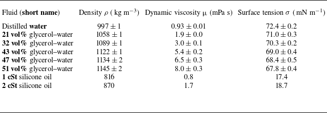
 23±1∘C
 We
We Re
Re Re=5We
 Ca=0.2
 Ca=0.105
 ut=0.15 m s−1
 un=2.45 m s−1
 ut/un=0.25
 tμ∗=2
tμ∗=2 uo=ut2+un2=2.455 m s−1
 β=tan−1(ut/un)=3.5∘
 ut=0 m s−1
 Ca=0.132
 We=345
 un=3.10 m s−1
 Ca<0.2
 ut=0.17 m s−1
 ut/un=0.23
 ut=0.26 m s−1
 ut/un=0.29
 θ
θ
 We∈[134,450]
 Re∈[940,7930]
 ±0.02 m s−1
 ut
ut ±0.01 m s−1
 un
un Ca=0.072±0.002
 rn∈[1.11,1.87]mm
 Ca
Ca rn
rn α=1/4
α=1/4 α=1/2
α=1/2 rn
rn rnαut/un
 Ca
Ca
 327pixels mm−1
 Ca=0.115±0.004
 ut=0.20±0.02 m s−1
 ut/un=0.273±0.014
 ex,p
ex,p p=m
p=m p=s
p=s
 Ca=0.213±0.002
 ut/un=0.33
 un∈[1.6,3.2] m s−1
 Ca∈[0.03,0.20]
 Ca
Ca


 Open access

