3.1. Kinematic relation for energy dissipation rate on the free surface

We first consider the mutual relations between vorticity, strain rate and divergence of the surface velocity field. The surface divergence $\mathcal {D}$ is defined as

(3.1) \begin{equation} \mathcal {D} =\nabla _{s} \cdot \boldsymbol {u} = \partial u/\partial x + \partial v/\partial y. \end{equation}

Considering the incompressibility of the fluid, $\mathcal {D}$ can also be expressed by $\mathcal {D} = - \partial w/\partial z$ . Given the no-penetration boundary condition, $w = 0$ at $z = 0$ (which is approximately valid in the present case of weak surface deformation), positive/negative divergence represents upwelling/downwelling events. The vorticity and the strain rate on the free surface are, respectively,

(3.2) \begin{equation} \omega = \nabla _{s} \times \boldsymbol {u} = \partial v/\partial x - \partial u/\partial y, \end{equation}

and

(3.3) \begin{equation} s = \sqrt {\boldsymbol {S}_{s}\boldsymbol {S}_{s}}, \end{equation}

where $\boldsymbol {S}_{s} = \left \lbrack \nabla _{s}\boldsymbol {u} + ( \nabla _{s}\boldsymbol {u} )^{T} \right \rbrack /2$ is the symmetric 2-by-2 strain-rate tensor associated with the 2-D velocity field along the surface.

To connect the surface dynamics with the local properties of turbulence, the energy dissipation rate on the free surface also examined, i.e. $\epsilon _{s} = 2\nu \left \langle \boldsymbol {SS} \right \rangle .$ Note that, here, $\boldsymbol {S} = \left \lbrack \nabla \boldsymbol {u} + ( \nabla \boldsymbol {u} )^{T} \right \rbrack /2$ is the full 3-by-3 strain-rate tensor. As $\epsilon _{s}$ is evaluated along the free surface, the boundary conditions allow significant simplifications. In particular, considering that the free surface is quasi-flat, $w$ is identically zero along the surface. This leads to $\partial w/\partial x = \partial w/\partial y = 0$ . Also, the zero-stress boundary condition imposes $\partial u/\partial z = \partial v/\partial z = 0$ . Therefore the (1, 2), (1, 3), (2, 1) and (3, 1) components of both $\nabla \boldsymbol {u}$ and $\boldsymbol {S}$ are zero. It follows that $\epsilon _{s}$ can be written as

(3.4) \begin{equation} \epsilon _{s} = 2\nu \left ( \langle \boldsymbol {S}_{s}\boldsymbol {S}_{s}\rangle + \langle \mathcal {D}^{2}\rangle \right ) = 2\nu \left ( \langle s^{2}\rangle + \langle \mathcal {D}^{2}\rangle \right ). \end{equation}

Figure 3.

(a) The comparison of turbulence energy dissipation rate on the free surface $\epsilon _{s}$ calculated based on the definition (yellow symbols), (3.8) (purple symbols) and (3.9) (blue and green symbols). (b) The joint PDF of $\partial u/\partial x$ and $\partial v/\partial y$ normalised by the Kolmogorov time scale $\tau _{\eta }$ at $Re_{\lambda } = 312$ .

We note that, in the current experiment, due to residual surfactant after skimming the surface (as mentioned above), the zero-stress boundary condition might not be strictly achieved. Therefore, $\epsilon _s$ calculated based on (3.4) might be weaker compared with a surface completely devoid of surfactants. Assessing this deviation, however, is difficult based on the surface PTV and is beyond the scope of this study. Equation (3.4) can be further expanded and rewritten as the summation of the quadratic terms of velocity gradient

(3.5) \begin{equation} \epsilon _{s} = 2\nu \left \langle 4\left ( \frac {\partial u}{\partial x} \right )^{2} + \left ( \frac {\partial u}{\partial y} \right )^{2} + 3\frac {\partial u}{\partial x}\frac {\partial v}{\partial y} \right \rangle . \end{equation}

Here, considering the properties listed in table 1, we have assumed the surface turbulence to be small-scale isotropic, which implies $\partial u/\partial x = \partial v/\partial y$ and $\partial u/\partial y = \partial v/\partial x$ , and homogeneous, which implies $\langle (\partial u/\partial x)(\partial v/\partial y)\rangle = \langle (\partial u/\partial y)(\partial v/\partial x)\rangle$ (see equation 16 in George & Hussein (Reference George and Hussein1991)). Those assumptions also allow us to write

(3.6) \begin{equation} \mathcal {D}^{2} = 2\left ( \frac {\partial u}{\partial x} \right )^{2} + 2\frac {\partial u}{\partial x}\frac {\partial v}{\partial y}, \end{equation}

(3.7) \begin{equation} \omega ^{2} = 2\left ( \frac {\partial u}{\partial y} \right )^{2} - 2\frac {\partial u}{\partial x}\frac {\partial v}{\partial y}. \end{equation}

By comparing (3.5), (3.6) and (3.7), it is evident that $\epsilon _{s}$ can be rewritten following

(3.8) \begin{equation} \epsilon _{s} = \nu \left ( 4\langle \mathcal {D}^{2}\rangle + \langle \omega ^{2}\rangle \right ). \end{equation}

This kinematic relation, which allows expression of the dissipation rate along the surface from the strength of the divergence and vorticity on it, highlights the importance of the non-solenoidal nature and surface-attached vortices to the local properties of free-surface turbulence. In the case of vanishing divergence, this relation becomes the energy dissipation rate in incompressible 2-D turbulence $\epsilon _{s} = \nu \left \langle \omega ^{2} \right \rangle$ . Equation (3.8) agrees well with the present data for all considered cases, as shown in figure 3(a). The surface dissipation rate is found to be far smaller than the bulk value $\epsilon$ . This is consistent with previous theoretical and numerical studies (Teixeira & Belcher Reference Teixeira and Belcher2000; Guo & Shen Reference Guo and Shen2010) in which a significant decrease of dissipation at the surface was found. The surface dissipation rate will be discussed further in § 3.4.

Equation (3.8) could be further simplified by assuming the compressibility ratio $\mathcal {C} = \langle ( \nabla _{s} \cdot \boldsymbol {u} )^{2}\rangle /\langle ( \nabla _{s}\boldsymbol {u} )^{2}\rangle = \langle \mathcal {D}^{2}\rangle /\langle ( \nabla _{s}\boldsymbol {u} )^{2}\rangle \approx 0.5$ as found in previous studies. Since this can also be expressed as $\mathcal {C = }\langle \mathcal {D}^{2}\rangle /\lbrack 2\langle ( \partial u/\partial x - \partial v/\partial y )^{2}\rangle \rbrack$ in the case of HIT, the condition $\mathcal {C} = 0.5$ is equivalent to a negligibly small correlation between $\partial u/\partial x$ and $\partial v/\partial y$ along the surface, i.e. $\left | \langle (\partial u/\partial x)(\partial v/\partial y)\rangle \right | \ll \langle (\partial u/\partial x)^{2}\rangle$ (Boffetta et al. Reference Boffetta, De Lillo and Gamba2004; Cressman et al. Reference Cressman, Davoudi, Goldburg and Schumacher2004). If this is assumed, the cross-product terms in (3.5), (3.6) and (3.7) are dropped and (3.8) simplifies to

(3.9) \begin{equation} \epsilon _{s} = 5\nu \langle \mathcal {D}^{2}\rangle = 5\nu \langle \omega ^{2}\rangle . \end{equation}

Figure 3(a), however, indicates that the data deviate considerably from this relationship. Indeed, the observed compressibility ratio (as reported in table 1) is much smaller than 0.5, which in turn is rooted in a strong correlation between $\partial u/\partial x$ and $\partial v/\partial y$ . This is clearly illustrated in figure 3(b), which displays the joint probability density function (PDF) of $\partial u/\partial x$ and $\partial v/\partial y$ for the case $Re_{\lambda } = 312$ , demonstrating strong anti-correlation between both quantities. This strong anti-correlation and the small compressibility ratio (as well as the weak surface divergence, which will be discussed in the following sections) might be influenced by residual surfactants on the free surface. The role of the latter, even in skimmed surface, was previously explored by Turney & Banerjee (Reference Turney and Banerjee2013). Here, and in the following, this Reynolds number will be used as exemplary case, and the behaviour of the other cases is analogous.

3.2. Divergence, vorticity and strain rate

Figure 4.

The PDFs of surface divergence $\mathcal {D}$ (panel (a)) and vorticity $\omega$ (panel (b)) at various $Re_{\lambda }$ . In both panels, darker colour represents higher $Re_{\lambda }$ and vice versa.

Here, we examine the statistical distributions of the main velocity-gradient-based quantities characterising the surface flow: divergence, vorticity and strain rate. Figure 4(a) shows the PDF of divergence $\mathcal {D}$ non-dimensionalised by $\tau _{\eta }$ for the different $Re_{\lambda }$ . The symmetric distributions indicate that the upwellings (associated with $\mathcal {D \gt }0$ ) and the downwellings ( $\mathcal {D \lt }0$ ) occur with similar frequency and strength. The long tails signal strong intermittency, as previously observed (Schumacher & Eckhardt Reference Schumacher and Eckhardt2002; Cressman et al. Reference Cressman, Davoudi, Goldburg and Schumacher2004). In addition, the approximate collapse of the PDFs for the different $Re_{\lambda }$ suggests that the statistical behaviour of the divergence follows a dissipative scaling. This is the case also for the PDFs of $\omega$ (figure 4(b)) which, however, display a far greater variance, i.e. $\langle \omega ^{2}\rangle \gg \left \langle \mathcal {D}^{2} \right \rangle .$ The relatively small magnitude of $\mathcal {D}$ is consistent with the small values of the compressibility coefficient, as discussed above. We remark that all components of the velocity-gradient tensor display symmetric distributions. This is in contrast with 3-D turbulence, where the skewness of the longitudinal velocity differences is associated with the direct energy cascade (Davidson Reference Davidson2015).

Figure 5.

(a) The PDFs of the normalised eigenvalues $\lambda _{1}$ (blue lines) and $\lambda _{2}$ (green lines) of $\boldsymbol {S}_{s}$ at various $Re_{\lambda }$ . Here, darker colour represents higher $Re_{\lambda }$ and vice versa. (b) The joint PDF of $\lambda _{1}$ and $\lambda _{2}$ for $Re_{\lambda } = 312$ .

To examine the strain rate, figure 5(a) shows the PDFs of the eigenvalues $\lambda _{1}$ and $\lambda _{2}$ of $\boldsymbol {S}_{s}$ , with $\lambda _{1} \gt \lambda _{2}$ . As $\boldsymbol {S}_{s}$ is a $2\times 2$ symmetric tensor, both $\lambda _1$ and $\lambda _2$ are real numbers. The distributions of both eigenvalues are clearly antisymmetric. We remind the reader that, in 3-D turbulence, two out of three eigenvalues tend to be positive, which indicates bi-axial stretching (Betchov Reference Betchov1956; Davidson Reference Davidson2015). Cardesa et al. (Reference Cardesa, Mistry, Gan and Dawson2013) investigated the reduced strain-rate tensor and the two associated eigenvalues along 2-D sections of 3-D turbulence, finding predominance of compression over stretching. Along the free surface, on the other hand, compression and stretching appear equally likely and intense, similarly as the instances of positive and negative divergence (see figure 4 a). The collapse of $\lambda _{1}$ and $\lambda _{2}$ for different $Re_{\lambda }$ indicates that Kolmogorov scaling again applies, as for $\mathcal {D}$ and $\omega$ . The structure of the strain field is further clarified by the joint PDF of both eigenvalues displayed in figure 5(b), the other Reynolds numbers showing analogous behaviour. The strong anti-correlation indicates a high likelihood of $\lambda _{1} \approx -\lambda _{2}$ , i.e. comparable strength of compression and stretching along perpendicular directions. This is consistent with figure 3(b) displaying relatively small surface divergence, which can be expressed as $\mathcal {D}=\lambda _{1} + \lambda _{2}$ .

Figure 6.

(a) The PDFs of normalised surface divergence square $\mathcal {D}^{2}$ , vorticity square $\omega ^{2}$ , strain-rate square $s^{2}$ and energy dissipation rate on the free surface $\epsilon _{s}$ . The dashed lines mark the scaling of power-law tails. The blue and green shaded areas illustrate the region where these quantities are smaller and larger than 10 % of their mean values, respectively. (b) The PDFs of two components of the velocity-gradient tensor $\partial u/\partial x$ (yellow symbols) and $\partial u/\partial y$ (blue symbols) normalised by their r.m.s. The solid lines show the fitted Gaussian distribution. The red shaded area from –0.3 to 0.3 marks the region where the PDFs are approximately Gaussian.

The magnitude of the different quantities is compared in figure 6(a), showing the PDFs of $\mathcal {D}^{2}$ , $\omega ^{2}$ , $s^{2}$ and $\epsilon _{s}$ , normalised by their mean value. In the range of low intensity events (blue shaded area), the distributions show power-law scaling with slopes of $1/2$ for $s^{2}$ and $\epsilon _{s}$ , and $- 1/2$ for $\mathcal {D}^{2}$ and $\omega ^{2}$ . Power-law tails over the small-magnitude range were also observed for PDFs of squared vorticity and strain rate in 3-D turbulence by Yeung et al. (Reference Yeung, Donzis and Sreenivasan2012) and Carter & Coletti (Reference Carter and Coletti2018), who explained them by the ansatz that small-velocity-gradient events behave as random variables. This is also the case here, as illustrated by figure 6(b), where PDFs of $\partial u/\partial x$ and $\partial u/\partial y$ are shown. It is evident that both quantities (and other components of the velocity gradient, not shown) approximately follow a Gaussian distribution when their magnitude is relatively small, e.g. less than 30 % of their r.m.s. values, as indicated in figure 6(b). As the quantities in figure 6(a) are summation of squares of velocity-gradient components, we expect them to follow chi-square distributions

(3.10) \begin{equation} P(X) \sim X^{k/2 - 1}e^{- X/2}, \end{equation}

where $X$ is the variable representing $\mathcal {D}^{2}$ , $\omega ^{2}$ , $s^{2}$ , and $\epsilon _{s}$ , $k$ is the order of the chi-square distribution specifying the number of independent squared terms being summed and $e$ is the natural exponent. For small $X$ , this yields a power-law tail with a slope of $k/2 - 1$ . For $\mathcal {D}^{2}$ and $\omega ^{2}$ , only one squared term is involved with $k = 1$ , and the power-law slope $- 1/2$ is retrieved. The squared strain rate can be written as $s^{2} = (\partial u/\partial x)^{2} + (\partial v/\partial y)^{2} + (\partial u/\partial y + \partial v/\partial x)^{2}/2$ , hence $k = 3$ , which yields the observed $1/2$ slope. Finally, the surface dissipation can be expressed by $\epsilon _{s} = 2\nu \left \lbrack s^{2} + (\partial w/\partial z)^{2} \right \rbrack$ , where $\partial w/\partial z$ is not an independent term considering the incompressibility condition. Therefore, $k = 3$ is again obtained, and the scaling of the low-range tail of $\epsilon _{s}$ follows the one of $s^{2}$ .

At the opposite end (green shaded area in figure 6 a), we notice that the right tails of the PDFs of $\omega ^{2}$ and $s^{2}$ follow similar patterns. This was also observed in 3-D turbulence (Yeung et al. Reference Yeung, Donzis and Sreenivasan2012), suggesting that intense events of strain and vorticity are concurrent. The distribution of $\epsilon _{s}$ essentially matches that of $s^{2}$ , consistent with (3.4) which results in $\epsilon _{s} \approx 2\nu s^{2}$ for $\mathcal {C} \ll 1$ . Although the divergence is in general relatively small, its intermittency is even higher than the other analysed quantities. The overall strong intermittency of the velocity gradient as well as its associated quantities on the free surface was recently found to be associated with the nonlinear self-amplification of the velocity gradient (Qi et al. Reference Qi, Xu and Coletti2025), which also accounts for the strong intermittency in 3-D turbulent flows (Meneveau Reference Meneveau2011; Johnson & Wilczek Reference Johnson and Wilczek2024).

3.3. Topology of small-scale structures

Figure 7.

(a) The number of high-intensity objects found in the FOV as a function of thresholds. (b) The PDFs of the normalised area of high-intensity objects. The dashed line marks the power-law scaling of $- 2$ . (c) The PDFs of the aspect ratio of high-intensity events. In all of the panels, the purple, green and blue symbols represent high-divergence, high-vorticity and high-strain objects, respectively. Only the data for $Re_{\lambda } = 312$ are included.

We then examine the topology of small-scale structures; in particular, three sets of discrete structures used to characterise the spatial organisation of events of high surface divergence, vorticity and strain rate. Those structures are defined as contiguous regions satisfying the conditions $\left | \mathcal {D} \right | \gt \alpha _{\mathcal {D}}{\langle \mathcal {D}^{2}\rangle }^{1/2}$ , $|\omega | \gt \alpha _{\omega }{\langle \omega ^{2}\rangle }^{1/2}$ and $s \gt \alpha _{s}\langle s\rangle$ , where $\alpha _{\mathcal {D}}$ , $\alpha _{\omega }$ and $\alpha _{s}$ are positive constants. To determine appropriate thresholds, we analyse the percolation behaviour of the intense structures as first proposed by Moisy & Jiménez (Reference Moisy and Jiménez2004). For high threshold values, only a few small objects can be detected. As the threshold decreases, the objects grow in size and number and eventually start merging. The optimal threshold is obtained by identifying the intermediate value for which the objects are most numerous. This procedure was used extensively to identify structures in various configurations including channel flows (Lozano-Durán et al. Reference Lozano-Durán, Flores and Jiménez2012), free shear flows (Dong et al. Reference Dong, Lozano-Durán, Sekimoto and Jiménez2017) and homogeneous turbulence (Carter & Coletti Reference Carter and Coletti2018).

Here, the velocity gradient measured at the position of each particle is first interpolated on a Cartesian grid with size equal to half the mean inter-particle distance. Figure 7(a) then shows how the number of detected objects varies as a function of threshold level, yielding the choice $\alpha _{\mathcal {D}} = 0.4$ , $\alpha _{\omega } = 0.6$ and $\alpha _{s} = 1.5$ . It is noted that the following results are not sensitive to the exact values of thresholds. Moreover, objects that touch the FOV boundary are discarded. Although this may lead to underestimation of the number of large structures, it will be shown that the vast majority of the identified objects are much smaller than the FOV.

Figure 7(b) shows the PDFs of the area of high-divergence, high-vorticity and high-strain-rate structures, normalised by the Kolmogorov scale. The size of the structures is widely distributed over four decades. The high-vorticity and high-strain objects follow a similar trend, confirming the correlation between events of intense $\omega$ and $s$ . These structures are on average larger compared with the regions of high divergence. Over some size range, the distributions appear compatible with a power-law decay, which may suggest a link with the scale-invariant properties of turbulence (Sreenivasan Reference Sreenivasan1991; Moisy & Jiménez Reference Moisy and Jiménez2004; Carter & Coletti Reference Carter and Coletti2018). The limited range of scales over which this is evident, however, does not allow any conclusive statement in this sense.

In order to characterise the geometry of these structure, we also consider their aspect ratio $\text {AR} = R_{1}/R_{2}$ , where $R_{1}$ and $R_{2}$ are the major and minor axes of an ellipse that has the same second central moments as the structure. To ensure an accurate AR calculation, objects with area smaller than 5 grid cells (corresponding to around $5\eta ^{2}$ ) are not considered in these statistics. It is found the results do not display discernible dependence on the cutoff value between 3 and 9 grid cells. Figure 7(c) shows the PDFs of AR for the three types of structures. Again, the curves for the high-vorticity and high-strain objects largely overlap. Those structures have generally larger AR, indicating that high-vorticity and high-strain-rate structures are more elongated compared with those of high divergence.

Figure 8.

(a–c) Snapshots of surface divergence field (a), vorticity field (b) and strain field (c) on the free surface $Re_{\lambda } = 312$ . (d) Overlap coefficients as a function of $Re_{\lambda }$ . The purple, green and blue symbols represent divergence–vorticity, divergence–strain and vorticity–strain overlap, respectively.

These properties are confirmed by the visual observations of instantaneous fields, samples of which are reported in figure 8(a–c): the high-divergence events are relatively small scale and spotty whereas the high-vorticity and high-strain regions are larger and more elongated. This divergence snapshot is consistent with the numerical simulation at a lower Reynolds number ( $Re_T\approx 1800$ ) by Herlina & Wissink (Reference Herlina and Wissink2019), in which the surface divergence also appears to have a smaller length scale compared with the integral scale in the bulk. Moreover, the vorticity and strain-rate fields follow similar patterns, with high-vorticity magnitude (both positive and negative) events also overlapping with high-strain regions. This concurrence of intense vorticity and strain is also found in 3-D turbulence (Yeung et al. Reference Yeung, Zhai and Sreenivasan2015). To quantify the topological connection between such objects, we define the overlapping coefficients between $\mathcal {D}$ , $\omega$ and $s$ , based on a procedure similar to the one used by Berk & Coletti (Reference Berk and Coletti2023). For example, the overlap between high-vorticity and high-divergence structures is characterised by

(3.11) \begin{equation} R_{\mathcal {D}\omega } = \frac {A_{FOV}\langle A_{\mathcal {D}\omega }\rangle }{\langle A_{\mathcal {D}}A_{\omega }\rangle }, \end{equation}

where $A_{FOV}$ is the total area of the FOV. Here, $A_{\mathcal {D}}$ and $A_{\omega }$ are the area of high-divergence and high-vorticity regions, respectively and $A_{\mathcal {D}\omega }$ denotes the overlapping area between these regions. If both types of structures are spatially uncorrelated, $R_{\mathcal {D}\omega } = 1$ . Similarly, the divergence/strain-rate and vorticity/strain-rate overlapping coefficients are defined as

(3.12) \begin{align} R_{\mathcal {D}s} = \frac {A_{FOV}\langle A_{\mathcal {D}s}\rangle }{\langle A_{\mathcal {D}}A_{s}\rangle },\end{align}

(3.13) \begin{align} R_{\omega s} = \frac {A_{FOV}\langle A_{\omega s}\rangle }{\langle A_{\omega }A_{s}\rangle },\end{align}

where $A_{s}$ represents the area of high-strain structures, and $A_{\mathcal {D}s}$ and $A_{\omega s}$ are overlapping areas defined similarly. Figure 8(d) shows $R_{\mathcal {D}\omega }$ , $R_{\mathcal {D}s}$ and $R_{\omega s}$ for the different $Re_{\lambda }$ . In all cases, high-vorticity and high-strain structures show significant correlation, consistent with the previous observations. Here, $R_{\mathcal {D}\omega }$ and $R_{\mathcal {D}s}$ are much weaker than $R_{\omega s}$ , but the high-divergence events are more likely to be concurrent with high strain rate than high vorticity.

3.4. Second-order velocity structure functions

Figure 9.

(a) The longitudinal second-order structure function $D_{LL}$ as a function of the separation distance. The dashed line denotes $2/3$ power-law scaling. (b) Value of $D_{LL}$ normalised by $(r\epsilon )^{2/3}$ . (c) Value of $D_{LL}$ normalised by $( r\epsilon _{s} )^{2/3}$ . The orange dashed line marks $C_{2s} \approx 3.5$ . In all of the panels, the darker colour represents high $Re_{\lambda }$ and vice versa. The green shaded area marks the inertial range.

After exploring the small-scale properties of the surface flow field, we consider how the turbulent kinetic energy is distributed across the spatial scales as described by the second-order longitudinal structure function. This is defined as

(3.14) \begin{equation} D_{LL} = \left \langle \left (u_{r}\left ( \boldsymbol {x} + r{\hat {\boldsymbol {e}}}_{r} \right ) - u_{r}\left ( \boldsymbol {x} \right )\right )^{2} \right \rangle , \end{equation}

where $r$ is the separation distance, ${\hat {\boldsymbol {e}}}_{r}$ represents the unit vector along the separation and $u_{r}$ is the velocity component in the same direction. Figure 9(a) shows $D_{LL}$ as a function of $r/\eta$ for the different $Re_{\lambda }$ . In all cases, a clear scaling $D_{LL} \sim r^{2/3}$ is visible for $r/\eta \gt 20$ , consistent with the classic theory of Kolmogorov (Reference Kolmogorov1941) in the inertial sub-range. This was also observed in the laboratory experiments by Goldburg et al. (Reference Goldburg, Cressman, Vörös, Eckhardt and Schumacher2001) and Cressman et al. (Reference Cressman, Davoudi, Goldburg and Schumacher2004), and in outdoor water streams by Chickadel et al. (Reference Chickadel, Talke, Horner-Devine and Jessup2011) (who reported the equivalent scaling of the energy spectrum with $k^{- 5/3}$ , $k$ being the wavenumber) and by Sanness Salmon et al. (Reference Salmon, Henri, Baker, Kozarek and Coletti2023).

At smaller separations, the structure functions do not transition to the scaling $D_{LL}\sim r^{2}$ expected for smooth flows in the dissipation range, and instead their slopes become much shallower than in the inertial sub-range. This behaviour was recently reported by Li et al. (Reference Li, Wang, Qi and Coletti2024) using much sparser particle concentrations. Here, the finer spatial resolution allows us not only to confirm this finding, but also to reveal that the anomalously large relative velocities persist down to millimetric separations. As discussed in Li et al. (Reference Li, Wang, Qi and Coletti2024), this behaviour is similar to the formation of caustics in the velocity fields described by inertial particles in turbulence: such fields are also compressible, with intermittently large relative velocities and thus anomalous scaling exponents of the structure functions at small scales (Bec et al. Reference Bechlars and Sandberg2010; Bewley et al. Reference Bewley, Saw and Bodenschatz2013; Berk & Coletti Reference Berk and Coletti2021; Bec et al. Reference Bec, Gustavsson and Mehlig2024). We note that, as the floating particles follow the fluid motion, their relative velocity must ultimately recover the scaling $u_{r} \sim r$ (and thus $D_{LL} \sim r^{2}$ ) in the limit of vanishing separations. This, however, may happen at scales only slightly larger than the particle diameter, not accessible even in the present high-resolution imaging system.

Besides the scaling with the separation $r$ , a crucial prediction of Kolmogorov’s theory is the dependence of the structure function with the dissipation in the inertial sub-range. In 3-D turbulence, the theory predicts $D_{LL} = C_{2}(\epsilon r)^{2/3}$ , where $C_{2} \approx 2.1$ is the Kolmogorov constant (Sreenivasan Reference Sreenivasan1995). The compensated plots $D_{LL}/(\epsilon r)^{2/3}$ in figure 9(b) show that this relation does not hold in free-surface turbulence: the lines are not close to the value of 2.1 in the inertial range and, more importantly, they do not collapse. In fact, the dynamics on the free surface expected to be determined by the energy dissipation rate on the free surface $\epsilon _{s}$ rather than by the one in the bulk water $\epsilon$ . Indeed, the compensated plots $D_{LL}/ ( \epsilon _{s}r )^{2/3}$ in figure 9(c) show a much better collapse which indicates that the classic scaling still holds for free-surface turbulence when the dissipation rate on the surface is considered, i.e. $D_{LL} = C_{2s} ( \epsilon _{s}r )^{2/3}$ . Here, a distinct factor $C_{2s} \approx 3.5$ is obtained.

3.5. Scales of surface divergence, vorticity and strain rate

Figure 10.

The Eulerian autocorrelation functions of divergence (a), vorticity (b) and strain (c) at different $Re_{\lambda }$ . In all of the panels, the darker colour represents higher $Re_{\lambda }$ .

As seen in § 3.3, the surface divergence, vorticity and strain rate exhibit different length scales. This aspect is further investigated by examining the spatial autocorrelation functions of each quantity

(3.15) \begin{align} \rho _{\mathcal {D}}^{E} = \frac {\langle \mathcal {D}'\left ( \boldsymbol {x} \right )\mathcal {D}'\left ( \boldsymbol {x} + r\hat {\boldsymbol {e}}_{r} \right )\rangle }{\langle \mathcal {D}'^{2}\rangle }, \end{align}

(3.16) \begin{align} \rho _{\omega }^{E} = \frac {\langle \omega '\left ( \boldsymbol {x} \right )\omega '\left ( \boldsymbol {x} + r{\hat {\boldsymbol {e}}}_{r} \right )\rangle }{\langle \omega '^{2}\rangle },\end{align}

(3.17) \begin{align} \rho _{s}^{E} = \frac {\langle s'\left ( \boldsymbol {x} \right )s'\left ( \boldsymbol {x} + r{\hat {\boldsymbol {e}}}_{r} \right )\rangle }{\langle s'^{2}\rangle },\end{align}

where the superscript $E$ stands for Eulerian and the prime denotes fluctuations around the ensemble average. Figure 10 shows the autocorrelation for the various $Re_{\lambda }$ . The divergence field (figure 10 a) exhibits a characteristic length scale around (5–10) $\eta$ , while the vorticity and strain-rate fields are characterised by somewhat larger correlation scales $\sim 20\eta$ and $\sim 30\eta$ , respectively. This observation is consistent with the result in figures 7(b) and 8. Beyond some experimental scatter, the autocorrelation functions show no discernible dependence on $Re_{\lambda }$ , with Kolmogorov scaling providing a fair collapse of the curves.

As the velocity gradient is obtained along floating particle trajectories, the temporal scales can also be investigated by calculating the temporal autocorrelation functions of divergence, vorticity and strain rate, respectively,

(3.18) \begin{align} \rho _{\mathcal {D}}^{L} = \frac {\mathcal {\langle D'}(t)\mathcal {D'}(t + \tau )\rangle }{\mathcal {\langle D}'^{2}\rangle },\end{align}

(3.19) \begin{align} \rho _{\omega }^{L} = \frac {\langle \omega '(t)\omega '(t + \tau )\rangle }{\langle \omega '^{2}\rangle },\end{align}

(3.20) \begin{align} \rho _{s}^{L} = \frac {\langle s'(t)s'(t + \tau )\rangle }{\langle s'^{2}\rangle }.\end{align}

Here, the superscript $L$ stands for Lagrangian, $t$ represents the generic temporal abscissa and $\tau$ is the time delay. Figure 11 shows the temporal autocorrelation functions for the different $Re_{\lambda }$ , with the Kolmogorov scaling that again provides a reasonable collapse of the curves. The surface divergence shows a time scale comparable to $\tau _{\eta }$ , confirming it is driven by small-scale processes. On the other hand, the time scales of both vorticity and strain rate are significantly larger and comparable to the integral time scale, suggesting that surface-attached vortices and surface-parallel stretching and compression are long-lived compared with the lifetime of sources and sinks. These time scales, in fact, are also larger than their characteristic time scales in 3-D turbulence, which are expected to scale with $\tau _{\eta }$ .

Figure 11.

The Lagrangian autocorrelation functions of divergence (a), vorticity (b) and strain (c) at different $Re_\lambda$ . In all of the panels, the darker colour represents higher $Re_{\lambda }$ .

Figure 12.

(a) The Eulerian autocorrelation functions for positive divergence (purple line) and negative divergence (green line). (b) The Lagrangian autocorrelation functions for positive divergence (purple line) and negative divergence (green line).

Given the importance of the imbalance between upwellings and downwellings (Perot & Moin Reference Perot and Moin1995; Guo & Shen Reference Guo and Shen2010; Ruth & Coletti Reference Ruth and Coletti2024), it is useful to distinguish between the scales associated with both types of events. Figures 12(a) and 12(b) plot the Eulerian and Lagrangian autocorrelation functions $\rho _{\mathcal {D}}^{E}$ and $\rho _{\mathcal {D}}^{L}$ , respectively, conditioning on $\mathcal {D} \gt 0$ and $\mathcal {D} \lt 0$ . It is clear that upwellings are associated with larger spatial and temporal scales along the surface flow compared with downwellings. This is consistent with the observation by Ruth & Coletti (Reference Ruth and Coletti2024) in the same facility and by Guo & Shen (Reference Guo and Shen2010) based on numerical simulations.

3.6. Cross-correlation among divergence, vorticity and strain rate

Figure 13.

(a) The Eulerian cross-correlation functions between divergence and vorticity magnitude at different $Re_{\lambda }$ . (b) The Lagrangian cross-correlation function between divergence and vorticity magnitude at different $Re_{\lambda }$ . This panel shares the same legend with panel (a). The yellow shaded area marks the vortex-stretching process, and the green shaded area marks the diffusion process of surface-attached vortices. The schematic illustrates the vortex-stretching process. The green spiral marks the surface-attached vortex, the red arrows represent the negative divergence, and the blue plane shows the free surface.

Having characterised the spatial and temporal scales of divergence, vorticity and strain rate of the surface flow, we investigate its dynamics by considering the mutual correlation between those quantities, which will prove insightful towards a mechanistic understanding of the processes. We first consider the Eulerian cross-correlation between divergence and vorticity $\rho _{\mathcal {D}|\omega |}^{E}$

(3.21) \begin{equation} \rho _{\mathcal {D}|\omega |}^{E} = \frac {\langle \mathcal {D}'\left ( \boldsymbol {x} \right )|\omega |'\left ( \boldsymbol {x} + r{\hat {\boldsymbol {e}}}_{r} \right )\rangle }{ \mathcal {\langle D}'^{2}\rangle ^{1/2}\langle |\omega |'^{2}\rangle ^{1/2} }, \end{equation}

where the absolute value of the vorticity is used as the rotational direction of surface-attached vortices is immaterial. Figure 13(a) shows the cross-correlation for various $Re_{\lambda }$ , with Kolmogorov scaling providing again a fair collapse of the different curves. For all cases, $\rho _{\mathcal {D}|\omega |}^{E} \approx - 0.03$ at $r = 0$ is observed. This suggests that, although the correlation between these two quantities is weak, strong vorticity is more likely to be associated with negative surface divergence; i.e. surface-attached vortices are stronger when downwelling events occur. Moreover, figure 13(a) indicates a characteristic correlation scale $\approx 10\eta$ . This is close to the length scale of the divergence as the latter decorrelates from itself faster than the vorticity (see figure 10).

To further probe the interaction between divergence and vorticity, we also examine the Lagrangian cross-correlation, which is defined as

(3.22) \begin{equation} \rho _{\mathcal {D}|\omega |}^{L} = \frac {\mathcal {\langle D'}(t)|\omega |'(t + \tau )\rangle }{\mathcal {\langle D}'^{2}\rangle ^{1/2}\langle |\omega |'^{2}\rangle ^{1/2}}. \end{equation}

As shown in figure 13(b), this cross-correlation remains around zero before $\tau \lt 0$ , suggesting that strong vorticity events do not affect the divergence at later times. However, for $\tau \geqslant 0$ , $\rho _{\mathcal {D}|\omega |}^{L}$ becomes negative and dips during a few Kolmogorov time units. This anti-correlation between $\mathcal {D}$ and $\omega$ , corroborating the observation in figure 13(a), indicates that sinks in the surface flow are statistically associated with the enhancement of surface-attached vortices at a later time. This can be explained by considering the physical picture illustrated in the inset of figure 13(b): when a sink (marked by a red arrow) is formed, the correspondent downwelling flow stretches downwards surface-attached vortex filaments (marked as a green spiral). As a result, the vorticity magnitude grows and $\rho _{\mathcal {D}|\omega |}^{L}$ decreases significantly (yellow shaded area in the plot). The typical duration of the vortex stretching, around $2\tau _{\eta }$ , is consistent with the time scale of the events of negative divergence highlighted in figure 12(b). When the surface sink has dissipated, the vorticity diffuses and $\rho _{\mathcal {D}|\omega |}^{L}$ approaches zero (blue shaded area). We note that this picture should hold for different $Re_{\lambda }$ , as indicated by the good collapse of the lines in figure 13(b).

Figure 14.

(a) The spatial-temporal cross-correlation between the divergence and vorticity magnitude as a function of separation distance. The colours represent the time delay $\tau$ . (b) The PDFs of the vortex-stretching term. The darker colour represent the higher $Re_{\lambda }$ .

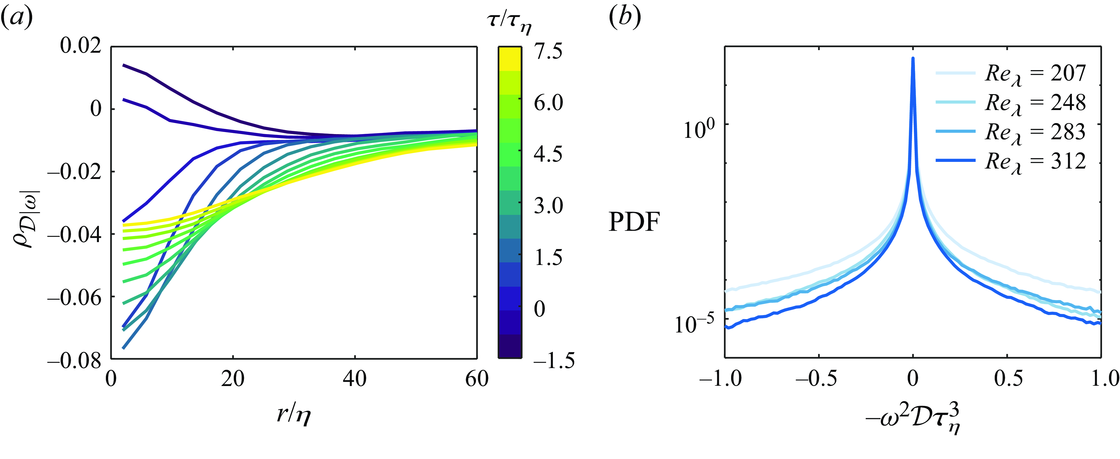
This picture of the connection between vortex stretching and surface divergence is corroborated by figure 14(a), plotting the spatio-temporal cross-correlation between the divergence and vorticity

(3.23) \begin{equation} \rho _{\mathcal {D}|\omega |} = \frac {\mathcal {\langle D'}\left ( \boldsymbol {x},t \right )|\omega |'\left ( \boldsymbol {x} + r{\hat {\boldsymbol {e}}}_{r},t + \tau \right )\rangle }{\mathcal {\langle D}'^{2}\rangle ^{1/2}\langle |\omega |'^{2}\rangle ^{1/2}}. \end{equation}

The cross-correlation is again weak for $\tau \lt 0$ ; whereas, during the initial stage of the downwelling ( $0 \lt \tau \lt 2\tau _{\eta }$ ), the vorticity intensifies and the cross-correlation dips into the negative range. The anti-correlation extends spatially to $r \approx 10\eta$ , i.e. the characteristic length scale of the divergence; while after $\tau \gt 2\tau _{\eta }$ , when the sink dissipates, the diffusion of the vorticity leads to an increase of the cross-correlation length scale.

The connection between the surface divergence and surface-attached vortices has been explored by several authors. Banerjee (Reference Banerjee1994) proposed that a correlation must exist between the surface divergence and the number of surface-attached vortices, which was recently demonstrated by Babiker et al. (Reference Babiker, Bjerkebæk, Xuan, Shen and Ellingsen2023). Shen et al. (Reference Shen, Zhang, Yue and Triantafyllou1999) used numerical simulations to provide a mechanistic interpretation of such correlation, showing how upwellings bring hairpin vortices close to the surface, where their surface-parallel section is dissipated, leaving vortex filaments that connect to the surface. The present analysis has emphasised the relation between surface vortices and downwellings, rather than upwellings. The former are naturally associated with vortex stretching, which in turn is classically attributed a key role in the energy cascade. However, the picture appears to be the completely different in free-surface turbulence, as we now show.

The evolution of vorticity under the action of the strain field is often characterised by examining the vortex-stretching term $\boldsymbol {\omega } \cdot \boldsymbol {S} \cdot \boldsymbol {\omega }$ in the enstrophy transport equation, where $\boldsymbol {\omega }$ is the vorticity vector. On the free surface, this term reduces to $\omega ^{2}(\partial w/\partial z) = - \omega ^{2}\mathcal {D}$ . Figure 14(b) shows the PDF of this terms normalised by Kolmogorov scales for all $Re_{\lambda }$ . The distribution is symmetric and strongly intermittent. The symmetry is in stark contrast with the behaviour of 3-D turbulence, in which vortex stretching is predominant (Mullin & Dahm Reference Mullin and Dahm2006; Buxton & Ganapathisubramani Reference Buxton and Ganapathisubramani2010; Bechlars & Sandberg Reference Bechlars and Sandberg2017). The fact that the free surface ts to suppress the vortex stretching is also observed in Qi et al. (Reference Qi, Xu and Coletti2025) by examining the asymmetry of the joint PDF of velocity-gradient invariants. This result may provide clues regarding the energy cascade along the free surface, which has been found to show inverse energy transfer from small to large scales (Pan & Banerjee Reference Pan and Banerjee1995; Lovecchio et al. Reference Lovecchio, Zonta and Soldati2015).

Figure 15.

(a) The Eulerian cross-correlation function for the divergence and the larger eigenvalue of the strain-rate tensor on the surface $\lambda _{1}$ for different $Re_{\lambda }$ . This panel shares the same legend with panel (b). The inset illustrates the relation between the positive/negative divergence (red arrows) and the strength of stretching (yellow arrows) and compression (green arrows) on the free surface. The length of the arrows marks the magnitude of stretching and compression. (b) The Lagrangian cross-correlation for the divergence and $\lambda _{1}$ for different $Re_{\lambda }$ . The green shaded area which covers a time scale of $10\tau _{\eta }$ marks the time range when $\lambda _{1}$ increases and decreases.

As shown in § 3.3, the surface divergence is associated with vorticity as well as with strain rate, and in fact somewhat more significantly with the latter. To quantify this aspect, we consider the Eulerian cross-correlation between the surface divergence and $\lambda _{1}$

(3.24) \begin{equation} \rho _{\mathcal {D}\lambda _{1}}^{E} = \frac {\langle \mathcal {D}'\left ( \boldsymbol {x} \right )\lambda _{1}'\left ( \boldsymbol {x} + r{\hat {\boldsymbol {e}}}_{r} \right )\rangle }{\mathcal {\langle D}'^{2}\rangle ^{1/2}\langle \lambda _{1}'^{2}\rangle ^{1/2} }. \end{equation}

Figure 15(a) plots this quantity for all cases, showing a positive correlation. This indicates that a larger positive surface divergence (stronger source) is likely to be associated with large (i.e. above average) strain rate along the surface stretching direction. As $\lambda _{1}$ and $\lambda _{2}$ are highly anti-correlated (see figure 5 b), a compression of comparable magnitude is also likely to occur in the surface-parallel direction perpendicular to the one of stretching (with the compression slightly weaker than the stretching to satisfy incompressibility). This flow pattern is illustrated by the upper schematic in figure 15(a). On the other hand, a negative divergence is likely associated with weak (i.e. below average) strain rate along the surface accompanied by a weak compression perpendicular to it, as also sketched in the lower schematic of figure 15(a). The cross-correlation has a characteristic scale comparable to the length scale of divergence, similar as $\rho _{\mathcal {D}|\omega |}^{E}$ (figure 13 a), although the magnitude of $\rho _{\mathcal {D}\lambda _{1}}^{E}$ is somewhat larger. This is consistent with the observation that divergent regions overlap slightly more with high-strain-rate regions compared with high-vorticity regions (figure 7 d).

Finally, we examine the Lagrangian cross-correlation between divergence and $\lambda _{1}$ (figure 15 b)

(3.25) \begin{equation} \rho _{\mathcal {D}\lambda _{1}}^{L} = \frac {\langle \mathcal {D}'(t)\lambda _{1}'(t + \tau )\rangle }{\mathcal {\langle D}'^{2}\rangle ^{1/2}\langle \lambda _{1}'^{2}\rangle ^{1/2}}. \end{equation}

Before a strong divergence event occurs (i.e. $\tau \lt 0$ ), $\mathcal {D}$ and $\lambda _{1}$ grow together, as indicated by the increasing correlation $\rho _{\mathcal {D}\lambda _{1}}^{L}$ . Considering the strong anti-correlation between $\lambda _{1}$ and $\lambda _{2}$ , this implies that the formation of a source is preceded by an increase in magnitude of the stretching–compression saddle along the surface. After $\lambda _{1}$ reaches its maximum at $\tau = 0$ , it decreases and slowly approaches its mean with the stretching–compression saddle recovering to its average magnitude. For all $Re_{\lambda }$ , the duration of significant correlation is approximately $10\tau _{\eta }$ (green shaded area), which is consistent with the lifetime of high-strain-rate events (figure 11 c).

3.7. Clustering on the free surface

We finally examine the clustering of the floating particles along the surface. This process, originating from the compressible nature of the free surface, differs from the clustering of inertial particles in incompressible turbulence (Balachandar & Eaton Reference Balachandar and Eaton2010; Brandt & Coletti Reference Brandt and Coletti2022). The latter results from the fact that inertial particles depart from the pathlines of fluid parcels whose fluctuations they cannot follow, thus leading to a compressible field (Maxey Reference Maxey1987). On the other hand, floating particles cannot follow the surface pathlines entering the bulk.

Figure 16(a) shows the radial distribution function (RDF) of floating particles defined as $g(r) = ( N_{r}/A_{r} )/ ( N_{t}/A_{FOV} )$ , where $N_{r}$ is the number of particles within a narrow circular ring with radius $r$ and area $A_{r}$ , and $N_{t}$ is the total number of particles in the FOV. The RDF quantifies the local concentration around a generic particle, and thus values larger than unity indicate the formation of clusters over a certain length scale. In the present case, the values indicate moderate degree of clustering. This is compatible with the weak compressibility we observe. An exponential fit to the data yields a characteristic length scale of the clustering around $30\eta$ , close to the length scale $\sim 20\eta$ found in the simulations by Schumacher & Eckhardt (Reference Schumacher and Eckhardt2002). The fact that the cluster length scale is significantly larger than that of divergence (figure 10 a) suggests the clustering is also affected by the large-scale motion on the free surface. The inset of figure 16(a) displays the same RDF in logarithmic scale. While the range is not sufficient for a conclusive statement, the data are compatible with a power-law decay, which would indicate spatial self-similarity of the concentration field. This would be in turn consistent with previous works that show how floating particles cluster over fractal sets (Boffetta et al. Reference Boffetta, Davoudi and Lillo2006; Larkin et al. Reference Larkin, Bandi, Pumir and Goldburg2009).

The clustering of floating particles is also characterised using the Voronoi tessellation method (Monchaux et al. Reference Monchaux, Bourgoin and Cartellier2010). Figure 16(b) displays the PDF of the area of the Voronoi cells $A_{V}$ for $Re_{\lambda } = 312$ , compared with the PDF that approximates the distribution of scattered particles in a random Poisson process (Ferenc & Néda Reference Ferenc and Néda2007). We note the data only cover a limited range down to $A_{V}/\left \langle A_{V} \right \rangle \approx 0.3$ . This corresponds to $5 \times 5$ pixels in raw images, slightly larger than the particle size. Voronoi cells smaller than this criterion tend to have larger uncertainty. Nevertheless, the area PDF clearly shows higher probability at $A_{V}/\left \langle A_{V} \right \rangle \lt 0.83$ and $A_{V}/\left \langle A_{V} \right \rangle \gt 2$ , indicating the occurrence of clusters and voids, respectively. The degree of clustering is quantified by calculating the standard deviation of the PDF, $\sigma _{AV}$ , and comparing with that of the random Poisson process, $\sigma _{rpp} \sim 0.53$ . The ratio $\sigma _{AV}/\sigma _{rpp} \sim 1.6$ confirms the moderate intensity of the clustering.

Figure 16.

(a) The RDF of floating particles on the free surface for various $Re_{\lambda }$ . The inset shows the same figure with the horizontal and vertical axes in logarithmic scales. This panel shares the same legend with panel (c). (b) The PDF of the area of Voronoi cells around floating particles for the case $Re_{\lambda } = 312$ . The purple line shows the PDF for a random Poisson process. The black dashed line at $A_{V}/\langle A_{V} \rangle = 0.83$ marks the crossing point between both curves. (c) The Lagrangian autocorrelation of the partile concentration for various $Re_{\lambda }$ .

The time scale of the clustering is further characterised by calculating its Lagrangian autocorrelation function

(3.26) \begin{equation} \rho _{C_{V}}^{L} = \frac {\langle C_{V}'(t)C_{V}'(t + \tau )\rangle }{\langle C_{V}'^{2}\rangle }, \end{equation}

as shown in figure 16(c), where $C_{V} = 1/A_{V}$ denotes the local concentration of particles. Results for different $Re_{\lambda }$ collapse and exhibit a similar time scale around $\sim 40\tau _{\eta }$ . This is significantly larger than the characteristic time scale of the divergence and is close to the integral time scale, highlighting again the role of the large-scale motions. This result is consistent with the observation by Lovecchio et al. (Reference Lovecchio, Marchioli and Soldati2013), who reported clusters evolving over a time scale similar to and even larger than the integral time scale of the underlying turbulence.

It is worth mentioning that, although the formation of clusters is associated with the compressible surface velocity field, the distribution of clusters is not expected to exhibit a strong connection with the instantaneous divergence field. Instead, clusters (voids) emerge where persistent sinks (sources) are present, i.e. the time history of the surface divergence needs to be considered. This mechanism potentially elucidates the distinct temporal and spatial scales exhibited by the clusters compared with the divergence.