





1. Introduction
Turbulence is a strongly nonlinear phenomenon exhibiting chaotic spatiotemporal behaviour at many scales. Despite its complexity, a certain degree of coherence is observed and has been studied for many years with the goal of describing dynamics of turbulent flows in terms of a few coherent structures (Jiménez Reference Jiménez2018a). In the context of wall-bounded flows, a considerable amount of research (see e.g. Hamilton, Kim & Waleffe Reference Hamilton, Kim and Waleffe1995; Waleffe Reference Waleffe1997; Jiménez & Pinelli Reference Jiménez and Pinelli1999; Schoppa & Hussain Reference Schoppa and Hussain2002) is devoted to understanding the turbulence-sustaining mechanisms in terms of quasi-streamwise vortices, i.e. coherent regions of vortically moving fluid transverse to the flow direction, and streaks, i.e. elongated high- or low-speed modulation of the base flow. Despite the abundant numerical and experimental evidence supporting the importance of streaks in wall turbulence, and the intuitive physical picture provided by their interactions with vortices, the definition of a streak is based on experimental observations, thus is inherently subjective (Jiménez Reference Jiménez2018b). Consequently, one does not know how much is lost by neglecting the rest of the fluctuations in turbulent flow.
A complementary, yet mathematically exact, approach to low dimensionality in turbulence is provided by the so-called (Waleffe Reference Waleffe2001) exact coherent structures (ECS), which are unstable time-invariant (self-sustaining) solutions of the Navier–Stokes equations such as equilibria, travelling waves and periodic orbits. These correspond to compact low-dimensional objects in the infinite-dimensional state space of all possible flow fields, and influence the dynamics in their vicinity via their stable and unstable manifolds (Gibson, Halcrow & Cvitanović Reference Gibson, Halcrow and Cvitanović2008; van Veen & Kawahara Reference van Veen and Kawahara2011; Budanur et al. Reference Budanur, Short, Farazmand, Willis and Cvitanović2017; Budanur & Hof Reference Budanur and Hof2018; Budanur, Dogra & Hof Reference Budanur, Dogra and Hof2019; Farano et al. Reference Farano, Cherubini, Robinet, Palma and Schneider2018; Suri et al. Reference Suri, Tithof, Grigoriev and Schatz2017, Reference Suri, Tithof, Grigoriev and Schatz2018, Reference Suri, Pallantla, Schatz and Grigoriev2019). In other words, together with their stable and unstable manifolds, ECS provide the intrinsic coordinates that can approximate turbulence transiently. Despite the importance of ECS being fully established for transitional and low-Reynolds-number turbulent flows (see extensive reviews by Kerswell Reference Kerswell2005; Eckhardt et al. Reference Eckhardt, Faisst, Schmiegel and Schneider2007; Kawahara, Uhlmann & van Veen Reference Kawahara, Uhlmann and van Veen2012; Graham & Floryan Reference Graham and Floryan2021), tools for computing them become impractical at higher Reynolds numbers that require many more numerical degrees of freedom to resolve in a direct numerical simulation (DNS). Thus the relevance of ECS for complex turbulent flows remains an open question.
The current availability of large data sets, from both experiments and simulations, and ongoing developments of data-driven modelling tools, offer new avenues for tackling the problem of identifying low-dimensional behaviour underpinning complex fluid dynamics. Indeed, high-dimensional data can be fed into data-driven decomposition techniques to gain useful information about the underlying physical processes (Rowley & Dawson Reference Rowley and Dawson2017). Amongst these methods, dynamic mode decomposition (DMD) (Schmid & Sesterhenn Reference Schmid and Sesterhenn2008; Schmid Reference Schmid2010) has been applied successfully to many complex fluid systems (for a comprehensive list, see Rowley & Dawson Reference Rowley and Dawson2017, table 3) with the aim of extracting dynamically important flow features from time-resolved data. DMD generates a hierarchy of flow fields (DMD modes) and the associated eigenvalues (DMD eigenvalues) that can be used to approximate the input data by a linear expansion. Finding a linear modal expansion to describe strongly nonlinear chaotic fluid dynamics might at first sound like a hopeless endeavour. However, such an approximation can be found for a finite time, similar, in spirit, to using a nonlinear invariant solution and its stable/unstable manifolds to approximate turbulent time evolution in its neighbourhood. One way of rationalizing this is through the interpretation of DMD modes as the eigenmodes of the best-fit linear system for the given data set (Kutz et al. Reference Kutz, Brunton, Brunton and Proctor2016). Another way of reasoning follows from the correspondence between DMD and Koopman mode decomposition (Rowley et al. Reference Rowley, Mezić, Bagheri, Schlatter and Henningson2009), which, under certain assumptions, states that DMD can be interpreted as a finite-dimensional approximation to the spectrum of the linear Koopman operator (Koopman Reference Koopman1931; Mezić Reference Mezić2005) that acts on the observables associated with the dynamical system under consideration.
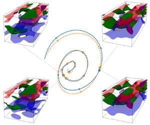
In this paper, we present applications of DMD to the data obtained from the DNS of transitional Couette and turbulent Poiseuille flows in rectangular channels. The key technical advancement here is the preprocessing of data by symmetry reduction to eliminate the degeneracies due to streamwise and spanwise translations, which resolves the well-known shortcomings (Kutz et al. Reference Kutz, Brunton, Brunton and Proctor2016; Sesterhenn & Shahirpour Reference Sesterhenn and Shahirpour2019) of DMD in systems with continuous symmetries. In such settings, the drifts in the continuous symmetry directions artificially increase the dimensionality of embeddings that can capture the dynamics reliably (Rowley & Marsden Reference Rowley and Marsden2000; Sesterhenn & Shahirpour Reference Sesterhenn and Shahirpour2019; Lu & Tartakovsky Reference Lu and Tartakovsky2020; Mendible et al. Reference Mendible, Brunton, Aravkin, Lowrie and Kutz2020; Baddoo et al. Reference Baddoo, Herrmann, McKeon, Kutz and Brunton2021). Furthermore, in spatiotemporal systems with a continuous flux, such as the Poiseuille flow considered here, the drifting motion completely dominates the DMD spectra, obscuring the physically important dynamics of the system under study. Through examples in the following, we demonstrate that the symmetry-reduced dynamic mode decomposition (SRDMD) of the channel flows resolves the aforementioned issues and reveals episodes that can be described reliably by low-dimensional linear expansions.
The paper is organized as follows. In § 2, we introduce channel flows and our computational set-up. We introduce the symmetries of channel flows and formulate our continuous symmetry reduction method in § 3. We summarize the DMD algorithm in § 4, then apply it to the symmetry-reduced DNS data from Couette and Poiseuille flows in §§ 5 and 6, respectively. We conclude with a discussion of our results and future directions in § 7.
2. Channel flows and the computational set-up
We consider flows between two parallel plates in a rectangular domain  $(x, y, z) \in [0, L_x) \times [-1, 1] \times [0, L_z)$, where $x$,
$x$,  $y$,
$y$,  $z$ are the streamwise, wall-normal and spanwise directions, respectively. We take the base-fluctuation decomposition $\boldsymbol {u}_{{total}} (\boldsymbol {x}, t) = U(y)\,\hat {\boldsymbol {x}} + \boldsymbol {u}(\boldsymbol {x}, t)$, $p_{{total}}(\boldsymbol {x}, t) = P_x (t)\,x + p (\boldsymbol {x}, t)$, where $U (y)\,\hat {\boldsymbol {x}}$ is the base (laminar) flow, and $P_x (t)$ is the spatial mean of the streamwise pressure gradient. Using these definitions, the governing Navier–Stokes equations can be written as
 \begin{equation} {\partial_t \boldsymbol{u} ={-} \boldsymbol{u}_{{total}} \boldsymbol{\cdot} \boldsymbol{\nabla} \boldsymbol{u}_{{total}} - \boldsymbol{\nabla} p + {Re}^{{-}1}\,\nabla^2 \boldsymbol{u} + \left[ {Re}^{{-}1} \partial_y^2U(y) - P_x \right] \hat{\boldsymbol{x}}, } \end{equation}
where  $\partial _a := \partial / \partial a$, and ${Re}$ is the Reynolds number. In the following, we consider two base flows, namely $U^{(C)} = y$ (Couette) and $U^{(P)} = 1 - y^2$ (Poiseuille). In both cases, the fluctuating velocity fields are periodic in the homogeneous directions, i.e. $\boldsymbol {u} (\boldsymbol {x},t) = \boldsymbol {u} (\boldsymbol {x} + L_x \hat {\boldsymbol {x}}, t) = \boldsymbol {u} (\boldsymbol {x} + L_z \hat {\boldsymbol {z}}, t)$, vanish (no-slip) at the walls, i.e. $\boldsymbol {u} (\boldsymbol {x}, t)|_{y=\pm 1} = 0$, and satisfy the incompressibility condition $\boldsymbol {\nabla } \boldsymbol {\cdot } \boldsymbol {u} = 0$. All of our results to follow are given for the fluctuations $\boldsymbol {u} = [u, v, w](x, y, z)$ from the base flows, for which we define the $L_2$ inner product and the $L_2$ norm, respectively, as
 \begin{equation} {\left\langle \boldsymbol{u}_1 , \boldsymbol{u}_2 \right\rangle := \frac{1}{2 L_x L_z} \int_0^{L_z} \int_{{-}1}^{1} \int_0^{L_x} \boldsymbol{u}_1 \boldsymbol{\cdot} \boldsymbol{u}_2 \, \mathrm{d}\kern 0.06em x\, \mathrm{d} y\, \mathrm{d}z \quad\mbox{and}\quad \|\boldsymbol{u}\| = \sqrt{\left\langle \boldsymbol{u} , \boldsymbol{u} \right\rangle}.} \end{equation}
 We utilize Channelflow 2.0 (Gibson et al. Reference Gibson2020) for the numerical integration of (2.1) in computational domains, properties of which are summarized in table 1. In all simulations, we use dynamically adjusted time steps so that the Courant–Friedrichs–Lewy number (CFL) satisfies  $0.15 \leqslant \textit {CFL} < 0.3$. Our first Couette domain W03 is identical to that of Waleffe (Reference Waleffe2003), and the second domain HKW is based on Hamilton et al. (Reference Hamilton, Kim and Waleffe1995); see table 1. For the latter, we adopt the resolution used in Viswanath (Reference Viswanath2007), which is higher than that used in Hamilton et al. (Reference Hamilton, Kim and Waleffe1995). For Poiseuille flow, we chose ${Re} = 2000$ and ${Re} = 5000$, which we refer to as P2K and P5K, respectively, in table 1 and hereafter. We determined the spatial resolutions such that the energy stored in the Fourier/Chebyshev modes with the highest wavenumbers is at least six orders of magnitude smaller than that in the lowest ones at all times. All of our domains are ‘minimal’ in the sense that if the spanwise extent is reduced, the simulations quickly laminarize. The Couette simulations are carried under the constraint $P_x = 0$, hence the fluid flux $Q_x (t) = \int _{-1}^{1} \int _0^{L_z} \boldsymbol {u} \boldsymbol {\cdot } \hat {\boldsymbol {x}}\, \mathrm {d} y\, \mathrm {d}z$ varies instantaneously. In contrast, we simulate Poiseuille flow under the constraint $Q_x = 4 L_z / 3$, which leaves $P_x (t)$ fluctuating. Additionally in the Poiseuille case, we impose symmetry invariance with respect to the midplane on the velocity fields, which restricts the dynamics into a lower-dimensional flow-invariant subspace without altering wall friction and the Reynolds stresses near the wall. For the Poiseuille systems P2K and P5K, we estimate the friction Reynolds numbers and the channel dimensions in wall units (Pope Reference Pope2000) as $({Re}_{\tau }, L_x^+, L_z^+) \approx (98, 280, 123)$ and $({Re}_{\tau }, L_x^+, L_z^+) \approx (205, 280, 120)$, respectively. Note that our spanwise domain length is slightly larger than the minimal flow unit $L_z^+\approx 100$ established in Jiménez & Moin (Reference Jiménez and Moin1991). We suspect that this is due to our symmetry constraint, which does not allow for single-wall localization of turbulent structures that was observed by Jiménez and Moin at this ${Re}$.
The laminar flows  $U(y)$, domain lengths $L_x$ and $L_z$, grid dimensions $N_x$, $N_y$, $N_z$, and additional constraints of the computational set-ups. Here, W03 and HKW correspond to the Couette domains of Waleffe (Reference Waleffe2003) and Hamilton et al. (Reference Hamilton, Kim and Waleffe1995), respectively, while P2K and P5K correspond to the Poiseuille systems at $Re=2000$ and 5000, respectively.

3. Symmetries and symmetry reduction
Both Couette and Poiseuille systems are equivariant under the translations
 \begin{equation} {\boldsymbol{T} (\delta x, \delta z) [u, v, w](x, y, z) = [u, v, w](x - \delta x, y ,z - \delta z) , } \end{equation}
where  $\delta {x} \in [0, L_x)$ and $\delta {z} \in [0, L_{z})$, and the reflection
 \begin{equation} {\boldsymbol{R}_z [u, v, w](x, y, z) = [u, v, - w](x, y, - z). } \end{equation}
Additionally, Poiseuille flow admits the equivariance under the reflection
 \begin{equation} {\boldsymbol{R}_y [u, v, w](x, y, z) = [u, - v, w](x, - y, z) } \end{equation}
with respect to the midplane; and plane-Couette flow is equivariant under the simultaneous reversal of streamwise and wall-normal directions, i.e.
 \begin{equation} {\boldsymbol{R}_{xy} [u, v, w](x, y, z) = [{-}u, -v, w]({-}x, -y, z).} \end{equation}
 For the present study, the equivariance of a flow under a symmetry group  $\mathcal {G}$ has two important consequences (Golubitsky & Schaeffer Reference Golubitsky and Schaeffer1985; Chossat & Lauterbach Reference Chossat and Lauterbach2000). (i) If $\boldsymbol {u} (\boldsymbol {x}, t)$ for $t \in [t_i, t_f]$ is a trajectory of the system, then so is $\boldsymbol {S} \boldsymbol {u} (\boldsymbol {x}, t)$, where $\boldsymbol {S} \in \mathcal {G}$. (ii) If $\boldsymbol {u} (\boldsymbol {x}, 0)$ is invariant under $\boldsymbol {S} \in \mathcal {G}$ satisfying $\boldsymbol {S} \boldsymbol {u} (\boldsymbol {x}, 0) = \boldsymbol {u} (\boldsymbol {x}, 0)$, then its forward-time evolution remains invariant under $\boldsymbol {S}$, i.e. $\boldsymbol {S} \boldsymbol {u} (\boldsymbol {x}, t) = \boldsymbol {u} (\boldsymbol {x}, t)$ for $t > 0$. We make use of (ii) when restricting our study of Poiseuille flow into the space of solutions that are invariant under (3.3). Due to the presence of continuous symmetries, (i) effectively implies that the generic solutions of Couette and Poiseuille flows have infinitely many symmetry copies due to translations and their combinations with various reflections.
Sirovich (Reference Sirovich1987b) showed that if a data set of flow states is symmetric under a continuous translation, then its proper orthogonal decomposition (POD) results in modes that align with Fourier modes in the homogeneous directions, carrying no information about the physics of the system. As a remedy, Rowley & Marsden (Reference Rowley and Marsden2000) suggested reducing the symmetry degree of freedom prior to the POD of the data obtained from a system with translation symmetry. Their method relied on an experimentally chosen template to which the simulation data are matched. As noted by the authors themselves, such a symmetry reduction method has a finite domain of applicability, the boundary of which is set by the singularity of the so-called reconstruction equation. Recently, the difficulties posed by continuous symmetries for dimensionality reduction have also received attention in the DMD and machine learning literature, and several new techniques to address them were proposed. Sesterhenn & Shahirpour (Reference Sesterhenn and Shahirpour2019) suggested a space–time rotation that can be employed at a characteristic group velocity to improve the performance of DMD in drift-dominated systems. Lu & Tartakovsky (Reference Lu and Tartakovsky2020) introduced the Lagrangian DMD, which requires one to co-evolve the solution grid along with the scalar fields. In the physics-informed DMD developed by Baddoo et al. (Reference Baddoo, Herrmann, McKeon, Kutz and Brunton2021), the DMD matrix that provides the best-fit linear system to the data is constrained to the space of matrices that commute with the symmetry operators. Finally, Kneer et al. (Reference Kneer, Sayadi, Sipp, Schmid and Rigas2022) utilize the so-called spatial translation networks to perform template matching akin to that of Rowley & Marsden (Reference Rowley and Marsden2000). Each of these methods comes with a new set of technical difficulties, and it is unclear whether they are practical for the three-dimensional complex fluid flows that we consider here. In the following, we avoid these difficulties by taking an approach similar to that of Rowley & Marsden (Reference Rowley and Marsden2000), and formulate a symmetry reduction method for preprocessing channel flow data prior to the DMD. Differently from Rowley & Marsden (Reference Rowley and Marsden2000), our method yields a symmetry reduction for all dynamics of interest.
Budanur et al. (Reference Budanur, Cvitanović, Davidchack and Siminos2015b) showed that a polar coordinate transformation in the Fourier space of a spatially extended system can be interpreted as a slice, that is, a codimension-1 manifold in the state space where each set of translation-equivalent states is represented by its unique intersection with this manifold. On applications to the Kuramoto–Sivashinsky system, Budanur et al. (Reference Budanur, Cvitanović, Davidchack and Siminos2015b) demonstrated that such a first Fourier mode slice can be used to reduce the translation symmetry of the flow for all dynamics of interest. Later, the method was adapted successfully to two-dimensional Kolmogorov flows (Farazmand Reference Farazmand2016; Hiruta & Toh Reference Hiruta and Toh2017) and three-dimensional pipe flows (Willis, Short & Cvitanović Reference Willis, Short and Cvitanović2016; Budanur et al. Reference Budanur, Short, Farazmand, Willis and Cvitanović2017; Budanur & Hof Reference Budanur and Hof2018); see Budanur, Borrero-Echeverry & Cvitanović (Reference Budanur, Borrero-Echeverry and Cvitanović2015a) for a pedagogical introduction. Here, we formulate this method for flows in rectangular channels. We begin by defining the slice templates
 $$\begin{gather} \hat{\boldsymbol{u}}'_x := \boldsymbol{f}_x (y) \cos (2 {\rm \pi}x / L_x), \end{gather}$$
 $$\begin{gather}\hat{\boldsymbol{u}}'_z := \boldsymbol{f}_z (y) \cos (2 {\rm \pi}z / L_z), \end{gather}$$
where  $\boldsymbol {f}_x (y)$ and $\boldsymbol {f}_z (y)$ are to-be-specified vector-valued functions of the wall-normal coordinate only. Let $\boldsymbol {u}$ be a solution, and let the set $\mathcal {M}_{\boldsymbol {u}}^x = \{ \boldsymbol {T} (\delta {x}, 0)\,\boldsymbol {u} \,|\, \delta x \in [0, L_x) \}$ be formed by $\boldsymbol {u}$ and its streamwise-translation copies. The key idea behind the first Fourier mode slice is the observation that any non-zero projection of $\mathcal {M}_{\boldsymbol {u}}^x$ onto the plane spanned by $\hat {\boldsymbol {u}}'_x$ and its quarter-domain shift $\boldsymbol {T}(L_x/4, 0)\,\hat {\boldsymbol {u}}'_x = \boldsymbol {f}_x (y) \sin (2 {\rm \pi}x / L_x)$ is of circular shape. Thus a transformation that fixes the polar angle $\phi _x := \arg \left (\left \langle \boldsymbol {u} , \hat {\boldsymbol {u}}'_x \right \rangle + {\rm i} \left \langle \boldsymbol {u} , \boldsymbol {T} (L_x/4, 0)\, \hat {\boldsymbol {u}}'_x \right \rangle \right )$ can be used to reduce the translation symmetry. Following analogous observations, we define $\phi _z := \arg \left (\left \langle \boldsymbol {u} , \hat {\boldsymbol {u}}'_z \right \rangle + {\rm i} \left \langle \boldsymbol {u} , \boldsymbol {T} (0, L_z/4)\,\hat {\boldsymbol {u}}'_z \right \rangle \right )$ and the symmetry-reducing transformations
 $$\begin{gather} S_x (\boldsymbol{u}) := \boldsymbol{T} \left({- \frac{\phi_x L_x}{2 {\rm \pi}}, 0}\right) \boldsymbol{u} , \end{gather}$$
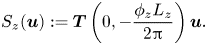 $$\begin{gather}S_z (\boldsymbol{u}) := \boldsymbol{T} \left({0, - \frac{\phi_z L_z}{2 {\rm \pi}}}\right) \boldsymbol{u} . \end{gather}$$
Noting that the slice templates  $\hat {\boldsymbol {u}}'_x (x, y)$ in (3.5) and $\hat {\boldsymbol {u}}'_z (y, z)$ in (3.6) do not depend on the $z$ and $x$ coordinates, respectively, and the translations in the $x$ and $z$ directions commute, we reduce the streamwise and spanwise translations simultaneously by simply applying (3.7) and (3.8) consecutively as
 \begin{equation} { \hat{\boldsymbol{u}} = S (\boldsymbol{u}) = S_z (S_x (\boldsymbol{u})) . } \end{equation}
 Until now, we left the wall-normal dependence of the template functions (3.5), (3.6) unspecified. In order to clarify this final point, let us first give a geometric interpretation of continuous symmetry reduction. Since symmetry reduction eliminates two continuous translation degrees of freedom, the symmetry-reduced velocity fields  ${\boldsymbol {\hat {u}}} (t)$ are confined to a submanifold in the state space with two dimensions fewer than that accommodating the original velocity fields $\boldsymbol {u} (t)$. This information, however, is not lost and can be recovered as long as one keeps track of the slice phases $\phi _x (t)$ and $\phi _z(t)$. Rowley & Marsden (Reference Rowley and Marsden2000) showed that these phases can also be obtained by integrating the reconstruction equations
 $$\begin{gather} \dot{\phi}_{x} (t) = \left({\frac{2 {\rm \pi}}{L_x}}\right) \frac{\left\langle \partial_{x} \hat{\boldsymbol{u}}'_{x} , \partial_{t} \boldsymbol{u}|_{\boldsymbol{u} =\hat{\boldsymbol{u}} (t)} \right\rangle}{ \left\langle \partial_{x} \hat{\boldsymbol{u}}'_{x} , \partial_{x} \hat{\boldsymbol{u}} (t) \right\rangle}, \end{gather}$$
 $$\begin{gather}\dot{\phi}_{z} (t) = \left({\frac{2 {\rm \pi}}{L_z}}\right) \frac{\left\langle \partial_{z} \hat{\boldsymbol{u}}'_{z} , \partial_{t} \boldsymbol{u}|_{\boldsymbol{u} = \hat{\boldsymbol{u}} (t)} \right\rangle}{ \left\langle \partial_{z} \hat{\boldsymbol{u}}'_{z} , \partial_{z} \hat{\boldsymbol{u}} (t) \right\rangle}. \end{gather}$$
Note that these phase velocities diverge if the denominators of the reconstruction equations vanish, at which point our symmetry reduction method would suffer a discontinuity. It is straightforward to confirm that these denominators are proportional to the amplitudes of the projections of the flow state  $\boldsymbol {u}$ onto the plane spanned by the respective slice template and their half-domain shift. In other words,
 $$\begin{gather} \left\langle \partial_{x} \hat{\boldsymbol{u}}'_{x} , \partial_{x} \hat{\boldsymbol{u}} (t) \right\rangle \propto \sqrt{\left\langle \boldsymbol{u} , \hat{\boldsymbol{u}}'_x \right\rangle^2 + \left\langle \boldsymbol{u} , \boldsymbol{T} (L_x/4, 0)\,\hat{\boldsymbol{u}}'_x \right\rangle^2} , \end{gather}$$
 $$\begin{gather}\left\langle \partial_{z} \hat{\boldsymbol{u}}'_{z} , \partial_{z} \hat{\boldsymbol{u}} (t) \right\rangle \propto \sqrt{\left\langle \boldsymbol{u} , \hat{\boldsymbol{u}}'_z \right\rangle^2 + \left\langle \boldsymbol{u} , \boldsymbol{T} (0, L_z/4)\,\hat{\boldsymbol{u}}'_z \right\rangle^2} , \end{gather}$$
thus as long as these projections onto the template planes do not vanish, the right-hand sides of the reconstruction equations (3.10), (3.11) remain finite. With this in mind, we determine  $\boldsymbol {f}_x (y)$ and $\boldsymbol {f}_z (y)$ as follows to maximize the projection amplitudes (3.12) and (3.13) for turbulent trajectories. Let
 $$\begin{gather} \boldsymbol{f}_x (y) = \sum_{n = 0}^{n_f} T_n(y)\,[c_x^{(x,n)} \hat{\boldsymbol{x}} + c_x^{(y,n)} \hat{\boldsymbol{y}} + c_x^{(z,n)} \hat{\boldsymbol{z}}], \end{gather}$$
 $$\begin{gather}\boldsymbol{f}_z (y) = \sum_{n = 0}^{n_f} T_n(y)\, [c_z^{(x,n)} \hat{\boldsymbol{x}} + c_z^{(y,n)} \hat{\boldsymbol{y}} + c_z^{(z,n)} \hat{\boldsymbol{z}}], \end{gather}$$
where  $T_n (y)$ are the Chebyshev polynomials of the first kind, and $c_{j}^{i,n}$ ( $i \in \{x, y, z\}$, $j \in \{x, z\}$, $n \in \{0, 1, \ldots, n_f\}$) are the coefficients that we determine by maximizing
 $$\begin{gather} \mathcal{J}_x = \sum_{k = 0}^{K} \left\langle \boldsymbol{u}(k\,\delta t) , \hat{\boldsymbol{u}}'_x \right\rangle^2 + \left\langle \boldsymbol{u}(k\,\delta t) , \boldsymbol{T} (L_x/4, 0)\,\hat{\boldsymbol{u}}'_x \right\rangle^2, \end{gather}$$
 $$\begin{gather}\mathcal{J}_z = \sum_{k = 0}^{K} \left\langle \boldsymbol{u}(k\,\delta t) , \hat{\boldsymbol{u}}'_z \right\rangle^2 + \left\langle \boldsymbol{u}(k\,\delta t) , \boldsymbol{T} (0, L_z/4)\,\hat{\boldsymbol{u}}'_z \right\rangle^2, \end{gather}$$
for a turbulent trajectory  $\{\boldsymbol {u} (t), t \in [0, K\,\delta t]\}$, under the constraints $\|\hat {\boldsymbol {u}}'_x\| = 1$ and $\|\hat {\boldsymbol {u}}'_z\| = 1$. The necessity of these unit-norm constraints can be understood by observing that (3.10) and (3.11) are invariant under the scaling of $\hat {\boldsymbol {u}}'_x$ and $\hat {\boldsymbol {u}}'_z$ by a constant. Thus if we do not apply these constraints, then the prescribed optimization would diverge by arbitrarily increasing the template amplitudes, without a reduction in phase fluctuations. In the case of Poiseuille flow, we have the additional constraint that the slice templates be $\boldsymbol {R}_y$-symmetric like the underlying flow. The cost functions (3.16) and (3.17) are the sums of squares of projection amplitudes (right-hand sides of (3.12) and (3.13)). For each domain that we study, we determine (3.14) and (3.15) truncated at $n_f = 7$ using a single turbulent trajectory sampled at steps $t_s = 0.1$. The resulting $\boldsymbol {f}_x (y)$ and $\boldsymbol {f}_z(y)$ are plotted in figure 1, and the slice templates can be downloaded from Yalnız, Marensi & Budanur (Reference Yalnız, Marensi and Budanur2022). The phase velocities (3.10), (3.11) are plotted in figure 2. As shown, although the phase speeds exhibit occasional fast episodes, they remain finite throughout our simulations. Note that in figure 2, all phase velocities but $\dot {\phi }_x$ of plane-Poiseuille flow fluctuate about zero. This is a consequence of Poiseuille flow's broken reflection symmetry in the streamwise direction due to the presence of a non-zero mean pressure gradient. Intuitively, one can understand this by considering the presence of the net drift due to the non-zero bulk velocity $U_b$ in Poiseuille flow. However, it is also important to note that $\dot {\phi }_x$ in Poiseuille flow is not equal to $2 {\rm \pi}U_b / L_x$, neither is any other phase velocity equal to $0$, the bulk velocity at their respective directions, at all times: phase velocities vary instantaneously and match the corresponding bulk velocities only when averaged over long periods.
Wall-normal dependencies of the slice templates. Columns correspond to the domains studied, with the domain name noted at the top. Each  $\boldsymbol {f}_x$ and $\boldsymbol {f}_z$ was normalized with $\max |\boldsymbol {f}_x|$ and $\max |\boldsymbol {f}_z|$, which does not affect slicing, in order for the plots to share the horizontal axes.

Finite-difference approximations  $\dot {\phi }_{x, z} (t) \approx (\phi _{x, z} (t + \eta ) - \phi _{x, z} (t))/\eta$ with $\eta = 0.1$ to the slice phase velocities (a) $\dot {\phi }_x$ and (b) $\dot {\phi }_z$, corresponding to turbulent trajectories in simulation domains considered. Here, $\dot {\phi }_{x, z}$ are normalized by $2{\rm \pi} /L_{x,z}$ to present the different domains together.

As we will explain further in § 5 through an example, the episodes with fast phase velocities in figure 2 correspond to those at which chaotic trajectories have relatively small projection amplitudes (3.12), (3.13). Observing this, one might suggest the temporal minimum of these projections as a cost function to maximize as opposed to the sums of squares (3.16), (3.17). Although we experimented with such a cost function, ultimately we opted against it because the optimization problem of maximizing a temporal minimum is non-differentiable, thus significantly more complex, since the instance of the minimum jumps during the optimization procedure. In addition to its computational simplicity, another motivation to use the cost functions (3.16) and (3.17) is that we also want the episodes with fast phase oscillations to be infrequent. Note that in all the domains that we considered, the wall-normal dependence of the spanwise slice template  $\hat {\boldsymbol {u}}_z$ has the largest contribution from the streamwise fluctuations as shown in figures 1(e–h). Remembering that all of our computational domains are minimal flow units (Jiménez & Moin Reference Jiménez and Moin1991), we interpret our optimal slice templates as those that fix the spanwise positions of streaks, since the minimal flow units are characterized by the presence of a single pair of fast/slow streaks, which appear predominantly in the first spanwise Fourier mode of streamwise velocity. Conversely, the streamwise contribution to the streamwise slice templates is much smaller (figures 1a–d) since in this direction, streaks make the largest contribution to the zeroth streamwise Fourier mode of streamwise velocity. Physically, we expect the symmetry reduction procedure to eliminate the drifts of the flow structures whose first Fourier mode components align with the slice templates. It should be noted, and can also be seen in supplementary movies 1 and 2 available at https://doi.org/10.1017/jfm.2022.1001, that drifts with respect to these structures are still present in the symmetry-reduced time evolution because in a turbulent flow, fluctuations are advected at the local mean velocity, which varies within the domain. In other words, symmetry reduction does not eliminate all drifts in the velocity fluctuations, but rather eliminates the translation degrees of freedom in the data by finding a representative state for each set of the states that can be mapped to one another via symmetry operations.
4. Symmetry-reduced dynamic mode decomposition
Let  $\xi (t)$ be the $n$-dimensional symmetry-reduced state vector corresponding to the fluid state at time $t$, let ${\varPhi ^{t}(\xi )}$ be the finite-time flow induced by the DNS and symmetry reduction, and let $\left \langle \xi _1 , \xi _2 \right \rangle$ and $\| \xi \|$ denote the $L_2$ inner product and norm, respectively, of the corresponding velocity fields as defined in (2.2a,b). Let $\xi _k$ and $\xi '_k$ be a pair of snapshots that are separated by time $\delta t$, i.e. $\xi '_{k} = {\varPhi ^{\delta t}(\xi _{k})}$. Defining the $n \times m$ ( $n \gg m$) data matrices $\varXi := [ \xi _0, \xi _1, \ldots, \xi _{m-1} ]$ and $\varXi ' := [ \xi '_0, \xi '_1, \ldots, \xi '_{m-1} ]$, we consider the linear approximation $\varXi ' \approx A \,\varXi$, where $A$ is an $n \times n$ matrix. The best fit (in the $L_2$ sense) to this approximation is given by $A = \varXi ' \varXi ^{\dagger}$, where ${\dagger}$ denotes the Moore–Penrose pseudo-inverse. We adopt the standard DMD algorithm (Tu et al. Reference Tu, Rowley, Luchtenburg, Brunton and Kutz2014; Kutz et al. Reference Kutz, Brunton, Brunton and Proctor2016), which approximates the eigenvalues and eigenvectors of $A$ without explicitly computing it, as follows. Let $\varXi \approx U \varSigma V^*$ denote the rank- $r$ (
$r$ ( $r < m$) singular value decomposition approximation of $\varXi$, where $U \in \mathbb {C}^{n \times r}$, $\varSigma \in \mathbb {C}^{r \times r}$, $V \in \mathbb {C}^{m \times r}$, and $^*$ indicates the Hermitian transpose. Noting that the columns of $U$ are the POD modes, we can rewrite the best-fit linear operator and its $r \times r$ projection onto the POD space as $A = \varXi ' V \varSigma ^{-1} U^*$ and $\tilde {A} = U^* A U = U^* \varXi ' V \varSigma ^{-1}$, respectively. Finally, we compute the eigenvalues $\varLambda _j$ and eigenvectors $\tilde {\psi }_j$ of $\tilde {A}$, from which we obtain the SRDMD modes as $\psi _j = \varXi ' V \varSigma ^{-1} \tilde {\psi }_j$. Hereafter, we refer to $\varLambda _j$ as the ‘SRDMD multipliers’ and $\lambda _j := \ln ( \varLambda _j) / \delta t$ as the ‘SRDMD exponents’. With these definitions, we can now write the SRDMD approximation of the time evolution as
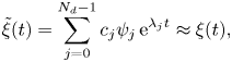 \begin{equation} {\tilde{\xi}(t) = \sum_{j = 0}^{N_d - 1} c_j \psi_j\,{\rm e}^{\lambda_j t} \approx \xi(t) ,} \end{equation}
where  $c_j$ are the SRDMD coefficients, and $N_d \leqslant r$ is the number of SRDMD modes used to reconstruct the velocity field. Following Page & Kerswell (Reference Page and Kerswell2019), we set the coefficients $c_j$ as those that minimize the cost function
 \begin{equation} {\mathcal{J}(c_0, c_1, \ldots, c_{N_d - 1}) = \sum_{k = 0}^{m - 1} \| \xi(t_k) -\tilde{\xi}(t_k) \|^2 .} \end{equation}
In the following, we refer to the SRDMD mode  $\psi _0$ with $\varLambda _j \approx 1$ ( $\lambda _j \approx 0$) as the ‘marginal mode’, and sort the rest according to their normalized spectra (Tu et al. Reference Tu, Rowley, Luchtenburg, Brunton and Kutz2014) in descending $|\varLambda _j |^{m}\,\| c_j \psi _j \|$. Note that ordering the SRDMD modes in this way amplifies (penalizes) those that grow (decay) by multiplying them with their respective multiplier raised to the power $m$.
$m$.
We compute the singular value decomposition of  $\varXi$ using the method of snapshots (Sirovich Reference Sirovich1987a) and follow Holmes, Lumley & Berkooz (Reference Holmes, Lumley and Berkooz1996) and Sirovich (Reference Sirovich1989) to truncate it such that a sufficiently large fraction $c_{\sigma }$ of the total energy is captured, and no neglected mode contains, on average, more than a small fraction $c_{\chi }$ of the energy contained in the first mode. Namely,
 \begin{equation} \sum_{i=0}^{r-1} \sigma_i^2 > c_{\sigma} \sum_{i=0}^{m-1} \sigma_i^2 \quad\mbox{and}\quad \frac{1}{m - r}\sum_{i=r}^{m - 1}\sigma_i^2 < c_{\chi} \sigma_0^2, \end{equation}
where  $\sigma _i$ are the singular values. For all of our results to follow, we set $c_{\sigma } = 0.9999$ and $c_{\chi }=0.001$, which we determined by ensuring that higher-rank truncations do not alter the leading SRDMD exponents in the first two digits.
Note that the above-summarized formulation of DMD does not necessitate the data points  $\xi _0, \xi _1, \xi _2, \ldots$ to be uniformly distributed in time. The only requirement is for the snapshot separation time $\delta t$ to be fixed across all snapshot pairs $(\xi _k, \xi '_k)$. Therefore, one can increase the number of data points corresponding to a time interval by sampling it at a time step $t_s = \delta t / n$, where $n \in \mathbb {Z}^+$. In our plane-Couette examples of § 5, we make use of this property by choosing $t_s = \delta t / 10$, whereas in our Poiseuille flow demonstrations of § 2, we use uniformly distributed samples separated by $\delta t$.
5. Relative invariant solutions and their SRDMD
Page & Kerswell (Reference Page and Kerswell2019, Reference Page and Kerswell2020) demonstrated how DMD captures dynamics of the plane-Couette flow near simple equilibria and periodic orbits defined by
 \begin{equation} {\boldsymbol{u}_{eq}(t) = \boldsymbol{u}_{eq}(0) \quad \mbox{and} \quad \boldsymbol{u}_{po}(t + T_{po}) = \boldsymbol{u}_{po}(t) , } \end{equation}
respectively. The equilibria of the plane-Couette flow belong to the flow-invariant subspaces of  $\boldsymbol {S}_1 \boldsymbol {R}_z$ and $\boldsymbol {S}_2 \boldsymbol {R}_{xy}$, where $\boldsymbol {S}_{1}$ and $\boldsymbol {S}_{2}$ are some elements of plane-Couette flow's symmetry group. Invariance of these solutions under the symmetries involving reflections $\boldsymbol {R}_z$ and $\boldsymbol {R}_{xy}$ restricts their dynamics to the space of ‘non-drifting’ velocity fields; see Gibson, Halcrow & Cvitanović (Reference Gibson, Halcrow and Cvitanović2009) for details. Besides the equilibria, these flow-invariant subspaces can also accommodate periodic orbits. Alternatively, the periodic orbits can be formed by two periods of a ‘preperiodic’ (Budanur & Cvitanović Reference Budanur and Cvitanović2016) solution defined by $\boldsymbol {u}_{ppo}(t + T) = \boldsymbol {S}_r\,\boldsymbol {u}_{ppo} (t)$, where $\boldsymbol {S}_r \in \mathcal {G}$ satisfies $\boldsymbol {S}_r^2 = I$. When such symmetries are not present, the generic solutions of plane-Couette flow exhibit streamwise and spanwise drifts. The simplest invariant solutions with drifts are the relative equilibria that satisfy
 \begin{equation} {\boldsymbol{u}_{req}(t) = \boldsymbol{T}(c_x t, c_z t)\,\boldsymbol{u}_{req}(0) ,} \end{equation}
where  $c_x$ and $c_z$ are phase velocities; and the drifting counterparts of the periodic orbits are the relative periodic orbits defined by
 \begin{equation} {\boldsymbol{u}_{rpo}(t + T_{rpo}) = \boldsymbol{T}(\Delta x_{rpo}, \Delta z_{rpo})\,\boldsymbol{u}_{rpo} (t) . } \end{equation}
 As our first demonstration of SRDMD, we apply it to trajectories in the vicinity of the relative equilibrium  $\mathrm {TW}_3$, a travelling wave originally found by Gibson et al. (Reference Gibson, Halcrow and Cvitanović2009) in the W03 domain. (The data for this solution are available in the channelflow.org database.) Figure 3(a) shows the SRDMD exponents (blue crosses) computed using five trajectories initiated as random perturbations to $\xi _{\mathrm {TW}_3}$ with perturbation amplitudes equal to $10^{-2} \|\xi _{\mathrm {TW}_3}\|$. We integrated each of these trajectories in time, and sampled the states at time steps $t_s=0.1$ in the time interval $t=[10,80]$ in which the dynamics was found to be approximately linear. To construct the data matrices $\varXi$ and $\varXi '$, we chose a separation time $\delta t=1$ between the corresponding snapshots $(\xi, \xi ')$, and we randomly selected 200 pairs of snapshots out of the $(T_w-\delta t)/t_s +1$ possible samples from each of the five trajectories, where the window length is $T_w=70$. Using the resulting SRDMD modes, we computed the best-fit coefficients $c_j^{(k)}$ as explained in § 4 for each trajectory $k = 1,2, \ldots, 5$, and ordered the exponents in descending $(1/5) \sum _{k=1}^{5}|\varLambda _j |^{m}\,\| c_j^{(k)} \psi _j \|$, i.e. according to the trajectory-averaged normalized spectrum. For comparison, figure 3(a) also shows the linear stability spectrum of $\mathrm {TW}_3$, which we approximated via Arnoldi iteration (Trefethen & Bau Reference Trefethen and Bau1997) using its channelflow implementation. As shown, the SRDMD exponents yield an approximation to the leading (ordered in descending real parts) linear stability eigenvalues of the travelling wave. Specifically, the four unstable eigenvalues with $\mathrm {Re}\, \lambda > 0$ of $\mathrm {TW}_3$ are captured very well by SRDMD, whereas the stable part of the spectrum can be only partially observed among the SRDMD eigenvalues, and a spurious complex conjugate SRDMD stable mode with $\mathrm {Re}\, \lambda < -0.05$ is also present in figure 3(a). In contrast, when we repeat this computation without symmetry reduction, we find that all non-marginal DMD modes simply lie at the drift frequency and its multiples, as seen in figure 3(d), and thus carry no information about the dynamics in the vicinity of the travelling wave.
(a) Linear stability eigenvalues ( $+$, black) of the travelling wave $\mathrm {TW}_3$ approximated via Arnoldi iteration and the SRDMD exponents ( $\times$, blue) computed from randomly perturbed trajectories in $\mathrm {TW}_3$'s vicinity. (b) A spiral-out trajectory (see main text) on $\mathrm {TW}_3$'s unstable manifold, and its SRDMD approximation visualized as a projection onto the leading SRDMD modes centred about the marginal one. (c) A spiral-in trajectory (see main text) on $\mathrm {TW}_3$'s stable manifold, and its SRDMD approximation visualized as a projection onto the leading SRDMD modes centred about the marginal one. (d–f) Same as (a–c) without symmetry reduction. Panels (a,d) have their axes normalized by $|\dot {\phi }_x^{\mathrm {TW}_3}|=0.53$, the streamwise slice velocity of $\mathrm {TW}_3$, which is constant for a travelling wave.

To further illustrate how SRDMD captures dynamics in the vicinity of a travelling wave, we perturbed  $\mathrm {TW}_3$ in the directions of the eigenvectors corresponding to the eigenvalues $\lambda _3$ and $\lambda _9$ (counting eigenvalues starting from the most unstable $\lambda _1$), and computed SRDMD approximations to these trajectories using four modes, i.e. $N_d = 4$. Each of these calculations effectively resulted in three-dimensional SRDMD approximations with the fourth mode amplitude being negligible. Indeed, after symmetry reduction, one neutral mode along with a pair of complex conjugates is sufficient for capturing spiral in/out dynamics. In figures 3(b,c), these trajectories and their SRDMD approximations are visualized as projections onto the hyperplanes spanned by the real and imaginary parts of the leading non-marginal SRDMD modes, centred around their respective marginal modes. In these and all of our state-space projections to follow, the axes correspond to $p_i = \left \langle \xi (t) - \psi _0 , \psi _i \right \rangle$ and $p_i = \left \langle \tilde {\xi } (t) - \psi _0 , \psi _i \right \rangle$ for DNS trajectories and their SRDMD approximations, respectively. As shown, SRDMD captures nicely the spiral-out/in dynamics of these unstable/stable neighbourhoods.
In order to demonstrate how the drifting motion of the travelling wave obscures the dynamics when the continuous symmetries are not taken into consideration, we repeated our spectrum calculation and approximations to the unstable/stable subspaces without reducing the continuous symmetries. As shown in figure 3(d), when the drifts are not eliminated, the DMD exponents show no resemblance to the spectrum of  $\mathrm {TW}_3$, and the individual DMD approximations are completely dominated by the drifts as indicated by the approximately circular projections in figures 3(e, f). Although DMD still approximates the trajectories shown in figures 3(e, f), essentially the only information carried in these projections is that of the drifts, and only after symmetry reduction in figures 3(b,c) can one see that these trajectories belong to different dynamical regimes.
As our second application, we adapt the DMD-based periodic orbit search method of Page & Kerswell (Reference Page and Kerswell2020) to relative periodic orbits. To this end, we simulate the plane-Couette flow in the HKW cell for a time interval  $[0, 2000]$, and sample the trajectory at steps $t_s= 0.1$. We then slide a temporal window of fixed duration $T_w = 60$ in steps $\varDelta _w=5$ along the time series, and compute the SRDMD of each window using $m=100$ randomly chosen snapshot pairs with separation time $\delta t=1$. Next, we calculate the periodicity indicator (Page & Kerswell Reference Page and Kerswell2020)
 \begin{equation} {\varepsilon (n_h) := \frac{1}{n_h \omega_f^2} \sum_{j = 1}^{n_h} |\mathrm{Im}\, \lambda_j - j \omega_f|^2, } \end{equation}
where
 \begin{equation} {\omega_f (n_h) := \frac{2}{n_h(n_h+1)} \sum_{j}^{n_h} \mathrm{Im}\, \lambda_j}, \end{equation}
and the sums are carried over the  $n_h$ SRDMD exponents with $\mathrm {Re}\, \lambda _j < \mu ^{max}$ and $0 < \mathrm {Im}\, \lambda _1 < \dots < \mathrm {Im}\, \lambda _{n_{h-1}} < \mathrm {Im}\, \lambda _{n_h}$. For an exactly periodic signal, $\varepsilon = 0$, and the DMD exponents are purely imaginary, i.e. $\mathrm {Re}\, \lambda _j = 0$ (Rowley et al. Reference Rowley, Mezić, Bagheri, Schlatter and Henningson2009). Thus $\varepsilon < \varepsilon ^{th}$ for a set of DMD exponents with real parts below a chosen threshold $\mu ^{max}$ indicates approximate periodicity (Page & Kerswell Reference Page and Kerswell2020). We set $n_h = 2$, $\mu ^{max} = 0.1$, and select guesses for relative periodic orbits from episodes with $\varepsilon < 10^{-4}$. Note that the chosen subset of SRDMD exponents contains at least one real mode, and for all the flagged episodes analysed here, we have $N_d=5$ (one real mode plus two complex conjugate pairs). We experimented with higher numbers of harmonics, i.e. $n_h=3$ and $4$ (corresponding to $N_d=7$ and $9$), but we found that increasing the number of harmonics did not provide any additional initial guess that converged to a relative periodic orbit. For the flagged episodes that we obtained, we use the state $\xi ^{(g)}$ at the time instant within the window corresponding to the minimum of the reconstruction error, the period $T^{(g)} = 2 {\rm \pi}/ \omega _f$, and the shifts $\Delta x^{(g)} = L_{x} [ \phi _{x}(t^{(g)} + T^{(g)}) - \phi _{x}(t^{(g)}) ] / (2 {\rm \pi})$ and $\Delta z^{(g)} = L_{z} [ \phi _{z}(t^{(g)} + T^{(g)}) - \phi _{z}(t^{(g)}) ] / (2 {\rm \pi})$ as initial guesses to initiate Newton–Krylov-hookstep (Viswanath Reference Viswanath2007) searches for relative periodic orbits. Here, the superscript $^{(g)}$ stands for ‘guess’. Among 16 such searches, two converged to the time-periodic solutions of the plane-Couette flow in the HKW cell. One of these orbits was a known periodic orbit of plane-Couette flow with $(T_{po}, \Delta x_{po}, \Delta z_{po}) = (64.9, 0, 0)$ and can be found in the channelflow.org database. Since our goal here is to illustrate the utility of symmetry reduction for dynamics with spatial drifts, we do not report this orbit here, and turn our attention to the other with a non-zero drift in the streamwise direction. Figures 4(a,b) show the SRDMD exponents and spectra of the DNS window that converged to a relative periodic orbit $\mathrm {RPO}_{79.4}$ with $(T_{rpo}, \Delta x_{rpo}, \Delta z_{rpo}) = (79.4, 0.356 L_x, 0)$. Note that the converged orbit's period is approximately $4/3$ s of the DMD time window, demonstrating that SRDMD is capable of producing an initial condition for a relative periodic orbit search even when the orbit is not followed by the chaotic dynamics for a full period. This can also be seen by comparing the state-space projections of the guess episode shown in figure 4(c) to that of the converged orbit in figure 4( f) onto the subspaces spanned by the leading non-marginal SRDMD modes. Hence SRDMD successfully extends the periodic orbit detection method of Page & Kerswell (Reference Page and Kerswell2020) to the relative periodic orbits with spatial drifts. The SRDMD of the converged orbit computed using snapshots separated by $\delta t = 1$ along one full period approximates a Fourier expansion, as indicated by the fact that the near-neutral (with $\mathrm {Re}\, \lambda < 10^{-4}$) exponents are located at the harmonics of $f = 1 / T_{rpo}$, as shown in figure 4(e). This is expected since continuous symmetry reduction transforms the relative periodic orbit to a periodic one, for which the DMD corresponds to a Fourier expansion (Rowley et al. Reference Rowley, Mezić, Bagheri, Schlatter and Henningson2009). For comparison, in figures 4(g,h), we show the DMD exponents corresponding to the same data set and spectra of the relative periodic orbit without reducing its symmetry, which shows no resemblance to that of a Fourier series. Finally, figure 4(i) shows the state-space projection of the converged relative periodic orbit without symmetry reduction, where the separation of the initial and final states is seen clearly. Although figure 4(i) suggests that DMD without the symmetry reduction still yields a decent approximation to the periodic orbit, the corresponding DMD spectrum has a leading non-marginal DMD eigenvalue that is negative real, i.e. non-oscillatory, as shown by the orange marker in figures 4(g,h). The difference between the initial and final states of the orbit is also visible in supplementary movie 3, where the flow structures of the initial and final states appear at the same spots only after symmetry reduction.
(a) SRDMD exponents and (b) spectrum of the episode from which the initial guess for a relative periodic orbit  $\mathrm {RPO}_{79.4}$ is constructed. (c) State-space projection of this episode and its SRDMD approximation onto the plane spanned by the leading non-marginal SRDMD modes centred around the marginal mode. (d) SRDMD exponents and (e) spectrum of $\mathrm {RPO}_{79.4}$. ( f) State-space projection of $\mathrm {RPO}_{79.4}$ and its SRDMD approximation. (g) DMD exponents and (h) DMD spectrum of the same orbit without symmetry reduction; and (i) the corresponding state-space projections. In (b,e) and (h), $f_j = |\mathrm {Im}\, \lambda _j| / 2{\rm \pi}$ and the dashed vertical lines correspond to multiples of the fundamental frequency $2{\rm \pi} / T_{rpo}$, where $T_{rpo}$ is the period of $\mathrm {RPO}_{79.4}$.

Figure 5(a) shows the streamwise slice phase velocity  $\dot {\phi }_x$ along one period of $\mathrm {RPO}_{79.4}$ approximated by finite differences $\dot {\phi }_x \approx (\phi _x (t + \eta ) - \phi _x (t))/\eta$ and the reconstruction equation (3.10), for which we approximated the state-space velocity as $\partial _t \boldsymbol {u} \approx (\boldsymbol {u} (t + \eta ) - \boldsymbol {u} (t)) / \eta$ and used $\eta =0.01$ for both finite difference approximations. As shown, near the midpoint of the shown time window, the phase velocity momentarily approaches $\dot {\phi } \approx -10$, the effect of which can also be seen as a fast drift in supplementary movie 3. Figure 5(b) shows that this instance coincides with a near-zero of the denominator of the reconstruction equation (3.10), which accentuates the instantaneous decrease of the numerator term, as shown in figure 5(c). This illustrates an important property of our symmetry reduction method: even though instantaneous fast oscillations can be introduced as an artefact, the net drift of an invariant solution, in this case a relative periodic orbit, is zero for the totality of the orbit, i.e. one full period.


6. Locally linear approximations by SRDMD
Through the examples of the previous section, we demonstrated how symmetry reduction enables DMD to capture the transitional/low- $Re$ dynamics in the vicinity of the relative invariant solutions of plane-Couette flow with spatial drifts. We now turn our attention to plane-Poiseuille flow domains P2K and P5K, corresponding to ${Re} = 2000$ and $5000$, respectively; see table 1. Both of these domains are significantly more complex than the settings considered in the previous section, hence searching for invariant solutions in them is impractical. As we will illustrate, one can nevertheless utilize SRDMD in this problem to discover turbulent episodes that can be approximated transiently by a low-dimensional linear expansion.
We consider turbulent channel flow simulations in P2K and P5K, each spanning a time interval  $[0, 2000]$. We compute SRDMD of the data sets $\varXi = \left [ \xi _0, \xi _1, \ldots, \xi _{m-1} \right ]$ and $\varXi ' = \left [ \xi _1, \xi _2, \ldots, \xi _{m} \right ]$, where $\xi _n$ are the symmetry-reduced fluid states sampled at $\delta t$ over sliding time windows of length $T_w$. In P2K, we took $\delta t = 1$ and $T_w \in \{30, 60, 100\}$, whereas in P5K, we set these to half of their values, i.e. $\delta t = 0.5$ and $T_w \in \{15, 30, 50\}$, approximately matching the P2K values in wall units. In order to compare different episodes and window lengths, we construct SRDMD approximations (4.1) with $N_d = 11$ (or 12, depending on the number of complex conjugate exponents in the dominant part of the SRDMD spectrum, such that if a complex mode is in the spectrum, so is its complex conjugate). We evaluate the accuracy of SRDMD by measuring the residual
 \begin{equation} {\bar{\mathcal{R}} (t) = \frac{1}{m} \sum_{k = 0}^{m - 1} \frac{\| \tilde{\xi}(t + k\,\delta t) -\xi(t + k\,\delta t) \|}{ \| \xi(t + k\,\delta t) \| },} \end{equation}
which is the mean relative error of the SRDMD approximation (4.1) to the symmetry-reduced DNS states in the same time window  $[t, t+T_w)$. Figure 6 shows the residuals (6.1) of our SRDMD approximations with $N_d \leqslant 12$ to the sliding windows of the turbulent channel flow data. Low-error episodes are detected along the turbulent trajectory and appear to be clustered around certain time instants, for example around $t \approx 250$, 950 and 1250 in figure 6(a), thus signalling portions of the turbulent evolution that can be well captured by a reduced linear expansion. As expected, a linear approximation is more successful for shorter times, and accordingly the dips in the $\bar {\mathcal {R}}(t)$ curves are most marked for the shortest window lengths $T_w=30$ (P2K) and $T_w = 15$ (P5K), although they are still distinguishable for longer time windows. In the following, we decided to focus on $T_w = 60$ and $T_w = 30$ in P2K and P5K, respectively (orange curves in figure 6), which are the longest time windows of those analysed above where clear low-error episodes ( $\bar {\mathcal {R}} < 0.1$) were detected. In the rest of this section, different dynamical behaviours captured by the SRDMD approximations at these time window lengths will be illustrated.
SRDMD residuals (6.1) in (a) the P2K domain for time windows of duration  $T_w=30$, 60, 100, and (b) the P5K domain for $T_w=15$, 30, 50. Time windows were slid across the time series in steps $\varDelta _w=5$. Dashed vertical lines correspond to the initial times of the windows that are presented in figures 7–10.

Figure 7(a) shows the SRDMD spectrum of the data window corresponding to  $t \in [1280, 1340)$ in P2K, where the coloured crosses indicate the dominant part of the spectrum, and the black ones show the first three discarded modes. To illustrate the flow structures captured by SRDMD, figures 7(b–d) show three-dimensional visualizations of $\psi _0$, $\mathrm {Re}\, \psi _1$ and $\mathrm {Im}\, \psi _1$, respectively. In figures 7(b–d) and the rest of the flow visualizations of this paper, the red and blue isosurfaces show $u = 0.5\, \max u$ and $u = 0.5\, \min u$, respectively, and the green and purple isosurfaces show $\omega _x = 0.5\, \max \omega_x$ and $\omega_x = 0.5\, \min \omega _x$, respectively, where $\omega _x$ is the streamwise vorticity. Once again, for comparison in figure 7(e) we show the DMD spectrum, without symmetry reduction, of the same episode. For this computation, we needed a temporal resolution $\delta t = 0.1$ because the time scale associated with advection is much faster than those of the coherent structures. As visualized in figures 7(b–d), the SRDMD modes represent the full complexity of the turbulent episode that they approximate, and remarkably, their linear time evolutions exhibit generation and disappearance of coherent structures as shown in supplementary movie 4. As shown in figure 7(e), in the absence of symmetry reduction, the dominant frequency of the spectrum appears near the drift frequency $f_{d} = U_b/L_x \approx 0.23$, where $U_b=2/3$ is the bulk velocity marked by a dashed line in figure 7(e). In contrast to the complex flow structures captured by the SRDMD, in this case the marginal mode (figure 7f) shows elongated structures, and the leading non-marginal DMD mode aligns with the first streamwise Fourier mode (figures 7g,h), as signified by the fact that $\mathrm {Im}\, \psi _1$ (figure 7g) is virtually the same as $\mathrm {Re}\, \psi _1$ (figure 7h) up to a quarter-domain shift in the $x$ direction. We see that even for the limited time window that we consider here, the streamwise drift of channel flow completely dominates its DMD.
SRDMD in the time window  $t \in [1280,1340)$ of the P2K domain. (a) Normalized SRDMD spectrum where $f_j = |\mathrm {Im}\, \lambda _j| / 2{\rm \pi}$. The coloured symbols correspond to the modes that are included in the sum (4.1), while the black symbols are the first three discarded modes. (b–d) Three-dimensional visualizations of the SRDMD modes (b) $\psi _0$, (c) $\mathrm {Re}\, \psi _1$ and (d) $\mathrm {Im}\, \psi _1$, where the red (blue) isosurfaces show $u = 0.5 \max u\ (u = 0.5 \min u)$ and the green (purple) indicate the streamwise vorticity isosurfaces $\omega _x = 0.5 \max \omega_x\ (\omega_x = 0.5 \min \omega _x)$. (e) DMD spectrum (without symmetry reduction) of the same episode. The dashed vertical line corresponds to the drift frequency $f_{d} = U_b/L_x$, where $U_b$ is the bulk velocity. ( f–h) Three-dimensional visualizations of the DMD modes. The colours of the bounding boxes in the three-dimensional visualizations correspond to the (SR)DMD modes marked with the same colours in the spectra in (a) and (e).

As illustrations of different dynamical regimes captured by SRDMD, in figure 8, we show state-space projections of several time windows and their SRDMD approximations onto the subspaces spanned by complex conjugate SRDMD modes. In figures 8(a,b), we see spiral-out/in dynamics corresponding to the low-error episodes in figure 6(a), reminiscent of similar episodes that we illustrated for a travelling wave in figures 3(c,d). In figure 8(c), we show a nearly periodic trajectory at  ${Re} = 2000$, which we detected at a minimum of the periodicity indicator (5.4) with $n_h=4$, $\mu ^{max} = 0.1$ and $\varepsilon ^{th} = 2 \times 10^{-3}$. As expected, at ${Re} = 5000$ the dynamics is significantly more complex, nevertheless the resemblance of state-space projections of DNS data and their SRDMD approximations can also be seen in figures 8(a–c). Differently from figures 8(a,b), here we do not see simple spiral-in/out dynamics, but several instabilities at play, as illustrated by figures 8(d,e), which show the projections of the same low-error episode into the subspaces spanned by the corresponding SRDMD modes $\psi _2$ and $\psi _4$. Finally, figure 8( f) shows a nearly periodic episode in the P5K domain detected at a minimum of the periodicity indicator (5.4) using the same parameters as P2K.
State-space projections of DNS trajectories and their SRDMD approximations from (a–c) the P2K domains and (d–f) the P5K domains, onto complex SRDMD modes centred around the marginal modes. The episodes correspond to (a)  $t \in [240, 300)$, (b) $t \in [1280, 1340)$, (c) $t\in [1300,1360)$ in P2K, and (d,e) $t \in [425, 455)$ and ( f) $t\in [1680,1710)$ in P5K.

For the spiral-out event starting at  $t=1280$ in P2K (figure 8b), we compare the evolution of the flow structures reconstructed using SRDMD to those of the original turbulent dynamics; see figure 9 and supplementary movie 4. The SRDMD spectrum and the first two SRDMD modes for this time window were displayed in figure 7. As shown in figure 9, SRDMD can capture the evolution of streaks and rolls, visualized as isosurfaces of streamwise velocity and streamwise vorticity, respectively, with only 12 modes. In particular, it can capture the initial growth of the rolls, which then break up into smaller structures and appear to decay towards the end of the time window, while the streaks start meandering.
Three-dimensional visualizations of symmetry-reduced flow states and their SRDMD approximations for the time window  $t \in [1280, 1340)$ in the P2K domain.

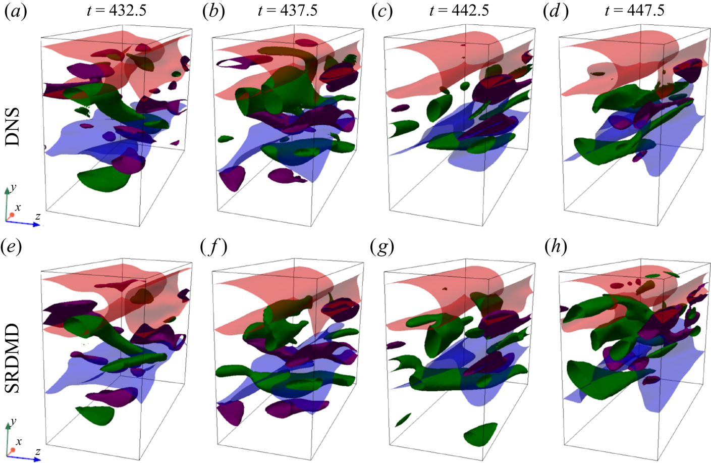
As our final illustration, in figure 10, we show flow states and their SRDMD approximations corresponding to the time window  $[425, 455)$ of the P5K domain. Although the one-to-one correspondence of vortical structures is not as evident as in the P2K configuration, the streak evolution is still captured by the SRDMD approximation.
Three-dimensional visualizations of symmetry-reduced flow states and their SRDMD approximations for the time window  $t \in [425, 455)$ in the P5K domain.
7. Conclusion and outlook
In this paper, we developed a continuous symmetry reduction method for three- dimensional flows in rectangular channels and applied it to plane-Couette and plane-Poiseuille simulations at various  ${Re}$ to illustrate the necessity of symmetry reduction for preprocessing the data prior to DMD. We showed in § 5 that the combination of symmetry reduction and DMD, which we named SRDMD, yields linear modal expansions that capture the stable/unstable dynamics in the vicinity of a travelling wave, whereas the standard DMD of the same data was dominated by the drifts. Moreover, utilizing SRDMD, we extended the Page & Kerswell (Reference Page and Kerswell2020) DMD-based periodic orbit search method to relative periodic orbits and showed that a guess for a relative periodic orbit can be generated by SRDMD even when turbulence does not follow the relative periodic orbit for a full period, enabling relative periodic orbit searches that would not have been possible via recurrent flow analysis (Chandler & Kerswell Reference Chandler and Kerswell2013). In the light of recent evidence (Krygier, Pughe-Sanford & Grigoriev Reference Krygier, Pughe-Sanford and Grigoriev2021; Yalnız, Hof & Budanur Reference Yalnız, Hof and Budanur2021; Crowley et al. Reference Crowley, Pughe-Sanford, Toler, Krygier, Grigoriev and Schatz2022) that the approaches of turbulence to periodic solutions are often not for a full period, we think that SRDMD-based approaches can accelerate relative periodic orbit searches in future studies.
One of the main motivations behind studying the invariant solutions of the Navier–Stokes equations follows from the observation that, together with their stable and unstable manifolds, the invariant solutions provide ‘efficient’ bases for approximating chaotic dynamics in their vicinity. This is also illustrated in figure 4 of the present paper, where the state-space projection of the turbulent trajectory in figure 4(c) shows the features of the nearby relative periodic orbit, shown in figure 4( f). The main message that we hope to convey with the present paper is that such seemingly simple dynamics can also be found in more complicated settings, such as the turbulent plane-Poiseuille flow that we studied here. We would like to point out the similarities between the Poiseuille flow state-space projections shown in figures 8(a,b) and those in the vicinity of a simple travelling wave shown in figures 3(b,c). Although the spatial structures captured by the SRDMD modes are considerably complex, as illustrated in figures 7(b,c) and 9 in the Poiseuille case, the temporal dynamics is surprisingly similar to that in the vicinity of a travelling wave. Similarly, the state-space projection of the nearly periodic Poiseuille flow episode in figure 8(c) is reminiscent of that of an actual shadowing of a relative periodic orbit by turbulence shown in figure 4(c). In the light of these observations, we speculate that a modelling paradigm wherein one searches for simple data-driven models that apply to specific state-space regions could be a viable strategy for extending dynamical systems approaches to turbulence to regimes that are more complicated than those in which invariant solutions can be found.
While symmetry reduction enables us to apply DMD to flows with continuous symmetries, it of course does not eliminate limitations that are intrinsic to DMD itself. One of these is already apparent in figure 6, where the episodes with low reconstruction error mostly disappear when the SRDMD window is extended to  $T_w = 100$ and $T_w = 50$ in the P2K and P5K domains, respectively. In general, we do not expect to find low-dimensional SRDMD approximations for longer time horizons since even though DMD modes are non-orthogonal and can represent nonlinear processes such as generation of vortices, the temporal dynamics constructed by them is still linear. Recently, Linot & Graham (Reference Linot and Graham2020) have shown that a combination of symmetry reduction, an autoencoder and a reservoir computer can be used to approximate the spatiotemporally chaotic dynamics of the one-dimensional Kuramoto–Sivashinsky equation. Replacing DMD with such deep learning methods can extend the prediction horizon beyond what can be approximated by SRDMD. Similar to the finite time horizon, we also expect SRDMD to perform poorly in larger domains since turbulent flows have finite correlation lengths. This can be seen readily by comparing the snapshots in figure 9 to those in figure 10, where the height difference of the two domains, which have the same length and width in wall units, is apparent. Consequently, more flow structures are present in the wall-normal extent of the ${Re}=5000$ domain, and the corresponding SRDMD approximations in figures 8(b,e) are considerably more complex. One obvious remedy to this might be replacing the $L_2$ inner product (2.2a,b) that we used here with one incorporating a spatial filter that isolates a shorter wall-normal extent, or any other dynamical region of interest if SRDMD is applied to a flow in a larger domain.
Finally, we would like to note that in addition to it being the first continuous symmetry reduction method for channel flows, a novel aspect of the present formulation is our optimization-based determination of the wall-normal dependence of the slice templates. Previous implementations (Willis et al. Reference Willis, Short and Cvitanović2016; Budanur & Hof Reference Budanur and Hof2017, Reference Budanur and Hof2018) of the first Fourier mode slice in three-dimensional pipe flows in which both homogeneous (axial and azimuthal) and inhomogeneous (radial) directions are present relied on trial-and-error in determining the radial dependence of slice templates. The template optimization procedure developed here provides a systematic alternative to this, which we recommend for future applications of the first Fourier mode slice in similar set-ups. In hopes to lower the technical barriers for such future applications, we provide our codes in Yalnız et al. (Reference Yalnız, Marensi and Budanur2022) as examples.
Supplementary movies
Supplementary movies are available at https://doi.org/10.1017/jfm.2022.1001.
Funding
E.M. acknowledges funding from the ISTplus fellowship programme. G.Y. and B.H. acknowledge a grant from the Simons Foundation (662960, BH).
Declaration of interests
The authors report no conflict of interest.


 Open access

