1. Introduction
The study of the fluid flow saturated with porous substances started with the pioneering work by Darcy (Reference Darcy1856) in the middle of the nineteenth century. One of the attractive features of Darcy’s model is its similarity to Ohm’s law in electricity and Fourier’s law in heat conduction, which makes it mathematically simple and convenient to use. However, such simplified linear relations are not always sufficient for accurately describing flow behaviour in porous media, particularly under complex flow conditions. Consequently, further modifications and extensions are often required to capture the actual transport characteristics more realistically.
Forchheimer (Reference Forchheimer1901) introduced a nonlinear correction to include inertial effects at moderate and larger Reynolds numbers. This improvement of the Darcy model added a new quadratic drag term, which makes the relation more appropriate for flows with deviations from pure viscous behaviour. The coefficients associated with the nonlinear resistance are generally determined empirically using correlations such as the Ergun relation proposed by Ergun (Reference Ergun1952). These correlations provide a practical way for estimating the additional flow resistance encountered in real porous media.
A further advancement was introduced in the seminal work of Brinkman (Reference Brinkman1947), who attempted to bridge the gap between clear fluid flow and Darcy flow by incorporating an effective viscosity term into the momentum equation. This extension enables the model to capture viscous shear effects, boundary-layer behaviour and confinement effects near solid boundaries. Despite these advantages, the Brinkman model alone does not account for nonlinear inertial drag effects that become significant at moderate and high flow velocities, nor does it explicitly incorporate variations in porous structure and porosity. To overcome these limitations, subsequent studies combined the contributions of Darcy, Brinkman and Forchheimer into the generalised Darcy–Brinkman–Forchheimer (DBF) model (Lauriat & Prasad Reference Lauriat and Prasad1989; David, Lauriat & Cheng Reference David, Lauriat and Cheng1991; Karmakar, Reza & Sekhar Reference Karmakar, Reza and Sekhar2019). The DBF model provides a more comprehensive representation of porous medium flow over a wide range of permeability and Reynolds number regimes by simultaneously accounting for viscous diffusion, linear porous resistance and nonlinear inertial drag effects, making it highly relevant for modern engineering and transport applications.
Flow and heat transfer in isotropic porous media have grown significantly due to its applications in real-life technologies such as packed-bed reactor, heat exchanger and thermal insulation systems. The impact of inertia, spatially varying porosity and Brinkman friction on temperature and velocity distributions were examined by Poulikakos & Renken (Reference Poulikakos and Renken1987). Another study conducted by Huang & Vafai (Reference Huang and Vafai1994) demonstrated how a porous block incorporation may increase cooling efficiency. Hadim (Reference Hadim1994) further demonstrated that heat transfer behaviour in porous structures is highly sensitive to local heating conditions and the imposed boundary conditions. Nield, Junqueira & Lage (Reference Nield, Junqueira and Lage1996) conducted a theoretical examination of porous filled channels under uniform heat-flux and isothermal plate conditions. Numerical investigations by Sung, Kim & Hyun (Reference Sung, Kim and Hyun1995) demonstrated that the location of porous regions strongly influences the resulting convection patterns and flow development. Torabi et al. (Reference Torabi, Peterson, Torabi and Karimi2016) and Habib et al. (Reference Habib, Karimi, Yadollahi and Borhani2020) examined pore-scale transport behaviour and dynamic thermal responses in porous media systems. Research by Hooman & Gurgenci (Reference Hooman and Gurgenci2007) showed that strong hydrodynamic and thermal development occurs in the entrance region of porous channels. The developing region was found to significantly influence the overall flow and heat transfer behaviour. In a related study, Hooman, Hooman & Mohebpour (Reference Hooman, Hooman and Mohebpour2008) demonstrated that these developing regions contribute considerably to entropy generation and mechanical losses within porous systems. Some more related studies can be found from Satyamurty & Bhargavi (Reference Satyamurty and Bhargavi2010) and Yadav & Roshan (Reference Yadav and Roshan2024).
In comparison, studies on anisotropic porous media have expanded more recently, driven by practical interest in materials whose permeability varies with direction. Early work by Wang, Thauvin & Mohanty (Reference Wang, Thauvin and Mohanty1999) drew attention to non-Darcy behaviour in flow through anisotropic porous medium. Subsequent investigations by Degan et al. (Reference Degan, Vasseur and Bilgen1995, Reference Degan, Zohoun and Vasseur2002, Reference Degan, Akowanou and Awanou2007) explored forced and natural convection in anisotropic layers, revealing how directional permeability affects flow and temperature distributions. Flow reversal in wavy anisotropic channels was reported by Karmakar & Raja Sekhar (Reference Karmakar and Raja Sekhar2017) and Pramanik & Karmakar (Reference Pramanik and Karmakar2026), while Karmakar et al. (Reference Karmakar, Reza and Sekhar2019) further demonstrated how varying permeability ratios influence heat transfer rates and velocity fields subjected to isoflux boundaries. Buonomo et al. (Reference Buonomo, di Pasqua, Manca, Nappo and Tamburrino2022) examined entropy production in nanofluid-based forced convection, showing enhanced thermal performance in both isotropic and anisotropic configurations. Recent investigations by Jaiswal et al. (Reference Jaiswal, Yadav, Yadav and Sharma2025) analysed entropy generation in unsteady micropolar fluid flow through anisotropic porous media, highlighting the effects of anisotropic resistance on thermodynamic irreversibility. The physics of generalised Couette flow involving immiscible fluids in anisotropic porous structures was further explored by Jaiswal & Yadav (Reference Jaiswal and Yadav2024), while Yadav et al. (Reference Yadav, Jaiswal, Verma and Chamkha2023) investigated magnetohydrodynamic transport of immiscible Newtonian fluids in porous regions with variable permeability functions. Collectively, these contributions underscore the important role that anisotropy plays in defining the thermal and hydrodynamic behaviour of porous-filled channels.
The existence and uniqueness of solutions of fluid flow equations for incompressible Newtonian and non-Newtonian fluids have been crucial in the mathematical study of fluid dynamics. The global existence of weak solutions for the three-dimensional Navier–Stokes equations was established by Leray (Reference Leray1934). Under compactly supported forcing, Guillod, Korobkov & Ren (Reference Guillod, Korobkov and Ren2023) established the existence and uniqueness of stationary flow solution in the whole plane. Caffarelli, Kohn & Nirenberg (Reference Caffarelli, Kohn and Nirenberg1982) established the partial regularity theory for suitable weak solutions of the Navier–Stokes equations and showed that the singular set has zero one-dimensional Hausdorff measure. Skrzypacz & Wei (Reference Skrzypacz and Wei2017) investigated the solvability of the DBF equations for the isotropic case.
Although extensive research has been carried out on porous medium flows, most available analytical solutions are restricted to the classical Darcy model or simplified extensions of it. Analytical studies for more complex porous flow problems are still limited. To overcome these limitations, computational fluid dynamics (CFD) techniques such as finite difference methods (FDM), finite volume methods (FVM), finite element methods (FEM) and spectral methods have been widely employed for solving the nonlinear partial differential equations (PDEs) governing porous medium transport. However, there are some limitations on these traditional methods. For instance, creating computational meshes can often be time-consuming, subjective and tedious. In recent years, neural network-based solutions have come as an interesting alternative to solve PDEs (Lagaris, Likas & Fotiadis Reference Lagaris, Likas and Fotiadis1998). These models are both fast and flexible in complex situations. Physics-informed neural networks (PINNs), first proposed by Raissi, Perdikaris & Karniadakis (Reference Raissi, Perdikaris and Karniadakis2019), have attracted much interest among them. PINNs use automatic differentiation to represent differential operators without need to mesh or discretise (Paszke et al. Reference Paszke, Gross, Chintala, Chanan, Yang, DeVito, Lin, Desmaison, Antiga and Lerer2017). This approach overcomes many of the drawbacks of the conventional CFD methods. Performance, stability and application of PINNs to complex physical problems have been the subject of recent developments. Mattey & Ghosh (Reference Mattey and Ghosh2022) introduced backward compatible PINNs (bcPINNs), which train individual neural networks over partitioned time domains without the computational burden of end-to-end temporal training. Similarly, Wang, Sankaran & Perdikaris (Reference Wang, Sankaran and Perdikaris2022) proposed Causal PINNs, where a causality-weighted loss function dynamically updates the contribution of different residual terms, thereby improving convergence for stiff nonlinear systems. Several advanced variants of PINNs have also been developed to improve performance for complex physical systems. Bayesian PINNs (B-PINNs) by Yang, Meng & Karniadakis (Reference Yang, Meng and Karniadakis2021) incorporate uncertainty quantification, making them effective for handling noisy data and reducing overfitting. Chiu et al. (Reference Chiu, Wong, Ooi, Dao and Ong2022) developed coupled-automatic-numerical PINNs (CAN-PINNs), which combine automatic and numerical differentiation techniques to improve accuracy, particularly for complex geometries. Domain decomposition approaches have also gained significant attention in recent years. Recent neural network-based computational studies related to fluid dynamics and transport phenomena can be found from Biswas & Anand (Reference Biswas and Anand2023), Singh & Yadav (Reference Singh and Yadav2026).
Despite growing interest in porous medium flows, several key research gaps remain unaddressed. First, there is a lack of rigorous mathematical treatment for anisotropic DBF flows, most existing studies focus on isotropic medium, and do not establish existence and uniqueness results under variational (weak) formulations for anisotropic cases. Second, the influence of spatially varying tensorial permeability in anisotropic porous medium in the developing region of a channel has not been thoroughly investigated in terms of its impact on flow behaviour and mathematical modelling. Third, the application of PINNs to porous media flows with anisotropic permeability remains limited, particularly in approaches that aim to integrate theoretical rigour with computational efficiency.
To address the identified research gaps, this work investigates the DBF equations for incompressible flow in anisotropic porous channels through a variational (weak) formulation. The study combines mathematical analysis with a PINN framework, enabling a mesh-free, unsupervised approach for solving the governing equations and predicting the flow field. The main objectives of the study are:
-
(i) to derive a weak form of the nonlinear DBF equations, and establish the existence and uniqueness of solution for the weak form;
-
(ii) to analyse directional flow behaviour in the developing region of the porous channel;
-
(iii) to implement a PINN-based framework by relying entirely on the governing equations and boundary conditions.
The organisation of this manuscript is as follows. Section 2 presents the formulation of the physical problem. Section 3 applies the Browder–Minty theorem to establish the existence and uniqueness of the solution. Section 4 provides a brief overview of the neural computational approach. Section 5 compares the neural network results with analytical solutions and existing literature. Section 6 presents the graphical results and analyses them. Finally, § 7 summarises the study and presents the main conclusions.
2. Mathematical formulation
This study considers a two-dimensional, steady, incompressible and laminar flow of a Newtonian fluid through a rectangular channel filled with an anisotropic porous medium saturated with fluid. The flow is assumed to be fully saturated, and the thermophysical properties of the fluid and porous medium, including density and viscosity, are taken to be constant throughout the medium. The porous medium exhibits directional permeability, represented through an anisotropic permeability tensor. The flow resistance within the porous structure is modelled using the generalised DBF equation, which accounts for viscous diffusion, Darcy drag and inertial resistance effects. The channel walls are located at $y=-L$
and
$y=-L$
and $y=L$
, as shown in figure 1. A uniform inlet velocity
$y=L$
, as shown in figure 1. A uniform inlet velocity $u_0$
is prescribed at the channel entrance, while no-slip conditions are imposed along the channel walls.
$u_0$
is prescribed at the channel entrance, while no-slip conditions are imposed along the channel walls.
Diagrammatic view of the physical situation.

Let $K_1$
and
$K_1$
and $K_2$
be the permeabilities along the two principal directions of the porous medium. Also, let
$K_2$
be the permeabilities along the two principal directions of the porous medium. Also, let $\alpha$
denote the angle of inclination between the
$\alpha$
denote the angle of inclination between the $x$
-axis and the principal permeability direction corresponding to
$x$
-axis and the principal permeability direction corresponding to $K_2$
. The overall permeability of the anisotropic porous medium is therefore represented by the second-order permeability tensor (Degan, Zohoun & Vasseur Reference Degan, Zohoun and Vasseur2002),
$K_2$
. The overall permeability of the anisotropic porous medium is therefore represented by the second-order permeability tensor (Degan, Zohoun & Vasseur Reference Degan, Zohoun and Vasseur2002),
 \begin{equation} \boldsymbol{\textit {K}}= \left [ {\begin{array}{cc} K_1 \sin ^2 \alpha +K_2 \cos ^2 \alpha & (K_2 - K_1)\sin \alpha \cos \alpha \\[3pt] (K_2 - K_1)\sin \alpha \cos \alpha & K_2 \sin ^2 \alpha +K_1 \cos ^2 \alpha \\ \end{array} } \right ]\!. \end{equation}
The permeability tensor characterises the directional resistance offered by the porous medium to fluid motion. Unlike isotropic porous media, where the resistance is identical in all directions, anisotropic permeability allows the flow resistance to vary with orientation. The off-diagonal components of the tensor represent coupling between the axial and transverse momentum transport due to the inclined permeability directions. Consequently, variations in the permeability ratio and inclination angle significantly influence the velocity distribution, pressure gradient and hydrodynamic development within the channel. Such anisotropic behaviour is commonly encountered in layered geological formations, fibrous materials, biological tissues and engineered porous structures.
2.1. Governing equations and boundary conditions
Under the given assumptions, the continuity and momentum equations for this problem are as follows (Nield & Bejan Reference Nield and Bejan2006):
 \begin{equation} \boldsymbol{\nabla } \cdot \boldsymbol{\textit {v}}=0 , \end{equation}
 \begin{equation} 0=-\boldsymbol{\nabla }p+\frac {\mu _{e}}{\epsilon }{\nabla} ^2 \boldsymbol{\textit {v}}-\mu \boldsymbol{\textit {K}}^{-1}\boldsymbol{\textit {v}}-\frac {1.75\rho }{\sqrt {150}\epsilon ^{3/2}} \boldsymbol{\textit {K}}^{-1/2} \boldsymbol{\textit {v}}|\boldsymbol{\textit {v}}|. \end{equation}
In (2.2)–(2.3), $\boldsymbol{\textit {v}}$
is the velocity vector,
$\boldsymbol{\textit {v}}$
is the velocity vector, $\rho$
is the density,
$\rho$
is the density, $p$
is the pressure and
$p$
is the pressure and $\mu$
is the viscosity of the fluid. Additionally,
$\mu$
is the viscosity of the fluid. Additionally, $\mu _{e}$
is the effective viscosity of the medium and
$\mu _{e}$
is the effective viscosity of the medium and $\epsilon$
is the porosity of the medium.
$\epsilon$
is the porosity of the medium.
In the current study, the convective acceleration term $\boldsymbol{\textit {v}}\boldsymbol{\cdot }\boldsymbol{\nabla }\boldsymbol{\textit {v}}$
is neglected because the porous medium is assumed to possess very low permeabilities (
$\boldsymbol{\textit {v}}\boldsymbol{\cdot }\boldsymbol{\nabla }\boldsymbol{\textit {v}}$
is neglected because the porous medium is assumed to possess very low permeabilities ( $K_1$
and
$K_1$
and $K_2$
). Under such conditions, the flow resistance is predominantly governed by the Darcy drag term
$K_2$
). Under such conditions, the flow resistance is predominantly governed by the Darcy drag term $\mu \boldsymbol{\textit {K}}^{-1}\boldsymbol{\textit {v}}$
together with the Forchheimer inertial correction term
$\mu \boldsymbol{\textit {K}}^{-1}\boldsymbol{\textit {v}}$
together with the Forchheimer inertial correction term $ ({1.75\rho }/{\sqrt {150}\,\epsilon ^{3/2}}) \boldsymbol{\textit {K}}^{-1/2}\boldsymbol{\textit {v}}|\boldsymbol{\textit {v}}|.$
The strong resistance induced by the low permeability significantly suppresses the fluid velocity, thereby rendering the macroscopic convective acceleration term negligible compared with the Darcy and Forchheimer resistance terms. This assumption is consistent with theoretical and experimental studies showing that, in low-permeability porous media, the pressure drop is primarily dominated by Darcy and Forchheimer effects (Vafai & Tien Reference Vafai and Tien1981).
$ ({1.75\rho }/{\sqrt {150}\,\epsilon ^{3/2}}) \boldsymbol{\textit {K}}^{-1/2}\boldsymbol{\textit {v}}|\boldsymbol{\textit {v}}|.$
The strong resistance induced by the low permeability significantly suppresses the fluid velocity, thereby rendering the macroscopic convective acceleration term negligible compared with the Darcy and Forchheimer resistance terms. This assumption is consistent with theoretical and experimental studies showing that, in low-permeability porous media, the pressure drop is primarily dominated by Darcy and Forchheimer effects (Vafai & Tien Reference Vafai and Tien1981).
It is evident that $\det (\boldsymbol{\textit {K}}) = K_1 K_2$
is non-zero, implying that the inverse
$\det (\boldsymbol{\textit {K}}) = K_1 K_2$
is non-zero, implying that the inverse $\boldsymbol{\textit {K}}^{-1}$
exists. The Forchheimer term involves the matrix expression
$\boldsymbol{\textit {K}}^{-1}$
exists. The Forchheimer term involves the matrix expression $\boldsymbol{\textit {K}}^{-1/2}$
. To determine its existence, it is observed that
$\boldsymbol{\textit {K}}^{-1/2}$
. To determine its existence, it is observed that $\boldsymbol{\textit {K}}$
is a symmetric positive semi-definite matrix with positive eigenvalues
$\boldsymbol{\textit {K}}$
is a symmetric positive semi-definite matrix with positive eigenvalues $K_1$
and
$K_1$
and $K_2$
. According to Horn & Johnson (Reference Horn and Johnson2012), there exists a unique Hermitian positive semidefinite matrix
$K_2$
. According to Horn & Johnson (Reference Horn and Johnson2012), there exists a unique Hermitian positive semidefinite matrix $\boldsymbol{\textit {L}}$
such that
$\boldsymbol{\textit {L}}$
such that $\boldsymbol{\textit {L}}^m = \boldsymbol{\textit {K}}$
for a given
$\boldsymbol{\textit {L}}^m = \boldsymbol{\textit {K}}$
for a given $m$
. Specifically, for
$m$
. Specifically, for $m=2$
, this guarantees the existence of
$m=2$
, this guarantees the existence of $\boldsymbol{\textit {K}}^{-1/2}$
. It can be computed explicitly using diagonalisation.
$\boldsymbol{\textit {K}}^{-1/2}$
. It can be computed explicitly using diagonalisation.
The computational domain of the channel is given by $ \varOmega =[0,x_{fd}] \times [-1,1],$
where
$ \varOmega =[0,x_{fd}] \times [-1,1],$
where $x_{fd}$
denotes the hydrodynamic development length of the channel. The boundary of the domain is represented by
$x_{fd}$
denotes the hydrodynamic development length of the channel. The boundary of the domain is represented by $ \varGamma =\varGamma _{\textit{in}}\cup \varGamma _{w}\cup \varGamma _{\textit{exit}},$
where
$ \varGamma =\varGamma _{\textit{in}}\cup \varGamma _{w}\cup \varGamma _{\textit{exit}},$
where $\varGamma _{\textit{in}}$
,
$\varGamma _{\textit{in}}$
, $\varGamma _{w}$
and
$\varGamma _{w}$
and $\varGamma _{\textit{exit}}$
correspond to the inlet boundary, channel walls and outlet (exit) boundary, respectively, given by
$\varGamma _{\textit{exit}}$
correspond to the inlet boundary, channel walls and outlet (exit) boundary, respectively, given by
 \begin{align} \varGamma _{\textit{in}}=\{ (x,y)\in \varGamma :x=0 \}, \end{align}
 \begin{align} \varGamma _{w}=\{ (x,y)\in \varGamma :y=-L, y=L \}, \end{align}
 \begin{align} \varGamma _{\textit{exit}}=\{ (x,y)\in \varGamma :x=x_{fd} \}. \end{align}
At the inlet ( $\varGamma _{\textit{in}}$
), a Dirichlet-type boundary condition is prescribed by imposing a uniform axial inflow velocity,
$\varGamma _{\textit{in}}$
), a Dirichlet-type boundary condition is prescribed by imposing a uniform axial inflow velocity,
 \begin{equation} \boldsymbol{\textit {v}}|_{\varGamma _{\textit{in}}}=(u_0,0)^T. \end{equation}
Along the channel walls ( $\varGamma _w$
), the classical no-slip condition is enforced,
$\varGamma _w$
), the classical no-slip condition is enforced,
 \begin{equation} \boldsymbol{\textit {v}}|_{\varGamma _{w}}=(0,0)^T, \end{equation}
which is physically consistent with stationary impermeable solid boundaries. Although the porous medium is anisotropic, the directional permeability modifies the internal momentum resistance within the porous structure and does not alter the kinematic restriction imposed by rigid walls. Therefore, the no-slip assumption remains valid for the present DBF model.
At the outlet ( $\varGamma _{\textit{exit}}$
), the fully developed boundary condition, which is of Neumann-type, is imposed,
$\varGamma _{\textit{exit}}$
), the fully developed boundary condition, which is of Neumann-type, is imposed,
 \begin{equation} \boldsymbol{\textit {v}}|_{{\varGamma }_{\textit{exit}}}=\{ (u,0):\frac {\partial u}{\partial x}=0 \}, \end{equation}
which assumes that the axial velocity gradient vanishes in the streamwise direction at the downstream boundary.
2.2. Non-dimensionalisation
The following dimensionless variables are considered for this problem:
 \begin{equation} \mathit{\boldsymbol {X}}=\frac {\mathit{\boldsymbol {x}}}{L},\boldsymbol{{V}}=\frac {\boldsymbol{\textit {v}}}{u_{0}},P=\frac {p}{\rho (u_{0})^2}. \end{equation}
After non-dimensionalisation, (2.2)–(2.3) become
 \begin{equation} \boldsymbol{\nabla } \cdot \boldsymbol{{V}}=0, \end{equation}
 \begin{equation} 0 = -\boldsymbol{\nabla }P + \frac {M}{\epsilon \textit{Re}}{\nabla} ^2 \boldsymbol{{V}} - \frac {1}{\textit{ReDa}}\varLambda \boldsymbol{{V}} - \frac {1.75}{\sqrt {150}\epsilon ^{3/2}\sqrt {\textit{Da}}} \varSigma \boldsymbol{{V}}|\boldsymbol{{V}}|. \end{equation}
In (2.11)–(2.12), $\varLambda$
and
$\varLambda$
and $\varSigma$
are second-order tensors, given by
$\varSigma$
are second-order tensors, given by
 \begin{equation} \varLambda = \left [ {\begin{array}{cc} \sin ^2\alpha +K\cos ^2\alpha & \frac {1}{2}(K-1)\sin 2\alpha \\[3pt] \frac {1}{2}(K-1)\sin 2\alpha & K\sin ^2\alpha +\cos ^2\alpha \\ \end{array} } \right ]\!, \end{equation}
 \begin{equation} \varSigma = \left [ {\begin{array}{cc} \sin ^2 \alpha + \sqrt {K} \cos ^2 \alpha & \frac {1}{2}(\sqrt {K}-1)\sin 2\alpha \\[3pt] \frac {1}{2}(\sqrt {K}-1)\sin 2\alpha & \sqrt {K} \sin ^2 \alpha + \cos ^2 \alpha \\ \end{array} } \right ]\!. \end{equation}
Also, in (2.11)–(2.12), $M$
is the viscosity ratio,
$M$
is the viscosity ratio, $\textit{Re}$
is the Reynolds number,
$\textit{Re}$
is the Reynolds number, $\textit{Da}$
is the Darcy number and
$\textit{Da}$
is the Darcy number and $K$
is the permeability ratio, given by
$K$
is the permeability ratio, given by
 \begin{align} \begin{split} M=\frac {\mu _{e}}{\mu }, \quad \textit{Re}=\frac {\rho u_0 L}{\mu },\quad \textit{Da}=\frac {K_1}{L^2}, \quad K=\frac {K_1}{K_2}. \end{split} \end{align}
Dimensionless forms of the respective boundary conditions are
 \begin{equation} \boldsymbol{{V}}|_{\varGamma _{\textit{in}}}=(1,0)^T, \end{equation}
 \begin{equation} \boldsymbol{{V}}|_{\varGamma _{w}}=(0,0)^T, \end{equation}
 \begin{equation} \boldsymbol{{V}}|_{{\varGamma }_{\textit{exit}}}=\{ (V,0)^T:\frac {\partial V}{\partial X}=0 \}. \end{equation}
2.3. Weak formulation
The weak formulation provides a variational representation of the governing DBF equations by relaxing the differentiability requirements imposed on the classical solution. Instead of enforcing the governing equations point-wise, the weak formulation requires them to hold in an integral sense over the computational domain. This approach is particularly suitable for nonlinear porous medium flows and forms the theoretical foundation for establishing existence and uniqueness of weak solutions.
Since the velocity field satisfies Dirichlet boundary conditions on the inlet and wall boundaries, the admissible velocity test space is defined as
 \begin{equation} W=\{\boldsymbol{{w}}\in H^1(\varOmega )\times H^1(\varOmega ):\boldsymbol{{w}}|_{\varGamma _{\textit{in}}\cup \varGamma _w}=0\}, \end{equation}
where $H^1(\varOmega )$
is the Sobolev space of square-integrable functions with square-integrable first-order weak derivatives. The pressure test space is chosen as
$H^1(\varOmega )$
is the Sobolev space of square-integrable functions with square-integrable first-order weak derivatives. The pressure test space is chosen as
 \begin{equation} Q=L^2(\varOmega ), \end{equation}
which is the standard functional setting for incompressible flow problems. Since the pressure appears only through its first derivatives in the momentum equation, square integrability is sufficient. More details about the functional spaces are given in Appendix A.
The anisotropic permeability tensor $\boldsymbol{\textit {K}}$
is symmetric positive definite, and therefore the tensors
$\boldsymbol{\textit {K}}$
is symmetric positive definite, and therefore the tensors $\varLambda$
and
$\varLambda$
and $\varSigma$
derived from
$\varSigma$
derived from $\boldsymbol{\textit {K}}^{-1}$
and
$\boldsymbol{\textit {K}}^{-1}$
and $\boldsymbol{\textit {K}}^{-1/2}$
remain bounded and coercive. Consequently, the anisotropic permeability does not alter the admissible Sobolev framework and the variational formulation remains mathematically well posed.
$\boldsymbol{\textit {K}}^{-1/2}$
remain bounded and coercive. Consequently, the anisotropic permeability does not alter the admissible Sobolev framework and the variational formulation remains mathematically well posed.
Now, to derive the weak form, multiply (2.11)–(2.12) by the test functions $q \in Q$
and
$q \in Q$
and $\mathit{\boldsymbol {w}} \in W$
, and integrate over
$\mathit{\boldsymbol {w}} \in W$
, and integrate over $\varOmega$
,
$\varOmega$
,
 \begin{equation} \int _\varOmega (\boldsymbol{\nabla }\boldsymbol{\cdot }\boldsymbol{{V}}) q \, {\rm d}\varOmega = 0, \end{equation}
 \begin{align} \begin{split} \int _\varOmega P \boldsymbol{\nabla }\boldsymbol{\cdot }\boldsymbol{{w}} \, {\rm d}\varOmega +\frac {M}{\epsilon \textit{Re}}\int _\varOmega ({\nabla} ^2 \boldsymbol{{V}}) \boldsymbol{\cdot }\boldsymbol{{w}} \, d\varOmega -\frac {1}{\textit{ReDa}}\int _\varOmega \left (\varLambda \boldsymbol{{V}}\right )\boldsymbol{\cdot }\boldsymbol{{w}} \, {\rm d}\varOmega \\-\frac {1.75}{\sqrt {150}\epsilon ^{3/2}\sqrt {\textit{Da}}} \int _\varOmega \left (\varSigma \boldsymbol{{V}}|\boldsymbol{{V}}|\right ) \boldsymbol{\cdot }\boldsymbol{{w}} \, {\rm d}\varOmega =0. \end{split} \end{align}
Since, the inlet condition is non-homogeneous, decompose the solution $\boldsymbol{{V}}$
into two parts,
$\boldsymbol{{V}}$
into two parts, $\boldsymbol{{V}}=\boldsymbol{{V}}_{\!h}+\boldsymbol{{V}}_{\!P}$
, where
$\boldsymbol{{V}}=\boldsymbol{{V}}_{\!h}+\boldsymbol{{V}}_{\!P}$
, where $\boldsymbol{{V}}_{\!h}$
is the homogeneous solution space, which vanishes on Dirichlet boundaries, and
$\boldsymbol{{V}}_{\!h}$
is the homogeneous solution space, which vanishes on Dirichlet boundaries, and $\boldsymbol{{V}}_{\!P}$
is a particular function that satisfies the non-homogeneous boundary conditions, i.e.
$\boldsymbol{{V}}_{\!P}$
is a particular function that satisfies the non-homogeneous boundary conditions, i.e. $\boldsymbol{{V}}_{\!P}=(1,0)$
at the inlet.
$\boldsymbol{{V}}_{\!P}=(1,0)$
at the inlet.
Now, substitute the decomposed solution into (2.22) and integrating by parts the diffusion term, this equation can be written as
 \begin{equation} \chi (\boldsymbol{V}_{\!h},P,\boldsymbol{w})=\mathcal{L}(\boldsymbol{w}). \end{equation}
In (2.23), $\chi$
is a semi-linear operator and
$\chi$
is a semi-linear operator and $\mathcal{L}$
is a linear operator, given by
$\mathcal{L}$
is a linear operator, given by
 \begin{align} \begin{split} \chi (\boldsymbol{{V}}_{\!h},P,\boldsymbol{{w}}) &= -\int _\varOmega P \boldsymbol{\nabla }. \mathit{\boldsymbol {w}}\,{\rm d}\varOmega +\frac {M}{\epsilon \textit{Re}} \int _\varOmega \boldsymbol{\nabla }\boldsymbol{{V}}_{\!h} . \boldsymbol{\nabla }\boldsymbol{{w}}+\frac {1}{\textit{ReDa}}\int _\varOmega \left (\varLambda \boldsymbol{{V}}_{\!h}\right ) .\boldsymbol{{w}} \,{\rm d}\varOmega \\[3pt] &+\frac {1.75}{\sqrt {150}\epsilon ^{3/2}\sqrt {\textit{Da}}} \int _\varOmega \left (\varSigma (\boldsymbol{{V}}_{\!h}+\boldsymbol{{V}}_{\!P})|\boldsymbol{{V}}_{\!h}+\boldsymbol{{V}}_{\!P}|\right ).\boldsymbol{{w}}\, {\rm d}\varOmega , \end{split} \end{align}
 \begin{align} \begin{split} \mathcal{L}(\boldsymbol{{w}})&=- \frac {M}{\epsilon \textit{Re}}\int _\varOmega \boldsymbol{\nabla }\boldsymbol{{V}}_{\!P} . \boldsymbol{\nabla }\boldsymbol{{w}}-\frac {1}{\textit{ReDa}}\int _\varOmega \varLambda \boldsymbol{{V}}_{\!P}.\mathit{\boldsymbol {w}}\, {\rm d}\varOmega . \end{split} \end{align}
3. Existence and uniqueness
The Browder–Minty theorem is a fundamental result in functional analysis, particularly useful for proving the existence and uniqueness of solutions to nonlinear problems. It is often used in the context of weak formulations of PDEs. The Browder–Minty theorem is typically applied to nonlinear elliptic problems. Therefore, this theorem is well suited for the current problem. However, this problem is a saddle-point problem due to the coupling between velocity and pressure. To handle this, the following approach is used.
Step 1. Treat the pressure term as a Lagrange multiplier and focus on the velocity equation,
 \begin{equation} \chi (\boldsymbol{{V}}_{\!h}, \boldsymbol{{w}}) = \mathcal{L}(\boldsymbol{{w}}), \end{equation}
where $ \chi$
includes the viscous, Darcy and Forchheimer terms, but not the pressure term.
$ \chi$
includes the viscous, Darcy and Forchheimer terms, but not the pressure term.
Step 2. Apply the Browder–Minty theorem to (3.1) for existence and uniqueness of the solution.
Lemma 1.
The mapping $\boldsymbol{{w}} \mapsto \chi (\boldsymbol{{V}}_{\!h},\boldsymbol{{w}})$
is a bounded linear operator and
$\boldsymbol{{w}} \mapsto \chi (\boldsymbol{{V}}_{\!h},\boldsymbol{{w}})$
is a bounded linear operator and $\mathcal{L} \in W^*$
(the dual space of W).
$\mathcal{L} \in W^*$
(the dual space of W).
Proof.
It is easy to note that the mapping $\boldsymbol{{w}} \mapsto \chi (\boldsymbol{{V}}_{\!h},\boldsymbol{{w}})$
is linear. Now, it is required to show that it is bounded. For this, consider
$\boldsymbol{{w}} \mapsto \chi (\boldsymbol{{V}}_{\!h},\boldsymbol{{w}})$
is linear. Now, it is required to show that it is bounded. For this, consider
 \begin{equation} \begin{aligned} |\chi (\boldsymbol{{V}}_{\!h},\boldsymbol{{w}})| &= \Bigg | \frac {M}{\epsilon \textit{Re}} \int _\varOmega \boldsymbol{\nabla }\boldsymbol{{V}}_{\!h} \boldsymbol{\cdot }\boldsymbol{\nabla }\boldsymbol{{w}} \, {\rm d}\varOmega + \frac {1}{\textit{ReDa}} \int _\varOmega \varLambda \boldsymbol{{V}}_{\!h} \boldsymbol{\cdot }\boldsymbol{{w}} \, {\rm d}\varOmega \\[3pt] &\quad + \frac {1.75}{\sqrt {150}\epsilon ^{3/2}\sqrt {\textit{Da}}} \int _\varOmega \varSigma (\boldsymbol{{V}}_{\!h} + \boldsymbol{{V}}_{\!P}) |\boldsymbol{{V}}_{\!h} + \boldsymbol{{V}}_{\!P}| \boldsymbol{\cdot }\boldsymbol{{w}} \, {\rm d}\varOmega \Bigg |. \end{aligned} \end{equation}
Using the triangle inequality,
 \begin{align} \begin{split} |\chi (\boldsymbol{{V}}_{\!h},\boldsymbol{{w}})| &\leqslant \frac {M}{\epsilon \textit{Re}} \left | \int _\varOmega \boldsymbol{\nabla }\boldsymbol{{V}}_{\!h} \boldsymbol{\cdot }\boldsymbol{\nabla }\boldsymbol{{w}} \, {\rm d}\varOmega \right | + \frac {1}{\textit{ReDa}} \left | \int _\varOmega \varLambda \boldsymbol{{V}}_{\!h} \boldsymbol{\cdot }\boldsymbol{{w}} \, {\rm d}\varOmega \right | \\[3pt] & + \frac {1.75}{\sqrt {150}\epsilon ^{3/2}\sqrt {\textit{Da}}} \left | \int _\varOmega \varSigma (\boldsymbol{{V}}_{\!h} + \boldsymbol{{V}}_{\!P}) |\boldsymbol{{V}}_{\!h} + \boldsymbol{{V}}_{\!P}| \boldsymbol{\cdot }\boldsymbol{{w}} \, {\rm d}\varOmega \right |\!. \end{split} \end{align}
Now, applying Hölder’s inequality to each term,
 \begin{align} |\chi (\boldsymbol{{V}}_{\!h},\boldsymbol{{w}})| &\leqslant \frac {M}{\epsilon \textit{Re}} \|\boldsymbol{\nabla }\boldsymbol{{V}}_{\!h}\|_{L^2(\varOmega )} \|\boldsymbol{\nabla }\boldsymbol{{w}}\|_{L^2(\varOmega )} + \frac {1}{\textit{ReDa}} \|\varLambda \|_{L^\infty (\varOmega )} \|\boldsymbol{{V}}_{\!h}\|_{L^2(\varOmega )} \|\boldsymbol{{w}}\|_{L^2(\varOmega )} \nonumber \\[3pt] &+ \frac {1.75}{\sqrt {150}\epsilon ^{3/2}\sqrt {\textit{Da}}} \|\varSigma \|_{L^\infty (\varOmega )} \|\boldsymbol{{V}}_{\!h} + \boldsymbol{{V}}_{\!P}\|^2_{L^4(\varOmega )} \|\boldsymbol{{w}}\|_{L^2(\varOmega )}. \end{align}
Using the Sobolev embedding $ H^1(\varOmega ) \mapsto L^4(\varOmega )$
in two-dimensional space,
$ H^1(\varOmega ) \mapsto L^4(\varOmega )$
in two-dimensional space,
 \begin{equation} \|\boldsymbol{{V}}_{\!h} + \boldsymbol{{V}}_{\!P}\|_{L^4(\varOmega )} \leqslant C \|\boldsymbol{{V}}_{\!h} + \boldsymbol{{V}}_{\!P}\|_{H^1(\varOmega )}. \end{equation}
In (3.5), $C$
is a constant. Since the
$C$
is a constant. Since the $H^1(\varOmega )$
-norm contains both the
$H^1(\varOmega )$
-norm contains both the $L^2(\varOmega )$
-norm of the function and its first-order derivatives, the Forchheimer term can be bounded as
$L^2(\varOmega )$
-norm of the function and its first-order derivatives, the Forchheimer term can be bounded as
 \begin{align} \|\boldsymbol{{V}}_{\!h} + \boldsymbol{{V}}_{\!P}\|^2_{L^4(\varOmega )} \|\boldsymbol{{w}}\|_{L^2(\varOmega )} \leqslant C^2 \|\boldsymbol{{V}}_{\!h} + \boldsymbol{{V}}_{\!P}\|^2_{H^1(\varOmega )} \|\boldsymbol{{w}}\|_{H^1(\varOmega )}. \end{align}
Combining all the terms,
 \begin{align} \begin{split} |\chi (\boldsymbol{{V}}_{\!h},\boldsymbol{{w}})| &\leqslant \left ( \frac {M}{\epsilon \textit{Re}} \|\boldsymbol{\nabla }\boldsymbol{{V}}_{\!h}\|_{L^2(\varOmega )} + \frac {1}{\textit{ReDa}} \|\varLambda \|_{L^\infty (\varOmega )} \|\boldsymbol{{V}}_{\!h}\|_{L^2(\varOmega )} \right . \\ & \quad + \frac {1.75}{\sqrt {150}\epsilon ^{3/2}\sqrt {\textit{Da}}} \|\varSigma \|_{L^\infty (\varOmega )} C^2 \|\boldsymbol{{V}}_{\!h} + \boldsymbol{{V}}_{\!P}\|^2_{H^1(\varOmega )} \Big ) \|\boldsymbol{{w}}\|_{H^1(\varOmega )}. \end{split} \end{align}
Since $ \|\boldsymbol{\nabla }\boldsymbol{{V}}_{\!h}\|_{L^2(\varOmega )}$
and
$ \|\boldsymbol{\nabla }\boldsymbol{{V}}_{\!h}\|_{L^2(\varOmega )}$
and $ \|\boldsymbol{{V}}_{\!h}\|_{L^2(\varOmega )}$
are bounded by
$ \|\boldsymbol{{V}}_{\!h}\|_{L^2(\varOmega )}$
are bounded by $ \|\boldsymbol{{V}}_{\!h}\|_{H^1(\varOmega )}$
,
$ \|\boldsymbol{{V}}_{\!h}\|_{H^1(\varOmega )}$
,
 \begin{equation} |\chi (\boldsymbol{{V}}_{\!h},\boldsymbol{{w}})| \leqslant C_1 \|\boldsymbol{{V}}_{\!h}\|_{H^1(\varOmega )} \|\boldsymbol{{w}}\|_{H^1(\varOmega )}, \end{equation}
where $ C_1$
is a constant depending on
$ C_1$
is a constant depending on $C$
,
$C$
, $ M, \textit{Re}, \textit{Da}, \|\varLambda \|_{L^\infty (\varOmega )}, \|\varSigma \|_{L^\infty (\varOmega )}$
and
$ M, \textit{Re}, \textit{Da}, \|\varLambda \|_{L^\infty (\varOmega )}, \|\varSigma \|_{L^\infty (\varOmega )}$
and $ \|\boldsymbol{{V}}_{\!P}\|_{H^1(\varOmega )}$
. Thus, the operator
$ \|\boldsymbol{{V}}_{\!P}\|_{H^1(\varOmega )}$
. Thus, the operator $ \boldsymbol{{w}} \mapsto \chi (\boldsymbol{{V}}_{\!h},\boldsymbol{{w}})$
is bounded.
$ \boldsymbol{{w}} \mapsto \chi (\boldsymbol{{V}}_{\!h},\boldsymbol{{w}})$
is bounded.
Also, $\mathcal{L}$
is linear (obvious) and bounded since
$\mathcal{L}$
is linear (obvious) and bounded since
 \begin{align} \begin{split} |\mathcal{L}(\boldsymbol{{w}})| &\leqslant \left | - \frac {M}{\epsilon \textit{Re}} \int _\varOmega \boldsymbol{\nabla }\boldsymbol{{V}}_{\!P} \boldsymbol{\cdot }\boldsymbol{\nabla }\boldsymbol{{w}} \, {\rm d}\varOmega - \frac {1}{\textit{ReDa}} \int _\varOmega \varLambda \boldsymbol{{V}}_{\!P} \boldsymbol{\cdot }\boldsymbol{{w}} \, {\rm d}\varOmega \right |\!, \\ &\leqslant \frac {M}{\epsilon \textit{Re}} \|\boldsymbol{\nabla }\boldsymbol{{V}}_{\!P}\|_{L^2(\varOmega )} \|\boldsymbol{\nabla }\boldsymbol{{w}}\|_{L^2(\varOmega )} + \frac {1}{\textit{ReDa}} \|\varLambda \|_{L^\infty (\varOmega )} \|\boldsymbol{{V}}_{\!P}\|_{L^2(\varOmega )} \|\boldsymbol{{w}}\|_{L^2(\varOmega )}, \\ &\leqslant \left ( \frac {M}{\epsilon \textit{Re}} \|\boldsymbol{\nabla }\boldsymbol{{V}}_{\!P}\|_{L^2(\varOmega )} + \frac {1}{\textit{ReDa}} \|\varLambda \|_{L^\infty (\varOmega )} \|\boldsymbol{{V}}_{\!P}\|_{L^2(\varOmega )} \right ) \|\boldsymbol{{w}}\|_{H^1(\varOmega )}, \end{split} \end{align}
where the above-mentioned estimates follow from the triangle inequality, Hölder’s inequality and the boundedness property of the tensor $\varLambda$
. Therefore,
$\varLambda$
. Therefore, $\mathcal{L} \in W^*$
. So, there exists an operator
$\mathcal{L} \in W^*$
. So, there exists an operator $\mathcal{A}: W \to W^*$
such that (Showalter Reference Showalter2013)
$\mathcal{A}: W \to W^*$
such that (Showalter Reference Showalter2013)
 \begin{equation} \langle \mathcal{A} (\boldsymbol{{V}}_{\!h}), \boldsymbol{{w}} \rangle = \chi (\boldsymbol{{V}}_{\!h}, \boldsymbol{{w}}). \end{equation}
Lemma 2.
The operator $\mathcal{A}$
is hemicontinuous, i.e. for fixed
$\mathcal{A}$
is hemicontinuous, i.e. for fixed $\boldsymbol{{V}}_1,\boldsymbol{{V}}_2, \boldsymbol{{w}}$
, the map
$\boldsymbol{{V}}_1,\boldsymbol{{V}}_2, \boldsymbol{{w}}$
, the map $t \mapsto \langle \mathcal{A}(\boldsymbol{{V}}_1+t\boldsymbol{{V}}_2),\boldsymbol{{w}}\rangle$
is continuous on [0,1].
$t \mapsto \langle \mathcal{A}(\boldsymbol{{V}}_1+t\boldsymbol{{V}}_2),\boldsymbol{{w}}\rangle$
is continuous on [0,1].
Proof. Consider
 \begin{align} \begin{split} \mathcal{A}(\boldsymbol{{V}}_1 + t \boldsymbol{{V}}_2, \boldsymbol{{w}}) &= \frac {M}{\epsilon \textit{Re}} \int _\varOmega \boldsymbol{\nabla }(\mathit{\boldsymbol {V}}_1 + t \mathit{\boldsymbol {V}}_2) \boldsymbol{\cdot }\boldsymbol{\nabla }\boldsymbol{{w}} \, {\rm d}\varOmega + \frac {1}{\textit{ReDa}} \int _\varOmega \varLambda (\mathit{\boldsymbol {V}}_1 + t\mathit{\boldsymbol {V}}_2) \boldsymbol{\cdot }\boldsymbol{{w}} \, {\rm d}\varOmega \\[3pt] &+ \frac {1.75}{\sqrt {150}\epsilon ^{3/2}\sqrt {\textit{Da}}} \int _\varOmega \varSigma (\mathit{\boldsymbol {V}}_1 + t \boldsymbol{{V}}_2 + \mathit{\boldsymbol {V}}_{\!P}) |\boldsymbol{{V}}_1 + t \boldsymbol{{V}}_2 + \boldsymbol{{V}}_{\!P}| \boldsymbol{\cdot }\boldsymbol{{w}} \, {\rm d}\varOmega . \end{split} \end{align}
The integrands of the first two terms in (3.11) are affine functions of $t$
and are therefore continuous with respect to
$t$
and are therefore continuous with respect to $t$
. For the nonlinear Forchheimer term, define
$t$
. For the nonlinear Forchheimer term, define
 \begin{equation} \boldsymbol{\textit {u}}(t) = \boldsymbol{{V}}_1+t\boldsymbol{{V}}_2+\boldsymbol{{V}}_{\!P}. \end{equation}
Since $\boldsymbol{\textit {u}}(t)$
depends continuously on
$\boldsymbol{\textit {u}}(t)$
depends continuously on $t$
in
$t$
in $L^2(\varOmega )^d$
and the mapping
$L^2(\varOmega )^d$
and the mapping $ \phi (\boldsymbol{\textit {u}})=\boldsymbol{\textit {u}}|\boldsymbol{\textit {u}}|$
is continuous from
$ \phi (\boldsymbol{\textit {u}})=\boldsymbol{\textit {u}}|\boldsymbol{\textit {u}}|$
is continuous from $\mathbb{R}^d$
into
$\mathbb{R}^d$
into $\mathbb{R}^d$
, it follows that
$\mathbb{R}^d$
, it follows that $ \phi (\boldsymbol{\textit {u}}(t)) = \boldsymbol{\textit {u}}(t)|\boldsymbol{\textit {u}}(t)|$
depends continuously on
$ \phi (\boldsymbol{\textit {u}}(t)) = \boldsymbol{\textit {u}}(t)|\boldsymbol{\textit {u}}(t)|$
depends continuously on $t$
.
$t$
.
Moreover, since $\varSigma$
is bounded and
$\varSigma$
is bounded and $\boldsymbol{{w}}\in L^2(\varOmega )^d$
, the integrand
$\boldsymbol{{w}}\in L^2(\varOmega )^d$
, the integrand $ \varSigma \boldsymbol{\textit {u}}(t)|\boldsymbol{\textit {u}}(t)|\boldsymbol{\cdot }\boldsymbol{{w}}$
belongs to
$ \varSigma \boldsymbol{\textit {u}}(t)|\boldsymbol{\textit {u}}(t)|\boldsymbol{\cdot }\boldsymbol{{w}}$
belongs to $L^1(\varOmega )$
. Therefore, the mapping
$L^1(\varOmega )$
. Therefore, the mapping $ t\mapsto \int _\varOmega \varSigma \boldsymbol{\textit {u}}(t)|\boldsymbol{\textit {u}}(t)| \boldsymbol{\cdot }\boldsymbol{{w}}\,{\rm d}\varOmega$
is continuous with respect to
$ t\mapsto \int _\varOmega \varSigma \boldsymbol{\textit {u}}(t)|\boldsymbol{\textit {u}}(t)| \boldsymbol{\cdot }\boldsymbol{{w}}\,{\rm d}\varOmega$
is continuous with respect to $t$
.
$t$
.
Hence, the operator $A$
is hemicontinuous. Thus, the operator
$A$
is hemicontinuous. Thus, the operator $\mathcal{A}$
is hemicontinuous.
$\mathcal{A}$
is hemicontinuous.
Lemma 3.
The operator $\mathcal{A}$
is monotone, i.e.
$\mathcal{A}$
is monotone, i.e.
 \begin{equation} \langle \mathcal{A}(\boldsymbol{{V}}_1) - \mathcal{A}(\boldsymbol{{V}}_2), \boldsymbol{{V}}_1 - \boldsymbol{{V}}_2 \rangle \geqslant 0 .\end{equation}
Proof. Note that
 \begin{equation} \begin{aligned} \langle \mathcal{A}(\boldsymbol{{V}}_1) - \mathcal{A}(\boldsymbol{{V}}_2), \boldsymbol{{V}}_1 - \boldsymbol{{V}}_2 \rangle = \frac {M}{\epsilon \textit{Re}} \int _\varOmega |\boldsymbol{\nabla }(\boldsymbol{{V}}_1 - \boldsymbol{{V}}_2)|^2 \, {\rm d}\varOmega + \frac {1}{\textit{ReDa}} \int _\varOmega \varLambda |\boldsymbol{{V}}_1 - \boldsymbol{{V}}_2|^2 \, {\rm d}\varOmega \\ + \frac {1.75}{\sqrt {150}\epsilon ^{3/2}\sqrt {\textit{Da}}} \int _\varOmega \varSigma \left ( (\boldsymbol{{V}}_1 + \boldsymbol{{V}}_{\!P}) |\boldsymbol{{V}}_1 + \boldsymbol{{V}}_{\!P}| - (\boldsymbol{{V}}_2 + \boldsymbol{{V}}_{\!P}) |\boldsymbol{{V}}_2 + \boldsymbol{{V}}_{\!P}| \right ) \boldsymbol{\cdot }(\boldsymbol{{V}}_1 - \boldsymbol{{V}}_2) \, {\rm d}\varOmega . \end{aligned} \end{equation}
Therefore,
 \begin{equation} \begin{aligned} \langle \mathcal{A}(\boldsymbol{{V}}_1) - \mathcal{A}(\boldsymbol{{V}}_2), \boldsymbol{{V}}_1 - \boldsymbol{{V}}_2 \rangle &\geqslant \frac {1.75}{\sqrt {150} \epsilon ^{3/2} \sqrt {\textit{Da}}} \int _\varOmega \varSigma \Big ( (\boldsymbol{{V}}_1 + \boldsymbol{{V}}_{\!P}) |\boldsymbol{{V}}_1 + \boldsymbol{{V}}_{\!P}| \\ &\quad - (\boldsymbol{{V}}_2 + \boldsymbol{{V}}_{\!P}) |\boldsymbol{{V}}_2 + \boldsymbol{{V}}_{\!P}| \Big ) \boldsymbol{\cdot }(\boldsymbol{{V}}_1 - \boldsymbol{{V}}_2) \,{\rm d}\varOmega . \end{aligned} \end{equation}
Let $ u_1 = \mathit{\boldsymbol {V}}_1 + \boldsymbol{{V}}_{\!P}$
and
$ u_1 = \mathit{\boldsymbol {V}}_1 + \boldsymbol{{V}}_{\!P}$
and $ u_2 = \mathit{\boldsymbol {V}}_2 + \boldsymbol{{V}}_{\!P}$
. From Simon’s inequality with
$ u_2 = \mathit{\boldsymbol {V}}_2 + \boldsymbol{{V}}_{\!P}$
. From Simon’s inequality with $p=3$
(Showalter Reference Showalter2013),
$p=3$
(Showalter Reference Showalter2013),
 \begin{equation} (u_1 |u_1| - u_2 |u_2|) \boldsymbol{\cdot }(u_1 - u_2) \geqslant 0. \end{equation}
This implies
 \begin{equation} \left ( (\mathit{\boldsymbol {V}}_1 + \boldsymbol{{V}}_{\!P}) |\mathit{\boldsymbol {V}}_1 + \boldsymbol{{V}}_{\!P}| - (\mathit{\boldsymbol {V}}_2 + \boldsymbol{{V}}_{\!P}) |\mathit{\boldsymbol {V}}_2 + \boldsymbol{{V}}_{\!P}| \right ) \boldsymbol{\cdot }(\mathit{\boldsymbol {V}}_1 - \mathit{\boldsymbol {V}}_2) \geqslant 0. \end{equation}
Now, since $ \varSigma$
is positive definite,
$ \varSigma$
is positive definite,
 \begin{equation} \frac {1.75}{\sqrt {150}\epsilon ^{3/2}\sqrt {\textit{Da}}} \int _\varOmega \varSigma \left ( (\boldsymbol{{V}}_1 + \boldsymbol{{V}}_{\!P}) |\boldsymbol{{V}}_1 + \boldsymbol{{V}}_{\!P}| - (\boldsymbol{{V}}_2 + \boldsymbol{{V}}_{\!P}) |\boldsymbol{{V}}_2 + \boldsymbol{{V}}_{\!P}| \right ) \boldsymbol{\cdot }(\boldsymbol{{V}}_1 - \boldsymbol{{V}}_2) \, {\rm d}\varOmega \geqslant 0. \end{equation}
Therefore,
 \begin{equation} \langle \mathcal{A}(V_1) - \mathcal{A}(V_2), V_1 - V_2 \rangle \geqslant 0. \end{equation}
Thus, the operator $ \mathcal{A}$
is monotone.
$ \mathcal{A}$
is monotone.
Lemma 4.
The operator $\mathcal{A}$
is coercive in the sense that
$\mathcal{A}$
is coercive in the sense that
 \begin{equation} \frac {\langle \mathcal{A}(\boldsymbol{{V}}_{\!h}), \boldsymbol{{V}}_{\!h} \rangle } {\|\boldsymbol{{V}}_{\!h}\|_{H^1(\varOmega )}} \;\to \; \infty \quad \text{as} \ \|\boldsymbol{{V}}_{\!h}\|_{H^1(\varOmega )} \;\to \; \infty . \end{equation}
Proof. Consider
 \begin{align} \langle \mathcal{A}(\boldsymbol{{V}}_{\!h}), \boldsymbol{{V}}_{\!h} \rangle &= \frac {M}{\epsilon \textit{Re}} \int _\varOmega \boldsymbol{\nabla }\boldsymbol{{V}}_{\!h} \boldsymbol{\cdot }\boldsymbol{\nabla }\boldsymbol{{V}}_{\!h} \, {\rm d}\varOmega + \frac {1}{\textit{ReDa}} \int _\varOmega \varLambda \boldsymbol{{V}}_{\!h} \boldsymbol{\cdot }\boldsymbol{{V}}_{\!h} \, {\rm d}\varOmega \nonumber \\[3pt] &\quad + \frac {1.75}{\sqrt {150}\,\epsilon ^{3/2}\sqrt {\textit{Da}}} \int _\varOmega \varSigma (\boldsymbol{{V}}_{\!h} + \boldsymbol{{V}}_{\!P})\, |\boldsymbol{{V}}_{\!h} + \boldsymbol{{V}}_{\!P}| \boldsymbol{\cdot }\boldsymbol{{V}}_{\!h} \, {\rm d}\varOmega . \end{align}
By the Poincaré inequality, there exists $C_1\gt 0$
such that
$C_1\gt 0$
such that
 \begin{equation} \int _\varOmega |\boldsymbol{\nabla }\boldsymbol{{V}}_{\!h}|^2 \, {\rm d}\varOmega \;\geqslant \; C_1 \|\boldsymbol{{V}}_{\!h}\|_{H^1(\varOmega )}^2. \end{equation}
Since $\varLambda$
and
$\varLambda$
and $\varSigma$
are positive definite, there exist
$\varSigma$
are positive definite, there exist $\lambda _{\textit{min}}, \sigma _{\textit{min}} \gt 0$
such that
$\lambda _{\textit{min}}, \sigma _{\textit{min}} \gt 0$
such that
 \begin{equation} \varLambda \boldsymbol{{V}}_{\!h} \boldsymbol{\cdot }\boldsymbol{{V}}_{\!h} \;\geqslant \; \lambda _{\textit{min}} |\boldsymbol{{V}}_{\!h}|^2, \quad \varSigma \boldsymbol{{w}} \boldsymbol{\cdot }\boldsymbol{{w}} \;\geqslant \; \sigma _{\textit{min}} |\boldsymbol{{w}}|^2 \quad \forall \boldsymbol{{w}}\in \mathbb{R}^d. \end{equation}
In particular,
 \begin{equation} \begin{aligned} \int _\varOmega \varSigma (\boldsymbol{{V}}_{\!h} + \boldsymbol{{V}}_{\!P})\, |\boldsymbol{{V}}_{\!h} + \boldsymbol{{V}}_{\!P}| \boldsymbol{\cdot }\boldsymbol{{V}}_{\!h} \, {\rm d}\varOmega &\geqslant \sigma _{\textit{min}} \int _\varOmega |\boldsymbol{{V}}_{\!h} + \boldsymbol{{V}}_{\!P}|\,|\boldsymbol{{V}}_{\!h}|^2 \, {\rm d}\varOmega \\ &\geqslant \sigma _{\textit{min}} \int _\varOmega \big (|\boldsymbol{{V}}_{\!h}| - |\boldsymbol{{V}}_{\!P}|\big )\,|\boldsymbol{{V}}_{\!h}|^2 \, {\rm d}\varOmega \\ &= \sigma _{\textit{min}} \|\boldsymbol{{V}}_{\!h}\|_{L^3(\varOmega )}^3 - \sigma _{\textit{min}} \int _\varOmega |\boldsymbol{{V}}_{\!P}|\,|\boldsymbol{{V}}_{\!h}|^2 \, {\rm d}\varOmega . \end{aligned} \end{equation}
The second term can be bounded by Hölder’s inequality:
 \begin{equation} \int _\varOmega |\boldsymbol{{V}}_{\!P}|\,|\boldsymbol{{V}}_{\!h}|^2 \, {\rm d}\varOmega \;\leqslant \; \|\boldsymbol{{V}}_{\!P}\|_{L^3(\varOmega )} \, \|\boldsymbol{{V}}_{\!h}\|_{L^3(\varOmega )}^2. \end{equation}
Hence, there exists a constant $C_2\gt 0$
(depending on
$C_2\gt 0$
(depending on $\boldsymbol{{V}}_{\!P}$
) such that
$\boldsymbol{{V}}_{\!P}$
) such that
 \begin{equation} \int _\varOmega \varSigma (\boldsymbol{{V}}_{\!h} + \boldsymbol{{V}}_{\!P})\, |\boldsymbol{{V}}_{\!h} + \boldsymbol{{V}}_{\!P}| \boldsymbol{\cdot }\boldsymbol{{V}}_{\!h} \, {\rm d}\varOmega \;\geqslant \; \sigma _{\textit{min}}\|\boldsymbol{{V}}_{\!h}\|_{L^3(\varOmega )}^3 - C_2 \|\boldsymbol{{V}}_{\!h}\|_{L^3(\varOmega )}^2. \end{equation}
Collecting all contributions, we obtain
 \begin{align} \langle \mathcal{A}(\boldsymbol{{V}}_{\!h}), \boldsymbol{{V}}_{\!h} \rangle &\geqslant \frac {M}{\epsilon \textit{Re}} C_1 \|\boldsymbol{{V}}_{\!h}\|_{H^1(\varOmega )}^2 + \frac {\lambda _{\textit{min}}}{\textit{ReDa}} \|\boldsymbol{{V}}_{\!h}\|_{L^2(\varOmega )}^2 \nonumber \\[3pt] &\quad + \frac {1.75}{\sqrt {150}\,\epsilon ^{3/2}\sqrt {\textit{Da}}} \left ( \sigma _{\textit{min}}\|\boldsymbol{{V}}_{\!h}\|_{L^3(\varOmega )}^3 - C_2 \|\boldsymbol{{V}}_{\!h}\|_{L^3(\varOmega )}^2 \right )\!. \end{align}
Since in two dimensions $H^1(\varOmega )$
is continuously embedded into
$H^1(\varOmega )$
is continuously embedded into $L^3(\varOmega )$
, there exists a constant
$L^3(\varOmega )$
, there exists a constant $C_3\gt 0$
such that
$C_3\gt 0$
such that
 \begin{equation} \|\boldsymbol{{V}}_{\!h}\|_{L^3(\varOmega )} \;\leqslant \; C_3 \|\boldsymbol{{V}}_{\!h}\|_{H^1(\varOmega )}. \end{equation}
Therefore, the cubic term in $\|\boldsymbol{{V}}_{\!h}\|_{L^3(\varOmega )}$
dominates as
$\|\boldsymbol{{V}}_{\!h}\|_{L^3(\varOmega )}$
dominates as $\|\boldsymbol{{V}}_{\!h}\|_{H^1(\varOmega )} \to \infty$
. Dividing by
$\|\boldsymbol{{V}}_{\!h}\|_{H^1(\varOmega )} \to \infty$
. Dividing by $\|\boldsymbol{{V}}_{\!h}\|_{H^1(\varOmega )}$
yields
$\|\boldsymbol{{V}}_{\!h}\|_{H^1(\varOmega )}$
yields
 \begin{equation} \frac {\langle \mathcal{A}(\boldsymbol{{V}}_{\!h}), \boldsymbol{{V}}_{\!h} \rangle }{\|\boldsymbol{{V}}_{\!h}\|_{H^1(\varOmega )}} \;\to \; \infty \quad \text{as} \ \|\boldsymbol{{V}}_{\!h}\|_{H^1(\varOmega )} \to \infty . \end{equation}
Hence, $\mathcal{A}$
is coercive.
$\mathcal{A}$
is coercive.
Theorem. $\mathcal{A}$
is hemicontinuous, monotone and coercive. By the Browder–Minty theorem, there exists a unique
$\mathcal{A}$
is hemicontinuous, monotone and coercive. By the Browder–Minty theorem, there exists a unique $ \boldsymbol{{V}}_{\!h} \in W$
such that
$ \boldsymbol{{V}}_{\!h} \in W$
such that
 \begin{equation} \mathcal{A}(\boldsymbol{{V}}_{\!h}) = \mathcal{L}. \end{equation}
3.1. Step 3. Pressure recovery
Given the solution $\boldsymbol{{V}}_{\!h} \in W$
obtained from the weak formulation, the pressure field can be recovered from the momentum equation in weak form. In particular, the weak formulation
$\boldsymbol{{V}}_{\!h} \in W$
obtained from the weak formulation, the pressure field can be recovered from the momentum equation in weak form. In particular, the weak formulation $\chi$
in (2.23) contains the pressure contribution through the term
$\chi$
in (2.23) contains the pressure contribution through the term $\int _\varOmega P \, \boldsymbol{\nabla }\boldsymbol{\cdot }\boldsymbol{{w}} \, {\rm d}\varOmega ,$
where
$\int _\varOmega P \, \boldsymbol{\nabla }\boldsymbol{\cdot }\boldsymbol{{w}} \, {\rm d}\varOmega ,$
where $\boldsymbol{{w}} \in W$
is an admissible test function. Rearranging the weak formulation yields the following variational problem for the pressure:
$\boldsymbol{{w}} \in W$
is an admissible test function. Rearranging the weak formulation yields the following variational problem for the pressure:
 \begin{align} \begin{split} \int _\varOmega P \, \boldsymbol{\nabla }\boldsymbol{\cdot }\boldsymbol{{w}} \, {\rm d}\varOmega &= \frac {M}{\epsilon \textit{Re}} \int _\varOmega \boldsymbol{\nabla }\boldsymbol{{V}}_{\!h} . \boldsymbol{\nabla }\boldsymbol{{w}} \, {\rm d}\varOmega + \frac {1}{\textit{ReDa}} \int _\varOmega \varLambda \boldsymbol{{V}}_{\!h} \boldsymbol{\cdot }\boldsymbol{{w}} \, {\rm d}\varOmega \\[3pt] &\quad + \frac {1.75}{\sqrt {150}\epsilon ^{3/2}\sqrt {\textit{Da}}} \int _\varOmega \varSigma (\boldsymbol{{V}}_{\!h}+\boldsymbol{{V}}_{\!P}) |\boldsymbol{{V}}_{\!h}+\boldsymbol{{V}}_{\!P}| \boldsymbol{\cdot }\boldsymbol{{w}} \, {\rm d}\varOmega - \mathcal{L}(\boldsymbol{{w}}) \end{split} \end{align}
for all $\boldsymbol{{w}} \in W$
.
$\boldsymbol{{w}} \in W$
.
The existence and uniqueness of the pressure field are ensured by the Ladyzhenskaya–Babuška–Brezzi (LBB) or inf-sup condition (Brezzi Reference Brezzi1974), given by
 \begin{equation} \inf _{q \in Q} \, \sup _{\boldsymbol{{w}} \in W} \frac { \int _\varOmega q \, (\boldsymbol{\nabla }\boldsymbol{\cdot }\boldsymbol{{w}}) \, {\rm d}\varOmega }{ \|\boldsymbol{{w}}\|_{H^1(\varOmega )} \, \|q\|_{L^2(\varOmega )} } \geqslant \beta \gt 0, \end{equation}
where $Q$
denotes the pressure space and
$Q$
denotes the pressure space and $\beta$
is a positive constant independent of the discretisation parameter. This condition guarantees the stability of the mixed formulation and ensures that the pressure solution is uniquely determined up to an arbitrary additive constant.
$\beta$
is a positive constant independent of the discretisation parameter. This condition guarantees the stability of the mixed formulation and ensures that the pressure solution is uniquely determined up to an arbitrary additive constant.
Since pressure in incompressible flow problems is defined only up to a constant, an additional normalisation condition is imposed to obtain a unique solution. In the present work, the pressure is normalised by enforcing the zero-mean condition $ \int _\varOmega P \,{\rm d}\varOmega = 0.$
4. Neural computation
The present study implements a PINN framework to simulate anisotropic porous medium flow in the two-dimensional channel. The approach synergistically combines the universal approximation capabilities of artificial neural networks with the rigorous enforcement of physical conservation laws through a novel implementation of the DBF equations.
4.1. Neural network architecture
The computational framework is constructed using a multi-branch neural network architecture specifically designed to effectively handle the coupled flow variables and their complex interactions within the governing system (Biswas & Anand Reference Biswas and Anand2023; Aich & Bhargavi Reference Aich and Bhargavi2026b ). The architecture begins with a feature-learning module, which is herein referred to as the trunk, and consists of three fully connected layers with dimensionalities 128, 64 and 64 with hyperbolic tangent activation function. This is due to the fact that the first and relatively broad layer enables the network to capture large spatial characteristics of the flow, but the successive smaller layers are used to finesse these representations without generating unnecessary computational costs.
From this common latent representation, three separate output branches are constructed to independently predict the axial velocity $u$
, transverse velocity
$u$
, transverse velocity $v$
and pressure field
$v$
and pressure field $p$
. Each output branch consists of two hidden layers containing 20 neurons to effectively capture the coupled nonlinear flow behaviour; this is enough to provide the network with adequate expressiveness to represent the nonlinear variations without presenting a huge number of parameters to manage overall. The regular use of the tanh activation in the entire network guarantees smooth gradients; thus, making it easy to enforce governing equations using automatic differentiation. A schematic of the architecture is shown in figure 2.
$p$
. Each output branch consists of two hidden layers containing 20 neurons to effectively capture the coupled nonlinear flow behaviour; this is enough to provide the network with adequate expressiveness to represent the nonlinear variations without presenting a huge number of parameters to manage overall. The regular use of the tanh activation in the entire network guarantees smooth gradients; thus, making it easy to enforce governing equations using automatic differentiation. A schematic of the architecture is shown in figure 2.
Architecture of the PINN.

4.2. Computational domain and symmetry
The hydrodynamic entry length in internal flows strongly depends on the Reynolds number. Therefore, the axial coordinate is normalised as $X^+=X/\textit{Re}$
to preserve physical consistency across different flow regimes. Owing to the geometric and flow symmetry about the channel centreline
$X^+=X/\textit{Re}$
to preserve physical consistency across different flow regimes. Owing to the geometric and flow symmetry about the channel centreline $(Y=0)$
, only the upper half of the computational domain is considered, thereby reducing the computational cost. The dimensionless hydrodynamic development length is taken as
$(Y=0)$
, only the upper half of the computational domain is considered, thereby reducing the computational cost. The dimensionless hydrodynamic development length is taken as $X^+_{fd}=x_{fd}/\textit{LRe}=0.4$
, resulting in a computational domain defined over
$X^+_{fd}=x_{fd}/\textit{LRe}=0.4$
, resulting in a computational domain defined over $X^+\in [0,0.4]$
in the streamwise direction and
$X^+\in [0,0.4]$
in the streamwise direction and $Y\in [0,1]$
across the half-channel height.
$Y\in [0,1]$
across the half-channel height.
The full velocity and pressure fields are reconstructed after the simulation by applying symmetric and antisymmetric conditions:
 \begin{equation} \begin{aligned} U(X^+,-Y) = U(X^+,Y),\quad V(X^+,-Y) = -V(X^+,Y),\quad P(X^+,-Y) = P(X^+,Y). \end{aligned} \end{equation}
This approach reduces the number of collocation points required for training without compromising accuracy.
4.3. Training strategy
The network is trained using a two-stage optimisation procedure designed to manage the nonlinearity of the governing equations:
-
(i) Adam phase (20 000 iterations). Training begins with the Adam optimiser, initialised with a learning rate of $1 \times 10^{-3}$
. During the first 10 000 iterations, a ramping parameter
$\lambda \in [0,1]$
is gradually increased to introduce the Forchheimer nonlinear term into the momentum equation. This gradual activation prevents abrupt changes in the loss landscape and stabilises convergence as the model transitions from a linear to a fully nonlinear regime.
$1 \times 10^{-3}$
. During the first 10 000 iterations, a ramping parameter
$\lambda \in [0,1]$
is gradually increased to introduce the Forchheimer nonlinear term into the momentum equation. This gradual activation prevents abrupt changes in the loss landscape and stabilises convergence as the model transitions from a linear to a fully nonlinear regime. -
(ii) L-BFGS phase (250 iterations). After the initial optimisation, the solution is refined using the limited-memory Broyden–Fletcher–Goldfarb–Shanno method (L-BFGS). L-BFGS is well suited for PINNs because it converges rapidly when the solution is already close to a minimum and it does so with minimal memory usage. This final stage reduces the residuals more precisely and yields a smoother, physically consistent solution.


4.4. Loss functions
The composite loss function carefully balances multiple physical constraints,
 \begin{equation} \textit{MSE}= \textit{MSE}_{\textit{PDE}} + 10*\textit{MSE}_{\textit{BC}}, \end{equation}
where $\textit{MSE}_{\textit{PDE}}$
and
$\textit{MSE}_{\textit{PDE}}$
and $\textit{MSE}_{\textit{BC}}$
are the mean squared errors with respect to the partial differential equations of the system and the boundary conditions, respectively. Let us now consider a feed-forward deep neural network (DNN),
$\textit{MSE}_{\textit{BC}}$
are the mean squared errors with respect to the partial differential equations of the system and the boundary conditions, respectively. Let us now consider a feed-forward deep neural network (DNN), $N(\boldsymbol{x}; h)$
, parametrised by
$N(\boldsymbol{x}; h)$
, parametrised by $h$
, where
$h$
, where $\boldsymbol{x}$
represents the input vector
$\boldsymbol{x}$
represents the input vector $(X^+, Y)$
, and
$(X^+, Y)$
, and $h$
represents the set of weights and biases of the neural network. This neural network takes the inputs
$h$
represents the set of weights and biases of the neural network. This neural network takes the inputs $X^+$
and
$X^+$
and $Y$
, and produces the outputs
$Y$
, and produces the outputs $U$
,
$U$
, $V$
and
$V$
and $P$
, represented by
$P$
, represented by $N_U$
,
$N_U$
, $N_V$
and
$N_V$
and $N_P$
, respectively. Then,
$N_P$
, respectively. Then, $\textit{MSE}_{\textit{PDE}}$
and
$\textit{MSE}_{\textit{PDE}}$
and $\textit{MSE}_{\textit{BC}}$
are given by
$\textit{MSE}_{\textit{BC}}$
are given by
 \begin{equation} \textit{MSE}_{\textit{PDE}}=\textit{MSE}_{\textit{cont}}+\textit{MSE}_{x\text{-}mom}+\textit{MSE}_{y\text{-}mom}, \end{equation}
 \begin{equation} \textit{MSE}_{\textit{cont}} = \frac {1}{N_{\textit{PDE}}} \sum _{i=1}^{N_{\textit{PDE}}} \left ( \frac {1}{\textit{Re}}\frac {\partial N_U}{\partial X^+} + \frac {\partial N_V}{\partial Y} \right )^2, \end{equation}
 \begin{align} \begin{split} \textit{MSE}_{x\text{-}mom} &= \frac {1}{N_{\textit{PDE}}} \sum _{i=1}^{N_{\textit{PDE}}} \Bigg ( \frac {1}{\textit{Re}} \frac {\partial N_P}{\partial X^+} - \frac {M}{\epsilon \textit{Re}} \left ( \frac {1}{\textit{Re}^2} \frac {\partial ^2 N_U}{\partial (X^+)^2} + \frac {\partial ^2 N_U}{\partial Y^2} \right ) \\ & - \frac {1}{\textit{ReDa}} (aN_U+bN_V) - \frac {1.75}{\sqrt {150}\epsilon ^{3/2}\sqrt {\textit{Da}}} ({\rm d}N_U+eN_V)\sqrt {(N_U)^2+(N_V)^2} \Bigg )^2, \end{split} \end{align}
 \begin{align} \begin{split} \textit{MSE}_{y\text{-}mom} &= \frac {1}{N_{\textit{PDE}}} \sum _{i=1}^{N_{\textit{PDE}}} \Bigg ( \frac {\partial N_P}{\partial Y} - \frac {M}{\epsilon \textit{Re}} \left ( \frac {1}{\textit{Re}^2} \frac {\partial ^2 N_V}{\partial (X^+)^2} + \frac {\partial ^2 N_V}{\partial Y^2} \right ) \\ & - \frac {1}{\textit{ReDa}} (bN_U+cN_V) - \frac {1.75}{\sqrt {150}\epsilon ^{3/2}\sqrt {\textit{Da}}} (eN_U+fN_V)\sqrt {(N_U)^2+(N_V)^2} \Bigg )^2, \end{split} \end{align}
 \begin{equation} \textit{MSE}_{\textit{BC}} = \frac {1}{N_{\textit{BC}}} \sum _{i=1}^{N_{\textit{BC}}} \left | N(\boldsymbol{\textit {x}}_{\textit{BC}}; h) - \mathcal{B} \right |^2. \end{equation}
Here, (4.4)–(4.6) indicate the losses associated with the continuity equation, $x$
-momentum equation and
$x$
-momentum equation and $y$
-momentum equation, respectively. Here,
$y$
-momentum equation, respectively. Here, $N_{\textit{PDE}}$
and
$N_{\textit{PDE}}$
and $N_{\textit{BC}}$
refer to the number of collocation points inside the domain and on the boundary, respectively, while
$N_{\textit{BC}}$
refer to the number of collocation points inside the domain and on the boundary, respectively, while $\boldsymbol{\textit {x}}_{\textit{BC}}$
represents the collocation points on the boundary. The term
$\boldsymbol{\textit {x}}_{\textit{BC}}$
represents the collocation points on the boundary. The term $\mathcal{B}$
denotes the prescribed boundary condition values corresponding to the neural network outputs at the boundary locations. Additionally,
$\mathcal{B}$
denotes the prescribed boundary condition values corresponding to the neural network outputs at the boundary locations. Additionally, $ a = \sin ^{2}\alpha + K\cos ^{2}\alpha ,\ b = ({1}/{2})(K-1)\sin 2\alpha ,\ c = K\sin ^{2}\alpha + \cos ^{2}\alpha ,\ d = \sin ^{2}\alpha + \sqrt {K}\cos ^{2}\alpha ,\ e = ({1}/{2})(\sqrt {K}-1)\sin 2\alpha \text{ and } f = \sqrt {K}\sin ^{2}\alpha + \cos ^{2}\alpha$
are anisotropic constants.
$ a = \sin ^{2}\alpha + K\cos ^{2}\alpha ,\ b = ({1}/{2})(K-1)\sin 2\alpha ,\ c = K\sin ^{2}\alpha + \cos ^{2}\alpha ,\ d = \sin ^{2}\alpha + \sqrt {K}\cos ^{2}\alpha ,\ e = ({1}/{2})(\sqrt {K}-1)\sin 2\alpha \text{ and } f = \sqrt {K}\sin ^{2}\alpha + \cos ^{2}\alpha$
are anisotropic constants.
The computational framework leverages PyTorch’s automatic differentiation capabilities for accurate gradient computation through the neural network and PDE residuals. The weights and biases of the network were initialised randomly. For training, 10 000 collocation points were used inside the domain, 2000 points were used near the inlet region, 1000 points were used along inlet and outlet boundaries, and 500 points were used along each wall.
The computational efficiency of the proposed framework was also assessed by comparing it with conventional numerical approaches previously employed for anisotropic DBF flows. In earlier FVM simulations reported by Aich & Bhargavi (Reference Aich and Bhargavi2026a
), the computational time required for solving similar anisotropic porous channel flow problems was approximately $10\,000$
s. However, the present PINN implementation was able to obtain converged solutions with NVIDIA T4 GPU acceleration in approximately 2000–2400 s. The low computational cost is mainly due to the fact that the PINN does not require any generation of the mesh, iterative pressure-velocity coupling processes and repeated discretisation steps that are involved in conventional methods. In addition, the governing equations and boundary conditions are directly included in the loss function via automatic differentiation, allowing for an efficient treatment of highly coupled nonlinear systems with anisotropic permeability and Forchheimer resistance effects. Another benefit of the proposed approach would be that the computational structure could be easily adapted for complicated geometries and parameter changes, without significant changes in the overall structure. In contrast to numerical solvers, PINNs can generate continuously differentiable solutions over the entire domain. For multiphysics porous medium simulations with nonlinear transport phenomena and anisotropic flow behaviour, these features prove to be very appealing for the present approach.
$10\,000$
s. However, the present PINN implementation was able to obtain converged solutions with NVIDIA T4 GPU acceleration in approximately 2000–2400 s. The low computational cost is mainly due to the fact that the PINN does not require any generation of the mesh, iterative pressure-velocity coupling processes and repeated discretisation steps that are involved in conventional methods. In addition, the governing equations and boundary conditions are directly included in the loss function via automatic differentiation, allowing for an efficient treatment of highly coupled nonlinear systems with anisotropic permeability and Forchheimer resistance effects. Another benefit of the proposed approach would be that the computational structure could be easily adapted for complicated geometries and parameter changes, without significant changes in the overall structure. In contrast to numerical solvers, PINNs can generate continuously differentiable solutions over the entire domain. For multiphysics porous medium simulations with nonlinear transport phenomena and anisotropic flow behaviour, these features prove to be very appealing for the present approach.
Training loss histories for different Da and $\epsilon$
values.
$\epsilon$
values.

Training loss histories for different $K$
and
$K$
and $\alpha$
values.
$\alpha$
values.

Training loss histories for different $M$
values.
$M$
values.

Figures 3–5 display the training history for different values of the physical parameters. The optimisation was carried out in two stages. First, the models were trained using a version of the Adam optimiser, without mini-batching. There was a reduction in the loss initially, but in later epochs, it did not improve significantly. However, during the subsequent optimisation stage using the L-BFGS optimiser, the loss value decreased significantly. The second phase resulted in a substantial improvement in the accuracy of the solution, showing that L-BFGS is a very effective method for fine tuning the solution after the initial training using Adam. The observed behaviour shows that Adam offers a good starting point for convergence, whereas L-BFGS is good for final optimisation.
5. Code validation
5.1. Validation with exact solution
For a fully developed flow, the velocity profile is given by $ \boldsymbol{{V}} = (U(Y),0)$
. By neglecting the nonlinear Forchheimer term, the governing equation simplifies to
$ \boldsymbol{{V}} = (U(Y),0)$
. By neglecting the nonlinear Forchheimer term, the governing equation simplifies to
 \begin{equation} 0 = -\frac {{\rm d}P}{{\rm d}X} + \frac {M}{\epsilon \textit{Re}} \frac {{\rm d}^2 U}{{\rm d}Y^2} - \frac {a}{\textit{ReDa}} U. \end{equation}
The general solution to this second-order ordinary differential equation (ODE) is
 \begin{equation} U(Y) = C_1 e^{\lambda Y} + C_2 e^{-\lambda Y} - \frac {\textit{Re}\,\textit{Da}}{a}\frac {{\rm d}P}{{\rm d}X}, \end{equation}
where
 \begin{equation} \lambda = \sqrt {\frac {a\epsilon }{M\,\textit{Da}}}. \end{equation}
Applying the boundary conditions $ U(\pm 1) = 0$
,
$ U(\pm 1) = 0$
,
 \begin{equation} C_1 e^{-\lambda } + C_2 e^{\lambda } = \frac {\textit{Re}\,\textit{Da}}{a}\frac {{\rm d}P}{{\rm d}X} \quad \text{and} \quad C_1 e^{\lambda } + C_2 e^{-\lambda } = \frac {\textit{Re}\,\textit{Da}}{a}\frac {{\rm d}P}{{\rm d}X}. \end{equation}
Solving for $ C_1$
and
$ C_1$
and $ C_2$
,
$ C_2$
,
 \begin{equation} C_1 = C_2 = \frac {\textit{Re}\,\textit{Da}}{2a\cosh \lambda } \frac {{\rm d}P}{{\rm d}X}. \end{equation}
Substituting back, the exact solution for $ U(Y)$
becomes
$ U(Y)$
becomes
 \begin{equation} U(Y) = -\frac {\textit{Re}\,\textit{Da}}{a}\frac {{\rm d}P}{{\rm d}X} \left ( 1-\frac {\cosh (\lambda Y)} {\cosh (\lambda )} \right )\!. \end{equation}
The average velocity is computed as
 \begin{equation} \overline {U} = \frac {1}{2}\int _{-1}^{1} U(Y)\,{\rm d}Y = -\frac {\textit{Re}\,\textit{Da}}{a}\frac {{\rm d}P}{{\rm d}X} \left ( 1-\frac {\tanh (\lambda )}{\lambda } \right )\!. \end{equation}
The normalised velocity $ U_a(Y)$
is then
$ U_a(Y)$
is then
 \begin{equation} U_a(Y) = \frac {U(Y)}{\overline {U}} = \left ( 1-\dfrac {\tanh (\lambda )}{\lambda } \right )^{-1} \left ( 1-\dfrac {\cosh (\lambda Y)} {\cosh (\lambda )} \right )\!. \end{equation}
Figure 6 compares the analytical solution $ U_a(Y)$
with the corresponding results from the PINN at
$ U_a(Y)$
with the corresponding results from the PINN at $ X^+ = 0.4$
, demonstrating excellent agreement and validating the numerical approach.
$ X^+ = 0.4$
, demonstrating excellent agreement and validating the numerical approach.
5.2. Validation with published literature
The PINN code developed for this study has been rigorously validated against established benchmark solutions from the literature (Hooman & Gurgenci Reference Hooman and Gurgenci2007). As demonstrated in figure 7, excellent agreement is observed between our computed axial velocities at various X locations and the reference data, confirming the accuracy and reliability of the computational approach. This validation provides strong confidence in the PINN methodology for solving the DBF equations.
Comparison of the PINN solution with the analytical solution at the exit.

Comparison of the PINN solution with Hooman & Gurgenci (Reference Hooman and Gurgenci2007) for different $X^+$
values.
$X^+$
values.

6. Results and discussion
This section provides an in-depth analysis of the results of the present problem. The flow characteristics are governed by several dimensionless parameters, namely the viscosity ratio ( $M$
), Reynolds number (
$M$
), Reynolds number ( $\textit{Re}$
), porosity (
$\textit{Re}$
), porosity ( $\epsilon$
), Darcy number (
$\epsilon$
), Darcy number ( $\textit{Da}$
), permeability ratio (
$\textit{Da}$
), permeability ratio ( $K$
) and the orientation angle (
$K$
) and the orientation angle ( $\alpha$
). The Reynolds number (
$\alpha$
). The Reynolds number ( $\textit{Re}$
) is taken as 20 throughout this problem. The effect of other parameters on the hydrodynamic aspects of the channel is discussed in the following.
$\textit{Re}$
) is taken as 20 throughout this problem. The effect of other parameters on the hydrodynamic aspects of the channel is discussed in the following.
6.1. Velocity distribution
Figure 8 depicts the effect of Da on axial velocity. When Da increases, the length of hydrodynamic development becomes longer and the fully developed axial velocity profile changes from a uniform distribution (Darcy-like) to a more parabolic shape with a higher centreline velocity, resembling clear fluid flow. This occurs because larger Da (higher permeability) reduces porous resistance, allowing inertial effects to dominate. In the developing region, the axial velocity increases along the axial direction ( $X^+$
) as the flow evolves from the flat inlet profile towards its fully developed state. Simultaneously, the transverse velocity, illustrated in figure 9, exhibits significant values near the inlet as the flow adjusts, but it diminishes with axial distance as the fluid realigns primarily in the streamwise direction. As the flow approaches the fully developed state, transverse velocities decay to zero and the axial velocity profile stabilises, reaching a steady, parabolic-like shape governed by the balance between pressure gradient and viscous forces in the porous medium.
$X^+$
) as the flow evolves from the flat inlet profile towards its fully developed state. Simultaneously, the transverse velocity, illustrated in figure 9, exhibits significant values near the inlet as the flow adjusts, but it diminishes with axial distance as the fluid realigns primarily in the streamwise direction. As the flow approaches the fully developed state, transverse velocities decay to zero and the axial velocity profile stabilises, reaching a steady, parabolic-like shape governed by the balance between pressure gradient and viscous forces in the porous medium.
Axial velocity distributions for different values of Da at $K=0.5$
,
$K=0.5$
, $\alpha =\pi /4$
,
$\alpha =\pi /4$
, $M=1$
and
$M=1$
and $\epsilon =0.4$
.
$\epsilon =0.4$
.

Transverse velocity distributions for different values of Da at $K=0.5$
,
$K=0.5$
, $\alpha =\pi /4$
,
$\alpha =\pi /4$
, $M=1$
and
$M=1$
and $\epsilon =0.4$
.
$\epsilon =0.4$
.

Axial velocity distributions for different values of K at $\textit{Da}=0.01$
,
$\textit{Da}=0.01$
, $\alpha =\pi /4$
,
$\alpha =\pi /4$
, $M=1$
and
$M=1$
and $\epsilon =0.4$
.
$\epsilon =0.4$
.

Figure 10 depicts the effect of Da on axial velocity. When the permeability ratio K ( $=K_1/K_2$
) increases, with
$=K_1/K_2$
) increases, with $K_2$
oriented at an angle
$K_2$
oriented at an angle $\alpha =\pi /4$
to the positive
$\alpha =\pi /4$
to the positive $X$
-axis, the influence of
$X$
-axis, the influence of $K_1$
becomes more dominant relative to
$K_1$
becomes more dominant relative to $K_2$
. Since
$K_2$
. Since $K_1$
typically inhibits flow in the direction orthogonal to the main stream, an increase in
$K_1$
typically inhibits flow in the direction orthogonal to the main stream, an increase in $K$
leads to a reduction in the effective permeability in the flow direction and thus enhances the overall resistance to flow. As a result, the hydrodynamic development length decreases, and the fully developed axial velocity profile becomes flatter and more uniform, approaching a Darcy-like distribution with lower centreline velocity. In the developing region, the axial velocity increases more slowly along the axial direction (
$K$
leads to a reduction in the effective permeability in the flow direction and thus enhances the overall resistance to flow. As a result, the hydrodynamic development length decreases, and the fully developed axial velocity profile becomes flatter and more uniform, approaching a Darcy-like distribution with lower centreline velocity. In the developing region, the axial velocity increases more slowly along the axial direction ( $X^+$
) due to greater resistance and the flow takes less axial distance to reach the fully developed state.
$X^+$
) due to greater resistance and the flow takes less axial distance to reach the fully developed state.
Axial velocity distributions for different values of $\alpha$
at
$\alpha$
at $\textit{Da}=0.01$
,
$\textit{Da}=0.01$
, $K=0.5$
,
$K=0.5$
, $M=1$
and
$M=1$
and $\epsilon =0.4$
.
$\epsilon =0.4$
.

Variation in fully developed velocity profiles for varying (a) $\textit{Da}$
, (b)
$\textit{Da}$
, (b) $K$
and (c)
$K$
and (c) $\alpha$
.
$\alpha$
.

Figure 11 depicts the effect of the anisotropic permeability ratio (K) on axial velocity. In a fixed permeability ratio, $K=K_1/K_2=0.5$
, the orientation angle
$K=K_1/K_2=0.5$
, the orientation angle $\alpha$
, defined as the angle between the principal permeability direction
$\alpha$
, defined as the angle between the principal permeability direction $K_2$
and the positive
$K_2$
and the positive $X$
-axis, plays an important role in shaping the flow behaviour within the porous medium. As
$X$
-axis, plays an important role in shaping the flow behaviour within the porous medium. As $\alpha$
increases from 0 to
$\alpha$
increases from 0 to $\pi /2$
, the alignment of the high-permeability direction
$\pi /2$
, the alignment of the high-permeability direction $K_2$
gradually shifts from being parallel to the streamwise (X) direction to being entirely transverse (Y) direction. When
$K_2$
gradually shifts from being parallel to the streamwise (X) direction to being entirely transverse (Y) direction. When $\alpha = 0$
,
$\alpha = 0$
, $K_2$
is fully aligned with the flow, offering minimal resistance and resulting in a longer hydrodynamic development length. However, as
$K_2$
is fully aligned with the flow, offering minimal resistance and resulting in a longer hydrodynamic development length. However, as $\alpha$
increases, the effective permeability in the streamwise direction decreases due to the misalignment of
$\alpha$
increases, the effective permeability in the streamwise direction decreases due to the misalignment of $K_2$
and the transverse component of resistance becomes more significant. Consequently, the flow experiences greater resistance, leading to a shorter development length, a flatter axial velocity profile and a lower peak velocity.
$K_2$
and the transverse component of resistance becomes more significant. Consequently, the flow experiences greater resistance, leading to a shorter development length, a flatter axial velocity profile and a lower peak velocity.
The fully developed axial velocity profiles exhibit trends consistent with the developing flow dynamics. Figure 12 shows the effects of Da, K, $\alpha$
on the fully developed velocity. For increasing Da, the profiles transition from a uniform Darcy-type distribution to a parabolic shape with elevated centreline velocities, reflecting the diminishing influence of porous resistance. In contrast, a higher permeability ratio (
$\alpha$
on the fully developed velocity. For increasing Da, the profiles transition from a uniform Darcy-type distribution to a parabolic shape with elevated centreline velocities, reflecting the diminishing influence of porous resistance. In contrast, a higher permeability ratio ( $K$
) flattens the profile, reducing peak velocities due to enhanced flow resistance. At fixed
$K$
) flattens the profile, reducing peak velocities due to enhanced flow resistance. At fixed $K = 0.5$
, the orientation angle
$K = 0.5$
, the orientation angle $\alpha$
further modulates these effects: alignment of
$\alpha$
further modulates these effects: alignment of $K_2$
with the stream direction (
$K_2$
with the stream direction ( $\alpha$
= 0) produces a parabolic profile with maximum centreline velocity, while misalignment introduces transverse resistance, flattening the profile and lowering the peak velocity. In all cases, the fully developed state reflects a balance among viscous forces, pressure gradients and anisotropic permeability effects, with transverse velocities vanishing as the flow becomes unidirectional.
$\alpha$
= 0) produces a parabolic profile with maximum centreline velocity, while misalignment introduces transverse resistance, flattening the profile and lowering the peak velocity. In all cases, the fully developed state reflects a balance among viscous forces, pressure gradients and anisotropic permeability effects, with transverse velocities vanishing as the flow becomes unidirectional.
The fully developed velocity profiles are primarily governed by the interplay between the viscosity ratio $ M = \mu _{e}/\mu$
and the porosity (
$ M = \mu _{e}/\mu$
and the porosity ( $ \epsilon$
), as shown in figure 13. An increase in
$ \epsilon$
), as shown in figure 13. An increase in $ M$
, which represents a higher effective viscosity in the porous region, enhances momentum transfer between the fluid and porous phases, leading to an overall increase in the centreline velocity and a more pronounced parabolic shape in the velocity profile. Conversely, a lower
$ M$
, which represents a higher effective viscosity in the porous region, enhances momentum transfer between the fluid and porous phases, leading to an overall increase in the centreline velocity and a more pronounced parabolic shape in the velocity profile. Conversely, a lower $ M$
reduces this coupling, resulting in lower velocities and flatter profiles. The porosity
$ M$
reduces this coupling, resulting in lower velocities and flatter profiles. The porosity $ \epsilon$
influences the velocity distribution by modifying the available flow area and permeability: higher
$ \epsilon$
influences the velocity distribution by modifying the available flow area and permeability: higher $ \epsilon$
facilitates fluid passage and reduces flow resistance, thereby increasing the fully developed velocity and steepening the profile, whereas lower
$ \epsilon$
facilitates fluid passage and reduces flow resistance, thereby increasing the fully developed velocity and steepening the profile, whereas lower $ \epsilon$
restricts the flow, leading to reduced velocities and more uniform distributions.
$ \epsilon$
restricts the flow, leading to reduced velocities and more uniform distributions.
Variation in fully developed velocity profiles for varying (a) $M$
and (b)
$M$
and (b) $\epsilon$
.
$\epsilon$
.

6.2. Pressure drop
The average pressure at a given axial location $ X$
is computed by integrating the pressure field across the transverse direction,
$ X$
is computed by integrating the pressure field across the transverse direction,
 \begin{equation} \bar {P}(X^+) = \int _0^1 P(X^+, Y) \, {\rm d}Y. \end{equation}
The pressure drop relative to the outlet is then defined as
 \begin{equation} \Delta P(X^+) = \bar {P}(X^+) - \bar {P}(X^+_{\textit{fd}}), \end{equation}
where $\bar {P}(X^+_{\textit{fd}})$
is the average pressure at the outlet of the domain.
$\bar {P}(X^+_{\textit{fd}})$
is the average pressure at the outlet of the domain.
Pressure drop plots for different values of (a) $\textit{Da}$
, (b)
$\textit{Da}$
, (b) $K$
and
$K$
and $\alpha$
.
$\alpha$
.

The pressure drop characteristics exhibit different dependencies on the governing parameters. As shown in figure 14(a), increasing the Darcy number ( $\textit{Da}$
) reduces the pressure drop due to the enhanced permeability. At lower
$\textit{Da}$
) reduces the pressure drop due to the enhanced permeability. At lower $\textit{Da}$
, the quadratic Forchheimer term becomes more influential, leading to a steeper rise in the pressure gradient. The effect of the permeability ratio (
$\textit{Da}$
, the quadratic Forchheimer term becomes more influential, leading to a steeper rise in the pressure gradient. The effect of the permeability ratio ( $ K$
) is depicted in figure 14(b). Larger
$ K$
) is depicted in figure 14(b). Larger $ K$
values increase the pressure drop. This influence is particularly observed in the developing flow region, where realignment of the velocity field generates additional resistance. Figure 14(c) illustrates the role of the inclination angle (
$ K$
values increase the pressure drop. This influence is particularly observed in the developing flow region, where realignment of the velocity field generates additional resistance. Figure 14(c) illustrates the role of the inclination angle ( $ \alpha$
). Larger
$ \alpha$
). Larger $ \alpha$
increases the pressure drop. The angular dependence becomes especially strong when
$ \alpha$
increases the pressure drop. The angular dependence becomes especially strong when $ K_2$
aligns orthogonally to the main flow direction.
$ K_2$
aligns orthogonally to the main flow direction.
6.3. Skin friction coefficient
The local skin friction coefficient at $ y = L$
is defined as
$ y = L$
is defined as
 \begin{equation} C_{\!f} = \frac {\tau _w}{\rho u_{{ref}}^2} = -\frac {\mu \left ( \frac {\partial u}{\partial y} \right )_{y=L}}{\rho u_{{ref}}^2}. \end{equation}
In (6.3), $ \tau _w$
is the wall shear stress. Upon non-dimensionalisation,
$ \tau _w$
is the wall shear stress. Upon non-dimensionalisation, $ C_{\!f}$
becomes
$ C_{\!f}$
becomes
 \begin{equation} C_{\!f} = -\frac {1}{\textit{Re}} \left ( \frac {\partial U}{\partial Y} \right )_{Y=1}. \end{equation}
This represents the shear stress acting on the wall due to the fluid viscosity, derived from the gradient of the streamwise velocity at the boundary. The wall skin friction demonstrates opposite behaviour to the velocity profiles. Figure 15(a) shows the effect of $\textit{Da}$
on the
$\textit{Da}$
on the $\textit{ReC}_{\!f}$
. Decreasing
$\textit{ReC}_{\!f}$
. Decreasing $\textit{Da}$
enhances wall shear stress due to steeper velocity gradients near the boundaries. Figure 15(b) shows the effect of
$\textit{Da}$
enhances wall shear stress due to steeper velocity gradients near the boundaries. Figure 15(b) shows the effect of $K$
on the
$K$
on the $\textit{ReC}_{\!f}$
. Increasing
$\textit{ReC}_{\!f}$
. Increasing $K$
increases skin friction as the flow becomes more constrained in the streamwise direction. The anisotropic resistance generates stronger shear layers adjacent to the walls. Figure 15(c) shows the effect of
$K$
increases skin friction as the flow becomes more constrained in the streamwise direction. The anisotropic resistance generates stronger shear layers adjacent to the walls. Figure 15(c) shows the effect of $\alpha$
on the
$\alpha$
on the $\textit{ReC}_{\!f}$
. Larger
$\textit{ReC}_{\!f}$
. Larger $\alpha$
values increases skin friction by increasing flow–wall interactions. Maximum shear stress occurs when
$\alpha$
values increases skin friction by increasing flow–wall interactions. Maximum shear stress occurs when $\alpha = \pi /2$
, where the principal permeability direction is fully transverse to the flow. These effects are most pronounced in the developing region, gradually approaching constant values in the fully developed state. Table 1 illustrates a tabulated form of the results.
$\alpha = \pi /2$
, where the principal permeability direction is fully transverse to the flow. These effects are most pronounced in the developing region, gradually approaching constant values in the fully developed state. Table 1 illustrates a tabulated form of the results.
Variation of $\textit{ReC}_{\!f}$
with different parameters: (a) Darcy number
$\textit{ReC}_{\!f}$
with different parameters: (a) Darcy number $\textit{Da}$
, (b) permeability factor
$\textit{Da}$
, (b) permeability factor $K$
and (c) orientation angle
$K$
and (c) orientation angle $\alpha$
.
$\alpha$
.

Summary of flow characteristics with respect to key parameters.

Table 1. Long description
A table with four rows and three columns comparing flow characteristics with key parameters. The table includes headers for Parameter, Development length, Axial velocity profile, Pressure drop Skin friction. The parameters listed are Darcy number, Permeability ratio, and Orientation angle. Each parameter has subcategories for small and large values, and trends. For Darcy number, small Da results in shorter development length, flat axial velocity profile, higher pressure drop, and higher skin friction. Large Da results in longer development length, parabolic axial velocity profile, lower pressure drop, and lower skin friction. The trend shows development length increases with Da, axial velocity profile becomes more parabolic with Da, pressure drop decreases with Da, and skin friction decreases with Da. For Permeability ratio, large K results in shorter development length, flatter uniform axial velocity profile, higher pressure drop, and higher skin friction. Small K results in longer development length, more parabolic axial velocity profile, lower pressure drop, and lower skin friction. The trend shows development length decreases with K, axial velocity profile becomes more parabolic with K, pressure drop increases with K, and skin friction increases with K. For Orientation angle, alpha approaching pi/2 results in shorter development length, flatter uniform axial velocity profile, higher pressure drop, and higher skin friction. Alpha approaching 0 results in longer development length, more parabolic axial velocity profile, lower pressure drop, and lower skin friction. The trend shows development length decreases with alpha, axial velocity profile becomes more parabolic with alpha, pressure drop increases with alpha, and skin friction increases with alpha.
7. Conclusions
The Darcy–Brinkman–Forchheimer model is reformulated to a weak form and the well-posedness of the resultant problem is proved rigorously using the Browder–Minty theorem and inf-sup condition. A physics-informed neural network (PINN) architecture is constructed to solve the coupled system along with the boundary conditions. The key findings of the present study are summarised as follows.
-
(i) Increasing the Darcy number reduces the resistance offered by the porous medium, resulting in smoother fluid motion, longer hydrodynamic development lengths and velocity profiles that gradually approach the classical parabolic shape of clear-fluid channel flow. Lower Darcy numbers, however, produce flatter velocity distributions accompanied by larger pressure drops and higher wall shear stress.
-
(ii) The permeability ratio significantly influences the directional flow resistance within the channel. Higher permeability ratios increase resistance in the streamwise direction, thereby shortening the hydrodynamic development region and increasing both pressure gradient and skin friction.
-
(iii) The orientation of the permeability tensor affects the internal flow structure. For
$K\lt 1$
, an increase in the orientation angle
$\alpha$
reduces the effective permeability in the axial direction, leading to stronger momentum resistance, shorter development lengths and higher pressure losses. In contrast, for
$K\gt 1$
, increasing
$\alpha$
produces the opposite behaviour due to enhanced permeability along the streamwise direction, thereby promoting fluid transport and reducing flow resistance. -
(iv) The anisotropic porous medium modifies not only the magnitude of the axial velocity, but also the transverse flow behaviour, demonstrating the strong coupling between directional permeability and momentum transport inside the channel.
-
(v) The PINN predictions showed excellent agreement with analytical solutions and previously published benchmark results, confirming the capability of the proposed framework to accurately capture anisotropic porous channel flows.
-
(vi) The developed framework provides a reliable and physically consistent methodology for investigating transport phenomena in porous systems encountered in filtration devices, geothermal applications, biomedical transport and energy storage technologies involving anisotropic porous structures.


Future work may extend the present framework to heat transfer and three-dimensional anisotropic porous flows. The effects of alternative wall boundary conditions, including slip and partial-slip conditions, may also be investigated for microfluidic and highly permeable systems. In addition, the proposed PINN framework can be applied to more complex multiphysics transport problems and validated through experimental studies for improved practical reliability.
Acknowledgements
The authors gratefully acknowledge Dr Debajyoti Choudhuri, Department of Mathematics, Indian Institute of Technology (IIT) Bhubaneswar for his valuable suggestions. Also, the authors would like to thank the Editor and the anonymous reviewers for their valuable comments and constructive suggestions, which have significantly improved the quality and clarity of the manuscript.
Funding
R.A. (Reg. no MA22S27517024) would like to acknowledge the Ministry of Education, Government of India, for his Ph.D. fellowship.
Declaration of interests
The authors report no conflict of interest.
Data availability statement
The data that support the findings of this study are available from the corresponding author upon reasonable request.
Appendix A. Additional mathematical preliminaries
A.1. Explicit forms of the anisotropic tensors
The anisotropic permeability tensor introduced in (2.1) is given by
 \begin{equation} \boldsymbol{\textit {K}}= \begin{bmatrix} K_1 \sin ^2\alpha + K_2 \cos ^2\alpha & (K_2-K_1)\sin \alpha \cos \alpha \\[3pt] (K_2-K_1)\sin \alpha \cos \alpha & K_2 \sin ^2\alpha + K_1 \cos ^2\alpha \end{bmatrix}\!. \end{equation}
The inverse permeability tensor appearing in the Darcy resistance term is
 \begin{equation} \boldsymbol{\textit {K}}^{-1} = \frac {1}{K_1K_2} \begin{bmatrix} K_2 \sin ^2\alpha + K_1 \cos ^2\alpha & -(K_2-K_1)\sin \alpha \cos \alpha \\[3pt] -(K_2-K_1)\sin \alpha \cos \alpha & K_1 \sin ^2\alpha + K_2 \cos ^2\alpha \end{bmatrix}\!. \end{equation}
Since $\boldsymbol{\textit {K}}$
is symmetric positive definite, it admits a unique positive definite square root. Consequently, the tensor
$\boldsymbol{\textit {K}}$
is symmetric positive definite, it admits a unique positive definite square root. Consequently, the tensor $\boldsymbol{\textit {K}}^{-1/2}$
appearing in the nonlinear Forchheimer term can be expressed as
$\boldsymbol{\textit {K}}^{-1/2}$
appearing in the nonlinear Forchheimer term can be expressed as
 \begin{equation} \boldsymbol{\textit {K}}^{-1/2} = \boldsymbol{\textit {Q}} \begin{bmatrix} K_1^{-1/2} & 0 \\[5pt] 0 & K_2^{-1/2} \end{bmatrix} \boldsymbol{\textit {Q}}^{T}, \end{equation}
where
 \begin{equation} \boldsymbol{\textit {Q}}= \begin{bmatrix} \sin \alpha & \cos \alpha \\[3pt] -\cos \alpha & \sin \alpha \end{bmatrix} \end{equation}
is the orthogonal rotation matrix corresponding to the principal permeability directions. Therefore, $\boldsymbol{\textit {K}}^{-1/2}$
is explicitly given by
$\boldsymbol{\textit {K}}^{-1/2}$
is explicitly given by
 \begin{equation} \boldsymbol{\textit {K}}^{-1/2} = \begin{bmatrix} K_1^{-1/2}\sin ^2\alpha + K_2^{-1/2}\cos ^2\alpha & (K_2^{-1/2}-K_1^{-1/2})\sin \alpha \cos \alpha \\[3pt] (K_2^{-1/2}-K_1^{-1/2})\sin \alpha \cos \alpha & K_2^{-1/2}\sin ^2\alpha + K_1^{-1/2}\cos ^2\alpha \end{bmatrix}\!. \end{equation}
After non-dimensionalisation, the tensor associated with the Darcy resistance term becomes
 \begin{equation} \varLambda = \begin{bmatrix} \sin ^2\alpha + K\cos ^2\alpha & \frac {1}{2}(K-1)\sin 2\alpha \\[5pt] \frac {1}{2}(K-1)\sin 2\alpha & K\sin ^2\alpha + \cos ^2\alpha \end{bmatrix}\!, \end{equation}
where $ K= {K_1}/{K_2}$
denotes the permeability ratio. Similarly, the tensor associated with the nonlinear Forchheimer term is
$ K= {K_1}/{K_2}$
denotes the permeability ratio. Similarly, the tensor associated with the nonlinear Forchheimer term is
 \begin{equation} \varSigma = \begin{bmatrix} \sin ^2\alpha + \sqrt {K}\cos ^2\alpha & \frac {1}{2}(\sqrt {K}-1)\sin 2\alpha \\[5pt] \frac {1}{2}(\sqrt {K}-1)\sin 2\alpha & \sqrt {K}\sin ^2\alpha + \cos ^2\alpha \end{bmatrix}\!. \end{equation}
A.2. Function spaces and norms
The Lebesgue space $L^2(\varOmega )$
consists of all square-integrable functions defined on the domain
$L^2(\varOmega )$
consists of all square-integrable functions defined on the domain $\varOmega$
, i.e.
$\varOmega$
, i.e.
 \begin{equation} L^2(\varOmega ) = \left \{ u:\varOmega \rightarrow \mathbb{R} \;\bigg |\; \int _\varOmega |u|^2\,{\rm d}\varOmega \lt \infty \right \}\!. \end{equation}
The associated norm is given by
 \begin{equation} \|u\|_{L^2(\varOmega )} = \left ( \int _\varOmega |u|^2\,{\rm d}\varOmega \right )^{1/2}. \end{equation}
The corresponding inner product is
 \begin{equation} \langle u,v \rangle _{L^2(\varOmega )} = \int _\varOmega uv\,{\rm d}\varOmega . \end{equation}
The Sobolev space $H^1(\varOmega )$
is defined as
$H^1(\varOmega )$
is defined as
 \begin{equation} H^1(\varOmega ) = \left \{ u\in L^2(\varOmega ) \; \big | \; \frac {\partial u}{\partial x}, \frac {\partial u}{\partial y} \in L^2(\varOmega ) \right \}\!. \end{equation}
Thus, functions belonging to $H^1(\varOmega )$
possess square-integrable weak first-order derivatives. The norm in
$H^1(\varOmega )$
possess square-integrable weak first-order derivatives. The norm in $H^1(\varOmega )$
is defined by
$H^1(\varOmega )$
is defined by
 \begin{equation} \|u\|_{H^1(\varOmega )} = \left ( \|u\|_{L^2(\varOmega )}^2 + \|\boldsymbol{\nabla }u\|_{L^2(\varOmega )}^2 \right )^{1/2}, \end{equation}
where
 \begin{equation} \|\boldsymbol{\nabla }u\|_{L^2(\varOmega )} = \left ( \int _\varOmega |\boldsymbol{\nabla }u|^2\,{\rm d}\varOmega \right )^{1/2}. \end{equation}
Since the velocity field contains two components, the admissible velocity space is taken as
 \begin{equation} W = H^1(\varOmega )\times H^1(\varOmega ). \end{equation}
The corresponding norm is
 \begin{equation} \|\boldsymbol{\textit {u}}\|_{H^1(\varOmega )} = \left ( \|u_1\|_{H^1(\varOmega )}^2 + \|u_2\|_{H^1(\varOmega )}^2 \right )^{1/2}, \end{equation}
where $\boldsymbol{\textit {u}}=(u_1,u_2)$
. The dual space
$\boldsymbol{\textit {u}}=(u_1,u_2)$
. The dual space $W^\ast$
is the collection of all bounded linear functionals acting on
$W^\ast$
is the collection of all bounded linear functionals acting on $W$
, defined as
$W$
, defined as
 \begin{equation} W^\ast = \left \{ F:W\rightarrow \mathbb{R} \;|\; F \text{ is linear and bounded} \right \}. \end{equation}
A.3. Functional inequalities used in the analysis
The following inequalities are repeatedly used in the existence and uniqueness analysis.
A.3.1. Hölder inequality
For $f\in L^p(\varOmega )$
and
$f\in L^p(\varOmega )$
and $g\in L^q(\varOmega )$
,
$g\in L^q(\varOmega )$
,
 \begin{equation} \int _\varOmega |fg|\,{\rm d}\varOmega \leqslant \|f\|_{L^p(\varOmega )} \|g\|_{L^q(\varOmega )}, \end{equation}
where $ {1}/{p}+ {1}/{q}=1.$
A.3.2. Poincaré inequality
For all $u\in H^1(\varOmega )$
, there exists of a constant
$u\in H^1(\varOmega )$
, there exists of a constant $C\gt 0$
such that
$C\gt 0$
such that
 \begin{equation} \|u\|_{L^2(\varOmega )} \leqslant C \|\boldsymbol{\nabla }u\|_{L^2(\varOmega )}. \end{equation}
A.3.3. Sobolev embedding
Since the computational domain $\varOmega \subset \mathbb{R}^2$
is bounded, the Sobolev embedding theorem guarantees that the Sobolev space
$\varOmega \subset \mathbb{R}^2$
is bounded, the Sobolev embedding theorem guarantees that the Sobolev space $H^1(\varOmega )$
is continuously embedded into
$H^1(\varOmega )$
is continuously embedded into $L^4(\varOmega )$
, i.e.
$L^4(\varOmega )$
, i.e.
 \begin{equation} H^1(\varOmega )\hookrightarrow L^4(\varOmega ). \end{equation}
Consequently, there exists a positive constant $C\gt 0$
, depending only on the domain
$C\gt 0$
, depending only on the domain $\varOmega$
, such that
$\varOmega$
, such that
 \begin{equation} \|u\|_{L^4(\varOmega )} \leqslant C\|u\|_{H^1(\varOmega )}, \forall u\in H^1(\varOmega ). \end{equation}
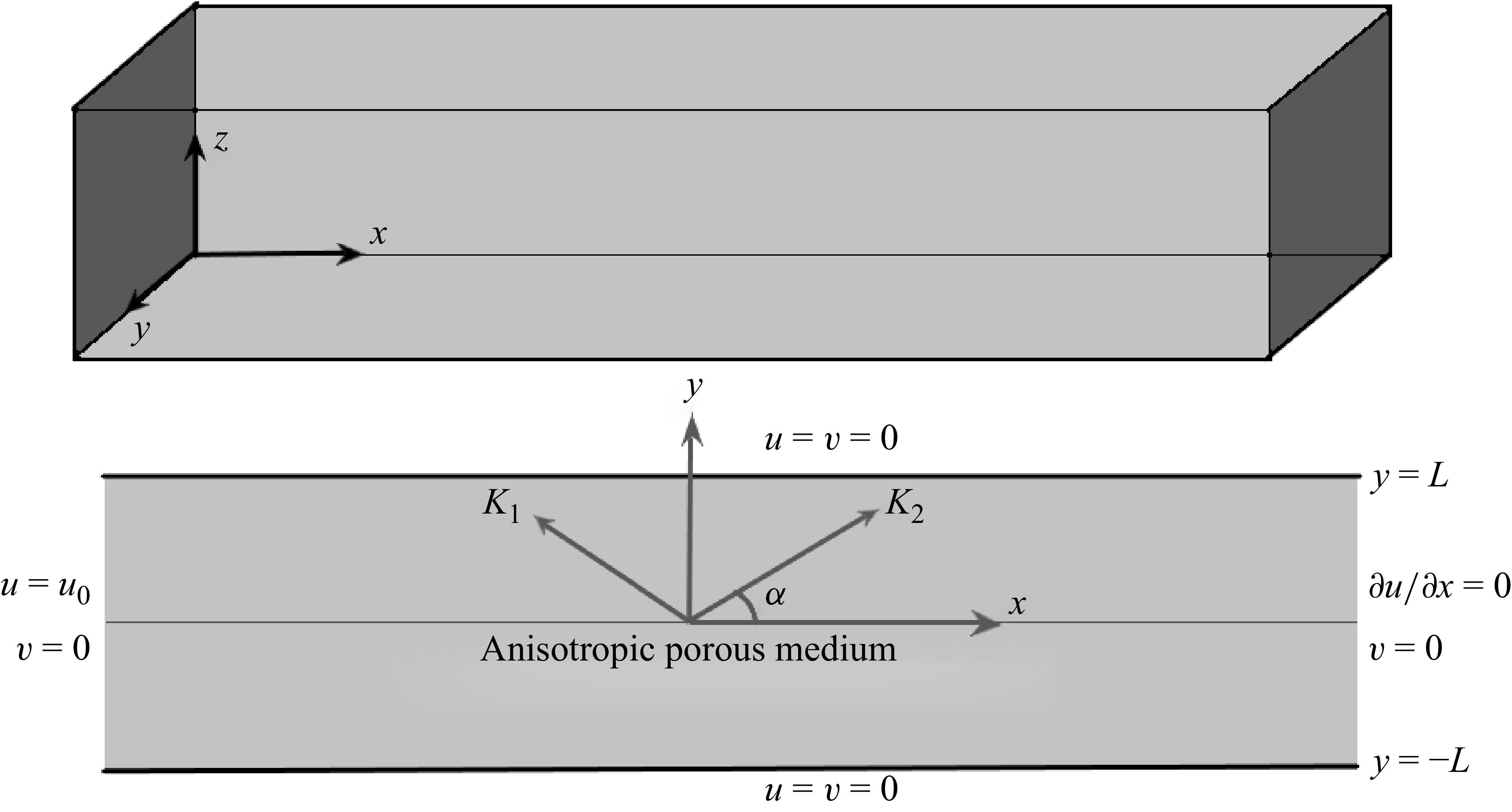
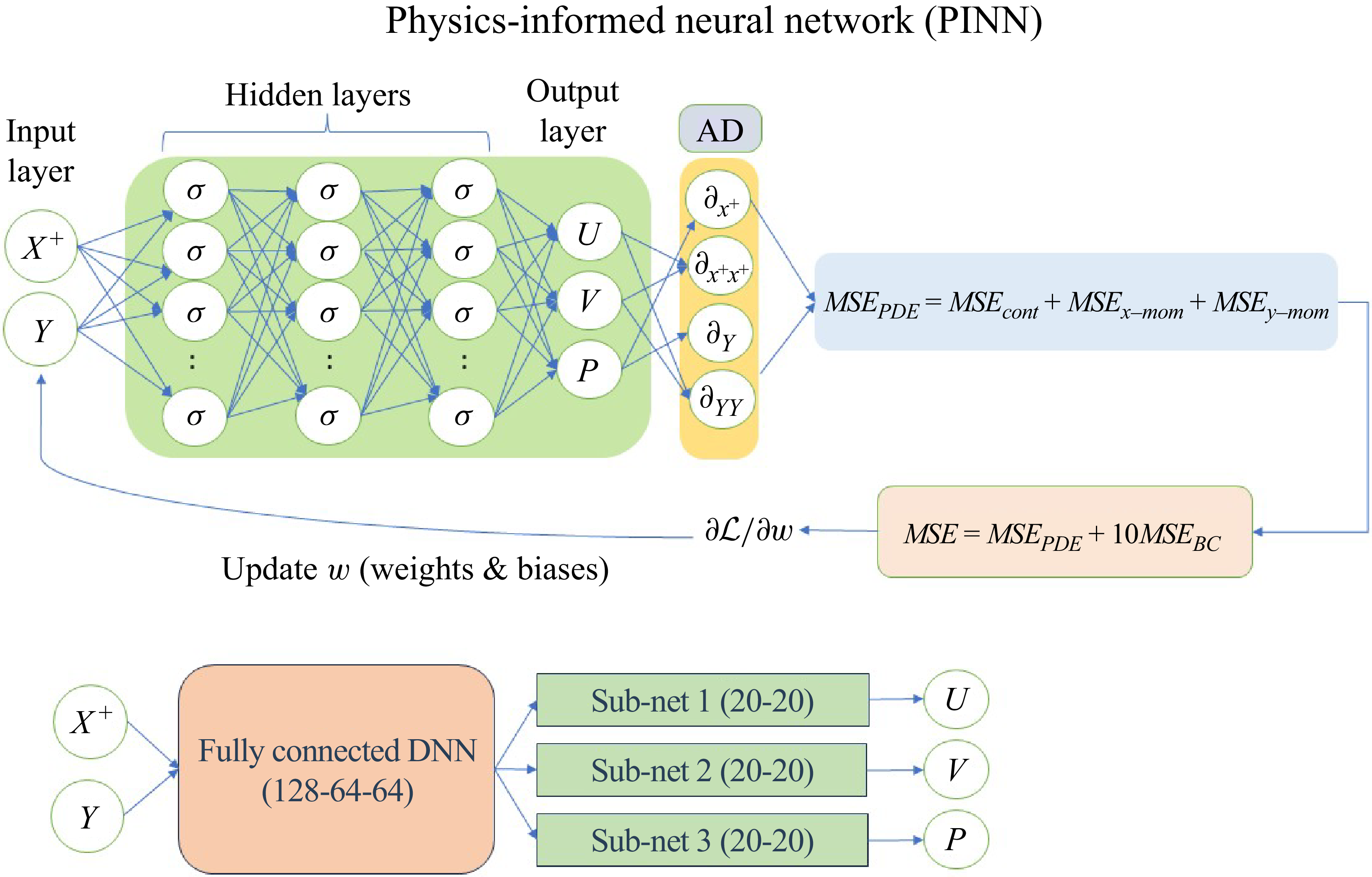
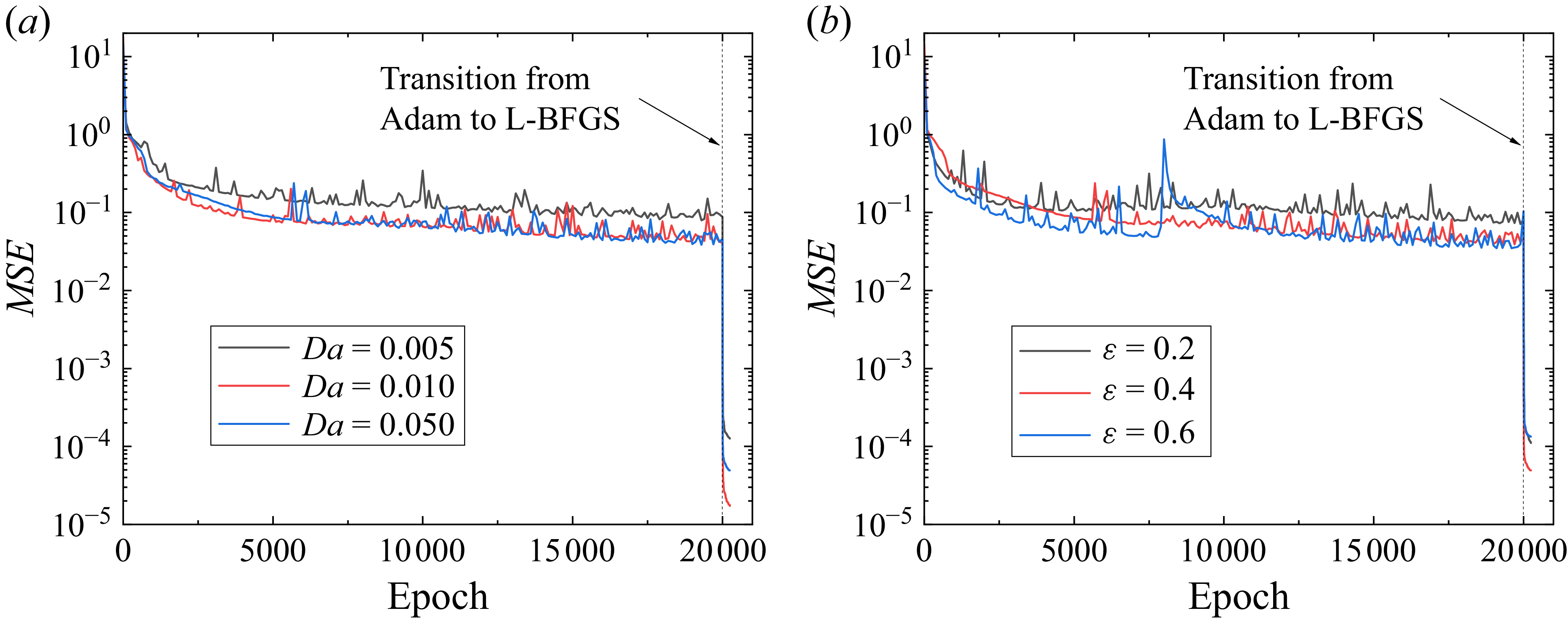
 ϵ
ϵ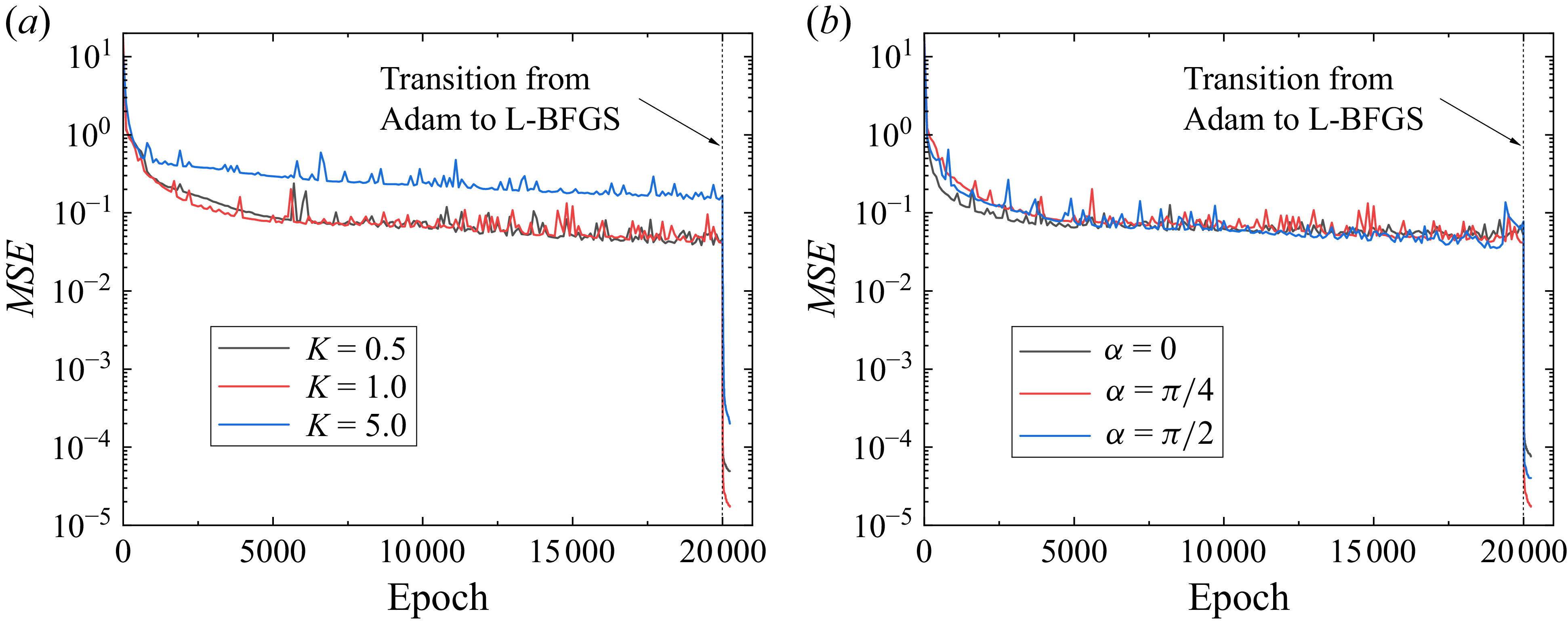
 K
K α
α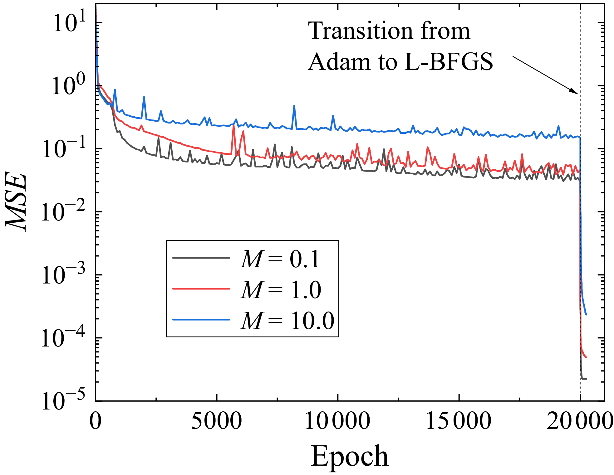
 M
M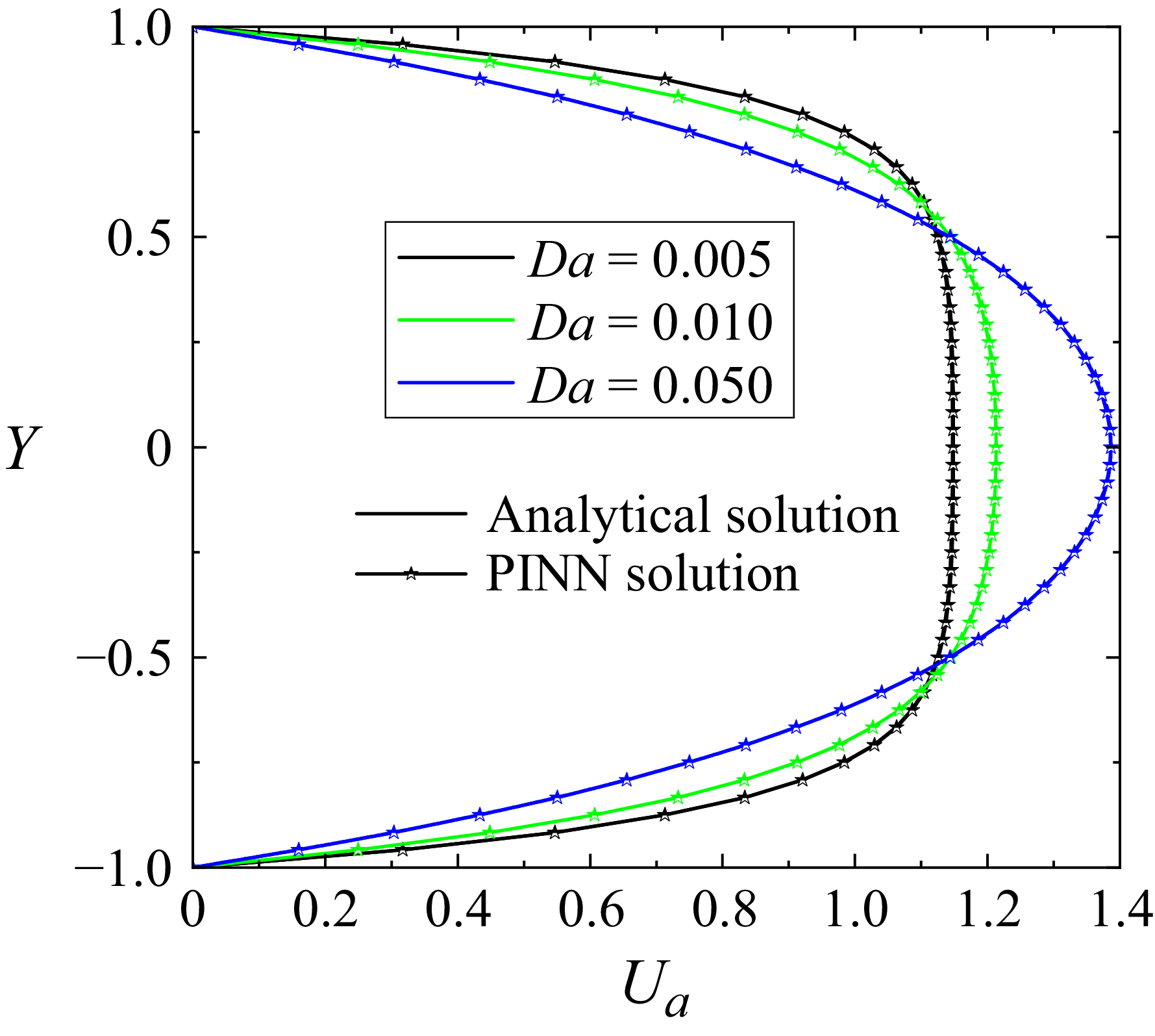
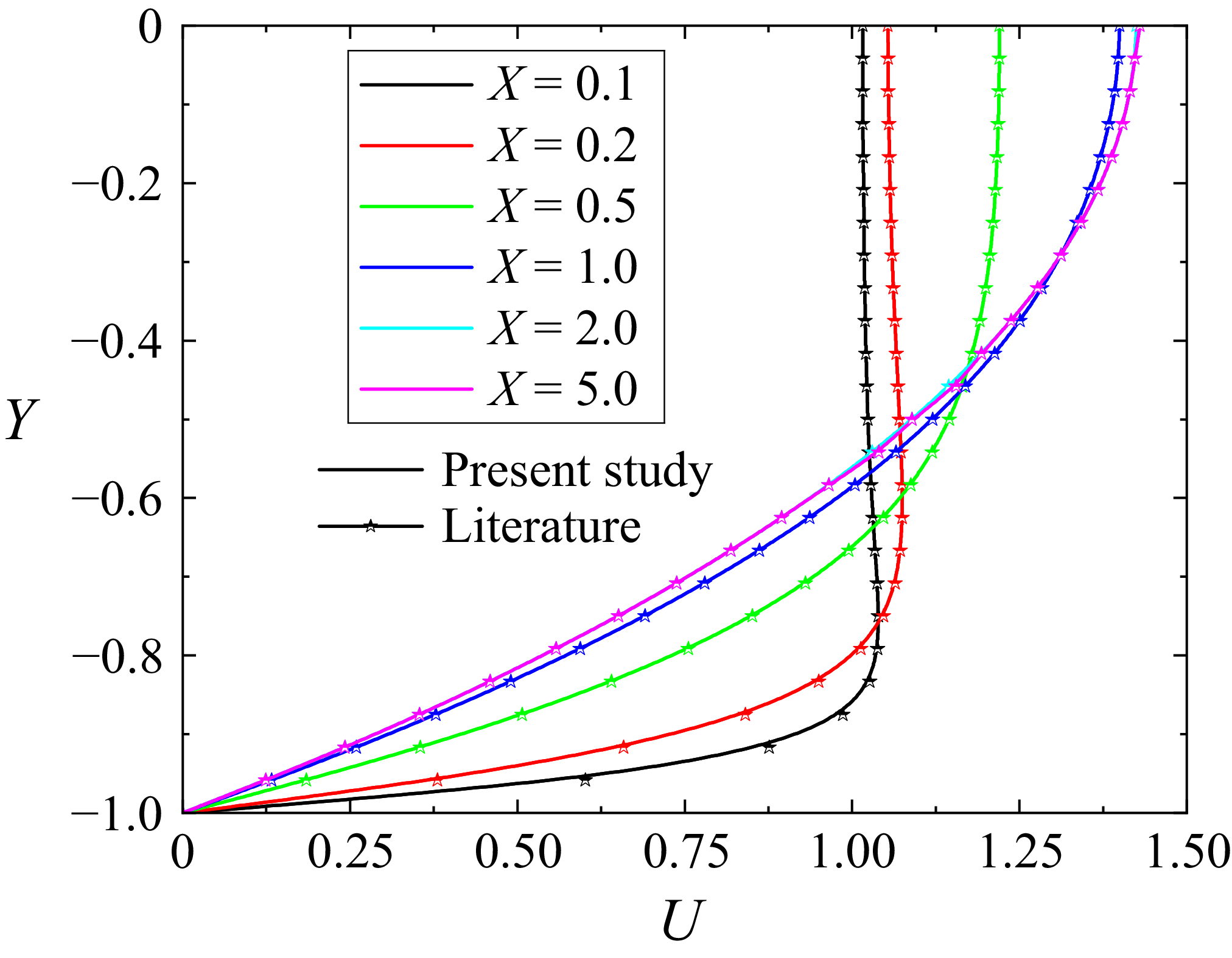
 X+
X+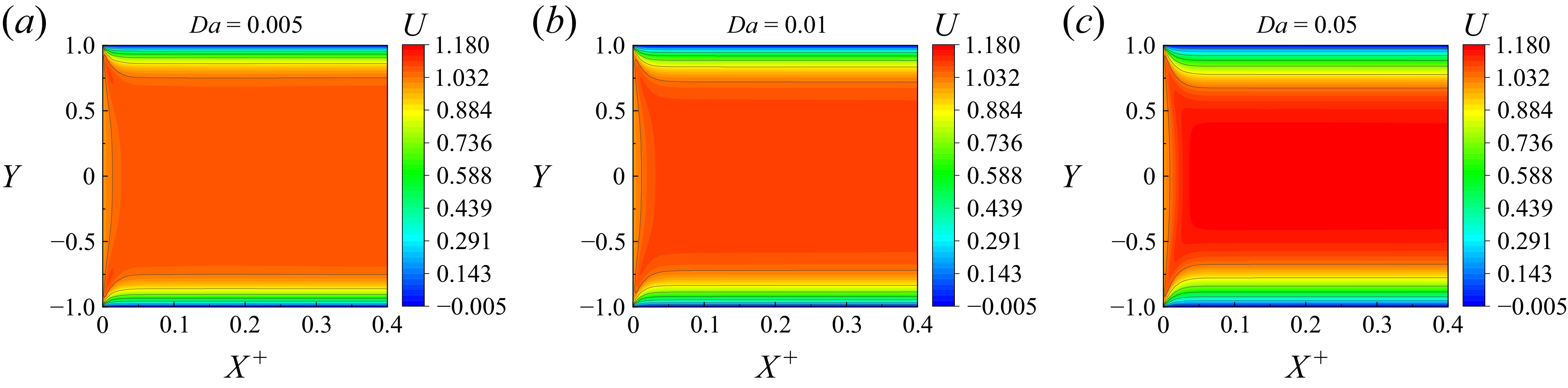
 K=0.5
K=0.5 α=π/4
α=π/4 M=1
M=1 ϵ=0.4
ϵ=0.4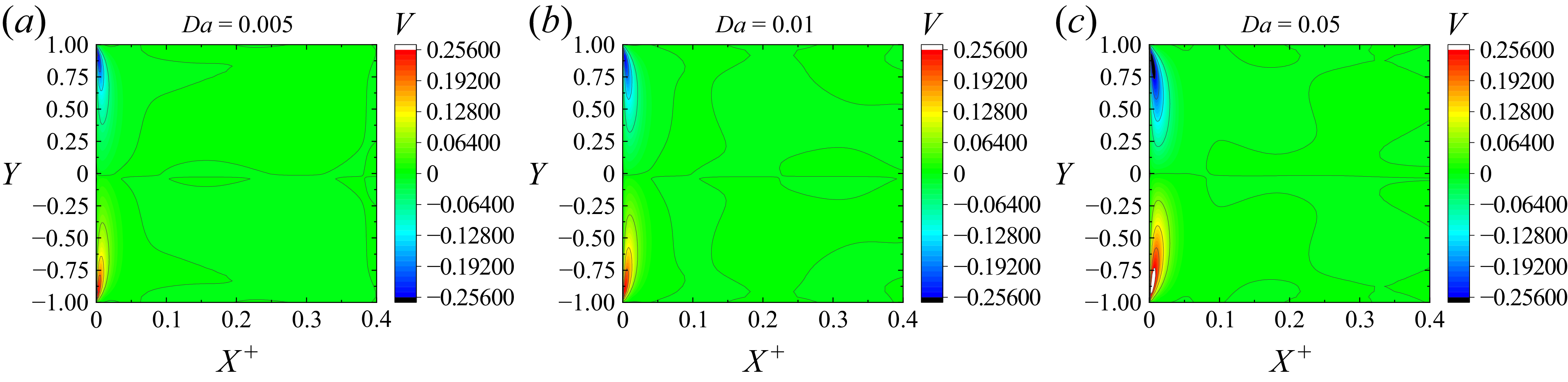
 K=0.5
K=0.5 α=π/4
α=π/4 M=1
M=1 ϵ=0.4
ϵ=0.4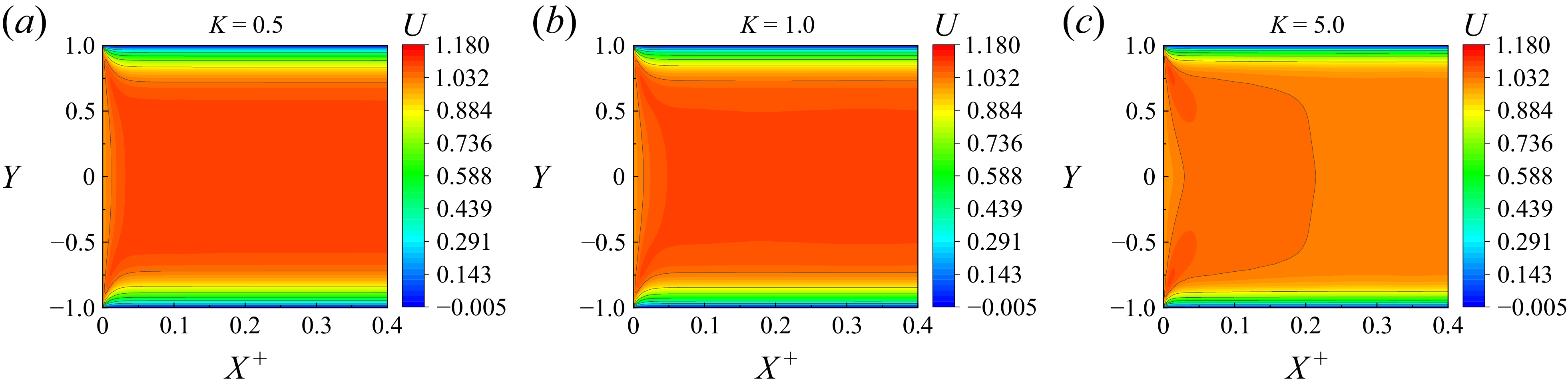
 Da=0.01
 α=π/4
α=π/4 M=1
M=1 ϵ=0.4
ϵ=0.4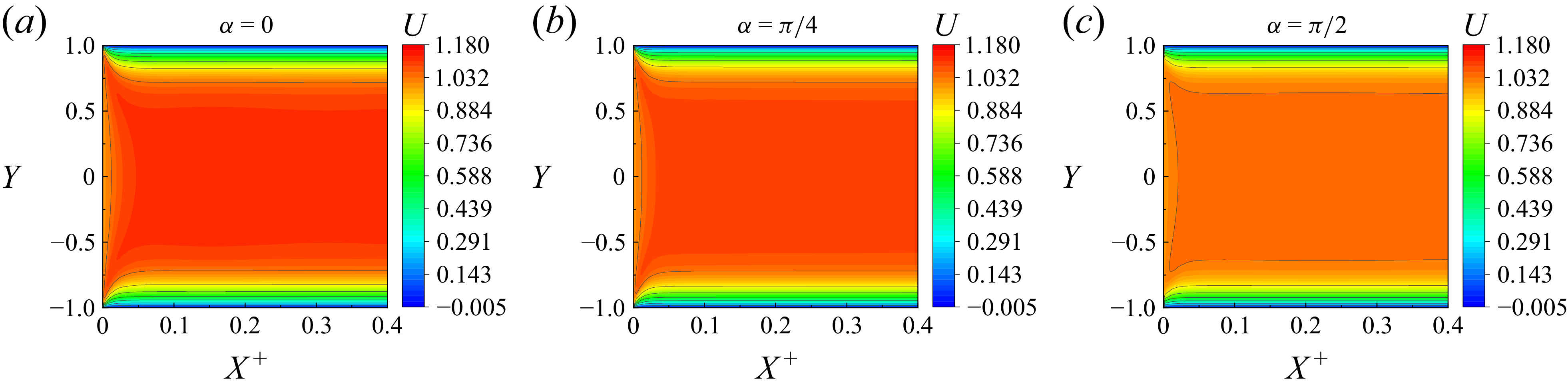
 α
α Da=0.01
 K=0.5
K=0.5 M=1
M=1 ϵ=0.4
ϵ=0.4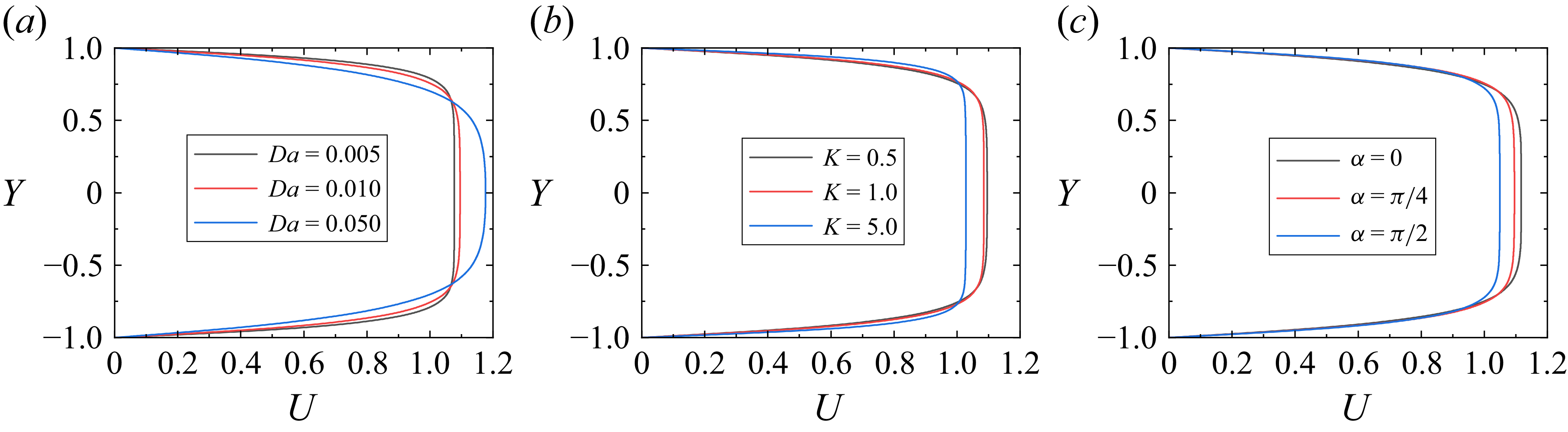
 Da
Da K
K α
α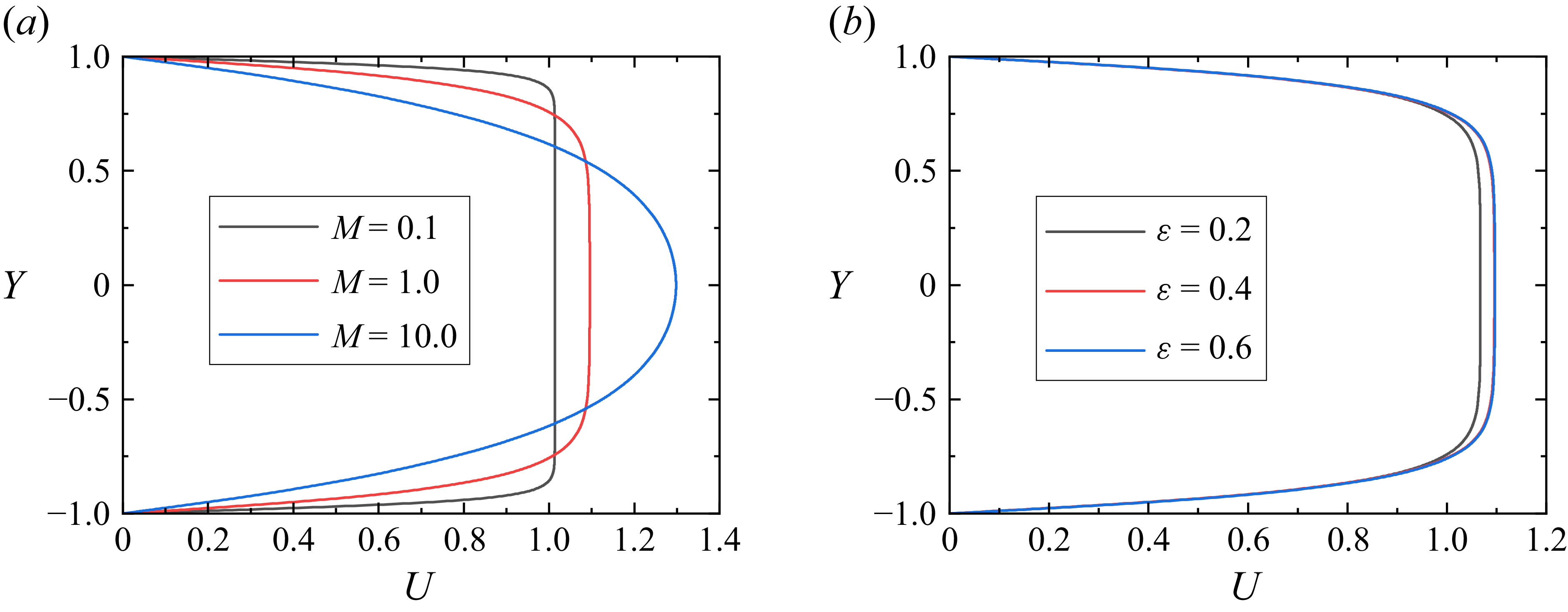
 M
M ϵ
ϵ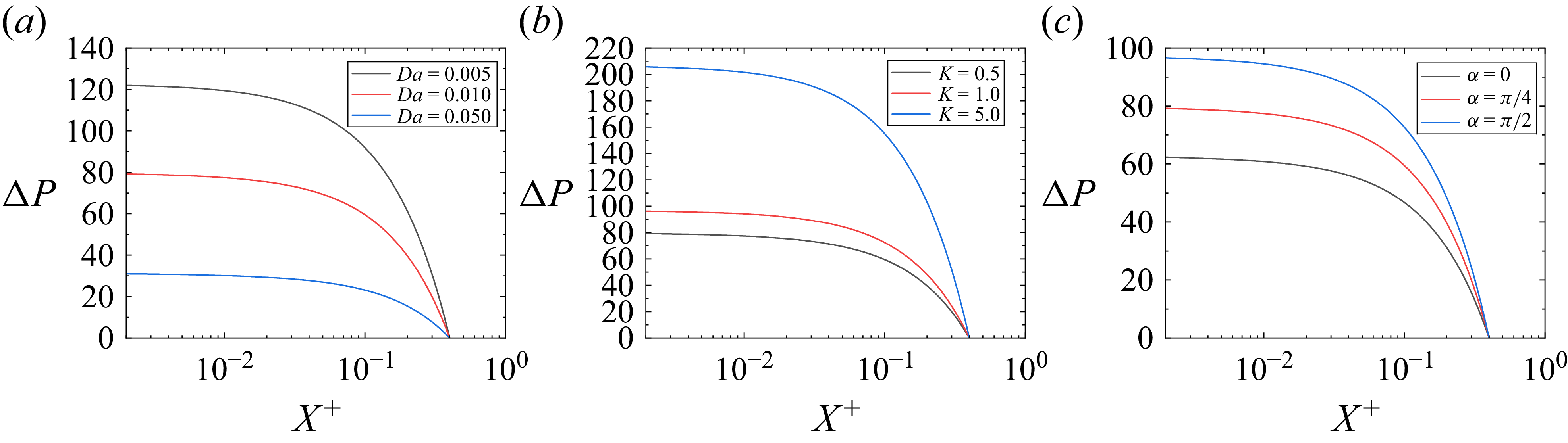
 Da
Da K
K α
α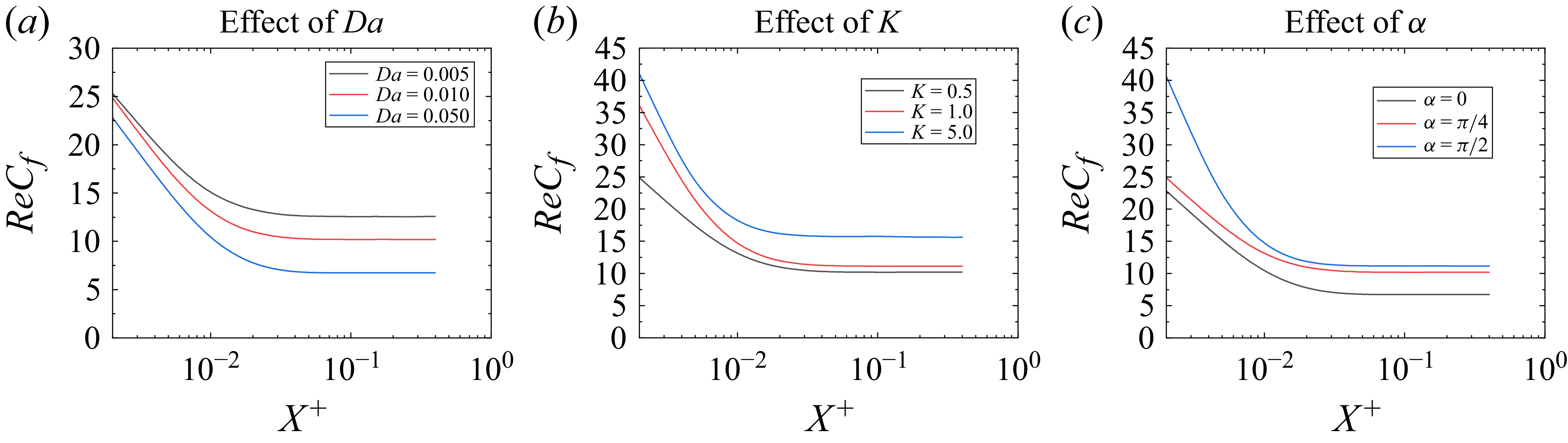
 ReCf
ReCf Da
Da K
K α
α