


1. Introduction
The Lorenz curve is a foundational graphical tool in the study of income distributions, depicting the cumulative share of income received by the bottom  $p$ proportion of the population. A central concept derived from this framework is Lorenz dominance (LD), wherein one distribution is said to dominate another if its Lorenz curve lies entirely above the other’s. This relationship, denoted
  $F \succ_{LD} G$, implies unanimous agreement among all inequality-averse social welfare functionals, as demonstrated by Atkinson [Reference Atkinson2]. Foster and Shorrocks [Reference Foster and Shorrocks13] further showed that LD supports consistent poverty rankings across a wide class of poverty indices sensitive to distributional changes.
Despite its theoretical elegance, strict LD is rarely observed in empirical settings. Empirical Lorenz curves often intersect, rendering binary dominance assessments inconclusive. This empirical reality has motivated the development of statistical procedures to test for LD. Bishop et al. [Reference Bishop, Formby and Smith6, Reference Bishop, Formby and Smith7] initiated this literature with quantile-based inference, which was subsequently refined into pointwise dominance tests by Dardanoni and Forcina [Reference Dardanoni and Forcina9] and Davidson and Duclos [Reference Davidson and Duclos10]. However, Barrett and Donald [Reference Barrett and Donald3] identified size distortions in these methods, leading Barrett et al. [Reference Barrett, Donald and Bhattacharya4] to propose consistent nonparametric approaches grounded in empirical process theory, akin to those employed in stochastic dominance testing. More recently, Sun and Beare [Reference Sun and Beare17] introduced a boundary-corrected bootstrap method that enhances power while maintaining appropriate size.
Alongside inferential advancements, a complementary literature has explored partial and almost dominance frameworks to capture deviations from strict LD. Fishburn and Willig [Reference Fishburn and Willig12] provided formal foundations for partial orderings grounded in transfer principles and social preferences. Duclos et al. [Reference Duclos, Sahn and Younger11] extended these concepts to multidimensional poverty comparisons. Zheng [Reference Zheng20] introduced a formal metric for quantifying almost LD, based on a normalized geometric index denoted as  $\epsilon$. This index is defined as the ratio of the smaller area enclosed between two intersecting Lorenz curves to the total area under the reference Lorenz curve. The measure provides an interpretable gauge of the extent to which one distribution nearly dominates another, even when strict LD does not hold. Chang et al. [Reference Chang, Cheng and Liou8] develop a likelihood-ratio test for LD by framing strict dominance and intersecting curves as nested models. Their method combines maximum likelihood estimation with problem-specific test statistics, but the computational burden increases sharply with each additional crossing point, requiring the use of advanced optimization and simulation techniques.
In this paper, we propose the Lorenz dominance index (LDI), a continuous, population-based metric that quantifies the extent to which one distribution fails to Lorenz dominate another. Unlike existing area-based measures of almost dominance, the LDI focuses on the proportion of the population for which one Lorenz curve lies below the other, offering an interpretable and statistically tractable measure of partial dominance.
A clear distinction must be drawn between area-based inequality measures and dominance-based measures such as the LDI. Standard indices like the Gini coefficient quantify the magnitude of inequality but provide no information about which population segments are relatively better or worse off when comparing two distributions. LD, by contrast, offers this segment-specific insight but does not indicate how large the underlying inequality differences are; strict dominance may arise even when conventional inequality indices differ only marginally. The LDI is therefore introduced to summarize the breadth of (near) LD—that is, the proportion of the population for which one distribution yields relatively better outcomes. Crucially, the LDI does not measure the degree of inequality, and its values should not be interpreted as reflecting large or small inequality differences. Instead, it is a descriptive, non-normative complement to standard inequality indices, highlighting which parts of the population benefit more under one distribution while avoiding conflation between dominance breadth and inequality magnitude.
To support its use in empirical applications, we develop a full statistical framework for the LDI. To support its use in applied research, We derive its asymptotic distribution and establish asymptotic normality under mild regularity conditions, thereby enabling valid statistical inference. To aid practical implementation, we also design a nonparametric bootstrap procedure for constructing confidence intervals and testing hypotheses related to partial LD. Extensive simulation studies demonstrate the estimator’s robustness and efficiency across diverse data-generating processes. Finally, we apply the LDI to Chinese household income data, illustrating its empirical relevance and utility in real-world distributional analysis.
The remainder of this paper is structured as follows: Section 2 presents the estimation procedure for the LDI and outlines its asymptotic properties. Section 3 introduces the bootstrap methodology for inference. Section 4 reports simulation results evaluating the performance of the estimator. Section 5 provides an empirical analysis based on household income data from China. Proofs of the main theoretical results are provided in the Appendix.
2. Lorenz dominance index: estimation and statistical properties
This section introduces the LDI as a population-based measure for comparing income distributions and assessing inequality dominance. We begin by defining the LDI and discussing its interpretability and relevance in distributional analysis. We then present an empirical estimation framework suitable for practical implementation, followed by a detailed examination of the estimator’s asymptotic properties under standard regularity conditions. Together, these components provide a rigorous foundation for statistical inference using the LDI in applied settings.
2.1. Definition and interpretation of the Lorenz dominance index
Let  $F_1:[0, \infty) \to [0, 1]$ and
  $F_2:[0, \infty) \to [0, 1]$ denote the cumulative distribution functions (CDFs) of two income (or wealth) distributions. We impose the following regularity conditions.
Assumption 2.1. For each  $j \in \{1,2\}$,
  $F_j(0)=0$,
  $F_j$ is continuously differentiable with strictly positive density
  $f_j$ on its support, and possesses a finite absolute moment of order
  $(2+\epsilon)$ for some
  $\epsilon \gt 0$.
Given Assumption 2.1, we define the Lorenz curves  $L_j$ for
  $j=1,2$, as
 \begin{equation*}
L_j(p) = \frac{1}{\mu_j}\int_{0}^{p} Q_j(t) \, {\rm dt} \quad \text{for } p \in [0,1],
\end{equation*}
\begin{equation*}
L_j(p) = \frac{1}{\mu_j}\int_{0}^{p} Q_j(t) \, {\rm dt} \quad \text{for } p \in [0,1],
\end{equation*} where  $Q_j(p) = \inf \{x: F_j(x) \geq p,\; x\in [0,\infty)\}$ represents the quantile function, and
  $\mu_j=\int_0^{\infty} t f_j(t) \, {\rm dt}$ denotes the mean of distribution
  $F_j$. The condition for the LD of distribution
  $F_1$ over
  $F_2$ is satisfied if and only if
  $L_1(p) \geq L_2(p)$ for all
  $p \in [0,1]$, where the Lorenz curve
  $L(p)$ represents the cumulative share of total income earned by the bottom
  $p$ proportion of the population. In this framework, if
  $L_1(p) \gt L_2(p)$ for some
  $p$, it implies that the poorest
  $p$ fraction of population 1 holds a larger share of total income than the corresponding fraction in population 2, indicating relatively greater equality in
  $F_1$ at that quantile.
In many empirical applications, Lorenz curves intersect, indicating that neither distribution fully dominates the other. In such cases, the binary LD criterion is inconclusive, as it cannot establish which distribution exhibits greater inequality. To address this limitation, we propose a continuous measure known as the LDI, which quantifies the extent to which the LD condition is violated. This measure enables more nuanced and informative comparisons between income distributions.
The LDI is formally defined as:
 \begin{equation*}
\Gamma(F_1, F_2) = \mu\left\{p: L_1(p) \lt L_2(p),\; p\in (0, 1) \right\},
\end{equation*}
\begin{equation*}
\Gamma(F_1, F_2) = \mu\left\{p: L_1(p) \lt L_2(p),\; p\in (0, 1) \right\},
\end{equation*} where  $\mu$ denotes the Lebesgue measure on
  $(0,1)$. That is,
  $\Gamma(F_1, F_2)$ measures the proportion of the population over which the Lorenz curve of
  $F_1$ fails to Lorenz dominate
  $F_2$.
The LDI has several desirable properties. It satisfies the bounds  $0 \le \Gamma(F_1, F_2) \le 1$, where:
•
 $ \Gamma(F_1, F_2) = 0 $ implies LD of
$ F_1 $ over
$ F_2 $,
$ \Gamma(F_1, F_2) = 0 $ implies LD of
$ F_1 $ over
$ F_2 $,•
$ \Gamma(F_1, F_2) = 1 $ implies LD in the opposite direction, i.e., of
$ F_2 $ over
$ F_1 $,•
$ \Gamma(F_1, F_2) = 0.5 $ implies that the two distributions are symmetric with respect to LD, indicating no clear dominance by either in terms of inequality.


Moreover, the LDI satisfies a natural symmetry property:
 \begin{equation*}
\Gamma(F_1, F_2) = 1 - \Gamma(F_2, F_1).
\end{equation*}
\begin{equation*}
\Gamma(F_1, F_2) = 1 - \Gamma(F_2, F_1).
\end{equation*} This symmetry allows for direct comparison: when  $\Gamma(F_1, F_2) \lt \Gamma(F_2, F_1) $, the Lorenz curve of
  $F_1$ lies below that of
  $F_2$ over a smaller proportion of the population, indicating that
  $F_1$ exhibits less inequality relative to
  $F_2$. Specifically, values of
  $\Gamma(F_1, F_2)$ below 0.5 suggest that
  $F_1$ is less unequal compared to
  $F_2$, while values above 0.5 suggest the opposite.
In contrast to the  $\epsilon$-index introduced by Zheng [Reference Zheng20], which quantifies inequality deviation by measuring the area between intersecting Lorenz curves, the LDI offers a population-based alternative. Rather than focusing on the intensity of deviation, the LDI measures the proportion of the population for which one distribution’s Lorenz curve lies below another’s, highlighting the breadth of deviation from LD.
This perspective aligns more closely with how inequality affects people across a society. Intensity-based measures like the  $\epsilon$-index may emphasize sharp deviations in narrow segments of the population, potentially overlooking broader, more pervasive differences. In contrast, the LDI captures how many people are impacted by inequality, making it more intuitive and relevant for policy design and evaluation
2.2. Illustrative example of partial Lorenz dominance
To illustrate the type of situations where the LDI is most informative, we construct two plausible income distributions for populations A and B using a standard spliced model. In this model, the bottom 90% follows a Lognormal distribution and the top 10% follows a Pareto tail—a widely used approach to approximate real-world income distributions. Population A is specified by
 \begin{equation*}
\mu_A = 0.6, \quad \sigma_A = 1.2, \quad \alpha_A = 1.7,
\end{equation*}
\begin{equation*}
\mu_A = 0.6, \quad \sigma_A = 1.2, \quad \alpha_A = 1.7,
\end{equation*}while Population B has a more dispersed Lognormal body and a lighter Pareto tail:
 \begin{equation*}
\sigma_B = 1.6, \quad \alpha_B = 4.34,
\end{equation*}
\begin{equation*}
\sigma_B = 1.6, \quad \alpha_B = 4.34,
\end{equation*} with  $\mu_B = 0.54$ calibrated so that both distributions share the same mean income (
 $\approx 4.05$). These parameter choices reflect realistic patterns in which middle-class dispersion and top-income behavior differ across populations. The resulting Lorenz curves intersect at
  $p = 0.77$ (Figure 1). Although the Gini coefficients are nearly identical (
 $\approx 0.634$), the underlying distributional differences are substantial. Area-based measures, which weight the magnitude of vertical gaps between curves, may favor Population B because the area where
  $L_B \gt L_A$ slightly exceeds the reverse:
 \begin{equation*}
\int_0^p [L_A(q) \gt L_B(q)]\, dq \approx 0.0105, \quad
\int_p^1 [L_B(q) \gt L_A(q)]\, dq \approx 0.0156.
\end{equation*}
\begin{equation*}
\int_0^p [L_A(q) \gt L_B(q)]\, dq \approx 0.0105, \quad
\int_p^1 [L_B(q) \gt L_A(q)]\, dq \approx 0.0156.
\end{equation*}The Lorenz curves of the populations A and B, represented by  $L_1$ (orange curve) and
  $L_2$ (blue curve), respectively.

Figure 1 Long description
The x-axis label is Cumulative Population Share (p). The x-axis ranges from 0 percent to 100 percent, with tick labels at 0 percent, 10 percent, 20 percent, 30 percent, 40 percent, 50 percent, 60 percent, 70 percent, 80 percent, 90 percent and 100 percent. The y-axis label is Cumulative Income Share L(p). The y-axis ranges from 0 percent to 100 percent, with tick labels at 0 percent, 25 percent, 50 percent, 75 percent and 100 percent. A legend titled Group lists two entries: Population A and Population B. A text box states: Group A and B: Mean equals 4.05 Gini equals 0.634. A dashed diagonal line runs from (0 percent, 0 percent) to (100 percent, 100 percent). Two curves start at (0 percent, 0 percent) and end at (100 percent, 100 percent). A vertical dotted line is drawn at 80 percent on the x-axis. A label near the curves states: Intersection p equals 0.77. Two area annotations are shown: Area: L subscript A minus L subscript B approximately equal to 0.0105 and Area: L subscript B minus L subscript A approximately equal to 0.0156.
This occurs because differences in the top 23% dominate the integrated area, potentially obscuring patterns that affect the majority of the population. The LDI, in contrast, focuses on the breadth of LD by measuring the proportion of the population for which one Lorenz curve lies above the other:
 \begin{equation*}
\begin{aligned}
\Gamma(F_A, F_B) &= \mu\{q : L_A(q) \lt L_B(q)\} = 1-p \approx 0.23, \\
\Gamma(F_B, F_A) &= \mu\{q : L_B(q) \lt L_A(q)\} = p \approx 0.77.
\end{aligned}
\end{equation*}
\begin{equation*}
\begin{aligned}
\Gamma(F_A, F_B) &= \mu\{q : L_A(q) \lt L_B(q)\} = 1-p \approx 0.23, \\
\Gamma(F_B, F_A) &= \mu\{q : L_B(q) \lt L_A(q)\} = p \approx 0.77.
\end{aligned}
\end{equation*}From this perspective, population A clearly dominates for most of the population. This example highlights the policy-relevant advantage of LDI: it captures broad population-level patterns, complementing area-based measures, which may overemphasize differences in small segments such as the top tail.
2.3. Empirical estimation framework
We construct empirical estimators of the LDI using independent random samples from the distributions  $F_1$ and
  $F_2$. Let
  $\{X_i^j\}_{i=1}^{n_j} \stackrel{\text{i.i.d.}}{\sim} F_j$ for
  $j=1,2$ denote two independent samples. Based on these, we define the empirical distribution function, sample mean, and empirical quantile function for each sample as follows:
 \begin{equation*}
\begin{aligned}
\hat{F}_j(x) &= \frac{1}{n_j} \sum_{i=1}^{n_j} \mathbb{I}_{\{X_i^j \leq x\}}, \\
\hat{\mu}_j &= \frac{1}{n_j} \sum_{i=1}^{n_j} X_i^j, \\
\hat{Q}_j(p) &= \inf\left\{x \geq 0 : \hat{F}_j(x) \geq p\right\}, \quad p \in [0,1].
\end{aligned}
\end{equation*}
\begin{equation*}
\begin{aligned}
\hat{F}_j(x) &= \frac{1}{n_j} \sum_{i=1}^{n_j} \mathbb{I}_{\{X_i^j \leq x\}}, \\
\hat{\mu}_j &= \frac{1}{n_j} \sum_{i=1}^{n_j} X_i^j, \\
\hat{Q}_j(p) &= \inf\left\{x \geq 0 : \hat{F}_j(x) \geq p\right\}, \quad p \in [0,1].
\end{aligned}
\end{equation*}Subsequently, the Lorenz curve estimator for each distribution is given by:
 \begin{equation*}
\hat{L}_j(p) = \hat{\mu}_j^{-1}\int_0^p \hat{Q}_j(t)\mathrm{d}t,\quad j=1,2,
\end{equation*}
\begin{equation*}
\hat{L}_j(p) = \hat{\mu}_j^{-1}\int_0^p \hat{Q}_j(t)\mathrm{d}t,\quad j=1,2,
\end{equation*}which, in turn, defines the estimator of the LDI as:
 \begin{equation*}
\hat{\Gamma} = \Gamma(\hat{F}_1,\hat{F}_2) = \mu\left\{p \in (0,1) : \hat{L}_1(p) \lt \hat{L}_2(p)\right\},
\end{equation*}
\begin{equation*}
\hat{\Gamma} = \Gamma(\hat{F}_1,\hat{F}_2) = \mu\left\{p \in (0,1) : \hat{L}_1(p) \lt \hat{L}_2(p)\right\},
\end{equation*} where  $\mu$ denotes the Lebesgue measure on the unit interval. This index represents the proportion of the population for which the empirical Lorenz curve of
  $F_1$ lies below that of
  $F_2$, thereby reflecting the extent of inequality dominance.
For practical computation, we approximate  $\hat{\Gamma}$ via numerical integration using a discretization of the unit interval. Let
  $\mathcal{T}_M = \{t_i\}_{i=1}^M$ be a grid of
  $M$ equally spaced points in
  $(0,1)$, with
  $t_i = i/(M+1)$ and typically
  $M=1000$. Then, the empirical approximation becomes:
 \begin{equation*}
\hat{\Gamma} = (M+1)^{-1}\sum_{i=1}^M \mathbb{I}_{\{\hat{L}_1(t_i) \lt \hat{L}_2(t_i)\}},
\end{equation*}
\begin{equation*}
\hat{\Gamma} = (M+1)^{-1}\sum_{i=1}^M \mathbb{I}_{\{\hat{L}_1(t_i) \lt \hat{L}_2(t_i)\}},
\end{equation*}which estimates the proportion of grid points where the Lorenz curve of sample 1 lies below that of sample 2. This proportion serves as a consistent estimator of the population-based LDI and forms the basis for subsequent asymptotic analysis.
2.4. Asymptotic properties of the estimator
This subsection examines the asymptotic properties of the proposed estimator under additional regularity conditions.
Assumption 2.2. Let  $n=n_1n_2/(n_1+n_2)$. As
  $n_1, n_2 \to \infty$, we have
  $n \to \infty$ and the proportion
  $\frac{n_1}{n_1 + n_2} \to \lambda$ for some constant
  $\lambda \in (0, 1)$.
Assumption 2.3. There exists a finite number of  $p$ values such that
  $L_1(p) = L_2(p)$ but
  $Q_1(p)/\mu_1 \not= Q_2(p)/\mu_2$. In addition, suppose that
 \begin{equation}
\lim\limits_{p\rightarrow0} \frac{Q_1(p)\mu_2}{Q_2(p)\mu_1} \not=1,~~ \lim\limits_{p\rightarrow1} \frac{Q_1(p)\mu_2}{Q_2(p)\mu_1} \not=1.
\end{equation}
\begin{equation}
\lim\limits_{p\rightarrow0} \frac{Q_1(p)\mu_2}{Q_2(p)\mu_1} \not=1,~~ \lim\limits_{p\rightarrow1} \frac{Q_1(p)\mu_2}{Q_2(p)\mu_1} \not=1.
\end{equation}Theorem 2.4 Under Assumptions 2.1–2.3, as  $n \to \infty$,
 \begin{equation*}
\sqrt{n} \left( \hat{\Gamma} - \Gamma(F_1, F_2) \right) \xrightarrow{d} \text{N}(0, \sigma^2)
\end{equation*}
\begin{equation*}
\sqrt{n} \left( \hat{\Gamma} - \Gamma(F_1, F_2) \right) \xrightarrow{d} \text{N}(0, \sigma^2)
\end{equation*} for some asymptotic variance  $\sigma^2$. In particular:
(i) If  $L_1$ and
  $L_2$ have no crossing point, then
  $\hat{\Gamma}-\Gamma(F_1,F_2) = \boldsymbol{o}_p(n^{-1/2}), i.e., \sigma^2 = 0$.
(ii) If  $L_1$ and
  $L_2$ have exactly one crossing point at
  $p=p_1^\ast$, then
 \begin{equation}
\sigma^2=\tau^2(p^\ast_1)\Big[\frac{\lambda p_1^\ast(1-p_1^\ast)}{f^2_1(Q_1(p_1^\ast))\mu_1^2}+\frac{(1-\lambda) p_1^\ast(1-p_1^\ast)}{f^2_2(Q_2(p_1^\ast))\mu_2^2}\Big];
\end{equation}
\begin{equation}
\sigma^2=\tau^2(p^\ast_1)\Big[\frac{\lambda p_1^\ast(1-p_1^\ast)}{f^2_1(Q_1(p_1^\ast))\mu_1^2}+\frac{(1-\lambda) p_1^\ast(1-p_1^\ast)}{f^2_2(Q_2(p_1^\ast))\mu_2^2}\Big];
\end{equation} (iii) If  $L_1$ and
  $L_2$ have exactly two crossing points
  $p_1^\ast \lt p_2^\ast$, then
 \begin{equation*}\sigma^2=\tau^2(p^\ast_1)\left[\frac{\lambda p_1^\ast(1-p_1^\ast)}{f^2_1(Q_1(p_1^\ast))\mu_1^2}+\frac{(1-\lambda) p_1^\ast(1-p_1^\ast)}{f^2_2(Q_2(p_1^\ast))\mu_2^2}\right]\end{equation*}
 \begin{equation*}+\tau^2(p^\ast_2)\left[\frac{\lambda p_2^\ast(1-p_2^\ast)}{f^2_1(Q_1(p_2^\ast))\mu_1^2}+\frac{(1-\lambda) p_2^\ast(1-p_2^\ast)}{f^2_2(Q_2(p_2^\ast))\mu_2^2}\right]\end{equation*}
 \begin{equation}
-2\tau(p^\ast_1)\tau(p^\ast_2)\left[\frac{\lambda p_1^\ast(1-p_2^\ast)}{f^2_1(Q_1(p_1^\ast))\mu_1^2}+\frac{(1-\lambda) p_1^\ast(1-p_2^\ast)}{f^2_2(Q_2(p_1^\ast))\mu_2^2}\right],
\end{equation}
\begin{equation}
-2\tau(p^\ast_1)\tau(p^\ast_2)\left[\frac{\lambda p_1^\ast(1-p_2^\ast)}{f^2_1(Q_1(p_1^\ast))\mu_1^2}+\frac{(1-\lambda) p_1^\ast(1-p_2^\ast)}{f^2_2(Q_2(p_1^\ast))\mu_2^2}\right],
\end{equation} where  $\tau(p)=f_1(Q_1(p))f_2(Q_2(p))/\left[\mu_1f_2(Q_2(p))-\mu_2f_1(Q_1(p))\right]$.
3. Bootstrap-based inference
3.1. Asymptotic properties and bootstrap validity
A rigorous asymptotic analysis of point estimators requires careful evaluation of estimation error, particularly to support the construction of confidence intervals and the implementation of hypothesis testing procedures. While Theorem 2.4 provides the asymptotic variance of the estimator, it depends on unknown features of the underlying population distributions, limiting its direct applicability. To address this issue, we advocate the use of bootstrap methods, which offer a practical and flexible approach to approximating the sampling distribution of the estimator without requiring explicit knowledge of the data-generating process.
Let  $\{X_i^1\}_{i=1}^{n_1}$ and
  $\{X_i^2\}_{i=1}^{n_2}$ denote independent samples drawn from distributions
  $F_1$ and
  $F_2$, respectively. For each
  $b = 1, \ldots, B$, we independently generate bootstrap samples
  $\{X_i^{1\ast b}\}_{i=1}^{n_1}$ and
  $\{X_i^{2\ast b}\}_{i=1}^{n_2}$ by resampling with replacement from the original data. The empirical distribution functions and corresponding quantile functions are then defined as
 \begin{equation*}
\hat{F}^{\ast b}_j(x) = \frac{1}{n_j} \sum_{i=1}^{n_j} \mathbb{I}_{\{X_i^{j\ast b} \leq x\}}, \quad x \in [0,\infty), \quad j = 1,2,
\end{equation*}
\begin{equation*}
\hat{F}^{\ast b}_j(x) = \frac{1}{n_j} \sum_{i=1}^{n_j} \mathbb{I}_{\{X_i^{j\ast b} \leq x\}}, \quad x \in [0,\infty), \quad j = 1,2,
\end{equation*}and
 \begin{equation*}
\hat{Q}^{\ast b}_j(p) = \inf \{x \in [0, \infty): \hat{F}^{\ast b}_j(x) \geq p\}, \quad p \in [0,1].
\end{equation*}
\begin{equation*}
\hat{Q}^{\ast b}_j(p) = \inf \{x \in [0, \infty): \hat{F}^{\ast b}_j(x) \geq p\}, \quad p \in [0,1].
\end{equation*} The bootstrap estimators of the Lorenz curves and the functional  $\Gamma(F_1, F_2)$ are given by
 \begin{equation*}
\hat{L}^{\ast b}_j(p) = \frac{1}{\hat{\mu}^{\ast b}_j}\int_{0}^{p} \hat{Q}^{\ast b}_j(t) \, {\rm dt}\end{equation*}
\begin{equation*}
\hat{L}^{\ast b}_j(p) = \frac{1}{\hat{\mu}^{\ast b}_j}\int_{0}^{p} \hat{Q}^{\ast b}_j(t) \, {\rm dt}\end{equation*}and
 \begin{equation*}\hat{\Gamma}^{\ast b} =\Gamma(\hat{F}^{\ast b}_1,\hat{F}^{\ast b}_2)=\mu\{p: \hat{L}^{\ast b}_1(p) \lt \hat{L}^{\ast b}_2(p),\; p \in (0, 1)\},\end{equation*}
 where  $\hat{\mu}^{\ast b}_j = \frac{1}{n_j} \sum_{i=1}^{n_j} X_i^{j\ast b}$. The empirical distribution of
  $\hat{\Gamma}^{\ast b}$, for
  $b \!=\! 1, \ldots, B$, is then utilized to approximate the distribution of
  $\hat{\Gamma}$. The validity of this approximation is underpinned by the following theorem.
Theorem 3.1 Under Assumptions 2.1–2.3, as  $n \to \infty$,
 \begin{equation*}
\sup_{x} \left| \mathrm{P}^\ast \left( n^{1/2} (\hat{\Gamma}^{\ast b} - \hat{\Gamma}) \le x \right)
- \mathrm{P} \left( n^{1/2} (\hat{\Gamma} - \Gamma) \le x \right) \right| = \boldsymbol{o}_p(1),
\end{equation*}
\begin{equation*}
\sup_{x} \left| \mathrm{P}^\ast \left( n^{1/2} (\hat{\Gamma}^{\ast b} - \hat{\Gamma}) \le x \right)
- \mathrm{P} \left( n^{1/2} (\hat{\Gamma} - \Gamma) \le x \right) \right| = \boldsymbol{o}_p(1),
\end{equation*} where  $\mathrm{P}^\ast$ denotes the conditional probability given the original samples
  $\{X_i^1\}_{i=1}^{n_1}$ and
  $\{X_i^2\}_{i=1}^{n_2}$.
3.2. Bootstrap confidence intervals and hypothesis testing
For a given  $\alpha \in (0, 1/2]$, confidence intervals for
  $\Gamma(F_1, F_2)$ at level
  $1 - \alpha$ can be constructed using the
  $\alpha$-quantiles of the empirical distribution of
  $\hat{\Gamma}^{\ast b} - \hat{\Gamma}$, denoted by
  $z^\ast_\alpha$. Specifically:
 \begin{equation*}
\text{Two-sided interval:} \quad \left[\hat{\Gamma} - z^\ast_{1 - \alpha/2}, \, \hat{\Gamma} - z^\ast_{\alpha/2} \right],
\end{equation*}
\begin{equation*}
\text{Two-sided interval:} \quad \left[\hat{\Gamma} - z^\ast_{1 - \alpha/2}, \, \hat{\Gamma} - z^\ast_{\alpha/2} \right],
\end{equation*} \begin{equation*}
\text{Lower one-sided interval:} \quad \left[\hat{\Gamma} - z^\ast_{1 - \alpha}, \, 1 \right],
\end{equation*}
\begin{equation*}
\text{Lower one-sided interval:} \quad \left[\hat{\Gamma} - z^\ast_{1 - \alpha}, \, 1 \right],
\end{equation*} \begin{equation*}
\text{Upper one-sided interval:} \quad \left[0, \, \hat{\Gamma} - z^\ast_\alpha \right].
\end{equation*}
\begin{equation*}
\text{Upper one-sided interval:} \quad \left[0, \, \hat{\Gamma} - z^\ast_\alpha \right].
\end{equation*} Using these intervals, we may test the following hypotheses for a fixed  $\gamma \in [0, 1]$:
 \begin{align*}
&H_0^1: \Gamma(F_1, F_2) = \gamma, \\
&H_0^2: \Gamma(F_1, F_2) \geq \gamma, \\
&H_0^3: \Gamma(F_1, F_2) \leq \gamma.
\end{align*}
\begin{align*}
&H_0^1: \Gamma(F_1, F_2) = \gamma, \\
&H_0^2: \Gamma(F_1, F_2) \geq \gamma, \\
&H_0^3: \Gamma(F_1, F_2) \leq \gamma.
\end{align*} To interpret these procedures correctly, it is important to distinguish between the true income distributions  $F_1$ and
  $F_2$ and their empirical counterparts
  $\widehat{F}_1$ and
  $\widehat{F}_2$. Bootstrap samples are drawn independently from the original data for each population, and the resulting resamples are used to construct the empirical distributions
  $\widehat{F}_1$ and
  $\widehat{F}_2$, which serve as nonparametric estimators of the underlying distributions. The bootstrap therefore approximates the sampling distribution of
  $\hat{\Gamma}$ under the data-generating processes represented by the empirical distributions, without constructing artificial distributions that impose the restriction
  $\Gamma(F_1, F_2) = \gamma$. Inference proceeds by using the bootstrap distribution of
  $\hat{\Gamma}$ to form confidence intervals for
  $\Gamma(F_1, F_2)$ and to assess whether the hypothesized value
  $\gamma$ lies within these intervals. This approach avoids parametric assumptions and provides valid inference under mild regularity conditions.
The LDI is designed to quantify the extent to which LD holds between two distributions, particularly in cases where their Lorenz curves intersect. Accordingly, hypotheses involving  $\Gamma(F_1, F_2)$ align directly with the interpretive purpose of the index. Although one could alternatively test the stronger hypothesis
  $H_0 : L_1 = L_2$—for example, by pooling the two mean-normalized samples, treating the pooled population as the common null, and drawing two bootstrap subsamples—the null of exact equality of Lorenz curves addresses a distinct question. Such a test concerns full equality of income distributions, whereas the LDI focuses on the breadth of (near) dominance rather than exact equality. For this reason, we focus our inference framework on hypotheses involving
  $\Gamma(F_1, F_2)$.
Given the symmetry  $\Gamma(F_1, F_2) = 1 - \Gamma(F_2, F_1)$, we focus on values of
  $\gamma \in [0, 0.5]$. When
  $\hat{\Gamma}$ is close to zero, the main interest lies in testing whether
  $F_1$ strictly Lorenz-dominates
  $F_2$; i.e.,
  $H_0^1: \Gamma(F_1, F_2) = 0$. In such boundary cases, the convergence of
  $\hat{\Gamma} - \hat{\Gamma}^\ast$ in probability may lead to excessively narrow intervals with undercoverage. To address this, we adjust the bootstrap critical values by setting
 \begin{equation*}
z^\ast_{1 - \alpha} \leftarrow \max\{z^\ast_{1 - \alpha}, \nu\}, \quad
z^\ast_{\alpha} \leftarrow \min\{z^\ast_{\alpha}, -\nu\},
\end{equation*}
\begin{equation*}
z^\ast_{1 - \alpha} \leftarrow \max\{z^\ast_{1 - \alpha}, \nu\}, \quad
z^\ast_{\alpha} \leftarrow \min\{z^\ast_{\alpha}, -\nu\},
\end{equation*} where  $\nu \gt 0$ is a small constant (e.g.,
  $\nu = 0.005$), as used in our simulation study.
When  $\hat{\Gamma} \in (0, 0.5)$, it suggests that
  $F_1$ exhibits a higher degree of equality than
  $F_2$, though not to the extent of strict LD. In this context, we consider testing the hypothesis
  $H_0^2: \Gamma(F_1, F_2) \geq \gamma$ against the alternative
  $H_a^2: \Gamma(F_1, F_2) \lt \gamma$, where
  $\gamma \in (0, 0.5)$ denotes a practically significant threshold. Common choices include
  $\gamma = 0.1$ or
  $\gamma = 0.3$, corresponding to moderate or strong dominance, respectively.
Conversely, when  $\hat{\Gamma}$ is close to
  $0.5$, this suggests that the two distributions exhibit similar levels of inequality. In such cases, we test the null hypothesis
  $H_0^1: \Gamma(F_1, F_2) = 0.5$ as a benchmark for symmetry. Rejection of
  $H_0^1$ indicates a significant asymmetry in inequality between the two distributions. Moreover, rejection of
  $H_0^2$ (or
  $H_0^3$ for
  $F_2$) provides additional evidence that one distribution exhibits lower inequality relative to the other.
4. Monte Carlo simulation
This section is organized into three subsections. First, we evaluate the consistency of our estimator and examine the effectiveness of the proposed bootstrap procedure through Monte Carlo simulations under a range of distributional scenarios. Next, we conduct hypothesis testing for the three proposed hypotheses using various values of  $\gamma$, reflecting different degrees of partial dominance. Finally, we compare the performance of our method with that of [Reference Sun and Beare17], as well as the approach developed by [Reference Barrett, Donald and Bhattacharya4] for testing strict LD.
4.1. Consistency and accuracy of the estimator
To enhance the realism of our simulations, we generate data from the following distributions:  $\text{log-normal LN}(\mu, \sigma^2)$,
  $\text{Pareto Pa}(\alpha, k)$,
  $\text{Weibull W}(a, \sigma)$ (see [Reference Sarabia, Castillo and Slottje16], [Reference Krause14]). Let
  $X^1 \sim F_1$ and
  $X^2 \sim F_2$ denote two independent samples drawn from respective distributions
  $F_1$ and
  $F_2$. Define the true value of the LDI as
  $\Gamma_0 = \Gamma(F_1, F_2)$. We investigate the following scenarios based on different configurations of
  $F_1$ and
  $F_2$:
Case 1.  $X^1\sim \text{LN}(0,0.3^2)$,
  $X^2\sim \text{Pa}(1,3)$;
  $\Gamma_0=0.3853.$
Case 2.  $X^1\sim \text{LN}(0,0.3^2)$,
  $X^2\sim\text{Pa}(1,2.5)$;
 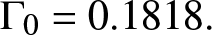 $\Gamma_0=0.1818.$
Case 3.  $X^1\sim \text{Pa}(1,6)$,
  $X^2\sim \text{Pa}(1,3)$;
  $\Gamma_0=0.$
Case 4.  $X^1\sim \text{LN}(0.2,1)$,
  $X^2\sim \text{W}(1,2.7)$;
  $\Gamma_0=0.4473.$
Case 5.  $X^1\sim \text{Pa}(1,2.5)$,
  $X^2\sim \text{LN}(0,0.41^2)$;
  $\Gamma_0=0.5053.$
Case 6.  $X^1\sim \text{LN}(0.2,1^2)$,
  $X^2\sim \text{W}(1,2.7)$;
  $\Gamma_0=0.2869.$
Case 7. In this scenario, we use the illustrative example introduced in Subsection 2.2. Specifically,  $X^1$ and
  $X^2$ are drawn from populations A and B, respectively, and we set the value of
  $\Gamma_0$ to
  $0.23$.
Figures 2, 3, 4 illustrate the Lorenz curves for Cases 1–6, and Figure 1 shows the Lorenz curves for Case 7.
Lorenz curves for  $X^1$ (dashed) and
  $X^2$ (solid) according to Cases 1 and 2.

Figure 2 Long description
Panel A: A multi-line graph comparing Lorenz curves for X superscript 1 (solid line) and X superscript 2 (dashed line). The horizontal axis is labeled p, ranging from 0.0 to 1.0. The vertical axis is labeled L subscript p, ranging from 0.0 to 1.0. At p equals 0.3853, the L subscript p value for X superscript 1 is approximately 0.30, while for X superscript 2 it is slightly lower. Both curves rise from (0.0, 0.0) toward (1.0, 1.0), with X superscript 1 consistently higher. Panel B: A multi-line graph comparing Lorenz curves for X superscript 1 (solid line) and X superscript 2 (dashed line). The horizontal axis is labeled p, ranging from 0.0 to 1.0. The vertical axis is labeled L subscript p, ranging from 0.0 to 1.0. At p equals 0.1818, the L subscript p value for X superscript 1 is approximately 0.12, while for X superscript 2 it is slightly lower. Both curves rise from (0.0, 0.0) toward (1.0, 1.0), with X superscript 1 consistently higher. The graphs illustrate differences in distribution inequality between the two cases, with X superscript 1 showing less inequality in both panels.
Lorenz curves for  $X^1$ (dashed) and
  $X^2$ (solid) according to Cases 3 and 4.

Figure 3 Long description
The image A showing a line graph with a legend listing X superscript 1 and X superscript 2. The horizontal axis label is p, with tick labels 0.0, 0.2, 0.4, 0.6, 0.8, 1.0. The vertical axis label is L subscript p, with tick labels 0.0, 0.2, 0.4, 0.6, 0.8, 1.0. Two curves are plotted: one solid and one dashed. Both curves start near the origin and rise toward the top-right corner. The dashed curve stays above the solid curve across most of the plotted range. The image B showing a line graph with a legend listing X superscript 1 and X superscript 2. The horizontal axis label is p, with tick labels 0.0, 0.2, 0.4, 0.6, 0.8, 1.0. The vertical axis label is L subscript p, with tick labels 0.0, 0.2, 0.4, 0.6, 0.8, 1.0. Two curves are plotted: one solid and one dashed. A numeric annotation on the horizontal axis reads 0.5527. The two curves meet at approximately p equals 0.5527, then separate, with the dashed curve above the solid curve for larger p values.
Lorenz curves for  $X^1$ (dashed) and
  $X^2$ (solid) according to Cases 5 and 6.

Figure 4 Long description
Two line graphs display Lorenz curves for X superscript 1 and X superscript 2, representing inequality distributions. The x-axis is labeled 'p' with no units, ranging from 0 to 1. The y-axis is labeled 'L(p)' with no units, also ranging from 0 to 1. In both graphs, the solid line represents X superscript 2 and the dashed line represents X superscript 1. A) The curves rise from (0,0) to (1,1), with a marked point at approximately (0.4947, 0.3) on the solid line, indicating a specific inequality threshold. Dashed vertical and horizontal lines highlight this point. B) Similarly, the curves rise from (0,0) to (1,1), with a marked point at approximately (0.7131, 0.5) on the solid line, again highlighted by dashed lines. The solid line generally lies above the dashed line, indicating greater inequality for X superscript 2 compared to X superscript 1. The marked points signify key thresholds in the distribution of inequality.
We assess the finite-sample performance of the estimators using two metrics: the RMSE of the estimator itself ( $\text{RMSE}_1$) and the RMSE of its log odds (
 $\text{RMSE}_2$). These are calculated as:
 \begin{align*}
\text{RMSE}1 &= \left[\frac{1}{N}\sum\limits_{k=1}^N\left(\hat{\Gamma}^{(k)}-\Gamma_0\right)^2\right]^{1/2}, \\
\text{RMSE}2 &= \left\{\frac{1}{N}\sum\limits_{k=1}^N\left[\log\left(\frac{\hat{\Gamma}^{(k)}}{1-\hat{\Gamma}^{(k)}}\right)-\log\left(\frac{\Gamma_0}{1-\Gamma_0}\right)\right]^2\right\}^{1/2},
\end{align*}
\begin{align*}
\text{RMSE}1 &= \left[\frac{1}{N}\sum\limits_{k=1}^N\left(\hat{\Gamma}^{(k)}-\Gamma_0\right)^2\right]^{1/2}, \\
\text{RMSE}2 &= \left\{\frac{1}{N}\sum\limits_{k=1}^N\left[\log\left(\frac{\hat{\Gamma}^{(k)}}{1-\hat{\Gamma}^{(k)}}\right)-\log\left(\frac{\Gamma_0}{1-\Gamma_0}\right)\right]^2\right\}^{1/2},
\end{align*} where  $\hat{\Gamma}^{(k)}$ is the estimate from the
  $k$-th replication and
  $N$ is the total number of simulations. Since the LDI
  $\Gamma$ is bounded between 0 and 1, the log odds ratio provides a natural and informative metric for evaluating estimation precision ([Reference Zhuang, Hu and Chen21]). To ensure numerical stability when computing
  $\text{RMSE}_1$, we adjust any instance where
  $\Gamma_0$ or
  $\hat{\Gamma}^{(k)}$ equals 0 or 1 by adding or subtracting a small constant value
  $\mu$. In our simulations, we set
  $N=1000$ and
  $\mu=10^{-5}$. The results, summarized in Table 1, demonstrate the consistency and reliability of the proposed estimator.
 $\text{RMSE}_1$s and
  $\text{RMSE}_2$s of our empirical estimators.

Table 1 Long description
The table reports two root mean squared error measures (RMSE1 and RMSE2) for seven cases at equal sample sizes for two groups, ranging from 50 to 2000. In every case, RMSE1 decreases as sample size increases; for example, Case 1 drops from 0.249 at 50 to 0.041 at 2000, and Case 4 drops from 0.303 to 0.063. RMSE2 also generally declines with larger samples, such as Case 4 falling from 4.010 at 50 to 0.260 at 2000 and Case 7 from 4.362 to 0.516. Case 3 has exceptionally small RMSE1 values (0.034 at 50 and about 0.001 from 500 through 2000), while its RMSE2 decreases overall but is not strictly monotonic, rising slightly from 0.338 at 500 to 0.344 at 1000 before dropping to 0.269 at 2000. At the largest sample size, RMSE1 ranges from 0.001 (Case 3) to 0.089 (Case 7), and RMSE2 ranges from 0.175 (Case 1) to 0.516 (Case 7). Across all sample sizes and cases, RMSE1 is consistently much smaller than RMSE2, indicating the two measures are on different scales and should be compared within, not across, measures.
For each case, we construct two-sided confidence intervals at the  $90\%$,
  $95\%$, and
  $99\%$ levels and record the proportion of times they contain the true value of the LDI. In all experiments, the sample sizes are fixed at
  $n_1 = n_2 = 2000$, with
  $B = 999$ bootstrap replications and
  $N = 2000$ simulation repetitions. The results are reported in Table 2.
Coverage probabilities of bootstrap confidence intervals.

Table 2 Long description
The table reports coverage probabilities for bootstrap confidence intervals across seven cases at three significance levels, plus a baseline parameter value for each case. At the 0.1 level, coverage ranges from 0.833 in Case 6 to 0.994 in Case 3, with most other cases between 0.847 and 0.892. At the 0.05 level, coverage increases, ranging from 0.897 in Case 6 to 0.994 in Case 3. At the 0.01 level, coverage is highest overall, from 0.953 in Case 7 up to 0.995 in Case 3. Case 3 is consistently the best covered, staying about 0.994 to 0.995 at all levels, while Case 6 and Case 7 tend to have the lowest coverage at each level. The baseline parameter values vary by case, from 0 in Case 3 up to 0.5053 in Case 5, and these values are listed for reference rather than as coverage results.
Overall, the simulated coverage probabilities align well with the nominal levels ( $1 - \alpha$), indicating strong finite-sample performance. An exception occurs in Case 3, where extremely narrow intervals require the use of a small constant for stability, leading to coverage rates of
  $100\%$.
4.2. Hypothesis testing performance
We proceed to apply the bootstrap method to test the hypotheses  $H^{1}_0$,
  $H^{2}_0$, and
  $H^{3}_0$ corresponding to the threshold values
  $\gamma = 0.1$,
  $0.3$, and
  $0.5$, respectively. As in the previous experiments, the sample sizes are fixed at
  $n_1 = n_2 = 2000$, the number of bootstrap replications is set to
  $B = 999$, and the number of Monte Carlo repetitions to
  $N = 2000$. The resulting rejection frequencies for each case are presented in Tables 3, 4, 5 respectively.
Rejection rates of  $H^{1}_0$ with different
  $\gamma$.

Table 3 Long description
The table reports rejection rates across seven cases for three alpha levels within each of three gamma settings. With gamma 0.1, rejection is extremely high across all cases and alphas, typically about 0.83 to 1.00, with many entries at 0.99 or higher. With gamma 0.3, Cases 2 and 3 remain high, but several others fall: Case 6 ranges from about 0.08 to 0.24 and Case 7 from about 0.51 to 0.61 as alpha decreases. With gamma 0.5, Cases 2, 3, 6, and 7 are near 0.96 to 1.00, while Cases 4 and 5 are very low, roughly 0.05 to 0.21 for Case 4 and 0.03 to 0.12 for Case 5. Across gamma 0.3 and 0.5, lowering alpha generally reduces rejection rates in the cases that are not already near 1.00. Values close to 1.00 indicate frequent rejection, while values near 0 indicate rare rejection, and comparisons should be made within the same case because cases may represent different conditions.
Rejection rates of  $H^{2}_0$ with different
  $\gamma$.

Table 4 Long description
The table reports rejection rates across seven cases for three alpha levels (0.1, 0.05, 0.01) at three gamma settings (0.1, 0.3, 0.5). Case 3 is consistently 1.0 for every gamma and alpha combination. At gamma 0.1, rejection is essentially zero in all cases except Case 3, with Case 2 at 0.001 and the rest at 0. At gamma 0.3, Case 2 becomes very high (about 0.936 to 0.992), Case 7 is high (0.8 to 0.887), and Case 6 increases from 0.1 to 0.3015 as alpha increases, while Cases 1, 4, and 5 remain 0. At gamma 0.5, rejection becomes high in many cases: Case 2, Case 3, and Case 7 are near 1.0; Case 6 is about 0.964 to 0.985; Case 1 rises from about 0.6595 to 0.902 as alpha increases; and Cases 4 and 5 are moderate and increase with alpha (Case 4 about 0.0665 to 0.318, Case 5 about 0.03 to 0.143). Across gamma 0.3 and 0.5, lowering alpha generally reduces rejection rates within a case, most noticeably for Cases 1, 4, 5, and 6. Values are proportions, so differences reflect changes in rejection frequency rather than effect size.
Rejection rates of  $H^{3}_0$ with different
  $\gamma$.

Table 5 Long description
The table reports rejection rates for a null hypothesis across seven cases, grouped by three gamma settings and three alpha levels. With gamma 0.1, rejection is essentially always for Cases 1, 4, 5, 6, and 7, while Case 2 is high but lower, and Case 3 is consistently zero. Lowering alpha under gamma 0.1 reduces Case 2 from 0.9455 at alpha 0.1 to 0.721 at alpha 0.01, and reduces Case 7 from 1.0 to 0.95, while most other cases remain near 1.0. With gamma 0.3, rejection becomes mixed: Case 1 falls from 0.839 at alpha 0.1 to 0.473 at alpha 0.01, Case 4 falls from 0.846 to 0.561, and Case 5 stays high but declines from 0.992 to 0.95. Under gamma 0.3, Cases 2, 3, and 7 are zero at all alpha levels, and Case 6 is small and decreases from 0.039 to 0.002 as alpha decreases. With gamma 0.5, rejection is zero for Cases 1, 2, 3, 6, and 7 at all alpha levels, and only small values remain for Case 4 and Case 5, both shrinking as alpha decreases. Overall, higher gamma corresponds to much lower rejection rates, and smaller alpha generally reduces rejection within each gamma setting.
The simulation results reveal several notable patterns. In Case 3,  $F_1$ strictly Lorenz dominates
  $F_2$, as evidenced by consistently high rejection rates across all thresholds. In Cases 1, 2, 4, and 6,
  $F_1$ exhibits generally lower inequality than
  $F_2$ over the majority of the population, while Case 5 reflects approximate parity between the two distributions, with correspondingly low rejection frequencies.
Case 7, corresponding to the illustrative example in Subsection 2.2, warrants particular attention. Here, the LDI indicates that  $F_1$ is less unequal than
  $F_2$ for the majority of the population. In contrast, the 95% bootstrap confidence interval for the difference in Gini coefficients,
  $[-0.04, 0.037]$, includes zero, signaling no statistically significant difference. This comparison underscores the key advantage of the LDI: it captures the breadth of (near) LD even when conventional area-based measures, such as the Gini, fail to reveal meaningful distributional differences. These findings highlight the practical relevance of the LDI, offering policymakers a more nuanced assessment of which population segments benefit from more equitable income distributions.
4.3. Comparison with alternative methods
Previous studies by [Reference Reed15] and [Reference Toda18] have convincingly shown that the double Pareto distribution offers a flexible and robust framework for modeling income distributions. The probability density function (pdf) of the normalized double Pareto distribution, denoted as  $\text{dP}(\alpha, \beta)$, is defined as
 \begin{equation*}
f(x)=\begin{cases}
\frac{\alpha \beta}{\alpha+\beta} x^{-\alpha-1}, & \text{for } x \geq 1, \\
\frac{\alpha \beta}{\alpha+\beta} x^{\beta-1}, & \text{for } 0 \leq x \lt 1.
\end{cases}
\end{equation*}
\begin{equation*}
f(x)=\begin{cases}
\frac{\alpha \beta}{\alpha+\beta} x^{-\alpha-1}, & \text{for } x \geq 1, \\
\frac{\alpha \beta}{\alpha+\beta} x^{\beta-1}, & \text{for } 0 \leq x \lt 1.
\end{cases}
\end{equation*} Building on this model, [Reference Sun and Beare17]) investigated distributional comparisons between  $X^1 \sim \text{dP}(3, 1.5)$ and
  $X^2 \sim \text{dP}(2.1, \beta)$, with
  $\beta$ ranging from
  $1.5$ to
  $4$ in increments of
  $0.1$. For all
  $\beta \gt 1.5$,
  $X^1$ does not Lorenz dominate
  $X^2$, where the parameter
  $\beta$ varies from
  $1.5$ to
  $4$ in increments of
  $0.1$. For all values of
  $\beta \gt 1.5$,
  $X^1$ fails to Lorenz dominate
  $X^2$, providing a meaningful benchmark for evaluating the power of LD tests—higher rejection frequencies in these settings indicate better performance.
Both [Reference Barrett, Donald and Bhattacharya4] and [Reference Sun and Beare17] proposed LD testing procedures based on two key test statistics:
 \begin{equation*}
I=\int_0^1\max\left\{L_2(p)-L_1(p),0\right\}
{\rm dp}
\text{\ and \ } S=\sup_{p\in[0,1]}\left\{L_2(p)-L_1(p)\right\},
\end{equation*}
\begin{equation*}
I=\int_0^1\max\left\{L_2(p)-L_1(p),0\right\}
{\rm dp}
\text{\ and \ } S=\sup_{p\in[0,1]}\left\{L_2(p)-L_1(p)\right\},
\end{equation*}which assess deviations from dominance across the entire distribution. These methods employ distinct bootstrap techniques for inference.
For comparison, we replicate their experimental setup under the null hypothesis  $H_0^1$ and the reversed hypothesis
  $H_0^3$—both of which correspond to tests of strict LD when
  $\gamma = 0$. Our evaluation is conducted with fixed sample sizes
  $n_1 = n_2 = 2000$, employing
  $B = 999$ bootstrap replications and
  $N = 2000$ Monte Carlo repetitions, all under a nominal significance level of
  $5\%$. The results are summarized and benchmarked against the performance of our proposed method.
Figure 5 presents the performance of six distinct testing procedures, labeled as Methods 1 through 6, which are defined as follows:
• Method 1: Our proposed method for testing the null hypothesis
$H_0^1$ with
$\gamma = 0$;• Method 2: The approach by [Reference Sun and Beare17] based on the
$S$-statistic;• Method 3: The approach by [Reference Sun and Beare17] based on the
$I$-statistic;• Method 4: The method proposed by [Reference Barrett, Donald and Bhattacharya4] utilizing the
$I$-statistic;• Method 5: The method proposed by [Reference Barrett, Donald and Bhattacharya4] utilizing the
$S$-statistic;• Method 6: Our proposed method for testing the reversed hypothesis
$H_0^3$ with
$\gamma = 0$.


Power with  $X^1 \sim \text{dP}(3, 1.5)$ and
  $X^2 \sim \text{dP}(2.1, \beta)$ is illustrated as a function of the parameter
  $\beta$.

Figure 5 Long description
The image contains two multi-line graphs comparing rejection rates versus beta for five methods. The x-axis is labeled beta, ranging from 1.0 to 4.0. The y-axis is labeled rejection rates, ranging from 0.0 to 1.0. The legend identifies five methods: Method 1 (solid line), Method 2 (dashed line), Method 3 (dotted line), Method 4 (dash-dotted line) and Method 5 (long dash line). In both graphs, Method 1 shows the fastest rise, reaching a rejection rate of 1.0 around beta 2.0. Method 2 follows, reaching similar levels slightly later. Method 3 and Method 4 rise more gradually, with Method 4 being the slowest to increase. Method 5 shows a moderate increase, positioned between Methods 3 and 4. Key data points for the left graph include: - Method 1: (1.5, 0.2), (2.0, 0.8), (2.5, 1.0) - Method 2: (1.5, 0.1), (2.5, 0.9), (3.0, 1.0) - Method 3: (2.0, 0.1), (3.0, 0.8) - Method 4: (2.5, 0.1), (3.5, 0.7) - Method 5: (2.0, 0.05), (3.0, 0.6) The right graph shows similar trends with slight variations in the beta thresholds for each method. The purpose of these graphs is to illustrate the performance of different methods in terms of rejection rates as beta increases.
As illustrated in Figure 5, our proposed methods (Methods 1 and 6) consistently achieve higher rejection rates across a range of evaluated scenarios, demonstrating a superior capacity to detect deviations from LD. This performance underscores the enhanced sensitivity of our tests in capturing inequality differences between distributions, particularly when compared to existing approaches. The consistently stronger rejection rates further attest to the robustness and practical effectiveness of our methods in applied LD testing.
5. An empirical example
To illustrate the practical application of the LDI, we conduct an empirical analysis using 2,020 household income data from the China Family Panel Studies (CFPS). Our focus is on income distributions across three major regional groupings in China: the Central South (Henan, Hubei, Hunan, Guangdong, Guangxi, Hainan), Southwest (Chongqing, Sichuan, Guizhou, Yunnan, Tibet), and East (Shanghai, Jiangsu, Zhejiang, Anhui, Fujian, Jiangxi, Shandong) regionsFootnote 1, denoted as  $ F_1 $–
 $ F_3 $, respectively.
Table 6 presents summary statistics for each region’s income distribution, including the mean, standard deviation, kurtosis, median, Gini coefficient, and sample size. These descriptive statistics provide key insights into regional income disparities. Among the three, the East region ( $F_3$) reports the highest mean and median household incomes, indicating a relatively wealthier population. However, its Gini coefficient (0.527) is only slightly lower than those of the Central South (0.530) and Southwest (0.545), suggesting that income inequality remains considerable despite higher average incomes. The Southwest region (
 $F_2$) exhibits both the lowest mean and median incomes as well as the highest Gini coefficient, reflecting not only lower overall wealth but also more pronounced income inequality. The Central South region (
 $F_1$) occupies a middle ground in terms of income levels and inequality, yet it records the greatest income dispersion of the Southwest region as evidenced by its high standard deviation and extreme kurtosis. These findings highlight significant regional variation in both income levels and distributions, underscoring the need for localized and more sensitive measures of inequality.
Summary statistics for household income of different areas in 2,020.

Table 6 Long description
The table summarizes household income statistics for three areas, reporting the mean, median, standard deviation, kurtosis, Gini coefficient, and number of observations. East has the highest mean income at about 106,641 and the highest median at 70,000, based on 2,451 records. Central South is midrange with a mean near 79,523 and a median of 51,800, from 3,114 records. Southwest has the lowest mean at about 61,127 and the lowest median at 40,000, from 1,305 records. Income variability is large in all areas, with standard deviations around 90,702 in Southwest, 109,813 in Central South, and 129,956 in East. Inequality is similar across areas, with Gini coefficients from 0.527 in East to 0.545 in Southwest. Very high kurtosis values, especially in Central South at 185.28 and Southwest at 97.86, suggest extreme high-income outliers may strongly influence the averages, so medians may better reflect typical incomes.
Figure 6 displays the empirical Lorenz curves for the income distributions of the three regions. The curves appear to intersect at several points, indicating the absence of a clear LD ordering among the distributions. This ambiguity renders standard LD tests inconclusive for pairwise comparisons, thus reinforcing the importance of employing more refined metrics—such as the LDI—for comparative inequality analysis.
The empirical Lorenz curves of  $F_1$–
 $F_3$.

Figure 6 Long description
The image consists of three line graphs displaying empirical Lorenz curves for different regions. Each graph plots L of p against p, where p represents the cumulative population share and L of p represents the cumulative share of the measured quantity. The x-axis ranges from 0 to 1 and the y-axis ranges from 0 to 1. A blue dashed line represents the line of equality and a red dashed line represents a fitted curve. In the top left graph, the Lorenz curve for Central South is shown with a parameter value of 0.289. The curve bows downward, indicating inequality, with a maximum deviation from the line of equality around p equals 0.5. The top right graph shows the Lorenz curve for Central South and South with a parameter value of 0.274. This curve also bows downward, with a similar pattern of deviation. The bottom graph displays the Lorenz curve for East and South with a parameter value of 0.046. This curve is closest to the line of equality, indicating less inequality compared to the other regions. Overall, the fitted curves closely track the empirical curves and all Lorenz curves lie below the line of equality, illustrating varying degrees of inequality across the regions.
To investigate regional income inequality, we apply the LDI framework to conduct pairwise comparisons of income distributions across three major regions. For each comparison, we construct two-sided confidence intervals using  $B = 999$ bootstrap replications, with a significance level of
  $\alpha = 0.05$ and a smoothing constant
  $\nu = 0.005$. The estimated LDI values and their corresponding
  $95\%$ confidence intervals are presented below:
 \begin{align*}
\Gamma(\hat{F}_1, \hat{F}_2) &= 0.299 \quad \text{[0.177, 0.411]} &\quad
\Gamma(\hat{F}_2, \hat{F}_1) &= 0.701 \quad \text{[0.589, 0.823]} \\
\Gamma(\hat{F}_1, \hat{F}_3) &= 0.704 \quad \text{[0.615, 0.792]} &\quad
\Gamma(\hat{F}_3, \hat{F}_1) &= 0.296 \quad \text{[0.208, 0.385]} \\
\Gamma(\hat{F}_2, \hat{F}_3) &= 0.946 \quad \text{[0.895, 1.000]} &\quad
\Gamma(\hat{F}_3, \hat{F}_2) &= 0.054 \quad \text{[0.000, 0.105]}
\end{align*}
\begin{align*}
\Gamma(\hat{F}_1, \hat{F}_2) &= 0.299 \quad \text{[0.177, 0.411]} &\quad
\Gamma(\hat{F}_2, \hat{F}_1) &= 0.701 \quad \text{[0.589, 0.823]} \\
\Gamma(\hat{F}_1, \hat{F}_3) &= 0.704 \quad \text{[0.615, 0.792]} &\quad
\Gamma(\hat{F}_3, \hat{F}_1) &= 0.296 \quad \text{[0.208, 0.385]} \\
\Gamma(\hat{F}_2, \hat{F}_3) &= 0.946 \quad \text{[0.895, 1.000]} &\quad
\Gamma(\hat{F}_3, \hat{F}_2) &= 0.054 \quad \text{[0.000, 0.105]}
\end{align*}These results provide an intuitive and quantitative perspective on how inequality differs across regions. The LDI captures the proportion of the population over which one region exhibits lower income inequality than another, thus offering a richer interpretation than binary dominance methods.
For example, the estimate  $\Gamma(\hat{F}_2, \hat{F}_3) = 0.946$ indicates that nearly
  $95\%$ of the population in the East (
 $F_3$) experiences lower inequality compared to the Southwest (
 $F_2$). The confidence interval lies entirely above 0.5, providing strong statistical evidence of dominance by the East.
Similarly,  $\Gamma(\hat{F}_1, \hat{F}_3) = 0.704$, with its confidence interval also fully above 0.5, suggests a statistically significant advantage in favor of the East (
 $F_3$) over the Central South (
 $F_1$).
In contrast,  $\Gamma(\hat{F}_1, \hat{F}_2) = 0.299$, with its interval entirely below 0.5, implies that the Central South (
 $F_1$) exhibits greater inequality than the Southwest (
 $F_2$) over most of the population. By the symmetry of the LDI, this corresponds to
  $\Gamma(\hat{F}_2, \hat{F}_1) = 0.701$, confirming that the Central South significantly dominates the Southwest in terms of lower inequality.
These empirical findings demonstrate the LDI’s ability to detect and quantify partial dominance and subtle distributional differences. Unlike conventional LD methods, which yield inconclusive results when curves intersect, the LDI provides a continuous, interpretable, and statistically grounded metric. This highlights its practical relevance for policy-oriented analysis of regional disparities.
6. Conclusion
This study introduces the LDI, a novel metric for quantifying deviations from LD in income distributions. We establish the asymptotic normality of the LDI estimator, which supports the application of bootstrap methods for constructing reliable confidence intervals. This statistical foundation reinforces both the theoretical validity and empirical usability of the index.
Monte Carlo simulations across various distributional scenarios confirm the LDI’s consistency and its capacity to detect subtle inequality differences that conventional dominance-based methods may overlook. An empirical application using 2,020 CFPS income data further demonstrates the index’s practical utility in identifying and comparing regional income disparities.
By offering a continuous and interpretable measure of comparative inequality, the LDI complements existing tools for inequality measurement and bridges the gap between binary dominance tests and more nuanced distributional comparisons.
Acknowledgements
The authors gratefully acknowledge the support of the National Natural Science Foundation of China (Nos. 72571262 and 71971204) and the Natural Science Foundation for Distinguished Young Scholars of Anhui Province (No. 2208085J43).
Competing interests
The authors declare no competing interests.
Proofs of core results
Let  $\ell^\infty(0,1)$ denote the collection of bounded real-valued functions on
  $(0,1)$ equipped with the uniform metric, and
  $\overset{w}{\rightarrow} $ denote weak convergence in
  $\ell^\infty(0,1)$. Let
  $\overset{p}{\rightsquigarrow}$ denote the convergence in distribution conditionally on the
  $\{X_i^1\}^{n_1}_{i=1}$ and
  $\{X_i^2\}^{n_2}_{i=1}$.
Proof of Theorem 2.4.
We begin with some intermediate results required to prove this theorem.
Lemma A.1. Under the conditions of Theorem 2.4,  $\hat{\Gamma}$ is a consistent estimator.
Proof. By Lemma 3 in Barrett et al. [Reference Barrett, Donald and Bhattacharya4],  $\hat{L}_1$ and
  $\hat{L}_2$ are all uniformly consistent. Since
  $\Gamma(F_1, F_2)$ is a smooth functional of
  $L_1$ and
  $L_2$, it follows that
  $\hat{\Gamma}$ is consistent for
  $\Gamma(F_1, F_2)$.
Lemma A.2. Let  $a_n$ be nonrandom positive constants such that
  $a_n \rightarrow 0$ as
  $n \rightarrow \infty$. Under the conditions of Theorem 2.4, for
  $j=1,2$, we have
 \begin{equation*}
I^j_\xi=\sup _{p:|p-\xi| \leq a_n}\left|\big[\hat{L}_j(p)-\hat{L}_j(\xi)\big]-\big[L_j(p)-L_j(\xi)\big]\right|=\boldsymbol{O}_p\big(n^{-1 / 2} a^{1/2}_n\log^{1/2} n\big) .
\end{equation*}
\begin{equation*}
I^j_\xi=\sup _{p:|p-\xi| \leq a_n}\left|\big[\hat{L}_j(p)-\hat{L}_j(\xi)\big]-\big[L_j(p)-L_j(\xi)\big]\right|=\boldsymbol{O}_p\big(n^{-1 / 2} a^{1/2}_n\log^{1/2} n\big) .
\end{equation*}Proof. We prove the result for  $j=1$; the case
  $j=2$ follows analogously.
Let  $\left\{b_n\right\}$ be a sequence of positive integers such that
  $b_n \sim$
  $n^{3 / 4}a_n$,
  $n \rightarrow \infty$. For integers
  $r=-b_n, \ldots, b_n$, define:
 \begin{equation*}
\eta_{r, n}=\xi+a_n b_n^{-1} r,\quad\alpha_{r, n}=L_1\left(\eta_{r+1, n}\right)-L_1\left(\eta_{r, n}\right),
\end{equation*}
\begin{equation*}
\eta_{r, n}=\xi+a_n b_n^{-1} r,\quad\alpha_{r, n}=L_1\left(\eta_{r+1, n}\right)-L_1\left(\eta_{r, n}\right),
\end{equation*}and
 \begin{equation*}
G_{r, n}=\left|\big[\hat{L}_1\left(\eta_{r, n}\right)-\hat{L}_1\left(\xi\right)\big]-\left[L_1\big(\eta_{r, n}\right)-L_1\left(\xi\right)\big]\right| .
\end{equation*}
\begin{equation*}
G_{r, n}=\left|\big[\hat{L}_1\left(\eta_{r, n}\right)-\hat{L}_1\left(\xi\right)\big]-\left[L_1\big(\eta_{r, n}\right)-L_1\left(\xi\right)\big]\right| .
\end{equation*} By the monotonicity of  $\hat{L}_1$ and
  $L_1$, we have:
 \begin{equation*}
I^1_\xi \le K_n + \beta_n,
\end{equation*}
\begin{equation*}
I^1_\xi \le K_n + \beta_n,
\end{equation*}where
 \begin{equation*}
K_n = \max_{-b_n \le r \le b_n} G_{r,n}, \quad \beta_n = \max_{-b_n \le r \le b_n-1} \alpha_{r,n}.
\end{equation*}
\begin{equation*}
K_n = \max_{-b_n \le r \le b_n} G_{r,n}, \quad \beta_n = \max_{-b_n \le r \le b_n-1} \alpha_{r,n}.
\end{equation*} Since  $\eta_{r+1, n}-\eta_{r, n}=a_n b_n^{-1}\sim n^{-3 / 4}$, and
  $-b_n \leq r \leq b_n-1$, using the Mean Value Theorem, we have that
 \begin{equation*}
\alpha_{r, n} \leq\left(\sup _{p: |p-\xi| \leq a_n} L_1^{\prime}\left(p\right)\right)\left(\eta_{r+1, n}-\eta_{r, n}\right) \sim \left(\sup _{p:|p-\xi| \leq a_n} L_1^{\prime}\left(p\right)\right) n^{-3 / 4}.
\end{equation*}
\begin{equation*}
\alpha_{r, n} \leq\left(\sup _{p: |p-\xi| \leq a_n} L_1^{\prime}\left(p\right)\right)\left(\eta_{r+1, n}-\eta_{r, n}\right) \sim \left(\sup _{p:|p-\xi| \leq a_n} L_1^{\prime}\left(p\right)\right) n^{-3 / 4}.
\end{equation*}Thus,
 \begin{equation}
\beta_n=\boldsymbol{O}_p\Big(n^{-3 / 4}\Big), \quad n \rightarrow \infty .
\end{equation}
\begin{equation}
\beta_n=\boldsymbol{O}_p\Big(n^{-3 / 4}\Big), \quad n \rightarrow \infty .
\end{equation} We now establish that with probability  $1$,
$1$,
 \begin{equation}
K_n=\boldsymbol{O}_p\left(n^{-1 / 2} a^{1/2}_n\log^{1/2} n\right), \quad n \rightarrow \infty .
\end{equation}
\begin{equation}
K_n=\boldsymbol{O}_p\left(n^{-1 / 2} a^{1/2}_n\log^{1/2} n\right), \quad n \rightarrow \infty .
\end{equation}To prove (A.2), we apply the Borel–Cantelli lemma by showing:
 \begin{equation}
\sum_{n=1}^{\infty}{\rm P}\left(K_n \geq c_1 n^{-1 / 2} a^{1/2}_n\log^{1/2} n\right) \lt \infty,
\end{equation}
\begin{equation}
\sum_{n=1}^{\infty}{\rm P}\left(K_n \geq c_1 n^{-1 / 2} a^{1/2}_n\log^{1/2} n\right) \lt \infty,
\end{equation} for some constant  $c_1 \gt 0$.
Using a union bound:
 \begin{equation*}
{\rm P}\left(K_n \geq c_1 n^{-1 / 2} a^{1/2}_n\log^{1/2} n\right) \leq \sum_{r=-b_n}^{b_n} {\rm P}\left(G_{r, n} \geq c_1 n^{-1 / 2} a^{1/2}_n\log^{1/2} n\right) .
\end{equation*}
\begin{equation*}
{\rm P}\left(K_n \geq c_1 n^{-1 / 2} a^{1/2}_n\log^{1/2} n\right) \leq \sum_{r=-b_n}^{b_n} {\rm P}\left(G_{r, n} \geq c_1 n^{-1 / 2} a^{1/2}_n\log^{1/2} n\right) .
\end{equation*} From Bhattacharya [Reference Bhattacharya5],  $G_{r, n}$ can be written as:
 \begin{equation*}
G_{r, n} = \left| \frac{1}{n} \sum_{i=1}^{n} \left[Y_i(\eta_{r, n}) - Y_i(\xi)\right] \right|,
\end{equation*}
\begin{equation*}
G_{r, n} = \left| \frac{1}{n} \sum_{i=1}^{n} \left[Y_i(\eta_{r, n}) - Y_i(\xi)\right] \right|,
\end{equation*}where
 \begin{eqnarray*}
Y_i(p) &=& \frac{1}{\mu} \left( X_i^1 \mathbb{I}_{\{X_i^1 \le Q_1(p)\}} - \int_0^p Q_1(t) dt \right)\\
& & \quad\quad + \frac{Q_1(p)}{\mu} \left(p - \mathbb{I}_{\{X_i^1 \le Q_1(p)\}}\right)
+ \frac{\int_0^p Q_1(t) dt}{\mu^2}\left(\mu - X_i^1\right).
\end{eqnarray*}
\begin{eqnarray*}
Y_i(p) &=& \frac{1}{\mu} \left( X_i^1 \mathbb{I}_{\{X_i^1 \le Q_1(p)\}} - \int_0^p Q_1(t) dt \right)\\
& & \quad\quad + \frac{Q_1(p)}{\mu} \left(p - \mathbb{I}_{\{X_i^1 \le Q_1(p)\}}\right)
+ \frac{\int_0^p Q_1(t) dt}{\mu^2}\left(\mu - X_i^1\right).
\end{eqnarray*} For any  $p$ satisfying
  $|p - \xi| \le a_n$, the expectation of
  $Y^2_i(p)$ is calculated as
 \begin{eqnarray*}
{\rm E}\left[Y^2_i(p)\right]=\frac{1}{\mu^2} \left\{{\rm E}\left[\left(X_1^1\right)^2 \mathbb{I}_{\{X_i^1 \le Q_1(p)\}}\right] - \left(\int_0^p Q_1(t) dt\right)^2 \right\}\\
+ \frac{Q^2_1(p)}{\mu^2}(p - p^2) + \frac{\left(\int_0^p Q_1(t) dt\right)^2}{\mu^4} \rm{Var}(X^1_1).
\end{eqnarray*}
\begin{eqnarray*}
{\rm E}\left[Y^2_i(p)\right]=\frac{1}{\mu^2} \left\{{\rm E}\left[\left(X_1^1\right)^2 \mathbb{I}_{\{X_i^1 \le Q_1(p)\}}\right] - \left(\int_0^p Q_1(t) dt\right)^2 \right\}\\
+ \frac{Q^2_1(p)}{\mu^2}(p - p^2) + \frac{\left(\int_0^p Q_1(t) dt\right)^2}{\mu^4} \rm{Var}(X^1_1).
\end{eqnarray*} A related expression for the expectation of the squared difference between  $Y_i(\eta_{r, n})$ and
  $Y_i(\xi)$ is given by
 \begin{equation*}
\mathbb{E}\left[Y_i(\eta_{r, n}) - Y_i(\xi)\right]^2 = \boldsymbol{O}_p(|\eta_{r, n} - \xi|).
\end{equation*}
\begin{equation*}
\mathbb{E}\left[Y_i(\eta_{r, n}) - Y_i(\xi)\right]^2 = \boldsymbol{O}_p(|\eta_{r, n} - \xi|).
\end{equation*}Applying Hoeffding’s inequality, we obtain
 \begin{equation*}
{\rm P}\left(G_{r, n} \geq c_1 n^{-1 / 2} a^{1/2}_n\log^{1/2} n\right) \leq 2 e^{-\theta_{r, n}},
\end{equation*}
\begin{equation*}
{\rm P}\left(G_{r, n} \geq c_1 n^{-1 / 2} a^{1/2}_n\log^{1/2} n\right) \leq 2 e^{-\theta_{r, n}},
\end{equation*}where
 \begin{equation*}
\theta_{r, n}=\frac{n ( c_1 n^{-1 / 2} a^{1/2}_n\log^{1/2} n)^2}{2{\rm E}[Y_1(\eta_{r, n})-Y_1(\xi)]^2}.
\end{equation*}
\begin{equation*}
\theta_{r, n}=\frac{n ( c_1 n^{-1 / 2} a^{1/2}_n\log^{1/2} n)^2}{2{\rm E}[Y_1(\eta_{r, n})-Y_1(\xi)]^2}.
\end{equation*} Given that  ${\rm E}[Y_i(\eta_{r, n})-Y_i(\xi)]^2 =\boldsymbol{O}_p(|\eta_{r, n} - \xi|)$, there exist constants
  $c_2$ and
  $N^\ast$ for which
  ${\rm E}[Y_i(\eta_{r, n})-Y_i(\xi)]^2 \leq c_2 a_n$ when
  $|r| \leq b_n$ and
  $n \gt N^\ast$. Therefore,
  $\theta_{r, n}$ satisfies
  $\theta_{r, n} \geq \delta_n$ under these conditions, where
 \begin{equation*}
\delta_n = \frac{n\left( c_1 n^{-1 / 2} a^{1/2}_n\log^{1/2} n\right)^2}{2c_2 a_n} = \frac{c_1^2 \log n}{2c_2}.
\end{equation*}
\begin{equation*}
\delta_n = \frac{n\left( c_1 n^{-1 / 2} a^{1/2}_n\log^{1/2} n\right)^2}{2c_2 a_n} = \frac{c_1^2 \log n}{2c_2}.
\end{equation*} For a given  $c_2$, selecting
  $c_1$ sufficiently large ensures that
  $\frac{c_1^2}{2c_2} \gt 2$. It follows that
 \begin{equation*}
{\rm P}\left(G_{r, n} \geq c_1 n^{-1 / 2} a^{1/2}_n\log^{1/2} n\right) \leq 2 n^{-2}
\end{equation*}
\begin{equation*}
{\rm P}\left(G_{r, n} \geq c_1 n^{-1 / 2} a^{1/2}_n\log^{1/2} n\right) \leq 2 n^{-2}
\end{equation*} for  $|r| \leq b_n$ and
  $n \gt N^*$. Consequently, for
  $n \geq N^*$,
 \begin{equation*}
{\rm P}\left(K_n \geq c_1 n^{-1 / 2} a^{1/2}_n\log^{1/2} n\right) \leq 8 b_n n^{-2}
\end{equation*}
\begin{equation*}
{\rm P}\left(K_n \geq c_1 n^{-1 / 2} a^{1/2}_n\log^{1/2} n\right) \leq 8 b_n n^{-2}
\end{equation*}implying
 \begin{equation*}
{\rm P}\left(K_n \geq c_1 n^{-1 / 2} a^{1/2}_n\log^{1/2} n\right) = \boldsymbol{O}_p\left(n^{-3/2}\right).
\end{equation*}
\begin{equation*}
{\rm P}\left(K_n \geq c_1 n^{-1 / 2} a^{1/2}_n\log^{1/2} n\right) = \boldsymbol{O}_p\left(n^{-3/2}\right).
\end{equation*}Therefore, conditions (A.2) and (A.3) have been verified, and together with (A.1), this concludes the proof.
Lemma A.3. Assuming the conditions of Theorem 2.4, let  $p^\ast$ be the first cross point of
  $L_1$ and
  $L_2$. With probability approaching
  $1,~ \hat{L}_1$ and
  $\hat{L}_2$ have no cross points in the interval
  $\left(n^{-1/2}(\log n)^{-1}, p^\ast-\epsilon\right)$ for any sufficiently small positive constant
  $\epsilon$ as
  $n \rightarrow \infty$. Furthermore, we can conclude that
  $\hat{L}_1(p)-\hat{L}_2(p)$ can have cross points in the intervals
  $\left(0, n^{-1 / 2}(\log n)^{-1}\right)$ and
  $\left(1-n^{-1 / 2}(\log n)^{-1}, 1\right)$, and in a small neighborhood of the cross points of
  $L_1(p)$ and
  $L_2(p)$.
Proof. Let  $a_n=n^{-1/2}(\log n)^{-1}$,
  $a^\ast_n=n^{-1/2}\log n$ and
  $\xi=0$ in Lemma A.2. For
  $j=1, 2$, we have
 \begin{equation*}
\sup _{p:\, a_n \lt p \leq a^\ast_n}\left|\big[\hat{L}_j(p)-\hat{L}_j(0)\big]-\big[L_j(p)-L_j(0)\big]\right|=\boldsymbol{O}_p\left(n^{-3/4}\log n\right) .
\end{equation*}
\begin{equation*}
\sup _{p:\, a_n \lt p \leq a^\ast_n}\left|\big[\hat{L}_j(p)-\hat{L}_j(0)\big]-\big[L_j(p)-L_j(0)\big]\right|=\boldsymbol{O}_p\left(n^{-3/4}\log n\right) .
\end{equation*} Under the current assumption,  $L_j(0)=\hat{L}_j(0)=0$. Hence, we find that uniformly for
  $p$ in the interval
  $\left(a_n, a^\ast_n\right)$,
 \begin{equation*}
\hat{L}_1(p)=L_1(p)+\boldsymbol{O}_p\left(n^{-3/4}\log n\right).
\end{equation*}
\begin{equation*}
\hat{L}_1(p)=L_1(p)+\boldsymbol{O}_p\left(n^{-3/4}\log n\right).
\end{equation*}Similarly,
 \begin{equation*}
\hat{L}_2(p)=L_2(p)+\boldsymbol{O}_p\left(n^{-3/4}\log n\right) .
\end{equation*}
\begin{equation*}
\hat{L}_2(p)=L_2(p)+\boldsymbol{O}_p\left(n^{-3/4}\log n\right) .
\end{equation*} By (2.1),  $L^{'}_1(0)-L^{'}_2(0) \neq 0$. Without loss of generality,
  $L^{'}_1(0)-L^{'}_2(0) \lt 0$. By continuity of
  $L^{'}_1(p)-L^{'}_2(p) $, there exists
  $\delta \gt 0$ such that
  $L^{'}_1(p)-L^{'}_2(p) \leq -\delta \lt 0$ for all
  $0 \leq p \lt \epsilon$. Hence, for sufficiently small
  $p \gt 0$,
 \begin{equation*}
L_1(p)-L_2(p) \leq L_1(0)-L_2(0)-\delta p=-\delta p .
\end{equation*}
\begin{equation*}
L_1(p)-L_2(p) \leq L_1(0)-L_2(0)-\delta p=-\delta p .
\end{equation*} Therefore, when  $p \in\left(a_n, a^\ast_n\right)$ and
  $n$ is sufficiently large,
 \begin{equation*}
\hat{L}_1(p)-\hat{L}_2(p)=L_1(p)-L_2(p)+\boldsymbol{O}_p\left(n^{-3/4} \log n\right) \leq -\delta a_n+\boldsymbol{O}_p\left(n^{-3/4} \log n\right) \lt 0
\end{equation*}
\begin{equation*}
\hat{L}_1(p)-\hat{L}_2(p)=L_1(p)-L_2(p)+\boldsymbol{O}_p\left(n^{-3/4} \log n\right) \leq -\delta a_n+\boldsymbol{O}_p\left(n^{-3/4} \log n\right) \lt 0
\end{equation*} in probability. This implies that  $\hat{L}_1$ and
  $\hat{L}_2$ do not cross each other in this interval.
Similarly, for  $x$ in the interval
  $\left(a^\ast_n, \epsilon\right)$, we have
 \begin{equation*}
\hat{L}_1(p)-\hat{L}_2(p) \leq -\delta a^\ast_n+\boldsymbol{O}_p\left(n^{-1 / 2}\right) \lt 0,
\end{equation*}
\begin{equation*}
\hat{L}_1(p)-\hat{L}_2(p) \leq -\delta a^\ast_n+\boldsymbol{O}_p\left(n^{-1 / 2}\right) \lt 0,
\end{equation*} because the choice of  $a^\ast_n=n^{-1 / 2} \log n$, which is much larger than
  $n^{-1 / 2}$ when
  $n$ is large. Next, over the interval
  $p \in\left(\epsilon, p^*-\epsilon\right), L_1(p)-L_2(p) \leq -c$ for some
  $c \gt 0$ since
  $p^*$ is the first cross point of
  $L_1(p)$ and
  $L_2(p)$. Hence,
 \begin{equation*}
\hat{L}_1(p)-\hat{L}_2(p) \leq -c+\boldsymbol{O}_p\left(n^{-1 / 2}\right) \lt 0 .
\end{equation*}
\begin{equation*}
\hat{L}_1(p)-\hat{L}_2(p) \leq -c+\boldsymbol{O}_p\left(n^{-1 / 2}\right) \lt 0 .
\end{equation*} In conclusion, with probability approaching  $1,~ \hat{L}_1(p)-\hat{L}_2(p) \lt 0$ over the interval sequence
  $\left(n^{-1 / 2}(\log n)^{-1}, x^*-\epsilon\right)$ for any sufficiently small
  $\epsilon$.
Lemma A.4. Under the conditions of Theorem 2.4,  $\hat{L}_1$ and
  $\hat{L}_2$ asymptotically possess a unique cross point in a small neighborhood of each cross point between
  $L_1$ and
  $L_2$.
Proof. Let  $p^\ast$ be a cross point of
  $L_1$ and
  $L_2$, with condition (2.1), we assume that
  $Q_1(p^\ast)/\mu_1 \lt Q_2(p^\ast)/\mu_2$ without loss of generality. For all
  $p_1 \lt p_2$ in a sufficiently small neighborhood of
  $p^\ast$, we have
 \begin{equation*}\hat{L}_1(p_2)-\hat{L}_2(p_2)-\left[\hat{L}_1(p_1)-\hat{L}_2(p_1)\right]=\hat{Q}_1(\tilde{p})/\hat{\mu}_1-\hat{Q}_2(\tilde{p})/\hat{\mu}_2,~\text{for some}~\tilde{p}\in(p_1,p_2).\end{equation*}
 Since  $Q_1(p^\ast)/\mu_1 \lt Q_2(p^\ast)/\mu_2$ and the continuity of
  $Q_1(p)/\mu_1-Q_2(p)/\mu_2$, we can conclude that
  $Q_1(\tilde{p})/\mu_1-Q_2(\tilde{p})/\mu_2 \lt -c$ for some positive
  $c$.
$c$.
Then using the consistency of  $\hat{Q}_1$ and
  $\hat{Q}_2$, it can be concluded that
 \begin{equation*}\hat{Q}_1(\tilde{p})/\hat{\mu}_1-\hat{Q}_2(\tilde{p})/\hat{\mu}_2=Q_1(\tilde{p})/\mu_1-Q_2(\tilde{p})/\mu_2+\boldsymbol{O}_p(n^{-1/2}) \lt -c+\boldsymbol{O}_p(n^{-1/2}) \lt 0.\end{equation*}
 That is,  $\hat{L}_1(p)-\hat{L}_2(p)$ is asymptotically monotone in a small neighborhood of
  $p^\ast$. Then, combined with Lemma A.3, we complete the proof.
Lemma A.5. Under the Assumptions 2.1–2.3, for any  $p\in(0,1)$,
 \begin{equation*}H_n(p)=n^{-1 / 2}\left[\hat{Q}_1(p)/\hat{\mu}_1-Q_1(p)/\mu_1\right]-n^{-1 / 2}\left[\hat{Q}_2(p)/\hat{\mu}_2-Q_2(p)/\mu_2\right]\end{equation*}
 converges to  $\lambda^{-1/2}\mathcal{L}_1(p)-(1-\lambda)^{-1/2}\mathcal{L}_2(p)$ in distribution. Here, for
  $j=1,2$,
 \begin{equation}
\mathcal{L}_j(p)=\frac{\mathcal{G}_j(p)}{\mu_j}-\frac{Q_j(p)}{\mu_j^2}\int_0^1\mathcal{G}_j(t)dt,
\end{equation}
\begin{equation}
\mathcal{L}_j(p)=\frac{\mathcal{G}_j(p)}{\mu_j}-\frac{Q_j(p)}{\mu_j^2}\int_0^1\mathcal{G}_j(t)dt,
\end{equation}  $\mathcal{G}_j(p)=\mathcal{B}(p)/f_j(Q_j(p))$, and
  $\{\mathcal{B}(p), p\in(0,1)\}$ is a standard Brownian bridge.
Proof. From Corollary 21.5 in Van der Vaart [Reference Van der Vaart19], we can know that for  $j=1,2$,
 \begin{equation*}(n_j)^{1/2}\left[\hat{Q}_j(p)-Q_j(p)\right]\overset{w}{\rightarrow}\mathcal{G}_j(p)\quad\text{in}~\ell^\infty(0,1).\end{equation*}
 Notice that  $\mu_j=\int_0^1Q_j(t)dt$. Then, using the functional delta method, we derive that
 \begin{equation*}(n_j)^{1/2}\left[\hat{Q}_j(p)/\hat{\mu}_j-Q_j(p)/\mu_j\right]\overset{w}{\rightarrow} \mathcal{L}_j(p)\quad\text{in}~\ell^\infty(0,1).\end{equation*}
 Finally, using Assumption 2.2, we can easily derive that for any  $p\in(0,1)$,
 \begin{equation*}H_n(p)=(n_1/\lambda)^{1/2}\left[\hat{Q}_1(p_1^\ast)/\hat{\mu}_1-Q_1(p_1^\ast)/\mu_1\right]-(n_2/\lambda)^{1/2}\left[\hat{Q}_2(p_1^\ast)\hat{\mu}_2-Q_2(p_1^\ast)/\mu_2\right]\end{equation*}
 converges to  $\lambda^{-1/2}\mathcal{L}_1(p)-(1-\lambda)^{-1/2}\mathcal{L}_2(p)$ in distribution.
Next, we give the proof of Theorem 2.4.
Proof of Theorem 2.4. We proceed to derive the limiting distribution for different cases as follows.
(i) When  $L_1$ and
  $L_2$ do not intersect,
  $\Gamma(F_1,F_2)=0$ or
  $\Gamma(F_1,F_2)=1$. According to Lemma A.3, the cross points of
  $\hat{L}_1$ and
  $\hat{L}_2$ can only occur within the intervals
  $\left(0, n^{-1 / 2}(\log n)^{-1}\right)$ and
  $\left(1-n^{-1 / 2}(\log n)^{-1}, 1\right)$. Therefore,
  $\hat{\Gamma}=\boldsymbol{o}_p\left(n^{-1 / 2}\right)$ or
  $\hat{\Gamma}=1+\boldsymbol{o}_p\left(n^{-1 / 2}\right)$. Consequently,
  $n^{1 / 2}\left(\hat{\Gamma}-\Gamma(F_1,F_2)\right)=\boldsymbol{o}_p(1)$.
(ii) Assume that  $L_1$ and
  $L_2$ intersect at a single point, denoted as
  $p_1^\ast$. Without loss of generality, we assume that
  $L_1(p)-L_2(p)$ is negative, and positive on the intervals
  $\left(0, p_1^\ast\right)$ and
  $\left(p_1^\ast, 1\right)$, respectively. By utilizing Lemma A.3, it can be observed that
  $\hat{L}_1-\hat{L}_2$ only crosses zero once within the interval
  $\left(b_n, 1-b_n\right)$, where
  $b_n=n^{-1 / 2}(\log n)^{-1}=\boldsymbol{o}_p\left(n^{-1 / 2}\right)$. Therefore, we obtain
 \begin{equation*}
\begin{aligned}
\hat{\Gamma} & =\mu\left\{p: \hat{L}_1(p) \lt \hat{L}_1(p),\; p \in\left(b_n, 1-b_n\right)\right\}+\boldsymbol{o}_p\left(n^{-1 / 2}\right) \\
& =\hat{p}^\ast_1+\boldsymbol{o}_p\left(n^{-1 / 2}\right).
\end{aligned}
\end{equation*}
\begin{equation*}
\begin{aligned}
\hat{\Gamma} & =\mu\left\{p: \hat{L}_1(p) \lt \hat{L}_1(p),\; p \in\left(b_n, 1-b_n\right)\right\}+\boldsymbol{o}_p\left(n^{-1 / 2}\right) \\
& =\hat{p}^\ast_1+\boldsymbol{o}_p\left(n^{-1 / 2}\right).
\end{aligned}
\end{equation*}In conclusion,
 \begin{equation*}
n^{1 / 2}\left[\hat{\Gamma}-\Gamma(F_1,F_2)\right]=n^{1/2}\left(\hat{p}_1^\ast-p^\ast_1\right)+\boldsymbol{o}_p(1).
\end{equation*}
\begin{equation*}
n^{1 / 2}\left[\hat{\Gamma}-\Gamma(F_1,F_2)\right]=n^{1/2}\left(\hat{p}_1^\ast-p^\ast_1\right)+\boldsymbol{o}_p(1).
\end{equation*}For a sufficiently small positive constant  $\epsilon$, define
 \begin{equation*}\hat{\Phi}_n(u)=\int^{u}_{p_1^\ast-\epsilon}\left[\hat{Q}_1(t)/\hat{\mu}_1-\hat{Q}_2(t)/\hat{\mu}_2\right]{\rm dt},\end{equation*}
 \begin{equation*}\Phi(u)=\int^{u}_{p_1^\ast-\epsilon}\left[Q_1(t)/\mu_1-Q_2(t)/\mu_2\right]{\rm dt}.\end{equation*}
It can be seen that
 \begin{equation*}\left[\hat{\Phi}_n(u)-\Phi(u)\right]-\left[\hat{\Phi}_n(p_1^\ast)-\Phi(p_1^\ast)\right]=n^{-1/2}\int_{p_1^\ast}^uH_n(t){\rm dt}.\end{equation*}
 For any sequence  $p^\ast_{1n}=p^\ast+\boldsymbol{o}_p(1)$, we hence have
 \begin{equation*}n^{1/2}\left\{\left[\hat{\Phi}_n(p^\ast_{1n})-\Phi(p^\ast_{1n})\right]-\left[\hat{\Phi}_n(p_1^\ast)-\Phi(p_1^\ast)\right]\right\}=\int_{p_1^\ast}^{p^\ast_{1n}}H_n(t){\rm dt}=(p^\ast_{1n}-p^\ast_{1})H_n(p^\ast_{1})+\boldsymbol{o}_p(|p^\ast_{1n}-p^\ast_{1}|).\end{equation*}
 Since  $p_1^\ast$ and
  $\hat{p}_1^\ast$ are the maximum points of
  $\Phi$ and
  $\hat{\Phi}_n$, respectively, by applying Theorem A.2 in Álvarez-Esteban et al. [Reference Álvarez-Esteban, Barrio, Cuesta-Albertos and Matrán1], we can conclude that
 \begin{equation*}n^{1/2}(\hat{p}_1^\ast-p_1^\ast)=-\frac{f_1(Q_1(p^\ast_1))f_2(Q_2(p^\ast_1))}{\mu_1f_2(Q_2(p^\ast_1))-\mu_2f_1(Q_1(p^\ast_1))}H_n(p_1^\ast)+\boldsymbol{o}_p(1).\end{equation*}
 Therefore, due to the asymptotic normality of  $H_n(p_1^\ast)$,
 \begin{equation*}n^{1/2}(\hat{p}_1^\ast-p_1^\ast)\rightarrow N(0, \sigma^2)\end{equation*}
in distribution, where  $\sigma^2$ is given by (2.2).
(iii) Assume that  $L_1$ and
  $L_2$ cross exactly twice, denoted as
  $p_1^\ast$ and
  $p_2^\ast$. Without loss of generality, we assume that
  $L_1(p)-L_2(p)$ is negative, positive, and negative on the intervals
  $\left(0, p_1^\ast\right),\left(p_1^\ast, p_2^\ast\right)$ and
  $\left(p_2^\ast, 1\right)$, respectively. By Lemma A.4 , we can define
  $\hat{p}^\ast_1$ and
  $\hat{p}^\ast_2$ as the two cross points of
  $\hat{L}_1$ and
  $\hat{L}_2$ over the interval
  $\left(b_n, 1-b_n\right)$. We have
 \begin{equation*}
\hat{\Gamma}=\hat{p}^\ast_1+\left(1-\hat{p}^\ast_2\right).
\end{equation*}
\begin{equation*}
\hat{\Gamma}=\hat{p}^\ast_1+\left(1-\hat{p}^\ast_2\right).
\end{equation*}By the same technique used for the single-cross case, we have
 \begin{equation*}n^{1/2}(\hat{p}_j^\ast-p_j^\ast)=(-1)^j\frac{f_1(Q_1(p^\ast_j))f_2(Q_2(p^\ast_j))}{\mu_1f_2(Q_2(p^\ast_j))-\mu_2f_1(Q_1(p^\ast_j))}H_n(p_j^\ast)+\boldsymbol{o}_p(1)\end{equation*}
 for  $j=1,2$. Hence, applying the joint asymptotic normality of
  $H_n(p_j^\ast)$,
  $j=1,2$, we find
 \begin{equation*}
n^{1 / 2}\left[\hat{\Gamma}-\Gamma(F_1,F_2)\right] =n^{1 / 2}\left[\left(\hat{p}^\ast_1-p_1^\ast\right)-\left(\hat{p}^\ast_2- p_2^\ast\right)\right]+\boldsymbol{o}_p(1) \rightarrow N\left(0, \sigma^2\right)
\end{equation*}
\begin{equation*}
n^{1 / 2}\left[\hat{\Gamma}-\Gamma(F_1,F_2)\right] =n^{1 / 2}\left[\left(\hat{p}^\ast_1-p_1^\ast\right)-\left(\hat{p}^\ast_2- p_2^\ast\right)\right]+\boldsymbol{o}_p(1) \rightarrow N\left(0, \sigma^2\right)
\end{equation*}in distribution with  $\sigma^2$ as given in (2.3). Then, we complete the proof of this theorem.
Proof of Theorem 3.1. Similarly, we need some results before proving Theorem 3.1.
Lemma A.6. Under the conditions of Theorem 2.4,  $\hat{\Gamma}^{\ast b}$ is a consistent estimator.
Proof. Based on Example 23.11 in [Reference Van der Vaart19], it can be observed that  $\hat{F}^{\ast b}_j(x)$ serves as a consistent estimator for
  $F_j(x)$,
  $j=1,2$. Considering that the mapping from
  $F_j$ to
  $Q_j$ is continuous and that
  $L_j$ is a continuous function of
  $Q_j$, we can deduce that
  $\hat{L}_j^{\ast b}$ constitutes a consistent estimator for
  $L_j$. Moreover, it should be noted that
  $\Gamma(F_1,F_2)$ is a smooth functional of
  $L_1$ and
  $L_2$. Consequently,
  $\hat{\Gamma}^{\ast b}$ achieves consistency in estimating
  $\Gamma(F_1,F_2)$.
Similar to the proof of Lemmas A.2, A.3, and A.4, we can get the following results.
Lemma A.7. Let  $a_n$ be nonrandom positive constants such that
  $a_n \rightarrow 0$ as
  $n \rightarrow \infty$. Under the conditions of Theorem 2.4, for
  $j=1,2$ we have
 \begin{equation*}
\sup _{p:|p-\xi| \leq a_n}\left|\big[\hat{L}^{\ast b}_j(p)-\hat{L}^{\ast b}_j(\xi)\big]-\big[\hat{L}_j(p)-\hat{L}_j(\xi)\big]\right|=\boldsymbol{O}_p\left(n^{-1 / 2} a^{1/2}_n(\log n)^{1/2}\right) .
\end{equation*}
\begin{equation*}
\sup _{p:|p-\xi| \leq a_n}\left|\big[\hat{L}^{\ast b}_j(p)-\hat{L}^{\ast b}_j(\xi)\big]-\big[\hat{L}_j(p)-\hat{L}_j(\xi)\big]\right|=\boldsymbol{O}_p\left(n^{-1 / 2} a^{1/2}_n(\log n)^{1/2}\right) .
\end{equation*}Lemma A.8. Assume the conditions of Theorem 2.4, and let  $p^\ast$ be the first cross point of
  $L_1$ and
  $L_2$. With probability approaching
  $1,~ \hat{L}^{\ast b}_1$ and
  $\hat{L}^{\ast b}_2$ have no cross points in the interval
  $\left(n^{-1/2}(\log n)^{-1}, p^\ast-\epsilon\right)$ for any sufficiently small positive constant
  $\epsilon$ as
  $n \rightarrow \infty$. Furthermore, we can conclude that
  $\hat{L}^{\ast b}_1(p)-\hat{L}^{\ast b}_2(p)$ can have cross points in the intervals
  $\left(0, n^{-1 / 2}(\log n)^{-1}\right)$ and
  $\left(1-n^{-1 / 2}(\log n)^{-1}, 1\right)$ and in a small neighborhood of the cross points of
  $L_1(p)$ and
  $L_2(p)$.
Lemma A.9. Under the same conditions,  $\hat{L}^{\ast b}_1$ and
  $\hat{L}^{\ast b}_2$ have asymptotically one and only one cross point in a small neighborhood of each cross point of
  $L_1$ and
  $L_2$.
The following lemma can be deduced using the functional delta method for the bootstrap by applying Lemma A.5.
Lemma A.10. Let  $H^{\ast b}_n(\cdot)=n^{-1/2}\left[\hat{Q}^{\ast b}_1(\cdot)/\hat{\mu}^{\ast b}_1-Q_1(\cdot)/\mu_1\right]-n^{-1/2}\left[\hat{Q}^{\ast b}_2(\cdot)/\hat{\mu}^{\ast b}_2-Q_2(\cdot)/\mu_2\right]$, then under the Assumptions 2.1–2.3,
 \begin{equation*}\left[H^{\ast b}_n(p)-H_n(p)\right]\overset{p}{\rightsquigarrow} \lambda^{-1/2}\mathcal{L}_1(p)-(1-\lambda)^{-1/2}\mathcal{L}_2(p),\end{equation*}
 where  $\mathcal{L}_j(p)$ is the same as (A.4) for
  $j=1, 2$.
Next, we give the proof of Theorem 3.1.
Proof of Theorem 3.1. We proceed to prove that  $n^{1/2}(\hat{\Gamma}^{\ast b}-\hat{\Gamma})\overset{p}{\rightsquigarrow} N(0,\sigma^2)$ for different cases as follows.
(i) When  $L_1$ and
  $L_2$ do not intersect,
  $\Gamma(F_1,F_2)=0$ or
  $\Gamma(F_1,F_2)=1$. According to Lemma A.8, the cross points of
  $\hat{L}^{\ast b}_1$ and
  $\hat{L}^{\ast b}_2$ can only occur within the intervals
  $\left(0, n^{-1 / 2}(\log n)^{-1}\right)$ and
  $\left(1-n^{-1 / 2}(\log n)^{-1}, 1\right)$. Therefore,
  $\hat{\Gamma}^{\ast b}=\boldsymbol{o}_p\left(n^{-1 / 2}\right)$ or
  $\hat{\Gamma}^{\ast b}=1+\boldsymbol{o}_p\left(n^{-1 / 2}\right)$. Consequently,
  $n^{1 / 2}\left(\hat{\Gamma}^{\ast b}-\hat{\Gamma}\right)=\boldsymbol{o}_p(1)$ conditionally on the
  $\{X_i^1\}^{n_1}_{i=1}$ and
  $\{X_i^2\}^{n_2}_{i=1}$.
(ii) Assume that  $L_1$ and
  $L_2$ intersect at a single point, denoted as
  $p_1^\ast$. By utilizing Lemma A.3, it can be observed that
  $\hat{L}^{\ast b}_1-\hat{L}^{\ast b}_2$ only crosses zero once within the interval
  $\left(b_n, 1-b_n\right)$, where
  $b_n=n^{-1 / 2}(\log n)^{-1}=\boldsymbol{o}_p\left(n^{-1 / 2}\right)$. Therefore, we obtain
 \begin{equation*}
\begin{aligned}
\hat{\Gamma}^{\ast b} & =\mu\left\{p: \hat{L}^{\ast b}_1(p) \gt \hat{L}^{\ast b}_1(p), p \in\left(b_n, 1-b_n\right)\right\}+\boldsymbol{o}_p\left(n^{-1 / 2}\right) \\
& =\hat{p}^{\ast b}_1+\boldsymbol{o}_p\left(n^{-1 / 2}\right).
\end{aligned}
\end{equation*}
\begin{equation*}
\begin{aligned}
\hat{\Gamma}^{\ast b} & =\mu\left\{p: \hat{L}^{\ast b}_1(p) \gt \hat{L}^{\ast b}_1(p), p \in\left(b_n, 1-b_n\right)\right\}+\boldsymbol{o}_p\left(n^{-1 / 2}\right) \\
& =\hat{p}^{\ast b}_1+\boldsymbol{o}_p\left(n^{-1 / 2}\right).
\end{aligned}
\end{equation*}In conclusion,
 \begin{equation*}
n^{1 / 2}\left(\hat{\Gamma}^{\ast b}-\hat{\Gamma}\right)=n^{1 / 2}\left(\hat{p}_1^{\ast b}-\hat{p}_1^\ast\right)+\boldsymbol{o}_p(1).
\end{equation*}
\begin{equation*}
n^{1 / 2}\left(\hat{\Gamma}^{\ast b}-\hat{\Gamma}\right)=n^{1 / 2}\left(\hat{p}_1^{\ast b}-\hat{p}_1^\ast\right)+\boldsymbol{o}_p(1).
\end{equation*} For a sufficiently small positive constant  $\epsilon$, define
 \begin{equation*}\hat{\Phi}^{\ast b}_n(u)=\int^{u}_{p_1^\ast-\epsilon}\left[\hat{Q}^{\ast b}_1(t)/{\hat{\mu}^{\ast b}_1}-\hat{Q}^{\ast b}_2(t)/{\hat{\mu}^{\ast b}_2}\right]{\rm dt},\end{equation*}
It can be seen that
 \begin{equation*}\big[\hat{\Phi}^{\ast b}_n(u)-\Phi_n(u)\big]-\big[\hat{\Phi}^{\ast b}_n(p_1^\ast)-\Phi_n(p_1^\ast)\big]=n^{-1/2}\int_{p_1^\ast}^u H^{\ast b}_n(t){\rm dt}.\end{equation*}
 For any sequence  $p^\ast_{1n}=p^\ast+\boldsymbol{o}_p(1)$, we hence have
 \begin{equation*}n^{1/2}\left\{\left[\hat{\Phi}^{\ast b}_n(p^\ast_{1n})-\Phi(p^\ast_{1n})\right]-\left[\hat{\Phi}^{\ast b}_n(p_1^\ast)-\Phi(p_1^\ast)\right]\right\}=\int_{p_1^\ast}^{p^\ast_{1n}}H^{\ast b}_n(t){\rm dt}=(p^\ast_{1n}-p^\ast_{1})H^{\ast b}_n(p^\ast_{1})+\boldsymbol{o}_p(|p^\ast_{1n}-p^\ast_{1}|).\end{equation*}
 Since  $p_1^\ast$,
  $\hat{p}_1^{\ast b}$ are the maximum points of
  $\Phi$,
  $\hat{\Phi}^{\ast b}_n$, respectively, by applying Theorem A.2 in [Reference Álvarez-Esteban, Barrio, Cuesta-Albertos and Matrán1], we can conclude that
 \begin{equation*}n^{1/2}(\hat{p}_1^{\ast b}-p_1^\ast)=-\frac{f_1(Q_1(p^\ast_1))f_2(Q_2(p^\ast_1))}{\mu_1f_2(Q_2(p^\ast_1))-\mu_2f_1(Q_1(p^\ast_1))}H^{\ast b}_n(p_1^\ast)+\boldsymbol{o}_p(1).\end{equation*}
Furthermore,
 \begin{equation*}n^{1/2}(\hat{p}_1^{\ast b}-\hat{p}_1^\ast)=-\frac{f_1(Q_1(p^\ast_1))f_2(Q_2(p^\ast_1))}{\mu_1f_2(Q_2(p^\ast_1))-\mu_2f_1(Q_1(p^\ast_1))}\left[H^{\ast b}_n(p)-H_n(p)\right]+\boldsymbol{o}_p(1).\end{equation*}
Then, by using Lemma A.10, we can conclude that
 \begin{equation*}n^{1/2}(\hat{p}_1^{\ast b}-\hat{p}_1^\ast)\overset{p}{\rightsquigarrow} N(0, \sigma^2),\end{equation*}
as stated in (2.2).
(iii) Assume that  $L_1$ and
  $L_2$ cross exactly twice, denoted as
  $p_1^\ast$ and
  $p_2^\ast$. Without loss of generality, we assume that
  $L_1(p)-L_2(p)$ is positive, negative, and positive on the intervals
  $\left(0, p_1^\ast\right),\left(p_1^\ast, p_2^\ast\right)$ and
  $\left(p_2^\ast, 1\right)$, respectively. By Lemma A.9 , we can define
  $\hat{p}^{\ast b}_1$ and
  $\hat{p}^{\ast b}_2$ as the two cross points of
  $\hat{L}^{\ast b}_1$ and
  $\hat{L}^{\ast b}_2$ over the interval
  $\left(b_n, 1-\right.$
  $\left.b_n\right)$. We have
 \begin{equation*}
\hat{\Gamma}^{\ast b}=\hat{p}^{\ast b}_1+\left(1-\hat{p}^{\ast b}_2\right).
\end{equation*}
\begin{equation*}
\hat{\Gamma}^{\ast b}=\hat{p}^{\ast b}_1+\left(1-\hat{p}^{\ast b}_2\right).
\end{equation*}By the same technique used for the single-cross case, we have
 \begin{equation*}n^{1/2}(\hat{p}_j^{\ast b}-p_j^\ast)=(-1)^j\frac{f_1(Q_1(p^\ast_j))f_2(Q_2(p^\ast_j))}{\mu_1f_2(Q_2(p^\ast_j))-\mu_2f_1(Q_1(p^\ast_j))}H^{\ast b}_n(p_j^\ast)+\boldsymbol{o}_p(1),\end{equation*}
 for  $j=1,2$. Similarly,
 \begin{equation*}n^{1/2}(\hat{p}_j^{\ast b}-\hat{p}_j^\ast)=(-1)^j\frac{f_1(Q_1(p^\ast_j))f_2(Q_2(p^\ast_j))}{\mu_1f_2(Q_2(p^\ast_j))-\mu_2f_1(Q_1(p^\ast_j))}\left[H^{\ast b}_n(p_j^\ast)-H_n(p_j^\ast)\right]+\boldsymbol{o}_p(1).\end{equation*}
Finally, we can conclude that
 \begin{equation*}
n^{1 / 2}\left(\hat{\Gamma}^{\ast b}-\hat{\Gamma}\right) =n^{1 / 2}\left[\left(\hat{p}^{\ast b}_1-\hat{p}_1^\ast\right)-\left(\hat{p}^{\ast b}_2- \hat{p}_2^\ast\right)\right]+\boldsymbol{o}_p(1) \overset{p}{\rightsquigarrow} N\left(0, \sigma^2\right)
\end{equation*}
\begin{equation*}
n^{1 / 2}\left(\hat{\Gamma}^{\ast b}-\hat{\Gamma}\right) =n^{1 / 2}\left[\left(\hat{p}^{\ast b}_1-\hat{p}_1^\ast\right)-\left(\hat{p}^{\ast b}_2- \hat{p}_2^\ast\right)\right]+\boldsymbol{o}_p(1) \overset{p}{\rightsquigarrow} N\left(0, \sigma^2\right)
\end{equation*}with  $\sigma^2$ as given in (2.3). This completes the proof of this theorem.


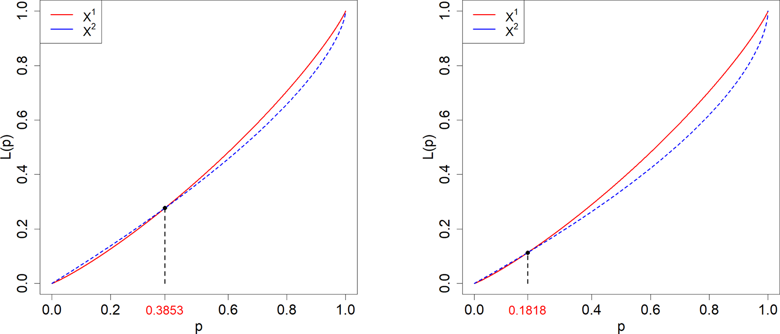


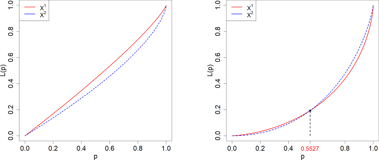


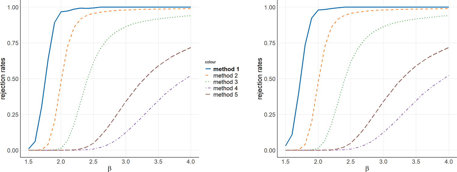


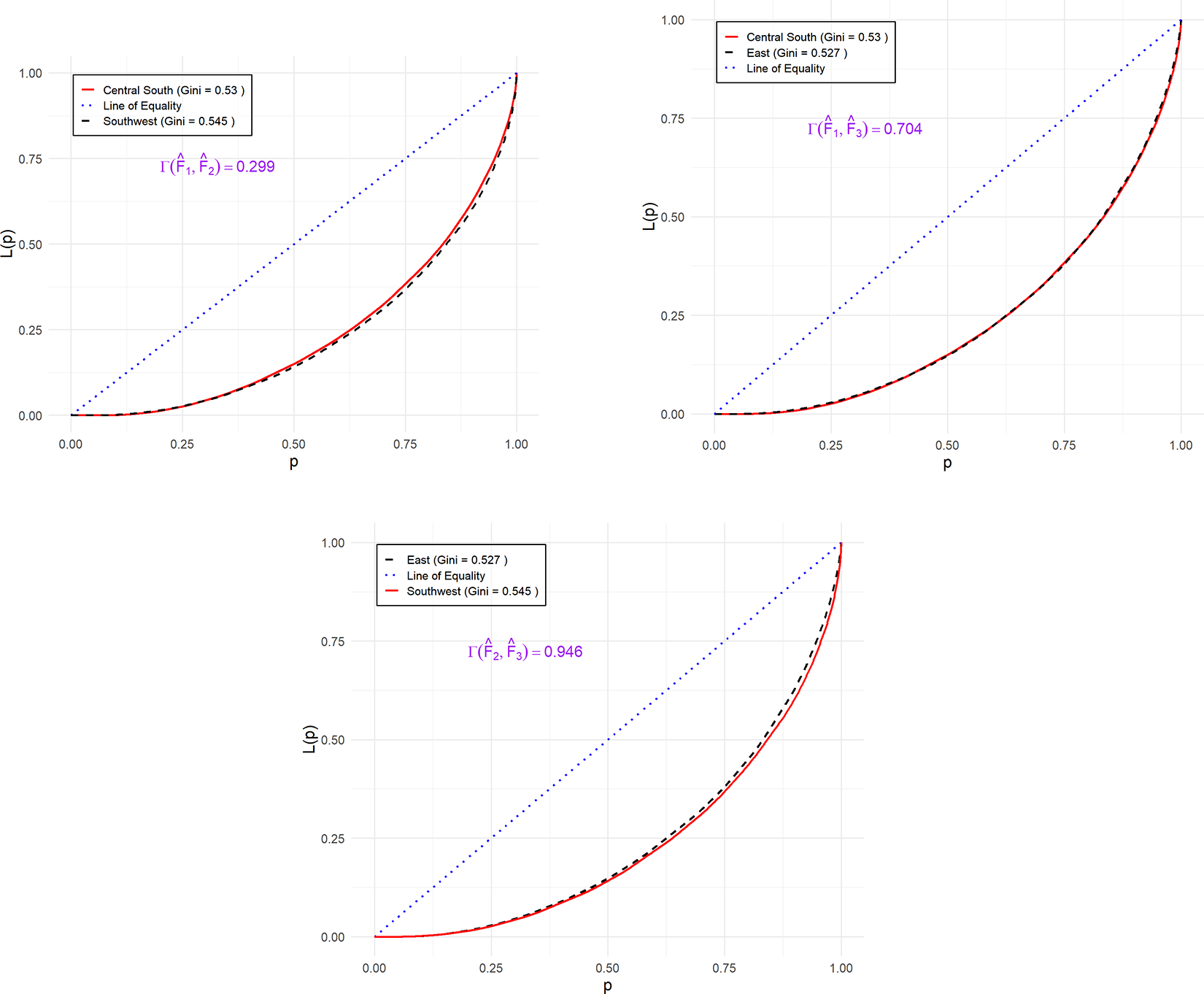


 Open access