


1. Introduction
Fluid-structure interaction (FSI) phenomenon is ubiquitous in natural and engineering systems, in which a movable or deformable structure and an internal or surrounding fluid are coupled to influence the behaviour of each other (Dowell & Hall Reference Dowell and Hall2001; Griffith & Patankar Reference Griffith and Patankar2020). The FSI problems may be further categorized into two subsets, i.e. fluid-rigid structure interaction and fluid-flexible structure interaction (Hua, Zhu & Lu Reference Hua, Zhu and Lu2014). The typical examples for the former scenario includes flow past a bluff body, e.g. cylinder (Prasanth & Mittal Reference Prasanth and Mittal2008), flat plate (Yang & Strganac Reference Yang and Strganac2013), sphere (Govardhan & Williamson Reference Govardhan and Williamson2005; Rajamuni, Thompson & Hourigan Reference Rajamuni, Thompson and Hourigan2018) and other non-streamlined bodies (Derakhshandeh & Alam Reference Derakhshandeh and Alam2019), with the vortex-induced vibration (VIV) induced on bodies interacting with an external fluid flow (Williamson & Govardhan Reference Williamson and Govardhan2004; Choi, Jeon & Kim Reference Choi, Jeon and Kim2008; Raissi et al. Reference Raissi, Wang, Triantafyllou and Karniadakis2019). The systems involving fluid-flexible structure interaction are also commonplace, e.g. swimming fish (Liu et al. Reference Liu, Ren, Dong, Akanyeti, Liao and Lauder2017), flying birds or insects (Shyy et al. Reference Shyy, Kang, Chirarattananon, Ravi and Liu2016), plant reconfiguration or flapping in a flow (Leclercq & de Langre Reference Leclercq and de Langre2018) and vibrating vocal fold (Li et al. Reference Li, Chen, Chang and Luo2019). Due to its important significance for understanding the fundamental principles in nature and the extensive engineering applications, currently, FSI is a topic of great attention in the fluid mechanics community (Dowell & Hall Reference Dowell and Hall2001; Griffith & Patankar Reference Griffith and Patankar2020).
A concern for the FSI system is how to achieve the hydrodynamic advantages or performance enhancements by means of manipulation of surrounding fluid flows (Lighthill Reference Lighthill1975; Alben Reference Alben2009; Shoele & Mittal Reference Shoele and Mittal2016). One interesting example is represented by biological flight and swimming. Fish could generate favourable flow structures for locomotion by adjusting the movement or deformation of their body and appendages (Wu Reference Wu1961, Reference Wu1971; Triantafyllou, Triantafyllou & Yue Reference Triantafyllou, Triantafyllou and Yue2000; Alben & Shelley Reference Alben and Shelley2005; Li & Lu Reference Li and Lu2012). For example, previous experimental observations (Müller et al. Reference Müller, Van Den Heuvel, Stamhuis and Videler1997; Nauen & Lauder Reference Nauen and Lauder2002) and numerical studies (Li & Lu Reference Li and Lu2012; Liu et al. Reference Liu, Ren, Dong, Akanyeti, Liao and Lauder2017) have revealed that the ring-like vortical structures formed in the wake of fish swimming possess intrinsic connections with the optimization of thrust generation and power consumption. In the flight of insects, by adopting appropriate flapping kinematics, the leading-edge vortex (LEV) stays attached to and moving with the surface of the wing, which leads to the high lift in the low  $Re$ flow region (Ford & Babinsky Reference Ford and Babinsky2013; Eldredge & Jones Reference Eldredge and Jones2019).
Beside these active flow controls for the optimal propulsion, swimming and flying animals may achieve hydrodynamic advantages from the passive flexible deformation of the propulsors (tail fins and wings) due to flow-induced loads. Results from the experimental (Mazaheri & Ebrahimi Reference Mazaheri and Ebrahimi2010; Nakata et al. Reference Nakata, Liu, Tanaka, Nishihashi, Wang and Sato2011), numerical (Kang et al. Reference Kang, Aono, Cesnik and Shyy2011; Zhu, He & Zhang Reference Zhu, He and Zhang2014; Wang, Huang & Lu Reference Wang, Huang and Lu2020) and theoretical (Michelin & Smith Reference Michelin and Smith2009; Alon Tzezana & Breuer Reference Alon Tzezana and Breuer2019; Alaminos-Quesada & Fernandez-Feria Reference Alaminos-Quesada and Fernandez-Feria2020) studies have shown that the proper flexibility of the fin or wing is found to bear performance benefits, such as thrust enhancement, drag reduction, energy saving, etc. Furthermore, as a possible strategy to reduce the drag and resist breakage, the plants living in flow-dominated habitats are able to reduce their frontal area or reshape themselves in a more streamlined fashion, which is referred to as ‘reconfiguration’ (Alben, Shelley & Zhang Reference Alben, Shelley and Zhang2002; Schouveiler & Eloy Reference Schouveiler and Eloy2013; Alvarado et al. Reference Alvarado, Comtet, de Langre and Hosoi2017; Leclercq & de Langre Reference Leclercq and de Langre2018). Compared with active flow controls, the shape self-adaptation due to flow-induced reconfiguration of flexible structure does not need the intervention of the control system or the energy input, which may be an elegant and deft way to the aero/hydrodynamic performance of the FSI system.
Not surprisingly, the flow controls by the passive deformation and flapping of flexible structures in a natural system are found universally, as they have survived the tests of evolution over millions of years and reached a high level of adaptability and effectiveness. Therefore, it is particularly worthwhile to import these novel ideas which originate from nature into technological applications, such as flow control of vortex shedding behind bluff bodies. The bluff body flow control is not only encountered in numerous natural scenarios (Triantafyllou et al. Reference Triantafyllou, Triantafyllou and Yue2000; Alvarado et al. Reference Alvarado, Comtet, de Langre and Hosoi2017; Leclercq & de Langre Reference Leclercq and de Langre2018), but also of practical interest to many fields of engineering (Choi et al. Reference Choi, Jeon and Kim2008; Dong, Triantafyllou & Karniadakis Reference Dong, Triantafyllou and Karniadakis2008; Fan et al. Reference Fan, Yang, Wang, Triantafyllou and Karniadakis2020). When the fluid flows around the bluff body, the boundary layer is likely to separate into Kármán vortices alternately shedding in the wake, which would cause the increase in differential pressure resistance (form drag). The more severe the separation at the hind side, the greater the form drag. Meanwhile, the asymmetric vortex shedding would induce large unsteady side forces that, in turn, may lead to structural vibrations if the body is flexibly mounted. Therefore, for reducing drag and suppressing VIV, controls of vortex shedding characteristics of flow over a bluff body have attracted significant attention in the past (Zhao Reference Zhao2021). Many flow control techniques have been proposed in (i) passive form and (ii) active form. The first approach includes the splitter plate (Anderson & Szewczyk Reference Anderson and Szewczyk1997; Gilliéron & Kourta Reference Gilliéron and Kourta2010), segmented trailing edges (Deshpande & Sharma Reference Deshpande and Sharma2012), dimples and grooves (Bearman & Harvey Reference Bearman and Harvey1993), etc. In these methods, global changes in the surface shape may be required for practical situations. However, it seems hard to implement under some circumstances. In the latter approach, such as blowing and suction (Schatzman et al. Reference Schatzman, Wilson, Arad, Seifert and Shtendel2014), synthetic jets (Glezer & Amitay Reference Glezer and Amitay2002), rotary oscillations (Palkin et al. Reference Palkin, Hadžiabdić, Mullyadzhanov and Hanjalić2018), the intervention of a complex control system or/and the energy input are necessary, limiting the applicability of this approach.
As a passive flow control technique, installing splitter plates behind a bluff body has been investigated by numerous experiments and simulations in the past (Anderson & Szewczyk Reference Anderson and Szewczyk1997; Gilliéron & Kourta Reference Gilliéron and Kourta2010; Wu et al. Reference Wu, Qiu, Shu and Zhao2014; Sunil, Kumar & Poddar Reference Sunil, Kumar and Poddar2022). A splitter plate, attached downstream, inhibits the interaction between the separating shear layers, thereby delaying vortex shedding and resulting in a weaker Kármán vortex street in the wake (Sunil et al. Reference Sunil, Kumar and Poddar2022). This reduces the fluctuating lift and drag acting on the bluff body. Earlier studies were mainly limited to the rigid plates. Recently, inspired by the drag-reducing mechanism of passive flexibility in natural systems, particular attention has been devoted to the flexible splitter plate (Lācis et al. Reference Lācis, Brosse, Ingremeau, Mazzino, Lundell, Kellay and Bagheri2014; Wu et al. Reference Wu, Qiu, Shu and Zhao2014; Sunil et al. Reference Sunil, Kumar and Poddar2022). It is found that a filament, with proper flexibility and length, may bring about more performance benefits in suppressing/weakening the vortex shedding as compared with a rigid splitter plate with the same length (Wu et al. Reference Wu, Qiu, Shu and Zhao2014; Sunil et al. Reference Sunil, Kumar and Poddar2022). In addition, some studies have found that installing two or multiple flexible filaments behind a bluff body, referred to as ‘hairy coating’, can offer more drag reduction under specific conditions than a single filament (Favier et al. Reference Favier, Dauptain, Basso and Bottaro2009; Niu & Hu Reference Niu and Hu2011; Deng, Mao & Xie Reference Deng, Mao and Xie2019). Favier et al. (Reference Favier, Dauptain, Basso and Bottaro2009) and Niu & Hu (Reference Niu and Hu2011) have performed the numerical and experimental investigations, respectively, on the passive flow control by using this self-adaptive hairy coating. They have shown that a sizable drag reduction can be achieved at the optimum combination of the considered parameters, e.g. hair length, rigidity, and density. The primary mechanism for drag reduction is the bending, adhesion and reinforcement of hairs trailing the bluff body, which reduces wake width and traps ‘dead water’ (Niu & Hu Reference Niu and Hu2011).
More recently, Gao et al. (Reference Gao, Pan, Wang and Tian2020) have proposed a nature-inspired passive control of the bluff body flow for drag reduction. In their experimental study, a trailing closed filament, with a negligible weight and small bending modulus, was ‘hung’ on both edges of the rigid flat plate placed normal to the oncoming flow. The experiment suggests that by adopting such a ‘flexible coating’, a significant drag reduction of approximately 10.0 % is expected under specific conditions. Compared with the existing flow control devices, this device is easy to install and disassemble. Besides, it is supposed to have good adaptability for a wide range of flows, benefiting from its nature of shape self-adaptation.
On the other hand, the study of a rigid-flexible coupling system raises a new kind of FSI problem, in which the closed flexible structure is coupled with not only an external fluid but also an internal fluid to influence the behaviour of each other. This complex interaction may give rise to a rich variety of physical phenomena which are dictated by complex mechanisms. These extended FSI systems are common in a living body in which some fluid volume is inside the thin skins of organisms, and were treated as a flexible ring filled with fluid in a surrounding fluid flow (Jung et al. Reference Jung, Mareck, Shelley and Zhang2006; Shoele & Zhu Reference Shoele and Zhu2010; Kim et al. Reference Kim, Huang, Shin and Sung2012). However, to our knowledge, still very few studies have focused on the dynamics of this coupling system.
At present, the dynamics of the rigid-flexible coupling system remain unclear. Moreover, the in-depth understanding of the corresponding flow control mechanism for drag reduction is still lacking. Inspired by Gao et al. (Reference Gao, Pan, Wang and Tian2020), we perform numerical simulations of viscous flow past a rigid flat plate with a trailing closed flexible filament. In comparison with experimental study, numerical simulations have an advantage in the aspect of quantitative analysis, which is particularly critical for exploring relevant mechanisms underlying the complex behaviour of a system. In this paper, the influence of Reynolds number ( $Re$) and length ratio of the filament and flat plate ( $Lr$) on the flow patterns and dynamics of the rigid-flexible coupling system have been systematically investigated. The drag reduction and the underlying mechanisms have been examined and revealed as well.
The rest of the present paper is organized as follows. The computational model, including physical problem and mathematical formulation, numerical method and validation, is described in § 2. The result and discussion regarding dynamic states of the rigid-flexible coupling system, drag and the flow characteristics, and drag estimate are given from a comprehensive numerical investigation in § 3. Finally, the concluding remarks are addressed in § 4.
2. Computational model
2.1. Physical problem and mathematical formulation
The rigid-flexible coupling system considered in the present study is shown in figure 1( $a$). The rigid flat plate with a trailing closed flexible filament are immersed in a two-dimensional uniform flow with oncoming velocity $U$. The rigid flat plate is fixed and placed normal to the oncoming flow. The two edges of the flexible filament are attached to the edges of the flat plate with simply support boundary conditions. The other parts of the filament can move freely and deform passively due to the flow-structure interactions. The geometry of this system is described by using a dimensionless parameter $Lr=L/D$, where $L$ and $D$ are the length of the flexible filament and flat plate, respectively. It is noted that $Lr=1$ corresponds to the situation without the trailing filament.
Schematic diagram for the rigid-flexible coupling system in a two-dimensional uniform flow ( $a$). The rigid flat plate with length $D$ is fixed and placed normal to the flow with oncoming velocity $U$. The flexible filament, severed as a deformable afterbody, is simply supported on its both edges and attached to the two edges of the flat plate. The geometry of this system is described by using a dimensionless parameter $Lr=L/D$, where $L$ is the length of the filament. Note that $Lr=1$ corresponds to the situation without the trailing filament. The initial shapes of the filament for the situations with $Lr<{\rm \pi} /2$ and $Lr \geq {\rm \pi}/2$ are illustrated in figures 1( $b$) and 1( $c$), respectively. For cases with $Lr<{\rm \pi} /2$, the initial area enclosed by the flat plate and filament is set initially to a circular segment with $Lr=\theta /{\sin }\theta$, where $\theta$ is the semi-central angle subtending the arc. While for cases with $Lr \geq {\rm \pi}/2$, the initial area is set initially to a combination of rectangle and semicircle. According to this definition, the $D^2$-normalized initial enclosed area $\varOmega _0$ can be calculated by (2.5).

In this system, the fluid flow is governed by the incompressible Navier–Stokes equations,
 $$\begin{gather} \frac{\partial \boldsymbol{v}}{\partial t}+\boldsymbol{v}\boldsymbol{\cdot}\boldsymbol{\nabla}\boldsymbol{v}={-}\frac{1}{\rho}\boldsymbol{\nabla} p+\frac{\mu}{\rho}\nabla^2\boldsymbol{v}+\boldsymbol{f}_b, \end{gather}$$
 $$\begin{gather}\boldsymbol{\nabla}\boldsymbol{\cdot}\boldsymbol{v}=0, \end{gather}$$
where  $\boldsymbol {v}=(u,v)$ is the velocity, $p$ the pressure, $\rho$ the density of the fluid, $\mu$ the dynamic viscosity and $\boldsymbol {f}_b$ the body force term. A uniform velocity $U$ is set at the inlet boundary and the side boundaries of the fluid computational domain. A Neumann boundary condition is specified at the outlet boundary.
The deformation and motion of flexible filament are described by the structural equation (Doyle Reference Doyle2001; Connell & Yue Reference Connell and Yue2007; Ye et al. Reference Ye, Wei, Huang and Lu2017),
 \begin{equation} \rho_s h\frac{\partial^2 \boldsymbol{X}}{\partial t^2} = \frac{\partial}{\partial s}\left[ Eh \left( 1 - \left| \frac{\partial \boldsymbol{X}}{\partial s} \right|^{{-}1} \right) \frac{\partial \boldsymbol{X}}{\partial s} - \frac{\partial}{\partial s} \left.\left( EI (\kappa - \kappa_0) \frac{\partial^2\boldsymbol{X}}{\partial^2 s} \right/ \left| \frac{\partial^2 \boldsymbol{X}}{\partial^2 s} \right| \right) \right] + \boldsymbol{F}_s, \end{equation}
where  $s$ is the Lagrangian coordinate along the plate, $h$ is the structure thickness, $\boldsymbol {X}(s,t)=(X(s,t),Y(s,t))$ is the position vector of the plates, $\boldsymbol {F}_s$ is the Lagrangian force exerted on the plates by the surrounding fluid and $\rho _s$ is the structural density; $Eh$ and $EI$ are the structural stretching and bending rigidity, respectively; $\kappa =| {\partial ^2 \boldsymbol {X}}/{\partial ^2 s} |$ is the local curvature of the filament with $\kappa _0$ its initial reference value. It is noted that the filament is set to be in an initial stressless reference state, according to (2.3). Moreover, the simple support boundary conditions applied at the edges of the filament are respectively given by
 \begin{equation} \boldsymbol X=({\pm 0.5},0),\quad \frac{\partial^2 \boldsymbol{X}}{\partial^2 s}=(0,0). \end{equation}
The filament is initially placed at rest in the fluid. The initial shapes of filament for the situations with  $Lr<{\rm \pi} /2$ and $Lr \geq {\rm \pi}/2$ are illustrated in figures 1( $b$) and ( $c$), respectively. For cases with $Lr<{\rm \pi} /2$, the enclosed area by the flat plate and filament is set initially to a circular segment; while for cases with $Lr<{\rm \pi} /2$, the enclosed area is set initially to a combination of rectangle and semicircle. According to this definition, the relationship between $D^2$-normalized initial area ( $\varOmega _0$) and length ratio ( $Lr$) can be given as
 \begin{equation} \varOmega_0= \begin{cases} \frac{1}{4}(\theta/{\sin^2}\theta - {\cot}\theta), & \text{if}\ Lr<\frac{1}{2}{\rm \pi} , \\ \frac{1}{2}Lr-\frac{1}{8}{\rm \pi} , & \text{if}\ Lr \ge \frac{1}{2}{\rm \pi} ,\\ \end{cases}\end{equation}
where  $Lr=\theta /{\sin }\theta$, and $\theta$ is the semi-central angle subtending the arc. In the present simulations the volume leakage is negligible which is consistent with the experiment of Gao et al. (Reference Gao, Pan, Wang and Tian2020). Thus, the enclosed area $\varOmega (t) \approx \varOmega _0$, which merely depends on $Lr$.
$Lr$.
The characteristic quantities  $\rho$, $D$ and $U$ are chosen to normalize the above equations. Thus, the following dimensionless governing parameters are introduced: the Reynolds number $Re=\rho UD/\mu$, the stretching stiffness $S=Eh/\rho U^{2} D$, the bending stiffness $K=EI/\rho U^{2} D^{3}$, the mass ratio of the plates and the fluid $M=\rho _s h/\rho D$, the length ratio of the flexible filament and the rigid plate $Lr=L/D$.
2.2. Numerical method
The governing equations of the fluid-plate problem are solved numerically by an immersed boundary-lattice Boltzmann method for the fluid motion and a finite element method for the deformation of the flexible filament. The lattice Boltzmann equation with the body force model (Guo, Zheng & Shi Reference Guo, Zheng and Shi2002) is employed in present simulations, i.e.
 \begin{equation} f_i(\boldsymbol{x}+\boldsymbol{e}_i{\rm \Delta} t, t+{\rm \Delta} t) -f_i(\boldsymbol{x},t) ={-}\frac{1}{\tau}[f_i(\boldsymbol{x},t)-f_i^{eq}(\boldsymbol{x},t)] + {\rm \Delta} t F_i, \end{equation}
where  $f_i(\boldsymbol {x},t)$ is the distribution function for particles with $\boldsymbol {e}_i$ at position $\boldsymbol {x}$ and time $t$. The D2Q9 velocity model is applied here. Here ${\rm \Delta} x$ and ${\rm \Delta} t$ are the grid spacing and time step, respectively; $\tau$ is relaxation time associated with fluid viscosity ( $\nu$), i.e. $\tau ={\nu }/{c_s^2{\rm \Delta} t} + 0.5$, where $c_s=({\rm \Delta} x/{\rm \Delta} t)/\sqrt {3}$ is the lattice sound speed. The equilibrium distribution function $f_i^{eq}(\boldsymbol {x},t)$ and the force term $F_i$ are defined as (Guo et al. Reference Guo, Zheng and Shi2002)
 $$\begin{gather} f_i^{eq}=\omega_i\rho\left[1+\frac{\boldsymbol{e}_i \boldsymbol{\cdot}\boldsymbol{v}}{c_s^2}+\frac{\boldsymbol{v}\boldsymbol{v} :(\boldsymbol{e}_i\boldsymbol{e}_i-c_s^2{\boldsymbol{\mathsf{I}}})}{2c_s^4}\right], \end{gather}$$
 $$\begin{gather}F_i=\left(1-\frac{1}{2\tau}\right)\omega_i\left[\frac{\boldsymbol{e}_i -\boldsymbol{v}}{c_s^2}+\frac{\boldsymbol{e}_i\boldsymbol{\cdot}\boldsymbol{v}}{c_s^4} \boldsymbol{e}_i\right]\boldsymbol{\cdot}\boldsymbol{f}_b, \end{gather}$$
where  $\omega _i$ is the weighting factor depending on the lattice model ( $\omega _0=4/9$, $\omega _1=\omega _2=\omega _3=\omega _4=1/9$, $\omega _5=\omega _6=\omega _7=\omega _8=1/36$), and ${\boldsymbol{\mathsf{I}}}$ is the unit tensor. The density $\rho$ and velocity $v$ can be calculated by
 \begin{equation} \rho = \sum_i f_i, \quad \rho \boldsymbol{v} = \sum_i \boldsymbol{e}_i f_i +\frac{1}{2}\boldsymbol{f}_b {\rm \Delta} t. \end{equation}
 The immersed boundary method employed in this study has been extensively used to simulate the FSI problems (Peskin Reference Peskin2002; Mittal & Iaccarino Reference Mittal and Iaccarino2005). The Lagrangian force between the fluid and structure  $\boldsymbol {F}_{s}$ can be calculated by the penalty scheme (Goldstein, Handler & Sirovich Reference Goldstein, Handler and Sirovich1993)
 \begin{equation} \boldsymbol{F}_{s}= \alpha\int^t_0[\boldsymbol{V}_f(s,t^\prime)- \boldsymbol{V}_s(s,t^\prime)]\, \mathrm{d}t^\prime +\beta[\boldsymbol{V}_f(s,t)-\boldsymbol{V}_s(s,t)], \end{equation}
where  $\alpha$ and $\beta$ are negative large penalty parameters which are selected based on the previous studies (Hua, Zhu & Lu Reference Hua, Zhu and Lu2013; Ye et al. Reference Ye, Wei, Huang and Lu2017; Peng, Huang & Lu Reference Peng, Huang and Lu2018a,Reference Peng, Huang and Luc), $\boldsymbol {V}_s=\partial \boldsymbol {X}/\partial t$ is the velocity of Lagrangian material point of the filament, and $\boldsymbol {V}_f$ is the fluid velocity at the position $\boldsymbol {X}$ obtained by interpolation
 \begin{equation} \boldsymbol{V}_f(s,t)= \int\boldsymbol{v}(\boldsymbol{x},t)\delta(\boldsymbol{x}- \boldsymbol{X}(s,t))\, {\rm d}\kern0.7pt \boldsymbol{x}. \end{equation}
 The body force term  $\boldsymbol {f}_b$ in (2.1) represents an interaction force between the fluid and the immersed boundary to enforce the no-slip velocity boundary condition. The Lagrangian force is spread to the nearby Eulerian grids by using the expression
 \begin{equation} \boldsymbol{f}_b(\boldsymbol{x},t)={-}\int\boldsymbol{F}_{s}(s,t) \delta(\boldsymbol{x}-\boldsymbol{X}(s,t))\, {\rm d}s, \end{equation}
where  $\delta (\boldsymbol {x}-\boldsymbol {X})$ is the Dirac delta function. Note that in the simulations, $\boldsymbol {f}_b$ is distributed over several Eulerian grids in width by using a smoothed delta function interpolation. Thus, the leakage of internal fluid area enclosed by the flat plate and filament may arise, due to the use of the smoothed approximation to the Dirac delta function (Kim et al. Reference Kim, Huang, Shin and Sung2012; Ye et al. Reference Ye, Wei, Huang and Lu2017).
Here we adopt a penalty forcing scheme proposed by Kim et al. (Reference Kim, Huang, Shin and Sung2012) to diminish the area leakage effect. In the scheme, the fluid compressibility  $\beta$ is defined as
 \begin{equation} \beta={-}\frac{1}{\varOmega}\frac{\partial \varOmega}{\partial p}, \end{equation}
where  $\varOmega$ is the fluid area enclosed by the plate and filament and $p$ denotes the pressure. Integrating above the differential relation between $\varOmega$ and $p$, and using Taylor's expansion, the pressure difference between the interior and exterior of the enclosed area can be approximated by
 \begin{equation} {\rm \Delta} p = \frac{1}{\beta} \left( 1- \frac{\varOmega}{\varOmega_0} \right) + \frac{1}{\beta} \int_0^t \left( 1- \frac{\varOmega}{\varOmega_0} \right) \,{\rm d} t', \end{equation}
where  $\varOmega _0$ denotes the initial interior area and the last term of the equation represents historical effects. Thus, the penalty force for area conservation is calculated by using the pressure difference ${\rm \Delta} p$ as
 \begin{equation} \boldsymbol{F}_{\varOmega}={\rm \Delta} p \boldsymbol{e}_{n}, \end{equation}
where  $\boldsymbol {e}_{n}$ represents the local normal unit in the direction from the interior to the exterior of the enclosed area. This force is also added to the structure motion equation (2.3) as an external force term.
Equation (2.3) is discretized by a nonlinear finite element method with a co-rotational scheme. A detailed description of the method can be found in Doyle (Reference Doyle2001). The motion of the filament in the present study is regarded as a large-displacement and small-strain deformation problem. By using the co-rotational scheme, the original problem with the geometrical nonlinearities in global coordinates splits into two parts, i.e. the rigid body motion and pure deformation in local coordinates, which are resolved by the coordinate transformation and linear theory, respectively. A detailed description of the above numerical method can be found in our previous papers (Hua et al. Reference Hua, Zhu and Lu2013; Ye et al. Reference Ye, Wei, Huang and Lu2017; Peng et al. Reference Peng, Huang and Lu2018a,Reference Peng, Huang and Luc; Peng, Huang & Lu Reference Peng, Huang and Lu2018b).
2.3. Validation
Based on our convergence studies with different computational domains, the computational domain for fluid flow is chosen as  $20D \times 50D$ in the $x$ and $y$ directions. The domain is large enough so that the blocking effects of the boundaries are not significant. In the $x$ and $y$ directions the mesh is uniform with spacing ${\rm \Delta} x={\rm \Delta} y=D/100$. The filament is discretized with a mesh size of ${\rm \Delta} s = D/100$. The time step is ${\rm \Delta} t=T/4000$ for the simulations of fluid flow and filament motion, with $T=D/U$.
Figure 2( $a$) shows the time histories of the changes in area with and without the penalty forcing strategy for the case with $Re=100$, $Lr=2.5$, $K=0.001$, $S=1000$ and $M=0.1$. It is seen that the maximum area leakage is $\sim 0.5\,\%$ and $\sim 12\,\%$ for the cases with and without the penalty force, respectively. The results indicate when the penalty forcing strategy is adopted, the area conservation is improved significantly and satisfied for the present study.
Validations of the present numerical method. ( $a$) The area enclosed by the flat plate and deformable filament, $\varOmega /\varOmega _0$, as a function of time for cases with and without penalty force, respectively. In these cases, $Re=100$, $Lr=2.5$, $K=0.001$, $S=1000$ and $M=0.1$. ( $b$) The variations of the mean drag coefficient as a function of $Lr$ for the cases with $Re=100$ and $\beta =5, 10, 50$. ( $c$) The time variations of $F_y$ for the cases with $Lr=2$, $Re=100$ under different lattice spacings ( ${\rm \Delta} x=D/200$, $D/100$ and $D/50$) and time steps ( ${\rm \Delta} t=T/8000$, $T/4000$ and $T/2000$). ( $d$) The variations of the mean drag coefficient as a function of $S$ for the cases of a flapping ring in a uniform flow. The present results are provided to compare with the previous results (Kim et al. Reference Kim, Huang, Shin and Sung2012). Here, $K = 0.01$, $Re= 100$ and $S=6\unicode{x2013}70$.

To examine the effect of  $\beta$ on the results of simulations, figure 2( $b$) shows the variations of the mean drag coefficient as a function of $Lr$ for the cases with $Re=100$ and varying $\beta$, i.e. $\beta =5, 10$ and 50. It is found that the choice of $\beta$ does not affect the overall drag of the coupling system for all the cases with $Lr\in (1,10]$. Whereas, it should be noted that a very small value of $\beta$ may cause numerical instability, while a very large value of $\beta$ may not guarantee volume conservation. In our simulations, $\beta =10$, which can ensure the volume conservation and numerical stability at the same time.
Also, the grid spacing and time step independence studies are performed. Figure 2( $c$) shows the time-dependent $F_y$ of the afterbody calculated under the different lattice spacings and time steps for the typical case with $Lr=2$, $Re=100$. It is confirmed that ${\rm \Delta} x=D/100$ and ${\rm \Delta} t=T/4000$ are sufficient to achieve accurate results in the present simulations with $Re=100$. Further verification shows that ${\rm \Delta} x=D/100$ and ${\rm \Delta} t=T/4000$ are also sufficient to accurately simulate the flows at higher $Re$, e.g. $Re=800$ (not shown in figure 2 $c$). Hence, in all of our simulations, ${\rm \Delta} x=D/100$ and ${\rm \Delta} t=T/4000$ were adopted.
To further validate the present numerical method, we simulate a flexible ring flapping in a uniform flow. Figure 2( $d$) shows the mean drag coefficients of the ring as functions of $S$ for $K=0.01$ and $Re=100$. It is seen that the present results agree well with those of Kim et al. (Reference Kim, Huang, Shin and Sung2012).
In addition, the numerical strategy used in this study has been validated and successfully applied to a wide range of flows, such as the dynamics of fluid flow over flexible filaments (Tian et al. Reference Tian, Luo, Zhu and Lu2010) or loops (Ye et al. Reference Ye, Wei, Huang and Lu2017), and self-propulsion of flapping flexible plates (Hua et al. Reference Hua, Zhu and Lu2013; Peng et al. Reference Peng, Huang and Lu2018a,Reference Peng, Huang and Luc).
3. Results and discussion
In the study, the effects of the length ratio ( $1\le Lr \le 10$) and Reynolds number ( $10\le Re\le 800$) are investigated. It is noted that $Lr=1$ corresponds to the situation without the trailing filament. In all our simulations, the mass ratio ( $M=0.1)$, bending stiffness ( $K=0.001)$ and stretching stiffness ( $S=1000)$ are fixed. The mass ratio is fixed at $M=0.1$, which matches the case of a flexible afterbody in the wind tunnel ( $M \sim O(10^{-1}\unicode{x2013}10^{0}$)). A large value of the stretching stiffness S is chosen such that the stretching deformation of the filament can be neglected. We chose a very small bending stiffness $K$ so that the filament is fully compliant with the surrounding flow, which is consistent with the previous experiments (Gao et al. Reference Gao, Pan, Wang and Tian2020).
3.1. Dynamic states of the rigid-flexible coupling system
In this section we present the dynamic states of the rigid-flexible coupling system in a flow. Based on a variety of simulations for a wide range of parameters considered here, we have identified five typical modes of dynamic behaviours in terms of the filament motion and flow pattern, i.e. static deformation (SD) mode, micro-vibration (MV) mode, multi-frequency flapping (MFF) mode, periodic flapping (PF) mode, and chaotic flapping (CF) mode, respectively.
Figure 3( $a$) shows the instantaneous vorticity contour and shape deformation of the filament for the case with $Re=10, Lr=2.25$, corresponding to the SD mode. Animations are also given in supplementary movie 1. It is seen that for the SD mode, the filament adapts to the streamlines of the surrounding flow and undergoes a static deformation with the fluid loading. The steady wake downstream of the plate is formed because of the low $Re$. Specifically, the shear layers with opposite vorticity formed at the edges of the plate, attached to the reshaped afterbody and then dissipated downstream (see figure 3 $a$). In addition, the snapshot of the reshaped filament for other cases with $Re=10$ and $Lr=1.1, 1.5, 4, 6, 8, 10$ are also plotted with solid green lines in figure 3( $f$). It is shown that for the SD mode, the filament appears stationary and has reflectional symmetry about its midline, behaving like a rigid body. As $Lr$ increases, the filament sequentially appears as ‘plate-like’ (e.g. $Lr=1.1$), ‘cylinder-like’ (e.g. $Lr=1.5$) and ‘slender’ (e.g. $Lr=10$) shapes, which is consistent with experimental observations (Gao et al. Reference Gao, Pan, Wang and Tian2020). It is noted that for the cases with large $Lr$, the rear part of the filament is squeezed by the surrounding fluid, yielding a rounded tip at the end of the afterbody. Figure 3( $b$) shows the instantaneous vorticity contour and shape deformation of the filament for the case with $Re=100, Lr=1.3$, corresponding to the MV mode. A video showing the vortex shedding and filament vibration is also included in supplementary movie 2. As we can see, the shear layers begin to separate at the edges of the flat plate and then form a pair of alternately shedding vortices, i.e. Kármán vortices. The figure also illustrates the development and spatial organization of the Kármán vortices in the far wake. It is seen that the alternate vortices convect downstream parallel to the centreline as two rows of vortices having opposite rotation. A snapshot of the deformation configurations of the filament is shown in figure 3( $g$). For the MV mode, the flexible filament experiences a particularly small vibration, along with the alternate shedding of the Kármán vortices. To further describe the dynamics of the filament, figure 4( $a$) shows the time variation of the lift coefficient ( $C_l$) for the overall system and transverse position of the filament midpoint ( $x_m$) for the case with $Re=100, Lr=1.3$. Here the lift coefficient is defined as $C_l={ \langle F_x \rangle }/{\frac {1}{2}\rho U^2D}$, where $\langle q \rangle := ({1}/({t_1-t_0})) \int _{t_0}^{t_1} q(t)\cdot \, {\rm d}t$ and $q(t)$ is an integrable physical quantity. In the computations, $t_1-t_0$ is chosen as 10 times $1/f_1$, where $f_1$ is the dominant frequency of the integrand. As shown in figure 4( $a$),
$a$),  $C_l$ changes with time periodically around its averaged value zero. It is also seen that the filament vibration amplitude in terms of the peak-to-peak value of $x_m$ is less than $0.04D$ (see inset within figure 4 $a$). According to the power spectrum density (PSD) of $C_l$ (see figure 4 $e$), an isolated frequency ( $f_1=0.178$) of lift change, which is equal to that of the vortex shedding and the filament micro-vibration, is observed. Note that compared with the MV mode, the lift for the SD mode case is time invariant, i.e. $C_l=0$, thus, the time variation and PSD of $C_l$ for the SD mode are not given in figure 4.
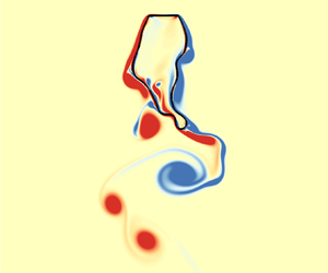
Behaviours of the flow patterns and deformations of filament shapes: ( $a$–
$a$– $e$) the instantaneous vorticity contours, and ( $f$–
$f$– $j$) the envelops (solid black lines) of the flexible filaments for five distinct modes with $Re=10$, $Lr=2.25$ (a, f), $Re=100$, $Lr=1.3$ (b,g), $Lr=2.25$ (c,h), $Lr=6$ (d,i) and $Re=800$, $Lr=9$ (e, j), corresponding to the static deformation (SD), micro-vibration (MV), multi-frequency flapping (MFF), periodic flapping (PF) and chaotic flapping (CF) modes, respectively. Animated visualisations of the dynamic states for these modes have also been provided in supplementary movies available at https://doi.org/10.1017/jfm.2022.466. For the SD mode, the snapshot of the filament deformation shapes for other cases with $Re=10$ and $Lr=1.1, 1.5, 4, 6, 8, 10$ are also plotted with solid green lines in figure 3( $f$).
$f$).

Time variations of the lift coefficient  $C_{l}$ (solid line) of the overall system and the transverse position $x_m$ (dashed line) of the midpoint of filament ( $a$–
$a$– $d$), and power spectrum density (PSD) of $C_{l}(t)$ ( $e$–
$e$– $h$) for cases with $Re=100$, $Lr=1.3$ (a,e), $Lr=2.25$ (b, f), $Lr=6$ (c,g) and $Re=800$, $Lr=9$ (d, h), corresponding to the MV, MFF, PF and CF modes, respectively. Inset: enlargement of the variation of $x_m$ versus time for the MV mode with $Re=100$, $Lr=1.3$ ( $a$1).

The behaviours of the flow pattern and the filament deformation for the case with  $Re=100$ and $Lr=2.25$, corresponding to the MFF mode, are shown in figures 3(c,h), and animated in supplementary movie 3. In this case, the Kármán vortex street is also found in the wake of the coupled system (see figure 3 $c$). It is noted that the distance between the two rows of vortices having opposite rotation becomes smaller, compared with that for the MV mode cases. Moreover, the filament experiences a flapping motion with a larger amplitude with the pick-to-pick value of $x_m \approx 0.34D$, as shown in figures 3( $h$) and 4( $b$). The curve of $C_l (t)$ in figure 4( $b$) shows a distinct pick (or valley) near the maximum (or minimum) value of $x_m$, indicating the in-phase relation between the variations of $C_l$ and $x_m$. As shown in figure 4( $f$), the PSD of $C_l$ suggests multiple discrete frequencies for the filament flapping, e.g. $f_1=0.155$, $f_2=0.472$, $f_3=0.789$, etc., whereas the first frequency $f_1$, i.e. vortex shedding frequency, is dominant.
As  $Lr$ becomes larger, the dynamic state of the system may switch from the MFF mode to PF mode. Here we use the case with $Re=100$ and $Lr=6$ as an example for the PF mode, as shown in figure 3(d,i) and supplementary movie 4. It is seen that for the PF mode, the filament flaps periodically; meanwhile, the separated shear layers become unstable, resulting in periodic alternate shedding of vortices. Different from the multiple discrete frequencies for the filament flapping in the MFF mode, an isolated frequency for the PF mode cases is found, e.g. $f_1=0.155$ for $Lr=6$ and $Re=100$, as shown in figure 4( $g$). In addition, the phase difference ${\rm \Delta} \varphi$ between the maximum $C_l$ and the maximum $x_m$ is about ${\rm \pi}$, indicating the out-phase relation between time variations of $C_l$ and $x_m$ (see figure 4 $c$).
$c$).
Figures 3( $e$) and 3( $j$) show the behaviours of the flow pattern and the filament deformation for the case with $Re=800, Lr=9$, corresponding to the CF mode. A video showing the dynamics of this case is also provided in supplementary movie 5. Here, we note that even though the flexible afterbody may deform greatly and flap strongly in the CF mode, the self-contact phenomenon has not been observed during the process of the different parts of the afterbody approaching and moving away from each other. Unlike the ordered flow patterns in the MV, MFF and PF modes, the chaotic vortical structures are found in the wake of the coupled system for the CF mode case (see figure 3 $e$). The shear layers attached to the filament start to roll up at the forepart of the afterbody and then break into eddies with varying sizes irregularly shedding in the wake (see figure 3 $e$), accompanied by the chaotic flapping of the filament (see figure 3 $j$). Furthermore, the curves of $C_l(t)$ and $x_m(t)$ illustrate the dynamic disorder of the coupled system, as shown in figure 4( $d$). Moreover, figure 4( $h$) shows the PSD of $C_l$ for the case with $Re=800, Lr=9$. As one can see, figure 4( $h$) shows a broadband spectrum, indicating a non-periodic behaviour of the coupled system. Moreover, a high peak is found at $f_1=0.140$ (see figure 4 $h$), showing the dominant flapping frequency for the filament flapping and vortex shedding. In the discussion above, it is interesting to note that there is an obvious difference in the phase relation between $C_l$ and $x_m$ for the MFF and PF modes. To further illustrate this point, the variations of the phase difference ${\rm \Delta} \varphi$ between the maximum $C_l$ and the maximum $x_m$ as functions of $Lr$ for different $Re$ are shown in figure 5( $a$). It is seen that the system mode switches from the MFF mode to PF mode as $Lr$ increases, resulting in a jump of ${\rm \Delta} \varphi$, e.g. ${\rm \Delta} \varphi \approx 0$ for the MFF mode case with $Re=100$, $Lr=2$ and ${\rm \Delta} \varphi \approx {\rm \pi}$ for the PF mode case with $Re=100$, $Lr=7$. Moreover, the root-mean-square (rms) values of the transverse position of the filament midpoint, $x_{m,{rms}}$, as functions of $Lr$ for various $Re$, are shown in figure 5( $b$). It is revealed that as the increase of $Lr$,
$Lr$,  $x_{m,{rms}}$ follows obviously different variations within different mode regions. For example, when $Re> 50$, the $x_{m,{rms}}$ first increases linearly within the MV mode region ( $Lr<2$), and then experiences an enormous increase by following a logarithmic growth law until reaching its maximum value at $Lr\thickapprox 3.5$. After that, $x_{m,{rms}}$ gradually decreases and stabilizes. Therefore, one can distinguish the boundaries between the distinct modes through the curve profiles of ${\rm \Delta} \varphi$ and $x_{m,{rms}}$. Our results indicate that the occurrence of the motion states of the system depends mainly on the length ratio $Lr$ and Reynolds number $Re$. The phase diagram for the five modes in the $H\unicode{x2013}Re$ plane is shown in figure 6. Each symbol in the figure represents a case we simulated. It is seen that the SD mode occurs mainly in the low $Re$ region (say $Re=10$). As $Re$ increases, the transition from a steady to unsteady state for flow past the coupled system is found at a critical $Re \in (25, 50)$ for $1\le Lr < 4$, or $\in (10, 25)$ for $4\leq Lr \leq 10$. In the moderate $Re$ region (say $Re=100$), the MV, MFF, PF and CF modes appear in succession as $Lr$ increases from 1.1 to 10; when $Re$ is large enough (say $Re=800$), only the MV and CF modes occur.
( $a$) Phase difference between the peaks of $C_l$ and $x_m$, and ( $b$) the root-mean-square value of the transverse position of the filament midpoint, $x_{m,{rms}}$, as functions of $Lr$ for various $Re$.
$Re$.

Overview of the five typical mode regions on the  $Lr\unicode{x2013}Re$ plane, where the symbols $\diamond$, $\square$, $\circ$, $\vartriangle$ and $\triangleright$ represent the SD, MV, MFF, PF and CF modes, respectively. The drag reduction region (DRR) is marked by the grey colour. The $Lr_{c,{max}}$ (or $Lr_{c,{min}}$) trajectory along which the system experiences a local maximum (or minimum) drag is plotted by the dashed (or dash-dotted) line on the phase plane. The typical cases in figure 3 are marked by the symbols $\times$.

3.2. Drag and the flow characteristics
The drag acting on the coupled system by the surrounding fluid is further investigated to better understand the relationship between the drag variations and the mode transitions. The jump in the fluid force across the plate or filament at a certain Lagrangian point, i.e  $\boldsymbol {F}_s$, can be decomposed into two parts: one is the normal force $\boldsymbol {F}^n$ in which the pressure component dominates, the other is the tangential force $\boldsymbol {F}^{\tau }$ which comes from the viscous effects. These forces are defined as
 $$\begin{gather} \boldsymbol{F}_s=[{-}p{\boldsymbol{\mathsf{I}}}+{\boldsymbol{\mathsf{T}}}]\boldsymbol{\cdot} \boldsymbol{n}=\boldsymbol{F}^n+ \boldsymbol{F}^{\tau}=(F_x, F_y), \end{gather}$$
 $$\begin{gather}\boldsymbol{F}^{n}=(\boldsymbol{F}_s\boldsymbol{\cdot}\boldsymbol{n})\boldsymbol{\cdot} \boldsymbol{n}=(F^{n}_x,F^{n}_y), \end{gather}$$
 $$\begin{gather}\boldsymbol{F}^{\tau}= (\boldsymbol{F}_s\boldsymbol{\cdot}\boldsymbol{\tau})\boldsymbol{\cdot}\boldsymbol{\tau}= (F^{\tau}_x,F^{\tau}_y), \end{gather}$$
where  ${\boldsymbol{\mathsf{I}}}$ is the unit tensor, ${\boldsymbol{\mathsf{T}}}$ the viscous stress tensor, $\boldsymbol {\tau }$ the unit tangential vector, $\boldsymbol {n}$ the unit normal vector and $[~]$ denotes the jump in a quantity across the immersed boundary. The system experiences a fluid drag in the $y$ direction, i.e $-F_y = -(F_y^n + F_y^{\tau })$. Thus, the corresponding time-averaged drag coefficients are defined as $C_d=-\langle F_y \rangle /\frac {1}{2}\rho U^2D$, $C_d^{n}=-\langle F_y^n \rangle /\frac {1}{2}\rho U^2D$ and $C_d^{\tau }=-\langle F_y^{\tau } \rangle /\frac {1}{2}\rho U^2D$, respectively. Figure 7( $a$) shows the fluid drag curves versus $Lr$ at different $Re$ for the overall system. Here the drag is normalized by that for the bare plate scenario. It is seen that the drag curves show two distinct tendencies depending on the $Re$. For the flow at a low Reynolds number (say $Re=10$ or 25), the drag almost monotonically increases with the increase of $Lr$. For the higher Reynolds flow (e.g. cases with $Re\ge 50$), the drag first decreases from $C_d/C_{d,Lr=1}=1$ as $Lr$ increases, and reaches a local minimum at $Lr=Lr_{c,{min}}$. After that, the drag curve shows a sharp rise until the second threshold at $Lr=Lr_{c,{max}}$, where the system experiences a local maximum drag. When $Lr>Lr_{c,{max}}$, the fluid drag generally shows a slow decline as $Lr$ increases. Moreover, we denote the $Lr_{c,{min}}$ (or $Lr_{c,{max}}$) trajectory in the $Lr\unicode{x2013}Re$ plane, as shown in figure 6. It is found that the emergencies of local minimum (or maximum) drags at $L_{c,{min}} \in [1.8, 2]$ (or $L_{c,{max}} \in [3.5, 4]$) are often accompanied by the system state transitions. Furthermore, it is interesting to note that benefiting from the passive flow control by using the trailing filament as a deformable afterbody, the system may experience a counterintuitive reduction in fluid drag, corresponding to the scenarios within the grey region ( $C_d/C_{d, Lr=1}<1$) marked in figure 7( $a$). Compared with the bare plate, the system enjoys a dramatic drag reduction (up to approximately $22\,\%$) at $Lr \approx L_{c,{min}}$ for $Re\ge 50$. The considerable reductions in drag are also observed for cases with large $Lr$ and high $Re$, e.g. $Lr>5$ and $Re\geqslant 400$. As shown in figure 6, we denote the drag reduction region (DRR) in the $Lr\unicode{x2013}Re$ phase plane for the overall system. The critical value of $Re$, i.e. $Re_c$, separating the DRR and drag increase region (DIR) generally depends on $Lr$. Specifically, $Re_{c} \in (25,50)$ for $1\leq Lr\leq 2$ while $Re_{c} \in (100,200)$ for $4\leq Lr\leq 10$; $Re_c$ increases as the increase of $Lr$ for $2< Lr<4$. The DDR almost covers the region with $Re>Re_{c}$ except for the cases with $Re=800$, $Lr=1.1$ and 1.3. Compared with the experiment (Gao et al. Reference Gao, Pan, Wang and Tian2020) with a higher $Re \sim 2700\unicode{x2013}5500$, our simulations also show that the counterintuitive drag reduction due to the flow-induced reconfiguration of filament may arise in the low-moderate $Re$ ( $\sim 10\unicode{x2013}10^3$) flow region. The experimental data from Gao et al. (Reference Gao, Pan, Wang and Tian2020) with $Re=4400$ which is based on the speed of uniform inflow $U_{\infty }=1.54$ m s $^{-1}$ are plotted in figure 7( $a$). It is worth noting that, although the numerical results are not in perfect agreement with the experimental data (which to some extent is expected given the higher $Re$ flow in the soap film experiments), similar trends in drag variation have been found in the experiments and present simulations; in particular, the $Lr_{c,{min}}$ (or $Lr_{c,{max}}$) obtained from the experiment is very close to that from the simulations with $Re\ge 400$ (see figure 7 $a$). The experimental and numerical results have shown together that this kind of device, referred to as a ‘flexible coating’, may have a high level of adaptability and effectiveness for the flow control for reducing drag of the bluff body in a flow.
( $a$) Fluid drag acting on the coupled system normalized by the drag of the isolated rigid plate, i.e. $C_d/C_{d,Lr=1}$ as functions of $Lr$ for various $Re$. The drag for the system can be decomposed into two parts, i.e. the tangential one $C_d^{\tau }/C_{d,Lr=1}$ ( $b$) which comes from the viscous effects, and the normal one $C_d^{n}/C_{d,Lr=1}$ ( $c$) in which the pressure component dominates. Inset: $C_d^{n}/C_{d,Lr=1}$ for the rigid plate ( $c1$) and the flexible filament ( $c2$), respectively. For the overall system, $C_d/C_{d,Lr=1}<1$ corresponds to the drag reduction scenarios, which is located in the grey region in figure 7( $a$). Also, the experimental data (Gao et al. Reference Gao, Pan, Wang and Tian2020) with $Re=4400$, which is based on the speed of uniform inflow $U_{\infty }=1.54$ m s $^{-1}$, are plotted in figure 7( $a$).
$a$).

Further, the drag-reducing effect by using a flexible afterbody is compared with that using a rigid one for the typical cases as listed in table 1. The geometry of a rigid afterbody is represented by the time-averaged shape of a flexible one with identical  $Lr$. It is found that for the cases with $Lr= Lr_{c, {min}}$ (i.e. cases 1–4), the drag reduction can be achieved by using a flexible or rigid afterbody, whereas the ‘flexible coating’ may give rise to more benefit in drag reduction of the system, especially in the higher $Re$ region considered here, e.g. $Re=800$ (case 4 in table 1). These facts suggest that suitably adding a flexible coating to a rigid body may lead to additional reduction in drag relative to conventional flow control devices/measures, e.g. rigid splitter plates or other streamlining, in which the FSI effect is not included. Moreover, it should be noted that a flexible afterbody may also lead to a larger fluid drag of the overall system compared with a rigid one when $Lr$ is larger, e.g. case 5 in table 1.
Comparison for the drag coefficients ( $C_d$ and $C_d/C_{d, Lr=1}$) of the overall systems with the flexible and rigid afterbodies for typical cases. Here, for cases 1–4, the length ratio $Lr= Lr_{c, {min}}$, at which the maximum reduction in drag is achieved in the flexible scenarios (see figure 7 $a$). The geometry of a rigid attachment is represented by the time-averaged shape of the flexible afterbody with the identical $Lr$.
$Lr$.

Figures 7( $b$) and 7( $c$) show the contributions to the total drag from the viscous and pressure stresses for the system, i.e. $C_d^{\tau }/C_{d,Lr=1}$ and $C_d^n/C_{d,Lr=1}$, respectively. For the SD mode cases with $Re=10$, it is seen that, as $Lr$ increases, the friction contribution increases from approximately zero to 0.8, while the pressure contribution reduces from approximately 1 to 0.65. Thus, for the whole system, the form drag predominates at the small $Lr$, but is no longer the exclusively dominating force at the large $Lr$, where the skin friction drag cannot be neglected. As $Re$ increases, the friction drag is greatly reduced, e.g. $C_d^{\tau }/C_{d,Lr=1}<0.25$ for $Re \geq 100$, resulting in the form drag predominating in the total drag for high $Re$ cases. Because of this, it is seen from figures 7( $a$) and 7( $c$) that the form drag changes with a similar tendency as that of the total drag within the high $Re$ region. We further show the form drag curves at varying $Re$ for the rigid and flexible parts in inset figures 7( $c1$) and 7(c2), respectively. It is observed that when $Lr$ is close to 1, e.g. $Lr=1.1$, where the flow pattern is similar to that of the bare plate scenario, the trailing filament contributes almost the same form drag as the rigid plate, as shown in figure 7( $c$2). As $Lr$ further increases, the form drag on the filament for all $Re$ cases decreases firstly until the first threshold at $Lr_{c,{min}}$, where the form drag reduction is up to nearly $30\,\%$ in comparison with that at $Lr=1$. After $Lr > Lr_{c,{min}}$, the filament experiences the distinct form drag variations for the low $Re$ region (e.g. $Re=10$) and high $Re$ region (e.g. $Re>100$), respectively (see figure 7 $c$2), which is similar to that for the overall system as shown in figure 7( $c$). Moreover, it is noted that as $Lr$ increases, small changes in the form drag of the rigid plate are observed at most $Re$, e.g. $Re=10$ or $\geq 100$. These facts indicate that the drag reduction for the coupled system is mainly derived from the passive controls for the favourable flow over the flexible trailing filament.
To further explore the underlying mechanisms of the counterintuitive drag reduction behaviour of the coupled system, the corresponding flow characteristics are investigated in the following. Figure 8 shows the time-averaged vorticity and pressure contours around the structures, as well as the vertical component of fluid loads on their surfaces for typical cases. For the isolated plate in the flow, i.e. the case with  $Re=100$ and $Lr=1$ as shown in figures 8(a,e,i), it is clear in a time-averaged sense that a low-pressure region on the lower surface and a high-pressure region on the upper surface of the plate (figure 8 $e$), which is induced by the opposite vortex pair (figure 8 $a$) and the fluid deceleration effect, respectively, dominate nearly the overall drag of the plate (figure 8 $i$). Unlike the isolated plate case, for the case with $Re=100$ and $Lr=2$ in figure 8(b, f, j), the vortex pair is stretched downstream, and the vorticity in the shear layer is mainly distributed on both sides of the filament. This vorticity distribution induces a weakened low-pressure region directly below the filament (figure 8b, f), leading to an obvious drag reduction (figure 8 $j$). It is noted that because the flow separation occurs early due to the large reverse pressure gradient near the front outer surface of the filament (see figure 8 $f$), the contribution of viscous friction to the total drag is negligible in comparison with that of the pressure (see figure 8 $j$). For the case with $Re=100$ and $Lr=3.5$, as shown in figure 8(c,g,k), the filament achieves a more streamlined time-averaged shape by adapting itself to the surrounding fluid, which is helpful for the shear layers attaching to the surfaces (figure 8 $c$). In this case, as shown in figure 8( $k$), the fluid drags contributed by the pressure and the friction mainly distribute on the top/bottom and side surfaces of the enclosed loop, respectively; the form drag is still dominant, but the fiction drag is no longer negligible. Thus, compared with the bare plate scenario, although the form drag slightly reduces, the total drag increases due to the addition of fiction (see figure 7). For the case with $Re=10$ and $Lr=9$, as shown in figure 8(d,h,l), it is seen that unlike the cases discussed above, the filament is subjected to a considerable fiction drag and a negligible form drag, owing to its highly streamlined steady deformation. Thus, in this case, the form drag and the friction drag are almost contributed by the rigid plate and the flexible filament, respectively (see figure 8 $l$).
$l$).
Time-averaged vorticity ( $a$–
$a$– $d$) and pressure ( $e$–
$e$– $h$) contours around the coupled system, and the distribution of the $y$ component of time-averaged normal and tangential force ( $i-l$) for the typical cases with $Re=100$, $Lr=1$ (a,e,i), 2 (b, f, j), 3.5 (c,g,k) and $Re=10$, $Lr=8$ (d,h,l), respectively. The two vectors, i.e. ( $0,F_y^n$) (red colour) and ( $0,F_y^\tau$) (blue colour), are plotted along the plate and filament, illustrating the spatial distribution of the fluid drags contributed by the pressure and friction, respectively.

Figure 9 shows the unsteady behaviours for the typical cases with  $Re=100$, $Lr=1$, 2 and 3.5. For the bare plate scenario ( $Re=100$, $Lr=1$), the shear layers separate at the edges of the flat plate and form a pair of counter-rotating vortices alternately shedding in the wakes (see figure 9 $g$), which causes the periodic fluctuations in pressure on the lower surface of the plate, as we can see in the curve of $F_y(t)$ (see figure 9 $a$). From the instantaneous flow field around the plate at instant A, corresponding to the valley in the curve of $F_y(t)$ as shown in figure 9( $a$), it is clear that the maximum instantaneous drag is attributed to the low-pressure region induced by the vortex which moves just below the plate at instant A, as shown in figure 9( $d$). For the case with $Re=100$ and $Lr=2$, a similar situation is observed in the instantaneous flow field (see figure 9 $e$) at instant B when the maximum instantaneous drag is achieved, as shown in figure 9( $b$). The difference from the bare plate case is that the moving vortex is weaker and, thus, the induced low-pressure region is weakened, resulting in a smaller drag peak. For the case with $Re=100$ and $Lr=3.5$, a dramatic peak is found in the curve of $F_y(t)$ at instant C as shown in figure 9( $c$). From figure 9( $f$), we can see that at the trailing end of the afterbody, the local high and low pressure appear on the inner and outer surfaces, respectively, which is responsible for the sharp increase of the drag at instant C. It is also noted that at this moment, the left shear layer with positive vorticity is able to maintain attachment to the reshaped and moving surface (see figures 9f,i), and such attached flow will provide a considerable contribution to friction drag (figure 8 $k$).
$k$).
The unsteady behaviours of the coupled system: ( $a$–
$a$– $c$) the $y$ component of fluid force for the system, $F_y$, and the transverse position of the filament midpoint, $x_m$, as functions of time for $Re=100$, $Lr=1$ ( $a$), 2 ( $b$) and 3.5 ( $c$); ( $d$–
$d$– $f$) the instantaneous pressure contours and streamlines around the coupled system at instant A for $Re=100$, $Lr=1$ ( $d$), instant B for $Re=100$, $Lr=2$ ( $e$) and instant C for $Re=100$, $Lr=3.5$ ( $f$); ( $g$–
$g$– $i$) the instantaneous vortical structures in the far field for $Re=100$, $Lr=1$ ( $g$), 2 ( $h$) and 3.5 ( $i$). The paths of the vortex with positive (anticlockwise rotation) and negative (clockwise rotation) circulation are plotted by the solid and dashed lines, respectively. The position of the vortex core is identified by $x_c ={\int x \omega _z \,{\rm d}S}/{\int \omega _z \,{\rm d}S}$ and $y_c ={\int y \omega _z\, {\rm d}S}/{\int \omega _z \,{\rm d}S}$. ( $j$–
$j$– $l$) The time-averaged velocity deficit induced by the vortex street in the wake for $Re=100$, $Lr=1$ ( $j$), 2 ( $k$) and 3.5 ( $l$). The contours show the magnitude of the time-averaged velocity in the $y$ direction, and the velocity profiles in the far field are also illustrated by the vectors (0, $v$) at $y=-12$.

From the discussion above, the generation, movement and shedding of vortices around the coupled system play a prominent role in the dynamic characteristics, especially the fluid drag of the system. We further explore the vortex structures in the far field and their relation to changes in drags. For cases with  $Re=100, Lr=1, 2$ and 3.5, as shown in figure 9(g,h,i), the Kármán vortex streets, associated with the averaged drag force (Griffin & Ramberg Reference Griffin and Ramberg1975; Li & Lu Reference Li and Lu2012), are observed in wakes. Here, the Kármán vortex street is characterized by the distance between its two staggered rows of vortices, $w$, the streamwise separation between the adjacent vortices having opposite rotation, $h$, and the vortex circulation $\varGamma$. The position of the vortex core is defined as $x_c ={\int x \omega _z \, {\rm d}S}/{\int \omega _z \, {\rm d}S}$ and $y_c ={\int y \omega _z\, {\rm d}S}/{\int \omega _z \, {\rm d}S}$. For the system, the averaged drag force is relevant to the reverse jet flow in the vertical direction induced by the vortices. As illustrated in figure 9( $g$), according to the vortex-dipole model (Godoy-Diana et al. Reference Godoy-Diana, Marais, Aider and Wesfreid2009), the vertical component of the dipole-induced velocity is
 \begin{equation} V_y^{\varGamma}=V^{\varGamma}{\cos}\alpha= \frac{\varGamma}{2{\rm \pi} d} \times {\cos}\alpha=\frac{\varGamma w}{2{\rm \pi} (w^2+h^2)}, \end{equation}
where  ${\cos }\alpha =w/d$ and $d=\sqrt {h^2+w^2}$. For comparison of three typical cases with $Re=100$ and $Lr=1$, 2 and 3.5, the parameters of Kármán vortex streets are given in table 2. It is seen that compared with the bare plate case ( $Re=100$, $Lr=1$), the vortex street width for the drag reduction case ( $Re=100$, $Lr=2$) is significantly narrower, which results in a substantial increase of $\alpha$ and decrease of the value of cos $\alpha$. This would result in a weakened reverse jet flow with a smaller $V_y^{\varGamma }$ according to (3.4). However, for the case with $Re=100$ and $Lr=3.5$, the enhanced reverse jet flow with larger $V_y^{\varGamma }$, corresponding to the increased drag, is mainly attributed to the more increase of vortex circulation $\varGamma$, relative to the less decrease (or increase) of the value of $\cos \alpha$ (or $d$).
$d$).
Parameters of Kármán vortex streets for cases with  $Re=100$ and $Lr=1$, 2 and 3.5. Here, $\varGamma$, $w$,
$w$,  $h$ and $\alpha$ are the parameters determined based on the flow field. Here $V_y^{\varGamma }$ is calculated by using (3.4).

Further, figure 9( j–l) shows the time-averaged vertical velocity contours and velocity profiles in the wake for the three cases. As we can see, the velocity deficit (wake profile), induced by Kármán street with the reverse jet, arises in the far field for all the cases, indicating the onset of net fluid drag acting on the system. Moreover, it is seen that compared with that for the bare plate case ( $Re=100, Lr=1$), the intensity of reverse jet flow is weakened for the drag reduction case ( $Re=100, Lr=2$), but enhanced for the drag increase case ( $Re=100, Lr=3.5$), respectively. And a weakened (or enhanced) reverse jet can be considered as a prognosticator of a further drop (or increase) in drag. These findings indicate that the flexible filament coating to a rigid plate may offer favourable flow controls for the vortex dynamics in the near field and in the far field, which brings in sizable drag reduction for the overall system.
3.3. Drag estimate
In this section the form drag and the friction drag, which come from the pressure and viscous effects, respectively, are further estimated. According to the Blasius solution (Schlichting & Gersten Reference Schlichting and Gersten2016) for the flow along a very thin flat plate, the friction drag on one side of the flat plate  $\sim \rho U^2L_{f} ({UL_{f}}/{\nu })^{-1/2}$, where $U$ is free-stream velocity and $L_{f}$ is the length of the flat plate, indicating that the friction drag is proportional to $U^{3/2}$ and to $L_{f}^{1/2}$. From the discussion above, it is revealed that the friction drag mainly originates from the attached shear layer on the outer surface of the filament. Therefore, by assuming the friction drag on the filament surface follows the same scaling rule, we have $C_d^{\tau } \sim ({L_{\tau }/Re})^{1/2}$, where $L_{\tau }$ is the dimensionless characteristic length of the frictional layer scaled by $D$ and $Re =\rho UD/\mu$. Thus, the coefficient of friction drag on the filament can be estimated by
 \begin{equation} C_d^{\tau} = 2k_{\tau}\sqrt{\frac{L_{\tau}}{Re}}, \end{equation}
where  $L_{\tau }=(Lr-1)/2$ and $k_\tau$ is a dimensionless constant coefficient.
Figure 10( $a$) shows the variation of $C_d^\tau$ as $({L_{\tau }/Re})^{1/2}$. As we can see, all the data from the present simulations appear to collapse into a straight line described by (3.5) with $k_\tau \approx 1.8$, indicating that the friction drags calculated by (3.5) agree well with the numerical results. It is noted that the constant coefficient $k_{\tau }$ derived from the Blasius solution for the flat plate boundary layer is 1.328, which is smaller than $k_{\tau }=1.8$ from the numerical results. One should also note that the Blasius solution with $k_{\tau }=1.328$ is only valid in the limit of $Re>>1$, which is not the case with low-moderate $Re$ in the present simulation. In spite of this, our numerical results indicate that $(L_{\tau }/Re)^{1/2}$ may serve as a practicable metric for scaling the friction drags. On the other hand, the form drag arises from the pressure difference on the upper and bottom surfaces of the enclosed system, which is closely related to filament flapping and deformable shape. Thus, the transverse characteristic length of the afterbody is a more important factor than the streamwise length for scaling the form drag. Since the afterbody is subjected to a shape deformation or strong flapping for most cases in our simulations, the flat plate width $D$ can not serve as a good characteristic length for scaling the form drag, as shown in figure 7. Therefore, we here adopted the maximum width of the afterbody envelope $W$ as a characteristic length to renormalise the form drag, i.e. $C_{d,W}^{n}=C_{d}^{n}\times {1}/{W^*}=-\langle F_y^n \rangle /\frac {1}{2}\rho U^2 W$, where the dimensionless quantity $W^*={W}/{D}$.
Scaling laws for the friction drag ( $a$) and the form drag ( $b$) acting on the coupled system, which come from viscous effects and pressure differences, respectively. The friction drags $C_d^\tau$ and the renormalised form drag $C_{d,W}^{n}$ are plotted as functions of $({L_{\tau }}/{Re})^{1/2}$ and $Lr$, respectively. A new drag coefficient, $C_{d,W}^{n}$, is normalised using the maximum width of the afterbody envelope $W$, instead of $D$. Inset gives the variation of $C_{d}^{n}$ versus $Lr$ for $Re=10$. Results indicate that the friction drags follow the scaling law of $C_d^\tau \sim ({L_{\tau }}/{Re})^{1/2}$ for all the $Re$ numbers considered here; while the form drags follow the scaling laws of $C_{d,W}^{n} \sim Lr^{-0.60}$ for $Re\ge 25$ and $C_{d}^{n} \sim Lr^{-1.27}$ for $Re=10$, respectively. Legend is identical to that in figure 7.

Figure 10( $b$) shows the variation of $C_{d,W}^n$ versus $Lr$ for $Re \geq 25$. It is shown that the symbols with $Re \geq 25$ appear to collapse nearly into a curve described by $C_{d,W}^{n}=2.66 Lr^{-0.60}$. It is also noted that the symbols in the large- $Lr$ region (say $Lr>3$) are closer to the scaling curve than those in the small- $Lr$ region. The results in figure 10( $b$) suggest that $W$ is a reasonable characteristic length for scaling form drag in flapping regions, especially in large-amplitude flapping regions, i.e. $Lr>3$ (see figure 4 $b$). While for the static deformation region with $Re=10$, $W$ is no longer a characteristic length for the form drag. As shown in the inset in figure 10( $b$), the coefficient $C_d^n$ can be merely described by $Lr$, i.e. $C_d^n = 1.20Lr^{-1.27}+1.84$. Thus, the form drag on the system for all the $Re$ numbers considered can be estimated by
 \begin{equation} C_d^{n}= a \times \frac{W^{*n}}{Lr^b} + c, \quad \text{where } \begin{cases} a=2.66, b=0.60, c=0, n=1, & \text{if } Re \geq 25, \\ a=1.20, b=1.27, c= 1.84, n=0, & \text{if } Re= 10. \end{cases} \end{equation}
Finally, the overall drag coefficient can be estimated by
 \begin{equation} C_d^{'}=C_d^{\tau '}+C_d^{n'}=2k_{\tau}\sqrt{\frac{L_{\tau}}{Re}}+a \times \frac{W^{*n}}{Lr^b} + c. \end{equation}
It is noted that for a short afterbody, e.g.  $Lr<3$, the transverse characteristic length is no longer the only dominant metric for scaling drag, and, thus, the deviation of $C_d^n$ estimated is slightly larger, compared with that for a slender afterbody, as shown in figure 10( $b$). In order to eliminate this error, a correction factor $\gamma$ based on the drag of a bare rigid plate is introduced. Therefore, the modified drag estimate formula is expressed by
 \begin{equation} C_d^{''} = 2k_{\tau}\sqrt{\frac{L_{\tau}}{Re}} + \gamma \times \left(a\frac{W^{*n}}{Lr^b} + c\right), \end{equation}
where  $\gamma = C_{d,Lr={1}}/C_{d,Lr={1}}^{'}= C_{d,Lr={1}}/C_{d,Lr={1}}^{n'}$ for $Lr<3$, and $\gamma =1$ for $Lr\geq 3$.
Figure 11 shows the variations of  $C_d/C_{d,Lr=1}$ as a function of $Lr$ for $Re=10\unicode{x2013}800$. All the data in figure 7( $a$) are plotted again in figure 11 with the same symbols, and each curve in figure 11 denotes the estimated drag calculated using (3.8) for each $Re$, respectively. It is seen that the estimate curves, which are based on the scaling laws for friction drag and form drag, show a similar tendency to those in the simulations. Moreover, we note that a good degree of agreement between the numerical and estimate data is observed at even high- $Re$ and large- $Lr$ regimes, in which the flow is highly unsteady and the filament flaps strongly. The drag scaling laws proposed here are helpful for understanding the underlying mechanism of the drag variations and may give valuable insight into the dynamics of this type of FSI system.


4. Concluding remarks
In summary, we carried out a numerical investigation on the dynamics of fluid flow past a rigid flat plate with a trailing closed flexible filament acting as a deformable afterbody. We have found the five distinct modes of the system state according to the filament motion and flow pattern, i.e. SD, MV, MFF, PF and CF modes. It was indicated that the occurrence of the system mode depends mainly on  $Lr$ and $Re$. The phase diagram for the typical modes in the $Lr$–
$Lr$– $Re$ plane were plotted.
The drag variations show two distinct tendencies in lower and higher  $Re$ regions. For the flow at low Reynolds number, the drag almost monotonically increases with an increase of $Lr$. While for the higher Reynolds flow, all the $C_d(Lr)$ curves indicate the existence of the local minimum (or maximum) drags at $L_{c,{min}} \in [1.8, 2]$ (or $L_{c,{max}} \in [3.5, 4]$). Besides, we also noted that the $L_{c,{min}}$, or $L_{c,{max}}$, trajectory generally separates different mode regions in the $Lr\unicode{x2013}Re$ plane. In other words, as $Lr$ changes, the overall system may reach its local minimum or maximum drag, along with the emergence of state transition. Moreover, it was interesting to note that benefiting from the passive flow control by using the trailing filament as a deformable afterbody, the system may experience a counterintuitive reduction in fluid drag. Compared with the bare plate, the system enjoys a dramatic drag reduction up to approximately $22\,\%$; and the considerable reductions in drag were also observed for cases with large $Lr$ and high $Re$, e.g. $Lr>5$ and $Re \ge 400$.
The analysis of time-averaged and instantaneous flow fields shows that drag reduction is mainly attributed to favourable control for the shedding and movement of vortices around the flexible afterbody. The velocity deficit (wake profile) induced by the Kármán vortices arises in the far field, indicating the onset of net fluid drag acting on the system. To explore the relations between drag and vortical wake, the characteristics of Kármán vortex streets in the far field for typical cases are quantificationally described by using  $w$,
$w$,  $h$ and $\varGamma$. For the drag reduction case, the vortex street width ( $w$) is significantly narrower and, thus, the strength of the reverse jet is weakened.
The drag decomposition shows that the form drag predominates at the small  $Lr$ but is no longer the exclusively dominating force at large $Lr$, where the skin friction drag cannot be neglected. As $Re$ increases, the friction drag is greatly reduced, resulting in the form drag predominating in the total drag for high $Re$ cases. Finally, the overall drag is estimated based on the scaling laws for the friction drag and the form drag. Our results show that the friction follows a similar scaling rule as that in the Blasius boundary layer, i.e. $C_d^{\tau } \sim ({L_{\tau }/Re})^{1/2}$; and the form drag can be scaled by the length ratio, $Lr$, and the maximum envelope width of the afterbody, $W^*$, i.e. $C_d^n \sim W^{*}/Lr^{0.6}$ for $Re\ge 25$ and $C_d^n \sim 1/Lr^{1.27}$ for $Re=10$.
Although the geometric shape is simplified and the simulation is two dimensional, our preliminary study is still indispensable for understanding the complex dynamics of this new kind of rigid-flexible coupling system. It also inspires a novel flow control method for the aero/hydrodynamic performance enhancement. For example, by suitably adding a flexible coating to a rigid body, some favourable flow features for reducing drag on a two-dimensional bluff body are achieved. Unlike the experiments with the higher  $Re \sim 2700\unicode{x2013}5500$ (Gao et al. Reference Gao, Pan, Wang and Tian2020), we have performed a series of numerical simulations at the low-moderate $Re \sim 10\unicode{x2013}10^3$. Nevertheless, a similar trend in drag variation has been found in the experiments and the present simulations with $Re>100$. In particular, the locations of the local minimum and maximum drags, i.e. $Lr_{c,{min}}$ and $Lr_{c,{max}}$, respectively, are very close for the experiments and simulations with $Re\ge 400$. The results from the experimental (Gao et al. Reference Gao, Pan, Wang and Tian2020) and the present numerical studies have showed together that the counterintuitive drag reduction exists for flows with quite a wide range of $Re$, which indicate that the passive controls may have high adaptability and effectiveness. However, for three-dimensional bluff bodies in many real-life situations, such as athletes or some vehicles, the vortical flows are essentially three-dimensional and highly turbulent (Park et al. Reference Park, Lee, Jeon, Hahn, Kim, Kim, Choi and Choi2006). Thus, the two-dimensional simulations with the low-moderate $Re$ in the present study can not represent the three-dimensional situations with high $Re$. This raises the question of whether the ‘flexible coating’, as a passive flow control device, is still effective for reducing drag on a three-dimensional bluff body. The effects of the three-dimensional body shape and the higher $Re$ on the dynamic behaviour of this new class of system is beyond the scope of the present study but will be a focus of our future research.
Supplementary movies
Supplementary movies are available at https://doi.org/10.1017/jfm.2022.466.
Declaration of interests
The authors report no conflict of interest.
Funding
This work was supported by the Natural Science Foundation of China (grant number 11902120).