2.1. The fully compressible fluid

To obtain the equations of motion using Hamilton's principle, we first need to identify the appropriate action for the dynamical system in question. For a fluid, the most natural representation of the action is in terms of Lagrangian coordinates (Salmon Reference Salmon1988). However, in applications it is far more convenient to express the equations in Eulerian form, and so in what follows we take the standard ‘hybrid Lagrangian–Eulerian’ approach (Bretherton Reference Bretherton1970). The action is expressed in Eulerian form as the space–time integral

(2.1)\begin{equation} \mathcal{S} = \iint\mathcal{L}\,\mathrm{d}^3\boldsymbol{x}\,\mathrm{d} t, \end{equation}

where $\mathcal {L}$ is the Lagrangian density, the most concise form of which for a fully compressible fluid is

(2.2)\begin{equation} \mathcal{L} = \tfrac{1}{2}\rho|\boldsymbol{u}|^2 - \rho\varPhi - \rho U(\rho,s). \end{equation}

Here, $\rho$ is the fluid density, $\boldsymbol {u}$ is the velocity, $\varPhi$ is the gravitational potential and $U$ is the specific internal energy, which is naturally a function of the density and specific entropy, $s$. We make the Cowling approximation by assuming that $\varPhi$ is a given function of space only, although the method can be generalised to include self-gravity if required. We now calculate the first variation of the action with respect to the fields $\rho$, $s$ and $\boldsymbol {u}$:

(2.3)\begin{equation} \delta\mathcal{S} = \iint\left[ \left(\frac{1}{2}|\boldsymbol{u}|^2 - \varPhi - U - \rho\dfrac{\partial U}{\partial\rho}\right)\,\delta\rho + \rho\boldsymbol{u}\boldsymbol{\cdot}\delta\boldsymbol{u} - \rho\dfrac{\partial U}{\partial s}\,\delta s \right]\,\mathrm{d}^3\boldsymbol{x}\,\mathrm{d} t. \end{equation}

The variations $\delta S$, $\delta \rho$ and $\delta \boldsymbol {u}$ are not independent, since they all result from the same variation in the fluid element trajectories. We can express each of them in terms of the Lagrangian displacement, $\boldsymbol {\xi }$, as follows (Newcomb Reference Newcomb1962):

(2.4a–c)\begin{equation} \delta\rho ={-} \boldsymbol{\nabla}\boldsymbol{\cdot}(\rho\boldsymbol{\xi}), \quad \delta s ={-} \boldsymbol{\xi}\boldsymbol{\cdot}\boldsymbol{\nabla} s, \quad \delta\boldsymbol{u} = \frac{\partial\boldsymbol{\xi}}{\partial t} + \boldsymbol{u}\boldsymbol{\cdot}\boldsymbol{\nabla}\boldsymbol{\xi} - \boldsymbol{\xi}\boldsymbol{\cdot}\boldsymbol{\nabla}\boldsymbol{u}. \end{equation}

From these expressions, and integrating by parts, we can write the first variation of the action as

(2.5)\begin{equation} \delta\mathcal{S} ={-} \iint\rho\boldsymbol{\xi}\boldsymbol{\cdot}\left(\frac{\mathrm{D}\boldsymbol{u}}{\mathrm{D} t} + \boldsymbol{\nabla}\varPhi + \frac{1}{\rho}\boldsymbol{\nabla} P\right)\,\mathrm{d}^3\boldsymbol{x}\,\mathrm{d} t, \end{equation}

where

(2.6)\begin{equation} \dfrac{\mathrm{D}}{\mathrm{D} t} \equiv \dfrac{\partial}{\partial t} + \boldsymbol{u}\boldsymbol{\cdot}\boldsymbol{\nabla} \end{equation}

represents the usual Lagrangian derivative and $P$ is the fluid pressure:

(2.7)\begin{equation} P = P_{EoS}(\rho,s) \equiv \rho^2\left(\frac{\partial U}{\partial\rho}\right)_{s}. \end{equation}

We use the subscript ‘EoS’ to indicate a quantity that can be expressed explicitly as a function of $\rho$ and $s$ via an equation of state.

Hamilton's principle states that $\delta \mathcal {S}$ must vanish for all possible choices of $\boldsymbol {\xi }$, and hence we obtain the usual Euler equation:

(2.8)\begin{equation} \frac{\mathrm{D}\boldsymbol{u}}{\mathrm{D} t} ={-} \boldsymbol{\nabla}\varPhi - \frac{1}{\rho}\boldsymbol{\nabla} P. \end{equation}

Moreover, the forms assumed for $\delta \rho$ and $\delta s$ in (2.4a–c) guarantee the conservation of mass and entropy, so we also have

(2.9a,b)\begin{equation} \frac{\partial\rho}{\partial t} ={-} \boldsymbol{\nabla}\boldsymbol{\cdot}(\rho\boldsymbol{u}) \quad \text{and} \quad \frac{\mathrm{D} s}{\mathrm{D} t} = 0. \end{equation}

Since the action contains no explicit time dependence, it follows from Noether's theorem that the system conserves a total energy, whose density, $E$ say, we can deduce easily from the action:

(2.10)\begin{equation} E = \tfrac{1}{2}\rho|\boldsymbol{u}|^2 + \rho\varPhi + \rho U. \end{equation}

We note that the correct definition of the fluid pressure, given by (2.7), follows directly from the derivation. By contrast, since the dynamics arising from Hamilton's principle is necessarily adiabatic, we have not needed to define the fluid temperature. However, the correct definition can be deduced by requiring that the laws of thermodynamics are obeyed. Specifically, in the presence of a volumetric heat source, $Q$, we expect the fluid entropy to obey a prognostic equation of the form

(2.11)\begin{equation} \frac{\mathrm{D} s}{\mathrm{D} t} = \frac{Q}{\rho T}, \end{equation}

and the temperature, $T$, must be defined such that the energy, $E$, remains a conserved quantity; Klein & Pauluis (Reference Klein and Pauluis2012) refer to this as the principle of ‘thermodynamic consistency’. In the case of a fully compressible fluid this leads, of course, to the usual definition:

(2.12)\begin{equation} T = T_{EoS}(\rho,s) \equiv \left(\frac{\partial U}{\partial s}\right)_{\rho}. \end{equation}

2.2. The pseudo-incompressible fluid

As shown by Vasil et al. (Reference Vasil, Lecoanet, Brown, Wood and Zweibel2013), the pseudo-incompressible approximation can be obtained in a general form simply by supplementing the Lagrangian density $\mathcal {L}$ with an additional term

(2.13)\begin{equation} - \lambda(P_{EoS} - P_0). \end{equation}

Here, $P_{EoS}(\rho,s)$ is defined as previously, $P_0(\boldsymbol {x})$ is a prescribed background pressure and $\lambda (\boldsymbol {x},t)$ is a Lagrange multiplier. When Hamilton's principle is applied, $\lambda$ is regarded as an additional, independent variable, and therefore serves to enforce the constraint $P_{EoS} = P_0$. This constraint implies that the density, and hence the volume, of each fluid element depends entirely on its entropy and its Eulerian position, without any reference to pressure perturbations. In this way, acoustic waves are removed from the system (Durran Reference Durran2008).

As discussed in the Introduction, the ‘generalised pseudo-incompressible’ equations obtained by Vasil et al. (Reference Vasil, Lecoanet, Brown, Wood and Zweibel2013) can be extended to include diabatic processes by invoking thermodynamic consistency. However, if the background pressure $P_0$ is still regarded as a fixed function of space only, then the resulting equations become ill-posed for certain boundary conditions. To see why, we take the Lagrangian derivative of the constraint equation $P_{EoS}(\rho,s) = P_0(\boldsymbol {x})$, which tells us that

(2.14)\begin{equation} \frac{\partial P_{EoS}}{\partial\rho}\frac{\mathrm{D}\rho}{\mathrm{D} t} + \frac{\partial P_{EoS}}{\partial s}\frac{\mathrm{D} s}{\mathrm{D} t} = \boldsymbol{u}\boldsymbol{\cdot}\boldsymbol{\nabla} P_0. \end{equation}

Using mass conservation and the diabatic heating equation (2.11), this becomes

(2.15)\begin{equation} \rho c^2\boldsymbol{\nabla}\boldsymbol{\cdot}\boldsymbol{u} + \boldsymbol{u}\boldsymbol{\cdot}\boldsymbol{\nabla} P_0 = \frac{\partial^2 U}{\partial s\partial\rho}\frac{\rho Q}{T}, \end{equation}

where $c^2(\rho,s) \equiv {\partial P_{EoS}}/{\partial \rho }$ is the square of the sound speed. If, for example, $Q$ represents an external injection of heat into the fluid, then we expect the right-hand side of this equation to be positive. This implies that the left-hand side must also be positive, and hence the fluid must expand. But if we impose impenetrable boundary conditions over the entire surface of the fluid, then expansion in any region of the fluid must be balanced by contraction elsewhere, which is not compatible with (2.15). The obvious solution to this problem is to allow the pressure $P_0$ to change in response to heating, and as described in the Introduction this has long been recognised in numerical implementations of the pseudo-incompressible approximation. A further advantage of allowing the background state to evolve is that it is more self-consistent, and leads to a more ‘universal’ model that is free from any imposed background profiles. But if $P_0$ is allowed to vary in time then there is no longer any reason to expect the model to conserve energy.

2.3. The hybrid pseudo-incompressible–hydrostatic model

Our goal is to generalise the derivation of Vasil et al. (Reference Vasil, Lecoanet, Brown, Wood and Zweibel2013) to allow the background pressure to evolve, but subject to the condition that it remains horizontally invariant, and hydrostatic. At the level of the action, we can enforce this as a constraint by supplementing the Lagrangian density with a term

(2.16)\begin{equation} \mu\left(\frac{\partial}{\partial z}P_{EoS} - g\rho\right), \end{equation}

where for simplicity we have assumed a plane-parallel atmosphere, with uniform gravitational acceleration $\boldsymbol {g} = - \boldsymbol {\nabla }\varPhi = g\boldsymbol {e}_{z}$. (We use the convention that $g$ is negative.) A similar constraint has previously been used to derive a ‘semi-hydrostatic’ model (Dubos & Voitus Reference Dubos and Voitus2014), but the difference here is that we only wish to impose this constraint on the horizontally averaged fields. We therefore take the Lagrange multiplier $\mu$ to be horizontally invariant, i.e. $\mu (z,t)$, so that the constraint it enforces is

(2.17)\begin{equation} \frac{\partial}{\partial z}\overline{P_{EoS}} = g\bar{\rho}, \end{equation}

where an overbar represents a horizontal average. Since we still want to make the pseudo-incompressible approximation, we simultaneously enforce the constraint $P_{EoS} = \overline {P_{EoS}}$. Thus, our pseudo-incompressible–hydrostatic action has the form

(2.18)\begin{equation} \mathcal{S} = \iint\left[\frac{1}{2}\rho|\boldsymbol{u}|^2 + gz\rho - \rho U - (\lambda-\bar{\lambda})P_{EoS} + \mu\left(\frac{\partial}{\partial z}P_{EoS} - g\rho\right)\right]\,\mathrm{d}^3\boldsymbol{x}\,\mathrm{d} t, \end{equation}

where we have used the fact that

(2.19)\begin{equation} \int\lambda\overline{P_{EoS}}\,\mathrm{d}^3\boldsymbol{x} = \int\bar{\lambda}P_{EoS}\,\mathrm{d}^3\boldsymbol{x} \end{equation}

to remove any explicit reference to $\overline {P_{EoS}}$ from the action. We note that the action (2.18) only depends on the non-horizontally averaged part of $\lambda$, that is $(\lambda -\bar {\lambda })$, and so $\bar {\lambda }$ is essentially arbitrary; we will take advantage of this fact shortly.

It is now straightforward to obtain the equations of motion via Hamilton's principle, which leads to the following momentum equation:

(2.20)\begin{equation} \rho\left(\frac{\mathrm{D}\boldsymbol{u}}{\mathrm{D} t} + \frac{1}{\rho}\boldsymbol{\nabla} P_{EoS} - g\boldsymbol{\nabla}(z - \mu)\right) \!=\! \left(\lambda-\bar{\lambda} + \frac{\partial\mu}{\partial z}\right)\boldsymbol{\nabla} P_{EoS} - \boldsymbol{\nabla}\left[\left(\lambda-\bar{\lambda} + \frac{\partial\mu}{\partial z}\right)\rho c^2\right]. \end{equation}

Given that the horizontal average of $\lambda$ is essentially arbitrary, we can simplify this result by declaring that $\bar {\lambda } = {\partial \mu }/{\partial z}$. Our complete set of equations is then

(2.21)\begin{gather} \rho\frac{\mathrm{D}\boldsymbol{u}}{\mathrm{D} t} = (1-\bar{\lambda})\rho\boldsymbol{g} - (1 - \lambda)\boldsymbol{\nabla} P - \boldsymbol{\nabla}(\lambda\rho c^2), \end{gather}

(2.22)\begin{gather}\frac{\partial\rho}{\partial t} ={-} \boldsymbol{\nabla}\boldsymbol{\cdot}(\rho\boldsymbol{u}), \end{gather}

(2.23)\begin{gather}\frac{\mathrm{D} s}{\mathrm{D} t} = 0, \end{gather}

(2.24)\begin{gather}\boldsymbol{\nabla} P = \bar{\rho}\boldsymbol{g}, \end{gather}

where, for brevity, we use the symbol $P$ to refer to both $P_{EoS}$ and its horizontal average, which are equal by construction. From this point onwards, it is more convenient to regard $P(z,t)$ as an independent variable, alongside $\rho (\boldsymbol {x},t)$, rather than as a function of $\rho$ and $s$. We will therefore henceforth regard the quantities $s$ and $c$ as functions of $P$ and $\rho$, and for later convenience we introduce the quantity

(2.25)\begin{equation} s_P \equiv \left(\frac{\partial s}{\partial P}\right)_{\rho}. \end{equation}

We note that our momentum equation (2.21) differs from that of Vasil et al. (Reference Vasil, Lecoanet, Brown, Wood and Zweibel2013) and Klein & Pauluis (Reference Klein and Pauluis2012) only in the presence of $\bar {\lambda }$, which serves to modify the effective gravitational field. As in the model of Dubos & Voitus (Reference Dubos and Voitus2014), it is possible to interpret $\mu$ (and hence $\bar {\lambda }$) as a correction to the geopotential height.

As mentioned earlier, a major advantage of having made all of our approximations at the level of the action is that the model is guaranteed to admit conservation laws similar to those of the exact system, provided that our approximations do not violate the relevant mathematical symmetries. In particular, the additional constraint terms in (2.18) do not explicitly depend on either position or time, and so our hybrid model is guaranteed to conserve momentum and energy in some form. Another conserved quantity, which is of central importance in meteorology, is the potential vorticity, which owes its existence to the indistinguishability of fluid particles lying within surfaces of constant entropy (Salmon Reference Salmon1982). In terms of our Lagrangian–Eulerian description, it can be shown that potential vorticity is a materially conserved quantity provided that the first variation of the action depends on $\boldsymbol {\xi }$ only through $\delta \rho$, $\delta s$ and $\delta \boldsymbol {u}$ (Vasil et al. Reference Vasil, Lecoanet, Brown, Wood and Zweibel2013). This result can also be derived directly from our momentum equation (2.21), whose curl yields the vorticity equation

(2.26)\begin{equation} \frac{\partial\boldsymbol{\omega}}{\partial t} - \boldsymbol{\nabla}\times(\boldsymbol{u}\times\boldsymbol{\omega}) = \boldsymbol{\nabla}\left(T_{EoS} + \frac{\lambda}{\rho\, s_P}\right)\times\boldsymbol{\nabla} s, \end{equation}

where $\boldsymbol {\omega } \equiv \boldsymbol {\nabla }\times \boldsymbol {u}$ is the vorticity. Because the right-hand side here is perpendicular to $\boldsymbol {\nabla } s$, it follows that the circulation around any isentropic material curve remains constant in time, and hence that the quantity

(2.27)\begin{equation} q \equiv \dfrac{\boldsymbol{\omega}\boldsymbol{\cdot}\boldsymbol{\nabla} s}{\rho} \end{equation}

is materially conserved.

2.4. Thermodynamic consistency

As just mentioned, (2.21)–(2.24) are guaranteed to conserve energy in some form. In fact, since the action (2.18) only differs from the fully compressible action by constraint terms, the conserved energy must have exactly the form given by (2.10). Indeed, using (2.21)–(2.24) it can be shown that

(2.28)\begin{equation} \frac{\partial E}{\partial t} + \boldsymbol{\nabla}\boldsymbol{\cdot}\left[(E + P + \lambda\rho c^2 + \rho g \mu)\boldsymbol{u} + \frac{\partial P}{\partial t}\mu\boldsymbol{e}_{z}\right] ={-} g\mu\frac{\partial}{\partial t}(\rho-\bar{\rho}) - (\lambda-\bar{\lambda})\frac{\partial P}{\partial t}. \end{equation}

This result demonstrates that $E$ is no longer a locally conserved quantity in our hybrid approximation, i.e. it does not satisfy a local conservation law, unless the right-hand side happens to be zero. However, the right-hand side has zero horizontal average, and so the horizontally averaged energy, $\bar {E}$, is still a conserved quantity, i.e. it does satisfy a local conservation law. In other words, imposing hydrostatic balance causes energy to be instantaneously redistributed within each horizontal surface, but energy is still conserved locally in the vertical direction, and hence also globally.

We emphasise that in order to obtain this result, we needed to use the momentum equation (2.21), which includes an additional force not present in previous pseudo-incompressible models (e.g. Durran Reference Durran1989; Almgren et al. Reference Almgren, Bell, Nonaka and Zingale2008; Klein & Pauluis Reference Klein and Pauluis2012; Vasil et al. Reference Vasil, Lecoanet, Brown, Wood and Zweibel2013; O'Neill & Klein Reference O'Neill and Klein2014; Fan et al. Reference Fan, Nonaka, Almgren, Harpole and Zingale2019a). The presence of this force follows directly from Hamilton's principle.

Another important feature of (2.28) is that it contains additional energy flux terms compared with the fully compressible energy equation. The first of these, $\lambda \rho c^2$, was already present in previous pseudo-incompressible models, where it was identified as a pressure perturbation and often denoted as $p'$ or ${\rm \pi}$. The other terms involve our new Lagrange multiplier $\mu$ and therefore have not previously arisen. Their contribution to the total energy budget can be made to vanish by imposing either that $\mu =0$ or that ${\partial P}/{\partial t} = - g\overline {\rho u_z}$ on the upper and lower boundaries. As we show in § 3, the latter is appropriate if the domain has open boundaries, whereas the former is required for a closed domain.

We now invoke thermodynamic consistency to identify the appropriate definition of the temperature in our hybrid model. If we replace the adiabatic heat equation (2.23) with its diabatic counterpart (2.11), we find that the energy equation (2.28) now acquires an additional source term on its right-hand side,

(2.29)\begin{equation} \left[T_{EoS} + \frac{\lambda}{\rho\, s_P}\right]\frac{Q}{T}, \end{equation}

but is otherwise unchanged. To preserve the first law of thermodynamics, we must therefore define the temperature to be

(2.30)\begin{equation} T \equiv T_{EoS} + \frac{\lambda}{\rho\, s_P}. \end{equation}

The same result was obtained by Klein & Pauluis (Reference Klein and Pauluis2012) and Gay-Balmaz (Reference Gay-Balmaz2019). We emphasise that, since this formula for $T$ depends on the quantity $\lambda$, the ‘correct’ temperature cannot generally be obtained from the usual equation of state.

2.5. The velocity constraint and solvability

In summary, our diabatic equations are

(2.31)\begin{gather} \rho\frac{\mathrm{D}\boldsymbol{u}}{\mathrm{D} t} = (1-\bar{\lambda})\rho\boldsymbol{g} - (1 - \lambda)\boldsymbol{\nabla} P - \boldsymbol{\nabla}(\lambda\rho c^2), \end{gather}

(2.32)\begin{gather}\frac{\partial\rho}{\partial t} ={-} \boldsymbol{\nabla}\boldsymbol{\cdot}(\rho\boldsymbol{u}), \end{gather}

(2.33)\begin{gather}\frac{\mathrm{D} s}{\mathrm{D} t} = \frac{Q}{\rho T}, \end{gather}

(2.34)\begin{gather}\boldsymbol{\nabla} P = \bar{\rho}\boldsymbol{g}, \end{gather}

(2.35)\begin{gather}T = T_{EoS} + \frac{\lambda}{\rho\, s_P}. \end{gather}

Although the set of (2.31)–(2.35) is complete, for the sake of obtaining solutions it is convenient to rearrange them a little. First, the heat equation (2.33) can be expressed as an evolution equation for $P$:

(2.36)\begin{equation} \frac{\partial P}{\partial t} + \boldsymbol{u}\boldsymbol{\cdot}\boldsymbol{\nabla} P ={-} \rho c^2 \boldsymbol{\nabla}\boldsymbol{\cdot}\boldsymbol{u} + \frac{Q}{\rho T\,s_P}. \end{equation}

However, only the horizontally averaged part of this equation is required to evolve $P$, and the rest serves as a constraint on the velocity. An alternative equation for ${\partial P}/{\partial t}$ can be obtained by taking the Eulerian time derivative of the hydrostatic constraint (2.34). Using the continuity equation (2.32), and assuming periodic or impenetrable side boundaries and an impenetrable lower boundary, we find that

(2.37)\begin{align} \frac{\partial}{\partial z}\frac{\partial P}{\partial t} &={-} g\frac{\partial}{\partial z}\overline{\rho u_z} \nonumber\\ \Rightarrow\quad \frac{\partial P}{\partial t} &={-} g\overline{\rho u_z} + \dot{P}_b, \end{align}

where $\dot {P}_b(t)$ is the rate of change of the pressure on the lower boundary. This function will depend on the choice of boundary condition at the upper boundary. For example, in the case where the upper boundary is impenetrable it is convenient to eliminate ${\partial P}/{\partial t}$ between (2.36) and (2.37), leading to a constraint equation for the velocity field:

(2.38)\begin{equation} \frac{g}{\rho c^2}(\bar{\rho} u_z - \overline{\rho u_z}) + \boldsymbol{\nabla}\boldsymbol{\cdot}\boldsymbol{u} = S - \frac{\dot{P}_b}{\rho c^2}, \end{equation}

where we have defined

(2.39)\begin{equation} S \equiv \frac{1}{\rho^2c^2\,s_P} \frac{Q}{T} \end{equation}

to match the notation used in the low-Mach-number literature (Fan et al. Reference Fan, Nonaka, Almgren, Harpole and Zingale2019a). If we neglect the $\dot {P}_b$ term here then in general this equation has no solutions that meet the impenetrable boundary conditions; this is just an example of the problem mentioned in § 2.2, and indicates that the velocity constraint is degenerate for this choice of boundary conditions. The correct value for $\dot {P}_b$ must therefore be obtained as a solvability condition for (2.38). For example, if the horizontal average of the first term in (2.38) can be neglected, then taking the volume average of this equation we deduce that

(2.40)\begin{equation} \dot{P}_b \simeq \frac{\int_V S\,\mathrm{d}^3\boldsymbol{x}}{\int_V1/(\rho c^2)\,\mathrm{d}^3\boldsymbol{x}} \end{equation}

(O'Neill & Klein Reference O'Neill and Klein2014). An alternative scenario, more relevant to atmospheric applications, is that of a semi-infinite atmosphere with an impenetrable lower boundary. Since the total mass of the semi-infinite atmosphere remains constant, and is assumed to remain in hydrostatic balance, it is arguable that the pressure on the lower boundary should remain approximately constant, i.e. that $\dot {P}_b\simeq 0$ (Almgren Reference Almgren2000). This assumption is implicit in the MAESTROeX model, which neglects the function $\dot {P}_b$ (Almgren et al. Reference Almgren, Bell, Nonaka and Zingale2008), although in practice the equations are solved in a finite computational domain, and the upper boundary is taken either to be impenetrable or to have a fixed pressure. Furthermore (2.40) shows that, even in the limit of a semi-infinite atmosphere, we obtain $\dot {P}_b=0$ only if the injected heat, $Q$, vanishes sufficiently rapidly with height.

In both of the cases just described, we arrive at an approximate expression for the function $\dot {P}_b$. Because the result is only approximate, if we use it we must necessarily abandon (at least) one of the ‘exact’ (2.31)–(2.34). For example, O'Neill & Klein (Reference O'Neill and Klein2014) chose to abandon hydrostatic balance and/or mass conservation in their model. (More precisely, they allowed the ‘pseudo-density’, which satisfies the continuity equation, to depart from the ‘background density’, which satisfies hydrostatic balance). In the MAESTROeX model, which assumes that $\dot {P}_b=0$, the heat equation (2.33) is not used.

In the next section we describe a more consistent procedure for determining the value of $\dot {P}_b$, and how this can be implemented within the existing framework of the MAESTROeX code. For definiteness we focus on the case of a closed domain, in which the upper and lower boundaries are both impenetrable, so that the total energy ought to be conserved.

4.1. Internal gravity waves

We consider perturbations to an atmosphere that is initially isothermal and in hydrostatic equilibrium. The domain has size $L_x = L_z = L = 10^9\,{\rm cm}$, and a numerical resolution of $64\times 64$ cells. The initial density field is

(4.1)\begin{equation} \rho(t=0) = \rho_0 \mathrm{e}^{{-}z/L} + 0.1\rho_0 \exp\left(-\frac{z}{2L}\right)\cos\left(\frac{m{\rm \pi} x}{L}\right) \sin\left(\frac{n {\rm \pi}z}{L}\right), \end{equation}

where $\rho _0=1/3\,{\rm g}\,{\rm cm}^{-3}$, $m=4$ and $n=2$. The initial pressure is calculated assuming hydrostatic balance, with uniform gravity $g=-3\times 10^{4}\,{\rm cm}\,{\rm s}^{-2}$, and bottom pressure $P_b =10^{13}\,{\rm dyn}\,{\rm cm}^{-2}$. The form of the perturbation has been chosen to match a single eigenmode of the linearised equations. For a small-amplitude perturbation, we would therefore expect to see an oscillation with frequency $\omega$ given by the dispersion relation

(4.2)\begin{equation} \omega^2 = \frac{m^2}{m^2 +n^2 +{1}/{4{\rm \pi}^2}}N^2, \end{equation}

where $N^2 = (\gamma -1) (-g)/(\gamma L)$ is the Brunt–Väisälä frequency. We have chosen a relatively large amplitude for the perturbation in order to test the conservation of energy, which means that the waves break after only a few oscillation periods, $t_0=2{\rm \pi} /\omega$. We integrate the adiabatic equations up to $t = 7t_0$ for models $M_0$, $M_1$ and $M_2$. (Since this test is adiabatic, model $M_3$ is identical to $M_2$.) Time series of the energy in each simulation are plotted in figure 1. In model $M_0$, the total energy oscillates significantly, by an amount comparable to the oscillation in the individual contributions from internal, kinetic and gravitational potential energy. By contrast, in models $M_1$ and $M_2$ the total energy is fairly well conserved, to within approximately $0.01\,\%$ while the waves remain essentially linear, and approximately $0.1\,\%$ once wave breaking occurs, at which point numerical dissipation becomes significant. The flow in all three cases is very similar, and the main difference is in the internal energy, as shown in figure 1(a,b). In this test, models $M_1$ and $M_2$ produce very similar results, indicating that the $\bar {\lambda }$ term in the momentum equation has a negligible effect. This is perhaps unsurprising given that the horizontally averaged flow is very weak in this case. The spurious oscillations in the internal energy in model $M_0$ result from the imposition of constant boundary pressure, which is relaxed in model $M_1$.

Figure 1.

Time series of internal energy ($E_{int}$), kinetic energy ($E_{kin}$) and gravitational potential energy ($E_{grav}$) in the internal gravity wave test, for models ${M_0}$ (a) and $M_2$ (b). Each plot shows the change relative to the initial value as a fraction of the total initial energy. Plots for model $M_1$ (not shown) are very similar to those in (b). (c) The evolution of the total energy in models $M_0, M_1$ and $M_2$.

4.2. Rayleigh–Taylor instability

For this test, we begin with a layer of fluid with density $\rho _1$ overlaid by a layer with density $\rho _2 > \rho _1$. The entire domain is initially hydrostatic, with a piecewise linear pressure profile. Following the procedure described in Almgren et al. (Reference Almgren, Beckner, Bell, Day, Howell, Joggerst, Lijewski, Nonaka, Singer and Zingale2010), the density interface is then slightly smoothed and perturbed, with

(4.3)\begin{equation} \rho(x,z) = \rho_1 + \frac{\rho_2 - \rho_1}{2}\left[1+\operatorname{tanh}\left(\frac{z-Z(x)}{w}\right)\right], \end{equation}

where $w$ is the smoothing width and $Z(x)$ is the interface height:

(4.4)\begin{equation} Z(x) = \frac{L_z}{2} + A\cos\left(\frac{2{\rm \pi} x}{L_x}\right). \end{equation}

We take the domain size to be $L_x \times L_z = 0.5\,{\rm cm}\times 1\,{\rm cm}$, with a resolution of $256\times 512$ grid cells. We choose $\rho _1 = 1\,{\rm g}\,{\rm cm}^{-3}$, $\rho _2 = 2\,{\rm g}\,{\rm cm}^{-3}$, $w = 0.005\,{\rm cm}$, $A = 0.01\,{\rm cm}$, $g=-1\,{\rm cm}\,{\rm s}^{-2}$ and a bottom pressure of $P_b =5\,{\rm dyn}\,{\rm cm}^{-2}$. This initial set-up was evolved for models $C$, $M_0$, $M_1$ and $M_2$ up to a time of $t=10\,{\rm s}$. In figure 2(a) we show contours of the density in models $C$ and $M_2$ at times $t=2$ and $3\,{\rm s}$. (Model $M_1$ is very similar to $M_2$ at both of these times.) Up to time $t=2\,{\rm s}$ models $C$ and $M_2$ show close agreement, but by $t=3\,{\rm s}$ the simulations diverge as secondary instabilities develop. These differences are likely explained by the different advection schemes used in the two codes (Almgren et al. Reference Almgren, Beckner, Bell, Day, Howell, Joggerst, Lijewski, Nonaka, Singer and Zingale2010), rather than by differences in the models themselves. In fact, the qualitative agreement between models $C$ and $M_2$ is surprising good, given that the Mach number reaches a maximum of around $0.7$ during the simulation, because the pseudo-incompressible approximation is generally only expected to hold for low Mach number. Moreover, our hybrid model assumes that the (horizontally averaged) pressure remains in hydrostatic balance at all times, whereas in the CASTRO simulation there are inversions in the horizontally averaged pressure profile, as shown in figure 2(b). The pressure profiles in models $M_1$ and $M_2$ are essentially identical, whereas model $M_0$ has a significantly lower pressure, as a result of its pressure being fixed at the lower boundary. Models $M_1$ and $M_2$ conserve the total energy to within approximately 0.1 %, as shown in figure 2(c), whereas in model $M_0$ the energy change is about an order of magnitude larger, and is therefore not shown.

Figure 2.

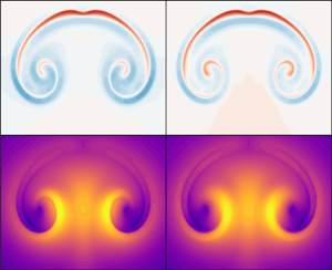
Contour plots of density (in ${\rm g}\,{\rm cm}^{-3}$) in the Rayleigh–Taylor test for models $C$ and $M_2$ at two times (a). The two simulations remain in close agreement until $t=2\,{\rm s}$, but then diverge as secondary instabilities develop. At the same time, pressure inversions appear in the horizontally averaged pressure in model $C$ (b), whereas the pressure in model $M_2$ is hydrostatic and therefore monotonic. In model $M_0$, which omits the $\dot {P}_b$ term, the pressure remains fixed at the upper and lower boundaries. (c) The evolution of the total energy in models $C$, $M_1$ and $M_2$.

Despite the eventual divergence of solutions between models $C$, $M_1$ and $M_2$, we observe quite similar energy evolution, as shown in figure 3. Model $M_2$ exhibits slightly better agreement with model $C$, although there are more significant oscillations in the gravitational and kinetic energy in model $C$. As shown in figure 2(c), model $M_2$ maintains better energy conservation than model $M_1$ up to approximately $t = 3.5\,{\rm s}$, at which point the Mach number reaches ${Ma} \simeq 0.4$. This suggests slightly better energy conservation when we include the $\bar {\lambda }$ term in our equations.

Figure 3.

Evolution of energy contributions (as described in figure 1) in the Rayleigh–Taylor test for (a) model $C$, (b) model $M_1$ and (c) model $M_2$.

4.3. Rising and falling bubbles in an atmosphere

The test cases considered so far were adiabatic, and so the ‘thermodynamically consistent’ expression for the temperature, used in model $M_3$, had no effect on the results. We now present a test case involving both prescribed heat sources and thermal diffusion, in order to elucidate the effect of this change on the model. For this case the total heating, $Q$, has the form

(4.5)\begin{equation} Q = \boldsymbol{\nabla} \boldsymbol{\cdot} \left(K\boldsymbol{\nabla} T\right) + \varPi_{t_0,t_1}(t)f(x,z), \end{equation}

where $K$ is the thermal conductivity, which we take to be constant, and $\varPi _{t_0,t_1}$ is the boxcar function, meaning that external heating is applied only for $t_0\leqslant t\leqslant t_1$. By default, thermal diffusion is implemented in MAESTROeX in terms of the specific enthalpy (Malone et al. Reference Malone, Nonaka, Almgren, Bell and Zingale2011), but for this test case we use the alternative implementation in terms of temperature, so that we can work with the corrected temperature, $T$, rather than $T_{EoS}$. This is important because, when the heating (4.5) is introduced into the heat equation (2.33), we find that

(4.6)\begin{equation} \frac{\partial}{\partial t}(\rho s) + \boldsymbol{\nabla}\boldsymbol{\cdot}(\rho s\boldsymbol{u} - K\boldsymbol{\nabla}\ln T) = K|\boldsymbol{\nabla}\ln T|^2 + \frac{1}{T}\varPi_{t_0,t_1}(t)f(x,z). \end{equation}

So thermal diffusion introduces a positive-definite source of entropy, consistent with the second law of thermodynamics.

The initial pressure and density are chosen to be

(4.7a,b)\begin{equation} P = P_0 \left(1 - z/L\right)^{{\gamma}/({\gamma-1})}, \quad \rho = \frac{1}{g}\frac{\mathrm{d} P}{\mathrm{d} z}, \end{equation}

which implies that the initial temperature, $T\propto P/\rho$, is linear in $z$ and the initial specific entropy, $s \propto \ln (P/\rho ^\gamma )$, is constant. This background state is chosen because it is steady and marginally stable to convection. The temperature gradient is fixed to its initial value at the top and bottom boundaries, so that there is no net heat flux into the domain. We use a domain of size $L_x = L_z = 2\,{\rm cm}$, with $1024 \times 1024$ grid cells. The parameter values are set as $L = 2.5\,{\rm cm}$, $P_0 = 1.65\times 10^6\,{\rm dyn}\,{\rm cm}^{-2}$, $g = -1\times 10^9\,{\rm cm}\,{\rm s}^{-2}$ and $K = 4\times 10^{4}\,{\rm erg}\,{\rm K}^{-1}\,{\rm cm}^{-1}\,{\rm s}^{-1}$.

The form of the heating function, $f(x,z)$, is chosen to produce a number of positively or negatively buoyant ‘bubbles’, via localised heat sources:

(4.8)\begin{equation} f(x,z) = \sum_i A_i \left(1 + \operatorname{tanh}(2 - |\boldsymbol{x}-\boldsymbol{x}_i|/w_i)\right), \end{equation}

with the $i$th source centred at $\boldsymbol {x}_i$, with a width $w_i$ and an amplitude $A_i$.

We first consider the case of a single rising bubble, by taking $\boldsymbol {x}_1 = (1,0.7)\,{\rm cm}$, $A_1 = 1\times 10^{13}\,{\rm erg}\,{\rm cm}^{-3}\,{\rm s}^{-1}$ and $w_1 = 0.025\,{\rm cm}$. This heating is applied between $t_0 = 1\times 10^{-5}\,{\rm s}$ and $t_1 = 2\times 10^{-5}\,{\rm s}$. Figure 4 shows close-ups of the bubble at $t = 2\times 10^{-4}\,{\rm s}$, for models $M_2$, $M_3$ and $C$; this is the time at which differences between the simulations became measurable. We do not present results from model $M_1$ because in that simulation the velocity projection failed to converge, which suggests that the $\bar {\lambda }$ term in the momentum equation is essential to this test case. Figure 4(a–c) shows temperature contours for each model; the contours for model $C$ are slightly sharper, which we attribute to the different advection scheme used in CASTRO because all of the models have the same thermal conductivity. The differences between the models are made clearer by plotting the relative temperature differences, as is done in figure 4(d–f). We see that the temperature correction introduced in model $M_3$ is positive in the vicinity of the bubble, making that bubble slightly more buoyant compared to model $M_2$. This correction to the temperature also produces a better agreement between models $M_3$ and $C$. Figure 4(g–i) shows the local Mach number in the three models, which all agree to within 1 %.

Figure 4.

Contour plots of temperature for a single rising bubble at $t = 2\times 10^{-4}\,{\rm s}$ for cases $M_2, M_3$ and $C$ (a–c). (d–f) Relative temperature differences between plots in (a–c) as indicated in each panel. (g–i) Contours of Mach number corresponding to the cases as in (a–c).

Figure 5 shows time series of energy in the same simulations. After the initial injection of heat, the total energy is conserved almost perfectly in model $C$ and to within $0.001\,\%$ in models $M_2$ and $M_3$. Cases $M_2$ and $M_3$ are essentially indistinguishable; in both cases the gravitational potential energy steadily decreases as the bubble rises, leading to an increase in kinetic energy and internal energy (through dissipative heating). The kinetic energy in model $C$ follows a very similar trajectory, as expected given the similarities in the flow seen in figure 4. However, the internal and gravitational energy terms in model $C$ exhibit a more dramatic, quasi-periodic oscillation, which we attribute to lack of hydrostatic balance in the horizontally averaged dynamics. The injection of heat in this fully compressible model establishes a gentle vertical ‘sloshing’ that is associated with very small velocities yet large changes in the internal and gravitational energy terms. In an attempt to reduce this effect, and allow a more meaningful comparison with model $C$, we have considered a second configuration with one rising bubble and one sinking bubble, as illustrated in figure 6. For this case, we place heat sources at $\boldsymbol {x}_+=(2/3,1)\,{\rm cm}$ and $\boldsymbol {x}_-=(4/3,1)\,{\rm cm}$, with amplitudes $A = \pm 2\times 10^{13}\,{\rm erg}\,{\rm cm}^{-3}\,{\rm s}^{-1}$ and the same width $w = 0.025\,{\rm cm}$. These heat sources are both applied between $t_0 = 1\times 10^{-5}\,{\rm s}$ and $t_1 = 7\times 10^{-5}\,{\rm s}$. For these simulations we use a numerical resolution of $512\times 512$ grid cells. The energy evolution for this configuration is shown in figure 7 for models $C$, $M_2$ and $M_3$. We note that the heat source and sink are not implemented exactly symmetrically, and so there is a slight drop in the total energy between times $t_0$ and $t_1$. However, after this time the total energy is conserved just as well as in the single bubble case. There are still significant fluctuations in the gravitational and internal energy in model $C$, but these are of much lower amplitude than in the single bubble case. Models $M_2$ and $M_3$ again produce very similar results, although both have a slightly lower kinetic energy than model $C$. In model $C$, as shown in figure 7(a), the gravitational potential energy remains nearly constant until $t \simeq 3\times 10^{-5}\,{\rm s}$, which is roughly equal to the sound-crossing time in the domain. Up to this time, the imposed heating produces an increase in the local fluid pressure without much change in density. In models $M_2$ and $M_3$, by contrast, the imposed heating produces an instantaneous expansion or contraction of the fluid, as dictated by the velocity constraint (3.4).

Figure 5.

Evolution of the energy for the single rising bubble test for case $C$ (a), case $M_2$ (b) and case $M_3$ (c). The plotted components are as described in figure 1. The time axis starts at $t = 1\times 10^{-5}\,{\rm s}$, when the heating is turned on.

Figure 6.

The temperature at $t=1.9\times 10^{-4}\,{\rm s}$, minus the initial temperature, in the two-bubble test with model $C$. (The results of models $M_2$ and $M_3$ are very similar.)

Figure 7.

Evolution of the energy as in figure 5, but for the rising and falling bubble test.