


1. Introduction
Surface-active agents, also referred to as surfactants, are known to have an impact on the oceans by modifying physical processes close to the air–sea interface. Surfactants have been shown to dampen ocean waves (Alpers & Hühnerfuss Reference Alpers and Hühnerfuss1989) as well as reduce the high-frequency part of the wind–wave energy spectrum (Lombardini et al. Reference Lombardini, Fiscella, Trivero, Cappa and Garrett1989). The sea surface micro layer is often populated by organic matter which creates surfactants that can modify the gas transfer velocity in specific cases (Bell et al. Reference Bell, De Bruyn, Marandino, Miller, Law, Smith and Saltzman2015). By changing the surface tension and creating surface elasticity and viscosity, surfactants change the dynamics of capillary waves and make longitudinal capillary waves possible, as investigated in the theoretical and experimental work of Lucassen (Reference Lucassen1968a,Reference Lucassenb). Surfactants have also been shown to change the dynamics of droplets and bubbles near the ocean surface (Russell et al. Reference Russell, Moore, Burrows and Quinn2023). In the subsurface region, bubble rise velocities can be modified in the presence of soluble surfactants (Takagi & Matsumoto Reference Takagi and Matsumoto2011). On the surface, surfactants can change the rate at which bubbles coalesce and pop (Néel & Deike Reference Néel and Deike2021), influence the surface residence time of bubbles and modify the droplet size distributions caused from bursting bubbles (Néel, Erinin & Deike Reference Néel, Erinin and Deike2022).
The effects of surfactants on gentle spilling breakers have been studied in the laboratory by Liu & Duncan (Reference Liu and Duncan2003, Reference Liu and Duncan2006, Reference Liu and Duncan2007). They found that surfactants can significantly change the wave breaking process by changing the shape of the wave crest and suppressing the formation of capillary waves at the onset of wave breaking. At high concentrations of surfactants, a small plunging jet was formed on the front face of the wave, entrapping a pocket of air. Using numerical simulations, Ceniceros (Reference Ceniceros2003) found that surfactants influence spilling breakers by modifying the capillary waves formed during wave breaking. It was found that this effect was caused by a marked accumulation of surfactants and high surface-tension gradients.
The dynamics of plunging breakers has been studied extensively, see e.g. Rapp & Melville (Reference Rapp and Melville1990), Perlin, He & Bernal (Reference Perlin, He and Bernal1996), Drazen, Melville & Lenain (Reference Drazen, Melville and Lenain2008), Wang, Yang & Stern (Reference Wang, Yang and Stern2016), Mostert, Popinet & Deike (Reference Mostert, Popinet and Deike2022), Erinin et al. (Reference Erinin, Liu, Wang and Duncan2023) and review articles by Banner & Peregrine (Reference Banner and Peregrine1993), Kiger & Duncan (Reference Kiger and Duncan2012) and Perlin, Choi & Tian (Reference Perlin, Choi and Tian2013). In the ocean, water is rarely free of surfactants and surface tension is often difficult to measure in the field. Additionally, breaking waves can significantly influence air–sea interaction. Despite this, virtually no studies exist on the impact of surfactants on plunging breaking water waves.
In this paper, the dynamics of plunging breakers in the presence of surfactants are studied experimentally in a wave tank. A single wave maker motion is employed to generate plunging breakers with a nominal wavelength of  $\lambda _0 = 1.18$ m using a dispersively focused wave packet technique. Two surfactant cases are studied. In the first case, the water-soluble surfactant Triton X-100 is mixed into the tank water at six bulk concentrations up to 69 % of the critical micelle concentration (CMC). In the second surfactant case, six surfactant concentrations are created by allowing naturally occurring surfactants in filtered tap water to adsorb on the water surface over various time periods up to 21 h. The surfactant-induced changes in the crest profiles at the moments of jet impact are identified and discussed with the aid of surface tension isotherms of the tank water and breaker-induced surface compression estimates from direct numerical simulations (DNS).
In § 2, the experimental set-up and measurement techniques are discussed. The results of the breaker profiles and surface tension isotherm measurements are presented in § 3. The effects of surfactants on the plunging breaker are discussed in § 4 and the conclusions are given in § 5.
2. Experimental details
2.1. Experimental facility and wave generation
Experiments were performed in the wave tank in the Hydrodynamics Laboratory at the University of Maryland. The wave tank is 14.8 m long, 1.15 m wide and 2.2 m tall, and filled with filtered tap water to a depth of 0.91 m. The tank includes a programmable wave maker consisting of a vertically oscillating wedge which spans the width of the tank at one end. A skimmer and a beach are located at the tank end opposite to the wave maker. A wind tunnel occupies the top section of the tank and is used to clean the free surface by pushing water surface contaminants towards the skimmer between runs. See details in Erinin et al. (Reference Erinin, Liu, Wang and Duncan2023).
The wave maker motion used to generate the three breakers is identical to that used to generate the ‘strong’ breaker described in Erinin et al. (Reference Erinin, Liu, Wang and Duncan2023). This wave maker motion is based on the dispersively focused wave packet technique proposed by Longuet-Higgins (Reference Longuet-Higgins1976) and used extensively by Rapp & Melville (Reference Rapp and Melville1990) and others. The wave packet has an average frequency of  $f_0 = 1.15$ Hz and, using this frequency in linear deep-water wave theory without surface tension, the nominal wavelength and phase speed are $\lambda _0 = 1.18$ m and $c_0 = 1.36\ {\rm m}\ {\rm s}^{-1}$, respectively.
2.2. Water preparation procedure
The procedures for water preparation in the wave tank for the Triton X-100 (abbreviated as TX) experiments are as follows. Before the start of the experiments, the wave tank is cleaned with bleach, rinsed thoroughly, and filled with approximately 15 000 l (a water depth of 0.91 m) of tap water filtered through a two-stage filtration system consisting of 20 and 5 micron filters. The tap water is then chlorinated to approximately 10 p.p.m. and filtered for a day through a newly replenished diatomaceous earth filter. Just before the experiments, the chlorine concentration in the tank is reduced to nearly zero by the addition of hydrogen peroxide. A low concentration of fluorescein dye is added to the tank for wave-profile measurements and visualization. Once the fluorescein dye is mixed in the tank (after approximately 3 h) the filtration system and the wind (see below) are turned off. After waiting for a period of 15 min for fluid motion to decay, a set of wave surface profiles and surface tension isotherms (see below) is collected (data set Water). After the measurements, Triton X-100 (molar mass  $M = 625\ {\rm g}\ {\rm mol}^{-1}$) is added to the tank water, and wave surface profiles and surface tension isotherm measurements are repeated on the following day. The process of adding Triton X-100 at the end of the day and taking measurements the next day is repeated a total of five times (data sets TX1 to TX5) over five consecutive days. The data for the TX6 case is collected two days after the TX5 case. The molar concentrations of Triton X-100 for the TX1 to 6 cases are 2.1, 7.5, 12.8, 34.1, 66.1, $151.0\ \mathrm {\mu }{\rm mol}\ {\rm l}^{-1}$, respectively. For comparison, the CMC of Triton X-100 is $220\ \mathrm {\mu }{\rm mol}\ {\rm l}^{-1}$, see Tiller et al. (Reference Tiller, Mueller, Dockter and Struve1984).
Six breaking wave realizations are recorded at each Triton X-100 concentration. Between successive realizations, the water-surface filtration system located inside the wind–wave tank (see Erinin et al. (Reference Erinin, Liu, Wang and Duncan2023) for details) is used to clean the water surface. The filtration system consists of a skimmer and a diatomaceous earth filter, the same filter used to initially clean the water in the tank. The in-tank filtration system is turned on for 15 min after every run. The system draws surface water through the skimmer and pumps it through the diatomaceous earth filter before returning it to the tank. The skimming is helped by a very light wind originating from the wind tunnel (close to the wave maker) and blowing in the direction towards the skimmer. After the 15 min skimming period, the filter and fans are turned off and the water in the tank is allowed to come to rest for 15 min. Just after the skimming period is terminated, a water sample ( $\approx$100 ml) is collected from the wave tank and used to measure the surface tension isotherm, see below. At the start of each day, the skimmer is operated with its outflow directed to the laboratory floor drain for a period of 30 min. Lost water by this procedure is estimated to be no more than 250 l and is replenished with freshly filtered tap water.
In the filtered tap water ageing experiments (abbreviated as Water followed by the ageing time and referred to as the Water Ageing experiments/cases), the water preparation procedure is similar to that described above, except no Triton X-100 is added to the water. After the initial surface profile and surface tension isotherm measurements (case Water as described above), the water surface is left undisturbed for a specific amount of time (2, 4, 6, 8, 11 and 21 h) and the free-surface filtration procedure is not conducted between runs. Two breaking wave realizations are recorded for each water ageing case. Although great effort is taken to remove surfactants in the Water cases, it is expected that some surfactants (from bacteria, impurities in chemicals, and other sources) would still be present in the water and/or may reach the water surface through the air. The water temperature, as measured just below the free surface, ranged from 20.5 to  $21.5\,^\circ {\rm C}$, and the relative humidity of the air, as measured at a height just above the breaking wave crest, ranged from 55 % to 60 %, respectively. The dynamic viscosity of water is assumed to be $\mu = 0.0018\ {\rm N} \ {\rm s} {\rm m}^{-2}$.
2.3. Surface profile and surface tension isotherm measurements
Two-dimensional wave surface profiles are measured using a planar laser induced fluorescence (LIF) technique that is similar to that used in Erinin et al. (Reference Erinin, Liu, Wang and Duncan2023). In the present set of experiments, the LIF images have a spatial resolution of  $227\ \mathrm {\mu }{\rm m}\ {\rm pixel}^{-1}$ and a field of view of $58.1 \times 36.3$ cm. The field of view captures the wave profile from the time before jet formation, when the wave crest becomes vertical, up to jet impact at a rate of 650 frames per second.
The surface tension isotherm is measured using a Langmuir trough system (KSV NIMA, model KN 1003) and is used to characterize the dynamic properties of the water surface. The measurements start by collecting a water sample from the wave tank (just after the filtration system is turned off before each breaker realization) and placing the sample in the trough. The sample rests in the trough for the same amount of time as the water in the wave tank from the time the skimming stops to the experimental run. The surface tension is measured with a platinum Wilhelmy plate. To measure the surface tension isotherm, the water surface in the trough is compressed by two Teflon barriers which barely touch the water surface, starting at positions at the far ends of the trough and moving towards the Wilhelmy plate at a rate of  $100\ {\rm mm}\ \min ^{-1}$ over a period of 90 s. Faster compression rates do not significantly change the measured curves of surface tension, $\sigma$, vs $A/A_0$, where $A$ is the instantaneous water surface area between the Teflon barriers and $A_0$ is its initial value. The curves of $\sigma (A/A_0)$ are recorded digitally. The Wilhelmy plate, barriers and trough are cleaned thoroughly between each measurement in the Triton X-100 experiments.
3. Results: breaking dynamics at various surfactant conditions
3.1. Surface profiles from laboratory experiments at various surfactant conditions
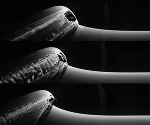
In the Water and all surfactant cases, the breaking process is qualitatively similar and begins with a steepening of the wave crest. Shortly afterwards, a small region on the front face of the wave becomes vertical and this time is referred to as the moment of jet formation. A jet then forms near the vertical section of the wave surface. This jet plunges forward and down, and impacts the water surface downstream (in the direction of wave travel) of the wave crest, entraining a pocket of air. The jet impact produces a region of large surface roughness downstream of the wave crest. Some time after jet impact, the entrained air pocket is broken up into smaller bubbles which rise to the water surface and burst. The breaking process is found to be very repeatable in the present experiments and the Water case is consistent with previous studies, see e.g. Rapp & Melville (Reference Rapp and Melville1990), Perlin et al. (Reference Perlin, He and Bernal1996), Drazen et al. (Reference Drazen, Melville and Lenain2008), and Erinin et al. (Reference Erinin, Liu, Wang and Duncan2023). The LIF movies of the breaking process for the Water and a number of surfactant cases in the present study are given as supplementary material available at https://doi.org/10.1017/jfm.2023.721.
As mentioned above, the present study is focused on the effect of surfactants on the shape of the wave crest profile at the time of jet impact. Figures 1(a) to 1(f) show LIF breaker profile images of the wave crest at the time of jet impact for filtered tap water (Water case, panel a) and various concentrations of Triton X-100 (TX1 to TX5 cases, panels b–f). In each image, the edge between the upper dark region and the lower wavy light region is the wave crest profile at the centerplane of the tank where the laser light sheet intersects the wave surface. The variation of the light intensity below this edge is due to the non-uniform intensity of the underwater portion of the light sheet, which is produced by refraction as it enters the curved water surface, and by viewing the glowing dye in the light sheet through the curved water surface between the camera and the light sheet. See Duncan et al. (Reference Duncan, Qiao, Philomin and Wenz1999) for a detailed description of these optical effects. The wave profiles obtained from these images for the Water, TX1, TX3 and TX6 cases are shown in panel (g). Interesting details in these images and profiles are the shape of the jet and the entrained air cavity, indicated by the callouts in figure 1(a). In the Water case, the entrained air cavity appears as a uniform tube of air and the surface of the jet appears smooth with a regular very small amplitude wavy pattern in the spanwise direction, that can be seen in a diagonally oriented reflection, just below the wave profile callout in figure 1(a).
Breaker profile images from high-speed movies of the wave crest and plunging jet at the time of jet impact for the Water case, in (a), and increasing concentrations of Triton X-100, TX1 to TX5 cases, in (b–f). In all cases, the breaker is created with a focused wave packet generated with the same wave maker motion. Panel (g) shows breaker profiles extracted from images at the time of jet impact, like those shown in (a–f). Only four cases are shown for clarity. The profiles are normalized by  $\lambda _0$ and aligned in the horizontal and vertical directions so that the wave crest point for each profile is at $(\tilde {x},\tilde {y}) = (0,0)$.

The shape of the wave profile changes in several important ways in the presence of Triton X-100. At the lowest concentration of surfactants, the TX1 case in figure 1(b), the jet is noticeably curled inwards, see the cyan line in panel (g), and the entrained air cavity appears irregular and perhaps broken up into many smaller bubbles. The change in the jet shape seems to be caused by a ‘spilling’ event that appears to occur under the jet as it is forming, see supplementary movies. The transition between the Water (a) and the TX1 (b) case is quite remarkable, especially given that the TX1 solution is created by adding only 17.2 ml of Triton X-100 to 15 000 l of water. As the concentration of surfactant increases in the TX2 (c) and TX3 (d) cases, the jet is still curled inwards, see green line in panel (g), and the entrained air cavity appears irregular and broken up. In the TX4 (e) case, the jet is still curled inwards; however, the entrained air cavity appears uniform as in the Water case. In the TX5 (f) case, the jet is no longer curled inwards and the air cavity appears smooth; this case appears qualitatively similar to the Water case. The TX6 case, see dark red line in panel (g), appears qualitatively similar to the TX5 and Water cases.
A transition from a laminar to an unstable jet and air cavity, like that from the Water to TX3 case, is observed in the Water to Water – 21 h cases, shown in figures 2(a) to 2(d) along with the corresponding surface profiles shown in panel (e). As mentioned above in these experiments, tank water is left undisturbed, except for making breaking waves at the above-mentioned time intervals, for the entire 21 h period. During this time, naturally occurring surfactants (probably in the bulk) are adsorbed on the free surface, changing the surface properties. The surface profile in panels (a–d) appear qualitatively similar to the transition between the Water and TX3 cases, where the entrained air cavity appears rough and broken up and the plunging jet curls inward. The curling of the plunging jet as wait time increases can be seen in the profiles in panel (e) for the Water Ageing cases. It should be noted that there is no noticeable change in the wave crest profile shapes with wait times greater than 8 h. These results show that the effects of surfactants on plunging breakers is not unique to the surfactant choice of Triton X-100. In a series of experimental studies of plunging breakers in clean water, Perlin et al. (Reference Perlin, He and Bernal1996) reported the formation of parasitic capillary waves forming on the underside of the plunging jet around the time of jet formation. Additionally, they report transverse irregularities along the jet shortly after jet formation and before jet impact. These observations may be related to the Water–TX1 transition observed in the present work and in particular the above-mentioned spilling under the jet as seen in the supplementary movies.
Breaker profile images from high-speed movies of the wave crest and plunging jet at the time of jet impact in the Water case (data recorded 15 min after turning off the filtration system) (a) and three Water Ageing experiments, from 2 to 21 h (b–d). In the Water Ageing experiments, the free surface is left undisturbed for a specified amount of time prior to the generation of the breaking waves. During this time, naturally occurring surfactants are adsorbed on the surface. The wave maker motion is the same as that used to generate the breakers in figure 1. Panel (e) shows four wave profiles aligned and normalized in the same way as the profiles in figure 1(g).

3.2. Surface tension isotherms
The Langmuir trough and the surfactant measurement results are shown in figure 3. The drawing in (a) is a schematic of the Langmuir trough used for the measurements of the surface tension isotherms, i.e. the surface tension as a function of compressed surface area,  $\sigma (A/A_0)$. See § 2.3 for a description of the device and measurement procedures. The ambient surface tension, $\sigma _0$, is taken to be the surface tension when $A/A_0 = 1$ and is plotted vs the log of the Triton X-100 concentration in panel (b). The ambient surface tension decreases linearly as concentration increases. The ambient surface tensions for the Water and Water Ageing cases are close to the surface tension of distilled water at $21\,^\circ {\rm C}$, $\sigma _d = 72.6\ {\rm mN}\ {\rm m}^{-1}$. The surface tension, $\sigma$, is plotted vs $A/A_0$ on logarithmic scale, for the Water, Triton X-100 and some of the Water Ageing cases in figure 3(c). The isotherm for the Water data with standard wait time shows an unchanging surface tension down to a compression of 75 % ( $A/A_0 = 0.25$), after which the surface tension begins to decrease at $A/A_0 \approx 0.2$ until it reaches $\sigma \approx 63\ {\rm mN}\ {\rm m}^{-1}$ at $A/A_0 = 0.12$, the largest compression used herein. In the TX1 to TX6 cases, $\sigma$ decreases continuously with decreasing $A/A_0$ and the slopes of $\sigma (A/A_0)$ decrease as bulk surfactant concentration increases.
(a) A sketch of the Langmuir trough used to measure the surface tension isotherm. The surface tension is measured by the Wilhelmy plate as the two barriers compress the water surface. The area between the barriers before the start of compression is  $A_0$. $F_s$ is equal to the surface tension times the wetted perimeter of the platinum Wilhelmy plate. The equilibrium surface tension, $\sigma _0$, where $\sigma _0 = \sigma (A/A_0 = 1)$, vs the Triton X-100 concentration, $C_{TX}$, is shown in (a) for the Triton X-100 solutions. For the Water Ageing experiments, $\sigma _0 \approx 72.4\ {\rm mN}\ {\rm m}^{-1}$, close to the value of clean water. The surface tension, $\sigma$, verses the surface area ratio in the Langmuir trough, $A/A_0$, $\sigma (A/A_0)$, is shown in (c) on a semi-log $x$-axis for Triton X-100 solutions (cases TX1 to TX6), filtered tank water (case Water), and 2, 8 and 21 h Water Ageing cases. The Water and TX1 to TX6 curves in (c) are collected from at least four measurements and the coloured contours around each curve show $\pm$1 standard deviation of $\sigma (A/A_0)$. The black horizontal dotted line in (c) is drawn at the CMC surface tension for Triton X-100, $\sigma (A/A_0) = 32\ {\rm mN}\ {\rm m}^{-1}$.

The surface tension isotherms for the Water Ageing experiments behave differently than those of the Triton X-100 cases. As mentioned previously, the Water case undoubtedly contains naturally occurring surfactants. When the water surface is left undisturbed, the surfactants have time to adsorb on the water surface. The surface tension isotherm for the Water – 2 h, 8 h and 21 h cases are shown as dashed, dotted and dash-dotted blue lines, respectively, in figure 3(c). In the Water – 2 h case, the surface tension begins to decrease at  $A/A_0 \approx 0.5$, and reaches a value of $\sigma (A/A_0 \approx 0.1) \approx 58\ {\rm mN}\ {\rm m}^{-1}$, $5\ {\rm mN}\ {\rm m}^{-1}$ less than the Water case at the same $A/A_0$. The trend continues for the 8 and 21 h cases, where the surface tension begins to decrease at a larger $A/A_0$ and reaches a smaller value at maximum compression. This result shows that surfactants which are present in the Water case can have an ambient surface tension ( $\sigma _0$) close to that of clean water, yet they can change the dynamic properties of the surface if left undisturbed over long periods of time.
The ratio of the time scales of the compression/dilatation induced by the wave to those of surfactant desorption/adsorption process from/to the water surface is of critical importance in these experiments, as it is in other wave systems such as capillary and longitudinal waves, see e.g. Lucassen (Reference Lucassen1968a,Reference Lucassenb). Two significant wave time scales are the average period of the components in the wave packet,  $T_0 = 1/f_0= 0.87$ s, and the time from the moment of jet formation to the moment of jet impact, $t_i-t_f \approx 0.15$ s. The surfactant time scales were addressed in two ways. First, isotherms at approximately TX2, TX6 and Water–23h were repeated at a compression time of $33.3$ s. Only modest changes in the isotherms were found with this faster compression rate. This is an indication that the desorption time scale is longer than the compression time. A second set of experiments was performed with Triton X-100 concentrations near the TX2 and TX6 values. In these experiments, the barriers were initially at the maximum (minimum) separation and the surfactant was at the equilibrium conditions in all cases. Compression (dilatation) was then undertaken and the barriers held at minimum (maximum) separation afterwards while surface tension was measured vs time. It was found that the surface tension vs time curves were nearly linear during at least the first five seconds after compression and that over the wave period (the larger of the above-mentioned wave time scales) the surface tension changed by a maximum of $0.13\ {\rm mN}\ {\rm m}^{-1}$ which is at most ${\approx }4$ % of the smallest difference in surface tension between equilibrium and the full compression or dilatation. All of these results indicate that wave time scale is much shorter than the surfactant desorption/adsorption time scales. Thus, the surface films are essentially insoluble during wave breaking, at least up to the time of jet impact, as considered in this work.
4. Discussion: effect of Marangoni stresses on breaking dynamics
In this section, the surface tension isotherm measurements and surface compression estimates from DNS are used to determine the surfactant characteristics that control the breaking behaviour. Attempts to correlate the jet and entrained air cavity behaviour with the ambient surface tension ( $\sigma _0$) are not successful for two reasons. First, similar transitions from a smooth jet and air cavity to a curled jet and rough air cavity occur in the Triton X-100 experiments as $\sigma _0$ varies from $72\ {\rm mN}\ {\rm m}^{-1}$ (Water) to $55\ {\rm mN}\ {\rm m}^{-1}$ (TX3) and in the wait time experiments where $\sigma _0 = 72\ \ {\rm mN}\ {\rm m}^{-1}$ in all cases. Second, in the TX cases at the highest concentration levels, TX5 and TX6 where $\sigma _0 = 43\ {\rm mN}\ {\rm m}^{-1}$ and $33\ {\rm mN}\ {\rm m}^{-1}$, respectively, the plunging jet and entrained air cavity are smooth, as they are in the Water case ( $\sigma _0=72\ {\rm mN}\ {\rm m}^{-1}$).
A possible mechanism by which surfactants can control the breaking behaviour is the combination of surface compression/dilatation induced by the wave motion and the effect of compression/dilatation on the distribution of local surface tension. For plunging breakers in water without surface tension, Longuet Higgins & Cokelet (Reference Longuet Higgins and Cokelet1976) used boundary element potential flow numerical calculations to show that there is a non-uniform compression–dilatation along the wave surface leading up to jet impact. In the present work, in order to quantify the compression/dilatation along the wave surface prior to jet impact in cases with constant surface tension, two-dimensional DNS are performed. The simulations in the present paper use the Basilisk software library to solve the two-phase Navier–Stokes equations including constant surface tension (Popinet Reference Popinet2009, Reference Popinet2015, Reference Popinet2018) and are similar to those presented in Deike, Popinet & Melville (Reference Deike, Popinet and Melville2015), Deike, Melville & Popinet (Reference Deike, Melville and Popinet2016), and Mostert et al. (Reference Mostert, Popinet and Deike2022). The numerical scheme uses a volume-of-fluid approach with a momentum-conserving advection to represent the air–liquid interface. In the simulations, the breaker is initialized as a third-order Stokes wave propagating with periodic boundary conditions, but with a large initial slope that prompts the wave to break within one wave period. The Reynolds and Bond numbers of the simulations are 100 000 and 1000, respectively, and details of the numerical set-up for this case can be found in Mostert et al. (Reference Mostert, Popinet and Deike2022). Figures 4(a) and 4(b) show the crest profiles from the experiments (Water case, blue line) and numerical simulations (black line) at the time of jet formation and impact, respectively. See figure caption for details. The experimental and DNS wave profiles appear qualitatively similar at the time of jet formation, in panel (a), and jet impact, in panel (b), when normalized by their respective wavelength.
Evaluation of surface compression–dilatation around the plunging jet from jet formation to jet impact using numerical simulations. Surface profiles from experimental measurements (Water case, blue line) and numerical simulations (black lines) at the times of jet formation and jet impact are shown in (a,b), respectively. The wavelength for the experimental profiles is taken to be  $\lambda = 2L$ where $L$ is the horizontal crest-to-trough distance at the time of jet formation. The profiles are aligned in the horizontal and vertical directions so that the wave crest point for each profile is at $(\tilde {x},\tilde {y}) = (0,0)$. The area under the plunging jet in the experiments in (b), denoted by the blue background and labelled $Q^i$, is the area enclosed by the jet face from the wave crest to the jet impact point. Panel (c) shows the time evolution of tracer particles placed $\Delta y / \lambda = 1/128$ below the water surface in the numerical simulations. Profiles I and IV are plotted at the time of jet formation and impact, respectively. The red triangles are drawn at $\pm 4$ tracer particles around the particle on the jet tip at the time of jet impact. The nine red tracer particles are used to calculate the surface compression ( $A/A_0$) up to the time of jet impact, which is plotted vs time in (d). The black vertical dashed and dotted lines in (d) are drawn at the time of jet formation and jet impact, respectively. The time axis in (d) is relative to the time of jet impact, $t_i$, and normalized by the wave period, $T$. The orange dashed lines labelled I to IV in (d) are plotted at the times of the corresponding profiles in (c).

Surface compression in the DNS is calculated by tracking 128 tracer particles placed close to the water surface and spaced evenly in  $x$ (
$x$ ( $\Delta x / \lambda = 1/128$) at a time early in the wave evolution. The results are shown in figure 4(c,d). Panel (c) shows the set of tracer particles (green and red markers) at four times from the moment of jet formation, in profile I, to jet impact, in profile IV. Each successive set of 128 points is plotted $\Delta y = 0.04$ above the previous for visualization purposes. The compression and dilatation along the jet tip in the moments leading up to jet impact can be seen clearly in figure 4(c), by the changes in spacing of the tracer particles. The red tracer particles in the four profiles in figure 4(c) are the particles that are located at the jet tip at the time of impact. Figure 4(d) shows the surface compression, $A/A_0$, of the red tracer particles vs time, where $A_0$ is taken to be the maximum tracer particle spacing some time before jet formation. It was found that the maximum surface compression experienced prior to jet impact is 90 % or $A/A_0 \approx 0.10$. Note that the results are not sensitive to the number of particles used for the averaging or small changes in the depth of the particles.
The changes in the jet shape and the air cavity observed in the two surfactant cases are thought to be the result of Marangoni stresses caused by the non-uniform compression–dilatation of surfactants on the water surface leading up to jet impact. The schematic in figure 5(a) shows a qualitative estimated of the distribution of surfactants around the time of jet formation. In this schematic, the wave is moving with a speed  $c$ to the left and surfactants concentration and surface tension gradients are expected to be highest around the wave crest and the region where the jet begins to form. It is thought that the high surface tension gradients induce local Marangoni stresses that change the wave breaking behaviour.
Panel (a) shows a representation of a wave surface profile at the time of jet formation. The orange/black objects on the water surface represent surfactant molecules. The coloured blue/orange line along the wave profile shows the change in concentration of surfactants,  $\Delta \mathcal {E}$. The highest values of $\Delta \mathcal {E}$ are expected to be along the jet tip, where the wave surface is compressed. Panel (b) shows the gradient of the surface tension, $\Delta \mathcal {E} = A_0 ({\Delta \sigma }/{\Delta A})$, computed from the surface pressure isotherms in figure 3(a). The black vertical dotted line in (b) is drawn at $A/A_0 = 0.30$. Panel (c) shows the average of $\Delta \mathcal {E}$ computed from $A/A_0 = 1$ to $0.30$ for the Water, TX1 to 6 and Water – 2 h, 8 h, 21 h (shown in $+$,
$+$,  $\times$ and $\ast$) cases and plotted vs Triton X-100 concentration, $C_{TX}$. The inset photos of the surface profiles in (c) are also shown in figure 1 and discussed in § 3.1. Panel (d) shows $\overline {Q_i}$, the area under the upper surface of the plunging jet at impact vs Marangoni number, Ma. The vertical error bars in (d) show $\pm$1 standard deviation for the TX cases, where six runs are conducted for each condition. A sample measurement of $Q_i$ is shown in figure 4(b). The blue and orange background colours in (d) show regions where the plunging jet is smooth and irregular, respectively, and the white colour indicates the transition. Panels (e,f) show the surface tracer particles obtained from DNS, the same ones shown in figure 4(c). Each tracer particle close to the wave crest is coloured according to the gradient of surface tension along the wave surface, $\Delta \sigma / \Delta s$, as computed from the surface tension isotherms for the TX1 (e) and TX6 (f) cases and DNS results. The variable s is the arc length along the wave profile.

In order to estimate the magnitude of the Marangoni stresses in the different surfactant conditions, the surface tension gradient,  $\Delta \mathcal {E} = A_0 ({\Delta \sigma }/{\Delta A})$, is first calculated from the surface pressure isotherms. The variable $\Delta \mathcal {E}$ is analogous to the Gibbs elasticity, $E = A (\mathrm {d}\sigma / \mathrm {d}A)$ (Manikantan & Squires Reference Manikantan and Squires2020) and a higher value of $\Delta \mathcal {E}$ suggests a greater tendency of the surface to resist compression. Figure 5(b) shows $\Delta \mathcal {E}$ plotted vs $A/A_0$. The curves of $\Delta \mathcal {E}(A/A_0)$ for the TX1 to TX6 cases all show a nearly linear increase as the surface is compressed. Among these cases, the highest and smallest (almost zero) rates of increase in $\Delta \mathcal {E}$ occur in the TX1 and TX6 cases, respectively. In the Water case, $\Delta \mathcal {E}$ is close to zero until 75 % compression ( $A/A_0 = 0.25$), after which it starts to increase at an almost monotonic rate. The Water Ageing – 2 h, 8 h and 21 h cases display qualitative similarities to the Water case, except that the value of $A/A_0$ at which $\Delta \mathcal {E}$ begins to increase gradually shifts from 0.25 to 0.8 as the wait time increases.
The impact of Marangoni stresses on the plunging jet is evaluated by calculating the average gradient of the surface tension,  $\overline {\Delta \mathcal {E}}$, from $A/A_0 = 1$ to $0.30$. The lower limit of $A/A_0 = 0.30$ is chosen based on results from the DNS. A plot of $\overline {\Delta \mathcal {E}}$ vs Triton X-100 concentration, $C_{TX}$, is shown in figure 5(c). The curve of $\overline {\Delta \mathcal {E}}(C_{TX})$ exhibits a sharp increase from the Water to the TX1 case, rising from approximately $1\ {\rm mN}\ {\rm m}^{-1}$ to around $23\ {\rm mN}\ {\rm m}^{-1}$. Among the surfactant cases, the TX1 case displays the highest value of $\overline {\Delta \mathcal {E}}$, which gradually decreases as the Triton X-100 concentration increases from TX2 to TX6, ultimately reaching a final value of approximately $3\ {\rm mN}\ {\rm m}^{-1}$ for the TX6 case. The values of $\overline {\Delta \mathcal {E}}$ are found to be non-monotonic with increases of surfactant concentration, with the highest values of $\overline {\Delta \mathcal {E}}$ observed for low Triton X-100 concentrations. For the Water Ageing experiments, shown as blue markers in figure 5(c), the value of $\overline {\Delta \mathcal {E}}$ is found to increase monotonically with wait time.
The sharp increase in  $\overline {\Delta \mathcal {E}}$ observed between the Water and TX1 experiments, followed by a subsequent decrease for higher values of $C_{TX}$, corresponds to the smooth–irregular–smooth transition of the plunging jet discussed in § 3.1. These findings indicate that the surfactants’ effects on the shape of the plunging breaker are correlated with $\overline {\Delta \mathcal {E}}$. For instance, when $\overline {\Delta \mathcal {E}}$ is relatively low, below approximately $3\ {\rm mN}\ {\rm m}^{-1}$ as observed in the Water and TX6 cases, the surface profiles are smooth. On the other hand, when $\overline {\Delta \mathcal {E}}$ is high, exceeding $5\ {\rm mN}\ {\rm m}^{-1}$ as seen in the TX1 to TX4 cases, the elevated Marangoni stresses alter the geometry of the jet by inducing inward curling and significantly reducing the entrained air cavity. It is speculated that the lower surface tension values at the jet tip and higher values on the upper and lower surfaces of the plunging jet, implied by the combined experiments and DNS results, exert a net force approximately in the direction from the jet tip toward the wave crest. It should be noted that an additional set of Water Ageing, Water and TX1 to TX6 experiments were conducted (not shown in this manuscript) under the same conditions except that the overall wave maker amplitude was smaller than that used in this paper, i.e. the ‘weak’ breaker from Erinin et al. (Reference Erinin, Liu, Wang and Duncan2023). In those experiments, it was observed that a plunging breaker formed at low values of $\overline {\Delta \mathcal {E}}$ and a spilling breaker formed at high values of $\overline {\Delta \mathcal {E}}$.
A Marangoni number for the flow field is defined as  $Ma = \overline {\Delta \mathcal {E}}/(\mu c_0)$. This Marangoni number definition is consistent with the definition found in Manikantan & Squires (Reference Manikantan and Squires2020) since $c_0$, the nominal wave phase speed defined in § 2, is a characteristic speed of the motion of the surface. Figure 5(d) shows the geometric parameter $\overline {Q_i}$ as a function of $Ma$ where two regimes are observed. The first regime is when $Ma < 2$ and $\overline {Q_i} \approx 3500\ {\rm mm}^2$, which coincides with a smooth jet surface and a large value of $\overline {Q_i}$. The second regime is when $Ma > 3$ and $\overline {Q_i} \approx 2500\ {\rm mm}^2$, which coincides with an irregularly shaped jet surface.
In order to illustrate the strength of the Marangoni stresses in the experiments, the surface compression from the simulations can be combined with the experimental measurements of  $\sigma (A/A_0)$ to compute $\Delta \sigma / \Delta s$, the hypothetical Marangoni stresses due to the local surface compression along the wave surface, $s$, in the DNS. It should be emphasized that surfactants are not represented in the DNS. The results are shown in figure 5(e,f). In each panel, the tracer particles from figures 4(c) and 4(d) are coloured according to the local value of $\Delta \sigma / \Delta s$. In the TX1 case (e), $\Delta \sigma / \Delta s$ has a significant non-zero value in the crest/plunging jet region from the time of jet formation lasting until jet impact, while in the TX6 case, $\Delta \sigma /\Delta s \approx 0$ at all surface locations and times. These results serve as further evidence that the surface tension gradients play a key role in the differences observed in the different surfactant cases.
5. Conclusion
The effects of surfactants on breaking waves is studied experimentally in two types of surfactant solutions: filtered tap water with various concentrations of Triton X-100 and filtered tap water aged for 15 min (called the Water case) to 21 h. In the Water case, which has very low surfactant levels, the jet moves forward and falls onto the water surface, creating an entrained air pocket upon impact with a smooth jet face and air cavity. The presence of surfactants dramatically alters the wave breaking process, changing the shape of the jet and wave crest profile during jet impact, particularly at low Triton X-100 concentrations and for the 2 to 21 h Water Ageing experiments. As the Triton X-100 concentration is further increased, the jet shape and entrained air cavity progressively resemble those observed in the filtered tap water case. Close to the Triton X-100 CMC, the jet and entrained air cavity show qualitative and quantitative similarities to the filtered tap water case.
Differences in the surfactant cases are thought to be the result of Marangoni stresses caused by surface compression of the surfactants. The ambient surface tension,  $\sigma _0$, is found to play a secondary role. The surface compression on a plunging breaker is evaluated using 2-D DNS with constant surface tension and the water surface around the jet tip is found to compress by as much as 90 %. Using the surface tension isotherm at each surfactant concentration and guided by the DNS results, the average surface tension gradient, $\overline {\Delta \mathcal {E}}$, is computed for each case. It is found that $\overline {\Delta \mathcal {E}}$ is low for the Water case and the surfactant cases close to the CMC and high for the low to intermediate surfactant concentration and Water Ageing cases. The changes in the wave crest at the time of jet impact are shown to correlate with $\overline {\Delta \mathcal {E}}$ between the time of jet formation and impact. As an example, the area under the upper surface of the plunging jet at impact is plotted vs the Marangoni number, $Ma = \overline {\Delta \mathcal {E}}/(\mu c_0)$. It is found that when the Marangoni number is $\lessapprox$2, the jet and entrained air cavity appear smooth and the area under the plunging jet is large. When $Ma$ is greater than 3, the jet and entrained air cavity appear irregular and the area under the plunging jet is reduced by approximately 30 %. In order to evaluate the surface tension gradient ( $\Delta \sigma / \Delta s$) distribution along each wave profile, the DNS and surface tension isotherms are combined. The results show that $\Delta \sigma / \Delta s$ is high along the wave crest and near the jet tip in each case, and increases with increasing $\overline {\Delta \mathcal {E}}$.
Supplementary movies
Supplementary movies are available at https://doi.org/10.1017/jfm.2023.721.
Funding
The support of the Division of Ocean Sciences of the National Science Foundation under grant OCE1849762 to L.D. and OCE1925060 to J.H.D. and X.L. are gratefully acknowledged.
Declaration of interests
The authors report no conflict of interest.
Author contributions
M.A.E. and J.H.D. designed the experiments. M.A.E. and C.L. collected the data and analysed it with input from J.H.D., L.D. and X.L. The simulations were performed by W.M. The paper was written by M.A.E. with the help of J.H.D. and L.D. All authors edited the paper.


 Open access