


1. Introduction
Vortex-induced vibration (VIV) is a prominent phenomenon across multiple engineering fields, influencing structures such as heat exchanger tubes, offshore risers, bridges, chimneys and marine vessels. These vibrations result from the interaction between fluid flow and structural components, where vortex formation leads to large-amplitude oscillations, potentially causing significant damage to engineering structures. Foundational studies on VIV have been extensively reviewed by Sarpkaya (Reference Sarpkaya1979), Griffin & Ramberg (Reference Griffin and Ramberg1982), Bearman (Reference Bearman1984), Parkinson (Reference Parkinson1989) and Williamson & Govardhan (Reference Williamson and Govardhan2004).
The VIV response of a circular cylinder and the associated wake flow dynamics are influenced by various parameters. Specifically, the mass ratio $m^*$
, which is the ratio of structural oscillating mass to the mass displaced by the fluid, plays a key role in determining the onset and extent of VIV. Prior work by Govardhan & Williamson (Reference Govardhan and Williamson2002) identified a critical mass ratio around 0.54, below which large-amplitude VIV can persist indefinitely, a phenomenon referred to as ‘VIV forever’. This phenomenon has been confirmed in both experimental and numerical studies, showing that, as long as the mass ratio remains below this critical value, the system continues to experience large-amplitude oscillations across a wide range of inflow velocities (Shiels, Leonard & Roshko Reference Shiels, Leonard and Roshko2001; Ryan, Thompson & Hourigan Reference Ryan, Thompson and Hourigan2005; Han et al. Reference Han, De Langre, Thompson, Hourigan and Zhao2023). Another important factor is the structural damping ratio
$m^*$
, which is the ratio of structural oscillating mass to the mass displaced by the fluid, plays a key role in determining the onset and extent of VIV. Prior work by Govardhan & Williamson (Reference Govardhan and Williamson2002) identified a critical mass ratio around 0.54, below which large-amplitude VIV can persist indefinitely, a phenomenon referred to as ‘VIV forever’. This phenomenon has been confirmed in both experimental and numerical studies, showing that, as long as the mass ratio remains below this critical value, the system continues to experience large-amplitude oscillations across a wide range of inflow velocities (Shiels, Leonard & Roshko Reference Shiels, Leonard and Roshko2001; Ryan, Thompson & Hourigan Reference Ryan, Thompson and Hourigan2005; Han et al. Reference Han, De Langre, Thompson, Hourigan and Zhao2023). Another important factor is the structural damping ratio $\zeta$
, which affects both the amplitude and lock-in region of VIV. Generally, increasing structural damping decreases the amplitude of vibrations and reduces the lock-in range (Blevins & Coughran Reference Blevins and Coughran2009; Soti et al. Reference Soti, Zhao, Thompson, Sheridan and Bhardwaj2018). The combination of mass and damping ratios represented by
$\zeta$
, which affects both the amplitude and lock-in region of VIV. Generally, increasing structural damping decreases the amplitude of vibrations and reduces the lock-in range (Blevins & Coughran Reference Blevins and Coughran2009; Soti et al. Reference Soti, Zhao, Thompson, Sheridan and Bhardwaj2018). The combination of mass and damping ratios represented by $(m^* + C_{\!A})\zeta$
has been thoroughly discussed and demonstrated to govern VIV response in studies by Khalak & Williamson (Reference Khalak and Williamson1999) and Govardhan & Williamson (Reference Govardhan and Williamson2006). Here,
$(m^* + C_{\!A})\zeta$
has been thoroughly discussed and demonstrated to govern VIV response in studies by Khalak & Williamson (Reference Khalak and Williamson1999) and Govardhan & Williamson (Reference Govardhan and Williamson2006). Here, $C_{\!A}\approx 1$
is the added-mass coefficient. Early studies of VIV focused on scenarios with high mass and damping, revealing two amplitude response branches identified as: (i) an ‘initial’ branch, corresponding to the highest amplitudes at low reduced velocities, and (ii) a ‘lower’ branch with decreasing amplitudes at high reduced velocities (Feng Reference Feng1968; Brika & Laneville Reference Brika and Laneville1993). Here, the reduced velocity is defined as
$C_{\!A}\approx 1$
is the added-mass coefficient. Early studies of VIV focused on scenarios with high mass and damping, revealing two amplitude response branches identified as: (i) an ‘initial’ branch, corresponding to the highest amplitudes at low reduced velocities, and (ii) a ‘lower’ branch with decreasing amplitudes at high reduced velocities (Feng Reference Feng1968; Brika & Laneville Reference Brika and Laneville1993). Here, the reduced velocity is defined as $U^* = U_0/(f_{\textit{n}}\text{D})$
, where
$U^* = U_0/(f_{\textit{n}}\text{D})$
, where $U_0$
represents the flow velocity,
$U_0$
represents the flow velocity, $f_n$
is the structural natural frequency and
$f_n$
is the structural natural frequency and $D$
is the cylinder’s diameter. In contrast to high mass-damping cases, the experiments by Khalak & Williamson (Reference Khalak and Williamson1996, Reference Khalak and Williamson1997, Reference Khalak and Williamson1999) revealed the existence of another branch of response called the ‘upper branch’, situated between the ‘initial’ and ‘lower’ branches when the mass-damping ratio is low. It is worth noting that, for VIV of flexible risers with multiple natural frequency modes, the vibration amplitude can exhibit more than one local maximum region with the growth of reduced velocity (Bourguet, Karniadakis & Triantafyllou Reference Bourguet, Karniadakis and Triantafyllou2011; Seyed-Aghazadeh & Modarres-Sadeghi Reference Seyed-Aghazadeh and Modarres-Sadeghi2018; Huera-Huarte Reference Huera-Huarte2025).
$D$
is the cylinder’s diameter. In contrast to high mass-damping cases, the experiments by Khalak & Williamson (Reference Khalak and Williamson1996, Reference Khalak and Williamson1997, Reference Khalak and Williamson1999) revealed the existence of another branch of response called the ‘upper branch’, situated between the ‘initial’ and ‘lower’ branches when the mass-damping ratio is low. It is worth noting that, for VIV of flexible risers with multiple natural frequency modes, the vibration amplitude can exhibit more than one local maximum region with the growth of reduced velocity (Bourguet, Karniadakis & Triantafyllou Reference Bourguet, Karniadakis and Triantafyllou2011; Seyed-Aghazadeh & Modarres-Sadeghi Reference Seyed-Aghazadeh and Modarres-Sadeghi2018; Huera-Huarte Reference Huera-Huarte2025).
The understanding of VIV is rooted in the energy transfer between fluid and structure, which is governed by the phase relationship between unsteady fluid loads and the structural response. This interaction produces feedback between the body’s motion and the vortices it generates, resulting in various wake patterns and dynamic behaviours. Govardhan & Williamson (Reference Govardhan and Williamson2000) closely examined these transitions between the three branches and the wake dynamics of VIV, revealing two distinct phase shifts and frequency transitions in low mass-damping systems. Specifically, at low reduced velocities in the initial branch, the phase angle is small (close to zero), with fluid forces and structure motion nearly in phase and the cylinder exhibiting small-amplitude vibrations. The cylinder wake flow features the ‘2S’ vortex mode (two single vortices per cycle). As the reduced velocity increases, a sudden phase shift occurs during the transition to the upper branch, where the wake mode changes from ‘2S’ to ‘2P’ (two pairs of vortices per cycle), which is associated with a substantial increase in vibration amplitude. This first phase shift, known as the ‘vortex phase’ jump, occurs when the vibration frequency approaches the system’s natural frequency in water. Further increases in reduced velocity lead to the transition from the upper to lower branch, where another significant phase angle shift occurs. This second phase shift, termed the ‘total phase’ jump, occurs when the vibration frequency reaches the natural frequency in a vacuum (Govardhan & Williamson Reference Govardhan and Williamson2000). It is worth noting that the VIV response and vortex-shedding mode mentioned above are primarily investigated under single degree-of-freedom (DOF) vibrations transverse to the flow. Williamson & Jauvtis (Reference Williamson and Jauvtis2004) pointed out that, when significant in-line motion occurs, the transverse vibrations can also be amplified, with the peak-to-peak VIV amplitude up to 3 times the cylinder diameter. In this scenario, the wake flow features a triplet of vortices produced per half-vibration cycle, which is defined as the ‘2T’ mode.
Although most studies of VIV have focused on scenarios with steady incoming flow speed, offshore structures such as risers and pipelines are frequently impinged by wave-induced hydrodynamic loads where the flow velocity exhibits sinusoidal oscillations (Fredsoe & Sumer Reference Fredsoe and Sumer1997; Sarpkaya Reference Sarpkaya1977). In such oscillatory flow environments, the hydrodynamic forces and flow characteristics are highly influenced by the Keulegan–Carpenter (KC) number (Keulegan & Carpenter Reference Keulegan and Carpenter1958) defined as $\textit{KC} = {U_m T}/{D}$
. Here,
$\textit{KC} = {U_m T}/{D}$
. Here, $U_m$
is the amplitude of the oscillatory flow velocity, and
$U_m$
is the amplitude of the oscillatory flow velocity, and $T$
is the oscillatory flow period. At very low
$T$
is the oscillatory flow period. At very low $\textit{KC}$
values with
$\textit{KC}$
values with $\textit{KC}\lt 1$
, the flow remains attached and two-dimensional (Stokes Reference Stokes1851; Wang Reference Wang1968). As
$\textit{KC}\lt 1$
, the flow remains attached and two-dimensional (Stokes Reference Stokes1851; Wang Reference Wang1968). As $\textit{KC}$
increases up to 4, Honji (Reference Honji1981) documented the emergence of three-dimensional instabilities caused by centrifugal forces in the boundary layer, marking the transition to chaotic and turbulent states, referred to as Honji vortices by Sarpkaya (Reference Sarpkaya1986). Williamson (Reference Williamson1985) reported that further increases in
$\textit{KC}$
increases up to 4, Honji (Reference Honji1981) documented the emergence of three-dimensional instabilities caused by centrifugal forces in the boundary layer, marking the transition to chaotic and turbulent states, referred to as Honji vortices by Sarpkaya (Reference Sarpkaya1986). Williamson (Reference Williamson1985) reported that further increases in $\textit{KC}$
produce various vortex-shedding regimes. The VIV response of circular cylinders in these pure oscillatory flows was investigated by several studies. Sumer & Fredsøe (Reference Sumer and Fredsøe1988) studied the transverse vibrations of a cylinder in oscillating flow over
$\textit{KC}$
produce various vortex-shedding regimes. The VIV response of circular cylinders in these pure oscillatory flows was investigated by several studies. Sumer & Fredsøe (Reference Sumer and Fredsøe1988) studied the transverse vibrations of a cylinder in oscillating flow over $ 5 \lt \textit{KC} \lt 100$
, where the vibration amplitude exhibited multiple local maxima as a function of inflow oscillation intensity. A similar phenomenon was reported by following studies via numerical simulations (Zhao, Cheng & An Reference Zhao, Cheng and An2012; Zhao Reference Zhao2013; Fu, Zou & Wan Reference Fu, Zou and Wan2018; Zhu et al. Reference Zhu, Xu, Liu and Zhong2024). Specifically, Zhu et al. (Reference Zhu, Xu, Liu and Zhong2024) identified different types of vortex interactions, including splitting, merging, combined splitting–merging and dissipation. In addition, Thorsen, Sævik & Larsen (Reference Thorsen, Sævik and Larsen2016) published a time-domain semi-empirical method for predicting the cylinder response in oscillatory flows based on their previously developed model for steady-flow cases (Thorsen et al. Reference Thorsen, Sævik and Larsen2014, Reference Thorsen, Sævik and Larsen2015). Lu et al. (Reference Lu, Fu, Zhang and Ren2019) proposed a time-domain prediction model to inspect the VIV response of flexible risers under unsteady flows.
$ 5 \lt \textit{KC} \lt 100$
, where the vibration amplitude exhibited multiple local maxima as a function of inflow oscillation intensity. A similar phenomenon was reported by following studies via numerical simulations (Zhao, Cheng & An Reference Zhao, Cheng and An2012; Zhao Reference Zhao2013; Fu, Zou & Wan Reference Fu, Zou and Wan2018; Zhu et al. Reference Zhu, Xu, Liu and Zhong2024). Specifically, Zhu et al. (Reference Zhu, Xu, Liu and Zhong2024) identified different types of vortex interactions, including splitting, merging, combined splitting–merging and dissipation. In addition, Thorsen, Sævik & Larsen (Reference Thorsen, Sævik and Larsen2016) published a time-domain semi-empirical method for predicting the cylinder response in oscillatory flows based on their previously developed model for steady-flow cases (Thorsen et al. Reference Thorsen, Sævik and Larsen2014, Reference Thorsen, Sævik and Larsen2015). Lu et al. (Reference Lu, Fu, Zhang and Ren2019) proposed a time-domain prediction model to inspect the VIV response of flexible risers under unsteady flows.
In contrast to VIV in pure steady or oscillatory flows as reviewed above, the cylinder vibration response under combined current–oscillatory flows encompasses a much larger parameter space, including inflow oscillation intensity (the proportion of flow oscillation amplitude with respect to mean flow velocity), frequency ratio (the ratio between flow oscillation frequency to structural natural frequency) and reduced velocity. A limited number of studies have touched upon this issue. Zhao et al. (Reference Zhao, Kaja, Xiang and Yan2013) investigated the VIV of a circular cylinder subjected to combined steady and oscillatory flows using two-dimensional Reynolds-averaged Navier–Stokes equations under different inflow oscillation intensities with a fixed $\textit{KC}=10$
. The study reported that in combined flows at flow ratios (the proportion of steady flow in the total flow velocity) between 0.4 and 0.6, the lock-in range is much wider than in steady or pure oscillatory flows. At a flow ratio of 0.8, the cylinder showed its highest cross-flow vibration intensity, reaching 1.5 diameters in the ‘super upper’ branch. Vortex-shedding patterns also varied with flow, shifting from ‘2S’ to ‘2P’ and then ‘2T’ as reduced velocity increased, leading to large vibrations and beating effects. Recent numerical simulations of VIV in purely oscillatory flows by Dorogi, Baranyi & Konstantinidis (Reference Dorogi, Baranyi and Konstantinidis2023) at large KC numbers have revealed pronounced hysteresis in amplitude and frequency response between flow acceleration and deceleration stages, they demonstrated that the response remains fundamentally non-quasi-steady even when the flow variation is extremely slow. Ulveseter et al. (Reference Ulveseter, Thorsen, Sævik and Larsen2018) proposed a semi-empirical prediction tool to characterise the vibrations of risers under combined irregular waves and uniform current, which demonstrated reasonable agreement with experimental measurements. Their model successfully predicted both total response (wave + VIV frequencies) and filtered VIV-only signals, and showed that waves dampen in-line VIV while cross-flow vibrations remain largely unaffected. Despite these advances, fundamental questions remain unresolved: What is the frequency structure underlying the observed amplitude beating? How do flow oscillation parameters (intensity and frequency) independently control the multi-frequency response? What governs the non-quasi-steady coupling between instantaneous flow velocity, hydrodynamic forces and vortex dynamics? Recent methodological advances have begun to address some related challenges. Fu et al. (Reference Fu, Fu, Zhang, Han, Ren, Xu and Zhao2022) numerically demonstrated frequency capture in tandem cylinders with different diameters, where the downstream cylinder’s response is dominated by upstream vortex-shedding frequency, with energy transfer occurring from vorticity to structure rather than through typical VIV mechanisms. Building on these findings, Zhao et al. (Reference Zhao, Zhang, Fu, Fu, Ren and Xu2023) developed an empirical drag coefficient prediction model for tandem unequal-diameter flexible cylinders through experimental investigation, incorporating a modified wake model and accounting for VIV/wake-induced vibrations amplification effects, spacing ratios and diameter differences. Li & Chen (Reference Li and Chen2025) developed a coupled VIV prediction method for flexible risers conveying severe slug flow using a modified wake oscillator model with Computational Fluid Dynamics (CFD) analysis, they found that mode transition occurs under high-velocity sheared flow or high KC number oscillatory flow, and severe slug flow induces distinct multi-frequency phenomena and higher-order mode responses absent in conventional straight-flow riser systems.
$\textit{KC}=10$
. The study reported that in combined flows at flow ratios (the proportion of steady flow in the total flow velocity) between 0.4 and 0.6, the lock-in range is much wider than in steady or pure oscillatory flows. At a flow ratio of 0.8, the cylinder showed its highest cross-flow vibration intensity, reaching 1.5 diameters in the ‘super upper’ branch. Vortex-shedding patterns also varied with flow, shifting from ‘2S’ to ‘2P’ and then ‘2T’ as reduced velocity increased, leading to large vibrations and beating effects. Recent numerical simulations of VIV in purely oscillatory flows by Dorogi, Baranyi & Konstantinidis (Reference Dorogi, Baranyi and Konstantinidis2023) at large KC numbers have revealed pronounced hysteresis in amplitude and frequency response between flow acceleration and deceleration stages, they demonstrated that the response remains fundamentally non-quasi-steady even when the flow variation is extremely slow. Ulveseter et al. (Reference Ulveseter, Thorsen, Sævik and Larsen2018) proposed a semi-empirical prediction tool to characterise the vibrations of risers under combined irregular waves and uniform current, which demonstrated reasonable agreement with experimental measurements. Their model successfully predicted both total response (wave + VIV frequencies) and filtered VIV-only signals, and showed that waves dampen in-line VIV while cross-flow vibrations remain largely unaffected. Despite these advances, fundamental questions remain unresolved: What is the frequency structure underlying the observed amplitude beating? How do flow oscillation parameters (intensity and frequency) independently control the multi-frequency response? What governs the non-quasi-steady coupling between instantaneous flow velocity, hydrodynamic forces and vortex dynamics? Recent methodological advances have begun to address some related challenges. Fu et al. (Reference Fu, Fu, Zhang, Han, Ren, Xu and Zhao2022) numerically demonstrated frequency capture in tandem cylinders with different diameters, where the downstream cylinder’s response is dominated by upstream vortex-shedding frequency, with energy transfer occurring from vorticity to structure rather than through typical VIV mechanisms. Building on these findings, Zhao et al. (Reference Zhao, Zhang, Fu, Fu, Ren and Xu2023) developed an empirical drag coefficient prediction model for tandem unequal-diameter flexible cylinders through experimental investigation, incorporating a modified wake model and accounting for VIV/wake-induced vibrations amplification effects, spacing ratios and diameter differences. Li & Chen (Reference Li and Chen2025) developed a coupled VIV prediction method for flexible risers conveying severe slug flow using a modified wake oscillator model with Computational Fluid Dynamics (CFD) analysis, they found that mode transition occurs under high-velocity sheared flow or high KC number oscillatory flow, and severe slug flow induces distinct multi-frequency phenomena and higher-order mode responses absent in conventional straight-flow riser systems.
Despite the efforts mentioned above, our knowledge of cylinder vibration patterns and vortex-shedding modes within combined current–oscillatory flow environments across various reduced velocities, frequency ratios and inflow oscillation intensities remains limited. In particular, the coupling between instantaneous incoming flow velocity, multi-frequency VIV responses and time-varying hydrodynamic loads, as well as their impacts on vortex generation and transport in wake flow, is far from well understood. The primary aim of this study is to elucidate the fundamental fluid–structure interaction mechanisms governing cross-flow VIV of a circular cylinder subjected to combined steady current and sinusoidally oscillating flows. Through systematic water-channel experiments and theoretical interpretations, we highlight the impact of unsteady incoming flows on modulating multi-frequency vibration components and causing deviations of the VIV response from quasi-steady predictions under diverse frequency ratios, inflow oscillation intensities and reduced velocities ranging from the initial to lower response branches.
This manuscript is organised as follows. The experimental set-up and the parameter space investigated in this work are described in § 2. Baseline cylinder VIV response under steady flows are discussed in § 3. Cross-flow cylinder vibration patterns, hydrodynamic load analysis and the associated vortex dynamics are illustrated in § 4. Theoretical interpretations for the evolution of multi-frequency VIV components are demonstrated in § 5. Finally, the principal conclusions are given in § 6.
(a) Basic schematic of the experimental set-up illustrating the vibration system, oscillatory flow generator and particle image velocimetry system. (b) Two-dimensional layout of the schematic and the origin location in quiescent flow.

2. Experiment set-up
The experiments were performed in a recirculation water channel at the University of Texas at Dallas with a test section of 2 m length and 0.2 m width. The channel was operated with a free surface and water depth of $h_w=0.18$
m. The background turbulence intensity of this channel is less than 1
$h_w=0.18$
m. The background turbulence intensity of this channel is less than 1 $\,\%$
. An acrylic circular cylinder with diameter
$\,\%$
. An acrylic circular cylinder with diameter $D = 25$
mm and length
$D = 25$
mm and length $L = 194$
mm was horizontally mounted on an oscillating platform and fully submerged in water, resulting in an averaged blockage ratio of 13.9 %. Brankovic (Reference Brankovic2004) and Morse & Williamson (Reference Morse and Williamson2009) reported that blockage ratios (BRs) of up to 15 % have only minor effects on VIV response, primarily causing a small reduction in amplitude at lock-in. To further assess the influence of blockage ratio on cylinder vibration response, supplementary experiments were performed at two additional water depths of
$L = 194$
mm was horizontally mounted on an oscillating platform and fully submerged in water, resulting in an averaged blockage ratio of 13.9 %. Brankovic (Reference Brankovic2004) and Morse & Williamson (Reference Morse and Williamson2009) reported that blockage ratios (BRs) of up to 15 % have only minor effects on VIV response, primarily causing a small reduction in amplitude at lock-in. To further assess the influence of blockage ratio on cylinder vibration response, supplementary experiments were performed at two additional water depths of $h_w=0.17$
and 0.19 m, corresponding to averaged blockage ratios
$h_w=0.17$
and 0.19 m, corresponding to averaged blockage ratios $\textit{BR} = D/h_w$
of 14.7 % and 13.4 %, respectively. The results show that despite the minor difference in the VIV amplitudes, the dynamic response trends remain consistent with
$\textit{BR} = D/h_w$
of 14.7 % and 13.4 %, respectively. The results show that despite the minor difference in the VIV amplitudes, the dynamic response trends remain consistent with $\textit{BR}$
varying from 13.4 % to 14.7 %. Details of the sensitivity test for VIV response to the BR are presented in the Supplementary Materials (§ 5) is available at https://doi.org/10.1017/jfm.2026.11418.
$\textit{BR}$
varying from 13.4 % to 14.7 %. Details of the sensitivity test for VIV response to the BR are presented in the Supplementary Materials (§ 5) is available at https://doi.org/10.1017/jfm.2026.11418.
The cylinder was positioned in the centre of the channel with a 3 mm gap from each side of the channel sidewalls to mitigate the three-dimensional vortex shedding from the cylinder tips. Both ends of the cylinder were connected to aluminium plates with 1 mm thickness and then attached to piston rods running through air bearings (figure 1). The entire system was stabilised using two linear springs with a spring stiffness of $k = 6.3$
N m−1, which led to a natural frequency of the oscillation system of
$k = 6.3$
N m−1, which led to a natural frequency of the oscillation system of $f_n = 1.128$
Hz determined through free-decay tests in air. The mass ratio of this set-up,
$f_n = 1.128$
Hz determined through free-decay tests in air. The mass ratio of this set-up, $m^*$
, calculated by the total mass of all moving parts connected to the testing cylinder divided by the mass of displaced water, was 2.6. With a constant pressure supply to the air bearings, this vibrating system achieved a structural damping ratio of
$m^*$
, calculated by the total mass of all moving parts connected to the testing cylinder divided by the mass of displaced water, was 2.6. With a constant pressure supply to the air bearings, this vibrating system achieved a structural damping ratio of $\zeta = 0.73\,\%$
. This resulted in a mass-damping factor of
$\zeta = 0.73\,\%$
. This resulted in a mass-damping factor of $(m^* + C_{\!A})\zeta = 0.027$
(
$(m^* + C_{\!A})\zeta = 0.027$
( $C_{\!A} = 1$
is the added-mass coefficient), categorised under the low mass-damping regime as defined by Govardhan & Williamson (Reference Govardhan and Williamson2000).
$C_{\!A} = 1$
is the added-mass coefficient), categorised under the low mass-damping regime as defined by Govardhan & Williamson (Reference Govardhan and Williamson2000).
In this work, the periodically oscillating inflow was produced via a movable mesh frame system positioned 460 mm downstream of the testing cylinder. A stainless mesh composed of 130 $\unicode{x03BC}$
m diameter wires and a bulk porosity of 60
$\unicode{x03BC}$
m diameter wires and a bulk porosity of 60 $\,\%$
was mounted on a high-torque motor driven transverse system to allow periodic streamwise oscillations. The movement of this mesh frame was controlled via the Laboratory Virtual Instrument Engineering Workbench system with adjustable oscillation intensities and frequencies. The physical mechanism relies on periodic modulation of the channel’s hydraulic resistance. As the mesh oscillates streamwise, it alters the effective resistance and creates pressure fluctuations that propagate upstream through flow continuity. The downstream mesh placement prevents upstream turbulence introduction, and combined with the recirculated water tunnel design with upstream flow-diverging–converging design, ensures that cylinder wake interactions do not contaminate the inflow. This enabled the production of sinusoidal water velocity fluctuations at the location of the testing cylinder, where the instantaneous incoming flow velocity is expressed as
$\,\%$
was mounted on a high-torque motor driven transverse system to allow periodic streamwise oscillations. The movement of this mesh frame was controlled via the Laboratory Virtual Instrument Engineering Workbench system with adjustable oscillation intensities and frequencies. The physical mechanism relies on periodic modulation of the channel’s hydraulic resistance. As the mesh oscillates streamwise, it alters the effective resistance and creates pressure fluctuations that propagate upstream through flow continuity. The downstream mesh placement prevents upstream turbulence introduction, and combined with the recirculated water tunnel design with upstream flow-diverging–converging design, ensures that cylinder wake interactions do not contaminate the inflow. This enabled the production of sinusoidal water velocity fluctuations at the location of the testing cylinder, where the instantaneous incoming flow velocity is expressed as $u(t) = U_0 (1 + \sigma \sin (2\pi f_w t))$
. Here,
$u(t) = U_0 (1 + \sigma \sin (2\pi f_w t))$
. Here, $U_0$
is the mean velocity generated by the channel pump,
$U_0$
is the mean velocity generated by the channel pump, $\sigma$
is the flow oscillation intensity and
$\sigma$
is the flow oscillation intensity and $f_w$
is the oscillation frequency. Figure 2 illustrates the representative time series of incoming water flow velocities at various spanwise and wall-normal locations after phase averaging. In general, the periodically oscillating inflow generated by this movable mesh frame system exhibited minor deviations in oscillation intensity and phase across both the spanwise and wall-normal locations. Further analysis with phase-averaged velocity distributions demonstrated that the relative divergence from the ideal sinusoidal velocity profile is in general less than 3 % across one complete oscillation cycle, indicating that this movable mesh frame system is capable of reproducing the desired sinusoidal flow conditions. In the following discussion, the inflow velocity data were extracted from a spatial averaging region located upstream of the cylinder, spanning
$f_w$
is the oscillation frequency. Figure 2 illustrates the representative time series of incoming water flow velocities at various spanwise and wall-normal locations after phase averaging. In general, the periodically oscillating inflow generated by this movable mesh frame system exhibited minor deviations in oscillation intensity and phase across both the spanwise and wall-normal locations. Further analysis with phase-averaged velocity distributions demonstrated that the relative divergence from the ideal sinusoidal velocity profile is in general less than 3 % across one complete oscillation cycle, indicating that this movable mesh frame system is capable of reproducing the desired sinusoidal flow conditions. In the following discussion, the inflow velocity data were extracted from a spatial averaging region located upstream of the cylinder, spanning $-2.0 \leq x/D \leq -1.5$
in the streamwise direction and
$-2.0 \leq x/D \leq -1.5$
in the streamwise direction and $-2.0 \leq y/D \leq 2.0$
in the cross-stream direction (the origin
$-2.0 \leq y/D \leq 2.0$
in the cross-stream direction (the origin $(x,y)=(0,0)$
denotes to the cylinder centre at equilibrium position).
$(x,y)=(0,0)$
denotes to the cylinder centre at equilibrium position).
A sample case of the phase-averaged time series of the incoming flow at various wall-normal and spanwise locations for $U_0^*$
= 4.98,
$U_0^*$
= 4.98, $\sigma$
= 0.16 and
$\sigma$
= 0.16 and $f_w/f_n$
= 0.18. The green dashed line represents the relative deviation between the measured flow velocity and the desired sinusoidal profile at the origin of the coordinate system defined as
$f_w/f_n$
= 0.18. The green dashed line represents the relative deviation between the measured flow velocity and the desired sinusoidal profile at the origin of the coordinate system defined as $\varepsilon _u=1-u/[ U_0(1 + \sigma \sin (2\pi f_w t))]$
.
$\varepsilon _u=1-u/[ U_0(1 + \sigma \sin (2\pi f_w t))]$
.

The vibrations and associated wake flow dynamics of the circular cylinder under periodically oscillating inflows are expected to be highly modulated by the inflow conditions, including mean flow speed $U_0$
, flow fluctuation intensity
$U_0$
, flow fluctuation intensity $\sigma$
and frequency
$\sigma$
and frequency $f_w$
. To reveal the impacts of each parameter on fluid–structure interactions, the experimental campaigns were categorised into three groups. In the first baseline group, the VIV of the circular cylinder was characterised under steady-flow environments (i.e.
$f_w$
. To reveal the impacts of each parameter on fluid–structure interactions, the experimental campaigns were categorised into three groups. In the first baseline group, the VIV of the circular cylinder was characterised under steady-flow environments (i.e. $\sigma =0$
and
$\sigma =0$
and $f_w=0$
) with the mean flow speed in the range
$f_w=0$
) with the mean flow speed in the range $U_0 \in [0.08,0.33]$
m s
$U_0 \in [0.08,0.33]$
m s $^{-1}$
at intervals of every
$^{-1}$
at intervals of every $\Delta U_0=0.0066$
m s
$\Delta U_0=0.0066$
m s $^{-1}$
, which corresponded to Reynolds numbers
$^{-1}$
, which corresponded to Reynolds numbers $\textit{Re} = U_0D/\nu \in [2000,8300]$
or reduced velocities
$\textit{Re} = U_0D/\nu \in [2000,8300]$
or reduced velocities $U^* = U_0/(f_{\textit{n}}\text{D}) \in [2.88,11.77]$
. The second group focused on the impact of inflow fluctuation intensity on VIV responses. In this group, the flow fluctuation frequency was fixed at
$U^* = U_0/(f_{\textit{n}}\text{D}) \in [2.88,11.77]$
. The second group focused on the impact of inflow fluctuation intensity on VIV responses. In this group, the flow fluctuation frequency was fixed at $f_w/f_n=0.18$
, and three inflow velocity fluctuation intensities
$f_w/f_n=0.18$
, and three inflow velocity fluctuation intensities $\sigma = 0.16, 0.23 \text{ and } 0.30$
were explored. The third group characterised the role of inflow fluctuation frequency on cylinder vibrations, by varying
$\sigma = 0.16, 0.23 \text{ and } 0.30$
were explored. The third group characterised the role of inflow fluctuation frequency on cylinder vibrations, by varying $f_w/f_n$
at 0.27, 0.35 and 0.44 while fixing
$f_w/f_n$
at 0.27, 0.35 and 0.44 while fixing $\sigma = 0.30$
. The experimental parameter space is summarised in table 1. It is worth noting that, for the second and third groups, cases under high reduced velocities were not included to mitigate the disturbance of the surface wave on the desired oscillatory velocity profiles. Following the criterion proposed by Bishop & Hassan (Reference Bishop and Hassan1964), the impact of surface wave can be characterised by the maximum Froude number, defined as
$\sigma = 0.30$
. The experimental parameter space is summarised in table 1. It is worth noting that, for the second and third groups, cases under high reduced velocities were not included to mitigate the disturbance of the surface wave on the desired oscillatory velocity profiles. Following the criterion proposed by Bishop & Hassan (Reference Bishop and Hassan1964), the impact of surface wave can be characterised by the maximum Froude number, defined as
 \begin{equation} \textit{Fr}_{\textit{max}} = \frac {U_{\textit{max}}}{\sqrt {\textit{gh}_{\textit{min}}}}, \end{equation}
where $U_{\textit{max}}$
is the maximum mean flow velocity,
$U_{\textit{max}}$
is the maximum mean flow velocity, $g$
is the gravitational acceleration and
$g$
is the gravitational acceleration and $h_{\textit{min}}$
is the minimum clearance from the top of the vibrating cylinder to the free surface. The parameter space inspected in the second and third groups yielded
$h_{\textit{min}}$
is the minimum clearance from the top of the vibrating cylinder to the free surface. The parameter space inspected in the second and third groups yielded $\textit{Fr}_{\textit{max}}\approx 0.38$
, which is close to the
$\textit{Fr}_{\textit{max}}\approx 0.38$
, which is close to the $\textit{Fr}_{\textit{max}}$
= 0.375 value in the experiment by Bishop & Hassan (Reference Bishop and Hassan1964). Previous studies have suggested that surface wave effects are negligible when
$\textit{Fr}_{\textit{max}}$
= 0.375 value in the experiment by Bishop & Hassan (Reference Bishop and Hassan1964). Previous studies have suggested that surface wave effects are negligible when $\textit{Fr}_{\textit{max}} \lesssim 0.5$
(Sareen et al. Reference Sareen, Zhao, Sheridan, Hourigan and Thompson2018). Therefore, the influence of the free surface is neglected in the subsequent analysis. Additional information for the calculation of time-varying
$\textit{Fr}_{\textit{max}} \lesssim 0.5$
(Sareen et al. Reference Sareen, Zhao, Sheridan, Hourigan and Thompson2018). Therefore, the influence of the free surface is neglected in the subsequent analysis. Additional information for the calculation of time-varying $\textit{Fr}(t)$
during cylinder vibration and its distribution under the highest
$\textit{Fr}(t)$
during cylinder vibration and its distribution under the highest $U_0$
is provided in the Supplementary Material § 4.
$U_0$
is provided in the Supplementary Material § 4.
Experimental parameter space summary with submergence and Froude number characteristics.

The flow-induced vibrations of the cylinder were captured using a Dantec high-speed camera with 1920 $\times$
1200 px resolution operating at 60 Hz. To enhance visibility, the cylinder’s surface was painted with a fiducial mark. The instantaneous position of the cylinder was then extracted via image processing by detecting the geometrical centre of the fiducial mark in each frame (Gong, Bhamitipadi Suresh & Jin Reference Gong, Bhamitipadi Suresh and Jin2023). Based on the camera resolution of 4.2 pixels per mm, the uncertainty in cylinder displacement was approximately 240
$\times$
1200 px resolution operating at 60 Hz. To enhance visibility, the cylinder’s surface was painted with a fiducial mark. The instantaneous position of the cylinder was then extracted via image processing by detecting the geometrical centre of the fiducial mark in each frame (Gong, Bhamitipadi Suresh & Jin Reference Gong, Bhamitipadi Suresh and Jin2023). Based on the camera resolution of 4.2 pixels per mm, the uncertainty in cylinder displacement was approximately 240 $\unicode{x03BC}$
m, which was less than 1
$\unicode{x03BC}$
m, which was less than 1 $\,\%$
of the cylinder diameter. The hydrodynamic forces acting on the vibrating cylinder were calculated indirectly from the measured cylinder displacement using the governing equations of motion ((3.1) and (3.2)). From the cylinder displacement, the velocity
$\,\%$
of the cylinder diameter. The hydrodynamic forces acting on the vibrating cylinder were calculated indirectly from the measured cylinder displacement using the governing equations of motion ((3.1) and (3.2)). From the cylinder displacement, the velocity $\dot {y}(t)$
and acceleration
$\dot {y}(t)$
and acceleration $\ddot {y}(t)$
were numerically derived using central difference schemes. The total hydrodynamic force
$\ddot {y}(t)$
were numerically derived using central difference schemes. The total hydrodynamic force $F_t(t)$
and vortex force
$F_t(t)$
and vortex force $F_v(t)$
were then calculated by rearranging the governing equations. A time-resolved, planar particle image velocimetry (PIV) system from TSI was utilised to quantify the coupling between incoming flow velocity, circular cylinder vibrations and wake flow dynamics. A field of view of 200 mm
$F_v(t)$
were then calculated by rearranging the governing equations. A time-resolved, planar particle image velocimetry (PIV) system from TSI was utilised to quantify the coupling between incoming flow velocity, circular cylinder vibrations and wake flow dynamics. A field of view of 200 mm $\times$
135 mm (8.0D
$\times$
135 mm (8.0D $\times$
5.4D) was illuminated by a 1 mm thick laser sheet from a 30 mJ/pulse laser, with the coordinate origin located at the centre of the circular cylinder in its equilibrium position with the water at rest. To facilitate the flow visualisation, silver-coated hollow glass spheres with a diameter of 14
$\times$
5.4D) was illuminated by a 1 mm thick laser sheet from a 30 mJ/pulse laser, with the coordinate origin located at the centre of the circular cylinder in its equilibrium position with the water at rest. To facilitate the flow visualisation, silver-coated hollow glass spheres with a diameter of 14 $\unicode{x03BC}$
m and density of 1.02 g cm
$\unicode{x03BC}$
m and density of 1.02 g cm $^{-3}$
were seeded in the water flow. Before each experiment, the cylinder was allowed to reach steady VIV for at least 20 s, then the oscillatory flow was allowed to reach its steady state for at least 80 s. The flow field and cylinder displacements were then captured using a 4 MP (2560
$^{-3}$
were seeded in the water flow. Before each experiment, the cylinder was allowed to reach steady VIV for at least 20 s, then the oscillatory flow was allowed to reach its steady state for at least 80 s. The flow field and cylinder displacements were then captured using a 4 MP (2560 $\times$
1600 pixels), 16-bit CMOS camera at 60 Hz for at least 12 inflow oscillation cycles. A convergence study was performed to validate the statistical reliability of this choice by comparing phase-averaged quantities computed from 10, 12 and 14 cycles (see Supplementary Material § 3). The results demonstrated good convergence that 12 cycles provide statistically reliable measurements for the flow conditions investigated. The instantaneous velocities were derived from the image pairs using a recursive cross-correlation method via the INSIGHT 4G software from TSI. The interrogation window size was 32 pixels with a 50
$\times$
1600 pixels), 16-bit CMOS camera at 60 Hz for at least 12 inflow oscillation cycles. A convergence study was performed to validate the statistical reliability of this choice by comparing phase-averaged quantities computed from 10, 12 and 14 cycles (see Supplementary Material § 3). The results demonstrated good convergence that 12 cycles provide statistically reliable measurements for the flow conditions investigated. The instantaneous velocities were derived from the image pairs using a recursive cross-correlation method via the INSIGHT 4G software from TSI. The interrogation window size was 32 pixels with a 50 $\,\%$
overlap, resulting in a final vector grid spacing of
$\,\%$
overlap, resulting in a final vector grid spacing of $\Delta x = \Delta y = 1.89$
mm. This methodology ensured that more than 95
$\Delta x = \Delta y = 1.89$
mm. This methodology ensured that more than 95 $\,\%$
of the vectors were valid on average. The overall uncertainty in particle location identification was approximately 0.1 pixel, corresponding to an uncertainty in velocity measurement of approximately 1.7
$\,\%$
of the vectors were valid on average. The overall uncertainty in particle location identification was approximately 0.1 pixel, corresponding to an uncertainty in velocity measurement of approximately 1.7 $\,\%$
, considering a bulk particle displacement of approximately 6 pixels between successive images.
$\,\%$
, considering a bulk particle displacement of approximately 6 pixels between successive images.
The primary sources of experimental uncertainty include imaging resolution for displacement measurements and PIV velocity measurements. Table 2 summarises the propagated uncertainties for key quantities at typical upper-branch conditions. The cylinder displacement measured via high-speed imaging has an uncertainty of $\delta y = 0.24$
mm, corresponding to approximately 1 % of the cylinder diameter. The PIV velocity measurements exhibit a relative uncertainty of 1.7 %. Through standard error propagation using root-sum-square methods, the derived quantities show the following relative uncertainties near
$\delta y = 0.24$
mm, corresponding to approximately 1 % of the cylinder diameter. The PIV velocity measurements exhibit a relative uncertainty of 1.7 %. Through standard error propagation using root-sum-square methods, the derived quantities show the following relative uncertainties near $U^* \approx 5.0$
: the normalised amplitude
$U^* \approx 5.0$
: the normalised amplitude $A/D$
has 0.8 % uncertainty, the total force coefficient
$A/D$
has 0.8 % uncertainty, the total force coefficient $\hat {C}_t$
has 4.7 % uncertainty, the vortex-force coefficient
$\hat {C}_t$
has 4.7 % uncertainty, the vortex-force coefficient $\hat {C}_v$
has 4.6 % uncertainty and the reduced velocity
$\hat {C}_v$
has 4.6 % uncertainty and the reduced velocity $U^*$
has 1.9 % uncertainty. Detailed derivations of all uncertainty calculations are provided in Supplementary Material § 1.
$U^*$
has 1.9 % uncertainty. Detailed derivations of all uncertainty calculations are provided in Supplementary Material § 1.
Experimental uncertainties for typical upper-branch conditions near $U^* \approx 5.0$
. Detailed derivations are provided in Supplementary Material § 1.
$U^* \approx 5.0$
. Detailed derivations are provided in Supplementary Material § 1.

To assess the repeatability of the imposed oscillatory inflow, cycle-to-cycle variability was quantified through analysis of multiple consecutive flow oscillation cycles at a representative condition ( $U_0^* = 4.98$
,
$U_0^* = 4.98$
, $\sigma = 0.16$
,
$\sigma = 0.16$
, $f_w/f_n = 0.18$
). Time-resolved PIV measurements across the domain were segmented into individual cycles, and each cycle was fitted to extract local oscillation amplitude
$f_w/f_n = 0.18$
). Time-resolved PIV measurements across the domain were segmented into individual cycles, and each cycle was fitted to extract local oscillation amplitude $\sigma$
and phase
$\sigma$
and phase $\phi _w$
. Statistical analysis of various representative spatial locations distributed across the measurement domain shows that the normalised oscillation amplitude deviations remain within 5 %, with cycle-to-cycle standard deviations less than 4 %. Phase variations exhibit standard deviations of approximately
$\phi _w$
. Statistical analysis of various representative spatial locations distributed across the measurement domain shows that the normalised oscillation amplitude deviations remain within 5 %, with cycle-to-cycle standard deviations less than 4 %. Phase variations exhibit standard deviations of approximately $2^\circ$
–
$2^\circ$
– $4^\circ$
, demonstrating good temporal stability and spatial uniformity of the imposed flow conditions. Complete repeatability analysis including contour fields and tabulated statistics is provided in Supplementary Material § 2.
$4^\circ$
, demonstrating good temporal stability and spatial uniformity of the imposed flow conditions. Complete repeatability analysis including contour fields and tabulated statistics is provided in Supplementary Material § 2.
3. Baseline group: VIV of circular cylinder under steady flows
To validate the experimental set-up and facilitate the understanding of VIV mechanisms in subsequent experiments under unsteady-flow conditions, the VIV response from the baseline group (i.e. VIV within steady incoming water flows) was firstly examined. Figure 3 summarises the vibration amplitude, frequency, load coefficients and phase angle between the cylinder displacement and the fluid load at various reduced velocities $U^*$
. Similar to previous studies (Blevins Reference Blevins1977), the VIV amplitude
$U^*$
. Similar to previous studies (Blevins Reference Blevins1977), the VIV amplitude $A/D$
shown in figure 3(a) was determined by calculating the standard deviation of the cylinder displacement and amplifying by
$A/D$
shown in figure 3(a) was determined by calculating the standard deviation of the cylinder displacement and amplifying by $\sqrt {2}$
to approximately represent the average amplitude over multiple cycles of steady-state oscillations. Overall, the evolution of VIV amplitudes aligns well with those reported in previous experimental studies by Khalak & Williamson (Reference Khalak and Williamson1997), Assi, Bearman & Meneghini (Reference Assi, Bearman and Meneghini2010) and Lin et al. (Reference Lin, Sun, Liu, Zhu, Wang, Triantafyllou and Fan2024) under similar mass-damping parameters
$\sqrt {2}$
to approximately represent the average amplitude over multiple cycles of steady-state oscillations. Overall, the evolution of VIV amplitudes aligns well with those reported in previous experimental studies by Khalak & Williamson (Reference Khalak and Williamson1997), Assi, Bearman & Meneghini (Reference Assi, Bearman and Meneghini2010) and Lin et al. (Reference Lin, Sun, Liu, Zhu, Wang, Triantafyllou and Fan2024) under similar mass-damping parameters $m^*\zeta$
, where a distinctive increase of
$m^*\zeta$
, where a distinctive increase of $A/D$
occurs in the low
$A/D$
occurs in the low $U^*$
region and the maximum
$U^*$
region and the maximum $A/D$
reaches
$A/D$
reaches $0.8 \pm 0.1$
. It is worth noting that the cylinder was released to vibrate from a quiescent condition under each
$0.8 \pm 0.1$
. It is worth noting that the cylinder was released to vibrate from a quiescent condition under each $U^*$
. To test the influence of the path-dependent effect on VIV response, supplementary experiments were performed under both rising and falling
$U^*$
. To test the influence of the path-dependent effect on VIV response, supplementary experiments were performed under both rising and falling $U^*$
conditions within
$U^*$
conditions within $3.8 \leq U^* \leq 6$
. The results are detailed in the Supplementary Materials in § 6. Overall, the VIV amplitude exhibits a minor path-dependent effect. Recent study by Liu et al. (Reference Liu, Gao, Liu and Qi2025) pointed out that the reduction of the mass-damping ratio mitigates the path-dependent effect phenomenon between the initial and upper branches. In our work, the small
$3.8 \leq U^* \leq 6$
. The results are detailed in the Supplementary Materials in § 6. Overall, the VIV amplitude exhibits a minor path-dependent effect. Recent study by Liu et al. (Reference Liu, Gao, Liu and Qi2025) pointed out that the reduction of the mass-damping ratio mitigates the path-dependent effect phenomenon between the initial and upper branches. In our work, the small $m^*\zeta$
at
$m^*\zeta$
at $1.9\times 10^{-2}$
aligns with the low path-dependent effect. The dominant modes of cylinder vibrations across
$1.9\times 10^{-2}$
aligns with the low path-dependent effect. The dominant modes of cylinder vibrations across $U^*$
are illustrated in figure 3(b) via the compensated spectra
$U^*$
are illustrated in figure 3(b) via the compensated spectra $P/\max \{P\}$
, where
$P/\max \{P\}$
, where $P$
represents the spectrum of the cylinder displacements. In general, VIV of the circular cylinder exhibits a dominant frequency in the vicinity of
$P$
represents the spectrum of the cylinder displacements. In general, VIV of the circular cylinder exhibits a dominant frequency in the vicinity of $f_n$
with moderate growth as a function of
$f_n$
with moderate growth as a function of $U^*$
. A similar trend was likewise observed in previous studies (Khalak & Williamson Reference Khalak and Williamson1997; Assi et al. Reference Assi, Bearman and Meneghini2010; Lin et al. Reference Lin, Sun, Liu, Zhu, Wang, Triantafyllou and Fan2024).
$U^*$
. A similar trend was likewise observed in previous studies (Khalak & Williamson Reference Khalak and Williamson1997; Assi et al. Reference Assi, Bearman and Meneghini2010; Lin et al. Reference Lin, Sun, Liu, Zhu, Wang, Triantafyllou and Fan2024).
(a) Cross-flow VIV response of the circular cylinder under steady inflows. The amplitude $A/D$
represents the VIV amplitude normalised by the cylinder diameter. The dashed lines mark the three classical response branches: initial, upper and lower. The insets illustrate representative displacement time series corresponding to each branch. The amplitude curve of
$A/D$
represents the VIV amplitude normalised by the cylinder diameter. The dashed lines mark the three classical response branches: initial, upper and lower. The insets illustrate representative displacement time series corresponding to each branch. The amplitude curve of $A/D$
is compared with previous studies by Khalak & Williamson (Reference Khalak and Williamson1997), Assi et al. (Reference Assi, Bearman and Meneghini2010) and Lin et al. (Reference Lin, Sun, Liu, Zhu, Wang, Triantafyllou and Fan2024); (b) normalised power spectrum of cylinder displacement; (c) total (
$A/D$
is compared with previous studies by Khalak & Williamson (Reference Khalak and Williamson1997), Assi et al. (Reference Assi, Bearman and Meneghini2010) and Lin et al. (Reference Lin, Sun, Liu, Zhu, Wang, Triantafyllou and Fan2024); (b) normalised power spectrum of cylinder displacement; (c) total ( $\hat {C_t}$
) and vortex (
$\hat {C_t}$
) and vortex ( $\hat {C_v}$
) load coefficients defined by (3.1) and (3.2). The error bar represents the uncertainty level of load coefficients; (d) evolution of total phase angle
$\hat {C_v}$
) load coefficients defined by (3.1) and (3.2). The error bar represents the uncertainty level of load coefficients; (d) evolution of total phase angle $\phi$
and vortex phase angle
$\phi$
and vortex phase angle $\phi _v$
across
$\phi _v$
across $U^*$
, which characterises the transition between three branches.
$U^*$
, which characterises the transition between three branches.

The calculation of the phase angle between the cylinder displacement and the fluid loads is achieved through the governing equation of cylinder displacements. Specifically, assuming one-DOF harmonic vibration, the equation of motion can be expressed as
 \begin{equation} m\ddot {y} + c\dot {y} + ky = F_{t}(t)=\frac {1}{2}\rho U_0^2 \textit{DL}\hat {C_t} \sin (2\pi \textit{ft} + \phi ), \end{equation}
where $y$
,
$y$
, $\dot {y}$
and
$\dot {y}$
and $\ddot {y}$
denote the displacement, velocity and acceleration of the body, respectively. Here,
$\ddot {y}$
denote the displacement, velocity and acceleration of the body, respectively. Here, $F_{t}(t)$
is the total fluid force and
$F_{t}(t)$
is the total fluid force and $\hat {C_t}$
is the corresponding force coefficient. The phase angle
$\hat {C_t}$
is the corresponding force coefficient. The phase angle $\phi$
describes the phase relationship between the cross-flow fluid force and the displacement. As pointed out by Lighthill (Reference Lighthill1986), the total fluid force can be further decomposed into a potential force component derived from the added mass
$\phi$
describes the phase relationship between the cross-flow fluid force and the displacement. As pointed out by Lighthill (Reference Lighthill1986), the total fluid force can be further decomposed into a potential force component derived from the added mass $F_{p}(t) = -({C_{\!A}\pi \rho D^2 L}/{4}) \ddot {y}(t)$
, and a vortex-force component
$F_{p}(t) = -({C_{\!A}\pi \rho D^2 L}/{4}) \ddot {y}(t)$
, and a vortex-force component $F_v(t)$
. This allows the governing equation of VIV to be reorganised into the form
$F_v(t)$
. This allows the governing equation of VIV to be reorganised into the form
 \begin{equation} \left(m + \frac {C_{\!A}\pi \rho D^2 L}{4}\right) \ddot {y} + c \dot {y} + k y = F_{v}(t)=\frac {1}{2}\rho U_0^2 \textit{DL}\hat {C_v} \sin (2\pi \textit{ft} + \phi _v), \end{equation}
where $\hat {C_v}$
is the vortex-force coefficient and
$\hat {C_v}$
is the vortex-force coefficient and $\phi _v$
represents the phase difference between the cylinder displacement and the vortex force.
$\phi _v$
represents the phase difference between the cylinder displacement and the vortex force.
Vortex formation modes under steady flow at $U^*=3.58$
(a,b);
$U^*=3.58$
(a,b); $U^*=4.76$
(c,d); and
$U^*=4.76$
(c,d); and $U^*=8.27$
(e, f), corresponding to the three distinct vibration branches. The cylinders are shown at their peak displacement locations.
$U^*=8.27$
(e, f), corresponding to the three distinct vibration branches. The cylinders are shown at their peak displacement locations.

Following (3.1) and (3.2), the evolutions of $\phi$
,
$\phi$
, $\phi _v$
,
$\phi _v$
, $\hat {C_t}$
and
$\hat {C_t}$
and $\hat {C_v}$
across
$\hat {C_v}$
across $U^*$
are summarised in figure 3(c,d). Both
$U^*$
are summarised in figure 3(c,d). Both $\phi$
and
$\phi$
and $\phi _v$
remain close to
$\phi _v$
remain close to $0^\circ$
at low
$0^\circ$
at low $U^*$
, then exhibit a nearly
$U^*$
, then exhibit a nearly $180^\circ$
jump when
$180^\circ$
jump when $U^*$
increases to 3.8 and 5.8, respectively. The evolution of the phase difference between the cylinder displacement and the fluid loads allows the VIV response to be categorised into three branches: the initial branch (
$U^*$
increases to 3.8 and 5.8, respectively. The evolution of the phase difference between the cylinder displacement and the fluid loads allows the VIV response to be categorised into three branches: the initial branch ( $U^* \leq 3.8$
, with
$U^* \leq 3.8$
, with $\phi \approx 0^\circ$
and
$\phi \approx 0^\circ$
and $\phi _v \approx 0^\circ$
), the upper branch (
$\phi _v \approx 0^\circ$
), the upper branch ( $4 \leq U^* \lt 5.8$
, with
$4 \leq U^* \lt 5.8$
, with $\phi \approx 0^\circ$
and
$\phi \approx 0^\circ$
and $\phi _v \approx 180^\circ$
) and the lower branch (
$\phi _v \approx 180^\circ$
) and the lower branch ( $U^* \geq 5.8$
, with
$U^* \geq 5.8$
, with $\phi \approx 180^\circ$
and
$\phi \approx 180^\circ$
and $\phi _v \approx 180^\circ$
). Notably, the upper branch is characterised by the occurrence of large VIV amplitudes and elevated fluid load magnitudes,
$\phi _v \approx 180^\circ$
). Notably, the upper branch is characterised by the occurrence of large VIV amplitudes and elevated fluid load magnitudes, $\hat {C_t}$
and
$\hat {C_t}$
and $\hat {C_v}$
. As pointed out by Govardhan & Williamson (Reference Govardhan and Williamson2000), the variations of
$\hat {C_v}$
. As pointed out by Govardhan & Williamson (Reference Govardhan and Williamson2000), the variations of $\phi$
and
$\phi$
and $\phi _v$
between each branch are associated with the modulation of vortex-shedding patterns. This phenomenon is reflected in representative phase-averaged vorticity distributions from the PIV measurements in figure 4. Specifically, within the initial branch, the wake flow is dominated by a single pair vortex production within one cylinder vibration cycle (i.e. ‘2S’ mode). When
$\phi _v$
between each branch are associated with the modulation of vortex-shedding patterns. This phenomenon is reflected in representative phase-averaged vorticity distributions from the PIV measurements in figure 4. Specifically, within the initial branch, the wake flow is dominated by a single pair vortex production within one cylinder vibration cycle (i.e. ‘2S’ mode). When $U^*$
increases to the upper and lower branches, two vortex pairs are formed per VIV cycle (i.e. ‘2P’ mode), and the strength of the secondary vortex from each pair is higher within the lower branch. In summary, both the cylinder vibration patterns and vortex-shedding modes from the baseline cases (i.e. VIV in steady flows) are found in good agreement with previous experimental works (Govardhan & Williamson Reference Govardhan and Williamson2000; Assi et al. Reference Assi, Bearman and Meneghini2010; Lin et al. Reference Lin, Sun, Liu, Zhu, Wang, Triantafyllou and Fan2024) under similar mass-damping ratios.
$U^*$
increases to the upper and lower branches, two vortex pairs are formed per VIV cycle (i.e. ‘2P’ mode), and the strength of the secondary vortex from each pair is higher within the lower branch. In summary, both the cylinder vibration patterns and vortex-shedding modes from the baseline cases (i.e. VIV in steady flows) are found in good agreement with previous experimental works (Govardhan & Williamson Reference Govardhan and Williamson2000; Assi et al. Reference Assi, Bearman and Meneghini2010; Lin et al. Reference Lin, Sun, Liu, Zhu, Wang, Triantafyllou and Fan2024) under similar mass-damping ratios.
4. Cross-flow cylinder vibration under combined current–oscillatory flows
In this section, we investigate the vibration patterns of the elastically mounted circular cylinder under periodically oscillating flows across various flow oscillation intensities $\sigma$
and frequencies
$\sigma$
and frequencies $f_w$
. The results highlight the non-quasi-steady coupling between instantaneous incoming flow velocity and the cylinder response. Next, we will endeavour to elucidate the unsteady vortex production and transport patterns induced by cylinder vibrations under combined current–oscillatory flows. Special focus will be placed on the temporal variations of vortex-shedding modes and their coupling with the non-quasi-steady VIV response as a function of instantaneous inflow velocity. The discussions will be divided into two parts: the influence of incoming flow oscillation intensity
$f_w$
. The results highlight the non-quasi-steady coupling between instantaneous incoming flow velocity and the cylinder response. Next, we will endeavour to elucidate the unsteady vortex production and transport patterns induced by cylinder vibrations under combined current–oscillatory flows. Special focus will be placed on the temporal variations of vortex-shedding modes and their coupling with the non-quasi-steady VIV response as a function of instantaneous inflow velocity. The discussions will be divided into two parts: the influence of incoming flow oscillation intensity $\sigma$
and frequency
$\sigma$
and frequency $f_w$
.
$f_w$
.
Cylinder vibration response at fixed inflow oscillation frequency $f_w/f_n = 0.18$
under various oscillation intensities
$f_w/f_n = 0.18$
under various oscillation intensities $\sigma$
. (a) Normalised vibration amplitude
$\sigma$
. (a) Normalised vibration amplitude $A/D$
; (b) amplitude difference
$A/D$
; (b) amplitude difference $A-A_{\textit{QS}}$
between the experimental results and the quasi-steady estimations.
$A-A_{\textit{QS}}$
between the experimental results and the quasi-steady estimations.

4.1. Impact of incoming flow oscillation intensity on VIV response
A first assessment of the impact of flow oscillation intensity $\sigma$
on the cylinder’s response patterns is given with the vibration amplitude
$\sigma$
on the cylinder’s response patterns is given with the vibration amplitude $A/D$
across
$A/D$
across $U^*$
summarised in figure 5(a). For all scenarios with oscillating incoming flows, the reduced velocity
$U^*$
summarised in figure 5(a). For all scenarios with oscillating incoming flows, the reduced velocity $U^*$
was calculated based on the mean flow speed
$U^*$
was calculated based on the mean flow speed $U_0$
, and
$U_0$
, and $A/D$
was determined from the time series of cylinder displacement with the same approach as discussed in the baseline group section. Results displayed in figure 5 reveal that, despite the velocity oscillations from incoming flow, the cylinder vibration amplitude pattern exhibits a similar trend in comparison with the baseline group, where
$A/D$
was determined from the time series of cylinder displacement with the same approach as discussed in the baseline group section. Results displayed in figure 5 reveal that, despite the velocity oscillations from incoming flow, the cylinder vibration amplitude pattern exhibits a similar trend in comparison with the baseline group, where $A/D$
increases significantly at
$A/D$
increases significantly at $U^*\approx 3.8$
and gradually decays within
$U^*\approx 3.8$
and gradually decays within $U^*\gt 6$
. Notably, the growth of
$U^*\gt 6$
. Notably, the growth of $\sigma$
gradually mitigates the maximum cylinder vibration amplitude, which drops from 0.72
$\sigma$
gradually mitigates the maximum cylinder vibration amplitude, which drops from 0.72 $D$
to 0.62
$D$
to 0.62 $D$
when
$D$
when $\sigma$
increases from 0 (i.e. baseline group) to 0.3. On the other hand, the presence of incoming flow oscillations results in slight elevation of
$\sigma$
increases from 0 (i.e. baseline group) to 0.3. On the other hand, the presence of incoming flow oscillations results in slight elevation of $A/D$
within the initial branch (i.e.
$A/D$
within the initial branch (i.e. $U^*\leq 3.8$
). The cylinder vibration amplitude demonstrates minor deviation to the baseline group in the region where
$U^*\leq 3.8$
). The cylinder vibration amplitude demonstrates minor deviation to the baseline group in the region where $A/D$
exhibits monotonic decay at
$A/D$
exhibits monotonic decay at $U^*\geq 6$
across all investigated
$U^*\geq 6$
across all investigated $\sigma$
, which indicates the dominant role of unsteady incoming flow in modulating VIV amplitude within the low-reduced-velocity regions.
$\sigma$
, which indicates the dominant role of unsteady incoming flow in modulating VIV amplitude within the low-reduced-velocity regions.
Collapsed amplitude deviation $(A-A_{\mathrm{QS}})/D$
versus non-dimensional parameter
$(A-A_{\mathrm{QS}})/D$
versus non-dimensional parameter $(U^*-U_p^*)/\sigma$
.
$(U^*-U_p^*)/\sigma$
.

To highlight the non-quasi-steady response of cylinder vibrations in time-varying flow environments, the quasi-steady (hereafter as QS) VIV amplitude (marked as dashed lines) is also included in figure 5(a) for comparison. Here, the QS response $A_{\textit{QS}}$
is constructed by linearly interpolating the baseline steady-flow VIV amplitude as a function of instantaneous reduced velocity
$A_{\textit{QS}}$
is constructed by linearly interpolating the baseline steady-flow VIV amplitude as a function of instantaneous reduced velocity $u^*(t) = u(t)/(D f_n)$
, then averaging over one complete flow oscillation cycle. Overall,
$u^*(t) = u(t)/(D f_n)$
, then averaging over one complete flow oscillation cycle. Overall, $A/D$
obtained from the QS response matches the experimental measurements when
$A/D$
obtained from the QS response matches the experimental measurements when $U^*\gt 6$
. However, distinctive deviations are observed in regions where
$U^*\gt 6$
. However, distinctive deviations are observed in regions where $A/D$
is close to its peak values. Specifically, within
$A/D$
is close to its peak values. Specifically, within $3.8\leq U^* \leq 6$
, cylinder vibration amplitude obtained from the QS response is lower than the corresponding experimental results, and this trend is more pronounced with the growth of incoming flow oscillation intensity
$3.8\leq U^* \leq 6$
, cylinder vibration amplitude obtained from the QS response is lower than the corresponding experimental results, and this trend is more pronounced with the growth of incoming flow oscillation intensity $\sigma$
. To facilitate the quantification of this deviation, the normalised difference of cylinder vibration amplitude between experimental measurements and QS response,
$\sigma$
. To facilitate the quantification of this deviation, the normalised difference of cylinder vibration amplitude between experimental measurements and QS response, $(A-A_{\textit{QS}})/D$
, is illustrated in figure 5(b). It is evident that regardless of
$(A-A_{\textit{QS}})/D$
, is illustrated in figure 5(b). It is evident that regardless of $\sigma$
,
$\sigma$
, $(A-A_{\textit{QS}})/D$
reaches its local maximum at
$(A-A_{\textit{QS}})/D$
reaches its local maximum at $U^*\approx 4$
, which then reduces with the growth of
$U^*\approx 4$
, which then reduces with the growth of $U^*$
. When
$U^*$
. When $\sigma$
is small (i.e.
$\sigma$
is small (i.e. $\sigma =0.16$
),
$\sigma =0.16$
), $(A-A_{\textit{QS}})/D$
exhibits a rapid decay which drops to 0 at
$(A-A_{\textit{QS}})/D$
exhibits a rapid decay which drops to 0 at $U^*\approx 4.8$
. However, at
$U^*\approx 4.8$
. However, at $\sigma =0.3$
, the deviation of cylinder vibration amplitude between experimental measurements and QS response diminishes at a much lower rate. where
$\sigma =0.3$
, the deviation of cylinder vibration amplitude between experimental measurements and QS response diminishes at a much lower rate. where $(A-A_{\textit{QS}})/D\approx 0$
at
$(A-A_{\textit{QS}})/D\approx 0$
at $U^*\approx 5.6$
. It is worth noting that the maximum
$U^*\approx 5.6$
. It is worth noting that the maximum $(A-A_{\textit{QS}})/D$
can reach up to 0.2 at
$(A-A_{\textit{QS}})/D$
can reach up to 0.2 at $U^*\approx 4$
, which is equivalent to 50 % of the corresponding cylinder vibration amplitude estimated from the QS response at
$U^*\approx 4$
, which is equivalent to 50 % of the corresponding cylinder vibration amplitude estimated from the QS response at $\sigma =0.3$
. This highlights the strong non-QS coupling between cylinder motions and fluid loads, which will be analysed in detail in the following sections. To further examine the non-QS amplitude enhancement across different oscillation intensities, we collapse the deviation data
$\sigma =0.3$
. This highlights the strong non-QS coupling between cylinder motions and fluid loads, which will be analysed in detail in the following sections. To further examine the non-QS amplitude enhancement across different oscillation intensities, we collapse the deviation data $(A-A_{\textit{QS}})/D$
using non-dimensional parameter
$(A-A_{\textit{QS}})/D$
using non-dimensional parameter $(U^*-U^*_p)/\sigma$
, where
$(U^*-U^*_p)/\sigma$
, where $U^*_p=4$
represents the reduced velocity with peak amplitude deviation from QS response. Figure 6 presents the amplitude deviation versus this non-dimensional parameter, where
$U^*_p=4$
represents the reduced velocity with peak amplitude deviation from QS response. Figure 6 presents the amplitude deviation versus this non-dimensional parameter, where $(A-A_{\textit{QS}})/D$
diminishes at
$(A-A_{\textit{QS}})/D$
diminishes at $(U^*-U^*_p)/\sigma \approx 5$
across all tested oscillation intensities
$(U^*-U^*_p)/\sigma \approx 5$
across all tested oscillation intensities $\sigma \in [0.16,0.3]$
. Results from figure 6 highlight that the growth of inflow oscillation intensity extends the
$\sigma \in [0.16,0.3]$
. Results from figure 6 highlight that the growth of inflow oscillation intensity extends the $U^*$
region within which the VIV amplitude deviates from the QS estimation.
$U^*$
region within which the VIV amplitude deviates from the QS estimation.
Normalised power spectra $P/\max \{P\}$
of cylinder vibrations under oscillatory flow at
$P/\max \{P\}$
of cylinder vibrations under oscillatory flow at $f_w/f_n= 0.18$
under various inflow oscillation intensities
$f_w/f_n= 0.18$
under various inflow oscillation intensities $\sigma$
: (a)
$\sigma$
: (a) $\sigma =0.16$
; (b)
$\sigma =0.16$
; (b) $\sigma =0.23$
; (c)
$\sigma =0.23$
; (c) $\sigma =0.3$
. The frequency differences between supplementary components
$\sigma =0.3$
. The frequency differences between supplementary components $f_1$
and
$f_1$
and $f_2$
and the central one
$f_2$
and the central one $f_0$
are illustrated in the insets.
$f_0$
are illustrated in the insets.

The impact of incoming flow oscillations on multi-frequency cylinder vibration patterns is revealed via the compensated spectra $P/\max \{P\}$
of cylinder displacements in figure 7 across various
$P/\max \{P\}$
of cylinder displacements in figure 7 across various $\sigma$
. Notably, instead of a single dominant frequency component from the baseline case shown in figure 3(b), the periodically oscillating incoming velocity results in the presence of three primary cylinder vibration frequency components. Specifically, the central frequency component with the highest energy, denoted as
$\sigma$
. Notably, instead of a single dominant frequency component from the baseline case shown in figure 3(b), the periodically oscillating incoming velocity results in the presence of three primary cylinder vibration frequency components. Specifically, the central frequency component with the highest energy, denoted as $f_0$
, aligns closely with the dominant one identified in the baseline group. The supplementary frequency components, denoted as
$f_0$
, aligns closely with the dominant one identified in the baseline group. The supplementary frequency components, denoted as $f_1$
and
$f_1$
and $f_2$
, evolve with an analogous trend to
$f_2$
, evolve with an analogous trend to $f_0$
, which exhibits a moderate growth as a function of
$f_0$
, which exhibits a moderate growth as a function of $U^*$
. To analyse the correlations between these three frequency components, the distribution of
$U^*$
. To analyse the correlations between these three frequency components, the distribution of $\Delta f_1=f_1-f_0$
and
$\Delta f_1=f_1-f_0$
and $\Delta f_2=f_2-f_0$
is summarised in the insets of figure 7. Despite the variation of
$\Delta f_2=f_2-f_0$
is summarised in the insets of figure 7. Despite the variation of $\sigma$
, both
$\sigma$
, both $\Delta f_1$
and
$\Delta f_1$
and $\Delta f_2$
remain consistent across
$\Delta f_2$
remain consistent across $U^*$
, where their magnitudes are equivalent to the incoming flow oscillation frequency
$U^*$
, where their magnitudes are equivalent to the incoming flow oscillation frequency $f_w$
. This phenomenon highlights that velocity fluctuations from incoming flow modulate the VIV response with multi-frequency vibrations through a ‘beat’ mechanism. Additional analysis for the synchronisation between imposed inflow oscillations and VIV amplitude envelopes also evidences strong correlations between these two parameters, with details illustrated in Supplementary Materials § 5. To further quantify the intensity of these secondary vibration frequency components, the Fourier decomposition is implemented, where the cylinder displacement
$f_w$
. This phenomenon highlights that velocity fluctuations from incoming flow modulate the VIV response with multi-frequency vibrations through a ‘beat’ mechanism. Additional analysis for the synchronisation between imposed inflow oscillations and VIV amplitude envelopes also evidences strong correlations between these two parameters, with details illustrated in Supplementary Materials § 5. To further quantify the intensity of these secondary vibration frequency components, the Fourier decomposition is implemented, where the cylinder displacement $y(t)$
can then be written in a form with the summation of three harmonic terms
$y(t)$
can then be written in a form with the summation of three harmonic terms
 \begin{align} \begin{aligned} y(t) &= y_0(t)+y_1(t)+ y_2(t) \\ &=a_0 \sin (2\pi f_0 t+ \phi _0) + a_1 \sin (2\pi f_1 t + \phi _1) + a_2 \sin (2\pi f_2 t + \phi _2) ,\end{aligned} \end{align}
where $a_0$
,
$a_0$
, $a_1$
and
$a_1$
and $a_2$
correspond to the vibration amplitude of frequency components at
$a_2$
correspond to the vibration amplitude of frequency components at $f_0$
,
$f_0$
, $f_1$
and
$f_1$
and $f_2$
, respectively, and
$f_2$
, respectively, and $\phi _0$
,
$\phi _0$
, $\phi _1$
and
$\phi _1$
and $\phi _2$
are the phase shifts of each vibration frequency component with respect to excitation loads. The evolution of normalised
$\phi _2$
are the phase shifts of each vibration frequency component with respect to excitation loads. The evolution of normalised $a_1$
and
$a_1$
and $a_2$
across
$a_2$
across $U^*$
in figure 8 shows that increasing inflow oscillation intensity
$U^*$
in figure 8 shows that increasing inflow oscillation intensity $\sigma$
leads to higher
$\sigma$
leads to higher $a_1$
and
$a_1$
and $a_2$
, indicating a more pronounced multi-frequency VIV response. To quantify the relative importance of multi-frequency content, figure 8(c) presents the sideband energy fraction
$a_2$
, indicating a more pronounced multi-frequency VIV response. To quantify the relative importance of multi-frequency content, figure 8(c) presents the sideband energy fraction $(a_1^2+a_2^2)/(a_0^2+a_1^2+a_2^2)$
as a function of reduced velocity for the three oscillation intensities. Overall, the sideband energy fraction increases with
$(a_1^2+a_2^2)/(a_0^2+a_1^2+a_2^2)$
as a function of reduced velocity for the three oscillation intensities. Overall, the sideband energy fraction increases with $\sigma$
across the entire tested range, demonstrating that stronger flow modulation produces more significant energy redistribution from the dominant frequency
$\sigma$
across the entire tested range, demonstrating that stronger flow modulation produces more significant energy redistribution from the dominant frequency $f_0$
to the sidebands
$f_0$
to the sidebands $f_1$
and
$f_1$
and $f_2$
. It is worth noting that the stabilisation of sideband fractions at high reduced velocities (i.e.
$f_2$
. It is worth noting that the stabilisation of sideband fractions at high reduced velocities (i.e. $U^*\geq 6$
) suggests that the multi-frequency nature of the response is maintained even when the overall VIV amplitude deviations from QS predictions diminish.
$U^*\geq 6$
) suggests that the multi-frequency nature of the response is maintained even when the overall VIV amplitude deviations from QS predictions diminish.
Amplitudes of supplementary bands $a_1$
and
$a_1$
and $a_2$
across
$a_2$
across $U^*$
with varying inflow oscillation intensity
$U^*$
with varying inflow oscillation intensity $\sigma$
at fixed frequency ratio
$\sigma$
at fixed frequency ratio $f_w/f_n = 0.18$
. (a) Lower sideband amplitude
$f_w/f_n = 0.18$
. (a) Lower sideband amplitude $a_1/D$
at frequency
$a_1/D$
at frequency $f_0 - f_w$
. (b) Upper sideband amplitude
$f_0 - f_w$
. (b) Upper sideband amplitude $a_2/D$
at frequency
$a_2/D$
at frequency $f_0 + f_w$
. (c) Sideband energy fraction
$f_0 + f_w$
. (c) Sideband energy fraction $(a_1^2+a_2^2)/(a_0^2+a_1^2+a_2^2)$
.
$(a_1^2+a_2^2)/(a_0^2+a_1^2+a_2^2)$
.

Investigations for the coupling between fluid loads and the multi-frequency cylinder motions are conducted via analysis of the vibration signal time series. Figure 9 presents the representative time series for normalised cylinder displacements $y/D$
, instantaneous reduced velocity from incoming flow
$y/D$
, instantaneous reduced velocity from incoming flow $u^*=u/(f_{\textit{n}}\text{D})$
and force coefficients
$u^*=u/(f_{\textit{n}}\text{D})$
and force coefficients $C_t$
and
$C_t$
and $C_v$
. To facilitate the discussion of the phase angle between the fluid loads and the cylinder displacements, the time series of
$C_v$
. To facilitate the discussion of the phase angle between the fluid loads and the cylinder displacements, the time series of $y/D$
is superimposed in the plots of force coefficients. In general, due to the presence of multi-frequency vibrations, the peak-to-peak cylinder displacements alters across each vibration cycle, and the phase difference between
$y/D$
is superimposed in the plots of force coefficients. In general, due to the presence of multi-frequency vibrations, the peak-to-peak cylinder displacements alters across each vibration cycle, and the phase difference between $y/D$
,
$y/D$
, $C_t$
and
$C_t$
and $C_v$
exhibits distinctive temporal variations. Specifically, at
$C_v$
exhibits distinctive temporal variations. Specifically, at $U^*=4.05$
, where the difference in VIV amplitude between experimental data and the QS response is most pronounced, the evolution of total fluid load
$U^*=4.05$
, where the difference in VIV amplitude between experimental data and the QS response is most pronounced, the evolution of total fluid load $C_t$
is overall in-phase with
$C_t$
is overall in-phase with $y/D$
at both low (
$y/D$
at both low ( $\sigma =0.16$
, figure 9
a) and high (
$\sigma =0.16$
, figure 9
a) and high ( $\sigma =0.3$
, figure 9
b) inflow oscillation intensities. This trend is more clearly reflected in the corresponding Lissajous figures, dominated by the positive-diagonal distributions of
$\sigma =0.3$
, figure 9
b) inflow oscillation intensities. This trend is more clearly reflected in the corresponding Lissajous figures, dominated by the positive-diagonal distributions of $y/D$
and
$y/D$
and $C_t$
. On the other hand, the vortex load demonstrates anti-phase correlations with cylinder displacement during the majority of the vibration cycles; however, a deviation from this anti-phase correlation is observed when
$C_t$
. On the other hand, the vortex load demonstrates anti-phase correlations with cylinder displacement during the majority of the vibration cycles; however, a deviation from this anti-phase correlation is observed when $u^*$
starts to increase during each inflow oscillation cycle. This phenomenon is more distinctive at the high inflow oscillation intensity of
$u^*$
starts to increase during each inflow oscillation cycle. This phenomenon is more distinctive at the high inflow oscillation intensity of $\sigma =0.3$
in figure 9(b), where the correlation between
$\sigma =0.3$
in figure 9(b), where the correlation between $y/D$
and
$y/D$
and $C_v$
could intermittently shift to the in-phase counterpart. It is worth stressing that the footprint of in-phase correlation between
$C_v$
could intermittently shift to the in-phase counterpart. It is worth stressing that the footprint of in-phase correlation between $y/D$
and
$y/D$
and $C_v$
is not observed at the same
$C_v$
is not observed at the same $u^*$
values when
$u^*$
values when $u^*$
is decreasing. This evidences the non-QS VIV response with respect to the instantaneous inflow velocity. When
$u^*$
is decreasing. This evidences the non-QS VIV response with respect to the instantaneous inflow velocity. When $U^*$
increases to 4.98 (figure 9
c), the total fluid load
$U^*$
increases to 4.98 (figure 9
c), the total fluid load $C_t$
starts to exhibit anti-phase correlations with respect to
$C_t$
starts to exhibit anti-phase correlations with respect to $y/D$
when the instantaneous reduced velocity
$y/D$
when the instantaneous reduced velocity $u^*$
is close to its local maximum. This is also reflected in the presence of anti-diagonal patterns in the Lissajous figure marked by the red lines. Meanwhile, the correlation between
$u^*$
is close to its local maximum. This is also reflected in the presence of anti-diagonal patterns in the Lissajous figure marked by the red lines. Meanwhile, the correlation between $C_v$
and
$C_v$
and $y/D$
remains anti-phase across all vibration cycles. Further growth of
$y/D$
remains anti-phase across all vibration cycles. Further growth of $U^*$
to 5.9 results in a larger portion of anti-phase correlations between
$U^*$
to 5.9 results in a larger portion of anti-phase correlations between $C_t$
and
$C_t$
and $y/D$
, as shown in figure 9(d).
$y/D$
, as shown in figure 9(d).
Time series of cylinder displacement $y/D$
, reduced velocity
$y/D$
, reduced velocity $u^*$
, total load coefficient
$u^*$
, total load coefficient $C_t$
and vortex-load coefficient
$C_t$
and vortex-load coefficient $C_v$
under (a)
$C_v$
under (a) $U^*=4.05, f_w/f_n=0.18, \sigma =0.16$
; (b)
$U^*=4.05, f_w/f_n=0.18, \sigma =0.16$
; (b) $U^*=4.05, f_w/f_n=0.18, \sigma =0.30$
; (c)
$U^*=4.05, f_w/f_n=0.18, \sigma =0.30$
; (c) $U^*=4.98, f_w/f_n=0.18, \sigma =0.30$
; (d)
$U^*=4.98, f_w/f_n=0.18, \sigma =0.30$
; (d) $U^*=5.90, f_w/f_n=0.18, \sigma =0.30$
. The time series of
$U^*=5.90, f_w/f_n=0.18, \sigma =0.30$
. The time series of $C_t$
and
$C_t$
and $C_v$
are superimposed with background colour, which indicates the absolute value of their phase difference with respect to the cylinder displacement
$C_v$
are superimposed with background colour, which indicates the absolute value of their phase difference with respect to the cylinder displacement $y/D$
. The associated Lissajous figure of
$y/D$
. The associated Lissajous figure of $C_{t}$
versus
$C_{t}$
versus $y/D$
highlights the temporal variation of phase differences with blue line:
$y/D$
highlights the temporal variation of phase differences with blue line: $|\phi |\lt$
90
$|\phi |\lt$
90 $^\circ$
,
$^\circ$
, $|\phi _v|\lt$
90
$|\phi _v|\lt$
90 $^\circ$
; green line:
$^\circ$
; green line: $|\phi |\lt$
90
$|\phi |\lt$
90 $^\circ$
,
$^\circ$
, $|\phi _v|\gt$
90
$|\phi _v|\gt$
90 $^\circ$
; red line:
$^\circ$
; red line: $|\phi |\gt$
90
$|\phi |\gt$
90 $^\circ$
,
$^\circ$
, $|\phi _v|\gt$
90
$|\phi _v|\gt$
90 $^\circ$
.
$^\circ$
.

To quantify the phase evolution in this critical region $3.8 \lesssim U^* \lesssim 6$
, we conducted additional analysis of duty cycle fractions across different VIV response states, as well as phase distribution statistics. We classified the instantaneous VIV response into three states based on phase angle criteria as: (i) initial:
$3.8 \lesssim U^* \lesssim 6$
, we conducted additional analysis of duty cycle fractions across different VIV response states, as well as phase distribution statistics. We classified the instantaneous VIV response into three states based on phase angle criteria as: (i) initial: $|\phi _v| \lt 90^\circ$
and
$|\phi _v| \lt 90^\circ$
and $|\phi | \lt 90^\circ$
; (ii) upper:
$|\phi | \lt 90^\circ$
; (ii) upper: $|\phi _v| \gt 90^\circ$
and
$|\phi _v| \gt 90^\circ$
and $|\phi | \lt 90^\circ$
; (iii) lower:
$|\phi | \lt 90^\circ$
; (iii) lower: $|\phi _v| \gt 90^\circ$
and
$|\phi _v| \gt 90^\circ$
and $|\phi | \gt 90^\circ$
. For each flow oscillation cycle, we computed the fraction of time spent in each state (duty cycle). Violin plot representations display the probability density distribution (mirrored kernel density estimate), with overlaid quartile statistics: the median (thick horizontal line), interquartile range from 25th to 75th percentile (vertical line) and quartile markers (small horizontal ticks).
$|\phi | \gt 90^\circ$
. For each flow oscillation cycle, we computed the fraction of time spent in each state (duty cycle). Violin plot representations display the probability density distribution (mirrored kernel density estimate), with overlaid quartile statistics: the median (thick horizontal line), interquartile range from 25th to 75th percentile (vertical line) and quartile markers (small horizontal ticks).
Duty cycle fractions versus reduced velocity for three oscillation intensities at frequency ratio $f_w/f_n = 0.18$
. (a) Initial state duty fraction. (b) Upper state duty fraction. (c) Lower state duty fraction. The duty fractions quantify the proportion of each flow oscillation cycle spent in each VIV response state.
$f_w/f_n = 0.18$
. (a) Initial state duty fraction. (b) Upper state duty fraction. (c) Lower state duty fraction. The duty fractions quantify the proportion of each flow oscillation cycle spent in each VIV response state.

Figure 10 presents the duty cycle fractions for initial, upper and lower states as functions of reduced velocity for three oscillation intensities ( $\sigma = 0.16$
, 0.23, 0.30). At
$\sigma = 0.16$
, 0.23, 0.30). At $U^* \approx 4.05$
(near the initial-to-upper-branch transition), the system predominantly occupies the upper state (duty fraction
$U^* \approx 4.05$
(near the initial-to-upper-branch transition), the system predominantly occupies the upper state (duty fraction $\approx 0.8$
) with a small portion in the initial state, regardless of
$\approx 0.8$
) with a small portion in the initial state, regardless of $\sigma$
. As
$\sigma$
. As $U^*$
increases to approximately 5, the upper state duty fraction increases, while the initial state duty fraction decreases to near zero. For
$U^*$
increases to approximately 5, the upper state duty fraction increases, while the initial state duty fraction decreases to near zero. For $U^*$
reaches 5–6, the lower state duty fraction increases significantly, with a decreasing trend of the upper state. A higher
$U^*$
reaches 5–6, the lower state duty fraction increases significantly, with a decreasing trend of the upper state. A higher $\sigma = 0.3$
shows a smaller portion in the upper state within
$\sigma = 0.3$
shows a smaller portion in the upper state within $3.8 \lesssim U^* \lesssim 6$
. Figure 11 presents the corresponding violin plots of cycle-averaged phase angles. At
$3.8 \lesssim U^* \lesssim 6$
. Figure 11 presents the corresponding violin plots of cycle-averaged phase angles. At $U^* = 4.05$
, the total force phase
$U^* = 4.05$
, the total force phase $\langle |\phi |\rangle _{\textit{cycle}}$
exhibits narrow distributions with range near zero. At
$\langle |\phi |\rangle _{\textit{cycle}}$
exhibits narrow distributions with range near zero. At $U^* = 4.99$
, the total force phase
$U^* = 4.99$
, the total force phase $\langle |\phi |\rangle _{\textit{cycle}}$
exhibits wider distributions with increased mean, and this trend is amplified with the growth of
$\langle |\phi |\rangle _{\textit{cycle}}$
exhibits wider distributions with increased mean, and this trend is amplified with the growth of $\sigma$
. Further increase of
$\sigma$
. Further increase of $U^*$
to 5.93 results in even higher
$U^*$
to 5.93 results in even higher $\langle |\phi |\rangle _{\textit{cycle}}$
. The vortex-force phase
$\langle |\phi |\rangle _{\textit{cycle}}$
. The vortex-force phase $\langle |\phi _v|\rangle _{\textit{cycle}}$
shows wide distributions centred around 75
$\langle |\phi _v|\rangle _{\textit{cycle}}$
shows wide distributions centred around 75 $^\circ$
–170
$^\circ$
–170 $^\circ$
at
$^\circ$
at $U^* = 4.05$
with a decreasing distribution as
$U^* = 4.05$
with a decreasing distribution as $\sigma$
increases. At higher
$\sigma$
increases. At higher $U^* = 4.99$
and
$U^* = 4.99$
and $U^* = 5.93$
, the vortex phase distributions narrow significantly, with
$U^* = 5.93$
, the vortex phase distributions narrow significantly, with $\langle |\phi _v|\rangle _{\textit{cycle}}$
exhibiting particularly tight clustering (interquartile range
$\langle |\phi _v|\rangle _{\textit{cycle}}$
exhibiting particularly tight clustering (interquartile range $\lt$
10
$\lt$
10 $^\circ$
) near 180
$^\circ$
) near 180 $^\circ$
.
$^\circ$
.
Cycle-to-cycle phase distribution at three representative reduced velocities ( $U^* = 4.05$
,
$U^* = 4.05$
, $U^* = 4.99$
and
$U^* = 4.99$
and $U^* = 5.93$
) for three oscillation intensities (
$U^* = 5.93$
) for three oscillation intensities ( $\sigma = 0.16$
, 0.23, 0.30). Top panels: total force phase
$\sigma = 0.16$
, 0.23, 0.30). Top panels: total force phase $\langle |\phi |\rangle _{\textit{cycle}}$
. Bottom panels: vortex-force phase
$\langle |\phi |\rangle _{\textit{cycle}}$
. Bottom panels: vortex-force phase $\langle |\phi _v|\rangle _{\textit{cycle}}$
. Violin plots display the probability density distribution (shaded region) with median (thick horizontal line), interquartile range (vertical line spanning 25th to 75th percentiles) and quartile markers (horizontal ticks at 25th and 75th percentiles).
$\langle |\phi _v|\rangle _{\textit{cycle}}$
. Violin plots display the probability density distribution (shaded region) with median (thick horizontal line), interquartile range (vertical line spanning 25th to 75th percentiles) and quartile markers (horizontal ticks at 25th and 75th percentiles).

The temporal evolution of vibration amplitude and its correlation with instantaneous flow conditions are then examined through time series analysis. Figure 12 presents representative time series for normalised cylinder displacement $y/D$
, instantaneous amplitude
$y/D$
, instantaneous amplitude $A_{\textit{inst}}/D$
extracted via the Hilbert transform, QS amplitude prediction
$A_{\textit{inst}}/D$
extracted via the Hilbert transform, QS amplitude prediction $A_{\textit{QS}}/D$
based on steady-state VIV data and instantaneous reduced velocity
$A_{\textit{QS}}/D$
based on steady-state VIV data and instantaneous reduced velocity $u^*=u/(f_{\textit{n}}\text{D})$
. The instantaneous amplitude
$u^*=u/(f_{\textit{n}}\text{D})$
. The instantaneous amplitude $A_{\textit{inst}}/D$
superimposed on the displacement signal reveals the beat-like modulation envelope resulting from the multi-frequency vibration response. The associated Lissajous figures plotting
$A_{\textit{inst}}/D$
superimposed on the displacement signal reveals the beat-like modulation envelope resulting from the multi-frequency vibration response. The associated Lissajous figures plotting $A_{\textit{inst}}/D$
versus
$A_{\textit{inst}}/D$
versus $u^*$
illuminate the hysteresis characteristics of the amplitude response with respect to the instantaneous flow velocity.
$u^*$
illuminate the hysteresis characteristics of the amplitude response with respect to the instantaneous flow velocity.
Time series of cylinder displacement $y/D$
, reduced velocity
$y/D$
, reduced velocity $u^*$
, instantaneous amplitude
$u^*$
, instantaneous amplitude $A_{\textit{inst}}$
and QS amplitude
$A_{\textit{inst}}$
and QS amplitude $A_{\textit{QS}}$
under (a)
$A_{\textit{QS}}$
under (a) $U^*=4.05, f_w/f_n=0.18, \sigma =0.16$
; (b)
$U^*=4.05, f_w/f_n=0.18, \sigma =0.16$
; (b) $U^*=4.05, f_w/f_n=0.18, \sigma =0.30$
; (c)
$U^*=4.05, f_w/f_n=0.18, \sigma =0.30$
; (c) $U^*=4.98, f_w/f_n=0.18, \sigma =0.30$
; (d)
$U^*=4.98, f_w/f_n=0.18, \sigma =0.30$
; (d) $U^*=5.90, f_w/f_n=0.18, \sigma =0.30$
. The associated Lissajous figure of
$U^*=5.90, f_w/f_n=0.18, \sigma =0.30$
. The associated Lissajous figure of $A_{\textit{inst}}$
versus
$A_{\textit{inst}}$
versus $u^*$
highlights the hysteresis effect on instantaneous amplitude.
$u^*$
highlights the hysteresis effect on instantaneous amplitude.

At $U^*=4.05$
with low flow oscillation intensity (
$U^*=4.05$
with low flow oscillation intensity ( $\sigma =0.16$
, figure 12
a), the instantaneous amplitude
$\sigma =0.16$
, figure 12
a), the instantaneous amplitude $A_{\textit{inst}}/D$
exhibits moderate temporal variations synchronised with the oscillating flow velocity. The Lissajous figure demonstrates that
$A_{\textit{inst}}/D$
exhibits moderate temporal variations synchronised with the oscillating flow velocity. The Lissajous figure demonstrates that $A_{\textit{inst}}/D$
does not follow the QS prediction
$A_{\textit{inst}}/D$
does not follow the QS prediction $A_{\textit{QS}}/D$
, with strong hysteresis evident in the trajectory. When the flow oscillation intensity increases to
$A_{\textit{QS}}/D$
, with strong hysteresis evident in the trajectory. When the flow oscillation intensity increases to $\sigma =0.3$
at the same
$\sigma =0.3$
at the same $U^*=4.05$
(figure 12
b), both the magnitude of amplitude modulation and the deviation from QS response become more pronounced. Notably, the Lissajous figure reveals stronger hysteretic loops, indicating that the instantaneous amplitude depends not only on the current value of
$U^*=4.05$
(figure 12
b), both the magnitude of amplitude modulation and the deviation from QS response become more pronounced. Notably, the Lissajous figure reveals stronger hysteretic loops, indicating that the instantaneous amplitude depends not only on the current value of $u^*$
but also on its temporal evolution trend, where the amplitude during the acceleration phase of
$u^*$
but also on its temporal evolution trend, where the amplitude during the acceleration phase of $u^*$
is smaller than that during the deceleration phase. This hysteresis effect evidences the non-QS nature of the VIV response under unsteady-flow conditions.
$u^*$
is smaller than that during the deceleration phase. This hysteresis effect evidences the non-QS nature of the VIV response under unsteady-flow conditions.
As $U^*$
increases to 4.98 (figure 12
c), the hysteresis loops in the Lissajous figure become more complex, with moderate hysteretic loops start generating intersections. Further increase of
$U^*$
increases to 4.98 (figure 12
c), the hysteresis loops in the Lissajous figure become more complex, with moderate hysteretic loops start generating intersections. Further increase of $U^*$
to 5.9 (figure 12
d) results in the convergence of instantaneous VIV amplitude
$U^*$
to 5.9 (figure 12
d) results in the convergence of instantaneous VIV amplitude $A_{\textit{inst}}/D$
to the QS estimations
$A_{\textit{inst}}/D$
to the QS estimations $A_{\textit{QS}}/D$
. Overall, results from figure 12 reveal the deviation between
$A_{\textit{QS}}/D$
. Overall, results from figure 12 reveal the deviation between $A_{\textit{inst}}/D$
and
$A_{\textit{inst}}/D$
and $A_{\textit{QS}}/D$
and the pronounced hysteresis effect, in particular at
$A_{\textit{QS}}/D$
and the pronounced hysteresis effect, in particular at $U^*\approx 4$
, underscoring that the cylinder vibration amplitude cannot be adequately predicted by QS assumptions under these time-varying flow conditions.
$U^*\approx 4$
, underscoring that the cylinder vibration amplitude cannot be adequately predicted by QS assumptions under these time-varying flow conditions.
The phase-averaged time series of $u^*$
,
$u^*$
, $\phi$
,
$\phi$
, $\phi _v$
during one inflow oscillation cycle under (a)
$\phi _v$
during one inflow oscillation cycle under (a) $U^*=4.05, f_w/f_n=0.18, \sigma =0.16$
; (b).
$U^*=4.05, f_w/f_n=0.18, \sigma =0.16$
; (b). $U^*=4.05, f_w/f_n=0.18, \sigma =0.30$
; (c)
$U^*=4.05, f_w/f_n=0.18, \sigma =0.30$
; (c) $U^*=4.98, f_w/f_n=0.18,{} \sigma =0.30$
; (d).
$U^*=4.98, f_w/f_n=0.18,{} \sigma =0.30$
; (d). $U^*=5.90, f_w/f_n=0.18, \sigma =0.30$
. The QS predictions for phases are marked by black dotted lines.
$U^*=5.90, f_w/f_n=0.18, \sigma =0.30$
. The QS predictions for phases are marked by black dotted lines.

The coupling between cylinder displacements and fluid loads, and its relationship to the instantaneous reduced velocity $u^*$
, are further quantified via the calculation of
$u^*$
, are further quantified via the calculation of $\phi$
and
$\phi$
and $\phi _v$
. Due to the non-sinusoidal vibration patterns containing multiple frequency components in oscillatory inflows, the instantaneous phase angles are determined via a wavelet transform of the vibration signal. Details of this approach are elaborated in Appendix A. Figure 13 demonstrates the phase-averaged evolution of
$\phi _v$
. Due to the non-sinusoidal vibration patterns containing multiple frequency components in oscillatory inflows, the instantaneous phase angles are determined via a wavelet transform of the vibration signal. Details of this approach are elaborated in Appendix A. Figure 13 demonstrates the phase-averaged evolution of $\phi$
and
$\phi$
and $\phi _v$
within one incoming flow oscillation cycle for representative cases. To facilitate the discussion, phase angles from QS response (
$\phi _v$
within one incoming flow oscillation cycle for representative cases. To facilitate the discussion, phase angles from QS response ( $\phi _{\textit{QS}}$
and
$\phi _{\textit{QS}}$
and $\phi _{v, \textit{QS}}$
), which were interpolated from the database in the baseline group (figure 3
d) as a function of instantaneous
$\phi _{v, \textit{QS}}$
), which were interpolated from the database in the baseline group (figure 3
d) as a function of instantaneous $u^*$
, are superimposed and marked as dashed lines. Results highlight that, in comparison with the QS response, the evolution of
$u^*$
, are superimposed and marked as dashed lines. Results highlight that, in comparison with the QS response, the evolution of $\phi _v$
exhibits a distinctive hysteresis effect at
$\phi _v$
exhibits a distinctive hysteresis effect at $U^*=4.05$
(figure 13
a,b). Specifically, with the reduction of instantaneous
$U^*=4.05$
(figure 13
a,b). Specifically, with the reduction of instantaneous $u^*$
from its local maximum, the phase angle of the vortex load from the QS response,
$u^*$
from its local maximum, the phase angle of the vortex load from the QS response, $\phi _{v, \textit{QS}}$
, abruptly drops from 180
$\phi _{v, \textit{QS}}$
, abruptly drops from 180 $^\circ$
to 0
$^\circ$
to 0 $^\circ$
when
$^\circ$
when $u^* \leq 3.8$
. However,
$u^* \leq 3.8$
. However, $\phi _v$
demonstrates a much slower decaying trend during this time interval. Indeed, under a small
$\phi _v$
demonstrates a much slower decaying trend during this time interval. Indeed, under a small $\sigma =0.16$
,
$\sigma =0.16$
, $\phi _v$
remains above 120
$\phi _v$
remains above 120 $^\circ$
across the entire inflow oscillation cycle (figure 13
a). Even under stronger inflow oscillation intensity
$^\circ$
across the entire inflow oscillation cycle (figure 13
a). Even under stronger inflow oscillation intensity $\sigma =0.3$
,
$\sigma =0.3$
, $\phi _v$
does not drop to 0
$\phi _v$
does not drop to 0 $^\circ$
until
$^\circ$
until $t\boldsymbol{\cdot }f_w = 0.7$
(figure 13
b). Notably, the total phase angle
$t\boldsymbol{\cdot }f_w = 0.7$
(figure 13
b). Notably, the total phase angle $\phi$
remains close to zero throughout the entire inflow oscillation cycle. Under these conditions, during the low
$\phi$
remains close to zero throughout the entire inflow oscillation cycle. Under these conditions, during the low $u^*$
intervals (i.e.
$u^*$
intervals (i.e. $u^* \leq 3.8$
), the coexistence of high
$u^* \leq 3.8$
), the coexistence of high $\phi _v$
and small
$\phi _v$
and small $\phi$
promotes the generation of large fluid load magnitudes
$\phi$
promotes the generation of large fluid load magnitudes $\hat {C_t}$
, resembling those observed within the ‘upper’ branch, as shown in figure 3(c). In contrast, the combination of small
$\hat {C_t}$
, resembling those observed within the ‘upper’ branch, as shown in figure 3(c). In contrast, the combination of small $\phi _{v, \textit{QS}}$
and
$\phi _{v, \textit{QS}}$
and $\phi _{\textit{QS}}$
in the QS response corresponds to the ‘initial’ branch, yielding much lower
$\phi _{\textit{QS}}$
in the QS response corresponds to the ‘initial’ branch, yielding much lower $\hat {C_t}$
during the same intervals. We therefore conclude that, at
$\hat {C_t}$
during the same intervals. We therefore conclude that, at $U^* = 4.05$
, the enhanced fluid load magnitudes produced during low
$U^* = 4.05$
, the enhanced fluid load magnitudes produced during low $u^*$
intervals account for the higher VIV amplitude
$u^*$
intervals account for the higher VIV amplitude $A/D$
in comparison with the QS prediction, as observed in figure 5(a,b).
$A/D$
in comparison with the QS prediction, as observed in figure 5(a,b).
With the growth of mean reduced velocity $U^*$
from 4 to 6,
$U^*$
from 4 to 6, $\phi _v$
gradually ‘locks’ to 180
$\phi _v$
gradually ‘locks’ to 180 $^\circ$
, whereas the total phase angles alter from 0
$^\circ$
, whereas the total phase angles alter from 0 $^\circ$
to 180
$^\circ$
to 180 $^\circ$
at high instantaneous
$^\circ$
at high instantaneous $u^*$
intervals (figure 13
c,d). This indicates that the fluid–cylinder coupling intermittently switches between the ‘upper-’ and ‘lower-’branch states within this
$u^*$
intervals (figure 13
c,d). This indicates that the fluid–cylinder coupling intermittently switches between the ‘upper-’ and ‘lower-’branch states within this $U^*$
range. It is worth pointing out that the hysteresis effect observed at
$U^*$
range. It is worth pointing out that the hysteresis effect observed at $U^*=4.05$
becomes less distinctive at higher
$U^*=4.05$
becomes less distinctive at higher $U^*$
, and the phase angles (both total and vortex-load components) obtained from experimental data and the QS response exhibit minor discrepancies when
$U^*$
, and the phase angles (both total and vortex-load components) obtained from experimental data and the QS response exhibit minor discrepancies when $U^*$
reaches 6. Under these conditions, the VIV patterns during each inflow oscillation cycle are expected to be analogous to those interpolated from the QS estimation, which corresponds to the observation of VIV amplitude as discussed in figure 5.
$U^*$
reaches 6. Under these conditions, the VIV patterns during each inflow oscillation cycle are expected to be analogous to those interpolated from the QS estimation, which corresponds to the observation of VIV amplitude as discussed in figure 5.
Phase-averaged amplitude evolution within one flow oscillation cycle and corresponding Lissajous figures. Left panels show temporal evolution of phase-averaged amplitude $A_{\textit{inst}}/D$
(solid line), QS prediction
$A_{\textit{inst}}/D$
(solid line), QS prediction $A_{\textit{QS}}/D$
(dotted line) and instantaneous reduced velocity
$A_{\textit{QS}}/D$
(dotted line) and instantaneous reduced velocity $u^*$
(blue line) as functions of normalised time
$u^*$
(blue line) as functions of normalised time $t \boldsymbol{\cdot }f_w$
. Right panels display Lissajous figures plotting
$t \boldsymbol{\cdot }f_w$
. Right panels display Lissajous figures plotting $A_{\textit{inst}}/D$
versus
$A_{\textit{inst}}/D$
versus $u^*$
with arrows indicating the direction of temporal evolution. Panels show (a)
$u^*$
with arrows indicating the direction of temporal evolution. Panels show (a) $U^*=4.05$
,
$U^*=4.05$
, $\sigma =0.16$
; (b)
$\sigma =0.16$
; (b) $U^*=4.05$
,
$U^*=4.05$
, $\sigma =0.3$
; (c)
$\sigma =0.3$
; (c) $U^*=4.98$
,
$U^*=4.98$
, $\sigma =0.3$
; (d)
$\sigma =0.3$
; (d) $U^*=5.9$
,
$U^*=5.9$
, $\sigma =0.3$
.
$\sigma =0.3$
.

The phase-averaged amplitude response, obtained by ensemble averaging the instantaneous amplitudes at corresponding phases of the flow oscillation cycle, further elucidates the hysteresis phenomena discussed previously. Similar to those observed from instantaneous VIV amplitude in figure 12, at $U^*=4.05$
with low flow oscillation intensity (
$U^*=4.05$
with low flow oscillation intensity ( $\sigma =0.16$
, figure 14
a), the phase-averaged amplitude
$\sigma =0.16$
, figure 14
a), the phase-averaged amplitude $A_{\textit{inst}}/D$
exhibits clear periodic modulation synchronised with the oscillating flow velocity. The Lissajous figure reveals a pronounced hysteresis loop where the ascending phase of
$A_{\textit{inst}}/D$
exhibits clear periodic modulation synchronised with the oscillating flow velocity. The Lissajous figure reveals a pronounced hysteresis loop where the ascending phase of $u^*$
(from minimum to maximum) follows a distinct amplitude trajectory compared with the descending phase, forming a counter-clockwise hysteresis loop. Such hysteresis indicates non-QS behaviour, a phenomenon also observed in purely oscillatory VIV where response amplitude and frequency remain path-dependent despite slowly varying flow conditions (Dorogi et al. Reference Dorogi, Baranyi and Konstantinidis2023), where the amplitude during velocity deceleration is consistently higher than the acceleration stage. When the flow oscillation intensity increases to
$u^*$
(from minimum to maximum) follows a distinct amplitude trajectory compared with the descending phase, forming a counter-clockwise hysteresis loop. Such hysteresis indicates non-QS behaviour, a phenomenon also observed in purely oscillatory VIV where response amplitude and frequency remain path-dependent despite slowly varying flow conditions (Dorogi et al. Reference Dorogi, Baranyi and Konstantinidis2023), where the amplitude during velocity deceleration is consistently higher than the acceleration stage. When the flow oscillation intensity increases to $\sigma =0.3$
at the same
$\sigma =0.3$
at the same $U^*=4.05$
(figure 14
b), the amplitude modulation becomes more pronounced, and the hysteresis loop in the Lissajous figure expands significantly. The deviation between
$U^*=4.05$
(figure 14
b), the amplitude modulation becomes more pronounced, and the hysteresis loop in the Lissajous figure expands significantly. The deviation between $A_{\textit{inst}}/D$
and
$A_{\textit{inst}}/D$
and $A_{\textit{QS}}/D$
intensifies, with the phase-averaged amplitude remaining elevated during the low
$A_{\textit{QS}}/D$
intensifies, with the phase-averaged amplitude remaining elevated during the low $u^*$
intervals compared with QS expectations. This enhanced hysteresis effect indicates that stronger flow oscillations amplify the non-QS response characteristics under this
$u^*$
intervals compared with QS expectations. This enhanced hysteresis effect indicates that stronger flow oscillations amplify the non-QS response characteristics under this $U^*$
.
$U^*$
.
As $U^*$
increases to 4.98 (figure 14
c), the phase-averaged amplitude response in Lissajous figure shows a clear intersection in the hysteresis loop at instantaneous
$U^*$
increases to 4.98 (figure 14
c), the phase-averaged amplitude response in Lissajous figure shows a clear intersection in the hysteresis loop at instantaneous $u^*\approx 5.3$
. The trajectory shows reduced deviation from
$u^*\approx 5.3$
. The trajectory shows reduced deviation from $A_{\textit{QS}}/D$
compared with lower
$A_{\textit{QS}}/D$
compared with lower $U^*$
, indicating a gradual transition toward QS behaviour. When
$U^*$
, indicating a gradual transition toward QS behaviour. When $U^*$
reaches 5.9 (figure 14
d), the hysteresis loop becomes narrower and more aligned with the
$U^*$
reaches 5.9 (figure 14
d), the hysteresis loop becomes narrower and more aligned with the $A_{\textit{QS}}/D$
trajectory, and the hysteresis loop switches to clockwise pattern. The evolution of phase-averaged amplitude patterns from pronounced hysteresis at
$A_{\textit{QS}}/D$
trajectory, and the hysteresis loop switches to clockwise pattern. The evolution of phase-averaged amplitude patterns from pronounced hysteresis at $U^*=4.05$
under
$U^*=4.05$
under $\sigma =0.3$
to near-QS behaviour at
$\sigma =0.3$
to near-QS behaviour at $U^*=5.9$
further evidences that, under combined current–oscillatory inflows, the intensity of non-QS effects is higher under larger
$U^*=5.9$
further evidences that, under combined current–oscillatory inflows, the intensity of non-QS effects is higher under larger $\sigma$
and with
$\sigma$
and with $U^*$
closer to the transition from initial to upper branches.
$U^*$
closer to the transition from initial to upper branches.
To highlight the effect of oscillation intensity on non-QS amplitude deviation, figure 15 presents the instantaneous amplitude deviation $|A_{\textit{inst}} - A_{\textit{QS}}|/D$
as a function of instantaneous reduced velocity
$|A_{\textit{inst}} - A_{\textit{QS}}|/D$
as a function of instantaneous reduced velocity $u^*$
at mean reduced velocity
$u^*$
at mean reduced velocity $U^* = 4.05$
. Here, solid lines represent the velocity-decreasing phase (flow deceleration) while dashed lines represent the velocity-increasing phase (flow acceleration). Overall, the results show more distinctive deviations from QS VIV amplitude with increasing
$U^* = 4.05$
. Here, solid lines represent the velocity-decreasing phase (flow deceleration) while dashed lines represent the velocity-increasing phase (flow acceleration). Overall, the results show more distinctive deviations from QS VIV amplitude with increasing $\sigma$
, where the instantaneous
$\sigma$
, where the instantaneous $|A_{\textit{inst}} - A_{\textit{QS}}|/D$
reaches up to 0.6 at
$|A_{\textit{inst}} - A_{\textit{QS}}|/D$
reaches up to 0.6 at $\sigma =0.3$
when the inflow velocity phase is close to 270
$\sigma =0.3$
when the inflow velocity phase is close to 270 $^\circ$
(i.e. local minimal of
$^\circ$
(i.e. local minimal of $u^*$
during an flow oscillation cycle). Pronounced hysteresis response between acceleration and deceleration phases is evident across all
$u^*$
during an flow oscillation cycle). Pronounced hysteresis response between acceleration and deceleration phases is evident across all $\sigma$
values. It is worth noting that
$\sigma$
values. It is worth noting that $|A_{\textit{inst}} - A_{\textit{QS}}|/D$
exhibits a ‘jump’ at the critical
$|A_{\textit{inst}} - A_{\textit{QS}}|/D$
exhibits a ‘jump’ at the critical $u^*=4$
(i.e. the velocity when baseline VIV response switches from the ‘initial’ to ‘upper’ branches). Similar phenomenon is observed at other mean reduced velocities.
$u^*=4$
(i.e. the velocity when baseline VIV response switches from the ‘initial’ to ‘upper’ branches). Similar phenomenon is observed at other mean reduced velocities.
Instantaneous amplitude deviation $|A_{\textit{inst}} - A_{\textit{QS}}|/D$
versus instantaneous reduced velocity
$|A_{\textit{inst}} - A_{\textit{QS}}|/D$
versus instantaneous reduced velocity $u^*$
at mean reduced velocity
$u^*$
at mean reduced velocity $U^* = 4.05$
for three oscillation intensities (
$U^* = 4.05$
for three oscillation intensities ( $\sigma = 0.16, 0.23, 0.30$
) at fixed frequency ratio
$\sigma = 0.16, 0.23, 0.30$
) at fixed frequency ratio $f_w/f_n = 0.18$
. Solid lines represent inflow-velocity-decreasing phase; dashed lines represent inflow-velocity-increasing phase.
$f_w/f_n = 0.18$
. Solid lines represent inflow-velocity-decreasing phase; dashed lines represent inflow-velocity-increasing phase.

Finally, the distribution of time-averaged phase angles $\phi$
and
$\phi$
and $\phi _v$
across all investigated
$\phi _v$
across all investigated $U^*$
and
$U^*$
and $\sigma$
is summarised in figure 16. As discussed in figure 13(a,b), the vortex phase angle
$\sigma$
is summarised in figure 16. As discussed in figure 13(a,b), the vortex phase angle $\phi _v$
exhibits temporal variations within each inflow oscillation cycle at
$\phi _v$
exhibits temporal variations within each inflow oscillation cycle at $U^*=4.05$
; this is reflected in the averaged
$U^*=4.05$
; this is reflected in the averaged $\phi _v$
locating between 0
$\phi _v$
locating between 0 $^\circ$
and 180
$^\circ$
and 180 $^\circ$
. With the growth of
$^\circ$
. With the growth of $U^*$
, the mean
$U^*$
, the mean $\phi _v$
converges to 180
$\phi _v$
converges to 180 $^\circ$
, whereas the total phase angle
$^\circ$
, whereas the total phase angle $\phi$
gradually increases from 0
$\phi$
gradually increases from 0 $^\circ$
to 180
$^\circ$
to 180 $^\circ$
. As illustrated in figure 13(c,d), the flow velocity variation leads to the coexistence of both ‘upper-’ and ‘lower-’branch states during each incoming flow oscillation cycle. Therefore, instead of an abrupt jump from 0
$^\circ$
. As illustrated in figure 13(c,d), the flow velocity variation leads to the coexistence of both ‘upper-’ and ‘lower-’branch states during each incoming flow oscillation cycle. Therefore, instead of an abrupt jump from 0 $^\circ$
to 180
$^\circ$
to 180 $^\circ$
at
$^\circ$
at $U^*=5.8$
in the baseline group, the mean total phase angle
$U^*=5.8$
in the baseline group, the mean total phase angle $\phi$
exhibits a moderate increment across
$\phi$
exhibits a moderate increment across $U^*$
, especially for cases with high
$U^*$
, especially for cases with high $\sigma$
. To further examine the influence of multi-frequency VIV response on the mean phase evolution, we conducted detailed frequency band analysis using continuous wavelet transform (CWT, see details of this methodology in Supplementary Material § 8). Figure 17 presents a sensitivity test comparing the time-averaged phase calculated from the full frequency span analysis versus narrow-band analysis using only the
$\sigma$
. To further examine the influence of multi-frequency VIV response on the mean phase evolution, we conducted detailed frequency band analysis using continuous wavelet transform (CWT, see details of this methodology in Supplementary Material § 8). Figure 17 presents a sensitivity test comparing the time-averaged phase calculated from the full frequency span analysis versus narrow-band analysis using only the $f_0$
band. For both total phase
$f_0$
band. For both total phase $\phi$
and vortex phase
$\phi$
and vortex phase $\phi _v$
, the full-span and
$\phi _v$
, the full-span and $f_0$
-only estimates show in general similar trend across all
$f_0$
-only estimates show in general similar trend across all $U^*$
values. The result confirms that the
$U^*$
values. The result confirms that the $f_0$
band dominates the time-averaged phase values. Figure 18 presents the normalised time-averaged weight contributions
$f_0$
band dominates the time-averaged phase values. Figure 18 presents the normalised time-averaged weight contributions $w_t$
(total force) and
$w_t$
(total force) and $w_v$
(vortex force) for each frequency band. The
$w_v$
(vortex force) for each frequency band. The $f_0$
band dominates the phase estimation across all conditions, contributing 40 %–60 % of the total weight.
$f_0$
band dominates the phase estimation across all conditions, contributing 40 %–60 % of the total weight.
The time-averaged total phase $\phi$
and vortex phase
$\phi$
and vortex phase $\phi _v$
between cylinder displacement and fluid forces at inflow oscillation frequency
$\phi _v$
between cylinder displacement and fluid forces at inflow oscillation frequency $f_w/f_n = 0.18$
under various oscillation intensities
$f_w/f_n = 0.18$
under various oscillation intensities $\sigma$
.
$\sigma$
.

Sensitivity test comparing phase estimates from full frequency span (solid lines, filled markers) versus narrow-band $f_0$
-only analysis (dashed lines, open markers). (a) Total phase
$f_0$
-only analysis (dashed lines, open markers). (a) Total phase $\phi$
. (b) Vortex phase
$\phi$
. (b) Vortex phase $\phi _v$
.
$\phi _v$
.

Normalised time-averaged weight contributions from frequency bands $f_0$
,
$f_0$
, $f_1$
and
$f_1$
and $f_2$
for three oscillation intensities. (a) Total force weights
$f_2$
for three oscillation intensities. (a) Total force weights $w_t$
. (b) Vortex-force weights
$w_t$
. (b) Vortex-force weights $w_v$
.
$w_v$
.

Time series of phase-averaged instantaneous amplitude, reduced velocity $u^*$
and phase angles
$u^*$
and phase angles $\phi$
and
$\phi$
and $\phi _v$
under
$\phi _v$
under $U^*$
= 4.05,
$U^*$
= 4.05, $\sigma$
= 0.16,
$\sigma$
= 0.16, $f_w/f_n$
= 0.18, the dashed line represents the QS estimation of the left axis quantity, with marked phase location (ad) at different phases of incoming flow velocity; contours underneath show the corresponding phase-average vorticity contours at the peak location of cylinder displacement.
$f_w/f_n$
= 0.18, the dashed line represents the QS estimation of the left axis quantity, with marked phase location (ad) at different phases of incoming flow velocity; contours underneath show the corresponding phase-average vorticity contours at the peak location of cylinder displacement.

4.2. Wake dynamics at different inflow oscillation intensities
In figure 19, representative normalised phase-averaged vorticity fields according to the incoming flow oscillation cycle, $\omega _zD/u$
, are presented under mean reduced velocity
$\omega _zD/u$
, are presented under mean reduced velocity $U^*=4.05$
,
$U^*=4.05$
, $\sigma =0.16$
and
$\sigma =0.16$
and $f_w/f_n$
= 0.18. Here, phase-averaged vorticity fields were computed by matching the instantaneous velocity phase with cylinder displacement features. To reveal the coupling mechanism between vortex-shedding modes, cylinder vibration patterns and instantaneous incoming flow velocity, time-varying reduced velocity
$f_w/f_n$
= 0.18. Here, phase-averaged vorticity fields were computed by matching the instantaneous velocity phase with cylinder displacement features. To reveal the coupling mechanism between vortex-shedding modes, cylinder vibration patterns and instantaneous incoming flow velocity, time-varying reduced velocity $u^*$
, and phase-averaged phase angles are included for discussion.
$u^*$
, and phase-averaged phase angles are included for discussion.
The evolution of the vortex distribution in the cylinder wake flow clearly depicts the transition between various vortex-shedding modes. Here, we compare the vortex-shedding pattern at peak locations of cylinder displacement with the evidence of vortex-shedding pattern transition. Commencing with the phase-averaged fields (a) and (b) when the incoming flow velocity is at the vicinity of its local maximum, the wake flow is characterised by the presence of two vortex pairs within each cylinder vibration cycle, where the split supplementary vortices A2 $_S$
, B2
$_S$
, B2 $_S$
combined with the previously shed main A3 and B3 as a vortex pair. Overall, in comparison with the primary vortex structure within each pair, the strength of the secondary counterpart decays rapidly with the growth of downstream distance. This indicates the ‘2P’ mode within the upper branch (or 2P
$_S$
combined with the previously shed main A3 and B3 as a vortex pair. Overall, in comparison with the primary vortex structure within each pair, the strength of the secondary counterpart decays rapidly with the growth of downstream distance. This indicates the ‘2P’ mode within the upper branch (or 2P $_{o}$
mode from the Morse & Williamson (Reference Morse and Williamson2009) work), where the wake features vortex pairs with a weak, oppositely signed secondary vortex structure such as A2
$_{o}$
mode from the Morse & Williamson (Reference Morse and Williamson2009) work), where the wake features vortex pairs with a weak, oppositely signed secondary vortex structure such as A2 $_S$
and B2
$_S$
and B2 $_S$
. The ‘2P’ vortex-shedding mode remains observable until the instantaneous flow velocity drops to a certain extent, as shown in the phase-averaged field (c) without a clear sign of split vortex C2
$_S$
. The ‘2P’ vortex-shedding mode remains observable until the instantaneous flow velocity drops to a certain extent, as shown in the phase-averaged field (c) without a clear sign of split vortex C2 $_S$
when the instantaneous
$_S$
when the instantaneous $u^*$
reduces to the minimum, which conforms to the slow decay of
$u^*$
reduces to the minimum, which conforms to the slow decay of $\phi _v$
during
$\phi _v$
during $t\boldsymbol{\cdot }f_w\in [0,0.5]$
. Notably, from phase-averaged fields (c) to (d), when
$t\boldsymbol{\cdot }f_w\in [0,0.5]$
. Notably, from phase-averaged fields (c) to (d), when $u^*$
starts to increase from its local minimum, the near-wake flow right downstream of the cylinder still features a similar distribution of primary vortex-shedding sequence as shown in phase-averaged fields (a) and (b), i.e. the similar spatial distribution of the main vortices C1, C2 and C3 (or D1, D2 and D3) at phase-averaged fields (c) and (d) to vortices A1, A2 and A3 at phase-averaged fields (a). However, the secondary vortex structure is highly suppressed in the near-wake region, where the footprint of split vortex are negligible in (c) and (d). This phenomenon can be further quantified with an objective criterion
$u^*$
starts to increase from its local minimum, the near-wake flow right downstream of the cylinder still features a similar distribution of primary vortex-shedding sequence as shown in phase-averaged fields (a) and (b), i.e. the similar spatial distribution of the main vortices C1, C2 and C3 (or D1, D2 and D3) at phase-averaged fields (c) and (d) to vortices A1, A2 and A3 at phase-averaged fields (a). However, the secondary vortex structure is highly suppressed in the near-wake region, where the footprint of split vortex are negligible in (c) and (d). This phenomenon can be further quantified with an objective criterion $|\varGamma ^*_s|/|\varGamma ^*_p|$
, which defines the ratio between secondary-to-primary circulation strength. Here, the non-dimensional circulation was computed as
$|\varGamma ^*_s|/|\varGamma ^*_p|$
, which defines the ratio between secondary-to-primary circulation strength. Here, the non-dimensional circulation was computed as $\varGamma ^* = \varGamma /(uD)$
, where
$\varGamma ^* = \varGamma /(uD)$
, where $\varGamma = \int \int \omega _z \, dA$
is the dimensional circulation integrated over the identified vortex core region. The subscripts
$\varGamma = \int \int \omega _z \, dA$
is the dimensional circulation integrated over the identified vortex core region. The subscripts $s$
and
$s$
and $p$
denote secondary (e.g. A2
$p$
denote secondary (e.g. A2 $_S$
) and primary (e.g. A3) vortices, respectively.
$_S$
) and primary (e.g. A3) vortices, respectively.
Figure 20 presents the phase-resolved circulation ratio for the same case as shown in figure 19, where $|\varGamma ^*_s|/|\varGamma ^*_p|$
exhibits a distinctive reduction from its peak value at
$|\varGamma ^*_s|/|\varGamma ^*_p|$
exhibits a distinctive reduction from its peak value at $t\boldsymbol{\cdot }f_w\approx 0.25$
, underscoring the suppression of the secondary vortex structure. The results from both the phase-averaged vorticity distribution in figure 19 and the evolution of the circulation ratio in figure 20 indicate a mixed wake mode between the ‘2P’ and ‘2S’ states during the low
$t\boldsymbol{\cdot }f_w\approx 0.25$
, underscoring the suppression of the secondary vortex structure. The results from both the phase-averaged vorticity distribution in figure 19 and the evolution of the circulation ratio in figure 20 indicate a mixed wake mode between the ‘2P’ and ‘2S’ states during the low $u^*$
intervals, where the production and transport of primary vortex structures mirror the phase pattern of the ‘2P’ mode whereas secondary vortex structures are negligible. This phenomenon aligns with the evolution of the vortex phase angle, where the minimum
$u^*$
intervals, where the production and transport of primary vortex structures mirror the phase pattern of the ‘2P’ mode whereas secondary vortex structures are negligible. This phenomenon aligns with the evolution of the vortex phase angle, where the minimum $\phi _v$
falls between
$\phi _v$
falls between $0^\circ$
(i.e. ‘2S’ mode) and
$0^\circ$
(i.e. ‘2S’ mode) and $180^\circ$
(i.e. ‘2P’ mode) during the inflow oscillation cycle. Indeed, previous studies have shown that vortex-shedding modes in both active and passive vibrations are strongly influenced by the combined effects of reduced velocity and vibration amplitude (Williamson & Roshko Reference Williamson and Roshko1988; Morse & Williamson Reference Morse and Williamson2009). The present observation of non-QS fluid–structure coupling at low
$180^\circ$
(i.e. ‘2P’ mode) during the inflow oscillation cycle. Indeed, previous studies have shown that vortex-shedding modes in both active and passive vibrations are strongly influenced by the combined effects of reduced velocity and vibration amplitude (Williamson & Roshko Reference Williamson and Roshko1988; Morse & Williamson Reference Morse and Williamson2009). The present observation of non-QS fluid–structure coupling at low $u^*$
intervals is consistent with these findings: the inertial effects of the vibrating system sustain VIV amplitudes at levels significantly higher than those predicted by QS responses during low instantaneous
$u^*$
intervals is consistent with these findings: the inertial effects of the vibrating system sustain VIV amplitudes at levels significantly higher than those predicted by QS responses during low instantaneous $u^*$
, such as instant (c). As reported by Morse & Williamson (Reference Morse and Williamson2009) for cylinders under forced vibration, large vibration amplitudes (
$u^*$
, such as instant (c). As reported by Morse & Williamson (Reference Morse and Williamson2009) for cylinders under forced vibration, large vibration amplitudes ( $A/D$
) promote a transition from the ‘2S’ to the 2P
$A/D$
) promote a transition from the ‘2S’ to the 2P $_{o}$
vortex-shedding mode. This transition, in turn, enhances
$_{o}$
vortex-shedding mode. This transition, in turn, enhances $\hat {C_t}$
and thereby produces VIV amplitudes that exceed those estimated from QS predictions, consistent with the observations in § 4.1.
$\hat {C_t}$
and thereby produces VIV amplitudes that exceed those estimated from QS predictions, consistent with the observations in § 4.1.
Circulation ratio $|\varGamma ^*_s|/|\varGamma ^*_p|$
versus flow velocity phase under
$|\varGamma ^*_s|/|\varGamma ^*_p|$
versus flow velocity phase under $U^*$
= 4.05,
$U^*$
= 4.05, $\sigma$
= 0.16,
$\sigma$
= 0.16, $f_w/f_n$
= 0.18. The horizontal dashed line indicates the mixed-mode threshold at 0.1. Values below this threshold indicate suppressed secondary vortex formation.
$f_w/f_n$
= 0.18. The horizontal dashed line indicates the mixed-mode threshold at 0.1. Values below this threshold indicate suppressed secondary vortex formation.

The vortex distribution patterns at the same $U^*=4.05$
but with a higher inflow oscillation intensity of
$U^*=4.05$
but with a higher inflow oscillation intensity of $\sigma = 0.3$
are shown in figure 21. Similar to the case with
$\sigma = 0.3$
are shown in figure 21. Similar to the case with $\sigma = 0.16$
in figure 19, the wake is characterised by the ‘2P
$\sigma = 0.16$
in figure 19, the wake is characterised by the ‘2P $_{o}$
’ vortex-shedding mode from phase-averaged fields (a) to (b) as the inflow velocity decreases from its local maximum, noted by the low strength split vortices A2
$_{o}$
’ vortex-shedding mode from phase-averaged fields (a) to (b) as the inflow velocity decreases from its local maximum, noted by the low strength split vortices A2 $_S$
and B2
$_S$
and B2 $_S$
. The influence of
$_S$
. The influence of $\sigma$
on vortex production becomes more pronounced when
$\sigma$
on vortex production becomes more pronounced when $u^*$
begins to increase. In particular, at phase-averaged fields (c), the near-wake vortex-shedding mode temporarily shifts to the ‘2S’ pattern with the absence of clear vortex split within C2 and C1. This phenomenon does not appear during the inflow oscillation cycle under low
$u^*$
begins to increase. In particular, at phase-averaged fields (c), the near-wake vortex-shedding mode temporarily shifts to the ‘2S’ pattern with the absence of clear vortex split within C2 and C1. This phenomenon does not appear during the inflow oscillation cycle under low $\sigma = 0.16$
, as shown in figure 19. The variation of the vortex-shedding pattern is also consistent with the evolution of
$\sigma = 0.16$
, as shown in figure 19. The variation of the vortex-shedding pattern is also consistent with the evolution of $\phi$
and
$\phi$
and $\phi _v$
, where the phase angles of both total and vortex-induced fluid forces drop to nearly 0
$\phi _v$
, where the phase angles of both total and vortex-induced fluid forces drop to nearly 0 $^\circ$
at
$^\circ$
at $t\boldsymbol{\cdot }f_w \approx 0.7$
.
$t\boldsymbol{\cdot }f_w \approx 0.7$
.
Time series of phase-averaged instantaneous amplitude, reduced velocity $u^*$
and phase angles
$u^*$
and phase angles $\phi$
and
$\phi$
and $\phi _v$
under
$\phi _v$
under $U^*$
= 4.05,
$U^*$
= 4.05, $\sigma$
= 0.3,
$\sigma$
= 0.3, $f_w/f_n$
= 0.18, the dashed line represents the QS estimation of the left axis quantity, with marked phase location (ac) at different phases of the incoming flow velocity; contours underneath show the corresponding phase-average vorticity contours at the peak location of cylinder displacement.
$f_w/f_n$
= 0.18, the dashed line represents the QS estimation of the left axis quantity, with marked phase location (ac) at different phases of the incoming flow velocity; contours underneath show the corresponding phase-average vorticity contours at the peak location of cylinder displacement.

Time series of phase-averaged instantaneous amplitude, reduced velocity $u^*$
and phase angles
$u^*$
and phase angles $\phi$
and
$\phi$
and $\phi _v$
under
$\phi _v$
under $U^*$
= 4.98,
$U^*$
= 4.98, $\sigma$
= 0.3,
$\sigma$
= 0.3, $f_w/f_n$
= 0.18, the dashed line represents the QS estimation of the left axis quantity, with marked phase location (ad) at different phases of the incoming flow velocity; contours underneath show the corresponding phase-average vorticity contours at the peak location of cylinder displacement.
$f_w/f_n$
= 0.18, the dashed line represents the QS estimation of the left axis quantity, with marked phase location (ad) at different phases of the incoming flow velocity; contours underneath show the corresponding phase-average vorticity contours at the peak location of cylinder displacement.

Circulation ratio $|\varGamma ^*_s|/|\varGamma ^*_p|$
versus flow velocity phase under
$|\varGamma ^*_s|/|\varGamma ^*_p|$
versus flow velocity phase under $U^*$
= 4.98,
$U^*$
= 4.98, $\sigma$
= 0.3,
$\sigma$
= 0.3, $f_w/f_n$
= 0.18.
$f_w/f_n$
= 0.18.

Cylinder vibration response at fixed inflow oscillation intensity $\sigma = 0.3$
under various frequency ratios
$\sigma = 0.3$
under various frequency ratios $f_w/f_n$
: (a) normalised vibration amplitude
$f_w/f_n$
: (a) normalised vibration amplitude $A/D$
; (b) amplitude difference
$A/D$
; (b) amplitude difference $A-A_{\textit{QS}}$
between the experimental results and the QS estimations.
$A-A_{\textit{QS}}$
between the experimental results and the QS estimations.

Normalised power spectra $P/\max \{P\}$
of cylinder vibrations under oscillatory flow at
$P/\max \{P\}$
of cylinder vibrations under oscillatory flow at $\sigma = 0.3$
under various inflow oscillation frequency ratios
$\sigma = 0.3$
under various inflow oscillation frequency ratios $f_w/f_n$
: (a)
$f_w/f_n$
: (a) $f_w/f_n=0.27$
; (b)
$f_w/f_n=0.27$
; (b) $f_w/f_n=0.35$
; (c)
$f_w/f_n=0.35$
; (c) $f_w/f_n=0.44$
. The frequency differences between supplementary components
$f_w/f_n=0.44$
. The frequency differences between supplementary components $f_1$
and
$f_1$
and $f_2$
and the central one
$f_2$
and the central one $f_0$
are illustrated in the insets.
$f_0$
are illustrated in the insets.

As shown in figure 13, further increasing the mean reduced velocity to $U^*=4.98$
leads to lock-in of the vortex phase angle at
$U^*=4.98$
leads to lock-in of the vortex phase angle at $\phi _v \approx 180^\circ$
throughout the entire inflow oscillation cycle, accompanied by a shift of the total phase angle
$\phi _v \approx 180^\circ$
throughout the entire inflow oscillation cycle, accompanied by a shift of the total phase angle $\phi$
between
$\phi$
between $0^\circ$
and
$0^\circ$
and $180^\circ$
. This behaviour is reflected in the wake vortex distributions presented in figure 22. Across all instantaneous inflow conditions, the wake consistently exhibits two vortex pairs per cylinder vibration cycle, where the secondary vortices A2
$180^\circ$
. This behaviour is reflected in the wake vortex distributions presented in figure 22. Across all instantaneous inflow conditions, the wake consistently exhibits two vortex pairs per cylinder vibration cycle, where the secondary vortices A2 $_S$
, B2
$_S$
, B2 $_S$
, C2
$_S$
, C2 $_S$
and D2
$_S$
and D2 $_S$
are paired with the previously shed main vortices A3, B3, C3 and D3. However, the strength of the secondary vortex structures undergoes pronounced temporal variations. At the phase-averaged field (a) when
$_S$
are paired with the previously shed main vortices A3, B3, C3 and D3. However, the strength of the secondary vortex structures undergoes pronounced temporal variations. At the phase-averaged field (a) when $u^*$
is near its local maximum, the secondary vortex A2
$u^*$
is near its local maximum, the secondary vortex A2 $_S$
that convects into the wake is comparable in strength to the previously shed primary counterpart A3. As
$_S$
that convects into the wake is comparable in strength to the previously shed primary counterpart A3. As $u^*$
decreases, the relative strength of secondary vortex diminishes significantly, as illustrated at phase-averaged fields (c) and (d). This effect is quantified by the circulation ratio
$u^*$
decreases, the relative strength of secondary vortex diminishes significantly, as illustrated at phase-averaged fields (c) and (d). This effect is quantified by the circulation ratio $|\varGamma^*_s|/|\varGamma^*_p|$
between secondary and primary vortices (i.e. the circulation ratio between vortices A2
$|\varGamma^*_s|/|\varGamma^*_p|$
between secondary and primary vortices (i.e. the circulation ratio between vortices A2 $_S$
, B2
$_S$
, B2 $_S$
, C2
$_S$
, C2 $_S$
, D2
$_S$
, D2 $_S$
and vortices A3, B3, C3, D3 shed from the previous cycle) as shown in figure 23, which decreases from maximum near the velocity peak to minimal when the inflow velocity also approaches the local minimum, marking the transition from the ‘2P’ to the ‘2P
$_S$
and vortices A3, B3, C3, D3 shed from the previous cycle) as shown in figure 23, which decreases from maximum near the velocity peak to minimal when the inflow velocity also approaches the local minimum, marking the transition from the ‘2P’ to the ‘2P $_{o}$
’ shedding mode. The temporal evolution of vortex-shedding modes is consistent with the phase dynamics of the fluid forces: the ‘2P’ mode dominates when the associated
$_{o}$
’ shedding mode. The temporal evolution of vortex-shedding modes is consistent with the phase dynamics of the fluid forces: the ‘2P’ mode dominates when the associated $\phi$
and
$\phi$
and $\phi _v$
approach
$\phi _v$
approach $180^\circ$
(the ‘lower’ branch), whereas the wake transitions to ‘2P
$180^\circ$
(the ‘lower’ branch), whereas the wake transitions to ‘2P $_{o}$
’ mode when
$_{o}$
’ mode when $\phi \approx 0^\circ$
and
$\phi \approx 0^\circ$
and $\phi _v \approx 180^\circ$
.
$\phi _v \approx 180^\circ$
.
4.3. Impact of incoming flow oscillation frequency on VIV response
In this section, we explore VIV responses of the circular cylinder under periodically oscillating flow conditions with a fixed oscillation intensity $\sigma = 0.3$
and various frequencies
$\sigma = 0.3$
and various frequencies $f_w/f_n= [0.27,0.35,0.44]$
(i.e. group 3 from table 1). The cylinder vibration amplitudes
$f_w/f_n= [0.27,0.35,0.44]$
(i.e. group 3 from table 1). The cylinder vibration amplitudes $A/D$
superimposed with values interpolated from the QS response are summarised in figure 24. To facilitate the discussion, experimental results from case 2.3 (i.e.
$A/D$
superimposed with values interpolated from the QS response are summarised in figure 24. To facilitate the discussion, experimental results from case 2.3 (i.e. $\sigma = 0.3$
and
$\sigma = 0.3$
and $f_w/f_n=0.18$
) under the same
$f_w/f_n=0.18$
) under the same $U^*$
ranges are also included. Overall, similar to the results presented in figure 5 with varying flow oscillation intensities, the VIV amplitudes surpass those predicted by the QS estimation, yet remain lower than those recorded from the baseline group under steady flows within
$U^*$
ranges are also included. Overall, similar to the results presented in figure 5 with varying flow oscillation intensities, the VIV amplitudes surpass those predicted by the QS estimation, yet remain lower than those recorded from the baseline group under steady flows within $3.8\leq U^*\leq 6$
. This phenomenon is more clearly reflected in the deviation of the cylinder vibration amplitude between experimental data and the QS response in figure 24(b), where
$3.8\leq U^*\leq 6$
. This phenomenon is more clearly reflected in the deviation of the cylinder vibration amplitude between experimental data and the QS response in figure 24(b), where $(A-A_{\textit{QS}})/D$
reaches the maximum at
$(A-A_{\textit{QS}})/D$
reaches the maximum at $U^*\approx 4$
and drops to 0 at
$U^*\approx 4$
and drops to 0 at $U^*\approx 5.6$
, regardless of
$U^*\approx 5.6$
, regardless of $f_w$
.
$f_w$
.
To further reveal the impact of incoming flow oscillation frequency on the multi-frequency cylinder vibration response, the compensated spectra of cylinder displacement across various $f_w$
are illustrated in figure 25. Similar to those discussed in figure 7, the dominant frequency component
$f_w$
are illustrated in figure 25. Similar to those discussed in figure 7, the dominant frequency component $f_0$
remains consistent with that in steady-flow scenarios. This indicates that both incoming flow oscillation intensity and frequency have minor influence on the dominant VIV frequency within the investigated parameter space. On the other hand, the distribution of supplementary vibration frequency components
$f_0$
remains consistent with that in steady-flow scenarios. This indicates that both incoming flow oscillation intensity and frequency have minor influence on the dominant VIV frequency within the investigated parameter space. On the other hand, the distribution of supplementary vibration frequency components $f_1$
and
$f_1$
and $f_2$
follows well the ‘beat’ mechanism with
$f_2$
follows well the ‘beat’ mechanism with $f_1\approx f_0-f_w$
and
$f_1\approx f_0-f_w$
and $f_2\approx f_0+f_w$
. It is worth pointing out that overall, with the growth of
$f_2\approx f_0+f_w$
. It is worth pointing out that overall, with the growth of $f_w$
, the energy associated with these supplementary vibration frequency components progressively weakens. This phenomenon is quantified by the distribution of
$f_w$
, the energy associated with these supplementary vibration frequency components progressively weakens. This phenomenon is quantified by the distribution of $a_1/D$
and
$a_1/D$
and $a_2/D$
in figure 26, where higher frequency ratios
$a_2/D$
in figure 26, where higher frequency ratios $f_w/f_n$
produce reduced sideband amplitudes across the entire tested range. To quantify the relative importance of multi-frequency content as a function of frequency ratios, figure 26(c) presents the sideband energy fraction
$f_w/f_n$
produce reduced sideband amplitudes across the entire tested range. To quantify the relative importance of multi-frequency content as a function of frequency ratios, figure 26(c) presents the sideband energy fraction $(a_1^2+a_2^2)/(a_0^2+a_1^2+a_2^2)$
at different frequency ratios under constant oscillation intensity
$(a_1^2+a_2^2)/(a_0^2+a_1^2+a_2^2)$
at different frequency ratios under constant oscillation intensity $\sigma = 0.30$
, where the sideband energy fraction decreases systematically with increasing
$\sigma = 0.30$
, where the sideband energy fraction decreases systematically with increasing $f_w/f_n$
. We will further explore this multi-frequency fluid–structure coupling mechanism via theoretical interpretations in § 5.
$f_w/f_n$
. We will further explore this multi-frequency fluid–structure coupling mechanism via theoretical interpretations in § 5.
Amplitudes of supplementary bands $a_1$
and
$a_1$
and $a_2$
across
$a_2$
across $U^*$
with varying inflow oscillation frequency ratios
$U^*$
with varying inflow oscillation frequency ratios $f_w/f_n$
at constant oscillation intensity
$f_w/f_n$
at constant oscillation intensity $\sigma = 0.30$
. (a) Lower sideband amplitude
$\sigma = 0.30$
. (a) Lower sideband amplitude $a_1/D$
at frequency
$a_1/D$
at frequency $f_0 - f_w$
. (b) Upper sideband amplitude
$f_0 - f_w$
. (b) Upper sideband amplitude $a_2/D$
at frequency
$a_2/D$
at frequency $f_0 + f_w$
. (c) Sideband energy fraction
$f_0 + f_w$
. (c) Sideband energy fraction $(a_1^2+a_2^2)/{}(a_0^2+a_1^2+a_2^2)$
.
$(a_1^2+a_2^2)/{}(a_0^2+a_1^2+a_2^2)$
.

The associated phase-averaged evolution of $\phi$
and
$\phi$
and $\phi _v$
within one incoming flow oscillation cycle is shown in figure 27. As illustrated in figure 24, cylinder vibrations exhibit the strongest deviations from the QS response at
$\phi _v$
within one incoming flow oscillation cycle is shown in figure 27. As illustrated in figure 24, cylinder vibrations exhibit the strongest deviations from the QS response at $U^*\approx 4$
. Therefore, our discussion will focus on this critical
$U^*\approx 4$
. Therefore, our discussion will focus on this critical $U^*$
to reveal the impact of
$U^*$
to reveal the impact of $f_w$
on the VIV response. Overall, regardless of
$f_w$
on the VIV response. Overall, regardless of $f_w$
, the phase-averaged
$f_w$
, the phase-averaged $\phi$
between total fluid load and cylinder displacement remains close to 0
$\phi$
between total fluid load and cylinder displacement remains close to 0 $^\circ$
and exhibits minor deviations from the QS response at this
$^\circ$
and exhibits minor deviations from the QS response at this $U^*$
. On the other hand, the variation of
$U^*$
. On the other hand, the variation of $f_w$
highly modulates the coupling between vortex fluid load and cylinder motions. Specifically, under low
$f_w$
highly modulates the coupling between vortex fluid load and cylinder motions. Specifically, under low $f_w/f_n$
= 0.18 and 0.27,
$f_w/f_n$
= 0.18 and 0.27, $\phi _v$
demonstrates distinctive temporal variations (figure 27
a,b) during one inflow oscillation cycle, indicating the intermittent shifting between in-phase and anti-phase correlations between vortex load and cylinder vibrations. However, the footprint of the in-phase correlation (i.e.
$\phi _v$
demonstrates distinctive temporal variations (figure 27
a,b) during one inflow oscillation cycle, indicating the intermittent shifting between in-phase and anti-phase correlations between vortex load and cylinder vibrations. However, the footprint of the in-phase correlation (i.e. $\phi _v\approx 0^\circ$
) gradually disappears with the growth of
$\phi _v\approx 0^\circ$
) gradually disappears with the growth of $f_w$
as shown in figure 27(c,d), and
$f_w$
as shown in figure 27(c,d), and $\phi _v$
is nearly ‘locked’ to 180
$\phi _v$
is nearly ‘locked’ to 180 $^\circ$
when
$^\circ$
when $f_w/f_n$
reaches 0.44 (figure 27
d). In such a scenario (i.e.
$f_w/f_n$
reaches 0.44 (figure 27
d). In such a scenario (i.e. $\phi \approx 0^\circ$
and
$\phi \approx 0^\circ$
and $\phi _v\approx 180^\circ$
), the wake–cylinder interaction pattern is ‘locked’ within the ‘upper’ branch during the entire inflow oscillation cycle, despite the estimation from the QS response indicating the presence of the ‘initial’ branch when
$\phi _v\approx 180^\circ$
), the wake–cylinder interaction pattern is ‘locked’ within the ‘upper’ branch during the entire inflow oscillation cycle, despite the estimation from the QS response indicating the presence of the ‘initial’ branch when $u^*\leq 3.8$
.
$u^*\leq 3.8$
.
The phase-averaged time series of $u^*$
,
$u^*$
, $\phi$
,
$\phi$
, $\phi _v$
during one inflow oscillation cycle under
$\phi _v$
during one inflow oscillation cycle under $U^*=4.05$
with
$U^*=4.05$
with $\sigma = 0.3$
at (a)
$\sigma = 0.3$
at (a) $f_w/f_n=0.18$
; (b)
$f_w/f_n=0.18$
; (b) $f_w/f_n=0.27$
; (c)
$f_w/f_n=0.27$
; (c) $f_w/f_n=0.35$
; (d)
$f_w/f_n=0.35$
; (d) $f_w/f_n=0.44$
. The QS predictions for phases are marked by black dotted lines.
$f_w/f_n=0.44$
. The QS predictions for phases are marked by black dotted lines.

The influence of wave frequency on the phase-averaged amplitude response is further examined at constant $U^*=4.05$
where the measured amplitudes exhibit the most distinctive variation in comparison with the QS estimations (figure 28). Overall, despite the variation of
$U^*=4.05$
where the measured amplitudes exhibit the most distinctive variation in comparison with the QS estimations (figure 28). Overall, despite the variation of $f_w$
, the evolution of
$f_w$
, the evolution of $A_{\textit{inst}}/D$
exhibits a similar trend. Specifically,
$A_{\textit{inst}}/D$
exhibits a similar trend. Specifically, $A_{\textit{inst}}/D$
remains at 0.58
$A_{\textit{inst}}/D$
remains at 0.58 $\pm$
0.1 across the inflow oscillation cycle, with the Lissajous figure displaying a well-defined elliptical hysteresis loop. The deviation from the QS prediction
$\pm$
0.1 across the inflow oscillation cycle, with the Lissajous figure displaying a well-defined elliptical hysteresis loop. The deviation from the QS prediction $A_{\textit{QS}}/D$
is evident throughout the oscillation cycle, indicating significant non-QS effects at this
$A_{\textit{QS}}/D$
is evident throughout the oscillation cycle, indicating significant non-QS effects at this $U^*$
. The counter-clockwise trajectory in the Lissajous figure confirms that the amplitude response lags behind the instantaneous changes in
$U^*$
. The counter-clockwise trajectory in the Lissajous figure confirms that the amplitude response lags behind the instantaneous changes in $u^*$
. The consistency of hysteretic behaviour across the examined frequency range indicates that, within this parameter space, the non-QS nature of the VIV amplitude response is relatively insensitive to variations in wave frequency.
$u^*$
. The consistency of hysteretic behaviour across the examined frequency range indicates that, within this parameter space, the non-QS nature of the VIV amplitude response is relatively insensitive to variations in wave frequency.
Phase-averaged amplitude evolution within one flow oscillation cycle at varying wave frequencies. Left panels show temporal evolution of phase-averaged amplitude $A_{\textit{inst}}/D$
(solid line), QS prediction
$A_{\textit{inst}}/D$
(solid line), QS prediction $A_{\textit{QS}}/D$
(dotted line) and instantaneous reduced velocity
$A_{\textit{QS}}/D$
(dotted line) and instantaneous reduced velocity $u^*$
(blue line) as functions of normalised time
$u^*$
(blue line) as functions of normalised time $t \boldsymbol{\cdot }f_w$
. Right panels display Lissajous figures plotting
$t \boldsymbol{\cdot }f_w$
. Right panels display Lissajous figures plotting $A_{\textit{inst}}/D$
versus
$A_{\textit{inst}}/D$
versus $u^*$
with arrows indicating the direction of temporal evolution. Panels show (a)
$u^*$
with arrows indicating the direction of temporal evolution. Panels show (a) $U^*=4.05$
,
$U^*=4.05$
, $f_w/f_n=0.18$
,
$f_w/f_n=0.18$
, $\sigma =0.3$
; (b)
$\sigma =0.3$
; (b) $U^*=4.05$
,
$U^*=4.05$
, $f_w/f_n=0.27$
,
$f_w/f_n=0.27$
, $\sigma =0.3$
; (c)
$\sigma =0.3$
; (c) $U^*=4.05$
,
$U^*=4.05$
, $f_w/f_n=0.35$
,
$f_w/f_n=0.35$
, $\sigma =0.3$
; (d)
$\sigma =0.3$
; (d) $U^*=4.05$
,
$U^*=4.05$
, $f_w/f_n=0.44$
,
$f_w/f_n=0.44$
, $\sigma =0.3$
.
$\sigma =0.3$
.

Similar to the analysis in figure 15, to reflect the effect of oscillation frequency on non-QS amplitude deviation, figure 29 presents the instantaneous amplitude deviation $|A_{\textit{inst}} - A_{\textit{QS}}|/D$
as a function of instantaneous reduced velocity
$|A_{\textit{inst}} - A_{\textit{QS}}|/D$
as a function of instantaneous reduced velocity $u^*$
at mean
$u^*$
at mean $U^* = 4.05$
for four frequency ratios at fixed oscillation intensity
$U^* = 4.05$
for four frequency ratios at fixed oscillation intensity $\sigma = 0.30$
. The results show a weak dependence of
$\sigma = 0.30$
. The results show a weak dependence of $|A_{\textit{inst}} - A_{\textit{QS}}|/D$
on the frequency ratio compared with the strong dependence on the oscillation intensity observed in figure 15. Across all tested frequency ratios (
$|A_{\textit{inst}} - A_{\textit{QS}}|/D$
on the frequency ratio compared with the strong dependence on the oscillation intensity observed in figure 15. Across all tested frequency ratios ( $f_w/f_n = 0.18$
to
$f_w/f_n = 0.18$
to $0.44$
), the highest deviations consistently occur in the low inflow speed region during the flow velocity deceleration phase. The overall magnitude and distribution of deviations remain relatively similar across different
$0.44$
), the highest deviations consistently occur in the low inflow speed region during the flow velocity deceleration phase. The overall magnitude and distribution of deviations remain relatively similar across different $f_w/f_n$
, further indicating that the non-QS VIV amplitude response is primarily controlled by inflow oscillation intensity rather than oscillation frequency within the tested parameter range.
$f_w/f_n$
, further indicating that the non-QS VIV amplitude response is primarily controlled by inflow oscillation intensity rather than oscillation frequency within the tested parameter range.
Instantaneous amplitude deviation $|A_{\textit{inst}} - A_{\textit{QS}}|/D$
versus instantaneous reduced velocity
$|A_{\textit{inst}} - A_{\textit{QS}}|/D$
versus instantaneous reduced velocity $u^*$
at mean reduced velocity
$u^*$
at mean reduced velocity $U^* = 4.05$
for four frequency ratios (
$U^* = 4.05$
for four frequency ratios ( $f_w/f_n = 0.18, 0.27, 0.35, 0.44$
) at fixed oscillation intensity
$f_w/f_n = 0.18, 0.27, 0.35, 0.44$
) at fixed oscillation intensity $\sigma = 0.30$
. Solid lines represent inflow-velocity-decreasing phase; dashed lines represent inflow-velocity-increasing phase.
$\sigma = 0.30$
. Solid lines represent inflow-velocity-decreasing phase; dashed lines represent inflow-velocity-increasing phase.

In summary, our experimental measurements for the VIV response of the circular cylinder in oscillatory incoming flows across various oscillation intensities and frequencies highlight the presence of multi-frequency cylinder vibration patterns and the distinctive non-QS response with respect to instantaneous inflow velocities. This phenomenon is mostly distinctive within $3.8\leq U^*\leq 6$
, which corresponds to the ‘upper’ branch of VIV under steady-flow conditions.
$3.8\leq U^*\leq 6$
, which corresponds to the ‘upper’ branch of VIV under steady-flow conditions.
4.4. Wake dynamics at different inflow oscillation frequencies
The impacts of inflow oscillation frequencies on vortex production and transport in the wake flow are firstly elaborated in figure 30 under the critical $U^*=4.05$
at
$U^*=4.05$
at $\sigma =0.3$
with
$\sigma =0.3$
with $f_w/f_n=0.27$
. Overall, the wake flow features two vortex pairs per cylinder vibration cycle when
$f_w/f_n=0.27$
. Overall, the wake flow features two vortex pairs per cylinder vibration cycle when $u^*$
is close to its local maximum at phase-averaged field (a). Similar pattern is observed at phase-averaged field (b) with a lower vorticity strength due to the smaller instantaneous
$u^*$
is close to its local maximum at phase-averaged field (a). Similar pattern is observed at phase-averaged field (b) with a lower vorticity strength due to the smaller instantaneous $u^*$
. This is consistent with the occurrence of a small total fluid load phase
$u^*$
. This is consistent with the occurrence of a small total fluid load phase $\phi \approx 0^\circ$
and a large vortex-load phase
$\phi \approx 0^\circ$
and a large vortex-load phase $\phi _v\approx 180^\circ$
during this phase-averaged field. As discussed in figure 27 with phase-averaged
$\phi _v\approx 180^\circ$
during this phase-averaged field. As discussed in figure 27 with phase-averaged $\phi$
and
$\phi$
and $\phi _v$
, the growth of
$\phi _v$
, the growth of $f_w$
mitigates the in-phase correlation between vortex load and cylinder displacements during the
$f_w$
mitigates the in-phase correlation between vortex load and cylinder displacements during the $u^*$
growth intervals. Therefore, in contrast to scenarios at a lower
$u^*$
growth intervals. Therefore, in contrast to scenarios at a lower $f_w/f_n=0.18$
in figure 21, the typical ‘2S’ vortex-shedding mode is not observed within these intervals. Notably, the minimum
$f_w/f_n=0.18$
in figure 21, the typical ‘2S’ vortex-shedding mode is not observed within these intervals. Notably, the minimum $\phi _v$
reaches approximately 120
$\phi _v$
reaches approximately 120 $^\circ$
across the flow oscillation cycle at
$^\circ$
across the flow oscillation cycle at $f_w/f_n=0.27$
. Therefore, similar to the inflow condition with
$f_w/f_n=0.27$
. Therefore, similar to the inflow condition with $U^*$
= 4.05,
$U^*$
= 4.05, $f_w/f_n=0.18$
and
$f_w/f_n=0.18$
and $\sigma =0.16$
discussed in figure 19, the wake flow features a mixed status between ‘2P’ and ‘2S’ modes during the
$\sigma =0.16$
discussed in figure 19, the wake flow features a mixed status between ‘2P’ and ‘2S’ modes during the $u^*$
growth intervals, where the distribution of primary vortex structures C1(D1) and C3(D3) resembles A1 and A3 at phase-averaged field (a) but with suppressed vortex split.
$u^*$
growth intervals, where the distribution of primary vortex structures C1(D1) and C3(D3) resembles A1 and A3 at phase-averaged field (a) but with suppressed vortex split.
Time series of phase-averaged instantaneous amplitude, reduced velocity $u^*$
and phase angles
$u^*$
and phase angles $\phi$
and
$\phi$
and $\phi _v$
under
$\phi _v$
under $U^*$
= 4.05,
$U^*$
= 4.05, $\sigma$
= 0.3,
$\sigma$
= 0.3, $f_w/f_n$
= 0.27, the dashed line represents the QS estimation of the left axis quantity, with marked phase location (ad) at different phases of the incoming flow velocity; contours underneath show the corresponding phase-average vorticity contours at the peak location of cylinder displacement.
$f_w/f_n$
= 0.27, the dashed line represents the QS estimation of the left axis quantity, with marked phase location (ad) at different phases of the incoming flow velocity; contours underneath show the corresponding phase-average vorticity contours at the peak location of cylinder displacement.

Time series of phase-averaged instantaneous amplitude, reduced velocity $u^*$
and and phase angles
$u^*$
and and phase angles $\phi$
,
$\phi$
, $\phi _v$
under
$\phi _v$
under $U^*$
= 4.05,
$U^*$
= 4.05, $\sigma$
= 0.3,
$\sigma$
= 0.3, $f_w/f_n$
= 0.44; the dashed line represents the QS estimation of the left axis quantity, with marked phase location (a) and (b) at different phases of the incoming flow velocity; (i) distribution of normalised vorticity contours; (ii) distribution of normalised strain rate, the vorticity isolines are adopted from (i).
$f_w/f_n$
= 0.44; the dashed line represents the QS estimation of the left axis quantity, with marked phase location (a) and (b) at different phases of the incoming flow velocity; (i) distribution of normalised vorticity contours; (ii) distribution of normalised strain rate, the vorticity isolines are adopted from (i).

Finally, when the frequency ratio increases to $f_w/f_n=0.44$
, the vortex-load phase becomes fully locked at
$f_w/f_n=0.44$
, the vortex-load phase becomes fully locked at $180^\circ$
throughout the entire inflow oscillation cycle. Under these conditions, the near wake immediately downstream of the cylinder is characterised by two vortex pairs across the full cycle, as illustrated in figure 31. Nevertheless, the patterns of vortex transport exhibit distinct differences between the
$180^\circ$
throughout the entire inflow oscillation cycle. Under these conditions, the near wake immediately downstream of the cylinder is characterised by two vortex pairs across the full cycle, as illustrated in figure 31. Nevertheless, the patterns of vortex transport exhibit distinct differences between the $u^*$
reduction and growth intervals. Specifically, as
$u^*$
reduction and growth intervals. Specifically, as $u^*$
decreases from its local maximum to minimum (phase-averaged field (a-i)), the vortex structure (A2
$u^*$
decreases from its local maximum to minimum (phase-averaged field (a-i)), the vortex structure (A2 $_S$
, A3) remains relatively intact within
$_S$
, A3) remains relatively intact within $0.5 \leq x/D \leq 4$
. In contrast, during the
$0.5 \leq x/D \leq 4$
. In contrast, during the $u^*$
growth interval (phase-averaged field (b-i)), the shed vortices rapidly disintegrate, and the wake is dominated by the coexistence of small, oppositely signed vortices that mix with one another (i.e. the vortex structure B1 to B3), thereby disrupting the coherence of the wake structure. This phenomenon can be attributed to variations in the wake strain rate, as shown in the corresponding strain rate contours in figures 31(a-ii) and (b-ii). The results indicate that, compared with the
$u^*$
growth interval (phase-averaged field (b-i)), the shed vortices rapidly disintegrate, and the wake is dominated by the coexistence of small, oppositely signed vortices that mix with one another (i.e. the vortex structure B1 to B3), thereby disrupting the coherence of the wake structure. This phenomenon can be attributed to variations in the wake strain rate, as shown in the corresponding strain rate contours in figures 31(a-ii) and (b-ii). The results indicate that, compared with the $u^*$
reduction intervals such as phase-averaged field (a), the rapid increase of inflow velocity produces a more dispersed distribution of intense strain rate region in the near-wake field. As pointed out by Govardhan & Williamson (Reference Govardhan and Williamson2000), these high strain rate regions lead to the split of vortex structures, resulting in a more chaotic wake dynamics during inflow acceleration intervals.
$u^*$
reduction intervals such as phase-averaged field (a), the rapid increase of inflow velocity produces a more dispersed distribution of intense strain rate region in the near-wake field. As pointed out by Govardhan & Williamson (Reference Govardhan and Williamson2000), these high strain rate regions lead to the split of vortex structures, resulting in a more chaotic wake dynamics during inflow acceleration intervals.
5. Analysis of multi-frequency cylinder vibrations
As discussed above, the combined current–oscillatory inflows lead to multi-frequency cylinder vibration patterns, which can be accompanied by distinctive non-QS temporal evolution of hydrodynamic loads and vortex-shedding modes. The compensated spectra of cylinder displacement, $P/\max \{P\}$
, shown in figures 7 and 25, highlight that these multi-frequency vibration patterns primarily stem from the emergence of two supplementary frequency components,
$P/\max \{P\}$
, shown in figures 7 and 25, highlight that these multi-frequency vibration patterns primarily stem from the emergence of two supplementary frequency components, $f_1$
and
$f_1$
and $f_2$
, whose strengths are jointly governed by the inflow oscillation intensity
$f_2$
, whose strengths are jointly governed by the inflow oscillation intensity $\sigma$
and the frequency ratio
$\sigma$
and the frequency ratio $f_w/f_n$
.
$f_w/f_n$
.
To further elucidate the fundamental coupling mechanisms between inflow characteristics and these supplementary frequency components in VIV, we implement a theoretical framework for fluid-induced cylinder vibrations. Specifically, the cross-flow hydrodynamic load is decomposed into three contributions: the excitation force, the fluid damping and the potential (or added-mass) force from the surrounding fluid. This approach has been adopted in previous studies for modelling time-varying fluid loads in the VIV of circular cylinders and aligned well with experimental results (Venugopal Reference Venugopal1996; Thorsen et al. Reference Thorsen, Sævik and Larsen2014, Reference Thorsen, Sævik and Larsen2016). Accordingly, the governing equation of cylinder vibrations under combined current–oscillatory inflows can be expressed as
 \begin{align} m \ddot {y} + c \dot {y} + k y = F(t) =\frac {C_e \rho u^2 D L}{2} \sin \phi _e-\frac {\rho \textit{DLC}_{dp1}U_0 \dot {y}}{2}-\frac {C_{dp2} \rho A L}{2} |\dot {y}|\dot {y}-\frac {\rho \pi D^2 L\ddot {y}}{4}, \end{align}
where the coefficients $C_{dp1}$
and
$C_{dp1}$
and $C_{dp2}$
are constants based on Venugopal’s damping force model (Venugopal Reference Venugopal1996),
$C_{dp2}$
are constants based on Venugopal’s damping force model (Venugopal Reference Venugopal1996), $C_e$
and
$C_e$
and $\phi _e$
are the load coefficient and phase of the excitation force and
$\phi _e$
are the load coefficient and phase of the excitation force and $A$
is the amplitude of the cylinder oscillation. As discussed in figures 7 and 25, the VIV response is dominated by the frequency component
$A$
is the amplitude of the cylinder oscillation. As discussed in figures 7 and 25, the VIV response is dominated by the frequency component $f_0$
regardless of
$f_0$
regardless of $\sigma$
and
$\sigma$
and $f_w$
. Hence, as a first-order approximation, the phase of excitation force is simplified as
$f_w$
. Hence, as a first-order approximation, the phase of excitation force is simplified as $\phi _e = 2\pi f_0 t$
. Considering that the incoming flow velocity follows
$\phi _e = 2\pi f_0 t$
. Considering that the incoming flow velocity follows $u(t) = U_0 (1 + \sigma \sin (2\pi f_w t + \phi _w) )$
, where
$u(t) = U_0 (1 + \sigma \sin (2\pi f_w t + \phi _w) )$
, where $\phi _w$
represents the phase angle of the incoming velocity with respect to the excitation force, the total hydrodynamic loads can then be reorganised as
$\phi _w$
represents the phase angle of the incoming velocity with respect to the excitation force, the total hydrodynamic loads can then be reorganised as
 \begin{align} F(t) = & \frac {C_e \rho [U_0(1+\sigma \sin (2\pi f_w t + \phi _w))]^2 \textit{DL}}{2} \sin (2\pi f_0 t) \nonumber \\ &-\frac {\rho \textit{DLC}_{dp1}U_0 \dot {y}}{2}-\frac {C_{dp2} \rho A L}{2} |\dot {y}|\dot {y}-\frac {\rho \pi D^2 L \ddot {y}}{4}. \end{align}
Equation (5.2) can be substituted into (5.1) and solved numerically to predict the cylinder vibration response under combined current–oscillatory inflow conditions. Specifically, following Venugopal’s low-reduced-velocity model, the damping coefficients $C_{dp1}$
and
$C_{dp1}$
and $C_{dp2}$
are selected as 0.46 and 0.93, respectively, by fitting the dynamics of the baseline cases. Key in determining the time-varying VIV response lies in the quantification of excitation load coefficient
$C_{dp2}$
are selected as 0.46 and 0.93, respectively, by fitting the dynamics of the baseline cases. Key in determining the time-varying VIV response lies in the quantification of excitation load coefficient $C_e(t)$
, which alters as a function of the instantaneous phase relationship between displacement and vortex force, rather than using a fixed QS assumption. In this work, the vortex force is computed based on (5.2), and the Hilbert transform is applied to quantify the phase difference between the displacement and vortex force as
$C_e(t)$
, which alters as a function of the instantaneous phase relationship between displacement and vortex force, rather than using a fixed QS assumption. In this work, the vortex force is computed based on (5.2), and the Hilbert transform is applied to quantify the phase difference between the displacement and vortex force as $\phi _{\textit{vor}}(t)$
at each time step. For reduced velocities in the non-QS response regime
$\phi _{\textit{vor}}(t)$
at each time step. For reduced velocities in the non-QS response regime $(u^*-U^*_p)/\sigma \lt 5$
, as shown in the merged amplitude difference results in figure 6, phase-based interpolation is employed, whereby
$(u^*-U^*_p)/\sigma \lt 5$
, as shown in the merged amplitude difference results in figure 6, phase-based interpolation is employed, whereby $C_e(t)$
is determined from the instantaneous phase
$C_e(t)$
is determined from the instantaneous phase $\phi _{\textit{vor}}(t)$
through linear interpolation of the experimental map
$\phi _{\textit{vor}}(t)$
through linear interpolation of the experimental map $(\phi _{\text{steady}}, C_{e,\text{steady}})$
obtained from baseline VIV response measurements. When multiple excitation load coefficients match the instantaneous phase, the ambiguity is resolved by selecting the entry whose excitation load coefficient is closest to the corresponding reduced velocity
$(\phi _{\text{steady}}, C_{e,\text{steady}})$
obtained from baseline VIV response measurements. When multiple excitation load coefficients match the instantaneous phase, the ambiguity is resolved by selecting the entry whose excitation load coefficient is closest to the corresponding reduced velocity $u^*(t) = u(t)/(f_n D)$
. At higher reduced velocities or when insufficient history exists for reliable Hilbert analysis, the model reverts to velocity-based interpolation. The amplitude
$u^*(t) = u(t)/(f_n D)$
. At higher reduced velocities or when insufficient history exists for reliable Hilbert analysis, the model reverts to velocity-based interpolation. The amplitude $A$
appearing in the quadratic damping term requires an iterative solution, the process repeats until convergence is achieved, typically within 10–20 iterations. Figures 32 and 33 present the evolution of the VIV amplitude
$A$
appearing in the quadratic damping term requires an iterative solution, the process repeats until convergence is achieved, typically within 10–20 iterations. Figures 32 and 33 present the evolution of the VIV amplitude $A/D$
and its deviation from the QS estimation across various
$A/D$
and its deviation from the QS estimation across various $\sigma$
,
$\sigma$
, $f_w$
and
$f_w$
and $U^*$
obtained from this theoretical framework. Overall, results from this theoretical framework (marked as dashed lines) demonstrate good agreement with experimental results (solid symbols). Indeed, by expanding the excitation load term in (5.2) and neglecting the high-order harmonic terms, the time-varying hydrodynamic load
$U^*$
obtained from this theoretical framework. Overall, results from this theoretical framework (marked as dashed lines) demonstrate good agreement with experimental results (solid symbols). Indeed, by expanding the excitation load term in (5.2) and neglecting the high-order harmonic terms, the time-varying hydrodynamic load $F(t)$
can be expressed as the superposition of three frequency components in a form of
$F(t)$
can be expressed as the superposition of three frequency components in a form of
 \begin{align} \begin{aligned} F(t) \approx &\frac {C_e \rho U_0^2 \textit{DL}}{2} \sin (2\pi f_0 t) + \frac {C_e \rho U_0^2 \textit{DL} \sigma }{2} \sin (2\pi f_1 t - \phi _w)\\ &- \frac {C_e \rho U_0^2 \textit{DL} \sigma }{2} \sin (2\pi f_2 t + \phi _w) -\frac {C_{dp2} \rho AL}{2} |\dot {y}|\dot {y}-\frac {\rho \textit{DLC}_{dp1}U_0 \dot {y}}{2}-\frac {\rho \pi D^2L \ddot {y}}{4}, \end{aligned} \end{align}
where $f_1=f_0-f_w$
and
$f_1=f_0-f_w$
and $f_2=f_0+f_w$
, which aligns well with our experimental results of these two supplementary frequency components shown in figures 7 and 25. Then, by incorporating the decomposed fluid loading expression in (5.3) and the VIV response in (4.1) into the governing (5.1) and matching the harmonic terms, the cylinder vibration at each frequency component can be expressed in following forms.
$f_2=f_0+f_w$
, which aligns well with our experimental results of these two supplementary frequency components shown in figures 7 and 25. Then, by incorporating the decomposed fluid loading expression in (5.3) and the VIV response in (4.1) into the governing (5.1) and matching the harmonic terms, the cylinder vibration at each frequency component can be expressed in following forms.
Comparison of measured and modelled cylinder vibration amplitudes (a) and their deviations from the QS estimation (b) under $f_w/f_n=0.18$
across various
$f_w/f_n=0.18$
across various $\sigma$
and
$\sigma$
and $U^*$
.
$U^*$
.

Comparison of measured and modelled cylinder vibration amplitudes (a) and their deviations from the QS estimation (b) under $\sigma =0.3$
across various
$\sigma =0.3$
across various $f_w/f_n$
and
$f_w/f_n$
and $U^*$
.
$U^*$
.

For dominant frequency $f_0$
$f_0$
 \begin{equation} m_t \ddot {y_0} + c \dot {y_0} + k y_0 + \frac {\rho \textit{DLC}_{dp1}U_0 \dot {y_0}}{2}+\frac {C_{dp2} \rho AL}{2} |\dot {y_0}| \dot {y_0} = \frac {C_e \rho U_0^2 \textit{DL}}{2} \sin (2\pi f_0 t). \end{equation}
For first supplementary frequency $f_1=f_0-f_w$
 \begin{equation} m_t \ddot {y_1} + c\dot {y_1} + k y_1+ \frac {\rho \textit{DLC}_{dp1}U_0 \dot {y_1}}{2} + \frac {C_{dp2} \rho AL}{2} |\dot {y_1}| \dot {y_1} = \frac {\sigma C_e \rho U_0^2 \textit{DL}}{2} \sin (2\pi f_1 t-\phi _w). \end{equation}
For second supplementary frequency $f_2=f_0+f_w$
 \begin{align} m_t \ddot {y_2} + c \dot {y_2} + k y_2 + \frac {\rho \textit{DLC}_{dp1}U_0 \dot {y_2}}{2}+ \frac {C_{dp2} \rho AL}{2} |\dot {y_2}| \dot {y_2} =- \frac {\sigma C_e \rho U_0^2 \textit{DL}}{2} \sin (2\pi f_2 t+\phi _w), \end{align}
where $m_t=m+\rho \pi D^2L /4$
is the total mass. Equations (5.4) to (5.6) can be further linearised by approximating the nonlinear damping term via Fourier series
$m_t=m+\rho \pi D^2L /4$
is the total mass. Equations (5.4) to (5.6) can be further linearised by approximating the nonlinear damping term via Fourier series
 \begin{equation} |\dot {y_i}|\dot {y_i} \approx 2\pi f_i\frac {8}{3\pi }a_i \dot {y_i}, \end{equation}
where $i$
= 0, 1 and 2 correspond to each frequency component. Details of this derivation are elaborated in Appendix B. Hence we rewrite (5.4) to (5.6) as
$i$
= 0, 1 and 2 correspond to each frequency component. Details of this derivation are elaborated in Appendix B. Hence we rewrite (5.4) to (5.6) as
 \begin{equation} m_t \ddot {y_i} + c_{\textit{eff},i} \dot {y_i} + k y_i = \frac {\sigma _iC_{e} \rho U_0^2 \textit{DL}}{2} \sin (2\pi f_i t+\phi _{w,i}). \end{equation}
Here, $\sigma _0=1$
,
$\sigma _0=1$
, $\sigma _{1,2}=\sigma$
and
$\sigma _{1,2}=\sigma$
and $c_{\textit{eff},i}$
is the effective damping coefficient
$c_{\textit{eff},i}$
is the effective damping coefficient
 \begin{equation} c_{\textit{eff},i}=c+\frac {\rho \textit{DLC}_{dp1}U_0}{2}+\frac {8C_{dp2} \rho \textit{Aa}_i f_i}{3}. \end{equation}
The cylinder vibration amplitude $a_i$
at each frequency component can then be solved from the linearised (5.8). Specifically, at a given mean inflow velocity
$a_i$
at each frequency component can then be solved from the linearised (5.8). Specifically, at a given mean inflow velocity $U_0$
, the coupled impacts of inflow oscillation intensity
$U_0$
, the coupled impacts of inflow oscillation intensity $\sigma$
and frequency
$\sigma$
and frequency $f_w$
on the multi-frequency VIV response can be expressed as
$f_w$
on the multi-frequency VIV response can be expressed as
 \begin{equation} a_i\propto \frac {\sigma _i}{\sqrt {(1-\gamma _i^2)^2+(2\zeta _i\gamma _i)^2}}, \end{equation}
where $\gamma _i= {f_i}/{f_{\textit{ne}}}$
is the effective frequency ratio,
$\gamma _i= {f_i}/{f_{\textit{ne}}}$
is the effective frequency ratio, $\zeta _i= {c_{\textit{eff},i}}/{4\pi m_tf_{\textit{ne}}}$
is the effective damping ratio and
$\zeta _i= {c_{\textit{eff},i}}/{4\pi m_tf_{\textit{ne}}}$
is the effective damping ratio and $f_{\textit{ne}}= {1}/{2\pi }\sqrt { {k}/{m_t}}$
is the effective undamped natural frequency in water. Equation (5.10) demonstrates that, for oscillatory inflows at a fixed frequency
$f_{\textit{ne}}= {1}/{2\pi }\sqrt { {k}/{m_t}}$
is the effective undamped natural frequency in water. Equation (5.10) demonstrates that, for oscillatory inflows at a fixed frequency $f_w$
, increasing the flow oscillation intensity
$f_w$
, increasing the flow oscillation intensity $\sigma$
amplifies the supplementary vibration frequency components
$\sigma$
amplifies the supplementary vibration frequency components $a_1$
and
$a_1$
and $a_2$
, leading to more pronounced multi-frequency VIV responses. This phenomenon corresponds to the observation of higher
$a_2$
, leading to more pronounced multi-frequency VIV responses. This phenomenon corresponds to the observation of higher $a_1/D$
and
$a_1/D$
and $a_2/D$
at larger
$a_2/D$
at larger $\sigma$
, as shown in figure 8. In contrast, variations in the inflow oscillation frequency
$\sigma$
, as shown in figure 8. In contrast, variations in the inflow oscillation frequency $f_w$
influence
$f_w$
influence $a_i$
through a more complex mechanism by modulating both
$a_i$
through a more complex mechanism by modulating both $\gamma _i$
and
$\gamma _i$
and $\zeta _i$
. Figure 34 summarises the evolution of
$\zeta _i$
. Figure 34 summarises the evolution of $\kappa _i= {1}/{\sqrt {(1-\gamma _i^2)^2+(2\zeta _i\gamma _i)^2}}$
(i.e. the denominator of the right-hand side of (5.10)) averaged across the investigated
$\kappa _i= {1}/{\sqrt {(1-\gamma _i^2)^2+(2\zeta _i\gamma _i)^2}}$
(i.e. the denominator of the right-hand side of (5.10)) averaged across the investigated $U^*$
as a function of normalised
$U^*$
as a function of normalised $f_w$
. The results indicate that the growth of
$f_w$
. The results indicate that the growth of $f_w$
leads to reductions in both
$f_w$
leads to reductions in both $\kappa _1$
and
$\kappa _1$
and $\kappa _2$
, thereby suppressing the amplitudes of the supplementary vibration components. This aligns with the experimental observations in figure 26, where both
$\kappa _2$
, thereby suppressing the amplitudes of the supplementary vibration components. This aligns with the experimental observations in figure 26, where both $a_1$
and
$a_1$
and $a_2$
diminish at higher
$a_2$
diminish at higher $f_w$
. Indeed, (5.10) indicates that, at a given inflow oscillation intensity
$f_w$
. Indeed, (5.10) indicates that, at a given inflow oscillation intensity $\sigma$
, the maximum amplitude of
$\sigma$
, the maximum amplitude of $a_i$
is achieved when the corresponding frequency component reaches a critical value of
$a_i$
is achieved when the corresponding frequency component reaches a critical value of $f_{i,c}=f_{\textit{ne}}\sqrt {1-\zeta _i^2}$
. The increase of
$f_{i,c}=f_{\textit{ne}}\sqrt {1-\zeta _i^2}$
. The increase of $f_w$
leads to the progressive deviation of both
$f_w$
leads to the progressive deviation of both $f_1$
and
$f_1$
and $f_2$
from
$f_2$
from $f_{i,c}$
, and therefore reduces the supplementary vibration components. In such circumstances (i.e. VIV under high
$f_{i,c}$
, and therefore reduces the supplementary vibration components. In such circumstances (i.e. VIV under high $f_w$
), the cylinder vibrations are dominated by a single frequency
$f_w$
), the cylinder vibrations are dominated by a single frequency $f_0$
with minor multi-frequency dynamic patterns, despite the rapid temporal variation of incoming flow velocity.
$f_0$
with minor multi-frequency dynamic patterns, despite the rapid temporal variation of incoming flow velocity.
Evolution of $\kappa _i$
across various frequency ratios
$\kappa _i$
across various frequency ratios $f_w/f_n$
.
$f_w/f_n$
.

6. Conclusions
This study investigates the cross-flow VIV of a circular cylinder in combined current–oscillatory flows through a series of systematic water-channel experiments across a range of reduced velocities $U^*$
, inflow oscillation intensities
$U^*$
, inflow oscillation intensities $\sigma$
and frequency ratios
$\sigma$
and frequency ratios $f_w/f_n$
. The results demonstrate that oscillatory inflows induce a multi-frequency vibration response comprising three dominant frequency components: a central component
$f_w/f_n$
. The results demonstrate that oscillatory inflows induce a multi-frequency vibration response comprising three dominant frequency components: a central component $f_0$
with the highest energy that aligns closely with the dominant frequency identified in steady-flow scenarios, and two supplementary components
$f_0$
with the highest energy that aligns closely with the dominant frequency identified in steady-flow scenarios, and two supplementary components $f_1\approx f_0-f_w$
and
$f_1\approx f_0-f_w$
and $f_2\approx f_0+f_w$
. This frequency triplet highlights a beat-type modulation of the VIV response by the imposed inflow fluctuations. The multi-frequency response produces cylinder vibration amplitudes that exceed QS predictions by up to 50 % at
$f_2\approx f_0+f_w$
. This frequency triplet highlights a beat-type modulation of the VIV response by the imposed inflow fluctuations. The multi-frequency response produces cylinder vibration amplitudes that exceed QS predictions by up to 50 % at $U^* \approx 4$
. The Fourier decomposition reveals that the intensities of these supplementary frequency components increase with the growth of inflow oscillation intensity
$U^* \approx 4$
. The Fourier decomposition reveals that the intensities of these supplementary frequency components increase with the growth of inflow oscillation intensity $\sigma$
, but are suppressed as the oscillation frequency rises. Phase analysis of hydrodynamic loads and cylinder motion shows that the vortex-force phase angle
$\sigma$
, but are suppressed as the oscillation frequency rises. Phase analysis of hydrodynamic loads and cylinder motion shows that the vortex-force phase angle $\phi _v$
exhibits distinctive non-QS evolution with respect to instantaneous reduced velocity within the ‘upper’ branch regime.
$\phi _v$
exhibits distinctive non-QS evolution with respect to instantaneous reduced velocity within the ‘upper’ branch regime.
Time-resolved PIV measurements reveal a complex wake dynamics with transitions between canonical ‘2S’ and ‘2P’ vortex-shedding modes. At $U^* \approx 4$
with low inflow oscillation intensity
$U^* \approx 4$
with low inflow oscillation intensity $\sigma = 0.16$
and frequency ratio
$\sigma = 0.16$
and frequency ratio $f_w/f_n=0.18$
, the vorticity fields reveal the persistence of two vortex pairs per cylinder vibration cycle, even during intervals of low instantaneous reduced velocity where the QS response indicates the ‘2S’ mode. However, during intervals of low inflow velocity, the secondary ones are highly suppressed, which corresponds to the minimum
$f_w/f_n=0.18$
, the vorticity fields reveal the persistence of two vortex pairs per cylinder vibration cycle, even during intervals of low instantaneous reduced velocity where the QS response indicates the ‘2S’ mode. However, during intervals of low inflow velocity, the secondary ones are highly suppressed, which corresponds to the minimum $\phi _v$
locating between
$\phi _v$
locating between $0^\circ$
and
$0^\circ$
and $180^\circ$
over the inflow oscillation cycle. The growth of
$180^\circ$
over the inflow oscillation cycle. The growth of $\sigma$
leads to more distinctive vortex-shedding transitions, including the temporary appearance of the ‘2S’ mode during the intervals with increasing inflow velocity. At higher
$\sigma$
leads to more distinctive vortex-shedding transitions, including the temporary appearance of the ‘2S’ mode during the intervals with increasing inflow velocity. At higher $U^*$
,
$U^*$
, $\phi _v$
locks at
$\phi _v$
locks at $180^\circ$
, and the wake flow features ‘2P’ vortex-shedding patterns whereas the strength of the secondary vortex structure exhibits temporal variations as a function of instantaneous inflow velocity. On the other hand, the growth of inflow oscillation frequency
$180^\circ$
, and the wake flow features ‘2P’ vortex-shedding patterns whereas the strength of the secondary vortex structure exhibits temporal variations as a function of instantaneous inflow velocity. On the other hand, the growth of inflow oscillation frequency $f_w$
suppresses the in-phase correlation between vortex load and structural motion at
$f_w$
suppresses the in-phase correlation between vortex load and structural motion at $U^* \approx 4$
(i.e. the
$U^* \approx 4$
(i.e. the $U^*$
with the strongest non-QS VIV response), ultimately producing ‘2P’ vortex-shedding patterns throughout the inflow oscillation cycle. In particular, at sufficiently high
$U^*$
with the strongest non-QS VIV response), ultimately producing ‘2P’ vortex-shedding patterns throughout the inflow oscillation cycle. In particular, at sufficiently high $f_w$
, the coherence of ‘2P’ vortex structures can break down rapidly during the velocity-increasing intervals due to the dispersed distribution of the intense strain rate region.
$f_w$
, the coherence of ‘2P’ vortex structures can break down rapidly during the velocity-increasing intervals due to the dispersed distribution of the intense strain rate region.
A theoretical framework is implemented to further elucidate the impact of inflow oscillations on the multi-frequency VIV response. Overall, by decomposition of the time-varying hydrodynamic forces into excitation load, linear and nonlinear damping and added-mass effects, the predicted VIV amplitudes align well with the experimental measurements. The linearisation of the governing equation reveals that the inflow oscillation intensity $\sigma$
governs the amplitudes of supplementary VIV frequency components by modulating the corresponding excitation load magnitude, whereas the inflow oscillation frequency
$\sigma$
governs the amplitudes of supplementary VIV frequency components by modulating the corresponding excitation load magnitude, whereas the inflow oscillation frequency $f_w$
alters the multi-frequency VIV response by adjusting the effective frequency ratios. Specifically, the growth of
$f_w$
alters the multi-frequency VIV response by adjusting the effective frequency ratios. Specifically, the growth of $f_w$
can lead to the deviation of the supplementary VIV frequency components away from the critical frequency at which the maximum VIV amplitude component is achieved. In such scenarios, a higher inflow oscillation frequency in turn facilitates a more sinusoidal, single-frequency VIV response.
$f_w$
can lead to the deviation of the supplementary VIV frequency components away from the critical frequency at which the maximum VIV amplitude component is achieved. In such scenarios, a higher inflow oscillation frequency in turn facilitates a more sinusoidal, single-frequency VIV response.
These findings have potential practical implications for the design and fatigue assessment of offshore marine structures subjected to combined current and wave loading. The identified non-QS amplitude deviations, reaching up to 50 % beyond QS predictions at $U^* \approx 4$
, indicate that conventional design approaches based on QS assumptions may significantly underestimate VIV amplitudes and associated fatigue damage in the critical upper-branch regime. For offshore risers and pipelines experiencing wave-induced flow oscillations superimposed on steady ocean currents, the multi-frequency response mechanism and hysteresis effects documented in this study should be incorporated into fatigue life predictions. The theoretical framework developed herein provides predictive capability for identifying when QS assumptions become inadequate, offering quantitative guidance through the scaling relationship
$U^* \approx 4$
, indicate that conventional design approaches based on QS assumptions may significantly underestimate VIV amplitudes and associated fatigue damage in the critical upper-branch regime. For offshore risers and pipelines experiencing wave-induced flow oscillations superimposed on steady ocean currents, the multi-frequency response mechanism and hysteresis effects documented in this study should be incorporated into fatigue life predictions. The theoretical framework developed herein provides predictive capability for identifying when QS assumptions become inadequate, offering quantitative guidance through the scaling relationship $a_i \propto \sigma _i/\sqrt {(1-\gamma _i^2)^2 + (2\zeta _i\gamma _i)^2}$
for estimating supplementary vibration components and their contributions to cumulative fatigue damage in realistic ocean environments.
$a_i \propto \sigma _i/\sqrt {(1-\gamma _i^2)^2 + (2\zeta _i\gamma _i)^2}$
for estimating supplementary vibration components and their contributions to cumulative fatigue damage in realistic ocean environments.
Overall, the investigation of cross-flow VIV motions under combined mean and oscillatory inflow conditions reveals the coupling mechanisms linking time-varying incoming flow velocities, hydrodynamic loading, cylinder vibration and the vortex dynamics. Future studies will extend the parameter space of inflow oscillation intensities and frequency ratios, with particular attention to high-frequency regimes where $f_w\gt f_0$
and new resonance phenomenon may emerge. In particular, future investigations will employ active streamwise cylinder oscillations to generate controlled flow modulation, which would enable systematic exploration of wider ranges of oscillation intensities
$f_w\gt f_0$
and new resonance phenomenon may emerge. In particular, future investigations will employ active streamwise cylinder oscillations to generate controlled flow modulation, which would enable systematic exploration of wider ranges of oscillation intensities $\sigma$
and frequency ratios
$\sigma$
and frequency ratios $f_w/f_n$
without the Froude number constraints encountered in the current water-channel configuration. This approach will allow investigation of high-frequency regimes where
$f_w/f_n$
without the Froude number constraints encountered in the current water-channel configuration. This approach will allow investigation of high-frequency regimes where $f_w \gt f_0$
and potential resonance phenomena between imposed flow oscillations and structural vibrations may emerge, further advancing our fundamental understanding of the VIV dynamics under complex unsteady-flow conditions representative of deepwater marine applications.
$f_w \gt f_0$
and potential resonance phenomena between imposed flow oscillations and structural vibrations may emerge, further advancing our fundamental understanding of the VIV dynamics under complex unsteady-flow conditions representative of deepwater marine applications.
Supplementary material
Supplementary material is available at https://doi.org/10.1017/jfm.2026.11418.
Acknowledgements
Research reported in this publication was supported by an Early-Career Research Fellowship from the Gulf Research Program of the National Academies of Sciences, Engineering and Medicine. The content is solely the responsibility of the authors and does not necessarily represent the official views of the Gulf Research Program of the National Academies of Sciences, Engineering and Medicine.
Declaration of interests
The authors report no conflicts of interest.
Appendix A. Wavelet-based analysis of phase difference for VIV signal
To quantify the phase lag between structural displacement and hydrodynamic forces in VIV under modulated flow conditions, we employ a CWT to extract time- and frequency-resolved phase information from both signals. We then compute a magnitude-weighted phase difference to obtain a physically meaningful estimate of their phase relationship.
Let $y(t)$
denote the structural displacement signal, and
$y(t)$
denote the structural displacement signal, and $F(t)$
the corresponding hydrodynamic force (e.g. total or vortex induced). The CWT of
$F(t)$
the corresponding hydrodynamic force (e.g. total or vortex induced). The CWT of $y(t)$
is defined as
$y(t)$
is defined as
 \begin{equation} W_y(f, t) = \int _{-\infty }^{\infty } y(\tau )\, \psi _{f,t}^*(\tau )\, {\rm d}\tau , \end{equation}
where $W_y(f, t)$
is the wavelet coefficient at frequency
$W_y(f, t)$
is the wavelet coefficient at frequency $f$
and time
$f$
and time $t$
, and
$t$
, and $\psi _{f,t}(\tau )$
is a wavelet basis function centred at time
$\psi _{f,t}(\tau )$
is a wavelet basis function centred at time $t$
and associated with frequency
$t$
and associated with frequency $f$
. The asterisk
$f$
. The asterisk $^*$
denotes complex conjugation.
$^*$
denotes complex conjugation.
The basis function $\psi _{f,t}(\tau )$
is constructed from a mother wavelet
$\psi _{f,t}(\tau )$
is constructed from a mother wavelet $\psi (\tau )$
by scaling and translation
$\psi (\tau )$
by scaling and translation
 \begin{equation} \psi _{f,t}(\tau ) = \frac {1}{\sqrt {s}}\, \psi \left ( \frac {\tau - t}{s} \right )\!, \quad \text{where } \quad s = \frac {f_c}{f}, \end{equation}
with $s$
the scale factor and
$s$
the scale factor and $f_c$
the central frequency of the mother wavelet.
$f_c$
the central frequency of the mother wavelet.
In this study, we use the complex Morlet wavelet
 \begin{equation} \psi (\tau ) = \pi ^{-1/4} e^{i \omega _0 \tau } e^{-\tau ^2 / 2}, \end{equation}
which consists of a complex exponential $e^{i \omega _0 \tau }$
modulated by a Gaussian envelope
$e^{i \omega _0 \tau }$
modulated by a Gaussian envelope $e^{-\tau ^2/2}$
. The parameter
$e^{-\tau ^2/2}$
. The parameter $\omega _0$
(commonly
$\omega _0$
(commonly $\omega _0 = 6$
) controls the wavelet’s time–frequency resolution. This wavelet is well suited to fluid dynamics applications due to its optimal localisation properties (Farge Reference Farge1992), and is widely used for time–frequency analysis in geophysical and fluid-mechanical contexts (Torrence & Compo Reference Torrence and Compo1998).
$\omega _0 = 6$
) controls the wavelet’s time–frequency resolution. This wavelet is well suited to fluid dynamics applications due to its optimal localisation properties (Farge Reference Farge1992), and is widely used for time–frequency analysis in geophysical and fluid-mechanical contexts (Torrence & Compo Reference Torrence and Compo1998).
The wavelet coefficient $W_y(f, t)$
is complex valued and can be expressed in polar form as
$W_y(f, t)$
is complex valued and can be expressed in polar form as
 \begin{equation} W_y(f, t) = A_y(f, t)\, e^{i\phi _y(f, t)}, \end{equation}
where $A_y(f, t) = |W_y(f, t)|$
is the instantaneous amplitude, and
$A_y(f, t) = |W_y(f, t)|$
is the instantaneous amplitude, and $\phi _y(f, t) = \arg (W_y(f, t))$
is the instantaneous phase. A similar transform is applied to
$\phi _y(f, t) = \arg (W_y(f, t))$
is the instantaneous phase. A similar transform is applied to $F(t)$
, yielding
$F(t)$
, yielding
 \begin{equation} W_F(f, t) = A_F(f, t)\, e^{i\phi _F(f, t)}. \end{equation}
At each time $t$
and frequency
$t$
and frequency $f$
, the instantaneous phase difference between displacement and force is
$f$
, the instantaneous phase difference between displacement and force is
 \begin{equation} \Delta \phi (f, t) = \phi _y(f, t) - \phi _F(f, t). \end{equation}
However, phase is a circular quantity – for example, a 5 $^\circ$
lag and a 355
$^\circ$
lag and a 355 $^\circ$
lag differ by only 10
$^\circ$
lag differ by only 10 $^\circ$
, whereas naive arithmetic would suggest a 350
$^\circ$
, whereas naive arithmetic would suggest a 350 $^\circ$
difference. Furthermore, not all frequency components contribute equally to the signal. Those with weak amplitude or poor coherence should be downweighted in the analysis.
$^\circ$
difference. Furthermore, not all frequency components contribute equally to the signal. Those with weak amplitude or poor coherence should be downweighted in the analysis.
To address these issues, each phase difference is represented as a unit-length complex vector
 \begin{equation} e^{i\Delta \phi (f, t)} = \cos (\Delta \phi (f, t)) + i \sin (\Delta \phi (f, t)), \end{equation}
and scaled by a reliability weight based on the amplitude of both signals
 \begin{equation} w(f, t) = A_y(f, t)\, A_F(f, t). \end{equation}
This yields the weighted phase vector
 \begin{equation} v(f, t) = w(f, t)\, e^{i\Delta \phi (f, t)} = A_y(f, t) A_F(f, t)\, e^{i(\phi _y(f, t) - \phi _F(f, t))}. \end{equation}
To compute the time-localised mean phase difference, the weighted vectors are summed across all frequencies at each instant
 \begin{equation} Z(t) = \sum _{f} A_y(f, t)\, A_F(f, t)\, e^{i(\phi _y(f, t) - \phi _F(f, t))}. \end{equation}
This complex sum captures the net direction and coherence of the phase differences. Frequency components with strong amplitude in both signals will dominate the sum, while incoherent or noisy components will tend to cancel out.
The instantaneous magnitude-weighted average phase difference is then given by
 \begin{equation} \Delta \varPhi (t) = \arg \left ( Z(t) \right )\!. \end{equation}
This formulation corresponds to a weighted circular mean, as defined in directional statistics (Mardia & Jupp Reference Mardia and Jupp2009).
A.1. Computation of $\phi$
and
$\phi _v$
in the main text
$\phi$
and
$\phi _v$
in the main text


The phase differences $\phi (t)$
and
$\phi (t)$
and $\phi _v(t)$
presented in the main body of the manuscript are computed using the wavelet-based methodology described above. Specifically:
$\phi _v(t)$
presented in the main body of the manuscript are computed using the wavelet-based methodology described above. Specifically:
-
(i)
$\phi (t) = \Delta \varPhi (t)|_{F(t) = F_{\textit{total}}(t)}$
: the phase difference between cylinder displacement
$y(t)$
and the total hydrodynamic force
$F_{\textit{total}}(t)$
, obtained by applying (3.1) with
$F(t)$
representing the total force; -
(ii)
$\phi _v(t) = \Delta \varPhi (t)|_{F(t) = F_{\textit{vor}}(t)}$
: the phase difference between cylinder displacement
$y(t)$
and the vortex force
$F_{\textit{vor}}(t)$
, obtained by applying (3.2) with
$F(t)$
representing the vortex-force component.


The time-averaged phase differences reported in the main text are computed as
 \begin{equation} \bar {\phi } = \frac {1}{T}\int \phi (t)\,{\rm d}t, \quad \bar {\phi }_v = \frac {1}{T}\int \phi _v(t)\,{\rm d}t, \end{equation}
where the integration is performed over the whole time span $T$
of the signal. This wavelet-based approach provides several advantages over traditional Fourier-based phase estimation: (i) it handles non-stationary signals with time-varying frequency content, (ii) it weights the phase estimate by the instantaneous amplitude, providing a physically meaningful average when multiple frequency components are present and (iii) it provides instantaneous phase information that can reveal the transient dynamics.
$T$
of the signal. This wavelet-based approach provides several advantages over traditional Fourier-based phase estimation: (i) it handles non-stationary signals with time-varying frequency content, (ii) it weights the phase estimate by the instantaneous amplitude, providing a physically meaningful average when multiple frequency components are present and (iii) it provides instantaneous phase information that can reveal the transient dynamics.
Appendix B. Approximation of nonlinear damping term
The nonlinear damping term has the following form:
 \begin{equation} |\dot {y}| \dot {y} = (2\pi \textit{fa})^2 \cos (2\pi \textit{ft}) |\cos (2\pi \textit{ft})|. \end{equation}
We then apply the Fourier series expansion and keep only the lower harmonic terms
 \begin{equation} \cos (2\pi \textit{ft}) |\cos (2\pi \textit{ft})| \approx \frac {2}{\pi } \cos (2\pi \textit{ft}) + \frac {4}{3\pi } \cos (2\pi \textit{ft}) \cos (4\pi \textit{ft}). \end{equation}
Thus,
 \begin{equation} \cos (2\pi \textit{ft}) |\cos (2\pi \textit{ft})| =\left ( \frac {2}{\pi } + \frac {2}{3\pi } \right ) \cos (2\pi \textit{ft}) + \frac {2}{3\pi } \cos (6\pi \textit{ft}) \end{equation}
 \begin{equation} = \frac {8}{3\pi } \cos (2\pi \textit{ft}) + \frac {2}{3\pi } \cos (6\pi \textit{ft}). \end{equation}
Ignoring the higher harmonic term $ \cos (6\pi \textit{ft})$
, we approximate
$ \cos (6\pi \textit{ft})$
, we approximate
 \begin{equation} \cos (2\pi \textit{ft}) |\cos (2\pi \textit{ft})| \approx \frac {8}{3\pi } \cos (2\pi \textit{ft}), \end{equation}
hence,
 \begin{equation} |\dot {y}| \dot {y} \approx (2\pi \textit{fa})^2 \times \frac {8}{3\pi } \cos (2\pi \textit{ft}). \end{equation}


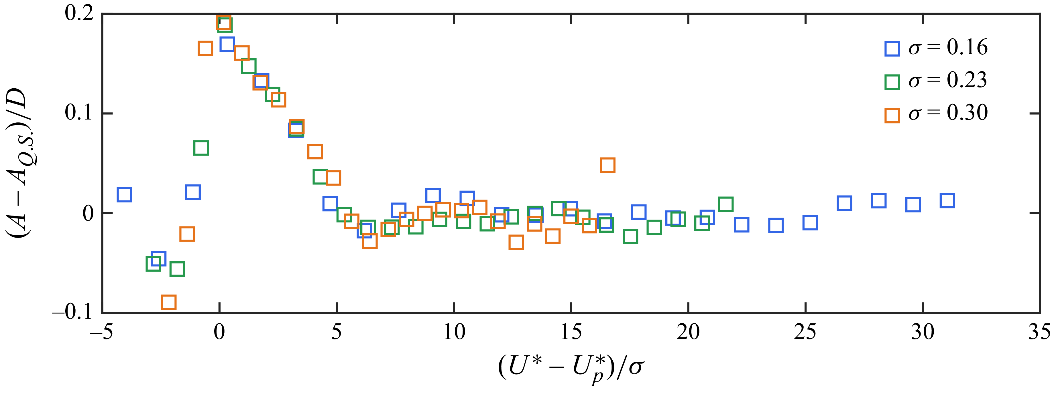


 Open access