


1. Introduction
Surface roughness profoundly impacts turbulent boundary layers. Relative to a smooth surface, roughness increases not only drag but also heat and mass transfer, with consequences for efficiency, emissions and the climate. In international shipping, for example, biofouled-roughened ship hulls increase fuel consumption by tens of billions of dollars annually, along with a proportional increase in greenhouse gas emissions. Yet our ability to manage the consequences is paced by our skill in predicting the drag of rough surfaces, a longstanding problem in fluid mechanics (Raupach, Antonia & Rajagopalan Reference Raupach, Antonia and Rajagopalan1991; Jiménez Reference Jiménez2004; Flack & Schultz Reference Flack and Schultz2010; Chung et al. Reference Chung, Hutchins, Schultz and Flack2021).
Roughness effects cannot be easily generalized. Barnacles on ship hulls do not engender drag in the same way as trees in the atmospheric surface layer. However, the opposite extreme view, that roughness effects cannot be generalized at all, is also unfounded. It has long been appreciated that, everything else being equal, the larger the roughness size, the greater the drag (Nikuradse Reference Nikuradse1933). And, for a given size, the roughness plan density (the ratio of roughness plan area to wall area), plays a key role in determining drag (Schlichting Reference Schlichting1937). This knowledge is subsequently codified in models and frequently refined as new data become available to address model weaknesses (Flack & Chung Reference Flack and Chung2022).
Roughness models are formulas for drag that are fitted to topographical parameters. Topographical parameters only depend on the roughness geometry. In this way, models link drag with roughness features that are likely to matter. For example, the roughness frontal density is important because pressure drag is proportional to the frontal area (Simpson Reference Simpson1973). Skewness captures the observation that peaks are more draggy than valleys (Flack & Schultz Reference Flack and Schultz2010; Jelly & Busse Reference Jelly and Busse2018) and effective slope captures the observation that steeper slopes are more draggy than shallow slopes (Napoli, Armenio & De Marchis Reference Napoli, Armenio and De Marchis2008). As it became clear which sets of these parameters are independent (Placidi & Ganapathisubramani Reference Placidi and Ganapathisubramani2015; Thakkar, Busse & Sandham Reference Thakkar, Busse and Sandham2017), and with ready access to rapid prototyping both in laboratory experiments (computer numerical control machining) and in numerical simulations (immersed boundaries), research shifted to systematic sweeps in parameter space (Schultz, Kavanagh & Swain Reference Schultz, Kavanagh and Swain1999; Chan et al. Reference Chan, MacDonald, Chung, Hutchins and Ooi2015; Forooghi et al. Reference Forooghi, Stroh, Magagnato, Jakirlić and Frohnapfel2017; Barros, Schultz & Flack Reference Barros, Schultz and Flack2018; Kuwata & Kawaguchi Reference Kuwata and Kawaguchi2019; Flack, Schultz & Barros Reference Flack, Schultz and Barros2020; Ma et al. Reference Ma, Xu, Sung and Huang2020; Jouybari et al. Reference Jouybari, Yuan, Brereton and Murillo2021; Jelly et al. Reference Jelly, Ramani, Nugroho, Hutchins and Busse2022; Yang et al. Reference Yang, Stroh, Chung and Forooghi2022). Machine learning tools have now been brought to bear on the rapidly growing dataset. To account for the many types of surfaces, more extensive statistical features (Jouybari et al. Reference Jouybari, Yuan, Brereton and Murillo2021), and even the surface elevation probability density functions and power-spectral densities are taken as input (Yang et al. Reference Yang, Stroh, Lee, Bagheri, Frohnapfel and Forooghi2023; Yousefi et al. Reference Yousefi, Hora, Yang, Veron and Giometto2024). As the roughness parameter space is infinite, with unfamiliar surfaces or unexpected behaviour reported from time to time (Barros et al. Reference Barros, Schultz and Flack2018; Nugroho et al. Reference Nugroho, Monty, Utama, Ganapathisubramani and Hutchins2021; Womack et al. Reference Womack, Volino, Meneveau and Schultz2022; Hutchins et al. Reference Hutchins, Ganapathisubramani, Schultz and Pullin2023), physically interpretable predictions are essential for reliability (Brunton, Noack & Koumoutsakos Reference Brunton, Noack and Koumoutsakos2020), but how to do so is an active area of research.
One approach to physical interpretability is to use topographical parameters motivated by or derived from flow physics. In addition to interpretability, topographical parameters are relatively easy to port, e.g. in a dynamic procedure of a large-eddy simulation (Anderson & Meneveau Reference Anderson and Meneveau2011) or in a neural network. A benefit of interpretability is the underlying physical hypothesis can be tested and advanced. Ideally, only a few parameters and a few fitting constants are used. One enduring parameter is the frontal solidity (Schlichting Reference Schlichting1937; Jiménez Reference Jiménez2004) or closely related parameters such as the effective slope. When roughness features are sparsely spaced, the higher the frontal solidity, the higher the drag. However, when roughness features are densely packed to shelter one another from the oncoming flow, the higher the frontal solidity, the lower the drag. This sheltering effect is described comprehensively by Grimmond & Oke (Reference Grimmond and Oke1999) and encapsulated in the formula of Macdonald, Griffiths & Hall (Reference Macdonald, Griffiths and Hall1998), whose predictive skill was found to be impressive in untested parameter spaces (Chung et al. Reference Chung, Hutchins, Schultz and Flack2021). Sheltering was extended in a series of studies (Yang & Meneveau Reference Yang and Meneveau2016, Reference Yang and Meneveau2017; Yang et al. Reference Yang, Sadique, Mittal and Meneveau2016; Sadique et al. Reference Sadique, Yang, Meneveau and Mittal2017) to directly predict drag from surface elevation maps of tall prisms, fractal and directional surfaces, bypassing the use of topographical parameters. In addition to regular surfaces, sheltering also applies to irregular surfaces (Yang et al. Reference Yang, Stroh, Chung and Forooghi2022) and it turns out that sheltering also plays a decisive role on heat transfer (Abu Rowin et al. Reference Abu Rowin, Zhong, Saurav, Jelly, Hutchins and Chung2024). Although frontal solidity was used and discussed hand in hand with sheltering, by itself the frontal solidity does not encapsulate our current understanding of roughness flow physics. For example, the frontal solidity does not discriminate between the differences in pressure drag due to gentle vs steep roughness slopes. A related point is that the frontal solidity needs to be used with the plan solidity or skewness to differentiate sparse surfaces with occasional spikes from wavy surfaces. Although the link between pressure drag and frontal area is proportional, the addition of plan solidity or skewness is somewhat ad hoc. In addition, frontal solidity, even with the inclusion of skewness or plan solidity, cannot account for clustering, which can alter levels of sheltering of roughness elements (Sarakinos & Busse Reference Sarakinos and Busse2022).
The present effort is focused on a physics-based analysis to determine and propose a geometric parameter, called the wind-shade roughness factor, which by itself has predictive capabilities. In the future, it can also be combined with other parameters and further extend possible machine learning approaches, or, more simply, be used as single parameter. The proposed predictive model based on the wind-shade roughness factor is easily implemented by other researchers, and to further ease of implementation, the code and some example applications are provided as a computational notebook together with this paper. The intended use for the present roughness model is routine calculations based on available elevation maps, reduced to a simple geometric parameter like the skewness or effective slope, without involving complicated solutions to non-local partial differential equations (e.g. solving Laplace's equation) such as the force-partitioning-inspired method (Aghaei-Jouybari et al. Reference Aghaei-Jouybari, Seo, Yuan, Mittal and Meneveau2022) or having to perform fluid dynamics simulations. Moreover, the number of fitting constants required to reproduce data should be much smaller than the number of data points available for validation.
In the present paper, the wind-shade factor can be seen as a geometric parameter that combines both effects of plan and frontal solidities, or skewness and effective slope. Its physical derivation is presented in § 2 while the effects of viscosity for transitional roughness are added in § 3. Predictions and comparisons with data are given in § 4, and the impact of various modelling choices is analysed in § 5. Results for transitionally rough surfaces are considered in § 6. Concluding remarks are provided in § 7.
2. The wind-shade roughness model
We consider a rough surface whose elevation is given by a single-valued function  $h(x,y)$. The first goal is to estimate the form (pressure) drag force arising when this surface is placed in a turbulent flow, under fully rough conditions. For such conditions, the representation should depend only upon the surface geometry, the direction of the flow with respect to that geometry (e.g. an angle $\phi$) and the turbulence spreading angle $\theta$. The overall tangential force per unit mass in the two horizontal directions, $f_x$ and $f_y$, is expressed as an area integral of the pressure-caused kinematic wall stress along the entire surface
 \begin{equation} {f_x} ={-} \iint_A {\tau^p_{xz}}(x,y) \, {{\rm d}\kern0.07em x}\, {{\rm d}y} ={-} \iint_A \frac{1}{\rho} p(x,y) \, \frac{\partial h}{\partial x} \, F^{sh}(x,y;\phi,\theta) \, {{\rm d}\kern0.07emx} \,{{\rm d}y}, \end{equation}
and similarly for  $f_y$ involving the local slope in the $y$ direction, $\partial h/\partial y$. Mathematically speaking, we only require the function $h(x,y)$ to be single valued (e.g. wall-attached cubes would involve Heaviside functions, and delta-Dirac functions for the surface's local slopes which when integrated lead to terms proportional to projected frontal area). In practice, most often the integration is done numerically, for which we assume $h(x,y)$ to be discretized on a fine grid and its gradients determined using (e.g.) finite differencing. The stress $\tau _{xz}^p(x,y)$ is the pressure (form) drag force per unit planform area of the rough surface. The pressure field $p(x,y)$ is relative to some reference pressure $p_\infty =0$. The factor $F^{sh}(x,y;\phi,\theta )$ is the sheltering function described in the next section.
2.1. Sheltering function
The sheltering function  $F^{sh}(x,y;\theta )$ is defined as
 \begin{equation} F^{sh}(x,y;\theta)=H(\theta - \beta(x,y)), \end{equation}
where  $\beta (x,y)$ is the angle made by any given point with its upstream horizon, while $\theta$ is the turbulence spreading angle which will be considered a model parameter. Also, $H(x)$ is the Heaviside function. The sheltering function requires knowledge of the angle $\beta (x,y)$, the angle between the horizontal direction and a point's ‘backward horizon’ point (Dozier, Bruno & Downey Reference Dozier, Bruno and Downey1981). To define the backward horizon function, it is convenient to assume that the $x$ direction is aligned with the incoming velocity $u_i$, i.e. $u_2=0$ (any dependence on $\phi$ omitted henceforth from the notation). The function $x_b(x)$ is called the ‘backward horizon function’ of point $x$ (Dozier et al. Reference Dozier, Bruno and Downey1981) and is the position of the visible horizon looking into the negative direction (or upstream towards the incoming flow) from point $x$. For the maximum of $h(x,y)$, one sets $x_b(x)=x$. Then the horizon angle at point $(x,y)$ is given by
 \begin{equation} \tan \beta = \frac{h(x_b(x),y)-h(x,y)}{x_b(x)-x}. \end{equation}
 Figure 1 shows the various angles for any given position  $x$ as well as the horizon function $x_b(x)$. The angle distribution $\beta (x,y)$ depends only upon the surface geometry via the backward horizon function and need only be determined once for a given surface (i.e. it does not depend upon the turbulence spreading angle $\theta$). The landscape shading literature (e.g. Dozier et al. Reference Dozier, Bruno and Downey1981) includes fast, $O(N)$ (where N is the number of discrete points along x), algorithms to determine the horizon function $x_b(x)$. With these methods, evaluation of the sheltering factor $F^{sh}(x,y;\theta )$ can be done very efficiently for any given $\theta$ since $\beta (x,y)$ can be pre-computed for a given surface.
Sketch of surface, turbulence spreading angle  $\theta$ and backward horizon angle $\beta (x,y)$ for any given point $(x,y)$. Since in the example shown the point $x$ has a backward horizon angle $\beta$ that is larger than the turbulence spreading angle $\theta$, point $x$ is considered sheltered (wind shaded).

As illustration, in figure 2 we show a sample surface (case of turbine-type roughness with transverse ( $y$-aligned) ridges from Jelly et al. Reference Jelly, Ramani, Nugroho, Hutchins and Busse2022) for two angles: $\theta =5^\circ$ (a) and $\theta =15^\circ$ (b). Black regions are shaded regions. The drag (and hence the effective hydrodynamic roughness height for case (b) is expected to be larger due to more frontal area being exposed to the flow.
Surface and its shaded regions for two angles  $\theta =5^{\circ }$ (a) and $\theta =15^{\circ }$ (b). Computation of shaded region is based on the fast algorithm of Dozier et al. (Reference Dozier, Bruno and Downey1981), separately for each $x$-line in the direction of the incoming flow velocity $u_1$. In this and all subsequent elevation map visualizations, in order to represent the appropriate relative dimensions and surface slopes, the axes are normalized by a single scale $L_y$, the width of the domain, i.e. $x_s=x/L_y$, $y_s=y/L_y$ and $h_s=h/L_y$. The surface height is indicated by colours, ranging from light yellow to dark purple from highest to lowest elevation of each surface, respectively. Wind-shaded portions of the surface are indicated in black.

2.2. Modelled pressure distribution
To determine the pressure distribution  $p(x,y)$, it is useful to select a reference velocity. We chose a notional velocity denoted by $U_k$ representing the velocity at a height $z_k$ above the mean surface elevation (note that the index $k$ here refers to roughness height, often denoted by the letter $k$, and is not meant as a vector element index). The height $z_k$ is assumed to be sufficiently large so that the time-averaged mean velocity there can be assumed to be independent of $(x,y)$. We thus aim for a height just above the roughness sublayer where assuming that the time-averaged streamwise velocity is constant over $(x,y)$ is appropriate.
We now turn to the pressure (form) drag model. We use the piecewise potential ramp flow approach (Ayala et al. Reference Ayala, Sadek, Ferčák, Cal, Gayme and Meneveau2024) (see figure 3) to model  $p(x,y)$. We simplify any sloping portion of a roughness element or portions of a surface as a planar ramp inclined at an angle $\alpha$. The ramp angle is obtained from $\alpha = \arctan |\boldsymbol {\nabla }_h h|$ (i.e. based on the absolute value of the surface slope, for reasons to be explained below), and $\boldsymbol {\nabla }_h$ is the gradient in the horizontal plane, $\boldsymbol {\nabla }_h=\partial _x {\boldsymbol {i}}+\partial _y\kern0.09em {\boldsymbol {j}}$. We assume at the bottom of each ramp flow, there is a stagnation point (solid circle in figure 3b) and at the top of the ramp the velocity is $U_k$ and the pressure there is equal to the reference pressure $p_\infty =0$, i.e. we assume plug flow between height $z_k$ and the ramp top. Evidently, this is a strong assumption but is necessary if we wish to apply a potential flow description that is purely ‘local’, i.e. is agnostic of flow conditions at other locations and far above the surface.
Sketch of surface discretized at horizontal resolution  $\Delta x$ and (b) potential flow over a ramp at angle $\alpha$ (Ayala et al. Reference Ayala, Sadek, Ferčák, Cal, Gayme and Meneveau2024) assumed to be locally valid over the surface at horizontal discretization length $\Delta x$. In (a,b) the surface slope is assumed to be only in the $x$ direction, i.e. $\hat {n}_x=1$. The lowest point of the ramp has a stagnation point while at the end point the velocity magnitude is assumed to be $U_{ref}$ and pressure is $p_\infty =0$. (c) Shows a sketch of isosurface contours (surface seen from above), the local normal vector $\hat {\boldsymbol {n}} = \boldsymbol {\nabla }_h h/|\boldsymbol {\nabla }_h h|$, the incoming velocity $U_k$ in the $x$ direction and the incoming velocity normal to the surface becomes $U_{ref} = U_k \hat {n}_x$.

Following the development in Ayala et al. (Reference Ayala, Sadek, Ferčák, Cal, Gayme and Meneveau2024), we use the known solution for potential flow over a ramp, for which the streamfunction in polar coordinates is given by  $\psi (r,\theta ) = B r^n \sin [n(\theta -\alpha )]$, with $n={\rm \pi} /({\rm \pi} -\alpha )$ and $B$ is the streamfunction amplitude to be expressed later as a function of the local velocity magnitude. The radial coordinate runs from $r=0$ at the stagnation point to $r={\ell }_r$ at the top of the ramp, where the velocity is a known reference velocity $U_{ref}$ and the pressure is $p_\infty =0$. The radial (tangential to the surface) velocity component along the ramp surface is $V_r=-(1/r)\partial \psi /\partial \theta$ evaluated at $\theta =\alpha$. It results in $V_r(r) = n B \, (r/\ell _r)^{n-1}$, which can be seen to fix $n B = U_{ref}$. Using the Bernoulli equation to evaluate the pressure difference between points at the crest and along the surface yields
 \begin{equation} \frac{1}{\rho} \, p(r) = \frac{1}{2} U_{ref}^2 \left[ 1 - \left(\frac{r}{\ell_r}\right)^{2\alpha/({\rm \pi}-\alpha)}\right]. \end{equation}
Only the horizontal velocity normal to the surface is expected to generate a pressure differential, i.e. the reference velocity  $U_{ref}$ would vanish if the surface does not present a component standing normal to the incoming flow direction. This effect can be taken into account by setting $U_{ref} = U_k \hat {n}_x$, where
 \begin{equation} \hat{n}_x = \frac{\partial h/\partial x}{|\boldsymbol{\nabla}_h h|}, \end{equation}
is based on the horizontal gradient of the elevation map  $h(x,y)$. For a surface that is inclined normal to the incoming flow, e.g. front faces of wall-attached cubes, $\hat {n}_x=1$ and thus $U_{ref} = U_k$. On the side faces of such cubes, $\hat {n}_x$ and $U_{ref}$ vanish, as the flow skims past such surfaces with no pressure buildup from the potential flow ramp model (see figure 3c).
Next, we compute the mean pressure on the ramp segment,  $\bar {p}={\ell _r}^{-1}\int _{r=0}^{\ell _r} p(r) \, {\rm d}r$, which results in
 \begin{equation} \frac{1}{\rho} \, \bar{p}(x,y) = (U_k \hat{n}_x)^2 \,\frac{\alpha(x,y)}{{\rm \pi}+\alpha(x,y)}. \end{equation}
To obtain the pressure force in the  $x$ direction, i.e. in order to derive the form provided in (2.1), we multiply by the projected surface area vector $|\boldsymbol {\nabla }_h h| \hat {n}_x \Delta x \Delta y$, where $\Delta x$ and $\Delta y$ are the horizontal spatial resolutions describing the surface (and the length $\ell _r$ used to evaluate the mean pressure is $\ell _r \sim (\Delta x \Delta y)^{1/2}$). Including the shading function, the resulting local kinematic wall stress in the $x$-direction coming from pressure (i.e. dividing the pressure force by the planform area $\Delta x \Delta y$ and density) can be written as
 \begin{equation} \tau_{xz}^{p} = (U_k \, \hat n_x)^2 \, \frac{\alpha}{{\rm \pi}+\alpha} \,\frac{\partial h}{\partial x}\, F^{sh}. \end{equation}
For small slopes, we have  $\alpha \approx |\boldsymbol {\nabla }_h h| \ll {\rm \pi}$, and then the pressure drag is quadratic with slope (as is known to be the case for small-amplitude waves Jeffreys Reference Jeffreys1925). However, for present applications, in which for certain types of surfaces the local slopes could go up to ${\rm \pi} /2$ (vertical segments, although with finite resolution discretely representing $h(x,y)$, some small deviations from vertical are unavoidable), we do not use nor need this small angle approximation.
Now, instead of following Ayala et al. (Reference Ayala, Sadek, Ferčák, Cal, Gayme and Meneveau2024) in which only the windward facing portion of the surface feels a pressure force (the leeside portion was assumed to exhibit either flow separation or incipient separation such that the pressure force there was neglected), we here allow for pressure recovery for downward facing portions of the surface. To model the absence of pressure recovery in separated or nearly separated region we here rely entirely on the sheltering function  $F^{sh}(x,y;\theta )$ treated in subsection 2.1. Without flow separation, the potential flow ramp model predicts a flow along a downward ramp with the stagnation pressure at the bottom of the ramp and a resulting force in the negative $x$ direction, i.e. pressure recovery. The sign of the resulting force is given by the surface slope in the $x$-direction ( $\partial h/\partial x$) but the magnitude is the same independent of flow direction (for inviscid flow). By choosing to define the angle $\alpha$ using an absolute value of the ramp slope and use $\partial h/\partial x$ to determine the direction of force, we enable pressure recovery on backward sloping parts of the surface that are not in the sheltered portions of the surface (for surfaces to be studied in this work, however, this effect appears to be of negligible importance).
2.3. Wind-shade factor
Combining the sheltering and inviscid pressure models, we write the total (kinematic) force for a flow in the  $x$ direction ( $i=1$) as
 \begin{equation} f_x = u_\tau^2 A = U_k^2 \, \iint_A \hat n_x^2 \, \frac{\alpha}{{\rm \pi}+\alpha} \, \frac{\partial h}{\partial x} \, F^{sh}(x,y;\theta) \, {{\rm d}\kern0.07em x} \,{{\rm d}y}, \end{equation}
and the averaging is performed over the entire surface, i.e. over all  $(x,y)$. This expression can be solved for the velocity $U_k$ normalized by friction velocity $u_\tau$ as follows:
 \begin{equation} U_k^+= \frac{1}{\sqrt{ {\mathcal{W}}_{L}} }, \end{equation}
where it is useful to define the streamwise (longitudinal, ‘L’) wind-shade factor  ${\mathcal {W}}_{L}$ using a surface average
 \begin{equation} {\mathcal{W}}_{L} = \left\langle \hat n_x^2(x,y) \,\frac{\alpha}{{\rm \pi}+\alpha} \, \frac{\partial h}{\partial x} \, F^{sh}(x,y;\theta) \right\rangle_{x,y},\quad{\rm where}\ \alpha(x,y) = \arctan|\boldsymbol{\nabla}_h h(x,y)| . \end{equation}
The averaging operation is meant to indicate the surface integral as in (2.8) divided by plan area  $A$. It is important to note that, owing to the fact that potential flow is purely dependent on surface geometry, the wind-shade factor ${\mathcal {W}}_{L}$ is also a purely geometric quantity depending only on the surface height distribution, the mean flow direction relative to the surface and the assumed turbulence angle $\theta$.
For future reference, we point out that, for certain surfaces with directional preference (e.g. inclined ridge-like features), one can also define a transverse wind-shade factor  ${\mathcal {W}}_T$ according to
 \begin{equation} {\mathcal{W}}_{T} = \left\langle \hat n_x ^2 \, \frac{\alpha}{{\rm \pi}+\alpha} \, \frac{\partial h}{\partial y} \, F^{sh}(x,y;\theta) \right\rangle_{x,y} . \end{equation}
It involves the pressure force built up due to streamwise velocity but projected onto the transverse direction as a result of the local slope  $\partial h/\partial y$. This transverse factor represents the surface-induced drag force in a direction perpendicular to the incoming flow due to anisotropy of the surface topography.
2.4. Reference height
In order to relate the estimated drag force and wind-shade factor to roughness ( $z_0$) or equivalent sandgrain ( $k_s$) roughness lengths, we must choose an appropriate height to evaluate the log law. The common wisdom is that the roughness sublayer extends to approximately 2–3 times the representative heights of roughness elements, (Jiménez Reference Jiménez2004; Flack, Schultz & Connelly Reference Flack, Schultz and Connelly2007), although further dependencies on in-plane roughness length scales are also known to affect the height of the sublayer (Raupach, Thom & Edwards Reference Raupach, Thom and Edwards1980; Meyers, Ganapathisubramani & Cal Reference Meyers, Ganapathisubramani and Cal2019; Sharma & García-Mayoral Reference Sharma and García-Mayoral2020; Endrikat et al. Reference Endrikat, Newton, Modesti, García-Mayoral, Hutchins and Chung2022). For general surfaces, the height of roughness elements is difficult to specify and a more general definition for arbitrary functions $h(x,y)$ must be devised. Using the mean elevation $\bar {k} = \langle h \rangle$ as the baseline height, we define a dominant positive height $k_{p}^\prime$ according to
 \begin{equation} \left.\begin{gathered} k_{p}^\prime = \langle [R(h^\prime)]^p\rangle^{1/p},\quad{\rm where}\ h^\prime = h-\langle h\rangle,\\ {\rm and}\\ R(z)=z\quad {\rm if}\ z \geqslant 0,\quad R(z)=0\quad {\rm if}\ z < 0, \end{gathered}\right\} \end{equation}
is the ramp function. As  $p \to \infty$, the scale $k_{p}^\prime$ tends to the maximum positive deviation above the mean height over the entire surface. A choice of $p=8$ turns out to be sufficiently high to both emphasize the highest points but still include weak contributions from the entire surface for statistical robustness, for practical applications.
As the reference height where we evaluate the log law and where we assume the reference velocity  $U_k$ is constant (i.e. the mean velocity only depends on $z$ and not on $(x,y)$), we select a height $\bar {k}+a_p k_{p}^\prime$, with $a_p=3$, a choice motivated by the observations that the roughness sublayer extends to approximately 3 times the characteristic element heights. Since $a_p$ is somewhat arbitrarily chosen, we can regard this parameter as an adjustable one, but as a first approximation the choice $a_p=3$ appears reasonable. The sketch in figure 4 illustrates three types of surfaces and the resulting reference heights given the maximal positive height fluctuation away from the mean.
Sketch of surfaces with height distribution  $h(x,y)$ and near zero (a), positive (b) and negative (c) skewness. Also shown are the mean height $\bar {k}$, the dominant positive height $k_{p}^\prime$ and the resulting reference height $a_p k_{p}^\prime$ (with $a_p \sim 3$ to be used in the model) above the mean height.

With these assumptions, equivalent roughness scales  $z_{0}$ and sandgrain-roughness heights $k_s$ can be obtained as usual (Jiménez Reference Jiménez2004) from $U_k^+ = (1/\kappa ) \ln (z_k/z_0) = (1/\kappa ) \ln (z_k/k_s) + 8.5$, with $z_k=a_p k_{p}^\prime$, and hence
 \begin{equation} z_{0} = a_p \, k_{p}^\prime \exp\left(-\kappa U_k^+ \right), \end{equation}
and similarly for  $k_s$. Additionally, an overall reference scale for surface height will be chosen as $k_{rms} = \langle (h-\bar {k})^2\rangle ^{1/2}$, the root mean square (r.m.s.) of the surface height function $h(x,y)$ over all $(x,y)$. This choice facilitates comparison with datasets for which $k_{rms}$ is often prescribed and known.
Finally the wind-shade model for sandgrain-roughness normalized by r.m.s. height is given by
 \begin{equation} \frac{k_{s-mod}}{k_{rms}} = a_p \, \frac{k_p^\prime}{k_{rms}} \exp\left[-\kappa (U_k^+- 8.5) \right], \end{equation}
with  $U_k^+ = {\mathcal {W}}_L^{-1/2}$ for the case of fully rough conditions (see § 3 below for transitionally rough cases). It is important to point out that we are not assuming that, physically, the height $z_k=a_p k_p^\prime$ falls in the logarithmic layer, but are using (2.13) or (2.14) as a definition of $k_s$ or $z_0$: For a given velocity $U_k$ at height $z_k$, what is the length scale $k_s$ or $z_0$ that, when entered into the simple log law, will predict the correct friction velocity or stress?
2.5. Turbulence spreading angle
The angle  $\theta$ describing the effect of turbulent mixing at the reference height determines the strength of the sheltering effect. If the angle is large, the sheltering region will decrease rapidly in size and increase drag due to larger exposed downstream roughness features (see figure 2). Conversely, for smoothly rounded surfaces, increasing $\theta$ will lead to delayed separation on the back sides of rounded roughness elements and hence to partial pressure recovery, which would decrease the drag.
For the default model, we assume a constant angle and chose  $10^\circ$ as representative of values expected from the literature (e.g. Abu Rowin et al. Reference Abu Rowin, Zhong, Saurav, Jelly, Hutchins and Chung2024). Another option, as proposed in Yang et al. (Reference Yang, Sadique, Mittal and Meneveau2016), is to assume that the turbulence spreading angle $\theta$ is proportional the ratio of vertical r.m.s. turbulence velocity (which is of same order as $u_\tau$) and the streamwise advection velocity $U_k$ at the reference height, i.e.
 \begin{equation} \tan \theta = \frac{u_\tau}{U_k}=\frac{1}{U_k^+} = {\mathcal{W}}_{L}^{1/2}. \end{equation}
The wind-shade factor and the angle must then be determined iteratively. (Equation (2.15) is meant for cases when  ${\mathcal {W}}_T=0$, since otherwise the friction velocity $u_\tau$ would also be expected to depend on ${\mathcal {W}}_T$.)
2.6. Near-wall velocity profile
A further refinement relates to the assumed velocity near the roughness elements. The definition of the wind-shade factor  ${\mathcal {W}}_{L}$ relies on the assumption that the velocity is constant (plug flow) from $z_k$ down to near the crest of any of the surface features or roughness elements. For surfaces with a few large-scale elements and many very small-scale elements (e.g. multiscale roughness), this may lead to a drag over-prediction caused by the small-scale elements that in reality might be exposed to a smaller velocity there. A possible remedy is to assume a 1/7 velocity power-law profile impinging on the roughness elements of the form $U(z) = U_k [(h(x,y)-h_{min})/(h_{max}-h_{min})]^{1/7}$. In this case, the definition of the wind-shade factor becomes
 \begin{equation} {\mathcal{W}}_{L,vel} = \left\langle \left(\frac{h(x,y)-h_{min}}{h_{max}-h_{min}}\right)^{2/7}\, \hat{n}_x^2(x,y) \, \frac{\alpha}{{\rm \pi}+\alpha} \, \frac{\partial h}{\partial x} \, F^{sh}(x,y;\theta) \right\rangle_{x,y}. \end{equation}
The introduction of a factor that decreases to zero near the minimum of the surface may improve the predictive power of the wind-shade factor. Note that this expression is still purely dependent on the surface geometry, although as with the pressure distribution model, it is fluid mechanics inspired.
At this stage, it is useful also to comment on connections to existing parameters. For instance, for vertical surfaces with  $\alpha ={\rm \pi} /2$, the slope correction term $\alpha /({\rm \pi} + \alpha ) = 1/3$, and the flow-direction correction is $\hat {n}_x^2 = 1$, and if the wind shading $F^{sh} = 1$ if $\partial h/\partial x > 0$ and $0$ otherwise, then we recover one third of the frontal solidity as the model's prediction. In terms of the formula of Macdonald et al. (Reference Macdonald, Griffiths and Hall1998) that accounts for densely packed roughness features, choosing as wind shading $F^{sh} = 1$ for sparse roughness and $F^{sh} = 0$ for dense roughness is similar to the damping factor introduced that is also $1$ and $0$ as the plan solidity varies between $0$ and $1$, respectively. However, in the present model, $F^{sh}$ is linked in more detail with the underlying flow physics given its detailed $(x,y)$ dependence that can also be locally correlated to the value of $\alpha (x,y)$. The inclusion of the slope correction $\alpha /({\rm \pi} +\alpha )$ is expected to discriminate between spiky vs undulating surfaces, an argument usually given to include the surface skewness as relevant parameter. Moreover, directional and clustering effects are all naturally accounted for.
3. Effects of viscosity: transitionally rough flows
Since in many cases viscous effects are expected to be important (transitionally rough cases), we now include the contributions from viscous stresses. Following Raupach (Reference Raupach1992), we model the local kinematic viscous stress as a function of the assumed velocity  $U_k$ using a friction factor
 \begin{equation} {\tau^{\nu}_{xz}} = \tfrac{1}{2} \, c_f(Re_k) \, U^2_k. \end{equation}
The smooth-surface friction factor  $c_f$ can be written in terms of a Reynolds number $Re_k=z_k U_k/\nu$ based on the height $z_k=a_p k_p^\prime$ and velocity there, $U_k$. The viscous stress $\tau ^{\nu }_{xz}$ acts in the unsheltered regions. To include the sheltering we multiply by the average of the sheltering function $\langle F^{sh}\rangle$. However, for transitionally and hydrodynamically smooth surfaces the sheltering effect decreases and must entirely vanish in the limit of a smooth surface, regardless of the existence of geometric roughness. For hydrodynamically smooth cases, the flow around geometric roughness elements becomes essentially low Reynolds number (tending to Stokes flow), with more and more attached flow and no sheltering. Hence, we introduce the average viscous sheltering factor
 \begin{equation} \bar{F}_\nu^{sh}(z_k^+) = \langle F^{sh}\rangle + (1- \langle F^{sh}\rangle ) \left[1+\left( {z_k^+}/{10}\right)^2 \right]^{{-}1/2}, \end{equation}
which switches from the rough limit  $\bar {F}_\nu ^{sh} = \langle F^{sh}\rangle$ (expected when $z_k^+ \gg 10$) to $\bar {F}_\nu ^{sh} =1$ when approaching hydrodynamically smooth-surface behaviour (expected when $z_k^+ \ll 10$). Strictly speaking, we should make a similar adjustment to the wind shade factor ${\mathcal {W}}_{L}$, since in the limit of transitionally and hydrodynamically smooth surfaces one would expect an absence of flow separation, and therefore full pressure recovery, over the backward facing surfaces. However, one would then need to transition to a low Reynolds number model for pressure, instead of the quadratic inviscid model used for defining ${\mathcal {W}}_{L}$. In practice, since the viscous $c_f$ term dominates at low $Re_k$, such an adjustment would have very little impact on results, and in the interests of simplicity such adjustments are omitted, and the definition of ${\mathcal {W}}_{L}$ based on a purely inviscid quadratic drag law is retained.
The total drag force can then be written as
 \begin{equation} f_x = u_\tau^2 A = U_k^2 \,{\mathcal{W}}_{L} A + U_k^2 \tfrac{1}{2} \, c_f(Re_k) \,\bar{F}_\nu^{sh}(z_k^+) A, \end{equation}
or, solving again for  $U_k^+$,
 \begin{equation} U_k^+= \left[{\mathcal{W}}_{L} + \tfrac{1}{2} \, c_f(Re_k) \bar{F}_\nu^{sh}(z_k^+) \right]^{{-}1/2} ,\end{equation}
since  $U_k$ (and thus $Re_k$) is assumed to be the same over entire surface. We also recall that $Re_k = U_k z_k/\nu = U_k^+ z_k^+ = U_k^+ (z_k /k_{rms}) k_{rms}^+$ with $z_k=a_p k_p^\prime$, which for a prescribed value of $k_{rms}^+$ and known geometric ratio $(a_p k_p^\prime /k_{rms})$ enables us to determine the Reynolds number in terms of $U_k^+$.
Next, the friction factor must be determined. We use the generalized Moody diagram fit (Meneveau Reference Meneveau2020), appropriately rewritten in its simplest form according to
 \begin{equation} c_f(Re_k) = 0.0288 \, Re_k^{{-}1/5} \left(1+577 Re_k^{{-}6/5}\right)^{2/3}. \end{equation}
This is a fit to the numerical solution of the one-dimensional equilibrium fully developed (parallel flow) wall-bounded flow problem. It represents a generalization of the Moody diagram method relating wall stress to bulk velocity but here used only for the smooth line of the Moody diagram, or the skin-friction law for a smooth wall, where  ${Re}_k$ replaces the outer Reynolds number. Also, the input parameter ${Re}_k$ is expressed at some reference height $z_k^+$ that may fall in the logarithmic or viscous sublayer, instead of an outer-layer height as is usual for the Moody diagram. For more details, see Meneveau (Reference Meneveau2020). Thus, in the limit of small Reynolds number (i.e. when $z_k^+ \sim 1$, and the velocity profile up to maximal height is linear), the limiting behaviour is $c_f \to 2/Re_k$ and $\bar {F}_\nu ^{sh}(z_k^+)\to 1$. For $k \sim x^{1/2}$, this trend is similar to Blasius. For increasing Reynolds number, the friction factor fitting function goes to a $Re_k^{1/5}$ high Reynolds number behaviour.
To solve (3.4) we can employ numerical iteration. Since the weakest dependence is on the  $c_f$ function, it is convenient to simply iterate the rapidly converging expression
 \begin{equation} {U_k^+}^{(n+1)} = \left( {\mathcal{W}}_{L} + \tfrac{1}{2} c_f( {U_k^+}^{(n)} z_k^+ ) \,\bar{F}_\nu^{sh} \right)^{{-}1/2}, \end{equation}
always recalling that  $z_k^+ = (a_p k_p^\prime /k_{rms}) k_{rms}^+$, and starting with some initial guess (e.g. near frictionless $c_f^{(n=0)}=10^{-14}$). Once $U_k^+$ has been determined, the equivalent sandgrain roughness $k_s$ is again determined via (2.14).
4. Results
4.1. Suite of surfaces from roughness database and others
In this section we apply the wind-shade roughness model to over 100 surfaces for which the full height distribution  $h(x,y)$ is known and the equivalent sandgrain roughness $k_s$ has been measured. Appendix A lists the datasets considered (most of the surfaces are obtained from a public database at https://roughnessdatabase.org). Summarizing, they include 3 rough turbine blade-type surfaces from Jelly et al. (Reference Jelly, Ramani, Nugroho, Hutchins and Busse2022) (isotropic and with dominant streamwise or spanwise aligned ridges), 26 cases studied numerically by Jouybari et al. (Reference Jouybari, Yuan, Brereton and Murillo2021) including several types of sandgrain bumps, regular bumps, sinusoidal surfaces and one wall-attached cube case, 7 cases of rough surfaces studied experimentally in Flack et al. (Reference Flack, Schultz and Barros2020), truncated cones in random arrangements and along regular staggered arrays, each in 8 different densities studied experimentally in Womack et al. (Reference Womack, Volino, Meneveau and Schultz2022). Also included are 3 eggbox sinusoidal surfaces from the numerical study of Abu Rowin et al. (Reference Abu Rowin, Zhong, Saurav, Jelly, Hutchins and Chung2024), a large collection of 31 surfaces from Forooghi et al. (Reference Forooghi, Stroh, Magagnato, Jakirlić and Frohnapfel2017) studied numerically, 3 power-law surfaces with spectral exponents $-1.5$, $-1$ and $-0.5$ studied experimentally by Barros et al. (Reference Barros, Schultz and Flack2018), surfaces with closely packed cubes with 7 different densities from Xu et al. (Reference Xu, Altland, Yang and Kunz2021) and, finally, 4 cases of multiscale block surfaces studied experimentally by Medjnoun et al. (Reference Medjnoun, Rodriguez-Lopez, Ferreira, Griffiths, Meyers and Ganapathisubramani2021) with up to 3 generations. For a subset of 12 of these surfaces, the panels in figure 5 show the surface elevation and sheltered regions shown as black shadows.
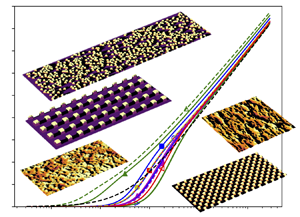
Representative sample of 12 (out of 104) surfaces considered in this study. Black regions are sheltered regions for  $\theta =10^\circ$. Details about the surfaces are provided in Appendix A. Surfaces shown are from (a) Jelly et al. (Reference Jelly, Ramani, Nugroho, Hutchins and Busse2022), $y$-aligned ridges; from Jouybari et al. (Reference Jouybari, Yuan, Brereton and Murillo2021): (b) case C19 (random ellipsoids), (c) case C29 (sinusoidal), (d) and case C45 (wall-attached cubes); (e) from Flack et al. (Reference Flack, Schultz and Barros2020): rough-surface case 1 (specifically, panel 1 from case 1); ( f) from Womack et al. (Reference Womack, Volino, Meneveau and Schultz2022) truncated cones, random case R48, and (g) regular staggered case S57; (h) from Abu Rowin et al. (Reference Abu Rowin, Zhong, Saurav, Jelly, Hutchins and Chung2024) intermediate eggbox (case 0p018); (i) from Forooghi et al. (Reference Forooghi, Stroh, Magagnato, Jakirlić and Frohnapfel2017) case A7060 and (j) case C7088; (k) from Barros et al. (Reference Barros, Schultz and Flack2018) power-law random surface with spectral exponent p=-0.5; and (l) 3-generation multiscale block surface by Medjnoun et al. (Reference Medjnoun, Rodriguez-Lopez, Ferreira, Griffiths, Meyers and Ganapathisubramani2021), case iter 123. The surface height is indicated by colours, ranging from light yellow to dark purple from highest to lowest elevation of each surface, respectively. Shaded portions of the surface are indicated in black.

For each of the 104 surfaces, we first compute the wind-shade factor  ${\mathcal {W}}_{L}$ according to its definition in (2.10). We use the turbulence spreading angle $\theta = 10^\circ$. Then, with the known experimental conditions for each surface expressed as the known $k_{rms}^+$, we determine the effects of viscosity by finding $U_k^+$ according to (3.6). The predicted roughness scale follows from (2.14) using $a_p=3$. The results are shown in figure 6 as scatter plots of predicted/modelled ( $k_{s-mod}$) vs measured ( $k_{s-data}$) sandgrain-roughness scale, each normalized by $k_{rms}$. The correlation coefficient is approximately 77 %. It is also useful to compare the average logarithmic error magnitude, i.e. $e=\langle | \log _{10}(k_{s-mod}/k_{s-data})|\rangle$. The mean error is $e=0.16$ for the wind-shade model. The level of agreement between modelled and measured roughness scale over a large range of surface classes is encouraging.
Sandgrain roughness predicted by the model with  $\theta =10^\circ$ and $a_p=3$, vs measured $k_s$ values from data, for all 104 surface cases considered in this work. Data from Jelly et al. (Reference Jelly, Ramani, Nugroho, Hutchins and Busse2022) (red solid squares), 26 cases from Jouybari et al. (Reference Jouybari, Yuan, Brereton and Murillo2021) (blue solid circles), wall-attached cubes from Jouybari et al. (Reference Jouybari, Yuan, Brereton and Murillo2021) (blue solid square), rough surfaces from Flack et al. (Reference Flack, Schultz and Barros2020) (7 cases, green solid triangles), truncated cones from Womack et al. (Reference Womack, Volino, Meneveau and Schultz2022) (random: maroon triangles, staggered regular: maroon squares), 3 eggbox sinusoidal surface from Abu Rowin et al. (Reference Abu Rowin, Zhong, Saurav, Jelly, Hutchins and Chung2024) (yellow full circles), 31 cases from Forooghi et al. (Reference Forooghi, Stroh, Magagnato, Jakirlić and Frohnapfel2017) (blue sideways open triangles), 3 power-law surfaces with exponent $-1.5$, $-1$ and $-0.5$ from Barros et al. (Reference Barros, Schultz and Flack2018) (green open triangles), surface with 7 cases of closely packed cubes (closed sideways red triangles) from Xu et al. (Reference Xu, Altland, Yang and Kunz2021) and 4 cases of multiscale blocks (open sideways red triangles) from Medjnoun et al. (Reference Medjnoun, Rodriguez-Lopez, Ferreira, Griffiths, Meyers and Ganapathisubramani2021). Panel (a) shows the results in linear units, while panel (b) shows the ratio of modelled to measured sandgrain roughness in logarithmic units.

For comparison with other common roughness models derived from particular datasets, in figure 7(a) we show predictions using the correlations as listed in Flack & Chung (Reference Flack and Chung2022) from Flack et al. (Reference Flack, Schultz and Barros2020) and from Forooghi et al. (Reference Forooghi, Stroh, Magagnato, Jakirlić and Frohnapfel2017), referred to as  $k_{s-Fla}$ and $k_{s-For}$, respectively. These models are implemented here as follows:
 \begin{gather} k_{s-Fla} = k_{rms} \left\{\begin{array}{@{}ll@{}} 2.48 [1+({\min}(1.5,S_k))]^{2.24} & S_k > 0\\ 2.11 & S_k = 0 \\ 2.73 [2+({\max}({-}0.7,S_k))]^{{-}0.45} & S_k < 0 \end{array} \right. \end{gather}
 \begin{gather} k_{s-For} = k_t \,1.07[1-\exp({-}3.5\, ES_x )](0.67 S_k^2+0.93 S_k+1.3), \end{gather}
where the first includes clipping of the skewness factor  $S_k$ into the domain of validity of the fit, $ES_x=\langle |\partial h/\partial x| \rangle$ is the average slope magnitude and $k_t$ is the samples’ peak-to-trough scale, defined as $k_t={\max }(h)-{\min }(h)$. (This definition differs slightly from that used by Forooghi et al. (Reference Forooghi, Stroh, Magagnato, Jakirlić and Frohnapfel2017) – the latter included subdivision of the surface into parts whose extent is specified based on additional parameters – but for present comparative purposes the effects on qualitative trends are relatively small.) Over the 104 surfaces considered here, and including the arbitrary truncation mentioned above, the correlation coefficients between measured and modelled sandgrain-roughness lengths are 36 % and 34 %, respectively, for these two models. The mean logarithmic errors are $e=0.28$ and $e=0.24$, respectively. We have verified that, as expected, when restricting to data for which these correlations were originally developed and fitted by their authors, the correlation is significantly higher and the error lower (see solid symbols in figure 7a).
(a) Sandgrain roughness predicted by the empirical fits of Flack et al. (Reference Flack, Schultz and Barros2020) with truncated skewness (in green), and Forooghi et al. (Reference Forooghi, Stroh, Magagnato, Jakirlić and Frohnapfel2017) (in blue) vs measured values for all 104 surface cases considered in this work. Values used from the respective authors to fit the models are shown as solid symbols. (b) Sandgrain roughness predicted by the model without local pressure term, with  $\theta =10^\circ$ and $a_p=7.5$ vs measured values for all 104 surfaces. Data and symbols same as in figure 6.

Many other correlation and data-based models have been proposed (see review and summary in Flack & Chung Reference Flack and Chung2022) but performing an exhaustive comparison with all of them is beyond the scope of this paper. In addition, the various data-driven and machine learning approaches that have been proposed, while promising in principle, are more challenging to reproduce by others compared with simple function evaluations looped over the surface (as is required in the present approach to compute the wind-shade factor). The main contention of the present work is that our results show that a single geometric parameter  ${\mathcal {W}}_{L}$ can be developed, and that inclusion of such a parameter (e.g. in any other correlations-based or machine-learning-based models) is beneficial, since by itself, with only two adjustable parameters ( $a_p$ and $\theta$), it already provides strong predictive power.
5. Analysis of model terms
In this section, we explore the effects of various included physical effects and model parameters. The effect of selecting  $a_p=3$ is immediately obvious since it only serves as a multiplying factor, leaving the correlation coefficient intact. However, selecting larger or lower $a_p$ (e.g. $a_p=3.5$ or $a_p=2.5$) leads to a cloud falling further above (or below) the line in figure 6 and slightly increases the error parameter $e$. An error fitting procedure shows that the minimum error is indeed obtained for $a_p=3.06$ but the error is almost unchanged. We conclude that selecting $a_p=3$ appears to be a good choice.
Other model ingredients included the potential flow pressure distribution, i.e. selecting a local value of  $\alpha (x,y)/[{\rm \pi} +\alpha {(x,y)}]$ inside the integral, using the projection of the square velocity via the term $\hat {n}_x^2(x,y)$, and including the shading factor $F^{sh}(x,y;\theta)$. The effect of viscous contributions can also be ascertained. Finally, a specified angle $\theta$ was chosen for the model. The effect of each of these choices is analysed next and a summary of the resulting correlation and error coefficients are provided in tabular form (see table 1).
Summary of correlation coefficients and mean logarithmic error between model predicted and measured sandgrain roughness for various versions of the model.

5.1. Potential flow pressure distribution
To quantify the effect of the pressure distribution term, we here define a wind-shade factor using the overall mean pressure as prefactor instead of the local one and do not include the projection normal to the surface (i.e. we also omit the  $\hat {n}_x^2$ term). We define
 \begin{equation} {\mathcal{W}}^{no \, p}_{L} = \left\langle\frac{\alpha}{{\rm \pi}+\alpha} \right\rangle \left\langle \frac{\partial h}{\partial x} \, F^{sh}(x,y;\theta) \right\rangle . \end{equation}
Everything else is left unchanged and the sandgrain roughness is computed using (2.14) but using  ${\mathcal {W}}^{no \, p}_{L}$ instead of ${\mathcal {W}}_{L}$. The ‘best’ value of $a_p$ is obtained by minimizing the error and the resulting value $a_p=7.5$ is used. The scatter plot of predicted sandgrain-roughness scales is shown in figure 7(b). As can be seen, there is visibly much more scatter and the prediction has been severely degraded, with a significantly lower correlation coefficient of $\rho =0.52$ and larger error of $e=0.362$. We conclude that the physics introduced by considering the local pressure acting on surface segments at various angles $\alpha$ provides significant increased predictive power for roughness length estimation.
5.2. Effect of normal velocity projection
We here examine the effect of the projection of the incoming velocity  $U_k$ onto the direction normal to the surface given by the unit vector $\hat {\boldsymbol {n}}$ and its x-direction component. To isolate this factor, we compute the overall average of this term and use it to scale the average without it but assuming the mean of a random surface angle distribution for which $\langle n_x^2\rangle = 1/2$, i.e.
 \begin{equation} {\mathcal{W}}^{no \, nx}_{L} = \frac{1}{2} \left\langle \frac{\alpha}{{\rm \pi}+\alpha} \, \frac{\partial h}{\partial x}\, F^{sh}(x,y;\theta) \right\rangle. \end{equation}
The sandgrain roughness is computed using (2.14) but using  ${\mathcal {W}}^{no \,nx}_{L}$ instead of ${\mathcal {W}}_{L}$. To improve the agreement between this model and the data, the optimal parameter obtained by error minimization is $a_p=4.8$ (this change does not affect the correlation coefficient). The resulting scatter plot (not shown) is very similar to the baseline case and the correlation coefficient is still approximately $\rho =0.77$, and the error is similar to the baseline case, $e=0.168$. For surfaces with differing strong anisotropic features the impact of velocity projection might be more noticeable. However, omission of the velocity projection does not seem to have any noticeably detrimental impact on the results, for the set of surfaces considered here.
5.3. Effect of near-wall velocity profile
We now test the effects of defining the wind-shade factor according to (2.16), i.e. including a geometric factor that ranges between 0 and 1 between the lowest and highest surface points, with a 1/7 profile. A value of  $a_p=4.5$ is used in order to provide a best fit to the data. The results are shown in figure 8. The correlation coefficient and quality of the model is not improved and remains similar to the baseline case. For some of the datasets, noticeably the multiscale block surfaces (Medjnoun et al. Reference Medjnoun, Rodriguez-Lopez, Ferreira, Griffiths, Meyers and Ganapathisubramani2021) and the closely spaced wall-attached cubes of Xu et al. (Reference Xu, Altland, Yang and Kunz2021), the baseline model systematically overestimates $k_s/k_{rms}$ while the results using an assumed 1/7 velocity profile are visibly better.
(a) Sandgrain roughness predicted by the model including the velocity profile factor using the 1/7 power law, for all 104 surfaces, and including the pressure and velocity projection case, using the optimal  $a_p=4.5$. (b) Sandgrain roughness predicted by the baseline model but without the viscous term and setting using the optimal $a_p=3.8$. Data and symbols same as in figure 6.

However, overall, the results are rather similar. We have experimented with other powers for the profile (1/2 and 2, and even the exponential profile proposed by Yang et al. Reference Yang, Sadique, Mittal and Meneveau2016), but results became less good with such other choices. We conclude that disregarding the velocity profile factor is a good approach, at least when considering applicability to a wide range of surfaces. But, if specifically targeting surfaces with wall-attached blocks (Medjnoun et al. Reference Medjnoun, Rodriguez-Lopez, Ferreira, Griffiths, Meyers and Ganapathisubramani2021; Xu et al. Reference Xu, Altland, Yang and Kunz2021), inclusion of the velocity profile factor, i.e. defining the wind-shade factor as  ${\mathcal {W}}_{L,vel}$, remains a good option as well.
5.4. Effects of viscosity for the datasets considered
We have examined the effect of not including the viscous term in the prediction of  $k_s$ (i.e. setting $c_f=0$). For this case, $a_p=3.8$ is the optimal prefactor. The results shown in figure 8(b) are visibly degraded, especially for low roughness cases where the roughness length tends to be underpredicted. For large roughness cases, there is also increased over-prediction of $k_s$ when excluding viscous friction. One would expect that omission of the viscous term would always lead to smaller drag and smaller $k_s$ from the model. However, note that the fitted prefactor $a_p$ for this case is larger than the baseline case, leading to an increase in $k_{s-mod}$ for some of the high roughness cases for which omission of the viscous stress did not much affect the drag.
While we obtain a similar correlation coefficient to the baseline case, of  $\rho =0.76$, the model without the viscous-drag results in a noticeably larger error of $e=0.286$. Again, when compared with the baseline model, results lead us to conclude that the inclusion of physics is beneficial to the model accuracy.
5.5. Turbulence spreading angle
To elucidate the sensitivity of the baseline case results to the assumed turbulence spreading angle, we apply the model with two other choices, namely  $\theta = 5$ and $15^\circ$. Scatter plots (not shown) have similar appearance to the baseline case, with correlation coefficients of 0.689 and 0.753, respectively. Moreover, with the optimal values of $a_p=9$ and $a_p=2.1$, respectively, we obtain errors of $e=0.19$ for both the smaller and larger angles.
Since there is some dependence on angle, we next test the idea of determining the angle  $\theta$ from the model's ratio of turbulence to mean velocity and described by the ratio $u_\tau /U_k =\tan \theta$. The approach is iterative: we begin with an initial choice of $\theta =10^o$ and compute the shading function $F^{sh}(x,y,\theta )$, the wind-shade factor and $U_k^+$ from (3.6), also including viscous effects. Then, $\theta =\arctan (1/U_k^+)$ is recomputed and the procedure iterated until the angles differ by less than $10^{-4}$. Remarkably, the procedure converges rapidly, typically after less than 5–6 iterations. For this case, the prefactor $a_p=7.5$ was selected as the choice minimizing the error. The results are shown in figure 9(a), while the iteratively determined angle is shown in figure 9(b). As expected, the larger the roughness, the higher the turbulence intensity over the mean velocity at $z_p$ so that a larger spreading angle is predicted, and vice versa. However, the spread has increased and the correlation and the error are now $\rho =0.651$ and $e=0.34$ compared with the baseline model, respectively, and also worse than for the two fixed other angles tested. This result leads us to the conclusion that fixing a single angle is likely to be a better approach in practice, and solving dynamically for the angle has not increased the model's predictive power. The fact that a physically better motivated methodology to select the spreading angle leads to worse results in practice is certainly counter-intuitive. As of this writing, we do not have a cogent explanation for this trend. Perhaps more localized determination of the angle (and shading) depending on local surface features might lead to improvements in predictive accuracy. For now we must defer to future modelling efforts to address such issues.
(a) Sandgrain roughness predicted by the model with iterative determination of the turbulence spreading angle and  $a_p=2.5$ vs measured values for all 104 surface cases considered in this work. (b) Turbulence spreading angle determined iteratively as part of the wind-shade model. Data and symbols same as in figure 6.

Since from figure 9(b) it appears that the average angle over all types of surfaces is closer to  $6^\circ$ than $10^\circ$, the calculation over all surfaces is repeated for $6^\circ$. The results (correlation and error) are almost the same as those listed above for $5^\circ$ (and we note that the value of $a_p \sim 9$ is rather large (it would reach significantly above the roughness sublayer) and would appear less physically justified than the chosen baseline value of $a_p=3$). As can be seen, the sensitivity of the model prediction quality to the turbulence spreading angle is rather weak and $10^\circ$ appears a good a priori choice and is therefore kept as the baseline model since it led to the largest correlation coefficient and smallest mean logarithmic error.
5.6. Some other options
In this work we have introduced a new length scale  $k_p^\prime$ corresponding to a measure of positive-only deviations from the mean height. As such, the question arises as to whether it could, by itself, serve as a good model parameter by setting, e.g. the sandgrain roughness proportional to this scale according to
 \begin{equation} k_s = a_p k_p^\prime. \end{equation}
In this case (scatter plot not shown) there is very little correlation with the roughness length (it is found to be  $\rho = 0.312$). Clearly, this simple definition of a height is by itself insufficient as a model.
Finally, we examine the effect of surface slope by itself. We do not take into account the shading factor and simply take the average of slope where it is positive (i.e. only accounting for forward facing portions of the surface but without including the shading nor pressure distribution and velocity projection). This amounts to computing the factor as
 \begin{equation} {\mathcal{W}}^{no \, shade}_{L} = 0.025 \left\langle R\left(\frac{\partial h}{\partial x}\right) \right\rangle , \end{equation}
where  $R(x)$ is the ramp function. The prefactors for ${\mathcal {W}}^{no \, shade}_{L}$ of 0.025 and $a_p=4$, are selected to minimize the average error in this case. The correlation is only $\rho =0.384$ and the error is $e=0.33$, so clearly also this approach does not represent the correct trends. While the factor ${\mathcal {W}}^{no \, shade}_{L}$ does not contain shading effects, it is important to recognize that this model still contains some qualitative shading features through its proportionality to the scale $k_p^\prime$: when the surface is very negatively skewed (e.g. pitted with valleys typically shading the downstream portion), $k_p^\prime$ is relatively small as opposed to when the surface is positively skewed. Still, the model is insufficient to reproduce realistic trends.
Finally, we have examined the dependence of model predictions on the choice of  $p=8$ for the high-order moment used to identify the peak positive height deviation. Model evaluations using $p=12$ and $p=6$ yielded the same results as using $p=8$, specifically, correlation coefficients and mean logarithmic error differences of less than 0.5 %.
Table 1 summarizes the correlation coefficients and mean logarithmic errors for each of the cases tested. It is apparent that the baseline model with uniform or a 1/7 velocity profile term displays the largest correlation coefficient and lowest mean logarithmic error.
6. Results for transitionally rough conditions
In order to illustrate the predictive power of the wind-shade model also in the transitionally rough regime, we apply it for any given surface over a large range of values of  $k_{rms}^+$, from $k_{rms}^+\to 0$ (fully smooth) to very large values $k_{rms}^+ \to \infty$ (fully rough). Results are shown in the form of the familiar roughness function $\Delta U^+(k^+_{s\infty })$. The roughness function (velocity deficit) is expressed in terms of the asymptotic (fully rough) equivalent sandgrain roughness $k^+_{s\infty }$. For a given $k^+_{s\infty }$, we determine the corresponding nominal model height in wall units, $z_k^+$, by applying the model in the fully rough limit and obtain
 \begin{equation} z_k^+= k_{s\infty}^+ \exp[\kappa({\mathcal{W}}_{L}^{{-}1/2}- 8.5)]. \end{equation}
 For a given  $z_k^+$, (3.4) has to be solved for $U_k^+$. Once we know $U_k^+=U^+(z_k^+)$, we may determine the roughness function $\Delta U^+$ from its difference from the velocity profile for a smooth wall. To ensure that $\Delta U^+$ tends to zero for small $k_{s\infty }^+$, when $z_k^+$ becomes small (e.g. approaching the viscous sub-layer), the smooth wall velocity profile cannot be assumed to be logarithmic and needs to merge with the linear near-wall behaviour. We use the velocity profile transition function proposed in Fowler, Zaki & Meneveau (Reference Fowler, Zaki and Meneveau2022) (C1), so that the model prediction for the roughness function becomes
 \begin{equation} \Delta U^+(k^+_{s\infty}) = \left(\frac{1}{\kappa} \log (\kappa_2+z_k^+) + B \right)\left(1+(\kappa_1^{{-}1} z_k^+)^{-\beta}\right)^{{-}1/\beta}-U_k^+, \end{equation}
where  $z_k^+$ is given in terms of the prescribed $k^+_{s\infty }$ by (6.1). The first factor in the fit (Fowler et al. Reference Fowler, Zaki and Meneveau2022) is the smooth-wall profile in the logarithmic region, while the second factor ensures a linear behaviour near zero. Fitting parameters are given by $\kappa =0.4$, $B=5$, $\kappa _2=9.753$, $\beta =1.903$, $\kappa _1=\kappa ^{-1} \log \kappa _2 + B$.
As a representative sample, in figure 10 we apply this method to the 12 surfaces shown in figure 6. Figure 10(a), which shows the model predicted roughness function  $\Delta U^+$ against $k_{s\infty }^+$, demonstrates that the model is capable of capturing Colebrook- and Nikuradse-type behaviours in the transitional regime. It remains to be determined whether these trends are fully consistent with the dataset, but we note that the model correctly captures the Colebrook-like tendency of the ‘Data1’ surface of Flack et al. (Reference Flack, Schultz and Barros2020) and the power-law surface with exponent $-0.5$ from Barros et al. (Reference Barros, Schultz and Flack2018). Also shown (in figure 10b) is the model predicted friction drag fraction for the 12 representative surfaces. This fraction is evaluated according to
 \begin{equation} {\mathcal{F}}_\nu(Re_k) = \frac{\dfrac{1}{2} c_f(Re_k) \,\bar{F}_\nu^{sh}}{{\mathcal{W}}_L+\dfrac{1}{2}c_f(Re_k)\,\bar{F}_\nu^{sh}}, \end{equation}
which is plotted as function of  $k_{s\infty }^+$. The impact of friction is noteworthy, even at elevated $k_{s\infty }^+$ extending well above 100. This observation is consistent with direct measurements of drag ratios as discussed in Busse, Thakkar & Sandham (Reference Busse, Thakkar and Sandham2017, figure 10), MacDonald et al. (Reference MacDonald, Ooi, García-Mayoral, Hutchins and Chung2018, figure 10), Jelly et al. (Reference Jelly, Ramani, Nugroho, Hutchins and Busse2022, figure 7d) and Chan et al. (Reference Chan, MacDonald, Chung, Hutchins and Ooi2014, figure 4), all showing that at $\Delta U^+ \approx 6{-}7 \Leftrightarrow k_{s\infty }^+\approx 50{-}70$, the viscous–pressure drag partition is still as high as 30 %–40 %. A comparison of figures 10(a) and 10(b) indicates that those surfaces exhibiting Colebrook-type transitional behaviour, are also those with a slower decay in the viscous-drag partition with increasing $k_{s\infty }$. There exists strong correlation also with the wind-shade factor. In figure 11(a) we show the asymptotic roughness length $k_{s\infty }$ at which $\Delta U^+=3$, an indication of Colebrook-type (low $k_{s\infty }(\Delta U^+=3)$) or more Nikuradse-type (higher $k_{s\infty }(\Delta U^+=3)$) behaviour, as a function of the wind-shade factor. A strong correlation is apparent. In general, the behaviours shown in figures 10 and 11 suggest that the wind-shade model could provide a useful sandpit for investigating the transitional regime.
(a) Velocity deficit roughness function predicted by the wind-shade roughness model for the 12 sample surfaces shown in figure 5 as a function of reference (fully rough) sandgrain roughness  $k_{s\infty }^+$. (b) Fraction of viscous over total drag as function of reference (fully rough) sandgrain roughness $k_{s\infty }^+$ as predicted by the wind-shade roughness model for the 12 sample surfaces. The black dashed line is the Colebrook formula: $\Delta U^+_{Cb} = 2.5 \ln (1+0.25 k_{s\infty }^+)$. The 12 surfaces are those of figure 5: surfaces are from; Jelly et al. (Reference Jelly, Ramani, Nugroho, Hutchins and Busse2022) (red solid line and full red squares), Jouybari et al. (Reference Jouybari, Yuan, Brereton and Murillo2021) (sandgrain type: blue line and solid circles, sinusoidal: dashed blue line and open circle, cubes: solid blue line and solid blue square), rough surface (case 1) from Flack et al. (Reference Flack, Schultz and Barros2020) (green line and solid triangles), truncated cones from Womack et al. (Reference Womack, Volino, Meneveau and Schultz2022) (random: maroon line and triangles, staggered regular: maroon line and squares), eggbox sinusoidal surface from Chung et al. (Reference Chung, Hutchins, Schultz and Flack2021) (yellow dashed line and full circle), two surfaces from Forooghi et al. (Reference Forooghi, Stroh, Magagnato, Jakirlić and Frohnapfel2017) (blue sideways triangles), power-law surface with exponent $-0.5$ from Barros et al. (Reference Barros, Schultz and Flack2018) (green dashed line and open triangle) and the multiscale (iter123) Lego block surface from Medjnoun et al. (Reference Medjnoun, Rodriguez-Lopez, Ferreira, Griffiths, Meyers and Ganapathisubramani2021) (red line and sideways red triangle).

(a) Effective asymptotic roughness scale  $k_{s\infty }^+$ at which $\Delta U^+=3$ as a function of wind-shade factor, showing strong correlation. (b) Same as figure 10 but with $k_{s\infty {-ref}}^+$ determined by forcing the lines to the fully rough regime at $\Delta U^+=8.14$ (or up to $k_{s\infty }^+=100$ according to the Colebrook formula). Lines and symbols same as in figure 10.

For reference, we can also mimic the customary approach of assuming that, at some large value of  $k_{s\infty }^+$, the behaviour should be that of hydrodynamically fully rough asymptotics. We thus shift all the curves and redefine a new $k_{s\infty -{ref}}^+$ such that the curves agree with the Colebrook formula at $k_{s\infty }^+=100$ (or at $\Delta U^+=8.14$). Figure 11(b) displays the result. The curves suggest that, strictly speaking, many of the surfaces have not truly reached their fully rough asymptotes at $k_{s\infty -{ref}}^+= 100$, consistent with the slow decay of the viscous-drag fraction in figure 10(b). The errors extrapolated to $k_{s\infty -{ref}}^+= 10^3{-}10^4$, however, remain limited to approximately one unit of $\Delta U^+$ only.
7. Conclusions
A model is proposed that can predict the drag over arbitrary rough-surface topographies, hence permitting the prediction of roughness length ( $k_s$ or $z_0$) directly from surface topography. The model is built around a flow-physics motivated parameter called the wind-shade factor which accounts for the effect of sheltering. The intention is to consolidate the physics behind topographical parameters such as the frontal and plan solidities, and effective slope and skewness, as well as to address the effects of roughness clustering and directionality. Sheltered and unsheltered regions are identified using a backward horizon function and an assumed flow separation angle $\theta$. The pressure force acting on the exposed (unsheltered) regions of the surface topography is calculated using a piecewise potential flow approximation for a ramp with the local surface gradient (as previously used to model the surface drag of free-surface waves by Ayala et al. Reference Ayala, Sadek, Ferčák, Cal, Gayme and Meneveau2024). Recognizing that even in the apparent fully rough limit a substantial proportion of the overall wall drag remains attributed to viscous wall shear stress, we also include a viscous drag model which approximates the wall shear stress in the unsheltered region using a simple friction factor approach. Because of these various components, it is believed that the wind-shade model can be applied to different types of rough surfaces.
The model is tuned and tested against a database of 104 surfaces, most of them being freely available from a public database (https://roughnessdatabase.org). To avoid over-fitting, simple flow physics-based modelling assumptions are preferred. However, certain modelling parameters remain; namely, the turbulence spreading (or flow separation) angle  $\theta$, the edge of the roughness sublayer $a_p$ and, in one model variant, the form of the mean velocity profile within the roughness sublayer $U(z)$. On these three parameters, we are guided by the literature. The accuracy of the model predictions is assessed by comparing the model predicted equivalent sandgrain roughness $k_{s-mod}$ against that reported in the database $k_{s-data}$ for the 104 surfaces. The accuracy is quantified using the overall correlation $\rho$ (which ideally would be close to 1) and the average error magnitude $e$ (which should be minimized). In its baseline form (using estimates for $\theta$ and $a_p$ from the literature), the model gives $\rho = 0.77$ and $e = 0.16$. This is a substantial improvement over topographical curve fit models of Flack et al. (Reference Flack, Schultz and Barros2020) and Forooghi et al. (Reference Forooghi, Stroh, Magagnato, Jakirlić and Frohnapfel2017), which both yield substantially lower $\rho$ and higher $e$. In fairness, this might be expected since these models were originally proposed on a more limited database that does not cover the wide parameter space of the many surface classes considered here. The important point, however, is that, with minimal tuning, based on readily assumed constants from the literature, the physics-based approach of the wind-shade model is capable of capturing the salient behaviour across the selected database, outperforming existing topographical fits.
The functionality of the model is investigated by varying the modelling variables ( $\theta$, $a_p$ and $U(z)$) and also deactivating different physics components in the model. In its baseline form, $a_p = 3$ is found to give the optimal prediction (in line with standard estimates for the edge of the roughness sublayer). Changing the turbulence spreading angle from the optimal $\theta = 10^\circ$ to $5^\circ$ or $15^\circ$ causes marginal degradation in the quality of the prediction (reduced $\rho$, increased $e$). A refinement is also tested where the turbulence spreading angle is dynamically set based on the local wall-normal fluctuation magnitude (see § 5.5). This refinement in $\theta$ diminishes the quality of the predictions, and it is found that the best results are obtained taking a fixed angle of $\theta \approx 10^\circ$. Changing the near-wall velocity profile from assumed plug flow to a $1/7$ power law makes almost no difference to predictive accuracy, and for now the plug flow model is preferred for simplicity (but with the recognition that for certain multiscale surfaces the power-law profile may have advantages).
The principal assumption of the wind-shade model is that the drag can be determined from the pressure difference between the front exposed face of the roughness and the back sheltered region. When the model is altered from considering a local pressure (based on local slope) to a mean pressure computed over the entire surface (and a mean shade factor), this over-simplification leads to a substantial degradation in the predictive power of the model, indicating that consideration of the local pressure force acting on the surface segments, at various angles, is a critical component of the model. This failure of the mean pressure prediction further shows that a purely topographical approach to sheltering, based on computing the mean effective slope only from the exposed regions, has more limited predictive capability.
Finally, the effect of the viscous-drag component of the model is isolated by deactivating this term and comparing predictions. It is concluded that the inclusion of the viscous-drag physics in the exposed (unshaded) regions is beneficial to the model accuracy. Moreover, it is demonstrated that the inclusion of the viscous term permits meaningful investigation of the transitionally rough regime. The viscous model is able to capture both Colebrook- and Nikuradse-type behaviours in the transitional trend of roughness function  $\Delta U^+$ as a function of $k_s^+$, suggesting that this model might be able to provide insight into the important and poorly understood transitional regime. From limited investigations, we can see that the viscous term is able to reproduce the Colebrook- and Nikuradse-type behaviours reported for certain roughnesses in the database, such as the Colebrook behaviour seen in the data (set Data 1) of Flack et al. (Reference Flack, Schultz and Barros2020).
The present modelling approach opens many avenues for further research and analysis. The model should be tested on additional surfaces and roughness classes. It could be combined with data-driven approaches to further improve the model's predictive abilities, making sure over-fitting is avoided and that resulting prediction tools can be broadly used by others. And, further extensions could be examined, such as modelling transverse forces from highly anisotropic surfaces.
Supplementary material
The supplementary material is available at https://www.cambridge.org/S0022112024009716/JFM-Notebooks.
Funding
The authors gratefully acknowledge the roughness database hosted at the University of Southampton that provides public access to crucially important data in this field. They also thank Dr T. Jelly for help accessing the surface data for cases #1,2,3, and Professor I. Marusic for valuable comments and encouraging remarks about this project. C.M. acknowledges the Miegunyah fellowship and the Department of Mechanical Engineering at the University of Melbourne for making a sabbatical visit there possible, as well as partial support from the Office of Naval Research (grant # N00014-21-1-2162) and AFOSR (grant # FA9550-23-1-0269)). D.C. and N.H. acknowledge the support of the Air Force Office of Scientific Research under award number FA2386-23-1-4071 (program manager: D.J. Newell, AOARD) and also support from the Australian Research Council via the Discovery and Linkage Programs.
Declaration of interests
The authors report no conflict of interest.
Appendix A. Datasets and roughness database
In this appendix we provide listing of all the datasets analysed in this paper. Tables 2 and 3 list surface names and the surface  $k_{rms}$ values in viscous units for the experimental conditions considered. Also listed are values of $k_s/k_{rms}$ from the data and from the wind-shade roughness model. The last column lists the computed wind-shade factor ${\mathcal {W}}_{L}$.
Surfaces, properties and wind-shade roughness model predictions.

Surfaces, properties and wind-shade roughness model predictions.

The surfaces considered include 3 surfaces from Jelly et al. (Reference Jelly, Ramani, Nugroho, Hutchins and Busse2022) (isotropic, ridges aligned in the streamwise ( $x$), and aligned in transverse ( $y$) directions), and 30 surfaces from the extensive study by Jouybari et al. (Reference Jouybari, Yuan, Brereton and Murillo2021) catalogued in that study as fully rough. They were cases C07–C24 and C31 for surfaces built from random ellipsoids using the method of Scotti (Reference Scotti2006); case C40 is for a random Fourier mode surface, cases C26–C30 for sinusoidal waves of various wavelengths of same amplitude and differing slopes, C04–C06 for regularly arranged ellipsoids, C14–C18 for regularly placed ellipsoids in a vertical orientation, C43: random sandgrain roughness, C44: turbine blade rough surface, C45: wall-attached cubes. More details can be found in Jouybari et al. (Reference Jouybari, Yuan, Brereton and Murillo2021). There are 7 surfaces from Flack et al. (Reference Flack, Schultz and Barros2020) that were generated via random-phase Fourier mode superposition to create various slope and skewness parameters. Water channel measurements were used for flow characterization. Using the same experimental facility there are 16 surfaces consisting of truncated cones (Womack et al. Reference Womack, Volino, Meneveau and Schultz2022). Eight of these (surfaces R10–R78) were in random arrangements with increasing density, while 8 were in regular, staggered arrangement (surfaces S10–S78). Three two-dimensional sinusoidal surfaces with different steepnesses numerically studied by Abu Rowin et al. (Reference Abu Rowin, Zhong, Saurav, Jelly, Hutchins and Chung2024) are included. Sixty surfaces studied numerically by Forooghi et al. (Reference Forooghi, Stroh, Magagnato, Jakirlić and Frohnapfel2017) include various shapes leading to a range of skewnesses and element shapes. Three surfaces Barros et al. (Reference Barros, Schultz and Flack2018) were generated using power-law spectra and random phases, and included smoother (power-law exponent $p=-1.5)$, intermediate $p=-1$ and rough $p=-0.5$ cases. Six surfaces with wall attached, closely spaced, cubes studied numerically in Xu et al. (Reference Xu, Altland, Yang and Kunz2021) are also considered. Finally, 4 surfaces of blocks of decreasing sizes with varying number of iterations studied experimentally Medjnoun et al. (Reference Medjnoun, Rodriguez-Lopez, Ferreira, Griffiths, Meyers and Ganapathisubramani2021) are included.
The elevation maps for these surfaces are obtained from the roughness database (https://roughnessdatabase.org), except for the 6 surfaces from Jelly et al. (Reference Jelly, Ramani, Nugroho, Hutchins and Busse2022) and Abu Rowin et al. (Reference Abu Rowin, Zhong, Saurav, Jelly, Hutchins and Chung2024) that were available from in-house sources.
Appendix B. Notebook to compute sandgrain roughness
The calculation method of wind-shade factor and sandgrain roughness for a given surface with a known height function  $h(x,y)$, together with sample data, are provided via a notebook directory at https://www.cambridge.org/S0022112024009716/JFM-Notebooks/files/Figure_12. The notebook computes the wind-shade factor ${\mathcal {W}}_{L}$ and sandgrain roughness for two different rough surfaces. The elevation map is read from a *.mat file as a real array (typically for $n_x \times n_y \sim O(100^2){-}O(1000^2)$ pixels). First, the backward horizon function and backward horizon angle $\beta$ are determined separately for each line along the $x$-direction. If the flow is expected to be in a different direction, the elevation map should first be rotated so that $x$ becomes the flow direction. For some of the surfaces considered in the paper (e.g. wall-attached cubes with significant sheltering), periodic boundary conditions are needed in order to capture effects of roughness elements upstream of the domain entrance. To capture this effect, the surface elevation map is replicated from the original length $n_x$ to a length $2n_x$ and the horizon function is determined for the entire double length. The horizon function and angle for the downstream half is then remapped to the original array of length $n_x$. For simplicity, we implement this approach as default for all surfaces considered.
To evaluate  $\partial h/\partial x$ and $\partial h/\partial y$ numerically, we use centred second-order finite differencing, applied directly on the surface elevation map read from the database. For applications in which such data are expected to contain significant amounts of noise, filtering can be applied. Here, we treat the raw data without any filtering. Calculation of $\alpha$ and $\hat {n}_x$ then proceeds for each of the points and the product is multiplied by the slope and shading function. The sheltering function is computed based on the difference between the specified angle $\theta$ and the local angle $\beta (x,y)$ according to (2.2). For in-between locations, i.e. for discrete positions $x_i$ such that $F^{sh}(x_{i-1},y)=0$ and $F^{sh}(x_{i+1},y)=1$ or vice versa, $F^{sh}(x_{i},y)$ is set to a fractional value between 0 and 1, proportional to the exposed fraction (i.e. proportional to the difference between $\tan (\theta )$ and $\tan (\beta )$). The full product as defined in (2.10) is averaged over the entire surface. Then the sandgrain-roughness length $k_s$ and roughness function $\Delta U^+$ are computed.
The notebook at https://www.cambridge.org/S0022112024009716/JFM-Notebooks/files/Figure_12 is applied to two sample surfaces obtained from the roughness database (https://roughnessdatabase.org). The outputs of the notebook applied to these surfaces are shown in figure 12. In (a) the surface C19 from Jouybari et al. (Reference Jouybari, Yuan, Brereton and Murillo2021) is analysed, while in (b) the case ‘Data1 (Tile 1)’ from the experiments of Flack et al. (Reference Flack, Schultz and Barros2020) is shown. For the notebook demonstration applied to the latter surface, only a smaller subset of the surface elevation map ( $500\times 300$ pixels) was used to compute ${\mathcal {W}}_{L}=0.48$, whereas for the values listed in table 2, evaluation of ${\mathcal {W}}_{L}$ was done over a larger map subset consisting of $1024\times 512$ pixels (as shown in figure 5e), and leading to a slightly larger value of ${\mathcal {W}}_{L}=0.50$.
Two sample outputs from executing the notebook that can be found in https://www.cambridge.org/S0022112024009716/JFM-Notebooks/files/Figure_12. It computes the wind-shade factor  ${\mathcal {W}}_{L}$ and sandgrain roughness for two different rough surfaces. In (a) is shown the case C19 and in (b) the case Data1 (Tile 1) from the data of Flack et al. (Reference Flack, Schultz and Barros2020) available in the roughness database.

Appendix C. Analytical evaluations for aligned and staggered wall-attached cubes
For the case of aligned cubes, the wind-shade factor  ${\mathcal {W}}_{L}$ can be computed analytically as follows. For cubes, the planform and frontal solidities are equal, $\lambda _p=\lambda _f$. Assuming cube height $h$, the gap distance between the cubes in both $x$ and $y$ directions is $d=h (1/\sqrt {\lambda _p}-1)$. The exposed height is then $h \min \{1,(1/\sqrt {\lambda _p}-1) \tan \theta \}$. On this segment, the average pressure of ramp flow becomes stagnation point flow with $\alpha = {\rm \pi}/2$ so that $\alpha /(\alpha +{\rm \pi} ) = 1/3$. Since $\hat {n}_x=1$, the average pressure is $U_k^2/3$. The slope $\partial h/\partial x$ is a delta function on these surfaces and the integral is simply the frontal exposed area times the averaged pressure. The average over reference planform area thus includes the probability $\lambda _p$ and the resulting wind-shade factor is given by
 \begin{equation} {\mathcal{W}}_{L} = \tfrac{1}{3} \lambda_f \min\{1,(1/\sqrt{\lambda_f}-1) \tan \theta \}; \end{equation}
(since  $\lambda _f=\lambda _p$). The reference scale $k_p^\prime$ is obtained by recognizing that $\langle h \rangle = h \lambda _p = h \lambda _f$ and the positive height fluctuations above the mean are $h'=h-h \lambda _f = h (1- \lambda _f)$, with probability $\lambda _f$. Then
 \begin{equation} k_p^\prime = h (1-\lambda_f) \lambda_f^{1/p}, \end{equation}
and finally
 \begin{equation} \frac{z_0}{h} = {a_p} (1-\lambda_f) \lambda_f^{1/p} \exp\left(-\kappa \left[\frac{1}{3} \lambda_f \min\{1, (1/\sqrt{\lambda_f}-1) \tan \theta \} \right] ^{{-}1/2} \right). \end{equation}
Figure 13 (solid line) shows the resulting roughness length as a function of  $\lambda _f$ for $\theta =0.175$ ( $10^\circ$), $a_p=3$ and $p=8$. Its peak is near $\lambda _f \approx 0.2$ with $z_0/h \approx 0.07$, which agrees qualitatively with available datasets (Hall, Macdonald & Walker Reference Hall, Macdonald and Walker1996; Cheng et al. Reference Cheng, Hayden, Robins and Castro2007; Hagishima et al. Reference Hagishima, Tanimoto, Nagayama and Meno2009; Leonardi & Castro Reference Leonardi and Castro2010; Yang et al. Reference Yang, Sadique, Mittal and Meneveau2016) and the shading model of Yang et al. (Reference Yang, Sadique, Mittal and Meneveau2016), and is quantitatively within the considerable empirical spread of the available data.
Roughness length normalized by cube height as function of frontal (or planform) area fraction  $\lambda _f$, as predicted by the wind-shade roughness model. The solid line is for aligned cubes and dashed line for staggered arrangement. The default parameters $a_p=3$, $\theta =10^\circ$ and $p=8$ are used.

Similar derivation for equispaced staggered cube arrays leads to the conclusion that for  $\lambda _f=\lambda _p \leqslant 1/4$ (large spacing), the distance between shaded cubes is now $h[1+2(1/\sqrt {\lambda _f}-1)]= h(2/\sqrt {\lambda _f}-1)$ and the exposed height is $h \min \{1,(2/\sqrt {\lambda _f}-1) \tan \theta \}$. The exposed area fraction (with respect to planform total area) is then equal to $\lambda _f \min \{1,(2/\sqrt {\lambda _f}-1) \tan \theta \}$. For $\lambda _f > 1/4$ (close spacing), two distances exist: neighbouring cubes (shifted) at immediate distance $d=h(1/\sqrt {\lambda _f}-1)$ and exposed width equal to $(h-d)$. And cubes at larger distance $h(2/\sqrt {\lambda _f}-1)$ with exposed width $d$. The resulting total exposed area fraction is therefore $[ h(h-d)(1/\sqrt {\lambda _f}-1) \tan \theta +h d(2/\sqrt {\lambda _f}-1) \tan \theta ]/(h+d)^2 = \lambda _f(\lambda _f^{-1}-1) \tan \theta$. The resulting wind-shade factor can then be written as
 \begin{equation} {\mathcal{W}}_{L} = \tfrac{1}{3} \, \lambda_f \min\{1,(2/\sqrt{\lambda_f}-1)\tan\theta,(\lambda_f^{{-}1}-1)\tan\theta\}. \end{equation}
The roughness length is then given again by
 \begin{equation} \frac{z_0}{h} = {a_p} (1-\lambda_f) \lambda_f^{1/p} \exp\left(-\kappa {\mathcal{W}}_{L}^{{-}1/2} \right). \end{equation}
The dashed line in figure 13 shows the prediction for staggered cubes, for the same  $a_p$, $\theta$ and $p$ parameters. It is noteworthy that, in this case, $z_0$ appears somewhat overpredicted compared with the available data as well as compared with the sheltering model of Yang et al. (Reference Yang, Sadique, Mittal and Meneveau2016). The latter also includes sideways expansion of the sheltered region, thus decreasing drag for staggered cubes. The current version of the model only includes streamwise sheltering, thus exposing more of the downstream cubes to flow compared with the prior model of Yang et al. (Reference Yang, Sadique, Mittal and Meneveau2016).


 Open access