





1. Introduction
Large-scale circulations and small-scale turbulent fluctuations coexist in many natural flows, including planetary atmospheres and oceans, mantle convection, and stellar interiors (Glatzmaiers & Roberts Reference Glatzmaiers and Roberts1995; Hartmann, Moy & Fu Reference Hartmann, Moy and Fu2001; Ahlers, Grossmann & Lohse Reference Ahlers, Grossmann and Lohse2009; Lohse & Xia Reference Lohse and Xia2010). These multiscale dynamics govern the redistribution of heat, momentum and chemical species, thereby shaping climate variability, mantle evolution and stellar activity. Similar coexistence of large and small scales also appears in engineered systems, where thermally driven flows underpin applications ranging from crystal growth and energy harvesting to advanced thermal management in electronic and industrial devices (Grossmann & Lohse Reference Grossmann and Lohse2000; Wang, Zhou & Sun Reference Wang, Zhou and Sun2020; Zhang et al. Reference Zhang, Chen, Xia, Xi, Zhou and Chen2021). Across such diverse contexts, the common physical origin is the action of the buoyancy forces arising from large-scale vertical temperature gradients, which drive turbulent convection and sustain the interplay of coherent structures across scales.
To unravel the fundamental mechanisms underlying such flows, researchers often turn to the paradigmatic Rayleigh–Bénard (RB) convection, where a fluid layer of height $H$
is heated from below and cooled from above with a temperature difference
$H$
is heated from below and cooled from above with a temperature difference $\varDelta$
between the plates (Ahlers et al. Reference Ahlers, Grossmann and Lohse2009; Lohse & Xia Reference Lohse and Xia2010; Chillà & Schumacher Reference Chillà and Schumacher2012; Xia et al. Reference Xia, Huang, Xie and Zhang2023; Lohse & Shishkina Reference Lohse and Shishkina2024). This simple configuration captures the essential ingredients of buoyancy-driven turbulence and provides a controlled environment for quantifying heat transport and probing the emergence of flow structures. The flow state is characterised by the Rayleigh number
$\varDelta$
between the plates (Ahlers et al. Reference Ahlers, Grossmann and Lohse2009; Lohse & Xia Reference Lohse and Xia2010; Chillà & Schumacher Reference Chillà and Schumacher2012; Xia et al. Reference Xia, Huang, Xie and Zhang2023; Lohse & Shishkina Reference Lohse and Shishkina2024). This simple configuration captures the essential ingredients of buoyancy-driven turbulence and provides a controlled environment for quantifying heat transport and probing the emergence of flow structures. The flow state is characterised by the Rayleigh number $Ra=\alpha g\Delta H^{3}/ (\kappa \nu )$
, quantifying thermal driving intensity, and the Prandtl number
$Ra=\alpha g\Delta H^{3}/ (\kappa \nu )$
, quantifying thermal driving intensity, and the Prandtl number $\textit{Pr}=\nu /\kappa$
, representing the momentum-to-thermal diffusivity ratio. Here,
$\textit{Pr}=\nu /\kappa$
, representing the momentum-to-thermal diffusivity ratio. Here, $\alpha$
is the thermal expansion coefficient,
$\alpha$
is the thermal expansion coefficient, $g$
gravitational acceleration,
$g$
gravitational acceleration, $\nu$
kinematic viscosity and
$\nu$
kinematic viscosity and $\kappa$
thermal diffusivity. Another control parameter is the aspect ratio
$\kappa$
thermal diffusivity. Another control parameter is the aspect ratio $\varGamma =W/H=\mathrm{width}/\mathrm{height}$
of the container. Heat transfer efficiency is measured by the Nusselt number
$\varGamma =W/H=\mathrm{width}/\mathrm{height}$
of the container. Heat transfer efficiency is measured by the Nusselt number $\textit{Nu}=Q/(\lambda \Delta /H)$
, where
$\textit{Nu}=Q/(\lambda \Delta /H)$
, where $Q$
is the total heat flux and
$Q$
is the total heat flux and $\lambda$
is the thermal conductivity.
$\lambda$
is the thermal conductivity.
Recent experimental and numerical studies have established the existence of thermal superstructures in turbulent RB convection (Fitzjarrald Reference Fitzjarrald1976; Sun et al. Reference Sun, Ren, Song and Xia2005; Xia, Sun & Cheung Reference Xia, Sun and Cheung2008; Zhou et al. Reference Zhou, Liu, Li and Zhong2012; Pandey, Scheel & Schumacher Reference Pandey, Scheel and Schumacher2018; Stevens et al. Reference Stevens, Blass, Zhu, Verzicco and Lohse2018; Krug, Lohse & Stevens Reference Krug, Lohse and Stevens2020; Berghout, Baars & Krug Reference Berghout, Baars and Krug2021; Blass et al. Reference Blass, Verzicco, Lohse, Stevens and Krug2021; Schindler et al. Reference Schindler, Eckert, Zürner, Schumacher and Vogt2022, Reference Schindler, Eckert, Zürner, Schumacher and Vogt2023). These large-scale patterns exhibit geometry-independent characteristics in domains with sufficiently large aspect ratios $\varGamma \geq 16$
(Stevens et al. Reference Stevens, Blass, Zhu, Verzicco and Lohse2018; Blass et al. Reference Blass, Verzicco, Lohse, Stevens and Krug2021; Stevens et al. Reference Stevens, Hartmann, Verzicco and Lohse2024). Superstructures possess horizontal wavelengths of approximately
$\varGamma \geq 16$
(Stevens et al. Reference Stevens, Blass, Zhu, Verzicco and Lohse2018; Blass et al. Reference Blass, Verzicco, Lohse, Stevens and Krug2021; Stevens et al. Reference Stevens, Hartmann, Verzicco and Lohse2024). Superstructures possess horizontal wavelengths of approximately $6{-}7H$
, showing clear scale separation from small-scale structures near the thermal boundary layer height
$6{-}7H$
, showing clear scale separation from small-scale structures near the thermal boundary layer height $\lambda _{\theta }=H/(2\textit{Nu})$
(Berghout et al. Reference Berghout, Baars and Krug2021; Blass et al. Reference Blass, Verzicco, Lohse, Stevens and Krug2021). The latter typically display horizontal scales around
$\lambda _{\theta }=H/(2\textit{Nu})$
(Berghout et al. Reference Berghout, Baars and Krug2021; Blass et al. Reference Blass, Verzicco, Lohse, Stevens and Krug2021). The latter typically display horizontal scales around $11\lambda _{\theta }$
and this scale separation widens with increasing Rayleigh numbers (Berghout et al. Reference Berghout, Baars and Krug2021; Blass et al. Reference Blass, Verzicco, Lohse, Stevens and Krug2021). As an example, figure 1 illustrates the coexistence of superstructures and small-scale structures in a representative instantaneous flow field. Conditionally averaged statistics further demonstrate that superstructures manifest as large-scale cold and hot regions extending in the wall-normal direction, accompanied by counter-rotating large-scale circulations (Krug et al. Reference Krug, Lohse and Stevens2020; Berghout et al. Reference Berghout, Baars and Krug2021; Blass et al. Reference Blass, Verzicco, Lohse, Stevens and Krug2021).
$11\lambda _{\theta }$
and this scale separation widens with increasing Rayleigh numbers (Berghout et al. Reference Berghout, Baars and Krug2021; Blass et al. Reference Blass, Verzicco, Lohse, Stevens and Krug2021). As an example, figure 1 illustrates the coexistence of superstructures and small-scale structures in a representative instantaneous flow field. Conditionally averaged statistics further demonstrate that superstructures manifest as large-scale cold and hot regions extending in the wall-normal direction, accompanied by counter-rotating large-scale circulations (Krug et al. Reference Krug, Lohse and Stevens2020; Berghout et al. Reference Berghout, Baars and Krug2021; Blass et al. Reference Blass, Verzicco, Lohse, Stevens and Krug2021).
Here, we show that both classes of structures can be interpreted within the same linear organising framework. Over the past two decades, linear mechanisms have continued to attract extensive attention as important ordering elements of structure in turbulence (Butler & Farrell Reference Butler and Farrell1993; Gebhardt et al. Reference Gebhardt, Grossmann, Holthaus and Löhden1995; Grossmann Reference Grossmann2000; Kim & Lim Reference Kim and Lim2000; del Álamo & Jiménez Reference del Álamo and Jiménez2006; Pujals et al. Reference Pujals, García-Villalba, Cossu and Depardon2009; McKeon & Sharma Reference McKeon and Sharma2010; Jiménez Reference Jiménez2013; Kaminski, Caulfield & Taylor Reference Kaminski, Caulfield and Taylor2014; Jiménez Reference Jiménez2018; McKeon Reference McKeon2019; Encinar & Jiménez Reference Encinar and Jiménez2020; Hwang & Eckhardt Reference Hwang and Eckhardt2020; Gomez & McKeon Reference Gomez and McKeon2025), while linear energy amplification theory based on transient growth has provided a general framework to examine how perturbations are amplified and organised into coherent structures (Butler & Farrell Reference Butler and Farrell1993; Kim & Lim Reference Kim and Lim2000; del Álamo & Jiménez Reference del Álamo and Jiménez2006; Pujals et al. Reference Pujals, García-Villalba, Cossu and Depardon2009; McKeon & Sharma Reference McKeon and Sharma2010). Owing to the non-normality of the Navier–Stokes operator, certain optimal disturbances can exhibit a larger energy gain under turbulent mean profiles and this energy amplification process promotes the organisation of perturbations into specific coherent structures. This perspective motivates us to investigate their role in thermally driven turbulent flows.
Instantaneous fields at $Ra=10^{7}$
. (a) Temperature fluctuations
$Ra=10^{7}$
. (a) Temperature fluctuations $\theta ^{\prime }$
and (c) streamlines at the lower boundary layer height. (b) Small-scale temperature fluctuations and (d) streamlines at the same height (obtained by horizontal spectral filtering to retain Fourier modes with wavelengths
$\theta ^{\prime }$
and (c) streamlines at the lower boundary layer height. (b) Small-scale temperature fluctuations and (d) streamlines at the same height (obtained by horizontal spectral filtering to retain Fourier modes with wavelengths $\lambda _x \lt \pi H$
, criterion following Blass et al. Reference Blass, Verzicco, Lohse, Stevens and Krug2021).
$\lambda _x \lt \pi H$
, criterion following Blass et al. Reference Blass, Verzicco, Lohse, Stevens and Krug2021).

Figure 1. Long description
The image consists of four subplots labeled (a), (b), (c), and (d), each depicting different aspects of fluid flow dynamics. Subplot (a) shows a heat map of temperature fluctuations at the lower boundary layer height, with a color scale ranging from −0.2 to 0.2. The x and z axes are labeled, indicating spatial dimensions. Subplot (b) presents small-scale temperature fluctuations at the same height, obtained by horizontal spectral filtering to retain Fourier modes with specific wavelengths. Subplot (c) displays streamlines at the lower boundary layer height, illustrating the flow patterns. Subplot (d) shows streamlines at the same height as subplot (b), highlighting the small-scale flow structures. The color intensity in the heat maps indicates the magnitude of temperature fluctuations, with darker blue representing lower values and lighter blue representing higher values. The streamline plots reveal the complex, turbulent nature of the flow, with intricate patterns and swirls.
Despite these advances, the mechanisms underlying the characteristics of multiscale structures in turbulent convection remain poorly understood. Several open issues illustrate this gap: (i) at high $Ra$
, superstructures and small-scale structures exhibit pronounced scale segregation, with intermediate scales contributing only marginally (Blass et al. Reference Blass, Verzicco, Lohse, Stevens and Krug2021); (ii) the two types of structures display a clear vertical separation, occupying distinct regions along the wall-normal direction; and (iii) it remains unclear what processes sustain both superstructures and small-scale structures in fully developed turbulence.
$Ra$
, superstructures and small-scale structures exhibit pronounced scale segregation, with intermediate scales contributing only marginally (Blass et al. Reference Blass, Verzicco, Lohse, Stevens and Krug2021); (ii) the two types of structures display a clear vertical separation, occupying distinct regions along the wall-normal direction; and (iii) it remains unclear what processes sustain both superstructures and small-scale structures in fully developed turbulence.
To shed light on these issues, we adopt a linear energy amplification framework tailored to turbulent RB convection. By computing linear energy amplification under background conditions defined by turbulent mean temperature profiles and turbulent thermal diffusivity, we relate optimal linear modes to observed superstructures and small-scale structures in realistic RB convection flows. We believe this could offer insights into the generation mechanisms and characteristic scales of coherent structures in turbulent RB convection.
2. Results
2.1. Physical model and simulation database
We consider RB convection confined between two parallel plates, with heating applied at the bottom and cooling at the top. The system is governed by the non-dimensional incompressible Navier–Stokes (N–S) equations under the Boussinesq approximation, written as
 \begin{equation} \boldsymbol{\nabla }\boldsymbol{\cdot }\boldsymbol{u}=0, \end{equation}
 \begin{equation} \frac {\partial \boldsymbol{u}}{\partial t}+\boldsymbol{u}\boldsymbol{\cdot }\boldsymbol{\nabla }\boldsymbol{u}=-\boldsymbol{\nabla }\!p+\sqrt {\frac {\textit{Pr}}{Ra}}{\nabla} ^{2}\boldsymbol{u}+\theta \boldsymbol{e}_{\!j}, \end{equation}
 \begin{equation} \frac {\partial \theta }{\partial t}+\boldsymbol{u}\boldsymbol{\cdot }\boldsymbol{\nabla }\theta =\frac {1}{\sqrt {\textit{PrRa}}}{\nabla} ^{2}\theta , \end{equation}
where $\boldsymbol{u}$
is the velocity vector,
$\boldsymbol{u}$
is the velocity vector, $p$
denotes the kinematic pressure and
$p$
denotes the kinematic pressure and $\boldsymbol{e}_{\!j}$
represents the wall-normal unit vector. Non-dimensional temperature, pressure and time are denoted by
$\boldsymbol{e}_{\!j}$
represents the wall-normal unit vector. Non-dimensional temperature, pressure and time are denoted by $\theta$
,
$\theta$
, $p$
and
$p$
and $t$
, respectively. For non-dimensionalisation, the temperature scale is the temperature difference between both plates
$t$
, respectively. For non-dimensionalisation, the temperature scale is the temperature difference between both plates $\varDelta$
, the length scale is the height of the fluid layer
$\varDelta$
, the length scale is the height of the fluid layer $H$
, the velocity scale is the free-fall velocity
$H$
, the velocity scale is the free-fall velocity $U_{f}=\sqrt {\alpha g H \Delta }$
and the time scale is the free-fall time unit
$U_{f}=\sqrt {\alpha g H \Delta }$
and the time scale is the free-fall time unit $t_{f}=\sqrt {H/(\alpha g\Delta )}$
. No-slip and impermeability conditions (
$t_{f}=\sqrt {H/(\alpha g\Delta )}$
. No-slip and impermeability conditions ( $\boldsymbol{u}=0$
) are enforced at the plates, which are kept at two distinct constant temperatures, while periodic boundary conditions are imposed in both horizontal directions.
$\boldsymbol{u}=0$
) are enforced at the plates, which are kept at two distinct constant temperatures, while periodic boundary conditions are imposed in both horizontal directions.
The statistical quantities used throughout this work are obtained from fully developed direct numerical simulation (DNS) studies. The numerical simulations were conducted with the open source AFiD code (Verzicco & Orlandi Reference Verzicco and Orlandi1996; van der Poel et al. Reference van der Poel, Ostilla-Mónico, Donners and Verzicco2015; Zhu et al. Reference Zhu2018), which has been extensively validated in RB convection studies (Verzicco & Orlandi Reference Verzicco and Orlandi1996; Stevens et al. Reference Stevens, Verzicco and Lohse2010, Reference Stevens, Lohse and Verzicco2011; van der Poel et al. Reference van der Poel, Ostilla-Mónico, Donners and Verzicco2015; Zhu et al. Reference Zhu2018). The code employs a finite-difference discretisation that is second-order accurate and energy-conserving, with velocity components defined on a staggered grid. Temporal marching is realised through a third-order Runge–Kutta method for the explicit terms together with a Crank–Nicolson scheme for the implicit contribution. The mesh is uniform in the horizontal directions, whereas the wall-normal direction is refined near the plates using clipped Chebyshev-type clustering to resolve the boundary layers.
The DNS cases considered in this work are grouped into two sets. The first set consists of the large-aspect-ratio cases 1E7 and 1E8, both with $\varGamma =24$
, for which turbulent superstructures are fully developed. Unless otherwise noted, all statistical quantities used in the linear analysis, including the mean temperature profile, turbulent thermal diffusivity and the characteristic scales of the structures, are obtained from this set. The second set consists of the cases 1E7-8, 1E7-1, 1E7-05 and 1E7-025, which are used specifically to examine the influence of aspect ratio. The corresponding computational parameters are summarised separately in tables 1 and 2. The DNS results have been validated against Stevens et al. (Reference Stevens, Blass, Zhu, Verzicco and Lohse2018).
$\varGamma =24$
, for which turbulent superstructures are fully developed. Unless otherwise noted, all statistical quantities used in the linear analysis, including the mean temperature profile, turbulent thermal diffusivity and the characteristic scales of the structures, are obtained from this set. The second set consists of the cases 1E7-8, 1E7-1, 1E7-05 and 1E7-025, which are used specifically to examine the influence of aspect ratio. The corresponding computational parameters are summarised separately in tables 1 and 2. The DNS results have been validated against Stevens et al. (Reference Stevens, Blass, Zhu, Verzicco and Lohse2018).
Computational parameters of the large-aspect-ratio DNS cases. Here, $\varGamma =24$
,
$\varGamma =24$
, $N_{y}\times N_{x}\times N_{z}$
denotes the three-dimensional grid resolution,
$N_{y}\times N_{x}\times N_{z}$
denotes the three-dimensional grid resolution, $t_{avg}/t_{f}$
is the sampling time used for statistical averaging and
$t_{avg}/t_{f}$
is the sampling time used for statistical averaging and $N_{BL}$
is the number of grid points within the thermal boundary layer.
$N_{BL}$
is the number of grid points within the thermal boundary layer.

Table 1. Long description
The table presents computational parameters for two large-aspect-ratio DNS cases, labeled 1E7 and 1E8. Each row lists values for variables such as Ra, Pr, grid resolution denoted as Ny x Nx x Nz, the sampling time ratio tavg/tf, Nusselt number Nu, the ratio λ0/H, and the number of grid points within the thermal boundary layer NBL. The first case, 1E7, has an Ra value of 107, a Pr value of 1.0, a grid resolution of 192 x 6144 x 6144, a sampling time ratio of 200, a Nusselt number of 15.85, a λ0/H ratio of 0.032, and 17 grid points within the thermal boundary layer. The second case, 1E8, has an Ra value of 108, a Pr value of 1.0, a grid resolution of 192 x 6144 x 6144, a sampling time ratio of 200, a Nusselt number of 30.94, a λ0/H ratio of 0.016, and 11 grid points within the thermal boundary layer.
Computational parameters of the DNS cases at different aspect ratios for $Ra=10^{7}$
. The definitions of all variables are the same as in table 1.
$Ra=10^{7}$
. The definitions of all variables are the same as in table 1.

Table 2. Long description
The table presents computational parameters for direct numerical simulation (DNS) cases at varying aspect ratios for a Rayleigh number of 107 and a Prandtl number of 1.0. It includes four rows and nine columns. The columns are labeled as Cases, Ra, Pr, N_y x N_x x N_z, Γ, t_avg/t_f, Nu, λ_θ/H, and N_BL. The first row lists the case 1E7-8 with Ra 107, Pr 1.0, grid resolution 192 x 2048 x 2048, Γ 8, t_avg/t_f 1000, Nu 15.70, λ_θ/H 0.032, and N_BL 17. The second row lists the case 1E7-1 with Ra 107, Pr 1.0, grid resolution 192 x 256 x 256, Γ 1, t_avg/t_f 10000, Nu 17.12, λ_θ/H 0.029, and N_BL 17. The third row lists the case 1E7-05 with Ra 107, Pr 1.0, grid resolution 192 x 128 x 128, Γ 0.5, t_avg/t_f 10000, Nu 16.88, λ_θ/H 0.030, and N_BL 17. The fourth row lists the case 1E7-025 with Ra 107, Pr 1.0, grid resolution 192 x 64 x 64, Γ 0.25, t_avg/t_f 10000, Nu 15.00, λ_θ/H 0.033, and N_BL 17. The table provides a detailed comparison of the computational parameters used in the DNS cases to examine the influence of aspect ratio.
2.2. Relevance of the non-normality
We consider the dynamics of small-amplitude perturbations (denoted with primes) to the mean temperature profile $\varTheta (y)$
, which is governed by the non-dimensional linearised N–S equations within the Boussinesq approximation, written as
$\varTheta (y)$
, which is governed by the non-dimensional linearised N–S equations within the Boussinesq approximation, written as
 \begin{equation} \partial _{t}\boldsymbol{u}^{\prime }=-\boldsymbol{\nabla }\!p^{\prime }+\sqrt {\frac {\textit{Pr}}{Ra}}{\nabla} ^{2}\boldsymbol{u}^{\prime }+\theta ^{\prime }\boldsymbol{e}_{\!j}, \end{equation}
 \begin{equation} \partial _{t}\theta ^{\prime }=-\frac {{\rm d}\varTheta (y)}{{\rm d}y}v^{\prime }+\frac {1}{\sqrt {\textit{PrRa}}}\boldsymbol{\nabla }\boldsymbol{\cdot }\left [\left (1+\widetilde {\kappa _{\theta }}(y)\right )\boldsymbol{\nabla }\theta ^{\prime }\right ], \end{equation}
 \begin{equation} \boldsymbol{\nabla }\boldsymbol{\cdot }\boldsymbol{u}^{\prime }=0. \end{equation}
Here, $\boldsymbol{u}= [u,v,w ]^{T}$
is the non-dimensional velocity with the coordinates
$\boldsymbol{u}= [u,v,w ]^{T}$
is the non-dimensional velocity with the coordinates $\boldsymbol{x}= [x,y,z ]^{T}$
with
$\boldsymbol{x}= [x,y,z ]^{T}$
with $y$
normal to the wall, and
$y$
normal to the wall, and $x$
,
$x$
, $z$
spanning horizontal directions. Additionally,
$z$
spanning horizontal directions. Additionally, $\boldsymbol{e}_{\!j}$
denotes the unit vector in the wall-normal direction. Perturbation components of flow variables are marked using prime notation as follows:
$\boldsymbol{e}_{\!j}$
denotes the unit vector in the wall-normal direction. Perturbation components of flow variables are marked using prime notation as follows:
 \begin{equation} \boldsymbol{u}^{\prime }(\boldsymbol{x},t)=\boldsymbol{u}(\boldsymbol{x},t), \quad \theta ^{\prime }(\boldsymbol{x},t)=\theta (\boldsymbol{x},t)-\varTheta (y). \end{equation}
The turbulent thermal diffusivity, $\widetilde {\kappa _{\theta }}(y)$
, is defined by
$\widetilde {\kappa _{\theta }}(y)$
, is defined by
 \begin{equation} \langle v^{\prime }\theta ^{\prime }\rangle =-\frac {\widetilde {\kappa _{\theta }}(y)}{\sqrt {\textit{PrRa}}}\frac {{\rm d}\varTheta (y)}{{\rm d}y}, \end{equation}
where $\left \langle \varphi \right \rangle$
denotes the statistical averaging of an arbitrary variable
$\left \langle \varphi \right \rangle$
denotes the statistical averaging of an arbitrary variable $\varphi$
in horizontal and time directions. The relation in (2.8) follows from a Boussinesq-type eddy-diffusivity hypothesis. Unlike classical stability analyses based on laminar conductive states, the present formulation considers perturbations around a turbulent mean profile and the turbulent diffusivity is introduced to model the corresponding averaged turbulent transport provided by the fluctuations. No analogous eddy-viscosity term is introduced in the momentum equation, because the mean velocity is zero under horizontal and temporal averaging and thus no mean shear is present.
$\varphi$
in horizontal and time directions. The relation in (2.8) follows from a Boussinesq-type eddy-diffusivity hypothesis. Unlike classical stability analyses based on laminar conductive states, the present formulation considers perturbations around a turbulent mean profile and the turbulent diffusivity is introduced to model the corresponding averaged turbulent transport provided by the fluctuations. No analogous eddy-viscosity term is introduced in the momentum equation, because the mean velocity is zero under horizontal and temporal averaging and thus no mean shear is present.
Following the derivation of the Orr–Sommerfeld and Squire equations (Pope Reference Pope2001), the linearised system (2.4)–(2.6) can be written in matrix form as $ (\partial _{t}\boldsymbol{B}+\boldsymbol{L} )\boldsymbol{X}=0$
, with
$ (\partial _{t}\boldsymbol{B}+\boldsymbol{L} )\boldsymbol{X}=0$
, with $\boldsymbol{X}= [v^{\prime },\eta ^{\prime },\theta ^{\prime } ]^{T}$
, where
$\boldsymbol{X}= [v^{\prime },\eta ^{\prime },\theta ^{\prime } ]^{T}$
, where $\eta ^{\prime }$
is the wall-normal vorticity. Detailed operator definitions, and in particular
$\eta ^{\prime }$
is the wall-normal vorticity. Detailed operator definitions, and in particular $\boldsymbol{B}$
, are given in Appendix A. The linear operator takes the form
$\boldsymbol{B}$
, are given in Appendix A. The linear operator takes the form
 \begin{equation} \boldsymbol{L}=\left [\begin{array}{ccc} L_{v} & 0 & \partial _{y}^{2}-{\nabla} ^{2}\\[5pt] 0 & L_{\eta } & 0\\[5pt] \frac {{\rm d}\varTheta }{{\rm d}y} & 0 & L_{\theta } \end{array}\right ]\!, \end{equation}
where the off-diagonal coupling elements, ${\rm d}\varTheta /{\rm d}y$
and
${\rm d}\varTheta /{\rm d}y$
and $ (\partial _{y}^{2}-{\nabla} ^{2} )$
, represent the contributions of the mean temperature gradient and the buoyancy term in RB convection, respectively, and act to enhance the non-normality of the linearised N–S system.
$ (\partial _{y}^{2}-{\nabla} ^{2} )$
, represent the contributions of the mean temperature gradient and the buoyancy term in RB convection, respectively, and act to enhance the non-normality of the linearised N–S system.
The importance of linear mechanisms in sustaining shear turbulence was highlighted by Kim & Lim (Reference Kim and Lim2000), who showed in turbulent channel flow that removing the lift-up term, a dominant non-modal component of transient growth, led to the decay of turbulence. In turbulent RB convection, the governing equations contain an analogous coupling term associated with the mean temperature gradient ${\rm d}\varTheta /{\rm d}y$
. In the temperature equation, this term acts as a source-like contribution, while in the full linearised system, it constitutes an off-diagonal coupling between the velocity and temperature perturbations. To examine its role, we conduct a numerical experiment in which the off-diagonal elements linked to
${\rm d}\varTheta /{\rm d}y$
. In the temperature equation, this term acts as a source-like contribution, while in the full linearised system, it constitutes an off-diagonal coupling between the velocity and temperature perturbations. To examine its role, we conduct a numerical experiment in which the off-diagonal elements linked to ${\rm d}\varTheta /{\rm d}y$
are removed directly from the full nonlinear N–S equations (see Appendix A for details). In this modified system, the temperature equation becomes
${\rm d}\varTheta /{\rm d}y$
are removed directly from the full nonlinear N–S equations (see Appendix A for details). In this modified system, the temperature equation becomes
 \begin{equation} \partial _{t}\theta ^{\prime }=-\boldsymbol{u}^{\prime }\boldsymbol{\cdot }\boldsymbol{\nabla }\theta ^{\prime }+\frac {1}{\sqrt {\textit{PrRa}}}{\nabla} ^{2}\theta ^{\prime }+\frac {{\rm d}\varTheta }{{\rm d}y}v^{\prime }, \end{equation}
where the additional term $({\rm d}\varTheta /{\rm d}y)v^{\prime }$
cancels the original coupling through the mean temperature gradient. This modification reduces the non-normality of the linearised system and suppresses linear forcing induced by the turbulent temperature profile, while keeping all nonlinear terms unchanged. Therefore, the experiment isolates the role of this linear coupling term from the remaining nonlinear source-like contributions.
$({\rm d}\varTheta /{\rm d}y)v^{\prime }$
cancels the original coupling through the mean temperature gradient. This modification reduces the non-normality of the linearised system and suppresses linear forcing induced by the turbulent temperature profile, while keeping all nonlinear terms unchanged. Therefore, the experiment isolates the role of this linear coupling term from the remaining nonlinear source-like contributions.
The initial fields for the numerical experiments are based on the fully developed turbulent fields obtained from DNS. Simulations are performed using the open-source code AFiD (Verzicco & Orlandi Reference Verzicco and Orlandi1996; van der Poel et al. Reference van der Poel, Ostilla-Mónico, Donners and Verzicco2015; Zhu et al. Reference Zhu2018), with computational parameters summarised in table 1. The computational details can be found in Appendix A.
In the numerical experiment, we modified the N–S equations in the AFiD code as given in (2.10), where the mean temperature profile $\varTheta$
was updated at each time step. The temporal evolution of
$\varTheta$
was updated at each time step. The temporal evolution of $\textit{Nu}$
following the equation modification is shown in figure 2. Upon removal of the off-diagonal term corresponding to
$\textit{Nu}$
following the equation modification is shown in figure 2. Upon removal of the off-diagonal term corresponding to ${\rm d}\varTheta /{\rm d}y$
,
${\rm d}\varTheta /{\rm d}y$
, $\textit{Nu}$
drops sharply to approximately
$\textit{Nu}$
drops sharply to approximately $1$
, indicating rapid flow laminarisation. This demonstrates that the off-diagonal term and its induced non-normality are essential for sustaining nonlinear turbulence. In RB convection, neither superstructures nor small-scale structures can be sustained solely by nonlinear effects without the off-diagonal term
$1$
, indicating rapid flow laminarisation. This demonstrates that the off-diagonal term and its induced non-normality are essential for sustaining nonlinear turbulence. In RB convection, neither superstructures nor small-scale structures can be sustained solely by nonlinear effects without the off-diagonal term ${\rm d}\varTheta /{\rm d}y$
.
${\rm d}\varTheta /{\rm d}y$
.
Time evolution of $\textit{Nu}$
on the wall. The time is non-dimensionalised by the free-fall time unit
$\textit{Nu}$
on the wall. The time is non-dimensionalised by the free-fall time unit $t_{f}=\sqrt {H/(\alpha g\Delta )}$
.
$t_{f}=\sqrt {H/(\alpha g\Delta )}$
. $t=0$
corresponds to the instant when the temperature equation is modified. The black dashed line denotes
$t=0$
corresponds to the instant when the temperature equation is modified. The black dashed line denotes $\textit{Nu}=1$
.
$\textit{Nu}=1$
.

Figure 2. Long description
A line graph showing the time evolution of Nusselt number on the wall for two different Rayleigh numbers. The x-axis represents time non-dimensionalized by the free-fall time unit, ranging from 0 to 300. The y-axis represents the Nusselt number, ranging from 0 to 30. Two data lines are present: one for Ra equals 10 to the power of 7 in blue and another for Ra equals 10 to the power of 8 in magenta. Both lines start at a high Nusselt number and decrease over time, approaching a steady state. The black dashed line denotes a Nusselt number of 1. All reported values are computed numerically.
2.3. Linear energy amplification
Building on the demonstrated crucial role of the off-diagonal term ${\rm d}\varTheta /{\rm d}y$
in turbulence maintenance, its enhancement of non-normality in the N–S system warrants further investigation, particularly regarding possible linear energy amplification of some certain disturbances. In wall-bounded shear flows, linear energy amplification theory has proven highly effective in uncovering the genesis of both small-scale and large-scale structures (Butler & Farrell Reference Butler and Farrell1993; del Álamo & Jiménez Reference del Álamo and Jiménez2006; Pujals et al. Reference Pujals, García-Villalba, Cossu and Depardon2009; McKeon & Sharma Reference McKeon and Sharma2010). del Álamo & Jiménez (Reference del Álamo and Jiménez2006) established that optimal linear modes, exhibiting maximal transient growth within turbulent mean profiles and eddy viscosities, well describe both near-wall streaks and large-scale motions. These analyses further revealed counter-rotating roll cells that closely match the characteristic scales of structures widely documented in turbulent shear flows.
${\rm d}\varTheta /{\rm d}y$
in turbulence maintenance, its enhancement of non-normality in the N–S system warrants further investigation, particularly regarding possible linear energy amplification of some certain disturbances. In wall-bounded shear flows, linear energy amplification theory has proven highly effective in uncovering the genesis of both small-scale and large-scale structures (Butler & Farrell Reference Butler and Farrell1993; del Álamo & Jiménez Reference del Álamo and Jiménez2006; Pujals et al. Reference Pujals, García-Villalba, Cossu and Depardon2009; McKeon & Sharma Reference McKeon and Sharma2010). del Álamo & Jiménez (Reference del Álamo and Jiménez2006) established that optimal linear modes, exhibiting maximal transient growth within turbulent mean profiles and eddy viscosities, well describe both near-wall streaks and large-scale motions. These analyses further revealed counter-rotating roll cells that closely match the characteristic scales of structures widely documented in turbulent shear flows.
Motivated by these insights, we compute the growth rate $G$
in turbulent convection, defined as
$G$
in turbulent convection, defined as
 \begin{equation} G(k_{x},t)=\underset {\forall \boldsymbol{q}(t=0)\neq 0}{\max }\left [\frac {\left \Vert \boldsymbol{q}(k_{x},t)\right \Vert }{\left \Vert \boldsymbol{q}(k_{x},t=0)\right \Vert }\right ]\!, \end{equation}
where the norm $\left \Vert \boldsymbol{q}(k_{x},t)\right \Vert$
characterises the amplitude of perturbation
$\left \Vert \boldsymbol{q}(k_{x},t)\right \Vert$
characterises the amplitude of perturbation $\boldsymbol{q}$
at the horizontal wavenumber
$\boldsymbol{q}$
at the horizontal wavenumber $k_{x}$
.
$k_{x}$
.
Given the horizontal symmetry of RB convection, subsequent analyses consider exclusively two-dimensional configurations. The wavenumber $k_x$
here denotes the horizontal wavenumber. Due to the inherent horizontal symmetry of the system, such two-dimensional perturbations may be regarded as disturbances with an arbitrary horizontal orientation in the corresponding three-dimensional case. Consequently, the perturbation
$k_x$
here denotes the horizontal wavenumber. Due to the inherent horizontal symmetry of the system, such two-dimensional perturbations may be regarded as disturbances with an arbitrary horizontal orientation in the corresponding three-dimensional case. Consequently, the perturbation $\boldsymbol{q}= [\hat {u}(y),\hat {v}(y),\hat {\theta }(y) ]^{T}\times \exp [\mathrm{i}(k_{x}x-\sigma t) ]$
, where
$\boldsymbol{q}= [\hat {u}(y),\hat {v}(y),\hat {\theta }(y) ]^{T}\times \exp [\mathrm{i}(k_{x}x-\sigma t) ]$
, where $\hat {\varphi }$
denotes the Fourier coefficient of an arbitrary variable
$\hat {\varphi }$
denotes the Fourier coefficient of an arbitrary variable $\varphi$
. The norm of
$\varphi$
. The norm of $\boldsymbol{q}$
is defined as
$\boldsymbol{q}$
is defined as
 \begin{equation} \left \Vert \boldsymbol{q}\right \Vert =\frac {1}{H}\intop _{0}^{H}\left (\left |\hat {u}\right |^{2}+\left |\hat {v}\right |^{2}+\gamma \left |\hat {\theta }\right |^{2}\right )\mathrm{d}y, \end{equation}
where $\gamma \gt 0$
weights the amplitude of thermal fluctuation relative to the kinetic energy and the bottom plate is chosen as the baseline
$\gamma \gt 0$
weights the amplitude of thermal fluctuation relative to the kinetic energy and the bottom plate is chosen as the baseline $y=0$
. Unlike wall-bounded shear flows that typically consider only velocity fluctuations (Butler & Farrell Reference Butler and Farrell1993; del Álamo & Jiménez Reference del Álamo and Jiménez2006), RB convection also requires examining temperature fluctuations. Here, we include the squared temperature fluctuation term in the growth rate, which plays a role analogous to the potential energy contribution in strongly stratified shear layers (Kaminski et al. Reference Kaminski, Caulfield and Taylor2014). Such a combined kinetic–thermal energy measure provides a consistent framework for evaluating the total perturbation energy gain (Kaminski et al. Reference Kaminski, Caulfield and Taylor2014; Bose, Kannan & Zhu Reference Bose, Kannan and Zhu2024; Secchi et al. Reference Secchi, Gatti, Piomelli and Frohnapfel2025). By varying
$y=0$
. Unlike wall-bounded shear flows that typically consider only velocity fluctuations (Butler & Farrell Reference Butler and Farrell1993; del Álamo & Jiménez Reference del Álamo and Jiménez2006), RB convection also requires examining temperature fluctuations. Here, we include the squared temperature fluctuation term in the growth rate, which plays a role analogous to the potential energy contribution in strongly stratified shear layers (Kaminski et al. Reference Kaminski, Caulfield and Taylor2014). Such a combined kinetic–thermal energy measure provides a consistent framework for evaluating the total perturbation energy gain (Kaminski et al. Reference Kaminski, Caulfield and Taylor2014; Bose, Kannan & Zhu Reference Bose, Kannan and Zhu2024; Secchi et al. Reference Secchi, Gatti, Piomelli and Frohnapfel2025). By varying $\gamma$
, we could study modes that are dominated by either the velocity or the temperature field.
$\gamma$
, we could study modes that are dominated by either the velocity or the temperature field.
The growth rate is computed via the linearised N–S equations (2.4)–(2.6) using the methodology established by Reddy & Henningson (Reference Reddy and Henningson1993). The computational framework leverages the open-source Dedalus package (Burns et al. Reference Burns, Vasil, Oishi, Lecoanet and Brown2020), employing spectral discretisation in horizontal directions and Chebyshev polynomials in the wall-normal direction. Analogous to the transient growth work in channel flow (del Álamo & Jiménez Reference del Álamo and Jiménez2006), we incorporate the mean temperature gradient and turbulent thermal diffusivity into (2.5). The gradient ${\rm d}\varTheta /{\rm d}y$
and the effective diffusivity
${\rm d}\varTheta /{\rm d}y$
and the effective diffusivity $\widetilde {\kappa _{\theta }}$
defining the turbulent background are derived from statistical averaging of DNS data for RB convection, with computational parameters summarised in table 1. Figure 3(a,b) displays the distributions of the mean temperature gradient
$\widetilde {\kappa _{\theta }}$
defining the turbulent background are derived from statistical averaging of DNS data for RB convection, with computational parameters summarised in table 1. Figure 3(a,b) displays the distributions of the mean temperature gradient ${\rm d}\varTheta /{\rm d}y$
and turbulent thermal diffusivity
${\rm d}\varTheta /{\rm d}y$
and turbulent thermal diffusivity $\widetilde {\kappa _{\theta }}$
across wall-normal heights, correspondingly. Additionally,
$\widetilde {\kappa _{\theta }}$
across wall-normal heights, correspondingly. Additionally, ${\rm d}\varTheta /{\rm d}y$
remains negative under all conditions, with steeper gradients concentrated near the walls. These near-wall gradients intensify with increasing
${\rm d}\varTheta /{\rm d}y$
remains negative under all conditions, with steeper gradients concentrated near the walls. These near-wall gradients intensify with increasing $Ra$
. Towards the flow centreline away from walls, the gradient diminishes towards nearly zero, exhibiting variations exceeding three orders of magnitude across different heights. Meanwhile,
$Ra$
. Towards the flow centreline away from walls, the gradient diminishes towards nearly zero, exhibiting variations exceeding three orders of magnitude across different heights. Meanwhile, $\widetilde {\kappa _{\theta }}$
increases monotonically with wall-normal distance, peaking at the flow centre, and grows with
$\widetilde {\kappa _{\theta }}$
increases monotonically with wall-normal distance, peaking at the flow centre, and grows with $Ra$
throughout the domain.
$Ra$
throughout the domain.
Turbulent profiles and corresponding linear energy amplification. (a, b) Wall-normal distributions of the mean temperature gradient ${\rm d}\varTheta /{\rm d}y$
and turbulent thermal diffusivity
${\rm d}\varTheta /{\rm d}y$
and turbulent thermal diffusivity $\widetilde {\kappa _{\theta }}$
. (c–f) Growth rate
$\widetilde {\kappa _{\theta }}$
. (c–f) Growth rate $G$
as a function of time
$G$
as a function of time $t$
and horizontal wavenumber
$t$
and horizontal wavenumber $k_{x}$
for different cases: (c)
$k_{x}$
for different cases: (c) $Ra=10^{7}$
,
$Ra=10^{7}$
, $\gamma =0.01$
; (d)
$\gamma =0.01$
; (d) $Ra=10^{8}$
,
$Ra=10^{8}$
, $\gamma =0.01$
; (e)
$\gamma =0.01$
; (e) $Ra=10^{7}$
,
$Ra=10^{7}$
, $\gamma =100.0$
; and (f)
$\gamma =100.0$
; and (f) $Ra=10^{8}$
,
$Ra=10^{8}$
, $\gamma =100.0$
.
$\gamma =100.0$
.

Figure 3. Long description
The image contains six graphs. The first two graphs (a and b) show wall-normal distributions of the mean temperature gradient and turbulent thermal diffusivity for two different Rayleigh numbers. The next four graphs (c, d, e, and f) display the growth rate as a function of time and horizontal wavenumber for different cases. Graphs c and d represent cases with Rayleigh numbers of 107 and 108, respectively, while graphs e and f show cases with different parameters. The color scales indicate the magnitude of the growth rate, with warmer colors representing higher values. The graphs illustrate the coexistence of superstructures and small-scale structures in turbulent Rayleigh-Bénard convection.
Figure 3(c–f) displays the maximum energy amplification $G$
for two typical weighting coefficients (
$G$
for two typical weighting coefficients ( $\gamma =0.01$
and
$\gamma =0.01$
and $100.0$
), plotted against time
$100.0$
), plotted against time $t$
and horizontal wavenumber
$t$
and horizontal wavenumber $k_{x}$
. Critically, across all positive
$k_{x}$
. Critically, across all positive $\gamma$
, the growth rate
$\gamma$
, the growth rate $G$
exhibits two primary distribution types. Here,
$G$
exhibits two primary distribution types. Here, $\gamma$
is a weighting parameter in the perturbation norm, and the values
$\gamma$
is a weighting parameter in the perturbation norm, and the values $\gamma =0.01$
and
$\gamma =0.01$
and $\gamma =100$
are shown as representative examples of two broader regimes rather than isolated cases. The evolution of the growth rate over the range from
$\gamma =100$
are shown as representative examples of two broader regimes rather than isolated cases. The evolution of the growth rate over the range from $\gamma =0.001$
to
$\gamma =0.001$
to $1000$
is provided in Appendix B. For small
$1000$
is provided in Appendix B. For small $\gamma$
values, velocity perturbations dominate the weighting in
$\gamma$
values, velocity perturbations dominate the weighting in $\left \Vert \boldsymbol{q}\right \Vert$
, producing the characteristic
$\left \Vert \boldsymbol{q}\right \Vert$
, producing the characteristic $G$
distribution shown in figure 3(c,d). These plots reveal pronounced large-scale linear energy amplification near
$G$
distribution shown in figure 3(c,d). These plots reveal pronounced large-scale linear energy amplification near $k_{x}=O(1)$
persisting beyond
$k_{x}=O(1)$
persisting beyond $20$
free-fall time units. The distribution of
$20$
free-fall time units. The distribution of $G$
remains consistent for
$G$
remains consistent for $\gamma \leq 0.1$
, indicating a persistent physical mechanism. Exemplary views of corresponding optimal solutions in physical space are displayed in figure 4(a,b). The perturbations extend across the entire wall-normal domain, consisting of normally penetrating large-scale cold and hot regions along with counter-rotating roll cells. In particular, this coupled organisation of large-scale temperature regions and embedded counter-rotating circulations is highly consistent with the conditionally averaged superstructures reported by Blass et al. (Reference Blass, Verzicco, Lohse, Stevens and Krug2021). Hot regions align with upward flows in the large-scale circulation, while cold regions correspond to downward flows. Between these zones, the circulation continuously transports fluid from plume-impacting to plume-emitting sections, sustaining a closed convective loop. A quantitative comparison between the characteristic scales of these optimal patterns and those of the superstructures obtained from DNS is provided in table 3, which will be discussed further later.
$\gamma \leq 0.1$
, indicating a persistent physical mechanism. Exemplary views of corresponding optimal solutions in physical space are displayed in figure 4(a,b). The perturbations extend across the entire wall-normal domain, consisting of normally penetrating large-scale cold and hot regions along with counter-rotating roll cells. In particular, this coupled organisation of large-scale temperature regions and embedded counter-rotating circulations is highly consistent with the conditionally averaged superstructures reported by Blass et al. (Reference Blass, Verzicco, Lohse, Stevens and Krug2021). Hot regions align with upward flows in the large-scale circulation, while cold regions correspond to downward flows. Between these zones, the circulation continuously transports fluid from plume-impacting to plume-emitting sections, sustaining a closed convective loop. A quantitative comparison between the characteristic scales of these optimal patterns and those of the superstructures obtained from DNS is provided in table 3, which will be discussed further later.
Structural length scale comparisons between linear optimal modes and DNS statistics. We display the optimal modes corresponding to the maximum linear energy amplification at time $t_g$
. The wavenumbers and wavelengths of the structures in DNS are identified from the peak positions of the premultiplied coherence spectra, in agreement with the results of Blass et al. (Reference Blass, Verzicco, Lohse, Stevens and Krug2021).
$t_g$
. The wavenumbers and wavelengths of the structures in DNS are identified from the peak positions of the premultiplied coherence spectra, in agreement with the results of Blass et al. (Reference Blass, Verzicco, Lohse, Stevens and Krug2021).

Table 3. Long description
The table presents a comparison of structural length scales between linear optimal modes and direct numerical simulation (DNS) statistics. It includes data for two Rayleigh numbers (107 and 108) and two scales (large and small). The columns are labeled with Ra, Scale, t_g, k_z H (linear), k_z H (DNS), λ_x/H (linear), and λ_x/H (DNS). The table shows that for Ra 107 and large scale, t_g is 4.1, k_z H (linear) is 1.1, k_z H (DNS) is 1.1, λ_x/H (linear) is 5.7, and λ_x/H (DNS) is 5.9. For Ra 107 and small scale, t_g is 1.1, k_z H (linear) is 17, k_z H (DNS) is 18, λ_x/H (linear) is 0.37, and λ_x/H (DNS) is 0.35. For Ra 108 and large scale, t_g is 5.6, k_z H (linear) is 1.1, k_z H (DNS) is 1.0, λ_x/H (linear) is 5.9, and λ_x/H (DNS) is 6.3. For Ra 108 and small scale, t_g is 1.0, k_z H (linear) is 42, k_z H (DNS) is 35, λ_x/H (linear) is 0.15, and λ_x/H (DNS) is 0.18. The table highlights the differences in structural length scales for various conditions, providing insights into the energy amplification and flow characteristics.
When $\gamma$
increases, temperature perturbations gain greater weight, shifting the linear energy amplification to a distinct physical mechanism. Figure 3(e,f) reveals energy amplification concentrated at small scales (
$\gamma$
increases, temperature perturbations gain greater weight, shifting the linear energy amplification to a distinct physical mechanism. Figure 3(e,f) reveals energy amplification concentrated at small scales ( $k_{x}=10{-} 100$
) within
$k_{x}=10{-} 100$
) within $10{-}20$
free-fall time units. This distribution pattern is also widely observed across cases with
$10{-}20$
free-fall time units. This distribution pattern is also widely observed across cases with $\gamma \geq 10$
. Typical corresponding optimal solutions in physical space are displayed in figure 4(c,d). Unlike the large-scale results, the perturbations corresponding to small-scale energy amplification are exclusively localised near the wall, with scales of the order of the thermal boundary layer thickness, resembling the small-scale structures in turbulent RB convection. Small-scale perturbations similarly feature paired hot/cold regions and roll cells. Near the lower wall, these cells emit hot flow upward, while sweeping cold fluid towards the wall; vice versa at the upper wall.
$\gamma \geq 10$
. Typical corresponding optimal solutions in physical space are displayed in figure 4(c,d). Unlike the large-scale results, the perturbations corresponding to small-scale energy amplification are exclusively localised near the wall, with scales of the order of the thermal boundary layer thickness, resembling the small-scale structures in turbulent RB convection. Small-scale perturbations similarly feature paired hot/cold regions and roll cells. Near the lower wall, these cells emit hot flow upward, while sweeping cold fluid towards the wall; vice versa at the upper wall.
Linear optimal modes. Developed optimal solutions for the maximum energy amplification at structure generation time $t_g$
. The results represent the state after evolving the initial optimal solutions for time
$t_g$
. The results represent the state after evolving the initial optimal solutions for time $t_g$
. (a) Case at
$t_g$
. (a) Case at $Ra=10^{7}$
,
$Ra=10^{7}$
, $\gamma =0.01$
,
$\gamma =0.01$
, $t_g=4.1t_{f}$
for large-scale part; (b) case at
$t_g=4.1t_{f}$
for large-scale part; (b) case at $Ra=10^{8}$
,
$Ra=10^{8}$
, $\gamma =0.01$
,
$\gamma =0.01$
, $t_g=5.6t_{f}$
for large-scale part; (c) case at
$t_g=5.6t_{f}$
for large-scale part; (c) case at $Ra=10^{7}$
,
$Ra=10^{7}$
, $\gamma =100.0$
,
$\gamma =100.0$
, $t_g=1.1t_{f}$
for small-scale part; (d) case at
$t_g=1.1t_{f}$
for small-scale part; (d) case at $Ra=10^{8}$
,
$Ra=10^{8}$
, $\gamma =100.0$
,
$\gamma =100.0$
, $t_g=1.0t_{f}$
for small-scale part.
$t_g=1.0t_{f}$
for small-scale part.

Figure 4. Long description
The image consists of four heat maps labeled (a), (b), (c), and (d), each representing different cases of linear optimal modes for maximum energy amplification in fluid dynamics. The heat maps display color gradients ranging from red to blue, indicating varying levels of energy amplification. The x and y axes represent spatial coordinates, with the color scale on the right indicating the magnitude of energy amplification. In (a) and (b), the large-scale part of the fluid dynamics is shown, while (c) and (d) focus on the small-scale part. The color intensity varies across the maps, with red areas indicating higher energy amplification and blue areas indicating lower amplification. The heat maps illustrate the distribution and interaction of large-scale circulations and small-scale turbulent fluctuations in fluid dynamics.
Here, significant linear energy amplification occurs under both mechanisms. We emphasise that these two patterns should not be interpreted as purely velocity structures at large scales and purely temperature structures at small scales; in both cases, the optimal perturbations remain coupled velocity–temperature structures and the presence of both components is essential for the observed transient growth. The reason why different values of $\gamma$
highlight these two distinct regimes requires further investigation. Derived from the linearised N–S equations (2.4)–(2.6), the budget equations for velocity and temperature perturbations can be expressed as
$\gamma$
highlight these two distinct regimes requires further investigation. Derived from the linearised N–S equations (2.4)–(2.6), the budget equations for velocity and temperature perturbations can be expressed as
 \begin{equation} \partial _{t}\left (\boldsymbol{u}^{\prime }\boldsymbol{\cdot }\boldsymbol{u}^{\prime }\right )=\underbrace {2v^{\prime }\theta ^{\prime }}_{P_{u}}+\underbrace {\left (-\boldsymbol{u}^{\prime }\boldsymbol{\cdot }\boldsymbol{\nabla }\!p^{\prime }\right )}_{\textit{VP}}+\underbrace {\sqrt {\frac {\textit{Pr}}{Ra}}\boldsymbol{u}^{\prime }\boldsymbol{\cdot }{\nabla} ^{2}\boldsymbol{u}^{\prime }}_{\varepsilon _{u}}, \end{equation}
 \begin{equation} \partial _{t}\left (\theta ^{\prime }\theta ^{\prime }\right )=\underbrace {\left (-2\frac {{\rm d}\varTheta }{{\rm d}y}v^{\prime }\theta ^{\prime }\right )}_{P_{\theta }}+\underbrace {\frac {\theta ^{\prime }}{\sqrt {\textit{PrRa}}}\boldsymbol{\nabla }\boldsymbol{\cdot }\left [\left (1+\widetilde {\kappa _{\theta }}\right )\boldsymbol{\nabla }\theta ^{\prime }\right ]}_{\varepsilon _{\theta }}. \end{equation}
Here, $P_{u}$
and
$P_{u}$
and $P_{\theta }$
denote the production terms for the velocity and temperature perturbations associated with the perturbation
$P_{\theta }$
denote the production terms for the velocity and temperature perturbations associated with the perturbation $v^{\prime }\theta ^{\prime }$
, respectively. Additionally,
$v^{\prime }\theta ^{\prime }$
, respectively. Additionally, $\textit{VP}$
represents the velocity–pressure gradient term, while
$\textit{VP}$
represents the velocity–pressure gradient term, while $\varepsilon _{u}$
corresponds to the dissipation term of the velocity perturbation and
$\varepsilon _{u}$
corresponds to the dissipation term of the velocity perturbation and $\varepsilon _{\theta }$
denotes the effective dissipation term of the temperature perturbation, accounting for nonlinear effects. For the same
$\varepsilon _{\theta }$
denotes the effective dissipation term of the temperature perturbation, accounting for nonlinear effects. For the same $v^{\prime }\theta ^{\prime }$
perturbation, the temperature mode’s production term is scaled by
$v^{\prime }\theta ^{\prime }$
perturbation, the temperature mode’s production term is scaled by $-{\rm d}\varTheta /{\rm d}y$
relative to the velocity mode. As shown in figure 3(a), the
$-{\rm d}\varTheta /{\rm d}y$
relative to the velocity mode. As shown in figure 3(a), the $-{\rm d}\varTheta /{\rm d}y$
profile in turbulent environments exhibits substantial height-dependent variations. This gradient remains strong near the thermal boundary layer height, but rapidly diminishes to near-zero values in the elevated flow core region, exhibiting over
$-{\rm d}\varTheta /{\rm d}y$
profile in turbulent environments exhibits substantial height-dependent variations. This gradient remains strong near the thermal boundary layer height, but rapidly diminishes to near-zero values in the elevated flow core region, exhibiting over $1000$
-fold variations between these regions. This characteristic feature of turbulent RB convection consequently generates significant height-dependent disparities in the relative magnitudes of velocity and temperature modes.
$1000$
-fold variations between these regions. This characteristic feature of turbulent RB convection consequently generates significant height-dependent disparities in the relative magnitudes of velocity and temperature modes.
In the flow core region away from walls, the mean temperature gradient approaches zero. Consequently, the production term for velocity modes significantly exceeds that of temperature modes, establishing velocity mode dominance. This vertically extensive core region enables perturbations to fully develop into larger scales spanning the entire wall-normal domain. Such dynamics is more readily captured at smaller $\gamma$
values, where velocity modes carry greater weight. Conversely, near the wall, the substantial mean temperature gradient causes the temperature mode production term to dominate over its velocity counterpart. Here, temperature modes prevail, with perturbations confined to scales characteristic of the thermal boundary layer where strong temperature gradients exist. This regime is better resolved at larger
$\gamma$
values, where velocity modes carry greater weight. Conversely, near the wall, the substantial mean temperature gradient causes the temperature mode production term to dominate over its velocity counterpart. Here, temperature modes prevail, with perturbations confined to scales characteristic of the thermal boundary layer where strong temperature gradients exist. This regime is better resolved at larger $\gamma$
values, which amplify the weighting of temperature modes.
$\gamma$
values, which amplify the weighting of temperature modes.
Overall, the sharply varying mean temperature gradient accounts for the observed scale separation across different $\gamma$
values. The large- and small-scale perturbations identified in linear energy amplification qualitatively resemble superstructures and small-scale structures in turbulent RB convection, though specific horizontal wavelengths require further validation against DNS data. Critically, figure 3(c–f) demonstrates that the optimal mode, which exhibits maximal growth rate
$\gamma$
values. The large- and small-scale perturbations identified in linear energy amplification qualitatively resemble superstructures and small-scale structures in turbulent RB convection, though specific horizontal wavelengths require further validation against DNS data. Critically, figure 3(c–f) demonstrates that the optimal mode, which exhibits maximal growth rate $G$
at different
$G$
at different $t$
, progressively increases in scale over time. However, in actual DNS environments, nonlinear effects ultimately limit structural growth. Therefore, following the work by Butler & Farrell (Reference Butler and Farrell1993), we introduce a structure generation time scale
$t$
, progressively increases in scale over time. However, in actual DNS environments, nonlinear effects ultimately limit structural growth. Therefore, following the work by Butler & Farrell (Reference Butler and Farrell1993), we introduce a structure generation time scale $t_g$
derived from DNS statistics and consider optimal modes maximising growth rate at this specific
$t_g$
derived from DNS statistics and consider optimal modes maximising growth rate at this specific $t_g$
.
$t_g$
.
Here, the structure generation time $t_g$
is defined as
$t_g$
is defined as $t_g=E/P$
, where
$t_g=E/P$
, where $E$
denotes the fluctuation energy at the corresponding scale and
$E$
denotes the fluctuation energy at the corresponding scale and $P$
represents the energy input per unit time. Leveraging the distinct scale separation between superstructures and small-scale structures, we implement a spectral cutoff at horizontal wavelength
$P$
represents the energy input per unit time. Leveraging the distinct scale separation between superstructures and small-scale structures, we implement a spectral cutoff at horizontal wavelength $\lambda _{x}=\pi H$
to isolate these components, following Blass et al. (Reference Blass, Verzicco, Lohse, Stevens and Krug2021)’s methodology, where
$\lambda _{x}=\pi H$
to isolate these components, following Blass et al. (Reference Blass, Verzicco, Lohse, Stevens and Krug2021)’s methodology, where $\lambda _{x}=2\pi /k_{x}$
. Subsequent notation uses subscript ‘
$\lambda _{x}=2\pi /k_{x}$
. Subsequent notation uses subscript ‘ $L$
’ for large-scale structures (
$L$
’ for large-scale structures ( $\lambda _{x}\gt \pi H$
) and ‘
$\lambda _{x}\gt \pi H$
) and ‘ $S$
’ for small-scale structures (
$S$
’ for small-scale structures ( $\lambda _{x}\lt \pi H$
). We first examine linear energy amplification for large-scale components, which is dominated by velocity modes. Consequently, the fluctuation energy primarily corresponds to large-scale turbulent kinetic energy. For these scales, energy input consists solely of the production term, while inter-scale transport and dissipation act as energy output (Bose et al. Reference Bose, Kannan and Zhu2024). Thus,
$\lambda _{x}\lt \pi H$
). We first examine linear energy amplification for large-scale components, which is dominated by velocity modes. Consequently, the fluctuation energy primarily corresponds to large-scale turbulent kinetic energy. For these scales, energy input consists solely of the production term, while inter-scale transport and dissipation act as energy output (Bose et al. Reference Bose, Kannan and Zhu2024). Thus, $E_L$
and
$E_L$
and $P_L$
can be written into
$P_L$
can be written into
 \begin{equation} E_{L}=\int _{0}^{H}\left \langle \boldsymbol{u}_{L}^{\prime }\boldsymbol{\cdot }\boldsymbol{u}_{L}^{\prime }\right \rangle {\rm d}y, P_{L}=\int _{0}^{H}2\left \langle v_{L}^{\prime }\theta _{L}^{\prime }\right \rangle {\rm d}y. \end{equation}
Conversely, for small-scale components where temperature modes govern energy amplification, fluctuations predominantly represent temperature variances. Here, energy input includes both production and inter-scale transport, balanced exclusively by dissipation (Bose et al. Reference Bose, Kannan and Zhu2024; Secchi et al. Reference Secchi, Gatti, Piomelli and Frohnapfel2025). This yields the following equations for $E_S$
and
$E_S$
and $P_S$
:
$P_S$
:
 \begin{equation} E_{S}=\int _{0}^{H}\left \langle \theta _{S}^{\prime }\theta _{S}^{\prime }\right \rangle \,{\rm d}y,\quad P_{S}=\int _{0}^{H}\frac {2}{\sqrt {\textit{PrRa}}}\left \langle \boldsymbol{\nabla }\theta _{S}^{\prime }\boldsymbol{\cdot }\boldsymbol{\nabla }\theta _{S}^{\prime }\right \rangle\, {\rm d}y. \end{equation}
Based on these, we obtain $t_g$
for superstructures and small-scale structures, while the former is
$t_g$
for superstructures and small-scale structures, while the former is $4{-}6$
free-fall time units and the latter is approximately
$4{-}6$
free-fall time units and the latter is approximately $1$
free-fall time unit. As demonstrated in table 3, the structural length scales of the linear optimal perturbations (corresponding to maximum energy amplification at
$1$
free-fall time unit. As demonstrated in table 3, the structural length scales of the linear optimal perturbations (corresponding to maximum energy amplification at $t_g$
) show agreement with the DNS statistics across both the large-scale and small-scale branches, for both
$t_g$
) show agreement with the DNS statistics across both the large-scale and small-scale branches, for both $Ra = 10^7$
and
$Ra = 10^7$
and $10^8$
cases. This quantitative agreement is a key support for our conclusion that the dominant large- and small-scale structures in turbulent RB convection are captured well by the optimal linear perturbations. Furthermore, Appendix C presents an additional DNS comparison based on the normalised wall-normal distribution of the temperature-fluctuation variance for both branches. While the optimal perturbations represent the initial linear organisation and DNS reflects the subsequent nonlinear development, the main wall-normal trends remain similar.
$10^8$
cases. This quantitative agreement is a key support for our conclusion that the dominant large- and small-scale structures in turbulent RB convection are captured well by the optimal linear perturbations. Furthermore, Appendix C presents an additional DNS comparison based on the normalised wall-normal distribution of the temperature-fluctuation variance for both branches. While the optimal perturbations represent the initial linear organisation and DNS reflects the subsequent nonlinear development, the main wall-normal trends remain similar.
Turbulent profiles and linear energy amplification at different aspect ratios. $Ra=10^{7}$
. (a–c) Wall-normal distributions of the mean temperature gradient
$Ra=10^{7}$
. (a–c) Wall-normal distributions of the mean temperature gradient ${\rm d}\varTheta /{\rm d}y$
and turbulent thermal diffusivity
${\rm d}\varTheta /{\rm d}y$
and turbulent thermal diffusivity $\widetilde {\kappa _{\theta }}$
. In panel (b), the vertical axis is shown on a logarithmic scale to facilitate comparison of the temperature gradient in the bulk region. (d–k) Growth rate
$\widetilde {\kappa _{\theta }}$
. In panel (b), the vertical axis is shown on a logarithmic scale to facilitate comparison of the temperature gradient in the bulk region. (d–k) Growth rate $G$
as a function of time
$G$
as a function of time $t$
and horizontal wavenumber
$t$
and horizontal wavenumber $k_{x}$
for different cases. The two columns from left to right correspond to
$k_{x}$
for different cases. The two columns from left to right correspond to $\gamma =0.01$
and
$\gamma =0.01$
and $\gamma =100.0$
, while the rows from top to bottom show results for aspect ratios
$\gamma =100.0$
, while the rows from top to bottom show results for aspect ratios $\varGamma =8$
,
$\varGamma =8$
, $\varGamma =1$
,
$\varGamma =1$
, $\varGamma =0.5$
and
$\varGamma =0.5$
and $\varGamma =0.25$
. The black lines represent the minimum wavenumber attainable by the structures at the corresponding aspect ratio.
$\varGamma =0.25$
. The black lines represent the minimum wavenumber attainable by the structures at the corresponding aspect ratio.

Figure 5. Long description
The image contains multiple graphs showing turbulent profiles and linear energy amplification at different aspect ratios. The first set of graphs (a-c) displays wall-normal distributions of the mean temperature gradient and turbulent thermal diffusivity. Panel (b) uses a logarithmic scale on the vertical axis to compare the temperature gradient in the bulk region. The second set of graphs (d-k) shows the growth rate as a function of time and horizontal wavenumber for different cases. The two columns correspond to different values, while the rows show results for aspect ratios 24, 8, 1, 0.5, and 0.25. The black lines represent the minimum wavenumber attainable by the structures at the corresponding aspect ratio. All reported values are computed numerically.
Furthermore, the influence of the aspect ratio $\varGamma$
on linear energy amplification warrants further discussion. As the aspect ratio decreases, the characteristic scales of the flow structures also change. For example, the integral length scale present in the flow domain decreases continuously once
$\varGamma$
on linear energy amplification warrants further discussion. As the aspect ratio decreases, the characteristic scales of the flow structures also change. For example, the integral length scale present in the flow domain decreases continuously once $\varGamma \lt 8$
(Stevens et al. Reference Stevens, Blass, Zhu, Verzicco and Lohse2018). To examine this effect, we consider the case
$\varGamma \lt 8$
(Stevens et al. Reference Stevens, Blass, Zhu, Verzicco and Lohse2018). To examine this effect, we consider the case $Ra=10^{7}$
with aspect ratios
$Ra=10^{7}$
with aspect ratios $\varGamma =0.25$
,
$\varGamma =0.25$
, $0.5$
,
$0.5$
, $1$
,
$1$
, $8$
and
$8$
and $24$
. The mean temperature gradient
$24$
. The mean temperature gradient ${\rm d}\varTheta /{\rm d}y$
and turbulent thermal diffusivity
${\rm d}\varTheta /{\rm d}y$
and turbulent thermal diffusivity $\widetilde {\kappa _{\theta }}$
used for the linear energy amplification analysis are obtained from statistics of fully developed DNS results, with the corresponding computational parameters listed in table 2. The results are shown in figure 5(a–c). Across different
$\widetilde {\kappa _{\theta }}$
used for the linear energy amplification analysis are obtained from statistics of fully developed DNS results, with the corresponding computational parameters listed in table 2. The results are shown in figure 5(a–c). Across different $\varGamma$
, the mean temperature gradient profiles generally collapse, with only small variations near the wall. In the bulk region, however, the temperature gradient gradually departs from zero as the aspect ratio decreases. This trend becomes particularly pronounced for the cases with
$\varGamma$
, the mean temperature gradient profiles generally collapse, with only small variations near the wall. In the bulk region, however, the temperature gradient gradually departs from zero as the aspect ratio decreases. This trend becomes particularly pronounced for the cases with $\varGamma \leq 0.5$
, for which the temperature gradient at the flow centre is more than ten times larger than that of the
$\varGamma \leq 0.5$
, for which the temperature gradient at the flow centre is more than ten times larger than that of the $\varGamma =24$
case. In contrast,
$\varGamma =24$
case. In contrast, $\widetilde {\kappa _{\theta }}$
exhibits pronounced differences. As
$\widetilde {\kappa _{\theta }}$
exhibits pronounced differences. As $\varGamma$
decreases, the turbulent thermal diffusivity in the flow centre drops rapidly. Compared with the baseline case of
$\varGamma$
decreases, the turbulent thermal diffusivity in the flow centre drops rapidly. Compared with the baseline case of $\varGamma =24$
, the
$\varGamma =24$
, the $\varGamma =8$
profile largely collapses onto it except in the central region. However, when the aspect ratio is reduced to
$\varGamma =8$
profile largely collapses onto it except in the central region. However, when the aspect ratio is reduced to $\varGamma \leq 1$
, the central peak vanishes and is replaced by two off-centre peaks, leading to increasingly larger deviations both near the boundary layers and in the central region.
$\varGamma \leq 1$
, the central peak vanishes and is replaced by two off-centre peaks, leading to increasingly larger deviations both near the boundary layers and in the central region.
The growth rates $G$
at different aspect ratios are shown in figure 5(d–k). At
$G$
at different aspect ratios are shown in figure 5(d–k). At $\varGamma =8$
, the growth rate distribution remains similar to that at
$\varGamma =8$
, the growth rate distribution remains similar to that at $\varGamma =24$
, with wavenumber truncation cutting off part of the large-scale amplification (dominant wavelength of order
$\varGamma =24$
, with wavenumber truncation cutting off part of the large-scale amplification (dominant wavelength of order $\varGamma$
), while leaving the small-scale amplification nearly unaffected. When the aspect ratio is reduced to
$\varGamma$
), while leaving the small-scale amplification nearly unaffected. When the aspect ratio is reduced to $\varGamma =1$
, wavenumber truncation together with the mean profile variations confines large-scale amplification to fluctuations whose wavelength equals the aspect ratio, where its magnitude is already weak; for
$\varGamma =1$
, wavenumber truncation together with the mean profile variations confines large-scale amplification to fluctuations whose wavelength equals the aspect ratio, where its magnitude is already weak; for $\varGamma \lt 1$
, it essentially vanishes. Meanwhile, small-scale amplification is less sensitive to truncation at
$\varGamma \lt 1$
, it essentially vanishes. Meanwhile, small-scale amplification is less sensitive to truncation at $\varGamma =1$
, but differs from the
$\varGamma =1$
, but differs from the $\varGamma =24$
case due to mean profile variations. When
$\varGamma =24$
case due to mean profile variations. When $\varGamma \lt 1$
, truncation effects and profile modifications jointly exert a strong influence on the growth rate; in particular, at
$\varGamma \lt 1$
, truncation effects and profile modifications jointly exert a strong influence on the growth rate; in particular, at $\varGamma =0.25$
, the peak of small-scale amplification shifts to disturbances of order
$\varGamma =0.25$
, the peak of small-scale amplification shifts to disturbances of order $\varGamma$
. Overall, for large aspect ratios, the variation in linear energy amplification is primarily governed by wavenumber truncation, whereas at small aspect ratios, changes in the mean profile also play a significant role.
$\varGamma$
. Overall, for large aspect ratios, the variation in linear energy amplification is primarily governed by wavenumber truncation, whereas at small aspect ratios, changes in the mean profile also play a significant role.
3. Discussion and conclusion
In conclusion, we show that the dominant features of both superstructures and small-scale structures in turbulent RB convection are captured well by the linear modes with the largest energy amplification, derived from the linearised N–S equations incorporating the turbulent mean profile. The linear coupling term, which enhances non-normality and contributes to transient growth, is crucial for sustaining turbulent structures, as removing the off-diagonal term ( ${\rm d}\varTheta /{\rm d}y$
) promptly laminarises the flow. Due to sharp variations in the mean temperature gradient along the wall-normal direction, linear energy amplification analysis reveals two distinct regimes with clear scale separation: (i) large-scale perturbations (
${\rm d}\varTheta /{\rm d}y$
) promptly laminarises the flow. Due to sharp variations in the mean temperature gradient along the wall-normal direction, linear energy amplification analysis reveals two distinct regimes with clear scale separation: (i) large-scale perturbations ( $\lambda _x \sim 6H$
), spanning the full wall-normal domain and driven by velocity modes localised where mean temperature gradient approaches zero, and (ii) small-scale component (
$\lambda _x \sim 6H$
), spanning the full wall-normal domain and driven by velocity modes localised where mean temperature gradient approaches zero, and (ii) small-scale component ( $\lambda _{x}\sim 11\lambda _{\theta }$
), confined near the thermal boundary layer height and dominated by temperature modes residing in regions of strong mean temperature gradients. Critically, both amplification mechanisms show a high degree of similarity to the superstructures and small-scale structures observed in DNS, respectively.
$\lambda _{x}\sim 11\lambda _{\theta }$
), confined near the thermal boundary layer height and dominated by temperature modes residing in regions of strong mean temperature gradients. Critically, both amplification mechanisms show a high degree of similarity to the superstructures and small-scale structures observed in DNS, respectively.
One example of analogous wall-bounded dynamics can be found in the transition towards the ultimate regime of RB convection, which arises through a laminar–turbulent transition of the boundary layers (Lohse & Shishkina Reference Lohse and Shishkina2024). The observations in our study also bear notable parallels with wall-bounded shear turbulence, where linear energy amplification theory has long been used to explain the formation of near-wall streaks and large-scale motions (del Álamo & Jiménez Reference del Álamo and Jiménez2006; McKeon & Sharma Reference McKeon and Sharma2010). In particular, the lift-up mechanism identified in channel flows (Kim & Lim Reference Kim and Lim2000) plays a role analogous to the ${\rm d}\varTheta /{\rm d}y$
coupling term in RB convection, both acting as key linear processes that sustain turbulent structures. At the same time, RB convection exhibits distinctive features due to the sharp wall-normal variation of the mean temperature gradient, which gives rise to two separate amplification regimes associated with the superstructures and the small-scale structures. Taken together, these findings suggest that linear mechanisms associated with mean turbulent profiles play an important and broadly relevant role in organising multiscale structures across different classes of turbulence.
${\rm d}\varTheta /{\rm d}y$
coupling term in RB convection, both acting as key linear processes that sustain turbulent structures. At the same time, RB convection exhibits distinctive features due to the sharp wall-normal variation of the mean temperature gradient, which gives rise to two separate amplification regimes associated with the superstructures and the small-scale structures. Taken together, these findings suggest that linear mechanisms associated with mean turbulent profiles play an important and broadly relevant role in organising multiscale structures across different classes of turbulence.
Acknowledgements
The authors thank D. Lohse, R. Kerswell, M. Wilzeck, M. Zhang, C. Wang and J. Jiménez for helpful discussions. The authors also acknowledge the computational support provided by the Max Planck Computing and Data Facility (MPCDF), the NHR Center NHR@ZIB and NHR-Nord@Göttingen, and the Gauss Centre for Supercomputing e.V. through access to the SuperMUC-NG and JUWELS supercomputing systems.
Funding
This work was supported by the Max Planck Society, the German Research Foundation (DFG) under grants 521319293, 540422505 and 550262949, and the Daimler and Benz Foundation. Computational resources were provided by the Max Planck Computing and Data Facility (MPCDF), the NHR Center NHR@ZIB and NHR-Nord@Göttingen through the National High-Performance Computing (NHR) joint funding programme, and the Gauss Centre for Supercomputing e.V. through computing time on SuperMUC-NG at Leibniz Supercomputing Centre and JUWELS at Jülich Supercomputing Centre (JSC). Open access funding provided by Max Planck Society.
Declaration of interests
The authors report no conflict of interest.
Appendix A. Numerical experiment on the role of coupling term
Linearised N–S equations can be written in the following matrix form:
 \begin{equation} \left (\partial _{t}\boldsymbol{B}+\boldsymbol{L}\right )\boldsymbol{X}=0, \end{equation}
where $\boldsymbol{X}= [v^{\prime },\eta ^{\prime },\theta ^{\prime } ]^{T}$
,
$\boldsymbol{X}= [v^{\prime },\eta ^{\prime },\theta ^{\prime } ]^{T}$
,
 \begin{equation} \boldsymbol{B}=\left [\begin{array}{ccc} {\nabla} ^{2} & 0 & 0\\[3pt] 0 & 1 & 0\\[3pt] 0 & 0 & 1 \end{array}\right ]\!, \quad \boldsymbol{L}=\left [\begin{array}{ccc} L_{v} & 0 & \partial _{y}^{2}-{\nabla} ^{2}\\[3pt] 0 & L_{\eta } & 0\\[3pt] \frac {{\rm d}\varTheta }{{\rm d}y} & 0 & L_{\theta } \end{array}\right ]\!. \end{equation}
Here, the wall-normal vorticity $\eta ^{\prime }=\partial _{z}u^{\prime }-\partial _{x}w^{\prime }$
,
$\eta ^{\prime }=\partial _{z}u^{\prime }-\partial _{x}w^{\prime }$
,
 \begin{equation} \begin{aligned} L_{v} &= -\sqrt {\frac {\textit{Pr}}{Ra}}{\nabla} ^{4}, \quad L_{\eta } = -\sqrt {\frac {\textit{Pr}}{Ra}}{\nabla} ^{2},\\ L_{\theta } &= -\frac {1}{\sqrt {\textit{PrRa}}}\boldsymbol{\nabla }\boldsymbol{\cdot }\left [\left (1+\widetilde {\kappa _{\theta }}\right )\boldsymbol{\nabla }\right ]\!. \end{aligned} \end{equation}
Here, $L_{v}$
and
$L_{v}$
and $L_{\eta }$
denote the Orr–Sommerfeld and Squire operators without mean shear, respectively. The off-diagonal coupling elements
$L_{\eta }$
denote the Orr–Sommerfeld and Squire operators without mean shear, respectively. The off-diagonal coupling elements ${\rm d}\varTheta /{\rm d}y$
and
${\rm d}\varTheta /{\rm d}y$
and $ (\partial _{y}^{2}-{\nabla} ^{2} )$
in matrix
$ (\partial _{y}^{2}-{\nabla} ^{2} )$
in matrix $\boldsymbol{L}$
respectively represent the effect of mean temperature gradient and buoyancy term in RB convection, which enhance non-normality of the linearised N–S system.
$\boldsymbol{L}$
respectively represent the effect of mean temperature gradient and buoyancy term in RB convection, which enhance non-normality of the linearised N–S system.
The full nonlinear N–S equations in DNS can be written into
 \begin{equation} \left (\partial _{t}\boldsymbol{B}+\boldsymbol{L}\right )\boldsymbol{X}=\boldsymbol{N}, \end{equation}
where nonlinear terms are lumped into $\boldsymbol{N}$
. In the numerical experiment, we replace the original linear operator
$\boldsymbol{N}$
. In the numerical experiment, we replace the original linear operator $\boldsymbol{L}$
with a modified
$\boldsymbol{L}$
with a modified $\widetilde {\boldsymbol{L}}$
, where
$\widetilde {\boldsymbol{L}}$
, where
 \begin{equation} \widetilde {\boldsymbol{L}}=\left [\begin{array}{ccc} L_{v} & 0 & \partial _{y}^{2}-{\nabla} ^{2}\\[3pt] 0 & L_{\eta } & 0\\[3pt] 0 & 0 & L_{\theta } \end{array}\right ]\!. \end{equation}
Within this modified dynamical system, the off-diagonal elements associated with the mean temperature gradient ${\rm d}\varTheta /{\rm d}y$
, analogous to the lift-up mechanism in wall-bounded shear flows (Kim & Lim Reference Kim and Lim2000; Jiménez Reference Jiménez2018), are removed. All nonlinear terms remain unaltered. Correspondingly, in the governing equations, we modify the original temperature equation, where
${\rm d}\varTheta /{\rm d}y$
, analogous to the lift-up mechanism in wall-bounded shear flows (Kim & Lim Reference Kim and Lim2000; Jiménez Reference Jiménez2018), are removed. All nonlinear terms remain unaltered. Correspondingly, in the governing equations, we modify the original temperature equation, where
 \begin{equation} \partial _{t}\theta =-\boldsymbol{u}\boldsymbol{\cdot }\boldsymbol{\nabla }\theta +\frac {1}{\sqrt {\textit{PrRa}}}{\nabla} ^{2}\theta , \end{equation}
and instead solve the following equation:
 \begin{equation} \partial _{t}\theta =-\boldsymbol{u}\boldsymbol{\cdot }\boldsymbol{\nabla }\theta +\frac {1}{\sqrt {\textit{PrRa}}}{\nabla} ^{2}\theta +\frac {{\rm d}\varTheta }{{\rm d}y}v^{\prime }. \end{equation}
The resulting change in the wall $\textit{Nu}$
after this modification has been shown in figure 2 of the main text.
$\textit{Nu}$
after this modification has been shown in figure 2 of the main text.
Appendix B. Robustness of the transient growth rate
Growth rate $G$
as a function of time
$G$
as a function of time $t$
and horizontal wavenumber
$t$
and horizontal wavenumber $k_x$
for a range of weighting parameters
$k_x$
for a range of weighting parameters $\gamma$
from
$\gamma$
from $10^{-3}$
to
$10^{-3}$
to $10^{3}$
, at
$10^{3}$
, at $Ra=10^7$
. Panels (a–f) correspond to
$Ra=10^7$
. Panels (a–f) correspond to $\gamma =0.001$
,
$\gamma =0.001$
, $0.01$
,
$0.01$
, $0.1$
,
$0.1$
, $10$
,
$10$
, $100$
and
$100$
and $1000$
, respectively.
$1000$
, respectively.

Figure 6. Long description
The heat map displays the growth rate as a function of time and horizontal wavenumber for a range of weighting parameters. The x-axis represents time, while the y-axis represents the horizontal wavenumber. The color scale indicates the growth rate, with lighter colors representing higher values and darker colors representing lower values. The heat map is divided into six panels, each corresponding to different weighting parameters. The overall trend shows a concentration of higher growth rates at specific regions, with variations across different panels.
To study the growth of coupled velocity–temperature perturbations, a combined growth rate $G$
is introduced in (2.11) and (2.12), where
$G$
is introduced in (2.11) and (2.12), where $\gamma$
is the weighting parameter. While the precise choice of such a norm is not unique, it only affects how the growth is measured, not the underlying linear mechanisms contained in the system (Foures, Caulfield & Schmid Reference Foures, Caulfield and Schmid2012). To assess the robustness of the transient-growth results with respect to the weighting parameter
$\gamma$
is the weighting parameter. While the precise choice of such a norm is not unique, it only affects how the growth is measured, not the underlying linear mechanisms contained in the system (Foures, Caulfield & Schmid Reference Foures, Caulfield and Schmid2012). To assess the robustness of the transient-growth results with respect to the weighting parameter $\gamma$
, we computed the growth rate over a wide range
$\gamma$
, we computed the growth rate over a wide range $10^{-3}\leq \gamma \leq 10^{3}$
, as shown in figure 6. Despite spanning six orders of magnitude, the results fall into two broad classes. For
$10^{-3}\leq \gamma \leq 10^{3}$
, as shown in figure 6. Despite spanning six orders of magnitude, the results fall into two broad classes. For $\gamma \leq 0.1$
, the amplification consistently peaks at low horizontal wavenumber and corresponds to the large-scale regime. For
$\gamma \leq 0.1$
, the amplification consistently peaks at low horizontal wavenumber and corresponds to the large-scale regime. For $\gamma \geq 10$
, the amplification shifts to high horizontal wavenumber and corresponds to the small-scale regime. These results show that the two amplification regimes are robust over finite parameter ranges, and that the values
$\gamma \geq 10$
, the amplification shifts to high horizontal wavenumber and corresponds to the small-scale regime. These results show that the two amplification regimes are robust over finite parameter ranges, and that the values $\gamma =0.01$
and
$\gamma =0.01$
and $100$
used in the main text are representative rather than isolated choices.
$100$
used in the main text are representative rather than isolated choices.
Appendix C. Comparison with DNS statistics
Comparison of the normalised wall-normal distribution $\varPhi _{\theta }$
of the temperature-fluctuation variance between the optimal linear perturbations and DNS for (a) the large-scale branch and (b) the small-scale branch. Here,
$\varPhi _{\theta }$
of the temperature-fluctuation variance between the optimal linear perturbations and DNS for (a) the large-scale branch and (b) the small-scale branch. Here, $\varPhi _{\theta }$
represents the relative contribution of each wall-normal location to the total variance.
$\varPhi _{\theta }$
represents the relative contribution of each wall-normal location to the total variance.

Figure 7. Long description
The image contains two line graphs labeled (a) and (b). Graph (a) shows the normalised wall-normal distribution of the temperature-fluctuation variance for the large-scale branch, while graph (b) shows the same for the small-scale branch. Both graphs plot the relative contribution of each wall-normal location to the total variance. The black line represents DNS data, and the red line represents linear perturbations. In graph (a), the red line shows higher peaks at the boundaries and a lower central value compared to the black line. In graph (b), the red line exhibits significantly higher peaks at the boundaries and a much lower central value than the black line. The x-axis is labeled ‘y’ and ranges from 0 to 1, while the y-axis is labeled ‘Φθ’ and ranges from 0 to 1.5 in graph (a) and from 0 to 20 in graph (b). The graphs illustrate the differences in temperature-fluctuation variance between the optimal linear perturbations and DNS for both large-scale and small-scale branches.
To further assess the wall-normal structure of the optimal perturbations, figure 7 compares their temperature-fluctuation variance distribution with that obtained from DNS for both branches. Here, we use the normalised quantity $\varPhi _{\theta }= \langle \theta ^{\prime }\theta ^{\prime } \rangle /\int _{0}^{1} \langle \theta ^{\prime }\theta ^{\prime } \rangle \,\mathrm{d}y$
, which measures how the total temperature-fluctuation variance is distributed along the wall-normal direction. For the large-scale branch, both the optimal linear perturbation and DNS are mainly distributed across the bulk region, with close agreement in the dominant peak locations. For the small-scale branch, both are concentrated near the walls and remain weaker in the central region, while their peak locations also remain close. These results show that the linear optimal perturbations and DNS are consistent in their main wall-normal trends. It should be noted that some differences in the relative amplitudes between the optimal perturbations and DNS still remain. This can be understood from the fact that each transient-growth result corresponds to a single optimal perturbation at a specific wavenumber, whereas the DNS structures represent fully developed nonlinear statistics integrated over a continuous range of wavenumbers. This also indicates that, in the actual flow, the transient-growth result represents an initial linear organisation that is subsequently modified by nonlinear evolution. Even so, the wall-normal trends and the dominant peak locations remain broadly consistent between the two.
$\varPhi _{\theta }= \langle \theta ^{\prime }\theta ^{\prime } \rangle /\int _{0}^{1} \langle \theta ^{\prime }\theta ^{\prime } \rangle \,\mathrm{d}y$
, which measures how the total temperature-fluctuation variance is distributed along the wall-normal direction. For the large-scale branch, both the optimal linear perturbation and DNS are mainly distributed across the bulk region, with close agreement in the dominant peak locations. For the small-scale branch, both are concentrated near the walls and remain weaker in the central region, while their peak locations also remain close. These results show that the linear optimal perturbations and DNS are consistent in their main wall-normal trends. It should be noted that some differences in the relative amplitudes between the optimal perturbations and DNS still remain. This can be understood from the fact that each transient-growth result corresponds to a single optimal perturbation at a specific wavenumber, whereas the DNS structures represent fully developed nonlinear statistics integrated over a continuous range of wavenumbers. This also indicates that, in the actual flow, the transient-growth result represents an initial linear organisation that is subsequently modified by nonlinear evolution. Even so, the wall-normal trends and the dominant peak locations remain broadly consistent between the two.

 Ra=107
 θ′
θ′ λx<πH
λx<πH
 Γ=24
Γ=24 Ny×Nx×Nz
 tavg/tf
 NBL
NBL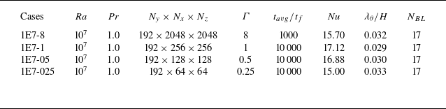
 Ra=107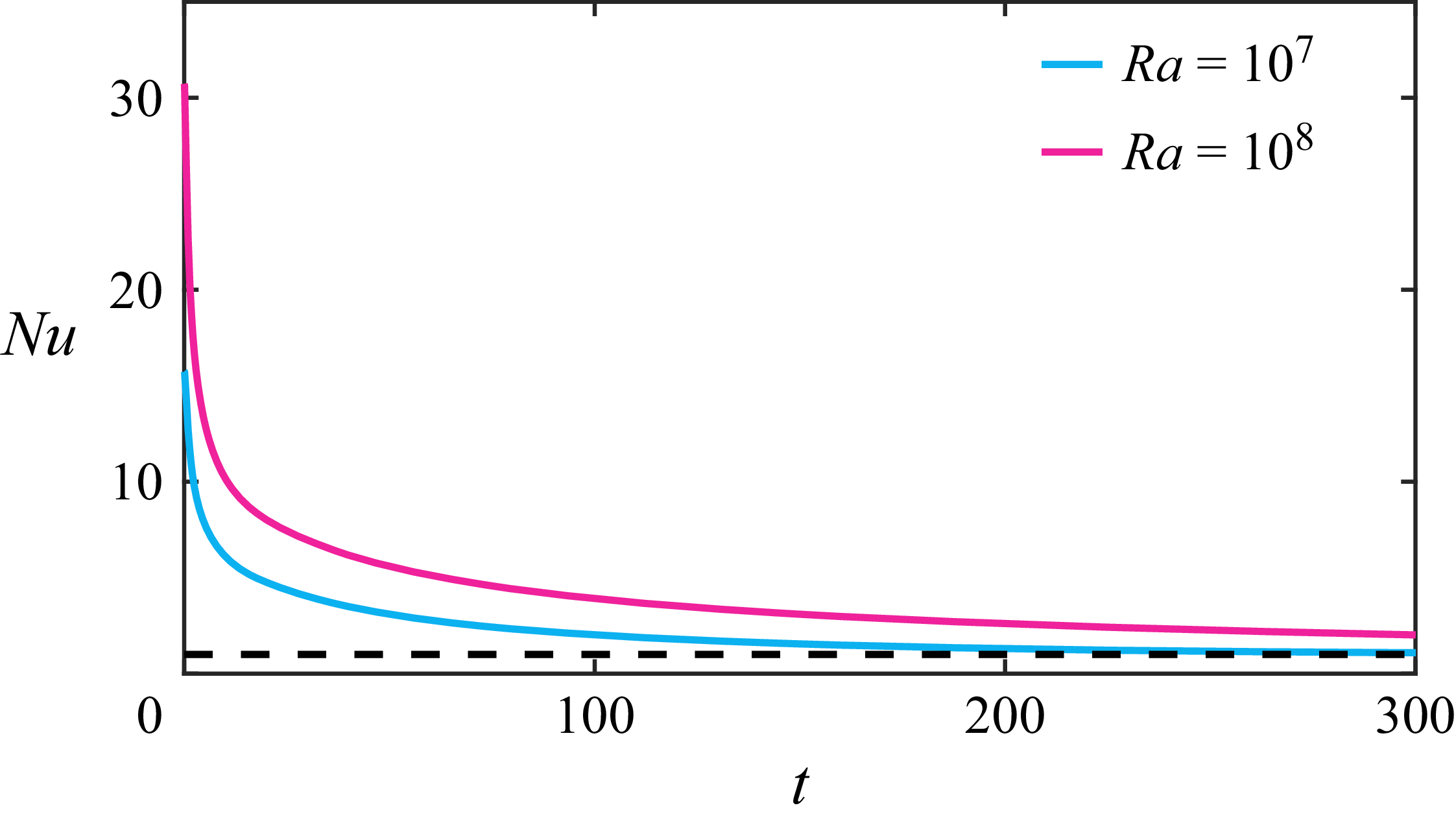
 Nu
Nu tf=H/(αgΔ)
 t=0
t=0 Nu=1
Nu=1
 dΘ/dy
dΘ/dy κθ~
κθ~ G
G t
t kx
kx Ra=107
 γ=0.01
 Ra=108
 γ=0.01
 Ra=107
 γ=100.0
 Ra=108
 γ=100.0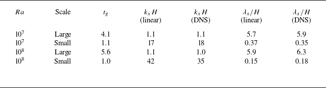
 tg
tg
 tg
tg tg
tg Ra=107
 γ=0.01
 tg=4.1tf
 Ra=108
 γ=0.01
 tg=5.6tf
 Ra=107
 γ=100.0
 tg=1.1tf
 Ra=108
 γ=100.0
 tg=1.0tf
 Ra=107
 dΘ/dy
dΘ/dy κθ~
κθ~ G
G t
t kx
kx γ=0.01
 γ=100.0
 Γ=8
Γ=8 Γ=1
Γ=1 Γ=0.5
Γ=0.5 Γ=0.25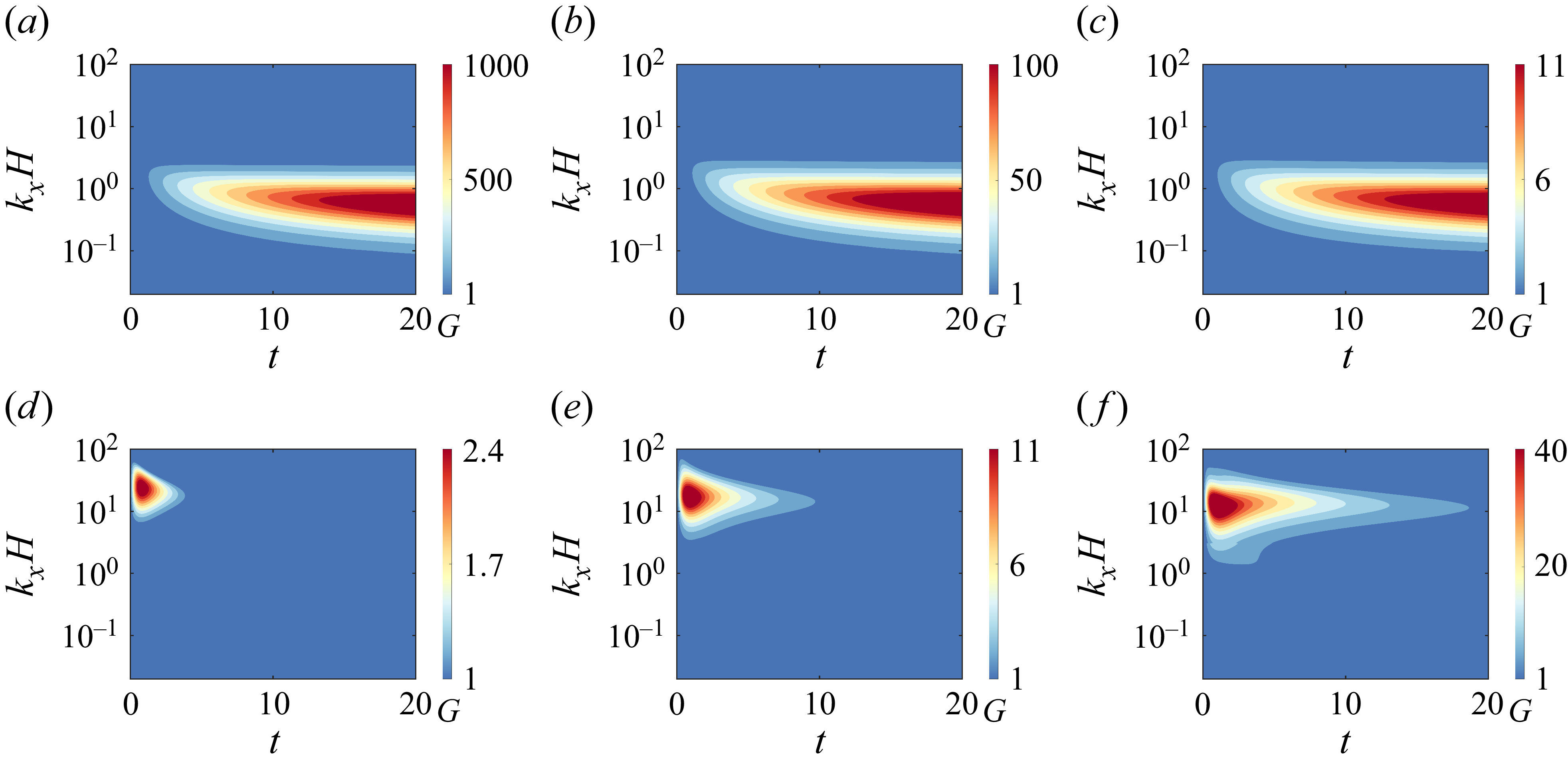
 G
G t
t kx
kx γ
γ 10−3
10−3 103
103 Ra=107
 γ=0.001
 0.01
0.01 0.1
0.1 10
10 100
100 1000
1000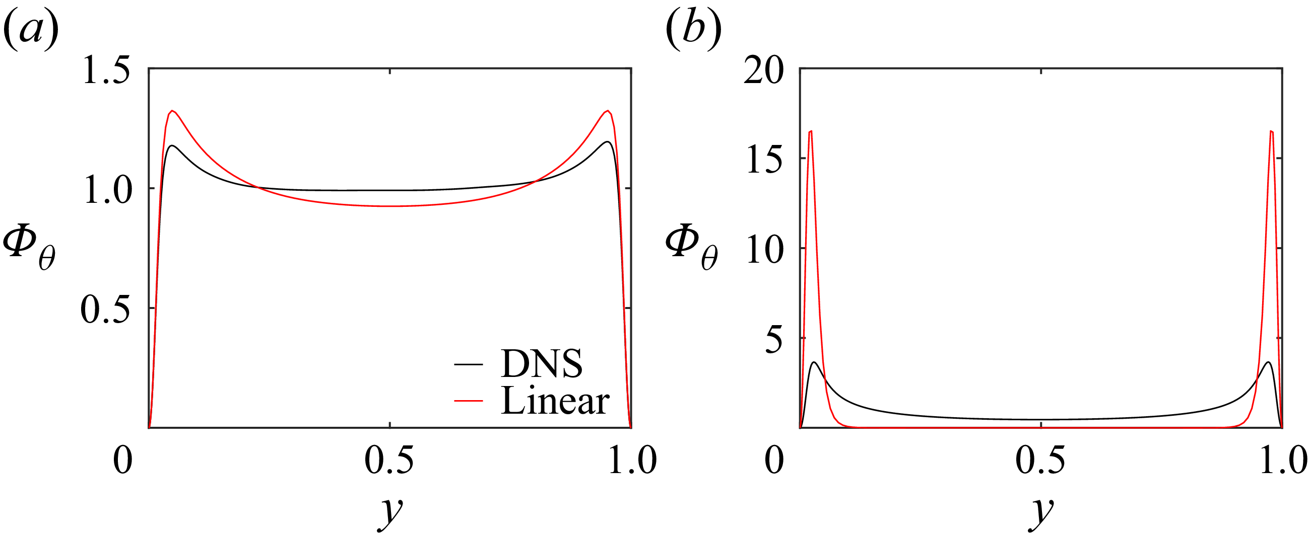
 Φθ
Φθ Φθ
Φθ
 Open access

