


1. Introduction
When a viscous fluid with a free surface is strongly driven, the free surface is often seen to deform into a cusp singularity, rounded at the tip on a small scale only. As long as the driving varies slowly in the third dimension, the tip position is close to a straight line, and the flow can be regarded as effectively two-dimensional. The formation of free-surface cusps was first highlighted and demonstrated experimentally by Joseph et al. (Reference Joseph, Nelson, Renardy and Renardy1991), placing two counter-rotating rollers beneath the free surface of a viscous fluid, dragging fluid into the space between them. The observed cusps were so sharp that it led Joseph et al. (Reference Joseph, Nelson, Renardy and Renardy1991) to propose that the free surface was indeed ending in a point, producing a non-differentiable surface even in the presence of surface tension.
To investigate this question, Jeong & Moffatt (Reference Jeong and Moffatt1992) constructed an exact solution to the two-dimensional viscous flow equations, driven by a vortex dipole underneath a free surface, using the method of complex mapping from the unit disk into the flow domain. They found that the tip size remains finite, but is exponentially small in the capillary number, which is the flow speed, made dimensionless using the capillary speed $\gamma /\eta$
. Here
$\gamma /\eta$
. Here $\gamma$
is the coefficient of surface tension between the liquid and an inert exterior gas and
$\gamma$
is the coefficient of surface tension between the liquid and an inert exterior gas and $\eta$
is the shear viscosity of the liquid. This exponential dependence was later verified experimentally by Lorenceau, Restagno & Quéré (Reference Lorenceau, Restagno and Quéré2003), using an apparatus similar to that used by Joseph et al. (Reference Joseph, Nelson, Renardy and Renardy1991) and Jeong & Moffatt (Reference Jeong and Moffatt1992).
$\eta$
is the shear viscosity of the liquid. This exponential dependence was later verified experimentally by Lorenceau, Restagno & Quéré (Reference Lorenceau, Restagno and Quéré2003), using an apparatus similar to that used by Joseph et al. (Reference Joseph, Nelson, Renardy and Renardy1991) and Jeong & Moffatt (Reference Jeong and Moffatt1992).
Cusps play an important role in free-surface flow, because they provide a key mechanism for the entrainment of air into a liquid bath (Kiger & Duncan Reference Kiger and Duncan2012). Owing to the exponential shrinkage of the tip size with capillary number, the gap inside the cusp becomes extremely narrow. This means that an external fluid (such as air), which is drawn into the cusp, leads to an elevated lubrication pressure inside the narrow gap, which eventually leads to a bifurcation (Eggers Reference Eggers2001; Lorenceau, Quéré & Eggers Reference Lorenceau, Quéré and Eggers2004), even if the viscosity of the outer liquid is much smaller than that of the bath. As a result of the bifurcation, a sheet of air is drawn into the liquid (Lorenceau et al. Reference Lorenceau, Quéré and Eggers2004), opening a channel for air entrainment. In the present paper, however, we will disregard the effect of any external fluid, and focus on the formation of the cusp and its relation to the driving flow.
Following Jeong & Moffatt (Reference Jeong and Moffatt1992), many more exact two-dimensional solutions similar to theirs were constructed using the method introduced by Richardson (Reference Richardson1968), placing various singularities underneath a flat surface (Jeong & Moffatt Reference Jeong and Moffatt1992; Jeong Reference Jeong1999, Reference Jeong2010, Reference Jeong2007), or near a two-dimensional ‘bubble’ (Antanovskii Reference Antanovskii1996; Cummings & Howison Reference Cummings and Howison1999; Cummings Reference Cummings2000; Crowdy Reference Crowdy2002). However, while instructive, no number of exact solutions for a specific geometry and driving explains the mathematical structure of the cusp, and the local balance underlying it. In particular, Jeong & Moffatt (Reference Jeong and Moffatt1992) found their interface profile to exhibit the form of a similarity solution near the tip. Its form corresponds exactly to the generic singularity of a planar curve near a point of self-intersection (Eggers & Fontelos Reference Eggers and Fontelos2012, Reference Eggers and Fontelos2015), as found in singularity (bifurcation) theory (Eggers & Suramlishvili Reference Eggers and Suramlishvili2017).
This suggests that singularities of higher order can also be realised in Stokes flow, and that there are deep connections with other free-surface flows (Eggers & Fontelos Reference Eggers and Fontelos2012), such as Hele-Shaw flow (Howison Reference Howison1986) or potential flow (Mallet-Paret Reference Mallet-Paret1980). This connection has been explored further in a series of papers (Howison & Richardson Reference Howison and Richardson1995; Cummings & Howison Reference Cummings and Howison1999; Cummings, Howison & King Reference Cummings, Howison and King1999), but always relying on a particular set of exact solutions, furnished by complex mappings. Instead, we aim to understand the structure of the solution in its full generality, relying on local arguments only.
The problem of finding local cusp solutions has recently been addressed by one of us (Eggers Reference Eggers2023), using a boundary integral method. However, the necessary calculations are quite involved, and the integral formulation obscures the simple force balance expressed by the equations of fluid motion. Instead, here we pursue an alternative approach proposed in Morgan (Reference Morgan1994), Howison, Morgan & Ockendon (Reference Howison, Morgan and Ockendon1997) and Gillow (Reference Gillow1998), which relies on the slenderness of the cusp, and which has been applied to a wide range of potential flow, Hele-Shaw flow and Stokes flow problems with and without surface tension. The stationary cusp in Stokes flow with surface tension, inspired by the exact solution of Jeong & Moffatt (Reference Jeong and Moffatt1992), has, however, not yet been considered in this way.
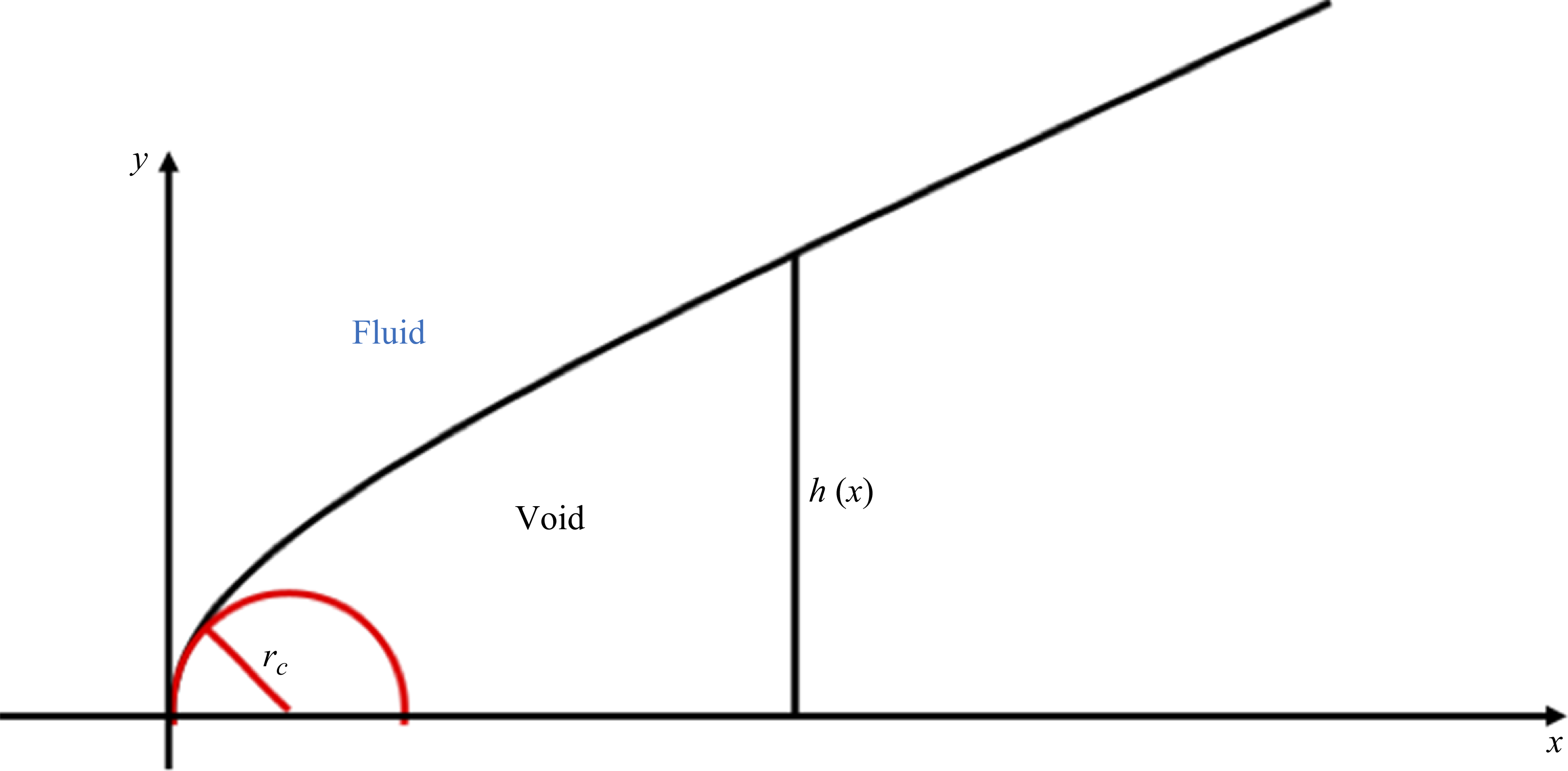
In the following, we assume that all lengths have been made dimensionless using some external length scale $L$
, which is a feature of the particular geometry of the apparatus at hand. In the example of the solution of Jeong & Moffatt (Reference Jeong and Moffatt1992), in which the flow is driven by a vortex dipole underneath a free surface, this could be the depth of the dipole in its rest state of vanishing dipole strength. Velocities are measured in units of the capillary speed
$L$
, which is a feature of the particular geometry of the apparatus at hand. In the example of the solution of Jeong & Moffatt (Reference Jeong and Moffatt1992), in which the flow is driven by a vortex dipole underneath a free surface, this could be the depth of the dipole in its rest state of vanishing dipole strength. Velocities are measured in units of the capillary speed $\gamma /\eta$
, so that
$\gamma /\eta$
, so that $\eta L / \gamma$
is a time scale. We are solving the two-dimensional, steady, viscous flow equations with a free surface, written as
$\eta L / \gamma$
is a time scale. We are solving the two-dimensional, steady, viscous flow equations with a free surface, written as $y = h(x)$
, and assuming symmetry about the
$y = h(x)$
, and assuming symmetry about the $x$
axis (see figure 1). The viscous flow equation in the bulk is
$x$
axis (see figure 1). The viscous flow equation in the bulk is
 \begin{equation} {\boldsymbol{\nabla }} p = \triangle \boldsymbol {v}, \end{equation}
where $\boldsymbol {v} = (u,v)$
is a two-dimensional velocity field and
$\boldsymbol {v} = (u,v)$
is a two-dimensional velocity field and $p$
the pressure. On the free surface (
$p$
the pressure. On the free surface ( $\boldsymbol{\sigma }$
is the stress tensor) the stress boundary condition reads
$\boldsymbol{\sigma }$
is the stress tensor) the stress boundary condition reads
 \begin{equation} \boldsymbol {n}\boldsymbol{\cdot }\boldsymbol{\sigma } = \frac {h''}{\left (1 + h'^2\right )^{3/2}}\boldsymbol {n}, \end{equation}
where a prime denotes the derivative with respect to the argument and $\boldsymbol {n}$
is the normal to the free surface. The condition for a steady flow is
$\boldsymbol {n}$
is the normal to the free surface. The condition for a steady flow is
 \begin{equation} h' = \frac {v}{u}. \end{equation}
Equations (1.1)–(1.3) have been made dimensionless using the length $L$
, time scale
$L$
, time scale $\eta L / \gamma$
and pressure scale
$\eta L / \gamma$
and pressure scale $\gamma /L$
. We aim to solve (1.1)–(1.3) in the limit that the radius of curvature of the tip
$\gamma /L$
. We aim to solve (1.1)–(1.3) in the limit that the radius of curvature of the tip $r_c$
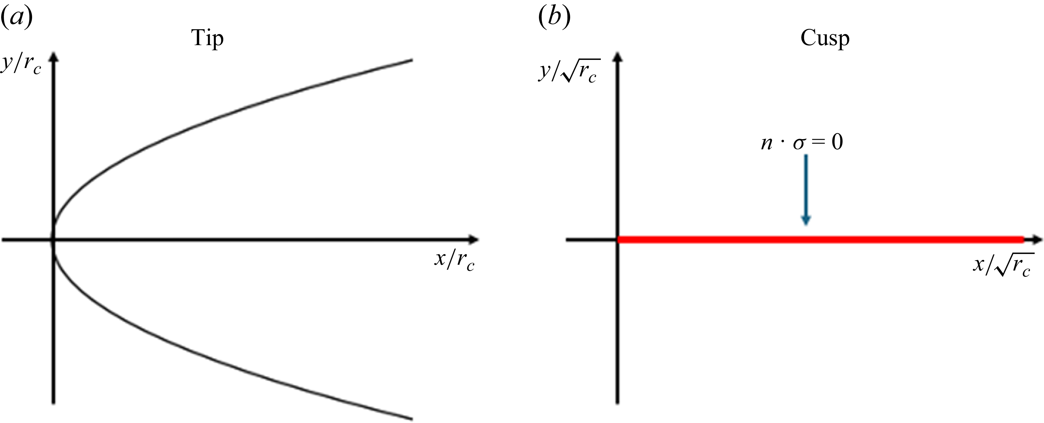
(see figure 1) tends to zero.
$r_c$
(see figure 1) tends to zero.
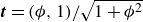
A sketch of the cusp geometry, symmetric about the $x$
axis: the shape is described by
$x$
axis: the shape is described by $h(x)$
, there is a viscous fluid outside and the inside of the cusp contains a gas which does not exert any stress. The tip of the cups is rounded, with
$h(x)$
, there is a viscous fluid outside and the inside of the cusp contains a gas which does not exert any stress. The tip of the cups is rounded, with $r_c$
the radius of curvature.
$r_c$
the radius of curvature.

2. Asymptotic solution
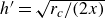
Our solution proceeds by matching two asymptotic regions shown schematically in figure 2. The tip region plays the role of an inner solution, the cusp region is the outer solution. We begin by describing both regions individually, and then show in more detail how they are matched.
(a) The inner (tip) region, which has typical scale $r_c$
; the interface reduces to a parabola in the limit
$r_c$
; the interface reduces to a parabola in the limit $r_c\rightarrow 0$
. (b) In the outer (cusp) region, the interface reduces to the positive
$r_c\rightarrow 0$
. (b) In the outer (cusp) region, the interface reduces to the positive $x$
axis when viewed on scale
$x$
axis when viewed on scale $\sqrt {r_c}$
, with
$\sqrt {r_c}$
, with $r_c\rightarrow 0$
.
$r_c\rightarrow 0$
.

2.1. The tip region
The tip region has the form of a parabola $h = \sqrt {2 r_c} x^{1/2}$
, where
$h = \sqrt {2 r_c} x^{1/2}$
, where $r_c$
is the radius of curvature. This shape, together with an appropriate velocity field, is an exact steady solution of the Stokes equation with surface tension (Hopper Reference Hopper1993). This can be shown by solving the equations using the mapping
$r_c$
is the radius of curvature. This shape, together with an appropriate velocity field, is an exact steady solution of the Stokes equation with surface tension (Hopper Reference Hopper1993). This can be shown by solving the equations using the mapping
 \begin{equation} z = 2 r_c w(\zeta ) \equiv 2r_c\left (\zeta ^2 + {\rm i}\zeta \right )\!, \end{equation}
where $\zeta$
real corresponds to the free surface. Thus the upper half of the
$\zeta$
real corresponds to the free surface. Thus the upper half of the $\zeta$
plane is mapped into the fluid domain, which is the outside of the cusp. In the Goursat representation (Jeong & Moffatt Reference Jeong and Moffatt1992), the streamfunction of the flow is written in terms of two holomorphic functions
$\zeta$
plane is mapped into the fluid domain, which is the outside of the cusp. In the Goursat representation (Jeong & Moffatt Reference Jeong and Moffatt1992), the streamfunction of the flow is written in terms of two holomorphic functions $f$
and
$f$
and $g$
:
$g$
:
 \begin{equation} \psi = {\rm Im} \left \{f(z) + \bar {z}g(z)\right \}; \end{equation}
the components of the velocity field are calculated from $u = \psi _y$
and
$u = \psi _y$
and $v = -\psi _x$
, where the subscript denotes the derivative. However, in the complex formulation the velocity field is recovered more conveniently from
$v = -\psi _x$
, where the subscript denotes the derivative. However, in the complex formulation the velocity field is recovered more conveniently from
 \begin{equation} u - {\rm i}v = f'(z) + \bar {z}g'(z) - \overline {g(z)}. \end{equation}
As shown in Hopper (Reference Hopper1993), the steady flow around the parabola (2.1) is given by
 \begin{equation} f = \frac {{\rm i} r_c}{2} w'(\zeta )\bar {w}(\zeta ) G(\zeta ), \quad g = -\frac {{\rm i}}{2} w'(\zeta ) G(\zeta ), \end{equation}
where
 \begin{align} G = \frac {1}{2\pi {\rm i} \sqrt {1 + 4\zeta ^2}} \ln \left (\frac {2\zeta -\sqrt {1 + 4\zeta ^2}} {2\zeta +\sqrt {1 + 4\zeta ^2}}\right ) \end{align}
and $\bar {w}(\zeta )=\overline {w(\bar {\zeta })}$
is the conjugate function.
$\bar {w}(\zeta )=\overline {w(\bar {\zeta })}$
is the conjugate function.
The free surface can be parametrised by putting $\zeta = \phi /2$
, with
$\zeta = \phi /2$
, with $\phi$
real, the tangent vector to the parabola is
$\phi$
real, the tangent vector to the parabola is $\boldsymbol {t} = (\phi ,1)/\sqrt {1 + \phi ^2}$
and thus the tangential velocity
$\boldsymbol {t} = (\phi ,1)/\sqrt {1 + \phi ^2}$
and thus the tangential velocity $u_0$
is found from
$u_0$
is found from $ u_0 = (u\phi + v)/\sqrt {1 + \phi ^2}$
. Using the solution (2.4), this gives
$ u_0 = (u\phi + v)/\sqrt {1 + \phi ^2}$
. Using the solution (2.4), this gives
 \begin{equation} u_0(\phi ) = -\frac {1}{\pi }\ln \left (\sqrt {1 + \phi ^2}+\phi \right )\!, \quad \phi = \sqrt {2 x/r_c}, \end{equation}
in agreement with Eggers (Reference Eggers2023); the velocity near the interface can be inferred from
 \begin{align} (u,v) = \frac {(1,h^\prime )}{\sqrt {1+h^{\prime 2}}} u_0 . \end{align}
In the far field, along the interface
 \begin{equation} u_0 = -\frac {1}{2\pi }\ln \frac {8x}{r_c}, \end{equation}
which is the far field of a stokeslet, i.e. the velocity field generated by a point force of strength $2$
. This corresponds to each side of the interface pulling with force
$2$
. This corresponds to each side of the interface pulling with force $\gamma$
(per unit length in the third direction). Since
$\gamma$
(per unit length in the third direction). Since $h' = \sqrt {r_c/(2x)}$
, which vanishes for
$h' = \sqrt {r_c/(2x)}$
, which vanishes for $x\rightarrow \infty$
, we have
$x\rightarrow \infty$
, we have
 \begin{equation} u = -\frac {1}{2\pi }\ln \frac {8x}{r_c}, \quad v = -\frac {\sqrt {r_c}}{2^{3/2}\pi \sqrt {x}}\ln \frac {8x}{r_c}, \end{equation}
again for large $x$
.
$x$
.
2.2. The cusp region
In the cusp region, we can make use of slenderness and model the air gap as a cut in the complex plane along the positive $x$
axis, as illustrated in figure 2(b); this is confirmed more formally below. We are seeking solutions to the Stokes equation symmetric about the
$x$
axis, as illustrated in figure 2(b); this is confirmed more formally below. We are seeking solutions to the Stokes equation symmetric about the $x$
axis and with stress-free conditions along the positive
$x$
axis and with stress-free conditions along the positive $x$
axis, valid locally around the tip of the cusp, which is at the origin. This is justified by the crucial observation that the stokeslet solution does not contribute to the stress at leading order, as we see below.
$x$
axis, valid locally around the tip of the cusp, which is at the origin. This is justified by the crucial observation that the stokeslet solution does not contribute to the stress at leading order, as we see below.
Since the asymptotic problem of a cut of vanishing thickness is lacking a characteristic length scale, we seek power-law solutions for the streamfunction of the form (Eggers & Fontelos Reference Eggers and Fontelos2015)
 \begin{equation} \psi = r^{\lambda }\left [A\sin (\lambda \varphi ) + C\sin ((\lambda -2)\varphi )\right ], \end{equation}
where $r$
is the distance from the tip and
$r$
is the distance from the tip and $\varphi$
the angle measured from the negative
$\varphi$
the angle measured from the negative $x$
axis. This ensures that the line
$x$
axis. This ensures that the line $\varphi =0$
in the wake of the cusp is a streamline, while the surface of the cusp is at
$\varphi =0$
in the wake of the cusp is a streamline, while the surface of the cusp is at $\varphi =\pi$
. Expansions of this form are standard in two-dimensional solid mechanics (see e.g. Muskhelishvili Reference Muskhelishvili1953; Gakhov Reference Gakhov1966). As shown in detail in Eggers & Fontelos (Reference Eggers and Fontelos2015), eliminating the pressure and demanding that the two components of the stress vanish at the free surface
$\varphi =\pi$
. Expansions of this form are standard in two-dimensional solid mechanics (see e.g. Muskhelishvili Reference Muskhelishvili1953; Gakhov Reference Gakhov1966). As shown in detail in Eggers & Fontelos (Reference Eggers and Fontelos2015), eliminating the pressure and demanding that the two components of the stress vanish at the free surface $\varphi =\pi$
lead to the conditions
$\varphi =\pi$
lead to the conditions $\sin \lambda \pi = 0$
or
$\sin \lambda \pi = 0$
or $\cos \lambda \pi = 0$
for the scaling exponent
$\cos \lambda \pi = 0$
for the scaling exponent $\lambda$
.
$\lambda$
.
The first class of solutions leads to integer $\lambda$
, with vanishing transversal velocity
$\lambda$
, with vanishing transversal velocity $v=0$
along the cusp surface
$v=0$
along the cusp surface $x\gt 0$
. Non-singular velocity fields correspond to
$x\gt 0$
. Non-singular velocity fields correspond to $\lambda = 1,2,\ldots$
, yielding
$\lambda = 1,2,\ldots$
, yielding $u = x^n,\;n=0,1,\ldots$
for the tangential velocity along the cusp surface. Thus with
$u = x^n,\;n=0,1,\ldots$
for the tangential velocity along the cusp surface. Thus with $-U$
being the leading-order velocity sweeping past the cusp, a general superposition of these solutions yields the tangential velocity
$-U$
being the leading-order velocity sweeping past the cusp, a general superposition of these solutions yields the tangential velocity
 \begin{equation} u = -U + b_1 x + b_2 x^2 + \cdots , \end{equation}
with $b_i$
being parameters. On the other hand, the second condition (and avoiding solutions too singular to match to the parabolic solution (2.4)), leads to
$b_i$
being parameters. On the other hand, the second condition (and avoiding solutions too singular to match to the parabolic solution (2.4)), leads to $\lambda = 1/2,3/2,\ldots$
. Then on the positive
$\lambda = 1/2,3/2,\ldots$
. Then on the positive $x$
axis, the velocity corresponding to these values is normal to the cusp, so that up to normalisation
$x$
axis, the velocity corresponding to these values is normal to the cusp, so that up to normalisation $u=0$
,
$u=0$
, $v = \pm x^{(2n-1)/2},\; n=0,1,2,\ldots$
, above and below the gap, respectively. This means a general superposition of normal velocities is of the form
$v = \pm x^{(2n-1)/2},\; n=0,1,2,\ldots$
, above and below the gap, respectively. This means a general superposition of normal velocities is of the form
 \begin{equation} u = 0, \quad v = a_0 x^{-1/2} + a_1 x^{1/2} + \cdots , \end{equation}
once more with $a_i$
as free parameters.
$a_i$
as free parameters.
In addition to (2.10), another solution to the Stokes equation in the presence of a gap is a stokeslet of strength unity, pulling in the positive $x$
direction (Pozrikidis Reference Pozrikidis1992):
$x$
direction (Pozrikidis Reference Pozrikidis1992):
 \begin{equation} \psi = -\frac {y}{4\pi }\ln (r/a); \end{equation} $a$
is a positive constant. Solution (2.13) is distinct from (2.11) and (2.12), in that it breaks scale invariance.
$a$
is a positive constant. Solution (2.13) is distinct from (2.11) and (2.12), in that it breaks scale invariance.
Once more both components of the normal stress generated by (2.13) vanish on the surface $y=0$
. Now the velocity on the positive
$y=0$
. Now the velocity on the positive $x$
axis corresponding to (2.13) is
$x$
axis corresponding to (2.13) is $u = -\ln (x/a)/(4\pi )$
and
$u = -\ln (x/a)/(4\pi )$
and $v = 0$
, which matches (2.9) for a stokeslet of strength
$v = 0$
, which matches (2.9) for a stokeslet of strength $2$
, and putting
$2$
, and putting $a = r_c/8$
. This means that the total tangential component of the velocity is of the form
$a = r_c/8$
. This means that the total tangential component of the velocity is of the form
 \begin{equation} u = -\frac {1}{2\pi }\ln \left (\frac {8x}{r_c}\right ) + b_1 x + b_2 x^2 + \cdots . \end{equation}
The leading-order contribution to (2.12) for which $v$
remains finite at
$v$
remains finite at $x=0$
is
$x=0$
is $a_1x^{1/2}$
; this is the one considered in Joseph et al. (Reference Joseph, Nelson, Renardy and Renardy1991) and Eggers & Fontelos (Reference Eggers and Fontelos2015). Together with a constant down-streaming
$a_1x^{1/2}$
; this is the one considered in Joseph et al. (Reference Joseph, Nelson, Renardy and Renardy1991) and Eggers & Fontelos (Reference Eggers and Fontelos2015). Together with a constant down-streaming $u=-U$
(which is the leading contribution to (2.11)), this produces a cusp which opens with a
$u=-U$
(which is the leading contribution to (2.11)), this produces a cusp which opens with a $3/2$
exponent. The crucial observation is that in order to match to the parabolic solution, we also have to add
$3/2$
exponent. The crucial observation is that in order to match to the parabolic solution, we also have to add $a_0 x^{-1/2}$
to obtain
$a_0 x^{-1/2}$
to obtain
 \begin{equation} u = -U + b_1 x, \quad v = a_0 x^{-1/2} + a_1 x^{1/2}, \end{equation}
with higher-order terms discarded.
Then since the interface is a streamline in steady state, we obtain for the slope
 \begin{equation} h' = \frac {v}{u} = -\frac {a_0}{U}x^{-1/2} - \left (\frac {a_1}{U} - \frac {a_0 b_1}{U^2}\right ) x^{1/2} + O\bigl(x^{3/2}\bigr). \end{equation}
Thus identifying
 \begin{equation} r_c = 2\left (\frac {a_0}{U}\right )^2, \quad c = -\frac {2a_1}{3U} + \frac {a_0b_1}{U^2}, \end{equation}
and integrating (2.16), this yields
 \begin{equation} h = \sqrt {2 r_c} x^{1/2} + c x^{3/2}, \end{equation}
which is precisely the self-similar cusp profile found originally by Jeong & Moffatt (Reference Jeong and Moffatt1992). Again, higher-order terms have been discarded in order to obtain the leading-order shape valid near the cusp tip. This is the central result of this paper, in which the structure of the cusp is obtained by local analysis of the flow equations alone.
For small $x$
, (2.18) agrees with the parabolic solution (2.1). On the other hand, to leading order as
$x$
, (2.18) agrees with the parabolic solution (2.1). On the other hand, to leading order as $r_c\rightarrow 0$
, comparing (2.14) and (2.11) provides the down-streaming velocity
$r_c\rightarrow 0$
, comparing (2.14) and (2.11) provides the down-streaming velocity $U\gt 0$
:
$U\gt 0$
:
 \begin{equation} U = -\frac {1}{2\pi }\ln \frac {r_c}{8}, \end{equation}
which reveals an exponential dependence of the tip curvature on the externally imposed flow, as found originally by Jeong & Moffatt (Reference Jeong and Moffatt1992).
2.3. Matching
We now make sure that the solution proposed above is consistent in the limit $r_c\rightarrow 0$
, and that the different parts match. From (2.18) we see that the two terms on the right are balanced for
$r_c\rightarrow 0$
, and that the different parts match. From (2.18) we see that the two terms on the right are balanced for $x = O(r_c^{1/2})$
, so that both terms are of
$x = O(r_c^{1/2})$
, so that both terms are of $O(r_c^{3/4})$
. For
$O(r_c^{3/4})$
. For $x$
of the order of
$x$
of the order of $r_c$
, we are in the tip region; conversely for
$r_c$
, we are in the tip region; conversely for $x$
on the scale of
$x$
on the scale of $\sqrt {r_c}$
, we are in the cusp region, as shown in figure 2. It follows that (2.18) can be written in self-similar form as
$\sqrt {r_c}$
, we are in the cusp region, as shown in figure 2. It follows that (2.18) can be written in self-similar form as
 \begin{equation} y = r_c^{3/4} H\bigl(x/r_c^{1/2}\bigr), \quad H(\xi ) = (2\xi )^{1/2} + c\xi ^{3/2}, \end{equation}
where $c$
remains a free parameter, which depends on the particular problem at hand. The similarity solution (2.20) is precisely of the form found by Jeong & Moffatt (Reference Jeong and Moffatt1992) for a vortex dipole underneath an infinitely extended free surface, and thus for a specific value of the constant
$c$
remains a free parameter, which depends on the particular problem at hand. The similarity solution (2.20) is precisely of the form found by Jeong & Moffatt (Reference Jeong and Moffatt1992) for a vortex dipole underneath an infinitely extended free surface, and thus for a specific value of the constant $c$
only. Our calculation now demonstrates that (2.20) is the generic structure of the cusp, and establishes
$c$
only. Our calculation now demonstrates that (2.20) is the generic structure of the cusp, and establishes $c$
as the only free parameter, once the radius of curvature
$c$
as the only free parameter, once the radius of curvature $r_c$
is taken as a reference length scale.
$r_c$
is taken as a reference length scale.
The structure of the matching problem is illustrated in figure 2. In figure 2(a), we show the inner, tip problem, which lives on scale $r_c$
. It represents an exact solution to the Stokes equation with a free surface, which happens to be a parabola. Putting
$r_c$
. It represents an exact solution to the Stokes equation with a free surface, which happens to be a parabola. Putting $\bar {x} = x/r_c$
and
$\bar {x} = x/r_c$
and $\bar {y} = y/r_c$
, this free surface can be written as
$\bar {y} = y/r_c$
, this free surface can be written as
 \begin{equation} \bar {y} = \sqrt {2\bar {x}}. \end{equation}
In figure 2(b), we illustrate the outer, cusp solution on scale $\sqrt {r_c}$
. It follows from (2.20) that in the limit
$\sqrt {r_c}$
. It follows from (2.20) that in the limit $r_c\rightarrow 0$
the surface degenerates to a line, occupying the positive
$r_c\rightarrow 0$
the surface degenerates to a line, occupying the positive $x$
axis, shown as the thick red line. Moreover, we show that to leading order the boundary condition on the cut is stress-free, as assumed in deriving solutions (2.11)–(2.13). First, using the scaling (2.20), we estimate the curvature in (1.2) as
$x$
axis, shown as the thick red line. Moreover, we show that to leading order the boundary condition on the cut is stress-free, as assumed in deriving solutions (2.11)–(2.13). First, using the scaling (2.20), we estimate the curvature in (1.2) as $\kappa = O(r_c^{3/4}/\sqrt {r_c}^2) = O(r_c^{-1/4})$
. Second, to estimate the stress, we note that the stokeslet solution (2.13), for which
$\kappa = O(r_c^{3/4}/\sqrt {r_c}^2) = O(r_c^{-1/4})$
. Second, to estimate the stress, we note that the stokeslet solution (2.13), for which $v=0$
, does not contribute to the stress. At next order, combining (2.15) and (2.17), we have
$v=0$
, does not contribute to the stress. At next order, combining (2.15) and (2.17), we have $v \approx a_0 x^{-1/2} = O(\sqrt {r_c/x}\ln r_c)$
. Estimating the derivative at scale
$v \approx a_0 x^{-1/2} = O(\sqrt {r_c/x}\ln r_c)$
. Estimating the derivative at scale $\sqrt {r_c}$
, we find
$\sqrt {r_c}$
, we find
 \begin{equation} \sigma = O\left(\sqrt {r_c/x^3}\ln r_c\right) = O\left(r_c^{-1/4}\ln r_c\right)\!, \end{equation}
which dominates the curvature by a logarithmic factor, and justifies looking for stress-free cusp solutions. This is a key observation, which explains why in spite of the complexity of the velocity field, which contains logarithmic contributions (e.g. (2.3)), finding cusp solutions reduces to finding solutions to the Stokes equation in the ’cut plane’ domain of figure 2.
Finally, we confirm the matching between the inner and outer velocity fields by comparing the outer limit of the inner solution with the inner limit of the outer solution. In the limit $r_c\rightarrow 0$
,we find from (2.9) (the inner solution):
$r_c\rightarrow 0$
,we find from (2.9) (the inner solution):
 \begin{equation} u = \frac {1}{2\pi }\ln \frac {r_c}{8} = -U, \quad v = \frac {\sqrt {r_c}}{2^{3/2}\pi \sqrt {x}}\ln \frac {r_c}{8} = \sqrt {\frac {r_c}{2x}} U, \end{equation}
using (2.19). If one considers the inner limit of (2.12), one obtains $v = a_1 x^{-1/2} = \sqrt {r_c/2} U x^{-1/2}$
, which is the second equation of (2.23), which demonstrates the required matching.
$v = a_1 x^{-1/2} = \sqrt {r_c/2} U x^{-1/2}$
, which is the second equation of (2.23), which demonstrates the required matching.
2.4. The outer flow
The flow defined by (2.14) has the property that it is not bounded at infinity, so one might worry that it cannot be matched to a finite outer flow. We now show that this is not a limitation of the present approach. Rather, solutions of the form (2.11) can be superimposed to produce bounded velocities. To see that, it is advantages to use the complex representation (2.2), in which solutions $u=x^n$
are described by
$u=x^n$
are described by
 \begin{equation} f(z) = \frac {z^{n+1}}{2}, \quad g(z) = \frac {z^n}{2}. \end{equation}
Indeed, the streamfunction is
 \begin{equation} \psi = \frac {1}{2}{\rm Im} \{z^{n+1}-\bar {z}z^n\} = y\,{\rm Im} \{i z^n\} = y x^n, \end{equation}
so we recover $u = \partial _y\psi = x^n$
. Similarly, the streamfunction of a stokeslet (2.13) can be written
$u = \partial _y\psi = x^n$
. Similarly, the streamfunction of a stokeslet (2.13) can be written $\psi = y\,{\rm Re} \{\ln z\}$
.
$\psi = y\,{\rm Re} \{\ln z\}$
.
Superimposing the solutions (2.25), we can write in general
 \begin{equation} \psi = y\, {\rm Re} \{\chi (z)\}, \quad \mbox{with}\; \chi (z) = d_0\ln z + \sum _{n=0}^{\infty } d_{n+1} z^n. \end{equation}
By choosing
 \begin{equation} \chi (z) = -\frac {1}{2\pi }\ln \frac {8 z}{r_c} + \frac {1}{4\pi } \sum _{n=1}^{\infty }(-1)^{n+1}\frac {{\rm e}^{-4\pi nU}(8z)^{2n}}{r_c^{2n}} = \frac {1}{4\pi }\ln \left ({\rm e}^{-4\pi U} + \frac {r_c^2}{(8z)^2}\right )\!, \end{equation}
we have constructed a solution which for $z\rightarrow 0$
behaves like (2.14). On the other hand, for
$z\rightarrow 0$
behaves like (2.14). On the other hand, for $z\rightarrow \infty$
we have
$z\rightarrow \infty$
we have $\chi \approx -U$
, implying that a finite tangential velocity
$\chi \approx -U$
, implying that a finite tangential velocity $u \approx -U$
is reached at infinity.
$u \approx -U$
is reached at infinity.
Looking at the behaviour of $\chi$
in the complex plane, and using (2.19), one obtains
$\chi$
in the complex plane, and using (2.19), one obtains
 \begin{equation} \chi = \frac {1}{4\pi }\ln \left (r_c^2 + \frac {r_c^2}{(8z)^2}\right ) = \frac {1}{2\pi }\ln \frac {r_c}{8z} + \frac {1}{4\pi }\ln \left (z - {\rm i}\right ) + \frac {1}{4\pi }\ln \left (z + {\rm i}\right )\!, \end{equation}
which has logarithmic singularities at $z = \pm {\rm i}$
, or
$z = \pm {\rm i}$
, or $y = \pm 1$
. According to (2.26), this means that near the singularities
$y = \pm 1$
. According to (2.26), this means that near the singularities
 \begin{align} \psi = \pm \frac {1}{4\pi }\ln \left (z\mp {\rm i}\right )\!, \end{align}
which are counter-rotating vortices of circulation $\varGamma = \mp 1/2$
situated at
$\varGamma = \mp 1/2$
situated at $z = \pm {\rm i}$
. This is very similar to the solution considered in Jeong (Reference Jeong2010), where the flow leading to a cusp is driven by a pair of vortices. This, in turn, can be seen as an idealisation of the experimental set-ups in Joseph et al. (Reference Joseph, Nelson, Renardy and Renardy1991) and Jeong & Moffatt (Reference Jeong and Moffatt1992), where the flow is driven by two counter-propagating rollers.
$z = \pm {\rm i}$
. This is very similar to the solution considered in Jeong (Reference Jeong2010), where the flow leading to a cusp is driven by a pair of vortices. This, in turn, can be seen as an idealisation of the experimental set-ups in Joseph et al. (Reference Joseph, Nelson, Renardy and Renardy1991) and Jeong & Moffatt (Reference Jeong and Moffatt1992), where the flow is driven by two counter-propagating rollers.
The particular solution considered in (2.27) is just one of the many different ways of driving a free surface to cusp formation. However, a common feature of any such solution is the presence of singularities, of which the two vortices of (2.28) are a particular example. More generally, $\chi$
has to satisfy the requirement that
$\chi$
has to satisfy the requirement that $\chi \sim \ln z$
as
$\chi \sim \ln z$
as $z\rightarrow 0$
, to represent the stokeslet generated at the tip. This implies that
$z\rightarrow 0$
, to represent the stokeslet generated at the tip. This implies that $z\chi '(z) \sim 1$
as
$z\chi '(z) \sim 1$
as $z\rightarrow 0$
: the combination
$z\rightarrow 0$
: the combination $z\chi '(z)$
is free of singularities at the origin. In addition, the assumed boundedness of the velocity field at infinity implies that
$z\chi '(z)$
is free of singularities at the origin. In addition, the assumed boundedness of the velocity field at infinity implies that $z\chi '(z)$
can only grow sublinearly at infinity.
$z\chi '(z)$
can only grow sublinearly at infinity.
But supposing that $z\chi '(z)$
is analytic in the entire complex plane implies a contradiction: by Liouville’s theorem, such an analytic function has to grow at least linearly at infinity, which would be inconsistent with the velocity remaining bounded. Thus, the existence of singularities inside the flow, such as in (2.28), is a feature of the matching conditions we imposed. There is of course an infinite variety of ways such singularities can be imposed, corresponding to various ways in which the flow is driven.
$z\chi '(z)$
is analytic in the entire complex plane implies a contradiction: by Liouville’s theorem, such an analytic function has to grow at least linearly at infinity, which would be inconsistent with the velocity remaining bounded. Thus, the existence of singularities inside the flow, such as in (2.28), is a feature of the matching conditions we imposed. There is of course an infinite variety of ways such singularities can be imposed, corresponding to various ways in which the flow is driven.
3. Discussion
3.1. Higher-order singularities
The remarkable property of the profile (2.18) is that it corresponds exactly to the generic singularity of a smooth, planar curve, which is being deformed smoothly to produce a self-intersection (Eggers & Fontelos Reference Eggers and Fontelos2015; Eggers & Suramlishvili Reference Eggers and Suramlishvili2017). At the critical point where intersection first occurs, the curve then produces a cusp $h \propto x^{3/2}$
, but the tip remains rounded on a small scale in the neighbourhood of that point. The generic behaviour near such critical points is described by the singularity theory (Arnol’d et al. Reference Arnol’d, Vasil’ev, Goryunov and Lyashko1993), with the planar case described in more detail in Eggers & Suramlishvili (Reference Eggers and Suramlishvili2017).
$h \propto x^{3/2}$
, but the tip remains rounded on a small scale in the neighbourhood of that point. The generic behaviour near such critical points is described by the singularity theory (Arnol’d et al. Reference Arnol’d, Vasil’ev, Goryunov and Lyashko1993), with the planar case described in more detail in Eggers & Suramlishvili (Reference Eggers and Suramlishvili2017).
We emphasise that the cusp solutions discussed here differ fundamentally from Hopper’s solution describing the coalescence of cylinders in viscous flow (Hopper Reference Hopper1990; Eggers, Sprittles & Snoeijer Reference Eggers, Sprittles and Snoeijer2025). First, the coalescence solution is time dependent, not stationary, as are our solutions. Second, Hopper’s solution is non-generic, in that it applies only to a very specific initial condition, in which two cylinders touch in a perfectly aligned fashion. Third, and most importantly, the similarity solution describing the gap between two coalescing cylinders corresponds to an ‘elliptic umbilic catastrophe’ (Eggers et al. Reference Eggers, Sprittles and Snoeijer2025), in the language of catastrophe theory (Poston & Stewart Reference Poston and Stewart1978), which differs qualitatively from the cusp solutions associated with self-intersection, considered here.
In the present cusp problem, the symmetry of our problem under reflection suggests putting $x = s^2$
, with
$x = s^2$
, with $s$
parameterising the curve. Then, (2.18) turns into the parameterised curve
$s$
parameterising the curve. Then, (2.18) turns into the parameterised curve
 \begin{equation} (s^2,\sqrt {2 r_c} s + c s^3). \end{equation}
Up to a rescaling of the axes, this corresponds to the unfolding of the germ $(s^2,s^3)$
(Eggers & Suramlishvili Reference Eggers and Suramlishvili2017), the latter being the singular curve at the critical point. The singularity theory demonstrates that up to smooth transformations, any deformation of the original germ can be written in the form
$(s^2,s^3)$
(Eggers & Suramlishvili Reference Eggers and Suramlishvili2017), the latter being the singular curve at the critical point. The singularity theory demonstrates that up to smooth transformations, any deformation of the original germ can be written in the form $(s^2,\mu _1 s + s^3)$
, where
$(s^2,\mu _1 s + s^3)$
, where $\mu _1$
is a parameter. But this is exactly of the form (3.1), again up to trivial rescaling.
$\mu _1$
is a parameter. But this is exactly of the form (3.1), again up to trivial rescaling.
It is surprising that the terms appearing in (3.1) only involve integer powers, as required by the singularity theory. This is a direct result of the fact that the stokeslet (2.13), although nominally the leading-order contribution to the velocity field, ends up making a subdominant contribution to the stress, as demonstrated by the estimate (2.22). As a result, logarithms do not appear in (2.15).
Thus, it is natural to generalise (3.1) to unfoldings of higher order, corresponding to higher-order terms in the sequence of powers appearing in (2.12) and (2.11). For example, if from the solution $v = a_n x^{(2n-1)/2}$
one chooses n = 2, and from (2.11) one takes the leading order contribution
$v = a_n x^{(2n-1)/2}$
one chooses n = 2, and from (2.11) one takes the leading order contribution $u = -U$
, one obtains
$u = -U$
, one obtains $h' = v/u = -(a_2/U) x^{3/2}$
. After integration, we obtain
$h' = v/u = -(a_2/U) x^{3/2}$
. After integration, we obtain $h = -2 a_2/(5 U) x^{5/2}$
, and hence we have generated the so-called
$h = -2 a_2/(5 U) x^{5/2}$
, and hence we have generated the so-called $A_4$
germ
$A_4$
germ $(s^2,s^5)$
(up to rescaling), discussed in detail in Eggers & Suramlishvili (Reference Eggers and Suramlishvili2017). As this germ is of higher order, one obtains a more general class of unfoldings, which are
$(s^2,s^5)$
(up to rescaling), discussed in detail in Eggers & Suramlishvili (Reference Eggers and Suramlishvili2017). As this germ is of higher order, one obtains a more general class of unfoldings, which are
 \begin{equation} (s^2,\mu _1 s + \mu _3 s^3 + s^5), \end{equation}
with two parameters $\mu _1$
and
$\mu _1$
and $\mu _3$
. But this is precisely the solution of Stokes’ equation one obtains when including terms with for
$\mu _3$
. But this is precisely the solution of Stokes’ equation one obtains when including terms with for $n=0, 1$
, and
$n=0, 1$
, and $2$
in the superposition (2.12).
$2$
in the superposition (2.12).
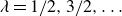
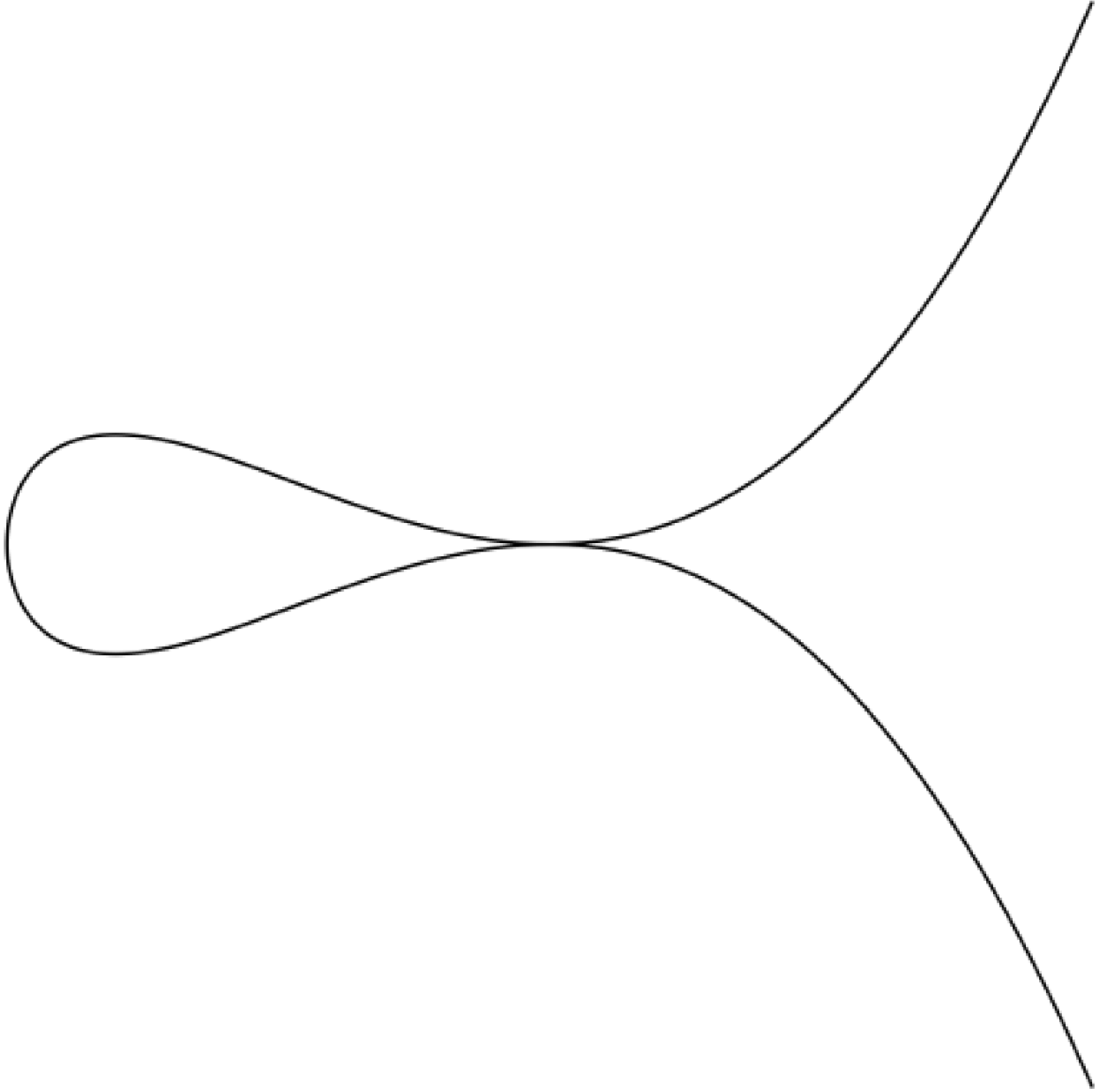
Left: A static solution to the Stokes equation, showing a bubble being enclosed at the tip of a cusp, as described by (3.3). The cusp opens like $h = x^{5/2}$
. Right: A shrinking two-dimensional bubble, with a source of unit strength at the centre, as described by (3.4) and (3.6) for
$h = x^{5/2}$
. Right: A shrinking two-dimensional bubble, with a source of unit strength at the centre, as described by (3.4) and (3.6) for $\hat {t} = 2,1,$
and
$\hat {t} = 2,1,$
and $0.5$
; the bubble vanishes for
$0.5$
; the bubble vanishes for $\hat {t} = 0$
.
$\hat {t} = 0$
.

In the generic case, in which $\mu _3 \ne 0$
has a finite value, the
$\mu _3 \ne 0$
has a finite value, the $s^3$
term will dominate over
$s^3$
term will dominate over $s^5$
near the tip of the cusp, and we fall back onto the standard profile (2.18). However, one can aim to adjust experimental conditions to reach a state of higher symmetry, at which the cubic term vanishes. Then, if we fine-tune the external flow such that
$s^5$
near the tip of the cusp, and we fall back onto the standard profile (2.18). However, one can aim to adjust experimental conditions to reach a state of higher symmetry, at which the cubic term vanishes. Then, if we fine-tune the external flow such that $\mu _3$
becomes small according to
$\mu _3$
becomes small according to $\mu _3 = -2\sqrt {\mu _1}$
as
$\mu _3 = -2\sqrt {\mu _1}$
as $\mu _1\rightarrow 0$
, a bubble is formed, whose shape is described by
$\mu _1\rightarrow 0$
, a bubble is formed, whose shape is described by
 \begin{equation} (x,y) = (s^2,s(s^2 - \sqrt {\mu _1})^2), \end{equation}
(see figure 3 left). Similar shapes have been pointed out by Cummings & Howison (Reference Cummings and Howison1999) (see their figure 2), based on a particular class of exact solutions. The cusp now opens like $h = x^{5/2}$
, and the size of the bubble shrinks to zero as
$h = x^{5/2}$
, and the size of the bubble shrinks to zero as $\mu _1 \rightarrow 0$
. Of course, other distinguished limits can be realised. A more detailed account of all the different possible structures is given in figure 6 of Eggers & Suramlishvili (Reference Eggers and Suramlishvili2017).
$\mu _1 \rightarrow 0$
. Of course, other distinguished limits can be realised. A more detailed account of all the different possible structures is given in figure 6 of Eggers & Suramlishvili (Reference Eggers and Suramlishvili2017).
3.2. Time-dependent solutions
Our analysis can also be extended to cusps that evolve in time. Examples of such cusps are given by Tanveer & Vasconcelos (Reference Tanveer and Vasconcelos1994, Reference Tanveer and Vasconcelos1995), who employed conformal mapping techniques to study cusp formation in contracting bubbles. They were able to derive exact solutions for a two-dimensional bubble driven by a point sink at its centre. The simplest family of such solutions, corresponding to bubbles with $(N+1)$
-fold symmetry, is shown on the right of figure 3 for
$(N+1)$
-fold symmetry, is shown on the right of figure 3 for $N=3$
. By taking the real and imaginary parts of Eqs. (84) together with (89) in Tanveer & Vasconcelos (Reference Tanveer and Vasconcelos1995), the solutions can be expressed in the parametric form
$N=3$
. By taking the real and imaginary parts of Eqs. (84) together with (89) in Tanveer & Vasconcelos (Reference Tanveer and Vasconcelos1995), the solutions can be expressed in the parametric form
 \begin{equation} (x^*,y^*) = \sqrt {\frac {\mathcal{A}(t)}{\pi N(N \rho (t)^2 - 1)}} (N \rho (t)\cos \theta + \cos (N\theta ), N \rho (t)\sin \theta - \sin (N\theta )), \end{equation}
where $ -\pi \leqslant \theta \lt \pi$
. Here,
$ -\pi \leqslant \theta \lt \pi$
. Here, $(x^*,y^*)$
. is measured from the bubble centre,
$(x^*,y^*)$
. is measured from the bubble centre, $\mathcal{A}(t)$
is the area of the bubble at time
$\mathcal{A}(t)$
is the area of the bubble at time $t$
, and
$t$
, and $\rho (t)$
satisfies a nonlinear ODE, whose asymptotic solution is given below. As the bubble shrinks to zero, the size of the four tips decreases rapidly.
$\rho (t)$
satisfies a nonlinear ODE, whose asymptotic solution is given below. As the bubble shrinks to zero, the size of the four tips decreases rapidly.
To find a local description near one of the tips, we expand (3.4) about $\theta =0$
, retaining terms up to
$\theta =0$
, retaining terms up to $O(\theta ^3)$
, resulting in
$O(\theta ^3)$
, resulting in
 \begin{equation} (x^*,y^*) \approx \sqrt {\frac {\mathcal{A}(t)} {\pi N(N \rho ^2 - 1)}}\left(N\rho + 1 - \frac {N\rho + N^2}{2}\,\theta ^2,\; (N\rho - N)\theta + \frac {N^3 - N\rho }{6}\,\theta ^3 \right). \end{equation}
If lengths are normalised so that the initial bubble area is $\pi$
and the suction rate is chosen to be unity,
$\pi$
and the suction rate is chosen to be unity, $\mathcal{A}(t)=\pi -t$
, and the bubble is fully depleted at
$\mathcal{A}(t)=\pi -t$
, and the bubble is fully depleted at $t_f = \pi$
. Defining
$t_f = \pi$
. Defining $\hat {t}=t_f-t \,(=\mathcal{A}(t))$
, Tanveer & Vasconcelos (Reference Tanveer and Vasconcelos1995) expanded the exact solution as
$\hat {t}=t_f-t \,(=\mathcal{A}(t))$
, Tanveer & Vasconcelos (Reference Tanveer and Vasconcelos1995) expanded the exact solution as $\hat {t}\to 0$
, showing that
$\hat {t}\to 0$
, showing that
 \begin{equation} \rho (t)\sim 1 + \exp \left (-\frac {2}{(N+1) \hat {t}^{1/2}} \sqrt {\frac {\pi N}{N-1}}\right ) \end{equation}
(see Eqs. (89) and (97) of Tanveer & Vasconcelos (Reference Tanveer and Vasconcelos1995)). Substitution into the local expansion (3.5) yields
 \begin{align} (x^*,y^*) \sim \sqrt {\frac {\hat {t}}{\pi N(N-1)}} & \left(N+1 - \frac {N+N^2}{2}\theta ^2, N \exp \left (-\frac {2}{(N+1) \hat {t}^{1/2}}\sqrt {\frac {\pi N}{N-1}}\right )\theta\right.\nonumber\\ &\ \ \left. + \frac {N^3 - N}{6} \theta ^3 \right)\!, \end{align}
where, in each monomial in $\theta$
, only the dominant term in
$\theta$
, only the dominant term in $\hat {t}$
has been kept.
$\hat {t}$
has been kept.
Upon shifting the axes such that the right-hand cusp tip is at the origin, rescaling the axes, and absorbing the time-independent factor ${1}/({8(N+1)})\sqrt {({N}/({\pi (N-1)}))}$
into the lengthscale, (3.7) can be recast in the form (2.18), with
${1}/({8(N+1)})\sqrt {({N}/({\pi (N-1)}))}$
into the lengthscale, (3.7) can be recast in the form (2.18), with
 \begin{equation} h = 4 \hat {t}^{1/4} \exp \left (-\frac {2}{N+1 } \sqrt {\frac {\pi N}{N-1}}\hat {t}^{-1/2}\right ) x^{1/2} + \frac {1}{6}\frac {N-1}{N+1} \hat {t}^{-1/4} x^{3/2}. \end{equation}
The coefficient of the $x^{1/2}$
term, corresponding to
$x^{1/2}$
term, corresponding to $\sqrt {2r_c}$
in (2.18), goes to zero exponentially fast as
$\sqrt {2r_c}$
in (2.18), goes to zero exponentially fast as $\hat {t}\to 0$
, thus demonstrating the approach to a singular cusp, as illustrated in figure 3.
$\hat {t}\to 0$
, thus demonstrating the approach to a singular cusp, as illustrated in figure 3.
The profile (3.8) can be understood in the light of the local description of § 2.2. First, since the area of the bubble decreases linearly in $\hat {t}$
, the natural lengthscale for the size of the bubble (the outer region) is
$\hat {t}$
, the natural lengthscale for the size of the bubble (the outer region) is $L \propto \hat {t}^{1/2}$
. To remove this implicit time dependence, we rescale the local variables as
$L \propto \hat {t}^{1/2}$
. To remove this implicit time dependence, we rescale the local variables as $h \mapsto \hat {t}^{1/2}h$
and
$h \mapsto \hat {t}^{1/2}h$
and $x \mapsto \hat {t}^{1/2}x$
, such that (2.18) becomes
$x \mapsto \hat {t}^{1/2}x$
, such that (2.18) becomes
 \begin{equation} h = \sqrt {2r_c}\hat {t}^{1/4}x^{1/2} + c\hat {t}^{-1/4}x^{3/2}. \end{equation}
Furthermore, since the outer flow is driven by a point sink, velocities scale as $1/L \propto \hat {t}^{-1/2}$
. To account for this, we rescale the velocity field according to
$1/L \propto \hat {t}^{-1/2}$
. To account for this, we rescale the velocity field according to $(u,v)\mapsto \hat {t}^{-1/2}(u,v)$
. With this rescaling, (2.19) gives
$(u,v)\mapsto \hat {t}^{-1/2}(u,v)$
. With this rescaling, (2.19) gives $r_c = 8 \exp (-2\pi U \hat {t}^{-1/2} )$
, where
$r_c = 8 \exp (-2\pi U \hat {t}^{-1/2} )$
, where $U$
is independent of time. Substituting
$U$
is independent of time. Substituting $r_c$
into (3.9) yields
$r_c$
into (3.9) yields
 \begin{equation} h = 4 \hat {t}^{1/4} \exp (-\pi U \hat {t}^{-1/2}) x^{1/2} + c\hat {t}^{-1/4} x^{3/2}, \end{equation}
which agrees with (3.8). Note that while the determination of $U$
and
$U$
and $c$
requires the solution of the outer problem (or comparison with (3.8)), the asymptotic description captures both the geometry and temporal evolution of the cusp.
$c$
requires the solution of the outer problem (or comparison with (3.8)), the asymptotic description captures both the geometry and temporal evolution of the cusp.
This shows that our analysis extends naturally to unsteady problems, provided the coefficients are allowed to vary in time. To properly justify that, note that unsteadiness enters only through the kinematic boundary condition, which for small slopes reads $h_t = v - u h'$
. For the time-dependent cusps discussed above, we have
$h_t = v - u h'$
. For the time-dependent cusps discussed above, we have $h_t = O(h/\hat {t})$
and
$h_t = O(h/\hat {t})$
and $u h' = O (h/(\hat {t}^{1/2}\sqrt {r_c}) )$
. In the latter expression, we used that the velocity scales as
$u h' = O (h/(\hat {t}^{1/2}\sqrt {r_c}) )$
. In the latter expression, we used that the velocity scales as $\hat {t}^{-1/2}$
and that the cusp lengthscale is
$\hat {t}^{-1/2}$
and that the cusp lengthscale is $\sqrt {r_c}$
, as shown in § 2.2. Since
$\sqrt {r_c}$
, as shown in § 2.2. Since $r_c$
is exponentially small in
$r_c$
is exponentially small in $\hat {t}$
, the advective term
$\hat {t}$
, the advective term $u h'$
dominates
$u h'$
dominates $h_t$
, hence the leading-order balance reduces to
$h_t$
, hence the leading-order balance reduces to $v = u h'$
, and the cusp dynamics is therefore quasi-steady. In view of this, we expect the same framework to describe other types of time-dependent cusps, such as those in figure 5 of Tanveer & Vasconcelos (Reference Tanveer and Vasconcelos1995), where a small bubble is enclosed at the tip, which appears to be analogous to the cusp on the left of figure 3.
$v = u h'$
, and the cusp dynamics is therefore quasi-steady. In view of this, we expect the same framework to describe other types of time-dependent cusps, such as those in figure 5 of Tanveer & Vasconcelos (Reference Tanveer and Vasconcelos1995), where a small bubble is enclosed at the tip, which appears to be analogous to the cusp on the left of figure 3.
Finally, another generalisation is to consider departures from exactly two-dimensional flow: this is easily built in by allowing $\mu _1$
to be a function of a third variable
$\mu _1$
to be a function of a third variable $z$
. As long as this variation takes place on a scale much smaller than the tip curvature, the above asymptotics will remain valid and will describe a three-dimensional flow to leading order.
$z$
. As long as this variation takes place on a scale much smaller than the tip curvature, the above asymptotics will remain valid and will describe a three-dimensional flow to leading order.
Funding
M.F. acknowledges financial support through grant PID2023-150166NB-I00.
Declaration of interests
The authors report no conflict of interest.


 Open access