

1. Introduction
Many genetic association studies aim at characterizing relationships among numerous single-nucleotide polymorphisms (SNPs) and a continuous or discrete trait (Curtis, Reference Curtis2007). Common diseases such as obesity or diabetes have been considered to be the result of a complex combination of genetic and environmental factors (Mutoh et al., Reference Mutoh, Hamajima, Tajima, Kobayahsi and Honda2005). Although genetic factors are known to be involved in the development of these diseases, their genetic determination remains largely unclear and SNPs are natural candidates for predictive models.
Several statistical and computational methods have been devised for the analysis of SNP data (Useche et al., Reference Useche, Hanafey and Rafalski2001). An example is that of artificial neural networks (ANNs), which provide a powerful technique for learning about complex traits by predicting future outcomes based on training data (Shaneh & Butler, Reference Shaneh, Butler, Lamontagne and Marchand2006). However, the application of ANNs on the prediction of complex phenotypes using genomic (SNPs) is new. Neural networks (NNs) are computer-based systems composed of many simple processing elements operating in parallel (http://www.scs.unr.edu/nevprop; Tu, Reference Tu1997; Lampinen & Vehtari, Reference Lampinen and Vehtari2001). An ANN is determined by the network structure (e.g. the number of neurons), connection strength and type of processing performed to accommodate elements or nodes. NNs have the ability of capturing complex non-linear relationships between the response (e.g. phenotype) and input variables (e.g. SNPs), including all possible interactions between the latter, and many training algorithms are available (Tu, Reference Tu1997; Lampinen & Vehtari, Reference Lampinen and Vehtari2001). This makes ANN extremely interesting for the analysis of complex traits.
Backpropagation is a commonly used method of learning in multilayer feed-forward NNs. It is a supervised learning algorithm based on a suitable error function, whose values are determined by the target (phenotype) and mapped outputs of the network (fitted values); the error function is akin to a residual sum of squares and can be minimized via gradient-descent methods. The simplest implementation of backpropagation updates the network-regression coefficients (weights) and intercepts (biases) in the direction in which the performance function decreases most rapidly. For this, it is required that the activation functions of the neurons in the network should be differentiable, and it is customary to use some kind of sigmoid function (Aggarwal et al., Reference Aggarwal, Singh, Chandra and Puri2005).
Like other parametric and non-parametric methods, such as kernel regression and smoothing splines, ANNs can produce overfitting (especially with highly dimensional data, such as SNPs) and predictions can be outside the range of the training data (Ping et al., Reference Ping, Michael and Chen2003; Feng et al., Reference Feng, Wang and Qiu2006; Wang et al., Reference Wang, Ji, Leung and Sum2009). Regularization (shrinkage) is a procedure that allows bias of parameter estimates towards what are considered to be plausible values, while reducing their variance; thus, there is a bias–variance trade-off. Two popular techniques for generalizing or predicting in ANN models are the Bayesian regularization (BR) and the cross-validated early-stopping (CVES) methods (Wang et al., Reference Wang, Ji, Leung and Sum2009). Early stopping is used with a neural network trained via gradient descent methods. The data set, D={p i , t, i=1, 2, …, N}, where p i is a vector of inputs (e.g. SNPs) for observation i and t is a vector of target variables (phenotype), is split into training and tuning (validation) sets. After each step in a set of iterations (epoch) through the training set, the network is evaluated on the tuning set. Once performance in the tuning set stops improving, the algorithm halts. Early stopping limits the effect of weights in the network and produces regularization. However, the measure of error in the tuning set may not provide a good estimate of the prediction error that would be achieved in practice. One method of producing an unbiased estimate of prediction error is to run the network on a third set of data, the testing set, which is not used at all during the training process (http://www.faqs.org/faqs/ai-faq/neural-nets/part3/section-5.html). Alternatively, BR gauges an objective function consisting of a residual sum of squares plus the sum of squared weights; the function is minimized with respect to the weights, and the aim is to produce a network that generalizes well (Bishop & Tipping, Reference Bishop and Tipping1998; Titterington, Reference Titterington2004; Marwala, Reference Marwala2007; Ripley, Reference Ripley2007). In the Bayesian approach, the weights and intercepts of the network are assumed to be random variables following some specified prior distributions.
BR is a non-linear analog of ridge regression. This technique is more robust than standard back-propagation nets and can reduce or eliminate the need for lengthy cross-validation processes (Winkler & Burden, Reference Winkler and Burden2004). The Bayesian approach to neural network modelling consists of arriving at the posterior probability distribution of weights by updating a prior probability distribution using a training set in D (D={p
i
, t, i=1, 2, …, N}, where p
i
is a vector of SNPs for observation i and t is a vector of body mass index (BMI) measurements). In the standard backpropagation algorithm, the cost function ![]() , where N is the size of the training set, is minimized with respect to the vector of weights w, which enters non-linearly into the ANN f(p
i
;w). With BR, the cost function is modified into F=αEw
+βED
, where Ew
is the sum of squares of the ANN weights and α and β are regularization parameters that need to be tuned. Hence, BR can be viewed as a penalized non-linear least-squares regression, where minimization with respect to w leads to a conditional (given α and β) posterior mode in a Bayesian model in which p(ti
|w, β) ~N[f(p
j
,w), β−1] and wkj~Niid(0, a −1), where, j=1, 2, …, R is the number of inputs and k=1, 2, …, S is the number of neurons in the hidden layer. Here N(.,.) denotes normal distribution and iid stands for independent and identically distributed. The posterior predictive distribution of a new target for a new input data (p) is obtained by averaging the predictions of the model over the posterior distribution of w (Kelemen & Liang, Reference Kelemen and Liang2008).
, where N is the size of the training set, is minimized with respect to the vector of weights w, which enters non-linearly into the ANN f(p
i
;w). With BR, the cost function is modified into F=αEw
+βED
, where Ew
is the sum of squares of the ANN weights and α and β are regularization parameters that need to be tuned. Hence, BR can be viewed as a penalized non-linear least-squares regression, where minimization with respect to w leads to a conditional (given α and β) posterior mode in a Bayesian model in which p(ti
|w, β) ~N[f(p
j
,w), β−1] and wkj~Niid(0, a −1), where, j=1, 2, …, R is the number of inputs and k=1, 2, …, S is the number of neurons in the hidden layer. Here N(.,.) denotes normal distribution and iid stands for independent and identically distributed. The posterior predictive distribution of a new target for a new input data (p) is obtained by averaging the predictions of the model over the posterior distribution of w (Kelemen & Liang, Reference Kelemen and Liang2008).
In Bayesian regularization of artificial neural networks (BRANNs), and particularly when the data sets are small, it is not necessary to split the data into training, testing and tuning sets, and all available information is devoted to model fitting and model comparison (Bishop & Tipping, Reference Bishop and Tipping1998). This is important when training networks with small data sets, and there is evidence that BR has a better generalization performance than early stopping (http://www.faqs.org/faqs/ai-faq/neural-nets/part3/section-5.html). In contrast to conventional network training, where an optimal set of weights is chosen by minimizing an error function, the Bayesian approach involves a probability distribution of network weights. As a result, the predictions of the network are also realizations from probability distributions. Importantly, complex models are penalized in the Bayesian approach, reducing the problems of overfitting and overtraining (Sorich et al., Reference Sorich, Miners, Ross, Winker, Burden and Smith2003). It is important to note that a fully Bayesian solution requires Markov chain Monte Carlo sampling. However, such techniques can be computationally expensive, and they also suffer from the difficulty of assessing convergence.
The objectives of this paper were: (1) to fit alternative BRANN using SNPs as input variables and BMI in mice as an output, considering different activation functions and varying number of neurons in the hidden layer, (2) to compare the predictive ability of different BRANN and (3) to detect relevant SNPs associated with BMI. The paper is organized as follows. The section Material and methods describes how the data were obtained and processed; it also gives an account of the architectures of the NNs used, of the tuning of α and β parameters, of the analyses carried out and of the computational strategy used. The section Results presents the performance of the regularized NNs in terms of predictive ability and the relevance of SNPs with respect to their association with BMI. The paper ends with a Discussion section and concluding remarks.
2. Material and methods
(i) Data sets
Records from a population of mice have been recently used for studying the predictive ability of genomic-based linear-regression models for quantitative traits using Bayesian methods (Legarra et al., Reference Legarra, Robert-Granie, Manfredi and Elsen2008; de los Campos et al., Reference de los Campos, Hugo, Gianola, Crossa, Legarra, Manfredi, Weigel and Miguel2009). The data sets are freely available at (http://gscan.well.ox.ac.uk), and details can be found in (Mott et al., Reference Mott, Talbot, Turri, Collins and Flint2000; Mott, Reference Mott2006; Valdar et al., Reference Valdar, Solberg, Gauguier, Burnett and Klenerman2006a, Reference Valdar, Solberg, Gauguier, Cookson and Rawlinsb). Genotyping techniques and choice of SNPs are in Valdar et al. (Reference Valdar, Solberg, Gauguier, Burnett and Klenerman2006a). Animals with both phenotypic and genotypic data were retained for analysis. Our data sets were composed of 1896 individuals genotyped at 12 320 SNP loci. Because the proportion of missing genotypes was low, to simplify the analysis, missing genotypes were imputed at random based on their allelic frequencies, with no attempt to reconstruct haplotypes based on the family information or the linkage disequilibrium between markers. The pedigree for the 1896 individuals included information on their parents, but not on their grandparents; parents of phenotyped and genotyped animals did not have phenotypic information.
Gender, cage density (number of animals per cage) and age were considered as potential factors affecting BMI (Valdar et al., Reference Valdar, Solberg, Gauguier, Cookson and Rawlins2006b). The following mixed linear model was fitted:
where y is the observed vector of BMI phenotypes; β is an unknown vector of fixed effects of gender, age and cage density; u is an unobserved vector of random additive genetic infinitesimal effects; c is an unobserved vector of random cage effects; X, Z and T are the corresponding known incidence matrices, and e is a vector of random residuals assumed to follow a multivariate normal distribution, e~N(0,Iσ e 2), where σ e 2 is the residual variance and I is an 1896×1896 identity matrix. The random additive genetic and cage effects were assumed independent, with distributions u~N(0,Aσ u 2) and c~N(0,Ic σ c 2), respectively. Here, σ u 2 is the additive genetic variance, σ c 2 is the variance among cages, A is the matrix of additive genetic relationships, and I c is a 359×359 identity matrix, where 359 is the number of cages. Allocation of animals to cages was not at random, as most animals in a cage were full sibs. Within the 359 cages there were only 8 cages with offspring from more than one sire, and each full-sib group was allocated to an average of 2·84 cages. Therefore, there was some confounding in the least squares sense between family and cage effects (Legarra et al., Reference Legarra, Robert-Granie, Manfredi and Elsen2008).
The BMI values were corrected to eliminate nuisance effects as ![]() , where
, where ![]() and ĉ were conditional (given likelihood based estimates of σ
u
2, σ
c
2 and σ
e
2) generalized least squares estimates and best linear unbiased predictions of β and c, respectively. The t values were used as target values in the NNs using 12 320 SNPs (aa, Aa and AA, genotypes were coded as 0, 1 and 2, respectively) as potential input variables. A total of 530 of these SNPs were discarded because loci were monomorphic. A pre-screening of SNPs was performed using a simple linear regression (one SNP at a time) to obtain P-values under the null hypothesis of no marker effect. False discovery rate (FDR) was calculated using PROC MULTTEST in SAS (SAS, 2009); the FDR controls the expected proportion of incorrectly rejected null hypotheses (type I errors) among all rejected hypotheses. Using the FDR approach, 798 SNPs were called significant at P=0·05, and were then used as input variables for the NNs.
and ĉ were conditional (given likelihood based estimates of σ
u
2, σ
c
2 and σ
e
2) generalized least squares estimates and best linear unbiased predictions of β and c, respectively. The t values were used as target values in the NNs using 12 320 SNPs (aa, Aa and AA, genotypes were coded as 0, 1 and 2, respectively) as potential input variables. A total of 530 of these SNPs were discarded because loci were monomorphic. A pre-screening of SNPs was performed using a simple linear regression (one SNP at a time) to obtain P-values under the null hypothesis of no marker effect. False discovery rate (FDR) was calculated using PROC MULTTEST in SAS (SAS, 2009); the FDR controls the expected proportion of incorrectly rejected null hypotheses (type I errors) among all rejected hypotheses. Using the FDR approach, 798 SNPs were called significant at P=0·05, and were then used as input variables for the NNs.
The 1896 cases (t i , p′i) where p′ i ={pij} is a row vector with genotypes on the 798 filtered SNPs considered, were randomly divided into three subsets: training, tuning and testing. The first subset (n=1138; 60% of the cases) was used for training the network and for updating the network weights and biases (intercepts) iteratively, in conjunction with the tuning set. The second or tuning subset (n=379; 20% of the cases) was used to monitor during the training process. Training and tuning errors normally decrease during the initial phases of training. When the network begins to overfit the training data, the error on the tuning set typically begins to increase. When the tuning error increased for a specified number of iterations, training was stopped, and the weights and biases that minimized the tuning error were returned. The third subset (n=379; 20% of the cases), was the testing set, which was not used at all during training, and was used to evaluate the predictive ability of the different models (Chen et al., Reference Chen, Cui, Xing and Han2008).
Overfitting results from an excessive number of parameters and can occur when the number of neurons in the hidden layer increases. While a neural network can learn patterns in the training set perfectly, it may not be able to make reasonable predictions when presented with independent cases (Alados et al., Reference Alados, Mellado, Ramos and Alados-Arboledas2004). A brief description of ANN is presented next.
(ii) Feed-forward neural networks
In the feed-forward NN used herein, the input vector of SNP genotypes pi was related to the target ti
(adjusted BMI) using the architecture depicted in Fig. 1. The network architecture implemented in this paper was such that, pi′=(pi
1, p
i
2, …, p
i
798) contained genotype codes for 798 SNPs in mouse i. The SNPs are connected to each of S neurons in a single hidden layer via weights (wkj, k=1, 2, …, S), which are specific to each SNP(j)–neuron(k) connection, and there is a bias (intercept) specific to each neuron. For example, if there are S neurons in the architecture, the biases are b 1(1), b 2(1), …, bS
(1). The input into neuron k, prior to activation is ![]() . Subsequently, this input is transformed (activated) using some linear or non-linear activation function f(.) (Fig. 1) as
. Subsequently, this input is transformed (activated) using some linear or non-linear activation function f(.) (Fig. 1) as ![]() , k=1, 2, …, S. This activated emission is then sent to the output layer and collected as
, k=1, 2, …, S. This activated emission is then sent to the output layer and collected as ![]() , where wk
(k=1, 2, …, S) are weights specific to each neuron and b (1) and b (2) are bias parameters in the hidden and output layers, respectively. Finally, this quantity is activated again with function g(.) as
, where wk
(k=1, 2, …, S) are weights specific to each neuron and b (1) and b (2) are bias parameters in the hidden and output layers, respectively. Finally, this quantity is activated again with function g(.) as ![]() , which then becomes the predicted BMI value of ti
in the training set, or
, which then becomes the predicted BMI value of ti
in the training set, or ![]() . Typically, g(.) is a linear activation function when t
i
is a continuous outcome.
. Typically, g(.) is a linear activation function when t
i
is a continuous outcome.
ANN design used in this study. There were 798 SNP genotypes used as inputs (pij ). Each SNP is connected to up to five neurons via coefficients wjk (j denotes neuron, k denotes SNP). Each hidden and output neuron has a bias parameter bj (l), j denotes neuron, l denotes layer).

With 798 SNPs and five neurons, there are close to 4000 weights and biases to estimate from only 1138 cases in the training set. Training is the process by which the weights are modified in the light of the data while the network attempts to produce the desired output. Before training, weights do not have any meaning (Forshed et al., Reference Forshed, Anderson and Jacobsson2002; Alados et al., Reference Alados, Mellado, Ramos and Alados-Arboledas2004) beyond that conveyed by the prior distribution in a Bayesian setting. After training, the fitted value for corrected BMI is calculated as:

Linear or tangent sigmoid activation functions were used in this study for all neurons.
(iii) BR
The Bayesian framework for NNs involves a probability distribution of network weights, so that predictions from the network can also be cast in a probabilistic framework (Sorich et al., Reference Sorich, Miners, Ross, Winker, Burden and Smith2003). Regularization is a technique that can improve predictive ability (generalization) of ANNs. Once a set of values weights, w, is assigned to the connections in the networks, this defines a mapping from the input vector p to the output ![]() . If M denotes a specific network architecture, the typical performance function used for training a neural network is the sum of squared prediction errors
. If M denotes a specific network architecture, the typical performance function used for training a neural network is the sum of squared prediction errors
for N input–target pairs resulting in data D. The network architecture consists of a specification of the number of layers, the number of neurons in each layer, and the type of activation functions used. Early stopping as a default in MATLAB (Demuth et al., Reference Demuth, Beale and Hagan2009) uses as default values of w chosen such that ED is minimized, but this procedure fails for large models, especially when the number of coefficients exceeds N. Different algorithms are used; the Levenberg–Marquardt algorithm is the fastest and can be used in moderate-sized ANN for obtaining parameter estimates (MacKay, Reference MacKay1996; Gencay & Qi, Reference Gencay and Qi2001).
In BRANN, on the other hand, an additional term that penalizes large weights in the hope of achieving a smoother mapping is added to the objective function. Gradient-based optimization is then used to minimize the function:
where EW (w|M), is the sum of squares of network weights. Here, n is the number of weights in the ANN, and α and β are regularization parameters that need to be estimated. If α>>β, emphasis is on reducing the magnitude of weights at the expense of goodness of fit, while producing a smoother network response (Foresee & Hagan, Reference Foresee, Hagan and Hagan1997). Training involves a trade-off between model complexity and goodness of fit. If Bayes estimates of α are large, the posterior densities of the weights are highly concentrated around zero, so that the weights effectively disappear and the model discounts connections in the network (Titterington, Reference Titterington2004; MacKay, Reference MacKay2008). Therefore, complex models are automatically self-penalized. The second term in eqn (3), known as weight decay, favors small values of w and decreases the tendency of a model to overfit (MacKay, Reference MacKay2008).
The empirical Bayes approach (MacKay, Reference MacKay2008) is as follows. The posterior distribution of w given α, β, D and M is
where D is the training data set. In eqn (4), P(w|α, M) is the prior distribution of weights under M, P(D|w, β, M) is the likelihood function, which is the probability of observing the data given w, and P(D| α, β, M) is a normalization factor, which does not depend on w (Nguyen & Widrow, Reference Nguyen and Widrow1990; Thodberg, Reference Thodberg1996; Kumar et al., Reference Kumar, Merchant and Desai2004)
The weights w were assumed to be identically distributed, a priori, each following the normal distribution (w|α, M)~N(0, α−1), so that the joint prior density of w is
After normalization, the prior distribution is then
![\eqalign{p\lpar {\bf w}\vert \alpha \comma M\rpar \equals \tab \exp \left[ \minus \lpar \alpha E_{W} \lpar {\bf w}\vert M\rpar \sol 2\rpar \right] \over \int \exp \left[ \minus \lpar \alpha E_{W} \lpar {\bf w}\vert M\rpar \sol 2\rpar \right]{\rm d}{\bf w} \cr\equals \tab \exp \left[ \minus \lpar \alpha E_{W} \lpar {\bf w}\vert M\rpar \sol 2\rpar \right] \over {Z_{w} \lpar \alpha \rpar}}\vskip12pt\hskip-18pt\comma](https://static.cambridge.org/binary/version/id/urn:cambridge.org:id:binary:20160920235904575-0858:S0016672310000662:S0016672310000662_eqn5.gif?pub-status=live)
where
The target variable, t, expressed as a function of inputs, p, is modeled as ti=f(pi )+e, where e ~N(0, β−1) and f(pi ) is the neural network approximation to E(t|p). Under Gaussian assumptions, the joint density of the target variables, given the input variables, β and M is:
![\eqalign{ P\lpar {\bf t\vert p\comma w}\comma \beta \comma M\rpar \tab \equals \left( {{\beta \over {2\pi }}} \right)^{N\sol \setnum{2}}\;\exp \left[\! { \minus {\beta \over 2}\mathop\sum\limits_{i \equals \setnum{1}}^{N} {\lpar t_{i} \minus } f\lpar {\bf p}_{\bf i} \rpar \rpar ^{\setnum{2}} } \right] \cr \tab \equals \left( {{\beta \over {2\pi }}} \right)^{N\sol \setnum{2}}\; \exp \left[\! { \minus {\beta \over 2}E_{D} \left( {D\vert {\bf w}\comma M} \right)} \right]\comma\cr}\hskip-18pt](https://static.cambridge.org/binary/version/id/urn:cambridge.org:id:binary:20160920235904575-0858:S0016672310000662:S0016672310000662_eqn6.gif?pub-status=live)
where ED (D|w,M) is as given in eqn (2). Letting
the posterior density of w in eqn (4) can be expressed as
![\scale96%\eqalign{ P\lpar {\bf w}\vert D\comma \alpha \comma \beta \comma M\rpar\equals \tab {{\lsqb 1\sol Z_{W} \lpar \alpha \rpar Z_{D} \lpar \beta \rpar \rsqb \exp \left[ { \minus {\textstyle{1 \over 2}}\lpar \beta E_{D} \plus \alpha E_{W} \rpar } \right]} \over {P\lpar D\vert \alpha \beta M\rpar }} \cr \equals \tab {1 \over {Z_{F} \lpar \alpha \comma \beta \rpar }}\exp \left[ { \minus {{F\lpar w\rpar } \over 2}} \right]\comma \cr}\hskip-26pt](https://static.cambridge.org/binary/version/id/urn:cambridge.org:id:binary:20160920235904575-0858:S0016672310000662:S0016672310000662_eqn7.gif?pub-status=live)
where ZF (α,β)=[Zw (α)ZD (β)P(D|α,β,M] and F=βED +αEW . In an empirical Bayesian framework, the ‘optimal’ weights are those that maximize the posterior density P(w|D, α, β, M), which is equivalent to minimizing the regularized objective function F given in equation (3); this implies that some values of α and β must be estimated. While minimization of F is identical to finding the (locally) maximum a posteriori estimates wMP , minimization of ED by backpropagation is identical to finding the maximum likelihood estimates wML (MacKay, Reference MacKay2008).
(iv) Optimizing regularization parameters α and β
Regard now α and β as unknown, and consider the joint posterior density
If the prior density P(α, β|M) is uniform, maximization of P(α β | D, M) with respect to α is equivalent to maximization of P(D | α, β, M). From equations (4), (5), (6) and (7)
![\scale98%\eqalign{\tab \hskip-18pt P\lpar D\vert \alpha \comma \beta \comma M\rpar \equals {{P\lpar D\vert {\bf w}\comma \beta \comma M\rpar.P\lpar {\bf w}\vert \alpha \comma M\rpar } \over {P\lpar {\bf w}\vert D\comma \alpha \comma \beta \comma M\rpar }} \cr\enspace\equals \tab {{\left[ {\lpar 1\sol Z_{D} \lpar \beta \rpar \rpar \exp \left( \!\!{ \minus \beta E_{D} \sol 2} \right)} \right]\left[ {\lpar 1\sol Z_{W} \lpar \alpha \rpar \rpar \exp \left( \!\!{ \minus \alpha E_{W} \sol 2} \right)} \right]} \over {\lpar 1\sol Z_{F} \lpar \alpha \comma \beta \rpar \rpar \exp \left( \!{ \minus F\lpar w\rpar \sol 2} \right)}} \cr\equals \tab {{Z_{F} \lpar \alpha \comma \beta \rpar } \over {Z_{D} \lpar \beta \rpar Z_{W} \lpar a\rpar }}\cr \equals\tab {{Z_{F} \lpar \alpha \comma \beta \rpar } \over {\left( {2\pi \sol \beta } \right)^{N\sol \setnum{2}} \left( {2\pi \sol \alpha } \right)^{m\sol \setnum{2}} }} \propto \beta ^{N\sol \setnum{2}} \alpha ^{m\sol \setnum{2}} Z_{F} \lpar \alpha \comma \beta \rpar. \cr}\hskip-42pt](https://static.cambridge.org/binary/version/id/urn:cambridge.org:id:binary:20160920235904575-0858:S0016672310000662:S0016672310000662_eqn9.gif?pub-status=live)
A Laplacian approximation to ZF (α, β) yields (Kumar et al., Reference Kumar, Merchant and Desai2004):
where HMP is the Hessian matrix of the objective function evaluated at wMP, which in turn depends on current values of α and β and m the number of weights. Optimal values of α and β can be solved by optimizing (9) while using (10) as an auxiliary function. The expression γ=n−2αMPtr(HMP)−1 is called the number of effective parameters in the neural network, where n is the total number of parameters; 0⩽γ⩽n. It can be shown (MacKay, Reference MacKay1992; Xu et al., Reference Xu, Zengi, Xu, Huang, Jiang and Sun2006) that
Bayesian optimization of the regularization parameters requires computation of the Hessian matrix of the objective function F at the optimum point wMP (Xu et al., Reference Xu, Zengi, Xu, Huang, Jiang and Sun2006). As proposed by (MacKay, Reference MacKay1992), the Gauss–Newton approximation to the Hessian matrix, is readily available if the Levenberg–Marquardt optimization algorithm is used to locate the minimum of F (Tu, Reference Tu1997; Lampinen & Vehtari, Reference Lampinen and Vehtari2001; Shaneh & Butler, Reference Shaneh, Butler, Lamontagne and Marchand2006; www.scs.unr.edu/nevprop).
The flow chart in Fig. 2 summarizes the training steps of a BRANN. This gives all steps required for Bayesian optimization of the regularization parameters.
Flow chart for Bayesian optimization of regularization parameters α and β in NNs; MP, maximum a posterio (adapted from Shaneh & Butler, Reference Shaneh, Butler, Lamontagne and Marchand2006).

(v) Analyses and computing environment
MATLAB (Demuth et al., Reference Demuth, Beale and Hagan2009) was used for fitting the BRANN. The NNs considered had two layers (hidden and output layers) and were fully connected feed-forward networks, as shown in Fig. 1. Determination of an appropriate number of neurons (hidden nodes) is a critical task in neural network design. A network with too few neurons may be incapable of capturing complex patterns. In contrast, if the network has too many neurons it will follow the noise in the data due to overparameterization, leading to poor predictive ability of yet to be observed data. In the present study the number of neurons in a single hidden layer was varied from one to seven. Therefore, there were 798 inputs (SNPs), one to seven neurons and one node in the output layer.
To avoid overtraining and to improve predictive ability, as well as to eliminate spurious effects caused by the starting values, 20 independent BRANN were trained for each architecture. Results were recorded as the average of these 20 runs, for each architecture. Two combinations of activation functions were used: (1) hyperbolic tangent sigmoidal activation functions from the input layer to the hidden layer plus a linear activation function from the hidden layer to the output layer and (2) linear activation functions both from the input layer to the hidden layer and from the hidden layer to the output layer.
MATLAB (Demuth et al., Reference Demuth, Beale and Hagan2009) used the Levenberg–Marquardt algorithm. BR took place within this algorithm with backpropagation to minimize F. Each iteration (epoch) in backpropagation has two sweeps: a forward activation to produce a solution, and a backward propagation of the computed error to modify the weights. The sweeps are performed repeatedly until a pre-specified tolerance is met (Hajmeer et al., Reference Hajmeer, Basheer and Cliver2006; Haykin, Reference Haykin2008). The number of epochs used was 1000. Training was stopped if: (1) the maximum number of epochs was reached; (2) performance had met a suitable level; (3) the gradient was below a suitable target; or (4) the Levenberg–Marquardt μ parameter exceeded a suitable maximum (training stopped when it became larger than 1010). Each of these targets and goals were set at the default values set by the MATLAB implementation.
3. Results
(i) Performance of BRANN
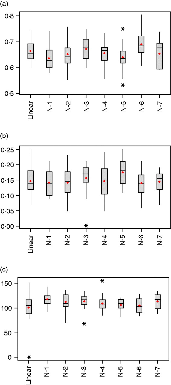
Table 1 summarizes estimated features of the network architectures used in the current study. The highest and lowest effective number of parameters were obtained for the one-neuron linear (linear-activation function in hidden and output layers) and one-neuron non-linear (tangent sigmoid activation function in hidden layer and linear activation in output layer) networks, with γ=101·1±30·3 and γ=117·3±12·5, respectively. This linear network is akin to Bayesian ridge regression, but with α and β tuned similar to the other NNs. When the number of neurons in the hidden layer was increased for non-linear networks from one to seven, γ varied between 105·6 and 117·3, but without clear differences between networks (Fig. 3 c). Even though the nominal number of parameters (n) increased from 801 to 5601, γ changed slightly only, indicating the impact of regularization.
Box-plots for (a) mean-squared error in the testing set, (b) correlation between predictions and observations in the testing set and (c) effective number of parameters, γ, after 20 independent runs (*indicates extreme values).
Parameter estimates and their standard deviations for different network architectures (results are averages of 20 independent runs)

S, number of neurons; F, objective function; SSE, sum of squares error in the training set; SSEtest, sum of squares error in the testing set; r train(test), correlation between predictions and observations in the training(testing) set; ![]() , overall correlation between observed and predicted data; n, number of parameters; γ, effective number of parameters.
, overall correlation between observed and predicted data; n, number of parameters; γ, effective number of parameters.
As shown in Table 1 and Fig. 3 a, values of the objective function (F) and mean squared error of prediction in the testing set were very similar across networks, with the distribution of values overruns showing considerable overlap. Networks with one and five neurons with non-linear activation functions had the smallest mean squared of error prediction, but there was no evidence that more complex networks provided better predictions than those attained by the linear model.
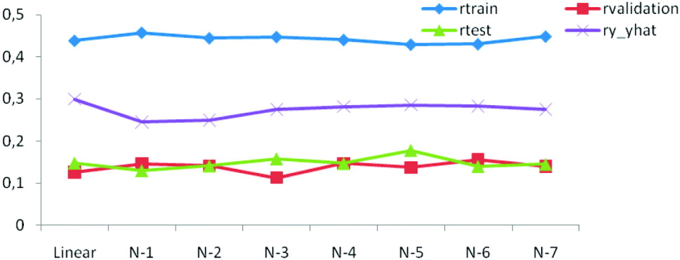
The generalization ability of the networks was also assessed by means of the correlation between predicted and observed values in the training, testing and tuning sets. As shown in Figs. 3 b and 4 the correlations were much larger in the training than in the testing and tuning sets, as expected. Predictive ability was low, and some networks did not improve over the predictive ability attained by a linear model.
Correlations between predictions and observations for training (r train), testing (r test), tuning (r validation) and overall (ry −ŷ ) for linear and seven (N-1–N-7) network architectures.
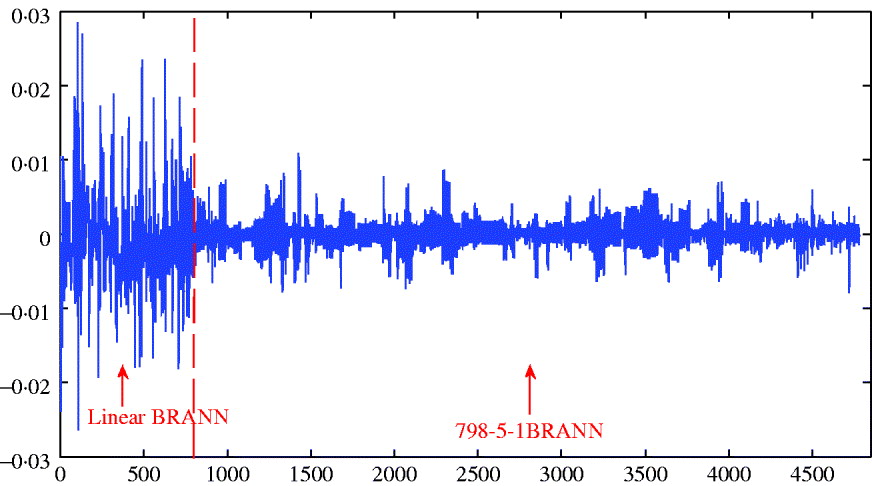
The distribution of weights in a network can also provide an indication of predictive ability; small values lead to better generalization and large weights tend to produce a more local representation. The average sum of squares of weights ranged between 0·156 and 0·196 and was smallest for the architecture with 5 neurons; this was consistent with its slightly better predictive ability. Figure 5 depicts the distributions of weights for the linear and 5-neuron architectures for the run with the largest correlation (r test=0·25 for the two networks). The weights for the linear model were larger and more variable than for the 5-neuron model.
Distribution of weights (wkj ) for the linear model and for neural network with five neurons.
(ii) Ranking SNPs for BMI
When the output layer involves a single neuron, the influence of input variables on the output is directly reflected in the weights assigned to each input, SNPs in this case. With many neurons, the influence of each SNP is more difficult to evaluate. Two different approaches for assessing the relative importance of individual SNPs in predicting BMI were considered. The relative importance of a given SNP on BMI (Joseph et al., Reference Joseph, Huang and Dickman2003) was assessed as:

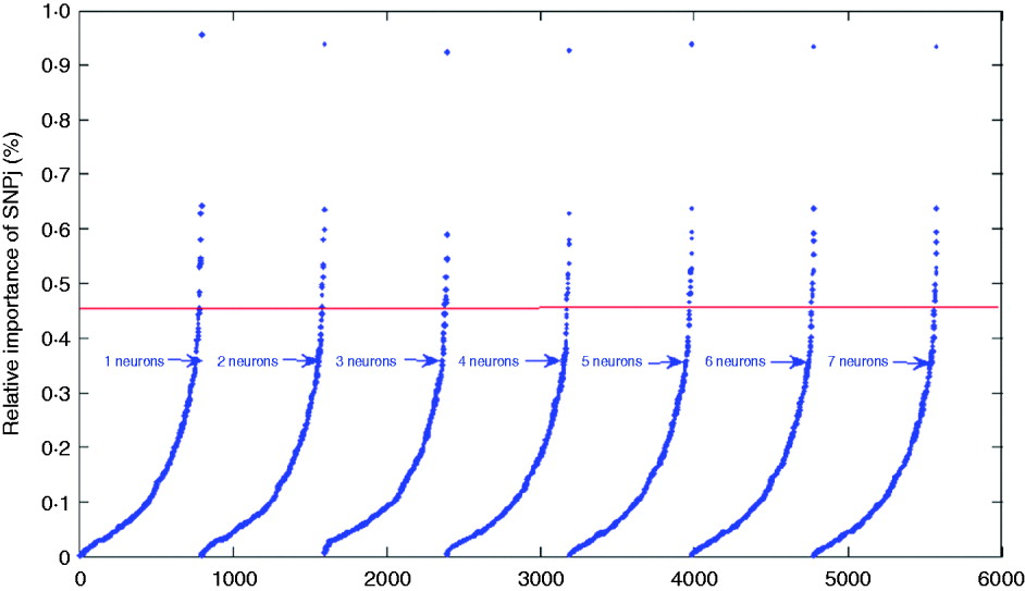
where wkj (1,1) is the connection weight from SNP j to neuron k, |.| is the absolute value function, and R and S are the number of SNPs and of hidden neurons, respectively. For indexing and ranking SNPs, data were not split into training, tuning and testing sets; rather, the whole data set was used to estimate the impact of SNPs on BMI with 1000 epochs of the algorithms run for each network. Results are shown in Table 2 and in Fig. 6 for the seven networks. Results were similar across the networks. For example, SNPs 3978, 12 132, 1096 and 2770 had the greatest impact on the networks, indicating that these SNPs may be more relevant for prediction of BMI than other SNPs. In Table 2, it is shown that SNP 3978 contributed by far the most (close to 1%) to the sum (over neurons and SNPs) of absolute values of network weights. These SNPs could be could be indicative of genomic regions associated with BMI.
Plots for the index values of 798 SNPs as prediction of BMI. The solid line gives the cutoff point separating SNPs with index values larger than 0·45%.
Relative importance of SNPs with ISNPj values larger than 0·45% for the each of the non-linear networks

Another measure used was the contribution of a given neuron, say k, to the entire network (Guha et al., Reference Guha, Stanton and Jurs2005). The bias term was taken into account, because when assessing the contribution of a given hidden neuron, all effects are relevant (Guha et al., Reference Guha, Stanton and Jurs2005). The contribution of the kth neuron to the entire network was calculated as:
Here, bk (1) are biases in the hidden layer, wkj (1,1) are weights from the input layer to the hidden layer, and the wk (2,1) are weights from the hidden layer to the output (BMI). The relative contribution of neuron k to the network was obtained as:
As shown in Table 3 the SCN k values indicate that neurons contributed about equally in networks with 2, 4, 5, 6 and 7 neurons, whereas in the 3-neuron network, the first and third neurons were more influential than the second one. It is difficult to assign an interpretation to these results.
4. Discussion
This study explored the association between 12 320 SNPs and BMI by exploiting properties of BRANN. Data were fitted using a linear activation function in both the hidden and output layers of the networks to obtain a benchmark equivalent to Bayesian ridge regression on markers. Subsequently, different architectures were explored, including a varying number of neurons, a tangent sigmoid activation function in the hidden layer and a linear activation function in the output layer (Fig. 1). Using a sigmoidal-type function in the hidden layer and a linear transfer function in the output layer may be advantageous when it is necessary to extrapolate beyond the range of the training data (Maier & Dandy, Reference Maier and Dandy2000).
Relative contribution of the kth neuron for several neural network architectures for BMI in mice

The Levenberg–Marquardt algorithm, as implemented in MATLAB, was adopted to optimize weights and biases, because previous evaluations with networks containing a smaller number of weights indicated that it was a suitable method (Demuth et al., Reference Demuth, Beale and Hagan2009). In the training process, overfitting often occurred, leading to a loss of generalization of the predictive model. Hence, BR was adopted to avoid over-fitting and improve generalization. Bayesian methods can simultaneously optimize regularization parameters in ANNs, a process that is very laborious using cross-validation (Fernandez & Caballero, Reference Fernandez and Caballero2006).
For the networks trained with BR, we examined how the effective number of parameters γ varied with architecture. As shown in Table 1, although the total number of parameters ranged from 801 to 5601, the effective number of parameters varied only from 101 to 117, on average, illustrating the extent of regularization attained. There were minor differences in predictive ability, and the network with five neurons in the hidden layer had slightly better performance, but not significantly. Although differences were minor, this agrees with several studies (Gencay & Qi, Reference Gencay and Qi2001; Joseph et al., Reference Joseph, Huang and Dickman2003; Kumar et al., Reference Kumar, Merchant and Desai2004; Xu et al., Reference Xu, Zengi, Xu, Huang, Jiang and Sun2006), suggesting that a model with a single neuron may not provide a proper representation of the true unknown function to be predicted. Since complex models are penalized in a Bayesian approach, we were able to explore complex architectures (Sorich et al., Reference Sorich, Miners, Ross, Winker, Burden and Smith2003). While more free parameters in a model can lead to smaller data error ED (MacKay, Reference MacKay1992), monitoring training error to choose among networks is not representative of prediction error.
A useful measure of generalization is the correlation coefficient between predictions and realizations in the test data set. Here, the network with five neurons had the highest correlation in the test data set (r test=0·18), but the lowest in the training data set (r train=0·43). NNs had a performance that was similar to that attained with other procedures reported in literature. Data used in our study have already been analysed in two independent studies, one comparing genome-assisted genetic evaluation methods using BR models (Legarra et al., Reference Legarra, Robert-Granie, Manfredi and Elsen2008), and another one that compared the Bayesian LASSO with other marker-based regression models (de los Campos et al., Reference de los Campos, Hugo, Gianola, Crossa, Legarra, Manfredi, Weigel and Miguel2009). The across-family predictive ability of markers in Legarra et al. (Reference Legarra, Robert-Granie, Manfredi and Elsen2008) was 0·17 which is close to r test=0·18 obtained here with the five-neuron architecture. Further, de los Campos et al. (Reference de los Campos, Hugo, Gianola, Crossa, Legarra, Manfredi, Weigel and Miguel2009) reported a rank correlation of 0·30 between phenotypic values and genomic predictions in cross-validation. The overall correlation ![]() estimated between observed and predicted data in our study varied between 0·25 and 0·30 for different network architectures (Table 1), in agreement with de los Campos et al. (Reference de los Campos, Hugo, Gianola, Crossa, Legarra, Manfredi, Weigel and Miguel2009). It is worth noting; however, that the models in Legarra et al. (Reference Legarra, Robert-Granie, Manfredi and Elsen2008) and de los Campos et al. (Reference de los Campos, Hugo, Gianola, Crossa, Legarra, Manfredi, Weigel and Miguel2009) used all 10 946 SNP markers available in their predictions, whereas here we used only 798 pre-selected SNP markers. Moreover, the 798 SNPs used to implement the BRANN were selected in a simplistic way using single marker analyses coupled with an FDR approach. Potentially more efficient approaches for pre-selection of SNPs (e.g. Long et al., Reference Long, Gianola, Rosa, Weigel and Avendan2007; Vazquez et al., Reference Vazquez, Rosa, Weigel, de los Campos, Gianola and Allison2010) could be used and tested to improve the final prediction with BRANN.
estimated between observed and predicted data in our study varied between 0·25 and 0·30 for different network architectures (Table 1), in agreement with de los Campos et al. (Reference de los Campos, Hugo, Gianola, Crossa, Legarra, Manfredi, Weigel and Miguel2009). It is worth noting; however, that the models in Legarra et al. (Reference Legarra, Robert-Granie, Manfredi and Elsen2008) and de los Campos et al. (Reference de los Campos, Hugo, Gianola, Crossa, Legarra, Manfredi, Weigel and Miguel2009) used all 10 946 SNP markers available in their predictions, whereas here we used only 798 pre-selected SNP markers. Moreover, the 798 SNPs used to implement the BRANN were selected in a simplistic way using single marker analyses coupled with an FDR approach. Potentially more efficient approaches for pre-selection of SNPs (e.g. Long et al., Reference Long, Gianola, Rosa, Weigel and Avendan2007; Vazquez et al., Reference Vazquez, Rosa, Weigel, de los Campos, Gianola and Allison2010) could be used and tested to improve the final prediction with BRANN.
Our testing set consisted of 20% (n test=379) of the available data, and this was deemed to be large enough for assessing generalization. We observed that the variability in correlations for testing data was greater than for training data. These results are in agreement with several other studies (Aggarwal et al., Reference Aggarwal, Singh, Chandra and Puri2005; Marwala, Reference Marwala2007; Kelemen & Liang, Reference Kelemen and Liang2008; Wang et al., Reference Wang, Ji, Leung and Sum2009). At any rate, the testing set must be a representative sample of the cases to which one wants to generalize.
ANNs are often considered to be more accurate predictors than other classes of models. However, they do not provide clear information regarding how input values correlate with output values. Therefore, it is challenging to obtain effective information from a neural network. Here, exploration of an extensive pool of SNPs allowed detection of relevant SNPs in connection with BMI, as pointed out in other contexts (Fernandez & Caballero, Reference Fernandez and Caballero2006; Xu et al., Reference Xu, Zengi, Xu, Huang, Jiang and Sun2006). In our study, almost the same SNPs were found to have an impact on BMI by different networks. This is suggestive of stability of the neural network approach. The importance of neurons in the hidden layer was evaluated in this study as well. An interpretation is that hidden layer neurons are analogous to latent variables in a partial least squares model. The contribution of each hidden layer neuron to the output value of the network indicates which such neurons are most relevant and which can be neglected (Guha et al., Reference Guha, Stanton and Jurs2005).
5. Conclusions
The ability of predicting BMI in this mouse data set was low irrespective of the architecture of the NNs considered. This result is consistent with other studies of the same data set, but employing different methods. Among the networks examined, there was a slight superiority of a network with five neurons in the hidden layer. BR allowed estimating all weights, and the effective number of parameters was much lower than the nominal number. Further, several networks were consistent in flagging SNPs that were associated with BMI. It is concluded that BRANN may be at least as useful as other methods for high-dimensional genome enabled prediction, where the number of inputs (e.g. SNPs) is typically much larger than the number of cases in the sample. Finally, NNs have the potential ability of capturing non-linear relationships, which may also be useful in the study of quantitative traits under complex gene action. The data set analysed here did not allow us to corroborate this possibility.
We extend our thanks to The Wellcome Trust Centre for Human Genetics, Oxford, for making the heterogeneous stock data available at http://gscan.well.ox.ac.uk.


