


1 Introduction
It is well known that the Korteweg-de Vries (KdV) equation
 $$ \begin{align} u_t-6uu_x+u_{xxx}=0 \end{align} $$
can be presented as the compatibility condition of the Lax pair [Reference Lax29]
 $$ \begin{align} \begin{aligned} &(-\partial_{xx}+u)\varphi(x,t)=E\varphi(x,t),\\ &\varphi_t(x,t)=(4\partial_{x}-6u\partial_{x}-3u_x)\varphi(x,t), \end{aligned} \end{align} $$
where E is the spectral parameter. Based on the Lax pair formulation (1.0.2), extensive researches have been conducted on the KdV equation (1.0.1) by using the inverse scattering transform [Reference Ablowitz and Clarkson1, Reference Bilman and Trogdon7, Reference Miller and Clarke32] and Riemann-Hilbert formulation [Reference Deift, Venakides and Zhou13, Reference Egorova, Gladka, Kotlyarov and Teschl16]. One of the most notable results is the existence of a special class of localized wave solutions known as solitons. The simplest example of a single soliton solution is given by
 $$ \begin{align} u(x, t) = -2 \eta^2 \operatorname{sech}^2 ( \eta(x - 4 \eta^2 t - x_0)), \end{align} $$
where the spectral parameter is $ E = \eta ^2 $
, and
$ E = \eta ^2 $
, and $ x_0 $
is the phase parameter that determines the initial position of the soliton. In this context, the position is defined by the location of the maximum of the soliton profile. On the other hand, the KdV equation admits the periodic traveling wave solution of the form [Reference Grava, Onorato, Resitori and Baronio26, Reference Gong and Wang28]
$ x_0 $
is the phase parameter that determines the initial position of the soliton. In this context, the position is defined by the location of the maximum of the soliton profile. On the other hand, the KdV equation admits the periodic traveling wave solution of the form [Reference Grava, Onorato, Resitori and Baronio26, Reference Gong and Wang28]
 $$ \begin{align} {u(x, t)=k_3+\left(k_1-k_3\right) \mathrm{dn}^2\left(\frac{\sqrt{k_1-k_3}}{\sqrt{2} }\left(x-2(k_1+k_2+k_3) t+\frac{\phi_0}{k}\right)-K(m); m\right),} \end{align} $$
where $k_1>k_2>k_3$
,
$k_1>k_2>k_3$
, ${\mathrm {dn}}(s;m)$
is the Jacobi elliptic function and
${\mathrm {dn}}(s;m)$
is the Jacobi elliptic function and $K(m)$
is a complete elliptic integral of the first kind, that is,
$K(m)$
is a complete elliptic integral of the first kind, that is, $K(m):=\int _0^{\frac {\pi }{2}} \frac {d \vartheta }{\sqrt {1-m^2 \sin ^2 \vartheta }}$
with
$K(m):=\int _0^{\frac {\pi }{2}} \frac {d \vartheta }{\sqrt {1-m^2 \sin ^2 \vartheta }}$
with $m=\frac {k_1-k_2}{k_1-k_3}$
and
$m=\frac {k_1-k_2}{k_1-k_3}$
and $k=\pi \frac {\sqrt {k_1-k_3}}{\sqrt {2} K(m)}$
. Especially, as
$k=\pi \frac {\sqrt {k_1-k_3}}{\sqrt {2} K(m)}$
. Especially, as $k_2\to k_3$
, the periodic solution (1.0.4) degenerates into the soliton solution by the identity
$k_2\to k_3$
, the periodic solution (1.0.4) degenerates into the soliton solution by the identity $\mathrm {dn}(\bullet ;1)=\mathrm {sech}(\bullet )$
.
$\mathrm {dn}(\bullet ;1)=\mathrm {sech}(\bullet )$
.
In 1971, Zakharov [Reference Zakharov38] first introduced the concept of “soliton gas” and derived an integro-differential kinetic equation for the soliton gas by evaluating the efficient modification of the soliton velocity within a rarefied gas. Specifically, he treated solitons as “particles,” and a soliton gas can be understood as a collection of randomly distributed solitons, resembling the behavior of a gas [Reference Shurgalina and Pelinovsky36]. Forty-five years later, in 2016, Zakharov and his collaborators [Reference Dyachenko, Zakharov and Zakharov15] revisited the soliton gas for the KdV equation by using the dressing method and proposed an alternate construction of the Bargmann potentials. In particular, they formulated a Riemann-Hilbert problem (RH problem) associated with the soliton gas, given as follows:
 $$ \begin{align} \begin{aligned}\Xi^{+}(i \kappa)&=M(x,\kappa) \Xi^{-}(i \kappa), \quad \Xi^{+}(-i \kappa)=M^T(x,\kappa) \Xi^{-}(-i \kappa),\\ M(x, \kappa)&=\frac{1}{1+R_1 R_2}\left[\begin{array}{ll} 1-R_1 R_2 & 2 i R_1 e^{-2 \kappa x} \\ 2 i R_2 e^{2 \kappa x} & 1-R_1 R_2 \end{array}\right], \end{aligned} \end{align} $$
where $\Xi :\mathbb {C}\to \mathbb {C}^2$
is a vector-valued function, and
$\Xi :\mathbb {C}\to \mathbb {C}^2$
is a vector-valued function, and $\kappa \in [k_1, k_2]$
with
$\kappa \in [k_1, k_2]$
with $0<k_1<k_2$
. Although research on soliton gas began many years ago, the understanding of the properties of an interacting ensemble of large solitons and their dynamic behavior, even in the absence of randomness, remains incomplete from a mathematically precise perspective. In 2003, El [Reference El17, Reference Bonnemain, Doyon and El11] proposed a unified extension of Zakharov’s kinetic equation for the KdV dense soliton gas by considering the thermodynamic limit of KdV-Whitham equations. Subsequently, the kinetic equation for soliton gas was examined for its diverse and complex mathematical characteristics [Reference Ablowitz, Cole, El, Hoefer and Luo2, Reference El, Kamchatnov, Pavlov and Zykov19, Reference Ferapontov and Pavlov20]. In addition, Bertola et al. derived the kinetic equation for the KdV equation by using the method of genus degeneration in [Reference Bertola, Jenkins and Tovbis3]. Recently, Girotti and her collaborators [Reference Girotti, Grava, Jenkins and McLaughlin21] investigated the genus one KdV soliton gas and established an asymptotic description of soliton gas dynamics for large time by using the Deift-Zhou nonlinear steepest descent method [Reference Deift and Zhou12]. They [Reference Girotti, Grava, Jenkins, McLaughlin and Minakov22] also investigated the behaviors of a trial soliton travelling through a mKdV soliton gas and built the kinetic theory for soliton gas. For a concise relationship between the mKdV equation and KdV equation, please refer to [Reference Charlier and Lenells10]. In 2020, Nabelek gave an insightful investigation of the algebro-geometric finite gap solutions to the KdV equation [Reference Nabelek40] utilizing the primitive solution framework [Reference Dyachenko, Nabelek, Zakharov and Zakharov39, Reference Dyachenko, Zakharov and Zakharov41] for the general case of “N bands” and
$0<k_1<k_2$
. Although research on soliton gas began many years ago, the understanding of the properties of an interacting ensemble of large solitons and their dynamic behavior, even in the absence of randomness, remains incomplete from a mathematically precise perspective. In 2003, El [Reference El17, Reference Bonnemain, Doyon and El11] proposed a unified extension of Zakharov’s kinetic equation for the KdV dense soliton gas by considering the thermodynamic limit of KdV-Whitham equations. Subsequently, the kinetic equation for soliton gas was examined for its diverse and complex mathematical characteristics [Reference Ablowitz, Cole, El, Hoefer and Luo2, Reference El, Kamchatnov, Pavlov and Zykov19, Reference Ferapontov and Pavlov20]. In addition, Bertola et al. derived the kinetic equation for the KdV equation by using the method of genus degeneration in [Reference Bertola, Jenkins and Tovbis3]. Recently, Girotti and her collaborators [Reference Girotti, Grava, Jenkins and McLaughlin21] investigated the genus one KdV soliton gas and established an asymptotic description of soliton gas dynamics for large time by using the Deift-Zhou nonlinear steepest descent method [Reference Deift and Zhou12]. They [Reference Girotti, Grava, Jenkins, McLaughlin and Minakov22] also investigated the behaviors of a trial soliton travelling through a mKdV soliton gas and built the kinetic theory for soliton gas. For a concise relationship between the mKdV equation and KdV equation, please refer to [Reference Charlier and Lenells10]. In 2020, Nabelek gave an insightful investigation of the algebro-geometric finite gap solutions to the KdV equation [Reference Nabelek40] utilizing the primitive solution framework [Reference Dyachenko, Nabelek, Zakharov and Zakharov39, Reference Dyachenko, Zakharov and Zakharov41] for the general case of “N bands” and $R_1R_2\neq 0$
in (1.0.5). In fact, the results presented in [Reference Girotti, Grava, Jenkins and McLaughlin21, Reference Girotti, Grava, Jenkins, McLaughlin and Minakov22] represent a particular case of (1.0.5) for
$R_1R_2\neq 0$
in (1.0.5). In fact, the results presented in [Reference Girotti, Grava, Jenkins and McLaughlin21, Reference Girotti, Grava, Jenkins, McLaughlin and Minakov22] represent a particular case of (1.0.5) for $R_2=0$
, involving only two disjoint stability zones. Furthermore, the study of soliton gas for the NLS equation was examined in [Reference Bertola, Grava and Orsatti5, Reference Bertola, Grava and Orsatti6, Reference Biondini, El, Luo, Oregero and Tovbis9, Reference Tovbis and Wang33], and the relationship between periodic potentials was explored in [Reference McLaughlin and Nabelek31]. In particular, in [Reference Girotti, Grava, McLaughlin and Najnudel23], the authors investigated random configurations of soliton gases for the focusing NLS equation and established both a law of large numbers and a central limit theorem for random sets of solitons.
$R_2=0$
, involving only two disjoint stability zones. Furthermore, the study of soliton gas for the NLS equation was examined in [Reference Bertola, Grava and Orsatti5, Reference Bertola, Grava and Orsatti6, Reference Biondini, El, Luo, Oregero and Tovbis9, Reference Tovbis and Wang33], and the relationship between periodic potentials was explored in [Reference McLaughlin and Nabelek31]. In particular, in [Reference Girotti, Grava, McLaughlin and Najnudel23], the authors investigated random configurations of soliton gases for the focusing NLS equation and established both a law of large numbers and a central limit theorem for random sets of solitons.
This paper investigates the high-genus soliton gas for the KdV equation (1.0.1), focusing specifically on the genus two soliton gas potential and its long-time asymptotics. More precisely, we consider the special case of (1.0.5) with $R_1 = 0$
and
$R_1 = 0$
and $R_2 =r_2(\lambda )$
, which involves four disjoint stability zones. Suppose
$R_2 =r_2(\lambda )$
, which involves four disjoint stability zones. Suppose $0 < \eta _1 < \eta _2 < \eta _3 < \eta _4$
and let
$0 < \eta _1 < \eta _2 < \eta _3 < \eta _4$
and let $\Sigma _1 := (\eta _1, \eta _2)$
,
$\Sigma _1 := (\eta _1, \eta _2)$
, $\Sigma _2 := (-\eta _2, -\eta _1)$
,
$\Sigma _2 := (-\eta _2, -\eta _1)$
, $\Sigma _3 := (\eta _3, \eta _4)$
, and
$\Sigma _3 := (\eta _3, \eta _4)$
, and $\Sigma _4 := (-\eta _4, -\eta _3)$
, see Figure 3. Additionally, denote
$\Sigma _4 := (-\eta _4, -\eta _3)$
, see Figure 3. Additionally, denote $\Sigma _{i,\cdots ,k} = \Sigma _i \cup \cdots \cup \Sigma _k$
. Let
$\Sigma _{i,\cdots ,k} = \Sigma _i \cup \cdots \cup \Sigma _k$
. Let $\theta (x,t;\lambda ):=x\lambda +4 t\lambda ^3$
, and then construct the following RH problem for the vector-valued function
$\theta (x,t;\lambda ):=x\lambda +4 t\lambda ^3$
, and then construct the following RH problem for the vector-valued function $X(\lambda )$
as
$X(\lambda )$
as
 $$ \begin{align} \begin{aligned} X_+(\lambda)=X_-(\lambda) \begin{cases} \begin{aligned} &\begin{pmatrix} 1 & -2ir_2(\lambda)e^{-2 i\theta(x,t;\lambda)}\\ 0 & 1 \end{pmatrix},&&\lambda\in i\Sigma_{1,3},\\ &\begin{pmatrix} 1 & 0\\ 2ir_2(\lambda)e^{2 i \theta(x,t;\lambda)} & 1 \end{pmatrix},&&\lambda\in i\Sigma_{2,4}, \end{aligned} \end{cases} \end{aligned} \end{align} $$
 $$ \begin{align} X(\lambda)\to \begin{pmatrix} 1 & 1 \end{pmatrix},\quad \lambda\to\infty, \end{align} $$
 $$ \begin{align} X(-\lambda)=X(\lambda)\begin{pmatrix} 0 & 1\\ 1 & 0 \end{pmatrix}. \end{align} $$
Then the genus two soliton gas potential of the KdV equation (1.0.1) is given by the reconstruction formula
 $$ \begin{align} u(x) = 2 \frac{\mathrm{d}}{\mathrm{d} x} \left( \lim_{\lambda \to \infty} \frac{\lambda}{i} \left(X_1(\lambda) - 1\right) \right), \end{align} $$
where $X_1(\lambda )$
is the first component of
$X_1(\lambda )$
is the first component of $X(\lambda )$
.
$X(\lambda )$
.
In what follows, we propose the main results of this work.
1.1 Statement of the main results
Firstly, a genus two KdV soliton gas potential (1.0.9) is constructed by formulating the Riemann-Hilbert problem (1.0.6)-(1.0.8) from the pure N-soliton Riemann-Hilbert problem in Section 2 for $N \to +\infty $
, where the initial positions of the N solitons are located on the positive real axis. Then, in Section 3, we establish the large x behaviors of this soliton gas potential in equation (1.1.1).
$N \to +\infty $
, where the initial positions of the N solitons are located on the positive real axis. Then, in Section 3, we establish the large x behaviors of this soliton gas potential in equation (1.1.1).
Theorem 1.1. The potential function $u(x,0)$
, which satisfies the reconstruction formula (1.0.9) and the Riemann-Hilbert problem (1.0.6)-(1.0.8), exhibits the following asymptotic behaviors:
$u(x,0)$
, which satisfies the reconstruction formula (1.0.9) and the Riemann-Hilbert problem (1.0.6)-(1.0.8), exhibits the following asymptotic behaviors:
 $$ \begin{align} u(x,0)=\begin{cases} \begin{aligned} &-\left(2\alpha+{\sum_{j=1}^4\eta_j^2}+2\partial_x^2\log\left(\Theta\left(\frac{\Omega}{2\pi i};\hat\tau\right)\right)\right)+\mathcal{O}\left(\frac{1}{x}\right),&& x\to+\infty,\\ &\mathcal{O}(e^{-c|x|}),&& x\to-\infty. \end{aligned} \end{cases} \end{align} $$
Here, $\Theta (\bullet ;\hat {\tau })$
denotes the two-phase Riemann-Theta function defined by (3.1.3),
$\Theta (\bullet ;\hat {\tau })$
denotes the two-phase Riemann-Theta function defined by (3.1.3), $\Omega $
is a two-dimensional column vector given by (3.1.5) and the imaginary part of the period matrix
$\Omega $
is a two-dimensional column vector given by (3.1.5) and the imaginary part of the period matrix $\hat {\tau }$
, as defined in (3.2.4), is positive definite. Furthermore, the parameter
$\hat {\tau }$
, as defined in (3.2.4), is positive definite. Furthermore, the parameter $\alpha $
is defined in Remark 3.1, and c is a fixed positive constant.
$\alpha $
is defined in Remark 3.1, and c is a fixed positive constant.
Indeed, the initial configuration can be regarded as a Riemann problem for the KdV condensate [Reference Congy, El, Roberti and Hoefer24], while the Riemann problem for the NLS equation has been studied in [Reference Wang and Yan34]. In [Reference Congy, El, Roberti and Hoefer24], Congy et al. studied the case involving a transition between genus $0$
and genus
$0$
and genus $1$
. In our case, the problem can be interpreted as a generalized rarefaction scenario. Figure 1 presents a direct numerical simulation of the KdV equation (1.0.1) with initial potential behaving the asymptotics in equation (1.1.1) with parameters
$1$
. In our case, the problem can be interpreted as a generalized rarefaction scenario. Figure 1 presents a direct numerical simulation of the KdV equation (1.0.1) with initial potential behaving the asymptotics in equation (1.1.1) with parameters $\eta _1 = 0.8$
,
$\eta _1 = 0.8$
, $\eta _2 = 1.2$
,
$\eta _2 = 1.2$
, $\eta _3 = 1.6$
,
$\eta _3 = 1.6$
, $\eta _4 = 2$
, and
$\eta _4 = 2$
, and $ r_2(\lambda ) = 1$
. The Figure 1 clearly shows that the plane is divided into five distinct regions, which from left to right are quiescent region, modulated one-phase wave region, unmodulated one-phase wave region, modulated two-phase wave region, and unmodulated two-phase wave region.
$ r_2(\lambda ) = 1$
. The Figure 1 clearly shows that the plane is divided into five distinct regions, which from left to right are quiescent region, modulated one-phase wave region, unmodulated one-phase wave region, modulated two-phase wave region, and unmodulated two-phase wave region.

Figure 1. The evolution of the genus two soliton gas potential of the KdV equation at $ t = 10 $
for parameters
$ t = 10 $
for parameters $\eta _1 = 0.8$
,
$\eta _1 = 0.8$
, $\eta _2 = 1.2$
,
$\eta _2 = 1.2$
, $\eta _3 = 1.6$
,
$\eta _3 = 1.6$
, $\eta _4 = 2$
, and
$\eta _4 = 2$
, and $ r_2(\lambda ) = 1 $
. The horizontal axis represents
$ r_2(\lambda ) = 1 $
. The horizontal axis represents $\frac {x}{4t}$
, and the critical points
$\frac {x}{4t}$
, and the critical points $\eta _1^2$
and
$\eta _1^2$
and $\xi _{\text {crit}}^{(j)}$
for
$\xi _{\text {crit}}^{(j)}$
for $ j = 1, 2, 3 $
partition the plane into five distinct regions. These critical values,
$ j = 1, 2, 3 $
partition the plane into five distinct regions. These critical values, $\xi _{\text {crit}}^{(j)}$
, can be calculated by using equations (4.3.13) and (4.1.12) approximately. For the given parameters, the approximate values are
$\xi _{\text {crit}}^{(j)}$
, can be calculated by using equations (4.3.13) and (4.1.12) approximately. For the given parameters, the approximate values are $\xi _{\text {crit}}^{(1)} \approx 2.0905$
,
$\xi _{\text {crit}}^{(1)} \approx 2.0905$
, $\xi _{\text {crit}}^{(2)} \approx 3.2338$
, and
$\xi _{\text {crit}}^{(2)} \approx 3.2338$
, and $\xi _{\text {crit}}^{(3)} \approx 5.8561$
.
$\xi _{\text {crit}}^{(3)} \approx 5.8561$
.
More precisely, the long-time asymptotics of $ u(x,t) $
for the genus two KdV soliton gas potential depends on the parameter
$ u(x,t) $
for the genus two KdV soliton gas potential depends on the parameter $\xi := \frac {x}{4t}$
. There are four critical values, that is,
$\xi := \frac {x}{4t}$
. There are four critical values, that is, $\eta _1^2$
and
$\eta _1^2$
and $\xi _{\text {crit}}^{(j)}$
for
$\xi _{\text {crit}}^{(j)}$
for $ j = 1, 2, 3 $
, defined in equations (4.1.12) and (4.3.13), which serve as the boundaries between different regions, as illustrated in Figure 2 and Theorem 1.2 below. The proof of Theorem 1.2 will be provided in detail in Section 4.
$ j = 1, 2, 3 $
, defined in equations (4.1.12) and (4.3.13), which serve as the boundaries between different regions, as illustrated in Figure 2 and Theorem 1.2 below. The proof of Theorem 1.2 will be provided in detail in Section 4.

Figure 2. Five asymptotic regions of the genus two KdV soliton gas potential in the x-t half plane.
Theorem 1.2. As $ t \to +\infty $
, the global long-time asymptotic behaviors of
$ t \to +\infty $
, the global long-time asymptotic behaviors of $ u(x,t) $
for the KdV equation with initial potential behaving the asymptotics in equation (1.1.1) can be described as follows:
$ u(x,t) $
for the KdV equation with initial potential behaving the asymptotics in equation (1.1.1) can be described as follows:
-
1. For fixed $\xi < \eta _1^2$
, there exists a positive constant
$ c $
such that
$$\begin{align*}u(x, t) = \mathcal{O}\left(e^{-c t}\right). \end{align*}$$
$\xi < \eta _1^2$
, there exists a positive constant
$ c $
such that
$$\begin{align*}u(x, t) = \mathcal{O}\left(e^{-c t}\right). \end{align*}$$
-
2. For
$\eta _1^2 < \xi < \xi _{\text {crit}}^{(1)}$
, the long-time asymptotics of
$u(x,t)$
can be described by a Jacobi elliptic function “
$\mathrm {dn}$
” with modulated parameter
$\alpha _1\in (\eta _1,\eta _2)$
and modulated modulus
$m_{\alpha _1} = \frac {\eta _1}{\alpha _1}$
as where the parameter
$$\begin{align*}u(x, t) = \alpha_1^2 - \eta_1^2 - 2\alpha_1^2 \mathrm{dn}^2\left(\alpha_1 \left(x - 2(\alpha_1^2 + \eta_1^2)t + \phi_{\alpha_1}\right) + K(m_{\alpha_1}); m_{\alpha_1} \right) + \mathcal{O}\left(\frac{1}{t}\right), \end{align*}$$
$\alpha _1$
is determined by equation (4.1.8), and with
$$\begin{align*}\phi_{\alpha_1} = \int_{\alpha_1}^{\eta_1} \frac{\log r(\zeta)}{R_{\alpha_1,+}(\zeta)} \frac{d\zeta}{\pi i}, \end{align*}$$
$ R_{\alpha _1}(\lambda ) := \sqrt {(\lambda ^2 - \eta _1^2)(\lambda ^2 - \alpha _1^2)} $
, where
$ R_{\alpha _1,+}(\lambda ) $
denotes the left boundary of
$ R_{\alpha _1}(\lambda )$
along the branch cuts
$(\eta _1,\eta _2)$
and
$(-\eta _2,-\eta _1)$
.
$ K(m_{\alpha _1}) $
is the complete elliptic integral of the first kind, defined as
$ K(m_{\alpha _1}) = \int _0^{\frac {\pi }{2}} \frac {d\vartheta }{\sqrt {1 - m_{\alpha _1}^2 \sin ^2 \vartheta }} $
.
-
3. For
$\xi _{\text {crit}}^{(1)} < \xi < \xi _{\text {crit}}^{(2)}$
, the long-time asymptotics of
$u(x,t)$
can be described by a Jacobi elliptic function “
$\mathrm {dn}$
” with constant coefficients below where
$$ \begin{align*} u(x,t)=\eta_{2}^2-\eta_{1}^2-2\eta_{2}^2 \mathrm{dn}^2\left(\eta_{2}(x-2(\eta_{2}^2+\eta_{1}^2)t+\phi_{\eta_{2}})+K(m_{\eta_{2}}); m_{\eta_{2}}\right) +\mathcal{O}\left(\frac{1}{t}\right), \end{align*} $$
$m_{\eta _{2}}=\frac {\eta _{1}}{\eta _{2}}$
, and where
$$ \begin{align*}\phi_{\eta_{2}}=\int_{\eta_{2}}^{\eta_{1}}\frac{\log r(\zeta)}{R_{\eta_{2},+}(\zeta)}\frac{d\zeta}{\pi i}, \end{align*} $$
$ R_{\eta _2}(\lambda ) $
is obtained by replacing
$ \alpha _1 $
with
$ \eta _2 $
in
$ R_{\alpha _1}(\lambda ) $
, while all other conventions remain consistent.
-
4. For
$\xi _{\text {crit}}^{(2)} < \xi < \xi _{\text {crit}}^{(3)}$
, the long-time asymptotics of
$u(x,t)$
can be described by the modulated two-phase wave (1.1.2)where the constant
$$ \begin{align} u(x, t) = -\left(2b_{\alpha_2,1} + \sum_{j=1}^3 \eta_j^2 + \alpha_2^2 + 2 \partial_x^2 \log\left(\Theta\left(\frac{\Omega_{\alpha_2}}{2\pi i}; \hat{\tau}_{\alpha_2}\right)\right)\right) + \mathcal{O}\left(\frac{1}{t}\right), \end{align} $$
$ b_{\alpha _2,1} $
is determined by equation (4.3.6), parameter
$\alpha _2$
is determined by equation (4.3.8) and the period matrix
$\hat {\tau }_{\alpha _2}$
is given in equation (4.3.23).
-
5. For fixed
$\xi _{\text {crit}}^{(3)} < \xi $
, the long-time asymptotics of
$u(x,t)$
can be described by the unmodulated two-phase wave where
$$ \begin{align*} u(x,t)=-\left(2b_{\eta_{4},1}+{\sum_{j=1}^4\eta_j^2}+2\partial_x^2\log\left(\Theta\left(\frac{\Omega_{\eta_{4}}}{2\pi i};\hat \tau_{\eta_{4}}\right)\right)\right)+\mathcal{O}\left(\frac{1}{t}\right), \end{align*} $$
$\hat \tau _{\eta _{4}}=\hat {\tau }$
in (3.2.4) and
$b_{\eta _{4}}, \Omega _{\eta _{4}}=\begin {pmatrix} {t\Omega _{\eta _{4},1}+{\Delta _{\eta _{4},1}}}&{t\Omega _{\eta _{4},0}+{\Delta _{\eta _{4},0}}} \end {pmatrix}^T$
are defined by (4.3.6) and (4.3.24), respectively.


In fact, the method for genus two KdV soliton gas can be generalized to investigate the soliton gases of arbitrary genus. In Section 5, the construction of KdV soliton gases of general genus $ \mathcal {N} $
is discussed, along with a preliminary analysis of their evolutionary properties.
$ \mathcal {N} $
is discussed, along with a preliminary analysis of their evolutionary properties.
1.2 Some remarks on Theorem 1.1 and Theorem 1.2
It will be seen that the studies of asymptotic behaviors of the genus two KdV soliton gas potential (1.0.9) are not the trivial generalization of that in the genus one KdV soliton gas potential in [Reference Girotti, Grava, Jenkins and McLaughlin21]. The leading-order term in asymptotic expression (1.1.2) also arises from the context of the small-dispersion limit of the KdV equation, as discussed in [Reference Claeys and Grava8, Reference Deift, Venakides and Zhou14]. Although the initial RH problem (1.0.6)–(1.0.8) involves four jump bands, corresponding to a genus three scenario, after applying the holomorphic map $ z= -\lambda ^2 $
and by using the Riemann-Hurwitz formula, the corresponding Riemann surface is indeed of genus two. Moreover, the model problem associated with this new Riemann surface resembles the one in [Reference Deift, Venakides and Zhou14], and this approach can be extended to higher-genus cases.
$ z= -\lambda ^2 $
and by using the Riemann-Hurwitz formula, the corresponding Riemann surface is indeed of genus two. Moreover, the model problem associated with this new Riemann surface resembles the one in [Reference Deift, Venakides and Zhou14], and this approach can be extended to higher-genus cases.
2 Construction of genus two KdV soliton gas potential
It is known that a pure N-soliton solution of the KdV equation (1.0.1) associates with a vector-valued RH problem. To be specific, let $M(\lambda )$
be a
$M(\lambda )$
be a $1\times 2$
vector satisfying:
$1\times 2$
vector satisfying:
(i) $M(\lambda )$
is meromorphic in the whole complex plane, with simple poles at
$M(\lambda )$
is meromorphic in the whole complex plane, with simple poles at $\left \{\lambda _j\right \}_{j=1}^N$
in
$\left \{\lambda _j\right \}_{j=1}^N$
in $i \mathbb {R}_{+}$
and the corresponding conjugate points
$i \mathbb {R}_{+}$
and the corresponding conjugate points $\left \{\bar {\lambda }_j\right \}_{j=1}^N$
in
$\left \{\bar {\lambda }_j\right \}_{j=1}^N$
in $i \mathbb {R}_{-}$
;
$i \mathbb {R}_{-}$
;
(ii) The following residue conditions for $M(\lambda )$
hold
$M(\lambda )$
hold
 $$ \begin{align*} \underset{\lambda=\lambda_j}{\operatorname{res}} M(\lambda)=\lim _{\lambda \rightarrow \lambda_j} M(\lambda) \begin{pmatrix} 0 & \frac{c_j e^{-2 i \theta(x,t;\lambda)}}{N} \\ 0 & 0 \end{pmatrix} , \quad \underset{\lambda=\bar\lambda_j}{\operatorname{res}} M(\lambda)=\lim _{\lambda \rightarrow \bar{\lambda}_j} M(\lambda)\begin{pmatrix} 0 & 0\\ \frac{-c_j e^{2 i \theta(x,t;\lambda)}}{N} & 0 \end{pmatrix}, \end{align*} $$
where $c_j \in i \mathbb {R}_{+}, j=1,\cdots ,N$
and
$c_j \in i \mathbb {R}_{+}, j=1,\cdots ,N$
and $\theta (x,t;\lambda )=x\lambda +4t\lambda ^3$
.
$\theta (x,t;\lambda )=x\lambda +4t\lambda ^3$
.
(iii) $M(\lambda )$
satisfies the asymptotics
$M(\lambda )$
satisfies the asymptotics $M(\lambda )= \begin {pmatrix} 1 & 1 \end {pmatrix}+\mathcal {O}\left (\frac {1}{\lambda }\right )$
for
$M(\lambda )= \begin {pmatrix} 1 & 1 \end {pmatrix}+\mathcal {O}\left (\frac {1}{\lambda }\right )$
for $\lambda \rightarrow \infty $
;
$\lambda \rightarrow \infty $
;
(iv) M admits the symmetry
 $$ \begin{align*} M(-\lambda)=M(\lambda)\left(\begin{array}{ll} 0 & 1 \\ 1 & 0 \end{array}\right). \end{align*} $$
The stationary N-soliton solution of the KdV equation (1.0.1) is constructed by
 $$ \begin{align*} u(x,t)=2 \frac{\mathrm{d}}{\mathrm{d} x}\left(\lim _{\lambda \rightarrow \infty} \frac{\lambda}{i}\left(M_1(\lambda)-1\right)\right), \end{align*} $$
where $M_1(\lambda )$
is the first element of row vector
$M_1(\lambda )$
is the first element of row vector $M(\lambda )$
. Specially, for
$M(\lambda )$
. Specially, for $N=1$
and taking
$N=1$
and taking $\lambda _1=i\eta , c_1=ic,c>0$
, the stationary one-soliton solution of the KdV equation (1.0.1) is derived as
$\lambda _1=i\eta , c_1=ic,c>0$
, the stationary one-soliton solution of the KdV equation (1.0.1) is derived as
 $$ \begin{align*} u(x,t)=-2 \eta^2 \operatorname{sech}^2\left( \eta\left(x-4\eta^2t-x_0\right)\right), \end{align*} $$
which is a time-independent version of the single soliton solution (1.0.3) with initial position
 $$ \begin{align*} x_0=\frac{1}{2\eta}\log\frac{2\eta}{c}\in\mathbb R. \end{align*} $$
Reminding the notations $\Sigma _j~(j=1,2,3,4)$
above, for the sake of simplicity, when considering
$\Sigma _j~(j=1,2,3,4)$
above, for the sake of simplicity, when considering $N\to +\infty $
restricted on the four bands
$N\to +\infty $
restricted on the four bands $(i\eta _1,i\eta _2), (i\eta _3,i\eta _4), (-i\eta _2, -i\eta _1)$
and
$(i\eta _1,i\eta _2), (i\eta _3,i\eta _4), (-i\eta _2, -i\eta _1)$
and $(-i\eta _4, -i\eta _3)$
respectively, we take the following assumptions.
$(-i\eta _4, -i\eta _3)$
respectively, we take the following assumptions.
Assumption 1. Assume the next three items hold:
-
1. Divide
$\{\lambda _j\}_{j=1}^N$
into two parts, that are
$\{\lambda _l\}_{l=1}^{N_1}$
and
$\{\lambda _k\}_{k=1}^{N_2}$
, with
$N_1+N_2=N$
. Suppose the
$N_1$
poles are uniformly distributed on
$(i \eta _1,i\eta _2)$
, while the
$N_2$
poles are uniformly distributed on
$(i \eta _3,i\eta _4)$
. More explicitly, let
$|\lambda _{l+1}-\lambda _{l}|=\frac {\eta _2-\eta _1}{N_1}$
and
$|\lambda _{k+1}-\lambda _{k}|=\frac {\eta _4-\eta _3}{N_2}$
. -
2. Similarly, the coefficients
$c_j$
are also divided into two groups, that is,
$\{c_l\}_{l=1}^{N_1},\{c_k\}_{k=1}^{N_2}$
, and are purely imaginary. Moreover, assume that where
$$ \begin{align*} c_l&=\frac{i(\eta_2-\eta_1)r_2(\lambda_l)}{\pi},~l=1,2,\cdots,N_1,\\ c_k&=\frac{i(\eta_4-\eta_3)r_2(\lambda_k)}{\pi},~k=1,2,\cdots,N_2, \end{align*} $$
$r_2(\lambda )$
is an analytic function for
$\lambda $
near
$i\Sigma _{1,2,3,4}$
, with symmetry
$r_2(\bar \lambda )=r_2(\lambda )$
. Moreover,
$r_2(\lambda )$
is assumed to be a real-valued positive nonvanishing function for
$\lambda $
in the closure of
$\Sigma _{1,2,3,4}$
.
-
3. Indeed, we only consider the case that
$N_1\to +\infty $
and
$N_2\to +\infty $
, simultaneously.


Note that the corresponding conjugate points $\left \{\bar {\lambda }_j\right \}_{j=1}^N$
are considered in the same way on
$\left \{\bar {\lambda }_j\right \}_{j=1}^N$
are considered in the same way on $(-i\eta _2, -i\eta _1)$
and
$(-i\eta _2, -i\eta _1)$
and $(-i\eta _4, -i\eta _3)$
. Now, remove the poles in
$(-i\eta _4, -i\eta _3)$
. Now, remove the poles in $M(\lambda )$
by taking the transformations
$M(\lambda )$
by taking the transformations
 $$ \begin{align*} Z(\lambda)=\begin{cases} \begin{aligned} &M(\lambda) \begin{pmatrix} 1 & -\frac{1}{N}\sum_{j=1}^{N}\frac{c_j e^{-2 i {\theta(x,t;\lambda)}}}{\lambda-\lambda_j} \\ 0 & 1 \end{pmatrix},&&\lambda\ \text{within}\ \gamma_+,\\ &M(\lambda) \begin{pmatrix} 1 & 0 \\ \frac{1}{N}\sum_{j=1}^{N}\frac{c_j e^{{2 i \theta(x,t;\lambda)}}}{\lambda+\lambda_j} & 1 \end{pmatrix},&&\lambda\ \text{within}\ \gamma_-, \end{aligned} \end{cases} \end{align*} $$
where $\gamma _+$
is a counter clockwise contour, which surrounds the interval
$\gamma _+$
is a counter clockwise contour, which surrounds the interval $(i\eta _1,i\eta _2)$
and
$(i\eta _1,i\eta _2)$
and $(i\eta _3,i\eta _4)$
in the upper half plane, and
$(i\eta _3,i\eta _4)$
in the upper half plane, and $\gamma _-$
is a clockwise contour, which surrounds the interval
$\gamma _-$
is a clockwise contour, which surrounds the interval $(-i\eta _2,-i\eta _1)$
and
$(-i\eta _2,-i\eta _1)$
and $(-i\eta _4,-i\eta _3)$
in the lower half plane. Consequently, the jump conditions for function
$(-i\eta _4,-i\eta _3)$
in the lower half plane. Consequently, the jump conditions for function $Z(\lambda )$
are converted into
$Z(\lambda )$
are converted into
 $$ \begin{align*} Z_+(\lambda)=Z_-(\lambda)\begin{cases} \begin{aligned} &\begin{pmatrix} 1 & -\frac{1}{N}\sum_{j=1}^{N}\frac{c_j e^{-2 i{ \theta(x,t;\lambda)}}}{\lambda-\lambda_j} \\ 0 & 1 \end{pmatrix}, &&\lambda\in\gamma_+,\\ &\begin{pmatrix} 1 & 0 \\ -\frac{1}{N}\sum_{j=1}^{N}\frac{c_j e^{2 i { \theta(x,t;\lambda)}}}{\lambda+\lambda_j} & 1 \end{pmatrix}, &&\lambda\in\gamma_-. \end{aligned} \end{cases} \end{align*} $$
As $N_1,N_2\to +\infty $
, one has
$N_1,N_2\to +\infty $
, one has $N=N_1+N_2\to +\infty $
. For any open set
$N=N_1+N_2\to +\infty $
. For any open set $U_{1}$
containing
$U_{1}$
containing $i\Sigma _{1}\cup i\Sigma _{3}$
, the series converges uniformly for all
$i\Sigma _{1}\cup i\Sigma _{3}$
, the series converges uniformly for all $\lambda \in \mathbb C\setminus U_1$
, that is
$\lambda \in \mathbb C\setminus U_1$
, that is
 $$ \begin{align*} \begin{aligned} \mathop{\mathrm{lim}}\limits_{N\to+\infty}\frac{1}{N}\sum_{j=1}^{N}\frac{c_j }{\lambda-\lambda_j}&= \mathop{\mathrm{ lim}}\limits_{N_1\to+\infty}\frac{1}{N_1}\sum_{l=1}^{N_1}\frac{1}{\lambda-\lambda_l}\frac{(\eta_2-\eta_1) ir_2(\lambda_l)}{\pi}+\mathop{\mathrm{lim}}\limits_{N_2\to+\infty}\frac{1}{N_2}\sum_{k=1}^{N_2}\frac{1}{\lambda-\lambda_k}\frac{(\eta_4-\eta_3)ir_2(\lambda_k)}{\pi}\\ &=\int_{i\eta_1}^{i\eta_2}\frac{2ir_2(\zeta)}{\lambda-\zeta}\frac{d\zeta}{2\pi i}+\int_{i\eta_3}^{i\eta_4}\frac{2ir_2(\zeta)}{\lambda-\zeta}\frac{d\zeta}{2\pi i}. \end{aligned} \end{align*} $$
Similarly, for any open set $U_{2}$
containing
$U_{2}$
containing $i\Sigma _{2}\cup i\Sigma _{4}$
, the series converges uniformly for all
$i\Sigma _{2}\cup i\Sigma _{4}$
, the series converges uniformly for all $\lambda \in \mathbb C\setminus U_2$
, that is
$\lambda \in \mathbb C\setminus U_2$
, that is
 $$ \begin{align*} \mathop{\mathrm{lim}}\limits_{N\to+\infty}\frac{1}{N}\sum_{j=1}^{N}\frac{c_j }{\lambda+\lambda_j}=\int_{-i\eta_2}^{-i\eta_1}\frac{2ir_2(\zeta)}{\zeta-\lambda}\frac{d\zeta}{2\pi i}+\int_{-i\eta_4}^{-i\eta_3}\frac{2ir_2(\zeta)}{\zeta-\lambda}\frac{d\zeta}{2\pi i}. \end{align*} $$
As result, a limiting RH problem for $Z(\lambda )$
is obtained below
$Z(\lambda )$
is obtained below
 $$ \begin{align*} Z_+(\lambda)=Z_-(\lambda)\begin{cases} \begin{aligned} &\begin{pmatrix} 1 & e^{-2i{ \theta(x,t;\lambda)}}(\int_{i\eta_1}^{i\eta_2}\frac{2ir_2(\zeta)}{\zeta-\lambda}\frac{d\zeta}{2\pi i}+\int_{i\eta_3}^{i\eta_4}\frac{2ir_2(\zeta)}{\zeta-\lambda}\frac{d\zeta}{2\pi i})\\ 0 & 1 \end{pmatrix},&&\lambda\in\gamma_+,\\ &\begin{pmatrix} 1 & 0\\ e^{2i{ \theta(x,t;\lambda)}}(\int_{-i\eta_2}^{-i\eta_1}\frac{2ir_2(\zeta)}{\zeta-\lambda}\frac{d\zeta}{2\pi i}+\int_{-i\eta_4}^{-i\eta_3}\frac{2ir_2(\zeta)}{\zeta-\lambda}\frac{d\zeta}{2\pi i}) & 1 \end{pmatrix},&&\lambda\in\gamma_-,\\ \end{aligned} \end{cases} \end{align*} $$
 $$ \begin{align*}Z(\lambda)= \begin{pmatrix} 1 & 1 \end{pmatrix}+\mathcal{O}\left(\frac{1}{\lambda}\right),\quad \text{for}\quad \lambda \to \infty.\end{align*} $$
Now, comparing the jump conditions of $Z(\lambda )$
on the contour
$Z(\lambda )$
on the contour $\gamma _{\pm }$
into jumps on
$\gamma _{\pm }$
into jumps on $\Sigma _{1,2,3,4}$
by defining
$\Sigma _{1,2,3,4}$
by defining
 $$ \begin{align*} X(\lambda)= \begin{cases} \begin{aligned} &Z(\lambda)\begin{pmatrix} 1 & -e^{-2i{ \theta(x,t;\lambda)}}(\int_{i\eta_1}^{i\eta_2}\frac{2ir_2(\zeta)}{\zeta-\lambda}\frac{d\zeta}{2\pi i}+\int_{i\eta_3}^{i\eta_4}\frac{2ir_2(\zeta)}{\zeta-\lambda}\frac{d\zeta}{2\pi i})\\ 0 & 1 \end{pmatrix},&& \lambda\ \text{within}\ \gamma_+,\\ &Z(\lambda)\begin{pmatrix} 1 & 0\\ e^{2i{ \theta(x,t;\lambda)}}(\int_{-i\eta_2}^{-i\eta_1}\frac{2ir_2(\zeta)}{\zeta-\lambda}\frac{d\zeta}{2\pi i}+\int_{-i\eta_4}^{-i\eta_3}\frac{2ir_2(\zeta)}{\zeta-\lambda}\frac{d\zeta}{2\pi i}) & 1 \end{pmatrix},&& \lambda\ \text{within}\ \gamma_-,\\ &Z(\lambda), && \lambda\ \text{outside}\ \gamma_{\pm}. \end{aligned} \end{cases} \end{align*} $$
By using the Plemelj formula, the RH problem for function $X(\lambda )$
in (1.0.6)–(1.0.8) is derived immediately. Finally, transform the RH problem on contours
$X(\lambda )$
in (1.0.6)–(1.0.8) is derived immediately. Finally, transform the RH problem on contours $i\Sigma _{1,2,3,4}$
into that on contours
$i\Sigma _{1,2,3,4}$
into that on contours $\Sigma _{1,2,3,4}$
by defining
$\Sigma _{1,2,3,4}$
by defining $Y(\lambda )=X(i\lambda ),\ r(\lambda )=2r_2(i\lambda )$
, then we arrive at the RH problem for the soliton gas potential of the KdV equation as follows.
$Y(\lambda )=X(i\lambda ),\ r(\lambda )=2r_2(i\lambda )$
, then we arrive at the RH problem for the soliton gas potential of the KdV equation as follows.
The function $Y(\lambda )$
is analytic for
$Y(\lambda )$
is analytic for $\lambda \in \mathbb {C} \setminus \Sigma _{1,2,3,4}$
with
$\lambda \in \mathbb {C} \setminus \Sigma _{1,2,3,4}$
with $\Sigma _{1,2,3,4}:=\Sigma _1\cup \Sigma _2\cup \Sigma _3\cup \Sigma _4$
, see Figure 3, and has the properties:
$\Sigma _{1,2,3,4}:=\Sigma _1\cup \Sigma _2\cup \Sigma _3\cup \Sigma _4$
, see Figure 3, and has the properties:
 $$ \begin{align*} Y_{+}( \lambda)=Y_{-}( \lambda) \begin{cases}{\left(\begin{array}{cc} 1 & -i r( \lambda) e^{{2 \lambda x-8\lambda^3t}} \\ 0 & 1 \end{array}\right)}, & \lambda \in \Sigma_{1,3}, \\ {\left(\begin{array}{cc} 1 & 0 \\ i r( \lambda) e^{{-2 \lambda x+8\lambda^3t}} & 1 \end{array}\right)}, & \lambda \in \Sigma_{2,4},\end{cases} \end{align*} $$
 $$ \begin{align*} Y(\lambda)=(1\quad 1)+\mathcal{O}\left(\frac{1}{\lambda}\right), \end{align*} $$
 $$ \begin{align*} Y(-\lambda)=Y(\lambda)\left(\begin{matrix} 0&1\\ 1&0 \end{matrix}\right). \end{align*} $$

Figure 3. The jump contour for $ Y(\lambda ) $
and the associated jump matrices.
$ Y(\lambda ) $
and the associated jump matrices.
So the KdV soliton gas potential can be reformulated by
 $$ \begin{align*} u(x,t)=2 \frac{\mathrm{d}}{\mathrm{d} x}\left(\lim _{\lambda \rightarrow \infty} {\lambda}\left(Y_1(\lambda )-1\right)\right), \end{align*} $$
where $Y_1(\lambda )$
is the first component of vector-valued function
$Y_1(\lambda )$
is the first component of vector-valued function $Y(\lambda )$
.
$Y(\lambda )$
.
Lemma 2.1. The solution to the RH problem concerning row vector $Y(\lambda )$
stated above exists and is unique.
$Y(\lambda )$
stated above exists and is unique.
Proof. Rewrite row vector $Y(\lambda )$
as
$Y(\lambda )$
as $(y^{(1)}(\lambda ),y^{(2)}(\lambda ))$
. Combining the jump conditions on
$(y^{(1)}(\lambda ),y^{(2)}(\lambda ))$
. Combining the jump conditions on $\Sigma _{2,4}$
, it is deduced that
$\Sigma _{2,4}$
, it is deduced that
 $$ \begin{align*} y^{(1)}_+(\lambda)=y^{(1)}_-(\lambda)-ir(\lambda)y^{(2)}_+(\lambda),\quad y^{(2)}_+(\lambda)=y^{(2)}_-(\lambda). \end{align*} $$
It is evident that $y^{(2)}(\lambda )$
is holomorphic across
$y^{(2)}(\lambda )$
is holomorphic across $\Sigma _{2,4}$
, while
$\Sigma _{2,4}$
, while $y^{(1)}(\lambda )$
satisfies an inhomogeneous scalar RH problem. For convenience, denote
$y^{(1)}(\lambda )$
satisfies an inhomogeneous scalar RH problem. For convenience, denote $f(\lambda ):=-i\sqrt {r(\lambda )}y^{(2)}(\lambda )$
. As a result, the solution for
$f(\lambda ):=-i\sqrt {r(\lambda )}y^{(2)}(\lambda )$
. As a result, the solution for $y^{(1)}(\lambda )$
can be represented as
$y^{(1)}(\lambda )$
can be represented as
 $$ \begin{align*} y^{(1)}(\lambda)=1+\frac{1}{2\pi i}\int_{\Sigma_{2,4}}\frac{\sqrt{r(s)}f(s)}{s-\lambda}ds. \end{align*} $$
Moreover, the symmetry of $Y(\lambda )$
implies that
$Y(\lambda )$
implies that $y^{(1)}(-\lambda )=y^{(2)}(\lambda )$
, which shows that
$y^{(1)}(-\lambda )=y^{(2)}(\lambda )$
, which shows that
 $$ \begin{align*} {y^{(2)}(\lambda)=1+\frac{1}{2\pi i}\int_{\Sigma_{2,4}}\frac{\sqrt{r(s)}f(s)}{s+\lambda}ds.} \end{align*} $$
Multiplying both sides of the above equation by $-i\sqrt {r(x,t;\lambda )}$
, an integral equation for
$-i\sqrt {r(x,t;\lambda )}$
, an integral equation for $f(\lambda )$
is obtained as
$f(\lambda )$
is obtained as
 $$ \begin{align*} f(\lambda)+\frac{\sqrt{r(\lambda)}}{2\pi}\int_{\Sigma_{2,4}}\frac{\sqrt{r(s)}f(s)}{s+\lambda}ds =-i\sqrt{r(\lambda)}, \end{align*} $$
which is equivalent to $(I+T)f=b$
, where
$(I+T)f=b$
, where $T=\frac {\sqrt {r(x,t;\lambda )}}{2\pi }\int _{\Sigma _{2,4}}\frac {\sqrt {r(x,t;s)}}{s+\lambda }ds$
and
$T=\frac {\sqrt {r(x,t;\lambda )}}{2\pi }\int _{\Sigma _{2,4}}\frac {\sqrt {r(x,t;s)}}{s+\lambda }ds$
and $b=-i\sqrt {r(\lambda )}$
. Due to the fact that the finite interval integral can be treated as a Riemann integral, it follows that the operator T is compact. Moreover, the index of
$b=-i\sqrt {r(\lambda )}$
. Due to the fact that the finite interval integral can be treated as a Riemann integral, it follows that the operator T is compact. Moreover, the index of $I+T$
is zero, that is,
$I+T$
is zero, that is, $\mathrm {Ind}(I+T)=\text {dim } N_{I+T}-\text {Codim } R_{I+T}=0$
, where
$\mathrm {Ind}(I+T)=\text {dim } N_{I+T}-\text {Codim } R_{I+T}=0$
, where $ N_{I+T} $
and
$ N_{I+T} $
and $ R_{I+T} $
denote the kernel and range of the operator
$ R_{I+T} $
denote the kernel and range of the operator $ I+T $
, respectively. It implies that
$ I+T $
, respectively. It implies that $I+T$
is an injective if and only if it is a surjective. It suffices to show that T is a positive operator, that is,
$I+T$
is an injective if and only if it is a surjective. It suffices to show that T is a positive operator, that is, $(Tx,x)\geq 0$
. This has been proven in the appendix of Ref. [Reference Girotti, Grava, Jenkins and McLaughlin21].
$(Tx,x)\geq 0$
. This has been proven in the appendix of Ref. [Reference Girotti, Grava, Jenkins and McLaughlin21].
3 The large x behaviors of the genus two KdV soliton gas potential
This section proves the Theorem 1.1, which is to examine the large x behaviors of the genus two KdV soliton gas potential constructed in Section 2.
Firstly, let $t=0$
and consider the case of
$t=0$
and consider the case of $x\to +\infty $
. To deform the RH problem associated with the genus two KdV soliton gas potential, suppose that
$x\to +\infty $
. To deform the RH problem associated with the genus two KdV soliton gas potential, suppose that $g(\lambda )$
satisfies the following scalar RH problem:
$g(\lambda )$
satisfies the following scalar RH problem:
The function $g(\lambda )$
is analytic for
$g(\lambda )$
is analytic for $\lambda \in \mathbb {C}\setminus [-\eta _4,\eta _4]$
, and
$\lambda \in \mathbb {C}\setminus [-\eta _4,\eta _4]$
, and
 $$\begin{align*}\begin{aligned} & g_+(\lambda)+g_-(\lambda)=2\lambda, && \lambda\in\Sigma_{1,2,3,4}, \\ & g_+(\lambda)-g_-(\lambda)=\Omega_0, && \lambda\in [-\eta_1,\eta_1], \\ & g_+(\lambda)-g_-(\lambda)=\Omega_1, && \lambda\in [\eta_2,\eta_3], \\ & g_+(\lambda)-g_-(\lambda)=\Omega_2, && \lambda\in [-\eta_3,-\eta_2], \\ & g(\lambda)={\mathcal{O}\left(\frac{1}{\lambda}\right),} && \lambda\to\infty, \end{aligned} \end{align*}$$
where $\Omega _{0,1,2}$
are independent of x. Moreover, the derivative of the function
$\Omega _{0,1,2}$
are independent of x. Moreover, the derivative of the function $g(\lambda )$
also satisfies a scalar RH problem of the form
$g(\lambda )$
also satisfies a scalar RH problem of the form
 $$\begin{align*}\begin{aligned} & g^{\prime}_+(\lambda)+g^{\prime}_-(\lambda)=2, && \lambda\in\Sigma_{1,2,3,4}, \\ & g^{\prime}_+(\lambda)-g^{\prime}_-(\lambda)=0, && \lambda\in [-\eta_4,\eta_4]\setminus\Sigma_{1,2,3,4}, \\ & g'(\lambda)=\mathcal{O}\left(\frac{1}{\lambda^2}\right), && \lambda\to\infty. \end{aligned} \end{align*}$$
By the uniqueness of solution to the RH problem, it can be checked that $g'(\lambda )$
is an even function.
$g'(\lambda )$
is an even function.
Introduce
 $$\begin{align*}R(\lambda)=\sqrt{(\lambda^2-\eta_1^2)(\lambda^2-\eta_2^2)(\lambda^2-\eta_3^2)(\lambda^2-\eta_4^2)}, \end{align*}$$
and assume $R_+(\lambda )$
as the upper sheet of
$R_+(\lambda )$
as the upper sheet of $R(\lambda )$
, with
$R(\lambda )$
, with $R(\lambda )\to +\infty $
as
$R(\lambda )\to +\infty $
as $\lambda \to +\infty $
, for the sake of the subsequent discussion. Define
$\lambda \to +\infty $
, for the sake of the subsequent discussion. Define
 $$\begin{align*}\begin{aligned} g'({\lambda})=1-\frac{\lambda^4+\alpha\lambda^2+\beta}{R(\lambda)}, \end{aligned} \end{align*}$$
and
 $$ \begin{align} g(\lambda)=\lambda-\int_{\eta_4}^\lambda\frac{\zeta^4+\alpha\zeta^2+\beta}{R(\zeta)}d\zeta. \end{align} $$
Moreover, introduce a two-sheeted Riemann surface of genus three as follows:
 $$ \begin{align*}\mathcal{S}=\{(\lambda,\eta)|\eta^2=(\lambda^2-\eta_1^2)(\lambda^2-\eta_2^2)(\lambda^2-\eta_3^2)(\lambda^2-\eta_4^2)\}, \end{align*} $$
which includes two infinite points $\infty _{\pm }$
to ensure the compactness of the Riemann surface. Subsequently, define the basis of cycles for Riemann surface
$\infty _{\pm }$
to ensure the compactness of the Riemann surface. Subsequently, define the basis of cycles for Riemann surface $\mathcal {S}$
shown in Figure 4.
$\mathcal {S}$
shown in Figure 4.

Figure 4. The Riemann surface $\mathcal {S}$
of genus three and its basis of circles.
$\mathcal {S}$
of genus three and its basis of circles.
The jump conditions for $g(\lambda )$
implies that for
$g(\lambda )$
implies that for $j=1,2,3$
 $$ \begin{align} \begin{aligned} & \oint_{a_j}\frac{\zeta^4+\alpha\zeta^2+\beta}{R_+(\zeta)}d\zeta=0, \ \oint_{b_1}\frac{\zeta^4+\alpha\zeta^2+\beta}{R_+(\zeta)}d\zeta=\Omega_1, \\ & \oint_{b_2}\frac{\zeta^4+\alpha\zeta^2+\beta} {R_+(\zeta)}d\zeta=\Omega_0, \ \oint_{b_3}\frac{\zeta^4+\alpha\zeta^2+\beta} {R_+(\zeta)}d\zeta=\Omega_2. \\ \end{aligned} \end{align} $$
Furthermore, it should be noted that $\frac {\zeta ^4+\alpha \zeta ^2+\beta }{R(\zeta )}d\zeta $
, denoted as
$\frac {\zeta ^4+\alpha \zeta ^2+\beta }{R(\zeta )}d\zeta $
, denoted as $\eta $
, is a second kind Abelian differential on
$\eta $
, is a second kind Abelian differential on $\mathcal {S}$
, with poles only at
$\mathcal {S}$
, with poles only at $\infty _{\pm }$
. Introduce a basis of holomorphic differential as
$\infty _{\pm }$
. Introduce a basis of holomorphic differential as
 $$ \begin{align*} {\tilde \omega}_j=\frac{\zeta^{j-1}}{R(\zeta)}d\zeta,\quad j=1,2,3, \end{align*} $$
and denote $A:=(\oint _{a_j}\tilde \omega _i)_{3\times 3}$
which is a nondegenerated matrix. According to the Riemann Bilinear relations [Reference Bertola4], one can obtain that
$A:=(\oint _{a_j}\tilde \omega _i)_{3\times 3}$
which is a nondegenerated matrix. According to the Riemann Bilinear relations [Reference Bertola4], one can obtain that
 $$ \begin{align*} \sum_{j=1}^3\oint_{a_j}\tilde \omega^i\oint_{b_j}\eta=-{2i\pi}\sum_{p=\infty_{\pm}}\mathrm{res}_{p}\frac{\tilde \omega_i}{\lambda},i=1,2,3, \end{align*} $$
that is,
 $$ \begin{align} \begin{aligned} &\Omega_1\int_{a_1}\tilde\omega_1+\Omega_0\int_{a_2}\tilde\omega_1+\Omega_2\int_{a_3}\tilde\omega_1=0,\\ &\Omega_1\int_{a_1}\tilde\omega_2+\Omega_0\int_{a_2}\tilde\omega_2+\Omega_2\int_{a_3}\tilde\omega_2=0,\\ &\Omega_1\int_{a_1}\tilde\omega_3+\Omega_0\int_{a_2}\tilde\omega_3+\Omega_2\int_{a_3}\tilde\omega_3=4\pi i.\\ \end{aligned} \end{align} $$
Consequently, the quantities $\Omega _0$
,
$\Omega _0$
, $\Omega _1$
and
$\Omega _1$
and $\Omega _2$
can be expressed by
$\Omega _2$
can be expressed by
 $$ \begin{align*} \Omega_1=4\pi i(A^{-1})_{13},\ \Omega_0=4\pi i(A^{-1})_{23},\ \Omega_2=4\pi i(A^{-1})_{33}. \end{align*} $$
Remark 3.1. Since $\zeta /{R(\zeta )}$
is odd, and
$\zeta /{R(\zeta )}$
is odd, and $1/{R(\zeta )}$
and
$1/{R(\zeta )}$
and $\zeta ^2/{R(\zeta )}$
are even, it follows that
$\zeta ^2/{R(\zeta )}$
are even, it follows that $A_{13}=A_{11}$
and
$A_{13}=A_{11}$
and $A_{22}=0$
, which implies that
$A_{22}=0$
, which implies that $(A^{-1})_{13}=(A^{-1})_{33}$
, that is,
$(A^{-1})_{13}=(A^{-1})_{33}$
, that is, $\Omega _1=\Omega _2$
. Alternatively, by using the equalities for
$\Omega _1=\Omega _2$
. Alternatively, by using the equalities for $j=1,2$
below
$j=1,2$
below
 $$ \begin{align*} \oint_{a_j}\frac{\zeta^4+\alpha\zeta^2+\beta}{R(\zeta)}d\zeta=0, \end{align*} $$
the parameters $\alpha $
and
$\alpha $
and $\beta $
can be determined immediately.
$\beta $
can be determined immediately.
Now, we are ready to deform the RH problem. To do so, take the transformation
 $$ \begin{align*} T(\lambda)=Y(\lambda)e^{xg(\lambda)\sigma_3}f(\lambda)^{\sigma_3}, \end{align*} $$
where $f(\lambda )$
is a function to be determined and
$f(\lambda )$
is a function to be determined and $T(\lambda )$
satisfies the RH problem:
$T(\lambda )$
satisfies the RH problem:
 $$ \begin{align*} \begin{aligned} & T_{+}(\lambda)=T_{-}(\lambda) V(\lambda) \\ & V(\lambda)= \begin{cases} \begin{aligned} &\left(\begin{array}{cc} e^{x(g_{+}(\lambda)-g_{-}(\lambda))} \frac{f_{+}(\lambda)}{f_{-}(\lambda)} & \frac{-i r(\lambda)}{f_{+}(\lambda) f_{-}(\lambda)} \\ 0 & e^{-x(g_{+}(\lambda)-g_{-}(\lambda))} \frac{f_{-}(\lambda)}{f_{+}(\lambda)} \end{array}\right), & \lambda \in \Sigma_{1,3},\\ & \left(\begin{array}{cc} e^{x(g_{+}(\lambda)-g_{-}(\lambda))} \frac{f_{+}(\lambda)}{f_{-}(\lambda)} & 0 \\ i r(\lambda) f_{+}(\lambda) f_{-}(\lambda) & e^{-x(g_{+}(\lambda)-g_{-}(\lambda))} \frac{f_{-}(\lambda)}{f_{+}(\lambda)} \end{array}\right), & \lambda \in \Sigma_{2,4}, \\ & \left(\begin{array}{cc} e^{x \Omega_0} \frac{f_{+}(\lambda)}{f_{-}(\lambda)} & 0 \\ 0 & e^{-x \Omega_0} \frac{f_{-}(\lambda)}{f_{+}(\lambda)} \end{array}\right), & \lambda \in\left[-\eta_1, \eta_1\right], \\ & \left(\begin{array}{cc} e^{x \Omega_1} \frac{f_{+}(\lambda)}{f_{-}(\lambda)} & 0 \\ 0 & e^{-x \Omega_1} \frac{f_{+}(\lambda)}{f_{-}(\lambda)} \end{array}\right), & \lambda \in[\eta_2,\eta_3], \\ & \left(\begin{array}{cc} e^{x \Omega_1} \frac{f_{+}(\lambda)}{f_{-}(\lambda)} & 0 \\ 0 & e^{-x \Omega_1} \frac{f_{+}(\lambda)}{f_{-}(\lambda)} \end{array}\right), & \lambda \in[-\eta_3,-\eta_2], \end{aligned} \end{cases} \\ & T(\lambda)=\left(\begin{array}{cc} 1 & 1 \end{array}\right) +\mathcal{O}\left(\frac{1}{\lambda}\right),\ \lambda \rightarrow \infty. \end{aligned} \end{align*} $$
Moreover, the function $f(\lambda )$
can be established by the scalar RH problem:
$f(\lambda )$
can be established by the scalar RH problem:
 $$ \begin{align*} &f_+(\lambda)f_-(\lambda)={r(\lambda)},&&\lambda\in\Sigma_{1,3},\\ &f_+(\lambda)f_-(\lambda)=\frac{1}{r(\lambda)},&&\lambda\in\Sigma_{2,4},\\ &\frac{f_+(\lambda)}{f_-(\lambda)}=e^{\Delta_0},&&\lambda\in [-\eta_1,\eta_1],\\ &\frac{f_+(\lambda)}{f_-(\lambda)}=e^{\Delta_1},&&\lambda\in [\eta_2,\eta_3],\\ &\frac{f_+(\lambda)}{f_-(\lambda)}=e^{\Delta_2},&&\lambda\in [-\eta_3,-\eta_2],\\ &f(\lambda)=1+\mathcal{O}\left(\frac{1}{\lambda}\right),&&\lambda\to\infty, \end{align*} $$
where $\Delta _0$
,
$\Delta _0$
, $\Delta _1$
and
$\Delta _1$
and $\Delta _2$
are determined below. The Plemelj formula gives the solution of
$\Delta _2$
are determined below. The Plemelj formula gives the solution of $f(\lambda )$
as
$f(\lambda )$
as
 $$ \begin{align} \begin{aligned} f(\lambda)=&\exp\left(\frac{R(\lambda)}{2\pi i}\left[ \int_{\Sigma_{1,3}}\frac{\log{r(\zeta)}}{R_+(\zeta)(\zeta-\lambda)}d\zeta +\int_{\Sigma_{2,4}}\frac{\log\frac{1}{r(\zeta)}}{R_+(\zeta)(\zeta-\lambda)}d\zeta +\int_{-\eta_1}^{\eta_1}\frac{\Delta_0}{R(\zeta)(\zeta-\lambda)}d\zeta\right.\right.\\ &\left.\left.+\int_{\eta_2}^{\eta_3}\frac{\Delta_1}{R(\zeta)(\zeta-\lambda)}d\zeta +\int_{-\eta_3}^{-\eta_2}\frac{\Delta_2}{R(\zeta)(\zeta-\lambda)}d\zeta\right]\right). \end{aligned} \end{align} $$
Based on the boundary values of $f(\lambda )$
, one can determine
$f(\lambda )$
, one can determine $\Delta _0$
,
$\Delta _0$
, $\Delta _1$
and
$\Delta _1$
and $\Delta _2$
through the following system of linear algebraic equations:
$\Delta _2$
through the following system of linear algebraic equations:
 $$ \begin{align} \int_{\Sigma_{1,3}}\frac{\log{r(\zeta)}}{R_+(\zeta)}d\zeta+\int_{\Sigma_{2,4}}\frac{\log\frac{1} {r(\zeta)}}{R_+(\zeta)}d\zeta+\int_{-\eta_1}^{\eta_1}\frac{\Delta_0}{R(\zeta)}d\zeta+\int_{\eta_2}^{\eta_3} \frac{\Delta_1}{R(\zeta)}d\zeta+\int_{-\eta_3}^{-\eta_2}\frac{\Delta_2}{R(\zeta)}d\zeta=0, \end{align} $$
 $$ \begin{align} \int_{\Sigma_{1,3}}\frac{\log{r(\zeta)}}{R_+(\zeta)}\zeta d\zeta+\int_{\Sigma_{2,4}}\frac{\log\frac{1}{r(\zeta)}}{R_+(\zeta)}\zeta d\zeta+\int_{-\eta_1}^{\eta_1}\frac{\Delta_0}{R(\zeta)}\zeta d\zeta+\int_{\eta_2}^{\eta_3}\frac{\Delta_1}{R(\zeta)}\zeta d\zeta+\int_{-\eta_3}^{-\eta_2}\frac{\Delta_2}{R(\zeta)}\zeta d\zeta=0, \end{align} $$
 $$ \begin{align} \int_{\Sigma_{1,3}}\frac{\log{r(\zeta)}}{R_+(\zeta)}\zeta^2 d\zeta+\int_{\Sigma_{2,4}}\frac{\log\frac{1}{r(\zeta)}}{R_+(\zeta)}\zeta^2 d\zeta+\int_{-\eta_1}^{\eta_1}\frac{\Delta_0}{R(\zeta)}\zeta^2 d\zeta+\int_{\eta_2}^{\eta_3}\frac{\Delta_1}{R(\zeta)}\zeta^2 d\zeta+\int_{-\eta_3}^{-\eta_2}\frac{\Delta_2}{R(\zeta)}\zeta^2 d\zeta=0. \end{align} $$
Notice that $r(\zeta )$
is an even function, and
$r(\zeta )$
is an even function, and $R_{+}(\zeta )$
has the opposite sign for
$R_{+}(\zeta )$
has the opposite sign for $\zeta \in \Sigma _{1,3}$
compared to
$\zeta \in \Sigma _{1,3}$
compared to $\Sigma _{2,4}$
. Thus, from the equation (3.0.6), it is deduced that
$\Sigma _{2,4}$
. Thus, from the equation (3.0.6), it is deduced that $\Delta _1=\Delta _2$
. Moreover, if expand the function
$\Delta _1=\Delta _2$
. Moreover, if expand the function $f(\lambda )$
for large
$f(\lambda )$
for large $\lambda $
, all involved terms are odd functions, which implies that
$\lambda $
, all involved terms are odd functions, which implies that $f(\lambda )$
tends to one as
$f(\lambda )$
tends to one as $\lambda $
approaches infinity.
$\lambda $
approaches infinity.
Thus the jump matrix $V(\lambda )$
for
$V(\lambda )$
for $T(\lambda )$
is given by
$T(\lambda )$
is given by
 $$ \begin{align} V(\lambda)= \begin{cases} \begin{pmatrix} e^{x(g_+(\lambda)-g_-(\lambda))}\frac{f_+(\lambda)}{f_-(\lambda)} & -i \\ 0 & e^{-x(g_+(\lambda)-g_-(\lambda))}\frac{f_-(\lambda)}{f_+(\lambda)} \end{pmatrix}, & \lambda\in\Sigma_{1,3}, \\ \begin{pmatrix} e^{x(g_+(\lambda)-g_-(\lambda))}\frac{f_+(\lambda)}{f_-(\lambda)} & 0 \\ i & e^{-x(g_+(\lambda)-g_-(\lambda))}\frac{f_-(\lambda)}{f_+(\lambda)} \end{pmatrix}, & \lambda\in\Sigma_{2,4}, \\ \begin{pmatrix} e^{x\Omega_0+\Delta_0} & 0 \\ 0 & e^{-(x\Omega_0+\Delta_0)} \end{pmatrix}, & \lambda\in[-\eta_1,\eta_1], \\ \begin{pmatrix} e^{x\Omega_1+\Delta_1} & 0 \\ 0 & e^{-(x\Omega_1+\Delta_1)} \end{pmatrix}, & \lambda\in [\eta_2,\eta_3]\cup [-\eta_3,-\eta_2], \end{cases} \end{align} $$
where $\Sigma _{1,3}:=(\eta _1,\eta _2)\cup (\eta _3,\eta _4)$
and
$\Sigma _{1,3}:=(\eta _1,\eta _2)\cup (\eta _3,\eta _4)$
and $\Sigma _{2,4}:=(-\eta _2,-\eta _1)\cup (-\eta _4,-\eta _3)$
.
$\Sigma _{2,4}:=(-\eta _2,-\eta _1)\cup (-\eta _4,-\eta _3)$
.
Now, define the analytic continuation $\hat r(\lambda )$
of
$\hat r(\lambda )$
of $r(\lambda )$
off the interval
$r(\lambda )$
off the interval $\Sigma _{1,2,3,4}$
with
$\Sigma _{1,2,3,4}$
with $\hat r_{\pm }(\lambda )=\pm r(\lambda )$
for
$\hat r_{\pm }(\lambda )=\pm r(\lambda )$
for $\lambda \in \Sigma _{1,2,3,4}$
, and open lenses as follows
$\lambda \in \Sigma _{1,2,3,4}$
, and open lenses as follows
 $$ \begin{align} S(\lambda)= \begin{cases} T(\lambda)\begin{pmatrix} 1 & 0 \\ \frac{if^2(\lambda)}{\hat r(\lambda)}e^{2x(g(\lambda)-\lambda)} & 1 \end{pmatrix}, & \mathrm{in~the~upper~lens,~above}~\Sigma_{1,3}, \\ T(\lambda)\begin{pmatrix} 1 & 0 \\ \frac{if^2(\lambda)}{\hat r(\lambda)}e^{2x(g(\lambda)-\lambda)} & 1 \end{pmatrix}, & \mathrm{in~the~lower~lens,~below}~\Sigma_{1,3}, \\ T(\lambda)\begin{pmatrix} 1 & \frac{-i}{\hat r(\lambda)f^2(\lambda)}e^{-2x(g(\lambda)-\lambda)} \\ 0 & 1 \end{pmatrix}, & \mathrm{in~the~upper~lens,~above}~\Sigma_{2,4}, \\ T(\lambda)\begin{pmatrix} 1 & \frac{-i}{\hat r(\lambda)f^2(\lambda)}e^{-2x(g(\lambda)-\lambda)} \\ 0 & 1 \end{pmatrix}, & \mathrm{in~the~lower~lens,~below}~\Sigma_{2,4}, \\ T(\lambda), & \mathrm{outside~the~lenses}. \end{cases} \end{align} $$
The vector-valued function $S(\lambda )$
satisfies the RH problem
$S(\lambda )$
satisfies the RH problem
 $$ \begin{align} \begin{aligned} S_+(\lambda)&=S_-(\lambda)V_S(\lambda), \\ S(\lambda)&=\begin{pmatrix} 1 & 1 \end{pmatrix} +O\left(\frac{1}{\lambda}\right), \quad \lambda\to\infty, \end{aligned} \end{align} $$
where the jump matrices $V_S(\lambda )$
are depicted in the Figure 5.
$V_S(\lambda )$
are depicted in the Figure 5.

Figure 5. The jump contours for $ S(\lambda ) $
and the associated jump matrices: the gray terms in the matrices vanish exponentially as
$ S(\lambda ) $
and the associated jump matrices: the gray terms in the matrices vanish exponentially as $ x \to +\infty $
, and the gray contours also vanish as
$ x \to +\infty $
, and the gray contours also vanish as $ x\to +\infty $
.
$ x\to +\infty $
.
Lemma 3.2. For $\lambda $
near
$\lambda $
near $\Sigma _{1,3}\setminus \{\eta _j\}$
for
$\Sigma _{1,3}\setminus \{\eta _j\}$
for $j=1,2,3,4$
, the inequality
$j=1,2,3,4$
, the inequality $\operatorname {\mathrm {Re}}(g(\lambda )-\lambda )<0$
holds. Conversely, for
$\operatorname {\mathrm {Re}}(g(\lambda )-\lambda )<0$
holds. Conversely, for $\lambda $
near
$\lambda $
near $\Sigma _{2,4}\setminus \{-\eta _j\}$
, one has
$\Sigma _{2,4}\setminus \{-\eta _j\}$
, one has $\operatorname {\mathrm {Re}}(g(\lambda )-\lambda )>0$
.
$\operatorname {\mathrm {Re}}(g(\lambda )-\lambda )>0$
.
Proof. It is noted that Lemma 3.2 is quite similar to the Lemma 4.9 and can be proven by the same way. So we omit the proof here for simplicity.
Then for $x\to +\infty $
, we arrive at the model problem
$x\to +\infty $
, we arrive at the model problem $S^{\infty }(\lambda )$
as
$S^{\infty }(\lambda )$
as
 $$ \begin{align} S^{\infty}_+(\lambda)=S^{\infty}_-(\lambda) \begin{cases} \begin{pmatrix} 0 & -i \\ -i & 0 \end{pmatrix}, & \lambda\in\Sigma_{1,3}, \\ \begin{pmatrix} 0 & i \\ i & 0 \end{pmatrix},& \lambda\in\Sigma_{2,4}, \\ \begin{pmatrix} e^{x\Omega_0+\Delta_0} & 0 \\ 0 & e^{-x\Omega_0-\Delta_0} \end{pmatrix}, & \lambda\in[-\eta_1,\eta_1], \\ \begin{pmatrix} e^{x\Omega_1+\Delta_1} & 0 \\ 0 & e^{-x\Omega_1-\Delta_1} \end{pmatrix}, & \lambda\in[\eta_2,\eta_3]\cup[-\eta_3,-\eta_2], \end{cases} \end{align} $$
where $S^{\infty }(\lambda )$
satisfies the boundary condition
$S^{\infty }(\lambda )$
satisfies the boundary condition $S^{\infty }(\lambda )\to (1,1)$
as
$S^{\infty }(\lambda )\to (1,1)$
as $\lambda \to \infty $
and the symmetry
$\lambda \to \infty $
and the symmetry $S^{\infty }(-\lambda )=S^{\infty }(\lambda ) \begin {pmatrix} 0&1\\ 1&0 \end {pmatrix}$
, which serves as a generalization of the model problem discussed in [Reference Egorova, Gladka, Kotlyarov and Teschl16]. Moreover, the model problem admits at most fourth root singularities at
$S^{\infty }(-\lambda )=S^{\infty }(\lambda ) \begin {pmatrix} 0&1\\ 1&0 \end {pmatrix}$
, which serves as a generalization of the model problem discussed in [Reference Egorova, Gladka, Kotlyarov and Teschl16]. Moreover, the model problem admits at most fourth root singularities at $\eta _j,~j=1,\cdots ,4$
. In particular, the local parametrix near
$\eta _j,~j=1,\cdots ,4$
. In particular, the local parametrix near $\lambda = \pm \eta _j~(j = 1,2, \dots , 4)$
is expressed in terms of the modified Bessel functions under suitable conformal map [Reference Girotti, Grava, Jenkins and McLaughlin21].
$\lambda = \pm \eta _j~(j = 1,2, \dots , 4)$
is expressed in terms of the modified Bessel functions under suitable conformal map [Reference Girotti, Grava, Jenkins and McLaughlin21].
3.1 The solution of the model RH problem on the z-plane
Now, transform the model RH problem (3.0.11) from the $\lambda $
plane into z plane for
$\lambda $
plane into z plane for $z=-\lambda ^2$
by taking the lower half
$z=-\lambda ^2$
by taking the lower half $\lambda $
-plane onto
$\lambda $
-plane onto $\mathbb C\setminus (-\infty ,0)$
. As a result, the model RH problem
$\mathbb C\setminus (-\infty ,0)$
. As a result, the model RH problem $S^{\infty }(\lambda )$
is converted into the RH problem on the z-plane, denoted as
$S^{\infty }(\lambda )$
is converted into the RH problem on the z-plane, denoted as $S^{\infty }(z)$
which satisfies the following jump conditions (see also Figure 6)
$S^{\infty }(z)$
which satisfies the following jump conditions (see also Figure 6)
 $$ \begin{align} S^{\infty}_+(z)=S^{\infty}_-(z)\begin{cases} \begin{aligned} &\begin{pmatrix} 0 & e^{x\Omega_0+\Delta_0}\\ e^{-x\Omega_0-\Delta_0}& 0 \end{pmatrix}, &&z\in[-\eta_1^2,0],\\ &\begin{pmatrix} i & 0\\ 0& i \end{pmatrix}, &&z\in[-\eta_2^2,-\eta_1^2]\cup[-\eta_4^2,-\eta_3^2],\\ &\begin{pmatrix} 0 & e^{x\Omega_1+\Delta_1}\\ e^{-x\Omega_1-\Delta_1}& 0 \end{pmatrix}, &&z\in[-\eta_3^2,-\eta_2^2],\\ &\begin{pmatrix} 0 & 1\\ 1 & 0 \end{pmatrix}, &&z\in[-\infty,-\eta_4^2].\\ \end{aligned} \end{cases} \end{align} $$
Furthermore, $S^{\infty }(z)\to \begin {pmatrix} 1&1 \end {pmatrix}$
as
$S^{\infty }(z)\to \begin {pmatrix} 1&1 \end {pmatrix}$
as $z\to \infty $
. The last jump matrix in the jump condition (3.1.1) is generated by the symmetry
$z\to \infty $
. The last jump matrix in the jump condition (3.1.1) is generated by the symmetry $S^{\infty }(-\lambda )=S^{\infty }(\lambda ) \begin {pmatrix} 0&1\\ 1&0 \end {pmatrix}$
, which also changes the diagonal jump matrices in the
$S^{\infty }(-\lambda )=S^{\infty }(\lambda ) \begin {pmatrix} 0&1\\ 1&0 \end {pmatrix}$
, which also changes the diagonal jump matrices in the $\lambda $
-plane into off-diagonal ones in the z-plane, see [Reference Zhao and Fan37].
$\lambda $
-plane into off-diagonal ones in the z-plane, see [Reference Zhao and Fan37].

Figure 6. The jump contour for $ S^{\infty }(z) $
and the associated jump matrices.
$ S^{\infty }(z) $
and the associated jump matrices.

Figure 7. The Riemann surface $\hat {\mathcal {S}}$
and its basis
$\hat {\mathcal {S}}$
and its basis $\{\hat {a}_j ,\hat {b}_j\},~j=1,2$
of circles.
$\{\hat {a}_j ,\hat {b}_j\},~j=1,2$
of circles.
Introduce the Riemann surface of genus two (see Figure 7) as
 $$ \begin{align*} \hat{\mathcal{S}}:=\{(z,y)|y^2=z(z+\eta_1^2)(z+\eta_2^2)(z+\eta_3^2)(z+\eta_4^2)\}, \end{align*} $$
and define the cycle basis $\{\hat a_j,\hat b_j\}$
for
$\{\hat a_j,\hat b_j\}$
for $j=1,2$
. Further, denote
$j=1,2$
. Further, denote $\hat R(z)=\sqrt {z(z+\eta _1^2)(z+\eta _2^2)(z+\eta _3^2)(z+\eta _4^2)}$
and define the normalized holomorphic differential vector
$\hat R(z)=\sqrt {z(z+\eta _1^2)(z+\eta _2^2)(z+\eta _3^2)(z+\eta _4^2)}$
and define the normalized holomorphic differential vector $\hat \omega =(\hat \omega _1, \hat \omega _2)^{T}$
such that
$\hat \omega =(\hat \omega _1, \hat \omega _2)^{T}$
such that $\oint _{a_j}\hat {\omega }_k=\delta _{jk}$
for
$\oint _{a_j}\hat {\omega }_k=\delta _{jk}$
for $j=1,2$
where
$j=1,2$
where $\delta _{jk}=0$
and
$\delta _{jk}=0$
and $1$
for
$1$
for $j\neq k$
and
$j\neq k$
and $j=k$
respectively. The associated period matrix
$j=k$
respectively. The associated period matrix $\hat \tau _{ij}=\oint _{\hat b_j}\hat \omega _i~(i,j=1,2)$
and
$\hat \tau _{ij}=\oint _{\hat b_j}\hat \omega _i~(i,j=1,2)$
and $\hat {\tau }_j=\hat {\tau } e_j$
, where
$\hat {\tau }_j=\hat {\tau } e_j$
, where $e_j$
is the j-th column of
$e_j$
is the j-th column of $2\times 2$
unit matrix for
$2\times 2$
unit matrix for $j=1,2$
. Thus the Abel map
$j=1,2$
. Thus the Abel map $\hat {J}(z)=\int _{\infty }^z \hat \omega $
has the following properties
$\hat {J}(z)=\int _{\infty }^z \hat \omega $
has the following properties
 $$ \begin{align} \begin{aligned} &\hat{J}_+(z)+\hat{J}_-(z)=0,&&z\in(-\infty,\eta_4^2],\\ &\hat{J}_+(z)-\hat{J}_-(z)=-e_1-e_2,&&z\in[-\eta_4^2,-\eta_3^2],\\ &\hat{J}_+(z)+\hat{J}_-(z)=-\hat{\tau}_1,&&z\in[-\eta_3^2,-\eta_2^2],\\ &\hat{J}_+(z)-\hat{J}_-(z)=-e_2,&&z\in[-\eta_2^2,-\eta_1^2],\\ &\hat{J}_+(z)+\hat{J}_-(z)=-\hat{\tau}_2,&&z\in[-\eta_1^2,0].\\ \end{aligned} \end{align} $$
Introduce the Riemann-Theta function:
 $$ \begin{align} \Theta(z;\tau)=\sum_{\vec{n}\in\mathbb{Z}^2}e^{2\pi i\left(\vec{n}^T z+\frac{1}{2}\vec{n}^T\tau \vec{n}\right)},\quad z\in\mathbb{C}^2, \end{align} $$
which satisfies the following properties:
 $$ \begin{align} \Theta(z+e_j;\hat{\tau})=\Theta(z-e_j;\hat{\tau})=\Theta(z;\hat{\tau}),\quad \Theta(z+\hat{\tau}_j;\hat{\tau})=e^{2\pi i(-z_j-\hat{\tau}_{jj}/2)}\Theta(z;\hat{\tau}), \end{align} $$
Furthermore, define
 $$ \begin{align*} \hat\gamma(z)=\left(\frac{(z+\eta_1^2)(z+\eta_3^2)}{(z+\eta_2^2)(z+\eta_4^2)}\right)^{\frac{1}{4}}. \end{align*} $$
Notice that the solution of model RH problem (3.1.1) on the $\lambda $
-plane has at most fourth root singularities at
$\lambda $
-plane has at most fourth root singularities at $\pm \eta _j,~j=1,\cdots ,4$
, and this condition transforms into the solution of RH problem on the z-plane with singularities at
$\pm \eta _j,~j=1,\cdots ,4$
, and this condition transforms into the solution of RH problem on the z-plane with singularities at $-\eta ^2_{1}$
and
$-\eta ^2_{1}$
and $-\eta ^2_{3}$
less than
$-\eta ^2_{3}$
less than $1/4$
. Furthermore, the zeros of
$1/4$
. Furthermore, the zeros of $\hat {\gamma }(z)$
is
$\hat {\gamma }(z)$
is $-\eta _1^2$
and
$-\eta _1^2$
and $-\eta _3^2$
and the solution of the RH problem has the form
$-\eta _3^2$
and the solution of the RH problem has the form
 $$ \begin{align} \frac{\Theta(\pm \hat{J}(z)-\frac{\Omega}{2\pi i}+\hat{d};\hat{\tau})}{\Theta(\pm \hat{J}(z)+\hat{d};\hat{\tau})},\quad \text{with}\quad \Omega=(x\Omega_1+\Delta_1,x\Omega_0+\Delta_0)^T. \end{align} $$
It suffices to choose the parameter $\hat {d}$
, which makes the zeros of denominator at
$\hat {d}$
, which makes the zeros of denominator at $-\eta _1^2$
and
$-\eta _1^2$
and $-\eta _3^2$
, to nail down the singularities. On the other hand, we have
$-\eta _3^2$
, to nail down the singularities. On the other hand, we have
 $$ \begin{align*} \begin{aligned} \hat{J}(\infty)&=0,\ \hat{J}(-\eta_4^2)=-\frac{e_1+e_2}{2},\ \hat{J}(-\eta_3^2)=\frac{\hat{\tau}_1}{2}-\frac{e_1+e_2}{2},\\ \hat{J}(-\eta_2^2)&=\frac{\hat{\tau}_1}{2}-\frac{e_2}{2},\ \hat{J}(-\eta_1^2)=\frac{\hat{\tau}_2}{2}-\frac{e_2}{2},\ \hat{J}(0)=\frac{\hat{\tau}_1}{2}. \end{aligned} \end{align*} $$
The Riemann constant $\hat {\mathcal {K}}=\frac {\hat {\tau }_1+\hat {\tau }_2}{2}-\frac {e_1}{2}$
, and further
$\hat {\mathcal {K}}=\frac {\hat {\tau }_1+\hat {\tau }_2}{2}-\frac {e_1}{2}$
, and further $\hat {J}(-\eta _1^2)+\hat {J}(-\eta _3^2)=\hat {\mathcal {K}}$
, which implies
$\hat {J}(-\eta _1^2)+\hat {J}(-\eta _3^2)=\hat {\mathcal {K}}$
, which implies $\hat {d}=0$
. Consequently the solution of the model RH problem (3.1.1) on the z-plane is
$\hat {d}=0$
. Consequently the solution of the model RH problem (3.1.1) on the z-plane is
 $$ \begin{align} \hat{S}^{\infty}(z)=\hat\gamma(z)\frac{\Theta(0;\hat\tau)}{\Theta(\frac{\Omega}{2\pi i};\hat\tau)}\left(\begin{array}{cc} \frac{\Theta(\hat{J}(z)-\frac{\Omega}{2\pi i};\hat\tau)}{\Theta(\hat{J}(z);\hat\tau)} & \frac{\Theta(-\hat{J}(z)-\frac{\Omega}{2\pi i};\hat\tau)}{\Theta(-\hat{J}(z);\hat\tau)} \end{array} \right). \end{align} $$
In order to get the expansion of the Abel map $\hat {J}(z)$
as
$\hat {J}(z)$
as $z\to \infty $
, we also need to transform the scalar RH problem for
$z\to \infty $
, we also need to transform the scalar RH problem for $g(\lambda )$
on the
$g(\lambda )$
on the $\lambda $
-plane into the case on the z-plane, that is
$\lambda $
-plane into the case on the z-plane, that is
 $$ \begin{align*} \begin{aligned} &g_+(z)-g_-(z)=2i\sqrt{z}, &&z\in (-\eta_4^2,-\eta_3^2)\cup (-\eta_2^2,-\eta_1^2),\\ &g_+(z)+g_-(z)=0, &&z\in(-\infty,-\eta_4^2),\\ &g_+(z)+g_-(z)=\Omega_0, &&z\in(-\eta_1^2,0),\\ &g_+(z)+g_-(z)=\Omega_1, &&z\in(-\eta_3^2,-\eta_2^2),\\ &g(z)={\mathcal{O}\left(\frac{1}{\sqrt{z}}\right),} &&z\to\infty. \end{aligned} \end{align*} $$
Consequently, the formula of $g(z)$
is
$g(z)$
is
 $$ \begin{align*} g(z)=\hat{R}(z)\left(\int_{-\eta_3^2}^{-\eta_2^2}\frac{\Omega_1}{\hat R_+(\mu)(\mu-z)}d\mu+\int_{-\eta_1^2}^{0}\frac{\Omega_0}{\hat R_+(\mu)(\mu-z)}d\mu +\left(\int_{-\eta_4^2}^{-\eta_3^2}+\int_{-\eta_2^2}^{-\eta_1^2}\right)\frac{2i\sqrt{\mu}}{\hat R_+(\mu)(\mu-z)}d\mu\right). \end{align*} $$
In order to keep consistence with the asymptotic condition, it follows that
 $$ \begin{align*} \int_{\hat a_1}{\Omega_1}{\hat\omega_j}+\int_{\hat a_2}{\Omega_0}{\hat\omega_j}+4i\left(\int_{-\eta_4^2}^{-\eta_3^2}+\int_{-\eta_2^2}^{-\eta_1^2}\right) \sqrt{z}{\hat\omega_j}=0,\quad j=1,2, \end{align*} $$
and $4i\left (\int _{-\eta _4^2}^{-\eta _3^2}+\int _{-\eta _2^2}^{-\eta _1^2}\right )\sqrt {z}{\hat \omega _j}=2\pi \mathrm {res}_{\infty }\sqrt {z}{\hat \omega _j}$
for
$4i\left (\int _{-\eta _4^2}^{-\eta _3^2}+\int _{-\eta _2^2}^{-\eta _1^2}\right )\sqrt {z}{\hat \omega _j}=2\pi \mathrm {res}_{\infty }\sqrt {z}{\hat \omega _j}$
for $j=1,2$
, which indicates that
$j=1,2$
, which indicates that $\mathrm {res}_{\infty }\sqrt {z}{\hat {\omega }}=-\frac {1}{2\pi }\begin {pmatrix} \Omega _1 &\Omega _0 \end {pmatrix}^T=-i\frac {\Omega _x}{2\pi i}$
. As
$\mathrm {res}_{\infty }\sqrt {z}{\hat {\omega }}=-\frac {1}{2\pi }\begin {pmatrix} \Omega _1 &\Omega _0 \end {pmatrix}^T=-i\frac {\Omega _x}{2\pi i}$
. As $z\to \infty $
, expand
$z\to \infty $
, expand $\hat {S}^{\infty }_1(z)$
as
$\hat {S}^{\infty }_1(z)$
as
 $$ \begin{align*} \hat{S}^{\infty}_1(z)=1+\frac{\hat{S}^{\infty}_{11}}{z^{1/2}}+\mathcal{O}\left(\frac{1}{z}\right), \end{align*} $$
with
 $$ \begin{align} \hat{S}^{\infty}_{11}=-i\left[\nabla\log\left(\Theta\left(\frac{\Omega}{2\pi i}\right);\hat\tau\right)-\nabla\log(\Theta(0;\hat\tau))\right]\cdot \frac{ \Omega_x}{2\pi i}. \end{align} $$
Recall that $z=-\lambda ^2$
, hence the WKB expansion of solution
$z=-\lambda ^2$
, hence the WKB expansion of solution $\hat S_1^{\infty }(z)$
on the parameter
$\hat S_1^{\infty }(z)$
on the parameter $\lambda $
is
$\lambda $
is
 $$ \begin{align} \hat{S}^{\infty}_1(z)=1-\frac{1}{\lambda}\left[\nabla\log\left(\Theta\left(\frac{\Omega}{2\pi i}\right);\hat\tau\right)-\nabla\log(\Theta(0);\hat\tau)\right]\cdot \frac{ \Omega_x}{2\pi i}+\mathcal{O}\left(\frac{1}{\lambda^2}\right). \end{align} $$
Here we choose $i\lambda $
, since the map
$i\lambda $
, since the map $\lambda \to z=-\lambda ^2$
from the upper
$\lambda \to z=-\lambda ^2$
from the upper $\lambda $
-plane to
$\lambda $
-plane to $\mathbb C\setminus {(-\infty ,0)}$
.
$\mathbb C\setminus {(-\infty ,0)}$
.
So far, we obtain the expression of $\hat {S}^{\infty }_1(z)$
and its expansion for
$\hat {S}^{\infty }_1(z)$
and its expansion for $z\to \infty $
. To reconstruct the potential
$z\to \infty $
. To reconstruct the potential $u(x)$
, one needs to concentrate on the error RH problem of
$u(x)$
, one needs to concentrate on the error RH problem of $Y(\lambda )$
which in fact contributes the error term
$Y(\lambda )$
which in fact contributes the error term $\mathcal {O}(x^{-1})$
in the asymptotic behavior of
$\mathcal {O}(x^{-1})$
in the asymptotic behavior of $u(x)$
for
$u(x)$
for $x\to +\infty $
. The techniques for error estimation are illustrated in [Reference Girotti, Grava, Jenkins and McLaughlin21], although they differ slightly from those in this paper. Now, to analyze the error RH problem for
$x\to +\infty $
. The techniques for error estimation are illustrated in [Reference Girotti, Grava, Jenkins and McLaughlin21], although they differ slightly from those in this paper. Now, to analyze the error RH problem for $Y(\lambda )$
, we need to transform the vector-form solution into a matrix form (see Remark 3.7). To ensure logical coherence, we will reconstruct
$Y(\lambda )$
, we need to transform the vector-form solution into a matrix form (see Remark 3.7). To ensure logical coherence, we will reconstruct $u(x)$
at the end of subsection 3.2 (Remark 3.9) using equation (3.1.8), leveraging the connection between the z-plane and the
$u(x)$
at the end of subsection 3.2 (Remark 3.9) using equation (3.1.8), leveraging the connection between the z-plane and the $\lambda $
-plane. This allows us to complete the proof of Theorem 3.8 from the perspective of the z-plane.
$\lambda $
-plane. This allows us to complete the proof of Theorem 3.8 from the perspective of the z-plane.
Remark 3.3. In fact, one can also construct the solutions to the model RH problem (3.0.11) in the $\lambda $
-plane, but through the z-plane, it is seen that the solution corresponding to the model problem is a Riemann surface
$\lambda $
-plane, but through the z-plane, it is seen that the solution corresponding to the model problem is a Riemann surface $\hat {\mathcal {S}}$
of genus two rather than the Riemann surface
$\hat {\mathcal {S}}$
of genus two rather than the Riemann surface $\mathcal {S}$
of genus three in the
$\mathcal {S}$
of genus three in the $\lambda $
-plane. For the general Jacobi map on a Riemann surface of genus three, denoted by
$\lambda $
-plane. For the general Jacobi map on a Riemann surface of genus three, denoted by $J(\lambda )$
, they are typically represented as a three-dimensional vector, with the corresponding Riemann-Theta function
$J(\lambda )$
, they are typically represented as a three-dimensional vector, with the corresponding Riemann-Theta function $\Theta (J(\lambda )-d)$
owning three zeros on the Riemann surface, while the function
$\Theta (J(\lambda )-d)$
owning three zeros on the Riemann surface, while the function $\check {\gamma }(\lambda )=\left (\frac {(\lambda ^2-\eta _1^2)(\lambda ^2-\eta _3^2)}{(\lambda ^2-\eta _2^2) (\lambda ^2-\eta _4^2)}\right )^{\frac {1}{4}}$
has four zeros. Therefore, it is impossible to construct a vector model solution that satisfies the singularity requirements at the branch points
$\check {\gamma }(\lambda )=\left (\frac {(\lambda ^2-\eta _1^2)(\lambda ^2-\eta _3^2)}{(\lambda ^2-\eta _2^2) (\lambda ^2-\eta _4^2)}\right )^{\frac {1}{4}}$
has four zeros. Therefore, it is impossible to construct a vector model solution that satisfies the singularity requirements at the branch points $\pm \eta _j,~j=1,2,3,4$
.
$\pm \eta _j,~j=1,2,3,4$
.
Regarding the matrix solution of the model problem in Ref. [Reference Piorkowski and Teschl35], the authors there discussed a similar matrix model RH problem of by constructing the Riemann surface of genus one for the KdV equation, proving that there is no entire matrix solution for the aforementioned matrix model problem.
3.2 The solution of the model RH problem on the
$\lambda $
-plane

We have derived the solution of model RH problem $\hat S^{\infty }(z)$
on the z-plane; nevertheless, we also need to get the solution on
$\hat S^{\infty }(z)$
on the z-plane; nevertheless, we also need to get the solution on $\lambda $
-plane. Moreover, notice that the transformation
$\lambda $
-plane. Moreover, notice that the transformation $z=-\lambda ^2$
can be considered as a holomorphic map between the Riemann surfaces
$z=-\lambda ^2$
can be considered as a holomorphic map between the Riemann surfaces $\mathcal {S}$
and
$\mathcal {S}$
and $\hat {\mathcal {S}}$
in Figure 4 and Figure 7. In general, suppose that
$\hat {\mathcal {S}}$
in Figure 4 and Figure 7. In general, suppose that $\mathcal {S}$
is a Riemann surface of genus
$\mathcal {S}$
is a Riemann surface of genus $2g-1$
for
$2g-1$
for $g\in \mathbb {Z}_{+}$
, that is,
$g\in \mathbb {Z}_{+}$
, that is, $\mathcal {S}=\{(\lambda ,y)|y^2=\Pi _{j=1}^{2g}(\lambda ^2-\eta _j^2)\},$
and Riemann surface
$\mathcal {S}=\{(\lambda ,y)|y^2=\Pi _{j=1}^{2g}(\lambda ^2-\eta _j^2)\},$
and Riemann surface $\hat {\mathcal {S}}$
on the z-plane, that is,
$\hat {\mathcal {S}}$
on the z-plane, that is, $\hat {\mathcal {S}}=\{(z,y)|y^2=z\Pi _{j=1}^{2g}(z+\eta _j^2)\}$
. Define the holomorphic map
$\hat {\mathcal {S}}=\{(z,y)|y^2=z\Pi _{j=1}^{2g}(z+\eta _j^2)\}$
. Define the holomorphic map $\varphi :\mathcal {S}\to \hat {\mathcal {S}}$
with
$\varphi :\mathcal {S}\to \hat {\mathcal {S}}$
with $-\lambda ^2\to z$
, and according to the Riemann-Hurwitz formula, it follows that the genus of Riemann surface
$-\lambda ^2\to z$
, and according to the Riemann-Hurwitz formula, it follows that the genus of Riemann surface $\hat {\mathcal {S}}$
is g. Indeed, we just transform the solution on the z-plane into
$\hat {\mathcal {S}}$
is g. Indeed, we just transform the solution on the z-plane into $\lambda $
-plane, especially, the normalized holomorphic differentials, basic cycles and period matrix. In the following, we will directly illustrate the model solution of
$\lambda $
-plane, especially, the normalized holomorphic differentials, basic cycles and period matrix. In the following, we will directly illustrate the model solution of $S^{\infty }(\lambda )$
and then develop the equivalence between the two solutions.
$S^{\infty }(\lambda )$
and then develop the equivalence between the two solutions.
Similarly, define the normalized holomorphic differentials $\omega _j~(j=1,2,3)$
associated with Riemann surface
$\omega _j~(j=1,2,3)$
associated with Riemann surface $\mathcal {S}$
by
$\mathcal {S}$
by $\omega =(\omega _1, \omega _2, \omega _3)^T=A^{-1}\tilde {\omega }$
, where
$\omega =(\omega _1, \omega _2, \omega _3)^T=A^{-1}\tilde {\omega }$
, where $\tilde {\omega }=(\tilde {\omega }_1, \tilde {\omega }_2, \tilde {\omega }_3)^{T}$
with
$\tilde {\omega }=(\tilde {\omega }_1, \tilde {\omega }_2, \tilde {\omega }_3)^{T}$
with $\tilde \omega _j=\frac {\zeta ^{j-1}d\zeta }{R(\zeta )}~(j=1,2,3)$
and
$\tilde \omega _j=\frac {\zeta ^{j-1}d\zeta }{R(\zeta )}~(j=1,2,3)$
and $A=(a_{ij})_{3\times 3}$
with
$A=(a_{ij})_{3\times 3}$
with $a_{ij}=\oint _{a_j}\tilde \omega _i$
. Define the period matrix
$a_{ij}=\oint _{a_j}\tilde \omega _i$
. Define the period matrix $\tau =(\tau _{ij})_{3\times 3}$
with
$\tau =(\tau _{ij})_{3\times 3}$
with $\tau _{ij}=\oint _{b_j}\omega _i$
and recall that the cycles are defined in Fig.4. Indeed, it follows from the parity of
$\tau _{ij}=\oint _{b_j}\omega _i$
and recall that the cycles are defined in Fig.4. Indeed, it follows from the parity of $\tilde \omega _j$
and the symmetries of a-cycles that
$\tilde \omega _j$
and the symmetries of a-cycles that $a_{11}=a_{13},a_{21}=-a_{23}$
and
$a_{11}=a_{13},a_{21}=-a_{23}$
and $a_{31}=a_{33}$
. Moreover, it is straightforward to check that
$a_{31}=a_{33}$
. Moreover, it is straightforward to check that
 $$ \begin{align} \omega_1=A_{11} \tilde \omega_1+A_{12}\tilde \omega_2+A_{13}\tilde \omega_3,\ \omega_2=A_{21} \tilde \omega_1+A_{23}\tilde \omega_3,\ \omega_3=A_{11} \tilde \omega_1-A_{12}\tilde \omega_2+A_{13}\tilde \omega_3, \end{align} $$
where $A_{i,j}$
is the
$A_{i,j}$
is the $(i,j)$
element of the matrix
$(i,j)$
element of the matrix $A^{-1}$
. It follows that
$A^{-1}$
. It follows that $\omega _1+\omega _3$
and
$\omega _1+\omega _3$
and $2\omega _2$
have some nice symmetries on the Riemann surface
$2\omega _2$
have some nice symmetries on the Riemann surface $\mathcal {S}$
and the period matrix
$\mathcal {S}$
and the period matrix $\tau $
has the following properties:
$\tau $
has the following properties:
 $$ \begin{align} \tau_{11}=\tau_{33},\tau_{12}=\tau_{23}. \end{align} $$
Now, define the Jacobi map
 $$ \begin{align} \check{J}(\lambda)=\int_{\eta_4}^{\lambda} \check\omega:=\int_{\eta_4}^{\lambda} \begin{pmatrix} \omega_1+\omega_3\\ 2\omega_2 \end{pmatrix}, \end{align} $$
and the corresponding period matrix is
 $$ \begin{align} \check\tau= \begin{pmatrix} \tau_{11}+\tau_{31}& \tau_{12}+\tau_{32}\\ 2\tau_{21}& 2\tau_{22} \end{pmatrix}. \end{align} $$
If one wants to use the above Jacobi map to construct the solution of model RH problem (3.0.11), it suffices to show that the imaginary part of $\check \tau $
is positive definite. In fact, it follows from the Riemann bilinear identity that
$\check \tau $
is positive definite. In fact, it follows from the Riemann bilinear identity that $\tau _{ij}=\tau _{ji}$
and the properties of
$\tau _{ij}=\tau _{ji}$
and the properties of $\tau $
in (3.2.2) that
$\tau $
in (3.2.2) that $\check \tau $
is a principal minor of
$\check \tau $
is a principal minor of $\tau $
up to congruent transformations, which indicates that the imaginary part of
$\tau $
up to congruent transformations, which indicates that the imaginary part of $\check \tau $
is also positive definite. Consequently, the quotient space we choose is not
$\check \tau $
is also positive definite. Consequently, the quotient space we choose is not $\mathbb C^3\setminus \{\tilde {e}_j,\tau _j\}$
for
$\mathbb C^3\setminus \{\tilde {e}_j,\tau _j\}$
for $j=1,2,3$
but
$j=1,2,3$
but $\mathbb C^2\setminus \{e_j,\check \tau _j\}$
for
$\mathbb C^2\setminus \{e_j,\check \tau _j\}$
for $j=1,2$
, where
$j=1,2$
, where $\tilde {e}_j$
is the j-th column of the
$\tilde {e}_j$
is the j-th column of the $3\times 3$
identity matrix and
$3\times 3$
identity matrix and $\check \tau _j$
is the j-th column of the matrix
$\check \tau _j$
is the j-th column of the matrix $\check {\tau }$
. Indeed, we have
$\check {\tau }$
. Indeed, we have
 $$ \begin{align} \begin{aligned} &\oint_{b_1}\check\omega=\check\tau_1,\ \oint_{b_2}\check\omega=\check\tau_2,\ \oint_{b_3} \check\omega= \begin{pmatrix} \tau_{13}+\tau_{33}\\ 2\tau_{23} \end{pmatrix}=\check\tau_1,\\ &\oint_{a_1}\check\omega=e_1,\ \oint_{a_2}\check\omega=2e_2,\ \oint_{b_3} \check\omega=e_1. \end{aligned} \end{align} $$
Furthermore, it follows that the Jacobi map $\check {J}(z)$
satisfies
$\check {J}(z)$
satisfies
 $$ \begin{align} \begin{aligned} &\check{J}_{+}(z)+\check{J}_{-}(z)=0, && z \in \Sigma_3, \\ &\check{J}_{+}(z)+\check{J}_{-}(z)=-e_1, && z \in \Sigma_1, \\ &\check{J}_{+}(z)+\check{J}_{-}(z)=-e_1-2 e_2, && z \in \Sigma_2, \\ &\check{J}_{+}(z)+\check{J}_{-}(z)=-2 e_1-2 e_2, && z \in \Sigma_4, \\ &\check{J}_{+}(z)-\check{J}_{-}(z)=-\check\tau_1, && z \in\left(\eta_2, \eta_3\right), \\ &\check{J}_{+}(z)-\check{J}_{-}(z)=-\check\tau_2, && z \in\left(-\eta_1, \eta_1\right), \\ &\check{J}_{+}(z)-\check{J}_{-}(z)=-\check\tau_1, && z \in\left(-\eta_3,-\eta_2\right), \end{aligned} \end{align} $$
and the Jacobi map on the branch points is half periods, that is,
 $$ \begin{align} \begin{aligned} \check{J}(\eta_4)&=0,\ \check{J}(\eta_3)=-\frac{\check\tau_1}{2},\ \check{J}(\eta_2)=-\frac{\check\tau_1}{2}-\frac{e_1}{2},\ \check{J}(\eta_1)=-\frac{\check\tau_2}{2}-\frac{e_1}{2},\\ \check{J}(-\eta_4)&=0,\ \check{J}(-\eta_3)=-\frac{\check\tau_1}{2},\ \check{J}(-\eta_2)=-\frac{\check\tau_1}{2}-\frac{e_1}{2},\ \check{J}(-\eta_1)=-\frac{\check\tau_2}{2}-\frac{e_1}{2}. \end{aligned} \end{align} $$
On the other hand, based on the formula (3.2.3), for $\lambda \in \mathbb C\setminus \mathbb R$
, one has
$\lambda \in \mathbb C\setminus \mathbb R$
, one has
 $$ \begin{align} \check{J}(-\lambda)=\check{J}(\lambda)+e_1+e_2, \end{align} $$
which indicates that $\check {J}(\infty _+)=\frac {e_1+e_2}{2}$
. Now, the solution of the model RH problem for
$\check {J}(\infty _+)=\frac {e_1+e_2}{2}$
. Now, the solution of the model RH problem for $S^{\infty }(\lambda )$
on the
$S^{\infty }(\lambda )$
on the $\lambda $
-plane can be written down. Initially, suppose that
$\lambda $
-plane can be written down. Initially, suppose that $\check {\gamma }(\lambda )=\left (\frac {(\lambda ^2-\eta _1^2)(\lambda ^2-\eta _3^2)}{(\lambda ^2-\eta _2^2) (\lambda ^2-\eta _4^2)}\right )^{\frac {1}{4}}$
and similarly assume that
$\check {\gamma }(\lambda )=\left (\frac {(\lambda ^2-\eta _1^2)(\lambda ^2-\eta _3^2)}{(\lambda ^2-\eta _2^2) (\lambda ^2-\eta _4^2)}\right )^{\frac {1}{4}}$
and similarly assume that
 $$ \begin{align*} S^{\infty}(\lambda)=\check{c}\check{\gamma}(\lambda)\begin{pmatrix} \frac{\Theta(\check{J}(\lambda)-\check{d}+\frac{\Omega}{2\pi i};\check\tau )}{\Theta(\check{J}(\lambda)-\check{d};\check\tau )}& \frac{\Theta(-\check{J}(\lambda)-\check{d}+\frac{\Omega}{2\pi i};\check\tau )}{\Theta(-\check{J}(\lambda)-\check{d};\check\tau )} \end{pmatrix}, \end{align*} $$
where we demote the period matrix $\check {\tau }$
on the
$\check {\tau }$
on the $\lambda $
-plane comparing to
$\lambda $
-plane comparing to $\hat \tau $
on the z-plane. In fact, it will be proven in the Lemma 3.10 that
$\hat \tau $
on the z-plane. In fact, it will be proven in the Lemma 3.10 that $\check \tau =\hat \tau $
. Moreover, the parameters
$\check \tau =\hat \tau $
. Moreover, the parameters $\check {d}$
and
$\check {d}$
and $\check {c}$
should be determined. Note that we require the solution of RH problem on the
$\check {c}$
should be determined. Note that we require the solution of RH problem on the $\lambda $
-plane to have at most fourth rootsingularities at branch points
$\lambda $
-plane to have at most fourth rootsingularities at branch points $\pm \eta _j$
for
$\pm \eta _j$
for $j=1,\cdots ,4$
, which implies that the zeros of
$j=1,\cdots ,4$
, which implies that the zeros of $\Theta (\check {J}(\lambda )-\check {d};\check \tau )$
and
$\Theta (\check {J}(\lambda )-\check {d};\check \tau )$
and $\Theta (-\check {J}(\lambda )-\check {d};\check \tau )$
both only lies at
$\Theta (-\check {J}(\lambda )-\check {d};\check \tau )$
both only lies at $\pm \eta _{1}$
and
$\pm \eta _{1}$
and $\pm \eta _{3}$
. Thus, it follows from the zeros of the Riemann-Theta function are odd half periods that
$\pm \eta _{3}$
. Thus, it follows from the zeros of the Riemann-Theta function are odd half periods that $\check {d}=\frac {e_1+e_2}{2}$
, and combining with
$\check {d}=\frac {e_1+e_2}{2}$
, and combining with $\check {J}(\infty _+)=\frac {e_1+e_2}{2}$
shows that
$\check {J}(\infty _+)=\frac {e_1+e_2}{2}$
shows that $\check {c}=\frac {\Theta (0;\check \tau )}{\Theta (\frac {\Omega }{2\pi i};\check \tau )}$
. Recall that
$\check {c}=\frac {\Theta (0;\check \tau )}{\Theta (\frac {\Omega }{2\pi i};\check \tau )}$
. Recall that $\Omega =(x\Omega _1+\Delta _1,x\Omega _0+\Delta _0)^T$
, thus
$\Omega =(x\Omega _1+\Delta _1,x\Omega _0+\Delta _0)^T$
, thus $S^{\infty }(\lambda )$
exactly satisfies the jump conditions in (3.0.11). Now, we claim that the function
$S^{\infty }(\lambda )$
exactly satisfies the jump conditions in (3.0.11). Now, we claim that the function $\Theta (\check {J}(\lambda ))$
has precise four simple zeros on the Riemann surface
$\Theta (\check {J}(\lambda ))$
has precise four simple zeros on the Riemann surface $\mathcal {S}$
, see [Reference Bertola4].
$\mathcal {S}$
, see [Reference Bertola4].
Lemma 3.4. For arbitrary fixed $d_0\in \mathbb C^2$
, define the function
$d_0\in \mathbb C^2$
, define the function $\vartheta (\lambda ):\mathcal {S}\to \mathbb C$
with
$\vartheta (\lambda ):\mathcal {S}\to \mathbb C$
with $\lambda \mapsto \Theta (\check {J}(\lambda )-d_0;\check {\tau })$
. We have
$\lambda \mapsto \Theta (\check {J}(\lambda )-d_0;\check {\tau })$
. We have $\deg (\vartheta )=4$
, provided that
$\deg (\vartheta )=4$
, provided that $\vartheta $
does not vanish identically. Let
$\vartheta $
does not vanish identically. Let $\mathcal {D}=(\vartheta )$
, then
$\mathcal {D}=(\vartheta )$
, then $\check {J}(\mathcal D)=d_0-\check {\mathcal {K}}$
, with
$\check {J}(\mathcal D)=d_0-\check {\mathcal {K}}$
, with $\check {\mathcal {K}}_k=\frac {\check \tau _{kk}}{2}-\left (\oint _{a_1}\check {J}(\lambda )(\omega _1+\omega _3)+\oint _{a_2}2\check {J}(\lambda )(\omega _2)+\oint _{a_3}\check {J}(\lambda )(\omega _1+\omega _3)\right )_k,k=1,2$
, where the subscript “k” denotes the k-th element of the column vector.
$\check {\mathcal {K}}_k=\frac {\check \tau _{kk}}{2}-\left (\oint _{a_1}\check {J}(\lambda )(\omega _1+\omega _3)+\oint _{a_2}2\check {J}(\lambda )(\omega _2)+\oint _{a_3}\check {J}(\lambda )(\omega _1+\omega _3)\right )_k,k=1,2$
, where the subscript “k” denotes the k-th element of the column vector.
Proof. Integrate $d\ln \vartheta $
along the boundary of the Riemann surface
$d\ln \vartheta $
along the boundary of the Riemann surface $\mathcal {S}$
denoted by
$\mathcal {S}$
denoted by $\delta \mathcal {S}$
as follows
$\delta \mathcal {S}$
as follows
 $$ \begin{align*} \begin{aligned} \frac{1}{2\pi i}\oint_{\delta\mathcal S}\frac{d\vartheta(\lambda)}{\vartheta(\lambda)}&=\frac{1}{2\pi i} \sum_{j=1}^{3}\left(\int_{\eta_4}^{\eta_4+a_j}+\int_{\eta_4+a_j}^{\eta_4+a_j+b_j}+\int_{\eta_4+a_j+b_j}^{\eta_4+b_j}+\int_{\eta_4+b_j}^{\eta_4}\right)d\ln \vartheta(\lambda)\\ &=\frac{1}{2\pi i} \sum_{j=1}^{3}\left(\int_{\eta_4}^{\eta_4+a_j}-\int_{\eta_4+b_j}^{\eta_4+a_j+b_j}+\int_{\eta_4+b_j}^{\eta_4}-\int_{\eta_4+a_j+b_j}^{\eta_4+a_j}\right)d\ln \vartheta(\lambda)\\ &=\int_{\eta_4}^{\eta_4+a_1}(\omega_1+\omega_3)+\int_{\eta_4}^{\eta_4+a_2}2\omega_2+\int_{\eta_4}^{\eta_4+a_3}(\omega_1+\omega_3)=4, \end{aligned} \end{align*} $$
where we have used the fact that $d\ln \vartheta (\lambda +b_{1})=d\ln \vartheta (\lambda +b_{3})=-2\pi i d(\check {J}(\lambda ))_1+d\ln \vartheta (\lambda )$
,
$d\ln \vartheta (\lambda +b_{1})=d\ln \vartheta (\lambda +b_{3})=-2\pi i d(\check {J}(\lambda ))_1+d\ln \vartheta (\lambda )$
, $d\ln \vartheta (\lambda +b_2)=-2\pi i d(\check {J}(\lambda ))_2+d\ln \vartheta (\lambda )$
and
$d\ln \vartheta (\lambda +b_2)=-2\pi i d(\check {J}(\lambda ))_2+d\ln \vartheta (\lambda )$
and $d(\check {J}(\lambda ))_1=\omega _1+\omega _3,d(\check {J}(\lambda ))_2=2\omega _2$
. Similar to the above computation, integrate
$d(\check {J}(\lambda ))_1=\omega _1+\omega _3,d(\check {J}(\lambda ))_2=2\omega _2$
. Similar to the above computation, integrate $\check {J}(\lambda )d\ln \vartheta (\lambda )$
along the boundary of Riemann surface
$\check {J}(\lambda )d\ln \vartheta (\lambda )$
along the boundary of Riemann surface $\delta \mathcal {S}$
in the following:
$\delta \mathcal {S}$
in the following:
 $$ \begin{align*} \begin{aligned} \frac{1}{2\pi i}\oint_{\delta\mathcal S}(\check{J}(\lambda))_kd\ln \vartheta(\lambda)&=\frac{1}{2\pi i} \sum_{j=1}^{3}\left(\int_{\eta_4}^{\eta_4+a_j}+\int_{\eta_4+a_j}^{\eta_4+a_j+b_j}+\int_{\eta_4+a_j+b_j}^{\eta_4+b_j}+\int_{\eta_4+b_j}^{\eta_4}\right)(\check{J}(\lambda))_kd\ln \vartheta(\lambda)\\ &=\frac{1}{2\pi i} \sum_{j=1}^{3}\left(\int_{\eta_4}^{\eta_4+a_j}-\int_{\eta_4+b_j}^{\eta_4+a_j+b_j}+\int_{\eta_4+b_j}^{\eta_4}-\int_{\eta_4+a_j+b_j}^{\eta_4+a_j}\right)(\check{J}(\lambda))_kd\ln \vartheta(\lambda)\\ &=\frac{1}{2\pi i} \sum_{j=1}^{3}\int_{\eta_4}^{\eta_4+a_j}\left((\check{J}(\lambda))_kd\ln \vartheta(\lambda)-((\check{J}(\lambda))_k+\hat\tau_{kj})(d\ln \vartheta(\lambda)-2\pi i d(\check{J}(\lambda))_j)\right)\\ &\quad +\frac{1}{2\pi i} \sum_{j=1}^{3}\int_{\eta_4}^{\eta_4+a_j}\left((\check{J}(\lambda))_kd\ln \vartheta(\lambda)-((\check{J}(\lambda))_k+2\pi i \delta_{jk})d\ln \vartheta(\lambda)\right)\\ &=\oint_{a_1}(\check{J}(\lambda))_k(\omega_1+\omega_3)+\oint_{a_2}2(\check{J}(\lambda))_k\omega_2+\oint_{a_3} (\check{J}(\lambda))_k(\omega_1+\omega_3)-\frac{\hat\tau_{kk}}{2}+(d_0)_k. \end{aligned} \end{align*} $$
Finally, according to Lemma 3.4, it is immediate that both $\Theta (\check {J}(\lambda )-\check {d})$
and
$\Theta (\check {J}(\lambda )-\check {d})$
and $\Theta (- \check {J}(\lambda )-\check {d})$
have four simple zeros, that is,
$\Theta (- \check {J}(\lambda )-\check {d})$
have four simple zeros, that is, $\pm \eta _{1}$
and
$\pm \eta _{1}$
and $\pm \eta _{3}$
. So the solution to the model RH problem (3.0.11) is given by the following theorem.
$\pm \eta _{3}$
. So the solution to the model RH problem (3.0.11) is given by the following theorem.
Theorem 3.5. Define $\check {J}(\lambda )=\int _{\eta _4}^{\lambda }\begin {pmatrix} \omega _1+\omega _3\\ 2\omega _2 \end {pmatrix}$
, where
$\check {J}(\lambda )=\int _{\eta _4}^{\lambda }\begin {pmatrix} \omega _1+\omega _3\\ 2\omega _2 \end {pmatrix}$
, where $\omega _j~(j=1,2,3)$
as defined previously are normalized holomorphic differentials on Riemann surface
$\omega _j~(j=1,2,3)$
as defined previously are normalized holomorphic differentials on Riemann surface $\mathcal {S}$
, then the corresponding period matrix
$\mathcal {S}$
, then the corresponding period matrix $\check \tau $
is defined in (3.2.4), and let
$\check \tau $
is defined in (3.2.4), and let $\check {d}=\frac {e_1+e_2}{2},\Omega =\begin {pmatrix} x\Omega _1+\Delta _1,x\Omega _0+\Delta _0 \end {pmatrix}^T$
, then the vector valued funtion
$\check {d}=\frac {e_1+e_2}{2},\Omega =\begin {pmatrix} x\Omega _1+\Delta _1,x\Omega _0+\Delta _0 \end {pmatrix}^T$
, then the vector valued funtion
 $$ \begin{align} S^{\infty}(\lambda)=\check{\gamma}(\lambda)\frac{\Theta(0;\check\tau)}{\Theta(\frac{\Omega}{2\pi i};\check\tau)} \begin{pmatrix} \frac{\Theta(\check{J}(\lambda)-\check{d}+\frac{\Omega}{2\pi i};\check\tau)}{\Theta(\check{J}(\lambda)-\check{d};\check\tau)}& \frac{\Theta(-\check{J}(\lambda)-\check{d}+\frac{\Omega}{2\pi i};\check\tau)}{\Theta(-\check{J}(\lambda)-\check{d};\check\tau)} \end{pmatrix}, \end{align} $$
solves the RH problem (3.0.11).
Remark 3.6. On the basis of calculation of $\Omega _j$
,
$\Omega _j$
, $j=0,1,2$
in (3.0.3), it implies that
$j=0,1,2$
in (3.0.3), it implies that $\frac {\Omega }{2\pi i}$
is a real vector-valued function. Therefore,
$\frac {\Omega }{2\pi i}$
is a real vector-valued function. Therefore, $S^{\infty }(\lambda )$
has no other singularities except for
$S^{\infty }(\lambda )$
has no other singularities except for $\pm \eta _1$
and
$\pm \eta _1$
and $\pm \eta _3$
, since the zeros of the Riemann-Theta function is positioned at odd half periods.
$\pm \eta _3$
, since the zeros of the Riemann-Theta function is positioned at odd half periods.
Remark 3.7. To finish the proof of Theorem 1.1, one should consider the error estimation of the potential $u(x)$
for
$u(x)$
for $x\to +\infty $
. However, to keep the length of the paper manageable, we omit this step since the detailed discussions are made in [Reference Girotti, Grava, Jenkins and McLaughlin21]. Still, it is necessary to introduce some notations to make our results complete.
$x\to +\infty $
. However, to keep the length of the paper manageable, we omit this step since the detailed discussions are made in [Reference Girotti, Grava, Jenkins and McLaughlin21]. Still, it is necessary to introduce some notations to make our results complete.
Consider the $1$
-form
$1$
-form $dp=\frac {\lambda ^4+\alpha \lambda ^2+\beta }{R(\lambda )}d\lambda $
and the Abelian integral
$dp=\frac {\lambda ^4+\alpha \lambda ^2+\beta }{R(\lambda )}d\lambda $
and the Abelian integral $p(\lambda )=\int _{\eta _4}^{\lambda }dp$
, which satisfied
$p(\lambda )=\int _{\eta _4}^{\lambda }dp$
, which satisfied
 $$ \begin{align} \begin{aligned} &p_+(\lambda)+p_-(\lambda)=0, && \lambda\in\Sigma_{1,2,3,4}, \\ &p_+(\lambda)-p_-(\lambda)=\Omega_0, && \lambda\in[-\eta_1,\eta_1], \\ &p_+(\lambda)-p_-(\lambda)=\Omega_1, && \lambda\in[-\eta_3,-\eta_2]\cup[\eta_2,\eta_3], \end{aligned} \end{align} $$
and
 $$ \begin{align} p(-\lambda)=-p(\lambda), \quad \lambda\in\mathbb{C}\setminus\mathbb{R}. \end{align} $$
Further define
 $$ \begin{align} P^{\infty}(\lambda):=\frac{1}{2} \begin{pmatrix} (1+\frac{p(\lambda)}{\lambda})S_1^{\infty}+\frac{1}{\lambda}S_{1x}^{\infty} & (1-\frac{p(\lambda)}{\lambda})S_2^{\infty}+\frac{1}{\lambda}S_{2x}^{\infty} \\ (1-\frac{p(\lambda)}{\lambda})S_1^{\infty}-\frac{1}{\lambda}S_{1x}^{\infty} & (1+\frac{p(\lambda)}{\lambda})S_2^{\infty}-\frac{1}{\lambda}S_{2x}^{\infty} \end{pmatrix}, \end{align} $$
which satisfies the following matrix-valued RH problem with same jump matrices as $S^{\infty }(\lambda )$
and
$S^{\infty }(\lambda )$
and
 $$ \begin{align} \begin{aligned} &P^{\infty}(\lambda)=\begin{pmatrix} 1 & 0 \\ 0 & 1 \end{pmatrix} + \mathcal{O}\left(\frac{1}{\lambda}\right),\quad \lambda\to\infty, \\ &P^{\infty}(\lambda) \mathrm{~is~analytic~for~} \lambda\in\mathbb{C}\setminus[-\eta_4,\eta_4] \mathrm{ ~with~a~singularity~at~} \lambda=0. \end{aligned} \end{align} $$
One can proof that $\det P^{\infty }(\lambda )\equiv 1$
for
$\det P^{\infty }(\lambda )\equiv 1$
for $\lambda \in \mathbb {C}$
.
$\lambda \in \mathbb {C}$
.
Now, let the solution of the error vector-valued RH problem defined by
 $$ \begin{align} \mathcal{E}(\lambda)=S(\lambda)(P(\lambda))^{-1}, \end{align} $$
where the global parametrix $P(\lambda )$
is given by
$P(\lambda )$
is given by
 $$ \begin{align} P(\lambda)=\begin{cases} P^{\infty}(\lambda), & \lambda\in\mathbb{C}\setminus\cup_{j=1,2,3,4}B_{\rho}^{\pm\eta_j}, \\ P^{\diamond}(\lambda), & \lambda\in B_{\rho}^{\diamond}, \end{cases} \end{align} $$
where $\diamond $
traverses all
$\diamond $
traverses all $8$
branch points, that is,
$8$
branch points, that is, $\pm \eta _j$
,
$\pm \eta _j$
, $j=1,2,3,4$
and
$j=1,2,3,4$
and $B_{\rho }^{\diamond }$
denotes the open disc of radius
$B_{\rho }^{\diamond }$
denotes the open disc of radius $\rho $
centered at
$\rho $
centered at $\diamond $
. We claim that the local parametrix
$\diamond $
. We claim that the local parametrix $P^{\pm \eta _j}$
near
$P^{\pm \eta _j}$
near $\lambda =\pm \eta _j$
,
$\lambda =\pm \eta _j$
, $j=1,2,3,4$
can be described by the modified Bessel function which will finally contribute the term
$j=1,2,3,4$
can be described by the modified Bessel function which will finally contribute the term $\mathcal {O}(x^{-1})$
in the asymptotic result of
$\mathcal {O}(x^{-1})$
in the asymptotic result of $u(x)$
for
$u(x)$
for $x\to +\infty $
.
$x\to +\infty $
.
Therefore, one can see that
 $$ \begin{align} Y(\lambda)=\mathcal{E}(\lambda)P(\lambda)e^{-xg(\lambda)\sigma_3}f(\lambda)^{-\sigma_3} =\left(\begin{pmatrix}1 & 1\end{pmatrix} + \frac{\mathcal{E}_1(x)}{x\lambda} +\mathcal{O}\left(\frac{1}{\lambda^2}\right)\right)P(\lambda)e^{-xg(\lambda)\sigma_3}f(\lambda)^{-\sigma_3}. \end{align} $$
Recall that the potential $u(x)$
can be reconstructed from the solution of
$u(x)$
can be reconstructed from the solution of $Y(\lambda )$
as following
$Y(\lambda )$
as following
 $$ \begin{align*} u(x)=2 \frac{\mathrm{d}}{\mathrm{d} x}\left[\lim _{\lambda \rightarrow \infty} {\lambda}\left(Y_1(\lambda; x)-1\right)\right]. \end{align*} $$
Theorem 3.8. As $x\to +\infty $
, the potential function
$x\to +\infty $
, the potential function $u(x)$
is subject to the following asymptotic expression
$u(x)$
is subject to the following asymptotic expression
 $$ \begin{align} u(x)=-\left(2\alpha+{\sum_{j=1}^4\eta_j^2}+2\partial_x^2\log\left(\Theta\left(\frac{\Omega}{2\pi i};\check\tau\right)\right)\right)+\mathcal{O}\left(\frac{1}{x}\right), \end{align} $$
where $\alpha $
is associated to a second kind Abel differential and can be calculated in Remark 3.1.
$\alpha $
is associated to a second kind Abel differential and can be calculated in Remark 3.1.
Proof. After a series of deformations of the original RH problem, we have
 $$ \begin{align*} Y_1(\lambda)=\left(S_1^{\infty}(x;\lambda)+\frac{(\mathcal{E}_1(x))_1}{x\lambda} +\mathcal{O}\left(\frac{1}{\lambda^2}\right)\right)\frac{e^{-xg(\lambda)}}{f(\lambda)}, \end{align*} $$
where $(\mathcal {E}_1(x))_1$
is the first entry of the vector
$(\mathcal {E}_1(x))_1$
is the first entry of the vector $\mathcal {E}_1(x)$
given by equation (3.2.16). Moreover, reminding the expression of
$\mathcal {E}_1(x)$
given by equation (3.2.16). Moreover, reminding the expression of $g(\lambda )$
in (3.0.1), it follows that
$g(\lambda )$
in (3.0.1), it follows that
 $$ \begin{align} e^{-xg(\lambda)}=1-\frac{x}{\lambda}\left(\alpha+\frac{\eta_1^2+\eta_2^2+\eta_3^2+\eta_4^2}{2}\right)+\mathcal{O}\left(\frac{1}{\lambda^2}\right). \end{align} $$
Similarly, from the formula of $f(\lambda )$
, one has
$f(\lambda )$
, one has
 $$ \begin{align} f(\lambda)=1+\frac{f_1}{\lambda}+\mathcal{O}\left(\frac{1}{\lambda^2}\right). \end{align} $$
In addition, recall the linear equations in (3.0.3), and change $\tilde \omega _j$
into
$\tilde \omega _j$
into $\omega _j~(j=1,2,3)$
, it follows from the Riemann Bilinear relations [Reference Bertola4] that
$\omega _j~(j=1,2,3)$
, it follows from the Riemann Bilinear relations [Reference Bertola4] that
 $$ \begin{align*} 2\pi i\ \sum \mathrm{res}_{\infty_{\pm}}\frac{\omega_1}{z}=\Omega_1,\ 2\pi i\ \sum \mathrm{res}_{\infty_{\pm}}\frac{\omega_2}{z}=\Omega_2,\ 2\pi i\ \sum \mathrm{res}_{\infty_{\pm}}\frac{\omega_3}{z}=\Omega_1. \end{align*} $$
Incorporate with the symmetry in (3.2.8), which implies that as $\lambda \to \infty $
 $$ \begin{align*} J(\lambda)=\frac{e_1+e_2}{2}-\frac{\Omega_x}{\lambda}+\mathcal{O}\left(\frac{1}{\lambda^2}\right). \end{align*} $$
Moreover, the expanding of $S_1^{\infty }(\lambda )$
as
$S_1^{\infty }(\lambda )$
as $\lambda \to \infty $
is
$\lambda \to \infty $
is
 $$ \begin{align*} \begin{aligned} {S}^{\infty}_1(\lambda)&=1-\frac{1}{\lambda}\left[\nabla\log\left(\Theta\left(\frac{\Omega}{2\pi i};\check\tau\right)\right)-\nabla\log(\Theta(0;\check\tau))\right]\cdot \frac{ \Omega_x}{2\pi i}+\mathcal{O}\left(\frac{1}{\lambda^2}\right),\\ &=1-\frac{1}{\lambda}\partial_x\log\left(\Theta\left(\frac{\Omega}{2\pi i};\check\tau\right)\right)+\mathcal{O}\left(\frac{1}{\lambda^2}\right). \end{aligned} \end{align*} $$
Thus, it is obtained that
 $$ \begin{align*} Y_1(\lambda)=1-\frac{1}{\lambda}\left[f_1+x\left(\alpha+\frac{1}{2}\sum_{j=1}^4\eta_j^2\right)+\partial_x\log\left(\Theta\left(\frac{\Omega}{2\pi i};\check\tau\right)\right)+\frac{(\mathcal{E}_1(x))_1}{x}\right]+\mathcal{O}\left(\frac{1}{\lambda^2}\right). \end{align*} $$
Consequently, based on the relationship between $u(x)$
and
$u(x)$
and $Y(\lambda )$
, we have
$Y(\lambda )$
, we have
 $$ \begin{align*} u(x)=-\left(2\alpha+{\sum_{j=1}^4\eta_j^2}+2\partial_x^2\log\left(\Theta\left(\frac{\Omega}{2\pi i};\check\tau\right)\right)\right) +\mathcal{O}\left(\frac{1}{x}\right).\\[-40pt] \end{align*} $$
Remark 3.9. We now complete the proof of Theorem 3.8 on the z-plane as follows. Similar to the proof in Theorem 3.8, we have
 $$ \begin{align} Y_1(\lambda)= \left(\hat S_1^{\infty}(x;-\lambda^2)+\frac{(\mathcal{E}_1(x))_1}{x\lambda}+\mathcal{O}\left(\frac{1}{\lambda^2}\right)\right)\frac{e^{-xg(\lambda)}}{f(\lambda)}, \end{align} $$
where $S_1^{\infty }(x;-\lambda ^2)$
is given by (3.1.8). Consequently, combining (3.1.8), (3.2.18) with (3.2.19), it gives that
$S_1^{\infty }(x;-\lambda ^2)$
is given by (3.1.8). Consequently, combining (3.1.8), (3.2.18) with (3.2.19), it gives that
 $$ \begin{align} \begin{aligned} Y_1(\lambda) &=1-\frac{1}{\lambda}\left(f_1+x\left(\alpha+\frac{\sum_{j=1}^4\eta_j^2}{2}\right)\right.\\ &\quad\left.+\left(\nabla\log\left(\Theta\left(\frac{\Omega}{2\pi i}\right);\hat\tau\right)-\nabla\log(\Theta(0;\hat\tau))\right)\cdot \frac{ \Omega_x}{2\pi i} +\frac{(\mathcal{E}_1(x))_1}{x}\right)+\mathcal{O}\left(\frac{1}{\lambda^2}\right), \end{aligned} \end{align} $$
which indicates that for $x\to +\infty $
the genus two KdV soliton gas potential behaves
$x\to +\infty $
the genus two KdV soliton gas potential behaves
 $$ \begin{align} u(x)=-\left(2\alpha+{\sum_{j=1}^4\eta_j^2}+2\partial_x^2\log\left(\Theta\left(\frac{\Omega}{2\pi i};\hat\tau\right)\right)\right)+\mathcal{O}\left(\frac{1}{x}\right). \end{align} $$
So far, we almost complete the construction of the soliton gas potential in the regime $x\to +\infty $
. However, there is a minor flaw, which lies in proving the equivalence of the period matrices
$x\to +\infty $
. However, there is a minor flaw, which lies in proving the equivalence of the period matrices $\check \tau $
and
$\check \tau $
and $\hat \tau $
.
$\hat \tau $
.
Lemma 3.10. Suppose that $\omega _j$
,
$\omega _j$
, $j=1,2,3$
defined previously are the normalized holomorphic differentials on Riemann surface
$j=1,2,3$
defined previously are the normalized holomorphic differentials on Riemann surface $\mathcal {S}$
, and then
$\mathcal {S}$
, and then $\omega _1+\omega _3,2\omega _2$
are the normalized holomorphic differentials on the transformed Riemann surface
$\omega _1+\omega _3,2\omega _2$
are the normalized holomorphic differentials on the transformed Riemann surface $\hat {\mathcal {S}}$
. Moreover, the period matrix
$\hat {\mathcal {S}}$
. Moreover, the period matrix $\check \tau $
is precisely
$\check \tau $
is precisely $\hat \tau $
.
$\hat \tau $
.
Proof. Recalling the definition of $\tilde \omega _j$
and changing the variable
$\tilde \omega _j$
and changing the variable $\lambda $
into
$\lambda $
into $i\sqrt {z}$
, we have the following local expressions
$i\sqrt {z}$
, we have the following local expressions
 $$ \begin{align*} \tilde \omega_1=\frac{d\lambda}{R(\lambda)}=\frac{i}{2}\frac{dz}{\hat R(z)},\ \tilde \omega_2=\frac{\lambda d\lambda}{R(\lambda)}=-\frac{1}{2}\frac{\sqrt{z}dz}{\hat R(z)},\ \tilde \omega_3=\frac{\lambda^2 d\lambda}{R(\lambda)}=-\frac{i}{2}\frac{z dz}{\hat R(z)}. \end{align*} $$
It follows that after the holomorphic transformation $z=-\lambda ^2$
, the original holomorphic differential
$z=-\lambda ^2$
, the original holomorphic differential $\tilde \omega _{2}$
is not a holomorphic differential in
$\tilde \omega _{2}$
is not a holomorphic differential in $\hat {\mathcal {S}}$
. Fortunately, by the expressions of
$\hat {\mathcal {S}}$
. Fortunately, by the expressions of $\omega _j$
in terms of
$\omega _j$
in terms of $\tilde {\omega }_j$
in (3.2.1),
$\tilde {\omega }_j$
in (3.2.1), $\omega _1+\omega _2$
and
$\omega _1+\omega _2$
and $2\omega _{2}$
are irrelated to
$2\omega _{2}$
are irrelated to $\tilde {\omega }_2$
. In particular,
$\tilde {\omega }_2$
. In particular,
 $$ \begin{align*} \begin{aligned} &\oint_{\hat a_1}(\omega_1+\omega_3)\rvert_{\hat{\mathcal{S}}}=\oint_{ a_1}(\omega_1+\omega_3)\rvert_{\mathcal{S}}=\oint_{ a_3}(\omega_1+\omega_3)\rvert_{\mathcal{S}}=1, \quad \oint_{\hat a_2}2\omega_2\rvert_{\hat{\mathcal{S}}}=\oint_{ a_2}\omega_2\rvert_{\mathcal{S}}=1,\\ &\oint_{\hat a_1}2\omega_2\rvert_{\hat{\mathcal{S}}}=\oint_{ a_1}2\omega_2\rvert_{\mathcal{S}}=\oint_{ a_3}2\omega_2\rvert_{\mathcal{S}}=0, \quad \oint_{\hat a_2}(\omega_1+\omega_3)\rvert_{\hat{\mathcal{S}}}=\frac{1}{2}\oint_{ a_1}(\omega_1+\omega_3)\rvert_{\mathcal{S}}=0. \end{aligned} \end{align*} $$
By the Riemann Bilinear relationship, it indicates that $(\omega _1+\omega _3)\rvert _{\hat {\mathcal {S}}}$
and
$(\omega _1+\omega _3)\rvert _{\hat {\mathcal {S}}}$
and $2\omega _2\rvert _{\hat {\mathcal {S}}}$
are the normalized holomorphic differentials on
$2\omega _2\rvert _{\hat {\mathcal {S}}}$
are the normalized holomorphic differentials on $\hat {\mathcal {S}}$
and the corresponding period matrix are equivalence.
$\hat {\mathcal {S}}$
and the corresponding period matrix are equivalence.
3.3 Behavior of the genus two KdV soliton gas potential for
$x\to -\infty $

The behavior of the genus two KdV soliton gas potential is quite simple since the jump matrices of the RH problem $Y(\lambda )$
are all converge to identity matrix exponentially when
$Y(\lambda )$
are all converge to identity matrix exponentially when $x\to -\infty $
. To be precise, there exist a fixed constant
$x\to -\infty $
. To be precise, there exist a fixed constant $c\in \mathbb {R}_+$
such that for
$c\in \mathbb {R}_+$
such that for $x\to -\infty $
, the boundary behavior of the potential
$x\to -\infty $
, the boundary behavior of the potential $u(x)$
is given by
$u(x)$
is given by
 $$ \begin{align} u(x)=\mathcal{O}(e^{-c|x|}). \end{align} $$
4 Evolution of the genus two KdV soliton gas potential for
$t\to +\infty $

This section examines the large-time asymptotic behaviors of the genus two KdV soliton gas potential constructed in Section 2 and presents a detailed proof of the Theorem 1.2.
If the genus two KdV soliton gas potential $u(x,0)$
evolves in time according to the KdV equation, the reflection coefficient
$u(x,0)$
evolves in time according to the KdV equation, the reflection coefficient $r(t;\lambda )=r(\lambda )e^{-8\lambda ^3t}$
. It follows that the RH problem of
$r(t;\lambda )=r(\lambda )e^{-8\lambda ^3t}$
. It follows that the RH problem of $Y(\lambda )=Y(\lambda; x,t)$
for the evolution of soliton gas is defined by
$Y(\lambda )=Y(\lambda; x,t)$
for the evolution of soliton gas is defined by
 $$ \begin{align} \begin{aligned} &Y_{+}( \lambda)=Y_{-}( \lambda) \begin{cases}{\left(\begin{array}{cc} 1 & -i r( \lambda) e^{2 \lambda x-8\lambda^3t} \\ 0 & 1 \end{array}\right)}, & \lambda \in \Sigma_{1,3}, \\ {\left(\begin{array}{cc} 1 & 0 \\ i r( \lambda) e^{-2 \lambda x+8\lambda^3t} & 1 \end{array}\right)}, & \lambda \in \Sigma_{2,4},\end{cases}\\ \end{aligned} \end{align} $$
with the same boundary condition and symmetry in accordance with the case of the initial soliton gas potential, that is, $Y(\lambda )=(1\quad 1)+\mathcal {O}\left (\frac {1}{\lambda }\right ),$
and
$Y(\lambda )=(1\quad 1)+\mathcal {O}\left (\frac {1}{\lambda }\right ),$
and $ Y(-\lambda )=Y(\lambda )\left (\begin {matrix} 0&1\\ 1&0 \end {matrix}\right )$
, respectively. In order to analyze the asymptotic behavior of
$ Y(-\lambda )=Y(\lambda )\left (\begin {matrix} 0&1\\ 1&0 \end {matrix}\right )$
, respectively. In order to analyze the asymptotic behavior of $Y(x,t;\lambda )$
in the long time sense, rewrite the phase function
$Y(x,t;\lambda )$
in the long time sense, rewrite the phase function $2\lambda x-8\lambda ^3 t = 8\lambda t( \xi -\lambda ^2)$
with
$2\lambda x-8\lambda ^3 t = 8\lambda t( \xi -\lambda ^2)$
with $\xi =\frac {x}{4t}\in \mathbb R$
.
$\xi =\frac {x}{4t}\in \mathbb R$
.
It is immediate that in the case $\xi <\eta _1^2$
, the phase functions in the jump matrices are exponentially decreasing as
$\xi <\eta _1^2$
, the phase functions in the jump matrices are exponentially decreasing as $t\to +\infty $
. Consequently, straightforward calculation shows that
$t\to +\infty $
. Consequently, straightforward calculation shows that
 $$ \begin{align*} Y(\lambda)=(1\quad 1)+\mathcal{O}\left(e^{8\eta_1t(\xi-\eta_1^2)}\right), \end{align*} $$
as $t\to +\infty $
with
$t\to +\infty $
with $\xi <\eta _1^2$
, which indicates that the potential
$\xi <\eta _1^2$
, which indicates that the potential $u(x,t)$
vanishes rapidly in this region.
$u(x,t)$
vanishes rapidly in this region.
4.1 Modulated one-phase wave region
Introduce the critical value $\xi _{crit}^{(1)}$
that is defined by (4.1.12) below, and consider the constraint
$\xi _{crit}^{(1)}$
that is defined by (4.1.12) below, and consider the constraint
 $$ \begin{align*} \eta_1^2<\xi<\xi_{crit}^{(1)}. \end{align*} $$
Refine the contours $\Sigma _{1}$
and
$\Sigma _{1}$
and $\Sigma _2$
as illustrated in Figure 8, by splitting them as follows:
$\Sigma _2$
as illustrated in Figure 8, by splitting them as follows:
 $$ \begin{align} \Sigma_{1_{\alpha_1}} = (\eta_1, \alpha_1), \quad \text{and} \quad \Sigma_{2_{\alpha_1}} = (-\alpha_1, -\eta_1), \end{align} $$
where $\alpha _1$
is a function of
$\alpha _1$
is a function of $\xi $
to be determined in (4.1.8) below.
$\xi $
to be determined in (4.1.8) below.

Figure 8. The solid lines represent $\Sigma _{1_{\alpha _1}}$
and
$\Sigma _{1_{\alpha _1}}$
and $\Sigma _{2_{\alpha _1}}$
, where
$\Sigma _{2_{\alpha _1}}$
, where $\eta _1 < \alpha _1 < \eta _2$
.
$\eta _1 < \alpha _1 < \eta _2$
.
Similarly, introduce the g function, denoted as $g_{\alpha _1}$
, which satisfies the following scalar RH problem:
$g_{\alpha _1}$
, which satisfies the following scalar RH problem:
 $$ \begin{align} \begin{aligned} &g_{\alpha_{1,+}}(\lambda)+g_{\alpha_{1,-}}(\lambda)+8\lambda^3-8\xi\lambda=0, &&\lambda\in \Sigma_{1_{\alpha_{1}}}\cup \Sigma_{2_{\alpha_{1}}},\\ &g_{\alpha_{1,+}}(\lambda)-g_{\alpha_{1,-}}(\lambda)={\Omega_{\alpha_{1}}}, &&\lambda\in [-\eta_1,\eta_1],\\ &g_{\alpha_{1}}(\lambda)=\mathcal{O}\left(\frac{1}{\lambda}\right), && \lambda\to \infty. \end{aligned} \end{align} $$
To further deform the RH problem (4.0.1), it is required that the $g_{\alpha _1}$
function satisfies the following properties:
$g_{\alpha _1}$
function satisfies the following properties:
 $$ \begin{align} \begin{aligned} &g_{\alpha_1}(\lambda)+4\lambda^3-4\xi\lambda=(\lambda\pm\alpha_{1})^{\frac{3}{2}}, &&\lambda\to\pm\alpha_{1},\\ &\operatorname{\mathrm{Re}}\left(g_{\alpha_{1}}(\lambda)+4\lambda^3-4\xi\lambda\right)>0, &&\lambda \in (\alpha_{1},\eta_2)\cup (\eta_3,\eta_4),\\ &\operatorname{\mathrm{Re}}\left(g_{\alpha_{1}}(\lambda)+4\lambda^3-4\xi\lambda\right)<0, &&\lambda \in (-\eta_2,-\alpha_{1})\cup (-\eta_4,-\eta_3),\\ &-i(g_{\alpha_1,+}(\lambda)-g_{\alpha_1,-}(\lambda)) \text{ is real-valued and monotonically increasing},&& \lambda\in\Sigma_{1_{\alpha_{1}}},\\ &-i(g_{\alpha_1,+}(\lambda)-g_{\alpha_1,-}(\lambda)) \text{ is real-valued and monotonically decreasing}, && \lambda\in\Sigma_{2_{\alpha_{1}}}.\\ \end{aligned} \end{align} $$
The $g_{\alpha _1}$
can be derived from its derivative
$g_{\alpha _1}$
can be derived from its derivative $ g^{\prime }_{\alpha _1} $
according to the uniqueness of
$ g^{\prime }_{\alpha _1} $
according to the uniqueness of $ g_{\alpha _1} $
. Here the
$ g_{\alpha _1} $
. Here the $ g^{\prime }_{\alpha _1}d\lambda $
can be viewed as the second kind Abel differential on Riemann surface of genus one.
$ g^{\prime }_{\alpha _1}d\lambda $
can be viewed as the second kind Abel differential on Riemann surface of genus one.
Define
 $$ \begin{align} g^{\prime}_{\alpha_1}(\lambda)=-12\lambda^2+4\xi+12\frac{Q_{\alpha_1,2}(\lambda)}{R_{\alpha_1}(\lambda)}-4\xi\frac{Q_{\alpha_1,1}(\lambda)}{R_{\alpha_1}(\lambda)}, \end{align} $$
with
 $$ \begin{align*} R_{\alpha_1}(\lambda)=\sqrt{(\lambda^2-\eta_1^2)(\lambda^2-\alpha_{1}^2)}, \end{align*} $$
which is analytic for $\mathbb C\setminus \left (\Sigma _{1_{\alpha _1}}\cup \Sigma _{2_{\alpha _1}}\right )$
, and takes positive real value for
$\mathbb C\setminus \left (\Sigma _{1_{\alpha _1}}\cup \Sigma _{2_{\alpha _1}}\right )$
, and takes positive real value for $\lambda>\alpha _{1}$
. From the definition of
$\lambda>\alpha _{1}$
. From the definition of $g_{\alpha _1}'(\lambda )$
in (4.1.4), we can derive the expression of
$g_{\alpha _1}'(\lambda )$
in (4.1.4), we can derive the expression of $g_{\alpha _1}(\lambda )$
:
$g_{\alpha _1}(\lambda )$
:
 $$ \begin{align} g_{\alpha_{1}}(\lambda)=-4\lambda^3+4\xi\lambda+12\int_{\alpha_{1}}^{\lambda}\frac{Q_{\alpha_1,2}(\zeta)}{R_{\alpha_1}(\zeta)}d\zeta-4\xi\int_{\alpha_{1}}^{\lambda}\frac{Q_{\alpha_1,1}(\zeta)}{R_{\alpha_1}(\zeta)}d\zeta. \end{align} $$
On the other hand, suppose that
 $$ \begin{align} Q_{\alpha_1,1}(\lambda)=\lambda^2+c_{\alpha_1,1},\quad Q_{\alpha_1,2}(\lambda)=\lambda^4-\frac{1}{2}(\alpha_1^2+\eta_1^2)\lambda^2+c_{\alpha_1,2}, \end{align} $$
where
 $$ \begin{align} c_{\alpha_1,1}=-\alpha_1^2+\alpha_1^2\frac{E(m_{\alpha_1})}{K(m_{\alpha_1})},\quad c_{\alpha_1,2}=\frac{1}{3} \alpha_1^2\eta_1^2+\frac{1}{6}(\alpha_1^2+\eta_1^2)c_{\alpha_1,1},\quad m_{\alpha_1}=\frac{\eta_1}{\alpha_1}. \end{align} $$
Here $K(m_{\alpha _1})$
and
$K(m_{\alpha _1})$
and $E(m_{\alpha _1})$
are the first and the second kind complete elliptic integral, respectively, that is,
$E(m_{\alpha _1})$
are the first and the second kind complete elliptic integral, respectively, that is, $K(m)=\int _{0}^{\frac {\pi }{2}} \frac {d\vartheta }{\sqrt {1-m^2\sin \vartheta ^2}}$
and
$K(m)=\int _{0}^{\frac {\pi }{2}} \frac {d\vartheta }{\sqrt {1-m^2\sin \vartheta ^2}}$
and $E(m)=\int _{0}^{\frac {\pi }{2}} {\sqrt {1-m^2\sin \vartheta ^2}}{d\vartheta }$
. The
$E(m)=\int _{0}^{\frac {\pi }{2}} {\sqrt {1-m^2\sin \vartheta ^2}}{d\vartheta }$
. The $Q_{\alpha _1,1}$
and
$Q_{\alpha _1,1}$
and $Q_{\alpha _1,2}$
are determined by the conditions in (4.1.2), and the first property in (4.1.3) about the behavior near
$Q_{\alpha _1,2}$
are determined by the conditions in (4.1.2), and the first property in (4.1.3) about the behavior near $\pm \alpha _{1}$
implies that the parameter
$\pm \alpha _{1}$
implies that the parameter $\alpha _1$
is determined by
$\alpha _1$
is determined by
 $$ \begin{align} \xi=3\frac{Q_{\alpha_1,2}(\pm \alpha_{1})}{Q_{\alpha_1,1}(\pm \alpha_{1})}=\frac{1}{2}(\alpha_{1}^2+\eta_1^2)+(\alpha_{1}^2-\eta_1^2)\frac{K(m_{\alpha_1})}{E(m_{\alpha_1})}, \end{align} $$
which states that the $\alpha _1$
is modulated by
$\alpha _1$
is modulated by $\xi $
. Indeed, rewrite (4.1.8) as Whitham velocity
$\xi $
. Indeed, rewrite (4.1.8) as Whitham velocity
 $$ \begin{align} \xi=\frac{x}{4t}=\frac{\eta_1^2}{2}\left[1+\frac{1}{m_{\alpha_1}^2}+2\left(\frac{1}{m_{\alpha_1}^2}-1\right)\frac{K(m_{\alpha_1})}{E(m_{\alpha_1})}\right]:=\frac{\eta_1^2}{2}W(m_{\alpha_1}). \end{align} $$
It follows that $\partial _{\alpha _1}W(m_{\alpha _1})>0$
for
$\partial _{\alpha _1}W(m_{\alpha _1})>0$
for $\eta _1<\alpha _{1}<+\infty $
, since the Whitham equation associated with the Whitham velocity (4.1.9) is strictly hyperbolic [Reference Levermore30]. Alternatively, one obtains the inequality
$\eta _1<\alpha _{1}<+\infty $
, since the Whitham equation associated with the Whitham velocity (4.1.9) is strictly hyperbolic [Reference Levermore30]. Alternatively, one obtains the inequality $\partial _{m_{\alpha _{1}}}W(m_{\alpha _{1}})<0$
by direct calculation:
$\partial _{m_{\alpha _{1}}}W(m_{\alpha _{1}})<0$
by direct calculation:
 $$ \begin{align*}\begin{aligned} \partial_{m_{\alpha_1}} W(m_{\alpha_1}) = & -\frac{2}{m_{\alpha_1}^3} - \frac{4K(m_{\alpha_1})}{m_{\alpha_1}^3 E(m_{\alpha_1})} \\ & + 2\frac{1 - m_{\alpha_1}^2}{m_{\alpha_1}^2} \frac{ \left( \frac{E(m_{\alpha_1})}{m_{\alpha_1}(1 - m_{\alpha_1}^2)} - \frac{K(m_{\alpha_1})}{m_{\alpha_1}} \right) E(m_{\alpha_1}) - \frac{E(m_{\alpha_1}) - K(m_{\alpha_1})}{m_{\alpha_1}} K(m_{\alpha_1}) }{E(m_{\alpha_1})^2} \\ = & \frac{2K(m_{\alpha_1}) \left[ (1 - m_{\alpha_1}^2) K(m_{\alpha_1}) - 2(2 - m_{\alpha_1}^2) E(m_{\alpha_1}) \right]}{E(m_{\alpha_1})^2 m_{\alpha_1}^3} < 0, \end{aligned} \end{align*} $$
where the first equality follows from
 $$ \begin{align} K'(m)=\frac{E(m)}{m(1-m^2)}-\frac{K(m)}{m},\quad E'(m)=\frac{E(m)-K(m)}{m}, \end{align} $$
and the last inequality is given by $K(m)<\frac {E(m)}{\sqrt {1-m^2}}$
. Therefore the chain rule gives
$K(m)<\frac {E(m)}{\sqrt {1-m^2}}$
. Therefore the chain rule gives
 $$ \begin{align} \partial_{\alpha_1}W(m_{\alpha_1})=\frac{\eta_1^2}{2}\partial_{m_{\alpha_{1}}}W(m_{\alpha_{1}})\partial_{\alpha_1}m_{\alpha_1}>0,\quad \eta_1<\alpha_1<+\infty. \end{align} $$
According to the expansions of elliptic functions, it is immediate that
 $$ \begin{align*} \begin{aligned} \lim_{\alpha_1\to\eta_1}\xi=\eta_1^2, \ m_{\alpha_1}\to1,\ \text{and}\ \lim_{\alpha_1\to+\infty}\xi=+\infty, \ m_{\alpha_1}\to0. \end{aligned} \end{align*} $$
Define
 $$ \begin{align} \xi_{crit}^{(1)}:=3\frac{Q_{\alpha_1,2}(\eta_2)}{Q_{\alpha_1,1}(\eta_2)}=\frac{1}{2}(\eta_1^2+\eta_2^2)+(\eta_2^2-\eta_1^2)\frac{K(m_{\eta_{2}})}{E(m_{\eta_{2}})}, \end{align} $$
where $m_{\eta _{2}}=\frac {\eta _1}{\eta _2}$
. Consequently, (4.1.8) defines
$m_{\eta _{2}}=\frac {\eta _1}{\eta _2}$
. Consequently, (4.1.8) defines $\alpha _{1}$
as a monotone increasing function of
$\alpha _{1}$
as a monotone increasing function of $\xi $
in
$\xi $
in $[\eta _1^2, \xi _{crit}^{(1)}]$
by the implicit function theorem.
$[\eta _1^2, \xi _{crit}^{(1)}]$
by the implicit function theorem.
Remark 4.1. Whitham modulation theory serves as a powerful tool for analyzing time evolution, particularly in describing the temporal development of rarefaction waves and dispersive shock waves. The theory inherently operates on the spectral plane, which aligns closely with the framework of Riemann-Hilbert problems. Here, we provide an example where Whitham modulation theory is applied to analyze time evolution. For solutions requiring a description via Riemann surfaces, two branch points ( $\pm \eta _1$
) remain fixed while the other two (
$\pm \eta _1$
) remain fixed while the other two ( $\pm \alpha _1$
) evolve dynamically over time — a scenario naturally suited to Whitham modulation theory for characterizing the implicit dynamical dependence between
$\pm \alpha _1$
) evolve dynamically over time — a scenario naturally suited to Whitham modulation theory for characterizing the implicit dynamical dependence between $\alpha _1$
and
$\alpha _1$
and $\xi $
. In Section 4.3, Whitham modulation theory also plays a pivotal role in characterizing the dynamics of
$\xi $
. In Section 4.3, Whitham modulation theory also plays a pivotal role in characterizing the dynamics of $\pm \alpha _2$
on a genus-two Riemann surface (with branch points
$\pm \alpha _2$
on a genus-two Riemann surface (with branch points $\pm \eta _1$
,
$\pm \eta _1$
, $\pm \eta _2$
and
$\pm \eta _2$
and $\pm \eta _3$
fixed).
$\pm \eta _3$
fixed).
If the relationship (4.1.8) is established, we can verify the first condition in (4.1.3). Indeed, together with (4.1.7), rewrite the function $g^{\prime }_{\alpha _{1}}(\lambda )$
as
$g^{\prime }_{\alpha _{1}}(\lambda )$
as
 $$ \begin{align*} \begin{aligned} g^{\prime}_{\alpha_1}(\lambda)&=-12\lambda^2+4\xi+12\frac{Q_{\alpha_1,2}(\lambda)-Q_{\alpha_1,2}(\alpha_1)}{R_{\alpha_1}(\lambda)}-4\xi\frac{Q_{\alpha_1,1}(\lambda)-Q_{\alpha_1,1}(\alpha_1)}{R_{\alpha_1}(\lambda)}\\ &=-12\lambda^2+4\xi+12\frac{(\lambda^2-\alpha_1^2)}{R_{\alpha_{1}}(\lambda)}\left[\lambda^2-\left(\frac{\eta_1^2-\alpha_{1}^2}{2}+\frac{\xi}{3}\right)\right]. \end{aligned} \end{align*} $$
It follows that $g^{\prime }_{\alpha _1}(\lambda )$
behaves like
$g^{\prime }_{\alpha _1}(\lambda )$
behaves like $(\lambda \pm \alpha _{1})^{\frac {1}{2}}$
as
$(\lambda \pm \alpha _{1})^{\frac {1}{2}}$
as $\lambda \to \pm \alpha _{1}$
, and
$\lambda \to \pm \alpha _{1}$
, and $(\lambda \pm \eta _{1})^{-\frac {1}{2}}$
as
$(\lambda \pm \eta _{1})^{-\frac {1}{2}}$
as $\lambda \to \pm \eta _{1}$
, which is coincided with (4.1.3). Before verifying the other conditions in (4.1.3), we will determine
$\lambda \to \pm \eta _{1}$
, which is coincided with (4.1.3). Before verifying the other conditions in (4.1.3), we will determine ${\Omega }_{\alpha _{1}}$
in the jump condition (4.1.2) and introduce the following Riemann surface of genus one related to
${\Omega }_{\alpha _{1}}$
in the jump condition (4.1.2) and introduce the following Riemann surface of genus one related to $R_{\alpha _1}(\lambda )$
:
$R_{\alpha _1}(\lambda )$
:
 $$ \begin{align*} \mathcal{S}_{\alpha_1}:=\{(\lambda,\eta)|\eta^2=(\lambda^2-\eta_1^2)(\lambda^2-\alpha_1^2)\}, \end{align*} $$
with the A, B-cycles defined in Figure 9. Define
 $$ \begin{align*} \omega_{\alpha_1}=-\frac{ \alpha_1 d\zeta}{4K(m_{\alpha_1})R_{\alpha_1}(\zeta)}, \end{align*} $$
as the normalized holomorphic differential on $\mathcal {S}_{\alpha _1}$
with
$\mathcal {S}_{\alpha _1}$
with $\oint _{A}\omega _{\alpha _1}=1$
and
$\oint _{A}\omega _{\alpha _1}=1$
and $\oint _{B}\omega _{\alpha _1}=\tau _{\alpha _1}$
. Reminding the definition of
$\oint _{B}\omega _{\alpha _1}=\tau _{\alpha _1}$
. Reminding the definition of $g_{\alpha _{1}}(\lambda )$
and jump conditions in (4.1.2), it implies that
$g_{\alpha _{1}}(\lambda )$
and jump conditions in (4.1.2), it implies that
 $$ \begin{align} \begin{aligned} &24\int_{\alpha_{1}}^{\eta_1}\frac{Q_{\alpha_1,2}(\zeta)}{R_{\alpha_1}(\zeta)}d\zeta-8\xi\int_{\alpha_{1}}^{ \eta_1}\frac{Q_{\alpha_1,1}(\zeta)}{R_{\alpha_1}(\zeta)}d\zeta={\Omega}_{\alpha_{1}},\\ &\int_{-\eta_1}^{\eta_1}\frac{Q_{\alpha_1,2}(\zeta)}{R_{\alpha_1}(\zeta)}d\zeta=\int_{-\eta_1}^{\eta_1}\frac{Q_{\alpha_1,1}(\zeta)}{R_{\alpha_1}(\zeta)}d\zeta=0.\\ \end{aligned} \end{align} $$
In fact, $\frac {Q_{\alpha _1,2}(\lambda )}{R_{\alpha _1}(\lambda )}d\lambda $
and
$\frac {Q_{\alpha _1,2}(\lambda )}{R_{\alpha _1}(\lambda )}d\lambda $
and $\frac {Q_{\alpha _1,1}(\lambda )}{R_{\alpha _1}(\lambda )}d\lambda $
are the normalized Abel differentials of the second kind and by using the Riemann Bilinear relations [Reference Bertola4], it follows from (4.1.13) that
$\frac {Q_{\alpha _1,1}(\lambda )}{R_{\alpha _1}(\lambda )}d\lambda $
are the normalized Abel differentials of the second kind and by using the Riemann Bilinear relations [Reference Bertola4], it follows from (4.1.13) that
 $$ \begin{align} \begin{aligned} {\Omega}_{\alpha_{1}}&=-12\int_{B}\frac{Q_{\alpha_1,2}(\zeta)}{R_{\alpha_1}(\zeta)}d\zeta+4\xi\int_{B}\frac{Q_{\alpha_1,1}(\zeta)}{R_{\alpha_1}(\zeta)}d\zeta\\ &=2\pi i (4\xi \mathrm{res}_{\lambda=\pm \infty}\lambda^{-1} \omega_{\alpha_1}-4 \mathrm{res}_{\lambda=\pm \infty}\lambda^{-3} \omega_{\alpha_1}) =2\pi i \alpha_1 \frac{\alpha_1^2+\eta_{1}^2-2\xi}{K(m_{\alpha_{1}})}\in i\mathbb R. \end{aligned} \end{align} $$

Figure 9. The Riemann surface $\mathcal {S}_{\alpha _1}$
of genus one and its basis of cycles.
$\mathcal {S}_{\alpha _1}$
of genus one and its basis of cycles.
In order to recover the potential function $u(x,t)$
, it is necessary to formulate
$u(x,t)$
, it is necessary to formulate $\partial _x(tg^{\prime }_{\alpha _{1}}(\lambda ))$
and
$\partial _x(tg^{\prime }_{\alpha _{1}}(\lambda ))$
and $\partial _x(t{\Omega }_{\alpha _{1}})$
. Thus we have the following lemma.
$\partial _x(t{\Omega }_{\alpha _{1}})$
. Thus we have the following lemma.
Lemma 4.2. According the representation of $g^{\prime }_{\alpha _{1}}(\lambda )$
in (4.1.4) and
$g^{\prime }_{\alpha _{1}}(\lambda )$
in (4.1.4) and ${\Omega }_{\alpha _{1}}$
in (4.1.13), the following two identities hold
${\Omega }_{\alpha _{1}}$
in (4.1.13), the following two identities hold
 $$ \begin{align} \begin{aligned} \partial_x(tg^{\prime}_{\alpha_{1}}(\lambda))&=1-\frac{Q_{\alpha_1,1}(\lambda)}{R_{\alpha_{1}}(\lambda)},\\ \partial_x(t{\Omega}_{\alpha_{1}})&=-\frac{\pi i\alpha_{1}}{K(m_{\alpha_1})}. \end{aligned} \end{align} $$
Proof. The equation (4.1.4) shows that
 $$ \begin{align*} \partial_x(tg^{\prime}_{\alpha_{1}}(\lambda))=1-\frac{Q_{\alpha_{1},1} (\lambda)}{R_{\alpha_{1}}(\lambda)}+\partial_{\alpha_1} \left(12t\frac{Q_{\alpha_1,2}(\lambda)}{R_{\alpha_{1}}(\lambda)} -x\frac{Q_{\alpha_1,1}(\lambda)}{R_{\alpha_{1}}(\lambda)}\right)\partial_{x}{\alpha_{1}}. \end{align*} $$
It suffices to show that $\partial _{\alpha _1}\left (12t\frac {Q_{\alpha _1,2}(\lambda )}{R_{\alpha _{1}}(\lambda )}d\lambda -x\frac {Q_{\alpha _1,1}(\lambda )}{R_{\alpha _{1}}(\lambda )}d\lambda \right )\equiv 0$
. Indeed, the term
$\partial _{\alpha _1}\left (12t\frac {Q_{\alpha _1,2}(\lambda )}{R_{\alpha _{1}}(\lambda )}d\lambda -x\frac {Q_{\alpha _1,1}(\lambda )}{R_{\alpha _{1}}(\lambda )}d\lambda \right )\equiv 0$
. Indeed, the term $12t\frac {Q_{\alpha _1,2}(\lambda )}{R_{\alpha _{1}}(\lambda )}d\lambda -x\frac {Q_{\alpha _1,1}(\lambda )}{R_{\alpha _{1}}(\lambda )}d\lambda $
is a holomorphic differential and its integral along the A-cycle is zero. Thus by the Riemann bilinear relation, it is identically zero. On the other hand, from the equation (4.1.13), it can be derived that
$12t\frac {Q_{\alpha _1,2}(\lambda )}{R_{\alpha _{1}}(\lambda )}d\lambda -x\frac {Q_{\alpha _1,1}(\lambda )}{R_{\alpha _{1}}(\lambda )}d\lambda $
is a holomorphic differential and its integral along the A-cycle is zero. Thus by the Riemann bilinear relation, it is identically zero. On the other hand, from the equation (4.1.13), it can be derived that
 $$ \begin{align*} \partial_x(t{\Omega}_{\alpha_{1}})=-\partial_x\left(\oint_Bt(g^{\prime}_{\alpha_{1}}(\lambda)+12\lambda^2-4\xi)\right)=\oint_B\frac{Q_{\alpha_1,1}(\lambda)}{R_{\alpha_{1}}(\lambda)}=-\frac{\pi i\alpha_{1}}{K(m_{\alpha_1})}. \end{align*} $$
By the same way in discussing the asymptotic behavior of $u(x,0)$
as
$u(x,0)$
as $x\to +\infty $
in Section 3, introduce
$x\to +\infty $
in Section 3, introduce
 $$ \begin{align*} T_{\alpha_{1}}(\lambda)=Y(\lambda){e^{tg_{\alpha_{1}}(\lambda)\sigma_3}}f_{\alpha_{1}}(\lambda)^{\sigma_3}, \end{align*} $$
where $f_{\alpha _{1}}(\lambda )$
satisfies the following scalar RH problem:
$f_{\alpha _{1}}(\lambda )$
satisfies the following scalar RH problem:
 $$ \begin{align} \begin{aligned} &f_{\alpha_{1},+}(\lambda)f_{\alpha_{1},-}(\lambda)={r(\lambda)},&&\lambda\in(\eta_{1},\alpha_{1}),\\ &f_{\alpha_{1},+}(\lambda)f_{\alpha_{1},-}(\lambda)=\frac{1}{r(\lambda)},&&\lambda\in(-\alpha_{1},-\eta_{1}),\\ &\frac{f_{\alpha_{1},+}(\lambda)}{f_{\alpha_{1},-}(\lambda)}=e^{{\Delta}_{\alpha_{1}}},&&\lambda\in [-\eta_1,\eta_1],\\ &f_{\alpha_{1}}(\lambda)=1+\mathcal{O}\left(\frac{1}{\lambda}\right),&&\lambda\to\infty. \end{aligned} \end{align} $$
It is immediate that the function $f_{\alpha _{1}}(\lambda )$
is formulated as
$f_{\alpha _{1}}(\lambda )$
is formulated as
 $$ \begin{align} \begin{aligned} f_{\alpha_{1}}(\lambda)=&\exp\left(\frac{R_{\alpha_{1}}(\lambda)}{2\pi i}\left[ \int_{\eta_1}^{\alpha_1}\frac{\log{r(\zeta)}}{R_{\alpha_{1},+}(\zeta)(\zeta-\lambda)}d\zeta +\int_{-\alpha_1}^{-\eta_1}\frac{\log\frac{1}{r(\zeta)}}{R_{\alpha_{1},+}(\zeta)(\zeta-\lambda)}d\zeta +\int_{-\eta_1}^{\eta_1}\frac{{\Delta}_{\alpha_{1}}}{R_{\alpha_{1}}(\zeta)(\zeta-\lambda)}d\zeta\right]\right) \end{aligned}, \end{align} $$
in which the normalization condition indicates that $ {\Delta }_{\alpha _{1}}=\frac {\alpha _{1}}{K(m_{\alpha _{1}})}\int _{\eta _1}^{\alpha _1}\frac {\log {r(\zeta )}}{R_{\alpha _{1},+}(\zeta )}d\zeta $
. Thus the row vector
$ {\Delta }_{\alpha _{1}}=\frac {\alpha _{1}}{K(m_{\alpha _{1}})}\int _{\eta _1}^{\alpha _1}\frac {\log {r(\zeta )}}{R_{\alpha _{1},+}(\zeta )}d\zeta $
. Thus the row vector $T_{\alpha _{1}}(\lambda )$
obeys the following RH problem:
$T_{\alpha _{1}}(\lambda )$
obeys the following RH problem:
 $$ \begin{align} \begin{aligned} T_{\alpha_{1},+}(\lambda)=T_{\alpha_{1},-}(\lambda) \begin{cases} \begin{aligned} &\begin{pmatrix} e^{t(g_{\alpha_{1},+}(\lambda)-g_{\alpha_{1},-}(\lambda))} \frac{f_{\alpha_{1},+}(\lambda)}{f_{\alpha_{1},-}(\lambda)} & -i \\ 0 & e^{-t(g_{\alpha_{1},+}(\lambda)-g_{\alpha_{1},-}(\lambda))} \frac{f_{\alpha_{1},-}(\lambda)}{f_{\alpha_{1},+}(\lambda)} \end{pmatrix} , & \lambda \in \Sigma_{1_{\alpha_{1}}},\\ & \begin{pmatrix} e^{t(g_{\alpha_{1},+}(\lambda)-g_{\alpha_{1},-}(\lambda))} \frac{f_{\alpha_{1},+}(\lambda)}{f_{\alpha_{1},-}(\lambda)} & 0 \\ i & e^{-t(g_{\alpha_{1},+}(\lambda)-g_{\alpha_{1},-}(\lambda))} \frac{f_{\alpha_{1},-}(\lambda)}{f_{\alpha_{1},+}(\lambda)} \end{pmatrix}, & \lambda \in \Sigma_{2_{\alpha_{1}}}, \\ & \begin{pmatrix} e^{t {\Omega}_{\alpha_{1}}+{\Delta}_{\alpha_{1}}} & 0 \\ 0 & e^{-t {\Omega}_{\alpha_{1}}-{\Delta}_{\alpha_{1}}} \end{pmatrix}, & \lambda \in\left[-\eta_1, \eta_1\right], \\ & \begin{pmatrix} 1 & \frac{-ir(\lambda)}{ f^2(\lambda)}e^{-2t(g(\lambda)+4\lambda^3-4\xi\lambda)} \\ 0 & 1 \end{pmatrix}, & \lambda \in[\alpha,\eta_2]\cup\Sigma_{3}, \\ & \begin{pmatrix} 1 & 0 \\ {ir(\lambda)f^2(\lambda)}e^{2t(g(\lambda)+4\lambda^3-4\xi\lambda)} & 1 \end{pmatrix}, & \lambda \in[-\eta_2,\alpha]\cup\Sigma_{4},\\ & \begin{pmatrix} 1 & 0 \\ 0 & 1 \end{pmatrix}, & \lambda \in[\eta_2,\eta_3]\cup[-\eta_3,-\eta_2], \end{aligned} \end{cases} \\ \end{aligned} \end{align} $$
and
 $$ \begin{align*} T_{\alpha_{1}}(\lambda)= \begin{pmatrix} 1&1 \end{pmatrix}+\mathcal{O}\left(\frac{1}{\lambda}\right),\quad \lambda\to\infty. \end{align*} $$
Similarly, factorize the RH problem (4.1.18) by introducing
 $$ \begin{align} S_{\alpha_{1}}(\lambda)= \begin{cases} T_{\alpha_{1}}(\lambda)\begin{pmatrix} 1 & 0 \\ \frac{if_{\alpha_{1}}^2(\lambda)}{\hat r(\lambda)}e^{2t(g_{\alpha_{1}}(\lambda)+4\lambda^3-4\xi\lambda)} & 1 \end{pmatrix}, & \mathrm{inside~the~contour}~\mathcal{C}_{1,\alpha_{1}}, \\ T_{\alpha_{2}}(\lambda)\begin{pmatrix} 1 & \frac{-i}{\hat r(\lambda)f_{\alpha_{1}}^2(\lambda)}e^{-2t(g_{\alpha_{1}}(\lambda)+4\lambda^3-4\xi\lambda)} \\ 0 & 1 \end{pmatrix}, & \mathrm{inside~the~contour}~\mathcal{C}_{2,\alpha_{1}}, \\ T_{\alpha_{2}}(\lambda), & \mathrm{elsewhere}, \end{cases} \end{align} $$
where $\mathcal {C}_{j,\alpha _{1}}$
are around
$\mathcal {C}_{j,\alpha _{1}}$
are around $\Sigma _{j_{\alpha _{1}}}$
for
$\Sigma _{j_{\alpha _{1}}}$
for $j=1$
and
$j=1$
and $j=2$
, respectively. Moreover, the contours and jump matrices for
$j=2$
, respectively. Moreover, the contours and jump matrices for $S_{\alpha _{1}}$
are depicted in Figure 10.
$S_{\alpha _{1}}$
are depicted in Figure 10.

Figure 10. The contours and the jump matrices for $ S_{\alpha _{1}}(\lambda ) $
: the gray entries in the matrices vanish exponentially as
$ S_{\alpha _{1}}(\lambda ) $
: the gray entries in the matrices vanish exponentially as $ t \to +\infty $
, and the gray contours also vanish as
$ t \to +\infty $
, and the gray contours also vanish as $ t \to +\infty $
.
$ t \to +\infty $
.
In order to transform the RH problem for $S_{\alpha _{1}}(\lambda )$
into a model problem, the other properties of
$S_{\alpha _{1}}(\lambda )$
into a model problem, the other properties of $g_{\alpha _{1}}(\lambda )$
in (4.1.3) should be illustrated.
$g_{\alpha _{1}}(\lambda )$
in (4.1.3) should be illustrated.
Lemma 4.3. The following inequalities are established:
 $$ \begin{align} \begin{aligned} &\operatorname{\mathrm{Re}}\left(g_{\alpha_{1}}(\lambda)+4\lambda^3-4\xi\lambda\right)>0, &&\lambda\in\Sigma_{3}\cup(\alpha_1,\eta_2)\cup\mathcal{C}_{2,\alpha_{1}}\setminus\{-\eta_1,-\alpha_1\},\\ &\operatorname{\mathrm{Re}}\left(g_{\alpha_{1}}(\lambda)+4\lambda^3-4\xi\lambda\right)<0, &&\lambda\in\Sigma_{4}\cup(-\eta_2,-\alpha_1)\cup\mathcal{C}_{1,\alpha_{1}}\setminus\{\eta_1,\alpha_1\}.\\ \end{aligned} \end{align} $$
Proof. Recall that
 $$ \begin{align*} g^{\prime}_{\alpha_{1}}(\lambda)+12\lambda^2-4\xi=12\frac{(\lambda^2-\alpha_1^2)}{R_{\alpha_{1}}(\lambda)}\left[\lambda^2-\left(\frac{\eta_1^2-\alpha_{1}^2}{2}+\frac{\xi}{3}\right)\right]. \end{align*} $$
For $\lambda \in (\eta _1,\alpha _{1})$
, one has
$\lambda \in (\eta _1,\alpha _{1})$
, one has
 $$ \begin{align} g^{\prime}_{\alpha_{1},+}(\lambda)+12\lambda^2-4\xi=12\frac{i\sqrt{\alpha_1^2-\lambda^2}}{\sqrt{\lambda^2-\eta_1^2}}\left[\lambda^2-\left(\frac{\eta_1^2-\alpha_{1}^2}{2}+\frac{\xi}{3}\right)\right], \end{align} $$
which indicates that $g_{\alpha _{1},+}$
is purely imaginary and the normalization condition in (4.1.13) implies the right hand side of the equation (4.1.21) has a nonnegative root in
$g_{\alpha _{1},+}$
is purely imaginary and the normalization condition in (4.1.13) implies the right hand side of the equation (4.1.21) has a nonnegative root in $[0,\eta _1]$
. Thus
$[0,\eta _1]$
. Thus ${-i(g^{\prime }_{\alpha _{1},+}(\lambda )+12\lambda ^2-4\xi )>0}$
and together with Cauchy-Riemann equation, it follows that
${-i(g^{\prime }_{\alpha _{1},+}(\lambda )+12\lambda ^2-4\xi )>0}$
and together with Cauchy-Riemann equation, it follows that
 $$ \begin{align*} \operatorname{\mathrm{Re}}(g_{\alpha_{1},+}(\lambda)+4\lambda^3-4\xi\lambda)<0, \end{align*} $$
for $\lambda \in \mathbb {C}^{+}\cap \mathcal {C}_{1,\alpha _{1}}\setminus \{\eta _1,\alpha _1\}$
. Similarly, the signature of
$\lambda \in \mathbb {C}^{+}\cap \mathcal {C}_{1,\alpha _{1}}\setminus \{\eta _1,\alpha _1\}$
. Similarly, the signature of $\operatorname {\mathrm {Re}}\left (g_{\alpha _{1}}(\lambda )+4\lambda ^3-4\xi \lambda \right )$
on
$\operatorname {\mathrm {Re}}\left (g_{\alpha _{1}}(\lambda )+4\lambda ^3-4\xi \lambda \right )$
on $\lambda \in \mathcal {C}_{2,\alpha _{1}}\setminus \{-\alpha _1,-\eta _1\}$
can also be proved.
$\lambda \in \mathcal {C}_{2,\alpha _{1}}\setminus \{-\alpha _1,-\eta _1\}$
can also be proved.
For $\lambda \in (\alpha _{1},\eta _2)\cup \Sigma _{3}$
, one has
$\lambda \in (\alpha _{1},\eta _2)\cup \Sigma _{3}$
, one has
 $$ \begin{align} g^{\prime}_{\alpha_{1}}(\lambda)+12\lambda^2-4\xi=12\frac{\sqrt{\lambda^2-\alpha_1^2}}{\sqrt{\lambda^2-\eta_1^2}}\left[\lambda^2-\left(\frac{\eta_1^2-\alpha_{1}^2}{2}+\frac{\xi}{3}\right)\right]. \end{align} $$
Since the nonnegative root of the right hand side of the equation (4.1.21) lives in $[0,\eta _1]$
, it is immediate that
$[0,\eta _1]$
, it is immediate that $( g^{\prime }_{\alpha _{1}}(\lambda )+12\lambda ^2-4\xi )>0$
. Consequently, by the definition of
$( g^{\prime }_{\alpha _{1}}(\lambda )+12\lambda ^2-4\xi )>0$
. Consequently, by the definition of $g_{\alpha _{1}}$
in (4.1.5), it follows
$g_{\alpha _{1}}$
in (4.1.5), it follows $\operatorname {\mathrm {Re}}\left (g_{\alpha _{1}}(\lambda )+4\lambda ^3-4\xi \lambda \right )>0$
. In a similar way, the inequality on
$\operatorname {\mathrm {Re}}\left (g_{\alpha _{1}}(\lambda )+4\lambda ^3-4\xi \lambda \right )>0$
. In a similar way, the inequality on $(-\eta _2,-\alpha _{1})\cup \Sigma _{4}$
can be obtained.
$(-\eta _2,-\alpha _{1})\cup \Sigma _{4}$
can be obtained.
As a result, as $t\to +\infty $
, the jump matrices of the RH problem for
$t\to +\infty $
, the jump matrices of the RH problem for $S_{\alpha _{1}}(\lambda )$
restricted on the gray contours in Figure 10 converge to identity matrix exponentially outside the points
$S_{\alpha _{1}}(\lambda )$
restricted on the gray contours in Figure 10 converge to identity matrix exponentially outside the points $\pm \alpha _{1}$
and
$\pm \alpha _{1}$
and $\pm \eta _1$
. So we arrive at the model RH problem for
$\pm \eta _1$
. So we arrive at the model RH problem for $S^{\infty }_{\alpha _{1}}(\lambda )$
as follows:
$S^{\infty }_{\alpha _{1}}(\lambda )$
as follows:
 $$ \begin{align} {S}_{\alpha_{1},+}^{\infty}(\lambda)={S}_{\alpha_{1},-}^{\infty}(\lambda) \begin{cases}{\begin{pmatrix} e^{t {\Omega_{\alpha_{1}}}+{\Delta}_{\alpha_{1}}} & 0 \\ 0 & e^{-t {\Omega_{\alpha_{1}}}-{\Delta}_{\alpha_{1}}} \end{pmatrix}}, & \lambda \in[-\eta_1, \eta_1], \\ {\begin{pmatrix} 0 & -i \\ -i & 0 \end{pmatrix}}, & \lambda \in \Sigma_{1_{\alpha_1}}=(\eta_1,\alpha_{1}), \\ {\begin{pmatrix} 0 & i \\ i & 0 \end{pmatrix}}, & \lambda \in \Sigma_{ 2_{\alpha_1}}=(-\alpha_{1},-\eta_{1}),\end{cases} \end{align} $$
and
 $$ \begin{align*} S^{\infty}_{\alpha_{1}}(\lambda)\to\begin{pmatrix} 1&1 \end{pmatrix}+\mathcal{O}\left(\frac{1}{\lambda}\right),\quad \lambda\to\infty, \end{align*} $$
whose solution can be expressed explicitly by
 $$ \begin{align} S^{\infty}_{\alpha_{1}}(\lambda)=\gamma_{\alpha_{1}}(\lambda)\frac{\vartheta_3(0;2\tau_{\alpha_{1}})}{\vartheta_3(\frac{t{\Omega_{\alpha_{1}}}+{\Delta_{\alpha_{1}}}}{2\pi i};2\tau_{\alpha_{1}})}\begin{pmatrix} \frac{\vartheta_3\left(2J_{\alpha_{1}}(\lambda)+\frac{t\Omega_{\alpha_{1}}+{\Delta_{\alpha_{1}}}}{2\pi i}-\frac{1}{2};2\tau_{\alpha_{1}}\right)}{\vartheta_3\left(2J_{\alpha_{1}}(\lambda)-\frac{1}{2};2\tau_{\alpha_{1}}\right)} & \frac{\vartheta_3\left(-2J_{\alpha_{1}}(\lambda)+\frac{t\Omega_{\alpha_{1}}+{\Delta_{\alpha_{1}}}}{2\pi i}-\frac{1}{2};2\tau_{\alpha_{1}}\right)}{\vartheta_3\left(-2J_{\alpha_{1}}(\lambda)-\frac{1}{2};2\tau_{\alpha_{1}}\right)} \end{pmatrix}, \end{align} $$
where $\gamma _{\alpha _{1}}(\lambda )=\left (\frac {\lambda ^2-\eta _{1}^2}{\lambda ^2-\alpha _{1}^2}\right )^{\frac {1}{4}}$
,
$\gamma _{\alpha _{1}}(\lambda )=\left (\frac {\lambda ^2-\eta _{1}^2}{\lambda ^2-\alpha _{1}^2}\right )^{\frac {1}{4}}$
, $J_{\alpha _{1}}(\lambda )=\int _{\alpha _{1}}^\lambda \omega _{\alpha _1}$
and
$J_{\alpha _{1}}(\lambda )=\int _{\alpha _{1}}^\lambda \omega _{\alpha _1}$
and $\tau _{\alpha _{1}}=\oint _{B}\omega _{\alpha _1}$
. More precisely,
$\tau _{\alpha _{1}}=\oint _{B}\omega _{\alpha _1}$
. More precisely, $J_{\alpha _{1},+}-J_{\alpha _{1},-}=-\tau _{\alpha _{1}}$
for
$J_{\alpha _{1},+}-J_{\alpha _{1},-}=-\tau _{\alpha _{1}}$
for $\lambda \in [-\eta _{1},\eta _{1}]$
,
$\lambda \in [-\eta _{1},\eta _{1}]$
, $J_{\alpha _{1},+}+J_{\alpha _{1},-}=0~\mod (\mathbb {Z})$
for
$J_{\alpha _{1},+}+J_{\alpha _{1},-}=0~\mod (\mathbb {Z})$
for $\lambda \in \Sigma _{ 2_{\alpha _1}}\cup \Sigma _{ 1_{\alpha _1}}$
and
$\lambda \in \Sigma _{ 2_{\alpha _1}}\cup \Sigma _{ 1_{\alpha _1}}$
and $J_{\alpha _{1}}(\infty )=-\frac {1}{4}$
. Thus it is immediate that (4.1.24) solves the RH problem (4.1.23).
$J_{\alpha _{1}}(\infty )=-\frac {1}{4}$
. Thus it is immediate that (4.1.24) solves the RH problem (4.1.23).
Theorem 4.4. For $\xi =\frac {x}{4t}$
, in the region
$\xi =\frac {x}{4t}$
, in the region $\eta _1^2<\xi <\xi _{crit}^{(1)}$
, the large-time asymptotic behavior of the solution to the KdV equation with genus two soliton gas potential is described by
$\eta _1^2<\xi <\xi _{crit}^{(1)}$
, the large-time asymptotic behavior of the solution to the KdV equation with genus two soliton gas potential is described by
 $$ \begin{align} u(x,t)=\alpha_{1}^2-\eta_{1}^2-2\alpha_{1}^2\frac{E(m_{\alpha_{1}})}{K(m_{\alpha_{1}})}-2{\partial_x^2}\log\vartheta_3\left(\frac{\alpha_{1}}{2K(m_{\alpha_{1}})}(x-2(\alpha_{1}^2+\eta_{1}^2)t+\phi_{\alpha_{1}});2\tau_{\alpha_{1}}\right)+\mathcal{O}\left(\frac{1}{t}\right), \end{align} $$
where
 $$ \begin{align*} \phi_{\alpha_{1}}=\int_{\alpha_{1}}^{\eta_{1}}\frac{\log r(\zeta)}{R_{\alpha_{1},+}(\zeta)}\frac{d\zeta}{\pi i}, \end{align*} $$
and the parameter $\alpha _{1}$
is determined by (4.1.8). Alternatively, the expression (4.1.25) can also be rewritten as
$\alpha _{1}$
is determined by (4.1.8). Alternatively, the expression (4.1.25) can also be rewritten as
 $$ \begin{align} u(x,t)=\alpha_{1}^2-\eta_{1}^2-2\alpha_{1}^2 \mathrm{dn}^2\left(\alpha_{1}(x-2(\alpha_{1}^2+\eta_{1}^2)t+\phi_{\alpha_{1}}) +K(m_{\alpha_{1}}); m_{\alpha_{1}}\right)+\mathcal{O}\left(\frac{1}{t}\right), \end{align} $$
where $\mathrm {dn}(z; m)$
is the Jacobi elliptic function with modulus
$\mathrm {dn}(z; m)$
is the Jacobi elliptic function with modulus $m_{\alpha _{1}}=\frac {\eta _{1}}{\alpha _{1}}$
.
$m_{\alpha _{1}}=\frac {\eta _{1}}{\alpha _{1}}$
.
Proof. By the same way as the analysis of the genus two KdV soliton gas potential $u(x,0)$
for
$u(x,0)$
for $x\to +\infty $
, take
$x\to +\infty $
, take
 $$ \begin{align*} Y_1(\lambda)=\left(S_{\alpha_{1},1}^{\infty}(\lambda) +\frac{(\mathcal{E}_{\alpha_1,1}(x,t))_1}{t\lambda}+\mathcal{O}\left(\frac{1}{\lambda^2}\right)\right) e^{-tg_{\alpha_{1}}(\lambda)}f_{\alpha_{1}}(\lambda)^{-1}, \end{align*} $$
in which the $f_{\alpha _{1}}(\lambda )$
has the asymptotics
$f_{\alpha _{1}}(\lambda )$
has the asymptotics
 $$ \begin{align*} f_{\alpha_{1}}(\lambda)=1+\frac{f_{\alpha_{1}}^{(1)}(\alpha_{1},\eta_{1})}{\lambda}+\mathcal{O}\left(\frac{1}{\lambda^2}\right), \end{align*} $$
with
 $$ \begin{align*} f_{\alpha_{1}}^{(1)}(\alpha_{1},\eta_{1})=\int_{\alpha_{1}}^{\eta_{1}}\frac{\zeta^2\log r(\zeta)}{R_{\alpha_{1}}(\zeta)}\frac{d\zeta}{\pi i}-{\Delta_{\alpha_{1}}}\int_{-\eta_{1}}^{\eta_{1}}\frac{\zeta^2}{R_{\alpha_{1}}(\zeta)}\frac{d\zeta}{2\pi i}, \end{align*} $$
and the term $\frac {(\mathcal {E}_{\alpha _1,1}(x,t))_1}{t\lambda }$
is the first entry of the error vector corresponding to the modulated one-phase wave region. It is noted that the local parametrix near
$\frac {(\mathcal {E}_{\alpha _1,1}(x,t))_1}{t\lambda }$
is the first entry of the error vector corresponding to the modulated one-phase wave region. It is noted that the local parametrix near $\pm \alpha _1$
and
$\pm \alpha _1$
and $\pm \eta _1$
can be described by the Airy function and the modified Bessel function, respectively, and both of them contribute the error term
$\pm \eta _1$
can be described by the Airy function and the modified Bessel function, respectively, and both of them contribute the error term $\mathcal {O}(t^{-1})$
in the asymptotic behavior of potential
$\mathcal {O}(t^{-1})$
in the asymptotic behavior of potential $u(x,t)$
.
$u(x,t)$
.
The derivative of term $e^{-tg_{\alpha _{1}}(\lambda )}$
on x is
$e^{-tg_{\alpha _{1}}(\lambda )}$
on x is
 $$ \begin{align*}\partial_xe^{-tg_{\alpha_{1}}(\lambda)}=-\frac{1}{\lambda}\left[\frac{\alpha_{1}^2+\eta_{1}^2}{2}+\alpha_{1}^2\left(\frac{E(m_{\alpha_{1}})}{K(m_{\alpha_{1}})}-1\right)\right]+\mathcal{O}\left(\frac{1}{\lambda^2}\right). \end{align*} $$
So the function $S_{\alpha _{1},1}^{\infty }(\lambda )$
behaves
$S_{\alpha _{1},1}^{\infty }(\lambda )$
behaves
 $$ \begin{align*} S_{\alpha_{1},1}^{\infty}(\lambda)=1+\frac{1}{\lambda}\left[\nabla\log\left(\vartheta_3\left(\frac{t\Omega_{\alpha_{1}}+{\Delta_{\alpha_{1}}}}{2\pi i};2\tau_{\alpha_{1}}\right)\right)-\nabla\log(\vartheta_3(0;2\tau_{\alpha_{1}}))\right] \frac{ \alpha_{1}}{2K(m_{\alpha_{1}})} +\mathcal{O}\left(\frac{1}{\lambda^2}\right), \end{align*} $$
where $\nabla $
stands for the derivative of
$\nabla $
stands for the derivative of $\vartheta _3$
. In particular, one has
$\vartheta _3$
. In particular, one has
 $$ \begin{align*} \partial_xS_{\alpha_{1},1}^{\infty}(\lambda)=\frac{1}{\lambda}\nabla^2\log\left(\vartheta_3\left(\frac{t\Omega_{\alpha_{1}}+{\Delta_{\alpha_{1}}}}{2\pi i};2\tau_{\alpha_{1}}\right)\right)\frac{ \alpha_{1}}{2K(m_{\alpha_{1}})}\left(\frac{\partial_x(t\Omega_{\alpha_{1}}+{\Delta_{\alpha_{1}}})}{2\pi i}\right)+\mathcal{O}\left(\frac{1}{\lambda^2}\right). \end{align*} $$
Together with (4.1.15) and $\partial _x{\Delta _{\alpha _{1}}}=\frac {\partial _{\alpha _{1}}{\Delta _{\alpha _{1}}}\partial _{\xi }\alpha _{1}}{4t}$
, it follows that
$\partial _x{\Delta _{\alpha _{1}}}=\frac {\partial _{\alpha _{1}}{\Delta _{\alpha _{1}}}\partial _{\xi }\alpha _{1}}{4t}$
, it follows that
 $$ \begin{align*} \partial_xS_{\alpha_{1},1}^{\infty}(\lambda)=-\frac{1}{\lambda}\left[\partial^2_x\log\left(\vartheta_3\left(\frac{t\Omega_{\alpha_{1}}+{\Delta_{\alpha_{1}}}}{2\pi i};2\tau_{\alpha_{1}}\right)\right)+\mathcal{O}\left(\frac{1}{t}\right)\right] +\mathcal{O}\left(\frac{1}{\lambda^2}\right). \end{align*} $$
Combining all the above expansions with the fact that $\partial _x\alpha _{1}\sim \frac {1}{t}$
for
$\partial _x\alpha _{1}\sim \frac {1}{t}$
for $t\to +\infty $
, it is sufficient to show the large-time asymptotics of
$t\to +\infty $
, it is sufficient to show the large-time asymptotics of $u(x,t)$
in (4.1.25) for
$u(x,t)$
in (4.1.25) for $\eta _{1}^2<\xi <\xi _{crit}^{(1)}$
.
$\eta _{1}^2<\xi <\xi _{crit}^{(1)}$
.
4.2 Unmodulated one-phase wave region
The equality (4.1.8) shows that $\alpha _{1}(\xi _{crit}^{(1)})=\eta _2$
. Thus when
$\alpha _{1}(\xi _{crit}^{(1)})=\eta _2$
. Thus when $\xi _{crit}^{(1)}<\xi <\xi _{crit}^{(2)}$
, where the parameter
$\xi _{crit}^{(1)}<\xi <\xi _{crit}^{(2)}$
, where the parameter $\xi _{crit}^{(2)}$
is determined by (4.3.13), the jump matrices on
$\xi _{crit}^{(2)}$
is determined by (4.3.13), the jump matrices on $\Sigma _{3,4}$
are still exponentially decreasing to identity matrix for
$\Sigma _{3,4}$
are still exponentially decreasing to identity matrix for $t \to +\infty $
. The large-time behavior of
$t \to +\infty $
. The large-time behavior of $u(x,t)$
in this region is expressed by an unmodulated one-phase Jacobi elliptic wave. For convenience, we just need to modify the subscripts in Subsection 4.1, such as
$u(x,t)$
in this region is expressed by an unmodulated one-phase Jacobi elliptic wave. For convenience, we just need to modify the subscripts in Subsection 4.1, such as $ g_{\eta _{2}} $
,
$ g_{\eta _{2}} $
, $R_{\eta _{2}}(\lambda )$
,
$R_{\eta _{2}}(\lambda )$
, $ \mathcal {S}_{\eta _{2}} $
,
$ \mathcal {S}_{\eta _{2}} $
, $\Omega _{\eta _{2}}$
and
$\Omega _{\eta _{2}}$
and $\Delta _{\eta _{2}}$
, which are defined by replacing
$\Delta _{\eta _{2}}$
, which are defined by replacing $ \alpha _{1} $
with
$ \alpha _{1} $
with $ \eta _{2} $
. In particular, the equation (4.1.5) becomes
$ \eta _{2} $
. In particular, the equation (4.1.5) becomes
 $$ \begin{align*} g_{\eta_{2}}(\lambda)=-4\lambda^3+4\xi\lambda+12\int_{\eta_{2}}^{\lambda}\frac{Q_{\eta_{2},2} (\zeta)}{R_{\eta_{2}}(\zeta)}d\zeta-4\xi\int_{\eta_{2}}^{\lambda}\frac{Q_{\eta_{2},1}(\zeta)} {R_{\eta_{2}}(\zeta)}d\zeta, \end{align*} $$
with $R_{\eta _2}(\lambda ):=\sqrt {(\lambda ^2-\eta _1^2)(\lambda ^2-\eta _2^2)}$
, which satisfies the following RH problem:
$R_{\eta _2}(\lambda ):=\sqrt {(\lambda ^2-\eta _1^2)(\lambda ^2-\eta _2^2)}$
, which satisfies the following RH problem:
 $$ \begin{align*} \begin{aligned} &g_{\eta_{2,+}}(\lambda)+g_{\eta_{2,-}}(\lambda)+8\lambda^3-8\xi\lambda=0, &&\lambda\in \Sigma_{1}\cup \Sigma_{2},\\ &g_{\eta_{2,+}}(\lambda)-g_{\eta_{2,-}}(\lambda)={\Omega_{\eta_{2}}}, &&\lambda\in [-\eta_1,\eta_1],\\ &g_{\eta_{2}}(\lambda)=\mathcal{O}\left(\frac{1}{\lambda}\right), && \lambda\to \infty. \end{aligned} \end{align*} $$
Moreover, the function $g_{\eta _{2}}(\lambda )$
obeys the similar conditions in (4.1.3) as follows
$g_{\eta _{2}}(\lambda )$
obeys the similar conditions in (4.1.3) as follows
 $$ \begin{align*} \begin{aligned} &g_{\eta_2}(\lambda)+4\lambda^3-4\xi\lambda=(\lambda\pm\eta_2)^{\frac{3}{2}}, &&\lambda\to\pm \eta_2,\\ &\operatorname{\mathrm{Re}}\left(g_{\eta_2}(\lambda)+4\lambda^3-4\xi\lambda\right)>0, &&\lambda \in \Sigma_3,\\ &\operatorname{\mathrm{Re}}\left(g_{\eta_2}(\lambda)+4\lambda^3-4\xi\lambda\right)<0, &&\lambda \in \Sigma_4,\\ &-i(g_{\eta_2,+}(\lambda)-g_{\eta_2,-}(\lambda)) \text{ is real-valued and monotonically increasing},&& \lambda\in\Sigma_{1},\\ &-i(g_{\eta_2,+}(\lambda)-g_{\eta_2,-}(\lambda)) \text{ is real-valued and monotonically decreasing}, && \lambda\in\Sigma_{2}.\\ \end{aligned} \end{align*} $$
Consequently, the RH problem for $Y(\lambda )$
can be transformed into a model problem for
$Y(\lambda )$
can be transformed into a model problem for $S^{\infty }_{\eta _{2}}(\lambda )$
whose solution is
$S^{\infty }_{\eta _{2}}(\lambda )$
whose solution is
 $$ \begin{align*}S^{\infty}_{\eta_2}(\lambda)=\gamma_{\eta_2}(\lambda)\frac{\vartheta_3(0;2\tau_{\eta_2})}{\vartheta_3(\frac{t{\Omega_{\eta_2}}+{\Delta_{\eta_2}}}{2\pi i};2\tau_{\eta_2})}\begin{pmatrix} \frac{\vartheta_3\left(2J_{\eta_2}(\lambda)+\frac{t\Omega_{\eta_2}+{\Delta_{\eta_2}}}{2\pi i}-\frac{1}{2};2\tau_{\eta_2}\right)}{\vartheta_3\left(2J_{\eta_2}(\lambda)-\frac{1}{2};2\tau_{\eta_2}\right)} & \frac{\vartheta_3\left(-2J_{\eta_2}(\lambda)+\frac{t\Omega_{\eta_2}+{\Delta_{\eta_2}}}{2\pi i}-\frac{1}{2};2\tau_{\eta_2}\right)}{\vartheta_3 \left(-2J_{\eta_2}(\lambda)-\frac{1}{2};2\tau_{\eta_2}\right)} \end{pmatrix}. \end{align*} $$
In particular, the model problem satisfies the jump conditions as illustrated in Figure 11.

Figure 11. The jump contour for $ S^{\infty }_{\eta _2}(\lambda ) $
and the associated jump matrices.
$ S^{\infty }_{\eta _2}(\lambda ) $
and the associated jump matrices.
Thus for $\xi _{crit}^{(1)}<\xi <\xi _{crit}^{(2)}$
, the following theorem holds.
$\xi _{crit}^{(1)}<\xi <\xi _{crit}^{(2)}$
, the following theorem holds.
Theorem 4.5. For $\xi =\frac {x}{4t}$
, in the region
$\xi =\frac {x}{4t}$
, in the region $\xi _{crit}^{(1)}<\xi <\xi _{crit}^{(2)}$
, the large-time asymptotic behavior of the solution to the KdV equation with genus two soliton gas potential is described by
$\xi _{crit}^{(1)}<\xi <\xi _{crit}^{(2)}$
, the large-time asymptotic behavior of the solution to the KdV equation with genus two soliton gas potential is described by
 $$ \begin{align} u(x,t)=\eta_{2}^2-\eta_{1}^2-2\eta_{2}^2 \mathrm{dn}^2\left(\eta_{2}(x-2(\eta_{2}^2+\eta_{1}^2)t+\phi_{\eta_{2}})+K(m_{\eta_{2}}); m_{\eta_{2}}\right)+\mathcal{O}\left(\frac{1}{t}\right), \end{align} $$
where the modulus of the Jacobi elliptic function is $m_{\eta _{2}}=\frac {\eta _{1}}{\eta _{2}}$
and
$m_{\eta _{2}}=\frac {\eta _{1}}{\eta _{2}}$
and
 $$ \begin{align*} \phi_{\eta_{2}}=\int_{\eta_{2}}^{\eta_{1}}\frac{\log r(\zeta)}{R_{\eta_{2},+}(\zeta)}\frac{d\zeta}{\pi i}. \end{align*} $$
Remark 4.6. The error estimation is omitted and the local parametrix near $\pm \eta _j$
(
$\pm \eta _j$
( $j=1,2$
) can be described by modified Bessel function which contribute the
$j=1,2$
) can be described by modified Bessel function which contribute the $\mathcal {O}(t^{-1})$
term in the expression (4.2.1).
$\mathcal {O}(t^{-1})$
term in the expression (4.2.1).
4.3 Modulated two-phase wave region
This section considers the case that the parameter $\xi $
obeys
$\xi $
obeys
 $$ \begin{align*} \xi_{crit}^{(2)}<\xi<\xi_{crit}^{(3)}, \end{align*} $$
where the parameters $\xi _{crit}^{(2)}$
and
$\xi _{crit}^{(2)}$
and $\xi _{crit}^{(3)}$
are determined by (4.3.16) and (4.3.13) below. Define
$\xi _{crit}^{(3)}$
are determined by (4.3.16) and (4.3.13) below. Define
 $$ \begin{align} \Sigma_{3_{\alpha_2}}=(\eta_3,\alpha_2),\ \text{and}\ \Sigma_{4_{\alpha_2}}=(-\alpha_2,-\eta_3), \end{align} $$
see Figure 12, where $\alpha _{2}$
is defined in (4.3.8) below.
$\alpha _{2}$
is defined in (4.3.8) below.

Figure 12. The solid lines represent $\Sigma _{3_{\alpha _2}}$
and
$\Sigma _{3_{\alpha _2}}$
and $\Sigma _{4_{\alpha _2}}$
, where
$\Sigma _{4_{\alpha _2}}$
, where $\eta _3 < \alpha _2 < \eta _4$
.
$\eta _3 < \alpha _2 < \eta _4$
.
In addition, we introduce $g_{\alpha _{2}}(\lambda )$
which is subject to the following scalar RH problem:
$g_{\alpha _{2}}(\lambda )$
which is subject to the following scalar RH problem:
 $$ \begin{align} \begin{aligned} &g_{\alpha_{2},+}(\lambda)+g_{\alpha_{2},-}(\lambda)+8 \lambda^3-8 \xi \lambda=0, && \lambda \in \Sigma_{1} \cup \Sigma_2 \cup \Sigma_{3_{\alpha_{2}}} \cup \Sigma_{4_{\alpha_{2}}}, \\ &g_{\alpha_{2},+}(\lambda)-g_{\alpha_{2},-}(\lambda)={\Omega}_{\alpha_{2},0}, && \lambda \in\left[-\eta_1, \eta_1\right], \\ &g_{\alpha_{2},+}(\lambda)-g_{\alpha_{2},-}(\lambda)={\Omega}_{\alpha_{2},1}, && \lambda \in\left[\eta_2, \eta_3\right]\cup\left[-\eta_3,-\eta_2\right], \\ &g_{\alpha_{2}}(\lambda)=\mathcal{O}\left(\frac{1}{\lambda}\right), && \lambda \rightarrow \infty. \end{aligned} \end{align} $$
It remains to show that the function $g_{\alpha _{2}}(\lambda )$
satisfies the following properties:
$g_{\alpha _{2}}(\lambda )$
satisfies the following properties:
 $$ \begin{align} \begin{aligned} &g_{\alpha_{2}}(\lambda)+4\lambda^3-4\xi\lambda=(\lambda\pm\alpha_{2})^{\frac{3}{2}}, &&\lambda\to\pm\alpha_{2},\\ &Re\left(g_{\alpha_{2}}(\lambda)+4\lambda^3-4\xi\lambda\right)>0, &&\lambda \in (\alpha_{2},\eta_4),\\ &Re\left(g_{\alpha_{2}}(\lambda)+4\lambda^3-4\xi\lambda\right)<0, &&\lambda \in (-\eta_4,-\alpha_{2}),\\ &-i(g_{\alpha_{2},+}(\lambda)-g_{\alpha_{2},-}(\lambda)) \text{ is real-valued and monotonically increasing},&& \lambda\in\Sigma_{3_{\alpha_{2}}}\cup\Sigma_{1},\\ &-i(g_{\alpha_{2},+}(\lambda)-g_{\alpha_{2},-}(\lambda)) \text{ is real-valued and monotonically decreasing}, && \lambda\in\Sigma_{4_{\alpha_{2}}}\cup\Sigma_{2}.\\ \end{aligned} \end{align} $$
Further, introduce
 $$ \begin{align} g^{\prime}_{\alpha_{2}}(\lambda)=-12\lambda^2+4\xi+12\frac{Q_{\alpha_{2},2}(\lambda)}{R_{\alpha_{2}}(\lambda)}-4\xi\frac{Q_{\alpha_{2},1}(\lambda)}{R_{\alpha_{2}}(\lambda)}, \end{align} $$
with
 $$ \begin{align*} R_{\alpha_{2}}(\lambda)=\sqrt{(\lambda^2-\eta_1^2)(\lambda^2-\eta_2^2)(\lambda^2-\eta_3^2)(\lambda^2-\alpha_{2}^2)}, \end{align*} $$
where $R_{\alpha _{2}}$
is analytic for
$R_{\alpha _{2}}$
is analytic for $\mathbb C\setminus \Sigma _{\{1,2, 3_{\alpha _2},4_{\alpha _2}\}}$
with positive real value for
$\mathbb C\setminus \Sigma _{\{1,2, 3_{\alpha _2},4_{\alpha _2}\}}$
with positive real value for $\lambda>\alpha _{2}$
. More precisely, we have
$\lambda>\alpha _{2}$
. More precisely, we have
 $$ \begin{align} Q_{\alpha_{2},1}=\lambda^4+b_{\alpha_{2},1} \lambda^2+c_{\alpha_{2},1},\ Q_{\alpha_{2},2}=\lambda^6-\frac{1}{2}(\eta_{1}^2+\eta_{2}^2+\eta_{3}^2+\alpha_{2}^2)\lambda^4+b_{\alpha_{2},2} \lambda^2+c_{\alpha_{2},2},\ \end{align} $$
where the constants $b_{\alpha _{2},1},b_{\alpha _{2},2}$
and
$b_{\alpha _{2},1},b_{\alpha _{2},2}$
and $c_{\alpha _{2},1},c_{\alpha _{2},2}$
can be determined by
$c_{\alpha _{2},1},c_{\alpha _{2},2}$
can be determined by
 $$ \begin{align} \int_{-\eta_{1}}^{\eta_{1}}\frac{Q_{\alpha_{2},j}(\zeta)}{R_{\alpha_{2}}(\zeta)}d\zeta=0,\quad \int_{\eta_{2}}^{\eta_{3}}\frac{Q_{\alpha_{2},j}(\zeta)}{R_{\alpha_{2}}(\zeta)}d\zeta=0,\quad j=1,2. \end{align} $$
Lemma 4.7. The following identities are established
 $$ \begin{align} \partial_x(tg^{\prime}_{\alpha_{2}}(\lambda))=1-\frac{Q_{\alpha_2,1}(\lambda)}{R_{\alpha_{2}}(\lambda)},\ \partial_{x}\left(t\Omega_{\alpha_{2},1}\right)=\oint_{b_1}\frac{Q_{\alpha_{2},1}(\zeta)}{R_{\alpha_{2}}(\zeta)}d\zeta,\ \partial_{x}\left(t\Omega_{\alpha_{2},0}\right)=\oint_{b_2}\frac{Q_{\alpha_{2},1}(\zeta)}{R_{\alpha_{2}}(\zeta)}d\zeta. \end{align} $$
Proof. From the definition of the function $g^{\prime }_{\alpha _{2}}(\lambda )$
in (4.3.4), it is seen that
$g^{\prime }_{\alpha _{2}}(\lambda )$
in (4.3.4), it is seen that
 $$ \begin{align*} \partial_x(tg^{\prime}_{\alpha_{2}}(\lambda))=1-\frac{Q_{\alpha_{2},1} (\lambda)}{R_{\alpha_{2}}(\lambda)}+\partial_{\alpha_{2}}\left(12t\frac{Q_{\alpha_{2},2} (\lambda)}{R_{\alpha_{2}}(\lambda)}-x\frac{Q_{\alpha_{2},1}(\lambda)}{R_{\alpha_{2}}(\lambda)}\right) \partial_x{\alpha_{2}}, \end{align*} $$
and since $\partial _{\alpha _{2}}\left (12t\frac {Q_{\alpha _{2},2}(\lambda )}{R_{\alpha _{2}}(\lambda )} d\lambda -x\frac {Q_{\alpha _{2},1}(\lambda )}{R_{\alpha _{2}}(\lambda )}d\lambda \right )$
doesn’t have singularities at
$\partial _{\alpha _{2}}\left (12t\frac {Q_{\alpha _{2},2}(\lambda )}{R_{\alpha _{2}}(\lambda )} d\lambda -x\frac {Q_{\alpha _{2},1}(\lambda )}{R_{\alpha _{2}}(\lambda )}d\lambda \right )$
doesn’t have singularities at $\pm \alpha _{2}$
and
$\pm \alpha _{2}$
and $\infty $
, the term
$\infty $
, the term $12t\frac {Q_{\alpha _{2},2}(\lambda )}{R_{\alpha _{2}}(\lambda )} d\lambda -x\frac {Q_{\alpha _{2},1}(\lambda )}{R_{\alpha _{2}}(\lambda )}d\lambda $
is a holomorphic differential 1-form. Simultaneously, it is normalized to zero on the
$12t\frac {Q_{\alpha _{2},2}(\lambda )}{R_{\alpha _{2}}(\lambda )} d\lambda -x\frac {Q_{\alpha _{2},1}(\lambda )}{R_{\alpha _{2}}(\lambda )}d\lambda $
is a holomorphic differential 1-form. Simultaneously, it is normalized to zero on the $a_{\alpha _2,j}~(j=1,2,3)$
-cycles, thus by Riemann bilinear relation one has
$a_{\alpha _2,j}~(j=1,2,3)$
-cycles, thus by Riemann bilinear relation one has
 $$ \begin{align*} \partial_{\alpha_{2}}\left(12t\frac{Q_{\alpha_{2},2}(\lambda)}{R_{\alpha_{2}}(\lambda)} -x\frac{Q_{\alpha_{2},1}(\lambda)}{R_{\alpha_{2}}(\lambda)}\right)=0. \end{align*} $$
On the other hand, it is obvious that
 $$ \begin{align*} \Omega_{\alpha_{2},1}=-\oint_{b_1}(g'(\zeta)+12\zeta^2-4\xi)d\zeta,\ \Omega_{\alpha_{2},0}=-\oint_{b_2}(g'(\zeta)+12\zeta^2-4\xi)d\zeta. \end{align*} $$
So it follows that
 $$ \begin{align*} \begin{aligned} &\partial_{x}\left(t\Omega_{\alpha_{2},1}\right)=-\partial_x\left(t\oint_{b_1}(g'(\zeta)+12\zeta^2-4\xi)d\zeta\right)=\oint_{b_1}\frac{Q_{\alpha_{2},1}(\zeta)}{R_{\alpha_{2}}(\zeta)}d\zeta,\\ &\partial_{x}\left(t\Omega_{\alpha_{2},0}\right)=-\partial_x\left(t\oint_{b_2}(g'(\zeta)+12\zeta^2-4\xi)d\zeta\right)=\oint_{b_2}\frac{Q_{\alpha_{2},1}(\zeta)}{R_{\alpha_{2}}(\zeta)}d\zeta. \end{aligned}\\[-34pt] \end{align*} $$
In particular, the function $g_{\alpha _{2}}(\lambda )+4\lambda ^3-4\xi \lambda $
is endowed with the behavior
$g_{\alpha _{2}}(\lambda )+4\lambda ^3-4\xi \lambda $
is endowed with the behavior $\mathcal {O}((\lambda \pm \alpha _{2})^{\frac {3}{2}})$
as
$\mathcal {O}((\lambda \pm \alpha _{2})^{\frac {3}{2}})$
as $\lambda \to \pm \alpha _{2}$
if and only if
$\lambda \to \pm \alpha _{2}$
if and only if $\xi $
and
$\xi $
and $\alpha _{2}$
satisfy the following relationship:
$\alpha _{2}$
satisfy the following relationship:
 $$ \begin{align} \xi=3\frac{Q_{\alpha_2,2}(\pm \alpha_{2})}{Q_{\alpha_2,1}(\pm \alpha_{2})}. \end{align} $$
Also, $g_{\alpha _{2}}(\lambda )+4\lambda ^3-4\xi \lambda =\mathcal {O}((\lambda \pm \alpha _{2})^{\frac {3}{2}})$
as
$g_{\alpha _{2}}(\lambda )+4\lambda ^3-4\xi \lambda =\mathcal {O}((\lambda \pm \alpha _{2})^{\frac {3}{2}})$
as $\lambda \to \pm \alpha _{2}$
implies that
$\lambda \to \pm \alpha _{2}$
implies that $g^{\prime }_{\alpha _{2}}(\alpha _{2})+12\alpha _{2}^2-4\xi =0$
, thus the equation (4.3.8) is established. Conversely, if the equation (4.3.8) holds, the equation (4.3.4) can be rewritten as
$g^{\prime }_{\alpha _{2}}(\alpha _{2})+12\alpha _{2}^2-4\xi =0$
, thus the equation (4.3.8) is established. Conversely, if the equation (4.3.8) holds, the equation (4.3.4) can be rewritten as
 $$ \begin{align} \begin{aligned} g^{\prime}_{\alpha_{2}}(\lambda)+12\lambda^2-4\xi&=12\frac{Q_{\alpha_{2},2}(\lambda)-Q_{\alpha_{2},2}(\alpha_{2})}{R_{\alpha_{2}}(\lambda)}-4\xi\frac{Q_{\alpha_{2},1}(\lambda)-Q_{\alpha_{2},1}(\alpha_{2})}{R_{\alpha_{2}}(\lambda)}\\ &=12\frac{(\lambda^2-\alpha_{2}^2)(\lambda^2-\lambda_{1}^2)(\lambda^2-\lambda_{2}^2)}{R_{\alpha_{2}}(\lambda)}, \end{aligned} \end{align} $$
where $\lambda _{1}\in (0,\eta _{1})$
and
$\lambda _{1}\in (0,\eta _{1})$
and $\lambda _{2}\in (\eta _{2},\eta _{3})$
due to the normalization condition (4.3.6). Consequently, it follows
$\lambda _{2}\in (\eta _{2},\eta _{3})$
due to the normalization condition (4.3.6). Consequently, it follows $g^{\prime }_{\alpha _{2}}(\lambda )+12\lambda ^2-4\xi =\mathcal {O}(\sqrt {\lambda -\alpha _{2}})$
as
$g^{\prime }_{\alpha _{2}}(\lambda )+12\lambda ^2-4\xi =\mathcal {O}(\sqrt {\lambda -\alpha _{2}})$
as $\lambda \to \alpha _{2}$
. In addition, the expression of
$\lambda \to \alpha _{2}$
. In addition, the expression of $g_{\alpha _{2}}(\lambda )$
is
$g_{\alpha _{2}}(\lambda )$
is
 $$ \begin{align} g_{\alpha_{2}}(\lambda)=-4\lambda^3+4\xi\lambda+12\int_{\alpha_{2}}^{\lambda}\frac{Q_{\alpha_{2},2}(\zeta)}{R_{\alpha_{2}}(\zeta)}d\zeta-4\xi\int_{\alpha_{2}}^{\lambda}\frac{Q_{\alpha_{2},1}(\zeta)}{R_{\alpha_{2}}(\zeta)}d\zeta. \end{align} $$
It is immediate that $g_{\alpha _{2}}(\lambda )$
satisfies the first condition in (4.3.3).
$g_{\alpha _{2}}(\lambda )$
satisfies the first condition in (4.3.3).
As in the case of the modulated one-phase wave region, the Whitham equation (4.3.8) is strictly hyperbolic; see [Reference Levermore30]. By following the approach developed in [Reference Grava and Tian25], we conclude that $\alpha _2$
is a monotonically increasing function of
$\alpha _2$
is a monotonically increasing function of $\xi $
. More precisely, we introduce the following Abelian differentials of the second kind, referred to as the quasi-momentum and quasi-energy differentials:
$\xi $
. More precisely, we introduce the following Abelian differentials of the second kind, referred to as the quasi-momentum and quasi-energy differentials:
 $$\begin{align*}dp=\frac{Q_{\alpha_2,1}(\lambda)}{R_{\alpha_2}(\lambda)}\,d\lambda, \qquad dq=\frac{Q_{\alpha_2,2}(\lambda)}{R_{\alpha_2}(\lambda)}\,d\lambda, \end{align*}$$
and define
 $$\begin{align*}d\varphi=\bigl(g^{\prime}_{\alpha_2}(\lambda)+12\lambda^2-4\xi\bigr)\,d\lambda =12\,dq-4\xi\,dp. \end{align*}$$
Lemma 4.8. Suppose the parameter $\alpha _2$
satisfies the equation (4.3.8), then for
$\alpha _2$
satisfies the equation (4.3.8), then for $\alpha _2\in (\eta _3,\eta _4)$
,
$\alpha _2\in (\eta _3,\eta _4)$
, $\alpha _2$
is a monotonically increasing function of
$\alpha _2$
is a monotonically increasing function of $\xi $
.
$\xi $
.
Proof. By equation (4.3.9), we obtain
 $$ \begin{align*} \partial_{\xi}(d\varphi) =-\left( \frac{2\lambda_1\,\partial_{\xi}\lambda_1}{\lambda^2-\lambda_1^2} +\frac{2\lambda_2\,\partial_{\xi}\lambda_2}{\lambda^2-\lambda_2^2} +\frac{\alpha_2\,\partial_{\xi}\alpha_2}{\lambda^2-\alpha_2^2} \right)d\varphi. \end{align*} $$
On the other hand, by Lemma 4.7, we have $ \partial _{\xi }(d\varphi )=-4\,dp $
. Comparing the two expressions yields the identity
$ \partial _{\xi }(d\varphi )=-4\,dp $
. Comparing the two expressions yields the identity
 $$ \begin{align} 4\frac{dp}{d\varphi} = \frac{2\lambda_1\,\partial_{\xi}\lambda_1}{\lambda^2-\lambda_1^2} +\frac{2\lambda_2\,\partial_{\xi}\lambda_2}{\lambda^2-\lambda_2^2} +\frac{\alpha_2\,\partial_{\xi}\alpha_2}{\lambda^2-\alpha_2^2} = \frac{Q_{\alpha_2,1}(\lambda)}{3(\lambda^2-\alpha_2^2)(\lambda^2-\lambda_1^2)(\lambda^2-\lambda_2^2)}. \end{align} $$
Since $Q_{\alpha _2,1}(\lambda )$
is even, has zeros in
$Q_{\alpha _2,1}(\lambda )$
is even, has zeros in $(0,\eta _1)$
and
$(0,\eta _1)$
and $(\eta _2,\eta _3)$
for
$(\eta _2,\eta _3)$
for $\lambda>0$
, and satisfies
$\lambda>0$
, and satisfies $Q_{\alpha _2,1}(\lambda )\sim \lambda ^4$
as
$Q_{\alpha _2,1}(\lambda )\sim \lambda ^4$
as $\lambda \to \infty $
, we conclude that
$\lambda \to \infty $
, we conclude that $Q_{\alpha _2,1}(\alpha _2)>0$
. Taking the residue at
$Q_{\alpha _2,1}(\alpha _2)>0$
. Taking the residue at $\lambda =\alpha _2$
in (4.3.11), it follows that
$\lambda =\alpha _2$
in (4.3.11), it follows that
 $$ \begin{align} \partial_{\xi}\alpha_2 = \frac{Q_{\alpha_2,1}(\alpha_2)}{6\alpha_2(\alpha_2^2-\lambda_1^2)(\alpha_2^2-\lambda_2^2)}>0. \end{align} $$
Since $dp$
is the normalized Abelian differential of the second kind, we have
$dp$
is the normalized Abelian differential of the second kind, we have $Q_{\alpha _2,1}(\alpha _2)>0$
. As a result,
$Q_{\alpha _2,1}(\alpha _2)>0$
. As a result, $ \alpha $
is a monotone increasing function of
$ \alpha $
is a monotone increasing function of $ \xi $
with
$ \xi $
with $ \alpha _{2} \in (\eta _{3},\eta _{4}) $
. Thus, we define
$ \alpha _{2} \in (\eta _{3},\eta _{4}) $
. Thus, we define
 $$ \begin{align} \xi_{crit}^{(2)}=3\frac{Q_{\alpha_2,2}(\eta_{3})}{Q_{\alpha_2,1}(\eta_{3})},\quad \xi_{crit}^{(3)}=3\frac{Q_{\alpha_2,2}(\eta_{4})}{Q_{\alpha_2,1}(\eta_{4})}. \end{align} $$
More precisely, note that (4.3.8) also depends on the Riemann surface $ R_{\alpha _2}(\lambda ) $
, which is given by
$ R_{\alpha _2}(\lambda ) $
, which is given by
 $$\begin{align*}\xi=3\frac{Q_{\alpha_2,2}(\pm\alpha_2;\eta_1,\eta_2,\eta_3,\alpha_2)}{Q_{\alpha_2,1}(\pm{\alpha_2};\eta_1,\eta_2,\eta_3,\alpha_2)} \end{align*}$$
and the critical values $ \xi _{crit}^{(2)} $
and
$ \xi _{crit}^{(2)} $
and $ \xi _{crit}^{(3)} $
can be rewritten as
$ \xi _{crit}^{(3)} $
can be rewritten as
 $$ \begin{align} \xi_{crit}^{(2)}&=\lim_{\epsilon\to0}3\frac{Q_{\alpha_2,2}(\pm(\eta_3+\epsilon);\eta_1,\eta_2,\eta_3,\eta_3+\epsilon)}{Q_{\alpha_2,1}(\pm(\eta_3+\epsilon);\eta_1,\eta_2,\eta_3,\eta_3+\epsilon)},\\\xi_{crit}^{(3)}&=3\frac{Q_{\alpha_2,2}(\pm\eta_4;\eta_1,\eta_2,\eta_3,\eta_4)}{Q_{\alpha_2,1}(\pm{\eta_4};\eta_1,\eta_2,\eta_3,\eta_4)}.\nonumber \end{align} $$
By the genuine nonlinearity condition in (4.3.12), for any $ \epsilon>0 $
, it follows that
$ \epsilon>0 $
, it follows that
 $$\begin{align*}3\frac{Q_{\alpha_2,2}(\pm(\eta_3+\epsilon);\eta_1,\eta_2,\eta_3,\eta_3+\epsilon)}{Q_{\alpha_2,1}(\pm(\eta_3+\epsilon);\eta_1,\eta_2,\eta_3,\eta_3+\epsilon)}<\xi_{crit}^{(3)}. \end{align*}$$
If the limit exists as $ \epsilon \to 0 $
, then the inequality
$ \epsilon \to 0 $
, then the inequality $ \xi _{crit}^{(3)}<\xi _{crit}^{(2)} $
is established. In fact, consider the Riemann surface
$ \xi _{crit}^{(3)}<\xi _{crit}^{(2)} $
is established. In fact, consider the Riemann surface
 $$\begin{align*}\mathcal{S}_{\alpha_2}^{(\epsilon)}:=\{(\lambda,\eta) \mid \eta^2=(\lambda^2-\eta_1^2)(\lambda^2-\eta_2^2)(\lambda^2-\eta_3^2)(\lambda^2-(\eta_3+\epsilon)^2)\}. \end{align*}$$
As $ \epsilon \to 0 $
, the algebraic curve associated with
$ \epsilon \to 0 $
, the algebraic curve associated with $ \mathcal {S}_{\alpha _2}^{(\epsilon )} $
develops two nodes, causing the genus of the limiting Riemann surface to degenerate to
$ \mathcal {S}_{\alpha _2}^{(\epsilon )} $
develops two nodes, causing the genus of the limiting Riemann surface to degenerate to $ 1 $
. By the expansion given in [Reference Grava27, Reference Fay18], the limit of (4.3.14) exists, yielding
$ 1 $
. By the expansion given in [Reference Grava27, Reference Fay18], the limit of (4.3.14) exists, yielding
 $$ \begin{align} \begin{aligned} \xi_{crit}^{(2)} &= 3\lim_{\epsilon\to0}\frac{Q_{\alpha_2,2}(\pm(\eta_3+\epsilon);\eta_1,\eta_2,\eta_3,\eta_3+\epsilon)}{Q_{\alpha_2,1}(\pm(\eta_3+\epsilon);\eta_1,\eta_2,\eta_3,\eta_3+\epsilon)}\\ &= 3\frac{\int_{-R_{\eta_2}(\eta_3)}^{R_{\eta_2}(\eta_3)}\frac{Q_{\eta_2,2}(\zeta)}{R_{\eta_2}(\zeta)}d\zeta}{\int_{-R_{\eta_2}(\eta_3)}^{R_{\eta_2}(\eta_3)}\frac{Q_{\eta_2,1}(\zeta)}{R_{\eta_2}(\zeta)}d\zeta}, \end{aligned} \end{align} $$
where $ R_{\eta _2}(\lambda ) = \sqrt {(\lambda ^2-\eta _1^2)(\lambda ^2-\eta _2^2)} $
and
$ R_{\eta _2}(\lambda ) = \sqrt {(\lambda ^2-\eta _1^2)(\lambda ^2-\eta _2^2)} $
and
 $$\begin{align*}Q_{\eta_2,1}(\lambda) = \lambda^2 + c_{\eta_2,1}, \quad Q_{\eta_2,2}(\lambda) = \lambda^4 - \frac{1}{2}(\eta_2^2+\eta_1^2)\lambda^2 + c_{\eta_2,2}, \end{align*}$$
with
 $$\begin{align*}c_{\eta_2,1} = -\eta_2^2 + \eta_2^2\frac{E(m_{\eta_2})}{K(m_{\eta_2})}, \quad c_{\eta_2,2} = \frac{1}{3} \eta_2^2\eta_1^2 + \frac{1}{6}(\eta_2^2+\eta_1^2)c_{\eta_2,1}, \quad m_{\eta_2} = \frac{\eta_1}{\eta_2}. \end{align*}$$
Moreover, using the formula in [Reference Grava27], we obtain that
 $$\begin{align*}\int_{-R_{\eta_2}(\eta_3)}^{R_{\eta_2}(\eta_3)}\frac{Q_{\eta_2,1}(\zeta)}{R_{\eta_2}(\zeta)}d\zeta = -4\left(\oint_A\frac{d\zeta}{R_{\eta_2}(\zeta)}\right)^{-1} \oint_A \frac{d\zeta}{R_{\eta_2}(\zeta)} \frac{R_2(\eta_3)}{\zeta^2-\eta_3^2}, \end{align*}$$
and
 $$\begin{align*}\int_{-R_{\eta_2}(\eta_3)}^{R_{\eta_2}(\eta_3)}\frac{Q_{\eta_2,2}(\zeta)}{R_{\eta_2}(\zeta)}d\zeta = -\frac{4}{3} \left(-R_{\eta_2}(\eta_3) + \frac{\eta_1^2+\eta_2^2}{2} \left(\oint_A\frac{d\zeta}{R_{\eta_2}(\zeta)}\right)^{-1} \oint_A \frac{d\zeta}{R_{\eta_2}(\zeta)} \frac{R_2(\eta_3)}{\zeta^2-\eta_3^2} \right), \end{align*}$$
where $ A $
is the contour shown in Figure 9. Consequently, the expression for
$ A $
is the contour shown in Figure 9. Consequently, the expression for $ \xi ^{(2)}_{crit} $
simplifies to
$ \xi ^{(2)}_{crit} $
simplifies to
 $$ \begin{align} \xi^{(2)}_{crit} = \frac{\eta_1^2+\eta_2^2}{2} - \frac{\int_{0}^{\eta_1}\frac{d\zeta}{R_{\eta_2}(\zeta)}}{\int^{\eta_1}_{0}\frac{d\zeta}{R_{\eta_2}(\zeta)(\zeta^2-\eta_3^2)}} = \frac{\eta_1^2+\eta_2^2}{2} + \eta_3^2{\frac{K(m_{\eta_2})}{\Pi(\kappa,m_{\eta_2})}}, \end{align} $$
where $ \Pi (\kappa ,m_{\eta _2}) := \int _{0}^{\frac {\pi }{2}} \frac {d\theta }{(1-\kappa \sin ^2\theta )\sqrt {1-m_{\eta _2}^2\sin ^2\theta }} $
is the complete elliptic integral of the third kind, with
$ \Pi (\kappa ,m_{\eta _2}) := \int _{0}^{\frac {\pi }{2}} \frac {d\theta }{(1-\kappa \sin ^2\theta )\sqrt {1-m_{\eta _2}^2\sin ^2\theta }} $
is the complete elliptic integral of the third kind, with $ \kappa = \frac {\eta _1^2}{\eta _3^2} $
and
$ \kappa = \frac {\eta _1^2}{\eta _3^2} $
and $ m_{\eta _2} = \frac {\eta _1}{\eta _2} $
.
$ m_{\eta _2} = \frac {\eta _1}{\eta _2} $
.
Notably, it is found that
 $$\begin{align*}\xi_{crit}^{(2)} - \xi_{crit}^{(1)} = \eta_3^2{\frac{K(m_{\eta_2})}{\Pi(\kappa,m_{\eta_2})}} - (\eta_2^2-\eta_1^2)\frac{K(m_{\eta_2})}{E(m_{\eta_2})}. \end{align*}$$
Since $ {\Pi (\kappa ,m)\to \frac {E(m)}{1-m^2}} $
, as
$ {\Pi (\kappa ,m)\to \frac {E(m)}{1-m^2}} $
, as $\kappa \to m^2$
, and let
$\kappa \to m^2$
, and let
 $$ \begin{align*}\Delta_{\xi}(\alpha)=K(m_{\eta_2})\,\left(\frac{\alpha^2}{\Pi\left(\frac{\eta_1^2}{\alpha^2};m_{\eta_2}\right)}-\frac{\eta_2^2-\eta_1^2}{E(m_{\eta_2})}\right)\,. \end{align*} $$
Notice that $\Delta _{\xi }(\eta _2)=0$
, which means that
$\Delta _{\xi }(\eta _2)=0$
, which means that $\xi _{crit}^{(2)} = \xi _{crit}^{(1)}$
as
$\xi _{crit}^{(2)} = \xi _{crit}^{(1)}$
as $\eta _3=\eta _2$
, and by
$\eta _3=\eta _2$
, and by $ \partial _{\kappa } \Pi (\kappa ,m_{\eta _2})> 0 $
for
$ \partial _{\kappa } \Pi (\kappa ,m_{\eta _2})> 0 $
for $ 0 < \kappa < 1 $
, we conclude that
$ 0 < \kappa < 1 $
, we conclude that $\partial _{\alpha }\Delta _{\xi }(\alpha )>0$
and
$\partial _{\alpha }\Delta _{\xi }(\alpha )>0$
and $ \xi ^{(2)}_{crit}> \xi ^{(1)}_{crit} $
for
$ \xi ^{(2)}_{crit}> \xi ^{(1)}_{crit} $
for $\eta _3>\eta _2$
.
$\eta _3>\eta _2$
.
On the other hand, based on the expression of the function $g_{\alpha _{2}}(\lambda )$
in (4.3.10), the inequalities like (4.1.20) are obtained in the following lemma.
$g_{\alpha _{2}}(\lambda )$
in (4.3.10), the inequalities like (4.1.20) are obtained in the following lemma.
Lemma 4.9. For $\xi _{crit}^{(2)}<\xi <\xi _{crit}^{(3)}$
, the inequalities below hold
$\xi _{crit}^{(2)}<\xi <\xi _{crit}^{(3)}$
, the inequalities below hold
 $$ \begin{align} \begin{aligned} &\operatorname{\mathrm{Re}}\left(g_{\alpha_{2}}(\lambda)+4\lambda^3-4\xi\lambda\right)>0, &&\lambda\in(\alpha_2,\eta_4)\cup\mathcal{C}_{2,\alpha_{2}}\setminus\{-\eta_1,-\eta_2,-\eta_3,-\alpha_2\},\\ &\operatorname{\mathrm{Re}}\left(g_{\alpha_{2}}(\lambda)+4\lambda^3-4\xi\lambda\right)<0, &&\lambda\in(-\eta_4,-\alpha_2)\cup\mathcal{C}_{1,\alpha_{2}}\setminus\{\eta_1,\eta_2,\eta_3,\alpha_2\},\\ \end{aligned} \end{align} $$
where the contours $\mathcal {C}_{j,\alpha _{2}}$
for
$\mathcal {C}_{j,\alpha _{2}}$
for $j=1,2$
are depicted in Figure 13.
$j=1,2$
are depicted in Figure 13.

Figure 13. The jump contours for $ S_{\alpha _{2}}(\lambda ) $
and the associated jump matrices: the gray terms in the matrices vanish exponentially as
$ S_{\alpha _{2}}(\lambda ) $
and the associated jump matrices: the gray terms in the matrices vanish exponentially as $ t \to +\infty $
, and the gray contours also vanish as
$ t \to +\infty $
, and the gray contours also vanish as $ t \to +\infty $
. Here
$ t \to +\infty $
. Here $(V_T)_{12}=-\frac {ir(\lambda )}{ f^2(\lambda )}e^{-2t(g(\lambda )+4\lambda ^3-4\xi \lambda )}$
and
$(V_T)_{12}=-\frac {ir(\lambda )}{ f^2(\lambda )}e^{-2t(g(\lambda )+4\lambda ^3-4\xi \lambda )}$
and $(V_T)_{21}=ir(\lambda )f^2(\lambda )e^{2t(g(\lambda )+4\lambda ^3-4\xi \lambda )}$
.
$(V_T)_{21}=ir(\lambda )f^2(\lambda )e^{2t(g(\lambda )+4\lambda ^3-4\xi \lambda )}$
.
Proof. Similarly, recall that
 $$ \begin{align*} g^{\prime}_{\alpha_{2}}(\lambda)+12\lambda^2-4\xi=12\frac{(\lambda^2-\alpha_{2}^2)(\lambda^2-\lambda_{1}^2)(\lambda^2-\lambda_{2}^2)}{R_{\alpha_{2}}(\lambda)}, \end{align*} $$
with $\lambda _{1}\in [0,\eta _{1}]$
and
$\lambda _{1}\in [0,\eta _{1}]$
and $\lambda _{2}\in [\eta _{2},\eta _{3}]$
. As a result, it can be derived that
$\lambda _{2}\in [\eta _{2},\eta _{3}]$
. As a result, it can be derived that
 $$ \begin{align*} g^{\prime}_{\alpha_{2},+}(\lambda)+12\lambda^2-4\xi= \begin{cases} \begin{aligned} &12\frac{\sqrt{\lambda^2-\alpha_{2}^2}(\lambda^2-\lambda_{1}^2)(\lambda^2-\lambda_{2}^2)} {\sqrt{(\lambda^2-\eta^2_{1})(\lambda^2-\eta^2_{2})(\lambda^2-\eta^2_{3})}}, &&\lambda\in(\alpha_{2},\eta_{4}),\\ &12\frac{i\sqrt{\alpha_{2}^2-\lambda^2}(\lambda^2-\lambda_{1}^2)(\lambda^2-\lambda_{2}^2)} {\sqrt{(\lambda^2-\eta^2_{1})(\lambda^2-\eta^2_{2})(\lambda^2-\eta^2_{3})}}, &&\lambda\in(\eta_{3},\alpha_{2}),\\ &12\frac{i\sqrt{\alpha_{2}^2-\lambda^2}(\lambda^2-\lambda_{1}^2)(\lambda_{2}^2-\lambda^2)} {\sqrt{(\lambda^2-\eta^2_{1})(\eta^2_{2}-\lambda^2)(\eta^2_{3}-\lambda^2)}}, &&\lambda\in(\eta_{1},\eta_{2}), \end{aligned} \end{cases} \end{align*} $$
which implies that $\operatorname {\mathrm {Re}}\left (g_{\alpha _{2}}(\lambda )+4\lambda ^3-4\xi \lambda \right )>0$
for
$\operatorname {\mathrm {Re}}\left (g_{\alpha _{2}}(\lambda )+4\lambda ^3-4\xi \lambda \right )>0$
for $\lambda \in (\alpha _{2},\eta _{4})$
and
$\lambda \in (\alpha _{2},\eta _{4})$
and $\text {Im}\left (g^{\prime }_{\alpha _{2},+}(\lambda )+12\lambda ^2-4\xi \right )>0$
for
$\text {Im}\left (g^{\prime }_{\alpha _{2},+}(\lambda )+12\lambda ^2-4\xi \right )>0$
for $\lambda \in \Sigma _{1}\cup \Sigma _{3_{\alpha _{2}}}$
. Together with the Cauchy-Riemann equation, it follows that
$\lambda \in \Sigma _{1}\cup \Sigma _{3_{\alpha _{2}}}$
. Together with the Cauchy-Riemann equation, it follows that $\operatorname {\mathrm {Re}}\left (g_{\alpha _{2}}(\lambda )+4\lambda ^3-4\xi \lambda \right )<0$
for
$\operatorname {\mathrm {Re}}\left (g_{\alpha _{2}}(\lambda )+4\lambda ^3-4\xi \lambda \right )<0$
for $\lambda \in \mathcal {C}_{1,\alpha _{2}}\setminus \{\eta _1,\eta _2,\eta _3,\alpha _2\}$
. The other cases in (4.3.17) can also be proved by the similar way.
$\lambda \in \mathcal {C}_{1,\alpha _{2}}\setminus \{\eta _1,\eta _2,\eta _3,\alpha _2\}$
. The other cases in (4.3.17) can also be proved by the similar way.
To deform the RH problem for $Y(x,t;\lambda )$
into the model problem, introduce
$Y(x,t;\lambda )$
into the model problem, introduce
 $$ \begin{align*} T_{\alpha_{2}}(\lambda)=Y(\lambda){e^{tg_{\alpha_{2}}(\lambda)\sigma_3}}f_{\alpha_{2}}(\lambda)^{\sigma_3}, \end{align*} $$
where $f_{\alpha _{2}}(\lambda )$
is subject to the following scalar RH problem:
$f_{\alpha _{2}}(\lambda )$
is subject to the following scalar RH problem:
 $$ \begin{align} \begin{aligned} &f_{\alpha_{2},+}(\lambda)f_{\alpha_{2},-}(\lambda)={r(\lambda)},&&\lambda\in\Sigma_{\{1,3_{\alpha_{2}}\}},\\ &f_{\alpha_{2},+}(\lambda)f_{\alpha_{2},-}(\lambda)=\frac{1}{r(\lambda)},&&\lambda\in\Sigma_{\{2,4_{\alpha_{2}}\}},\\ &\frac{f_{\alpha_{2},+}(\lambda)}{f_{\alpha_{2},-}(\lambda)}=e^{\Delta_0,\alpha_{2}},&&\lambda\in [-\eta_1,\eta_1],\\ &\frac{f_{\alpha_{2},+}(\lambda)}{f_{\alpha_{2},-}(\lambda)}=e^{\Delta_1,\alpha_{2}},&&\lambda\in [\eta_2,\eta_3]\cup[-\eta_3,-\eta_2],\\ &f(\lambda)=1+\mathcal{O}\left(\frac{1}{\lambda}\right),&&\lambda\to\infty. \end{aligned} \end{align} $$
In a similar manner, the function $ f_{\alpha _{2}}(\lambda ) $
can be derived akin to (3.0.4). The normalization condition then indicates the values of
$ f_{\alpha _{2}}(\lambda ) $
can be derived akin to (3.0.4). The normalization condition then indicates the values of $\Delta _{j,\alpha _{2}},~j=0,1$
, which correspond to (3.2.19). All the calculations here are omitted for simplicity.
$\Delta _{j,\alpha _{2}},~j=0,1$
, which correspond to (3.2.19). All the calculations here are omitted for simplicity.
In the same way, open lenses of the RH problem for $T_{\alpha _{2}}$
by the transformation
$T_{\alpha _{2}}$
by the transformation
 $$ \begin{align} S_{\alpha_{2}}(\lambda)= \begin{cases} T_{\alpha_{2}}(\lambda)\begin{pmatrix} 1 & 0 \\ \frac{if_{\alpha_{1}}^2(\lambda)}{\hat r(\lambda)}e^{2t(g_{\alpha_{1}}(\lambda)+4\lambda^3-4\xi\lambda)} & 1 \end{pmatrix}, & \mathrm{inside~the~contour}~\mathcal{C}_{1,\alpha_{2}}, \\ T_{\alpha_{2}}(\lambda)\begin{pmatrix} 1 & \frac{-i}{\hat r(\lambda)f_{\alpha_{1}}^2(\lambda)}e^{-2t(g_{\alpha_{1}}(\lambda)+4\lambda^3-4\xi\lambda)} \\ 0 & 1 \end{pmatrix}, & \mathrm{inside~the~contour}~\mathcal{C}_{2,\alpha_{2}}, \\ T_{\alpha_{2}}(\lambda), & \mathrm{elsewhere}. \end{cases} \end{align} $$
The jump matrices and contours are illustrated in Figure 13. As $t\to +\infty $
, the gray contours in Figure 13 vanish exponentially according to Lemma 4.9. Once again for
$t\to +\infty $
, the gray contours in Figure 13 vanish exponentially according to Lemma 4.9. Once again for $t\to +\infty $
, we arrive at the model problem for
$t\to +\infty $
, we arrive at the model problem for $S_{\alpha _{2}}^{\infty }(\lambda )$
below
$S_{\alpha _{2}}^{\infty }(\lambda )$
below
 $$ \begin{align} {S}_{\alpha_{2},+}^{\infty}(\lambda)={S}_{\alpha_{2},-}^{\infty}(\lambda) \begin{cases}{\begin{pmatrix} e^{t {\Omega_{0,\alpha_{2}}}+{\Delta}_{0,\alpha_{2}}} & 0 \\ 0 & e^{-t {\Omega_{0,\alpha_{2}}}-{\Delta}_{0,\alpha_{2}}} \end{pmatrix}}, & \lambda \in[-\eta_1, \eta_1], \\ \begin{pmatrix} e^{t {\Omega_{1,\alpha_{2}}}+{\Delta}_{1,\alpha_{2}}} & 0 \\ 0 & e^{-t {\Omega_{1,\alpha_{2}}}-{\Delta}_{1,\alpha_{2}}} \end{pmatrix}, & \lambda \in[\eta_2, \eta_3]\cup[-\eta_3, -\eta_2], \\ {\begin{pmatrix} 0 & -i \\ -i & 0 \end{pmatrix}}, & \lambda \in \Sigma_{1}\cup\Sigma_{3_{\alpha_1}}, \\ {\begin{pmatrix} 0 & i \\ i & 0 \end{pmatrix}}, & \lambda \in \Sigma_{2}\cup\Sigma_{ 4_{\alpha_1}},\end{cases} \end{align} $$
and
 $$ \begin{align*} {S}_{\alpha_{2}}^{\infty}(\lambda)=\begin{pmatrix} 1&1 \end{pmatrix}+\mathcal{O}\left(\frac{1}{\lambda}\right),\quad \lambda\to\infty. \end{align*} $$
Furthermore, as the solution of the model problem for $S^{\infty }(\lambda )$
in (3.2.9), the solution of
$S^{\infty }(\lambda )$
in (3.2.9), the solution of $S_{\alpha _{2}}^{\infty }(\lambda )$
can be derived directly by
$S_{\alpha _{2}}^{\infty }(\lambda )$
can be derived directly by
 $$ \begin{align} S_{\alpha_{2}}^{\infty}(\lambda)=\gamma_{\alpha_{2}}(\lambda)\frac{\Theta(0;\hat{\tau}_{\alpha_{2}})}{\Theta\left(\frac{\Omega_{\alpha_{2}}}{2\pi i};\hat{\tau}_{\alpha_{2}}\right)} \begin{pmatrix} \frac{\Theta\left(J_{\alpha_{2}}(\lambda)-d_{\alpha_{2}}+\frac{\Omega_{\alpha_{2}}}{2\pi i};\hat{\tau}_{\alpha_{2}}\right)}{\Theta\left(J_{\alpha_{2}}(\lambda)-d_{\alpha_{2}};\hat{\tau}_{\alpha_{2}}\right)}& \frac{\Theta\left(-J_{\alpha_{2}}(\lambda)-d_{\alpha_{2}}+\frac{\Omega_{\alpha_{2}}}{2\pi i};\hat{\tau}_{\alpha_{2}}\right)}{\Theta\left(-J_{\alpha_{2}}(\lambda)-d_{\alpha_{2}};\hat{\tau}_{\alpha_{2}}\right)} \end{pmatrix}, \end{align} $$
where $\gamma _{\alpha _{2}}(\lambda )=\left (\frac {(\lambda ^2-\eta _1^2)(\lambda ^2-\eta _3^2)}{(\lambda ^2-\eta _2^2)(\lambda ^2-\alpha _{2}^2)}\right )^{\frac {1}{4}} $
and
$\gamma _{\alpha _{2}}(\lambda )=\left (\frac {(\lambda ^2-\eta _1^2)(\lambda ^2-\eta _3^2)}{(\lambda ^2-\eta _2^2)(\lambda ^2-\alpha _{2}^2)}\right )^{\frac {1}{4}} $
and $\Omega _{\alpha _{2}}=\begin {pmatrix} {t\Omega _{\alpha _{2},1}+{\Delta _{\alpha _{2},1}}}&{t\Omega _{\alpha _{2},0}+{\Delta _{\alpha _{2},0}}} \end {pmatrix}^T$
. Before computing the expression of large-time asymototics of
$\Omega _{\alpha _{2}}=\begin {pmatrix} {t\Omega _{\alpha _{2},1}+{\Delta _{\alpha _{2},1}}}&{t\Omega _{\alpha _{2},0}+{\Delta _{\alpha _{2},0}}} \end {pmatrix}^T$
. Before computing the expression of large-time asymototics of $u(x,t)$
in this region, introduce the corresponding Riemann surface of genus three with
$u(x,t)$
in this region, introduce the corresponding Riemann surface of genus three with ${a}_{\alpha _{2},j} ,{b}_{\alpha _{2},j}$
-cycles for
${a}_{\alpha _{2},j} ,{b}_{\alpha _{2},j}$
-cycles for $j=1,2,3$
, which is depicted in Figure 14 and
$j=1,2,3$
, which is depicted in Figure 14 and
 $$ \begin{align*}\mathcal{S}_{\alpha_{2}}:=\{(\lambda,\eta)|\eta^2=(\lambda^2-\eta_1^2)(\lambda^2-\eta_2^2) (\lambda^2-\eta_3^2)(\lambda^2-\alpha_{2}^2)\}. \end{align*} $$

Figure 14. The Riemann surface $\mathcal {S}_{\alpha _{2}}$
of genus three and its basis
$\mathcal {S}_{\alpha _{2}}$
of genus three and its basis $\{{a}_{\alpha _{2},j} ,{b}_{\alpha _{2},j}\}~(j=1,2,3)$
of circles.
$\{{a}_{\alpha _{2},j} ,{b}_{\alpha _{2},j}\}~(j=1,2,3)$
of circles.
The normalized holomorphic differentials associated with the Riemann surface $\mathcal {S}_{\alpha _{2}}$
are denoted as
$\mathcal {S}_{\alpha _{2}}$
are denoted as $\omega _{\alpha _{2},j}~(j=1,2,3)$
. Suppose the period matrix of
$\omega _{\alpha _{2},j}~(j=1,2,3)$
. Suppose the period matrix of $\omega _{\alpha _{2},j}$
is
$\omega _{\alpha _{2},j}$
is $\tau _{\alpha _{2}}:=(\tau _{\alpha _{2},ij})_{3\times 3}$
with the symmetry
$\tau _{\alpha _{2}}:=(\tau _{\alpha _{2},ij})_{3\times 3}$
with the symmetry $\tau _{\alpha _{2},11}=\tau _{\alpha _{2},33},\tau _{\alpha _{2},12}=\tau _{\alpha _{2},23}$
like the case in (3.2.2). Similarly, define the Jacobi map
$\tau _{\alpha _{2},11}=\tau _{\alpha _{2},33},\tau _{\alpha _{2},12}=\tau _{\alpha _{2},23}$
like the case in (3.2.2). Similarly, define the Jacobi map $J_{\alpha _{2}}(\lambda )$
as
$J_{\alpha _{2}}(\lambda )$
as
 $$ \begin{align} J_{\alpha_{2}}(\lambda)=\int_{\alpha_{2}}^{\lambda} \hat\omega_{\alpha_{2}}:=\int_{\alpha_{2}}^{\lambda} \begin{pmatrix} \omega_{\alpha_{2},1}+\omega_{\alpha_{2},3}\\ 2\omega_{\alpha_{2},2} \end{pmatrix}, \end{align} $$
and the corresponding period matrix is
 $$ \begin{align} \hat\tau_{\alpha_{2}}= \begin{pmatrix} \tau_{\alpha_{2},11}+\tau_{\alpha_{2},31}& \tau_{\alpha_{2},12}+\tau_{\alpha_{2},32}\\ 2\tau_{\alpha_{2},21}& 2\tau_{\alpha_{2},22} \end{pmatrix}. \end{align} $$
In fact, the Jacobi map $J_{\alpha _{2}}(\lambda )$
satisfies similar properties in (3.2.6) and (3.2.7) just by replacing
$J_{\alpha _{2}}(\lambda )$
satisfies similar properties in (3.2.6) and (3.2.7) just by replacing $\eta _{4}$
with
$\eta _{4}$
with $\alpha _{2}$
. In addition, by the symmetry of
$\alpha _{2}$
. In addition, by the symmetry of $J_{\alpha _{2}}(\lambda )$
like that in (3.2.8), it is derived that
$J_{\alpha _{2}}(\lambda )$
like that in (3.2.8), it is derived that $d_{\alpha _{2}}=d=\frac {e_2+e_1}{2}$
. According to the second and third jump conditions in (4.3.2), it follows
$d_{\alpha _{2}}=d=\frac {e_2+e_1}{2}$
. According to the second and third jump conditions in (4.3.2), it follows
 $$ \begin{align} \begin{aligned} & {\Omega}_{\alpha_{2},1}=24 \int_{\alpha_{2}}^{\eta_3} \frac{Q_{\alpha_{2},2}(\zeta)}{R_{\alpha_{2}}(\zeta)} d \zeta-8 \xi \int_{\alpha_{2}}^{\eta_3} \frac{Q_{\alpha_{2},1}(\zeta)}{R_{\alpha_{2}}(\zeta)} d \zeta, \\ & {\Omega}_{\alpha_{2},0}={\Omega}_{\alpha_{2},1}+24 \int_{\eta_{2}}^{\eta_1} \frac{Q_{\alpha_{2},2}(\zeta)}{R_{\alpha_{2}}(\zeta)} d \zeta-8 \xi \int_{\eta_{2}}^{\eta_1} \frac{Q_{\alpha_{2},1}(\zeta)}{R_{\alpha_{2}}(\zeta)} d \zeta. \end{aligned} \end{align} $$
Moreover, since the reconstruction formula involves the derivative with respect to x, the following lemma is necessary.
Thus for $\xi _{crit}^{(2)}<\xi <\xi _{crit}^{(3)}$
, the following theorem holds.
$\xi _{crit}^{(2)}<\xi <\xi _{crit}^{(3)}$
, the following theorem holds.
Theorem 4.10. For $\xi =\frac {x}{4t}$
, in the region
$\xi =\frac {x}{4t}$
, in the region $\xi _{crit}^{(2)}<\xi <\xi _{crit}^{(3)}$
, the large-time asymptotic behavior of the solution to the KdV equation with genus two soliton gas potential is described by
$\xi _{crit}^{(2)}<\xi <\xi _{crit}^{(3)}$
, the large-time asymptotic behavior of the solution to the KdV equation with genus two soliton gas potential is described by
 $$ \begin{align} u(x,t)=-\left(2b_{\alpha_{2},1}+{\sum_{j=1}^3\eta_j^2+\alpha_{2}^2}+2\partial_x^2\log\left(\Theta\left(\frac{\Omega_{\alpha_{2}}}{2\pi i};\hat \tau_{\alpha_{2}}\right)\right)\right)+\mathcal{O}\left(\frac{1}{t}\right), \end{align} $$
where the parameter $\alpha _{2}$
is determined by (4.3.8).
$\alpha _{2}$
is determined by (4.3.8).
Proof. Recall that
 $$ \begin{align*} Y_1(\lambda)=\left(S_{\alpha_{2},1}^{\infty}(\lambda) +\frac{(\mathcal{E}_{\alpha_2,1}(x,t))_1}{t\lambda}+\mathcal{O}\left(\frac{1}{\lambda^2}\right)\right) e^{-tg_{\alpha_{2}}(\lambda)}f_{\alpha_{2}}(\lambda)^{-1}, \end{align*} $$
in which the function $f_{\alpha _{2}}(\lambda )$
behaves
$f_{\alpha _{2}}(\lambda )$
behaves
 $$ \begin{align*} f_{\alpha_{2}}(\lambda)=1+\frac{f_{\alpha_{2}}^{(1)}(\alpha_{2})}{\lambda}+\mathcal{O}\left(\frac{1}{\lambda^2}\right), \end{align*} $$
with
 $$ \begin{align*} f_{\alpha_{2}}^{(1)}(\alpha_{2})=\left(\int_{\eta_1}^{\eta_{2}}+\int_{\eta_3}^{\alpha_{2}}\right)\frac{\zeta^4\log{r(\zeta)}}{R_{\alpha_{2}}(\zeta)} \frac{d\zeta}{\pi i}+\Delta_{\alpha_{2},0}\int_{-\eta_1}^{\eta_1}\frac{\zeta^4}{R_{\alpha_{2}}(\zeta)} \frac{d\zeta}{2\pi i}+\Delta_{\alpha_{2},1}\int_{\eta_2}^{\eta_3}\frac{\zeta^4}{R(\zeta)} \frac{d\zeta}{\pi i}, \end{align*} $$
and the term $\frac {(\mathcal {E}_{\alpha _2,1}(x,t))_1}{t\lambda }$
is the first entry of the error vector subject to the modulated two-phase wave region. Similar to the modulated one-phase case, one can conclude that the local parametrix near
$\frac {(\mathcal {E}_{\alpha _2,1}(x,t))_1}{t\lambda }$
is the first entry of the error vector subject to the modulated two-phase wave region. Similar to the modulated one-phase case, one can conclude that the local parametrix near $\pm \alpha _2$
and
$\pm \alpha _2$
and $\pm \eta _j$
(
$\pm \eta _j$
( $j=1,2,3$
) can be described by the Airy function and the modified Bessel function, respectively, and both of them contribute the error term
$j=1,2,3$
) can be described by the Airy function and the modified Bessel function, respectively, and both of them contribute the error term $\mathcal {O}(t^{-1})$
in the asymptotic behavior of potential
$\mathcal {O}(t^{-1})$
in the asymptotic behavior of potential $u(x,t)$
for
$u(x,t)$
for $t\to +\infty $
.
$t\to +\infty $
.
The derivative of the term $e^{-tg_{\alpha _{2}}(\lambda )}$
has the asymptotics
$e^{-tg_{\alpha _{2}}(\lambda )}$
has the asymptotics
 $$ \begin{align*} \partial_xe^{-tg_{\alpha_{1}}(\lambda)}=-\frac{1}{\lambda}\left[\frac{\eta_{1}^2+\eta_{2}^2+\eta_{3}^2+\alpha_{2}^2}{2}+b_{\alpha_{2},1}\right]+\mathcal{O}\left(\frac{1}{\lambda^2}\right). \end{align*} $$
In addition, from Lemma 4.7, it follows from Riemann Bilinear relations [Reference Bertola4] that
 $$ \begin{align*} \sum \mathrm{res}_{\infty_{\pm}}\frac{\omega_{\alpha_{2},1}}{\lambda}=\frac{\partial_x\left(t\Omega_{\alpha_{2},1}\right)}{2\pi i},\ \sum \mathrm{res}_{\infty_{\pm}}\frac{\omega_{\alpha_{2},2}}{\lambda}=\frac{\partial_x(t\Omega_{\alpha_{2},0})}{2\pi i},\ \sum \mathrm{res}_{\infty_{\pm}}\frac{\omega_{\alpha_{2},3}}{\lambda}=\frac{\partial_x(t\Omega_{\alpha_{2},1})}{2\pi i}. \end{align*} $$
Recalling $J_{\alpha _{2}}(\infty )=(e_1+e_2)/2$
, the Jacobi map
$J_{\alpha _{2}}(\infty )=(e_1+e_2)/2$
, the Jacobi map $J_{\alpha _{2}}(\lambda )$
has the asymptotics
$J_{\alpha _{2}}(\lambda )$
has the asymptotics
 $$ \begin{align*} J_{\alpha_{2}}(\lambda)=\frac{e_1+e_2}{2}-\frac{\begin{pmatrix} \partial_x(t\Omega_{\alpha_{2},1})&\partial_x(t\Omega_{\alpha_{2},0}) \end{pmatrix}^T}{\lambda}+\mathcal{O}\left(\frac{1}{\lambda^2}\right),\quad \lambda\to\infty. \end{align*} $$
Since $\partial _x{\Delta _{\alpha _{2}}}=\mathcal {O}\left (\frac {1}{t}\right )$
as
$\partial _x{\Delta _{\alpha _{2}}}=\mathcal {O}\left (\frac {1}{t}\right )$
as $t\to +\infty $
, the Jacobi map
$t\to +\infty $
, the Jacobi map $J_{\alpha _{2}}(\lambda )$
can be rewritten as
$J_{\alpha _{2}}(\lambda )$
can be rewritten as
 $$ \begin{align*}J_{\alpha_{2}}(\lambda)=\frac{e_1+e_2}{2}-\frac{\partial_x(\Omega_{\alpha_{2}})}{2\pi i \lambda}+\mathcal{O}\left(\frac{1}{\lambda^2}\right)+\mathcal{O}\left(\frac{1}{t}\right). \end{align*} $$
Thus the expansion of the function $S_{\alpha _{2},1}^{\infty }(\lambda )$
as
$S_{\alpha _{2},1}^{\infty }(\lambda )$
as $\lambda \to \infty $
is expressed by
$\lambda \to \infty $
is expressed by
 $$ \begin{align*} \begin{aligned} {S}^{\infty}_{\alpha_{2},1}(\lambda)&=1-\frac{1}{\lambda}\left[\nabla\log\left(\Theta\left(\frac{\Omega_{\alpha_{2}}}{2\pi i};\hat\tau_{\alpha_{2}}\right)\right)-\nabla\log(\Theta(0;\hat\tau_{\alpha_{2}}))\right]\cdot \frac{ \partial_x(\Omega_{\alpha_{2}})}{2\pi i}+\mathcal{O}\left(\frac{1}{t}\right)+\mathcal{O}\left(\frac{1}{\lambda^2}\right),\\ &=1-\frac{1}{\lambda}\partial_x\log\left(\Theta\left(\frac{\Omega_{\alpha_{2}}}{2\pi i};\hat\tau_{\alpha_{2}}\right)\right)+\mathcal{O}\left(\frac{1}{t}\right)+\mathcal{O}\left(\frac{1}{\lambda^2}\right). \end{aligned} \end{align*} $$
Therefore, the asymptotics $\partial _x f_{\alpha _{2}}^{(1)}=\mathcal {O}\left (\frac {1}{t}\right )$
for
$\partial _x f_{\alpha _{2}}^{(1)}=\mathcal {O}\left (\frac {1}{t}\right )$
for $t\to +\infty $
and all the formulae above result in the large-time asymptotic behavior of
$t\to +\infty $
and all the formulae above result in the large-time asymptotic behavior of $u(x,t)$
as
$u(x,t)$
as
 $$ \begin{align*} u(x,t)=-\left(2b_{\alpha_{2},1}+{\sum_{j=1}^3\eta_j^2+\alpha_{2}^2}+2\partial_x^2\log\left(\Theta\left(\frac{\Omega_{\alpha_{2}}}{2\pi i};\hat \tau_{\alpha_{2}}\right)\right)\right)+\mathcal{O}\left(\frac{1}{t}\right),\quad t\to +\infty.\\[-34pt] \end{align*} $$
4.4 Unmodulated two-phase wave region
For $\xi> \xi _{crit}^{(3)}$
, the large-time behavior of
$\xi> \xi _{crit}^{(3)}$
, the large-time behavior of $u(x,t)$
is described by an unmodulated two-phase Riemann-Theta function. Similar to the case in Section 4.2.1, we only need to modify relevant notations, such as
$u(x,t)$
is described by an unmodulated two-phase Riemann-Theta function. Similar to the case in Section 4.2.1, we only need to modify relevant notations, such as $ g_{\alpha _{2}} $
,
$ g_{\alpha _{2}} $
, $ R_{\alpha _{2}}(\lambda ) $
,
$ R_{\alpha _{2}}(\lambda ) $
, $ \mathcal {S}_{\alpha _{2}} $
,
$ \mathcal {S}_{\alpha _{2}} $
, $ \Omega _{\alpha _{2}} $
, and
$ \Omega _{\alpha _{2}} $
, and $ \Delta _{\alpha _{2}} $
in Section 4.3 by replacing
$ \Delta _{\alpha _{2}} $
in Section 4.3 by replacing $\alpha _{2}$
with
$\alpha _{2}$
with $\eta _{4}$
, for example
$\eta _{4}$
, for example $R_{\eta _4}:=\sqrt {(\lambda ^2-\eta _4^2)(\lambda ^2-\eta _2^2)(\lambda ^2-\eta _3^2)(\lambda ^2-\eta _4^2)}$
. Similarly, one can verify that
$R_{\eta _4}:=\sqrt {(\lambda ^2-\eta _4^2)(\lambda ^2-\eta _2^2)(\lambda ^2-\eta _3^2)(\lambda ^2-\eta _4^2)}$
. Similarly, one can verify that $ g_{\eta _{4}} $
and
$ g_{\eta _{4}} $
and $ f_{\eta _{4}} $
can still deform the RH problem for
$ f_{\eta _{4}} $
can still deform the RH problem for $ Y(x,t;\lambda ) $
into a model problem
$ Y(x,t;\lambda ) $
into a model problem $ S_{\eta _4}^{\infty }(\lambda ) $
. Indeed, the model problem
$ S_{\eta _4}^{\infty }(\lambda ) $
. Indeed, the model problem $ S_{\eta _4}^{\infty }(\lambda ) $
is also similar to
$ S_{\eta _4}^{\infty }(\lambda ) $
is also similar to $ S^{\infty }(\lambda ) $
in (3.0.11) with the same jump contours, but the diagonal matrices are replaced by
$ S^{\infty }(\lambda ) $
in (3.0.11) with the same jump contours, but the diagonal matrices are replaced by $ e^{(t{\Omega }_{j,\eta _{4}} + {\Delta }_{j,\eta _{4}})\sigma _3} $
for
$ e^{(t{\Omega }_{j,\eta _{4}} + {\Delta }_{j,\eta _{4}})\sigma _3} $
for $j=0,1$
. We omit all the details here for brevity. Thus for
$j=0,1$
. We omit all the details here for brevity. Thus for $\xi> \xi _{crit}^{(3)}$
, the following theorem holds.
$\xi> \xi _{crit}^{(3)}$
, the following theorem holds.
Theorem 4.11. For $\xi =\frac {x}{4t}$
, in the region
$\xi =\frac {x}{4t}$
, in the region $\xi _{crit}^{(3)}<\xi $
, the large-time asymptotic behavior of the solution to the KdV equation with genus two soliton gas potential is described by
$\xi _{crit}^{(3)}<\xi $
, the large-time asymptotic behavior of the solution to the KdV equation with genus two soliton gas potential is described by
 $$ \begin{align} u(x,t)=-\left(2b_{\eta_{4},1}+{\sum_{j=1}^4\eta_j^2}+2\partial_x^2\log\left(\Theta\left(\frac{\Omega_{\eta_{4}}}{2\pi i};\hat \tau_{\eta_{4}}\right)\right)\right)+\mathcal{O}\left(\frac{1}{t}\right), \end{align} $$
where $\hat \tau _{\eta _{4}}=\hat {\tau }$
in (3.2.4) and
$\hat \tau _{\eta _{4}}=\hat {\tau }$
in (3.2.4) and $b_{\eta _{4}}, \Omega _{\eta _{4}}=\begin {pmatrix} {t\Omega _{\eta _{4},1}+{\Delta _{\eta _{4},1}}}&{t\Omega _{\eta _{4},0}+{\Delta _{\eta _{4},0}}} \end {pmatrix}^T$
are defined by (4.3.6) and (4.3.24), respectively.
$b_{\eta _{4}}, \Omega _{\eta _{4}}=\begin {pmatrix} {t\Omega _{\eta _{4},1}+{\Delta _{\eta _{4},1}}}&{t\Omega _{\eta _{4},0}+{\Delta _{\eta _{4},0}}} \end {pmatrix}^T$
are defined by (4.3.6) and (4.3.24), respectively.
Remark 4.12. The error estimation is quite similar with the discussion in Section 3 and the parametrix near $\pm \eta _j$
(
$\pm \eta _j$
( $j=1,2,3,4$
) can be described by the modified Bessel functions [Reference Girotti, Grava, Jenkins, McLaughlin and Minakov22], which contribute the
$j=1,2,3,4$
) can be described by the modified Bessel functions [Reference Girotti, Grava, Jenkins, McLaughlin and Minakov22], which contribute the $\mathcal {O}(t^{-1})$
term in (4.4.1).
$\mathcal {O}(t^{-1})$
term in (4.4.1).
5 The genus
$\mathcal {N}$
KdV soliton gas

In general, when constructing the RH problem for the KdV equation, one can consider the discrete spectral points gathering in $2\mathcal {N}$
symmetric bands, where the integer
$2\mathcal {N}$
symmetric bands, where the integer $\mathcal {N}>2$
. These bands are defined as
$\mathcal {N}>2$
. These bands are defined as $\Sigma _+:=\cup _{j=1}^{\mathcal {N}}(\eta _{2j-1},\eta _{2j})$
and
$\Sigma _+:=\cup _{j=1}^{\mathcal {N}}(\eta _{2j-1},\eta _{2j})$
and $\Sigma _-:=\cup _{j=1}^{\mathcal {N}}(-\eta _{2j},-\eta _{2j-1})$
. Consequently, the RH problem for the genus-
$\Sigma _-:=\cup _{j=1}^{\mathcal {N}}(-\eta _{2j},-\eta _{2j-1})$
. Consequently, the RH problem for the genus- $\mathcal {N}$
KdV soliton gas is given by:
$\mathcal {N}$
KdV soliton gas is given by:
 $$ \begin{align} X_+^{(\mathcal{N})}(\lambda)=X_-^{(\mathcal{N})}(\lambda) \begin{cases} \begin{aligned} &\begin{pmatrix} 1 & -2ir_2(\lambda)e^{-2i\lambda x-8i\lambda^3t}\\ 0 & 1 \end{pmatrix}, && \lambda\in i{\Sigma_{+}},\\ &\begin{pmatrix} 1 & 0\\ 2ir_2(\lambda)e^{2i\lambda x+8i\lambda^3t} & 1 \end{pmatrix}, && \lambda\in i{\Sigma_{-}}, \end{aligned} \end{cases} \end{align} $$
 $$ \begin{align} X^{(\mathcal{N})}(\lambda)\to \begin{pmatrix} 1 & 1 \end{pmatrix}, \quad \lambda\to\infty, \end{align} $$
 $$ \begin{align} X^{(\mathcal{N})}(-\lambda)=X^{(\mathcal{N})}(\lambda)\begin{pmatrix} 0 & 1\\ 1 & 0 \end{pmatrix}. \end{align} $$
Similarly, the genus $\mathcal {N}$
KdV soliton gas potential can be constructed by
$\mathcal {N}$
KdV soliton gas potential can be constructed by
 $$ \begin{align} u(x,t)=2 \frac{\mathrm{d}}{\mathrm{d} x}\left(\lim_{\lambda \rightarrow \infty} \frac{\lambda}{i}\left(X_1^{(\mathcal{N})}(\lambda)-1\right)\right), \end{align} $$
where $X_1^{(\mathcal {N})}(\lambda )$
is the first component of
$X_1^{(\mathcal {N})}(\lambda )$
is the first component of $X^{(\mathcal {N})}(\lambda )$
. Especially, for a constant
$X^{(\mathcal {N})}(\lambda )$
. Especially, for a constant $r_2(\lambda )$
with
$r_2(\lambda )$
with $r_1r_2\neq 0$
, Nabelek [Reference Nabelek40] showed that all algebro-geometric finite gap solutions to the KdV equation can be realized as limits of
$r_1r_2\neq 0$
, Nabelek [Reference Nabelek40] showed that all algebro-geometric finite gap solutions to the KdV equation can be realized as limits of $\mathcal {N}$
-soliton solutions, and explores the computation of such solutions using the primitive solution framework.
$\mathcal {N}$
-soliton solutions, and explores the computation of such solutions using the primitive solution framework.
Following the similar procedure outlined in Section 3, the large x behavior of the genus $\mathcal {N}$
KdV soliton gas potential is described by:
$\mathcal {N}$
KdV soliton gas potential is described by:
 $$ \begin{align} u_{\mathcal{N}}(x)= \begin{cases} \begin{aligned} &-\left(2\alpha_{\mathcal{N}}+\sum_{j=1}^{2\mathcal{N}}\eta_j^2+2\partial_x^2\log \left(\tilde{\Theta}\left(\frac{\Omega_{\mathcal{N}}}{2\pi i};\tau_{\mathcal{N}}\right)\right)\right)+\mathcal{O}\left(\frac{1}{x}\right), && x\to+\infty,\\ &\mathcal{O}(e^{-c|x|}), && x\to-\infty, \end{aligned} \end{cases} \end{align} $$
where $\alpha _{\mathcal {N}}$
is a parameter and
$\alpha _{\mathcal {N}}$
is a parameter and $\tilde {\Theta }(\bullet ;\tau _{\mathcal {N}})$
is the
$\tilde {\Theta }(\bullet ;\tau _{\mathcal {N}})$
is the $\mathcal {N}$
-phase Riemann-Theta function with period matrix
$\mathcal {N}$
-phase Riemann-Theta function with period matrix $\tau _{\mathcal {N}}$
and
$\tau _{\mathcal {N}}$
and $\mathcal {N}$
-dimensional column vector
$\mathcal {N}$
-dimensional column vector $\Omega _{\mathcal {N}}$
.
$\Omega _{\mathcal {N}}$
.
Conjecture 5.1. As the genus $\mathcal {N}$
soliton gas potential (5.0.4) evolves according to the KdV equation (1.0.1) for
$\mathcal {N}$
soliton gas potential (5.0.4) evolves according to the KdV equation (1.0.1) for $t\to \infty $
, we conjecture that the long-time asymptotic regions can be classified into
$t\to \infty $
, we conjecture that the long-time asymptotic regions can be classified into $2\mathcal {N}+1$
regions in the x-t plane. From left to right, these regions are the quiescent region, modulated one-phase wave, unmodulated one-phase wave,
$2\mathcal {N}+1$
regions in the x-t plane. From left to right, these regions are the quiescent region, modulated one-phase wave, unmodulated one-phase wave, $\cdots $
, modulated
$\cdots $
, modulated $\mathcal {N}$
-phase wave, and unmodulated
$\mathcal {N}$
-phase wave, and unmodulated $\mathcal {N}$
-phase wave, respectively (see Fig. 15 for details).
$\mathcal {N}$
-phase wave, respectively (see Fig. 15 for details).

Figure 15. The long-time asymptotic regions of the genus $\mathcal {N}$
KdV soliton gas potential in the x-t half plane.
$\mathcal {N}$
KdV soliton gas potential in the x-t half plane.
In particular, before discussing the general inequalities $\xi _{crit}^{(j-1)}<\xi _{crit}^{(j)},~j=1,\cdots ,2\mathcal {N}-1$
, we introduce the following notations. For
$\xi _{crit}^{(j-1)}<\xi _{crit}^{(j)},~j=1,\cdots ,2\mathcal {N}-1$
, we introduce the following notations. For $1\le g\le \mathcal {N}$
, the genus
$1\le g\le \mathcal {N}$
, the genus $2g-1$
Riemann surface
$2g-1$
Riemann surface $\mathcal {S}_{g}$
is defined by
$\mathcal {S}_{g}$
is defined by
 $$ \begin{align} \mathcal{S}_{g}(\eta_1,\cdots,\eta_{2g}):=\{(\lambda,\eta)|\eta^2=(\lambda^2-\eta_1^2)(\lambda^2-\eta_2^2)\cdots(\lambda^2-\eta_{2g}^2)\} \end{align} $$
and
 $$ \begin{align} R_{g}(\lambda;\eta_1,\cdots,\eta_{2g}):=\sqrt{(\lambda^2-\eta_1^2)(\lambda^2-\eta_2^2)\cdots(\lambda^2-\eta_{2g}^2)}. \end{align} $$
Define $\{a_j,b_j\},~j=1,\cdots ,2g-1$
as the basis of the homology
$\{a_j,b_j\},~j=1,\cdots ,2g-1$
as the basis of the homology $H_1(\mathcal {S}_{g})$
depicted in Figure 16. Introduce the polynomials
$H_1(\mathcal {S}_{g})$
depicted in Figure 16. Introduce the polynomials $Q_2^{(g)}(\lambda ;\eta _1,\cdots ,\eta _{2g}),Q_1^{(g)}(\lambda ;\eta _1,\cdots ,\eta _{2g})$
as
$Q_2^{(g)}(\lambda ;\eta _1,\cdots ,\eta _{2g}),Q_1^{(g)}(\lambda ;\eta _1,\cdots ,\eta _{2g})$
as
 $$ \begin{align} \begin{aligned} &Q_{1}^{(g)}(\lambda;\eta_1,\cdots,\eta_{2g})=\lambda^{2g}+c^{(g)}_{1}\lambda^{2g-2}+\cdots+c^{(g)}_{g},\\ &Q_{2}^{(g)}(\lambda;\eta_1,\cdots,\eta_{2g})=\lambda^{2g+2}+\beta^{(g)}\lambda^{2g}+\gamma^{(g)}_{1}\lambda^{2g-2}+\cdots+\gamma^{(g)}_{g}, \end{aligned} \end{align} $$
where $\beta ^{(g)}:=-\frac {\eta _1^2+\cdots +\eta _{2g}^2}{2}$
. In what follows, we write
$\beta ^{(g)}:=-\frac {\eta _1^2+\cdots +\eta _{2g}^2}{2}$
. In what follows, we write $R_{g}(\lambda )$
,
$R_{g}(\lambda )$
, $Q_1^{(g)}(\lambda )$
, and
$Q_1^{(g)}(\lambda )$
, and $Q_2^{(g)}(\lambda )$
without explicitly indicating their dependence on the parameters
$Q_2^{(g)}(\lambda )$
without explicitly indicating their dependence on the parameters $\eta _1, \ldots , \eta _{2g}$
when it is clear from the context. We then define the quasi-momentum and quasi-energy differentials
$\eta _1, \ldots , \eta _{2g}$
when it is clear from the context. We then define the quasi-momentum and quasi-energy differentials $dp^{(g)}$
and
$dp^{(g)}$
and $dq^{(g)}$
as
$dq^{(g)}$
as
 $$ \begin{align} dp^{(g)} := \frac{Q_1^{(g)}(\zeta)\, d\zeta}{R_{g}(\zeta)}, \qquad dq^{(g)} := \frac{Q_2^{(g)}(\zeta)\, d\lambda}{R_{g}(\zeta)}, \end{align} $$
Thus, the parameters $c_{k}^{(g)}$
and
$c_{k}^{(g)}$
and $\gamma _{k}^{(g)}~(k=1,\cdots ,g)$
are defined by the normalized conditions
$\gamma _{k}^{(g)}~(k=1,\cdots ,g)$
are defined by the normalized conditions
 $$ \begin{align} \oint_{a_j}dp^{(g)}=\oint_{a_j}dq^{(g)}=0,~j=1,\cdots,2g-1. \end{align} $$
Similarly, introduce the parameter $\alpha _g$
within the g-th band
$\alpha _g$
within the g-th band
 $$\begin{align*}\Sigma_g := (\eta_{2g-1},\,\eta_{2g}), \qquad g = 1, \dots, \mathcal{N}, \end{align*}$$
which varies with $\dfrac {x}{t}$
. Moreover, define
$\dfrac {x}{t}$
. Moreover, define
 $$\begin{align*}S(\alpha_g) := 3\,\frac{Q_2^{(g)}(\alpha_g; \eta_1, \dots, \alpha_g)} {Q_1^{(g)}(\alpha_g; \eta_1, \dots, \alpha_g)}, \qquad 1 \le g \le \mathcal{N}. \end{align*}$$
Note that $S(\alpha _g)$
is well defined on
$S(\alpha _g)$
is well defined on $\Sigma _g = (\eta _{2g-1}, \eta _{2g})$
for
$\Sigma _g = (\eta _{2g-1}, \eta _{2g})$
for $g = 1, \dots , \mathcal {N}$
(see Appendix A). Fix g. By the genuine nonlinearity established in [Reference Levermore30] or from the analysis in Appendix A, it follows that the function
$g = 1, \dots , \mathcal {N}$
(see Appendix A). Fix g. By the genuine nonlinearity established in [Reference Levermore30] or from the analysis in Appendix A, it follows that the function $S(\alpha _g)$
is monotone with respect to
$S(\alpha _g)$
is monotone with respect to $\alpha _g$
on the interval
$\alpha _g$
on the interval $\eta _{2g-1} < \alpha _g < \eta _{2g}$
. Indeed, similar to (4.3.8), one can establish the relationship between
$\eta _{2g-1} < \alpha _g < \eta _{2g}$
. Indeed, similar to (4.3.8), one can establish the relationship between $\xi := \dfrac {x}{4t}$
and
$\xi := \dfrac {x}{4t}$
and $S(\alpha _g)$
as
$S(\alpha _g)$
as
 $$ \begin{align} \xi = \frac{x}{4t} = 3\,\frac{Q_2^{(g)}(\alpha_g; \eta_1, \dots, \alpha_g)} {Q_1^{(g)}(\alpha_g; \eta_1, \dots, \alpha_g)} = S(\alpha_g). \end{align} $$
By the genuine nonlinearity and the inverse function theorem, $\alpha _g$
can be regarded as a modulated parameter depending on
$\alpha _g$
can be regarded as a modulated parameter depending on $\dfrac {x}{t}$
, see Figure 17.
$\dfrac {x}{t}$
, see Figure 17.

Figure 16. The Riemann surface $\mathcal {S}_{2g-1}$
of genus
$\mathcal {S}_{2g-1}$
of genus $2g-1$
and its basis
$2g-1$
and its basis $\{{a}_{j} ,{b}_{j}\}~(j=1,2,\cdots ,2g-1)$
of circles.
$\{{a}_{j} ,{b}_{j}\}~(j=1,2,\cdots ,2g-1)$
of circles.

Figure 17. The figure schematically illustrates the evolution of the Riemann invariants $\alpha _g$
,
$\alpha _g$
, $1 \le g \le \mathcal {N}$
, for a genus-
$1 \le g \le \mathcal {N}$
, for a genus- $\mathcal {N}$
KdV soliton gas. In particular,
$\mathcal {N}$
KdV soliton gas. In particular, $\alpha _g\left (\tfrac {x}{t}\right )$
is modulated within the interval
$\alpha _g\left (\tfrac {x}{t}\right )$
is modulated within the interval $(\xi _{\mathrm {crit}}^{(2g-2)}, \xi _{\mathrm {crit}}^{(2g-1)})$
, varying from
$(\xi _{\mathrm {crit}}^{(2g-2)}, \xi _{\mathrm {crit}}^{(2g-1)})$
, varying from $\eta _{2g-1}$
to
$\eta _{2g-1}$
to $\eta _{2g}$
. Moreover, the figure also depicts the transition of the wave (or “gas”) from the zero state to the genus-
$\eta _{2g}$
. Moreover, the figure also depicts the transition of the wave (or “gas”) from the zero state to the genus- $\mathcal {N}$
configuration.
$\mathcal {N}$
configuration.
Now, for $1\le g\le \mathcal {N}$
, as
$1\le g\le \mathcal {N}$
, as $\alpha _g$
approaches the critical values
$\alpha _g$
approaches the critical values $\eta _{2g-1}$
and
$\eta _{2g-1}$
and $\eta _{2g}$
, we define the corresponding critical quantities
$\eta _{2g}$
, we define the corresponding critical quantities $\xi _{\mathrm {crit}}^{(2g-2)}$
and
$\xi _{\mathrm {crit}}^{(2g-2)}$
and $\xi _{\mathrm {crit}}^{(2g-1)}$
by
$\xi _{\mathrm {crit}}^{(2g-1)}$
by
 $$\begin{align*}\xi_{\mathrm{crit}}^{(2g-2)} :=3\lim_{\epsilon \to 0^+} S(\eta_{2g-1}+\epsilon)=3\lim_{\epsilon \to 0^+} \frac{Q_2^{(g)}(\eta_{2g-1} + \epsilon; \eta_1, \dots, \eta_{2j-1}, \eta_{2g-1} + \epsilon)} {Q_1^{(g)}(\eta_{2g-1} + \epsilon; \eta_1, \dots, \eta_{2j-1}, \eta_{2g-1} + \epsilon)}, \end{align*}$$
and similarly
 $$\begin{align*}\xi_{\mathrm{crit}}^{(2g-1)} :=3\lim_{\epsilon \to 0^+} S(\eta_{2g}-\epsilon)= 3\lim_{\epsilon \to 0^+} \frac{Q_2^{(g)}(\eta_{2g} - \epsilon; \eta_1, \dots, \eta_{2g-1}, \eta_{2g} - \epsilon)} {Q_1^{(g)}(\eta_{2g} - \epsilon; \eta_1, \dots, \eta_{2g-1}, \eta_{2g} - \epsilon)}. \end{align*}$$
The existence of the limit $S(\eta _{2g-1}+\epsilon )$
, as
$S(\eta _{2g-1}+\epsilon )$
, as $\epsilon \to 0^+$
, see Appendix A. Regarding to the limit
$\epsilon \to 0^+$
, see Appendix A. Regarding to the limit $S(\eta _{2g}-\epsilon )$
, the associated algebraic curve
$S(\eta _{2g}-\epsilon )$
, the associated algebraic curve $\mathcal {S}(\eta _1,\cdots ,\eta _{2g-1},\eta _{2g-1}+\epsilon )$
develops two nodes, and then the genus of the associated Riemann surface decreases by 2. By the formula in [Reference Fay18], for
$\mathcal {S}(\eta _1,\cdots ,\eta _{2g-1},\eta _{2g-1}+\epsilon )$
develops two nodes, and then the genus of the associated Riemann surface decreases by 2. By the formula in [Reference Fay18], for $2\le j\le \mathcal {N}$
we have
$2\le j\le \mathcal {N}$
we have
 $$ \begin{align*}\xi_{crit}^{(2g-2)}=3\frac{\int_{-R_{g-1}(\eta_{g+1})}^{R_{g-1}(\eta_{g+1})}dq^{(g-1)}}{\int_{-R_{g-1}(\eta_{g+1})}^{R_{g-1}(\eta_{g+1})}dp^{(g-1)}}. \end{align*} $$
Furthermore, by the genuine nonlinearity, it follows that $\xi _{crit}^{(2g-1)}>\xi _{crit}^{(2g-2)}$
. However, it is a challenge to show that
$\xi _{crit}^{(2g-1)}>\xi _{crit}^{(2g-2)}$
. However, it is a challenge to show that $\xi _{crit}^{(2g-2)}>\xi _{crit}^{(2g-3)}$
for
$\xi _{crit}^{(2g-2)}>\xi _{crit}^{(2g-3)}$
for $2\le g\le \mathcal {N}$
. Especially, for
$2\le g\le \mathcal {N}$
. Especially, for $g=2$
, the analysis has been established previously, and we conjecture that for the general
$g=2$
, the analysis has been established previously, and we conjecture that for the general $\mathcal {N}$
case, the inequalities still hold.
$\mathcal {N}$
case, the inequalities still hold.
Consequently, according to the relationship in (5.0.11), as $t \to \infty $
, the critical values
$t \to \infty $
, the critical values $\xi _{\mathrm {crit}}^{(j)}$
,
$\xi _{\mathrm {crit}}^{(j)}$
, $0 \le j \le 2\mathcal {N}-1$
(with
$0 \le j \le 2\mathcal {N}-1$
(with $\xi _{\mathrm {crit}}^{(0)} = \eta _1^2$
), divide the
$\xi _{\mathrm {crit}}^{(0)} = \eta _1^2$
), divide the $(x,t)$
-plane into
$(x,t)$
-plane into $2\mathcal {N}+1$
distinct regions; see Figure 15.
$2\mathcal {N}+1$
distinct regions; see Figure 15.
A Appendix
Recall the definition of the genus- $2g-1$
Riemann surface
$2g-1$
Riemann surface $\mathcal {S}_{g}(\eta _1,\ldots ,\eta _{2g})$
in (5.0.6) and the corresponding function
$\mathcal {S}_{g}(\eta _1,\ldots ,\eta _{2g})$
in (5.0.6) and the corresponding function $R_g(\lambda ;\eta _1,\ldots ,\eta _{2g})$
in (5.0.7), whose branch cuts (or bands) lie in
$R_g(\lambda ;\eta _1,\ldots ,\eta _{2g})$
in (5.0.7), whose branch cuts (or bands) lie in $\pm (\eta _{2k-1},\eta _{2k})$
for
$\pm (\eta _{2k-1},\eta _{2k})$
for $k=1,\ldots ,g$
. In addition, recall the quasi-momentum
$k=1,\ldots ,g$
. In addition, recall the quasi-momentum $dp^{(g)}$
and quasi-energy
$dp^{(g)}$
and quasi-energy $dq^{(g)}$
defined in (5.0.9), together with the corresponding polynomials
$dq^{(g)}$
defined in (5.0.9), together with the corresponding polynomials $Q^{(g)}_1$
and
$Q^{(g)}_1$
and $Q^{(g)}_2$
in (5.0.8). Note that
$Q^{(g)}_2$
in (5.0.8). Note that $dp^{(g)}$
and
$dp^{(g)}$
and $dq^{(g)}$
are normalized Abelian differentials on the Riemann surface
$dq^{(g)}$
are normalized Abelian differentials on the Riemann surface $\mathcal {S}_{g}(\eta _1,\ldots ,\eta _{2g})$
.
$\mathcal {S}_{g}(\eta _1,\ldots ,\eta _{2g})$
.
As the solution evolves in time, a parameter $\alpha _g$
is modulated by the ratio
$\alpha _g$
is modulated by the ratio $\frac {x}{t}$
and takes values in the interval
$\frac {x}{t}$
and takes values in the interval $(\eta _{2g-1},\eta _{2g})$
. Recalling the identity (5.0.11), it follows that
$(\eta _{2g-1},\eta _{2g})$
. Recalling the identity (5.0.11), it follows that
 $$ \begin{align} \xi = 3\,\frac{Q_2^{(g)}(\lambda;\eta_1,\ldots,\alpha_g)} {Q_1^{(g)}(\lambda;\eta_1,\ldots,\alpha_g)}, \end{align} $$
where the parameters $\eta _j$
,
$\eta _j$
, $j=1,\ldots ,2g-1$
, are fixed and
$j=1,\ldots ,2g-1$
, are fixed and $\eta _{2g}$
is replaced by
$\eta _{2g}$
is replaced by $\alpha _g$
. Proceeding in the same manner as in the genus–
$\alpha _g$
. Proceeding in the same manner as in the genus– $2$
case, we obtain the following result.
$2$
case, we obtain the following result.
Lemma A.1. Suppose that $0<\eta _1<\cdots <\eta _{2g}$
, and let
$0<\eta _1<\cdots <\eta _{2g}$
, and let $dp^{(g)}$
and
$dp^{(g)}$
and $dq^{(g)}$
be defined as in (5.0.9). For
$dq^{(g)}$
be defined as in (5.0.9). For $\alpha _g\in (\eta _{2g-1},\eta _{2g})$
related to
$\alpha _g\in (\eta _{2g-1},\eta _{2g})$
related to $\xi =\frac {x}{4t}$
by (A.0.1), the parameter
$\xi =\frac {x}{4t}$
by (A.0.1), the parameter $\alpha _g$
is a monotonically increasing function of
$\alpha _g$
is a monotonically increasing function of $\xi $
.
$\xi $
.
Proof. Introduce the linear combination of $dp^{(g)}$
and
$dp^{(g)}$
and $dq^{(g)}$
defined by
$dq^{(g)}$
defined by
 $$\begin{align*}d\varphi := 12\,dq^{(g)} - 4\xi\,dp^{(g)}, \end{align*}$$
where
 $$\begin{align*}dp^{(g)} := \frac{Q_1^{(g)}(\lambda;\eta_1,\ldots,\eta_{2g-1},\alpha_g)\,d\lambda} {R_g(\lambda;\eta_1,\ldots,\eta_{2g-1},\alpha_g)}, \qquad dq^{(g)} := \frac{Q_2^{(g)}(\lambda;\eta_1,\ldots,\eta_{2g-1},\alpha_g)\,d\lambda} {R_g(\lambda;\eta_1,\ldots,\eta_{2g-1},\alpha_g)}. \end{align*}$$
Since $dp^{(g)}$
and
$dp^{(g)}$
and $dq^{(g)}$
are normalized Abelian differentials of the second kind and
$dq^{(g)}$
are normalized Abelian differentials of the second kind and $\alpha $
is a soft edge which indicates that
$\alpha $
is a soft edge which indicates that $\alpha $
is zero of
$\alpha $
is zero of $d\varphi $
, and by the definition of
$d\varphi $
, and by the definition of $Q_1^{(g)}$
and
$Q_1^{(g)}$
and $Q_2^{(g)}$
in (5.0.8), we obtain
$Q_2^{(g)}$
in (5.0.8), we obtain
 $$ \begin{align*} d\varphi &= dq^{(g)} - 4\xi\,dp^{(g)} = 12\, \frac{\prod_{j=1}^{g}(\lambda^2-\lambda_j^2)(\lambda^2-\alpha_g^2)} {R(\lambda;\eta_1^2,\ldots,\eta_{2g-1}^2,\alpha_g^2)}\,d\lambda = 12\, \frac{\prod_{j=1}^{g}(\lambda^2-\lambda_j^2)\sqrt{\lambda^2-\alpha_g^2}} {\sqrt{\prod_{k=1}^{2g-1}(\lambda^2-\eta_k^2)}}\,d\lambda, \end{align*} $$
where $\lambda _j\in (\eta _{2j-2},\eta _{2j-1})$
for
$\lambda _j\in (\eta _{2j-2},\eta _{2j-1})$
for $j=1,\ldots ,g$
, and we set
$j=1,\ldots ,g$
, and we set $\eta _0=0$
. Taking the derivative of
$\eta _0=0$
. Taking the derivative of $d\varphi $
with respect to
$d\varphi $
with respect to $\xi $
, we have
$\xi $
, we have
 $$\begin{align*}\partial_{\xi}d\varphi = -4\,dp^{(g)} + \partial_{\alpha_g}\!\left(dq^{(g)}-4\xi\,dp^{(g)}\right)\partial_{\xi}\alpha_g. \end{align*}$$
A direct computation shows that
 $$\begin{align*}\partial_{\alpha_g}\!\left(dq^{(g)}-4\xi\,dp^{(g)}\right) = -12\,\frac{\alpha_g\prod_{j=1}^{g}(\lambda^2-\lambda_j^2)} {R(\lambda;\eta_1^2,\ldots,\eta_{2g-1}^2,\alpha_g^2)}\,d\lambda, \end{align*}$$
which has no singularities at $\lambda =\pm \alpha _g$
or at
$\lambda =\pm \alpha _g$
or at $\lambda =\pm \infty $
. By the Riemann bilinear relations, it follows that
$\lambda =\pm \infty $
. By the Riemann bilinear relations, it follows that $ \partial _{\alpha _g}\!\left (dq^{(g)}-4\xi \,dp^{(g)}\right )\equiv 0. $
On the other hand, differentiating the explicit expression of $d\varphi $
with respect to
$d\varphi $
with respect to $\xi $
yields
$\xi $
yields
 $$\begin{align*}\partial_{\xi}d\varphi = -\left( \sum_{j=1}^{g}\frac{2\lambda_j\,\partial_{\xi}\lambda_j}{\lambda^2-\lambda_j^2} + \frac{\alpha_g\,\partial_{\xi}\alpha_g}{\lambda^2-\alpha_g^2} \right)d\varphi. \end{align*}$$
Comparing the two expressions for $\partial _{\xi }d\varphi $
, we obtain
$\partial _{\xi }d\varphi $
, we obtain
 $$\begin{align*}4\,\frac{dp^{(g)}}{d\varphi} = \frac{1}{3}\, \frac{Q_1(\lambda)} {\prod_{j=1}^{g}(\lambda^2-\lambda_j^2)(\lambda^2-\alpha_g^2)} = \sum_{j=1}^{g}\frac{2\lambda_j\,\partial_{\xi}\lambda_j}{\lambda^2-\lambda_j^2} + \frac{\alpha_g\,\partial_{\xi}\alpha_g}{\lambda^2-\alpha_g^2}. \end{align*}$$
Since $Q_1(\lambda )\sim \lambda ^{2g}$
as
$Q_1(\lambda )\sim \lambda ^{2g}$
as $\lambda \to \infty $
and all zeros of
$\lambda \to \infty $
and all zeros of $Q_1(\lambda )$
lie in the intervals
$Q_1(\lambda )$
lie in the intervals $(\eta _{2j-2},\eta _{2j-1})$
,
$(\eta _{2j-2},\eta _{2j-1})$
, $j=1,\ldots ,2g$
, we have
$j=1,\ldots ,2g$
, we have $Q_1(\alpha _g)>0$
. By taking the residue at
$Q_1(\alpha _g)>0$
. By taking the residue at $\lambda =\alpha _g$
, we conclude that
$\lambda =\alpha _g$
, we conclude that
 $$\begin{align*}\partial_{\xi}\alpha_g = \frac{Q_1(\alpha_g)} {3\alpha_g\prod_{j=1}^{g}(\alpha_g^2-\lambda_j^2)}> 0, \end{align*}$$
which proves that $\alpha _g$
is a monotonically increasing function of
$\alpha _g$
is a monotonically increasing function of $\xi $
.
$\xi $
.
Acknowledgments
The authors extend their heartfelt appreciation to Fudong Wang and Peng Zhao for their invaluable contributions to this project through stimulating conversations and enlightening discussions. The authors thank Peng Yan for the inspiration regarding the topic of this paper. The authors also wish to express sincere gratitude to Professor Tamara Grava for her insightful feedback and thoughtful discussions. Finally, the insightful suggestions from the reviewers are gratefully acknowledged.
Competing interests
The authors have no competing interests to declare.
Financial support
Support is acknowledged from the National Natural Science Foundation of China, Grant No. 12371247 and No. 12431008 and Beijing Natural Science Foundation Grant No. 1262012. The last author acknowledges the support of the scholarship provided by the China Scholarship Council (CSC) under Grant No. 202406040149 and the GNFM-INDAM group and the research project Mathematical Methods in NonLinear Physics (MMNLP), Gruppo 4-Fisica Teorica of INFN.


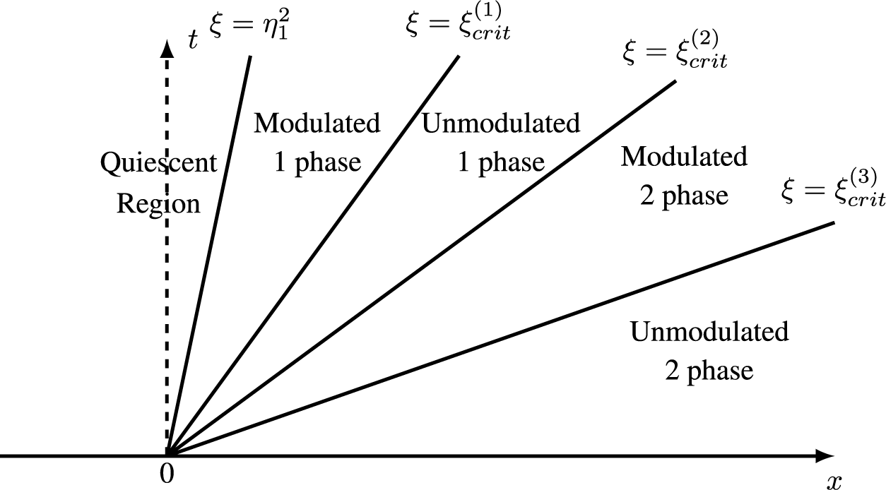


 Open access