


1. Introduction
The canonical problem of a starting object in a quiescent fluid has been investigated for more than a century, where the main focus has been on the force response and the starting vortices. An example is the early work of Prandtl (Reference Prandtl1936), who studied the starting vortex behind a wedge. The motion of an accelerating object in a fluid is relevant to various applications, such as the gust response of surging wings and wind turbine blades (Mancini et al. Reference Mancini, Manar, Granlund, Ol and Jones2015; Eldredge & Jones Reference Eldredge and Jones2019), flapping insect wings (Dickinson, Lehmann & Sane Reference Dickinson, Lehmann and Sane1999; Pullin & Wang Reference Pullin and Wang2004), ship manoeuvring and motion of offshore structures (Lighthill Reference Lighthill1986) and also certain sports, such as the propulsion force generated by a rowing blade (Grift et al. Reference Grift, Vijayaragavan, Tummers and Westerweel2019, Reference Grift, Tummers and Westerweel2021). When an object changes its velocity the kinetic energy of the surrounding fluid must also change. This change in kinetic energy requires work, which is interpreted as the work done by an ‘added mass force’ on the object (Batchelor Reference Batchelor1967; Brennen Reference Brennen1982). In the case of an irrotational flow the added mass force can be computed through potential flow theory and scales linearly with acceleration. This is referred to as the inviscid added mass force. When the surrounding flow contains vorticity, it is often referred to as the circulatory force due to acceleration (e.g. Corkery, Stevens & Babinsky Reference Corkery, Stevens and Babinsky2017), of which the scaling with respect to the motion of the object is not fully known.
Perhaps the most widely used expression for the force on an object that experiences a variation in velocity is the Morison equation (Morison et al. Reference Morison, O’Brien, Johnson and Schaaf1950). This equation separates the time-dependent drag force $F_D(t)$
on an object into a quasisteady drag force
$F_D(t)$
on an object into a quasisteady drag force $F_{\textit{QS}}(t)$
and an acceleration drag force
$F_{\textit{QS}}(t)$
and an acceleration drag force $F_{{a}}(t)$
,
$F_{{a}}(t)$
,
 \begin{equation} F_D(t) = \underbrace {C_{\!D} \textstyle {\dfrac 12}\rho V^2(t) A}_{F_{\textit{QS}}(t)} +F_{{a}}(t), \end{equation}
where $V(t)$
is the instantaneous velocity of the object,
$V(t)$
is the instantaneous velocity of the object, $C_{\!D}$
the steady-state drag coefficient,
$C_{\!D}$
the steady-state drag coefficient, $\rho$
the fluid density and
$\rho$
the fluid density and $A$
the frontal area of the object. The acceleration drag force
$A$
the frontal area of the object. The acceleration drag force $F_{{a}}(t)$
in the original Morison equation is taken equal to the inviscid added mass force
$F_{{a}}(t)$
in the original Morison equation is taken equal to the inviscid added mass force $F_{\textit{AM}} = m_{{h}}a(t)$
, where the (time-dependent) acceleration
$F_{\textit{AM}} = m_{{h}}a(t)$
, where the (time-dependent) acceleration $a(t)$
is multiplied by a constant hydrodynamic mass
$a(t)$
is multiplied by a constant hydrodynamic mass $m_{{h}}$
, which is found from potential flow theory (Batchelor Reference Batchelor1967; Brennen Reference Brennen1982) or determined empirically (Yu Reference Yu1945; Payne Reference Payne1981). When the flow is accelerating and the object is stationary,
$m_{{h}}$
, which is found from potential flow theory (Batchelor Reference Batchelor1967; Brennen Reference Brennen1982) or determined empirically (Yu Reference Yu1945; Payne Reference Payne1981). When the flow is accelerating and the object is stationary, $F_{{a}}(t)$
includes the Froude–Krylov force (Lighthill Reference Lighthill1986). Morison et al. (Reference Morison, O’Brien, Johnson and Schaaf1950) originally considered a variation of fluid velocity due to small-amplitude linear wave motion, which is adequately described by potential flow. This justifies the use of the inviscid added mass force
$F_{{a}}(t)$
includes the Froude–Krylov force (Lighthill Reference Lighthill1986). Morison et al. (Reference Morison, O’Brien, Johnson and Schaaf1950) originally considered a variation of fluid velocity due to small-amplitude linear wave motion, which is adequately described by potential flow. This justifies the use of the inviscid added mass force $F_{\textit{AM}}$
for
$F_{\textit{AM}}$
for $F_{{a}}$
in the original equation. The use of
$F_{{a}}$
in the original equation. The use of $F_{\textit{AM}}$
is also justified for impulsive motions with a (nearly) instantaneous increase in velocity (e.g. von Kármán Reference von Kármán1929), where the flow and its change in kinetic energy are adequately described by potential flow. Using an inviscid added mass force for separated and viscous flows, where the flow pattern changes during the acceleration, is questionable, as noted by both Batchelor (Reference Batchelor1967) and Brennen (Reference Brennen1982).
$F_{\textit{AM}}$
is also justified for impulsive motions with a (nearly) instantaneous increase in velocity (e.g. von Kármán Reference von Kármán1929), where the flow and its change in kinetic energy are adequately described by potential flow. Using an inviscid added mass force for separated and viscous flows, where the flow pattern changes during the acceleration, is questionable, as noted by both Batchelor (Reference Batchelor1967) and Brennen (Reference Brennen1982).
Following Burgers (Reference Burgers1921), an object that is brought into motion in a fluid generates a vortex layer at its surface that diffuses into the fluid due to the viscosity of the fluid, and is subsequently ‘washed away’ by the flow. Then, another vortex layer is formed that also diffuses away, and so on, where the rate per unit of time of impulse to create the subsequent vortex layers forms the drag force experienced by the moving body. The model of Reijtenbagh, Tummers & Westerweel (Reference Reijtenbagh, Tummers and Westerweel2023) is based on this concept, and is used later in this paper to describe the scaling of the force $F_{{a}}(t)$
for accelerating plates. Burgers (Reference Burgers1921) subsequently derives an expression that relates the drag force on an object to the time derivative of the impulse of the fluid motion (see also Biesheuvel & Hagmeijer Reference Biesheuvel and Hagmeijer2006). Wu (Reference Wu1981) and Lighthill (Reference Lighthill1986) arrive independently at the same expression, which is the basis of methods to determine the force on a moving object from the surrounding velocity field (Noca, Shields & Jeon Reference Noca, Shields and Jeon1997; Limacher, Morton & Wood Reference Limacher, Morton and Wood2018; Corkery, Babinsky & Graham Reference Corkery, Babinsky and Graham2019). Several studies have elucidated the role of vortical fluid motion in the resulting forces acting on instationary moving objects; here we focus on recent ones. Pitt Ford & Babinsky (Reference Pitt Ford and Babinsky2013) study the flow around an accelerating plate in a towing tank to determine the inertial effect of the developing leading-edge vortex on the lift force. Fernando, Weymouth & Rival (Reference Fernando, Weymouth and Rival2020) demonstrate that inviscid added mass force does not properly explain the force that acts on a circular plate in a constant-acceleration motion. Later, Reijtenbagh et al. (Reference Reijtenbagh, Tummers and Westerweel2023) find that the peak value of the acceleration drag force
$F_{{a}}(t)$
for accelerating plates. Burgers (Reference Burgers1921) subsequently derives an expression that relates the drag force on an object to the time derivative of the impulse of the fluid motion (see also Biesheuvel & Hagmeijer Reference Biesheuvel and Hagmeijer2006). Wu (Reference Wu1981) and Lighthill (Reference Lighthill1986) arrive independently at the same expression, which is the basis of methods to determine the force on a moving object from the surrounding velocity field (Noca, Shields & Jeon Reference Noca, Shields and Jeon1997; Limacher, Morton & Wood Reference Limacher, Morton and Wood2018; Corkery, Babinsky & Graham Reference Corkery, Babinsky and Graham2019). Several studies have elucidated the role of vortical fluid motion in the resulting forces acting on instationary moving objects; here we focus on recent ones. Pitt Ford & Babinsky (Reference Pitt Ford and Babinsky2013) study the flow around an accelerating plate in a towing tank to determine the inertial effect of the developing leading-edge vortex on the lift force. Fernando, Weymouth & Rival (Reference Fernando, Weymouth and Rival2020) demonstrate that inviscid added mass force does not properly explain the force that acts on a circular plate in a constant-acceleration motion. Later, Reijtenbagh et al. (Reference Reijtenbagh, Tummers and Westerweel2023) find that the peak value of the acceleration drag force $F_{{a}}(t)$
=
$F_{{a}}(t)$
= $F_D(t)\!-\!F_{\textit{QS}}(t)$
does not scale linearly with acceleration, as would be expected for the inviscid added mass force
$F_D(t)\!-\!F_{\textit{QS}}(t)$
does not scale linearly with acceleration, as would be expected for the inviscid added mass force $F_{\textit{AM}}$
, but rather scales with the square root of the acceleration.
$F_{\textit{AM}}$
, but rather scales with the square root of the acceleration.
Alternative approaches to describe the acceleration drag force $F_{{a}}(t)$
in (1.1) have been suggested, such as the vortex force decomposition (Gehlert, Andreu-Angelo & Babinsky Reference Gehlert, Andreu-Angelo and Babinsky2023) that divides the force into circulatory and non-circulatory components, the drift volume approach (McPhaden & Rival Reference McPhaden and Rival2018) and impulse-based methods (Wu Reference Wu1981; Lighthill Reference Lighthill1986; Limacher et al. Reference Limacher, Morton and Wood2018). These methods can be considered data-driven, since they require knowledge of the flow field and flow structures surrounding the object to provide the forces on the moving object. Hence, these methods are not suited to provide an a priori scaling of the drag force with respect to the acceleration of the object. Also, these methods take vorticity to be already present, usually in the form of starting vortices and shear layers, but do not describe explicitly how this vorticity is created. Morton (Reference Morton1984) provides a summary on the generation of vorticity at a wall.
$F_{{a}}(t)$
in (1.1) have been suggested, such as the vortex force decomposition (Gehlert, Andreu-Angelo & Babinsky Reference Gehlert, Andreu-Angelo and Babinsky2023) that divides the force into circulatory and non-circulatory components, the drift volume approach (McPhaden & Rival Reference McPhaden and Rival2018) and impulse-based methods (Wu Reference Wu1981; Lighthill Reference Lighthill1986; Limacher et al. Reference Limacher, Morton and Wood2018). These methods can be considered data-driven, since they require knowledge of the flow field and flow structures surrounding the object to provide the forces on the moving object. Hence, these methods are not suited to provide an a priori scaling of the drag force with respect to the acceleration of the object. Also, these methods take vorticity to be already present, usually in the form of starting vortices and shear layers, but do not describe explicitly how this vorticity is created. Morton (Reference Morton1984) provides a summary on the generation of vorticity at a wall.
Besides experimental studies, there have been numerous numerical studies that focus on the drag force on and the flow field around accelerating and impulsively started plates. Koumoutsakos & Shiels (Reference Koumoutsakos and Shiels1996) use numerical simulations to investigate the vorticity field around a two-dimensional plate in an accelerating flow over a wide range of accelerations with Reynolds numbers between 20 and 1000. They show that the drag coefficients for different accelerations collapse on a single curve, indicating the possible existence of a general scaling law. Pullin & Wang (Reference Pullin and Wang2004) use an inviscid model to describe the flow around an accelerating two-dimensional plate to obtain the unsteady forces that would mimic those of flapping insect wings. Later, Pullin & Sader (Reference Pullin and Sader2021) studied the trailing edge vortex in an inviscid fluid by the start-up motion of a two-dimensional plate, with power laws for both the translational and rotational velocities. Hinton et al. (Reference Hinton, Leonard, Pullin and Sader2024) extended their inviscid theory to an arbitrary two-dimensional body with sharp and straight edges, and formulated similarity solutions for the starting vortex at the trailing edges. Then, Sader et al. (Reference Sader, Hou, Hinton, Pullin and Colonius2024) assessed the inviscid predictions using results from direct numerical simulations. Although related to the present work, their studies mainly focused on the lift force on pitching plates that have an initial small angle of attack, whereas the present work is on the drag force on three-dimensional plates accelerating in a direction normal to the plate surface. Xu & Nitsche (Reference Xu and Nitsche2014) propose scaling laws for impulsively started two-dimensional plates for Reynolds numbers between 250 and 2000, and later determine similar scaling laws for constant and non-constant accelerations (Xu & Nitsche Reference Xu and Nitsche2015). Wang & Eldredge (Reference Wang and Eldredge2013) performed numerical simulations on impulsively started two-dimensional plates at various angles of attack using a viscous vortex particle method for a Reynolds number of 20 000. This low-order method closely resembles the creation and ‘washing away’ of vorticity described by Burgers (Reference Burgers1921).
In this paper we explore the scaling of the acceleration drag force $F_{{a}}(t)$
on plates that accelerate from rest in a stagnant fluid. We consider different types of motion, where a plate undergoes a finite-duration acceleration phase until a certain final velocity is reached, for both constant and non-constant accelerations. This work extends previously reported findings that the original Morison equation, that includes the inviscid added mass, underestimates the actual drag force both during and immediately after the acceleration phase (Reijtenbagh et al. Reference Reijtenbagh, Tummers and Westerweel2023). We measure the drag force on the plate during the entire motion, including a relaxation phase that follows the acceleration phase, where the drag force gradually attains the steady motion drag force, as illustrated in figure 1(a–d) for various examples taken from the full set of measurements over various accelerations
$F_{{a}}(t)$
on plates that accelerate from rest in a stagnant fluid. We consider different types of motion, where a plate undergoes a finite-duration acceleration phase until a certain final velocity is reached, for both constant and non-constant accelerations. This work extends previously reported findings that the original Morison equation, that includes the inviscid added mass, underestimates the actual drag force both during and immediately after the acceleration phase (Reijtenbagh et al. Reference Reijtenbagh, Tummers and Westerweel2023). We measure the drag force on the plate during the entire motion, including a relaxation phase that follows the acceleration phase, where the drag force gradually attains the steady motion drag force, as illustrated in figure 1(a–d) for various examples taken from the full set of measurements over various accelerations $a$
and final velocities
$a$
and final velocities $V_{{a}}$
. These examples illustrate the motivation behind this work. The same data is presented in figure 1(e–h), but now as a function of the dimensionless time
$V_{{a}}$
. These examples illustrate the motivation behind this work. The same data is presented in figure 1(e–h), but now as a function of the dimensionless time $t^*$
, defined as (Gharib, Rambod & Shariff Reference Gharib, Rambod and Shariff1998)
$t^*$
, defined as (Gharib, Rambod & Shariff Reference Gharib, Rambod and Shariff1998)
 \begin{equation} t^* = \frac 1\ell \int _{0}^t V(\tau ) {\rm d}\tau . \end{equation}
This is commonly referred to as the formation time, and it expresses the distance the plate has travelled since the start of the motion ( $t=0$
) in terms of length
$t=0$
) in terms of length $\ell$
. We have chosen the length
$\ell$
. We have chosen the length $\ell$
to be equal to the plate height
$\ell$
to be equal to the plate height $\ell _b$
. The measurements presented in figure 1 are similar to those reported by Grift et al. (Reference Grift, Vijayaragavan, Tummers and Westerweel2019) and Reijtenbagh et al. (Reference Reijtenbagh, Tummers and Westerweel2023); experimental details are given in § 2.
$\ell _b$
. The measurements presented in figure 1 are similar to those reported by Grift et al. (Reference Grift, Vijayaragavan, Tummers and Westerweel2019) and Reijtenbagh et al. (Reference Reijtenbagh, Tummers and Westerweel2023); experimental details are given in § 2.
The measured drag force $F_D(t)$
on a rectangular plate with frontal area
$F_D(t)$
on a rectangular plate with frontal area $A$
=
$A$
= $\ell _a\times \ell _b$
= 0.2
$\ell _a\times \ell _b$
= 0.2 $\times$
0.1 m
$\times$
0.1 m $^2$
for a motion with constant acceleration
$^2$
for a motion with constant acceleration $a$
until it reaches a final velocity
$a$
until it reaches a final velocity $V_{{a}}$
. Different colours represent the results for five repetitions of the same experiment. Data for four different combinations of the acceleration
$V_{{a}}$
. Different colours represent the results for five repetitions of the same experiment. Data for four different combinations of the acceleration $a$
and velocity
$a$
and velocity $V_a$
are plotted as a function of (a–d) time
$V_a$
are plotted as a function of (a–d) time $t$
in seconds, and (e–h) dimensionless time
$t$
in seconds, and (e–h) dimensionless time $t^*$
, defined in (1.2). The black lines indicate the quasisteady drag force,
$t^*$
, defined in (1.2). The black lines indicate the quasisteady drag force, $F_{ {QS}} = C_{\!D}( {1}/{2})\rho V^2(t) A$
(
$F_{ {QS}} = C_{\!D}( {1}/{2})\rho V^2(t) A$
(![]() ); the inviscid added mass force,
); the inviscid added mass force, $F_{\textit{AM}} = m_{{h}}a(t)$
(
$F_{\textit{AM}} = m_{{h}}a(t)$
(![]() ), with
), with $m_{{h}}$
given by Payne (Reference Payne1981); the combined force,
$m_{{h}}$
given by Payne (Reference Payne1981); the combined force, $F_{\textit{QS}}+F_{\textit{AM}}$
(
$F_{\textit{QS}}+F_{\textit{AM}}$
(![]() ). The acceleration phase of the motion is indicated by ‘A’, and the relaxation phase by ‘R’. The shaded area labelled ‘E’ on the left-hand side in each graph indicates the robot engagement at the start of the plate motion, see Appendix A. The roman numerals refer to the flow fields shown in figures 4 and 5.
). The acceleration phase of the motion is indicated by ‘A’, and the relaxation phase by ‘R’. The shaded area labelled ‘E’ on the left-hand side in each graph indicates the robot engagement at the start of the plate motion, see Appendix A. The roman numerals refer to the flow fields shown in figures 4 and 5.

During the acceleration phase of the motion, the drag force $F_D$
increases steadily, until it reaches a peak value at the end of the acceleration phase. When the acceleration ceases, and the plate assumes a constant velocity
$F_D$
increases steadily, until it reaches a peak value at the end of the acceleration phase. When the acceleration ceases, and the plate assumes a constant velocity $V_{{a}}$
, the drag force gradually relaxes to its steady-state value. Five repetitions of the measured drag force are superimposed to illustrate the experimental variation. The black solid lines in figure 1 indicate
$V_{{a}}$
, the drag force gradually relaxes to its steady-state value. Five repetitions of the measured drag force are superimposed to illustrate the experimental variation. The black solid lines in figure 1 indicate $F_{\textit{QS}}+F_{\textit{AM}}$
. The drag force during the acceleration phase of the plate is underestimated, and also, after the acceleration ceases and the plate assumes a constant velocity, the drag force does not suddenly drop to
$F_{\textit{QS}}+F_{\textit{AM}}$
. The drag force during the acceleration phase of the plate is underestimated, and also, after the acceleration ceases and the plate assumes a constant velocity, the drag force does not suddenly drop to $F_{\textit{QS}}$
, as would be predicted by
$F_{\textit{QS}}$
, as would be predicted by $F_{\textit{AM}}$
, but instead gradually relaxes to the steady state value. Evidently, the experimental results in figure 1 for different combinations of acceleration
$F_{\textit{AM}}$
, but instead gradually relaxes to the steady state value. Evidently, the experimental results in figure 1 for different combinations of acceleration $a$
and final velocity
$a$
and final velocity $V_{{a}}$
show that the inviscid added mass force
$V_{{a}}$
show that the inviscid added mass force $F_{\textit{AM}}$
does not properly describe the force during the acceleration and relaxation phases of the motion. The peak in
$F_{\textit{AM}}$
does not properly describe the force during the acceleration and relaxation phases of the motion. The peak in $F_D(t)$
at the initiation of the motion is the result of the engagement of the robot that drives the plate motion, as is explained in Appendix A. Note that when we use
$F_D(t)$
at the initiation of the motion is the result of the engagement of the robot that drives the plate motion, as is explained in Appendix A. Note that when we use $t^*$
for the horizontal axis in figure 1(e–h) the measured drag force
$t^*$
for the horizontal axis in figure 1(e–h) the measured drag force $F_D$
at the start of the motion is compressed towards
$F_D$
at the start of the motion is compressed towards $t^* = 0$
, as the plate barely moves at the start of the motion.
$t^* = 0$
, as the plate barely moves at the start of the motion.
The objective of this experimental study is to expand the approach of Reijtenbagh et al. (Reference Reijtenbagh, Tummers and Westerweel2023) to find a scaling law for the drag force on starting plates. We first consider motions where the acceleration is constant as in the study of Reijtenbagh et al. (Reference Reijtenbagh, Tummers and Westerweel2023). However, in the present work the drag force is considered during the entire motion, rather than only the peak force at the end of the acceleration phase. Also, to test the validity of the model proposed by Reijtenbagh et al. (Reference Reijtenbagh, Tummers and Westerweel2023) motions are repeated in fluids with different viscosities, and we perform measurements for motions with non-constant acceleration. We first consider a motion where the plate is initially at rest and is subsequently accelerated with a constant jerk $J = \dot {a} =$
constant. This motion avoids a discontinuous change in the acceleration at the start of the motion. Finally, we consider a motion where the plate is accelerated such that the velocity increases with the square root of time, i.e.
$J = \dot {a} =$
constant. This motion avoids a discontinuous change in the acceleration at the start of the motion. Finally, we consider a motion where the plate is accelerated such that the velocity increases with the square root of time, i.e. $V(t)\propto \sqrt {t}$
. This motion would predict a constant acceleration drag force
$V(t)\propto \sqrt {t}$
. This motion would predict a constant acceleration drag force $F_{{a}}(t)$
according to the model proposed by Reijtenbagh et al. (Reference Reijtenbagh, Tummers and Westerweel2023).
$F_{{a}}(t)$
according to the model proposed by Reijtenbagh et al. (Reference Reijtenbagh, Tummers and Westerweel2023).
One of the complications of finding proper scaling laws for the drag force during an accelerating motion is that the velocity of the object changes constantly, while the final velocity $V_{{a}}$
at the end of the acceleration phase is yet ‘unknown’ during the acceleration phase. This implies that we cannot identify a proper characteristic velocity of the motion, and thus also cannot identify a proper velocity-based Reynolds number to characterize the fluid motion. Hence, we look for alternative dimensionless numbers that are invariant to the motion. This is further discussed in § 3.
$V_{{a}}$
at the end of the acceleration phase is yet ‘unknown’ during the acceleration phase. This implies that we cannot identify a proper characteristic velocity of the motion, and thus also cannot identify a proper velocity-based Reynolds number to characterize the fluid motion. Hence, we look for alternative dimensionless numbers that are invariant to the motion. This is further discussed in § 3.
An outline of this paper is as follows. Section 2 describes the experimental methods that are used to determine the forces on the accelerating plates, including the experimental facility, the different motions, the geometries of the plates and the different working fluids, in addition to the methods used to measure the forces and flow field. Section 3 explains the model that describes the acceleration drag force $F_{{a}}(t)$
during the acceleration phase and subsequent relaxation phase. Also a modified Reynolds number is identified that does not explicitly depend on the velocity. This acceleration Reynolds number is used to scale the acceleration drag force. Sections 4 and 5 present the results of the experiments for both the constant acceleration and non-constant acceleration motions. The main conclusions of this study are summarized in § 6.
$F_{{a}}(t)$
during the acceleration phase and subsequent relaxation phase. Also a modified Reynolds number is identified that does not explicitly depend on the velocity. This acceleration Reynolds number is used to scale the acceleration drag force. Sections 4 and 5 present the results of the experiments for both the constant acceleration and non-constant acceleration motions. The main conclusions of this study are summarized in § 6.
2. Experiments
2.1. Experimental set-up
Figure 2 shows the experimental set-up, which is identical to that of Grift et al. (Reference Grift, Vijayaragavan, Tummers and Westerweel2019). It consists of a rectangular plate with an aspect ratio of 1 : 2 (AR = 2) with a width $\ell _a$
of 0.200 m, a height
$\ell _a$
of 0.200 m, a height $\ell _b$
of 0.100 m and thickness
$\ell _b$
of 0.100 m and thickness $\ell _c$
of 4 mm, connected to an industrial gantry robot (Reis Robotics RL50). The plate is translated through a 2.00
$\ell _c$
of 4 mm, connected to an industrial gantry robot (Reis Robotics RL50). The plate is translated through a 2.00 $\times$
2.00
$\times$
2.00 $\times$
0.60 m
$\times$
0.60 m $^3$
water-filled tank, with a water height of 0.50 m. The top of this plate is 1.5
$^3$
water-filled tank, with a water height of 0.50 m. The top of this plate is 1.5 $\ell _b$
below the water surface, so that it can be considered fully submerged (Grift et al. Reference Grift, Vijayaragavan, Tummers and Westerweel2019). With a frontal area of
$\ell _b$
below the water surface, so that it can be considered fully submerged (Grift et al. Reference Grift, Vijayaragavan, Tummers and Westerweel2019). With a frontal area of $A$
=
$A$
= $\ell _a\times \ell _b$
= 0.020 m
$\ell _a\times \ell _b$
= 0.020 m $^2$
, the blockage ratio is 0.02, which is well below the value of 0.06 for which walls may begin to influence the drag force (West & Apelt Reference West and Apelt1982). In addition to this rectangular plate, a square plate and a circular plate, both with
$^2$
, the blockage ratio is 0.02, which is well below the value of 0.06 for which walls may begin to influence the drag force (West & Apelt Reference West and Apelt1982). In addition to this rectangular plate, a square plate and a circular plate, both with $A$
= 200.0 cm
$A$
= 200.0 cm $^2$
, are also tested, in addition to AR = 2 rectangular plates with frontal areas of 312.5 and 112.5 cm
$^2$
, are also tested, in addition to AR = 2 rectangular plates with frontal areas of 312.5 and 112.5 cm $^2$
, respectively, see § 4.2. All plates are made of acrylic and have the same thickness, i.e. 4 mm.
$^2$
, respectively, see § 4.2. All plates are made of acrylic and have the same thickness, i.e. 4 mm.
Schematic of the experimental set-up, viewed from the side (a) and from above (b), consisting of a large water-filled tank, with a gantry robot moving a plate with a prescribed motion. A light sheet illuminates a planar cross-section of the flow through the middle of the plate. A digital high-speed camera is positioned below the water-filled tank and observes the flow through a $45^\circ$
mirror. The shaded area represents the field-of-view of the camera. For the measurements in the water–glycerol mixtures at elevated viscosities a smaller tank, outlined by the dotted line, is placed inside the larger tank, see text for further details. Photographs of the experimental set-up are available as Supplementary material at https://doi.org/10.1017/jfm.2025.11107.
$45^\circ$
mirror. The shaded area represents the field-of-view of the camera. For the measurements in the water–glycerol mixtures at elevated viscosities a smaller tank, outlined by the dotted line, is placed inside the larger tank, see text for further details. Photographs of the experimental set-up are available as Supplementary material at https://doi.org/10.1017/jfm.2025.11107.

The use of thin plates, instead of streamlined bodies, has the advantage that the quasisteady drag coefficient $C_{\!D}$
in (1.1) hardly varies with the Reynolds number
$C_{\!D}$
in (1.1) hardly varies with the Reynolds number ${\textit{Re}}$
when
${\textit{Re}}$
when ${\textit{Re}}$ $\gt 10^3$
(Blevins Reference Blevins2003), see also § 3.1.
$\gt 10^3$
(Blevins Reference Blevins2003), see also § 3.1.
In this paper we focus on measurements of the drag force on AR = 2 rectangular plates, following Ringuette, Milano & Gharib (Reference Ringuette, Milano and Gharib2007), Grift et al. (Reference Grift, Vijayaragavan, Tummers and Westerweel2019) and Reijtenbagh et al. (Reference Reijtenbagh, Tummers and Westerweel2023). One can argue that it makes more sense to primarily consider a circular plate, and later test for other geometries. There are two main reasons for using the rectangular AR = 2 plate. As shown by Fernando & Rival (Reference Fernando and Rival2016) and Grift et al. (Reference Grift, Vijayaragavan, Tummers and Westerweel2019), there are clear peaks in the drag force at certain values of $t^*$
that occur due to significant changes in the originally formed vortex ring behind a circular plate. Also, Fernando & Rival (Reference Fernando and Rival2016) and Fernando et al. (Reference Fernando, Weymouth and Rival2020) show that circular plates show a large decrease of
$t^*$
that occur due to significant changes in the originally formed vortex ring behind a circular plate. Also, Fernando & Rival (Reference Fernando and Rival2016) and Fernando et al. (Reference Fernando, Weymouth and Rival2020) show that circular plates show a large decrease of $F_D$
after the acceleration phase until
$F_D$
after the acceleration phase until $t^* \approx 20$
, even below what is expected from a steady-state drag force. With this in mind, one could question the validity of (1.1) during the relaxation phase of the motion, and even during the acceleration phase. These complications do not appear to occur for rectangular plates, where the drag force
$t^* \approx 20$
, even below what is expected from a steady-state drag force. With this in mind, one could question the validity of (1.1) during the relaxation phase of the motion, and even during the acceleration phase. These complications do not appear to occur for rectangular plates, where the drag force $F_D$
during the relaxation phase decays more or less gradually to the expected steady-state value, see figure 1.
$F_D$
during the relaxation phase decays more or less gradually to the expected steady-state value, see figure 1.
The robot is programmed to move the plates through the fluid along a straight path in the middle of the tank. The start and end positions of the plate are at least three times the plate height from the front and rear facing tank walls. Previously Grift et al. (Reference Grift, Vijayaragavan, Tummers and Westerweel2019) showed that the flow remains unperturbed over a distance 2.4 times the plate height in front of the plate.
Additional measurements are performed in a smaller tank (with dimensions of 1.50 $\times$
0.75
$\times$
0.75 $\times$
0.60 m
$\times$
0.60 m $^3$
) for three different water–glycerol mixtures to investigate the effect of the fluid viscosity
$^3$
) for three different water–glycerol mixtures to investigate the effect of the fluid viscosity $\nu$
, see table 1. The smaller tank is designed such that the plates can reach a final velocity
$\nu$
, see table 1. The smaller tank is designed such that the plates can reach a final velocity $V_{{a}}$
of 0.90 m s−1 for a large range of accelerations without any wall effects by keeping the blockage ratio of the rectangular plate below 0.06. The finite length of the smaller tank limits the final plate velocity
$V_{{a}}$
of 0.90 m s−1 for a large range of accelerations without any wall effects by keeping the blockage ratio of the rectangular plate below 0.06. The finite length of the smaller tank limits the final plate velocity $V_{{a}}$
to 0.90 m s−1. The full range of experiments with constant accelerations is given by table 2. The motions in experiments with non-constant accelerations are shown in figure 3 and details of these experiments are given in table 3.
$V_{{a}}$
to 0.90 m s−1. The full range of experiments with constant accelerations is given by table 2. The motions in experiments with non-constant accelerations are shown in figure 3 and details of these experiments are given in table 3.
The dynamic viscosity $\mu$
, density
$\mu$
, density $\rho$
and kinematic viscosity
$\rho$
and kinematic viscosity $\nu$
of water (V1) and water–glycerol mixtures (V2–4).
$\nu$
of water (V1) and water–glycerol mixtures (V2–4).

Overview of the accelerations $a$
and final velocities
$a$
and final velocities $V_{{a}}$
in the constant-acceleration experiments with the AR = 2 rectangular plate. Crosses indicate the combinations of acceleration and velocity that are done with water only; dots indicate the combinations of acceleration and velocity with water and water–glycerol mixtures at higher viscosities. The Reynolds number
$V_{{a}}$
in the constant-acceleration experiments with the AR = 2 rectangular plate. Crosses indicate the combinations of acceleration and velocity that are done with water only; dots indicate the combinations of acceleration and velocity with water and water–glycerol mixtures at higher viscosities. The Reynolds number ${\textit{Re}}$
is given by the velocity
${\textit{Re}}$
is given by the velocity $V_{{a}}$
, the plate height
$V_{{a}}$
, the plate height $\ell _b$
and the kinematic viscosity
$\ell _b$
and the kinematic viscosity $\nu$
of the fluid, i.e. either water (V1) or the water–glycerol mixtures (V2–V4), see table 1.
$\nu$
of the fluid, i.e. either water (V1) or the water–glycerol mixtures (V2–V4), see table 1.

The plate is connected to the gantry robot with a streamlined strut. We use either of two force sensors between the robot and the plate, where one sensor (ATI Gamma 32-2.5) is used for measurements with lower final velocities ( $V_{{a}}\lt$
0.6 m s−1), while the other sensor (ATI Delta 660-60) is used for those with higher velocities (
$V_{{a}}\lt$
0.6 m s−1), while the other sensor (ATI Delta 660-60) is used for those with higher velocities ( $V_{{a}}\geqslant$
0.6 m s−1). The force signals are filtered using a low-pass filter with a 15 Hz cutoff frequency to reduce noise in the measured signal that originates from the robot (Grift et al. Reference Grift, Vijayaragavan, Tummers and Westerweel2019). The drag force
$V_{{a}}\geqslant$
0.6 m s−1). The force signals are filtered using a low-pass filter with a 15 Hz cutoff frequency to reduce noise in the measured signal that originates from the robot (Grift et al. Reference Grift, Vijayaragavan, Tummers and Westerweel2019). The drag force $F_D(t)$
is found from the measured force
$F_D(t)$
is found from the measured force $F(t)$
by subtracting the inertia
$F(t)$
by subtracting the inertia $m_pa(t)$
of the plate and the strut, where
$m_pa(t)$
of the plate and the strut, where $m_p$
is their combined mass, and the (very small) measured drag imposed by the strut.
$m_p$
is their combined mass, and the (very small) measured drag imposed by the strut.
Examples of the programmed plate motions with prescribed (a) velocity $V(t)$
, (b) acceleration
$V(t)$
, (b) acceleration $a(t)$
and (c) jerk
$a(t)$
and (c) jerk $J(t)$
: constant acceleration (blue); quadratic velocity motion (green); square-root velocity motion (red). Dashed lines indicate discontinuities in acceleration or jerk. In this example, the final velocity is
$J(t)$
: constant acceleration (blue); quadratic velocity motion (green); square-root velocity motion (red). Dashed lines indicate discontinuities in acceleration or jerk. In this example, the final velocity is $V_{{a}}$
= 0.6 m s−1, see tables 2 and 3 for an overview of all motions.
$V_{{a}}$
= 0.6 m s−1, see tables 2 and 3 for an overview of all motions.

2.2. Particle image velocimetry
Planar particle image velocimetry (PIV) is used to characterize the flow around the plates. A high-speed camera (Phantom VEO 640 L) is used to record 2560 $\times$
1600 pixel images at a rate of 1000 frames per second of small neutrally buoyant fluorescent tracer particles (Cospheric UVPMS-BR-0.995, with 53–63
$\times$
1600 pixel images at a rate of 1000 frames per second of small neutrally buoyant fluorescent tracer particles (Cospheric UVPMS-BR-0.995, with 53–63 $\unicode{x03BC}$
m diameter) suspended in the water-filled tank. A 4 mm-thick light sheet from a frequency-doubled Nd:YLF pulsed laser (Litron LDY304-PIV, 527 nm light wavelength) illuminates the tracer particles in a planar cross-section of the tank. The camera and laser sheet are set up to ensure that the field of view is through the centre of the plate in a horizontal plane. This two-dimensional field is representative of the three-dimensional flow around the plate. The field of view has dimensions of 913
$\unicode{x03BC}$
m diameter) suspended in the water-filled tank. A 4 mm-thick light sheet from a frequency-doubled Nd:YLF pulsed laser (Litron LDY304-PIV, 527 nm light wavelength) illuminates the tracer particles in a planar cross-section of the tank. The camera and laser sheet are set up to ensure that the field of view is through the centre of the plate in a horizontal plane. This two-dimensional field is representative of the three-dimensional flow around the plate. The field of view has dimensions of 913 $\times$
477 mm
$\times$
477 mm $^2$
, which is sufficient to capture the full width of the wake and to follow the plate over a distance of more than six times the plate height (i.e.
$^2$
, which is sufficient to capture the full width of the wake and to follow the plate over a distance of more than six times the plate height (i.e. $t^* \gt 6)$
.
$t^* \gt 6)$
.
Overview of three accelerating motions with velocity $V \propto t^n$
and acceleration
$V \propto t^n$
and acceleration $a \propto t^{n-1}$
, with
$a \propto t^{n-1}$
, with $n$
= 1, 2 and
$n$
= 1, 2 and $\textstyle 1/2$
; these correspond to ‘zero jerk’ (
$\textstyle 1/2$
; these correspond to ‘zero jerk’ ( $J=0$
), ‘positive jerk’ (
$J=0$
), ‘positive jerk’ ( $J\gt 0$
) and ‘negative jerk’ (
$J\gt 0$
) and ‘negative jerk’ ( $J\lt 0$
) motions, respectively. The scaling for the force
$J\lt 0$
) motions, respectively. The scaling for the force $F_{{a}}$
is according to the model in (3.1) proposed by Reijtenbagh et al. (Reference Reijtenbagh, Tummers and Westerweel2023).
$F_{{a}}$
is according to the model in (3.1) proposed by Reijtenbagh et al. (Reference Reijtenbagh, Tummers and Westerweel2023).

The PIV images are analysed using commercial software (Davis 10.2, LaVision GmbH), using a multipass sliding sum-of-correlation method between the $n$
th frame and (
$n$
th frame and ( $n$
+ 2)th frame, with 48
$n$
+ 2)th frame, with 48 $\times$
48-pixel interrogation regions at the initial pass to 24
$\times$
48-pixel interrogation regions at the initial pass to 24 $\times$
24-pixel windows at the final pass, and with 50 % overlap between adjacent interrogations windows. The final result for the velocity fields has a data spacing of 4.19 mm (i.e. 8.37 mm spatial resolution). The velocities in the final results pass a universal outlier detection test (Westerweel & Scarano Reference Westerweel and Scarano2005), indicating that the results contain at least 99.8 % valid data; rejected interrogation results are replaced by linear interpolation.
$\times$
24-pixel windows at the final pass, and with 50 % overlap between adjacent interrogations windows. The final result for the velocity fields has a data spacing of 4.19 mm (i.e. 8.37 mm spatial resolution). The velocities in the final results pass a universal outlier detection test (Westerweel & Scarano Reference Westerweel and Scarano2005), indicating that the results contain at least 99.8 % valid data; rejected interrogation results are replaced by linear interpolation.
3. Model
3.1. Background
Our point of departure is Morison’s equation (1.1) as modified by Reijtenbagh et al. (Reference Reijtenbagh, Tummers and Westerweel2023) to describe the drag force on an accelerating plate. The quasisteady force remains unchanged, and instead of the conventional inviscid added mass for the acceleration drag force $F_{{a}}(t)$
we use a history-based acceleration drag force. Reijtenbagh et al. (Reference Reijtenbagh, Tummers and Westerweel2023) showed that this gives a better representation of the total drag force. Figure 4 shows the flow field around the plate at different dimensionless times. Figure 4(a) shows the potential flow solution for a moving plate, which resembles the measured flow field at
$F_{{a}}(t)$
we use a history-based acceleration drag force. Reijtenbagh et al. (Reference Reijtenbagh, Tummers and Westerweel2023) showed that this gives a better representation of the total drag force. Figure 4 shows the flow field around the plate at different dimensionless times. Figure 4(a) shows the potential flow solution for a moving plate, which resembles the measured flow field at $t^*=0.05$
in figure 4(b). This indicates that at these short times potential flow, and therefore inviscid added mass, remains a good approximation of the flow and drag force on the plate, although evidence of vorticity at the plate edges is visible. However, note that here
$t^*=0.05$
in figure 4(b). This indicates that at these short times potential flow, and therefore inviscid added mass, remains a good approximation of the flow and drag force on the plate, although evidence of vorticity at the plate edges is visible. However, note that here $t^*$
= 0.05 corresponds to a plate displacement of 5 mm that is just slightly larger than the plate thickness (4 mm).
$t^*$
= 0.05 corresponds to a plate displacement of 5 mm that is just slightly larger than the plate thickness (4 mm).
The flow around an accelerating AR = 2 rectangular plate. (a) Potential flow around a flat plate, with streamlines in blue. The measured flow around the plate for $a$
= 0.82 m s−2 and
$a$
= 0.82 m s−2 and $V_{{a}}$
= 0.40 m s−1 (corresponding to
$V_{{a}}$
= 0.40 m s−1 (corresponding to ${\textit{Re}}$
= 40
${\textit{Re}}$
= 40 $\times$
10
$\times$
10 $^3$
) at dimensionless times:
$^3$
) at dimensionless times: $t^*$
= 0.05 (b), 0.10 (c), 0.20 (d) and 0.75 (e), respectively, in a fixed frame of reference. The panels (b–e) correspond to the roman numerals I–IV in figure 1. Panels (f–i) represent the same data as (b–e), but now represented in a frame of reference moving with the plate. The colour scale indicates dimensionless out-of-plane component of the vorticity
$t^*$
= 0.05 (b), 0.10 (c), 0.20 (d) and 0.75 (e), respectively, in a fixed frame of reference. The panels (b–e) correspond to the roman numerals I–IV in figure 1. Panels (f–i) represent the same data as (b–e), but now represented in a frame of reference moving with the plate. The colour scale indicates dimensionless out-of-plane component of the vorticity $\omega ^* = \omega _z \ell _b / V_{{a}}$
. Dimensions (
$\omega ^* = \omega _z \ell _b / V_{{a}}$
. Dimensions ( $x$
,
$x$
, $y$
) are made dimensionless with the plate height
$y$
) are made dimensionless with the plate height $\ell _b$
. For clarity only one out of four velocity vectors is shown.
$\ell _b$
. For clarity only one out of four velocity vectors is shown.

When the plate further progresses during the acceleration the flow starts to separate and a starting vortex loop is created (Grift et al. Reference Grift, Vijayaragavan, Tummers and Westerweel2019), visible as the vortex pair in figure 4(c). Here, potential flow is no longer appropriate to describe the flow, and therefore is not a proper basis for estimating the acceleration drag force $F_{{a}}(t)$
. This is in line with earlier derivations (Burgers Reference Burgers1921; Biesheuvel & Hagmeijer Reference Biesheuvel and Hagmeijer2006; Limacher et al. Reference Limacher, Morton and Wood2018) where the acceleration drag force is equal to inviscid added mass at early stages only, without flow separation, and where the vorticity is only present in a thin boundary layer close to the plate. This boundary layer is readily visible in figure 4(d–e) (see also figure 18 in Appendix B) and figure 4(h–i), where the flow field is represented in a frame of reference that moves with the plate. The incoming flow impinging on the plate resembles a Hiemenz flow (Emanuel Reference Emanuel2000), which is that of a stationary irrotational outer flow that resembles a stagnation point flow with a viscous boundary layer with a thickness that is inversely proportional to the square root of the flow Reynolds number. The moving plate in the fluid generates vorticity at the surface that diffuses into the fluid and then advects to the edges of the plate where it accumulates in the vortex (Burgers Reference Burgers1921; Biesheuvel & Hagmeijer Reference Biesheuvel and Hagmeijer2006). Figure 5 shows the further development of the instantaneous flow to illustrate the transition of the flow into that of a turbulent wake.
$F_{{a}}(t)$
. This is in line with earlier derivations (Burgers Reference Burgers1921; Biesheuvel & Hagmeijer Reference Biesheuvel and Hagmeijer2006; Limacher et al. Reference Limacher, Morton and Wood2018) where the acceleration drag force is equal to inviscid added mass at early stages only, without flow separation, and where the vorticity is only present in a thin boundary layer close to the plate. This boundary layer is readily visible in figure 4(d–e) (see also figure 18 in Appendix B) and figure 4(h–i), where the flow field is represented in a frame of reference that moves with the plate. The incoming flow impinging on the plate resembles a Hiemenz flow (Emanuel Reference Emanuel2000), which is that of a stationary irrotational outer flow that resembles a stagnation point flow with a viscous boundary layer with a thickness that is inversely proportional to the square root of the flow Reynolds number. The moving plate in the fluid generates vorticity at the surface that diffuses into the fluid and then advects to the edges of the plate where it accumulates in the vortex (Burgers Reference Burgers1921; Biesheuvel & Hagmeijer Reference Biesheuvel and Hagmeijer2006). Figure 5 shows the further development of the instantaneous flow to illustrate the transition of the flow into that of a turbulent wake.
Reijtenbagh et al. (Reference Reijtenbagh, Tummers and Westerweel2023) use Stokes’ first problem as an ansatz for a model that incorporates the generation and diffusion of vorticity for an accelerating plate. This is then generalized to account for the advection of vorticity along the plate surface, which leads to a model where the acceleration drag force $F_{{a}}(t)$
is proportional to
$F_{{a}}(t)$
is proportional to $\sqrt {aV}$
. The derivation of this model is summarized in Appendix B.
$\sqrt {aV}$
. The derivation of this model is summarized in Appendix B.
The instantaneous flow field around an accelerating AR = 2 rectangular plate in the same experiment as in figure 4, at dimensionless times $t^*$
= 2.0 (a), 3.0 (b), 4.0 (c), 5.0 (d) and 7.0 (e), respectively. Dimensions (
$t^*$
= 2.0 (a), 3.0 (b), 4.0 (c), 5.0 (d) and 7.0 (e), respectively. Dimensions ( $x$
,
$x$
, $y$
) are made dimensionless with the plate height
$y$
) are made dimensionless with the plate height $\ell _b$
. For clarity only one out of four velocity vectors is shown. The colours represent the dimensionless out-of-plane component of the vorticity
$\ell _b$
. For clarity only one out of four velocity vectors is shown. The colours represent the dimensionless out-of-plane component of the vorticity $\omega ^* = \omega _z\ell _b/V_{{a}}$
. The roman numerals correspond to those in figure 1.
$\omega ^* = \omega _z\ell _b/V_{{a}}$
. The roman numerals correspond to those in figure 1.

3.2. Acceleration drag force
Combining the results of Xu & Nitsche (Reference Xu and Nitsche2015) and Reijtenbagh et al. (Reference Reijtenbagh, Tummers and Westerweel2023) we find for the acceleration drag force $F_{{a}}(t)$
,
$F_{{a}}(t)$
,
 \begin{equation} F_{{a}}(t) = \underbrace {C\frac {a^{1/4}\ell ^{3/4}}{\nu ^{1/2}}}_{C_{{a}}}\rho A \sqrt {\nu a V}, \end{equation}
where $C$
is an empirical constant and
$C$
is an empirical constant and $\ell$
an appropriate length scale. Note that
$\ell$
an appropriate length scale. Note that $\sqrt {aV} = at^{1/2}$
for a constant acceleration
$\sqrt {aV} = at^{1/2}$
for a constant acceleration $a$
. Rewriting (3.1) by eliminating
$a$
. Rewriting (3.1) by eliminating $\sqrt \nu$
gives
$\sqrt \nu$
gives
 \begin{equation} F_{{a}}(t) \cong m_{{h}}(t) a, \quad \text{with}\quad m_{{h}}(t) = \rho A \ell _{{h}}(t), \end{equation}
where $\ell _{{h}}(t)$
(
$\ell _{{h}}(t)$
( $=Ca^{1/4}\ell ^{3/4}t^{1/2}$
) absorbs the time dependency of (3.1) and other remaining constants, and
$=Ca^{1/4}\ell ^{3/4}t^{1/2}$
) absorbs the time dependency of (3.1) and other remaining constants, and $m_{{h}}(t)$
represents a time-dependent ‘hydrodynamic mass’ of the accelerating plate (Grift et al. Reference Grift, Vijayaragavan, Tummers and Westerweel2019). The length scale
$m_{{h}}(t)$
represents a time-dependent ‘hydrodynamic mass’ of the accelerating plate (Grift et al. Reference Grift, Vijayaragavan, Tummers and Westerweel2019). The length scale $\ell _{{h}}(t)$
would represent the dimension of the ‘volume of fluid’
$\ell _{{h}}(t)$
would represent the dimension of the ‘volume of fluid’ $A\ell _{{h}}(t)$
that is thought to be accelerated along with the moving plate (Batchelor Reference Batchelor1967). Evidently, the acceleration drag force is not constant, as opposed to the conventional inviscid added mass force obtained from potential flow, which implies
$A\ell _{{h}}(t)$
that is thought to be accelerated along with the moving plate (Batchelor Reference Batchelor1967). Evidently, the acceleration drag force is not constant, as opposed to the conventional inviscid added mass force obtained from potential flow, which implies $m_{{h}}(t)$
grows during acceleration, and (3.2) would represent a generalized approach where the flow can also be rotational. However, the concept of hydrodynamic mass in (3.2) would also imply that
$m_{{h}}(t)$
grows during acceleration, and (3.2) would represent a generalized approach where the flow can also be rotational. However, the concept of hydrodynamic mass in (3.2) would also imply that $F_{{a}}(t)$
vanishes when
$F_{{a}}(t)$
vanishes when $a=0$
, which is evidently not the case, see figure 1. Therefore, the association of
$a=0$
, which is evidently not the case, see figure 1. Therefore, the association of $F_{{a}}(t)$
with a ‘hydrodynamic mass’ does not seem appropriate in this context.
$F_{{a}}(t)$
with a ‘hydrodynamic mass’ does not seem appropriate in this context.
The dimensionless prefactor $C_ {{a}}$
in (3.1) is rewritten as
$C_ {{a}}$
in (3.1) is rewritten as
 \begin{equation} C_{{a}} = C\frac {a^{1/4}\ell ^{3/4}}{\nu ^{1/2}} = C\left (\frac {a\ell }{V^2}\right )^{1/4} \frac {V^{1/2}\ell ^{1/2}}{\nu ^{1/2}} = C\left (a^*\right )^{1/4}{\textit{Re}}^{1/2}, \end{equation}
where $a^* = a\ell /V^2$
is the dimensionless acceleration defined with respect to the velocity
$a^* = a\ell /V^2$
is the dimensionless acceleration defined with respect to the velocity $V$
of the moving plate, and
$V$
of the moving plate, and ${\textit{Re}}$
the Reynolds number defined by the velocity
${\textit{Re}}$
the Reynolds number defined by the velocity $V$
, the plate dimension
$V$
, the plate dimension $\ell$
and the kinematic viscosity
$\ell$
and the kinematic viscosity $\nu$
. The constant
$\nu$
. The constant $C$
is determined experimentally, see § 4.1. It depends on the plate geometry, i.e. AR = 2 rectangular, square or circular plate, but also on the motion; it absorbs the constants
$C$
is determined experimentally, see § 4.1. It depends on the plate geometry, i.e. AR = 2 rectangular, square or circular plate, but also on the motion; it absorbs the constants $C_n$
, with
$C_n$
, with $n$
= 1, 2 and 1/2, that arise from the history-based model explained in Appendix B.
$n$
= 1, 2 and 1/2, that arise from the history-based model explained in Appendix B.
Hence, the acceleration drag force $F_{{a}}(t)$
for constant acceleration motion (
$F_{{a}}(t)$
for constant acceleration motion ( $n=1$
),
$n=1$
), $V(t)=at$
; constant jerk motion (
$V(t)=at$
; constant jerk motion ( $n=2$
),
$n=2$
), $V(t) = \textstyle (1/2) Jt^2$
; ‘square-root velocity’ motion (
$V(t) = \textstyle (1/2) Jt^2$
; ‘square-root velocity’ motion ( $n=1/2$
),
$n=1/2$
), $V(t)=Q\sqrt {t}$
, given by the history-based model become
$V(t)=Q\sqrt {t}$
, given by the history-based model become
 \begin{equation} F_{{a}}(t) = C_{{a}}\rho A \sqrt \nu \begin{cases} at^{1/2} & n=1,\\ Jt^{3/2} &n=2,\\ Qt^0 &n=\textstyle \dfrac 12. \end{cases} \end{equation}
When the motions are expressed in terms of $t^*$
, defined in (1.2), we find
$t^*$
, defined in (1.2), we find

Note that for the square-root velocity motion ( $n$
= 1/2),
$n$
= 1/2), $t^*$
=
$t^*$
= $\textstyle ( 2/3)(Q/\ell _b)t^{3/2}$
.
$\textstyle ( 2/3)(Q/\ell _b)t^{3/2}$
.
3.3. Acceleration Reynolds number
The expression in (3.3) can be written as
 \begin{equation} C_{{a}} = C\sqrt {{\textit{Re}}_{{a}}}, \end{equation}
where ${\textit{Re}}_{{a}}$
is given by
${\textit{Re}}_{{a}}$
is given by
 \begin{equation} {\textit{Re}}_{{a}} = \sqrt {a^*} Re. \end{equation}
This definition of an acceleration Reynolds number ${\textit{Re}}_{{a}}$
is convenient since it eliminates the velocity
${\textit{Re}}_{{a}}$
is convenient since it eliminates the velocity $V$
, so what is left is a Reynolds number
$V$
, so what is left is a Reynolds number ${\textit{Re}}_{{a}}$
that only depends on acceleration. This Reynolds number is equivalent to the acceleration-based Reynolds number introduced by Freymuth, Bank & Palmer (Reference Freymuth, Bank and Palmer1983) and generalized by Xu & Nitsche (Reference Xu and Nitsche2015) and is equal to the square root of the dimensionless acceleration
${\textit{Re}}_{{a}}$
that only depends on acceleration. This Reynolds number is equivalent to the acceleration-based Reynolds number introduced by Freymuth, Bank & Palmer (Reference Freymuth, Bank and Palmer1983) and generalized by Xu & Nitsche (Reference Xu and Nitsche2015) and is equal to the square root of the dimensionless acceleration $\alpha = a \ell ^3 / \nu ^2$
defined by Koumoutsakos & Shiels (Reference Koumoutsakos and Shiels1996).
$\alpha = a \ell ^3 / \nu ^2$
defined by Koumoutsakos & Shiels (Reference Koumoutsakos and Shiels1996).
The dimensionless acceleration $a^* = a\ell /V^2$
requires further clarification, especially for the non-constant accelerations of the plate. Our point of departure is the Morison equation, which has two terms: one is the quasisteady drag force
$a^* = a\ell /V^2$
requires further clarification, especially for the non-constant accelerations of the plate. Our point of departure is the Morison equation, which has two terms: one is the quasisteady drag force $F_{\textit{QS}}$
and the other one is the acceleration drag force
$F_{\textit{QS}}$
and the other one is the acceleration drag force $F_{{a}}$
that is due to the acceleration of the surrounding fluid. In the original expression
$F_{{a}}$
that is due to the acceleration of the surrounding fluid. In the original expression $F_{{a}}$
is taken equal to the inviscid added mass force
$F_{{a}}$
is taken equal to the inviscid added mass force $F_{\textit{AM}}$
that is associated with potential flow. For a fully submerged AR = 2 rectangular plate, with
$F_{\textit{AM}}$
that is associated with potential flow. For a fully submerged AR = 2 rectangular plate, with $A$
=
$A$
= $\ell _a\times \ell _b$
, the drag coefficient is
$\ell _a\times \ell _b$
, the drag coefficient is $C_{\!D}$
= 1.3 (Grift et al. Reference Grift, Vijayaragavan, Tummers and Westerweel2019). For thin plates the drag coefficient
$C_{\!D}$
= 1.3 (Grift et al. Reference Grift, Vijayaragavan, Tummers and Westerweel2019). For thin plates the drag coefficient $C_{\!D}$
is effectively constant over a large range of Reynolds numbers
$C_{\!D}$
is effectively constant over a large range of Reynolds numbers ${\textit{Re}} \gg 10^3$
(Hoerner Reference Hoerner1965; Blevins Reference Blevins2003). The inviscid added mass force
${\textit{Re}} \gg 10^3$
(Hoerner Reference Hoerner1965; Blevins Reference Blevins2003). The inviscid added mass force $F_{\textit{AM}}$
for a rectangular plate is (Brennen Reference Brennen1982)
$F_{\textit{AM}}$
for a rectangular plate is (Brennen Reference Brennen1982)
 \begin{equation} F_{\textit{AM}} = 0.84\frac \pi 4\rho \ell _a\ell _b^2a. \end{equation}
The ratio of the added mass force and the quasisteady drag force, with $C_{\!D}=1.3$
, is then
$C_{\!D}=1.3$
, is then
 \begin{equation} \frac {F_{\textit{AM}}}{F_{\textit{QS}}} = \frac {0.84\dfrac \pi 4\rho \ell _a\ell _b^2a}{1.3\times \textstyle \dfrac 12\rho V^2\ell _a\ell _b} = \underbrace {\frac {0.84\dfrac \pi 4}{1.3\times \textstyle \frac 12}}_{1.01}\frac {a\ell _b}{V^2} \cong a^*, \end{equation}
where $\ell _b$
is the short dimension of the plate, here referred to as the plate height; the numerical prefactor is close to unity, and therefore ignored here. Hence, the dimensionless acceleration
$\ell _b$
is the short dimension of the plate, here referred to as the plate height; the numerical prefactor is close to unity, and therefore ignored here. Hence, the dimensionless acceleration $a^*$
can be interpreted as the ratio of the added mass force relative to the quasisteady drag force.
$a^*$
can be interpreted as the ratio of the added mass force relative to the quasisteady drag force.
We can take the same approach for the cases with non-constant accelerations, where both $a_n$
and
$a_n$
and $V_n$
vary in time (see table 3), such that for
$V_n$
vary in time (see table 3), such that for $n=2$
$n=2$
 \begin{equation} a_2 = Jt \quad \text{and}\quad V_2(t) = \frac {1}{2}Jt^2, \end{equation}
where $J$
is the jerk in
$J$
is the jerk in $\rm [m\,s^{-3}]$
and
$\rm [m\,s^{-3}]$
and $n=1/2$
gives
$n=1/2$
gives
 \begin{equation} a_{1/2}(t) = \frac {1}{2}Qt^{-1/2}, \quad \text{and}\quad V_{1/2}(t) = Qt^{1/2}. \end{equation}
Substituting (3.10) and (3.11) in the definition for $a^*$
gives
$a^*$
gives
 \begin{equation} a^*_2 = \frac {a_2\ell _b}{V_2^2}=\frac {Jt\ell _b}{\frac {1}{4}J^2t^{4}}=\frac {4\ell _b}{J} \frac {1}{t^{3}}, \quad \text{and}\quad a^*_{1/2} = \frac {a_{1/2}\ell _b}{V_{1/2}^2}=\frac {\dfrac {1}{2}Qt^{-1/2}\ell _b}{Q^2t}=\frac {\ell _b}{2Q} \frac {1}{t^{3/2}}, \end{equation}
respectively. Evidently, the dimensionless accelerations $a^*_2$
and
$a^*_2$
and $a^*_{1/2}$
should be independent of time, and therefore only a function of
$a^*_{1/2}$
should be independent of time, and therefore only a function of $J$
or
$J$
or $Q$
, the velocity
$Q$
, the velocity $V$
and the plate height
$V$
and the plate height $\ell _b$
. Substituting
$\ell _b$
. Substituting $V$
back into the time dependent part from (3.12) for
$V$
back into the time dependent part from (3.12) for $a^*_2$
and
$a^*_2$
and $a^*_{1/2}$
results in
$a^*_{1/2}$
results in
 \begin{equation} a^*_2 = \frac {\sqrt 2 \ell _b}{J^{-1/2}} \frac {1}{\frac {1}{2}^{3/2}J^{3/2}t^{3}} = \frac {\sqrt 2 \ell _b J^{1/2}}{V_J^{3/2}}, \quad \text{and}\quad a^*_{1/2} = \frac {\ell _bQ^{2}}{2} \frac {1}{Q^3t^{3/2}} = \frac {\ell _bQ^{2}} {2V_Q^{3}}, \end{equation}
respectively. In addition, it is desirable to maintain a numerator that is proportional to $V^2$
, similar to
$V^2$
, similar to $a^*$
for constant accelerations, so that in (3.7) the velocity is effectively cancelled in the definition of
$a^*$
for constant accelerations, so that in (3.7) the velocity is effectively cancelled in the definition of ${\textit{Re}}_a$
while maintaining its scaling with the reciprocal of
${\textit{Re}}_a$
while maintaining its scaling with the reciprocal of $\sqrt {\nu }$
. To ensure this,
$\sqrt {\nu }$
. To ensure this, $a^*_2$
in (3.13) is raised to the power
$a^*_2$
in (3.13) is raised to the power $4/3$
and
$4/3$
and $a^*_{1/2}$
to the power
$a^*_{1/2}$
to the power $2/3$
,
$2/3$
,
 \begin{equation} a^*_2 = \frac {(4\ell _b^4 J^2)^{1/3}}{V^2}, \quad \text{and}\quad a^*_{1/2} = \frac {\left(\dfrac 14\ell _b^2 Q^4\right)^{1/3}}{V^2}. \end{equation}
Finally, these expressions for $a^*_{n}$
for non-constant accelerations can be used in (3.7) to find specific Reynolds numbers
$a^*_{n}$
for non-constant accelerations can be used in (3.7) to find specific Reynolds numbers ${\textit{Re}}_{{a}}^n$
for the constant jerk motion and ‘square-root velocity’ motion,
${\textit{Re}}_{{a}}^n$
for the constant jerk motion and ‘square-root velocity’ motion,
 \begin{equation} {\textit{Re}}_{{a}}^{n=2} = \frac {(2 \ell _b^5 J)^{1/3}}{\nu }, \quad \text{and}\quad {\textit{Re}}_{{a}}^{n=1/2} = \frac {\left(\dfrac 12 \ell _b^4 Q^2\right)^{1/3}}{\nu }. \end{equation}
These expressions for the acceleration Reynolds number ${\textit{Re}}_{{a}}^n$
are used to determine
${\textit{Re}}_{{a}}^n$
are used to determine $C_{{a}}$
for different plate motions with different values for
$C_{{a}}$
for different plate motions with different values for $Q$
and
$Q$
and $J$
. The acceleration Reynolds numbers
$J$
. The acceleration Reynolds numbers ${\textit{Re}}_{{a}}$
in (3.3) for the constant-acceleration motion and in (3.15) for the constant-jerk and ‘square-root velocity’ motions, respectively, are each constants during the specified motions. Hence, they can be used for normalizing the acceleration drag forces
${\textit{Re}}_{{a}}$
in (3.3) for the constant-acceleration motion and in (3.15) for the constant-jerk and ‘square-root velocity’ motions, respectively, are each constants during the specified motions. Hence, they can be used for normalizing the acceleration drag forces $F_{{a}}(t)$
during each of these motions; this is demonstrated in § 5. They replace the conventional Reynolds number that is defined by the instantaneous velocity, which would constantly change during the motion as the velocity increases during the acceleration phase. In earlier numerical studies of impulsively started plates, i.e. where a plate attains a fixed velocity
$F_{{a}}(t)$
during each of these motions; this is demonstrated in § 5. They replace the conventional Reynolds number that is defined by the instantaneous velocity, which would constantly change during the motion as the velocity increases during the acceleration phase. In earlier numerical studies of impulsively started plates, i.e. where a plate attains a fixed velocity $V_{{a}}$
for
$V_{{a}}$
for $t\gt 0$
, the velocity-based Reynolds number is used to characterize the flow. In this case the plate velocity is increased discontinuously, and the plate does not experience an acceleration phase. This motion is not physical, and in reality any plate that starts to move from rest towards a certain final velocity
$t\gt 0$
, the velocity-based Reynolds number is used to characterize the flow. In this case the plate velocity is increased discontinuously, and the plate does not experience an acceleration phase. This motion is not physical, and in reality any plate that starts to move from rest towards a certain final velocity $V_{{a}}$
must experience a finite-duration acceleration phase where the velocity of the plate remains continuous.
$V_{{a}}$
must experience a finite-duration acceleration phase where the velocity of the plate remains continuous.
4. Constant-acceleration motion
4.1. Acceleration phase
The numerical value of the proportionality constant $C$
in (3.1), and consequently
$C$
in (3.1), and consequently $C_{{a}}$
in (3.3), is found by a least-squares fit of the model to the measured acceleration drag force
$C_{{a}}$
in (3.3), is found by a least-squares fit of the model to the measured acceleration drag force $F_{{a}}(t)$
=
$F_{{a}}(t)$
= $F_D(t)\!-\!F_{\textit{QS}}(t)$
during the acceleration phase for all measurements in table 2. Figure 6 compares the model with the corresponding fit of
$F_D(t)\!-\!F_{\textit{QS}}(t)$
during the acceleration phase for all measurements in table 2. Figure 6 compares the model with the corresponding fit of $C_{{a}} = C {\textit{Re}}_{{a}}^{1/2}$
in (3.1) with the measured acceleration drag force
$C_{{a}} = C {\textit{Re}}_{{a}}^{1/2}$
in (3.1) with the measured acceleration drag force $F_{{a}}(t)$
during a constant-acceleration motion with acceleration
$F_{{a}}(t)$
during a constant-acceleration motion with acceleration $a = 1.03\,{\textrm {m}\,\textrm {s}^{-2}}$
and final velocity
$a = 1.03\,{\textrm {m}\,\textrm {s}^{-2}}$
and final velocity $V_{{a}} = 0.75\,\textrm {m}\,\textrm {s}^{-1}$
. Figure 6 shows that the force
$V_{{a}} = 0.75\,\textrm {m}\,\textrm {s}^{-1}$
. Figure 6 shows that the force $F_{{a}}(t)$
grows proportional to
$F_{{a}}(t)$
grows proportional to $t^{1/2}$
, or equivalently
$t^{1/2}$
, or equivalently $(t^*)^{1/4}$
, see (3.5). Evidently
$(t^*)^{1/4}$
, see (3.5). Evidently $F_{{a}}(t)$
exceeds the (constant) inviscid added mass force
$F_{{a}}(t)$
exceeds the (constant) inviscid added mass force $F_{\textit{AM}}$
. Note that
$F_{\textit{AM}}$
. Note that $F_{{a}}$
at
$F_{{a}}$
at $t^* = 0$
increases almost discontinuously to the value of
$t^* = 0$
increases almost discontinuously to the value of $F_{AM}$
. This implies that no distinction can be made between the inviscid added mass
$F_{AM}$
. This implies that no distinction can be made between the inviscid added mass $F_{AM}$
and the history-based model for
$F_{AM}$
and the history-based model for $F_{{a}}(t)$
at the start of the motion.
$F_{{a}}(t)$
at the start of the motion.
When the acceleration ceases and the plate assumes a constant velocity, there is an apparent sharp drop $\Delta F$
in
$\Delta F$
in $F_{{a}}$
. The magnitude of this drop is also predicted by the model, but is not included in the fitting of the model. This is further discussed in § 4.3.
$F_{{a}}$
. The magnitude of this drop is also predicted by the model, but is not included in the fitting of the model. This is further discussed in § 4.3.
The resulting values of $C_{{a}}$
defined according to (3.3) for accelerations
$C_{{a}}$
defined according to (3.3) for accelerations $a$
between 0.41 and 1.64 m s−2 and final velocities
$a$
between 0.41 and 1.64 m s−2 and final velocities $V_{{a}}$
between 0.30 and 1.35 m s−1 are shown in figure 7. The curves in the graph represent
$V_{{a}}$
between 0.30 and 1.35 m s−1 are shown in figure 7. The curves in the graph represent $C_{{a}}$
in (3.3), with
$C_{{a}}$
in (3.3), with $C$
= 1.5 for different values of the Reynolds number
$C$
= 1.5 for different values of the Reynolds number ${\textit{Re}}$
=
${\textit{Re}}$
= $V_{{a}}\ell _b/\nu$
, where
$V_{{a}}\ell _b/\nu$
, where $V_{{a}}$
is the final plate velocity at the end of the acceleration phase. This result supports the scaling of
$V_{{a}}$
is the final plate velocity at the end of the acceleration phase. This result supports the scaling of $C_{{a}} \propto (a^*)^{1/4}$
; this rather weak dependence results in a nearly constant value for
$C_{{a}} \propto (a^*)^{1/4}$
; this rather weak dependence results in a nearly constant value for $C_{{a}}$
for the measurements represented in figure 7. These results replace the results previously presented by Reijtenbagh et al. (Reference Reijtenbagh, Tummers and Westerweel2023), where
$C_{{a}}$
for the measurements represented in figure 7. These results replace the results previously presented by Reijtenbagh et al. (Reference Reijtenbagh, Tummers and Westerweel2023), where $C_{{a}}$
was considered to be constant for the range of Reynolds numbers
$C_{{a}}$
was considered to be constant for the range of Reynolds numbers ${\textit{Re}}$
and values of the dimensionless acceleration
${\textit{Re}}$
and values of the dimensionless acceleration $a^*$
for the 200
$a^*$
for the 200 $\times$
100 mm
$\times$
100 mm $^2$
rectangular plate and different constants
$^2$
rectangular plate and different constants $C_{{a}}$
for circular and square plates. The values for
$C_{{a}}$
for circular and square plates. The values for $C$
in
$C$
in $C_{{a}}$
for different geometries are described in § 4.2.
$C_{{a}}$
for different geometries are described in § 4.2.
The measured acceleration drag force $F_{{a}}(t)=F_D(t)\!-\!F_{\textit{QS}}(t)$
as a function of the dimensionless time
$F_{{a}}(t)=F_D(t)\!-\!F_{\textit{QS}}(t)$
as a function of the dimensionless time $t^*$
, defined in (1.2), during a constant-acceleration motion of an AR = 2 rectangular plate (blue line) with acceleration
$t^*$
, defined in (1.2), during a constant-acceleration motion of an AR = 2 rectangular plate (blue line) with acceleration $a$
= 1.03 m s−2 until the plate reaches a final velocity
$a$
= 1.03 m s−2 until the plate reaches a final velocity $V_{{a}}$
= 0.75 m s−1. Here
$V_{{a}}$
= 0.75 m s−1. Here $F_{{a}}(t)$
is proportional to
$F_{{a}}(t)$
is proportional to $(t^*)^{1/4}$
, see (3.5). The data highlighted in the bold section is used for fitting the model (3.1), represented by the solid black line, to determine the constant
$(t^*)^{1/4}$
, see (3.5). The data highlighted in the bold section is used for fitting the model (3.1), represented by the solid black line, to determine the constant $C$
in (3.3). The dashed black line represents the model in (B8) for
$C$
in (3.3). The dashed black line represents the model in (B8) for $F_{{a}}(t)$
during the relaxation phase ‘R’ after the acceleration ceases, where it drops with a magnitude
$F_{{a}}(t)$
during the relaxation phase ‘R’ after the acceleration ceases, where it drops with a magnitude $\Delta F$
, see § 4.3. The dash–dotted line represents the inviscid added mass force
$\Delta F$
, see § 4.3. The dash–dotted line represents the inviscid added mass force $F_{\textit{AM}}$
given by Payne (Reference Payne1981). The top axis indicates corresponding dimensional time
$F_{\textit{AM}}$
given by Payne (Reference Payne1981). The top axis indicates corresponding dimensional time $t$
; note that this is a nonlinear axis. The grey area corresponds to the variation in acceleration during the motion, as indicated in figure 17 of Appendix A.
$t$
; note that this is a nonlinear axis. The grey area corresponds to the variation in acceleration during the motion, as indicated in figure 17 of Appendix A.

Acceleration drag coefficient $C_{{a}}$
as a function of the dimensionless acceleration
$C_{{a}}$
as a function of the dimensionless acceleration $a^*$
=
$a^*$
= $a\ell _b/V_{{a}}^2$
, where
$a\ell _b/V_{{a}}^2$
, where $a$
is the acceleration,
$a$
is the acceleration, $\ell _b$
the plate height and
$\ell _b$
the plate height and $V_{{a}}$
the final velocity at the end of the acceleration phase. The symbols represent the values of
$V_{{a}}$
the final velocity at the end of the acceleration phase. The symbols represent the values of $C_{{a}}$
determined experimentally for an AR = 2 rectangular plate with a constant-acceleration motion with acceleration
$C_{{a}}$
determined experimentally for an AR = 2 rectangular plate with a constant-acceleration motion with acceleration $a$
. The curves represent
$a$
. The curves represent $C_{{a}}$
according to (3.3) at constant Reynolds number
$C_{{a}}$
according to (3.3) at constant Reynolds number ${\textit{Re}}$
=
${\textit{Re}}$
= $V_{{a}}\ell _b/\nu$
, where
$V_{{a}}\ell _b/\nu$
, where $\nu$
is the kinematic viscosity. The colours represent
$\nu$
is the kinematic viscosity. The colours represent $V_{{a}}$
= 0.30 (blue), 0.45 (orange), 0.60 (yellow), 0.75 (purple), 0.90 (green), 1.05 (cyan), 1.20 (maroon) and 1.35 m s−1 (lilac), respectively.
$V_{{a}}$
= 0.30 (blue), 0.45 (orange), 0.60 (yellow), 0.75 (purple), 0.90 (green), 1.05 (cyan), 1.20 (maroon) and 1.35 m s−1 (lilac), respectively.

The acceleration drag coefficient $C_{{a}} = C(a^*)^{1/4}{\textit{Re}}^{1/2}$
in (3.1) requires further justification. Given the no-slip boundary condition on the plate, which effectively results in the production of vorticity at the plate surface, involves the finite viscosity of the fluid. Reijtenbagh et al. (Reference Reijtenbagh, Tummers and Westerweel2023) present
$C_{{a}} = C(a^*)^{1/4}{\textit{Re}}^{1/2}$
in (3.1) requires further justification. Given the no-slip boundary condition on the plate, which effectively results in the production of vorticity at the plate surface, involves the finite viscosity of the fluid. Reijtenbagh et al. (Reference Reijtenbagh, Tummers and Westerweel2023) present $C_{{a}}$
as a constant that depends on the plate geometry, and is interpreted as a ‘Nusselt number’ for the advective transport of vorticity over the diffusive transport. Hence, a factor
$C_{{a}}$
as a constant that depends on the plate geometry, and is interpreted as a ‘Nusselt number’ for the advective transport of vorticity over the diffusive transport. Hence, a factor $\sqrt {\nu }$
appears in their expression for
$\sqrt {\nu }$
appears in their expression for $F_{{a}}$
, but this serves to dimensionally balance the equation; evidently, a factor
$F_{{a}}$
, but this serves to dimensionally balance the equation; evidently, a factor $1/\sqrt {\nu }$
should be included in
$1/\sqrt {\nu }$
should be included in $C_{{a}}$
, as in (3.1), to account for the effect of the flow Reynolds number in the ‘Nusselt number’ for the ratio of advective transport over diffusive transport, see also Appendix B. To investigate this we also conduct measurements in a smaller tank (with dimensions of 1.50
$C_{{a}}$
, as in (3.1), to account for the effect of the flow Reynolds number in the ‘Nusselt number’ for the ratio of advective transport over diffusive transport, see also Appendix B. To investigate this we also conduct measurements in a smaller tank (with dimensions of 1.50 $\times$
0.75
$\times$
0.75 $\times$
0.60 m
$\times$
0.60 m $^3$
) filled with different water–glycerol mixtures that is placed inside the larger tank, see figure 2.
$^3$
) filled with different water–glycerol mixtures that is placed inside the larger tank, see figure 2.
The properties of the different mixtures are shown in table 1. The water–glycerol mixtures are prepared such that the kinematic viscosity is approximately 2, 3 and 4 times that of water. The resulting values for the measured acceleration drag coefficients $C_{{a}}$
for the fluid viscosities in table 1 are shown in figure 8(a), where the acceleration drag coefficient
$C_{{a}}$
for the fluid viscosities in table 1 are shown in figure 8(a), where the acceleration drag coefficient $C_{{a}}$
is plotted as a function of the Reynolds number
$C_{{a}}$
is plotted as a function of the Reynolds number ${\textit{Re}} = V_{{a}}\ell _b/\nu$
. This shows that the value of
${\textit{Re}} = V_{{a}}\ell _b/\nu$
. This shows that the value of $C_{{a}}$
, when considering the data for a single fluid with constant kinematic viscosity
$C_{{a}}$
, when considering the data for a single fluid with constant kinematic viscosity $\nu$
, remains constant over a considerable range of Reynolds numbers. Note that the values of
$\nu$
, remains constant over a considerable range of Reynolds numbers. Note that the values of $C_{{a}}$
are elevated as the acceleration
$C_{{a}}$
are elevated as the acceleration $a$
increases, corresponding to its expected scaling proportional to
$a$
increases, corresponding to its expected scaling proportional to $(a^*)^{1/4}$
. When considering fluids with increasing kinematic viscosity
$(a^*)^{1/4}$
. When considering fluids with increasing kinematic viscosity $\nu$
, the values of
$\nu$
, the values of $C_{{a}}$
drop in proportion to the increase in
$C_{{a}}$
drop in proportion to the increase in $\nu$
, but remain more or less constant as a function of
$\nu$
, but remain more or less constant as a function of ${\textit{Re}}$
. For the same value of the Reynolds number,
${\textit{Re}}$
. For the same value of the Reynolds number, ${\textit{Re}} = V_{{a}}\ell _b/\nu$
, the value of
${\textit{Re}} = V_{{a}}\ell _b/\nu$
, the value of $C_{{a}}$
depends only on the value of
$C_{{a}}$
depends only on the value of $\nu$
; this is in agreement with Hiemenz flow (Emanuel Reference Emanuel2000), where the thickness of the boundary layer, for constant approaching velocity and constant length scale, only depends on the value of
$\nu$
; this is in agreement with Hiemenz flow (Emanuel Reference Emanuel2000), where the thickness of the boundary layer, for constant approaching velocity and constant length scale, only depends on the value of $\nu$
. While it is tempting to fit a line in the graph of figure 8(a) that follows
$\nu$
. While it is tempting to fit a line in the graph of figure 8(a) that follows $C_{{a}} \propto {\textit{Re}}^{1/2}$
, this does not lead to the correct scaling of
$C_{{a}} \propto {\textit{Re}}^{1/2}$
, this does not lead to the correct scaling of $C_{{a}}$
. The data points in figure 8(a) are modified by
$C_{{a}}$
. The data points in figure 8(a) are modified by $C a^{1/4}\ell _b^{3/4}$
in figure 8(b), with
$C a^{1/4}\ell _b^{3/4}$
in figure 8(b), with $C = 1.5$
, to adjust for the variation in
$C = 1.5$
, to adjust for the variation in $C_{{a}}$
due to acceleration. The variation in
$C_{{a}}$
due to acceleration. The variation in $C_{{a}}$
is greatly reduced and matches very well with
$C_{{a}}$
is greatly reduced and matches very well with $1/\sqrt {\nu }$
. It is noted that the data points in both figures 8(a) and 8(b) for each viscosity appear to display a similar systematic variation; we attribute this to the fact that two different force sensors are used in the measurement (see § 2.1) that have different measurement ranges and accuracy.
$1/\sqrt {\nu }$
. It is noted that the data points in both figures 8(a) and 8(b) for each viscosity appear to display a similar systematic variation; we attribute this to the fact that two different force sensors are used in the measurement (see § 2.1) that have different measurement ranges and accuracy.
Figure 9 summarizes all measurements of $C_{{a}}$
as a function of the acceleration Reynolds number
$C_{{a}}$
as a function of the acceleration Reynolds number ${\textit{Re}}_{{a}} = \sqrt {a^*}Re$
, defined in (3.6). The shaded area indicates the variation in
${\textit{Re}}_{{a}} = \sqrt {a^*}Re$
, defined in (3.6). The shaded area indicates the variation in $C_{{a}}$
throughout the range of measurements. The data appear to follow a curve
$C_{{a}}$
throughout the range of measurements. The data appear to follow a curve $C_{{a}} = C\sqrt {{\textit{Re}}_{{a}}}$
, with
$C_{{a}} = C\sqrt {{\textit{Re}}_{{a}}}$
, with $C = 1.50\!\pm \!0.12$
for the AR = 2 rectangular plate. In § 4.2 it is described how the proportionality constant
$C = 1.50\!\pm \!0.12$
for the AR = 2 rectangular plate. In § 4.2 it is described how the proportionality constant $C$
varies with plate geometry.
$C$
varies with plate geometry.
(a) The measured acceleration drag coefficient $C_{{a}}$
as a function of the Reynolds number
$C_{{a}}$
as a function of the Reynolds number ${\textit{Re}} = V_{{a}}\ell _b/\nu$
, where
${\textit{Re}} = V_{{a}}\ell _b/\nu$
, where $V_{{a}}$
is the final velocity at the end of the acceleration phase, for different accelerations
$V_{{a}}$
is the final velocity at the end of the acceleration phase, for different accelerations $a$
. The colours indicate four different fluid kinematic viscosities:
$a$
. The colours indicate four different fluid kinematic viscosities: $\nu$
= 1.0 (blue), 2.4 (orange), 3.2 (purple) and 4.5 mm
$\nu$
= 1.0 (blue), 2.4 (orange), 3.2 (purple) and 4.5 mm $^2$
s−1 (green), see table 1. (b) The same data now represented as
$^2$
s−1 (green), see table 1. (b) The same data now represented as $C_{{a}} / [Ca^{1/4}\ell _b^{3/4}]$
, cf. (3.3), compared with
$C_{{a}} / [Ca^{1/4}\ell _b^{3/4}]$
, cf. (3.3), compared with $1/\sqrt {\nu }$
, represented by the dashed lines.
$1/\sqrt {\nu }$
, represented by the dashed lines.

The acceleration drag coefficient $C_{{a}}$
as a function of the acceleration Reynolds number
$C_{{a}}$
as a function of the acceleration Reynolds number ${\textit{Re}}_{{a}} = \sqrt {a^*} Re$
for four different kinematic viscosities, indicated by different colours, as in figure 8. Symbols indicate the median value of results with different final velocities
${\textit{Re}}_{{a}} = \sqrt {a^*} Re$
for four different kinematic viscosities, indicated by different colours, as in figure 8. Symbols indicate the median value of results with different final velocities $V_{{a}}$
and equal dimensionless acceleration
$V_{{a}}$
and equal dimensionless acceleration $a^*$
and
$a^*$
and ${\textit{Re}}_{{a}}$
, see figure 8. The black line represents
${\textit{Re}}_{{a}}$
, see figure 8. The black line represents $C_{{a}} = C\sqrt {{\textit{Re}}_{{a}}}$
, with
$C_{{a}} = C\sqrt {{\textit{Re}}_{{a}}}$
, with $C = 1.50\!\pm \!0.12$
for an AR = 2 rectangular plate; the shaded region represents the variation of the empirical constant
$C = 1.50\!\pm \!0.12$
for an AR = 2 rectangular plate; the shaded region represents the variation of the empirical constant $C$
.
$C$
.

The empirical constant $C$
in (3.1) as a function of the Reynolds number
$C$
in (3.1) as a function of the Reynolds number ${\textit{Re}} = V_{{a}}\ell _b/\nu$
, where
${\textit{Re}} = V_{{a}}\ell _b/\nu$
, where $V_{{a}}$
is the final velocity at the end of the acceleration phase, defined in (3.7), for different sets of parameters: (a)
$V_{{a}}$
is the final velocity at the end of the acceleration phase, defined in (3.7), for different sets of parameters: (a) $C$
for a 200
$C$
for a 200 $\times$
100 mm
$\times$
100 mm $^2$
rectangular plate at four different viscosities; (b)
$^2$
rectangular plate at four different viscosities; (b) $C$
for different AR = 2 rectangular plates with different dimensions in water; (c)
$C$
for different AR = 2 rectangular plates with different dimensions in water; (c) $C$
for a 141.4
$C$
for a 141.4 $\times$
141.4 mm
$\times$
141.4 mm $^2$
square plate at four different fluid viscosities; (d)
$^2$
square plate at four different fluid viscosities; (d) $C$
for a circular plate with a diameter of 159.6 mm at four different viscosities.
$C$
for a circular plate with a diameter of 159.6 mm at four different viscosities.

4.2. Plate geometry
In the previous section the drag force is considered for an AR = 2 rectangular plate, in correspondence to the plates used in earlier works (Ringuette et al. Reference Ringuette, Milano and Gharib2007; Grift et al. Reference Grift, Vijayaragavan, Tummers and Westerweel2019; Reijtenbagh et al. Reference Reijtenbagh, Tummers and Westerweel2023). To validate the generality of the developed model and scaling behaviour, we also consider a circular plate, a square plate and AR = 2 rectangular plates with varying dimensions. The circular and square plates both have a frontal area that is equal to that of the rectangular plate, i.e. $A$
= 200.0 cm
$A$
= 200.0 cm $^2$
. In addition, we test AR = 2 rectangular plates with frontal areas
$^2$
. In addition, we test AR = 2 rectangular plates with frontal areas $A$
of 25.0
$A$
of 25.0 $\times$
12.5 cm
$\times$
12.5 cm $^2$
and 15.0
$^2$
and 15.0 $\times$
7.5 cm
$\times$
7.5 cm $^2$
.
$^2$
.
For each measurement the empirical coefficient $C$
is determined by fitting the model in (3.1) to the measured acceleration drag force
$C$
is determined by fitting the model in (3.1) to the measured acceleration drag force $F_{{a}}(t)$
=
$F_{{a}}(t)$
= $F_D(t)\!-\!F_{\textit{QS}}(t)$
during the acceleration phase of the motion, see figure 6. The results are summarized in figure 10. All results for the AR = 2 rectangular plate with
$F_D(t)\!-\!F_{\textit{QS}}(t)$
during the acceleration phase of the motion, see figure 6. The results are summarized in figure 10. All results for the AR = 2 rectangular plate with $A$
= 200.0 cm
$A$
= 200.0 cm $^2$
for four different fluid viscosities are plotted in figure 10(a), which correspond to the data in figure 8. This shows that
$^2$
for four different fluid viscosities are plotted in figure 10(a), which correspond to the data in figure 8. This shows that $C = 1.50\pm 0.12$
. Figure 10(b) shows the variation in
$C = 1.50\pm 0.12$
. Figure 10(b) shows the variation in $C$
for AR = 2 rectangular plates with different dimensions. The same value of
$C$
for AR = 2 rectangular plates with different dimensions. The same value of $C \cong 1.5$
is found for all three dimensions of the AR = 2 plates. There appears to be a slight systematic variation in
$C \cong 1.5$
is found for all three dimensions of the AR = 2 plates. There appears to be a slight systematic variation in $C$
with the plate dimensions, which may be attributed to the ratio of the plate thickness over plate height that is not identical as all plates have the same thickness. Also, the results are affected by using two different force sensors, see § 2.
$C$
with the plate dimensions, which may be attributed to the ratio of the plate thickness over plate height that is not identical as all plates have the same thickness. Also, the results are affected by using two different force sensors, see § 2.
Figures 10(c) and 10(d) show the results for $C$
for the square and circular plate, respectively, using the side length and plate diameter as the characteristic length to determine
$C$
for the square and circular plate, respectively, using the side length and plate diameter as the characteristic length to determine ${\textit{Re}}_{{a}}$
for the square and circular plate, respectively. Similar to the rectangular plate,
${\textit{Re}}_{{a}}$
for the square and circular plate, respectively. Similar to the rectangular plate, $C$
seems to be constant for Reynolds numbers between 10
$C$
seems to be constant for Reynolds numbers between 10 $\times$
10
$\times$
10 $^3$
and 150
$^3$
and 150 $\times$
10
$\times$
10 $^3$
. For the circular plate we find
$^3$
. For the circular plate we find $C \cong 1.04$
, and for the rectangular plate
$C \cong 1.04$
, and for the rectangular plate $C \cong 1.14$
. The ratios of
$C \cong 1.14$
. The ratios of $C$
for rectangular, circular and square plates, i.e. 1.50 : 1.04 : 1.14, are remarkably similar to the ratios of the steady-state drag coefficients
$C$
for rectangular, circular and square plates, i.e. 1.50 : 1.04 : 1.14, are remarkably similar to the ratios of the steady-state drag coefficients $C_{\!D}$
at high Reynolds numbers for these plates: 1.30 : 1.14 : 1.25 (Blevins Reference Blevins2003; Grift et al. Reference Grift, Vijayaragavan, Tummers and Westerweel2019).
$C_{\!D}$
at high Reynolds numbers for these plates: 1.30 : 1.14 : 1.25 (Blevins Reference Blevins2003; Grift et al. Reference Grift, Vijayaragavan, Tummers and Westerweel2019).
4.3. Relaxation phase
After the acceleration phase ceases (at time $t_{{a}} = V_{{a}}/a$
) the acceleration drag force
$t_{{a}} = V_{{a}}/a$
) the acceleration drag force $F_{{a}}(t)$
drops sharply. This is shown in figure 1 as
$F_{{a}}(t)$
drops sharply. This is shown in figure 1 as $F_D$
decays towards a constant force
$F_D$
decays towards a constant force $F_{\textit{QS}}$
and in figure 6 as
$F_{\textit{QS}}$
and in figure 6 as $F_{{a}}$
decays towards zero. This drop, indicated as
$F_{{a}}$
decays towards zero. This drop, indicated as $\Delta F$
in figure 6, appears to be comparable to
$\Delta F$
in figure 6, appears to be comparable to $F_{\textit{AM}}$
in magnitude, and it is tempting to consider the drop in the drag force to be caused by the vanishing of
$F_{\textit{AM}}$
in magnitude, and it is tempting to consider the drop in the drag force to be caused by the vanishing of $F_{\textit{AM}}$
when the acceleration ceases, i.e.
$F_{\textit{AM}}$
when the acceleration ceases, i.e. $\Delta F = -F_{\textit{AM}}$
. However, the change in the flow field between the moment when the plate still accelerates and when it has assumed a constant velocity is not irrotational. As a matter of fact, vorticity maintains to be created at the surface of the plate and the vortex loop at the plate edge continues to accumulate circulation, albeit at a lower rate, see Reijtenbagh et al. (Reference Reijtenbagh, Tummers and Westerweel2023, figure 4)
$\Delta F = -F_{\textit{AM}}$
. However, the change in the flow field between the moment when the plate still accelerates and when it has assumed a constant velocity is not irrotational. As a matter of fact, vorticity maintains to be created at the surface of the plate and the vortex loop at the plate edge continues to accumulate circulation, albeit at a lower rate, see Reijtenbagh et al. (Reference Reijtenbagh, Tummers and Westerweel2023, figure 4)
The history-based model described in Appendix B predicts a drop in the force $F_{{a}}(t)$
that is proportional to
$F_{{a}}(t)$
that is proportional to $(t-t_{{a}})^{-1/2}$
, see (B8). Indeed, this also implies a sharp drop in
$(t-t_{{a}})^{-1/2}$
, see (B8). Indeed, this also implies a sharp drop in $F_{{a}}(t)$
at
$F_{{a}}(t)$
at $t=t_{{a}}$
, and the force
$t=t_{{a}}$
, and the force $F_{{a}}(t)$
initially appears to follow the model, see figure 6. This
$F_{{a}}(t)$
initially appears to follow the model, see figure 6. This $t^{-1/2}$
decay is in line with an early theoretical result for the history force on spherical particles at low Reynolds number (Odar & Hamilton Reference Odar and Hamilton1964). However, later investigations (Mei & Adrian Reference Mei and Adrian1992; Lovalenti & Brady Reference Lovalenti and Brady1993) on spherical particles starting from rest showed that for small Reynolds numbers the decay of the history force does not scale as
$t^{-1/2}$
decay is in line with an early theoretical result for the history force on spherical particles at low Reynolds number (Odar & Hamilton Reference Odar and Hamilton1964). However, later investigations (Mei & Adrian Reference Mei and Adrian1992; Lovalenti & Brady Reference Lovalenti and Brady1993) on spherical particles starting from rest showed that for small Reynolds numbers the decay of the history force does not scale as $t^{-1/2}$
, but rather as
$t^{-1/2}$
, but rather as $t^{-2}$
. This is in line with the findings of Grift et al. (Reference Grift, Vijayaragavan, Tummers and Westerweel2019) for the drag force on a plate at high Reynolds number during the relaxation phase.
$t^{-2}$
. This is in line with the findings of Grift et al. (Reference Grift, Vijayaragavan, Tummers and Westerweel2019) for the drag force on a plate at high Reynolds number during the relaxation phase.
For longer dimensionless times in the relaxation phase, other effects, such as the detachment and disintegration of the vortex loop, and subsequent transition to a turbulent wake and shedding of vorticity, determine the actual relaxation of the drag force. This typically occurs for dimensionless times $t^* \gt 4$
(Grift et al. Reference Grift, Vijayaragavan, Tummers and Westerweel2019).
$t^* \gt 4$
(Grift et al. Reference Grift, Vijayaragavan, Tummers and Westerweel2019).
5. Motions with non-constant acceleration
The previous sections describe the model for the drag force for a constant-acceleration motion. In this section we describe the measurements where the acceleration is either increasing or decreasing in time. We consider two different motions: one with an increasing acceleration ( $a = Jt$
) where the velocity increases as
$a = Jt$
) where the velocity increases as $V \propto t^2$
with a constant positive jerk
$V \propto t^2$
with a constant positive jerk $J \gt 0$
, which we name the quadratic velocity motion. Next, we consider the case with a decreasing acceleration, where the velocity increases as
$J \gt 0$
, which we name the quadratic velocity motion. Next, we consider the case with a decreasing acceleration, where the velocity increases as $V \propto t^{1/2}$
, i.e. with negative jerk
$V \propto t^{1/2}$
, i.e. with negative jerk $J \lt 0$
, which is referred to as the square-root velocity motion. Further details on these motions with non-constant accelerations are given in table 3 and figure 3.
$J \lt 0$
, which is referred to as the square-root velocity motion. Further details on these motions with non-constant accelerations are given in table 3 and figure 3.
5.1. Velocity relation $V\propto t^2$

We consider a plate that is started from rest and is then accelerated with a constant jerk $J$
, so that the acceleration increases linearly with time, i.e.
$J$
, so that the acceleration increases linearly with time, i.e. $a = Jt$
, and the velocity increases quadratically with time, i.e.
$a = Jt$
, and the velocity increases quadratically with time, i.e. $V = ( 1/2) Jt^2$
.
$V = ( 1/2) Jt^2$
.
An example of the measured drag force $F_D(t)$
is shown in figure 11. The measured force is compared with the quasisteady drag force
$F_D(t)$
is shown in figure 11. The measured force is compared with the quasisteady drag force $F_{\textit{QS}}(t)$
, which is now proportional to
$F_{\textit{QS}}(t)$
, which is now proportional to $t^4$
, and the inviscid added mass force
$t^4$
, and the inviscid added mass force $F_{\textit{AM}}$
, which is now directly proportional to
$F_{\textit{AM}}$
, which is now directly proportional to $t$
; in figure 11,
$t$
; in figure 11, $F_{\textit{AM}}$
doubles in magnitude from
$F_{\textit{AM}}$
doubles in magnitude from $t$
= 0.7 s to 1.4 s. As for the constant-acceleration motion, it is evident that the total drag force during the acceleration phase is higher than the sum of
$t$
= 0.7 s to 1.4 s. As for the constant-acceleration motion, it is evident that the total drag force during the acceleration phase is higher than the sum of $F_{\textit{QS}}\!+\!F_{\textit{AM}}$
. Instead, the sum of the quasisteady force
$F_{\textit{QS}}\!+\!F_{\textit{AM}}$
. Instead, the sum of the quasisteady force $F_{\textit{QS}}(t)$
and the history-based model for the acceleration drag force
$F_{\textit{QS}}(t)$
and the history-based model for the acceleration drag force $F_{{a}}(t)$
gives a proper description of the drag force during the acceleration phase, where
$F_{{a}}(t)$
gives a proper description of the drag force during the acceleration phase, where $F_{{a}}(t)$
is given by (3.4), i.e.
$F_{{a}}(t)$
is given by (3.4), i.e.
 \begin{align} F_{{a}}(t) = C_{{a}}\rho A \sqrt {\nu }t^{3/2}, \quad \text{with} \quad C_{{a}} = C\sqrt {{\textit{Re}}_a}, \end{align}
where ${\textit{Re}}_{{a}}$
=
${\textit{Re}}_{{a}}$
= ${\textit{Re}}_{{a}}^{n=2}$
is the acceleration Reynolds number, defined in (3.15). We note that the empirical constant
${\textit{Re}}_{{a}}^{n=2}$
is the acceleration Reynolds number, defined in (3.15). We note that the empirical constant $C$
has a numerical value
$C$
has a numerical value $C$
=
$C$
= $1.5(C_2/C_1) \approx 1.0$
, see Appendix B.
$1.5(C_2/C_1) \approx 1.0$
, see Appendix B.
This motion provides a smoother start that avoids large discontinuities in velocity and acceleration. It mitigates the initial peak in the measured force due to the robot engagement (see Appendix A), although the effects of robot engagement and a small jump in acceleration at $t=0$
could not be fully avoided. However, the magnitude of the initial peak in the force signal is considerably smaller compared with those in the measurements with a constant-acceleration motion, cf. figures 1 and 6.
$t=0$
could not be fully avoided. However, the magnitude of the initial peak in the force signal is considerably smaller compared with those in the measurements with a constant-acceleration motion, cf. figures 1 and 6.
The history-based model also provides a reasonable description of the drag force during the relaxation phase. The decay of $F_{{a}}(t)$
during the relaxation phase for the history-based model does not have an analytical expression, and is computed numerically, see Appendix B. Yet, it follows a similar decay as during the relaxation phase for the constant-acceleration motion.
$F_{{a}}(t)$
during the relaxation phase for the history-based model does not have an analytical expression, and is computed numerically, see Appendix B. Yet, it follows a similar decay as during the relaxation phase for the constant-acceleration motion.
Example of the measured drag force $F_D(t)$
(blue solid line) as a function of time
$F_D(t)$
(blue solid line) as a function of time $t$
for a motion with constant jerk
$t$
for a motion with constant jerk $J$
= 0.4 m s−3 until a final velocity
$J$
= 0.4 m s−3 until a final velocity $V_{{a}}$
= 0.6 m s−1 is reached. The red solid line represents the quasisteady drag force
$V_{{a}}$
= 0.6 m s−1 is reached. The red solid line represents the quasisteady drag force $F_{\textit{QS}}$
=
$F_{\textit{QS}}$
= $C_{\!D}\textstyle ( 1/2)\rho V^2(t) A$
; the red dash–dotted line represents the inviscid added mass force
$C_{\!D}\textstyle ( 1/2)\rho V^2(t) A$
; the red dash–dotted line represents the inviscid added mass force $F_{\textit{AM}}$
=
$F_{\textit{AM}}$
= $m_{{h}}a(t)$
that follows from potential flow; the red dashed line is the sum
$m_{{h}}a(t)$
that follows from potential flow; the red dashed line is the sum $F_{\textit{QS}}+F_{\textit{AM}}$
. The black dashed line is the sum
$F_{\textit{QS}}+F_{\textit{AM}}$
. The black dashed line is the sum $F_{\textit{QS}}+F_{{a}}$
, where
$F_{\textit{QS}}+F_{{a}}$
, where $F_{{a}}(t)$
is the model for the acceleration drag force in (3.4) during the acceleration phase; the relaxation phase is determined numerically as described in Appendix B. The top axis indicates the dimensionless time
$F_{{a}}(t)$
is the model for the acceleration drag force in (3.4) during the acceleration phase; the relaxation phase is determined numerically as described in Appendix B. The top axis indicates the dimensionless time $t^*$
, equivalent to the number of plate heights
$t^*$
, equivalent to the number of plate heights $\ell _b$
travelled by the plate. The acceleration phase is indicated by ‘A’, and the relaxation phase with ‘R’ ; the shaded region (‘E’) indicates the engagement phase of the robot. The vertical green bars indicate where the inviscid added mass
$\ell _b$
travelled by the plate. The acceleration phase is indicated by ‘A’, and the relaxation phase with ‘R’ ; the shaded region (‘E’) indicates the engagement phase of the robot. The vertical green bars indicate where the inviscid added mass $F_{\textit{AM}}$
has doubled in magnitude.
$F_{\textit{AM}}$
has doubled in magnitude.

Figure 12(a) shows the result for the measured acceleration drag force $F_{{a}}(t)$
=
$F_{{a}}(t)$
= $F_D(t)\!-\!F_{\textit{QS}}(t)$
for values of the jerk
$F_D(t)\!-\!F_{\textit{QS}}(t)$
for values of the jerk $J$
between 0.1 and 0.8 m s−
$J$
between 0.1 and 0.8 m s− $^3$
. The measurements are compared with the model prediction for
$^3$
. The measurements are compared with the model prediction for $F_{{a}}(t)$
. The same measurement data and model predictions are shown in figure 12(b), but now plotted as a function of the dimensionless time
$F_{{a}}(t)$
. The same measurement data and model predictions are shown in figure 12(b), but now plotted as a function of the dimensionless time $t^*$
. For each value of the jerk
$t^*$
. For each value of the jerk $J$
the acceleration drag force
$J$
the acceleration drag force $F_{{a}}$
grows proportional to
$F_{{a}}$
grows proportional to $(t^*)^{1/2}$
, see (3.5). Note that the initial peak due to the robot engagement, visible in figure 12(a), nearly coincides with the vertical axis
$(t^*)^{1/2}$
, see (3.5). Note that the initial peak due to the robot engagement, visible in figure 12(a), nearly coincides with the vertical axis $t^* \approx 0$
in figure 12(b), and thus does not appear to make a significant contribution during the plate motion as a whole.
$t^* \approx 0$
in figure 12(b), and thus does not appear to make a significant contribution during the plate motion as a whole.
The agreement between the measured data and the model is remarkably good, taking into consideration the fluctuations in the measured force signals that are the result of the somewhat noisy signal from the force sensor. The prediction is more accurate for short times ( $t^* \lt 4$
), where we observe a concentrated vortex loop near the plate edges (see figure 4). For longer times (
$t^* \lt 4$
), where we observe a concentrated vortex loop near the plate edges (see figure 4). For longer times ( $t^* \gt 4$
) the vortex loop detaches from the plate and the wake starts to become more complicated, as can be seen in the PIV snapshots indicated by the roman numerals in figure 12. The development of the vortex loop into a turbulent wake is not included in the history-based model.
$t^* \gt 4$
) the vortex loop detaches from the plate and the wake starts to become more complicated, as can be seen in the PIV snapshots indicated by the roman numerals in figure 12. The development of the vortex loop into a turbulent wake is not included in the history-based model.
(a) The measured acceleration drag force $F_{{a}}(t) = F_D(t)\!-\!F_{\textit{QS}}(t)$
as a function of time
$F_{{a}}(t) = F_D(t)\!-\!F_{\textit{QS}}(t)$
as a function of time $t$
for the constant jerk motion of an AR = 2 rectangular plate with acceleration
$t$
for the constant jerk motion of an AR = 2 rectangular plate with acceleration $a = Jt$
for different values of the jerk
$a = Jt$
for different values of the jerk $J$
between 0.1 and 0.8 m s−3, see table 2. The final velocity is
$J$
between 0.1 and 0.8 m s−3, see table 2. The final velocity is $V_{{a}}$
= 0.60 m s−1 for all measurements. The initial peak is due to the engagement of the robot that moves the plate. The dashed lines correspond to the forces predicted by the model (3.4) with
$V_{{a}}$
= 0.60 m s−1 for all measurements. The initial peak is due to the engagement of the robot that moves the plate. The dashed lines correspond to the forces predicted by the model (3.4) with $F_{{a}} \propto t^{3/2}$
. (b) Same data as in (a), but presented as a function of the dimensionless time
$F_{{a}} \propto t^{3/2}$
. (b) Same data as in (a), but presented as a function of the dimensionless time $t^*$
. Below are four PIV snapshots at
$t^*$
. Below are four PIV snapshots at $t^*$
= 2.0 (I), 3.0 (II), 4.0 (III) and 5.0 (IV), respectively, for the motion with
$t^*$
= 2.0 (I), 3.0 (II), 4.0 (III) and 5.0 (IV), respectively, for the motion with $J = 0.4$
m s−3, as indicated by the roman numerals in (b). The colour indicates the dimensionless out-of-plane vorticity
$J = 0.4$
m s−3, as indicated by the roman numerals in (b). The colour indicates the dimensionless out-of-plane vorticity $\omega ^* = \omega _z\ell _b/V_{{a}}$
.
$\omega ^* = \omega _z\ell _b/V_{{a}}$
.

5.2. Velocity relation
$V\propto \sqrt {t}$

Example of the measured drag force $F_D(t)$
(blue line) as a function of time
$F_D(t)$
(blue line) as a function of time $t$
for an accelerating motion of an AR = 2 rectangular flat plate with a velocity
$t$
for an accelerating motion of an AR = 2 rectangular flat plate with a velocity $V(t) = Qt^{1/2}$
with
$V(t) = Qt^{1/2}$
with $Q^2$
= 0.36 m
$Q^2$
= 0.36 m $^2$
s−
$^2$
s− $^3$
until the plate reaches a final velocity
$^3$
until the plate reaches a final velocity $V_{{a}}$
= 0.60 m s−1. The solid red line represents the quasisteady drag force
$V_{{a}}$
= 0.60 m s−1. The solid red line represents the quasisteady drag force $F_{\textit{QS}}(t)$
=
$F_{\textit{QS}}(t)$
= $C_{\!D}\textstyle (1/2)\rho V^2(t)A$
. Note that
$C_{\!D}\textstyle (1/2)\rho V^2(t)A$
. Note that $F_{\textit{QS}}$
is not exactly linear at the start of the motion, which is due to the robot engagement and finite jerk that can be employed. The red dash–dotted line represents the added mass force
$F_{\textit{QS}}$
is not exactly linear at the start of the motion, which is due to the robot engagement and finite jerk that can be employed. The red dash–dotted line represents the added mass force $F_{\textit{AM}}$
=
$F_{\textit{AM}}$
= $m_{{h}}a(t)$
that follows from potential flow; the red dashed line is the combination
$m_{{h}}a(t)$
that follows from potential flow; the red dashed line is the combination $F_{\textit{QS}}+F_{\textit{AM}}$
. The black dashed line is the sum
$F_{\textit{QS}}+F_{\textit{AM}}$
. The black dashed line is the sum $F_{\textit{QS}}+F_{{a}}$
, where
$F_{\textit{QS}}+F_{{a}}$
, where $F_{{a}}(t)$
is the model for the acceleration drag force in (3.4) according to the actual plate motion, rather than the prescribed motion. The top axis indicates the dimensionless time
$F_{{a}}(t)$
is the model for the acceleration drag force in (3.4) according to the actual plate motion, rather than the prescribed motion. The top axis indicates the dimensionless time $t^*$
, equivalent to the number of plate heights
$t^*$
, equivalent to the number of plate heights $\ell _b$
travelled by the plate. The acceleration phase is indicated by ‘A’, and the relaxation phase with ‘R’ ; the shaded region (‘E’) indicates the engagement phase of the robot. The vertical green bars indicate where the amplitude of the inviscid added mass
$\ell _b$
travelled by the plate. The acceleration phase is indicated by ‘A’, and the relaxation phase with ‘R’ ; the shaded region (‘E’) indicates the engagement phase of the robot. The vertical green bars indicate where the amplitude of the inviscid added mass $F_{\textit{AM}}$
has reduced to approximately one half, one third and one quarter in magnitude.
$F_{\textit{AM}}$
has reduced to approximately one half, one third and one quarter in magnitude.

Here we consider a motion where the velocity $V(t)$
increases with the square root of time, i.e.
$V(t)$
increases with the square root of time, i.e. $V(t) = Qt^{1/2}$
. This motion implies that the kinetic energy of the plate increases at a constant rate, i.e.
$V(t) = Qt^{1/2}$
. This motion implies that the kinetic energy of the plate increases at a constant rate, i.e. $\textstyle ( 1/2) m_P V^2 = \textstyle (1/2) m_P Q^2 t$
, where
$\textstyle ( 1/2) m_P V^2 = \textstyle (1/2) m_P Q^2 t$
, where $m_P$
is the mass of the plate and the strut. Hence, the square of the parameter
$m_P$
is the mass of the plate and the strut. Hence, the square of the parameter $Q$
can be interpreted as constant ‘power per unit mass’ (with a dimension m
$Q$
can be interpreted as constant ‘power per unit mass’ (with a dimension m $^2$
s−
$^2$
s− $^3$
) added to the plate kinetic energy. For this motion the acceleration
$^3$
) added to the plate kinetic energy. For this motion the acceleration $a$
is equal to
$a$
is equal to $a(t) = \textstyle (1/2) Q t^{-1/2}$
, which implies an infinite acceleration at the start of the motion. This is evidently not realistic, and in practice the start of the motion is limited by the finite jerk and maximum acceleration that can be achieved by the robot. For this motion the history-based model predicts an acceleration drag force
$a(t) = \textstyle (1/2) Q t^{-1/2}$
, which implies an infinite acceleration at the start of the motion. This is evidently not realistic, and in practice the start of the motion is limited by the finite jerk and maximum acceleration that can be achieved by the robot. For this motion the history-based model predicts an acceleration drag force $F_{{a}}$
that is constant, i.e.
$F_{{a}}$
that is constant, i.e.
 \begin{align} F_{{a}}\propto \sqrt {aV} = \left ( \dfrac 12 Q t^{-1/2}\times Qt^{1/2} \right )^{1/2} = \frac {1}{\sqrt {2}}Q. \end{align}
This implies that during this motion the acceleration drag force $F_{{a}}(t)$
, given in (3.4), remains constant while the acceleration decreases with time, i.e.
$F_{{a}}(t)$
, given in (3.4), remains constant while the acceleration decreases with time, i.e.
 \begin{align} F_{{a}}(t) = C_{{a}}\rho A \sqrt {\nu }Q, \quad \text{with}\quad C_{{a}} = C\sqrt {{\textit{Re}}_{{a}}}, \end{align}
where ${\textit{Re}}_{{a}} = {\textit{Re}}_a ^ {n=1/2}$
is the acceleration Reynolds number defined in (3.15). We note that the empirical constant
${\textit{Re}}_{{a}} = {\textit{Re}}_a ^ {n=1/2}$
is the acceleration Reynolds number defined in (3.15). We note that the empirical constant $C$
has a numerical value
$C$
has a numerical value $C$
=
$C$
= $1.5(C_{1/2}/C_1) \approx 1.2$
, see Appendix B.
$1.5(C_{1/2}/C_1) \approx 1.2$
, see Appendix B.
The result that $F_{{a}}(t)$
is expected to remain constant, while the magnitude of the acceleration
$F_{{a}}(t)$
is expected to remain constant, while the magnitude of the acceleration $a(t)$
decreases, is evidently in contrast to the inviscid added mass force
$a(t)$
decreases, is evidently in contrast to the inviscid added mass force $F_{\textit{AM}}$
. Hence, this can be considered as a critical test for the history-based model to predict the drag force
$F_{\textit{AM}}$
. Hence, this can be considered as a critical test for the history-based model to predict the drag force $F_D(t)$
, and in particular the contribution of
$F_D(t)$
, and in particular the contribution of $F_{{a}}(t)$
.
$F_{{a}}(t)$
.
(a) The acceleration drag force $F_{{a}}(t) = F_D(t)\!-\!F_{\textit{QS}}(t)$
as a function of time
$F_{{a}}(t) = F_D(t)\!-\!F_{\textit{QS}}(t)$
as a function of time $t$
for the motion of an AR = 2 rectangular plate that moves with a velocity
$t$
for the motion of an AR = 2 rectangular plate that moves with a velocity $V(t) = Qt^{1/2}$
for different values of
$V(t) = Qt^{1/2}$
for different values of $Q^2$
between 0.16 and 0.64 m
$Q^2$
between 0.16 and 0.64 m $^2$
s−3, see table 2. The final velocity is
$^2$
s−3, see table 2. The final velocity is $V_{{a}}$
= 0.60 m s−1 for all measurements. The dashed lines correspond to the forces
$V_{{a}}$
= 0.60 m s−1 for all measurements. The dashed lines correspond to the forces $F_{{a}}(t)$
predicted by the model (3.4) with constant
$F_{{a}}(t)$
predicted by the model (3.4) with constant $F_{{a}} \propto Q$
during the acceleration phase of the motion. (b) Same data as in (a), but presented as a function of the dimensionless time
$F_{{a}} \propto Q$
during the acceleration phase of the motion. (b) Same data as in (a), but presented as a function of the dimensionless time $t^*$
. Below are four PIV snapshots at
$t^*$
. Below are four PIV snapshots at $t^*$
= 2.0 (I), 3.0 (II), 4.0 (III) and 5.0 (IV), respectively, of the motion with
$t^*$
= 2.0 (I), 3.0 (II), 4.0 (III) and 5.0 (IV), respectively, of the motion with $Q^2$
= 0.25 m
$Q^2$
= 0.25 m $^2$
s−
$^2$
s− $^3$
, as indicated by the roman numerals in (b). The colour indicates the dimensionless out-of-plane vorticity
$^3$
, as indicated by the roman numerals in (b). The colour indicates the dimensionless out-of-plane vorticity $\omega ^* = \omega _z\ell _b/V_{{a}}$
. Note the deviation between the measured acceleration drag force
$\omega ^* = \omega _z\ell _b/V_{{a}}$
. Note the deviation between the measured acceleration drag force $F_{{a}}$
and the modelled force after
$F_{{a}}$
and the modelled force after $t^* \approx 4$
, caused by the detachment and breakup of the vortex loop.
$t^* \approx 4$
, caused by the detachment and breakup of the vortex loop.

Figure 13 shows an example of the measured drag force $F_D(t)$
. Given that the velocity
$F_D(t)$
. Given that the velocity $V(t)$
increases proportionally to
$V(t)$
increases proportionally to $V\propto t^{1/2}$
, the quasisteady drag force
$V\propto t^{1/2}$
, the quasisteady drag force $F_{\textit{QS}}$
increases linearly with time. In this figure it can be seen that this is not exactly the case for the initial part of the motion. This is due to the robot engagement and the finite maximum jerk and acceleration that the robot can achieve. However, it is evident that the measured acceleration drag force
$F_{\textit{QS}}$
increases linearly with time. In this figure it can be seen that this is not exactly the case for the initial part of the motion. This is due to the robot engagement and the finite maximum jerk and acceleration that the robot can achieve. However, it is evident that the measured acceleration drag force $F_{{a}}(t)$
=
$F_{{a}}(t)$
= $F_D(t)\!-\!F_{QS}(t)$
remains constant in magnitude during the accelerating phase of the motion.
$F_D(t)\!-\!F_{QS}(t)$
remains constant in magnitude during the accelerating phase of the motion.
The force $F_{{a}}(t)$
during the relaxation phase of this motion is determined numerically (see Appendix B). The predicted values for
$F_{{a}}(t)$
during the relaxation phase of this motion is determined numerically (see Appendix B). The predicted values for $F_{{a}}(t)$
during the relaxation phase is less accurate, but we note that the motion during the relaxation phase is already beyond
$F_{{a}}(t)$
during the relaxation phase is less accurate, but we note that the motion during the relaxation phase is already beyond $t^*$
= 4 (see top axis in figure 13); we already noted that, due to the change in structure of the wake for
$t^*$
= 4 (see top axis in figure 13); we already noted that, due to the change in structure of the wake for $t^*\gt 4$
, the history-based model is no longer accurate. We also note that during the robot engagement, i.e. the shaded area adjacent to
$t^*\gt 4$
, the history-based model is no longer accurate. We also note that during the robot engagement, i.e. the shaded area adjacent to $t^*$
= 0, the magnitude of the drag force
$t^*$
= 0, the magnitude of the drag force $F_D(t)$
is practically equal to that given by the inviscid added mass force
$F_D(t)$
is practically equal to that given by the inviscid added mass force $F_{\textit{AM}}$
, but the same magnitude is given by the numerical result for the history-based model for
$F_{\textit{AM}}$
, but the same magnitude is given by the numerical result for the history-based model for $F_{{a}}(t)$
. However, while the inviscid added mass force
$F_{{a}}(t)$
. However, while the inviscid added mass force $F_{\textit{AM}}$
rapidly drops in accordance with the decreasing magnitude of the acceleration, both the measured drag force and the predicted drag force
$F_{\textit{AM}}$
rapidly drops in accordance with the decreasing magnitude of the acceleration, both the measured drag force and the predicted drag force $F_{\textit{QS}}(t)\!+\!F_{{a}}(t)$
closely resemble each other.
$F_{\textit{QS}}(t)\!+\!F_{{a}}(t)$
closely resemble each other.
Figure 14(a) summarizes the results for the measured acceleration drag force $F_{{a}}(t)$
=
$F_{{a}}(t)$
= $F_D(t)-F_{\textit{QS}}(t)$
for values of
$F_D(t)-F_{\textit{QS}}(t)$
for values of $Q^2$
between 0.16 and 0.64 m
$Q^2$
between 0.16 and 0.64 m $^2$
s−3 and with a final velocity of
$^2$
s−3 and with a final velocity of $V_{{a}}$
= 0.60 m s−1 for all measurements. These results further support the model prediction of a constant acceleration drag force
$V_{{a}}$
= 0.60 m s−1 for all measurements. These results further support the model prediction of a constant acceleration drag force $F_{{a}}$
. It can be seen that the agreement is not as good for motions with higher values of
$F_{{a}}$
. It can be seen that the agreement is not as good for motions with higher values of $Q^2$
. This can be attributed to inaccuracies in the imposed motion due to the mechanical limitations of the robot, see Appendix A. At longer times the measured force
$Q^2$
. This can be attributed to inaccuracies in the imposed motion due to the mechanical limitations of the robot, see Appendix A. At longer times the measured force $F_{{a}}(t)$
drops below the predicted values for the lower values of
$F_{{a}}(t)$
drops below the predicted values for the lower values of $Q^2$
. When the same data are presented as a function of dimensionless time
$Q^2$
. When the same data are presented as a function of dimensionless time $t^*$
, as in figure 14(b), it shows that the measured force data drop below the theoretical results when the dimensionless time
$t^*$
, as in figure 14(b), it shows that the measured force data drop below the theoretical results when the dimensionless time $t^*$
becomes larger than 4, even during the acceleration phase. This can again be associated with the detachment of the vortex loop from the plate edges, the transition to a turbulent wake, and shedding of vorticity from the wake. This is also observed in the experiments of Grift et al. (Reference Grift, Vijayaragavan, Tummers and Westerweel2019), but for a value of
$t^*$
becomes larger than 4, even during the acceleration phase. This can again be associated with the detachment of the vortex loop from the plate edges, the transition to a turbulent wake, and shedding of vorticity from the wake. This is also observed in the experiments of Grift et al. (Reference Grift, Vijayaragavan, Tummers and Westerweel2019), but for a value of $t^*$
= 6. The value of
$t^*$
= 6. The value of $t^* = 4$
where this begins to occur may be attributed to optimal vortex formation (Dabiri Reference Dabiri2009).
$t^* = 4$
where this begins to occur may be attributed to optimal vortex formation (Dabiri Reference Dabiri2009).
Overview of velocity $V$
and acceleration
$V$
and acceleration $a$
for experiments with different motions with a final velocity
$a$
for experiments with different motions with a final velocity $V_a = 0.6 \,\mathrm{m\,s^{- 1}}$
. Blue lines show the experiments with constant accelerations, with the acceleration
$V_a = 0.6 \,\mathrm{m\,s^{- 1}}$
. Blue lines show the experiments with constant accelerations, with the acceleration $a$
increasing in the direction of the arrow. Green lines show the experiments with increasing acceleration, with the jerk
$a$
increasing in the direction of the arrow. Green lines show the experiments with increasing acceleration, with the jerk $J$
increasing in the direction of the arrow. Red lines indicate experiments with decreasing accelerations, with
$J$
increasing in the direction of the arrow. Red lines indicate experiments with decreasing accelerations, with $Q^2$
increasing in the direction of the arrow. Thick lines indicate the experiments with the lowest value of
$Q^2$
increasing in the direction of the arrow. Thick lines indicate the experiments with the lowest value of $a$
,
$a$
, $J$
and
$J$
and $Q^2$
, respectively. Black stars indicate where experiments with all three motion types have (almost) identical values for the velocity and acceleration of the plate. The black circle indicates the identical motion states considered in figure 16.
$Q^2$
, respectively. Black stars indicate where experiments with all three motion types have (almost) identical values for the velocity and acceleration of the plate. The black circle indicates the identical motion states considered in figure 16.

5.3. Equivalent motion states
The two terms in the original Morison equation (1.1) are the quasisteady drag force $F_{\textit{QS}}(t)$
and an acceleration drag force
$F_{\textit{QS}}(t)$
and an acceleration drag force $F_{{a}}(t)$
that is taken equal to the added mass force
$F_{{a}}(t)$
that is taken equal to the added mass force $F_{\textit{AM}}(t) = m_{{h}}a(t)$
, where
$F_{\textit{AM}}(t) = m_{{h}}a(t)$
, where $m_{{h}}$
is the added mass given by the potential flow solution (e.g. Brennen Reference Brennen1982). Note that
$m_{{h}}$
is the added mass given by the potential flow solution (e.g. Brennen Reference Brennen1982). Note that $F_{\textit{QS}}$
and
$F_{\textit{QS}}$
and $F_{\textit{AM}}$
only depend on the instantaneous velocity
$F_{\textit{AM}}$
only depend on the instantaneous velocity $V$
and acceleration
$V$
and acceleration $a$
, respectively. Hence, this suggests that the (total) drag force
$a$
, respectively. Hence, this suggests that the (total) drag force $F_D$
can be determined without further knowledge of the underlying flow field or the motion history. It is demonstrated in previous sections that the acceleration drag force
$F_D$
can be determined without further knowledge of the underlying flow field or the motion history. It is demonstrated in previous sections that the acceleration drag force $F_{{a}}(t)$
is not properly described by the inviscid added mass force
$F_{{a}}(t)$
is not properly described by the inviscid added mass force $F_{\textit{AM}}$
. Instead, the history-based model (Reijtenbagh et al. Reference Reijtenbagh, Tummers and Westerweel2023) in (3.1) implies that the actual acceleration drag force
$F_{\textit{AM}}$
. Instead, the history-based model (Reijtenbagh et al. Reference Reijtenbagh, Tummers and Westerweel2023) in (3.1) implies that the actual acceleration drag force $F_a(t)$
that is added to the quasisteady drag force
$F_a(t)$
that is added to the quasisteady drag force $F_{\textit{QS}}$
depends on the flow history. In this section we illustrate this by combining all motions for the AR = 2 rectangular plate considered in this paper, and identify the cases for which the velocity and acceleration are (nearly) equal but were reached by different motions, i.e. different flow (acceleration) histories.
$F_{\textit{QS}}$
depends on the flow history. In this section we illustrate this by combining all motions for the AR = 2 rectangular plate considered in this paper, and identify the cases for which the velocity and acceleration are (nearly) equal but were reached by different motions, i.e. different flow (acceleration) histories.
The acceleration drag force $F_{{a}}(t)$
as a function of time
$F_{{a}}(t)$
as a function of time $t$
and PIV velocity fields for the three different plate motions in table 3, with (a–b) constant-acceleration motion with
$t$
and PIV velocity fields for the three different plate motions in table 3, with (a–b) constant-acceleration motion with $a$
= 0.62 m s−
$a$
= 0.62 m s− $^2$
; (c–d)
$^2$
; (c–d) $V(t) = (1/2)Jt^2$
with
$V(t) = (1/2)Jt^2$
with $J$
= 0.40 m s−
$J$
= 0.40 m s− $^3$
; and (e–f)
$^3$
; and (e–f) $V(t) = Qt^{1/2}$
with
$V(t) = Qt^{1/2}$
with $Q^2$
= 0.49 m
$Q^2$
= 0.49 m $^2$
s−
$^2$
s− $^3$
. The * symbols in (a), (c) and (e) indicate the instants when the velocity and the acceleration are equal for all three motions:
$^3$
. The * symbols in (a), (c) and (e) indicate the instants when the velocity and the acceleration are equal for all three motions: $a \cong$
0.64 m s−2 and
$a \cong$
0.64 m s−2 and $V \cong$
0.50 m s−1, see figure 15. The dashed lines represent
$V \cong$
0.50 m s−1, see figure 15. The dashed lines represent $F_{{a}}(t)$
according to the history-based model in (3.4) for the acceleration phase, and for the relaxation phase, i.e. (B8) for
$F_{{a}}(t)$
according to the history-based model in (3.4) for the acceleration phase, and for the relaxation phase, i.e. (B8) for $n$
= 1, and otherwise numerically computed, as described in Appendix B. Panels (b), (d) and (f) show PIV snapshots of the measured velocity field in the midplane of the plate. The colour indicates the dimensionless out-of-plane vorticity
$n$
= 1, and otherwise numerically computed, as described in Appendix B. Panels (b), (d) and (f) show PIV snapshots of the measured velocity field in the midplane of the plate. The colour indicates the dimensionless out-of-plane vorticity $\omega ^* = \omega _z\ell _b/V_{{a}}$
.
$\omega ^* = \omega _z\ell _b/V_{{a}}$
.

Figure 15 shows all motions considered in this paper, i.e. constant acceleration ( $J = 0$
), increasing acceleration (
$J = 0$
), increasing acceleration ( $J \gt 0$
) and decreasing acceleration (
$J \gt 0$
) and decreasing acceleration ( $J \lt 0$
). Six cases can be identified where instantaneous velocity and acceleration are (almost) equal. However, the acceleration histories are very different between the three different motions. For the case marked by the circle in figure 15, the three measured acceleration drag forces
$J \lt 0$
). Six cases can be identified where instantaneous velocity and acceleration are (almost) equal. However, the acceleration histories are very different between the three different motions. For the case marked by the circle in figure 15, the three measured acceleration drag forces $F_{{a}}(t)$
and the three corresponding flow fields are compared in figure 16. Only the force
$F_{{a}}(t)$
and the three corresponding flow fields are compared in figure 16. Only the force $F_{{a}}$
needs to be considered, as the quasisteady drag force
$F_{{a}}$
needs to be considered, as the quasisteady drag force $F_{\textit{QS}}(t)$
is equal for all three cases due to equal instantaneous velocity
$F_{\textit{QS}}(t)$
is equal for all three cases due to equal instantaneous velocity $V(t)$
. The Supplementary material provides a video that visualizes the PIV flow fields and acceleration drag force
$V(t)$
. The Supplementary material provides a video that visualizes the PIV flow fields and acceleration drag force $F_{{a}}(t)$
simultaneously for the three motions considered here. This case was chosen because the time instants that are compared occur near the end of the acceleration phase of each motion, giving the highest values for
$F_{{a}}(t)$
simultaneously for the three motions considered here. This case was chosen because the time instants that are compared occur near the end of the acceleration phase of each motion, giving the highest values for $F_{{a}}(t)$
and consequently also the largest differences in both the measured drag force and velocity field. In all three cases, velocity and acceleration are equal, i.e.
$F_{{a}}(t)$
and consequently also the largest differences in both the measured drag force and velocity field. In all three cases, velocity and acceleration are equal, i.e. $V$
= 0.50 m s−1 and
$V$
= 0.50 m s−1 and $a$
= 0.64 m s−
$a$
= 0.64 m s− $^2$
, but the measured acceleration drag forces differ significantly by almost 20 %; the acceleration drag force for the ‘square-root motion’ (with negative jerk
$^2$
, but the measured acceleration drag forces differ significantly by almost 20 %; the acceleration drag force for the ‘square-root motion’ (with negative jerk $J \lt 0$
and
$J \lt 0$
and $V(t) \propto t^{1/2}$
) is the highest in our measurements, while it is the lowest for the ‘quadratic motion’ (with positive jerk
$V(t) \propto t^{1/2}$
) is the highest in our measurements, while it is the lowest for the ‘quadratic motion’ (with positive jerk $J \gt 0$
and
$J \gt 0$
and $V(t) \propto t^2$
), and with the result for the constant-acceleration motion (
$V(t) \propto t^2$
), and with the result for the constant-acceleration motion ( $J = 0$
and
$J = 0$
and $V(t) \propto t$
) between the two.
$V(t) \propto t$
) between the two.
We note that a significant part of the drag originates from the vorticity in the wake. This vorticity has been created at the plate surface since it was brought into motion from rest. Therefore, the history of the motion needs to be taken into account.
6. Conclusion
This paper describes experimental results for the drag force on accelerating plates. The plates are not only accelerated at a constant rate, i.e. zero jerk ( $J \equiv \dot {a} =0$
), but also at non-constant rates of acceleration with either positive jerk (
$J \equiv \dot {a} =0$
), but also at non-constant rates of acceleration with either positive jerk ( $J \gt 0$
) or negative jerk (
$J \gt 0$
) or negative jerk ( $J \lt 0$
). This extends the initial study reported by Reijtenbagh et al. (Reference Reijtenbagh, Tummers and Westerweel2023), where it was found that the peak acceleration drag force,
$J \lt 0$
). This extends the initial study reported by Reijtenbagh et al. (Reference Reijtenbagh, Tummers and Westerweel2023), where it was found that the peak acceleration drag force, $F_{{a}}(t)$
=
$F_{{a}}(t)$
= $F_D(t)\!-\!F_{\textit{QS}}(t)$
, where
$F_D(t)\!-\!F_{\textit{QS}}(t)$
, where $F_D(t)$
is the total drag force and
$F_D(t)$
is the total drag force and $F_{\textit{QS}}(t)$
=
$F_{\textit{QS}}(t)$
= $C_{\!D}(1/2)\rho V^2(t)A$
the quasisteady drag force, scales with the square-root of the acceleration for a constant-acceleration motion. This result is in sharp contrast to the inviscid added mass force
$C_{\!D}(1/2)\rho V^2(t)A$
the quasisteady drag force, scales with the square-root of the acceleration for a constant-acceleration motion. This result is in sharp contrast to the inviscid added mass force $F_{\textit{AM}}$
, which is commonly considered for the acceleration drag force
$F_{\textit{AM}}$
, which is commonly considered for the acceleration drag force $F_{{a}}(t)$
in the Morison equation (Morison et al. Reference Morison, O’Brien, Johnson and Schaaf1950). Here
$F_{{a}}(t)$
in the Morison equation (Morison et al. Reference Morison, O’Brien, Johnson and Schaaf1950). Here $F_{\textit{AM}}$
follows from potential flow theory, and is directly proportional to the plate acceleration. Our experimental results not only show that the acceleration drag force
$F_{\textit{AM}}$
follows from potential flow theory, and is directly proportional to the plate acceleration. Our experimental results not only show that the acceleration drag force $F_{{a}}(t)$
is not constant during a constant-acceleration motion, but also that the actual total drag force can be substantially larger than anticipated when the conventional inviscid added mass force
$F_{{a}}(t)$
is not constant during a constant-acceleration motion, but also that the actual total drag force can be substantially larger than anticipated when the conventional inviscid added mass force $F_{\textit{AM}}$
is used for
$F_{\textit{AM}}$
is used for $F_{{a}}(t)$
.
$F_{{a}}(t)$
.
During the acceleration phase of the motion, the velocity continuously increases. This makes it difficult to define a Reynolds number that is based on the plate velocity. Instead, we define an acceleration Reynolds number ${\textit{Re}}_{{a}}$
in (3.7) and (3.15) that remains constant during the acceleration phase of each of the motions considered in this paper, which can be used to scale the acceleration drag force
${\textit{Re}}_{{a}}$
in (3.7) and (3.15) that remains constant during the acceleration phase of each of the motions considered in this paper, which can be used to scale the acceleration drag force $F_{{a}}$
. This scaling is tested over a wide range of accelerations, for fluids with different viscosities, and different plate geometries, i.e. rectangular, square and circular plates.
$F_{{a}}$
. This scaling is tested over a wide range of accelerations, for fluids with different viscosities, and different plate geometries, i.e. rectangular, square and circular plates.
We introduce a model for the acceleration drag force $F_{{a}}(t)$
that is based on the concept for the generation of drag for a moving object that was initially proposed by Burgers (Reference Burgers1921). The scaling of
$F_{{a}}(t)$
that is based on the concept for the generation of drag for a moving object that was initially proposed by Burgers (Reference Burgers1921). The scaling of $F_{{a}}(t)$
based on the acceleration, either constant or variable, is reproduced by our model that is based on Stokes’ first problem. This is essentially a history term for the imposed velocity, as shown in (B4). The work done by the drag force following the history-based model is validated by comparing this work with the production of kinetic energy in the fluid, as described in Appendix B.2. This describes the work done by the moving plate on the surrounding fluid through the creation of vorticity at the plate surface.
$F_{{a}}(t)$
based on the acceleration, either constant or variable, is reproduced by our model that is based on Stokes’ first problem. This is essentially a history term for the imposed velocity, as shown in (B4). The work done by the drag force following the history-based model is validated by comparing this work with the production of kinetic energy in the fluid, as described in Appendix B.2. This describes the work done by the moving plate on the surrounding fluid through the creation of vorticity at the plate surface.
The history-based model predicts the acceleration drag force $F_{{a}}(t)$
during the acceleration phase, including a steep, almost step-like, increase of the force at the start of the constant-acceleration motion. At the end of the acceleration phase, when the acceleration ceases, the model also predicts a sharp step-like drop of the drag force, followed by a more gradual decrease of the force during the initial part of relaxation phase (up to
$F_{{a}}(t)$
during the acceleration phase, including a steep, almost step-like, increase of the force at the start of the constant-acceleration motion. At the end of the acceleration phase, when the acceleration ceases, the model also predicts a sharp step-like drop of the drag force, followed by a more gradual decrease of the force during the initial part of relaxation phase (up to $t^* \approx 4$
), see figure 6. Hence, the history-based model can be thought to ‘incorporate’ the inviscid added mass force. The model requires a semiempirical acceleration drag coefficient
$t^* \approx 4$
), see figure 6. Hence, the history-based model can be thought to ‘incorporate’ the inviscid added mass force. The model requires a semiempirical acceleration drag coefficient $C_{{a}}$
that accounts for the advection of the vorticity generated at and diffusing away from the plate surface, and that appears to depend only on the plate geometry. Ideally,
$C_{{a}}$
that accounts for the advection of the vorticity generated at and diffusing away from the plate surface, and that appears to depend only on the plate geometry. Ideally, $C_{{a}}$
should be predicted analytically from a proper theoretical framework, for example an extension to three-dimensional viscous flow of the starting-vortex inviscid theory (Pullin & Sader Reference Pullin and Sader2021; Hinton et al. Reference Hinton, Leonard, Pullin and Sader2024; Sader et al. Reference Sader, Hou, Hinton, Pullin and Colonius2024).
$C_{{a}}$
should be predicted analytically from a proper theoretical framework, for example an extension to three-dimensional viscous flow of the starting-vortex inviscid theory (Pullin & Sader Reference Pullin and Sader2021; Hinton et al. Reference Hinton, Leonard, Pullin and Sader2024; Sader et al. Reference Sader, Hou, Hinton, Pullin and Colonius2024).
Similar to constant accelerations, the history-based model provides an accurate prediction of the drag forces at non-constant accelerations. Figure 11 shows an experiment where the plate accelerates from rest with a constant jerk $J$
, which means the acceleration increases linearly in time:
$J$
, which means the acceleration increases linearly in time: $a=Jt$
. The conventional prediction with the inviscid added mass force
$a=Jt$
. The conventional prediction with the inviscid added mass force $F_{\textit{AM}}$
for
$F_{\textit{AM}}$
for $F_{{a}}$
underestimates the measured drag force, and our proposed history-based model gives a more accurate prediction.
$F_{{a}}$
underestimates the measured drag force, and our proposed history-based model gives a more accurate prediction.
A special case considered here is the motion with $V \propto Qt^{1/2}$
, where the history-based model predicts that
$V \propto Qt^{1/2}$
, where the history-based model predicts that $F_{{a}}(t)$
= constant during the acceleration phase. This adds to the quasisteady drag force
$F_{{a}}(t)$
= constant during the acceleration phase. This adds to the quasisteady drag force $F_{\textit{QS}}$
that is proportional to
$F_{\textit{QS}}$
that is proportional to $t$
for
$t$
for $V \propto Qt^{1/2}$
. Since the acceleration decreases with time, i.e.
$V \propto Qt^{1/2}$
. Since the acceleration decreases with time, i.e. $a(t)\propto t^{-1/2}$
, any contribution explicitly from
$a(t)\propto t^{-1/2}$
, any contribution explicitly from $F_{\textit{AM}}$
would result in a total drag force
$F_{\textit{AM}}$
would result in a total drag force $F_D(t)$
that is not linear in
$F_D(t)$
that is not linear in $t$
. It is evident from the result in figure 13 that this is not the case, suggesting again that the history-based model gives is a better description for
$t$
. It is evident from the result in figure 13 that this is not the case, suggesting again that the history-based model gives is a better description for $F_{{a}}(t)$
in (1.1).
$F_{{a}}(t)$
in (1.1).
Finally, to underwrite the result that the acceleration drag force $F_{{a}}(t)$
depends on the history of the flow, we compare in figure 16 three realizations for a rectangular plate that at a certain instant in three different experiments have the same combination of velocity and acceleration, but with different flow histories. This shows that the original Morison equation, which is based on the instantaneous velocity and the instantaneous acceleration of the object, may not provide a proper prediction for the instantaneous drag force. The present history-based model applies to flat plate geometries; whether this approach is also applicable to other geometries needs further investigation. It should be noted here that the original Morison equation is intended for the variation in velocity for a travelling continuous wave, which is adequately described by potential flow. However, we note that in the case of a periodic motion, the vorticity that is generated during the motion in a forward motion is (partially) cancelled by vorticity of opposite sign in the backward part of the motion, as described in the original paper of Burgers (Reference Burgers1921). This is effectively what is described by Stokes’ second problem for an oscillating plate. Hence, for a solitary wave or surge, such as in our experiments, the drag force on an object may be substantially larger than predicted by the original Morison equation. Our history-based model for
$F_{{a}}(t)$
depends on the history of the flow, we compare in figure 16 three realizations for a rectangular plate that at a certain instant in three different experiments have the same combination of velocity and acceleration, but with different flow histories. This shows that the original Morison equation, which is based on the instantaneous velocity and the instantaneous acceleration of the object, may not provide a proper prediction for the instantaneous drag force. The present history-based model applies to flat plate geometries; whether this approach is also applicable to other geometries needs further investigation. It should be noted here that the original Morison equation is intended for the variation in velocity for a travelling continuous wave, which is adequately described by potential flow. However, we note that in the case of a periodic motion, the vorticity that is generated during the motion in a forward motion is (partially) cancelled by vorticity of opposite sign in the backward part of the motion, as described in the original paper of Burgers (Reference Burgers1921). This is effectively what is described by Stokes’ second problem for an oscillating plate. Hence, for a solitary wave or surge, such as in our experiments, the drag force on an object may be substantially larger than predicted by the original Morison equation. Our history-based model for $F_{{a}}(t)$
may provide a better estimate.
$F_{{a}}(t)$
may provide a better estimate.
Supplementary material and movies
Supplementary material and movies are available at https://doi.org/10.1017/jfm.2025.11107.
Acknowledgements
The authors would like to acknowledge the expertise of ing. E. Overmars on PIV, and G. Mulder on the force measurements, as well as the technical support by J. Ruijgrok. We are also grateful to Dr W. van de Water, who brought to our attention the original paper by J.M. Burgers.
Funding
This work is part of the ‘ImpulsiveFlows’ project that has received funding from the European Research Council (ERC) under the EU Horizon 2020 program (grant no. 884778).
Declaration of interests
The authors report no conflict of interest.
Data availability statement
The data that support the findings of this study are available upon request.
Appendix A. Robot motion
The robot is programmed to perform different motions with prescribed velocity and acceleration, as shown in tables 2 and 3 and figure 3. The robot can be programmed to impose a motion for a given velocity and acceleration. Hence, it is quite straightforward to programme a motion with constant acceleration. The range of constant accelerations and final velocities used in the experiments is given in table 2. However, for motions that require a varying acceleration the programming is more complicated, and the motion needs to be divided into smaller sections, each with a specified (constant) velocity and (constant) acceleration. The robot has a limited jerk (which cannot be programmed), which smooths out the motion but requires careful programming. When the individual sections are chosen too long, the jerk does not fully smooth out the motion, which results in ‘jumps’ in its motion; on the other hand, when the individual sections become shorter than the rate at which the robot can respond to the subsequent commands, the robot slows down, leading to erratic motion.
(a) The measured velocity $V(t)$
, (b) acceleration
$V(t)$
, (b) acceleration $a(t)$
and (c) jerk
$a(t)$
and (c) jerk $J(t)$
for a constant-acceleration motion with
$J(t)$
for a constant-acceleration motion with $a$
= 0.82 m s−2 and
$a$
= 0.82 m s−2 and $V_{{a}}$
= 0.40 m s−1 in a separate measurement where the robot motion is optically tracked using a target mounted on the strut. The dashed black line is the motion programmed into the robot, while the red line is the actually measured motion. The finite jerk and overshoot in acceleration of the robot system as a result of the robot engagement leads to a difference between the desired and actual motion. The dotted lines in (b) represent the root-mean-square variation of the acceleration of
$V_{{a}}$
= 0.40 m s−1 in a separate measurement where the robot motion is optically tracked using a target mounted on the strut. The dashed black line is the motion programmed into the robot, while the red line is the actually measured motion. The finite jerk and overshoot in acceleration of the robot system as a result of the robot engagement leads to a difference between the desired and actual motion. The dotted lines in (b) represent the root-mean-square variation of the acceleration of $\pm$
0.056 m s−2, corresponding to variations in the plate velocity of 0.01 m s−1.
$\pm$
0.056 m s−2, corresponding to variations in the plate velocity of 0.01 m s−1.

During all experiments, especially for motions that involve a large increase or decrease in acceleration, the robot applies a significant jerk to reach the desired acceleration as quickly as possible. As the robot has a maximum jerk, this is not always possible, and this can lead to small differences between the desired and actual acceleration and velocity of the motion. In addition, the inertia of the robot segments, which also need to be accelerated or decelerated, may cause a deviation between the targeted and actual values of the acceleration. This is commonly experienced in this type of experiments, and such deviations from idealized motions can be observed in measurements reported elsewhere (e.g. Corkery et al. Reference Corkery, Stevens and Babinsky2017; Grift et al. Reference Grift, Vijayaragavan, Tummers and Westerweel2019; Fernando et al. Reference Fernando, Weymouth and Rival2020; Galler, Weymouth & Rival Reference Galler, Weymouth and Rival2021; Li et al. Reference Li, Xiang, Qin, Liu and Wang2022, Reference Li, Chen, Xiang and Liu2024; Gehlert et al. Reference Gehlert, Andreu-Angelo and Babinsky2023). In a separate measurement, we measure the actual motion by optically tracking a small target mounted on the strut that holds the plate. An example of the actual motion for the case of constant acceleration is shown in figure 17. This result is exemplary for all measurements presented in tables 2 and 3. It shows that it takes some time for the robot to reach a constant target acceleration and that the acceleration has an overshoot before reaching the target value. This overshoot leads to a peak in the force signals at the start of the motion, referred to as the robot ‘engagement’. The root-mean-square variation of the acceleration of $\pm$
0.056 m s−
$\pm$
0.056 m s− $^2$
, indicated in figure 17, is representative for all measurements.
$^2$
, indicated in figure 17, is representative for all measurements.
(a) Detail of figure 4 for $t^* = 0.75$
in a frame of reference moving with the plate at a velocity
$t^* = 0.75$
in a frame of reference moving with the plate at a velocity $V(t)$
. (b) Flow in the rectangle of panel (a) with coordinates
$V(t)$
. (b) Flow in the rectangle of panel (a) with coordinates $(\chi ,\xi )$
parallel and normal to the plate surface, respectively. (c) Velocity profile
$(\chi ,\xi )$
parallel and normal to the plate surface, respectively. (c) Velocity profile $u(\xi ,t)$
at the dashed line in (b), compared with the velocity profile in (B5), with
$u(\xi ,t)$
at the dashed line in (b), compared with the velocity profile in (B5), with ${v}(t)\propto V(t)$
. The colours in (a) and (b) represent the non-dimensional out-of-plane component of the vorticity
${v}(t)\propto V(t)$
. The colours in (a) and (b) represent the non-dimensional out-of-plane component of the vorticity $\omega ^*$
, see figure 4.
$\omega ^*$
, see figure 4.

Appendix B. History-based model
B.1. Ansatz
Following Batchelor (Reference Batchelor1967), the force for an accelerated object, such as a plate, is attributed to the additional kinetic energy that is needed to also accelerate the surrounding fluid. This implies that work is done by the object on the surrounding fluid. We consider the concept of drag as set out by Burgers (Reference Burgers1921), i.e. where the motion of an object in a fluid continuously generates vorticity at the surface of the object. The deformation work on the fluid in contact with the surface of the object represents the work done on the fluid. When we consider a small section of the upstream side of the plate (figure 18), this resembles Stokes’ first problem of an impulsively starting plate of infinite length in a semi-infinite space (Batchelor Reference Batchelor1967; Schlichting & Gersten Reference Schlichting and Gersten2000). We illustrate this in figure 18. This is essentially a one-dimensional diffusion problem, where the velocity field $u(\xi ,t)$
in figure 18 is given by
$u(\xi ,t)$
in figure 18 is given by
 \begin{equation} \frac {{\partial u}} { \partial t} = \nu \frac {{\partial ^2 u}}{\partial \xi ^2}, \end{equation}
with initial and boundary conditions
 \begin{align} t &= 0; & \xi &\gt 0; & u(\xi ,0) &= {v}(t=0), \nonumber\\ t &\gt 0; & \xi &= 0; & u(0,t) &= 0, \nonumber\\ & & \xi &\to \infty ; & u(\infty ,t) &= {v}(t), \end{align}
where ${v}(t)$
is the velocity of the fluid away from the wall and proportional to the velocity
${v}(t)$
is the velocity of the fluid away from the wall and proportional to the velocity $V(t)$
, see figure 18. In the case of an impulsively started flow, i.e.
$V(t)$
, see figure 18. In the case of an impulsively started flow, i.e. ${v}(t) = {v}_{{a}}$
for
${v}(t) = {v}_{{a}}$
for $t\gt 0$
where
$t\gt 0$
where ${v}_{{a}}$
is constant, the velocity of the fluid is given by
${v}_{{a}}$
is constant, the velocity of the fluid is given by
 \begin{equation} u(\xi ,t) = {v}_{{a}}{\textrm {erf}}\left (\frac {\xi }{2\sqrt {\nu t}}\right ), \end{equation}
where ${\textrm {erf}}(z)$
is the error function. Analytical solutions exist for other canonical cases, for example where
${\textrm {erf}}(z)$
is the error function. Analytical solutions exist for other canonical cases, for example where ${v}(t)$
is described by a polynomial. When this is not the case, the velocity
${v}(t)$
is described by a polynomial. When this is not the case, the velocity $u(\xi ,t)$
is given by (Batchelor Reference Batchelor1967; Schlichting & Gersten Reference Schlichting and Gersten2000):
$u(\xi ,t)$
is given by (Batchelor Reference Batchelor1967; Schlichting & Gersten Reference Schlichting and Gersten2000):
 \begin{equation} {v}(t)-u(\xi ,t) = \int _{-\infty }^{\ t} \frac {\xi }{\sqrt {4\pi \nu }} \frac {{v}(\tau )}{(t-\tau )^{3/2}} e^{-\frac {\xi ^2}{4 \nu (t-\tau )}} {\rm d}\tau . \end{equation}
This integral also forms the foundation of the Basset history force for spherical particles (see for example Crowe Reference Crowe2012). For an arbitrary motion ${v}(t)$
for which (B4) has no analytical solution, one can approximate
${v}(t)$
for which (B4) has no analytical solution, one can approximate $u(\xi ,t)$
numerically. This is not only useful to compute
$u(\xi ,t)$
numerically. This is not only useful to compute $F_{{a}}(t)$
during the relaxation phase for the non-constant acceleration motions, but also can be used to incorporate non-ideal effects in the robot motion, such as the robot engagement due to the finite jerk of the system.
$F_{{a}}(t)$
during the relaxation phase for the non-constant acceleration motions, but also can be used to incorporate non-ideal effects in the robot motion, such as the robot engagement due to the finite jerk of the system.
For a linearly accelerating flow with ${v}(t) = at$
the analytical solution for
${v}(t) = at$
the analytical solution for $u(\xi ,t)$
is given by (Crank Reference Crank1975)
$u(\xi ,t)$
is given by (Crank Reference Crank1975)
 \begin{equation} {v}(t)-u(\xi ,t) = at\left [ \left (1\!+\!\frac {\xi ^2}{2\nu t}\right )\textrm {erfc}\left (\frac {\xi }{2\sqrt {\nu t}}\right ) \!-\! \frac {\xi }{\sqrt {\pi \nu t}}e^{-\frac{\xi^2}{4\nu t}} \right ], \end{equation}
where $\textrm {erfc}(z)=1-{\textrm {erf}}(z)$
is the complementary error function. The deformation work done by the plate on the fluid is proportional to the wall shear stress:
$\textrm {erfc}(z)=1-{\textrm {erf}}(z)$
is the complementary error function. The deformation work done by the plate on the fluid is proportional to the wall shear stress:
 \begin{equation} \tau _w(t) = \rho \nu \left . \frac {\partial u}{\partial \xi }\right |_{\xi =0} = C_1\rho \sqrt {\nu {v}(t) a} = C_1\rho a \sqrt {\nu t}, \end{equation}
with $C_1=2/\sqrt \pi \cong 1.13$
for a constant-acceleration motion (
$C_1=2/\sqrt \pi \cong 1.13$
for a constant-acceleration motion ( $n$
= 1). This expression is based on the generation and diffusive transport of vorticity in an elementary part of the actual finite size plate in figure 18(a). To account for the generation and diffusion over the full plate surface with area
$n$
= 1). This expression is based on the generation and diffusive transport of vorticity in an elementary part of the actual finite size plate in figure 18(a). To account for the generation and diffusion over the full plate surface with area $A$
and advection of the vorticity to the edges of the plate, where it accumulates in a vortex loop, we generalize the expression in (B6) to
$A$
and advection of the vorticity to the edges of the plate, where it accumulates in a vortex loop, we generalize the expression in (B6) to
 \begin{equation} F_{{a}}(t) = C_{{a}}\rho A \sqrt {\nu V(t) a}. \end{equation}
The semiempirical coefficient $C_{{a}}$
is further explained in § 3.2 and can be considered as the geometry-specific momentum equivalent of a Nusselt number. (An equivalent heat transfer problem would be a horizontal plate with a heated bottom surface, where heated air flows along the bottom surface to the plate edges where it forms a vortex loop (see e.g. Al-Arabi & El-Riedy Reference Al-Arabi and El-Riedy1976 and Mills & Coimbra Reference Mills and Coimbra2015).)
$C_{{a}}$
is further explained in § 3.2 and can be considered as the geometry-specific momentum equivalent of a Nusselt number. (An equivalent heat transfer problem would be a horizontal plate with a heated bottom surface, where heated air flows along the bottom surface to the plate edges where it forms a vortex loop (see e.g. Al-Arabi & El-Riedy Reference Al-Arabi and El-Riedy1976 and Mills & Coimbra Reference Mills and Coimbra2015).)
Previous experiments (Reijtenbagh et al. Reference Reijtenbagh, Tummers and Westerweel2023) on accelerating plates showed that the acceleration drag force $F_{{a}}(t) = F_D(t)\!-\!F_{\textit{QS}}(t)$
scales proportional to
$F_{{a}}(t) = F_D(t)\!-\!F_{\textit{QS}}(t)$
scales proportional to $a^{0.5}$
. Hence, this observation supports the physical description of the force
$a^{0.5}$
. Hence, this observation supports the physical description of the force $F_{{a}}(t)$
as a history force, based on Stokes’ first problem as an ansatz that leads to a scaling proportional to
$F_{{a}}(t)$
as a history force, based on Stokes’ first problem as an ansatz that leads to a scaling proportional to $a^{1/2}$
. The corresponding shear stress on the surface of the plate is directly related to the deformation work that acts on the fluid in the vicinity of the plate. The work per unit time is interpreted as done by the ‘added mass force’ in its most general sense (Batchelor Reference Batchelor1967). The inclusion of the viscosity is to match the dimension of the product
$a^{1/2}$
. The corresponding shear stress on the surface of the plate is directly related to the deformation work that acts on the fluid in the vicinity of the plate. The work per unit time is interpreted as done by the ‘added mass force’ in its most general sense (Batchelor Reference Batchelor1967). The inclusion of the viscosity is to match the dimension of the product $Va$
, and is a consequence of the ansatz originating from Stokes’ first problem; the actual effect of fluid viscosity is discussed in § 3 and evaluated experimentally in § 4.1.
$Va$
, and is a consequence of the ansatz originating from Stokes’ first problem; the actual effect of fluid viscosity is discussed in § 3 and evaluated experimentally in § 4.1.
The previous result applies only to the acceleration phase of the plate, i.e. $t\lt t_{{a}}$
. The model is easily extended to represent also the relaxation phase of the plate motion by subtracting the solution (B7) with a time delay
$t\lt t_{{a}}$
. The model is easily extended to represent also the relaxation phase of the plate motion by subtracting the solution (B7) with a time delay $t_{{a}}$
to arrive at
$t_{{a}}$
to arrive at
 \begin{equation} F_{{a}}(t) = C_{{a}} \rho A a \sqrt {\nu } \big [\sqrt {t} - H(t-t_{{a}}) \sqrt {t-t_{{a}}}\big ], \end{equation}
where $H(t)$
is the Heaviside step function. This expression not only describes
$H(t)$
is the Heaviside step function. This expression not only describes $F_{{a}}(t)$
for
$F_{{a}}(t)$
for $0 \lt t \leqslant t_a$
, with
$0 \lt t \leqslant t_a$
, with $t_a = V_{{a}}/a$
, but also describes
$t_a = V_{{a}}/a$
, but also describes $F_{{a}}(t)\propto t^{-1/2}$
for
$F_{{a}}(t)\propto t^{-1/2}$
for $t \gg t_{{a}}$
during the relaxation phase after the acceleration ceases (Grift et al. Reference Grift, Vijayaragavan, Tummers and Westerweel2019; Reijtenbagh et al. Reference Reijtenbagh, Tummers and Westerweel2023). The model in (B8) is validated in Appendix B.2 for an accelerating circular plate.
$t \gg t_{{a}}$
during the relaxation phase after the acceleration ceases (Grift et al. Reference Grift, Vijayaragavan, Tummers and Westerweel2019; Reijtenbagh et al. Reference Reijtenbagh, Tummers and Westerweel2023). The model in (B8) is validated in Appendix B.2 for an accelerating circular plate.
For the motions with non-constant accelerations, i.e. ${v}(t) =\textstyle (1/2)Jt^2$
(§ 5.1) and
${v}(t) =\textstyle (1/2)Jt^2$
(§ 5.1) and ${v}(t)=Q\sqrt {t}$
(§ 5.2) the above procedure can be followed. Substitution in (B4) yields (Crank Reference Crank1975, § 3.3)
${v}(t)=Q\sqrt {t}$
(§ 5.2) the above procedure can be followed. Substitution in (B4) yields (Crank Reference Crank1975, § 3.3)
 \begin{align} &{v}(t)-u(\xi ,t) \nonumber \\& = 2 Jt^2 \left [\left ( \frac {1}{4} + \frac {\xi ^2}{4\nu t} + \frac {\xi ^4}{48\nu ^2 t^2}\right ) \textrm {erfc}\left (\frac {\xi }{2\sqrt {\nu t}}\right ) - \left ( \frac {5\xi }{12\sqrt {\nu t}} + \frac {\xi ^3}{24\left ( \nu t\right )^{3/2}}\right ) \frac {1}{\sqrt {\pi }}e^{-\frac {\xi ^2}{4\nu t}}\right ], \end{align}
and
 \begin{equation} {v}(t)-u(\xi ,t) = Q\sqrt {t} \left [ e^{-\frac {\xi ^2}{4\nu t}} - \frac {\sqrt {\pi }\xi }{2\sqrt {\nu t}}\textrm {erfc}\left (\frac {\xi }{2\sqrt {\nu t}}\right ) \right ], \end{equation}
respectively, which then gives for the wall shear stress $\tau _w$
,
$\tau _w$
,
 \begin{equation} \tau _w(t) = C_{2}\rho J \sqrt \nu t^{3/2}, \quad \text{and}\quad \tau _w(t) = C_{1/2}\rho Q \sqrt \nu , \end{equation}
with: $C_2 = 4/(3\sqrt \pi )$
= 0.752, and
$C_2 = 4/(3\sqrt \pi )$
= 0.752, and $C_{1/2} = \sqrt \pi /2$
= 0.886. Note that the constants
$C_{1/2} = \sqrt \pi /2$
= 0.886. Note that the constants $C_1$
,
$C_1$
, $C_2$
and
$C_2$
and $C_{1/2}$
are
$C_{1/2}$
are $O(1)$
and are absorbed in the generalized acceleration drag force coefficient
$O(1)$
and are absorbed in the generalized acceleration drag force coefficient $C$
.
$C$
.
Generalization of the elementary solutions in (B11), as for (B6)–(B7), then leads to the expressions in (3.4).
B.2. Validation of the model
The work done by the drag force on a starting plate is equal to the production of kinetic energy of the fluid motion surrounding the object, while at the early stage of the plate motion the dissipation of kinetic energy remains negligible. This effectively defines the general concept of the added mass force (Batchelor Reference Batchelor1967; Brennen Reference Brennen1982).
The work $W = \int F_D \ell _b {\rm d}t^*$
performed by the drag as a function of dimensionless time
$W = \int F_D \ell _b {\rm d}t^*$
performed by the drag as a function of dimensionless time $t^*$
for a circular plate that is accelerated at a rate
$t^*$
for a circular plate that is accelerated at a rate $a$
= 1.03 m s−
$a$
= 1.03 m s− $^2$
during 0.44 s until it reaches a final velocity of
$^2$
during 0.44 s until it reaches a final velocity of $V_{{a}}$
= 0.45 m s−1 (blue line). The small circle indicates the end of the acceleration phase (A) of the motion; the plate motion continues at constant velocity during the relaxation phase (R). The black lines represent the work performed by the quasisteady drag force
$V_{{a}}$
= 0.45 m s−1 (blue line). The small circle indicates the end of the acceleration phase (A) of the motion; the plate motion continues at constant velocity during the relaxation phase (R). The black lines represent the work performed by the quasisteady drag force $F_{\textit{QS}}$
(
$F_{\textit{QS}}$
(![]() ), the added-mass force
), the added-mass force $F_{\textit{AM}}$
(
$F_{\textit{AM}}$
(![]() ) and
) and $F_{\textit{QS}}+F_{\textit{AM}}$
(
$F_{\textit{QS}}+F_{\textit{AM}}$
(![]() ). The red dashed line (
). The red dashed line (![]() ) represents the work performed by
) represents the work performed by $F_{\textit{QS}}+F_{{a}}$
, where
$F_{\textit{QS}}+F_{{a}}$
, where $F_{{a}}$
is given by (3.1). The green dashed line (
$F_{{a}}$
is given by (3.1). The green dashed line (![]() ) shows the measured total kinetic energy of the flow from PIV velocity data.
) shows the measured total kinetic energy of the flow from PIV velocity data.

The conventional approach where the added mass is calculated by means of potential flow does not provide the proper result for the total drag force on an accelerated plate (Grift et al. Reference Grift, Vijayaragavan, Tummers and Westerweel2019; Reijtenbagh et al. Reference Reijtenbagh, Tummers and Westerweel2023). This is also illustrated in figure 19 that shows the work done (blue solid line) on an accelerating circular plate during a motion where the plate is accelerated at a rate of $a$
= 1.03 m s−
$a$
= 1.03 m s− $^2$
during a period of 0.44 s, until it reaches a velocity of
$^2$
during a period of 0.44 s, until it reaches a velocity of $V_{{a}}$
= 0.45 m s−1. This matches the result obtained from a planar PIV measurement of the flow field; during the acceleration phase, and some time after this, the flow field can be considered axisymmetric, so that the total kinetic energy can be found by integrating the measured flow field along the azimuthal direction. This result, shown as the green dashed line in figure 19, matches the directly measured work done on the plate over a substantial distance; the results obtained from the PIV data starts to deviate after termination of the acceleration phase, as the wake becomes unstable and turbulent. Hence, the flow is no longer axisymmetric, and the planar PIV measurement no longer represents the full three-dimensional flow. The work predicted by the sum of the quasisteady drag force
$V_{{a}}$
= 0.45 m s−1. This matches the result obtained from a planar PIV measurement of the flow field; during the acceleration phase, and some time after this, the flow field can be considered axisymmetric, so that the total kinetic energy can be found by integrating the measured flow field along the azimuthal direction. This result, shown as the green dashed line in figure 19, matches the directly measured work done on the plate over a substantial distance; the results obtained from the PIV data starts to deviate after termination of the acceleration phase, as the wake becomes unstable and turbulent. Hence, the flow is no longer axisymmetric, and the planar PIV measurement no longer represents the full three-dimensional flow. The work predicted by the sum of the quasisteady drag force $F_{\textit{QS}}(t)$
=
$F_{\textit{QS}}(t)$
= $C_{\!D}\textstyle (1/2)\rho V^2(t)A$
, with
$C_{\!D}\textstyle (1/2)\rho V^2(t)A$
, with $C_{\!D}$
= 1.04 (Blevins Reference Blevins2003) and the inviscid added-mass force
$C_{\!D}$
= 1.04 (Blevins Reference Blevins2003) and the inviscid added-mass force $F_{\textit{AM}}(t)$
=
$F_{\textit{AM}}(t)$
= $\textstyle (1/3)\rho D^3 a(t)$
, where
$\textstyle (1/3)\rho D^3 a(t)$
, where $D$
is the plate diameter (Brennen Reference Brennen1982), represented by the black dashed line in figure 19 severely underpredict the actual work done. However, when we consider the drag force, and use the history-based model for
$D$
is the plate diameter (Brennen Reference Brennen1982), represented by the black dashed line in figure 19 severely underpredict the actual work done. However, when we consider the drag force, and use the history-based model for $F_{{a}}(t)$
in (3.1), as derived in Appendix B, the work done by the plate provides a correct prediction of the measured work for the accelerating plate. This validates the history-based model for
$F_{{a}}(t)$
in (3.1), as derived in Appendix B, the work done by the plate provides a correct prediction of the measured work for the accelerating plate. This validates the history-based model for $F_{{a}}(t)$
.
$F_{{a}}(t)$
.
During the relaxation phase, at $t^* \approx 2$
, the work predicted by the model starts to diverge from the measured acceleration drag force. We already saw in figure 6 that the acceleration drag force
$t^* \approx 2$
, the work predicted by the model starts to diverge from the measured acceleration drag force. We already saw in figure 6 that the acceleration drag force $F_{{a}}(t)$
predicted by the model during the relaxation phase of the motion eventually decays slower than the measured drag force. This also explains the deviation of the work during the relaxation phase. It should be noted (as explained in § 2.1) that in the case of a circular plate, the drag force
$F_{{a}}(t)$
predicted by the model during the relaxation phase of the motion eventually decays slower than the measured drag force. This also explains the deviation of the work during the relaxation phase. It should be noted (as explained in § 2.1) that in the case of a circular plate, the drag force $F_D(t)$
during the relaxation phase, when the plate moves at constant velocity, would even drop below the stationary drag force given by
$F_D(t)$
during the relaxation phase, when the plate moves at constant velocity, would even drop below the stationary drag force given by $F_{\textit{QS}}$
(Fernando & Rival Reference Fernando and Rival2016). This drop in drag force is not included in the generation of the red dashed line in figure 19.
$F_{\textit{QS}}$
(Fernando & Rival Reference Fernando and Rival2016). This drop in drag force is not included in the generation of the red dashed line in figure 19.


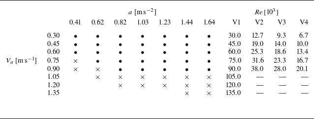


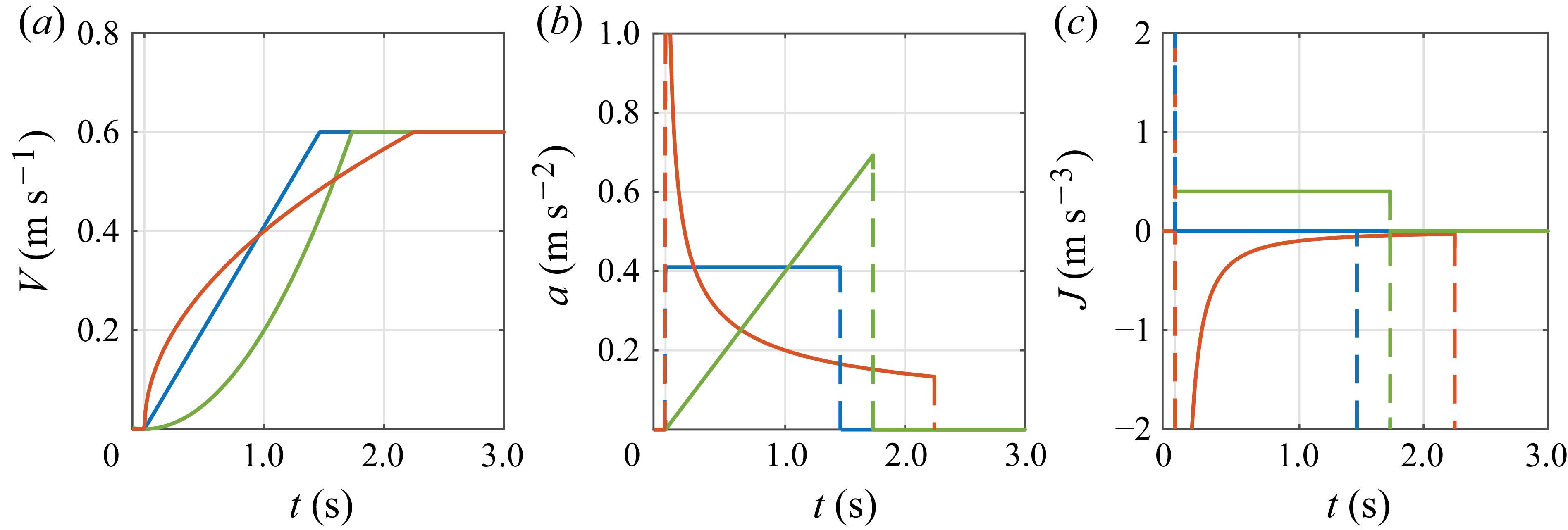


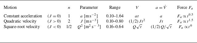


 Open access