


1. Introduction
The study of the flow past a smooth cylinder represents one of the canonical flows in fluid mechanics, being relevant for both fundamental research and engineering applications. As a result, an extended literature exists on the topic, arising from earlier experimental and numerical investigations, e.g. Tritton (Reference Tritton1959), Roshko (Reference Roshko1961), Berger & Wille (Reference Berger and Wille1972), Williamson (Reference Williamson1996) and Dong & Karniadakis (Reference Dong and Karniadakis2005). It is well established that the Reynolds number is the only parameter that drives the flow behaviour, with  $Re_D=UD/\nu$ based on the cylinder diameter $D$, the uniform inflow velocity $U$, and the kinematic viscosity $\nu$. Williamson (Reference Williamson1996) provided a comprehensive description of the different regimes. When the Reynolds number $Re_D$ is less than $47$, the flow is laminar and steady, while two-dimensional laminar vortex shedding occurs for $47 < Re_D < 180$. For Reynolds numbers in $180 < Re_D < 300$ the periodic wake becomes three-dimensional and unstable. In this transition regime, the inception of the so-called modes A and B is observed, both involving streamwise vortex structures but with distinct spanwise wavelengths. They correspond to elliptic and hyperbolic instability, respectively, with the first occurring in the primary vortex core, and the second in the saddle point region between the primary rollers; see also Roshko (Reference Roshko1954). The flow around a cylinder, as a whole, entails three shear flows: a wake flow, a mixing layer flow that separates from the lateral surfaces of the body, and a boundary layer flow on the cylinder surface (Williamson Reference Williamson1996). As $Re_D$ increases, these three shear flows become progressively unstable: first, the wake gets turbulent at approximately $Re_D>200$, then the shear layer transitions at $Re_D>1200$, and eventually the cylinder boundary layer gets unstable for $Re_D>200\,000$. At a glance: as the Reynolds number increases, a drop-down formation of smaller scales occurs, whereas the turbulent transition point moves further upstream until the boundary layer on the surface of the cylinder becomes turbulent. Whilst the flow around a uniform cylinder has been well-known since the last century, our knowledge of (even slightly) more complicated geometries turns out to be insufficient. Here, the flow around a three-dimensional stepped cylinder – namely two cylinders with different diameters joined at one extremity – is considered. The latter represents a good model for several engineering applications, e.g. aircraft landing gear and offshore wind turbine towers. The understanding of its flow dynamics is still far from being comprehensive. As an example, three different vortex shedding frequencies are identified in the wake, which is counterintuitive since one would expect just two cells (Lewis & Gharib Reference Lewis and Gharib1992). This has turned out to have relevant side effects on the structural stability of the cylinder itself.
Compared to the uniform cylinder, the flow around a single-stepped cylinder has an additional parameter to take into account, namely the ratio between the two diameters ( $r=D/d$). Performing a parametric study on $r$, Lewis & Gharib (Reference Lewis and Gharib1992) reported first a direct and indirect vortex interaction mode for the range $1.14< D/d <1.76$ at $67< Re_D<200$. The direct mode occurs when $D/d<1.25$, and it consists of two dominating shedding frequencies for the small and large cylinders, labelled $f_S$ and $f_L$, respectively. Initially in phase and connected one by one across the interface, the cells quickly move out of phase, and at least one half-loop connection between oppositely rotating vortices appears. The interruptions of one-by-one connection occur during a period called the beat cycle. For $D/d>1.55$, this interaction generates another distinct region behind the large cylinder. This is named the modulation zone by Lewis & Gharib (Reference Lewis and Gharib1992) because the velocity variation was modulated by the main frequency behind the large cylinder. They also measured the modulation frequency $f_N$. For each of the dominating shedding frequencies, Dunn & Tavoularis (Reference Dunn and Tavoularis2006) classified three main regions: the S- and L-cells behind the small and large cylinders, and the modulation N-cell with the lowest shedding frequency ( $\,f_S>f_L>f_N$). Thereafter, many authors adopted this classification (Morton, Yarusevych & Carvajal-Mariscal Reference Morton, Yarusevych and Carvajal-Mariscal2009; Morton & Yarusevych Reference Morton and Yarusevych2010; McClure, Morton & Yarusevych Reference McClure, Morton and Yarusevych2015; Tian et al. Reference Tian, Jiang, Pettersen and Andersson2017; Wang et al. Reference Wang, Ma, Wan and Yan2018; Massaro, Peplinski & Schlatter Reference Massaro, Peplinski and Schlatter2023c), which is used in the current study as well.
The interactions among the cells were studied first by Dunn & Tavoularis (Reference Dunn and Tavoularis2006) for  $D/d=2$ at $Re_D=150$ through experiments, and the results were confirmed later by Morton & Yarusevych (Reference Morton and Yarusevych2010) via Reynolds-averaged Navier–Stokes equations. At the S–N cell boundary, Morton & Yarusevych (Reference Morton and Yarusevych2010) observed a stable behaviour with a spanwise layer deflection into the large cylinder direction. The number of S–N vortex connections depends on the frequency ratio ( $\,f_S/f_N$), while the interruption of the N–S connection happens with the beat frequency $f_S-f_N$. The vortex dislocation induces half-loop connections between S-cell vortices. The concept of dislocation was introduced first by Williamson (Reference Williamson1989), who adapted the idea from a solid-mechanics mechanism. Williamson (Reference Williamson1989) described how the vorticity varies between two adjacent cells with different frequencies: first, in phase, the vortices in the cell with lower frequency are induced downstream by the high-frequency cell; then, out of phase, a contorted tangle of vortices appears across the boundary, i.e. the vortex dislocation. In the current simulations, we also observe such inclined vortical structures behind the cylinders, with a larger deflection inside the N-cell; see also Massaro, Peplinski & Schlatter (Reference Massaro, Peplinski and Schlatter2022). At the lower N–L boundary, Morton & Yarusevych (Reference Morton and Yarusevych2010) and Tian et al. (Reference Tian, Jiang, Pettersen and Andersson2017) pointed out antisymmetric features between two adjacent N-cell cycles, where, together with the L–L half-loop, there is a ‘real loop’ and a ‘fake loop’, called N–N and N–L, respectively. Morton & Yarusevych (Reference Morton and Yarusevych2010) and Tian et al. (Reference Tian, Jiang, Pettersen and Andersson2017, Reference Tian, Jiang, Pettersen and Andersson2020) focused on the laminar vortex shedding regime, and their observations seem to hold as $Re_D$ increases. Similar conclusions are drawn for the dual (Ji et al. Reference Ji, Yang, Yu, Cui and Srinil2020; Yan, Ji & Srinil Reference Yan, Ji and Srinil2020, Reference Yan, Ji and Srinil2021) and multiple (Ayancik et al. Reference Ayancik, Siegel, He, Henning and Mulleners2022) stepped cylinders. More recently, the rotating case in the laminar regime has also been studied by Zhao & Zhang (Reference Zhao and Zhang2023).
Nevertheless, these various modes and interactions need to be verified at higher Reynolds numbers, in particular when the transition to turbulence in the wake occurs. Experimentally, Norberg (Reference Norberg1992) and Ko & Chan (Reference Ko and Chan1992) measured the main integral quantities at  $Re_D=80\,000$. Morton & Yarusevych (Reference Morton and Yarusevych2014a) and Morton, Yarusevych & Scarano (Reference Morton, Yarusevych and Scarano2016) studied the wake dynamics at $Re_D=2100$, and performed tomographic particle image velocimetry investigation, respectively. Numerically, only a few studies examined the turbulent wake regime: Morton et al. (Reference Morton, Yarusevych and Carvajal-Mariscal2009) used unsteady Reynolds-averaged Navier–Stokes equations to achieve $Re_D=2000$, whereas recently, Tian et al. (Reference Tian, Jiang, Pettersen and Andersson2021) and Massaro et al. (Reference Massaro, Peplinski and Schlatter2023c) performed direct numerical simulations (DNS) at the Reynolds numbers $Re_D=3900$ and $5000$, respectively. Tian et al. (Reference Tian, Jiang, Pettersen and Andersson2021) focused on the junction region behaviour, without resolving the wake region fully. Massaro et al. (Reference Massaro, Peplinski and Schlatter2023c) analysed the spatially coherent structures arising in the fully turbulent regime, with an unsteady cylinder shear layer. The current study uses the same numerical approach as in Massaro et al. (Reference Massaro, Peplinski and Schlatter2023c). Whereas that study focused on the coherent structures of the flow at $Re_D=5000$, the focus of the present work is the lower $Re_D=1000$. We first perform a comprehensive comparison between the two regimes related to the first two shear flow instabilities, i.e. the cylinder shear layer and the wake ( $Re_D=1000, 5000$). The main part, however, will focus on the lower $Re_D=1000$. That so-called subcritical regime has not been investigated in detail before. At this Reynolds number, the cylinder shear layer is still stable, and the junction dynamics resembles that of the laminar case. The downwash appears to be dynamically significant, and by means of the proper orthogonal decomposition (POD), we detect the connection between the junction dynamics and the N-cell formation, whose origin has been debated for a long time. An explanation of the downwash mechanism behind a stepped cylinder is proposed, supported by the statistical data and modal analysis results. To limit the parameter space, a fixed diameter ratio $r=D/d=2$ is considered. However, as stated previously, Lewis & Gharib (Reference Lewis and Gharib1992) identified for the stepped cylinder geometry two distinct regimes: direct ( $r<1.25$) and indirect ( $r>1.55$) interactions. Thus the current results can be generalised for a wide range of diameter ratios, as long as an indirect interaction occurs.
In the next section, the numerical set-up and the adaptive mesh refinement (AMR) technique are introduced. Section 3 presents the two turbulent regimes at  $Re_D=1000$ and $5000$, with stable and unstable cylinder shear layers, respectively. The junction and wake dynamics are described via instantaneous vortical structures and three-dimensional statistics. The latter were collected for at least 200 small cylinder vortex shedding periods after discarding the first 400 time units ( $D/U$) to ensure proper flow development. Section 4 shows the results of the modal analysis, characterising the energy content and extension of the cells, and discussing the downwash mechanism. The connection between the POD mode 7 (and 10) and the N-cell, i.e. the relation between the downwash and the modulation cell, is described, also by considering the analytical superimposition of travelling waves. A simplified reduced-order reconstruction is used to unveil the large-scale vortex connections in the wake. Finally, the main findings and conclusions are presented in § 5.
2. Numerical framework and validation
Direct numerical simulations of the incompressible Navier–Stokes equations using the open-source code Nek5000 (Fischer, Lottes & Kerkemeier Reference Fischer, Lottes and Kerkemeier2008) are performed. In the past decades, Nek5000 has been used extensively in the computational fluid dynamics community to perform high-fidelity numerical simulations of transitional and high Reynolds incompressible flows; see, for example, El Khoury et al. (Reference El Khoury, Schlatter, Noorani, Fischer, Brethouwer and Johansson2013), Martínez et al. (Reference Martínez, Merzari, Acton and Baglietto2019), Merzari et al. (Reference Merzari, Obabko, Fischer and Aufiero2020) and Chauvat et al. (Reference Chauvat, Peplinski, Henningson and Hanifi2020). The code is based on a spectral element method (Patera Reference Patera1984) offering minimal dissipation and dispersion, high accuracy and nearly local exponential convergence. This spatial discretisation is similar to a high-order finite element method with a computational domain decomposed into non-overlapping hexahedral subdomains called elements. Each element is treated as a spectral domain with a solution spanned by the Lagrangian interpolants defined on the Gauss–Lobatto–Legendre (GLL) or Gauss–Legendre (GL) points. The  $\mathbb {P}_N-\mathbb {P}_{N-2}$ formulation is used. This corresponds to a staggered grid, where velocity and pressure are represented using $p+1$ GLL and $p-1$ GL points, respectively (where $p$ is the polynomial order). In our simulation, $p$ is set equal to $7$, as no improvement has been observed by using a higher polynomial order. The time integration is performed via third-order implicit backward differentiation, with an extrapolation scheme of order 3 for the convective term. In addition, the advection term is also over-integrated, or de-aliased, to retain its skew symmetry (Malm et al. Reference Malm, Schlatter, Fischer and Henningson2013). While collecting data, a constant time step is used to ensure a Courant–Friedrichs–Lewy number smaller than $0.4$ and capture the highest temporal frequencies.
2.1. Adaptive mesh refinement
An important extension of Nek5000 was implemented and developed by our group, namely the AMR technique (Offermans et al. Reference Offermans, Peplinski, Marin and Schlatter2020, Reference Offermans, Massaro, Peplinski and Schlatter2023; Massaro, Peplinski & Schlatter Reference Massaro, Peplinski and Schlatter2023d). The AMR technique is considered one of the relevant milestones in the future (and current) numerical simulations (Slotnick et al. Reference Slotnick, Khodadoust, Alonso, Darmofal, Gropp, Lurie and Mavriplis2014), providing significant meshing flexibility and dynamical mesh modifications during the simulation based on the instantaneous or time-averaged estimated computational error. It decreases significantly the count of computational degrees of freedom, and allows the study of flows without prior knowledge of their dynamics. The process involves the assessment of the error, with a suitable refinement criterion, and an appropriate refinement/coarsening technique. Offermans (Reference Offermans2019) introduced in Nek5000 an  $h$-type refinement, where the number of degrees of freedom is modified by splitting the entire element. In this case, an oct-tree refinement is performed, replacing a single parent element with eight (in three dimensions) children (Burstedde, Wilcox & Ghattas Reference Burstedde, Wilcox and Ghattas2011). Following Kruse (Reference Kruse1997), the conforming-space/non-conforming-mesh approach is used, where the hanging nodes are not considered as real degrees of freedom, and non-conforming interfaces are treated with an interpolation operator. Massaro et al. (Reference Massaro, Peplinski and Schlatter2023d) showed that non-conforming interfaces neither affect the solution field nor introduce any further instabilities. Appendix A provides supplemental details about the error measurement and the mesh quality assessment. In particular, it is shown that the present configuration corresponds to fully resolved DNS throughout the domain.
2.2. Problem formulation
The numerical configuration for the flow around a three-dimensional stepped cylinder is presented here. First, the set of governing equations with the corresponding initial and boundary conditions is specified. Then the geometry of the problem is described, specifying the domain sizes. The current study performs DNS of the incompressible Navier–Stokes equations, which in non-dimensional form read
 \begin{equation} \left.\begin{array}{@{}ll@{}} \boldsymbol{\nabla}\boldsymbol{\cdot} \boldsymbol{u} = 0, \\ \displaystyle \dfrac{\partial \boldsymbol{u} }{\partial t} + \left( \boldsymbol{u} \boldsymbol{\cdot} \boldsymbol{\nabla} \right) \boldsymbol{u} ={-} \boldsymbol{\nabla} P + \dfrac{1}{Re_D}\, \nabla^2 \boldsymbol{u}, \end{array} \right\} \end{equation}
where  $\boldsymbol {u}$ is the non-dimensional velocity vector, $P$ is the non-dimensional pressure, and $Re_D=UD/\nu$ is the Reynolds number based on the cylinder diameter $D$, the uniform inflow streamwise velocity component $U$, and the kinematic viscosity $\nu$. The set of equations is incomplete without proper initial and boundary conditions. In our set-up, the initial condition is a uniform distribution of the streamwise velocity with unitary value $\boldsymbol {u}(\boldsymbol {x},t_0)=(1,0,0)$, which, however, adapts quickly to a more physical solution. At the inflow, the same is set as a Dirichlet boundary condition $\boldsymbol {u}(\boldsymbol {x},t_0)=\boldsymbol {u}(\boldsymbol {x}_0,t)=(1,0,0)$. The outflow consists of natural boundary condition $(-p \boldsymbol {I} + \nu \,\boldsymbol {\nabla } \boldsymbol {u})\boldsymbol {\cdot } \boldsymbol {n} = 0$, where $\boldsymbol {n}$ is the normal vector. We focus on the junction and wake dynamics, rather than considering the end-plate effects. Thus our top/bottom boundary conditions assume an infinitely long cylinder, prescribing symmetry boundary conditions $\boldsymbol {u} \boldsymbol {\cdot } \boldsymbol {n} = 0$ with $(\boldsymbol {\nabla } \boldsymbol {u} \boldsymbol {\cdot } \boldsymbol {t}) \boldsymbol {\cdot } \boldsymbol {n}= 0$, where $\boldsymbol {t}$ is the tangent vector. For the front and back boundaries, mixed conditions are used, similar to the open boundary at the outflow, but prescribing zero velocity increment in non-normal directions. The stepped cylinder surface has a no-slip and impermeable wall.
The stepped cylinder presents two cylinders of different diameters joined at one extremity, with a ratio  $D/d=2$ ( $D=1$). An infinitely long cylinder is considered, using the boundary conditions discussed above. We have devised a configuration akin to that in Morton & Yarusevych (Reference Morton and Yarusevych2014b), in order to corroborate our findings through comparison with prior experiments. The stepped cylinder is located at the origin of the Cartesian frame oriented with the $z$-axis on the cylinder. The large and small cylinders span vertically for 10 and 12 diameters $D$, respectively. The computational box is a parallelepiped with extension $(-10D,30D)$ in $x$,
$x$,  $(-10D,10D)$ in $y$, and $(-10D,12D)$ in $z$, where $x,y,z$ are the streamwise, lateral and vertical (or spanwise) directions, respectively (see figure 1). To prevent any undesired side and boundary effects, the domain has been designed carefully. In the planning phase, tests were conducted to monitor closely both local and global quantities while varying the domain sizes. Furthermore, the implementation of the AMR technique allows for the usage of a substantially larger domain while ensuring DNS-like resolution. For more details, refer to Appendix A.
2.3. Consistency with experimental measures
Not many reference data of high quality exist for the present flow case. In order to verify the accuracy of our numerical configuration, local and integral measures were compared with experiments from Morton & Yarusevych (Reference Morton and Yarusevych2014b) and Roshko (Reference Roshko1961).
First, the spectral analysis of velocity signals is used to determine the vortex shedding frequency and investigate how it varies with the spanwise location. Five virtual velocity probes are placed at the same locations as in Morton & Yarusevych (Reference Morton and Yarusevych2014b). The time signals are acquired with the sampling frequency  $f D/U = 100$. The Nyquist theorem requirements are definitely met since the highest frequency of the flow is expected to be the small cylinder vortex shedding at $f_s D/U \approx 0.4$. The time interval is long enough to capture the slowest dynamics exploring over approximately $200$ S-cell vortex shedding periods. The virtual probes have identical streamwise and lateral locations ( $x=5D$ and $y=0.75D$), but different spanwise locations: $z_1=4D$, $z_2=-1D$, $z_3=-3D$, $z_4=-5D$ and $z_5=-9D$. At these positions, the power spectral density (PSD) of the streamwise velocity component is computed. The results are in excellent agreement with the measurements by Morton & Yarusevych (Reference Morton and Yarusevych2014b); see table 1. For each cell, a single peak is evident with a high energy content ( $z_1, z_3, z_5$). At the upper (S–N) and lower (N–L) interfaces, a double peak appears. Here, the PSD highlights the interaction between two different shedding frequencies, and the twofold hills have a lower energy content; see figure 2(b).
Strouhal numbers for different probe locations. The results from the current study and the experiments by Morton & Yarusevych (Reference Morton and Yarusevych2014b) are reported in the first and second rows, respectively.

Sketch of the three-dimensional stepped cylinder with planar cross-sections at  $z=0$ and $x=0$. The frame of reference and the dimensions of the domain are reported. The black arrows indicate the uniform inflow with streamwise velocity $U$. The figure is adapted from Massaro et al. Reference Massaro, Peplinski and Schlatter2023c.

Logarithmic plot of power spectral density (PSD) of the streamwise velocity component at locations (a)  $z_1=4D$, (b) $z_2=-1D$, (c) $z_3=-3D$, and (d) $z_5=-9D$. The green circles indicate the double peak at the N–L interface. The time signals are acquired with the sampling frequency $f D/U = 100$, for at least $200$ S-cell vortex shedding periods.

The frequency peak is used to calculate the Strouhal number, defined as  $St=fD/U$. The frequency $f$ at the specific location and the unitary inflow velocity $U$ are considered. Once again, the agreement with the experimental measurements is excellent. Each wake region is characterised by a distinct shedding frequency and exhibits a single peak: $St_S=0.408$, $St_N=0.188$ and $St_L=0.201$ for the S-, N- and L-cells, respectively. At the S–N boundary ( $z_2$), the two dominant peaks are related to the Strouhal numbers of each of the adjacent cells. Analogously, a double peak at the N–L boundary is observed. Morton & Yarusevych (Reference Morton and Yarusevych2014b) use the streamwise velocity spectra to analyse how the energy content varies in the different cells and the extension of the cell. Analogous conclusions can be drawn in this scenario: at the interface in figure 2(b), the energy content is diminished substantially compared to that within the single cells; see figures 2(a,c,d). Nevertheless, a more detailed discussion about the energy content for each cell is carried out in the POD section.
When studying the flow around a bluff body, the pressure and drag coefficients are useful integral indicators. Thus the estimated mean value and variance of the drag for each cylinder are computed. The dimensionless drag coefficient  $c_D$ is defined as the component of the aerodynamic force aligned with the inflow flow (here horizontal) and normalised with $(1/2)\rho U^2 D L_z$, with $L_z$ being the vertical cylinder length. Then it is averaged in time to yield $\bar {c}_D$. The aerodynamic force components along the $y$ and $z$ directions are computed as well. For symmetry reasons, the lateral $y$ component of the coefficient $\bar {c}_y$ is expected to approach zero. In the current study, the results are $\bar {c}_{y_S}=0.0017$ and $\bar {c}_{y_L}=0.00053$, for the small and large cylinders, respectively. This assesses the good temporal convergence of our statistics for any integral quantities. When it comes to the $z$-averaged mean drag coefficients, the results are $\bar {c}_{D_S}=1.1084$ and $\bar {c}_{D_L}=0.9083$. The standard deviation of both signals is small, with value $\sigma _{c_D} \approx 0.016$. As predicted by Roshko (Reference Roshko1961), in the Reynolds number range $100< Re_D<10^5$, the drag coefficient is $c_D\approx 1$. Now the viscous and pressure contributions to the overall drag are computed. For both cylinders, the pressure term is dominant (approximately $90\,\%$) with respect to the viscous one, but the viscous component is slightly larger for the small cylinder, where $\bar {c}_{Dv} \sim 12.7\,\%$ instead of $\bar {c}_{Dv} \sim 9.6\,\%$. Because previous studies did not provide $c_D$ estimations at this specific Reynolds number and did not analyse individually drag contributions from the small and large cylinders, we undertake a comparison with the outcomes of the uniform cylinder by Roshko (Reference Roshko1961). The results are in good agreement, with integral difference less than 5 %. As expected, the junction does not affect substantially the integral drag values. However, as we will explore in the following sections, this is not true for three-dimensional time-averaged statistics, particularly in the near-wake area.
3. The evolution of the turbulent flow
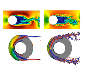
In the current section, the main features of turbulent flow around a single-stepped cylinder are described. After conducting a set of three simulations that represent different regimes, as shown in figure 3, we turn our attention to the turbulent wake regime. More precisely, the stepped cylinder with both a stable ( $Re_D=1000$) and unstable ( $Re_D=5000$) cylinder shear layer is studied, as the laminar vortex shedding ( $Re_D=150$) was investigated thoroughly in previous works (Lewis & Gharib Reference Lewis and Gharib1992; Dunn & Tavoularis Reference Dunn and Tavoularis2006; Morton & Yarusevych Reference Morton and Yarusevych2010).
Different regimes of the flow around a stepped cylinder: (a) the laminar vortex shedding at  $Re_D=150$, and the turbulent wake with a (b) stable and (c) unstable shear layer at $Re_D=1000$ and $Re_D=5000$, respectively. Isosurfaces of the velocity magnitude in the $xy$ ( $z=0$) plane.

3.1. Characterisation of the junction region
Looking at the instantaneous vortical structures, we first focus on the junction region, i.e. the flat surface with sharp edges that joins the two cylinders. Aware that an unequivocal definition for a fundamental structure as the vortex does not yet exist (Cucitore, Quadrio & Baron Reference Cucitore, Quadrio and Baron1999), we rely on the  $\lambda _2$ criterion by Jeong & Hussain (Reference Jeong and Hussain1995) to identify organised and coherent structures in the flow. The $\lambda _2$ definition corresponds to connected planar regions of pressure minimum, discarding the contributions of unsteady irrotational straining and viscous terms in the Navier–Stokes equations. An adequate normalisation is taken into account, and from now on each $\lambda _2$ value is normalised by $U^2/D^2$. The structures’ classification follows the convention by Massaro et al. (Reference Massaro, Peplinski and Schlatter2023c).
At  $Re_D=1000$ (figure 4a), on the front of the junction, the impingement of the flow, due to the presence of the small cylinder, together with the leading edge separation, is mainly responsible for the horseshoe vortex H1 formation. By definition, the horseshoe vortex consists of a trio of interconnected vortices (Dargahi Reference Dargahi1989). These comprise a bound vortex encircling the small cylinder, along with two trailing vortices that stretch from the bound vortex into the wake area. The consequent recirculating bubble has the time-averaged pressure minimum at $(x,y,z)=(-0.354D,0D,0.046D)$. In addition, the blockage and the H1 rotation induce the incoming flow to divert laterally, where it spills over the edges of the step. Here, it rolls up into two streamwise edge vortices E, similar to the tip vortices on the free-end surface of a finite-length cylinder (Zdravkovich et al. Reference Zdravkovich, Brand, Mathew and Weston1989). These observations agree with the measurements first made by Dunn & Tavoularis (Reference Dunn and Tavoularis2006) at $Re_D=150$ and with the hydrogen bubble visualisations by Morton & Yarusevych (Reference Morton and Yarusevych2014b) at $Re_D=1000$. Recently, Tian et al. (Reference Tian, Jiang, Pettersen and Andersson2021) has pointed out some additional structures, confirmed by Massaro et al. (Reference Massaro, Peplinski and Schlatter2023c). In the laminar front part of the junction, they observe two horseshoe vortices, H3 and H4, with H4 appearing upstream of H3, and rotating in the same direction as H1. At $Re_D=1000$, the configuration is different. Figure 4(a) shows clearly that the horseshoe vortices H3 and H4 do not appear, and the leading edge separation generates only H1. This leads to a crucial difference in the E formation mechanism. As long as the cylinder shear layer remains stable, the process that generates the edge vortices agrees with the Dunn & Tavoularis (Reference Dunn and Tavoularis2006) observations at lower $Re_D=150$. The leading edge separation with the small cylinder impingement drives the recirculating vortex H1 formation that laterally deviates the incoming flow shaping the E. Furthermore, no hairpin vortices (HP) appear at $Re_D=1000$. On the other hand, a train of hairpins is clearly visible in figure 4(b), and their cyclic dynamics is described by Massaro et al. (Reference Massaro, Peplinski and Schlatter2023c). The second kind of structure reported by Tian et al. (Reference Tian, Jiang, Pettersen and Andersson2021) is named H2. Interestingly, this is present also at the current $Re_D=1000$ (figure 4). Less dynamically relevant, since it evolves at the base of the small cylinder and does not interact with other structures, this horseshoe vortex has a cross-flow width that continues to increase downstream, as for H1. The H2 structure is induced by the downward flow separation along the small cylinder wall, as confirmed by the time-averaged vertical velocity in figure 5. It is understandable that Morton & Yarusevych (Reference Morton and Yarusevych2014b) do not report these structures due to the challenges of handling hydrogen bubbles on the junction. More surprisingly, this vortex has not been classified before at lower Reynolds numbers (Vallès, Andersson & Jenssen Reference Vallès, Andersson and Jenssen2002; Dunn & Tavoularis Reference Dunn and Tavoularis2006; Tian et al. Reference Tian, Jiang, Pettersen and Andersson2020). Nevertheless, the downward flow separation along the small cylinder is not associated with the turbulent character of the flow, and H2 structures are expected to be observed at lower $Re$ as well. Simulating all three different flow regimes, and guaranteeing a well-resolved mesh around the junction with the AMR, the presence of H2 is confirmed. Based on the overall view, we assert that this is a common feature for all three flow regimes.
Top view of instantaneous  $\lambda _2$ structures around the junction: isocontours of $\lambda _2$ coloured with the streamwise vorticity for (a) $Re_D=1000$ ( $\lambda _2 =-4 U^2/D^2$) and (b) $Re_D=5000$ ( $\lambda _2 =-40 U^2/D^2$). The horseshoe and hairpin vortices are indicated (H1, H2, H3, H4 and HP), along with the edge (E) and ring (R) vortical structures. In the circle, the E vortex rolling up around the edge and splitting is highlighted.

Time-averaged vertical velocity component in the  $xz$ ( $y=0$) and $xy$ ( $z=0$) planes at(a) $Re_D=1000$ and (b) $Re_D=5000$.

All these vortices are stable and with only small fluctuations in time, as they develop in the laminar/transitional part of the flow. On the contrary, the back structures are weaker and more difficult to identify since they are placed in the turbulent wake of the small cylinder. This makes them almost indistinguishable from the small turbulent eddies. However, the heads of the two streamwise base vortices that begin to develop on the back part of the junction are identified; see also Massaro et al. (Reference Massaro, Peplinski and Schlatter2022). Furthermore, the  $\lambda _2$ structure named ring R vortex points out the recirculation occurring at the trailing edge and is reported here for the first time. This structure is weaker than H1 and with a different formation mechanism: the E vortices roll up around the edges and split before diverging laterally; see figure 4(a). The low-pressure region behind the cylinder stabilises R on the back, whereas the strong downstream advection interrupts the ring connection laterally. At $Re_D=5000$, the ring vortex is not observed (independently on the $\lambda _2$ threshold) as the hairpins interaction modifies the flow topology substantially.
The analysis of time-averaged statistical quantities supports the description of the main junction mechanisms. In particular, figure 5 shows the vertical velocity component  $\bar {W}$. On the forepart of the $xz$ plane, the leading edge separation at $x=-0.5D$ is in red, and the downward flow separation along the small cylinder wall is in blue. In the $xy$ plane, a symmetric behaviour is observed for positive and negative $y$: an upward flow induced by H1 surrounded by the downward flow separation along the small cylinder and the edge H2 induced flow. A larger number of structures at $Re_D=5000$ leads to a more complicated statistical footprint. This is always the case when an obstacle interacts with a wall, namely the small cylinder with the junction. Nevertheless, it is remarkable that these interactions are observed on such a narrow surface with only $0.25D$ radial widths; see figure 5(b). The $xy$ plane confirms the structures’ evolution detected above: the H3 appearance only at higher Reynolds numbers, and the E formation mechanism being $Re_D$-related.
3.2. Characterisation of the wake
As the Reynolds number increases, the wake becomes more intricate, and numerous turbulent eddies emerge in a range that varies from the cylinder diameter to the Kolmogorov scale. The increasing complexity is clearly visible in figure 6. At  $Re_D=1000$, despite the turbulent wake behaviour, the vertical vortices with $z$-oriented axis are still visible. Superposed, smaller streamwise spaghetti-like structures are observed; see figure 6(a). In laminar vortex shedding, the $z$ vortices are distinguishable, making the vortex dislocations simple to track (Tian et al. Reference Tian, Jiang, Pettersen and Andersson2020). This is definitely not the case for a turbulent wake. Nevertheless, at the S–N boundary, the occurrence of the dislocation is still visible since the boundary is characterised by two largely different frequencies and is thus stable. Figure 6(a) shows the breaking of the initial in-phase vortex shed by the cylinder, and the consequent dislocation. The oblique shedding occurs in the modulation region with the dislocation at its boundary (Massaro et al. Reference Massaro, Peplinski and Schlatter2022). Contrary to the upper interface, the N–L layer is unstable, and dislocation detection is not possible. At the highest Reynolds number, the situation worsens even further; see figure 6(b). Massaro et al. (Reference Massaro, Peplinski and Schlatter2023c) characterise the wake of the latter case: secondary spanwise vortices appearing behind the small cylinder (caused by a Kelvin–Helmholtz instability), spanwise vortices stack organisation with the appearance of small- and large-scale braids (see figure 5 in Massaro et al. Reference Massaro, Peplinski and Schlatter2023c). Previous works developed different techniques to study the wake dynamics, e.g. for obtaining the phase and the shed position of vortices (Tian et al. Reference Tian, Jiang, Pettersen and Andersson2020). Due to the inherent complexity of turbulence, these methods, valid at lower Reynolds numbers, no longer hold. In the next section, a different approach is proposed, using the modal analysis to identify the energy content and the extension of the cells, and to study the large-scale vortex connections.
Instantaneous  $\lambda _2$ structures coloured with the vertical vorticity component in the wake at (a) $Re_D=1000$ ( $\lambda _2 =-4 U^2/D^2$) and (b) $Re_D=5000$ ( $\lambda _2 =-40 U^2/D^2$), where (b) is adapted from Massaro et al. (Reference Massaro, Peplinski and Schlatter2023c).

Due to the turbulent nature of the wake, analysing its three-dimensional time-averaged statistics can guide us in distinguishing between the subcritical ( $Re_D=1000$) and fully turbulent ( $Re_D=5000$) regimes. As expected, the wakes of both the small and large cylinders exhibit similarities to the uniform cylinder wakes far away from the junction. Nevertheless, significant differences are noticeable in the region below the junction, which extends to a considerable distance of 4–5 times the diameter of the large cylinder. The time-averaged streamwise velocity component in the $xz$ planes ( $y=0$) points out distinctly different extensions of the recirculation; see figure 7(a). At $Re_D=1000$, the negative $\bar {U}$ region extends for $0.63D$ and $2.43D$ behind the small and large cylinders, respectively. In the case of the larger cylinder, the recirculation gets stronger inside the N-cell. Qualitatively, this is clear from the more intense blue colour in figure 7(a). This is a meaningful characteristic of the modulation area only, and the connection with the downwash mechanism is discussed below. Quantitatively, albeit the trend of the streamwise velocity $\bar {U}$ does not vary for the two Reynolds numbers, the backflow phenomenon is more intense at $Re_D=5000$. The peak reaches 40 % of the inflow velocity, with the minimum occurring at a lower vertical location; see figure 7(b). Likewise, figure 7(c) shows that at higher Reynolds numbers, the mean vertical velocity $\bar {W}$ exhibits significantly more negative values. Despite the differences in the wake characteristics, the same trend is observed at distance approximately $5D$ from the cylinder (figure 7). Specifically, the wake profile begins to resemble that of a uniform cylinder at this point, regardless of the Reynolds number. This suggests that the extension of the N-cell structure, which is responsible for the oblique periodic shedding of vortices, is not affected significantly by changes in the Reynolds number and the transition of the cylinder shear layer. This is also confirmed by the POD results in the next section. Eventually, the variation in the vortex formation length is worth noting and deserves further discussion as it plays a crucial role in the dynamics of the wake.
(a) Time-averaged streamwise velocity component in the  $xz$ plane at $y=0$ for $Re_D=1000$. The black dashed lines indicate the locations where the data are extracted for (b,c), corresponding to $z=0D$ (black), $z=-2D$ (blue), $z=-4D$ (green) and $z=-8D$ (red). The time-averaged (b) streamwise and (c) vertical velocity components are plotted at different spanwise locations. Both velocity components are normalised by the inflow velocity $U$. The solid and dashed lines refer to $Re_D=1000$ and $Re_D=5000$, respectively.

The spanwise variation of the vortex formation length refers to the change in the distance between the consecutive vortex shedding points in the wake, as we move along the spanwise direction. This variation can lead to the development of different modes of vortex shedding, which can affect the wake structure and its associated aerodynamic properties. Therefore, understanding the spanwise variation of the vortex formation length is essential to gain insight into the wake dynamics and its impact on the flow field. In the current study, the location of the maximum streamwise velocity fluctuation  $\overline {uu}$ is used to define the vortex formation length (Norberg Reference Norberg1998; Govardhan & Williamson Reference Govardhan and Williamson2001). The vortex formation lengths behind the small cylinder for two different $Re_D$ values are observed to match well, with a noticeable reduction inside the N-cell region; see figure 8. Specifically, decreases of approximately 20 % and 15 % are measured at $Re_D=1000$ and $Re_D=5000$, respectively. This contraction has a significant connection with the downwash phenomenon, as discussed below. Indeed, the reduction in vortex formation length leads to a decrease in the distance between the vortices shed by the cylinder. This, in turn, creates a larger wake deficit, which has a substantial impact on the aerodynamic forces experienced by the cylinder.
Spanwise variation of the vortex formation length for Reynolds numbers  $Re_D=1000$ and $5000$.

In summary, the two turbulent regimes at  $Re_D=1000$ and $Re_D=5000$ present similar characteristics far away from the junction, where the wake resembles the uniform cylinder shape. The reduction of the vortex formation length inside the N-cell is also consistent. However, the ratio between the frequencies of N- and L-cells tends to diverge with the Reynolds number (Massaro et al. Reference Massaro, Peplinski and Schlatter2023c). The localised and stronger vertical velocity flux inside the modulation region at $Re_D=5000$ (with more intense $\overline {ww}$; see figure 9 in Massaro et al. Reference Massaro, Peplinski and Schlatter2023c) is the consequence of a less energetic downwash phenomenon behind the junction. Therefore, the instability of the cylinder shear layer results in an increase of the energy content for the modulation cell, in agreement with the trend of the POD spectrum (see figure 10 in Massaro et al. Reference Massaro, Peplinski and Schlatter2023c). As discussed below, the POD identifies the three cells as the most energetic structure, in agreement with the statistical analysis for both $Re_D$ values. Nevertheless, a remarkable difference in the downwash dynamics is observed between the stable and unstable shear layer cases.
4. Modal analysis of the subcritical regime
The detection of the three different cells in the turbulent wake can be achieved by modal decomposition. In particular, the POD is used to extract the most energetic spatially coherent structures. For both Reynolds numbers, they coincide with L-, S- and N-cells. However, at  $Re_D=1000$, i.e. a turbulent wake with a stable shear layer as the gateway (which has not been documented previously), one of the POD modes reveals the downwash dynamics in a prominent way. In the current section, first the POD formulation and the assessment of its convergence are described, with the introduction of a novel criterion adapted from spectral proper orthogonal decomposition (SPOD). Then the downwash dynamics is described, by establishing a simplified analytical description and reconstructing a reduced-order representation of the flow to study the large-scale vortex connections.
4.1. Theoretical formulation
Given a set of  $m$ snapshots $\boldsymbol {u}_j$, with $j=0,\ldots,m-1$, these are assembled in the snapshot matrix $\boldsymbol{\mathsf{U}}_m$:
 \begin{equation} \boldsymbol{\mathsf{U}}_m = [\boldsymbol{u}_0, \boldsymbol{u}_1,\ldots,\boldsymbol{u}_{m-1}] \in \mathbb{R}^{n \times m}, \end{equation}
where  $n$ is the total number of grid points multiplied by the number of velocity components. The modal analysis allows us to split the system into space- and time-dependent parts. In this regard, the POD is employed (Berkooz, Holmes & Lumley Reference Berkooz, Holmes and Lumley1993). The POD performs the modal decomposition of the nonlinear flow minimising the residual energy between the snapshots and their reduced linear representation. They are constructed to be the orthogonal basis that represents the optimal projection, in energy terms, of the most important dynamical features. It was first introduced in the fluid mechanics context by Lumley (Reference Lumley1970), and is usually named classical POD. Here, the snapshot POD is used, developed by Sirovich (Reference Sirovich1987) to handle the analysis of three-dimensional flows with a large set of grid points. The notation adopted in the following derivation follows Sarmast et al. (Reference Sarmast, Dadfar, Mikkelsen, Schlatter, Ivanell, Sørensen and Henningson2014).
When assembling the snapshots matrix, the collected snapshots are sampled according to the Nyquist criterion ( $\Delta t =0.25 D/U$) and collected for an interval that is sufficiently long to embed the slowest frequency. As indicated in (4.1), the set of $m$ snapshots $\boldsymbol {u}_j$ is rearranged in the snapshot matrix $\boldsymbol{\mathsf{U}}_m$. The orthogonal basis function $\boldsymbol {X}$ and the corresponding time coefficients $\boldsymbol {T}$ are computed via the singular value decomposition of the snapshot matrix as
 \begin{equation} \boldsymbol{\mathsf{U}}_m = \boldsymbol{X} \boldsymbol{T} = \boldsymbol{X} \boldsymbol{\varSigma} \boldsymbol{\mathsf{W}}, \end{equation}
where  $\boldsymbol {T} = \boldsymbol {\varSigma } \boldsymbol{\mathsf{W}}$, with $\boldsymbol{\mathsf{W}}$ being the matrix of the right singular vectors, and $\boldsymbol {\varSigma } \in \mathbb {R}^{n\times m}$ the matrix of singular values of $\boldsymbol{\mathsf{U}}_m$ (i.e. the energies). To guarantee the unit energy of each mode, the proper normalisation has to be taken into account: $\| \boldsymbol {X} \|_{{M}} = \boldsymbol{\mathsf{I}}$ and $\| \boldsymbol{\mathsf{W}} \|_{{N}} = \boldsymbol{\mathsf{I}}$, where $\boldsymbol{\mathsf{M}} \in \mathbb {R}^{n\times n}$ and $\boldsymbol{\mathsf{N}}\in \mathbb {R}^{n\times n}$ are the mass and the temporal weight matrix, respectively, and $\boldsymbol{\mathsf{I}}$ is the identity matrix. If the snapshots are collected with equidistant time intervals, then $\boldsymbol{\mathsf{N}}=\boldsymbol{\mathsf{I}}$. The above normalisation is obtained by considering $\boldsymbol{\mathsf{M}}^{1/2} \boldsymbol{\mathsf{U}}_m \boldsymbol{\mathsf{N}}^{1/2}$ and computing
 \begin{equation}
\boldsymbol{\mathsf{M}}^{1/2}
\boldsymbol{\mathsf{U}}_m \boldsymbol{\mathsf{N}}^{1/2} =
\hat{\boldsymbol{\mathsf{X}}} \boldsymbol{\varSigma}
\hat{\boldsymbol{\mathsf{W}}}, \end{equation}
\begin{equation}
\boldsymbol{\mathsf{M}}^{1/2}
\boldsymbol{\mathsf{U}}_m \boldsymbol{\mathsf{N}}^{1/2} =
\hat{\boldsymbol{\mathsf{X}}} \boldsymbol{\varSigma}
\hat{\boldsymbol{\mathsf{W}}}, \end{equation}
where  $\hat {\boldsymbol{\mathsf{X}}}$ and $\hat {\boldsymbol{\mathsf{W}}}$ are unitary matrices: $\hat {\boldsymbol{\mathsf{X}}}^{\rm T} \hat {\boldsymbol{\mathsf{X}}} =\boldsymbol{\mathsf{I}}$ and $\hat {\boldsymbol{\mathsf{W}}}^{\rm T} \hat {\boldsymbol{\mathsf{W}}} =\boldsymbol{\mathsf{I}}$.
Eventually, the modes are reconstructed as  $\boldsymbol {X} = \boldsymbol{\mathsf{M}}^{-1/2} \hat {\boldsymbol{\mathsf{X}}}$, with unit energy and orthogonal to each other, while the time coefficients are $\boldsymbol {T} = \boldsymbol {\varSigma } \boldsymbol{\mathsf{W}}^{\rm T}$, where the energies are given by the diagonal matrix $\boldsymbol {\varSigma }$.
4.2. Convergence criterion
Before discussing the modal analysis results, the POD convergence is assessed and the set of snapshots is guaranteed to be adequately large. To this end, first the energy spectrum for progressively larger  $m$ is computed, and then the correlation coefficient is estimated for two different snapshot sets. To improve the convergence of the decomposition, the $y$-symmetry of the stepped cylinder is exploited, resulting in a statistical symmetry for the flow (Berkooz et al. Reference Berkooz, Holmes and Lumley1993). In figure 9, the spectrum is computed for progressively larger data sets, from $m=1200$ to $m=2400$ snapshots. The last three cases (with $m=1800,2000,2400$) show excellent agreement for the first four modes. Starting with modes 5 and 6, the blue line ( $m=1200$) deviates from the others. Contrary to these, the azure ( $m=2000$) and black ( $m=2400$) curves nearly overlap, especially for $j \leqslant 200$. As the POD orders the modes based on their fluctuating energy levels, we observe that the spectra of the first $200$ energetically relevant modes do not show significant deviations. In addition, good agreement between mode 0 (which corresponds to the expected mean value according to our notation) and the correspondent mean flow (estimated via statistical analysis in Massaro et al. 2023, personal communication) is appreciated.
The POD spectrum with the percentage energy contribution: (a) first  $500$ and (b) first $20$ modes are shown. Different numbers of snapshots $m$ are considered. The orange dashed ellipses and solid circle indicate the three most energetic travelling modes and the downwash mode (single point), respectively.

To corroborate previous qualitative observations, a quantitative estimation of the POD convergence is performed by dividing the data sets into two blocks ( $A$ and $B$), with a minimum of $10$ % overlapping. On each subset, the POD is carried out, and the correlation between the sets is computed. The criterion is adapted from previous works (Lesshafft et al. Reference Lesshafft, Semeraro, Jaunet, Cavalieri and Jordan2019; Abreu et al. Reference Abreu, Tanarro, Cavalieri, Schlatter, Vinuesa, Hanifi and Henningson2021) where the SPOD is used. Thus some adjustments are required. Let us consider the pair of modes $i$-
$i$- $j$: they represent a unique travelling mode where the mode $j$ is the same mode $i$ with a 90-degree phase shift. For the two sets of snapshots $A$ and $B$, the travelling modes are $\varPhi _{ij}$ and $\hat {\varPhi }_{ij}$, respectively:
 \begin{gather} \varPhi_{ij} = {\rm Re} \left\{ \phi_i + \mathrm{i} \phi_j \right\}, \end{gather}
 \begin{gather}\hat{\varPhi}_{ij} = {\rm Re} \left\{ (\phi_i + \mathrm{i} \phi_j)\,{\rm e}^{\mathrm{i} \theta} \right\}, \end{gather}
where  $\mathrm {i}$ is the imaginary unit, and the indices $i$ and $j$ refer to the POD mode number. The angle $\theta$ is needed to take into account the possible phase variation between $\varPhi$ and $\hat {\varPhi }$, as explained below. At this point, the correlation coefficient is introduced for a travelling mode $p$, made of two modes $i$ and $j$:
$j$:
 \begin{equation} \rho_{p} = \frac{ \left \langle \varPhi_{ij} \hat{\varPhi}_{ij} \right\rangle }{\| \varPhi_{ij} \| \| \hat{\varPhi}_{ij} \|}, \end{equation}
e.g. the first travelling mode has  $p=1$ with $i=1$ and $j=2$. Since the travelling modes $\varPhi _{ij}$ and $\hat {\varPhi }_{ij}$ arise from different snapshots, they have many different orientations in the complex plane, and the possible phase shift has to be taken into account. Thus $\hat {\varPhi }$ is multiplied by ${\rm e}^{\mathrm {i} \theta }$, with $\theta$ varying between 0 and $2{\rm \pi}$. When they are aligned, their correlation is going to be maximum. The phase difference varies among the travelling modes as reported in table 2.
Correlation coefficient  $\rho _p$ for all the main pairs $p$ of POD modes $i$-
$i$- $j$. In the last column, the phase shift $\theta$ for the travelling mode $p$ is computed from two sets of snapshots.

When the correlation coefficient is close to unity, the POD convergence is achieved. For the first two pairs, the correlation is higher than  $95\,\%$. Interestingly, the second pair has better convergence than the first. This can be explained by the fact the travelling mode 2-3 is related to the small cylinder, which has a vortex shedding frequency two times larger than the other frequencies. Consequently, for the same period $T$, double the number of vortices are shed. Considering the modulation region modes (5-6), even they show good convergence: $\rho _{p}>0.87$. This criterion does not apply to single mode 7, which is discussed below. Even the next pair, $8$-
$8$- $9$, is highly correlated, indicating that the first ten modes are converged adequately ( $\rho _{p}>0.87$) given the collected number of snapshots.
4.3. The most energetic structures
We begin by presenting the most relevant structures extracted via POD of the flow. They correspond to three main travelling modes in the streamwise direction; see figure 10. Each of them consists of a pair of modes with a  $90$-degree phase shift, which characterises the L-, S- and N-cells, respectively. They are all made symmetric with respect to the $y$-axis, reflecting the inherent $y$-symmetry of the flow.
Isosurfaces of the velocity magnitude  $0.1U$ for the (a) first, (b) third and (c) fifth POD modes at arbitrary phase. The second, fourth and sixth modes correspond to the phase-shifted versions of the shown modes. Dashed lines indicate the corresponding cells, and the solid ellipse highlights the S vortical structures deflection. Dotted lines point out the N-cell contraction in the streamwise direction.

The first pair of modes (1 and 2) corresponds to the large cylinder structures in the L-cell. Their energy contribution is estimated by computing the fraction  $\lambda _j/\sum _{j>0}\lambda _j$, where $j$ is the mode index, and $\lambda$ is the singular value for mode $j$. They account for approximately ${\sim }7.5\,\%$ of the total (fluctuating) energy each. This means that the coherent structures behind the large cylinder (and below the modulation region) give an overall energy contribution of ${\sim }15\,\%$. The S-cell of the small cylinder is characterised by the second travelling mode 3-4, overall as counting for ${\sim }11\,\%$. It is noticeable that the small cylinder dynamics (with $Re_d = Re_D/2$) still has a significant energy contribution. The modulation region pair is formed by modes $5$ and $6$, whose contribution is half of the previous couple, i.e. ${\sim }2.8\,\%$, in total ${\sim }5.6\,\%$.
Morton & Yarusevych (Reference Morton and Yarusevych2014b) measure the extension of the cells using hydrogen bubble visualisations. The qualitative description of the flow carried out in § 3 through  $\lambda _2$ structures corroborates their observation. In addition, the extracted POD modes allow us to define the spatial extension of each cell in a quantitative way for the turbulent regime. Indeed, each of the most energetic POD modes corresponds to a specific cell as it holds no value beyond the regions outlined below. The S region spreads behind the small cylinder and slightly below the $xy$ centre plane, at $z\approx - 0.5D$; see figure 10. On the other side, the large cylinder modes (1-2) extend for $z<-5D$. Regarding the N-cell, Dunn & Tavoularis (Reference Dunn and Tavoularis2006) observed a non-constant vertical extension in the streamwise direction. In particular, at the laminar Reynolds numbers $Re_D=150$ and $152$, this is also reported by Morton & Yarusevych (Reference Morton and Yarusevych2010). It is worth noting that such a contraction is persistent in the turbulent regime and depicted by the fifth mode in figure 10(c). The spatially coherent structure of the N-cell has a width that varies with streamwise location. In particular, the upper and lower envelope of the cell contract proportionally to $y_{up} \sim -0.1x$ and $y_{low} \sim 0.15x$, respectively. Moreover, the modulation region develops only behind the large cylinder $-0.5D< z<-4.5D$. At first glance, this may appear counterintuitive since one would expect that the intermediate region is straddling the junction, rather than being only behind one of the cylinders. A possible explanation and its connection with the downwash mechanism are discussed below. At the same time, between cells, the vortex dislocation mechanism by Williamson (Reference Williamson1989) occurs: the vortices in the cell with lower frequency are induced downstream by the high-frequency cell; see N–L interaction. That is not the case for the N–L boundary since their frequencies are close (table 1). Differently from the S–N stable interface where the POD modes have a net separation, the unstable layer N–L generates an overlap at $z\approx -5D$ between the modes 1-2 and 5-6. The spatial extension of the three cells is also confirmed by inspecting the vertical variation of the vortex shedding frequency from the nonlinear field.
In previous studies, the S-, N- and L-cells and their locations are distinguished by frequencies and convective streamwise velocities. Here, they are categorised by the energy content too. Many studies (Perrin et al. Reference Perrin, Braza, Cid, Cazin, Barthet, Sevrain, Mockett and Thiele2007; Siegel et al. Reference Siegel, Seidel, Fagley, Luchtenburg, Cohen and Mclaughlin2008; Kourentis & Konstantinidis Reference Kourentis and Konstantinidis2012) consider the distribution of energy for the uniform cylinder, and observe the energy of the first pair being approximately  ${\sim }40\,\%$. In the stepped cylinder case, a similar amount is (not equally) distributed among the three different cells. Morton & Yarusevych (Reference Morton and Yarusevych2014a) use the particle image velocimetry technique to study the flow around a dual-stepped cylinder focusing on the near-wake region. They perform a POD of planar velocity data for the cases $0.2< L_j/D < 3$, $D/d=2$ at $Re_D=2100$ and $Re_D=1050$, where $L_j$ is the extension of the junction region. The evident geometrical differences and two-dimensional (instead of three-dimensional) modal analysis do not allow an adequate comparison (Hufnagel et al. Reference Hufnagel, Canton, Örlü, Marin, Merzari and Schlatter2018). Our studies confirm how the energy distribution varies with respect to the uniform case: a considerable energy reduction of the first POD travelling mode. The discontinuity creates three separated pairs of modes that correspond to the first pair of a uniform cylinder: two energetic regions (S and L), interrupted by a low-energy cell (the modulation N). Even when the Reynolds numbers are higher, three distinct POD modes are shown, corresponding to the L-, S- and N-cells at $Re_D=5000$. However, the energetic contributions of S- and N-cells become comparable (Massaro et al. Reference Massaro, Peplinski and Schlatter2023c).
The analysis of time coefficients  $\boldsymbol {T}$ identifies the shedding frequency of each travelling mode, i.e. of each cell. Moreover, the spectral analysis performed via local velocity measures, and presented in § 3, is compared with the POD results. The PSD analysis of the time coefficients of the first three modes, computed as Welch's PSD, is presented in figure 11. Despite the POD modes being orthogonal only in space, and each mode containing multiple frequencies, the agreement between Welch's peak in figure 11 and table 1 is remarkable. Indeed, the first three pairs of modes, i.e. the travelling modes of the L-, S- and N-wake regions, have Strouhal numbers $St_{p=1}=0.2011$, $St_{p=2}=0.4062$ and $St_{p=3}=0.1877$, respectively. As each flow region is dominated by a single frequency, compared to alternative modal decomposition, e.g. dynamic mode decomposition (DMD), POD is equally able to locate these regions and reveal their dynamics (Rowley et al. Reference Rowley, Mezic, Bagheri, Schlatter and Henningson2009; Malm, Bagheri & Schlatter Reference Malm, Bagheri and Schlatter2011). We would not expect any better mode identification using either DMD or spectral POD in this particular case.
Welch's PSD estimate for the time coefficients  $t_i$ of the most energetic three-dimensional POD modes: mode 1, mode 3 and mode 5. The same estimates are obtained for the corresponding paired modes 2, 4 and 6.

4.4. The downwash mode
The POD of the flow not only portrays the energy content in each cell but also improves our N-cell understanding. We comment here about two isolated modes visible in the POD spectrum. In figure 9(b), we notice that the seventh mode to be a single point in the spectrum, as opposed to all previous ones that pair. The energy content of mode 7 is significantly lower than the top ones, but still not negligible,  ${\sim }1.4\,\%$. For larger $j$, a further pair of modes (8-9) is identified, and eventually another single point (mode 10). The modes for $j>10$ are energetically irrelevant and do not add any more to our analysis. In our effort to explain these single modes, the temporal dynamics of modes 7 and 10 are analysed, and the PSD via Welch's method is estimated. The PSD peaks are located at the same frequency: $f_{7}=f_{10}=0.0135$. All this suggests that we deal with a unique travelling mode, as discussed in the next subsection. Even more interestingly, the frequency $f_{7}=f_{10}$ is the exact difference between the L- and N-cell shedding frequencies computed via POD: $f_b = f_{p=1}-f_{p=3}=0.2012-0.1877=0.0135$, i.e. the beating frequency of the modulation region. Previously, Morton & Yarusevych (Reference Morton and Yarusevych2014b) measured a cyclic behaviour of the N-cell with a beating frequency $\tilde {f}_b=0.009$, which is fairly close to $f_b$. A little deviation is acceptable since they computed the PSD through a single point probe (a hot wire) and for a slightly different Reynolds number ( $Re_D=1050$). In addition, they have a broad peak estimation in the spectrum. With regard to the downwash, they used flow visualisations to identify its location, and they measured its frequency with a velocity probe at $x=1D$, $y=0$, $z=-1.5D$. The result is noticeable: they observe the same value as the N–L beating $\tilde {f}=0.009$. The modal analysis is thus used to identify the dynamical mode related to the N-cell beating (mode 7), rather than relying only on local measurements. By visualising mode 7 (and 10), they exhibit two downward-deflecting velocity structures. Whereas $x$- and $y$-velocity components are negligible, the $z$-velocity has a spatial distribution that portrays the downward flow motion taking place at the back of the junction, into the N-cell (figure 12). Its location behind the step discontinuity (in the large cylinder wake) extends for $z \in (-2.3D,-0.46D)$, $y \in (-0.60D,0.60D)$ and $x\in (1.09D,2.58D)$, in agreement with the statistical measures discussed below.
The downwash mechanism behind the junction of a stepped cylinder. (a) Isosurface  $W/U=-0.04$ of the vertical velocity component $W$ of the downwash mode 7 in blue. The edge vortex E at $y<0$ is reported (instantaneous $\lambda _2=-2$ vortical structure) and coloured with the streamwise vorticity (red is positive; see figure 4). At $y=0.45D$, in the background, the time-averaged vertical component of the vorticity (downwards in red) is shown. The edge vortices induce the downward flow motion, as indicated by the black arrows. This flow feature is depicted by the POD modes 7 and 10. The $W$ contour plots in (b) the $xz$ plane at $y=-0.45D$ and (c) the $yz$ plane at $x=2D$, of the POD mode 7.

Thus the POD technique allows us to depict the dynamical mode associated with the downwash mechanism. The downwash is the phenomenon occurring behind the free end of a cylinder, where the low pressure leads to a downward motion of the flow. From the mass conservation law, it follows that the flow displaced by the cylinder needs to fill the low-pressure region created behind it. However, even the flow above the free end of a finite-height circular cylinder (a geometry much simpler than the stepped cylinder) is far from being completely understood. Despite several models, experimental campaigns and numerical simulations, we lack complete knowledge of the flow topology and dynamics (Sumner Reference Sumner2013). Most of the studies are in agreement on some basic elements of the average flow field on the free-end surface, including, for example, the emergence of a persistent recirculation zone with distinct mean cross-stream structures such as an ‘arch’ or ‘mushroom’ vortex. This structure, together with the near-wake cross-stream vortex, has been identified as the main thing responsible for the downwash phenomenon. However, the arch vortex does not appear on the flat surface of the stepped cylinder, due to the presence of the small cylinder installed in the middle of the junction; see figure 4. On the other hand, we observe the edge vortices developing at the sides of the junction, analogously to the side-tip or tip/trailing streamwise vortices of the uniform cylinder. In the past, it has been debated about the (weak) influence of these structures on the downwash itself (Park & Lee Reference Park and Lee2000). Our findings support previous theories and results (Johnston & Wilson Reference Johnston and Wilson1996; Palau-Salvador et al. Reference Palau-Salvador, Stoesser, Frohlich, Kappler and Rodi2010). Indeed, at  $Re_D=1000$ (subcritical regime), the two stable edge vortices generate a remarkable downward motion, depicted by POD modes 7-10 (a few percentages of the total fluctuating energy). As sketched in figure 12, the negative vertical velocity isosurface clearly highlights the downward flow in correspondence with the two edge vortices. As previously stated, the latter structures are stable, as related to the laminar shear layer. The time-averaged vertical vorticity confirms the statistical tendency of the flow to deflect behind the E vortices (figure 12a). Increasing the Reynolds number, the shear layer gets unstable and these structures get weaker, being surrounded by a train of hairpins (Massaro et al. Reference Massaro, Peplinski and Schlatter2023c). Consequently, the modal analysis at $Re_D=5000$ does not identify such a flow feature among the most energetic modes.
Furthermore, there exists a temporal relationship between the POD modes and the modulation region's frequency, where  $f_{7}$ and $f_{10}$ coincide with the N beating frequency. The ‘downwash mode’, is thus defined by POD modes 7-10 and has an overall contribution to the fluctuating energy of approximately 2.2 %. Remarkably, by means of the modal analysis, we manage to isolate its dynamics and show the spatial and temporal connection with the modulation cell. The relation between the seventh and tenth modes is explained further in the next subsection, where the analytical superposition of two travelling waves is used to support our results.
4.5. Superposition of travelling modes
During the spectral analysis, we identify the presence of a distinct mode, mode 7, and investigate its potential connection with mode 10. Our current objective is to establish a robust link between them. Furthermore, we also consider the influence of the travelling mode 8-9.
To provide a better understanding, we will use the example of a one-dimensional travelling wave  $T_i=\sin (k_ix-\omega _i t)$, with constant wave number $k_i$ and angular frequency $\omega _i$. Each travelling wave is characterised by a frequency $f$ (
$f$ ( $\omega _i = 2 {\rm \pi}f_i$), a wavelength $\lambda$ ( $k_i = 2 {\rm \pi}/\lambda _i$), and a speed $v=\lambda f$. Defining $\alpha =k_1x-\omega _1 t$ and $\beta =k_2x-\omega _2 t$, the superposition of two travelling waves is
 \begin{align} T_1 + T_2 & = \sin(\alpha)+\sin(\beta) \nonumber\\ & = 2\sin \left( \frac{\alpha + \beta}{2} \right) \cos \left( \frac{\alpha - \beta}{2} \right) \nonumber\\ & = 2\sin \left( \frac{k_1+k_2}{2}\,x - \frac{\omega_1+\omega_2}{2}\,t \right) \cos \left( \frac{k_1-k_2}{2}\,x - \frac{\omega_1-\omega_2}{2}\,t \right) \nonumber\\ & = 2\sin \left( \bar{k} x - \bar{\omega} t \right) \cos \left( \hat{k} x - \hat{\omega} t \right), \end{align}
where  $\bar {k} = (k_1+k_2)/2$, $\bar {\omega } = (\omega _1+\omega _2)/2$, $\hat {k} = (k_1-k_2)/2$ and $\hat {\omega } = (\omega _1-\omega _2)/2$. The result is a product of two travelling waves: the sine part oscillates with the average frequency $\bar {f}$, and the cosine wave oscillates with the difference in frequencies $\hat {f}$. The latter controls the amplitude envelope of the wave, causing the beating phenomenon with the beat frequency $f_b$, which is twice $\hat {f}$.
Keeping this model as the basis, we now turn our attention to the modes obtained through modal analysis for the stepped cylinder, focusing specifically on the L- and N-cells. The temporal frequencies are obtained directly from the POD spectrum,  $f_L=0.201$ and $f_N=0.188$, i.e. angular velocities $\omega _L=1.263$ and $\omega _N=1.179$. The approach differs for the spatial wavelengths. These modes travel only in the streamwise direction with a given streamwise wavenumber. The wavelengths $\lambda$ can be estimated by inspecting the extracted POD modes at fixed $y$ and $z$ locations to obtain a simplified one-dimensional travelling wave. The $xy$ planes at $z=-8D$ and $-3D$ are considered, i.e. in the cores of L- and N-cells, respectively, selecting the $y=0$ location. Finally, a constant wavelength in $x$ is assumed. In fact, a slight variation in the distance between consecutive peaks is observed in the near-wake region for $x<3D$. For this reason, $x>3D$ is considered to estimate the constant wavenumbers: $\lambda _L=2.02$, $k_L=3.109$, and $\lambda _N=2.30$, $k_N=2.730$. Despite our approximations, the simple model (4.7) improves our understanding of the superposition between the N and L travelling modes. In relation to $T_L+T_N$, the formula (4.7) gives the product of two waves with $\bar {\lambda } = 2.15$, $\bar {f} = 0.19$, $\hat {\lambda } = 33.14$ and $\hat {f} =0.0069$. The beating frequency is $f_b=2\hat {f}=0.0136$, which corresponds to the frequency peak observed in the POD spectrum of modes 7-10 ( $\,f_{p=1}-f_{p=3}=0.2012-0.1877=0.0135$). The frequency of the downwash mode aligns precisely with the expected beating frequency of the N-cell, thereby establishing a clear connection between the downwash observed behind the junction and the beating oscillation of the N-cell. This finding offers compelling proof that the downwash phenomenon constitutes an essential aspect of the flow dynamics at the junction, connected intricately to the behaviour of the N-cell. In addition, the beating nodes are not fixed but rather evolve in time with wave speed $v=\lambda f$.
Using the formula (4.7), as explained above, the estimated  $x$ wavelength of the beating mode is at least one order of magnitude bigger than all the others, $\hat {\lambda }=33D$. Eventually, the $T_L+T_N$ model predicts also the travelling mode 8-9 with high accuracy: the sinusoidal wave modulated by the beating has the averaged temporal frequency and streamwise wavenumber $\bar {\lambda } = 2.15$ and $\bar {f} = 0.19$. These results are in excellent agreement with the POD modes 8-9 ( $\lambda =2.14$ and $f=0.1875$). Differently from the L–N interaction, the superposition of S–N travelling modes does not turn out to be relevant energetically. Indeed, all POD modes larger than 10 contribute to less than $0.5\,\%$. As observed by Tian et al. (Reference Tian, Jiang, Pettersen and Andersson2020), the phase difference accumulation (led by the slightly different frequencies) along with the varying convective velocities generates an unstable interface at the N–L boundary, differently from the stable S–N cell boundary.
4.6. Statistical footprint of the downwash
In § 3, the wake dynamics is also characterised using three-dimensional statistics. Now, concentrating on the subcritical regime, we search for any statistical traces of the downwash in the region outlined by the modal analysis. No previous work analyses statistical trends in this cell for the stepped cylinder; just a few studies describe the cell behind the free end of the three-dimensional uniform cylinder in terms of pressure and velocity variations. In the limit of a significant discontinuity  $r=D/d \gg 1$ (e.g. $r=2$), the flow behind the junction is expected to resemble the free-end surface of a uniform cylinder, in terms of statistical behaviour.
Approaching the free end of a uniform cylinder, Park & Lee (Reference Park and Lee2000) observe a decrease in the turbulence intensity and the vortex formation length. A similar trend is observed in the modulation cell. The peak of the first diagonal component of the Reynolds stress tensor  $\overline {uu}$ shows a reduced vortex formation length in the N-cell. Figure 8 indicates a decrease of approximately 16 %, as the peak of $\overline {uu}$ goes from $(x=2.70D,y=0.47D)$ at $z=-1.5D$ to $(x=2.28D,y=0.44D)$ at $z=-8.5D$. Similarly, the pressure is a further important downwash indicator, due to the interaction between the separated downwash flow and the vortices shed from the two sides of the cylinder (Park & Lee Reference Park and Lee2000). Zdravkovich et al. (Reference Zdravkovich, Brand, Mathew and Weston1989) and Williamson (Reference Williamson1989) confirm the appearance of a low-pressure cell. For the stepped cylinder, this characteristic cell is also present, as shown by the contraction of the three-dimensional pressure isosurface just behind the junction and in the upper part of the N-cell; see figure 13. In this area, the fluctuating field contributes to the mean in a manner distinct from any other parts of the flow; see the $\overline {pp}$ spatial distribution in figures 13(b,c). The fluctuating pressure field $\overline {pp}$ is located in the primary vortex cores everywhere except at $z \in (-0.5D,1.5D)$, where a third peak appears along the centreline at $x\approx 2.7D$. Related to this, the N-cell also shows large vertical velocity fluctuations $\overline {ww}$. The isosurface for $\overline {ww}= 71\,\%$ (of the maximum) is located in the modulation area. These fluctuations are expected as the downwash involves a vertical mass flow. More interestingly, they characterise the entire N-cell, not only the upper part where the POD mode 7 is prominent; see figure 14.
(a) Three-dimensional pressure isosurface  $\bar {P}/\rho U^2=-0.18$ with a contraction behind the junction. Two-dimensional contour plots of the pressure fluctuations $\overline {pp}$ at (b) $z=-1.5D$ and (c) $z=-8.5D$.

(a) Time-averaged vertical velocity fluctuations in the  $xz$ plane at $y=0$ with the isosurface $\overline {ww}/U^2=0.102$ (in red). Two-dimensional contour plots at different vertical locations: (b) $z=8.5D$,(c) $z=-1.5D$, and (d) $z=-8.5D$.

The modulation region turns out to have statistical characteristics similar to the free end of a uniform cylinder. On the whole, the N-cell is a region with a reduction of the base pressure, intense  $\overline {pp}$ with large $\overline {ww}$ fluctuations, and a net reduction of the vortex formation length. Albeit the downwash mechanism is different with respect to the uniform cylinder, its statistical footprint is similar. First, by using the modal analysis and subsequently computing the statistics, it becomes possible to characterise this cell and illustrate the downward flow motion.
4.7. Reduced-order reconstruction
In the previous subsections, three distinct modes are clearly identified in the cylinder wake. Now we aim to describe their related dynamics. However, in a turbulent environment, this becomes unfeasible, and relying only on instantaneous flow visualisations is insufficient. Morton & Yarusevych (Reference Morton and Yarusevych2014b) suggest an aerodynamic model for the wake vortices interaction based on the idea that the circulation is inversely proportional to the frequency of vortex shedding and proportional to the square of the free stream velocity (Berger & Wille Reference Berger and Wille1972). Their experimental data seem to agree well with the model. Differently, in this case, the extracted POD modes are used to perform a reduced-order reconstruction that serves as a model that captures effectively the dynamics of the wake. The identification of such critical POD modes could facilitate the creation of a reduced-order model (ROM) by the Galerkin projection of the system dynamics on the first few, and most relevant, basis functions. The ROM can enable us to make accurate predictions for future scenarios of the subcritical regime.
The first six POD modes are essential to capture the L, S and N behaviour, i.e. the most energetic spatially coherent structures. Similarly, the modes from 7 to 10 are needed to encapsulate the interaction between the N-cell and the downwash:
 \begin{equation} \boldsymbol{u}(\boldsymbol{x}_i,t_j) = \sum_{k=0}^{\tilde{m}-1} \phi_k (\boldsymbol{x}_i)\, \boldsymbol{a}_k(t_j) , \end{equation}
where  $\tilde {m}=11$, $\phi _k (\boldsymbol {x}_i)$ is a column of $\boldsymbol {X} = \boldsymbol{\mathsf{M}}^{-1/2} \hat {\boldsymbol{\mathsf{X}}}$, and $\boldsymbol {a}_k(t_j)$ is a row of $\boldsymbol {T} = \boldsymbol {\varSigma } \boldsymbol{\mathsf{W}}^{\rm T}$. In this way, the reconstructed field accounts for approximately $50\,\%$ of the total fluctuating energy. The comparison between the original and the reconstructed field at the same time confirms that the largest and more energetic structures are detected and visible. Filtering out the uncorrelated (small) scales enables us to discern the interactions occurring at the boundaries of the cell. Figure 15 shows the vortical structures for $\lambda _2=-2$ coloured by the vertical vorticity component. The red and blue colours refer to a $z$-vortex whose axis points upwards and downwards, respectively. The connection at the S–N and N–L boundaries is highlighted with dashed yellow lines. At the upper S–N interface, the large frequency difference between the S- and N-cells makes the vortex identification simpler.
Time sequence of the POD reduced-order reconstruction of flow around a three-dimensional stepped cylinder at  $Re_D=1000$. The vortical structures ( $\lambda _2 =-2\ U^2/D^2$) in the cylinder wake coloured with the vertical vorticity component at different times are shown. The time interval is $\Delta t = 0.25 D/U$, and the images are shown at the instants $t_0$, $t_0+5\Delta t$, $t_0 + 10\Delta t$, $t_0+120\Delta t$, $t_0+125\Delta t$ and $t_0+160\Delta t$. All times are normalised with the inflow velocity and the large cylinder diameter. In (d), the three different cells are clearly visible and highlighted by yellow dashed lines.

At the initial time  $t_0$ (figure 15a), the N–L cells are in phase, whereas the S-cell starts to get out of phase. Just a little after, the dislocation occurs and the N-cell vortex splits into two sub-vortices that connect with two distinct S structures (at $t=t_0+5\Delta t$ with $\Delta t= 0.25$). The Y connection is clearly visible in figure 15(b). This unstable Y linking does not last long; see figure 15(c) at $t=t_0+10\Delta t$. When the half-loop connections between S-vortices happen, the N structure can form a half-loop with an adjacent N structure, or connect to another S vortex; see figures 15(c) and 15(d), respectively. The S, N and L vortical structures are displayed clearly by the dashed lines in figure 15(d). In addition, a larger penetration of S vortices into the modulation area is observed as the dislocation among the cells increases (Williamson Reference Williamson1989). The study of the N–L interface is more difficult since the interface is stable and the cells have almost identical frequencies ( $St_N=0.188, 0.201$). However, the reduced-order reconstruction, based on a large number of snapshots, enables the characterisation of the N–L interaction. The N vortices form a direct connection with L for most of the cycles (figures 15a,c). The phase lag accumulation gets more and more significant, and eventually, the dislocation occurs; see figure 15(d) at $t=t_0+120\Delta t$. The N structures tend to split, and connections between consecutive vortices are visible in the L region (figure 15d). Completely out of phase in 15(e) at $t=t_0+125\Delta t$, the modulation region reaches its maximum extension. Eventually, the L- and N-cells are again in phase, and they behave like a single mode (figure 15f).
The POD technique applied to the flow field yields a reduced-order reconstruction that supports the aerodynamic model proposed by Morton & Yarusevych (Reference Morton and Yarusevych2014b). However, our results reveal some significant differences, particularly in the modulation region cycle. While Morton & Yarusevych (Reference Morton and Yarusevych2014b) reported a cyclic variation of the N-cell with its dimension changing over time, our observations suggest the occurrence of a direct connection between the L- and S-cells, when the phase lag is zero. This is supported also by the analytical model used for the superposition of two travelling modes; see § 4.5. The L and S alignment leads to the emergence of just two cells in the stepped cylinder wake for a brief period, representing a novel feature captured by our analysis through the inclusion of the downwash mode. Integrating this mode into the reconstruction enables us to grasp the behaviour that was previously overlooked, emphasising the significance of this phenomenon in the flow dynamics at the junction.
5. Concluding remarks
In the present work, the external flow around a three-dimensional stepped cylinder in the turbulent wake regime is studied by means of direct numerical simulations. The simulations are performed with the high-order spectral element method and using the adaptive mesh refinement (AMR) technique to keep the numerical error under control. The junction and the wake are finely resolved based on automatic error indicators. The AMR technique also enables significant computational savings.
Initially, we provide a broad overview of the flow transition as a function of the Reynolds number from laminar to turbulent, with the wake first, and the cylinder shear layer transition later. Focusing on the turbulent wake regime, with stable ( $Re_D=1000$) and unstable ( $Re_D=5000$) cylinder shear layer, instantaneous vortical structures and statistical data point out substantial differences in the junction dynamics between the regimes. At $Re_D=1000$, in the fore part of the junction, the impingement of the flow and the leading edge separation form the horseshoe vortex H1. A second structure, previously classified by Tian et al. (Reference Tian, Jiang, Pettersen and Andersson2021) and Massaro et al. (Reference Massaro, Peplinski and Schlatter2023c), is the vortex H2: this is induced by the downward flow separation along the small cylinder, and develops attached to the base of the small cylinder. The strong H1 swirl makes the incoming flow divert locally, rolling up in the edge vortices. Unlike the $Re_D=5000$ case, no H4 vortex and hairpins are observed. In the wake, we observe structures exhibiting a more pronounced vertical vorticity component and smaller braids, i.e. spaghetti-like streamwise eddies. A myriad of small spatial scales appears in figure 6 as the Reynolds number increases. The turbulent wake nature makes impossible any quantitative conclusion by looking at only instantaneous structures. We thus rely on a modal analysis of the flow to perform a formal investigation, focusing on the subcritical regime ( $Re_D=1000$), where the downwash is more prominent.
The three-dimensional proper orthogonal decomposition (POD) is performed, and its convergence is assessed, suitably adapting the correlation criterion for spectral POD (Lesshafft et al. Reference Lesshafft, Semeraro, Jaunet, Cavalieri and Jordan2019; Abreu et al. Reference Abreu, Tanarro, Cavalieri, Schlatter, Vinuesa, Hanifi and Henningson2021). The POD points out three energetic streamwise travelling modes corresponding to the three cells in the wake. The modal analysis thus confirms three regions in the turbulent regime: the large (L), small (S) and intermediate (N) cells with Strouhal numbers  $St_L=0.201$, $St_S=0.406$ and $St_N=0.1877$, respectively. Their contribution to the total fluctuating energy varies substantially: the large and small cylinders have contributions of approximately $15\,\%$ and $11\,\%$, while the modulation region has $5.6\,\%$. Among the others, we observe the single seventh mode with the same temporal frequency of the N-cell beating. We label this the ‘downwash mode’ as its spatial shape resembles the downwash occurring behind the junction. The combination of travelling modes 8-9 and 7-10 is a result of the superposition of two travelling waves. A theoretical model is used to describe the interaction between one-dimensional travelling waves with constant wavelength and frequency, to predict the interaction between N- and L-cells. The flow characteristic unveiled through POD, coupled with the statistical analysis, enhances our comprehension of the downwash mechanism behind the junction of a stepped cylinder. This mechanism at the free end of a uniform cylinder is still debated, as well as whether or not edge vortices E play a role (Sumner Reference Sumner2013). The stepped cylinder helps to answer this question since the arch vortex, depicted as the main structure responsible for the downwash formation, cannot be formed in the step configuration (due to the presence of the small cylinder). Nevertheless, many statistical terms and some POD modes confirm such a mechanism behind the junction. This corroborates the idea that the edge vortices actively promote the downward flow motion. The contrast with the free end of a uniform cylinder has been discussed in detail in § 4. Furthermore, we clarify the long-standing debated connection between the downwash phenomenon and the modulation region, i.e. the N-cell appearing in the indirect interaction regime ( $D/d>1.55$).
Eventually, the first 10 modes are employed to establish a reduced-order reconstruction that allows us to investigate the vortices connection that occurs in the wake. Two major interactions are observed when the dislocations occur: a Y and C connection between vortices of the same or adjacent regions respectively. In the N-cell cycle, the modulation region not only is reduced, as hypothesised by Morton & Yarusevych (Reference Morton and Yarusevych2014b), but completely disappears for a short time, when a direct S–L connection happens (resembling the direct interaction case). The reduced order model based on the proposed low-order reconstruction can represent a good starting point to be run when modelling the turbulent wake behaviour in a more complicated framework, e.g. the fluid–structure interaction for the cylinder stability investigation.
Acknowledgements
Preliminary results of this research were presented at the virtual Twelfth International Symposium on Turbulence and Shear Flow Phenomena (TSFP12) in Osaka (Massaro et al. Reference Massaro, Peplinski and Schlatter2022).
Funding
Financial support provided by the Knut and Alice Wallenberg Foundation is gratefully acknowledged. The simulations were performed on resources provided by the Swedish National Infrastructure for Computing (SNIC) at the PDC Center for High Performance Computing at KTH, Stockholm.
Declaration of interests
The authors report no conflict of interest.
Appendix A
The AMR technique allows for studying non-canonical geometries automatically adapting the mesh to the flow physics in both transitional (Massaro & Schlatter 2023, personal communication; Massaro et al. Reference Massaro, Lupi, Peplinski and Schlatter2023a,Reference Massaro, Lupi, Peplinski and Schlatterb) and turbulent (Massaro et al. Reference Massaro, Peplinski and Schlatter2022, Reference Massaro, Peplinski and Schlatter2023c) flows. In this way, the mesh is optimised for the specific flow case, and the over-refinement of irrelevant regions is avoided. First, the algorithm requires a reliable measure of the committed error. Here, we rely on the spectral error indicator, which was introduced first by Mavriplis (Reference Mavriplis1989) and accounts for truncation and quadrature error for the solution fields, i.e. the velocity field. To clarify how the error is estimated, a one-dimensional problem is now considered, where  $u$ is the exact solution to a system of partial differential equations, and $u_N$ is an approximate spectral element solution with polynomial order $N$. Here, $u(x)$ is expanded on a reference element in terms of the Legendre polynomials:
 \begin{equation} u(x) = \sum_{k=0}^{\infty} \hat{u}_k\,L_k(x), \end{equation}
where  $\hat {u}_k$ are the associated spectral coefficients, and $L_k(x)$ is the Legendre polynomial of order $k$. The estimated error $\epsilon = \| u-u_N \|_{L^2}$ results in
 \begin{equation} \epsilon = \left( \int_{N}^{\infty} \frac{\hat{u}(k)^2}{\dfrac{2k+1}{2}}\,{\rm d}k + \frac{\hat{u}^2_N}{\dfrac{2N+1}{2}} \right)^{{1}/{2}}. \end{equation}
Assuming an exponential decay for the spectral coefficients of the form  $\hat {u}(k) \approx c\exp (-\sigma k)$, the parameters $c$ and $\sigma$ are obtained by least squares fitting of the few (usually four) base functions $u_k$ with the highest frequencies in each element. This operation is performed in each direction separately, and the maximum error for each component is considered. The error is measured online during the simulation, and $\epsilon$ indicates the error per element at each time step. Contrary to other studies, we do not attempt to track instantaneous flow features (Devloo, Tinsley & Pattani Reference Devloo, Tinsley and Pattani1988) but rather obtain a statistically converged mesh. To this end, $\epsilon$ is averaged for a given interval $T$. Once the building mesh procedure is finalised, the final grid is frozen and the data collection begins.
As DNS are performed, where no filtering or explicit subgrid-scale model is used, a criterion that guarantees to capture all the turbulent scales is needed. The assessment of the mesh resolution is performed by computing the ratio between the volumetric grid spacing  $l_{vol}=(l_x \times l_y \times l_z)^{1/3}$, where $l_x$, $l_y$ and $l_z$ are the largest spacings in the $x$,
$x$,  $y$ and $z$ directions, respectively, and the isotropic Kolmogorov length scale $\eta$. The estimation is performed element by element, taking into account the non-uniform spacing among GLL points. In the current cases, the ratio $l_{vol}/\eta$ is mostly below $4$, and less than $9$ and $14$ everywhere for $Re_D=1000$ and $5000$, respectively. The scale $\eta$ is estimated by the dissipation $\varepsilon$ extracted via statistical analysis, $\eta =(\nu ^3/\varepsilon )^{1/4}$. In figure 16, the ratio $l_{vol}/\eta$ is shown for different planes. Observe that the Kolmogorov unit is meaningful only in the turbulent region and represents a conservative measure (Yeung, Sreenivasan & Pope Reference Yeung, Sreenivasan and Pope2018). In addition, a mesh convergence study in the classic sense is performed for three different meshes with approximately $100$, $180$ and $260$ million GLL points, respectively (figure 17).
Ratio between the volumetric grid spacing and the Kolmogorov length scale  $l_{vol}/\eta$ (for each element) in different planes of the final mesh at $Re_D=1000$: (a) the $xz$ plane at $y=0$; (b) the $xy$ plane at $z=8D$.

Conventional mesh convergence study for the time-averaged (a) streamwise velocity component and (b) first diagonal term of the Reynolds stress tensor ( $Re_D=1000$). Comparison among three different meshes (1, 2 and 3) with approximately $100$, $180$ and $260$ million GLL points, respectively.

Eventually, for an adaptive simulation, a solver that supports hanging nodes in an efficient way is needed. This was achieved by introducing some substantial changes to Nek5000 (Offermans Reference Offermans2019), e.g. an appropriate interpolation at non-conforming interfaces and the mesh topology handling (Burstedde et al. Reference Burstedde, Wilcox and Ghattas2011). For further details on technical aspects and parallel scaling, refer to Offermans (Reference Offermans2019), Peplinski et al. (Reference Peplinski, Offermans, Fischer and Schlatter2020) and Offermans et al. (Reference Offermans, Massaro, Peplinski and Schlatter2023).


 Open access