


1. Introduction
Studies of Kelvin–Helmholtz instabilities (KHI) in the atmosphere have a long history. KHI are often apparent in thin cloud layers, making such environments an insightful, though qualitative, natural laboratory. Early observations yielded insights into KHI wavelengths, billow depths and their relations to coincident gravity waves (GWs) from the lower troposphere into the mesosphere (Scorer Reference Scorer1951, Reference Scorer1969; Witt Reference Witt1962). Similar insights were provided by early measurements in oceans and lakes (Woods Reference Woods1968; Woods & Wiley Reference Woods and Wiley1972; Thorpe et al. Reference Thorpe, Hall, Taylor and Allen1977). Subsequent in situ and remote-sensing observations revealed KHI to occur across a wide range of scales and/or quantified their evolutions from the stable boundary layer (SBL) to above 100 km (Browning & Watkins Reference Browning and Watkins1970; Gossard Reference Gossard1990; Blumen et al. Reference Blumen, Banta, Burns, Fritts, Newsom, Poulos and Sun2001; Hecht et al. Reference Hecht, Liu, Walterscheid and Rudy2005; Hysell et al. Reference Hysell, Nossa, Larsen, Munro, Smith, Sulzer and González2012).
Cloud observations also revealed KHI to exhibit considerable variability in horizontal scales and along-axis coherence (Scorer & Wexler Reference Scorer and Wexler1963; Ludlam Reference Ludlam1967), from which Thorpe (Reference Thorpe2002) inferred typical ratios of coherence lengths to KHI wavelengths of approximately 3–8 and suggested the limited coherence lengths to result from variations during the early development of KHI, e.g. to the influences of GWs or orography. Related high-resolution radar measurements at an SBL inversion by Eaton, Mclaughlin & Hines (Reference Eaton, Mclaughlin and Hines1995) revealed apparent KHI intensification near GW crests and localization along the descending GW phases. Similar observations by radar, lidar and polar mesospheric cloud (PMC) imaging in the mesosphere confirmed the frequent occurrence of localized KHI in apparent descending phases of GWs (Witt Reference Witt1962; Lehmacher et al. Reference Lehmacher, Guo, Kudeki, Reyes, Akgiray and Chau2007; Pfrommer, Hickson & She Reference Pfrommer, Hickson and She2009; Baumgarten & Fritts Reference Baumgarten and Fritts2014). The latter study also identified a KHI event that did not lead to strong internal instabilities, but instead exhibited apparent interactions among adjacent KH billow cores. These led to strong core modulations, including apparent mode 1 and 2 axial variations along the cores that appear to be finite-amplitude manifestations of Kelvin vortex waves or ‘twist waves’ (Kelvin Reference Kelvin1880; Arendt, Fritts & Andreassen Reference Arendt, Fritts and Andreassen1997).
Related insights into the dynamics of relatively uniform and non-uniform KHI were provided by a series of previous laboratory studies (Thorpe Reference Thorpe1971, Reference Thorpe1973b,Reference Thorpea, Reference Thorpe1985, Reference Thorpe1987; Schowalter, Van Atta & Lasheras Reference Schowalter, Van Atta and Lasheras1994; Caulfield, Yoshida & Peltier Reference Caulfield, Yoshida and Peltier1996). Thorpe (Reference Thorpe1985, Reference Thorpe1987) observed both secondary instabilities of individual KH billows and others arising from interactions among adjacent billows. The former included longitudinal, counter-rotating convective instabilities (CI) within billow cores and secondary KHI in the stratified braids linking adjacent billows. Interactions among adjacent billows included billow pairing and the formation of vortex features that Thorpe (Reference Thorpe1973a) described as ‘tubes’ and ‘knots’ (illustrated later in figure 3). The tubes and knots evolved more rapidly than the secondary KHI and so led to increasing flow complexity and turbulence at earlier times than seen at other locations. Caulfield et al. (Reference Caulfield, Yoshida and Peltier1996) suggested that such dynamics may represent a primary instability of such multi-scale shear flows.
Additional evidence for KHI modulation, discontinuous and misaligned billow cores, and smaller-scale instability dynamics driving turbulence in the upper mesosphere was provided by more recent high-resolution imaging of OH airglow from the ground and PMCs from a stratospheric balloon. Hecht et al. (Reference Hecht, Wan, Gelinas, Fritts, Walterscheid and Franke2014) observed an extensive KHI display in OH airglow at  $\sim$87 km over the Andes Lidar Observatory (ALO) in Chile that had a dominant KH horizontal wavelength $\lambda _h\sim 8\,{\rm km}$ and exhibited dramatic modulation of the KH display at scales of $\sim$20–30 km, largely along the KH billows. These modulations likely arose due to a GW propagating roughly along the KH billow cores that led to KHI bands roughly normal to the billow cores, as suggested by Thorpe (Reference Thorpe2002), and significant distortions of KHI amplitudes and phases along their axes; see figure 6 of Hecht et al. (Reference Hecht, Wan, Gelinas, Fritts, Walterscheid and Franke2014). The image pixels were ${\sim }0.5\times 0.5\,{\rm km}$, however, hence unable to resolve smaller-scale features such as tubes and knots.
Higher-resolution imaging at ALO by Hecht et al. (Reference Hecht, Fritts, Gelinas, Rudy, Walterscheid and Liu2021) of a KHI event having  $\lambda _h\sim 7\text {--}10\,{\rm km}$ provided more compelling evidence of KH billow modification by GWs. These images reveal (i) a GW $\lambda _h\sim 25\,{\rm km}$, phase orientation roughly normal to, and propagation along, the billow cores, (ii) separate emerging bands of KH billows oriented along the GW phases, (iii) clear regions having misaligned billow cores and (iv) evidence of tubes and knots that appear to drive billow breakdown before secondary instabilities of individual KH billows become significant. Another, high-resolution event seen in PMC imaging aboard the PMC turbulence long-duration balloon experiment (PMC Turbo) was even more definitive in distinguishing the dynamics and consequences of tubes and knots from those of secondary CI and KHI of individual KH billows; see the discussion of figure 4 below. In this case, KH billows had $\lambda _h\sim 5\,{\rm km}$, there were clear modulations of the PMC layer by GWs having $\lambda _h\sim 15\text {--}30\,{\rm km}$, and PMC resolution of $\sim$40–80 m enabled clear identification of initial tubes linking adjacent billows, of the secondary CI and KHI of individual billows and of the evolutions of these features over short intervals. Both events confirmed the suggestion by Thorpe (Reference Thorpe2002) that GWs could induce misaligned billows leading to tubes and knots. These diverse observations suggest that KHI events in the atmosphere often exhibit GW modulation that imposes variable shear strengths, KH billow growth rates and misalignments. They also necessarily lead to limited billow coherence and tube and knot dynamics that may dominate KHI energetics and breakdown that modelling of individual billows cannot describe. Similar dynamics are expected in oceans and lakes.
The atmospheric observation of the multi-scale KHI event described by Hecht et al. (Reference Hecht, Fritts, Gelinas, Rudy, Walterscheid and Liu2021) motivated parallel modelling of idealized KHI tube and knot dynamics. A Cartesian version of the Complex Geometry Compressible Atmosphere Model was employed by Fritts et al. (Reference Fritts, Wieland, Lund, Thorpe and Hecht2021) for studies addressing the ALO event. This simulation revealed (i) the vorticity dynamics leading to the formation of vortex tubes, (ii) interactions among vortex tubes driving the formation of knots, (iii) the emergence of primarily mode-2 twist waves (having helical structures along the primary vortex tubes) and (iv) entrainment around these vortex features of the secondary convective and KH instabilities arising in adjacent, initially undisturbed KH billows. Importantly, however, this study did not quantify (i) the further evolution of the transitional twist waves toward smaller-scale turbulence, (ii) the energy dissipation rates accompanying tube and knot dynamics nor (iii) their intensities with respect to the secondary convective and KH instabilities of individual KH billows.
Multi-scale KHI tube and knot observations discussed above confirm their ubiquity and likely importance anticipated by Thorpe (Reference Thorpe2002). They also suggest a re-ordering of the relative importance of KHI secondary instabilities in geophysical fluids in which GWs or residual turbulence contribute to, and/or modulate, strong shear flows. Of these, we expect the tube and knot dynamics inducing orthogonal vortex alignments at larger scales to more rapidly transfer KH billow-scale kinetic energy to smaller scales and thus dominate the downscale transfer of energy, and sources of small-scale enstrophy. The multi-KHI simulation by Fritts et al. (Reference Fritts, Wieland, Lund, Thorpe and Hecht2021) reveals these to be tube and knot dynamics arising due to entwining, roughly orthogonal vortices where emerging billow cores are misaligned along their axes. These vortex interactions induce large-scale mode-1 and mode-2 Kelvin (Reference Kelvin1880) vortex waves, or ‘twist’ waves that lead to vortex unravelling and fragmentation thereafter. Where KH billows are aligned, but modulated along their axes, vortex tubes linking adjacent billows appear to arise, as seen in the laboratory by Thorpe (Reference Thorpe1985, Reference Thorpe1987), inferred to occur in the atmosphere by Thorpe (Reference Thorpe2002), and revealed in the observations reported by Hecht et al. (Reference Hecht, Fritts, Gelinas, Rudy, Walterscheid and Liu2021). However, no simulations specifically addressing these stratified KHI dynamics have been reported to date.
Secondary CI and KHI studied extensively over  $\sim$4 decades (Thorpe Reference Thorpe1987, Reference Thorpe2012; Mashayek & Peltier Reference Mashayek and Peltier2012) surely also play important roles, and they can arise prior to strong tube and knot dynamics for relatively undisturbed shear flows having sufficiently small Richardson numbers and large Reynolds numbers. But their energy and vorticity sources are at scales smaller than the KH billows, hence their potential for large energy and enstrophy at yet smaller scales is necessarily smaller. A number of stratified shear-flow studies also examined domains allowing two or more KH billows in order to examine billow pairing, GW radiation, anisotropy and mixing or late stages of mixing layer decay (Fritts Reference Fritts1984; Smyth Reference Smyth2003; Mashayek & Peltier Reference Mashayek and Peltier2012; Watanabe et al. Reference Watanabe, Riley, Nagata, Matsuda and Onishi2019). The latter of these revealed the emergence of elongated hairpin vortices as turbulence subsided. Importantly, none of the many previous theoretical and modelling studies of secondary instabilities of stratified KHI of which we are aware considered the implications of misaligned or spanwise variable KH billow cores, despite the clear demonstrations by Thorpe (Reference Thorpe1985, Reference Thorpe1987) of the resulting strong and rapid larger-scale instability dynamics.
Related earlier large-eddy simulation (LES) and laboratory studies of unstratified shear flows in domains containing multiple KH billows and having significant axial extents exhibited similar responses extending between adjacent KH billows at late stages. Large-eddy simulation studies by Comte, Silvestrini & Begou (Reference Comte, Silvestrini and Begou1998) and Balaras, Piomelli & Wallace (Reference Balaras, Piomelli and Wallace2001) revealed KH billow misalignments, interactions, linking via vortex tubes, and apparent tube and knots dynamics, despite very coarse resolution that prevented identification and tracking of the detailed evolutions. Lasheras & Choi (Reference Lasheras and Choi1988) performed laboratory studies inducing a KH billow train with induced spanwise vertical displacements that yielded related responses, but with paired counter-rotating streamwise vortices rather than vortex tubes having common rotation. A much better resolved direct numerical simulation (DNS) described in the appendix of Watanabe & Nagata (Reference Watanabe and Nagata2021) addressing KHI late-stage dynamics arising from initial noise in a large domain noted clear, misaligned billow cores and linking tubes that accelerated the transition to turbulence, but did not describe these dynamics in detail. The DNS described here provides additional quantification of these dynamics and a discussion of their relative influences in geophysical flows. A companion paper by Fritts et al. (Reference Fritts, Wang, Thorpe and Lund2022) explores the energetics and energy dissipation rates of these dynamics compared with regions exhibiting weaker or no tube and knot dynamics.
This study is structured as follows. The pseudo-spectral model and its configuration for this study are described in § 2. Section 3 shows examples of these dynamics observed in a laboratory shear-flow experiment and in PMC Turbo profiling and imaging. Section 4 describes results for the multi-scale KHI DNS, including volumetric visualization of tube and knot dynamics, and comparisons with more idealized KHI, respectively. Velocity variance and enstrophy spectra for these varying dynamics are discussed in § 5. The relations of our results to previous stratified and unstratified shear-flow modelling, laboratory shear-flow studies, and related instability dynamics are discussed in § 6, and our conclusions are presented in § 7.
2. Fourier spectral model
2.1. Spectral model formulation and solution method
We employ a Boussinesq, Fourier pseudo-spectral model for a DNS of multiple, interacting KH billows in a domain that allows varying phases and wavelengths along their axes and regions where they are misaligned as they arise. The model formulation, solution method, boundary and initial conditions and analysis and visualization methods are described below.
The spectral model is triply periodic and solves the Boussinesq Navier–Stokes equations expressed as
 \begin{gather} \frac{\partial u_j}{\partial x_j} = 0, \end{gather}
 \begin{gather} \frac{\partial u_i}{\partial t} + \frac{\partial u_iu_j}{\partial x_j} + \frac{1}{\rho_0}\frac{\partial p^\prime}{\partial x_i} = \frac{\theta^\prime}{\theta_0}g\delta_{i3} + \nu\frac{\partial^2 u_i}{\partial x_j\partial x_j} \end{gather}
and
 \begin{equation} \frac{\partial \theta}{\partial t} + \frac{\partial \theta u_j}{\partial x_j} = \kappa\frac{\partial^2 \theta}{\partial x_j\partial x_j}. \end{equation}
Here,  $u_i=(u_1,u_2,u_3)$ are the velocity components along $(x,y,z)$, $p$,
$p$,  $\rho$ and $\theta$ are the pressure, density and potential temperature (with $\theta =T$ for a Boussinesq flow), $\nu$ and $\kappa$ are kinematic viscosity and thermal diffusivity, primes and ‘0’ subscripts denote perturbation and mean quantities and successive indices imply summation.
The Patterson & Orszag (Reference Patterson and Orszag1971) pseudo-spectral algorithm for computing nonlinear products, removal of aliasing errors using the 2/3rds truncation rule and a low-storage, third-order Runge–Kutta method Williamson (Reference Williamson1980) for time advancement were employed for accuracy and efficiency. The code is highly optimized for massively parallel computers, and we use a maximum of 3240 cores.
2.2. Boundary conditions, initial conditions and domain
We specify a shear flow representative of the atmosphere and oceans, where inertia-GWs (IGWs) dominate horizontal velocity and shear variances and IGW steepening yields localized shear and stability maxima, with mean wind and stability profiles that we approximate by
 \begin{equation} U(z) = U_0\cos\left(\frac{{\rm \pi} z}{Z}\right)\tanh\left(\frac{z}{h}\right)\end{equation}
and
 \begin{equation} N^2(z) = N_0^2 + (N_m^2-N_0^2) {\rm sech}^2\left(\frac{z}{h}\right). \end{equation}
Here,  $Z$ is the domain depth, $z=0$ at the domain centre, $U_0$ is the half-shear velocity difference and we assume $N_0^2=10^{-4}\,{\rm s}^{-2}$ and $N_m^2=8N_0^2$, as large enhancements in thin layers are seen to arise due to GW interactions in multi-scale environments (Fritts, Wang & Werne Reference Fritts, Wang and Werne2013). The choice for $N_m$ yields a buoyancy period at the peak stratification of $T_b=2{\rm \pi} /N_m=222\,{\rm s}$. The remaining parameters are related by defining a minimum Richardson number, $Ri=N_m^2/({\rm d}U/{\rm d}z)^2=0.1$, a Reynolds number, $Re=U_0h/\nu =5000$, for kinematic viscosity, $\nu$, and a dominant KHI wavelength ${\lambda _h}_0=L$. We then specify a shear depth and $h=0.07L$, and a streamwise domain of length $X=3L$. This choice for $h$ is somewhat smaller than the linear stability estimate, $\lambda _h/(4{\rm \pi} )$, in order to enable primarily 3, but occasionally 4, initial KHI along $X$ arising from the initial noise seed. A large domain along the KHI billows of length $Y=9L$ enables several regions where emerging KH billows are misaligned or exhibit significant phase variability along $y$. A domain depth $Z=X=3L$ enables strong dynamics extending well away from the initial shear layer. The initial fields are shown in figure 1.
Initial fields in  $U(z)$, $T(z)$, $N^2(z)$ and $Ri$ employed for the DNS discussed below.

An initial white-noise seed (zero spectral slope) with  $u_{rms}=U_0\times 10^{-5}$ enables emergence of weak, initial KHI (defined as $t=0$) having varying wavelengths and phases along $y$ that lead to misaligned cores and significant phase variations that persist to finite amplitudes. A second noise seed having $u_{rms}=U_0\times 10^{-2}$ is added to the emerging multi-billow field (accompanying emergence of small-scale structures due to initial KH billow interactions at $t=3.1T_b$) to approximate the evolution of a multi-scale KHI field in the presence of background turbulence and ensure secondary KHI, as was inferred in previous observational and modelling studies by Hecht et al. (Reference Hecht, Wan, Gelinas, Fritts, Walterscheid and Franke2014) and Fritts et al. (Reference Fritts, Wan, Werne, Lund and Hecht2014) based on the observed spatial scales of secondary CIs. This acts to ensure the presence of secondary KHI in the braids between adjacent billows and their potential for competition with the dynamics of tubes and knots.
We note that the specified  $Re=5000$ enables performance of multi-billow DNS describing the evolutions of tubes and knots. This $Re$ is appropriate for KHI $\lambda _h\sim 2\text {--}3\,{\rm km}$ at PMC altitudes of $\sim$82 km, but is orders of magnitude smaller than is appropriate for observed KHI scales in the middle stratosphere ( $\lambda _h\sim 1\text {--}3\,{\rm km}$) or at lower altitudes. It is sufficiently large, however, to compare the relative contributions of KHI tubes and knots with those of secondary instabilities of individual billows in driving KHI turbulence and billow breakdown. For atmospheric reference, we dimensionalize our results by choosing a representative large-scale KHI $\lambda _h=2\,{\rm km}$ for the stratosphere, but which can be much smaller or up to $\sim$3 times larger at these and other altitudes. This choice, and the $N_m$ and $h$ specified above imply $U_0=12.5\,{\rm m}\,{\rm s}^{-1}$.
2.3. Spectral model resolution
DNS places severe constraints on resolution and major requirements for computational resources where high spatial resolution is required to describe turbulence dynamics approaching the Kolmogorov scale,
 \begin{equation} \eta=(\nu^3/\bar{\epsilon})^{1/4}. \end{equation}
Here, the local  $\bar {\epsilon }$ is defined as the largest average over individual $x$–
$x$– $y$,
$y$,  $x$–
$x$– $z$ and $y$–
$y$– $z$ planes spanning the computational domain (of which the $x$–
$x$– $y$ means are typically the largest)
 \begin{equation} \bar{\epsilon}=2\nu\langle S_{ij}S_{ij}\rangle, \end{equation}
where brackets denote the spatial averaging and
 \begin{equation} S_{ij}=\frac{1}{2}\left(\frac{\partial u_i}{\partial x_j}+\frac{\partial u_j}{\partial x_i}\right). \end{equation}
 We assume a Prandtl number,  $Pr=1$, so as to require the same resolution for velocity and temperature fields. Additionally, we employ isotropic resolution and ensure that
 \begin{equation} \Delta x<1.8\eta \end{equation}
is satisfied throughout to ensure true DNS (Moin & Mahesh Reference Moin and Mahesh1998; Pope Reference Pope2000). This constraint is based on the assumption of isotropic homogeneous turbulence. However, emerging instabilities and localized small-scale turbulence imply a very much larger volume-averaged  $\bar {\eta }$ than occurs locally and implied insufficient resolution where it is most needed accompanying initial turbulence sources.
In order to define a more realistic (but computationally costly) required resolution, we instead calculate local  $\bar {\eta }$ separately on all two-dimensional (2-D) model planes (normal to $x$,
$x$,  $y$ and $z$) and use the smallest obtained $\bar {\eta }$ (most often occurring on the $x$–
$x$– $y$ plane at $z=0$) to specify the required resolution. This significantly increases computational resource needs, as these vary for multi-radix spectral codes as ${\sim }{N_xN_yN_zN_t}\ln (N_x)\ln (N_y)\ln (N_z)$ for an interval $\Delta {t}=N_t\delta t$ and resolution $\Delta x=X/N_x$ for domain width $X$. Our highest spatial resolution of $(N_x,N_y,N_z)=(3240,9720,3240)$ requires $(1080,3240,1080)$ de-aliased complex spectral modes, thus costs $\sim$20 times more resources than half that resolution. Comparisons of local 1.8 $\bar {\eta }/L$ and model resolution $\Delta x/L$, and of $N_x$ and local $\bar \epsilon$, demonstrating compliance with (2.9) throughout the simulation are shown in figure 2.
Temporal variations of 1.8 $\bar {\eta }/L$ and $\Delta x/L$ (lines and bars in a), with dashed (solid) lines showing averaging centred at $z=0$ (over $|z|/L\le 0.3$). Expansion of the turbulence layer along $x$ and in $z$ by 5.5 $T_b$ and further thereafter (see below) justifies the broader averaging after 5.5 $T_b$ employed to define 1.8 $\bar {\eta }/L$ and $\Delta x/L$ and demonstrates compliance with (2.9) extending to the later times for which the mean energy dissipation rate, $\bar {\epsilon }$, is evaluated by Fritts et al. (Reference Fritts, Wang, Thorpe and Lund2022). For reference, we assume $\nu =0.35\,{\rm m}^{2}\,{\rm s}^{-1}$, which corresponds to an $\sim$65 km altitude at mid-latitudes in winter.

2.4. Describing sources and evolutions of tubes, knots and twist waves
We employ volume visualization to reveal the vorticity dynamics of KHI tube and knot dynamics following earlier modelling studies of GW breaking by Andreassen et al. (Reference Andreassen, Hvidsten, Fritts and Arendt1998) and Fritts, Arendt & Andreassen (Reference Fritts, Arendt and Andreassen1998). These authors used volume visualization of vorticity sources and dynamics to reveal the evolutions from initial vorticity sheets to vortex tubes, interactions among vortex tubes exciting twist waves and their cascade to smaller scales via successive twist wave interactions thereafter. For these purposes, viscous diffusion can be neglected and the vorticity equation obtained from our Boussinesq equations reduces to
 \begin{equation} \frac{{\rm D}\zeta_i}{{\rm D}t} \simeq \zeta_jS_{ij} -\left[\left(\frac{\boldsymbol{\nabla}\theta}{\theta}\right)\times \left(\frac{\boldsymbol{\nabla} p}{\rho}\right)\right]_i, \end{equation}
where  $\zeta _j=(\boldsymbol {\nabla }\times V)_j$ and repeated subscripts in (2.10) imply summation. The first source term includes the tilting, twisting and stretching components, the second includes the baroclinic components. Of these, the tilting and twisting terms alter vorticity orientations, but do not increase magnitudes. Hence, the stretching terms contribute most to vorticity intensification
 \begin{equation} \frac{\partial \zeta_i}{\partial t} \simeq \zeta_jS_{ij}, \end{equation}
and these influences will be discussed further in § 4.3.
We also employ the negative intermediate eigenvalue  $\lambda _2$ of the tensor defined as $\boldsymbol {H}=\boldsymbol {S}^2+\boldsymbol {R}^2$ to identify flow features having strong rotational character, as described by Jeong & Hussain (Reference Jeong and Hussain1995), where $\boldsymbol {S}$ is the strain tensor defined in (2.8) and $\boldsymbol {R}$ is the rotation tensor with components
 \begin{equation} R_{ij}=\frac{1}{2}\left(\frac{\partial u_i}{\partial x_j}-\frac{\partial u_j}{\partial x_i}\right). \end{equation}
 Straining motions without rotation make no contributions to  $\lambda _2<0$, $\lambda _2$ is dimensionless and $\lambda _2$ magnitudes are a measure of only vortex rotation; $\lambda _2$ thus allows us to follow the transition from emerging vortex tubes, their interactions driving knot formation, their excitation of twist waves and the evolution to fully developed turbulence and its subsequent decay. Understanding the complex forms of KHI tubes and knots is significantly enhanced by viewing the evolving vortex structures in three-dimensional (3-D) volumes, especially from two viewing perspectives, as done in §§ 4.3.1, 4.3.2 and 4.4 below. Fritts et al. (Reference Fritts, Wang, Thorpe and Lund2022) also used $\lambda _2$ to reveal the evolution of tubes and knots due to misaligned KH billows employing a deep compressible model that was not a DNS.
3. Multi-scale KHI dynamics revealed in laboratory shear-flow experiments and atmospheric imaging
Laboratory shear-flow studies by Thorpe (Reference Thorpe1985, Reference Thorpe1987) were the first to document the occurrence of vortex features described as tubes and knots arising due to emergence of KH billows that have variable phases or are misaligned along their axes. Thorpe (Reference Thorpe2002) also described the evidence for such dynamics seen in atmospheric cloud layers and suggested how they could be initiated. Only recently, however, were these dynamics identified in high-resolution imaging of multi-scale KH billow evolutions and instabilities in the mesosphere by Hecht et al. (Reference Hecht, Fritts, Gelinas, Rudy, Walterscheid and Liu2021); also see figure 4 below. Here, we describe two examples of these observations in the laboratory and the atmosphere to illustrate the apparent pathways from laminar shear flows to turbulence and to emphasize their potential importance in geophysical flows warranting detailed numerical attention to quantify their influences.
The first example described by Thorpe (Reference Thorpe2002) is illustrated with zoomed shadowgraph images spanning  $\sim$0.4 $T_b$ in figure 3. Panel (a) shows emerging KH billows that are well defined at the outer edges of the spanwise field (cross-stream, with the shear flow along the vertical figure axis), but which are weaker and exhibit significant misalignments along their axes in the central highlighted oval. In the upper portion within the oval, two KH billows at left appear about to link to three billows at right. In the lower portion, two billows at left have already linked to one billow at right, and appear to have induced a twisting and distortion of the billow core at right (labelled A).
The KH billow evolution arising from random initial conditions in a laboratory shear-flow experiment viewed via shadowgraph imaging spanning 0.25 s ( $\sim$0.4 $T_b$, a–c) described by Thorpe (Reference Thorpe2002). Dashed ovals and arrows highlight specific features (see text for details).

Panel (b) 0.125 s ( $\sim$0.2 $T_b$) later exhibits a number of distinct features at various stages of their evolutions. Seen at sites labelled B, C and D are additional examples of billow core twisting and splitting where knots are being initiated. Arrows identify emerging vortex tubes, and sites E and F exhibit vortex tube ‘ends’ where they connect the outer edges of adjacent KH billows due to their advection of the intermediate vortex sheet over/under the upstream/downstream misaligned initial KH billows. The dashed oval highlights the further evolution of the tube merging event at A in panel (a) revealing an emerging nest of still laminar vortex tubes.
Panel (c) of figure 3, an additional  $\sim$0.2 $T_b$ later, shows the further evolutions of the laminar tube and knot features seen in panel (b) and clearly demonstrates transitions to smaller-scale turbulence accompanying the four knots identified by dashed ovals and the vortex tube linking adjacent billows labelled E–F in the centre panel. Importantly, these dynamics lead to strong turbulence much more rapidly than the secondary convective instabilities seen to arise in the billow cores thereafter due to an estimated $Re\sim 2000$ characterizing this flow.
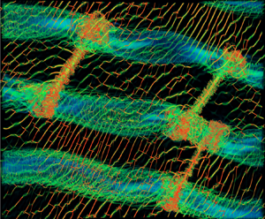
As discussed above, PMCs have provided valuable insights into larger- and smaller-scale dynamics in the polar summer mesosphere for many years. Recent high-resolution PMC imaging from the ground and aboard the PMC Turbo stratospheric balloon flown in July 2018 have revealed a wide variety of KHI dynamics, including billow core twist waves, secondary CI and KHI, billow interactions leading to apparent tubes and knots and their apparent accelerated breakdown of the initial KH billows. A subset of the KHI tube and knot dynamics observed by PMC Turbo is shown in figure 4.
The KH billows exhibiting tube and knots dynamics seen in PMC backscatter brightness,  $\beta$, by a Rayleigh lidar (a) and by a PMC imager (b,c) aboard the PMC Turbo long-duration balloon experiment on 12 July 2018 (Fritts et al. Reference Fritts2019; PMC profiling and imaging courtesy of B. Kaifler, N. Kaifler, and C. B. Kjellstrand). The $\beta$ (colour scale at top right) in an air parcel is relatively constant over short intervals (a few min) for upward displacements, so is an approximate tracer of advection and provides cross-sections of KH billows as they advect through the lidar beam. The images at bottom extend $\sim$50 km from top to bottom with the upper edge at $\sim$35 $^\circ$ off zenith. The KH billow wavelengths were $\sim$5 km, and appear to decrease at larger off-zenith viewing angles. Black arrows highlight bright regions between billows at a 2 min separation, red dashed ovals highlight a region of misaligned billows undergoing strong tube and knot dynamics, orange arrows show secondary CI, yellow arrows highlight secondary KHI between (bright) and below (dark) the billows at $13{:}32$ UT not seen 2 min earlier and red arrows show tubes present at $13{:}30$ UT that are not apparent 2 min later, likely due to rapid tube and knot evolutions.

Figure 4 at top shows an 8 min interval of lidar profiling of PMC backscatter brightness, which serves as a tracer of air motions over short intervals. This exhibits several bright layers that reveal growing KH billows having depths of  $\sim$1.5 km and advection times of $\sim$1.5 min at a relative velocity of ${\sim }60\,{\rm m}\,{\rm s}^{-1}$. PMC Turbo imaging in figure 4 at bottom shows the more fully developed KHI field over an $\sim$50 km field of view at $\sim$20 km away from the lidar profiling separated by 2 min with advection toward lower right.
The PMC imaging spatial resolution of  ${\sim }60\,{\rm m}$ at bottom in figure 4 contributed primarily by the brighter lower PMC layer at $\sim$82 km seen at top in figure 4 enables identification of the $\sim$5 km KH billows (bright regions show upward motions between billows), apparent emerging vortex tubes, secondary CI and KHI and regions without clear KH billow cores where tube and knot dynamics have apparently already diminished KH billow core coherence and strong brightness variations.
These observations and others reviewed above provide evidence of the widespread occurrence of KHI tube and knot dynamics in the atmosphere and likely in all sheared and stratified geophysical fluids enabling sufficiently small  $Ri$ and large $Re$. They also highlight their apparent importance in accelerating and enhancing the turbulence energetics of, and the energy dissipation accompanying, these KHI dynamics where they arise. Importantly, the observations shown in figures 3 and 4 suggest two primary classes of initial KH billow alignments that drive aggressive tube and knot dynamics and dominate the KHI energetics where they arise.
Idealized representations of these two classes of dynamics are shown in figure 5. That at left approximates the dynamics at the sites labelled A–D in figure 3; that at right approximates the dynamics at the sites labelled E and F in figure 3. In both cases, the primary KH billow cores have spanwise vorticity,  $\zeta _y>0$, consistent with the alignment that will be seen in our DNS results below.
Idealized examples of misaligned KH billows (grey with  $\zeta _y>0$) enabling merging and linking (left and right) and emerging vortex tubes (slanted arrows) labelled $\zeta _-$ and $\zeta _+$ both have $\zeta _y>0$ (labelled with respect to their component vorticity along $x$) driving knot dynamics thereafter. Vortex tubes arise on the intermediate vortex sheets due to differential stretching where the KH billows are misaligned along $y$. Note the 90 $^\circ$ rotation relative to figure 3. The left and right cartoons correspond to the knots and tubes, respectively.

Finally, we expect these dynamics to play key roles in the atmosphere, and in oceans and lakes, given the  $Re$ at which they are expected to occur. For a nominal $Re=Uh/\nu \sim 1000$, somewhat smaller than inferred from figure 3, the smallest KH billow in the stable planetary boundary layer can have $\lambda _h$ as small as ${\sim }1\,{\rm m}$, with the largest $\lambda _h\sim 15\,{\rm km}$ or larger at very high altitudes. Oceans and lakes likely enable even smaller minimum $\lambda _h$ of $\sim$10–20 cm and maximum $\lambda _h\sim 100\,{\rm m}$ or larger.
4. Multi-scale KHI dynamics revealed by DNS
4.1. Emergence of misaligned KH billows and vortex tubes
As noted above, the simulation was specified to have a large domain along the KH billow axes to allow exploration of the dynamics of interacting KH billows, the formation of tubes and knots, their breakdown to turbulence and the implications for KHI energetics, energy dissipation and mixing relative to instabilities at locations exhibiting relatively uniform KH billows. Emerging KH billow scales and phases arising from the weak initial noise fields are shown in figure 6 with  $(x,y)$ cross-sections at $z=0$ of $\zeta$, $\lambda _2$ and $T^\prime /T_0$ spanning 3 $T_b$. Both $\zeta$ and $\lambda _2$ are employed because $\zeta$ displays all vorticity features whereas $\lambda _2$ shows only those vortical structures having rotational character. We also use $\zeta$ to denote $|\zeta |$ for convenience except where subscripted.
The  $(x,y)$ cross-sections of $\zeta$, $\lambda _2$ and $T^\prime /T_0$ at $z=0$ from 0–3 $T_b$. Colour scales for $\zeta$ and $T^\prime /T_0$ are shown in each panel and are saturated for $\zeta$ by $\sim$2 and 3 times at 2 and 3 $T_b$. Here, $\lambda _2$ varies from 0 to the domain maximum at each time. Domain dimensions are in units of the nominal KH wavelength, ${\lambda _h}_0=L$.

The  $\zeta$ fields at the first time shown, at which the maximum $|T^\prime /T_0|=0.003$ (denoted 0 $T_b$), reveal weak, structured, small-scale features that are consistent with local optimal perturbations in sheared flows at early times that typically are oriented at $\sim$45 $^{\circ }$ angles to the large-scale shear (Farrell & Ioannou Reference Farrell and Ioannou1996; Achatz Reference Achatz2005; Fritts et al. Reference Fritts, Wang, Werne, Lund and Wan2009). The initial $\lambda _2$ and $T^\prime /T_0$ fields do not exhibit the same structures because they are larger-scale integrated responses to global optimal perturbations that initiate the finite-amplitude KHI features at later times. These larger-scale responses correspond to the two KH wavelengths anticipated by linear stability theory (e.g. 3 or 4 KH billow $\lambda _h$ along $x$, denoted wavenumbers 3 and 4) for the chosen shear depth $h$, as described above.
The three fields in figure 6 exhibit similar larger-scale responses at 1 $T_b$, but $\zeta$ and $\lambda _2$ still reveal smaller-scale responses from $y/L\sim 1.5\text {--}8.5$. Initially disjoint phases in $x$ (denoted $\phi$) begin to exhibit increasingly uniform $\phi$ variations along $y$ by 1 $T_b$, though maintaining a larger-scale ${\rm d}\phi /{{\rm d}y}>0$ (due to the initial noise in a periodic $y$ domain). All fields show decreasing influences by wavenumber 4 KH billows at this time, but there remain multiple sites at which phases along $y$ are misaligned or discontinuous.
The KH billow phases exhibit increasingly uniform  ${\rm d}\phi /{{\rm d}y}$ at most $y$ by 2 $T_b$. See the third warm-to-cold phase transition in $T^\prime /T_0$ (the red/blue gradient with slowly varying $\phi$ along $y$ in figure 6) at $x/L\sim 1.5\text {--}2.5$, especially over $y/L\sim 0\text {--}4$. Corresponding features in $\zeta$ undulate somewhat, but are continuous along $y$ at this stage. The other KH billow phases seen in $T^\prime /T_0$ and $\zeta$ are locally more uniform as well, but exhibit rapid phase transitions or are discontinuous along $y$ at $z=0$; $\lambda _2$ continues to exhibit a lack of vortex structures at the sites of the strongest phase variations seen in the other fields.
All fields show evidence of narrowing phase transitions by 3 $T_b$ at the sites exhibiting the largest initial, and most persistent, phase variations at earlier times; $\zeta$ has evolved thinner, more intense, boundaries between adjacent KH billows that correspond to the vortex sheets between them along $x$ at $z=0$. The regions exhibiting larger ${\rm d}\phi /{{\rm d}y}$ at 2 $T_b$ are seen to evolve coherent vortices having ${\zeta }_z<0$ with large $\lambda _2$ at their outer edges. The $T^\prime /T_0$ fields also reveal vortices passing through $z=0$ having downward motions (red edges) at their positive $x$ edges that confirm vortex tubes also having $\zeta _x<0$ and $\zeta _y>0$ due to their confinement to the vortex sheets between KH billows.
The KH billow cores also exhibit significant structures at 3 $T_b$ at sites adjacent to the vortex tubes noted above. The most obvious are seen in $\zeta$ and exhibit small-scale vorticity having expected links to the adjacent vortex tubes by analogy with the laboratory observations of emerging knots (see the dashed ovals at bottom and upper left in panels (b) and (c) of figure 3, respectively). Corresponding structures are also seen in $\lambda _2$ and more weakly in $T^\prime /T_0$ (see the kinks in the blue/green transitions). These sites will be seen below to be the major drivers of large-scale tube and knot dynamics.
4.2. Instability and turbulence evolutions of misaligned KH billows
We now explore the dynamics of KH billows that have variable phases along their axes, given the evidence for such dynamics from laboratory and atmospheric studies noted above. Our specific interest is the degree to which these dynamics accelerate KH billow breakdown and increase the impacts of KHI tube and knot dynamics relative to those without such influences. Because  $\zeta$ at later times varies by orders of magnitude, we show cross-sections of these fields with a $\log _{10}\zeta$ colour scale hereafter.
Cross-sections of  $\zeta (x,y)$ at $z=0$ and $\zeta (x,z)$ at $y/L=2$, 3, 4, 5.5 and 8.5 from 3-5 $T_b$ are shown at top and bottom in figure 7, respectively. A subset of the $\zeta (x,y)$ domain including the strongest dynamics is shown in figure 8 from 2.75–4.25 $T_b$. Corresponding $T^\prime /T_0(x,y)$ fields at $z=0$ and $T/T_0(x,z)$ fields at $y/L=2$, 3, 4, 5.5 and 8.5, with the latter extending to 10 $T_b$ to show the relative tendencies for restratification, are shown in figure 9.
The  $\zeta (x,y)$ and $\zeta (x,z)$ fields in (a) and (b), respectively, with those in (b) at $z/L=2$, 3, 4, 5.5 and 8.5 from 3–5 $T_b$ at intervals of 0.5 $T_b$ (left to right). Colour scales (upper right in panel (a) where they begin) are logarithmic and saturated to better reveal the evolving dynamics.

As in figure 7 at top for sub-sections of the  $\zeta (x,y)$ fields from 2.5–4.25 $T_b$ at 0.25 $T_b$ intervals. See text for discussion of the highlighted features. Turbulence onset is considered to accompany the rapid emergence of resolved, but much smaller, vortices. Also see the discussion of figures 14 and 15 below.

As in figure 7 for  $T^\prime /T_0(x,y)$ and $T/T_0(x,z)$ (a–c) showing the advective influences of the KH billows, their secondary CIs and KHIs and the tube and knot dynamics at $z=0$ and $y/L=2$, 3, 4, 5.5 and 8.5, respectively. The $T/T_0(x,z)$ panels are extended to 10 $T_b$ at bottom in order to show the approach to a turbulent mixing layer at the various $y$ at later times. Colour scales (upper right in panel a) are shown where they begin.

Figure 7 provides an overview of the evolution from the onset of KH billow interactions and initial tube formation to widespread turbulence  $\sim$2 $T_b$ later. These dynamics are rapid and strong, yield ‘turbulence onset’ at $\sim$3.25 $T_b$ (i.e. emergence of very small scales that are not resolved in the image cadence shown in figure 8) and require only $\sim$0.75 $T_b$ to achieve peak $\zeta$. Importantly, the strongest turbulence transitions occur in regions of misaligned KH billows driving tube and knot dynamics. Secondary KHI and CI also exhibit stronger and more rapid interactions at these sites. In order of emerging turbulence intensities, the major contributors to KH billow breakdown in these regions are, (i) tube and knot dynamics where KH billows have large ${\rm d}\phi /{{\rm d}y}$ and vortex tubes link adjacent billows, (ii) secondary KHI on vortex sheets distorted by tube and knot dynamics and (iii) secondary KHI and CI interactions also influenced by tube and knot flow distortions.
Intensities of tube and knot dynamics driving strong vortex interactions and the rapid cascade to turbulence are not reflected in the colours of the images in figure 7 because the colour scales are saturated in order to reveal dynamics having intermediate  $\zeta$, and the maxima increase by $\sim$20 times from 3 to 4 $T_b$. The true maxima of the $\zeta$ fields at 3, 3.5, 4, 4.5, 5 and 5.5 $T_b$ are $\sim$0.8, 7.5, 7.7, 7.2, 7.7 and 6.9, but the colour scale remains the same at 3.5 $T_b$ and thereafter in order illustrate the decreasing peak turbulence intensities even as additional secondary KHI and CI continue to form and intensify. The influences of tube and knot dynamics are also revealed in the $\zeta (x,z)$ cross-sections in figure 7(b), where the cross-sections at $y/L=4$ and 5.5 reveal more rapid transitions to billow core turbulence and breakdown thereafter.
To further quantify the evolution seen in figure 7(a), expanded views of the most dynamic  $\zeta (x,y)$ domain from 2.5–4.25 $T_b$ at 0.25 $T_b$ are shown in figure 8. Inspection of these panels reveals the following additional details of features seen in figure 7:
(i) billow core interactions where initial ${\rm d}\phi /{{\rm d}y}$ increases and drives differential rotation and kinking along their axes in time (see the billow cores at $y/L\sim 4.5\text {--}6$ at $2.5\text {--}3T_b$);
(ii) large-scale roll-up of the vorticity sheets into tilted vortex tubes where they arise between misaligned KH billow cores (see white arrows at 2.5–3.25
$T_b$ in figure 8);(iii) interactions of vortex tubes and billow cores initiate knots (see red rectangles at 2.75 and 3
$T_b$ in figure 8;(iv) a systematic intensification of the narrow vorticity sheets between adjacent billows (see pink arrows at 3
$T_b$ in figure 8);(v) small-scale billow pairing at
$y/L\sim 2$ (see orange arrows in figure 8a);(vi) initial turbulent breakdown of vortex tubes and knots (see pink rectangles from 3.25-3.75
$T_b$ in figure 8);(vii) secondary KHI on intensifying vorticity sheets
$\sim$0.75-1$T_b$ after initial vortex tube formation and breakdown of vortex knots (see yellow arrows at 3.5 and 3.75$T_b$ in figure 8);(viii) secondary CI in the outer KH billow cores emerging after initial secondary KHI, and occurring first in regions where KH billows are most distorted (see red arrows at 3.5 and 3.75
$T_b$ and elsewhere at later times in figure 8);(ix) turbulence expansion in and between billow cores in the regions of most intense billow core distortions (see yellow rectangles at 4 and 4.25
$T_b$ in figure 8); and(x) delayed and weaker secondary instabilities and turbulence where tube and knot dynamics do not initiate turbulence transitions (see
$y/L=8.5$ in figure 8).


Of these various dynamics, the most significant in driving rapid transitions to turbulence are the evolutions of misaligned KH billows, their stretching of intermediate vortex sheets that drive nearly orthogonal vortex tubes and subsequent interactions and entwining of the vortex tubes and billow cores forming knots. These dynamics account for the accelerated emergence of intense turbulence compared with the evolutions of relatively undisturbed KH billows (such as at  $y/L\sim 0\text {--}1$ and 8–9 spanning the $y$ domain boundary and at $x$ and $y$ where tubes and knots do not occur). For reference, these billows have depths consistent with the laboratory experiments by Thorpe (Reference Thorpe1973b) for $Ri=0.1$.
At 3.5 $T_b$, turbulence is already strong, but is entirely confined to very small regions within emerging tube and knot dynamics. Secondary KHI in the stratified braids and secondary CI in the billow exteriors exhibit enhanced amplitudes in the vicinity of tube and knot dynamics, but only contribute to turbulence where they are entrained into these dynamics. Coherent, larger-scale tube and knot dynamics yield intense, billow-scale turbulence patches, but no billow breakdown or merging by 4 $T_b$ (see figures 7 and 8). As noted in the overview of figure 7 above, turbulence achieves the maximum local $\zeta$ at these times, but will be seen in Fritts et al. (Reference Fritts, Wang, Thorpe and Lund2022) to achieve the maximum local $\epsilon$ from $\sim$4–6.5 $T_b$, depending on whether or not the tube and knot dynamics were the source. The evolutions, vorticity dynamics, transitions to turbulence and relative importance of these various initial tube and knot dynamics for two specific cases are addressed in much greater detail in our exploration via 3-D volumetric imaging of $\lambda _2$ spanning their transitions from initial laminar flows to fully developed turbulence in § 4.3.
The most turbulent KH billows at  $y/L\sim 3$, 4 and 5.5 exhibiting tube and knot dynamics are first to exhibit loss of coherence and initial breakdown to a sheared mixing layer (see these sites at 4.5 $T_b$ in figure 7). Those at $y/L=5.5$ having the strongest initial tube and knot dynamics are seen in figure 7(b) to undergo turbulent billow breakdown up to $\sim$0.5 $T_b$ faster than at $y/L=3$ and 4 and $\sim$1 $T_b$ faster than the KH billow evolutions that are relatively undisturbed by tube and knot dynamics at the extrema of the $y$ domain. Specifically, the three billow cores at $y/L=8.5$ and one billow core at $y/L=2$, where the tube and knot dynamics had small influences remain laminar at 5.5 $T_b$. Regions exhibiting the strongest initial tube and knot dynamics, $y/L\sim 5.5$, 4 and 3 (in order of decreasing influence), also exhibit the most rapid restratification of the turbulent shear layers at these locations. Also seen at $y/L=2$ is a billow-pairing event where billows exhibit displaced vertical positions along $x$ accompanying large-scale vertical motions induced by the tube and knot dynamics.
A complementary perspective on the dynamics beyond 3 $T_b$ is provided by $T^\prime /T_0(x,y)$ and $T/T_0(x,z)$ fields shown in figure 9 that correspond to the $\zeta$ fields in figure 7. As $T$ is constant following parcel motions in a Boussinesq fluid (apart from thermal diffusion), $T^\prime /T_0$ and $T/T_0$ are close tracers of larger- and smaller-scale motions and mixing accompanying these KHI dynamics to late times; $T^\prime /T_0(x,y)$ and $T/T_0(x,z)$ in figure 9 reveal emerging responses to billow roll-up, core structure, breakdown and re-stratification in the absence and presence of tube and knot dynamics that are not revealed as clearly by $\zeta$ in figure 7.
Specific examples of additional insights provided by the  $T^\prime /T_0(x,y)$ and $T/T_0(x,z)$ fields relative to those provided in figures 7 and 8 include the following:
(i)
$T^\prime /T_0(x,y)$ and $T/T_0(x,z)$ provide much clearer evidence of the vertical displacements, billow entrainment and layering causing static stability variations within the billow cores than seen in $\zeta$;(ii)
$T^\prime /T_0(x,y)$ reveal the inferred $\zeta _-$ orientations of secondary KHI between adjacent billows at $z=0$, as for the initial vortex tubes noted above;(iii)
$T^\prime /T_0(x,y)$ and $T/T_0(x,z)$ reveal the scales and character of secondary CI within the billow cores, and regions and extents of mixing events, none of which are apparent in the $\zeta$ fields; and(iv) mean
$T^\prime /T_0(x,y)$ along $x$ at $z=0$ varying in $y$ seen in figure 9 revealing large-scale induced flows extending to late times.


The more significant implications of our discussion of figures 7 and 9 are that the tube and knot dynamics, where they arise, have major influences on the character, intensities and time scales of turbulence transitions relative to those occurring in their absence. These dynamics also suggest more widespread influences in adjacent regions not exhibiting initial tube and knot dynamics due to induced larger-scale motions along  $x$,
$x$,  $y$ and $z$.
$z$.
4.3. Tube and knot dynamics revealed by 3-D visualization
The fields displayed in figures 6–9 reveal several examples of the tube and knot initiation represented in the cartoons in figure 5, approximating sites A−D and E−F, respectively, in figure 3. These are highlighted in figure 10, where Region 1 shows the primary region of initial billow misalignments and Region 2 shows adjacent billows exhibiting weaker phase variations. The early stages in the evolution of the vortex dynamics in Region 1 are shown for reference in figure 11. As the billow cores intensify (blue sheets and arrows in figure 11), they extend along  $y$. Where these billow ‘ends’ are misaligned in $x$ at adjacent $y$, they cause differential stretching of the intermediate (weaker and unseen) vortex sheet along $x$ and $z$ yielding vortex tube formation exhibiting downward and rearward (upward and forward) advection toward smaller (larger) $x$ and $z$ and vortex tube intensification having $\zeta _\pm$ (denoting $\zeta _+$ and $\zeta _-$, respectively, see figure 5) for the KH billow end at larger (smaller) $x$ and $y$ given by
 \begin{equation} \frac{\partial \zeta_\pm}{\partial t}\simeq\zeta_\pm\frac{\partial \zeta_\pm}{\partial r_\pm}\end{equation}
for  $r_\pm$ the distance along $\zeta _\pm$.
As in figure 8 for  $y/L=2.5\text {--}6.5$ at 3.5 $T_b$. Four regions in which 3-D visualization of tube and knot dynamics are presented below are shown with yellow, pink, white, and red rectangles labelled Regions 1, 2, 3 and 4, respectively.

Three-dimensional imaging of  $\lambda _2$ in the yellow sub-domain in figure 10 (Region 1) and extending over $|z/L|\le 0.2$ from the emergence of misaligned KH billow cores to strong interactions among the billow cores and vortex tubes leading to knots. Times are shown in each panel. Peak vorticity increases slowly at early stages, but increases by $\sim$12 times from 3 to 3.5 $T_b$. The more intense features at each time represent <0.1 % of the displayed volume. The colour scales vary from red/orange/yellow/green/blue from large to small negative $\lambda _2$ at each time. The $\lambda _2$ colour and opacity scales also vary between successive images in this and subsequent figures in order to span the range of features and scales appropriate for each local region and evolution.

Vortex tubes having  $\zeta _+$ are shown with the green arrows at 2.5 $T_b$. Those having $\zeta _-$ have roughly orthogonal orientations and attach to the trailing KH billow end below and rearward (yellow arrows at 2.5 $T_b$). The initial tube and knot features (white arrows at 2.75 $T_b$) exhibit roughly orthogonal vortices in close proximity that yield intense stretching (dashed arrows at 3 $T_b$), or axial compression, of both vortices and intensifying interactions, enstrophy cascades and enhanced energy dissipation thereafter. Successive images in figure 11 show further intensification of the initial vortex tubes and knots, both knot and initial KH billow core breakup due to twist wave generation, and the emergence of secondary KHI and tube and knot dynamics on the intensified and distorted vortex sheets in close proximity to the initial tube and knot dynamics. Also see the more detailed discussions of these tube and knot dynamics in §§ 4.3.1–4.3.3 and 4.4.)
The results of these dynamics are the mutual intensification of the kinked billow cores and orthogonal vortex tubes yielding wrapping of these features at the initial billow core ‘ends’ and formation of features referred to as knots in the early laboratory shear-flow studies by Thorpe (Reference Thorpe1985, Reference Thorpe1987, see figure 3). These knots entwine the intensifying, orthogonal vortex tubes, and drive them increasingly into closer proximity. This results in dramatic accelerations of these interactions and induced differential axial and radial advection of the vortex cores that result in excitation of Kelvin twist waves at larger scales initially and successively smaller scales rapidly thereafter (see figure 11 at 3.25 and 3.5 $T_b$). The latter panels reveal the evolution from a laminar initial flow to intense smaller-scale interactions within 0.5 $T_b$ measured with respect to the large initial $N$ at $z=0$. These dynamics are explored in detail below for (i) the single vortex tube linking two adjacent KH billow cores in the pink sub-domain (Region 2) and (ii) the two vortex tubes linking to a single KH billow core in the white sub-domain (Region 3) in figure 10.
4.3.1. Tube and knot dynamics of one tube linking two KH billows
Tube and knot dynamics accompanying the evolution of the single vortex tube linking adjacent KH billow cores in Region 2 is shown with 3-D imaging viewed from above in figure 12 and from above, more positive  $x$, and more negative $y$ in figure 13. These figures employ colour and opacity scales that vary in time as $\lambda _2$ magnitudes increase and between the two views at common times. This is because no colour and opacity scales allow inter-comparisons spanning the weak initial magnitudes, the very large range of magnitudes accompanying strong turbulence at later times, and only relative $\lambda _2$ magnitudes are relevant at each stage of the evolution. Supplementary Movie 1 and Supplementary Movie 2 provide animations of these figures at https://doi.org/10.1017/jfm.2021.1085.


As in figure 12 from 3.1–4 $T_b$ viewed from larger $x$, smaller $y$ and positive $z$.
$z$.

The  $\lambda _2$ fields at 2.75 $T_b$ in figures 12 and 13 reveal that both KH billow cores aligned approximately along $y$ and the inclined vortex tube exhibit differential rotation along their axes due to axial stretching and compression where they are in close proximity. The vortex tube rotation, in particular, has increased dramatically relative to the billow cores by this time due to stretching of the intermediate vortex sheet described above and their increasing proximity thereafter. These initial large-scale dynamics drive an accelerating cascade of vortex interactions leading to intense, fully developed turbulence within 1 $T_b$. Specific features of the subsequent dynamics include the following:
(i) the vortex tube is stretched and intensified where it is advected over and under the billow cores forming knots as the billow amplitudes increase (see sites labelled a from 2.75–3.1
$T_b$ in figures 12 and 13);(ii) vortex and billow core interactions in the knot regions begin to drive smaller-scale perturbations that manifest as twist waves at 3.2 and 3.3
$T_b$ (sites b) that are much stronger than the larger-scale twist waves emerging in the billow cores in figure 11; they also induce vortex tube perturbations that intensify in time (site c);(iii) seen emerging in the knot regions by 3.3
$T_b$ are smaller-scale vortex features in and external to the knots that had their roots in the initial distorted vortex sheet that is intensified due to stretching by the evolving knots (sites d from 3.4–3.6$T_b$);(iv) a sheath of small-scale vortices is seen wrapping around the vortex tubes that are distinct from the induced twist waves and result from intensification of small-scale KHI on the evolving and entraining vortex sheet beginning at 3.3
$T_b$ (site e) noted in the discussion of figure 11, but seen more clearly here;(v) larger-scale twist waves arise due to unravelling of perturbed vortex tube ends that propagate inward toward the centre of the vortex tube extending from
$\sim$3.3–3.6$T_b$ (sites d at larger scales);(vi) the initial vortex tube weakens and begins to disappear due to fragmentation accompanying larger-scale mode-2 twist wave excitation by
$\sim$3.5$T_b$;(vii) secondary KHI emerge primarily along, but external to, the initial KH billow cores by 3.5
$T_b$ (sites f);(viii) weak secondary CI also arise having initial streamwise and vertical alignments in the billow exteriors by 3.5
$T_b$ (sites g);(ix) the knot regions remain the sites of most intense turbulence and exhibit rapid cascades of fully resolved, smaller-scale vortex dynamics that yield a broad turbulence inertial range with
$\eta < L$/1000 by 4$T_b$;(x) the turbulence fields exhibit discernible vortex structures extending down to scales of <0.01
$L$ (thus $\sim$6$\Delta x$ at these times); and(xi) small-scale secondary KHI exhibit interactions yielding secondary tube and knot dynamics in close proximity to the larger-scale knots by 3.6–3.8
$T_b$ (sites h) and are explored in greater detail below.


Our discussion above reveals both a significant acceleration of KHI breakdown to turbulence due to tube and knot dynamics and apparent major increases in the scales and intensities of the dominant turbulence events in these regions relative to KH billows not undergoing tube and knot dynamics. A second region of tube and knot dynamics having different character is examined below to assess the universality of these dynamics within the larger-scale multiple KH billow environment.
4.3.2. Tube and knot dynamics of two tubes linking to one KH billow
Tube and knot dynamics arising where two tubes link to one KH billow core are shown in figures 14 and 15 employing similar viewing perspectives to those in § 4.3.1, but for Region 3 shown with the white rectangle in figure 10. The 3-D fields in figures 14 and 15 reveal that these dynamics emerge at very nearly the same time and span roughly the same interval as those described in § 4.3.1. They exhibit similar tube and knot evolutions and influences on the initial larger-scale vortex features in many respects, but there are also quantitative differences having implications for turbulence evolutions and intensities. For ease of comparisons of the two types of vortex dynamics, we employ the same feature labelling as in § 4.3.1. Supplementary Movie 3 and Supplementary Movie 4 provide animations of these figures.
As in figure 12 for  $\lambda _2$ in Region 3 highlighted by the white rectangle in figure 10 viewed from above and spanning times from 2.75–4 $T_b$ (see axes at 2.75 $T_b$). Note the more rapid excitation of larger-scale twist waves that drive faster breakdown of the billow core and vortex tubes relative to those seen in Region 2 in figures 12 and 13.


Specific features of these dynamics, and differences from those in Region 2 discussed in § 4.3.1, include the following:
(i) vortex tubes at smaller (larger)
$x$ (sites c) wrap over (under) the KH billow core because of their formation and intensification on the vortex sheet between adjacent billows (sites a in figures 14 and 15 which closely resemble sites a in Region 2);(ii) the tubes and billow core exhibit mutual stretching (compression) along their axes due to differential advection by each other (sites a and b at 2.75 and 3
$T_b$), but stretching by closely spaced tubes acts more strongly on the KH billow core in Region 3;(iii) sheaths of smaller-scale vortices are seen wrapping around both vortex cores due to entraining of the initial vortex sheet having embedded and enhanced small-scale secondary KHI, as in Region 2 (see sites c from 3–3.7
$T_b$);(iv) KH billow core stretching between the vortex tubes in Region 3 increases its rotation and enables
$\lambda _2$ revealing the emergence of billow core twist waves at 3.2 and 3.5$T_b$ not seen in Region 2;(v) large-scale twist wave propagation along the vortex tubes away from their source regions (sites b and d) toward negative (positive)
$x$ along the tube at smaller (larger) $y$, that are much more dramatic than seen in Region 2;(vi) smaller-scale twist waves also arise on larger-scale twist waves where they are perturbed by other vortex features (sites d at
$\sim$3.5$T_b$ and beyond);(vii) as in Region 2, secondary KHI form and initiate interactions and secondary tube and knot dynamics on the vortex sheet deformed and intensified by the larger-scale tube and knot dynamics (sites f and g); and
(viii) as in Region 2, the knots in Region 3 remain the sites of the most intense turbulence, achieve a broad turbulence inertial range with
$\eta < 3L/1000$ and exhibit clear vortex structures extending down to scales of <0.01$L$ by 4$T_b$.


In summary, the tube and knot dynamics in Region 3 exhibit several clear differences relative to those occurring in Region 2. The most significant arise from the stretching by two vortex tubes of the common KH billow core, which enables much stronger interactions among larger-scale vortices in close proximity having roughly orthogonal alignments. In Region 2, in contrast, the vortex tube ‘ends’ interact with relatively weaker orthogonal billow cores. These differences clearly account for the very different twist wave formation dynamics seen in these two regions, and the larger energy dissipation rates in Region 3 as described in the companion paper by Fritts et al. (Reference Fritts, Wang, Thorpe and Lund2022).
4.3.3. Secondary KHI and CI evolutions influenced by adjacent tube and knot dynamics
We noted the tendency for enhanced secondary KHI and CI in close proximity to emerging tube and knot dynamics in the discussions of figures 11–15 in Regions 1, 2 and 3. To explore these dynamics in greater detail, figure 16 provides an expanded time series of figure 12(f–h) from 3.6 and 4 $T_b$ using optimized $\lambda _2$ and opacity scales in the Region 4 red rectangle in figure 10. These show the region between the two initial KH billows at smaller $x$ and $y$ relative to the large initial vortex tube at upper right linking the KH billows in Region 2. For reference, these images span only $\sim$5 % of the full horizontal domain seen at top in figure 7.
As in figure 12 for  $\lambda _2$ in the lower left portion of Region 2 shown with the red rectangle in figure 10 (Region 4) viewed from above and spanning the interval from 3.6–4 $T_b$. It includes the right portion of the large-scale KH billow that is relatively uniform along $y$ at left and the left edge of the KH billow at right having ${\rm d}\phi /{{\rm d}y}>0$.

As discussed in § 4.3.1, the upper left and lower right portions of this region exhibit intensifying to strongly interacting secondary KHI (sites a) where the vortex sheet is enhanced and deformed by the KH billows in close proximity. Weaker secondary KHI emerge on the less enhanced vortex sheet between adjacent KH billows (site b) at 3.6 $T_b$. These vortex evolutions progress rapidly thereafter, and we employ different site labels with advancing subscripts to track the evolutions of individual features in time. Features labelled c–i in the panel at 3.7 $T_b$ evolving to features labelled ${\rm c}_3-{\rm i}_3$ in the panel at 4 $T_b$ reveal often significant evolutions of these small-scale dynamics over only 0.3 $T_b$.
Key features of the secondary KHI, vortex tubes and secondary CI evolutions in this region include the following:
(i) initial secondary KHI have primary
$\zeta _-$ alignments opposite that of the initial KH billow cores driving the large-scale tube and knot dynamics (see figures 11 and 12 at 2.75$T_b$ and sites a);(ii) secondary CI in the outer billows are roughly orthogonal to the billow cores, see the blue/green features at sites b, i and j outside the tube and knot dynamics where the KH billows are more nearly aligned along
$y$, but they fail to compete with the secondary tube and knot dynamics in these regions;(iii) the secondary KHI and vortex tubes exhibit variations in their orientations along their axes at earlier times due to weak perturbations of the deforming initial vortex sheet (see sites c, d and e at 3.7
$T_b$ and figure 11 at 3.5$T_b$);(iv) the secondary KHI having
$\zeta _-$ are more nearly continuous along their axes, whereas the vortex tubes having $\zeta _+$ alignments instead terminate at the orthogonal $\zeta _-$ tubes, as also seen in the initial large-scale dynamics, but rotated $\sim$90$^\circ$ clockwise;(v) secondary KHI and vortex tubes with
$\zeta _-$ and $\zeta _+$ alignments intensify due to vortex sheet stretching, lead to an extended ‘web’ of nearly orthogonal secondary billow cores and vortex tubes, and rapid evolutions of small-scale tube and knot dynamics mirroring the initial large-scale tube and knot alignments, but at scales $\sim$10 times smaller, and thus strongly constrained by a very small $Re$ (see sites $c_i-h_i$ for $i=1\text{--}3$ from 3.8−4$T_b$); and(vi) emerging complexity in the outer KH billows not undergoing tube and knot dynamics where secondary CI and KHI interact and lead to mutual stretching and deformation, but at very small scales that exhibit relatively small intensities due to their very small
$Re$ (see sites i$_i$ and j$_i$ from 3.7–4$T_b$).


These results reveal that KHI tube and knot dynamics are widespread across scales within individual events, and that they arise readily wherever initial vortex sheets intensify and form KHI for sufficiently small local  $Ri$, even when their scales and intensities are constrained by low local $Re$. More importantly, secondary KHI tube and knot dynamics contribute weakly to turbulence intensities where these smaller KHI, by themselves, would fail to yield turbulence. This suggests that such dynamics may contribute to turbulence and mixing where traditional KHI is not expected to do so.
4.4. Secondary KHI and CI evolutions without strong tube and knot influences
As noted above, the absence of significant KHI  ${\rm d}\phi /{{\rm d}y}$ at small and large $y$ enables KH billow breakdown via secondary KHI and CI largely without influences of large-scale tube and knot dynamics. These secondary instabilities arise from the same initial noise seed, but where it does not induce significant KHI phase variations leading to large-scale tube and knot dynamics. The primary KHI and secondary instability dynamics centred at $y/L=8.5$ are shown for the two central billow cores along $x$ with 3-D imaging of $\lambda _2$ viewed from above and from larger $x$, smaller $y$ and positive $z$, respectively, at left and right in figure 17 at the later times discussed above. The later emergence of these secondary instabilities, and their relatively slow progressions to initial turbulence compared with the tube and knot dynamics discussed in § 4.3, are our focus here. Supplementary Movie 5 and Supplementary Movie 6 provide animations of this figure.
As in figure 12 for  $\lambda _2$ from $x/L=0.5\text {--}2.5$ and $y/L=8\text {--}9$ (a,c,e) showing emergence of initial secondary instabilities yielding initial transitions to turbulence. The same 3-D fields are shown at right viewed from larger $x$, smaller $y$, and positive $z$ (b,d,f). See text for details.

The 3-D imaging of  $\lambda _2(x,y)$ viewed from above at left in figure 17 from 3.5–3.9 $T_b$ exhibits two KH billows having coherent cores with small ${\rm d}\phi /{{\rm d}y}$ and ${\rm d}^2\phi /{{\rm d}y}^2<0$ and $\sim$0 at smaller and larger $x$ at 3.5 $T_b$, and rapid decreases in billow core $\lambda _2$ relative to secondary KHI and CI thereafter. The imaging also reveals the emergence of secondary KHI and CI that drive secondary tube and knot events that dominate the weak turbulence transitions at later times. Specific features seen in figure 17 include the following:
(i) evidence of initial weak secondary KHI and CI arises in the vortex sheets and the KH billow interiors (see sites a and b, respectively, at 3.5
$T_b$);(ii) increasing secondary KHI amplitudes exhibit distinct
$\zeta _-$ and $\zeta _+$ and undergo initial interactions at 3.7$T_b$ having the same forms seen in regions adjacent to the larger-scale tube and knot dynamics (see sites c, and compare with figure 16 at earlier times);(iii) small-scale secondary CI in the KH billow exteriors intensify dramatically by 3.7
$T_b$, comprise counter-rotating vortices that wrap around the billow cores and induce intensifying vortex sheets where vortex pairs stretch and distort adjacent, small-scale vortex sheets having primarily $\zeta _y$ (see sites d and e);(iv) interactions among secondary KHI and vortex tubes on the vortex sheets between and around the KH billows induce smaller-scale knots, twist wave generation, and initial small-scale twist waves driving turbulence (see sites f in figure 17 at 3.9
$T_b$);(v) interactions between secondary KHI and CI at the outer edges of the KH billows cause intensification of
$\lambda _2$ where CI vortices cross secondary KHI on entraining vortex sheets (see site g and others that are similar at 3.9$T_b$); and(vi) regions where interacting secondary KHI and CI induce further tertiary interactions comprising largely orthogonal vortices in close proximity that are very small-scale versions (scales of
$\sim$0.03$L$) of primary and secondary tube and knot interactions discussed above, but now at dramatically smaller $Re$ (see sites h).


This discussion of the interactions and dynamics of secondary instabilities of individual KH billows reveals features of these interactions that could not be inferred in the analyses of the larger-scale tube and knot dynamics in § 4.3. This is due to the inability of these larger-scale, more intense dynamics to also reveal the much weaker dynamics at much smaller scales, despite the expectation that they will also occur. These various instability events are compared in spectral assessments spanning their evolutions in § 5. Their potential implications for enhanced turbulence and mixing are discussed in § 6.
5. Velocity variance and enstrophy spectra for tube and knot dynamics and secondary KHI and CI of individual KH billows
Results presented above reveal earlier and more energetic transitions to turbulence accompanying tube and knot dynamics relative to regions exhibiting delayed or no obvious tube and knot dynamics. Figures 11–15 show the tube and knot dynamics to emerge most energetically at  $y/L\sim 3\text {--}5.5$ from $\sim$3.3–3.5 $T_b$. Figures 7, 8, 9 and 17 reveal turbulence transitions to occur $\sim$0.5 $T_b$ later in the absence of tube and knot dynamics. The $\lambda _2$ images shown above for the various $y/L$ reveal the cascade to smaller scales into and within the turbulence inertial range, but they do not allow comparisons of the varying intensities of these events in time. To do so, velocity variance and enstrophy spectra averaged over $\Delta {y}=0.2L$ and $\Delta {z}=0.6L$ about $z=0$ are shown for the various $y/L$ from 3–10 $T_b$ in figure 18. Corresponding variance-content spectra are shown in figure 19. The variance spectra confirm very different evolutions for the regions exhibiting, and not exhibiting, initial tube and knot dynamics. The former centred at $y/L=3$, 4 and 5.5 in the middle three rows of figure 18 show peak inertial-range amplitudes attained from 4-6 $T_b$ and decreasing, but variable, amplitudes in time and among components thereafter. Spectral peaks seen at the primary KH billow wavenumber, $k=2{\rm \pi} /L$, and its harmonics persist beyond $\sim$5 $T_b$ and likely account for local flow orientations contributing to the variable inertial-range amplitudes at these times. The $\langle w'^2\rangle$ amplitudes are also significantly suppressed at smaller $k$ at later times due to KH billow breakdown and restratification beginning $\sim$4.5-5 $T_b$ at $y/L=3\text {--}5.5$ (see figure 7).
Component variance (panels a–c) and enstrophy spectra (panel d) from 3–10 $T_b$ at $y/L=2$, 3, 4, 5.5 and 8.5 (bottom to top). Dashed lines show a $-5/3$ slope.

Velocity variance and enstrophy spectra (a,c,e,g,i and b,d,f,h,j) in variance-content form revealing the different scales of large velocity variance and enstrophy more clearly.

Variance spectra at  $y/L=8.5$ differ from those at the sites of tube and knot dynamics in several ways. The magnitude of $\langle w'^2\rangle$ increases rapidly at early times, coincident with those at $y/L=3\text {--}5.5$, but does not attain the same amplitude, nor the more extended inertial range seen at those sites. In contrast, $\langle u'^2\rangle$ and $\langle v'^2\rangle$ do not increase as quickly, but retain larger amplitudes to later times due to later primary KH billow breakdown at $y/L=8.5$ seen in figure 7. The spectral evolution at $y/L=2$ exhibits features similar to both the sites of tube and knot dynamics and at $y/L=8.5$ without them, due to its closer proximity to the former at $y/L=3$. These include more rapid inertial-range amplitude increases, later amplitude maxima and $\langle w'^2\rangle$ suppression less (greater) than at $y/L=3\text {--}5.5$ (8.5). Enstrophy spectra in figure 18(d) are surrogates for energy dissipation at smaller scales. They emphasize the differing rates at which the emerging turbulence at different $y/L$ attain their strongest responses. As expected from the discussion of figures 14 and 15, the most rapid transitions occur at $y/L=5.5$ and 4, followed in order by $y/L=3$, 2 and 8.5 due to the decreasing influences of nearby tube and knot dynamics. The enstrophy spectral slopes are not +1/3 because these are 1-D, rather than 3-D, spectra.
Additional insights into the various evolutions are provided by variance-content spectra in figure 19. These show the same spectra as figure 18, but display a number of key features more clearly. Key features and implications of these spectra include the following:
(i) the KH billows and their harmonics dominate the component variances at all sites to
$\sim$5$T_b$ or thereafter, except where the initial KH billows exhibit pairing at $y/L=2$;(ii) the tube and knot dynamics at
$y/L=5.5$ account for the most rapid initial KH billow breakdown by $\sim$6$T_b$, followed in order by $y/L=4$, 3, 2 (despite pairing) and 8.5 (last to exhibit turbulent billow cores);(iii) peak enstrophy occurs for all
$y/L$ at $k\sim 200\text {--}400{\rm \pi} /3L$;(iv) tube and knot dynamics at
$y/L=5.5$ exhibit the earliest peak enstrophy, followed in succession by $y/L=4$, 3, 2 and 8.5; and(v) peak enstrophy is larger at later times at
$y/L=2$ and 8.5 than at the sites of earlier tube and knot dynamics.


6. Relations to previous studies of KHI and turbulence transitions
Results presented above show KHI evolutions exhibiting tube and knot dynamics to differ dramatically from those of KH billows that are more uniform along their axes. This finding is not surprising, given the multiple, early laboratory observations of tube and knot dynamics revealing its acceleration of turbulence transitions (Thorpe Reference Thorpe1973b, Reference Thorpe1985, Reference Thorpe1987; Caulfield et al. Reference Caulfield, Yoshida and Peltier1996). Additional motivations for studies of KHI tube and knot dynamics based on observations of limited KH billow coherence lengths and apparent KHI exhibiting misaligned billows were provided by Thorpe (Reference Thorpe2002). But no modelling studies arose, perhaps due to the computational challenges of modelling multiple KH billows in a large domain at very high resolution. In contrast, there have been extensive theoretical and modelling studies addressing the ‘zoo’ of secondary instabilities of individual KH billows arising for varying  $Ri$,
$Ri$,  $Re$,
$Re$,  $Pr$ and multiple mean state configurations (Mashayek & Peltier Reference Mashayek and Peltier2012). These instabilities are all specifically enabled by the chosen $Ri$,
$Ri$,  $Re$ and noise seeds in our multi-scale DNS, but they appear not to compete effectively with the tube and knot dynamics largely accounting for KH billow breakdown where they arise.
Further motivations for modelling addressing KHI tube and knot dynamics were provided by more recent observations arising on large spatial scales at  $\sim$82–90 km altitudes in the atmosphere; see (Hecht et al. Reference Hecht, Fritts, Gelinas, Rudy, Walterscheid and Liu2021) and figure 4. The first motivated the study by Fritts et al. (Reference Fritts, Wieland, Lund, Thorpe and Hecht2021) of KHI tube and knot dynamics performed using a deep, compressible model addressing these dynamics for KH billow $\lambda _h\sim 7\text{--}10\,{\rm km}$. However, that modelling did not employ the high spatial resolution required for a DNS description enabling a quantitative assessment of tube and knot dynamics initiation, their energetics nor their progression to inertial-range turbulence. It also prescribed initial misaligned KH billow cores in order to assure vortex tube formation where KH $\lambda _h$ differed at smaller and larger $y$. This imposed a merging of two billow cores with one at several sites, as seen in the regions labelled ‘A’ and ‘D’ in figure 3(a,b). The resulting dynamics included (i) misaligned KH billow cores causing stretching of the intermediate vortex sheets leading to roughly orthogonal vortex tubes, (ii) vortex tubes that wrapped around each other where they attached to a common billow core and (iii) entwining and intensifying interactions spawning twist waves and entrainment of the secondary CI and KHI. However, the lack of DNS resolution precluded a quantitative representation of the evolution and cascade to smaller scales subsequent to the initial tube interactions.
Previous modelling studies of unstratified and stratified mixing layers revealed the emergence of KH billow misalignments along their axes and/or quasi-streamwise vortex tubes accompanying larger-scale KH billow evolutions. Earlier LES studies by Comte et al. (Reference Comte, Silvestrini and Begou1998) revealed KH billow misalignments along their axes that induced vortex tubes closely resembling those described above, but were unable to describe the evolution to smaller spatial scales. A higher-resolution LES study by Balaras et al. (Reference Balaras, Piomelli and Wallace2001) showed a diversity of responses exhibiting KH billow misalignments along their axes, vortex tubes linking adjacent KH billows and multiple apparent tube and knot events, but at resolutions unable to describe their cascades to smaller scales, suggesting similar tube and knot dynamics with and without stratification. Jimenez & Wray (Reference Jimenez and Wray1998) and Watanabe et al. (Reference Watanabe, Riley, Nagata, Matsuda and Onishi2019) identified streamwise vortices emerging at later stages in KHI mixing layer evolutions. A further DNS study by Watanabe & Nagata (Reference Watanabe and Nagata2021) captured similar dynamics, noting only that it accelerated the transition to turbulence. Lasheras & Choi (Reference Lasheras and Choi1988) employed a splitter plate inducing periodic vertical displacements across the shear flow that modulated and linked successive KH billows via counter-rotating streamwise vortices. These vortices exhibited features resembling those identified here, but their paired structures are quite different from the vortex tubes arising in our DNS.
Implications of our study, and that by Fritts et al. (Reference Fritts, Wang, Thorpe and Lund2022), are that KHI tube and knot dynamics result in more rapid and vigorous transitions to turbulence than occur in their absence. The choices to enable secondary KHI in these studies suggest that increasing  $Re$ will not enable these dynamics to compete with tube and knot dynamics. Conversely, these results suggest that tube and knot enhancements of secondary KHI may enable secondary KHI to arise in tube and knot regions for smaller $Re$ that preclude them elsewhere. Lastly, because tube and knot dynamics arise at spatial scales much larger than secondary KHI, we expect them to be robust and lead to turbulence for smaller $Re$ and/or larger $Ri$ that would preclude turbulence and mixing in their absence.
The helical vortex structures seen to arise at early stages of the interactions of vortex tubes and billow cores driving knot formation, and the successively smaller helical vortices arising due to subsequent interactions of larger-scale features where they emerge in close proximity, are apparent finite-amplitude manifestations of vortical waves, or ‘twist waves’, first described by Kelvin (Reference Kelvin1880). Our results reveal twist waves to arise where initial, roughly orthogonal interacting vortex tubes and KH billow cores induce perturbations along and across each other via differential axial stretching and compression. These mutual interactions are especially strong accompanying vortex tube or KH billow core ‘ends’ that drive initial vortex knots. The primary responses in such regions are unravelling and fragmentation of the initial vortices driving a cascade of similar dynamics at successively smaller scales.
Similar vortex dynamics arose in the initial, relatively high-resolution simulation of breaking GWs by Andreassen et al. (Reference Andreassen, Hvidsten, Fritts and Arendt1998). That study revealed such vortex alignments to emerge where roll-up of spanwise-localized, intensifying shear layers yielded successive, small-scale KHI leading to vortex rings in close proximity. These yielded roughly orthogonal vortex interactions that excited mode 1 and 2 twist waves (having axial wavenumbers 1 and 2, respectively) that (i) propagated in opposite directions from their source regions due to the radial and axial advection of the vortex tube induced by the twist wave tube displacements and (ii) increased in amplitude with sufficient forcing that led to vortex tube unravelling, fragmentation and a cascade to smaller scales, as described above; see Arendt et al. (Reference Arendt, Fritts and Andreassen1997) and Fritts et al. (Reference Fritts, Arendt and Andreassen1998). A parallel analysis by Arendt & Fritts (Reference Arendt and Fritts1997) revealed that an idealized vortex tube is unstable to both external shear and strain. Hence, the generation and evolution of twist waves appear to be central to the transitions from laminar to turbulent flows accompanying the various local tube and knot dynamics described above, and we expect that they also account for the dynamics driving the major identified sources of turbulence in the atmosphere and oceans. Given the pervasive occurrence of significant helicity in various modelled turbulent flows, we suggest that ‘twist waves’, for which there are evolution equations and a dispersion relation at small amplitudes, are a natural physical description of such helical features observed in more general turbulence flows.
Importantly, our choice to address KHI for  $Pr=1$ enabled the most efficient DNS of these dynamics for our chosen $Re$ and $Ri$, but it does not enable exploration of the potential for subcritical stable (supercritical unstable) responses anticipated for $Pr>1$ (<1) at $Ri\sim 0.25$ and larger, nor the influences at smaller $Ri$. Earlier theoretical and modelling studies revealed $Pr$ influences on KHI stability (Klaassen & Peltier Reference Klaassen and Peltier1985; Salehipour, Peltier & Mashayek Reference Salehipour, Peltier and Mashayek2015; Rahmani, Seymour & Lawrence Reference Rahmani, Seymour and Lawrence2016) and nonlinear, viscous departures from expectations based on linear inviscid theory (Brown, Rosen & Maslowe Reference Brown, Rosen and Maslowe1981; Churilov & Shukhman Reference Churilov and Shukhman1987; Lott & Teitelbaum Reference Lott and Teitelbaum1992; Brucker & Sarkar Reference Brucker and Sarkar2007); see the recent discussion by Parker, Caulfield & Kerswell (Reference Parker, Caulfield and Kerswell2021). The KHI tube and knot dynamics described here may play a key role in turbulence transitions for $Pr\ne$1 that will be addressed in subsequent DNS modelling applications for various $Re$,
$Re$,  $Ri$ and $Pr$.
$Pr$.
7. Summary and conclusions
Our simulation results demonstrate the significance of, and transitions to turbulence accompanying, KHI tube and knot dynamics arising from interactions among KH billows which have variable phases along their axes. Their significance derives from (i) wide-spread occurrence of KHI throughout the atmosphere, in the oceans and likely in other geophysical fluids at high  $Re$, (ii) relatively small KHI coherence lengths suggesting frequent KHI misalignments and interactions and (iii) dramatically stronger and more rapid vortex dynamics and turbulence generation accompanying tube and knot dynamics compared with secondary instabilities of individual KH billows. These aspects of KHI tube and knot dynamics suggest that they may play more significant roles in energy dissipation, mixing and transport in the atmosphere, oceans and other geophysical fluids than previously believed, as described by Fritts et al. (Reference Fritts, Wieland, Lund, Thorpe and Hecht2021) and in other studies now underway.
Tube and knot dynamics arising due to misaligned KH billows can take various forms, as revealed in early laboratory studies by Thorpe (Reference Thorpe1973a, Reference Thorpe1987, Reference Thorpe2002) and others. We explored two examples of these dynamics in detail, including (i) a single vortex tube linking adjacent KH billow cores and (ii) two vortex tubes attaching to a single KH billow core in close proximity. A third example (seen in the laboratory and the atmosphere) expected to be at least as significant is the linking of three KH billows to two billows (or of two KH billows linking to one) where their cores are misaligned (as seen in figure 3 at sites labelled A−D), but such a case did not arise here.
The tube and knot dynamics that did arise demonstrated transitions to turbulence that occurred  $\sim$0.5 $T_b$ earlier and yielded accelerated KH billow breakdown to turbulence by $\sim$1.5 $T_b$ or greater, compared with regions largely unaffected by tube and knots dynamics. In each case, local vortex tube and KH billow core interactions arose where a vortex tube (or tubes) forming due to axial stretching of the vortex sheet between adjacent KH billows wrapped over or under adjacent billows and began to attach at the outer edges of the billow cores. These evolutions drove emerging, roughly orthogonal entwining, co-rotation and local interactions that yielded intense stretching and compression of each element, and spawning of twist waves that propagated along each component and contributed to its unravelling and fragmentation. Successive interactions among the emerging vortex structures, on the intensifying vortex sheets between interacting KH billows and elsewhere, led to similar dynamics at spatial scales down to $\sim$0.01 $L$ driving rapid, and accelerating, cascades extending well into the turbulence viscous range (with a Nyquist scale $\sim$0.003 $L$).
$L$).
We expect similar dynamics to accompany other forms of tube and knot initiation and progression, and that such dynamics may also enable strong turbulence and mixing to occur at smaller  $Re$ and/or larger $Ri$ (including $Ri\sim 0.25$ and larger) for which either or both secondary CI and KHI of individual KH billows are not anticipated, based on the above discussion and other initial KHI modelling studies to date. Tube and knot dynamics have not yet been assessed for $Pr \ne 1$, but such will be important in assessing their potential for enhanced turbulence and mixing throughout the atmosphere and oceans.
Supplementary movies
Supplementary movies are available at https://doi.org/10.1017/jfm.2021.1085.
Funding
Research described here was supported under the U.S. Air Force Office of Scientific Research (AFOSR) under grant FA9550-18-1-0009 and the U.S. National Science Foundation (NSF) under grants AGS-1758293, AGS-2032678 and AGS2128443 listed in the U.S. Grant Electronic Management System. We also acknowledge the U.S. Department of Defence High Performance Computing Modernization Program (HPCMP) for significant resources employed for our multiple smaller and larger DNS.
Declaration of interests
The authors report no conflict of interest.


 Open access