BACKGROUND

Historians and social scientists have long noted the role of churches in providing various forms of social and economic support. In the United States, the nineteenth-century Social Gospel movement coincided with an increase in church activity dedicated to addressing poverty, inequality, and education (Cnaan et al. Reference Cnaan, Boddie, Handy, Yancey and Schneider2002). Prior to the advent of federal government welfare and social insurance programs in the 1930s,^{Footnote 8} religious communities had become a leading provider of financial assistance and other aid, such as food and clothing, as well as employment matching services, job and vocational training, and other social services (Gruber and Hungerman Reference Gruber and Hungerman2007; Chen Reference Chen2010). In 1926, for example, churches provided a total of $150 million in charitable spending, according to the U.S. Census of Religious Bodies. In comparison, social and charitable spending by state governments amounted to $23 million, and $37 million by local governments in the same year (Gruber and Hungerman Reference Gruber and Hungerman2007).

Even today, churches play an active role in providing important support to their communities, particularly where formal mechanisms for dealing with economic uncertainty are lacking (Bartkowski and Regis Reference Bartkowski and Regis2003; Hungerman Reference Hungerman2005; McCleary and Barro Reference McCleary and Barro2006; Scheve and Stasavage Reference Scheve and Stasavage2006). One U.S. study by Cnaan et al. (Reference Cnaan, Boddie, Handy, Yancey and Schneider2002) finds that about 75 percent of congregations have some form of financial support mechanism for the poor, while Glaeser and Sacerdote (Reference Glaeser and Sacerdote2008) note that three in five Catholics and three in four Baptists in the U.S. General Social Survey trust their congregation to help them in times of hardship. The sources of such support tend to be the voluntary contributions of other members.^{Footnote 9} This is consistent with club models of religion and subsequent empirical work documenting how religious communities provide local public goods to their members, derived from the religious “investments” of members such as tithing and service-based contributions (Iannaccone Reference Iannaccone1992, Reference Iannaccone1998). To the extent that major religious organizations span networks of individuals and communities with idiosyncratic risk and state realizations, churches thus entail an important source of mutual insurance and consumption smoothing for religious participants (Berman Reference Berman2000; Chen Reference Chen2010; Ager and Ciccone Reference Ager and Ciccone2018).^{Footnote 10}

OIL ABUNDANCE AS A SOURCE OF RISK

One source of risk against which religious communities might insure is generated by natural resource dependence. Natural resource quantities are generally inelastic in price in the short run, leading to large fluctuations in world prices (van der Ploeg and Poelhekke Reference van der Ploeg and Poelhekke2010; Ross Reference Ross2012). High volatility in the world prices of natural resources can in turn translate into considerable volatility in real income for the economies endowed with them, which may have ramifications for income growth in the form of the so-called “resource curse.” For instance, van der Ploeg and Poelhekke (Reference van der Ploeg and Poelhekke2009) find that natural resource abundance is associated with positive growth after controlling for volatility, although they leave it relatively open as to how one might manage the risk associated with such volatility.^{Footnote 11}

This paper focuses on one of the most price-volatile of all natural resources: oil. According to van der Ploeg and Poelhekke (Reference van der Ploeg and Poelhekke2009), oil prices are more volatile than the prices of agricultural raw materials, food products, and ores and metals. By one estimate, world oil prices experience more volatility than 95 percent of all other products sold in the United States (Ross Reference Ross2012). By another, oil-rich countries experience over 100 percent greater volatility (e.g., in revenues) than non-resource-rich countries, compared with 50 percent for mineral-rich countries (Venables Reference Venables2016).

Petroleum has been a major industry in the United States since the discovery at Oil Creek in Pennsylvania in 1859, and the first major oil producer, Standard Oil, was founded in 1863 in Ohio. A new oil age began in Texas at the turn of the century with the strike at Spindletop. The oil boom that followed gave rise to hundreds of new settlements, or “boomtowns,” throughout the southern United States, especially in the states of Texas, Louisiana, and Oklahoma. The economies that emerged were highly oil-centric and remained heavily dependent on oil through the late 1980s (Brown and Yücel 2004). Yet despite oil’s booms and busts (see Figure 1), they oversaw considerable economic growth throughout the twentieth century (Michaels Reference Michaels2011).

Figure 1

REAL CRUDE OIL PRICES, 1861 TO 2000

Notes: Prices are expressed in 2018 USD per barrel. Prices from 1861 to 1944 are U.S. average spot prices; 1945 to 1983 are Arabian Light prices; and 1984 to 2010 are Brent dated prices.

Sources: Oil price data was compiled by BP and collected from Quandl at https://www.quandl.com/data/BP/CRUDE_OIL_PRICES (accessed 27 July 2020).

OIL AND RELIGION IN THE U.S. SOUTH

Southern oil communities experienced oil’s volatility not only via the market’s booms and busts but also in the form of accidents such as fires and explosions. Though religion has featured prominently in the U.S. South since at least the Civil War period,^{Footnote 12} recent work by Dochuk (Reference Dochuk2012, Reference Dochuk2019) documents how these challenges inspired an evangelical fervor and reliance on religion in the South’s oil-patch boomtowns. Weak state governments meant that oil activities went largely unregulated, and the church emerged as a key institution serving oil communities.

Thereafter, petroleum and the Christian culture of the American South and Southwest “collaborated to construct a shared ideology and system of institutions” that persisted through the interwar era (Dochuk Reference Dochuk2012, p. 55). Today, they share space in American political culture,^{Footnote 13} with oil and evangelicals overlapping on the ideological right in the latter’s opposition to climate change legislation and offshore drilling bans (Pew Research Center 2015).

DATA AND EMPIRICAL STRATEGY

We now describe the county-level dataset compiled for this paper. Our dataset combines information on county-specific oil discoveries with data from population and religious censuses for the United States. We discuss each in turn before describing how these data are used to estimate the effect of oil abundance on religious participation in the U.S. South.

Our main sample matches the one in Michaels (Reference Michaels2011), which covers all counties with major oil discoveries in Texas, Oklahoma, Louisiana, and surrounding states, including any county within 200 miles of an oil-abundant county in those three states (see Figure 2).^{Footnote 14} While studying Pennsylvania or other oil-producing states is also possible, our study area is the main oil-producing region of the country for most of the sample, with ample treatment and control units. Oilfields with 100 million barrels of oil or more are defined as “major.” The first county to discover a major oilfield in this sample did so in 1893, while the most recent discovery was made in 1982.

Figure 2

MAP OF ALL OIL-ABUNDANT COUNTIES IN THE SAMPLE

Notes: Major oilfield with ≥100 million barrels discovered in each county (i) 1893–1925 (light color), (ii) 1926–50 (medium color), and (iii) 1951–82 (dark color). White indicates no major oilfields. Counties included in the sample are outlined. These are limited to counties within 200 km of oil-abundant counties in Louisiana, Oklahoma, and Texas, as in Michaels (Reference Michaels2011), to limit the geographic heterogeneity of the sample.

Sources: Data on the locations of major U.S. oilfields come from the Oil and Gas Journal Data Book (2000). We link major oilfields with data for all county-oilfields from the Oil and Gas Field Code Master List (U.S. Department of Energy 2004).

Data on the locations of major U.S. oilfields come from the Oil and Gas Journal Data Book (2000), which lists all ≥100 million barrel oilfields in the United States, their locations by state, and their discovery years. We link major oilfields with data for all county oilfields from the Oil and Gas Field Code Master List (U.S. Department of Energy 2004), which lists all oil and gas fields in the United States, their counties, and each field’s discovery year within each county.

We combine the oil discovery data with information on county-level religious membership from nine religious “censuses,” beginning in 1890 and ending in 1990. These correspond to the circles in Figure 3.^{Footnote 15} All religious censuses measure participation using counts of church “membership,” which may entail baptism or confirmation, while only some also report a less restrictive count of “adherents.” We therefore adopt the former.^{Footnote 16} As far as possible, we harmonize church membership and denominations across years for major Christian groups. Many smaller denominations, as well as predominately-Black Baptist and Methodist groups, are excluded as their memberships were not reported for much of the oil-discovery period. We then aggregate membership data across groups to construct our measure of religious participation.

Figure 3

OIL DISCOVERIES AND MEMBERSHIP IN THE MAJOR CHRISTIAN CHURCHES, 1890 TO 1990

Notes: The solid line plots the number of treated counties, based on the year of a county’s first major (≥100 million barrels) oilfield discovery (right axis), spanning 1893 to 1982. The first treated county in the sample was Hardin, TX, in 1893. The last county was Taylor, TX, in 1982. The dashed line plots the evolution of membership (as % of county population) in sampled Christian churches (left axis). Membership generally entails baptism or confirmation, which is the strictest definition of religious participation. Note that the 1936 religious census underreported some Baptist and Methodist groups (Ager, Hansen, and Lonstrup Reference Ager, Hansen and Lonstrup2016). Results are not sensitive to dropping 1936 (see Online Appendix Figure A4). Also note the rise in membership after 1936, which reflects the growth of evangelicalism and dramatic rise in church attendance after WWII (Pew Research Center 2018). Circles with year labels indicate the years when religious censuses were taken, the first in 1890 and the last in 1990.

Sources: Data on the locations of major U.S. oilfields come from the Oil and Gas Journal Data Book (2000). We link major oilfields with data for all county-oilfields from the Oil and Gas Field Code Master List (U.S. Department of Energy 2004). Church membership data are available via the Association of Religion Data Archives (ARDA).

Other data come from the U.S. Census of Population and Housing and the Census of Agriculture, compiled by Haines (Reference Haines2010) and Haines, Fishback, and Rhode (Reference Haines, Fishback and Rhode2018), respectively, as well as manufacturing data from Matheis (Reference Matheis2016) and data from the individual full-count Census provided by Ruggles et al. (Reference Ruggles, Sarah Flood, Josiah Grover, Pacas and Sobek2018). These include data on county population, sector composition, wages and output, savings and loan associations, bank deposits, and the number of insurers and tellers. To measure educational attainment, we use the percentage of adults (aged 25 plus) with a high school degree. These are not available for 1926 and prior, for which we use the literacy rate. To measure income, we use median family income in 2018 dollars. As these data are also not available for 1926 and prior, we rely on another commonly used metric for those years based on occupational income scores. This score is computed based on the median income in a given occupation as of 1950, assigned to individuals’ occupations in previous years to proxy for their income. We then average those income scores by county based on the full-count census files. Once these census data are combined with religious data, county boundaries are harmonized to 2000 boundaries to create a unified panel, following the procedure used in Hornbeck (Reference Hornbeck2010) and described in Ferrara, Testa, and Zhou (Reference Ferrara, Testa and Zhou2021). Detailed information on this data can be found in the Online Data Appendix. Data on the names of migrants come from the 1940 Census and are matched with the list of Biblical names at behindthename.com to determine their religious content. Finally, data on public social insurance, including unemployment insurance and workers compensation at the state level for 1940 through 1990, are merged from Fishback (Reference Fishback2020).

ESTIMATION

We estimate the effect of oil abundance on church membership using the following generalized difference-in-differences (DD) framework with two-way fixed effects:

(1) $${y_{ct}} = {\mu _c} + {\theta _t} + \beta \cdot D(t \ge {E_c}) + {\varepsilon _{ct}},$$

where y _ct is the share of church members in the population of county c in year t, E _c is a county’s first major oil discovery event, D(·) denotes the indicator function, which equals one if the statement in parentheses is true and zero otherwise, µ _c are county fixed effects, and θ _t are year fixed effects. The coefficient of interest is β, which captures average differences in religious participation between oil-abundant and non-oil counties relative to such differences prior to a major oil discovery.

Several conditions must be satisfied for β to be interpreted as the causal effect. First, the locations of major oil discoveries should be exogenous to relevant factors. That is, there must not be time-varying confounding factors that correlate both with the discovery of oil and a county’s religious participation. Second, there must be no changes in the outcome across treated oil and non-oil control counties in the absence of treatment (i.e., pre-trends). Third, given the heterogeneity in treatment timing, treatment effects must be constant over time or β will be biased (Goodman-Bacon Reference Goodman-Bacon2021). Since Equation (1) models effects as a level shift, we relax this assumption with a more flexible event-study approach. We also discuss other common concerns with the standard DD setting.

PLAUSIBLE EXOGENEITY OF OIL DISCOVERIES

One identification concern is potential selection into treatment. We thus examine whether observable county characteristics can predict major oil discoveries. Due to heterogeneous treatment timing, control counties lack a natural pre-oil counterfactual period. To deal with this, we define local clusters of counties around each treated county that discovers oil in period t.^{Footnote 17} We then regress an indicator for being an oil-abundant county on the observable characteristics of all counties in a given cluster in period t – 1. Based on the fact that all counties in the vicinity of the treated county should have been similarly likely ex ante to also discover the same major oilfield, we can test whether certain characteristics in fact predict such discoveries locally, indicating non-random treatment assignment. Online Appendix Figure A1 plots the coefficients from these balance tests, using a variety of specifications to isolate potential local differences. We find no statistically significant differences in observable pre-oil characteristics between non-oil and eventual oil-abundant counties, corroborating the identifying assumption that major oilfield discoveries are as good as randomly assigned in space.

This finding is consistent with the historical narrative. Early methods of oil discovery were unreliable as they required first discovering surface saps or utilized random drilling. For example, the strike at Spindletop that began the Texas oil boom came when Patillo Higgins, a Sunday school teacher in Beaumont, noticed clouds of gaseous liquid in spring water on a class field trip (Dochuk Reference Dochuk2012). Much of the speculation that followed Spindletop subsequently also took place in Southeast Texas. Yet the most significant Texan oil discoveries would not be made until 1930, 170 miles north of Spindletop, when Columbus Joiner discovered the 134,000-acre, five-county East Texas Oilfield northeast of Henderson.^{Footnote 18} Because no one had yet sought oil in that region, tracts of land were sold at little cost to incoming prospectors (Olien and Olien 2000). Technologies to detect oil continued to be rather unreliable in later years. In 1950, only 20 percent of performed onshore oil explorations were successful (Gorelick Reference Gorelick2009). Even in 1978, the exploratory success rate was only 27.5 percent (Forbes and Zampelli Reference Forbes and Zampelli2002).^{Footnote 19} This suggests that wealthier counties, for instance, were not more likely to discover oil, corroborating the balance tests. Note that this does not rule out post-treatment migratory selection, which we discuss next.

Estimating Dynamic Treatment Effects

To estimate changes in treatment effects over time, including possible pre-trends, we utilize an event-study framework in addition to the standard DD. This event-study framework entails the following:

(2) $${y_{ct}} = {\mu _c} + {\theta _t} + \sum\limits_{l = \bar l}^{ - 2} {{\gamma _l} \cdot D{{(t - {E_c} = l)}_{ct}} + \sum\limits_{l = \bar 0}^{\bar l} {{\gamma _l} \cdot D{{(t - {E_c} = l)}_{ct}} + {\varepsilon _{ct}}} }$$

Under this approach, treatment effects are expressed over an effect window l ∈ [ƚ, ƚ], which is set to be [–3, +3], and are estimated relative to the omitted period before the observed event (i.e., l = –1). For l < –1, γ _l estimates pre-trends, and for l ≥ 0, γ _l estimates the dynamic treatment effects of the event. This effect window length is chosen to create a mostly balanced panel.^{Footnote 20} Counties with observations outside of the effect window are nonetheless used in estimation to identify dynamic treatment effects, with such observations serving as controls (Schmidheiny and Siegloch Reference Schmidheiny and Siegloch2019).

MAIN RESULTS

To study the connection between oil abundance and religious participation in the U.S. South, we exploit variation in the timing and locations of major oil discoveries in Texas, Oklahoma, Louisiana, and surrounding states between 1890 and 1990. Following its first major oil discovery, a county is considered to be treated and of known “oil abundance.”

We begin by estimating the difference-in-differences (DD) framework in Equation (1). In our preferred specification, we exclude 255 counties directly adjacent to oil-abundant counties to avoid biases arising from spillover effects. This minimizes the probability that the control group is itself partially treated, which would bias estimated effects towards zero, while nonetheless retaining the comparability of treated and control counties on observable characteristics due to geographic proximity.

Estimates using this “donut” subsample can be found in Column (1) of Table 1, which shows a 6.6 percentage points (pp) increase in the rate of church membership associated with oil abundance among the 15 major Christian churches sampled—about 20 percent above the mean. Secondary specifications affirm this result. Estimates from the full sample in Column (2) are reduced, as expected, to about 4.8 pp.^{Footnote 21} Columns (3) to (6) consider how treatment effects change with the inclusion of various covariates.^{Footnote 22} These include controls for population size, manufacturing employment, and cotton production. Estimates are not sensitive to any particular set of covariates. We caution that some of these controls could potentially be outcomes of the oil treatment themselves, and our preferred specification is therefore the one reported in Column (1).^{Footnote 23} Together, estimates for this table and all others in the text can be replicated from Ferrara and Testa (2022).

Table 1

OIL ABUNDANCE AND RELIGIOUS PARTICIPATION

Notes: Estimates are from difference-in-differences regressions of membership in 15 major, mainstream Christian denominations (% population) in county c in year t on an indicator called “oil abundance,” which equals one for a county in years following a major oil discovery and is zero otherwise. Major oil discoveries are defined as oilfields holding 100 million barrels of oil or more. The sample consists of counties in Louisiana, Oklahoma, and Texas, as well as surrounding counties in Alabama, Arkansas, Colorado, Florida, Kansas, Mississippi, Missouri, New Mexico, and Tennessee, covering the nine church and religious censuses held between 1890 and 1990. Counties that are adjacent to counties that eventually discover oil are excluded from the donut sample to limit spillover effects that might dilute the treatment, while the full sample includes those neighboring counties. All regressions include county and sample year fixed effects. Column (3) includes the county log population control. Column (4) includes compositional population controls, including the percent Black, percent French, percent Italian, and percent German population. Column (5) includes all five population controls. Column (6) includes population controls as well as the share of land in agriculture used for cotton production and the share of agricultural and manufacturing employment. The bottom row of the table reports the δ statistic by Oster (Reference Oster2019), which indicates how much more selection on unobservables than on observables would have to play a role in order to explain away the oil abundance effect. Standard errors are clustered at the county level. Significance levels are denoted by *p<0.10, **p<0.05, ***p<0.01.

Sources: Data on the locations of major U.S. oilfields come from the Oil and Gas Journal Data Book (2000). We link major oilfields with data for all county-oilfields from the Oil and Gas Field Code Master List (U.S. Department of Energy 2004). Church membership data are available via the Association of Religion Data Archives (ARDA). Data for controls come from the U.S. Census of Population and Housing and the Census of Agriculture, compiled by Haines (Reference Haines2010) and Haines et al. (Reference Haines, Fishback and Rhode2018), respectively, together with manufacturing data from Matheis (Reference Matheis2016).

EVENT-STUDY ESTIMATES

A large literature on DD estimation illustrates many concerns stemming from such designs (Goodman-Bacon Reference Goodman-Bacon2021; Sun and Abraham Reference Sun and Abraham2021). In this section, we address two: (i) heterogeneous treatment effects in the presence of heterogeneous treatment timing, which can bias DD estimates due to the use of different timing groups (i.e., early- versus late-treated) as controls; and (ii) pre-treatment effects. To do this, we use variants of the event-study framework defined in Equation (2). This allows us to evaluate changes in the treatment effect over time, as well as estimate possible pre-trends.

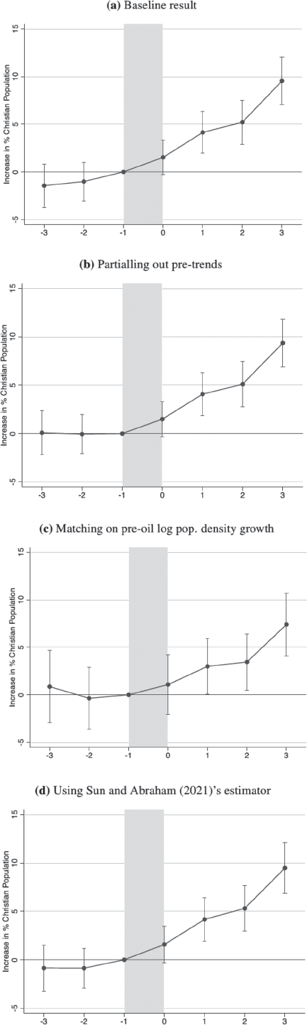
We begin by plotting our baseline event-study estimates in Panel (a) of Figure 4; this corresponds to a more flexible version of the DD estimate in Column (1) of Table 1, which allows us to capture effects beyond a simple level shift and instead reveal interesting dynamics in the treatment effect over time. Post-treatment effects appear somewhat small at first, reflecting heterogeneity in the amount of time since the treatment year as of period 0, and then increase over time thereafter. Following Goodman-Bacon (Reference Goodman-Bacon2021), this pattern raises the possibility that DD estimates are biased toward zero.^{Footnote 24} This is more likely to be the case if estimation relies greatly on time variation, that is, comparisons between different timing groups. Fortunately, our sample contains a large number of never-treated counties, with the Bacon decomposition showing nearly 90 percent of variation used in estimating Equation (1) as coming from comparisons between treated and never-treated units, and DD estimates using only this variation to be 7.75.

Figure 4.

OIL AND RELIGION: EVENT STUDY PLOTS

Notes: Coefficient plots from event-study difference-in-differences analyses that regress membership in 15 major, mainstream Christian denominations (% population) in a county on both year and county fixed effects as well as an indicator for a major oil discovery in the county interacted with event time fixed effects. Panel (d) adopts the estimator proposed by Sun and Abraham (Reference Sun and Abraham2021) to remove contamination from other treatment timing cohorts in the presence of heterogeneous treatment timing. Major oil discoveries are defined as oilfields holding 100 million barrels of oil or more. Event time is defined as the three periods before and after the occurrence of the first major oil discovery. The omitted baseline period is t = −1, which is the last pre-treatment period. The gray shaded area indicates the time frame within which oil is discovered between t = −1 and t = 0. The sample consists of counties in Louisiana, Oklahoma, and Texas, as well as surrounding counties in Alabama, Arkansas, Colorado, Florida, Kansas, Mississippi, Missouri, New Mexico, and Tennessee, covering the nine church and religious censuses held between 1890 and 1990. We exclude counties that are adjacent to oil counties to limit spillover effects that might dilute the treatment. Standard errors are clustered at the county level and error bars represent 95% confidence intervals.

Source: Data on the locations of major U.S. oilfields come from the Oil and Gas Journal Data Book (2000). We link major oilfields with data for all county-oilfields from the Oil and Gas Field Code Master List (U.S. Department of Energy 2004). Church membership data are available via the Association of Religion Data Archives (ARDA). Data for population density come from the U.S. Census of Population, compiled by Haines (Reference Haines2010).

The relatively lesser importance of time variation in our setting is corroborated by robustness exercises showing DD estimates to be largely unchanged when alternative treatment years are used, changing treatment timing. Besides our preferred treatment definition, in which the treatment “switches on” the year a county discovers its first major oilfield, we construct four alternative measures: (i) the year any oil at all is discovered in a county; (ii) the year it or an adjacent oil-abundant county discovers a major oilfield, whichever is first; (iii) the first year any of its major oilfields are discovered in any county, even if not in that county; and (iv) the first year any county in the set of oil-abundant counties with which it is contiguous discovers a major oilfield. Despite these increasingly conservative definitions, Online Appendix Table A3 shows estimates to be highly stable, varying by no more than half a percentage point.

Whereas post-treatment effects are increasing, Panel (a) shows an absence of statistically significant pre-treatment effects. We perform three supplementary event-study exercises to further rule out anticipatory effects. The first two exercises entail basic extensions of Equation (2). Although one common strategy is to control for county-specific linear time trends, this is likely to dilute estimates of dynamic treatment effects in the presence of increasing effects over time. Goodman-Bacon (Reference Goodman-Bacon2021) proposes an alternative strategy in which pre-treatment trends are estimated and then subtracted from the outcome for all periods. This approach can be seen in Panel (b) of Figure 4. Implementing this in our main specification from Table 1 decreases estimates somewhat to 4.9 (.9) pp, which remains highly significant.

A second exercise involves modifying the estimation strategy to compare treated and control counties with similar pre-treatment activity. This involves matching on pre-treatment trends in log population size or density via propensity score matching and the use of matched-pair fixed effects. These exercises tend to flatten pre-trends while generating modest decreases in DD estimates relative to our main specification. One such example can be seen in Panel (c) of Figure 4, which matches on pre-treatment growth trends in log population density. Implementing this yields a smaller DD estimate of 4.0 (1.3) pp. DD estimates from all pre-treatment matching exercises can be found in Online Appendix Table A4.

The third exercise employs an alternative event-study estimator that is robust to heterogeneous treatment timing. Sun and Abraham (Reference Sun and Abraham2021) show that when treatment effects are heterogeneous in settings with heterogeneous treatment timing, pre-trend tests based on standard event-study estimates are invalid. As in Goodman-Bacon (Reference Goodman-Bacon2021), this is driven by contamination from the use of different timing groups as controls alongside never-treated units. They propose an alternative estimator that relies only on never-treated counties as controls. Estimates from this approach can be found in Panel (d) of Figure 4. Post-treatment estimates are highly similar to those from OLS, while pre-treatment estimates are small and statistically insignificant, with minimal trend.^{Footnote 25}

OTHER ROBUSTNESS

A potential inference issue involves spatial correlation in the disturbance ε _ct, which is likely to span beyond individual counties c. We adopt several approaches to account for these. First, we estimate standard errors from Conley (Reference Conley1999), which generate smaller standard errors than specifications that cluster standard errors, as shown in Online Appendix Table A5. Second, we estimate effects using standard errors clustered at trans-county levels of aggregation, at which the treatment is likely to have occurred in practice. These standard errors are slightly larger, but estimates remain highly significant, as shown in Online Appendix Table A6.

Another issue involves heterogeneity of effects across space and sample year. We re-estimate Equation (1), excluding each state and year one at a time, and observe how the oil abundance effect changes from our baseline result. Online Appendix Figure A4 plots the coefficients from this exercise. In no case does excluding any given state or year significantly change the estimated coefficient relative to the baseline result. This is also reassuring regarding our use of time-invariant county boundaries since dropping states with several county boundary changes over time does not change the results.^{Footnote 26}

A final issue involves the construction of the outcome variable. Because our measure of religious participation requires the same set of Christian denominations across all years, some groups are inevitably excluded—most notably the predominantly-Black National Baptist Convention. Since the 1906 Religious Census reports National Baptists in combination with the Northern and/or Southern Baptists for each county, we report in Online Appendix Table A7 estimates using different versions of our outcome variable, which either impute Baptist counts from other years or drop 1906 and Baptist denominations entirely. These result in no substantive change to our estimates.

RELIGIOUS COMMUNITIES AS SOCIAL INSURANCE

Having established that major oil discoveries predict large and persistent increases in the rate of church membership in the oil-rich U.S. South over the twentieth century, we now turn to our favored explanation for this effect. In this section, we explore to what extent religious communities emerged specifically as a form of social insurance. We begin by examining whether treatment effects are rooted in the risk associated with oil abundance. We then consider whether demand for religious communities stems from their provision of actual economic support.

OIL RISK DRIVES RELIGIOUS PARTICIPATION

Downturns in the oil market may generate substantial economic distress for oil communities.^{Footnote 27} Uncertainty in the presence of such shocks may trigger increased religious participation as a form of social insurance, to the extent that the major denominations we study span multiple regions with idiosyncratic risk.^{Footnote 28} To test this, we first establish the importance of oil risk in driving our treatment effects using volatility in oil prices and variation in non-oil economic activity.

OIL PRICE VOLATILITY AND TREATMENT EFFECTS

To capture volatility in world oil prices at a given point in time, we use running standard deviations (st. dev.) of real crude oil prices (in 2018 USD) over preceding 5, 10, and 25 year periods. A larger st. dev. implies greater price volatility. Because crude oil prices are determined by the world market, their fluctuations are largely exogenous to the conditions in any individual oil county. We then interact this measure of volatility with the treatment indicator in Equation (1) to capture the interaction effects of oil volatility on religious participation in oil-abundant counties relative to non-oil counties.

Table 2 shows these interaction effects using the preferred “donut” specification with two-way fixed effects and no other controls. Estimates reveal that a one st. dev. increase in oil price volatility coincides with treatment effects that are about 24 percent larger—consistent with our hypothesis—with larger and more precise interaction effects coming from longer-run measures of volatility.^{Footnote 29}

Table 2

HETEROGENEOUS EFFECTS: OIL PRICE VOLATILITY

Notes: Estimates are from difference-in-differences regressions of membership in 15 major, mainstream Christian denominations (% population) in county c in year t on an indicator called “oil abundance,” which equals one for a county in years following a major oil discovery and is zero otherwise. Major oil discoveries are defined as oilfields holding 100 million barrels of oil or more. The sample consists of counties in Louisiana, Oklahoma, and Texas, as well as surrounding counties in Alabama, Arkansas, Colorado, Florida, Kansas, Mississippi, Missouri, New Mexico, and Tennessee, covering the nine church and religious censuses held between 1890 and 1990. We exclude counties that are adjacent to oil counties to limit spillover effects that might dilute the treatment. All regressions include county and sample year fixed effects. The additional regressors include interactions of the oil abundance indicator with the standard deviation of world per barrel real (2018 USD) oil prices (Columns (1)–(3)) and of the log world oil price (Columns (4)–(6)) over 5, 10, and 25 years as measures of income risk associated with oil. Standard errors are clustered at the county level. Significance levels are denoted by *p<0.10, **p<0.05, ***p<0.01.

Sources: Data on the locations of major U.S. oilfields come from the Oil and Gas Journal Data Book (2000). We link major oilfields with data for all county-oilfields from the Oil and Gas Field Code Master List (U.S. Department of Energy 2004). Church membership data are available via the Association of Religion Data Archives (ARDA). Oil price data was compiled by BP and collected from Quandl at https://www.quandl.com/data/BP/CRUDE_OIL_PRICES (accessed 27 July 2020).

One concern is that oil prices tend to be higher in times of high volatility, with short-term positive shocks to oil price levels driving this effect rather than the volatility in prices per se. To test this, we include in Online Appendix Table A9 lagged demeaned real price level interactions alongside the volatility interactions. This generally sustains our estimates of the latter’s effects.

OIL DEPENDENCE AND TREATMENT EFFECTS

Crude oil prices are not the only source of risk faced by oil communities. When the Texas oil boom began at the turn of the twentieth century, much of Texas was sparsely populated, and neither Oklahoma nor New Mexico were U.S. states. And although major agglomerations often sprung up around oil boomtowns (Michaels Reference Michaels2011), many oil communities in the sample remained highly oil-dependent throughout the twentieth century—and arguably would have remained sparsely populated in the absence of oil’s riches. To the extent that oil is the primary source of wealth and urban growth in many parts of the U.S. South and Southwest, the local economic risk entailed by oil abundance may be amplified even more in those places. This in turn may have contributed to the treatment effects observed previously, driving even greater reliance on religious communities for economic support during oil downturns.

To capture heterogeneous effects from greater dependence on oil, we develop several time-invariant variables with which to interact the treatment dummy. These variables capture non-oil economic activity at the start of the event window, when to-be-treated and never-treated counties were similar on average. The first two capture the extent of urbanization at the start of the Oil Age. One of these is a continuous variable, measuring log population density in 1900. Another is a dummy capturing whether a county contained part of an urban agglomeration with a population of at least 25,000 in 1890. To the extent that a county had high levels of urbanization prior to discovering oil, its economic performance would likely be less dependent on oil’s bounty.

The second set of variables captures a county’s manufacturing activity prior to oil’s discovery. The first measures log manufacturing output per capita in 1900. The second is a dummy indicating above-sample-median manufacturing output in 1900. Having a larger manufacturing presence implies lower aggregate risk: not only does it mean a place has historically had economic activity independent of oil, but manufacturing also serves as a key substitute sector for mining labor during oil downturns.^{Footnote 30}

The third set of variables captures a county’s cotton activity prior to oil’s discovery, using a continuous measure of the share of land used for cotton in 1900 and a corresponding above-sample-median cotton dummy. Cotton in itself was a source of economic risk throughout the South in the early twentieth century, but this risk was driven by different sources than oil’s, such as the boll weevil. Hence, cotton-rich places that have discovered major oil might have smaller treatment effects due to risk diversification.

Consistent with oil dependence driving economic risk, treatment effects are significantly larger in more oil-dependent counties with smaller pre-discovery populations, manufacturing sectors, and cotton density. Estimates produced from these interactions, as shown in Online Appendix Table A10, reveal that treatment effects are driven by counties without an urban presence prior to oil’s discovery—with a one st. dev. increase from the sample mean in log population density in 1900 reducing treatment effects to zero—and reduced significantly by the pre-oil presence of manufacturing and cotton. This suggests effects are being driven largely by higher-risk “boomtowns” whose economic activity stems from oil.

PRIVATE AND PUBLIC SUBSTITUTES

Although religious participation appears to increase in response to oil’s economic risk, it is possible such effects are rooted in psychological forms of support rather than economic ones. Indeed, evidence for “religious coping” has been documented in recent work by Bentzen (Reference Bentzen2019). While we consider the role of religious coping later in the paper, we first provide evidence that religious communities indeed provide economically meaningful forms of social insurance demanded in response to oil risk.

To show this, we first examine key substitutes in the provision of insurance. If religious participation emerges in oil counties in response to increased demand for social insurance, one would expect a greater supply of private and public substitutes for smoothing consumption, with more complete contracts, to crowd out relative increases in religious participation in oil counties (Hungerman Reference Hungerman2005; Chen Reference Chen2010). We begin by examining public insurance substitutes in the form of state-provided social insurance.

OIL AND RELIGION IN THE PUBLIC SOCIAL INSURANCE ERA

Public social insurance first became widespread in the U.S. in the 1930s but continued to vary by state thereafter, with Southern states generally providing less. Hence, to study interaction effects from public social insurance, we interact our county-level oil abundance indicator with time- and state-varying measures of maximum weekly (i) unemployment insurance and (ii) workers compensation benefits from Fishback (Reference Fishback2020). These measures are each adjusted to reflect relative value, using the ratio of benefits to either (i) the national poverty line weekly income equivalent for a 4-person family; (ii) average weekly earnings plus benefits for manufacturing workers in the state; or (iii) state weekly per capita income.

As shown in Table 3, we find that the introduction of public social insurance benefits comparable to national poverty line income standards reduces effects by nearly two-thirds. When it is available at levels comparable to even higher standards, such as average state incomes or manufacturing earnings, positive effects of oil on religious participation disappear entirely, although availability to this extent is seldom the case in our sample. This mirrors previous findings by Gruber and Hungerman (Reference Gruber and Hungerman2007) showing a reduction in charitable giving by churches following the New Deal.

Table 3

HETEROGENEOUS EFFECTS: ACCESS TO PUBLIC SOCIAL INSURANCE

Notes: Estimates are from difference-in-differences regressions of membership in 15 major, mainstream Christian denominations (% population) in county c in year t on an indicator called “oil abundance,” which equals one for a county in years following a major oil discovery and is zero otherwise. Major oil discoveries are defined as oil fields holding 100 million barrels of oil or more. The sample consists of counties in Louisiana, Oklahoma, and Texas, as well as surrounding counties in Alabama, Arkansas, Colorado, Florida, Kansas, Mississippi, Missouri, New Mexico, and Tennessee, during the post-New Deal period when states had developed social insurance systems. We exclude counties that are adjacent to oil counties to limit spillover effects that might dilute the treatment. All regressions include county and sample year fixed effects. The additional regressors are interactions of the oil abundance indicator with measures of state-level maximum weekly unemployment insurance and workers compensation benefits, beginning in 1940 through 1990, each of which is adjusted to reflect relative value by (i) national poverty line weekly income equivalent for a four-person family, (ii) average weekly earnings plus benefits for manufacturing workers in the state, and (iii) state weekly per capita income, respectively. Standard errors are clustered at the county level. Significance levels are denoted by *p<0.10, **p<0.05, ***p<0.01.

Sources: Data on the locations of major U.S. oilfields come from the Oil and Gas Journal Data Book (2000). We link major oilfields with data for all county-oilfields from the Oil and Gas Field Code Master List (U.S. Department of Energy 2004). Church membership data are available via the Association of Religion Data Archives (ARDA). Public insurance data from come from Fishback (Reference Fishback2020).

ACCESS TO CREDIT AND PRIVATE INSURANCE

Do oil counties that had greater access to credit and private insurance prior to oil’s discovery exhibit similar “crowd out” effects to that observed with public social insurance? To answer this, we use data on historical credit availability—as measured by the number of savings and loan associations and bank tellers in each county—as well as on private insurance—as measured by the number of insurance agents and brokers in each county. As a large number of counties report having zero of these, we generate a dummy variable for each, indicating whether a county had any prior to treatment.

Due to limitations in how far back credit availability data go, in our preferred specifications, we drop some treated counties to reduce “bad control” concerns. In particular, savings and loan associations became prominent throughout the United States following the Federal Home Loan Bank Act of 1932, and county-level data for them first corresponds to our religious census dataset in 1950. County-level data on bank tellers and insurance agents, meanwhile, are available for the full set of sample counties starting in 1910. Our main specifications thus drop counties treated prior to 1950 when examining heterogeneous effects from savings and loan banks and pre-1910 for bank tellers and private insurance.

Estimates for these are reported in Table 4 and are again consistent with a “crowd out” hypothesis. In particular, having a savings and loan association or access to bank tellers reduces effects almost entirely in specifications that drop previously treated observations, as shown in Columns (1b) and (2b), respectively. Meanwhile, effects are more than halved for counties with access to private insurance, as shown in Column (3b). Effects are robust to including all observations instead, as shown in the remaining columns. Overall, this suggests religious communities are indeed engaged in the provision of social insurance, primarily in the absence of private substitutes.

Table 4

HETEROGENEOUS EFFECTS: ACCESS TO CREDIT AND PRIVATE INSURANCE

Notes: Estimates are from difference-in-differences regressions of membership in 15 major, mainstream Christian denominations (% population) in county c in year t on an indicator called “oil abundance,” which equals one for a county in years following a major oil discovery and is zero otherwise. Major oil discoveries are defined as oilfields holding 100 million barrels of oil or more. The sample consists of counties in Louisiana, Oklahoma, and Texas, as well as surrounding counties in Alabama, Arkansas, Colorado, Florida, Kansas, Mississippi, Missouri, New Mexico, and Tennessee, covering the nine church and religious censuses held between 1890 and 1990. We exclude counties that are adjacent to oil counties to limit spillover effects that might dilute the treatment. All regressions include county and sample year fixed effects. We interact the oil abundance indicator with indicators for alternative insurance possibilities, such as banks and private insurance companies. Those include dummies for whether a county had any savings and loan associations in 1950, or whether there were any bank teller or insurance agents in the county in 1910. The latter two variables come from the full-count Census of 1910, while data on savings and loan associations were not available in the U.S. Census County Data Books until the mid-nineteenth century. To minimize bad control concerns, secondary specifications in all Columns (b) exclude counties treated prior to the year of the interaction term. Standard errors are clustered at the county level. Significance levels are denoted by *p<0.l0, **p<0.05, ***p<0.0l.

Sources: Data on the locations of major U.S. oilfields come from the Oil and Gas Journal Data Book (2000). We link major oilfields with data for all county-oilfields from the Oil and Gas Field Code Master List (U.S. Department of Energy 2004). Church membership data are available via the Association of Religion Data Archives (ARDA). Data for controls come from the U.S. Census of Population, compiled by Haines (Reference Haines2010).

Given the attenuation of effects from the supply of private substitutes, one might also expect demand for these to increase with oil abundance, all else fixed. To measure demand for private banking as used for smoothing consumption, we use two continuous measures of savings as outcomes: log savings capital in savings and loan associations per capita and log time deposits per capita. To measure demand for private insurance, we use the logged number of insurance agents and brokers per capita.

These results are again consistent with the notion of religious communities and private banking or insurance as substitutes. Online Appendix Table A11 shows oil abundance increases demand for savings capital and time deposits by nearly 10 percent, while increasing the number of insurance agents and brokers per capita by nearly 50 percent. Note that, as many counties lack these outcomes, results are somewhat sensitive to including zero-valued counties.

One concern is that the results in Table 4 and Online Appendix Table A11 do not reflect quantities of these private substitutes but rather are merely correlates of urban growth. For instance, a place with no insurance agents is likely to be rural and thus more religious. We replicate Table 4 but control for pre-treatment log population density in 1950 and 1910 to probe for robustness for Columns (1a–b) and (2a–3b), respectively. The results are reported in Online Appendix Table A12. Though interaction effects are reduced, neither main nor interaction effects lose statistical significance. Online Appendix Table A13 performs a similar exercise for the regressions in Online Appendix Table A11, controlling for time-varying log population density to test whether post-oil urban growth captures the relevant variation driving increases in outcomes in Table A11. The only effect that loses statistical significance is for the log number of insurance agents per capita when zero-valued counties are included. Altogether, this suggests log population density and urbanization during the sample period are not driving these findings.

DO RELIGIOUS COMMUNITIES SMOOTH ECONOMIC VOLATILITY?

Now that we have shown that religious communities exhibit substitutability with other insurance mechanisms in oil-abundant settings, we consider whether relative fluctuations in economic outcomes following oil price shocks are indeed smaller in oil counties when a large religious community is present. To do this, we compare how relative labor outcomes in oil counties respond to oil price shocks when religious participation is above versus below the sample median, using our measure of Christian membership in 1936 and a subsample of already- and never-treated counties spanning 1940 to 1990.^{Footnote 31}

Consistent with the historical importance of churches in providing economic aid—recall that in 1926, U.S. churches spent $150 million on social support, compared to $23 and $37 million by state and local governments—as well as other services such as job training and employment matching, relative increases in unemployment in oil counties after a negative oil price shock are significantly smaller when a large religious community is present. Table 5 shows that, whereas a negative oil price shock of $30 2018 USD (i.e., about a sample standard deviation) increases the unemployment rate in an oil-abundant county relative to non-oil county by 1 p.p. among below-median Christian counties, the same shock increases relative unemployment by only 0.7 p.p. among above-median Christian counties, with the difference between these coefficients being highly statistically significant.

Table 5

OIL PRICE SHOCKS, RELIGIOUS COMMUNITIES, AND LABOR OUTCOMES, 1940–90

Notes: Estimates are from regressions of county-level economic outcomes in county c in year t on an “oil” indicator, which equals one if and only if a county lies above an oilfield holding 100 million barrels of oil or more. This oil dummy is interacted with a time-varying measure of world per barrel crude oil prices (in 2018 USD). This term is interacted with a time-invariant indicator of whether a county was above the sample median in Christian membership in 1936. This year was chosen because most outcomes are reported in the U.S. Census County Data Books beginning in 1940. We therefore exclude counties treated after 1936, which, as such, may see increases in Christian participation later in the panel, thus biasing estimates. The sample consists of counties in Louisiana, Oklahoma, and Texas, as well as surrounding counties in Alabama, Arkansas, Colorado, Florida, Kansas, Mississippi, Missouri, New Mexico, and Tennessee, and is decadal from 1940 to 1990. We exclude counties that are adjacent to oil counties to limit spillover effects that might dilute the treatment. All regressions include county and sample year fixed effects. Outcomes include log population density, shares of labor force in mining, agriculture, and manufacturing, and the unemployment rate. Standard errors are clustered at the county level. Significance levels are denoted by *p<0.10, **p<0.05, ***p<0.01.

Sources: Data on the locations of major U.S. oilfields come from the Oil and Gas Journal Data Book (2000). We link major oilfields with data for all county-oilfields from the Oil and Gas Field Code Master List (U.S. Department of Energy 2004). Church membership data are available via the Association of Religion Data Archives (ARDA). Data for outcomes come from the U.S. Census of Population, compiled by Haines (Reference Haines2010).

To what extent is this rooted in reduced consumption volatility? The rest of Table 5 suggests that religious communities indeed achieve this by limiting the spread of demand shocks beyond the oil sector. Following a negative oil price shock, oil counties with relatively small religious communities tend to experience out-migration, and the local agricultural sector suffers, while manufacturing becomes relatively more important for local labor demand. In oil counties with relatively large religious communities, however, migratory patterns remain flat relative to non-oil counties, and relative fluctuations in agricultural and manufacturing employment are both reduced by about two-thirds. This is consistent with the notion that material aid and provision of labor market matching services by religious communities may smooth the local effects of income shocks in oil counties—not only for oil workers but for their communities.

An alternative explanation for these findings might be that counties with large religious communities are more economically diversified. This would explain these heterogeneous effects independently of the social insurance channel. Contrary to this explanation, we find that sample counties with large religious communities tend to have more industry concentration. Greater industry and occupational concentration at the county level as of 1900 similarly appear to increase the relationship between oil and religion, although these estimates are not significant. These results can be found in Online Appendix Table A15.

EVIDENCE FROM DENOMINATIONAL RESPONSES

Further evidence that effects are driven by increased demand for social insurance can be found by looking at different denominational responses to oil discoveries, including (i) changes in competition among denominations and (ii) relative changes in participation among denominations that are more versus less likely to efficiently provide social insurance.

Column (1) of Online Appendix Table A16 shows that oil abundance decreases the concentration of different Christian denominations in our sample of denominations by about 3.8 percent. This makes sense: a positive demand shock for the goods and services provided by religious communities (i.e., social insurance) may trigger new entrants into the market for religion and spur all denominations, including pre-existing ones, to increase their level of effort, increasing religious participation across multiple denominations (Iyer Reference Iyer2016). Online Appendix Figure A5 shows the dynamic nature of this process, which mirrors the increasing nature of our main treatment effects in Figure 4. This is consistent with increased demand for social insurance and subsequent market entry, increasing the equilibrium quantity of social insurance over time.

Which denominations are behind this effect? In theory, it should be the best provider of social insurance. We examine the three most prominent groups in our sample of the U.S. South: Roman Catholics, Southern Baptists, and United Methodists. We find sizable and significant membership increases following major oil discoveries for only the first two, as shown in Online Appendix Table A16. This is consistent with club models of religion in which joining a religious community entails access to certain goods and services (e.g., social insurance) in return for the costs entailed by membership. More liberal denominations with fewer such membership costs (e.g., less sacrifice), particularly mainline Protestant denominations such as Methodists, in turn, tend to entail greater “free-riding” with respect to such goods, at the expense of their provision to members (Iannaccone Reference Iannaccone1992).^{Footnote 32} A demand shock for social insurance would therefore not necessarily generate an increase in membership among Methodists relative to Southern Baptists. Catholics, meanwhile, are ideologically mixed, having become more liberal overall since the Vatican II reforms but remaining quite conservative in the Gulf Coast South, that is, in the heavily Catholic parts of our sample (Iannaccone Reference Iannaccone1994).

There are nonetheless key differences between Catholics and Southern Baptists. Catholics tended to focus their aid on urban areas, in which 4 percent of total church expenditures in 1936 went toward local relief and charity versus about 2.1 percent in rural areas (U.S. Census Bureau 1936). Meanwhile, Southern Baptists invested more in rural areas, with 3.2 percent of expenditures going to local relief and charity in such places versus 1.9 percent in urban areas. These comparative advantages reflect their membership: only 19.4 percent of Catholics in 1936 were rural versus 62.1 percent of Southern Baptists. The heatmaps in Figure 5 show the spatial differentiation of Catholics and Southern Baptists early in the event window.

Figure 5

SPATIAL DISTRIBUTION OF DENOMINATIONS IN 1916

Notes: Maps show the spatial distribution of different Christian denominations as a share of the total population in our sample counties, as reported in the 1916 United States Census of Religious Bodies. Oil-abundant counties are outlined in black, while urban areas (cities with population >100,000 in 2019) are dotted. Note the sudden decline in Southern Baptists at the Kansas border, which generally marks the edge of the Bible Belt.

Sources: City population and longitude-latitude data from SimpleMaps.com at https://simplemaps.com/data/us-cities (accessed 20 August 2020). Church membership data are available via the Association of Religion Data Archives (ARDA).

After WWII, Catholics continued to cluster along the Gulf Coast and near Mexico, while Southern Baptists became increasingly dominant throughout the remaining Southern counties in our sample, as shown in subsequent heatmaps in Online Appendix Figures A6 and A7. Indeed, most of the increase in overall membership observed in our data stems from the latter’s growth.^{Footnote 33} Of this growth, a disproportionate amount occurred in oil counties: Southern Baptist membership grew 437 percent in oil-abundant counties between 1906 and 1990, compared to 244 percent in control counties.^{Footnote 34} The heatmaps also show the relative stagnation of the Methodists, whose conservative Southern groups joined the more liberal Methodist Episcopalians in 1939.

EXPLORING OTHER MECHANISMS

In this final section, we explore several additional channels, besides social insurance, through which oil reliance may have prompted increases in religious participation. First, major oil discoveries may have spurred selective migration by more religious types. Second, local economic development driven by oil discoveries may have coincided with changes that explain oil’s effect on religious participation. Third, risk associated with oil may also have generated increases in religiosity through a psychological religious coping channel independent of the economic support offered by religious communities. We consider these now.

SELECTIVE MIGRATION

Ideally, we would implement an experiment that randomly endows one of two similar populations of fixed size and composition with oil and related industries, and then we would measure how patterns of religious participation change differently across them. In practice, however, many of those living in oil-abundant counties are likely to have migrated there following oil’s discovery and subsequent increases in labor demand. This raises the possibility that observed increases in religious participation are actually the outcome of compositional change among the population following the discovery of oil, driven by migratory sorting among more religious types.

To test for this possibility, we examine whether an individual’s religious characteristics predict their migration to oil-abundant counties following the discovery of oil in both the short and long run. To measure the religious characteristics of migrants, we follow Anderson and Bentzen (Reference Anderson and Bentzen2021) and use the given names of their born children. Names are considered “Biblical names” if they match or are phonetically related to names featured in the Old or New Testament, as listed on behindthename.com. Table 6 shows the most common Biblical and non-Biblical names in our dataset. Our sample of migrants to Southern oil and non-oil counties is derived from the “residence in 1935” question in the 1940 U.S. Census, which associates census respondents with their migration status between 1935 and 1940, when the Southern oil boom was at its peak (see Figure 3).^{Footnote 35} Given this, we consider the names of unmarried children between the ages of 5 and 18 as of 1940, who would have been named prior to 1935 and thus had names indicative of the pre-migration religious characteristics of migrating household heads. As a validation check on the religious signal of Biblical names in this exercise, we show in Online Appendix Table A17 that among migrant households in 1940, having a child with a Biblical name predicts living in a county with about 0.5 percent higher rates of Christian church membership, relative to the sample mean.^{Footnote 36}

Table 6

TOP BIBLICAL AND NON-BIBLICAL NAMES IN 1940

Notes: Names are based on groupings of phonetically similar names as determined by both the NYSIIS and Soundex phonetic coding algorithms. A few popular names—such as Margaret, Henry, and Dorothy, which each make up just under a percent of the sample—are designated as religious names by Soundex but not by NYSIIS. The reverse is not true. None of these have Biblical or otherwise Christian roots. On this basis, we treat NYSIIS as our preferred phonetic device but report estimates in Table 7 from both for completeness.

Source: Tables shows the rank and frequency of the top ten most common Biblical and non-Biblical names in the 1940 names sample from the U.S. Census, using the list of names in the Bible from behindthename.com.

To examine whether more religious types are more likely to sort into counties following major oil discoveries, we first regress an indicator for whether a child’s household head moved between 1935 and 1940 to a county in which a major oil discovery was made during that period on an indicator for whether that child had a Biblical name. We exclude counties in which oil was discovered prior to 1935, such that migrants to oil-abundant counties are compared only to individuals who never selected into an oil-abundant county. To minimize spillover effects (e.g., from commuters), we also dropped non-oil counties adjacent to known oil-abundant counties as of 1940. We control for state fixed effects as well as dummies for a child’s age, race, sex, and place of birth. Standard errors are clustered at the household level. In secondary specifications, we also dummy for whether the household head worked in oil.

In nearly all cases, we find evidence consistent with negative selection, in which household heads with Biblically-named children are somewhat less likely to move to newly oil-abundant counties. This is consistent with the notion that correlates of urban growth are often negatively correlated with religious participation. In contrast, household heads working in oil select positively into newly oil-abundant counties. These estimates are shown in Columns (1)–(4) of Table 7.

Table 7

DOES SELECTIVE MIGRATION DRIVE EFFECTS?

Notes: Estimates are from regressions of an indicator for whether a child’s household head moved between 1935 and 1940 to an oil-abundant county on an indicator for whether that child had a Biblical name. A county is considered oil abundant if it lies above a known major oil field, holding 100 million barrels of oil or more. The sample consists of all unmarried children between the ages of 5 and 18 in 1940 who resided as of that year in counties in Louisiana, Oklahoma, and Texas. We exclude counties that are adjacent to known oil counties to limit spillover effects that might dilute effects, as well as counties treated prior to 1935 in Columns (1)–(4) and children of households who moved to counties treated between 1935 and 1940 in Columns (5)–(6). All regressions include state-fixed effects. We also control for dummies for the child’s age, race, sex, and place of birth. Standard errors are clustered at the household level. Significance levels are denoted by *p<0.l0, **p<0.05, ***p<0.0l.

Source: Data on the locations of major U.S. oilfields come from the Oil and Gas Journal Data Book (2000). We link major oilfields with data for all county-oilfields from the Oil and Gas Field Code Master List (U.S. Department of Energy 2004). Church membership data are available via the Association of Religion Data Archives (ARDA). Individual-level data come from Ruggles et al. (Reference Ruggles, Sarah Flood, Josiah Grover, Pacas and Sobek2018).

Even if we observe no evidence of migratory sorting by religious types in our baseline regression, there may still be selective migration occurring among later movers. This might even account for our increasing treatment effects in event studies. We therefore also examine whether religious characteristics predict migration between 1935 and 1940 to counties in which major oilfields were discovered prior to 1935. We regress an indicator for whether a child’s household head moved between 1935 and 1940 to a county in which major oil was discovered prior to 1935 on an indicator for whether that child had a Biblical name. We exclude migrants from counties that were treated between 1935 and 1940, as well as migrants from oil-adjacent counties. These estimates, shown in Columns (5) and (6) of Table 7, are similar in sign and size to those associated with migrants to newly oil-abundant counties, suggesting that selective migration by religious types is not driving our treatment effects over the short or long run.

We consider four extensions of this exercise. The first excludes children of non-migrants from the sample, such that the religious characteristics of migrants are compared only to those of other migrants to (non-adjacent) never-treated or non-yet-treated counties. Estimates are ultimately not sensitive to who we include. These results can be found in Online Appendix Table A18. Second, we consider sensitivity to phonetic coding and estimate a version that limits the set of names to those coded the same (e.g., as Biblical) across both NYSIIS and Soundex phonetic algorithms. Results are relatively unchanged in this smaller sample. These results can be found in Online Appendix Table A19. Third, we consider a sample that sets the maximum age of children at 10, following Bazzi, Fiszbein, and Gebresilasse (Reference Bazzi, Fiszbein and Gebresilasse2020). These estimates, shown in Online Appendix Table A20, are unchanged as well. Fourth, we address the fact that this exercise only considers migrants with children and estimate a version of Table 7 that examines, among a subsample of single household heads with no children, whether having a Biblical name oneself predicts migration to an oil-abundant county. These results, which can be found in Online Appendix Table A21, again show no significant positive relationship between Biblical names and selective migration to oil-abundant counties.

LOCAL ECONOMIC DEVELOPMENT

Another possibility is that economic development associated with oil discoveries was tied to a number of important changes locally, such as population size and agglomeration, income growth, and educational attainment (Michaels Reference Michaels2011). These are potentially relevant factors, whose changes may explain some or even all of oil’s effect on religious participation. For instance, a substantial body of literature has studied how religious participation changes alongside education and income.^{Footnote 37}

To address this, we first examine whether changes in education, income, population size, or population composition capture the relevant variation in our treatment variable, by including them as controls in our main regression. Table 8 confirms that many of these variables are relevant. We find a negative and significant relationship between educational attainment and religious participation, as well as a negative relationship for income, similar to Becker and Woessmann (Reference Becker and Woessmann2013) in the Prussian context. At the same time, neither variable explains away or meaningfully alters the treatment effects. Columns (3)–(5) consider alongside these the inclusion of various population size and compositional controls, again with little consequence to our treatment effects. These are instructive, as they suggest our effects are not driven by agglomeration or compositional effects from oil discoveries. Column (3), for instance, takes into account the extensive margin of population change. Especially in the earlier sample periods, increases in population size were mainly driven by the inflow of new people rather than new births. Column (4) takes into account the intensive margin. Reaffirming the selective migration exercise from the previous section, changes in compositional factors result in little change in estimates.

Table 8

DO CHANGES IN EDUCATION, INCOME, OR POPULATION EXPLAIN TREATMENT EFFECTS?

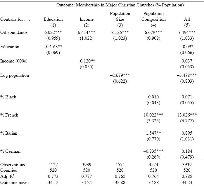
Notes: Estimates are from difference-in-differences regressions of membership in 15 major, mainstream Christian denominations (% population) in county c in year t on an indicator called “oil abundance,” which equals one for a county in years following a major oil discovery and is zero otherwise. Major oil discoveries are defined as oilfields holding 100 million barrels of oil or more. The sample consists of counties in Louisiana, Oklahoma, and Texas, as well as surrounding counties in Alabama, Arkansas, Colorado, Florida, Kansas, Mississippi, Missouri, New Mexico, and Tennessee, covering the nine church and religious censuses held between 1890 and 1990. We exclude counties that are adjacent to oil counties to limit spillover effects that might dilute the treatment. All regressions include county and sample year fixed effects. To measure educational attainment, we use the percentage of adults (aged 25 plus) with a high school degree. As these are not available for 1926 and prior, we use the literacy rate for those years. To measure income, we use median family income in 2018 dollars. As income data are not available for 1926 and prior, we rely on another commonly used metric for those years based on occupational income scores. This score is computed based on the median income in a given occupation in 1950, assigned to individuals’ occupations in previous years to proxy for their income. For the 1906, 1916, and 1926 religious census years, we average those income scores by county based on the full-count Census files. Estimates using only the period from 1936 are qualitatively similar and available upon request. Columns (3) and (5) control for log population to capture factors associated with urbanization and market size. Columns (4) and (5) control for compositional factors associated with migration. Standard errors are clustered at the county level. Significance levels are denoted by *p<0.10, **p<0.05, ***p<0.01.

Sources: Data on the locations of major U.S. oilfields come from the Oil and Gas Journal Data Book (2000). We link major oilfields with data for all county-oilfields from the Oil and Gas Field Code Master List (U.S. Department of Energy 2004). Church membership data are available via the Association of Religion Data Archives (ARDA). Data for controls come from the U.S. Census of Population and Housing and the Census of Agriculture, compiled by Haines (Reference Haines2010) and Haines et al. (Reference Haines, Fishback and Rhode2018), respectively, together with manufacturing data from Matheis (Reference Matheis2016).

We further probe the robustness of our results with respect to issues of population growth and agglomeration using a series of matching exercises in order to better compare treated counties with control counties that have similar urban growth trajectories. The first of these exercises involves matching and comparing treated and control countries based on pre-treatment trends in population and density growth, using propensity score matching and estimation with matched-pair fixed effects. These estimates can be found in Online Appendix Table A4. While coefficients vary somewhat in terms of size, these matching exercises universally preserve the sign and statistical significance of estimates. Our second set of exercises further deals with the fact that strong agglomeration effects are likely to follow oil discoveries, which may promote church construction. We address this by comparing counties matched on population and manufacturing growth over the full sample, again with little change in estimated treatment effects across specifications, as shown in Online Appendix Tables A22 and A23. Together, these findings suggest oil abundance is affecting religious participation through channels independent of initial and post-oil urban growth.

RELIGIOUS COPING

A third possibility is that oil’s risk is indeed at the heart of the relationship between oil dependence and religious participation, but that increases in the latter are rooted less in economically meaningful forms of social insurance and more in religion’s psychological benefits. The “religious coping” hypothesis involves the use of religion to cope with unpredictable or distressing factors. The relevant benefits from religion in this context are not economic (e.g., material aid and charity), but rather the psychological benefits of prayer and the guidance offered by religious scripture. Religious coping is thus associated with greater intrinsic religiosity—that is, genuine belief—while a social insurance effect may simply entail greater extrinsic religiosity—that is, religious participation prompted by demand for religious services made available through actual churchgoing.

Previous research shows both economic and psychological benefits of religion as salient responses to economic risk and uncertainty (Binzel and Carvalho Reference Binzel and Carvalho2017; Ager and Ciccone Reference Ager and Ciccone2018). Recent work by Bentzen (Reference Bentzen2019) seeks to disentangle these two channels, using earthquake risk—but not direct exposure—to capture the effect of risk independent of physical economic distress. Consistent with the religious coping hypothesis, she documents a large and significant effect of earthquake risk on intrinsic religiosity, as captured by the strength of one’s beliefs and personal relationship with God, while actual churchgoing is unaffected.

We follow Bentzen (Reference Bentzen2019) here and examine the relationship between oil reliance and intrinsic religiosity. We adopt three different measures. First, we use our Biblical names measure from earlier to test whether exposure to oil-abundant counties affects the religious naming of children over the short run. Second, we use two measures of intrinsic religiosity over the long run from the American National Election Survey (ANES), which identifies respondents at the county level over the second half of the twentieth century: (i) whether one attains guidance from religion and (ii) whether one believes in the Bible as the literal word of God. As a placebo, we use churchgoing as a measure of extrinsic religiosity, which we expect to rise in oil-abundant settings as a prerequisite for social insurance provision and receipt.

Similar to Bazzi, Fiszbein, and Gebresilasse (Reference Bazzi, Fiszbein and Gebresilasse2020), the first exercise exploits variation in the probability of exposure to oil reliance at a child’s time of naming, using the sample of migrant households described earlier, to test whether increased exposure to the treatment drives increases in intrinsic religiosity among households moving to recently oil-abundant counties.^{Footnote 38} We estimate two models: one that imposes a linear time trend on exposure effects among migrant children and another that estimates effects using age-specific dummies. These effects are estimated relative to those based on children with no exposure to the treatment at the time of birth because their household moved to a non-oil county or because they were named prior to migrating. All specifications dummy for child age, race, sex, and place of birth, while secondary specifications also control for household fixed effects, using households with multiple children, which absorb all time-invariant characteristics of the household, including its cultural attitudes, its place of origin, and factors affecting its destination choice. Across all specifications, estimated in Online Appendix Table A24, exposure to an oil-abundant county is not associated with any statistically significant differences in naming patterns across migrant children, suggesting no differences in intrinsic religiosity present among those living in oil-reliant settings over the short run.

The second exercise uses survey responses from ANES spanning the second half of the twentieth century to capture potential differences over the longer run in intrinsic religiosity among those residing in oil-abundant counties. On the right-hand side, we use our county-level measure of known oil abundance, while outcome variables include two measures of intrinsic religiosity (“guidance from religion” and “believe in Bible as word of God”) and one measure of extrinsic religiosity (“attend church”). In contrast to Bentzen (Reference Bentzen2019), only extrinsic religiosity appears to differ across oil and non-oil counties in our setting, where living in an oil-abundant county is associated with a 4.3 percent higher probability of being a churchgoer relative to the sample mean. These results can be found in Panel (a) of Online Appendix Table A25. Together, our findings suggest intrinsic religious belief is relatively unaffected by oil reliance, while religious participation increases sharply and remains high over time—more consistent with treatment effects reflecting increased demand for religious benefits made available through churchgoing, such as social insurance. On the other hand, the table also shows in Panel (b) that there do seem to be ideological effects over the long run in a more general sense. These include self-reporting as politically conservative, support for reducing federal environmental spending, and for big business in counties with oil discoveries. This meshes with the work of Dochuk (Reference Dochuk2019), which suggests a complex and multifarious interaction between oil and religious institutions in oil-abundant areas where religious doctrine may have spillovers on these other dimensions. More empirical research should examine these more nuanced channels.