


1. Introduction
Interaction between shock waves and the boundary layer (BL) developing on rigid wings can lead to self-sustained periodic flow oscillations referred to as transonic buffet (Helmut Reference Helmut1974). It can cause strong variations in lift coefficients possibly leading to wing vibrations and structural fatigue or failure. For these reasons, transonic buffet can limit the flight envelope of civilian aircraft and the manoeuvrability of combat aircraft (Roos Reference Roos1980; Lee Reference Lee2001; Giannelis, Vio & Levinski Reference Giannelis, Vio and Levinski2017). Transonic buffet on infinite wing sections (i.e. aerofoil buffet), which we henceforth refer to as ‘buffet’ for brevity, usually occurs at low frequencies, with the Strouhal number based on the chord and freestream velocity,  $St < 1$. Most studies on buffet focus on ‘turbulent buffet’ where a turbulent BL develops well upstream of the shock wave (e.g. due to fully turbulent inflow conditions or forced transition (Jacquin et al. Reference Jacquin, Molton, Deck, Maury and Soulevant2009) or even under free transition conditions at high $\textit {Re}$ (Lee Reference Lee1989)). Although the fundamental mechanisms that drive this buffet type remain unclear (Giannelis et al. Reference Giannelis, Vio and Levinski2017), recent studies have shown that this phenomenon arises through a supercritical Hopf bifurcation associated with an unstable global mode (Crouch, Garbaruk & Magidov Reference Crouch, Garbaruk and Magidov2007; Crouch et al. Reference Crouch, Garbaruk, Magidov and Travin2009; Sartor, Mettot & Sipp Reference Sartor, Mettot and Sipp2015; Crouch, Garbaruk & Strelets Reference Crouch, Garbaruk and Strelets2019; Timme Reference Timme2020). In contrast to turbulent buffet, relatively few studies have examined ‘laminar buffet’, for which the BL remains laminar from the leading edge until approximately the shock foot location. The mechanisms governing laminar buffet have been proposed to be distinct from those governing turbulent buffet (Dandois, Mary & Brion Reference Dandois, Mary and Brion2018). Further, the effects of various flow parameters on laminar buffet remain largely unexplored. Motivated by these open questions, we examine the influence of flow parameters on laminar buffet by studying the flow past an infinite wing section based on a laminar supercritical aerofoil using large-eddy simulations (LES) while varying the incidence and sweep angles ( $\alpha$ and $\varLambda$), and the freestream Mach and Reynolds numbers ( $M$ and $\textit {Re}$). The main objectives of this study are: (1) to provide a numerical database for laminar buffet over a large parametric range based on scale-resolved simulations for future studies to compare with; (2) to find underlying aspects that are common to buffet over the entire range in which it is observed, and use these to (3) assess buffet models and (4) make comparisons with turbulent buffet.
Buffet on supercritical aerofoils has been examined extensively in various experimental studies (Tijdeman Reference Tijdeman1976; Lee Reference Lee1989; Jacquin et al. Reference Jacquin, Molton, Deck, Maury and Soulevant2009; Hartmann, Klaas & Schröder Reference Hartmann, Klaas and Schröder2012; Brion et al. Reference Brion, Dandois, Mayer, Reijasse, Lutz and Jacquin2020). Similarly, computational studies have successfully simulated buffet using a wide range of numerical approaches from integral BL equations (Tijdeman & Seebass Reference Tijdeman and Seebass1980), unsteady Reynolds-averaged Navier–Stokes (URANS) equations (Xiao, Tsai & Liu Reference Xiao, Tsai and Liu2006), detached eddy simulations (DES) (Deck Reference Deck2005), wall-modelled LES (Fukushima & Kawai Reference Fukushima and Kawai2018), wall-resolved LES (Dandois et al. Reference Dandois, Mary and Brion2018) and direct numerical simulations (DNS) (Zauner, De Tullio & Sandham Reference Zauner, De Tullio and Sandham2019). Based on these studies, several models have been proposed to explain buffet on supercritical aerofoils, although the physical mechanisms that drive it remain unclear, as elaborated below.
Based on previous studies on shock wave responses to a trailing edge (TE) flap (Tijdeman Reference Tijdeman1976, Reference Tijdeman1977), a model for buffet based on a feedback loop was proposed in Lee (Reference Lee1990), as follows. Pressure waves generated by the shock wave motion convect from the shock foot to the TE along the BL in a time,  $t_{down}$. These pressure waves interact with the TE, generating ‘Kutta waves’ (Tijdeman Reference Tijdeman1977). The Kutta waves propagate upstream outside the BL and reach the shock wave near its foot in a time, $t_{up}$. At this point, they interact with the shock foot and induce shock wave motion, completing the loop. The buffet time period is then predicted as $\tau _{Lee} = t_{down}+t_{up}$. There is some evidence supporting this model. For example, the presence of propagating pressure waves in the flow field is well-documented (Jacquin et al. Reference Jacquin, Molton, Deck, Maury and Soulevant2009; Hartmann, Feldhusen & Schroder Reference Hartmann, Feldhusen and Schröder2013; Zauner & Sandham Reference Zauner and Sandham2020b). The predicted frequency has been shown to match with observed buffet frequency in some studies (Deck Reference Deck2005; Xiao et al. Reference Xiao, Tsai and Liu2006). However, other studies have not found the predictions to match (Jacquin et al. Reference Jacquin, Molton, Deck, Maury and Soulevant2009; Garnier & Deck Reference Garnier and Deck2010) and modifications that alter the distance travelled by the Kutta waves have been proposed (Jacquin et al. Reference Jacquin, Molton, Deck, Maury and Soulevant2009; Hartmann et al. Reference Hartmann, Feldhusen and Schröder2013). Furthermore, Lee's model does not explain how the Kutta waves generated at the TE lead to shock motion. This question was partly addressed in Hartmann et al. (Reference Hartmann, Feldhusen and Schröder2013), where it was suggested that an increase or decrease in intensity of acoustic waves generated at the TE causes upstream or downstream shock wave motion. This intensity was predicted to increase/decrease due to strong/weak vortices generated by shock-induced BL separation interacting with the TE when the shock wave is at its most downstream/upstream position.
Other studies have proposed that buffet might occur due to the interplay of shock wave strength and BL separation (McDevitt, Levy & Deiwert Reference McDevitt, Levy and Deiwert1976; Tijdeman Reference Tijdeman1977; McDevitt & Okuno Reference McDevitt and Okuno1985; Gibb Reference Gibb1988; Raghunathan, Mitchell & Gillan Reference Raghunathan, Mitchell and Gillan1998). If the shock wave is perturbed to move upstream, it would strengthen, causing stronger shock-induced separation. The decambering effects caused by shock-induced separation would lead to the shock moving further upstream, which, in turn, would increase the shock strength due to increasing effective Mach number upstream to the shock. Iovnovich & Raveh (Reference Iovnovich and Raveh2012) further refined this model by proposing that the shock strengthening and weakening could be governed by the wedge, dynamic and curvature effects with the influence of each varying based on the phase of the cycle.
As noted previously, strong evidence supporting the notion that buffet occurs as a global instability was first provided in Crouch et al. (Reference Crouch, Garbaruk and Magidov2007) using a global linear stability analysis. However, a physical mechanism explaining what drives the global instability is not evident from this result, implying that other physical models that can be interpreted to rely on instabilities (McDevitt & Okuno Reference McDevitt and Okuno1985; Gibb Reference Gibb1988; Raghunathan et al. Reference Raghunathan, Mitchell and Gillan1998; Iovnovich & Raveh Reference Iovnovich and Raveh2012) might complement it. Importantly, all of the models discussed above are based on turbulent buffet, whereas their applicability to laminar buffet has not been tested.
Motivated by requirements of reducing civilian aircraft emissions, buffet has also been investigated on laminar supercritical aerofoils (Dor et al. Reference Dor, Mignosi, Seraudie and Benoit1989; Dandois et al. Reference Dandois, Mary and Brion2018; Memmolo, Bernardini & Pirozzoli Reference Memmolo, Bernardini and Pirozzoli2018; Zauner et al. Reference Zauner, De Tullio and Sandham2019; Brion et al. Reference Brion, Dandois, Mayer, Reijasse, Lutz and Jacquin2020; Plante et al. Reference Plante, Dandois, Beneddine, Laurendeau and Sipp2020; Zauner & Sandham Reference Zauner and Sandham2020b). In an experimental study of the laminar supercritical OALT25 profile, Brion et al. (Reference Brion, Dandois, Mayer, Reijasse, Lutz and Jacquin2020) observed that unlike turbulent buffet which occurs (when BL tripping is employed) at a low Strouhal number of  $St \approx 0.05$, laminar buffet (no trip) is dominated by pressure fluctuations at $St \approx 1.2$. LES at the same flow conditions ( $\textit {Re} = 3\times 10^{6}$) were carried out in Dandois et al. (Reference Dandois, Mary and Brion2018). Based on the LES results, the authors concluded that, unlike turbulent buffet, the former is driven by a separation bubble breathing phenomenon. However, the authors reported only temporal variations in the position of the shock foot and not the entire shock wave. Laminar buffet at a lower Reynolds number (
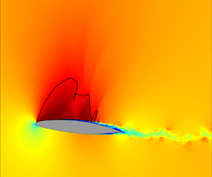
 $\textit {Re} = 5 \times 10^{5}$) was examined for the V2C profile in our previous studies (Zauner et al. Reference Zauner, De Tullio and Sandham2019; Zauner & Sandham Reference Zauner and Sandham2020a,Reference Zauner and Sandhamb). Unlike Dandois et al. (Reference Dandois, Mary and Brion2018), a shock system comprising multiple shock wave structures was observed (identified by where the local Mach number is unity), with the entire shock system exhibiting periodic oscillations. This has been recently confirmed by an ongoing experimental campaign at ONERA (Zauner et al. Reference Zauner, Renou, Dandois, Brion, Moise and Sandham2021).
From this discussion it is evident that further exploration is required in assessing the various models proposed for both laminar and turbulent buffet. In this regard, comprehensive parameter studies for multiple aerofoils are useful for assessing the validity of various models and also for quantifying the sensitivity of buffet to the profile shape. Here, we continue our studies on laminar buffet (Zauner et al. Reference Zauner, De Tullio and Sandham2019; Zauner & Sandham Reference Zauner and Sandham2020a,Reference Zauner and Sandhamb) focusing on Dassault aviation's supercritical laminar V2C profile which complements those on the OALT25 profile carried out by others (Dandois et al. Reference Dandois, Mary and Brion2018; Brion et al. Reference Brion, Dandois, Mayer, Reijasse, Lutz and Jacquin2020). Furthermore, we have opted to employ wall-resolved LES of laminar buffet on the V2C profile, which has several advantages over other methods. Various challenges faced in experimental studies when examining buffet are avoided, including confinement and side-wall effects (Davidson Reference Davidson2016), surface quality/manufacturing tolerances, fluid–structure interaction, measurement uncertainties, wind-tunnel noise and free-stream turbulence levels (Giannelis et al. Reference Giannelis, Vio and Levinski2017). Furthermore, although major insights into buffet features have come from URANS studies (Xiao et al. Reference Xiao, Tsai and Liu2006; Crouch et al. Reference Crouch, Garbaruk, Magidov and Travin2009; Iovnovich & Raveh Reference Iovnovich and Raveh2012, Reference Iovnovich and Raveh2015; Sartor et al. Reference Sartor, Mettot and Sipp2015), these too have several drawbacks related to sensitivity of results to turbulence closure models (Grossi, Braza & Hoarau Reference Grossi, Braza and Hoarau2014; Giannelis et al. Reference Giannelis, Vio and Levinski2017), accuracy of modelling free transition and the capturing of vortex shedding (Grossi et al. Reference Grossi, Braza and Hoarau2014; Sartor et al. Reference Sartor, Mettot and Sipp2015; Poplingher, Raveh & Dowell Reference Poplingher, Raveh and Dowell2019). Indeed, due to the strong sensitivity of predicted buffet features to the turbulence closure model adopted, Giannelis et al. (Reference Giannelis, Vio and Levinski2017) concluded that ‘the simulation of shock buffet through URANS becomes more so an art than a science’, which motivates the present LES study.
In addition to the commonly investigated parameters of  $M$,
$M$,  $\alpha$ and $\textit {Re}$, we also briefly examine the effect of sweep here. Although buffet remains essentially two dimensional (2D) for unswept infinite wings, Iovnovich & Raveh (Reference Iovnovich and Raveh2015) reported three-dimensional (3D) ‘buffet cells’ that occur with the introduction of sweep. Subsequent studies have shown this feature to occur over finite wings (Dandois Reference Dandois2016), arise as a global instability (Crouch et al. Reference Crouch, Garbaruk and Strelets2019; Paladini et al. Reference Paladini, Beneddine, Dandois, Sipp and Robinet2019a; Timme Reference Timme2020) and is related to stall cells superimposed on 2D buffet (Plante et al. Reference Plante, Dandois, Beneddine, Laurendeau and Sipp2020).
The rest of the article is organised as follows. The methodology used for the simulations and modal decomposition are discussed in § 2. A description of the flow states that occur as the different parameters are varied is provided in § 3. Subsequently, the coherent features of these flows are scrutinised in § 4 by performing a spectral proper orthogonal decomposition (SPOD) and reconstructing the flow field based on relevant modes obtained from the same. The implications of these results are discussed in § 5 and § 6 concludes the study.
2. Methodology
2.1. Numerical simulations
2.1.1. Flow solver
The numerical simulations were carried out using the in-house code, SBLI (Yao et al. Reference Yao, Shang, Castagna, Johnstone, Jones, Redford, Sandberg, Sandham, Suponitsky and De Tullio2009), which is a scalable compressible flow solver with multi-block and shock-capturing capabilities and has been used previously to study buffet (Zauner et al. Reference Zauner, De Tullio and Sandham2019; Zauner & Sandham Reference Zauner and Sandham2020a,Reference Zauner and Sandhamb). SBLI solves for the compressible Navier–Stokes equations which govern the flow evolution in a dimensionless form (see Zauner & Sandham Reference Zauner and Sandham2020b, pp. 3–4). The aerofoil chord, the freestream density, streamwise velocity (non-swept) and temperature are used as reference scales implying that their corresponding dimensionless equivalents are given by  $c = \rho _\infty = U_\infty = T_\infty = 1$, respectively. Fourth-order finite difference schemes (central at interior and the Carpenter scheme Carpenter, Nordström & Gottlieb (Reference Carpenter, Nordström and Gottlieb1999) at boundaries) are employed for spatial discretisation, and a low-storage third-order Runge–Kutta scheme is used for time discretisation. To capture features of shock waves, a total variation diminishing scheme is employed, details of which can be found in Sansica (Reference Sansica2015).
2.1.2. LES
To perform the LES, we adopt the spectral-error-based implicit LES approach which has been validated against DNS for flows where buffet is observed (Zauner & Sandham Reference Zauner and Sandham2020b). This approach utilises the error estimator proposed in Jacobs et al. (Reference Jacobs, Zauner, De Tullio, Jammy, Lusher and Sandham2018) for identifying regions of insufficient grid resolution in DNS. Based on this estimator, a low-pass filter is used on all conserved variables to locally correct spectral deviations whenever and wherever they occur. Sixth-order compact finite difference schemes for filtering applications (Lele Reference Lele1992) are used for this purpose. A blending function is used to reduce the impact of filtering at higher wavenumbers. This is given by  $q_{{updated}} = q_{{unfilt.}} - a_{{lim}} (q_{{unfilt.}}- q_{{filt.}})$, where the updated flow field is computed as an affine combination of the unfiltered and filtered flow fields (Bogey & Bailly Reference Bogey and Bailly2004) with the constant, $a_{{lim}} = 0.4$. The parametric values used here are the same as those used in Zauner & Sandham (Reference Zauner and Sandham2020b) (see their table 1).
2.1.3. Geometry, grid and boundary conditions
Dassault Aviation's supercritical, laminar V2C profile with a blunt TE (thickness 0.5 % chord), as used in the TFAST project (Billard et al. Reference Billard2021), is employed in the simulations. To accurately model the blunt TE, maintain grid smoothness and ensure flexibility in the distribution of grid points, C-H multiblock structured grids were generated using an in-house, open-source code (Zauner & Sandham Reference Zauner and Sandham2018). A grid was generated for each incidence angle so as to ensure that the aerofoil wake remains consistently well resolved as  $\alpha$ changes. Features of a typical case of $\alpha = 4^{\circ }$ (‘reference grid’) are highlighted in figure 1(a). The aerofoil (cyan) is treated as an isothermal wall with the temperature set equal to that of the freestream. Integral and zonal characteristic boundary conditions (CBCs) (Sandhu & Sandham Reference Sandhu and Sandham1994; Sandberg & Sandham Reference Sandberg and Sandham2006) are used on the freestream (green) and outflow boundaries (brown), respectively. A localised filter is adopted to handle the singular points at the corners of the blunt TE by employing the strategy proposed in Jones, Sandberg & Sandham (Reference Jones, Sandberg and Sandham2006). For the unswept cases, $x$ and $z$ represent the dimensionless streamwise and spanwise Cartesian coordinates based on the freestream, respectively. The coordinate orthogonal to the two is represented by $y$. The chordwise coordinate is represented by $x'$. The curvilinear circumferential and radial coordinates are $\xi$ and $\eta$, respectively. The 3D grid was obtained by extruding in the $z$-direction with a uniform grid spacing of $10^{-3}$ for two different spanwise lengths, $L_z = 0.05$ (‘narrow domain’) and $L_z = 1$ (‘wide domain’ (WD), see Appendix A.1), with a total of approximately 75 million and 1.5 billion grid points present, respectively. For all cases, the spanwise boundaries are assumed to be periodic (to model an infinite unswept wing). The narrow domain is employed for all cases other than those used to examine the effect of sweep. Note that when $\varLambda = 0^{\circ }$, the flow configuration is of an unswept wing and the $x$-coordinate is based on the streamwise direction. Thus, the freestream $x$-velocity component is unity whereas other components are zero.
Multi-block grid shown by plotting every  $15\mathrm {th}$ grid point in $\xi$ and $\eta$ directions for the case of $\alpha = 4^{\circ }$: (a) entire domain and (b) vicinity of aerofoil. Characteristic boundary conditions (CBCs) are applied on the inflow and outflow boundaries, while isothermal no-slip conditions are applied on the wall. The pink dashed curve is positioned at a normal distance of 0.05 from the aerofoil surface and is used to monitor shock wave features.

The reference grid's features in the aerofoil's vicinity are highlighted in figure 1(b). The blunt TE contains 30 grid points. A curve at a constant wall-normal distance of  $0.05c$ from the aerofoil's surface, is also shown (dashed curve). The latter is used for monitoring shock wave motion and will be referred to as C5 henceforth. The grid clustering is relatively denser close to the aerofoil surface, in its wake, and in the region where the shock wave is expected. The wall-normal and wall-parallel spacings at the wall vary between $1\times 10^{-4}$ to $1.7\times 10^{-4}$ and $4\times 10^{-4}$ to $2\times 10^{-3}$, respectively.
2.1.4. Flow parameters
The fluid is assumed to be a perfect gas with a specific heat ratio,  $\gamma = 1.4$ which satisfies Fourier's law of heat conduction (Prandtl number, $\textit {Pr} = 0.72$). It is also assumed to be Newtonian, with its viscosity variation with temperature governed by the Sutherland's law (Sutherland coefficient, $C_{Suth} = {110.4}/{268.67} \approx 0.41$). We examine the effect of the flow parameters, $M$,
$M$,  $\alpha$, $\textit {Re}$ and $\varLambda$ on buffet by starting from a baseline ‘reference’ case with $M = 0.7$, $\alpha = 4^{\circ }$, $\textit {Re} = 5\times 10^{5}$ and $\varLambda = 0^{\circ }$ and varying the value of only one of these parameters while keeping the other parameters the same as that of the reference. In addition to these, a case at $M = 0.8$ and $\alpha = 0^{\circ }$, with other parameters at reference value, was also simulated to examine buffet features at zero incidence. This is referred to as the A0M8 case (see § 3.2.3). A complete list of all cases studied (except those on grid convergence and domain extent) and the parametric values for each are provided in table 1. Note that the grid resolution close to the leading edge is relatively coarser than at other regions of the aerofoil (figure 1b). This was found to introduce minor grid-level oscillations in the flow field only for the highest incidence angle considered ( $\alpha = 6^{\circ }$, see table 1). This occurred in parts of the buffet cycle when the shock wave moved in close proximity to the leading edge due to the high amplitude of buffet at this $\alpha$. However, this was only during a small part of the buffet cycle and no significant effect on the buffet flow features could be discerned. Nevertheless, higher angles of attack ( $\alpha > 6^{\circ }$) were not examined for this reason. The effect of varying sweep angle, $\varLambda$ is also reported here, but due its limited scope, we present it in Appendix A.
Parameter values for various cases simulated (cases with buffet in boldface).

2.1.5. Temporal features
For all cases except those where  $\alpha$ is varied, the simulations were initialised with freestream conditions used at all grid points. For the study on varying $\alpha$, because it was originally initiated as part of a different study, the initial conditions were chosen as the fully evolved solutions of the reference case. Note that the choice of initial conditions have been shown to not affect flow features that occur past the transients for supercritical aerofoils (Xiao et al. Reference Xiao, Tsai and Liu2006). A constant dimensionless time step of $3.2\times 10^{-5}$ is used (approximately $3\times 10^{5}$ time steps per buffet cycle).
We denote the time taken for the flow to evolve past initial transients as  $t_0$. When oscillations resembling buffet are present in $C_L(t)$ (with $St \sim 0.1$), this approximate transient time, $t_0$, is chosen such that it coincides with the high-lift phase and such that $C_L(t)$ is periodic and the oscillations persist (i.e. do not monotonically dampen) for $t \geqslant t_0$ when visually inspected (e.g. compare figures 2 and 5(a) for the reference case, where $t_0 = 18$). Beyond the transients, the simulations were run until at least 10 low-frequency cycles were completed (or for 20 time units when such oscillations are absent) for the non-swept cases so as to improve statistical convergence of mean quantities and the accuracy of modal decomposition. To confirm if buffet is present, the power spectral density (PSD) of the fluctuating component of the span-averaged lift coefficient, PSD( $C_L'$), was computed based only the data past the initial transient time (i.e. $C_L'(t)$ for $t > t_0$). As the signals are strongly coherent, a periodogram of $C_L'$ was computed with frequency resolution $\delta f \approx 0.01$, sampling frequency, $f_S = 128$ and a Hamming window (to reduce spectral leakage). Through visual inspection, buffet is confirmed to have occurred when there is a time past which $C_L(t)$ exhibits sustained (non-decaying) low-frequency oscillations and when a discernible local maximum is present in the power spectrum in the low-frequency range $0 < St < 0.5$. In addition to the PSD, a continuous wavelet transformation of the same signal ( $C_L'$) was also computed using MATLAB. For this, the commonly used Morse wavelet, with symmetry parameter as 3 and time-bandwidth product as 60, was employed.
Temporal variation of span-averaged aerofoil coefficients, lift, pressure drag, friction drag and TE pressure (corner on suction surface) past initial transients for the reference case. Dashed lines correspond to high-lift (red), low-lift (blue), low-friction-drag (green) and high-friction-drag (brown) phases.

2.2. Validity of simulation results
The LES approach used here is the same as that in Zauner & Sandham (Reference Zauner and Sandham2020b), and has been validated in that study for the reference case by comparing with a DNS. Key flow features, including the frequency and amplitude of buffet agree well between the two. As noted in § 1, an ongoing experimental campaign at ONERA on laminar buffet at Reynolds numbers similar to those studied here has confirmed several results observed in this study including the presence of multiple shock wave structures, shock system oscillation and a buffet frequency of  $St \approx 0.1$ (Zauner et al. Reference Zauner, Renou, Dandois, Brion, Moise and Sandham2021). Further support for the present simulations, including the choice of spanwise width and grid resolution are provided in the following.
2.2.1. Considerations on domain extent
The validation of the LES with DNS in Zauner & Sandham (Reference Zauner and Sandham2020b) was performed in a narrow domain of  $L_z = 0.05$. To examine the effect of spanwise width, an LES for a WD of $L_z = 1$ was also performed. It was observed that some differences exist between the two, including increases in the buffet amplitude ( ${\approx }40\,\%$ difference in PSD of lift fluctuations, compare reference and $\varLambda = 0^{\circ }$ (WD) cases in table 2) and regularity of the oscillations for the WD, but the major flow features, including the development of multiple shock wave structures, their propagation features and buffet frequency (variation of ${\approx }6\,\%$) remain similar.
Mean aerofoil coefficients, separation length and buffet measures for various cases simulated. Here  $St_b$ is the buffet frequency and PSD( $C_L',St_b$) is the PSD of the fluctuating component of lift at $St_b$.

As the focus of this study is on examining qualitative aspects of buffet, we have chosen  $L_z = 0.05$. Results from other previous studies on turbulent buffet also support this choice. Experiments reported in Jacquin et al. (Reference Jacquin, Molton, Deck, Maury and Soulevant2009) have shown that although weak 3D features associated with flow separation are present in the flow, buffet on unswept wings is characterised by a 2D mode. Wall-modelled LES in a domain of span 0.065 $c$ was shown in Fukushima & Kawai (Reference Fukushima and Kawai2018) to accurately capture buffet features observed in experiments. Similarly, in Grossi et al. (Reference Grossi, Braza and Hoarau2014), 3D structures with the spanwise wavelength between $0.029c$ and $0.04c$ were observed in DES.
The flow field in the vicinity of the inflow and outflow boundaries was checked a posteriori for gradients. These were found to be insignificant for all cases simulated. To further investigate the effect of domain extent, a new grid was generated with the domain boundaries extended further by  $40\,\%$. Simulations were carried out for the same settings as $M= 0.85$ and $M = 0.9$. The latter is the case for which the supersonic region's extent was found to be largest, whereas the former is the case for which it is largest and for which buffet occurs (see, e.g., figures 11 and 13). We observed that for $M = 0.85$, the lift coefficient variation and buffet frequency are not significantly different ( $St_b\approx 0.33$, $\bar {C}_L = 0.16$ and the root-mean-square value of $\bar {C}_L' = 0.025$ for both cases) suggesting that for this $M$ and, by extension, for lower $M$ (where supersonic regions are smaller), the effect of extending the domain further on buffet is negligible. For $M = 0.9$, $\bar {C}_L$ was found to increase from 0.35 to 0.39 and the extent of the supersonic region also expanded. Thus, the results of this case alone must be interpreted with caution. However, because the flow remained approximately steady with no buffet present for either domain extent, this case of $M = 0.9$ was not explored further.
2.2.2. Grid resolution
In the present simulations, the main feature of the flow is a laminar BL that develops from the leading edge up to the shock foot. To examine if this is accurately captured, a new grid with 25 % more points was generated ( ${\approx }100$ million grid points), with the grid spacing in $\xi$ and $\eta$ directions in the laminar BL region ( $0 \leqslant x \leqslant 0.5$) approximately halved. The simulation was carried out at the highest Reynolds number studied here ( $\textit {Re} = 1.5\times 10^{6}$). The results, including instantaneous lift coefficient evolution and mean surface coefficients, match well for the two grids (not shown, provided as supplementary material available at https://doi.org/10.1017/jfm.2022.471), confirming the adequacy of the original grid in capturing the laminar BL.
In the regions where the mean flow is attached and turbulent, for most cases studied, the grid spacing in wall units at the aerofoil surface computed based on the mean wall shear stress,  $\Delta \xi ^{+}$, $\Delta \eta ^{+}$ and $\Delta z^{+}$, were found to be approximately 10, 1 and 10, respectively. This indicates that the grid resolution is more than adequate for LES (Garnier & Deck Reference Garnier and Deck2010; Dandois et al. Reference Dandois, Mary and Brion2018). For a few cases close to buffet onset ( $\alpha = 3^{\circ }$ and $M \leqslant 0.69$), the $\Delta \eta ^{+}$ value is higher ( ${\approx }2$), but only in a small region downstream to where shock waves occur (approximately $0.85 \leqslant x \leqslant 0.9$, see figure 6b). Additionally, for $\textit {Re} > 5\times 10^{5}$, we found $\Delta \xi ^{+}$, $\Delta z^{+} \approx 30$ and $\Delta \eta ^{+} \approx 5$ in some regions of the flow. Although the $\Delta \xi ^{+}$ and $\Delta z^{+}$ are still adequate (for comparison, Garnier & Deck (Reference Garnier and Deck2010) used $\Delta \xi ^{+} \approx 50$ and $\Delta z^{+} \approx 20$ for LES), the $\Delta \eta ^{+}$ values are higher than recommended. We do not expect this to play a significant role in affecting buffet dynamics because we have a laminar BL upstream to the shock wave and, downstream, a separation bubble which reattaches only in parts of the buffet cycle to form a turbulent BL which persists only a short distance before reaching the TE. Care has been taken to ensure that the regions associated with separated flow are well-resolved, based on visual checks of instantaneous flow fields and using the spectral-error indicator to check filter activity. In addition, as noted previously, a grid study at $\textit {Re} = 1.5 \times 10^{6}$, did not show any significant changes in buffet features. Thus, the adequacy of the grid is supported by a combination of wall-unit checks, grid sensitivity studies and careful monitoring of simulations using the spectral error detector.
2.3. Modal decomposition and reconstruction
We employ SPOD to examine coherent structures observed in the flow field (Lumley Reference Lumley1970; Glauser, Leib & George Reference Glauser, Leib and George1987; Picard & Delville Reference Picard and Delville2000; Towne, Schmidt & Colonius Reference Towne, Schmidt and Colonius2018). This approach has several advantages over other modal decomposition techniques. Compared with the classic proper orthogonal decomposition, the modes extracted using SPOD are temporally orthogonal and monochromatic. In addition, as compared with the dynamic mode decomposition (DMD), which also obtains modes with such properties, it is shown in Towne et al. (Reference Towne, Schmidt and Colonius2018) that the SPOD modes are optimally averaged DMD modes. Thus, SPOD provides better estimates of coherent features by reducing the ‘noise’ that can accompany DMD modes. This is particularly useful in the modal reconstruction that we have implemented here. Furthermore, the problem of spurious modes that are observed for DMD (Ohmichi, Ishida & Hashimoto Reference Ohmichi, Ishida and Hashimoto2018; Zauner & Sandham Reference Zauner and Sandham2020a) are avoided here. However, note that this approach also suffers from the drawbacks associated with adopting Fourier transforms. For example, temporal variations in frequency can be unresolved (compare with a wavelet transform). In addition, better spectral estimates might require longer simulation times.
2.3.1. Formulation
Given an ensemble of spatiotemporal realisations that represent a stochastic process,  $\{\boldsymbol {q}_\zeta (\boldsymbol {x},t)\}$, with $\zeta$ denoting the realisation's index, a set of orthogonal basis functions, $\{\boldsymbol {\phi }_i(\boldsymbol {x},t)\}$, that ideally represents the coherent aspects of the process is determined by maximising a utility functional (Lumley Reference Lumley1970; Towne et al. Reference Towne, Schmidt and Colonius2018),
 \begin{equation} J(\boldsymbol{\phi}) = E_\zeta\left[\frac{|\langle\boldsymbol{q}_\zeta,\boldsymbol{\phi}\rangle_{(\boldsymbol{x},t)}|^{2}}{ \langle\boldsymbol{\phi},\boldsymbol{\phi}\rangle_{(\boldsymbol{x},t)}}\right]. \end{equation}
Here  $E_\zeta []$ is the expectation operator, and $\langle,\rangle _{(\boldsymbol {x},t)}$ denotes the appropriate inner product over space, $\boldsymbol {x}$, and time, $t$. This allows for choosing each basis function such that the projection of $\boldsymbol {q_\zeta }$ on $\boldsymbol {\phi }_i$, (i.e. $\langle \boldsymbol {q}_\zeta,\boldsymbol {\phi }_i\rangle _{(\boldsymbol {x},t)}$), is maximised over $\zeta$ in a least-square sense. It is possible to show (e.g. by assuming that $\boldsymbol {\phi }_i$ are normal and reformulating using Lagrange multipliers) that the extrema of this functional satisfy the eigenvalue problem
 \begin{equation} \langle {\boldsymbol{\mathsf{C}}}(\boldsymbol{x},\boldsymbol{x}',t,t'),\boldsymbol{\phi}_i(\boldsymbol{x}',t')\rangle_{(\boldsymbol{x}',t')} = \lambda_i\boldsymbol{\phi}_i(\boldsymbol{x},t), \end{equation}
where  ${\boldsymbol{\mathsf{C}}}$ is the two-point spatiotemporal correlation tensor based on any two points $\boldsymbol {x}$ and $\boldsymbol {x}'$ in the spatial domain and $t$ and $t'$ in time, and $\boldsymbol {\phi }_i$ and $\lambda _i$ are the $i$th eigenfunction and eigenvalue, respectively. Note that, as is common for eigenvalue problems, the index $i$ on the right-hand side does not denote a summation. Here, $\lambda _i = J(\boldsymbol \phi _i)$, implying that the maximum of $J$ is given by the maximum eigenvalue. The expansion of any realisation, $\boldsymbol {q}_\zeta$, using the basis $\boldsymbol {\phi }$ is given by
 \begin{equation} \boldsymbol{q}_\zeta(\boldsymbol{x},t) = \sum_i \langle\boldsymbol{q}_\zeta,\boldsymbol{\phi}_i\rangle_{(\boldsymbol{x},t)} \boldsymbol{\phi}_i(\boldsymbol{x},t) = \sum_i a_{i,\zeta} \boldsymbol{\phi}_i(\boldsymbol{x},t), \end{equation}
where  $a_{i,\zeta }$ are the expansion coefficients. It follows from the above equations and the orthonormality of the basis functions ( $\langle \boldsymbol {\phi }_j, \boldsymbol {\phi }_k\rangle _{(\boldsymbol {x},t)} = \delta _{jk}$) that
 \begin{align} E_\zeta[a_{j,\zeta}a_{k,\zeta}^{*}] &= \langle\langle {\boldsymbol{\mathsf{C}}}(\boldsymbol{x},\boldsymbol{x}',t,t'),\boldsymbol{\phi}_j(\boldsymbol{x}',t') \rangle_{(\boldsymbol{x}',t')},\boldsymbol{\phi}_k(\boldsymbol{x},t)\rangle_{(\boldsymbol{x},t)}\nonumber\\ &\Rightarrow E_\zeta[a_{j,\zeta}a_{k,\zeta}^{*}] = \lambda_j \delta_{jk}, \end{align}
where  $\delta _{jk}$ is the Kronecker Delta function and $()^{*}$ denotes complex conjugation.
For a zero-mean, statistically stationary flow, the correlation tensor is dependent only on the time interval,  $\tau = t'-t$ and, thus, a Fourier transform in time can be used to compute the cross-spectral density tensor, ${\boldsymbol{\mathsf{S}}}$. The relations between the two are
 \begin{equation} \left.\begin{gathered} {\boldsymbol{\mathsf{S}}}(\boldsymbol{x},\boldsymbol{x}',f) = \int_{-\infty}^{\infty} {\boldsymbol{\mathsf{C}}}(\boldsymbol{x},\boldsymbol{x}',\tau) \exp({-2\mathrm{i}{\rm \pi} f\tau})\,{\rm d}\tau, \\ {\boldsymbol{\mathsf{C}}}(\boldsymbol{x},\boldsymbol{x}',\tau) = \int_{-\infty}^{\infty} {\boldsymbol{\mathsf{S}}}(\boldsymbol{x},\boldsymbol{x}',f) \exp({2\mathrm{i}{\rm \pi} f\tau})\,{\rm d}f, \end{gathered}\right\}\end{equation}
where  $f$ is the frequency. Following the proof outlined in Towne et al. (Reference Towne, Schmidt and Colonius2018, pp. 859–860), we can relate the eigenvalue problem of ${\boldsymbol{\mathsf{C}}}$ with that of ${\boldsymbol{\mathsf{S}}}$. Assuming the inner product to be a weighted integral in space and time, and substituting for ${\boldsymbol{\mathsf{C}}}$ in (2.5) into (2.2), we get
 \begin{equation} \int_{-\infty}^{\infty}\int_\varOmega\int_{-\infty}^{\infty} {\boldsymbol{\mathsf{S}}}(\boldsymbol{x},\boldsymbol{x}',f) \exp({2\mathrm{i}{\rm \pi} f(t-t')})\,{\rm d}f \,{\boldsymbol{\mathsf{W}}}(\boldsymbol{x}') \boldsymbol{\phi}_i(\boldsymbol{x}',t')\,{{\rm d}\kern0.06em x}'\,{\rm d}t' = \lambda_i\boldsymbol{\phi}_i(\boldsymbol{x},t), \end{equation}
where  ${\boldsymbol{\mathsf{W}}}$ is the weight matrix associated with the quadrature on the curvilinear grid on the spatial domain, $\varOmega$. From the definition of a Fourier transform in time of $\boldsymbol {{\phi }}_i(\boldsymbol {x}',t')$, $\boldsymbol {\hat {\phi }}_i(\boldsymbol {x}',f)$, we obtain
 \begin{align} \int_{-\infty}^{\infty}\int_\varOmega {\boldsymbol{\mathsf{S}}}(\boldsymbol{x},\boldsymbol{x}',f) \,{\boldsymbol{\mathsf{W}}}(\boldsymbol{x}') \hat{\boldsymbol{\phi}}_i(\boldsymbol{x}',f) \exp({2\mathrm{i}{\rm \pi} ft})\,{{\rm d}\kern0.06em x}'\,{\rm d}f = \int_{-\infty}^{\infty} \lambda_i\hat{\boldsymbol{\phi}}_i(\boldsymbol{x},f)\exp({2\mathrm{i}{\rm \pi} ft})\,{\rm d}f. \end{align}
To solve further, we assume the following:
 \begin{equation} \hat{\boldsymbol{\phi}}_i(\boldsymbol{x},f) = \boldsymbol{\psi}_i(\boldsymbol{x},f_0)\delta(f-f_0). \end{equation}
Substituting in (2.7) and eliminating  $\exp {(2\mathrm {i}{\rm \pi} f_0t)}$ on both sides leads to the eigenvalue problem:
 \begin{equation} \int_\varOmega {\boldsymbol{\mathsf{S}}}(\boldsymbol{x},\boldsymbol{x}',f_0) \,{\boldsymbol{\mathsf{W}}}(\boldsymbol{x}') \boldsymbol{{\psi}}_i(\boldsymbol{x}',f_0) \,{{\rm d}\kern0.06em x}' = \lambda_i\boldsymbol{\psi}_i(\boldsymbol{x},f_0). \end{equation}
Here,  $\boldsymbol {\psi }_i(\boldsymbol {x},f_0)$ and $\lambda _i$ are the $i$th eigenfunction and eigenvalue at a given frequency, $f_0$, respectively, with the former referred to as an SPOD mode.
Flow fields were reconstructed using the SPOD mode at a given  $f_0$ by reverting back to the time domain. Using an inverse Fourier transform in time in (2.8), we have
 \begin{equation} \boldsymbol{\phi}_i(\boldsymbol{x},t) = \int_{-\infty}^{\infty} \boldsymbol{\psi}_i(\boldsymbol{x},f_0)\delta(f-f_0)\exp({2\mathrm{i}{\rm \pi} ft})\,{\rm d}f = \boldsymbol{\psi}_i(\boldsymbol{x},f_0) \exp{(2{\rm \pi}\mathrm{i} f_0 t)}. \end{equation}
In addition, although the expansion coefficients,  $a_{i,\zeta }$, vary for different realisations, we are interested in one that best captures the entire ensemble. Based on (2.4), we achieve this by choosing an ideal realisation with an ‘average’ expansion coefficient
 \begin{equation} a_{i,\zeta_0} = \sqrt{E_\zeta\left[|a_{i,\zeta}|^{2}\right]} = \sqrt\lambda_i . \end{equation}
Note that SPOD is carried out after subtracting the mean flow field. Thus, the reconstruction based on the required SPOD mode is obtained by summing up the mean with the real part of the truncated basis expansion. From (2.3), (2.10) and (2.11) we obtain
 \begin{equation} \tilde{\boldsymbol{q}}(\boldsymbol{x},t) = \bar{\boldsymbol{q}}(\boldsymbol{x},t) + \mathrm{Re}\{\sqrt{\lambda_i}\boldsymbol{\psi}_i(\boldsymbol{x},f_0) \exp{(2{\rm \pi}\mathrm{i} f_0 t)}\}, \end{equation}
where  $\tilde {\boldsymbol {q}}$ and $\bar {\boldsymbol {q}}$ represent reconstructed and mean quantities, respectively. This approach is sufficient for the present study, but we note that a more general, low-rank flow reconstruction using SPOD has been implemented for a compressible turbulent jet at a low Mach number in a recently published study (Nekkanti & Schmidt Reference Nekkanti and Schmidt2021).
2.3.2. Implementation
Indexing the eigenvalues such that  $\lambda _1 > \lambda _2 > \lambda _3 > \cdots,$ we have the most-energetic SPOD mode as $\boldsymbol {\psi _1}$ with higher indices representing lower energies. The first two SPOD modes were computed in this study using the memory-efficient streaming algorithm and the software tool provided in Schmidt & Towne (Reference Schmidt and Towne2019). Negligible energy content was observed for $\boldsymbol {\psi _2}$ for all cases studied (comparisons of $\lambda _i$ provided as supplementary material) and thus only features of $\boldsymbol {\psi _1}$ are reported. The weight matrix, ${\boldsymbol{\mathsf{W}}}$, was chosen to represent a weighted 2-norm (see Schmidt & Colonius Reference Schmidt and Colonius2020, § B.2, p. 1027), with its elements being the area associated with each grid point related to the 2D data used for SPOD. The area was approximated as that of the quadrilateral with vertices as the centroids of the cells surrounding a given grid point. SPOD based on an alternative choice of ${\boldsymbol{\mathsf{W}}} = {\boldsymbol{\mathsf{I}}}$ (identity matrix) was also implemented and found to have no significant effect on the qualitative features of the mode shapes or the eigenvalue spectra.
To perform SPOD, two sets of data were used. The first, henceforth referred to as ‘Data-2D’, is based on the instantaneous flow field variables density, velocity vector and pressure, all extracted from the  $z = 0$ plane (no span-averaging). The data based on all these variables at a given time instant were combined together into a ‘snapshot’. Snapshots were stored at regular time intervals of $\Delta t = 0.08$ (sampling frequency, $F_s = 12.5$ implying ${\approx }125$ snapshots per buffet cycle). These were then divided into blocks of total time, $T_\zeta$, each block representing a realisation of the stochastic process. Their number is further increased by using a 50 % overlap and this ensemble is used to compute ${\boldsymbol{\mathsf{S}}}$ using the Welch's method. As noted previously, at least 10 buffet cycles were simulated for all cases where buffet occurs. To examine the low-frequency buffet which occurs at $St \approx 0.1$, it was ensured that at least four cycles occur in a block by choosing $T_\zeta = 44$ (frequency resolution, $\Delta F_\zeta \approx 0.02$). In addition to buffet, we also observed high-frequency coherent structures that we refer to as ‘wake’ modes ( $St \sim O(1$), see figure 23a). To obtain a better spectral estimate of the energy associated with these modes, the number of blocks for SPOD was increased, which reduces the duration associated with each individual block (and, hence, the frequency resolution). For these modes, $T_\zeta = 5$ was chosen, which allows for at least five cycles to be captured while increasing the total number of blocks. As the expected value increases with an increase in the number of realisations in an ensemble, the increase in blocks allows for a better spectral estimate. A higher sampling frequency of $F_s = 125$ was also examined, but no new features were observed in the spectrum.
The second set of data used for SPOD, Data-SpAv, is based on the variation of instantaneous span-averaged wall-pressure and skin-friction coefficients and the local Mach number on the monitor curve C5 shown in figure 1(b). This was only used for flow reconstruction related to a simple one-dimensional representation (in space) of the flow field (e.g., figure 27). The reconstructed  $C_p$ allows to examine the pressure variations on the aerofoil surface, and the reconstructed $C_f$ shows where the flow separates and the reconstructed Mach number giving the approximate position of the shock wave. We found that because the coefficients are span-averaged, this further reduces the non-coherent noise that is present in the SPOD modes. We note that the coherent features extracted are not significantly different between the two approaches and, thus, we have used the second approach exclusively for examining the reconstructed flow field only on the aerofoil surface and the curve C5.
Flow reconstruction based on the desired SPOD mode was carried out based on (2.12). However, because the reconstruction is carried out only at a specified frequency  $f_0$, it is convenient to represent the reconstructed flow based on the phase of the sinusoidal cycle instead of time, $t$. Thus, we use $\phi = 2{\rm \pi} f_0 t$ to compute $\tilde {\boldsymbol {q}}(\boldsymbol {x},\phi )$, with $\phi = 0^{\circ }$ chosen as when the lift coefficient is the maximum.
3. Description of flow states
We first present a basic description of buffet features for the reference case, following which the results for variation of  $M$,
$M$,  $\alpha$ and $\textit {Re}$ are reported (see Appendix A for $\varLambda$). For all cases where buffet occurs, the BL remained laminar up to the vicinity of the shock foot, implying laminar buffet, as categorised in Dandois et al. (Reference Dandois, Mary and Brion2018). A summary of the main results for all cases is provided in table 2. Here, the mean separation length (MSL) on the suction side is computed by summing the lengths of regions where the mean skin-friction coefficient, $\bar {C}_f < 0$. As noted previously, to compute the buffet frequency, $St_b$, the LES was run for at least 10 buffet cycles for the narrow-domain cases and 7 cycles for the $\varLambda = 0^{\circ }$, WD case. For the swept WD cases ( $\varLambda \neq 0$), since only a few cycles were simulated (see Appendix A.1), we do not compute $St_b$. Note that the MSL is not a good representation of the separation dynamics and can be misleading (e.g. compare phase-averaged $C_f$ at high- and low-lift phases in figure 9, Zauner & Sandham Reference Zauner and Sandham2020b). Modal decomposition and flow field reconstruction using modes of interest are considered separately in the subsequent section (§ 4).
3.1. Reference case
Some aspects of the results for the reference case ( $M = 0.7$, $\alpha = 4^{\circ }$, $\textit {Re} = 5\times 10^{5}$ and $\varLambda = 0^{\circ }$) have already been presented in Zauner & Sandham (Reference Zauner and Sandham2020b), but it is useful to review these here to aid later comparisons. The temporal variation of various aerofoil coefficients once buffet has been established are shown in figure 2. Here, $C_L$ and $C_D$ represent the instantaneous span-averaged lift and drag coefficients, with the pressure and skin-friction components of the drag denoted as $(C_D)_p$ and $(C_D)_f$, respectively. Here, the contribution from the blunt TE is neglected when computing the aerodynamic coefficients. The variation of the span-averaged pressure coefficient, $C_p$, at the corner of the blunt TE on the suction surface, $x_{TE}$, is also shown. Low-frequency periodic oscillations (period $\tau _{LES} = 1/St \approx 8.6$ time units) are apparent for all coefficients shown, with the strong fluctuation of the lift coefficient (fluctuation amplitude ${>}10\,\%$ of mean $C_L$) clearly indicating the occurrence of buffet. Minor irregularities between cycles can also be seen, which has been reported for supercritical aerofoils (Roos Reference Roos1980) and at moderate $\textit {Re}$ (McDevitt & Okuno Reference McDevitt and Okuno1985). There are discernible phase differences between all the variables plotted and especially between $C_L$ and $(C_D)_f$. This was observed to be present for all cases simulated here. The time instants when these two coefficients reach their maximum and minimum in a single buffet cycle are highlighted using dashed lines.
To visualise flow features at these times in a manner approximately equivalent to Schlieren images in experiments, contours of streamwise density gradient,  $\textrm {d}\rho /{\textrm {d}\kern0.06em x}$, on the $z = 0$ plane (not span-averaged) are plotted and shown in figure 3. The contour range has been reduced to $[-5,5]$ for clarity while a grey curve is used to delineate the sonic line based on the instantaneous local Mach number, i.e. $M_{{loc}}= 1$. At all times, the presence of multiple shock waves is evident. This appears to be a characteristic flow feature at moderate $\textit {Re}$, as is elaborated in § 3.4. For convenience, we use the term ‘sonic edge’ to refer to the downstream-most edge of the supersonic region, beyond which the flow remains subsonic. In addition, we use the term ‘shock wave structures’ to refer to the multiple shock waves that are present in the flow which are identified by the presence of steep adverse pressure gradients and the sonic line based on the local Mach number, with $M_{loc} = 1$. We observed that the low/high-lift phases of the cycle approximately occur when the sonic edge is at its most upstream/downstream position, respectively, whereas the minimum/maximum $(C_D)_f$ occurs when the sonic edge is approximately at the mid-point of its upstream/downstream motion, respectively.
Streamwise density gradient contours on the  $x\unicode{x2013} y$ plane shown at different phases of the buffet cycle for the reference case: (a) high-lift, (b) low-skin-friction-drag, (c) low-lift and (d) high-skin-friction-drag phases. The sonic line is highlighted using a grey curve.

At  $t = 70$ (figure 3a), when the lift is at a maximum and the sonic edge is at its most downstream position, the shock wave structures appear clustered together at $x \approx 0.6$, and a transitional separation bubble was found to be present for $0.4 \leqslant x \leqslant 0.7$. Subsequently, as the sonic edge moves upstream, the number of shock wave structures reduces and they appear strengthened, while the BL separates and transitions at a more upstream position at $t = 72$ (see $x \approx 0.5$ in figure 3b). When the sonic edge reaches its most upstream position at $t = 74$ (lowest lift, figure 3c), the inclined shock wave structures seem well-separated and the supersonic regions have a triangular shape. The BL reattaches at $x \approx 0.6$, although it remains separated at the TE. At $t = 76$ (figure 3d), at the mid-point of the sonic edge's motion downstream and when $(C_D)_f(t)$ reaches its maximum, the BL remains mostly attached, with a transitional separation bubble present at $0.5 \leqslant x \leqslant 0.7$. A larger supersonic region is present at $t = 70$ and $t = 72$ when compared with $t = 74$ and $t = 76$.
The shock wave motion can be further understood by examining the flow features on the monitor curve C5 highlighted in figure 1b. This curve is at a wall-normal distance of 0.05 from the aerofoil's surface and is above the BL in the supersonic regions of the flow (cf. figure 3). The spatiotemporal variation of the streamwise pressure gradient,  $\textrm {d}p/{\textrm {d}\kern0.06em x}$, on the suction side of this curve is shown in figure 4 (figure 4(b) shows a close-up view of the sonic edge for a single buffet cycle). The contour lines for $M_{loc} = 1$ are overlaid as black curves (sonic line). In determining the sonic edge, we have filtered out the high-frequency variations in the sonic line present in the spatiotemporal diagrams due to the shock wave structures, so that the focus is on the low-frequency buffet. This is shown using a pink dashed curve. Here, the horizontal axis represents the variation in the chordwise direction, whereas the vertical axis represents time. Thus, features with a positive slope represent downstream moving structures and vice versa. The time instants associated with the extrema discussed previously are highlighted using dashed horizontal lines. We emphasise that what is shown are flow features on a single curve at a specified wall-normal distance, so the changes, especially of the sonic line, must be interpreted cautiously.
Spatiotemporal variation of streamwise pressure gradient on the suction side of curve C5 for the reference case: (a) entire suction side and (b) close-up. The approximate times associated with different phases of interest, high lift (red), low skin-friction drag (green), low lift (blue) and high skin-friction drag (brown), are highlighted using dashed lines, and the sonic line and the sonic edge (see the text) are shown using solid black and dashed pink curves, respectively.

The sonic edge (pink dashed curve) is approximately at its most downstream and upstream position at  $t = 70$ (high lift) and 74 (low lift), respectively. Emanating from the sonic edge, we see streaks in the sonic line (black curve) oriented with a negative slope, i.e. propagating upstream. These streaks are due to the shock wave structures and are seen to be only generated during the downstream motion of the sonic edge. These shock wave structures weaken as they travel upstream and eventually seem to degenerate into downstream propagating pressure waves. In the subsonic region downstream of the sonic edge, linear streaks in the pressure gradient contour at a positive slope can be seen (figure 4b). The phase speed of the waves associated with these streaks can be computed from the figure as the inverse of the slope. This falls in the range $0.65\unicode{x2013} 0.7U_\infty$. Lower convection speeds of ${\approx }0.55\unicode{x2013} 0.65 U_\infty$ were observed for other cases studied here. This is similar to the convection speeds, $0.7U_\infty$ and $0.41U_\infty$, of Kelvin–Helmholtz (K–H) instabilities that are reported to accompany buffet in Dandois (Reference Dandois2016) and Dandois et al. (Reference Dandois, Mary and Brion2018), respectively.
The model proposed in Lee (Reference Lee1990) assumes that pressure waves are generated at the shock foot and convect downstream within the BL until they reach the TE (see § 1). Here, the streaks seen in figure 4(b) represent the dominant pressure waves within the BL that reach the TE starting from the sonic edge. The approximate time required for these waves to do so can be inferred from the figure to vary in the range  $0.4 \leqslant t_{down} \leqslant 0.6$ (based on sonic edge's position), which is useful to examine the predictions of Lee's model. This range does not vary significantly when the aerofoil surface is chosen instead of C5, indicating that it is not sensitive to the distance from the aerofoil surface. As shown later in § 4.1, upstream propagating waves outside the BL can be identified using SPOD. The buffet frequency predicted by Lee's model based on these upstream and downstream propagating waves is considered there.
3.2. Effect of Mach number
When the freestream Mach number alone is varied (with  $\alpha = 4^{\circ }$, $\textit {Re} = 5\times 10^{5}$ and $\varLambda = 0^{\circ }$), the lowest value at which a small pocket of supersonic flow develops in the flow field (approximate critical Mach number) was found to be $M = 0.6$. Increasing $M$ further, buffet was observed in the range $0.7 \leqslant M \leqslant 0.85$, above which it was absent. However, for $M \geqslant 0.8$ shock wave structures were observed on both the suction and pressure sides of the aerofoil. Buffet features in the former range are reported first. The cases of higher $M$ are presented subsequently.
3.2.1. Buffet onset and deep buffet
The temporal evolution of  $C_L$ for a few select cases of $M$ in the range $0.5 \leqslant M\leqslant 0.775$ is shown in figure 5(a). For all cases simulated in the range $0.5 \leqslant M \leqslant 0.68$ (see table 1), the variation of $C_L$ is similar to that shown for $M =0.6$ in the figure, with the equilibrium values attained past transients being approximately the same. This occurs even though the flow is entirely subsonic for $M = 0.5$ and becomes transonic at and above the approximate critical Mach number of $M = 0.6$. Interestingly, at $M = 0.69$, sinusoidal oscillations can be discerned during the initial evolution ( $t < 50$), but they slowly dampen with time, with the $C_L$ stabilising at a value close to that of $M = 0.6$. By contrast, a small increase in $M$ to 0.7 (reference case) leads to relatively large-amplitude sustained oscillations implying an abrupt onset of buffet with $M$, which is similar to the results reported for turbulent buffet in Giannelis, Levinski & Vio (Reference Giannelis, Levinski and Vio2018). This trend suggests that a marginally stable eigenmode becomes unstable as the parameter, $M$, is increased from $M=0.69$ to the onset value of $M = 0.7$. This is characteristic of a supercritical Hopf bifurcation and supports the global linear instability model proposed for buffet (Crouch et al. Reference Crouch, Garbaruk and Magidov2007). Interestingly, the maximum of $C_L(t)$ at $M= 0.7$ coincides with that of the approximately steady value attained for pre-onset conditions examined. In addition, a sharp drop in mean lift coefficient past onset is apparent, with $\bar {C}_L$ (the time average of $C_L$) dropping almost linearly with $M$ in a small range of $0.7 \leqslant M \leqslant 0.775$ from approximately 0.85 to $0.3$.
Effect of varying freestream Mach number: (a) temporal variation of lift coefficient and (b) PSD of its fluctuating component as a function of the Strouhal number (for cases for which buffet occurs). The reference case of  $M = 0.7$ is shown using a black curve. Dashed vertical lines and circles highlight the buffet Strouhal number, $St_b$, and peaks in the PSD.

The PSD estimate of the fluctuating component of the lift coefficient,  $C_L'$ is shown in figure 5(b) for cases where buffet is observed. Here, $C_L'(t) = C_L(t)-\bar {C}_L$, where $\bar {C}_L$ is the time-averaged lift coefficient and the PSD is computed using a periodogram of this signal for times after buffet is established ( $t > 18$ for the reference case, see figure 2 and § 2.1.5 for details). The dominant peaks and their corresponding $St$ are highlighted using circles and broken horizontal lines, respectively, with the latter indicating the buffet frequencies, $St_b$. It is evident from the figure that the buffet frequency increases monotonically in the range shown. Such a monotonic increase in frequency with $M$ for turbulent buffet has been previously reported for aerofoils (Dor et al. Reference Dor, Mignosi, Seraudie and Benoit1989; Jacquin et al. Reference Jacquin, Molton, Deck, Maury and Soulevant2009; Giannelis et al. Reference Giannelis, Levinski and Vio2018; Brion et al. Reference Brion, Dandois, Mayer, Reijasse, Lutz and Jacquin2020) and swept wings (Dandois Reference Dandois2016). Note that the buffet frequency seen here is somewhat higher ( $St_b \approx 0.1$, see also table 2) compared with those reported for other commonly used aerofoils (OALT25, OAT15A, NACA0012, for which $0.06 \leqslant St_b \leqslant 0.08$ (Dandois Reference Dandois2016)). However, similar results have been reported for the V2C in simulations (Szubert et al. Reference Szubert, Grossi, Jimenez Garcia, Hoarau, Hunt and Braza2015) and preliminary experiments (Zauner et al. Reference Zauner, Renou, Dandois, Brion, Moise and Sandham2021). For a different supercritical laminar aerofoil, DRA-2303, Hartmann et al. (Reference Hartmann, Klaas and Schröder2012) report a case for which the Strouhal number can be computed to be $St_b = 0.1082$, which is closer to the frequency observed here.
The flow features of pre-onset cases of  $M$ are shown in figure 6 using streamwise density gradient contours. At $M = 0.65$, a small elongated pocket of supersonic region is present. Although there is no shock wave terminating the supersonic region, multiple weak pressure waves can be discerned in the flow at $x \approx 0.5$. Similar ‘wavelets’ were reported in Hilton & Fowler (Reference Hilton and Fowler1947) for low $M$ at which no shock waves were present. In contrast to $M=0.65$, a shock system is observed at $M = 0.69$, with the pressure waves now strengthening sufficiently to form oblique shock waves. As noted previously, we use the term ‘shock wave’ to refer to regions where there are steep adverse pressure gradients (few grid points) within which the local Mach number, $M_{loc}$, becomes unity. By contrast, the term ‘pressure wave’ is used when there are isolated regions of weaker pressure gradients for which $M_{loc}$ is everywhere above or below unity. Thus, shock waves have contours lines of $M_{loc} = 1$ passing through them, whereas pressure waves do not. Note that the time instant shown for $M = 0.69$ is well past the initial transient evolution and after the buffet mode is fully damped (cf. figure 5a). Interestingly, these flow features of $M = 0.69$ resemble those seen for the reference case ( $M = 0.7$) in the high-lift phase (see figure 3a), which is also indicated by the evolution of $C_L$ for these cases.
Streamwise density gradient contours on the  $x\unicode{x2013} y$ plane shown for times well past initial transients for freestream Mach numbers below buffet onset: (a) $M = 0.65$ and (b) $M = 0.69$. The sonic line is highlighted using a grey curve.

Flow features above the onset  $M$ are shown for $M = 0.735$ (top) and $M = 0.75$ (bottom) in figure 7 at high- (left) and low-lift (right) phases of the buffet cycle (see also supplementary movie 1). Note that the maximum PSD( $C_L'$) at buffet frequency is achieved for $M = 0.735$ (cf. figure 5b). For both cases, the flow features far from the aerofoil surface change drastically in a given cycle indicating that buffet can affect the entire supersonic region. Contours of spanwise vorticity magnitude, $|\varOmega _z|$ at these instants are shown in figure 8 for $M = 0.735$. Strongly coherent, concentrated vortices that shed into the wake can be seen in the low-lift phase. Indeed, for all cases where buffet is observed in this study, the vortices were found to be strongest when the sonic edge is at its most upstream position (see also figures 12, 18 and 21). This is also supported by the results based on a time-frequency analysis reported later in § 4.1.1. This contradicts the model proposed in Hartmann et al. (Reference Hartmann, Feldhusen and Schröder2013), which requires that the vortices that reach the TE are most intense when the shock wave is at its most downstream position and vice versa (see their figure 15, p. 14).
Streamwise density gradient contours on the  $x\unicode{x2013} y$ plane shown for the high (a,c) and low (b,d) lift phases of the buffet cycle for the cases $M = 0.735$ (a,b) and 0.75 (c,d). The sonic line is highlighted using a grey curve.

Contours of spanwise vorticity magnitude on the  $x\unicode{x2013} y$ plane shown for (a) high- and (b) low-lift phases of the buffet cycle for the case $M = 0.735$. The sonic line is highlighted using a grey curve.

The spatiotemporal variation of the pressure gradient along the C5 monitor curve is shown in figure 9. Multiple transitions between locally supersonic and subsonic regions that were observed for  $M =0.7$ as the sonic edge moves downstream (figure 4) are reduced here, as indicated by the reduction in the number and extent of the black curves. The approximate times associated with the local extrema of $C_L$ and $(C_D)_f$ are highlighted in the figure using dashed vertical lines (see figure 4 for the colour scheme). As expected, the maximum (minimum) $C_L$ occurs when the sonic edge is at its most downstream (upstream) position. Interestingly, similar to the reference case, the minimum (maximum) $(C_D)_f$ occurs when the sonic edge is approximately in the mid position of its upstream (downstream) motion. Downstream propagating structures in the BL, similar to those seen for the reference case, can also be observed. The convection velocities of these were observed to be slightly lower than in the reference case, with the approximate range of their phase speed being $0.55\unicode{x2013} 0.65U_\infty$, and the time required for them to reach the TE is in the range $0.5 \leqslant t_{down} \leqslant 1.5$ (which is used to comment on Lee's model in § 4.1.2).
Spatiotemporal variation of streamwise pressure gradient on the suction side of C5 for (a)  $M = 0.735$ and (b) $M = 0.75$. The sonic line is highlighted using black curves. The approximate times associated with different phases of interest, high lift (red), low skin-friction drag (green), low lift (blue) and high skin-friction drag (brown), are highlighted using dashed lines.

Mean pressure and skin friction coefficients  $\bar {C}_p$ and $\bar {C}_f$ (computed by time- and span-averaging the flow field) are compared for various $M$ in figure 10. As $M$ increases, we see an increase of $\bar {C}_p$ on the suction surface, and a reduction on the pressure surface. This accounts for the monotonic reduction in mean lift with $M$ seen in figure 5(a). The presence of large-amplitude buffet causes what has been referred to as shock smearing (Giannelis et al. Reference Giannelis, Vio and Levinski2017), where the mean pressure increases along the aerofoil surface in a gradual fashion in contrast to the abrupt increase present when a stationary shock wave occurs (Jacquin et al. Reference Jacquin, Molton, Deck, Maury and Soulevant2009). This can be inferred by comparing the pre-onset cases of $M \leqslant 0.69$ with the rest. From figure 10(b), we see that the mean skin-friction remains approximately a constant on the pressure surface for all $M$, but changes significantly on the suction surface when $M$ is increased above onset. For $M = 0.6$, the presence of a short separation bubble ( $C_f < 0$) can be inferred in $0.64 \leqslant x' \leqslant 0.66$, whereas for $M = 0.69$ and 0.7, there is another region of flow separation seen slightly upstream to this bubble, with the two merging for $M\geqslant 0.735$ to form a separation zone that extends from upstream of the shock foot to close to the TE. Note that although this merged separation zone is present in the mean flow, there are phases in the buffet cycle (high-lift phase) when there is flow reattachment (see § 4).
Variation of mean (time- and span-averaged) (a) pressure and (b) skin friction coefficients along suction (——) and pressure (—  $\cdot$ —) surfaces for various Mach numbers.

3.2.2. High-Mach-number features and buffet offset
For  $M \geqslant 0.8$, shock wave structures are present on both aerofoil surfaces. The temporal variation of $C_L$ for these cases and the PSD of the corresponding fluctuating component are shown in figure 11. The case of $M = 0.775$, for which shock wave structures are observed only on the suction side, is additionally shown for reference. Buffet offset is seen to occur at $M = 0.9$, with $C_L$ approximately a constant, although, as noted in § 2.2.1, the domain extent might not be sufficient and the results must be interpreted with caution. At this $M$ the mean lift is seen to be significantly higher than that of $M = 0.85$. The PSD at the buffet frequency (highlighted using circles) reduces by two orders of magnitude as $M$ is increased from $0.775$ to $0.8$. For $M = 0.8$, low-frequency oscillations are still present, but are accompanied intermittently by high-frequency oscillations of significant amplitude.
(a) Temporal variation of lift coefficient for various freestream Mach number and (b) the PSD of its fluctuating component past initial transient. Dashed vertical lines and circles highlight the buffet Strouhal number and peaks in the PSD. The high-frequency peak ( $St \approx 1.7$) for $M = 0.85$ is highlighted using the square symbol.

The instantaneous flow features at the high- and low-lift phases based on the low-frequency oscillations for  $M = 0.8$ are shown in figure 12. Both the suction and pressure sides have substantial regions of supersonic flow. This development of a supersonic region on the pressure side was observed with increasing $M$ first for $M = 0.775$, with a small ( ${<}0.1c$) pocket of supersonic flow occurring on the pressure side close to mid-chord in part of the buffet cycle, but without any shock wave present. From figures 11 and 12, we can see that although the temporal fluctuations in $C_L$ are low for this $M$, there are significant changes in the sonic edge's positions and the wall-normal extent of the supersonic region. Indeed, the qualitative flow features on the suction side resemble those seen for the other cases where buffet occurs (cf. figure 7).
Streamwise density gradient contours on the  $x\unicode{x2013} y$ plane shown for the (a) high- and (b) low-lift phases of the buffet cycle for $M = 0.8$. The sonic line is highlighted using a grey curve.

For  $M = 0.85$, as shown in figure 11(b), a peak at $St \approx 1.7$ in the PSD is present (highlighted by the square symbol) in addition to that at the buffet frequency. The former arises from a regular vortex shedding and is shown in figure 13(a) at an arbitrary instant. Note that only part of the domain extent is shown. For this $M$, a single shock wave exists at the TE on each aerofoil surface. The shock wave positions on both sides were observed not to change significantly from that shown, although buffet could still be discerned. This was also confirmed using SPOD (not shown). Strongly coherent vortices in the wake, indicating a Kármán vortex street, are apparent from the figure. By contrasting with the reference case, where large-amplitude shock wave motion is observed but the vortical structures are not dominant, we can make an important conclusion that vortex shedding does not directly influence buffet. That is, an increase in vortex shedding strength does not necessarily translate to an increase in buffet amplitude.
Instantaneous streamwise density gradient contours on the  $x\unicode{x2013} y$ plane shown at (a) $M = 0.85$ and (b) $M = 0.9$. The sonic line is highlighted using a grey curve.

The flow features for the offset freestream Mach number,  $M = 0.9$, are shown in figure 13(b). Unlike all the other cases simulated, the BL is now laminar up to the TE, although BL separation still occurs just upstream of the TE on the suction surface. Although quantitative differences exist when the domain is extended (see 2.2.1), these qualitative features were found to be the same. The increase in $C_L$ observed for $M = 0.9$ as compared with $M = 0.85$ (figure 11a) is likely due to this separation being relatively aft for the former. Vortices in the wake are also smaller. Similar results of subdued vortex shedding have been observed when $M$ is increased close to unity for transonic flows over circular cylinders (Murthy & Rose Reference Murthy and Rose1978) whereas the shock wave moving to the TE has been seen for the NACA 0012 aerofoil at zero incidence (Bouhadji & Braza Reference Bouhadji and Braza2003). A fish-tail structure was reported in the latter flow, similar to the one that can be discerned here in the aft of the aerofoil, starting from $x \approx 0.6$.
3.2.3. Buffet at zero incidence on a supercritical aerofoil
Possibly based on distinctions made previously (e.g. Lee (Reference Lee2001, p. 149), ‘There is some difference in the mechanisms of periodic shock motion between a lifting airfoil at incidence and a symmetrical one at zero incidence’ and Iovnovich & Raveh (Reference Iovnovich and Raveh2012, § III, p. 884)), buffet has been classified in Giannelis et al. (Reference Giannelis, Vio and Levinski2017) as either Type I or Type II. The former is typically associated with buffet on biconvex or symmetric aerofoils at zero incidences and is characterised by the presence of shock waves on both aerofoil surfaces. The latter is observed on supercritical aerofoils at relatively high incidence, with shock waves present only on the suction side. Based on the differences in the models for Type I buffet in Gibb (Reference Gibb1988) and Type II buffet in Lee (Reference Lee1990), it was proposed in Lee (Reference Lee2001) that the two types are sustained by distinct mechanisms. This distinction was also noted in Iovnovich & Raveh (Reference Iovnovich and Raveh2012), where the two were referred to as type one and two.
Here, for  $0.7 \leqslant M \leqslant 0.775$, the buffet observed is clearly Type II. However, for $0.8 \leqslant M \leqslant 0.85$, we have buffet with shock waves appearing on both surfaces, albeit at a high incidence angle of $\alpha = 4^{\circ }$. To check if similar buffet features can be observed at zero incidence, we carried out simulations for an additional case of $M = 0.8$ and $\alpha = 0^{\circ }$. The temporal variation of $C_L$ past transients is shown in figure 14, with the reference case result also provided for comparison. The frequency of the oscillations seen was computed as $St \approx 0.14$ for the zero-incidence case, which is slightly higher than that of the reference case ( $St \approx 0.12$), but lower than that of $M = 0.8$ case at $\alpha = 4^{\circ }$ ( $St \approx 0.16$). The mean lift is approximately zero for the zero-incidence case despite the aerofoil not being symmetric (see table 2). The density gradient contours at the high- and low-lift phases are shown in figure 15 (see also supplementary movie 2). The spatiotemporal variations of the streamwise pressure gradient on both the suction and pressure sides of the curve C5 are shown in figure 16. Pockets of supersonic flow and shock wave structures are seen on both surfaces for parts of the buffet cycle, although in other parts of the buffet cycle the flow becomes mostly or entirely subsonic on one of the surfaces. The high-lift (red dashed line) and low-lift (blue dashed line) phases are characterised by the shock wave structures being at their most downstream position on the suction and pressure sides, respectively. Furthermore, the extent of the supersonic regions on either surface varies approximately $180^{\circ }$ out of phase with the other surface which can be inferred by comparing the sonic edge's positions at the high- and low-lift phases in figure 16. This suggests that the present case is of a Type I buffet, albeit on a supercritical aerofoil. This is further explored using SPOD in § 4.3.
Temporal variation of lift coefficient for buffet at zero and non-zero incidence angles.

Streamwise density gradient contours on the  $x\unicode{x2013} y$ plane shown for the (a) high- and (b) low-lift phases of the buffet cycle for $M = 0.8$ at $\alpha = 0^{\circ }$. The sonic line is highlighted using a grey curve.

Spatiotemporal variation of streamwise pressure gradient on the (a) suction and (b) pressure sides of curve C5. The sonic line is highlighted using black curves. The approximate times associated with different phases of interest, high lift (red), low skin-friction drag (green), low lift (blue) and high skin-friction drag (brown), are highlighted using dashed lines.

3.3. Effect of angle of attack
In this section, we examine the effect of incidence angles on buffet. As noted previously, the highest angle reported here is  $\alpha = 6^{\circ }$, although buffet was also observed for $\alpha = 7^{\circ }$, albeit accompanied by minor but persistent grid-level oscillations. At a higher incidence of $\alpha = 8^{\circ }$, preliminary simulations showed that the aerofoil stalls with separation beginning at the leading edge, causing the simulations to fail in the current grid. As the grid requirements for capturing leading edge stall would exceed current computational resources, we were unable to determine whether buffet persists in the presence of stall, although this seems unlikely based on previous studies (Iovnovich & Raveh Reference Iovnovich and Raveh2012; Giannelis et al. Reference Giannelis, Levinski and Vio2018).
The variation of  $C_L$ with $\alpha$ and the PSD of its fluctuating component are shown in figure 17. For $\alpha = 3^{\circ }$, irregular temporal variations are observed, although footprints of buffet can also be discerned. This was confirmed using SPOD (not shown for brevity). For the same flow settings, Zauner & Sandham (Reference Zauner and Sandham2020a) have performed DNS in a wider domain and observed weak buffet indicating onset at this $\alpha$. Based on the observation of Zauner & Sandham (Reference Zauner and Sandham2020b) that a reduction in span can lead to more irregularity in the buffet cycle, we conclude that buffet onset occurs at approximately $\alpha = 3^{\circ }$.
(a) Temporal variation of the lift coefficient past initial transients for various incidence angles and the (b) PSD of its fluctuating component. Dashed vertical lines and circles highlight the buffet Strouhal number and peaks in the PSD.

With increasing  $\alpha$, we see a substantial increase in the amplitude of lift oscillations. The buffet frequency decreases when $\alpha$ is increased from $3^{\circ }$ to $5^{\circ }$, but remains approximately a constant when $\alpha$ is raised to $6^{\circ }$. For turbulent buffet, a similar increase in buffet amplitude is commonly reported (Jacquin et al. Reference Jacquin, Molton, Deck, Maury and Soulevant2009; Giannelis et al. Reference Giannelis, Levinski and Vio2018). However, in contrast to the present results, the frequency is reported to be approximately a constant (Jacquin et al. Reference Jacquin, Molton, Deck, Maury and Soulevant2009) or increase (Dor et al. Reference Dor, Mignosi, Seraudie and Benoit1989; Brion et al. Reference Brion, Dandois, Mayer, Reijasse, Lutz and Jacquin2020) for turbulent buffet.
No qualitative differences in mean aerofoil coefficients ( $\bar {C}_p$ and $\bar {C}_f$) were observed with variations in $\alpha$ and, thus, these results are not shown for brevity. The instantaneous flow features highlight some interesting quantitative differences, as shown in figure 18 using streamwise density gradient contours. For higher $\alpha$, we see a large supersonic region in the high-lift phase (left) which reduces considerably in size in the low-lift phase (right). This is accompanied by a large upstream excursion of the shock structures, which is especially evident for $\alpha = 6^{\circ }$. Similar to cases of buffet at high $M$, large-scale vortices are observed in the low-lift phase.
Streamwise density gradient contours on the  $x\unicode{x2013} y$ plane shown for the (a,c) high- and (b,d) low-lift phases of the buffet cycle for the cases (a,b) $\alpha = 5^{\circ }$ and (c,d) $\alpha = 6^{\circ }$. The sonic line is highlighted using a grey curve.

The spatiotemporal variation of the pressure gradient on the suction side of curve C5 is shown for  $\alpha =5^{\circ }$ and $\alpha =6^{\circ }$ in figure 19. The sonic edge's minimum and maximum position is, as with the other cases, seen to approximately align with the time at which the lift is lowest and highest (horizontal blue and red dashed lines), respectively. However, the motion is no longer symmetrical about the mean position, with the sonic line (black curve) resembling an inverse sawtooth wave at $\alpha = 6^{\circ }$. Based on the slopes observed, we can infer that the sonic edge moves upstream rapidly, whereas its downstream excursion contains phases in which it is substantially slower. The sonic edge moves more rapidly compared with the reference case, which is expected given the strong increase in amplitude, as opposed to the moderate reduction in frequency of the buffet cycle seen at higher $\alpha$ (figure 17b). In addition, the number of shock wave structures is reduced. The time required for the pressure waves to reach the TE was found to be in the range $0.6 \leqslant t_{down} \leqslant 1.1$ (which, as noted previously, is used to comment on Lee's model in § 4.1.2).
Spatiotemporal variation of streamwise pressure gradient on the suction side of C5 for (a)  $\alpha = 5^{\circ }$ and (b) $\alpha = 6^{\circ }$. The sonic line is highlighted using black curves. The approximate times associated with different phases of interest, high lift (red), low skin-friction drag (green), low lift (blue) and high skin-friction drag (brown), are highlighted using dashed lines.

3.4. Effect of Reynolds number
The effect of varying  $\textit {Re}$ is reported here. At the lowest value of $\textit {Re} = 2\times 10^{5}$ simulated, buffet is absent and only BL separation leading to stall was observed. This case is not shown here and we focus only on cases in the range $5\times 10^{5} \leqslant \textit {Re} \leqslant 1.5\times 10^{6}$. One of the motivating factors for this is the presence of multiple shock wave structures at $\textit {Re} = 5\times 10^{5}$. Most other studies, which are usually at higher $\textit {Re}$, report a single shock wave and not the shock system seen here. The temporal variation of $C_L$ and the PSD( $C_L'$) are shown in figure 20. A small reduction of the buffet frequency occurs as $\textit {Re}$ is increased beyond the reference value. Similar minor reduction in frequency has been noted at low $\textit {Re}$ for turbulent buffet (see Raghunathan et al. Reference Raghunathan, Mitchell and Gillan1998; Lee Reference Lee2001). The spectra also show that the first harmonic of the buffet frequency has significant energy content. It is interesting to connect these results with those reported for the V2C using an URANS approach at a higher Reynolds number of $Re \approx 3\times 10^{6}$, at the same $M = 0.7$, in Szubert et al. (Reference Szubert, Asproulias, Grossi, Duvigneau, Hoarau and Braza2016). In the latter study, buffet was not observed at $\alpha = 4^{\circ }$, with onset incidence being predicted as approximately $5.5^{\circ }$. This suggests that if $Re$ is increased with other parameters fixed, there is an offset value of $Re$ beyond which no buffet occurs.
(a) Temporal variation of lift coefficient past initial transients for various freestream Reynolds numbers and (b) the PSD of its fluctuating component. Dashed vertical lines and circles highlight the buffet Strouhal number and peaks in the PSD.

The streamwise density gradient contours for  $\textit {Re} = 1 \times 10^{6}$ and $1.5\times 10^{6}$ are shown in figure 21. It is apparent from the plots that the supersonic-to-subsonic transition is dominated by a single shock wave structure, which is accompanied by only a small pocket of supersonic region downstream. Similar to the other cases, this dominant shock wave structure has an orientation of a negative slope in the low-lift phase. At all times, we observed shock wave structures to be strongly reduced in number in comparison with the reference case, with the supersonic region not having any strong pressure waves (compare with figure 3). This suggests that with further increase in $\textit {Re}$, there could be a critical $\textit {Re}$ above which only a single shock wave is present at all times. This is consistent with other studies on buffet because most of these examine a higher $\textit {Re}$ range than that studied here and report only a single shock wave (e.g. Brion et al. Reference Brion, Dandois, Mayer, Reijasse, Lutz and Jacquin2020).
Streamwise density gradient contours on the  $x\unicode{x2013} y$ plane shown at (a,c) high- and (b,d) low-lift phases of the buffet cycle for the cases (a,b) $\textit {Re} = 1 \times 10^{6}$ and (c,d) $\textit {Re} = 1.5\times 10^{6}$. The sonic line is highlighted using a grey curve.

The spatiotemporal variation of the streamwise pressure gradient at different  $\textit {Re}$ are shown in figure 22. The reduced number of shock wave structures is also apparent here. In addition, these structures are seen to become pressure waves within a short distance from where they first appear, in contrast to the large upstream excursion seen for the other cases at the lower $\textit {Re} = 5\times 10^{5}$ (cf. figures 4, 9 and 19). The time required for pressure waves to propagate from the sonic edge to the TE was found to be in the range $0.5 \leqslant t_{down} \leqslant 0.7$.
Spatiotemporal variation of streamwise pressure gradient on the suction side of C5 for (a)  $\textit {Re} = 1\times 10^{6}$ and (b) $\textit {Re} = 1.5\times 10^{6}$. The sonic line is highlighted using black curves. The approximate times associated with different phases of interest, high lift (red), low skin-friction drag (green), low lift (blue) and high skin-friction drag (brown), are highlighted using dashed lines.

4. Modal decomposition and reconstructed flow fields
The presence of multiple shock wave structures, a turbulent BL and vortices leads to a complex flow field that makes it difficult to understand their individual characteristics. To overcome this issue, we present a modal decomposition using SPOD and study the coherent flow features individually. As will be shown, the two dominant coherent structures are the buffet and wake modes associated with the low-frequency shock oscillations and high-frequency vortex shedding, respectively. A flow field reconstruction based on each of these modes is used to characterise their influence on the dynamics of shock wave BL interactions, which also allows us to examine the different models proposed to explain buffet. For brevity, only the reference case and one case from each parametric variation are reported in the following. Among these, we focus mainly on the former and, in addition,  $\alpha = 6^{\circ }$, for which the buffet amplitude is maximum. The cases where shock waves appear on both aerofoil surfaces are examined separately in § 4.3. Unless otherwise mentioned, the data set used for SPOD is Data-2D (see § 2.3.2).
4.1. Features of modes
4.1.1. Temporal features
A comparison of the spectra for the dominant eigenvalue,  $\lambda _1$, obtained through SPOD for the reference case and one case selected from each parameter variation is shown in figure 23(a). For all cases, we see peaks at a fundamental frequency of $St \approx 0.1$, i.e. the buffet frequency and, in addition, peaks at its harmonics. Significant energy content is also present in a medium-frequency range of $1 \leqslant St \leqslant 4$ associated with what we refer to as wake modes. These are shown in the following to be associated with vortex shedding (e.g. see figure 24c). A bump in the spectrum similar to that seen here and associated with vortex shedding was reported for turbulent buffet in the DES of the OAT15A aerofoil in Grossi et al. (Reference Grossi, Braza and Hoarau2014) and organised eddy simulations of Szubert et al. (Reference Szubert, Grossi, Jimenez Garcia, Hoarau, Hunt and Braza2015). We have also extracted a similar mode at $St \approx 1.87$ for the reference case using DMD in our previous study (Zauner & Sandham Reference Zauner and Sandham2020a). Note that modes similar to the wake modes, and accompanying turbulent buffet, were also reported in Sartor et al. (Reference Sartor, Mettot and Sipp2015). This was shown for the OAT15A using resolvent analysis (see their figures 16 and 18) with a frequency range $0.95 \leqslant St \leqslant 4$ which is the same as the range of $St$ seen here. Although not frequently reported in experiments, Szubert et al. (Reference Szubert, Grossi, Jimenez Garcia, Hoarau, Hunt and Braza2015) have shown that phase-averaging implemented in experiments to capture buffet features can prevent the effects of such modes from being observed. From the figure, it is evident that a change in any parameter ( $M/\alpha /\textit {Re}$) leads to an increase in the energy content of the wake modes, indicating a stronger vortex shedding beyond buffet onset. With increasing $\alpha$, the frequency associated with these modes seems to be shifted to lower values.
(a) Eigenvalue spectra (logarithmic scale) based on SPOD of the dominant eigenvalue for the reference case and a typical case for each parameter varied. Circles highlight the buffet peaks. (b) Scalogram based on the lift coefficient ( $\log _{10} |W(C_L')|$) with the temporal variation of the same overlaid (black curve) for the case of $\alpha = 6^{\circ }$.

SPOD modes for the reference case shown using contour plots of real part of the density field: (a) buffet mode ( $St = 0.11$), (b) its first harmonic ( $St = 0.23$) and (c) a wake mode ( $St = 2.1$). The red, black and blue curves represent the sonic lines based on the high-lift phase, mean flow and low-lift phase, respectively.

To check for temporal variations in the intensities and frequencies of these modes, a time-frequency analysis using the continuous wavelet transform was also carried out (see § 2.1.5 for details). The scalogram based on the transform of the lift coefficient's fluctuating component,  $W(C_L')$, is shown for the case of $\alpha = 6^{\circ }$ in figure 23(b). Note that the contours are based on the logarithm of the magnitude, i.e. $\log _{10} |W(C_L')|$. The temporal variation of $C_L$ is also overlaid to identify high- and low-lift phases. A horizontal band in the contour at the buffet frequency ( $St \approx 0.1$) confirms that it does not vary with time. However, it is also evident that there are periodic changes of $|W(C_L')|$ in the frequency range $1 \leqslant St \leqslant 3$. As seen from figure 23(a), this is associated with the wake modes for this case. It is evident from the figure that the intensity of these modes is approximately a maximum in the low-lift phase and vice versa. This is expected based on the vortex shedding behaviour reported in § 3.3 (see figure 18). Similar results have been reported for turbulent buffet in Szubert et al. (Reference Szubert, Grossi, Jimenez Garcia, Hoarau, Hunt and Braza2015).
4.1.2. Spatial features
The spatial structure of the SPOD modes of importance are shown for the reference case in figure 24 using the real part of the density field. From left to right, these are the buffet mode ( $St = 0.11$), its first harmonic ( $St = 0.23$) and a typical wake mode ( $St = 2.1$), where the bump in the spectra attains a local maximum). The sonic line based on the mean local Mach number (black curve) is shown for reference along with the sonic lines at high- (red) and low-lift (blue) phases (reconstructions, see § 4.2.1). For the buffet mode we see that strong density fluctuations are present in the vicinity of the TE and near-wake which are out of phase (i.e. opposite sign) with those near the shock foot. Thus, the density increases at the shock foot when it reduces at the TE and in the wake and vice versa. The harmonic mode is of a shorter wavelength relative to the buffet mode. The mode shapes of the buffet mode and its harmonic reported here are similar to those in Poplingher et al. (Reference Poplingher, Raveh and Dowell2019) for turbulent buffet (see their figure 9).
The wake mode has a structure similar to that of the von Kármán vortex street. Similar structures were also observed in the resolvent analysis of steady RANS solutions in Sartor et al. (Reference Sartor, Mettot and Sipp2015) where they are referred to arise as Kelvin–Helmholtz instabilities. Note that the flow field contains both a free shear layer due to a separated BL and a wake. The former can lead to a Kelvin–Helmholtz inflectional instability. On the other hand, a von Kármán instability can arise in the wake and studies such as Triantafyllou & Karniadakis (Reference Triantafyllou and Karniadakis1990) and Pier & Huerre (Reference Pier and Huerre2001) have shown that this instability can arise even when only the wake is considered in isolation (i.e. without the inclusion of the solid body and upstream regions). Although the wake mode's structure resembles a von Kármán vortex street (see also figure 8), a stability analysis is required to understand the origin of the instability that leads to this mode which is beyond the scope of this study.
In addition to this, waves in the flow field that seem to be generated at the TE and propagate upstream outside the BL on both sides of the aerofoil can be identified. These appear to be the Kutta waves suggested in Lee (Reference Lee1990). Based on visualisations of the time evolution of the wake mode, the upper limit on the time required for these waves to reach the shock wave starting from the TE was estimated as  $t_{up} < 1.5$. Thus, for the reference case, Lee's model predicts the buffet time period as $\tau _{Lee} = t_{up}+t_{down} < 2.1$, which is substantially lower than the actual buffet period of $\tau _{LES} =8$ observed in the LES (see § 3.1). Similar results were observed for other wake modes associated with the spectral bump and for all other cases where buffet was observed, suggesting that Lee's model is invalid. This is further considered in § 5.3.
The modification to Lee's model proposed in Jacquin et al. (Reference Jacquin, Molton, Deck, Maury and Soulevant2009) assumes that  $t_{up}$ should be replaced with $t^{J}_{up}$, the time required for the waves to travel upstream along the pressure surface and turn around the leading edge to reach the shock foot. Such upward propagating waves are also seen in figure 24(c) on the pressure side of the aerofoil. However, we observed that they reduce in intensity by more than an order of magnitude upstream of mid chord and they are unidentifiable past the leading edge in the supersonic region, likely because their intensity is reduced to levels similar to that of noise in the SPOD modes. By using the same approximation as Jacquin et al. (Reference Jacquin, Molton, Deck, Maury and Soulevant2009) that the time spent in the supersonic region is negligible, we observed $t^{J}_{up} < 3$ implying that the predicted time period is $\tau _J = t^{J}_{up}+t_{down} < 3.6$ which still remains significantly lower than $\tau _{LES}$.
Features of the corresponding SPOD modes for  $\alpha = 6^{\circ }$ are shown in figure 25. We see that the wave number associated with each mode is substantially lower with all modes showing a larger spatial structure. A relatively strong separation in the vicinity of the shock foot is apparent, whereas the wake mode's energy is high at the TE. These results match with the flow features observed in the simulations (cf. figures 3 and 18). Similar to the reference case, upstream propagating waves emanating from the TE can be observed for the wake mode. Based on this, it was estimated that $t_{up} < 2$ and $t^{J}_{up} < 3$ implying that $\tau _{Lee} < 3.1$ and $\tau _J < 4.1$ compared with $\tau _{LES} = 9.9$.
SPOD modes for  $\alpha = 6^{\circ }$ shown using contour plots of real part of the density field: (a) buffet mode ( $St = 0.10$), (b) its first harmonic ( $St = 0.21$) and (c) a wake mode ( $St = 1.3$). The red, black and blue curves represent the sonic lines based on the high-lift phase, mean flow and low-lift phase, respectively.

4.2. Modal reconstruction
The features of the buffet and wake modes are further scrutinised here by performing a flow field reconstruction, superposing each mode separately with the mean flow field. All quantities described here (lift, velocity, local Mach number, etc.) are based on the reconstructed flow field. As noted in § 2.3.2, the temporal variation is described using the phase,  $\phi$, with $\phi = 0^{\circ }$ and $180^{\circ }$ signifying the phases at which maximum and minimum lift (reconstructed) are attained, respectively.
4.2.1. Buffet mode
Contours of axial velocity at different phases are shown in figure 26 for  $\alpha = 6^{\circ }$. For this case, the phases of $\phi = 73^{\circ }$ and $253^{\circ }$ represent the minimum and maximum skin friction drag, respectively. In contrast to the actual flow field in which multiple shock structures are present, the reconstructed flow field contains only a single supersonic region enclosed by the sonic line. This is expected, because these multiple shock structures arise at a frequency higher than the buffet frequency (see, e.g., figure 4). For convenience, the approximate aft part of the sonic line that terminates the supersonic region is referred to as a shock wave. The BL remains attached over most of the aerofoil when the shock wave is at its most downstream position ( $\phi = 0^{\circ }$). As the shock wave moves upstream, we see that at $\phi = 73^{\circ }$, the flow is fully separated beyond the foot of the shock wave ( $\tilde {u}_x < 0$). As the shock wave reaches its most upstream position ( $\phi = 180^{\circ }$), the BL is attached until $x \approx 0.7$. We found the qualitative features described previously to be common to all cases considered.
Reconstructed flow field based on the buffet mode for  $\alpha = 6^{\circ }$ shown using axial velocity contour at (a) high-lift, (b) low-skin-friction-drag, (c) low-lift and (d) high-skin-friction-drag phases. The sonic line is highlighted using a black curve.

To better understand the dynamical behaviour of buffet, it is useful to examine the variation of flow features on the aerofoil surface at different phases. This spatiotemporal variation is reconstructed based on the data set Data-SpAv (see § 2.3.2) and shown using  $x'-\phi$ diagrams for the different cases in figure 27 (right-hand side contours). Unlike the preceding sections where the streamwise pressure gradient on the curve C5 was used to scrutinise shock wave structures, we show here the variation of the pressure coefficient on the aerofoil surface. In addition, we overlay the contour line, $\tilde {C}_f = 0$ (green curve), which delineates flow reversal ( $\tilde {C}_f \leqslant 0$). To include the shock wave position, we also overlay the sonic line based on the local Mach number (black curve). We emphasise that only this quantity is computed based on the curve C5 whereas the rest are based on the aerofoil surface. As before, the phases at which minimum and maximum $(\tilde {C}_D)_f$ occur are highlighted using dashed horizontal lines.
Temporal variation of the shock wave's strength shown using  $\tilde {M}_{eff}$ (left-hand side subplot) and spatiotemporal contours of $\tilde {C}_p$ on the aerofoil suction surface (right-hand side contours) for (a) reference, (b) $M = 0.735$, (c) $\alpha = 6^{\circ }$ and (d) $\textit {Re} = 1.5\times 10^{6}$ cases. The isolines for $\tilde {M}_{loc} = 1$ (solid black curve) and $\tilde {C}_f = 0$ (solid green curve) and the phases associated with maximum (dashed brown line) and minimum (dashed green line) $(\tilde {C}_D)_f$ are also shown for reference.

The shock wave's most upstream and downstream positions (black curve) occur when the lift is close to its minimum ( $\phi = 180^{\circ }$) and maximum ( $\phi = 0^{\circ }$), although there seems to be a small phase lag between the two. As alluded to in § 3.1, the maximum and minimum $(\tilde {C}_D)_f$ occur when the flow is ‘least’ and ‘most’ separated, as can be inferred from the chordwise extent of separation delineated by the $\tilde {C}_f = 0$ isoline (green curve). Indeed, the BL remains separated up to the TE ( $\tilde {C}_f < 0$) at the phase when the minimum $(\tilde {C}_D)_f$ is attained (dashed horizontal green line) for all cases. By contrast, during the phase of maximum $(\tilde {C}_D)_f$ (dashed horizontal brown line), the BL is fully attached from the leading edge to TE for the cases $\textit {Re} = 1.5\times 10^{6}$ and $\alpha = 6^{\circ }$, whereas the flow reattaches ( $\tilde {C}_f > 0$) downstream to the shock wave (black curve) and remains attached up to the TE for the other cases. Thus, we can conclude that the surface coefficients $\tilde {C}_L$ and $(\tilde {C}_D)_f$ are approximate indicators of the shock wave position and the BL separation, respectively. The reasons for these relations can be explained by observing that a negative $\tilde {C}_p$ exists upstream of the shock wave, and an increase in the chordwise extent of this low-pressure region leads to an increased lift. Similarly, as mentioned previously, an attached BL leads to larger skin friction due to large positive velocity gradients on the aerofoil surface, whereas a separated BL and flow reversal above the surface contribute to a low $(\tilde {C}_D)_f$.
Another aspect of interest is the temporal variation of the shock wave's strength as it is expected to play an important role in BL separation and, thus, on buffet. One estimate of this strength is the ratio of the instantaneous pressure immediately downstream and upstream of the sonic line in the  $x-\phi$ diagram, $\tilde {p}(x^{+}_S,\phi )/\tilde {p}(x^{-}_S,\phi )$, where $x_S$ represents the shock wave's streamwise position (i.e. $x_S = x(\tilde {M}_{loc} = 1)$) and the symbols ‘ $+$’ and ‘ $-$’ indicate downstream and upstream, respectively. However, this choice was found to be sensitive to the choice of $x^{+}_S$ and $x^{-}_S$. This is possibly because the actual flow field has multiple shock wave structures and the single shock wave seen in the modal reconstruction is only an approximation, implying that choosing points both upstream and downstream of the shock introduces relatively large errors in the estimation of the pressure ratio. Instead, we found the upstream effective Mach number, which is based on the instantaneous upstream velocity in the inertial frame of reference moving at a speed equal to the instantaneous speed of the shock wave (i.e. $\textrm {d}\kern0.06em x_S/\textrm {d}\phi$), to be more robust with regard to the choice of $x^{-}_S$. This is given by
 \begin{equation} \tilde{M}_{eff}(x^{-}_S,\phi) = \tilde{M}_{loc}(x^{-}_S,\phi) - \left(\frac{{\rm d}\kern0.06em x_S}{{\rm d}t}\right)\frac{1}{a(x^{-}_S)}, \end{equation}
where  $a$ represents the local speed of sound. The effective Mach number can then be used to represent the shock strength based on the Rankine–Hugoniot conditions (Gibb Reference Gibb1988). However, note that this approximation neglects the effect of shock wave acceleration. The left-hand side subplots in figure 27 show the effective upstream Mach number's temporal variation for $x_S^{-} = x_S - 0.1$. It is seen from the plots that $\tilde {M}_{eff}$ reaches a maximum or minimum when the shock is approximately at the mid-point of its upstream or downstream excursion, respectively. This implies that the shock wave is always strongest/weakest close to its mean streamwise position during its upstream/downstream motion. A similar result based on Mach number was shown in Fukushima & Kawai (Reference Fukushima and Kawai2018) (their figure 18), and other studies have also noted the same trend (Tijdeman & Seebass Reference Tijdeman and Seebass1980; Lee Reference Lee2001; Iovnovich & Raveh Reference Iovnovich and Raveh2012; Hartmann et al. Reference Hartmann, Feldhusen and Schröder2013). The plots show that there is a small interval in which $\tilde {M}_{eff} < 1$. This is possibly not of physical significance, because there are shock wave structures present at all times suggesting that it arises due to the approximations in the estimate of shock strength.
From figure 27, the following sequence of events can be inferred for all cases.
(i) When the shock wave is at its most downstream position, the BL is separated upstream of the shock wave, but reattaches downstream, forming a separation bubble.
(ii) As the shock moves towards the leading edge, it strengthens. The upstream separation point moves in the same direction and the reattachment point moves further downstream (or vanishes), increasing the chordwise extent of the separation region.
(iii) The BL is ‘most’ separated when the shock wave is approximately at the mid-point of its upstream excursion, where its strength is close to its maximum.
(iv) Past the mid-point, the BL separation weakens leading to the formation of a separation bubble that reattaches at the shock foot for all cases except $M = 0.735$, where this occurs later.
(v) Once the shock wave reaches its most upstream position and starts to move downstream, the separation point upstream of the shock wave abruptly moves downstream by almost
$\delta x' = 0.1$ for the $M = 0.735$ and reference case, whereas it completely vanishes for the other cases.(vi) As the shock wave reaches the midpoint of its downstream excursion it strength is relatively weakened and the flow is ‘least’ separated.
(vii) The reattached flow is associated with a pressure rise in the TE region, with this back pressure exceeding the freestream pressure (red contours,
$\tilde {C}_p > 0 \Rightarrow \tilde {p} > \tilde {p}_\infty$). The chordwise extent of this region of increased pressure attains a maximum before the shock wave reaches its most downstream position.


The above description indicates that the laminar buffet observed in this study is essentially related to a moving shock wave of temporally varying strength whose motion is accompanied by BL separation and reattachment. Importantly, the following two features are common to all buffet cases studied: a phase lag between the shock wave position and the separation extent and the build up of back pressure. In addition, it is interesting to note that, for all cases, there are phases in the buffet cycle where the flow separation extends up to the TE, indicating that the aerofoil is intermittently stalled. However, we emphasise that it is difficult to disentangle cause, correlation and effect. The possible implications of these observations are discussed in § 5.
4.2.2. Wake mode
The contours of reconstructed axial velocity field based on the wake mode for the case of  $\alpha = 6^{\circ }$ are shown in figure 28 at phases corresponding to the highest ( $\phi = 0^{\circ }$) and lowest ( $\phi = 180^{\circ }$) values of $\tilde {C}_L$. Note that the phase, $\phi$, considered here is based on the time period of the wake mode and not the buffet mode. Thus, the high-lift phase signifies the phase at which the wake mode interaction with the mean flow induces the maximum lift obtained for the reconstructed flow field and is not related to the buffet mode. In the plots, the sonic line (black curve) indicates that the shock foot extends and retracts at different phases, similar to the shock foot motion observed in Dandois et al. (Reference Dandois, Mary and Brion2018) for the OALT25 at $M = 0.735$, $\alpha = 4^{\circ }$ and $Re = 3\times 10^{6}$, implications of which are discussed in § 5.1. The streamwise positions of the sonic edge at $\phi = 0^{\circ }$ and $180^{\circ }$ are $x \approx 0.6$ and 0.5, respectively, implying that the shock foot moves approximately a streamwise distance of 10 % chord. This indicates that the wake mode can cause significant variations in the flow field. However, these are limited to the shock foot as the approximate wall-normal height up to which differences in the sonic line at these two phases are significant is only around 10 % (contrast with figures 26(a) and 26(c) for the reconstruction based on the buffet mode, where the streamwise distance moved is 30 % chord with the sonic line changing drastically in the wall-normal direction also).
Reconstructed flow field based on the wake mode for  $\alpha = 6^{\circ }$ shown using axial velocity contour at (a) high- and (b) low-lift phases. The sonic line is highlighted using a black curve.

4.3. High-Mach-number features
The spatial structure of the buffet mode, its first harmonic and a typical wake mode for the A0M8 case ( $\alpha = 0^{\circ }$ and $M = 0.8$) are shown in figure 29 using the real part of the density field. It is evident that the buffet mode is approximately antisymmetric about the $y$-axis, which indicates that the flow behaviours on the suction and pressure sides are out of phase with each other. By contrast, the first harmonic exhibits symmetric features.
SPOD modes for the A0M8 case ( $\alpha = 0^{\circ }$, $M=0.8$) are shown using contour plots of the real part of the density field: (a) buffet mode ( $St = 0.13$), (b) its first harmonic ( $St = 0.27$) and (c) a wake mode ( $St = 1.86$). The red, black and blue curves represent the sonic lines based on the high-lift phase, mean flow and low-lift phase, respectively.

Reconstructions using the data set Data-SpAv and based on the buffet mode at  $M = 0.8$ for the cases of $\alpha = 0^{\circ }$ (A0M8 case) and $\alpha = 4^{\circ }$ ( $M=0.8$ case) are shown in figure 30. The effective Mach number is not plotted here because there are phases at which no shock wave is present for the case of $\alpha = 0^{\circ }$ on the pressure side. It is evident from the figure that the motion of shock wave (black curve) on the suction side is of similar amplitude as that observed for other $M$ (cf. figure 27). However, the flow is also seen to be separated downstream of some chordwise position for almost all times, especially at $\alpha = 4^{\circ }$. Importantly, this implies that strong buffet can occur even when the BL is permanently separated. Note also that for the $M = 0.8$ and $\alpha = 4^{\circ }$ case, the amplitudes of lift fluctuations are relatively low as compared with lower $M$ (see figure 11b), although the amplitude of shock wave motion remains approximately the same. This implies that the determination of buffet occurrence merely based on temporal variations in $C_L$ or $C_p$ might not be always accurate due to the low variation in these coefficients when the BL is permanently separated.
Spatiotemporal contours of  $\tilde {C}_p$ for the cases of (a,b) $\alpha = 0^{\circ }$ and (c,d) $\alpha = 4^{\circ }$ at $M = 0.8$ on (a,c) suction and (b,d) pressure surfaces. The isolines for $\tilde {M}_{loc} = 1$ (solid black curve) and $\tilde {C}_f = 0$ (solid green curve) and the phases associated with maximum (dashed brown line) and minimum (dashed green line) $(\tilde {C}_D)_f$ are also shown for reference.

As noted before, a phase difference between the shock wave positions on the suction and pressure sides is present for both cases. For  $\alpha = 4^{\circ }$, although the amplitude of the streamwise excursion of the shock wave on the pressure side is relatively weak in comparison with that on the suction side, the former was found to lag the latter by ${\approx }69^{\circ }$. For the $\alpha = 0^{\circ }$ case, in which the shock wave vanishes for part of the cycle, this phase difference was computed using the most downstream shock position. This was computed as approximately $179^{\circ }$, which is similar to that seen for biconvex aerofoils (McDevitt et al. Reference McDevitt, Levy and Deiwert1976). A phase difference between the shock wave positions and the extent of flow separation is also seen in figure 30, albeit, significantly reduced. An increase in back pressure close to when the shock wave reaches its most downstream position can also be discerned. Thus, these two features seem to be common to all buffet cases simulated here.
5. Discussion
5.1. The relation between laminar and turbulent buffet
An important conclusion on the relation of laminar and turbulent buffet can be made based on the present results. Laminar buffet, as identified in Dandois et al. (Reference Dandois, Mary and Brion2018), is characterised by the BL remaining laminar up to the shock foot during the entire buffet cycle. Based on their simulations of the OALT25 at a specific flow setting, the authors concluded that unlike the turbulent buffet, which occurs as a ‘global instability of the flow with intermittent boundary-layer separation and reattachment between the shock and the trailing edge’, the laminar buffet occurs due to a ‘separation bubble breathing phenomenon associated with a vortex shedding mechanism’. In the present study, the previous sections clearly show that we have a laminar buffet, with the BL laminar until the vicinity of the shock foot for all cases studied (e.g. figure 3). However, the results of the SPOD reconstruction of the buffet mode indicate that the laminar buffet observed here is driven by boundary-layer separation and reattachment (see figure 27), a characteristic feature of turbulent buffet.
The modal reconstruction based on the wake mode shows that this mode can cause a localised motion of the shock foot (figure 28), and the vortices shed are characteristic of bubble breathing observed in shock wave BL interactions. Thus, we suggest that the self-sustained oscillations reported in Dandois et al. (Reference Dandois, Mary and Brion2018) are not associated with the buffet mode, but are due to the wake mode. These two modes can both coexist for the same flow settings, as shown here for the V2C and it is possible that for the OALT25, the wake mode alone is the predominant unstable mode under certain conditions, and the buffet mode is weak. This hypothesis is supported by the experimental results for the same aerofoil reported in Brion et al. (Reference Brion, Dandois, Mayer, Reijasse, Lutz and Jacquin2020), where an increase in  $\alpha$ or $M$ at $\textit {Re} = 3\times 10^{6}$ leads to the emergence of a minor low-frequency peak at $St \approx 0.05$. This peak can be interpreted as indicating weak laminar buffet occurring in the experiments (in contrast to the strong dominant discrete peak at $St\approx 0.1$ seen here). This interpretation is supported by some interesting differences that exist between the experimental and LES results. As noted in § 3.4, buffet offset can occur with increasing $Re$, suggesting that the experiments might be close to offset conditions at the higher $Re \approx 3\times 10^{6}$ studied there. Similarly, because shock wave position strongly affects the strength of vortices shed (see, e.g., figures 7 and 23b), this would explain the broad frequency range associated with the wake modes seen here ( $1 \leqslant St \leqslant 4$) compared with the discrete frequency peak at $St \sim O(1)$ seen in the experiments.
Based on these considerations, we conclude that laminar buffet is essentially the same as turbulent buffet with regard to the physical mechanisms that sustain the low-frequency oscillation. This allows for using the present results to make general comments on the buffet phenomenon. Note that quantitative differences (e.g. onset conditions and buffet amplitude) between the laminar and turbulent buffet types are expected due to features such as the laminar/turbulent BL's streamwise variation of thickness and tendency to separate.
5.2. The relation between Type I and II buffet
In the previous sections, we have shown that buffet also occurs at zero incidence ( $M = 0.8$ and $Re = 5\times 10^{5}$) with shock waves present on both aerofoil surfaces exhibiting oscillatory motion such that they are out of phase with each other. These aspects are the defining characteristics of Type I buffet, albeit for a supercritical aerofoil instead of a biconvex/symmetrical aerofoil as is typically reported. However, the flow features seen for this case, including the presence of multiple shock wave structures and the temporal variation of $C_L$, also resemble those observed for Type II buffet discussed for $0.7 \leqslant M \leqslant 0.775$ at $\alpha = 4^{\circ }$. This indicates that Type I and Type II buffet potentially have the same underlying mechanisms. Similar inferences can also be made from McDevitt & Okuno (Reference McDevitt and Okuno1985) for the symmetric NACA 0012 aerofoil (see their figure 25) and it would be interesting to see whether this can be confirmed further by looking for Type I buffet on other commonly used supercritical aerofoils. Thus, although it is still useful to differentiate buffet into these two types to highlight the presence or absence of shock waves on the pressure side, the two appear to be governed by the same mechanisms irrespective of the aerofoil used. This implies that any model for buffet should be capable of explaining either buffet type.
Building on earlier studies (Tijdeman Reference Tijdeman1977; McDevitt & Okuno Reference McDevitt and Okuno1985), Gibb (Reference Gibb1988) proposed a model for Type I buffet based on an instability arising from the shock wave BL interactions which couples with the wake deflection, i.e. if a perturbation causes the shock wave on one side, say the upper surface, to move upstream, it can cause it to strengthen leading the BL to separate at its foot which would cause the wake to deflect upward. This would cause the flow on the lower surface to accelerate, causing the shock wave on that surface to move downstream further deflecting the wake upward which, in turn, promotes the upstream excursion of the upper shock wave. This would continue until the upper shock wave moves sufficiently far upstream that the local Mach number it encounters is small, causing it to weaken, which, in turn, leads to BL reattachment and subsequent downstream motion. This model requires that shock waves are present on both aerofoil surfaces and play an active role in sustaining buffet. However, this model fails for Type II buffet, where there is a negligible temporal variation in the coherent flow features on the pressure side (see, e.g., pressure side, figure 26). Similarly, models proposed exclusively for Type II buffet must be reinterpreted to explain Type I buffet.
5.3. The wake mode and the model of Lee
As shown in § 4.1, the time periods of buffet predicted by the models proposed in Lee (Reference Lee1990) and Jacquin et al. (Reference Jacquin, Molton, Deck, Maury and Soulevant2009) are substantially lower than those observed in the simulations. Although this quantitative difference implies that the models are inaccurate, there are physical reasons to suspect that the proposed physical mechanism itself is invalid. As indicated by the results of SPOD, the waves that are observed in these simulations are due to the wake modes. These modes are essentially related to vortex shedding implying that they are primarily dependent on the position of the BL separation. Although the buffet mode strongly influences BL separation, the results from the variation of  $M$ indicate that the buffet mode is not influenced by the intensity of vortex shedding. First, wave propagation can be discerned for cases where no buffet is present, as seen for the case $M =0.65$ (figure 6a). In addition, as $M$ is increased from $M = 0.7$ to 0.85, we observe a monotonic increase in vortex shedding intensity, but the energy of the buffet mode initially increases when $0.7 \leqslant M \leqslant 0.735$ and substantially reduces when $0.735 \leqslant M \leqslant 0.85$. The frequencies associated with the buffet and wake modes differ by an order of magnitude (here, $St \approx 0.1$ and $1 \leqslant St \leqslant 4$, respectively). Note that for turbulent buffet, only the former mode is predicted in a global linear stability analysis (Crouch et al. Reference Crouch, Garbaruk and Magidov2007) whereas a resolvent analysis is required to predict the latter (Sartor et al. Reference Sartor, Mettot and Sipp2015). Furthermore, URANS simulations that capture essential turbulent buffet features, usually do not capture vortex shedding, which is exemplified by the URANS results in Sartor et al. (Reference Sartor, Mettot and Sipp2015) (e.g. their figure 10(b) shows sinusoidal buffet oscillations devoid of high-frequency content predicted in resolvent analysis in figure 16). Similarly, it was shown in Grossi et al. (Reference Grossi, Braza and Hoarau2014) using delayed DES that vortex shedding accompanies turbulent buffet for the same conditions where 2D URANS simulations do not show any. In addition, a modal decomposition of the URANS flow field for turbulent buffet in Poplingher et al. (Reference Poplingher, Raveh and Dowell2019) did not show any vortical structures of significant energy. Other examples that indicate the same include figure 5 in Crouch et al. (Reference Crouch, Garbaruk, Magidov and Travin2009), figures 5–9 and 15–17 in Giannelis et al. (Reference Giannelis, Levinski and Vio2018), figures 9–12 in Iovnovich & Raveh (Reference Iovnovich and Raveh2012), figures 3 and 5 in Memmolo et al. (Reference Memmolo, Bernardini and Pirozzoli2018), figure 9(b,c) in Paladini et al. (Reference Paladini, Marquet, Sipp, Robinet and Dandois2019b), figures 11 and 20 in Szubert et al. (Reference Szubert, Asproulias, Grossi, Duvigneau, Hoarau and Braza2016) and figures 5, 6 and 10 in Xiao et al. (Reference Xiao, Tsai and Liu2006). Results from all these studies indicate that there exist various URANS simulations where buffet mode features are captured well but wake mode features are not. Thus, with the observations that the dominant waves accompanying buffet are related only to the wake modes, but that such modes do not directly influence buffet, we find no convincing evidence for buffet models based on feedback loops involving wave propagation. Note that the validity of such models has also been questioned in Paladini et al. (Reference Paladini, Marquet, Sipp, Robinet and Dandois2019b) based on other physical arguments. The authors, using a localised selective frequency damping approach, showed that the subsonic region above the BL (where the upstream propagating waves travel) and the pressure side do not play a role in the instability and suggested that the feedback must occur within the separated BL.
5.4. Phase lags in buffet
The phase lag between BL separation and shock wave location that is persistent for all cases where buffet occurs (see figure 27) seems to be a characteristic feature of buffet, although it does not appear to have been highlighted previously. For example, it is noted in Jacquin et al. (Reference Jacquin, Molton, Deck, Maury and Soulevant2009) that ‘the boundary layer is separated when the shock is in the upstream location […] and attached when it moves downstream’. However, indications that this phase lag exists can be inferred from some previous studies. Re-examining the results from Xiao et al. (Reference Xiao, Tsai and Liu2006) (see their figure 11) for buffet on the BGK supercritical aerofoil, we can infer that the chordwise extent of separation is minimum at  $\phi \approx 90^{\circ }$ and maximum at $\phi \approx 270^{\circ }$, which further corroborates the importance of this phase difference. Similarly, examining figure 8 in Grossi et al. (Reference Grossi, Braza and Hoarau2014) (OAT15A aerofoil), we see that the streamwise extent of flow separation is a minimum when the shock wave is approximately at the mid-point of its downstream motion. Similar inferences can be made by considering figures 17( f) and 17(g) in Fukushima & Kawai (Reference Fukushima and Kawai2018). As with any harmonic oscillator system, phase lags between competing forces can act as the drivers of self-sustained oscillations. Thus, we suggest that this lag could be an essential physical feature for the development and sustenance of buffet, although the exact role it plays remains unclear, as discussed in the following section, and requires scrutiny.
5.5. The role of shock waves in buffet
The results from the flow reconstruction show two common features that are conserved for all cases: the phase lag discussed previously and the build up of back pressure close to when the shock wave starts to move upstream. These results indicate that there are three possibilities regarding the role of the shock wave in buffet. The first is that the shock wave plays only a passive role and buffet can arise as a global instability that causes large-scale flow oscillations even in its absence. There are several results from different studies that suggest this. Similar oscillations at  $St \approx 0.2$ have been reported for periodic bubble bursting on aerofoils at incidence angles close to stall in the incompressible regime which occur simply due to viscous–inviscid interactions and can be accompanied by vortex shedding at a higher $St \approx 2.2$ (Sandham Reference Sandham2008). In addition, it can be inferred from the 2D simulations performed in Bouhadji & Braza (Reference Bouhadji and Braza2003) of a flow over a NACA 0012 aerofoil at zero incidence ( $\textit {Re} = 10^{4}$) that Type I buffet occurs in the absence of shock waves for a certain range of freestream Mach numbers (see their figures 4d and 6c). Paladini et al. (Reference Paladini, Marquet, Sipp, Robinet and Dandois2019b) have concluded using different approaches that the detached BL is the ‘active key of buffet instability’, whereas the ‘shock is a slave zone but behaves as a stiffness on the instability phenomenon’. Furthermore, the periodic build up of pressure near the TE seen here for all cases and the fact that such changes in back pressure can lead to periodic shock motion (Bruce & Babinsky Reference Bruce and Babinsky2008) also supports this possibility, suggesting that the shock wave passively responds to back pressure changes.
Alternatively, the shock wave might be crucial only in the part of the buffet cycle where it moves upstream and leads to a strong shock-induced separation, while playing a passive role as it moves downstream, merely responding to a pressure recovery of the reattached BL. This is supported by the strengthening of the shock wave as it moves upstream and the phase lag between the shock wave position and the separation extent that is present for all cases. Furthermore, Tijdeman & Seebass (Reference Tijdeman and Seebass1980) have noted that there are situations where the shock wave vanishes during its downstream excursion (‘Type B buffet’), suggesting that it might not be crucial in this part of the cycle. Note that similar features are also observed here for some cases (see, e.g., figure 16).
The third possibility is that of a coupled interaction between shock wave and BL separation, with the shock wave's presence being important throughout the buffet cycle. As noted previously, the coupling between shock wave position, strength and flow separation have been physically explained using the wedge, curvature, displacement and dynamic effects (Tijdeman & Seebass Reference Tijdeman and Seebass1980; Iovnovich & Raveh Reference Iovnovich and Raveh2012), which suggest that the interaction between the shock wave and the BL is present throughout the buffet cycle. Then, the periodic build up of pressure near the TE could simply be a consequence of these interactions: for example, due to shock wave motion causing BL reattachment and pressure recovery. Given these possibilities, an aim for future studies could be to find the minimal physical model that can distinguish between cause and effect while predicting the key features seen in the present investigation.
6. Conclusions
In this study, LES of transonic buffet on infinite-wing configurations (or, simply, buffet) have been performed for free transition conditions based on the Dassault Aviation's supercritical laminar V2C profile. The flow parameters varied include the freestream Mach and Reynolds numbers ( $M, Re$), and the incidence and sweep angles ( $\alpha, \varLambda$). These were individually varied from a baseline reference value of $M = 0.7$, $\alpha = 4^{\circ }$, $Re = 5\times 10^{5}$ and $\varLambda = 0^{\circ }$, with the ranges reported being $0.5 \leqslant M \leqslant 0.9$, $3^{\circ } \leqslant \alpha \leqslant 6^{\circ }$, $2\times 10^{5} \leqslant Re \leqslant 1.5\times 10^{6}$ and $0^{\circ } \leqslant \varLambda \leqslant 40^{\circ }$. For all cases, the flow remained laminar from the leading edge to approximately the shock foot, and multiple shock wave structures were present in the flow field. With increasing Mach number, buffet onset and offset were observed at $M = 0.7$ and $M = 0.9$, respectively, and the frequency of buffet increases approximately monotonically in between. For $M \geqslant 0.8$, shock waves were observed on both surfaces of the aerofoil, and the BL remained permanently separated, although large-amplitude excursions of the shock waves could still be observed at $M = 0.8$. This implies that strong buffet can persist even when the BL aft of the shock wave remains completely separated at all times. With increasing incidence angle or Reynolds number, buffet frequency does not change significantly in the ranges studied. The number of shock wave structures reduce with increasing $\textit {Re}$, implying that further increases in $\textit {Re}$ would lead to a single shock wave. Based on the present results on $\textit {Re}$ variation and that of Szubert et al. (Reference Szubert, Asproulias, Grossi, Duvigneau, Hoarau and Braza2016), there appears to be an offset $\textit {Re}$ beyond which buffet is absent when $\alpha$ and $M$ are fixed. This implies that the incidence angle for buffet onset increases with an increase in $\textit {Re}$. In the limited range of flow parameters studied, sweep has negligible effect on buffet features and 3D buffet cells are absent with the results satisfying the independence principle approximately.
Based on the results at high  $M$, a separate case of $M = 0.8$ at zero incidence was simulated. Buffet was observed with shock waves present on both aerofoil surfaces which oscillate with a 180 $^{\circ }$ phase difference between each other implying the occurrence of a Type I buffet (Giannelis et al. Reference Giannelis, Vio and Levinski2017), but on a supercritical aerofoil. This case resembles others where the shock wave appears only on the suction side (Type II), with attributes such as the frequency and the occurrence of multiple shock wave structures being common to both. Thus, these two buffet types are suggested to be governed by the same physical mechanisms. From this, it is proposed that models such as that of Gibb (Reference Gibb1988) that are exclusively proposed to explain one type and not the other could be invalid. In addition, this result suggests that the incidence angle for buffet onset decreases with an increase in $M$.
$M$.
SPOD was used to extract coherent features of the flow field. In addition to a mode at the lower buffet frequency ( $St \approx 0.1$), a bump was observed in the spectrum in the range $1 \leqslant St \leqslant$ 4, associated with vortex shedding in the wake. A modal reconstruction of the flow field based only on a single SPOD mode was implemented to examine the individual influence of each mode on the flow field. Reconstruction based on the low-frequency buffet mode showed two features that are common to all cases. The first is a phase lag between the shock wave position and the streamwise extent of flow separation. The second is the periodic build up of pressure near the TE when the shock wave is close to its downstream most position. These aspects require further scrutiny, but it is evident from the results that the laminar buffet simulated here is related to intermittent flow separation and reattachment and large-amplitude shock wave motion, implying that it is similar to turbulent buffet. By contrast, a reconstruction based only on the wake mode implemented here resembles the bubble-breathing phenomenon reported in Dandois (Reference Dandois2016) for the OALT25 aerofoil, suggesting that bubble-breathing is not related to laminar buffet as proposed in that study.
The waves associated with the model proposed in Lee (Reference Lee1990) were identified and the buffet time period was predicted based on estimates of the time required for these to move from the shock foot to the TE and back. The predicted time period was found to be substantially lower as compared with that observed in the LES for all cases studied indicating that the model is inaccurate. Although such quantitative comparisons have been provided in previous studies, physical reasons to suspect the model's validity is provided here by showing that these waves are primarily associated with vortex shedding (wake modes) which do not directly influence the buffet mode. This is further bolstered by evidence from several previous studies which use URANS to simulate buffet in which the wake modes are not captured accurately. The modified version of Lee's model proposed in Hartmann et al. (Reference Hartmann, Feldhusen and Schröder2013, figure 15, p. 14) is also shown to make erroneous assumptions: for all cases, it was seen that the vortices reaching the TE are most intense when the shock wave is most upstream, which is opposite to what is assumed.
The main advantages of the present study are the high-fidelity approach, the wide range of parameters used and the use of modal decomposition and reconstruction to isolate individual effects of coherent structures on the global flow field. These allowed for identifying generic features of buffet and assessing various models and mechanisms proposed to explain it. Based on these, it is proposed that further understanding of the physical mechanisms underlying buffet can be achieved by scrutinising the causal relationship between shock waves and flow separation.
Supplementary material and movies
Supplementary material and movies are available at https://doi.org/10.1017/jfm.2022.471.
Acknowledgements
We would like to acknowledge the computational time on ARCHER and ARCHER2 (UK supercomputing facility) provided by the UK Turbulence Consortium (UKTC) through the EPSRC grant EP/R029326/1. We also acknowledge the use of the IRIDIS High Performance Computing Facility, and associated support services at the University of Southampton, in the completion of this study. The V2C aerofoil geometry was kindly provided by Dassault Aviation. We also thank ONERA for constructive scientific exchange, especially A. Renou, Dr V. Brion, Dr J. Dandois, P. Molton, C. Iloul and F. Munoz-Bernal.
Funding
This study was funded by the Engineering and Physical Sciences Research Council (EPSRC) grant, ‘Extending the buffet envelope: step change in data quantity and quality of analysis’ (EP/R037167/1).
Declaration of interests
The authors report no conflict of interest.
Data availability statement
The data that support the findings of this study are openly available from the University of Southampton repository at https://doi.org/10.5258/SOTON/D2228.
Appendix A. Effect of sweep
A.1. Methodology
Similar to varying other parameters, the sweep angle  $\varLambda$ was also varied independently while maintaining other parametric values as that of the reference case. One important feature to note here is that the freestream spanwise velocity component is varied as $u_z = \tan \varLambda$, whereas $u_x$ is maintained as unity. Thus, $x$ is no longer associated with the freestream direction when $\varLambda \neq 0^{\circ }$, but is normal to the spanwise direction and oriented at an angle $\varLambda$ with the freestream velocity vector. A schematic of this configuration is shown in figure 31. This choice of $u_z$ allows to examine the validity of the independence principle (also known as sweep-independence principle), which goes back to Prandtl (see Selby Reference Selby1983). This principle can be derived for flows which are spanwise invariant under assumptions of incompressible laminar flow, by showing that the Navier–Stokes equations reduce to a set of equations in which the velocity components, $u_x$ and $u_y$, pressure and the spanwise vorticity component are uncoupled from the other velocity and vorticity components (see Hetsch & Rist Reference Hetsch and Rist2009, equations (4)–(7), p. 488). Similar expressions have also been derived for compressible flows (Jones Reference Jones1946; Struminsky Reference Struminsky1951) and form the basis for sweepback in supersonic aircraft. This implies that irrespective of the sweep angle, the features in the plane normal to the spanwise direction are the same as that of the unswept case. Although strictly valid only for laminar flows, this principle has also been shown to hold for a significant range of sweep angles even if the flow is turbulent (Selby Reference Selby1983). Note that here the velocity component normal to the aerofoil's leading edge does not change with $\varLambda$, because the incidence angle is maintained constant ( $\alpha = 4^{\circ }$) for these cases. In addition, the aerodynamic coefficients and Reynolds number are based on the velocity scale, $U_x = 1$, and not the freestream speed, $U_\infty$. To check for the occurrence of 3D buffet cells which are generally predicted to have spanwise wavelengths of the order of the aerofoil chord (Iovnovich & Raveh Reference Iovnovich and Raveh2015; Crouch et al. Reference Crouch, Garbaruk and Strelets2019; Paladini et al. Reference Paladini, Beneddine, Dandois, Sipp and Robinet2019a), we used $L_z = 1$ with the same uniform spanwise grid spacing. This grid is referred to as a WD and is used only when examining effects of $\varLambda$. Due to numerical expense, only two or three buffet cycles were run for the WD cases for $\varLambda \neq 0$.
Schematic showing the freestream velocity components for a swept case ( $\varLambda \neq 0^{\circ }$). Note that the freestream velocity vector (red arrow, with magnitude $U_\infty = \sec \varLambda$) is no longer aligned with the $x$-direction. The curvilinear coordinate directions are also shown for reference (blue arrows).

A.2. Results
The temporal variation of the lift coefficient past initial transients is shown in figure 32 for the sweep angles simulated ( $\varLambda = 0^{\circ }$ and $20^{\circ }$). The values of $\varLambda$ studied here were chosen based on the range in which buffet cells (see § 1) were reported in Iovnovich & Raveh (Reference Iovnovich and Raveh2015) and similar studies. As these simulations were carried out in the numerically expensive WD ( $L_z = 1$), only a few buffet cycles were simulated. However, it is evident from the limited time simulated for that there is no drastic difference between the three cases, except for a small reduction in the maximum $C_L(t)$ attained. Indeed, as shown in the following, no dominant 3D structures appear in any part of the buffet cycle indicating the absence of buffet cells. With increasing sweep, the maximum lift achieved is slightly reduced, but the minimum lift and the frequency remain approximately the same. Thus, the addition of a strong spanwise velocity component ( $U_z \approx 0.36U_\infty$ for $\varLambda = 20^{\circ }$ and 0.84 $U_\infty$ for $\varLambda = 40^{\circ }$) does not have any significant effect on aerofoil buffet. This agrees with the results reported in Paladini et al. (Reference Paladini, Beneddine, Dandois, Sipp and Robinet2019a) and He & Timme (Reference He and Timme2021), where it was shown using global stability analysis that the frequency of the 2D buffet mode remains approximately a constant with sweep.
Temporal variation of  $C_L$ past initial transients for various sweep angles simulated in the WD: —— (black), $\varLambda = 0^{\circ }$; - - - - (green), $\varLambda = 20^{\circ }$; — $\cdot$ — (blue), $\varLambda = 40^{\circ }$.

The spanwise flow features are highlighted for the swept wing cases in figure 33 using contours of density on the aerofoil surface. Weak 3D features seem to appear in the supersonic region of  $0.5 \leqslant x' \leqslant 0.7$ in the high-lift phase and $0.4 \leqslant x' \leqslant 0.6$ in the low-lift phase, although they remain too weak to affect the shock wave structure or the transition features. These low-energy structures were found to convect along the spanwise direction. Thus, we conclude that for the present configuration, buffet is essentially a 2D phenomenon in the range of sweep angles studied. From a visual examination of the flow fields and comparisons of the aerofoil coefficients for different $\varLambda$, we also conclude that the independence principle (Selby Reference Selby1983), which states that the 2D flow features (including the pressure) are independent of the spanwise velocity component (see § 2), remains a good approximation in the parametric range examined. However, we also emphasise that this sweep study at this $Re$ is limited in scope, having been examined only for $\alpha = 4^{\circ }$, $M = 0.7$, $L_z = 1$ and for the limited range of $0^{\circ }\leqslant \varLambda \leqslant 40^{\circ }$, implying that buffet cells might still appear when these parameters are changed.
Contours of density on the aerofoil surface shown at (a,c) high- and (b,d) low-lift phases of the buffet cycle for swept cases (a,b)  $\varLambda = 20^{\circ }$ and (c,d) $\varLambda = 40^{\circ }$.


 Open access