Field measurements

The meteorological data used here (Fig. 2) combine measurements recorded at the meteorological observatory of the German research station Neumayer III (50ma.s.l.) and synoptic weather observations (Reference König-LangloKönig-Langlo, 2013a,Reference König-Langlob, Reference König-Langloc,Reference König-Langlod,Reference König-Langloe,Reference König-Langlof). While there are deficiencies due to local topography and elevation differences, the meteorological conditions at Atka Bay and Neumayer III are assumed to be comparable due to the general weather situation there. For example, Reference HoppmannHoppmann and others (2015) found a general offset in 2 m air temperature of 1.05 K between the measurements at Neumayer III and Atka Bay.

Fig. 2. Meteorological measurements of (a) 2 m air temperature and (b) 10 m wind speed (solid curve) and wind direction (dots). These datasets were recorded at Neumayer III station, ∼8 km southwest of Atka Bay and are presented here as 30 min averages. Additionally, the red and blue bars indicate available TerraSAR-X swaths and snow-pit measurements acquired. Hatched areas mark days with snowfall events. Date format is yyyy-mm-dd.

We recorded snowpack temperature profiles using a penetration thermometer at a regular spacing. We also determined snow density of each layer by forcing a metal tube of known volume and weight into the snowpack, extracting it and measuring its weight in the field with a spring scale. Layers were distinguished by differences in grain size, crystal type, hardness and liquid-water content. Grain size and snow crystal type were determined visually using a magnifying glass, following Fierz and others (2009). Snow hardness was estimated by resistance to penetration (Fierz and others, 2009). Liquid-water content was categorized into ‘dry’ and ‘not dry’ by visual observation and manual probing, following Fierz and others (2009). Quantitative estimates of snow liquid-water content were recorded using a snow fork (Sihvola and Tiuri, 1986), but this was only possible at the very end of our field campaign, due to the late arrival of the instrument.

Snow conditions at Atka Bay in 2012, air temperatures increased to above the freezing point for the first time on 16 December (Fig. 2a). The onset of early melt is particularly important for our study because the existence of liquid water in the snowpack is expected to have a significant influence on the received radar signal (e.g. Yackel and Barber, 2007). The subsequent onset of freeze/ thaw cycles leads to the formation of ice lenses and icy layers in the snowpack, as well as to the formation of superimposed (freshwater) ice, which is especially rich in air bubbles. These layers, in combination with the air bubbles, act as internal scatterers (Reference FierzFierz and others, 2009; Reference Willmes, Haas and NicolausWillmes and others, 2011; Reference DierkingDierking, 2013).

Another important feature of our study is the occurrence of an 8 day storm event from 5 to 12 December 2012 (Fig. 2b). Sustained snowfall and redistribution occurred during this time, so no fieldwork was possible to monitor the snowpack changes. Other than the storm, we only recorded two single snowfall events during the entire study from 23 November 2012 to 7 January 2013. In general, easterly winds predominated (bringing higher wind speeds), which is in line with the long-term climatology for this region.

During the field campaign, we obtained snow physical property data from a total of 41 snow pits. Each comprised measurements of snowpack temperature and density gradients, 2 m air temperature and snow stratigraphy (i.e. grain-size distribution, snowpack layering and, mainly qualitative, estimates of snow liquid-water content, hardness and crystal type), following Reference FierzFierz and others (2009). Our measurements focused on regular sampling sites along a ∼25 km long west-east transect (ATKA03-ATKA24; Fig. 1), while additional snow-pit data were recorded sporadically at different locations on the Atka Bay fast ice (SNOW01-SNOW04; Fig. 1). The snow-pit locations were chosen to be representative of the surrounding area. Quantitative measurements of liquid-water content in the snowpack were possible only at the very end of our field campaign, due to the late arrival of the instrument.

extracting it and measuring its weight in the field with a spring scale. Layers were distinguished by differences in grain size, crystal type, hardness and liquid-water content. Grain size and snow crystal type were determined visually using a magnifying glass, following Reference FierzFierz and others (2009). Snow hardness was estimated by resistance to penetration (Reference FierzFierz and others, 2009). Liquid-water content was categorized into ‘dry’ and ‘not dry’ by visual observation and manual probing, following Reference FierzFierz and others (2009). Quantitative estimates of snow liquid-water content were recorded using a snow fork (Reference Sihvola and TiuriSihvola and Tiuri, 1986), but this was only possible at the very end of our field campaign, due to the late arrival of the instrument.

Snow conditions at Atka Bay in 2012 are briefly summarized here (they are discussed in more detail by Reference HoppmannHoppmann and others, 2015). ATKA03 featured no consistent snow cover, due to its location ∼2 km to the east of a grounded iceberg. The snow pits near ATKA03 therefore largely represent records from snow banks and larger snow patches. While icebergs shelter their leeward area from snow accumulation, ridges and icebergs increase the snow accumulation in their close windward proximity, leading to locally thicker snow and a more heterogeneous snowpack stratigraphy. This influenced the snow-pit records of ATKA07 and ATKA16. Additionally, ATKA16 was influenced by surface flooding by sea water. In a similar fashion to icebergs, the ice-shelf edge prevents large snow accumulations on its leeward side. This is considered to be the primary reason for the small snow depths but relative homogeneity in the snow cover at ATKA24. Due to the earlier breakout of sea ice at ATKA11 (Reference HoppmannHoppmann and others, 2015), the ice as well as the snow cover was rather thin and influenced by flooding and refreezing over the course of the field campaign. ATKA21 exhibited a consistent but thicker snowpack than ATKA24.

The ice surface roughness is also a major factor influencing radar backscatter, depending on the horizontal roughness scale compared to the SAR wavelength. On sea ice with a surface roughness of comparable scale to the SAR wavelength, specular reflection leads to relatively low backscatter (Reference DierkingDierking, 2013). This circumstance was characteristic for the ice surface underlying the snow pits at ATKA11, ATKA16, ATKA21, ATKA24 and SNOW02. In the other pits, the ice surface was found to be rough compared to the X-band SAR wavelength.

The number of records in each snow pit varies with snow depth (i.e. more data points in deeper pits), existence of ice lenses/layers (e.g. it is difficult to measure the density in a layer of pure ice), number of layers, etc. Moreover, the snow-pit measurements comprise numerical (e.g. grain size, temperature profiles, snow depth, liquid-water content) and more qualitative values (e.g. hardness, liquid-water content, crystal type) of different nature. Consequently, difficulties arise when comparing measurements between snow pits and also when comparing them to the satellite observations. Hence, we derived several numerical snowpack parameters from our measurements (Fig. 3) in order to explain the variations in TSX a⁰. These parameters include the snow thickness, zsnow (m), the quantitative measurements of bulk liquid-water content in the snowpack from snow fork measurements, LWC (vol.%), the snowpack temperature gradient, ðœ•T/ðœ•z, not shown (Km 1 ), 2 m air temperature, Ta, snow-surface temperature, T_s, and snow/ice interface temperature, Ti (K), the number of different layers, nl_ay, the number of ice layers, ni_ce, the number of layers containing liquid water, nl_wc, the grain size of the top/bottom layers, Etop/Ebot (m), the average snowpack grain size, , and the weighted-average snowpack grain size, w (m). The latter takes the different layer thicknesses into account. Due to the frequent large wind-slab layers in the snowpacks, we felt the need to account for their very small grain sizes in an average snow grain-size parameter. However, the effects on ðˆ⁰ are small, as shown below.

Fig. 3. Time series of daily averaged snowpack parameters. (a) 2 m air temperature measured at the snow-pit location (Ta, red squares), the snow-surface temperature (Ts, grey squares) and the snow/ice interface temperature (Ti, blue squares). (b) Top-/bottom-layer grain size (Etop and Ebot, grey/red triangles) and average/weighted-average snowpack grain size (E and Ew, green/blue triangles). (c) Snow depth (zsnow, grey triangles) and the liquid-water content (LWC, blue triangles). (d) The numbers of layers in the snowpack (nlay, light grey), ice layers (nice, dark grey) and layers containing liquid water (nlwc, blue). Error bars indicate minimum/maximum values on days with several measurements. The corresponding measurement sites are shown under the bars (Fig. 1). The highlighted vertical double-dashed lines indicate large snowfall events between measurements. The x-axis spacing is not to scale, but distorted. Date format is yyyy-mm-dd.

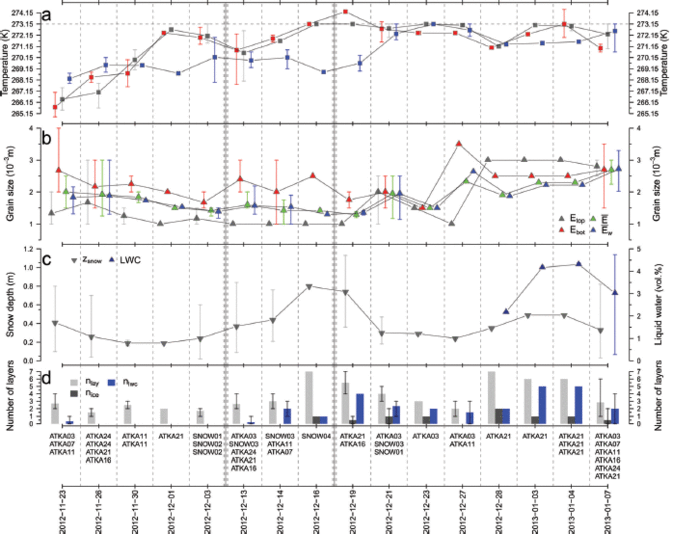
For clarification, Ebot gives the grain size of the lowest layer in the snowpack that is still snow, i.e. Ebot potentially states values several cm above the snow/ice interface. This was necessary due to the frequent presence of ice layers in the bottommost part of the snowpack, which do not yield any grain-size information. This happened especially during the later stages of the field campaign. The density measurements (not shown) were used to calculate the bulk snow-water equivalent (SWE, not shown) for each snow pit, but were otherwise omitted from all calculations, due to the limited number of measurements per pit and their low vertical resolution. The course of SWE is naturally very similar to that of zsnow and is therefore not shown.

Due to logistical constraints, we were not able to collect snow samples to estimate snowpack salinity for all snow-pit measurements. Salinity is, however, a crucial parameter in determining a⁰, due to its influence on the dielectric properties of snow and sea ice and its impact on the penetration depth. This shortcoming represents an obstacle for the interpretation of temporal backscatter changes. Reference DierkingDierking (2013) states a typical penetration depth of 0.03-0.15 m for X-band SAR on first-year sea ice under dry snow conditions. Reference BarberBarber and others (1995) showed that the snow/ ice interface temperature influences the brine volume fraction. This rise in brine volume fraction leads to an increase in the dielectric constant in the sea-ice surface, which again increases a⁰. However, the snow basal layer is also likely to have high salinity values (Reference MassomMassom and others, 2001), which might mask out underlying changes in the sea ice, especially after the onset of freeze/thaw cycles and in the presence of liquid water (Yackel and others, 2007).

Similar to the records of 2 m air temperature (Fig. 2a), the averaged snowpack temperature values (Fig. 3a) of all snow-pit measurements acquired on a given day increased towards the freezing point, and Ta as well as T_s reached this as early as 16 December 2012. Because of this, we considered all measurements after 16 December 2012 as being after the onset of early freeze/thaw processes.

Satellite measurements

TerraSAR-X is a spaceborne side-looking X-band SAR instrument run by the German Aerospace Center (DLR). The satellite has been operational since June 2007 in a polar orbit at 514 km altitude and can operate in four different imaging modes. Relevant to this study are the ScanSAR mode (SC) in single polarization and StripMap mode (SM) in single and dual polarization, due to their capability to sufficiently cover Atka Bay. The swath width changes with mode and polarization. In ScanSAR mode, a swath covers a ground area of 150 x 1 0 0 km². In StripMap mode, the coverage changes to 50 x 30 km² (50 x 15 km²) in single (dual) polarization mode (Reference Fritz and EinederFritz and Eineder, 2008).

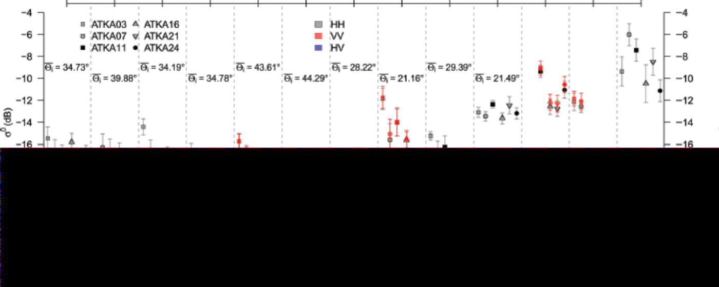
A total of 13 TerraSAR-X swaths were obtained before and during the field campaign (Table 1). Five scenes were recorded in single HH-polarization SC mode, while four scenes were acquired in dual-polarization SM mode in HH/ VV configuration and two in HH/HV. Additionally, two scenes were acquired in single HH-polarization SM mode. All TSX scenes were radiometrically calibrated using a commercial software package (SARscape) and georeferenced on a common pixel size of 25m. Due to increasing pixel size by multi-looking, the effect of speckle was reduced. The equivalent number of looks (ENL) increased by the grade of multi-looking, which depends on the initial pixel size (e.g. SC: 18.5 m; SM dual: 6.6m; and SM single: 3.3 m (Table 1)). It is important to note that the noise-equivalent sigma zero (NESZ) level is 19 dB. All pixel values below the NESZ are influenced by system noise and were excluded from further investigation as a precaution (Fig. 4).

Fig. 4. Temporal evolution of the TSX backscatter (<^r0) for all available TSX swaths and polarizations (HH = black, VV = red, HV = blue). Shown is the average ðˆ ⁰ for a 5 pixel x 5 pixel raster of each main study site (different symbols). Error bars indicate two standard deviations. Due to the smaller spatial coverage of the TSX StripMap mode, not all ATKA03-ATKA24 sites are covered by each swath. Additionally, the mean local incidence angle, 9 _i, is shown and the number of matched snow-pit measurements is given in parentheses (including match-ups with system-noise-influenced ˆ ⁰ values). Values influenced by the system noise, i.e. the noise-equivalent sigma zero (NESZ), are highlighted by the grey area at the bottom. Date format is yyyy-mm-dd.

Table 1. Overview of TSX data, including initial acquisition resolution, swath coverage and minimum/maximum local incidence angles (LIA). SC/SM indicate the TerraSAR-X acquisition mode of ScanSAR/StripMap. HH/VV/HV indicate the polarization as a combination of transmitted and received signal. Start and end time give the time of acquisition in UTC of each TSX swath. Also shown are the number of snow-pit measurements assigned to each TSX swath

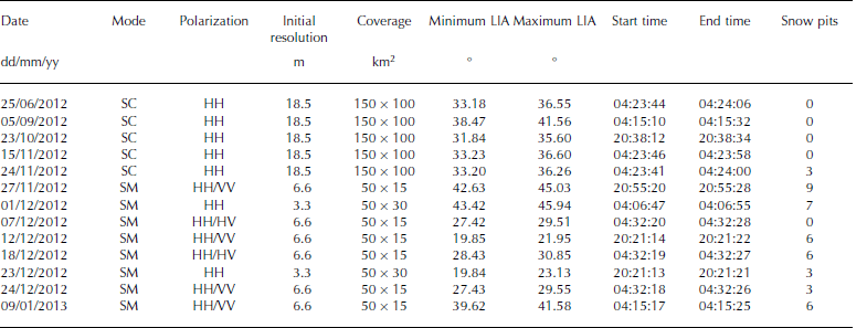
Due to logistical constraints, the number of snow-pit measurements directly matching a coincident TSX swath is very low (Fig. 2). Unfortunately, the two temporal matches between snow-pit measurements and TSX acquisitions could not be incorporated into our analysis. The respective TSX σ⁰ value of the first coincident match was influenced by system noise, while the second snow pit fell outside the TSX StripMap image. We chose to extract the average TSX backscatter values, σ⁰, of a 5 pixel x 5 pixel raster (i.e. 125 x 1 2 5 m²), along with its standard deviation at the position of each snow-pit measurement. To link as many snow-pit measurements as possible to the TSX backscatter extracts, we used the TSX data from all available swaths in a ±5 day range of each snow-pit measurement. By doing so, we were able to match at least one TSX σ⁰ record with one of our snow-pit measurements, despite differences in spatial coverage of each TSX swath.

While this approach is not ideal given the synoptic-scale atmospheric changes that can influence the snowpack during a 5 day window, we tried to reduce the influence of known meteorological events. Following the lack of observational snow data during the storm, we excluded the TSX swath of 7 December 2012 from our analysis. Also we did not match snow-pit measurements recorded before the second snowfall event on 17 December 2012 with TSX swaths acquired after that snowfall event (Fig. 2 and 3). This left us with 35 match-ups, excluding those with system-noise-influenced σ⁰ values. The majority of these data pairs (22) show a maximum temporal difference of 2 days. Five cases each have a time lag of 3 or 4 days, and three cases a time lag of 5 days.In the following, we explore information regarding resolution, coverage, acquisition time and local incidence angle of the TSX data (Table 1). In order to account for the wide range of local incidence angles (LIAs) covered by the TSX swaths (Table 1), we divided our dataset into three different LIA classes (LIA1: LIA> 36°; LIA2: 36° > LIA>27°; and LIA3: LIA < 27°), so as to review similar TSX swaths together. We chose this approach in order to examine the potential influences on the TSX er⁰ signal of different snowpack parameters on different LIAs. Due to the bipolar temporal distribution of the TSX swaths by means of acquisition time (early morning/late evening), no further steps were taken to account for diurnal variations in the signal.

Correlation coefficients were calculated to analyse relationships between individual snowpack parameters and corresponding TSX er⁰ values. In addition, simple linear regression models were fitted to the σ⁰ values and snowpack parameter groups to investigate the power and significance of the correlation, as well as the significance of the explained σ⁰ variance. Finally, we fitted a simple multiple linear regression model to our different datasets, to investigate its potential for maximizing the explained σ⁰ variance with a minimum of snowpack parameters per LIA class. Due to the limited number of matched snow-pit and TSX-swath measurements, the focus lies on the extracted HH-like polarization TSX backscatter data, hereafter named σ⁰ _HH.

Spatio-temporal snowpack changes

Because of the irregular temporal coverage of measurements at the different study sites and the different initial snowpack situation at each study site, further investigation of the various datasets (Fig. 3) is required. The observations taken on 23 and 26 November 2012 represent the late-winter setting of a still relatively cold environment (Fig. 2a and 3a). At this stage, at all main study sites (ATKA03-ATKA24) measurements were taken once, with ATKA07/16 at the upper end of the spectrum with regard to snow depth, number of layers and bottom-layer grain sizes and ATKA11/ 24 at the lower end.

Proceeding in time, a general increase in surface temperature, T_s, and air temperature, T _a, was noticeable. However, the snow/ice interface temperature, T _i, remained fairly constant, only varying with snow depth (Fig. 3a and c). On 16 December 2012, temperature measurements of T _a above the freezing point and T_s at the freezing point were recorded, followed by an increase in Ti. This led to near-isothermal snow conditions.

Between the initial conditions on 23/26 November 2012 and the end conditions on 7 January 2013, when coincident sampling at all main study sites took place again, an average increase and vertical equalization of the grain-size parameters occurred (Fig. 3b). This was driven by the equitemperature metamorphism processes in the snowpack (Reference FierzFierz and others, 2009). Furthermore, our few direct measurements of liquid-water content covered the whole spectrum between 1 and 5 vol.% on 7 January 2013. Such a range is expected to significantly affect the received backscatter signal (e.g. Yackel and Barber, 2007). In general, liquid water was found throughout the snow column (Fig. 3d), with the exceptions of 23 November 2012 and 13 December 2012, when flooded slush layers occurred at the snowpack base (ATKA11 and ATKA16).

Following the onset of freeze/thaw cycles and early melt, the degree of snowpack stratification increased, with an increase in the number of layers in general and in ice layers (Fig. 3d). Note that average values are shown, which might lead to the false impression that the degree of stratification falls off again at the end of the field campaign.

Spatio-temporal backscatter variations

Analysing the spatio-temporal variations of the TSX backscatter (σ⁰; Fig. 4), one needs to consider that not all study sites were covered in each swath (Table 1). We consider the HH-polarization data (Fig. 4, black) in SC and SM modes as well as the VV-polarization data (red) and the HV cross-polarization data (blue) in SM mode. Observed differences between the measurements at both HH and VV polarization are fairly small, while cross-polarization yields generally lower backscatter values. However, variations between the study sites can be large.

In the extracted TSX backscatter values of the first four swaths, there was an increasing spread in σ⁰ between the different study sites, in addition to a steady overall decrease in a₀. In particular, ATKA21 peaks compared with the other study sites, despite differences in σ⁰ due to different average LIA, 6 i . It should be added that the very low values of σ⁰ for the first few swaths are very close to or below the noise floor of TSX, which starts influencing the received signal below a threshold of 1 9 dB (worst case)/-22dB (normal) as stated by Reference Fritz and EinederFritz and Eineder (2008). However, the TSX data used in the later analyses were generally well above this noise floor and are unlikely to have been affected by it.

The X-band SAR microwave radiation did not significantly interact with the present dry snowpack in the early TSX swaths; this is consistent with the observations of Reference DierkingDierking (2013) and Reference Drinkwater, Hosseinmostafa and GogineniDrinkwater and others (1995). The spatial differences (Fig. 4) for the first four swaths are primarily linked to localized growth conditions during sea-ice formation and differing sea-ice compositions (salinity, proportion of incorporated frazil ice, columnar ice and platelet ice) which each affect the X-band SAR microwave radiation in a different way (e.g. Reference DierkingDierking, 2013). The small decrease in σ⁰ overtime (on average ∼2 dB) is probably due to a decrease in brine volume fraction in the snow-basal layer, as well as the ice-surface layer, due to low winter temperatures and still increasing ice thickness, which decreases the dielectric constant. This was noted for C-band SAR time series (e.g. Yackel and Barber, 2007) and also seems applicable for X-band SAR data. However, our data are not sufficient to assess this quantitatively. The comparably high σ⁰ values on 24 November 2012, despite the large local incidence angle, might be correlated to the increase in temperature around 20/21 November 2012 and the subsequent drop in temperature by ∼10 K (Fig. 2a). Unfortunately, there are no in situ temperature observations to verify this.

Reference HoppmannHoppmann and others (2015) discuss the different types of sea ice at Atka Bay and their structures. Their description of the primary ice-formation processes can be linked to the σ⁰ signals (Fig. 1 and 4) before the onset of melt and freeze/ thaw cycles. In areas where dynamical-growth processes dominated, σ⁰ is generally higher (e.g. the area around ATKA03/07). This results from the presence of pressure ridges that increase the surface scattering of the X-band radiation (Reference ErikssonEriksson and others, 2010). The highest signal is returned from the area of second-year sea ice close to the western ice-shelf edge. Here volume scattering is increased by air bubble inclusions, as well as surface scattering by the overall deformed structure of the ice. This adds up to a higher overall signal. An area of thermodynamic growth (ATKA21/24) generally has level ice with lower backscatter values (e.g. Reference DierkingDierking, 2013).

Across all incidence angles, there is an increase in σ⁰ over the field study. For LIA of 34-35°, there is an average increase of 10-12 dB in σ⁰ for all ATKA stations between 15 November 2012 and 9 January 2013. A similar, but smaller, increase was found for swaths with an average LIA of ∼29°. However, considerable spatial variability was evident, with ATKA11 exhibiting the highest variability.

The high σ⁰ values in the 9 January 2013 swath very likely originate from several freeze/thaw cycles, especially between 31 December 2012 and 5 January 2013 (Fig. 2a). These potentially increased the amount of volume scattering, through the formation of ice layers and an increase in grain sizes (Reference Willmes, Haas and NicolausWillmes and others, 2011). A steady increase in snow surface and snow/ice interface temperature and grain enlargement is seen in our measurements (Fig. 3a and b). Also, more stratification and an increased number of ice layers occur after the onset of freeze/thaw processes. All this potentially raises the returned backscatter. Nothing can be said about LIA3, due to the limited number of swaths and measurements taken in this LIA class.

The general increase in σ⁰ can be attributed to significant volume scattering by the snow basal-layer grains at ∼ 1 -3 vol.% of liquid water. With increasing liquid-water content, surface scattering further contributes to the overall signal (Reference BarberBarber and others, 1994; Reference BarberBarber, 2005).

Relationship between backscatter and snowpack characteristics

Here we correlate σ⁰ _HH and the previously discussed snow-pack parameters (Table 2; only significant correlations are shown). The statistical parameters include the correlation coefficient, R, the stability index, R², stating the explained variance, the p-value of the calculated f-test, p, stating the level of significance of the regression, and the sample size, n, as well as the statistical power. Power gives the probability that the H0 hypothesis is rejected (i.e. there is no correlation), where H0 is truly false (Reference CohenCohen, 1988).

Table 2. Summary of statistical parameters explaining the relationship between TSX backscatter σ ⁰ _HH and snowpack parameters (only parameters with significant correlations are shown, a = 0.95). Presented are the correlation coefficient, R, the stability index, R², the p-value of the calculated f-test, p, the sample size, n, and the statistical power. The results are shown per LIA class and data subset, where ALL equals all measurements per LIA class, SDS indicates a snow data subset of sites with z _snow < 0.6 m and EMO corresponds to measurements after the onset of early melt

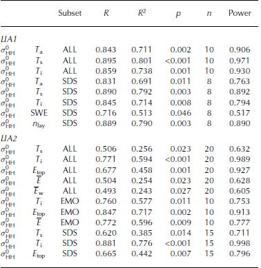
The results of Table 2 indicate a rather moderate dependency of observed σ⁰ _HH on the chosen snowpack parameters. However, there is a recurring set of snowpack parameters showing significant correlations to different degrees for all LIA classes and most data subsets. However, the rather low-to-moderate correlation coefficients and stability indices, as well as the low power values, have to be considered and are constrained by the small sample size. For LIA3, there were not enough samples to conduct meaningful calculations.

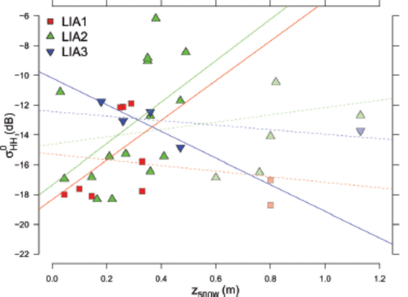
After visual screening and simple linear model iterations to find the best fit, we found that subsetting the dataset to measurements taken on snowpacks with a maximum depth of 0.60 m reveals a significantly higher correlation between zsnow and σ⁰ _HH for all LIA classes (Fig. 5). While 0.60m of snow is rather thick for Antarctic sea ice, 8 out of 35 of our snow-pit measurements featured a snow depth exceeding this threshold, while still being representative for their general area. However, these correlations are not necessarily significant (Table 1), given a level of significance (a) of 0.95, but exclusion of our very deep snow-pit measurements is likely to influence the correlations of other snowpack parameters to σ⁰ _HH (e.g. the snow/ice-surface temperature due to the X-band signal penetration depth (Table 2)).

Fig. 5. Scatter plot of snow depth (z _snow) against TSX HH backscatter (σ0H_H). Shown are the snow depths and their corresponding local incidence angle (LIA) class-based σ ⁰ _HH values. Value pairs above/below the 0.6 m threshold are plotted transparent/solid. The corresponding regression lines are shown, where solid lines correspond to the value pairs with z _snow<0.6m and dashed lines are for the complete dataset.

Neglecting the scatter loss, we calculated the theoretical penetration depths from the bulk dielectric constant for a range of bulk snow liquid-water content and bulk snow densities from our measurements, by solely considering the absorption loss. This was done using the governing equations for wet snow provided by Reference Hallikainen and WinebrennerHallikainen and Wine brenner (1992) A liquid-water content of 0.35-0.5 vol.%, for example, led to a penetration depth at TSX X-band of 0.4-0.75 m. This might explain the increase in correlation between σ⁰ _HH and, especially, Ti. At a snow liquid-water content of 1-3 vol.%, the theoretical penetration depth decreases to 0.05-0.20 m. However, given the temperature records (Fig. 2a), the high values of liquid water within the snow are likely to be snapshots of a constantly changing snowpack, due to thaw/refreeze cycling.

The overall most reliable results were found for the LIA2 class (Table 2), i.e. LIA 36-27°, where sufficient sample size corresponds to the high statistical power of the significant correlations. Snow/ice interface temperature, T _i, and top-layer grain size, E _top, showed significant correlation coefficients (p < 0.01) with high power values close to 1. This implies (with high confidence) that the results are not based on random noise. These numbers change slightly, depending on the subset used. Limiting ourselves to measurements with snow depths of <0.6 m (SDS), the correlation coefficient and stability index for the snow/ice interface temperature, T _i, increase, probably due to their capturing the penetration depth of X-band radar. For greater snow depths, the ice/snow interface becomes invisible, due to the limited penetration depth of X-band radar (Yackel and Barber, 2007).

We chose an approach to evaluate the amount of variance in our TSX σ⁰ _HH that can be explained by the snowpack parameters, by using a simple multiple linear model. Each model estimate started with all the snowpack parameters as input. Using stepwise regression modelling, the parameter with the highest p-value (i.e. the least significant contribution to the overall explained variance, R² , was removed from the model at each iteration. After several iterations, a significant model fit was achieved in most cases. The iteration stopped when, in a subsequent step, the overall explained variance dropped significantly and the model significance decreased. However, no significant model fits could be found for some LIA classes and data subsets, due to the limited sample size (especially for the LIA3 class).

The model name tags (Table 3) correspond to the underlying data subsets (e.g. limited to measurement sites with z _snow < 0.6 m (SDS) or after the onset of early-melt processes on 16 December 2012 (EMO)). Table 3 also shows the sample size, n, the p-value of the calculated f-test, p, and the stability index, R ² _a dj. The latter is corrected (adjusted) for the different amount of predictors which can lead to an increased general stability index, R2. All model fits are significant and explain 76-93% (R ² _adj) of their representative observed σ⁰ _HH variance.

Table 3. Different model fits to the TSX backscatter σ ⁰ _H H data. Presented are the sample size, n, the p-value of the calculated f-test, p, the adjusted stability index, R ² _ad that shows the explained variance adjusted for the different amount of predictors, and the predictors of σ ⁰. Also shown is the root-mean-squared error of the cross validation (dB; RMSE). Model fits are identified by tags based on the LIA and data limitations, where SDS stands for snow-depth subset and EMO means early-melt onset

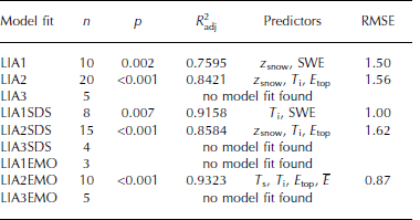
To evaluate the quality of our model fits we chose a cross-validation approach, due to the limited sample size. Here the model was set up with the significant predictors calculated from the complete sample size, n, but based on a sample size of n 1. Iteratively, each member of the initial sample was excluded from the set-up, and was instead calculated by the model. The root-mean-squared error (RMSE) between the modelled and observed σ⁰ _HH values was then calculated. The results (Table 3) vary between 0.87 and 1.62 dB (LIA2EMO and LIA2SDS, respectively). These compare favourably with the absolute/relative radiometric accuracy of the TSX sensor (0.6/0.3 dB; Reference Fritz and EinederFritz and Eineder, 2008). However, the quite high stability indices of >90% were achieved on very small datasets with a comparably large number of predictors.

During the cross validation, it became clear that the σ⁰ _HH signatures of certain snow-pit measurements are more difficult to derive from the various model fits using different predictor set-ups, i.e. excluding those snow-pit measurements drastically decreased the RMSE, compared with the RMSE changes of the remaining iterations. An example is ATKA11. We attribute this to the recurrent surface flooding and refreezing that occurred during the course of our field campaign, which cannot be explained sufficiently with the snowpack parameters used here.

Fig. 6. Four different multiple linear model fits (a-d) (red triangles) to the extracted σ ⁰ _H H values from all available snow-pit measurements in a ±5 day range (grey dots). (a) Based on all available snow-pit measurements for LIA1. (b) Limited to snow-pit measurements with zsnow < 0.6 m for LIA1. (c, d) the same set-ups as (a, b) for LIA2. All model fits are significant (a < 0.001) and explain 76-91% (R _{a d}j_j) of the total variance of σ0HH. Date format is yyyy-mm-dd.

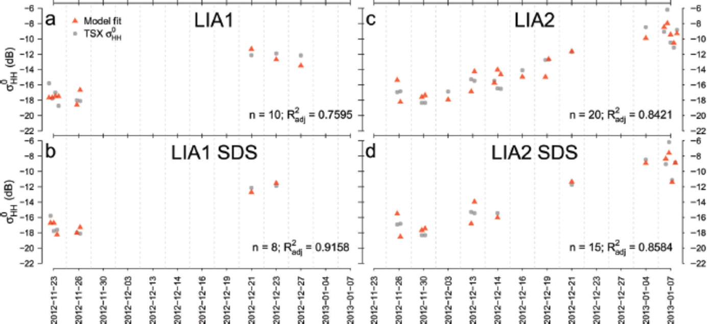
The significant snow parameters (Table 2) also appear as model predictors in Table 3. Furthermore, the snow depth and snow water equivalent are significant contributors to the overall variance, despite showing non-significant correlations with σ0HH by themselves. While there are definitive internal correlations (e.g. between zsnow and SWE, or the temperature parameters), they are not interchangeable without a large drop in the stability indices. Four representative model fits are discussed here (Fig. 6; grey dots indicate the measured TSX σ0HH values; red triangles correspond to the modelled backscatter). Model fit LIA1 (Fig. 6a) explains 76% (R 2adj) of the σ0HH variance, spans a sample size often value pairs and is based on the predictors zsnow and SWE (Table 3). Model fit LIA2 (Fig. 6c) explains 84% (R 2adj) of the σ0HH variance, spans a larger sample size of 20 value pairs and is based on the predictors zsnow, Ti and Etop. Furthermore, the overall temporal coverage of pre-meltonset conditions as well as post-melt-onset conditions is better represented in the LIA2 than the LIA1 data. In combination with the larger sample size, this gives higher confidence in the general quality of the model fit to the LIA2 data. However, the dataset is too limited to further investigate differences between the different LIA classes.

The corresponding equations for the four model fits are:

(1)

(2)

(3)

(4)

where σ0 represents the modelled backscatter values, z _snow is the snow depth (m), SWE is the snow water equivalent (kgm^-2 ), T _i is the snow/ice interface temperature (K) and E _top is top-layer grain size (m).

All model fits are more sensitive to changes in grain size or temperature parameters (large slopes) than to snow depth or snow water equivalent (small slopes), based on Eqns (1-4). Even small changes in grain size and temperature predictors have a higher impact on the modelled backscatter. However, the snow depth shows a much higher spread in our dataset (Fig. 5) compared with the small spectrum of different top-layer grain sizes (Fig. 3b).

As stated by, for example, Yackel and Barber (2007) and Reference BarberBarber (2005), the snow/ice interface temperature as it affects the dielectric properties of the basal-snow layer (liquid-water content and brine volume fraction) is crucial for explaining the received radar backscatter. Although we did not measure snow salinity, the importance of snow/ice interface temperature is apparent in our results. Related as they are to the liquid-water content, snow grain size and volume are important determinants of volume scattering in the snowpack. Both are also reflected in our results, especially for the LIA2 class.

Because of the limited sample size, the additional potential of VV like-polarization and HV cross-polarization acquisitions could not be taken into account. It is expected that this capability will improve the retrieval of the physical properties of snow on Antarctic sea ice from X-band SAR backscatter data, but additional measurements and further investigation are necessary. This potential is underlined by the spatial and temporal differences between the like/like and like/cross-polarization TSX StripMap images (Fig. 4) for the different study sites. We were able to show that both the snow cover and the snow/ice interface have a strong influence on the TSX σ⁰ _HH signal. However, there are sources of error and uncertainties, due in large part to the lack of simultaneous daily measurements of snow physical properties and TSX swath coverage. Nonetheless, the onset of melt processes and freeze/thaw cycles is clearly recognizable in the X-band SAR backscatter time series.