





1. Introduction
We study a new preferential attachment model with edge detachment, closely linked to birth–death models in evolutionary dynamics [Reference Manrubia and Zanette22, Reference Maruvka, Kessler and Shnerb23] and somewhat different from established models [Reference Deijfen and Lindholm13, Reference Dorogovtsev and Mendes17, Reference Vallier31, Reference Wu, Dong, Liu and Cai32]. We use an embedding into a generalized Yule model [Reference Lansky, Polito and Sacerdote21] to show that there are different asymptotic regimes for the tail of the in-degree distribution. Our main point is that through this embedding, the description of these different regimes is particularly neat, and our results may be seen as another illustration for the efficiency of embedding techniques [Reference Athreya1, Reference Athreya, Ghost and Sethuraman2, Reference Bhamidi6, Reference Rudas, Tóth and Valkó28].
Preferential attachment models are well-studied discrete-time random graph models in which new vertices are successively added and connected to an existing vertex with a probability proportional to an increasing function of its in-degree. This mechanism is well suited to model a diverse range of phenomena, such as the concentration of resources in a market environment or the concentration of links in a communication network. The vertices represent market participants or network nodes, while the incoming edges represent the allocation of resources or directed communication channels. Motivated by such applications, we include a mechanism of edge detachment: it is not atypical that the allocation of goods from one party to another stops due to changed market conditions or that communication links disappear spontaneously by a sudden loss of attention.
In [Reference Yule33] Yule studied a continuous-time model for the creation of families and the evolution of individuals within them. In [Reference Simon29] Simon studied a discrete-time model to describe the appearance of new words in a large piece of a text. For suitable parameters both models lead to the same asymptotic distribution, called the Yule–Simon distribution. In the recent article [Reference Lansky, Polito and Sacerdote21] a generalized Yule model was proposed, where the original pure birth process governing the growth of individuals within a family was replaced by a birth–death process with fertility and mortality rates $\lambda$
and
$\lambda$
and $\mu$
, respectively. The authors obtained the limit distribution of the size of a randomly chosen family and observed different behaviour in the supercritical regime
$\mu$
, respectively. The authors obtained the limit distribution of the size of a randomly chosen family and observed different behaviour in the supercritical regime $\lambda>\mu$
, the subcritical regime
$\lambda>\mu$
, the subcritical regime $\lambda<\mu$
, and the critical regime
$\lambda<\mu$
, and the critical regime $\lambda=\mu$
. Their simulations show a heavy-tail power law in the supercritical regime, a much more rapid decay in the subcritical, and an intermediate decay in the critical.
$\lambda=\mu$
. Their simulations show a heavy-tail power law in the supercritical regime, a much more rapid decay in the subcritical, and an intermediate decay in the critical.
The first references for preferential attachment models in the context of random graphs were [Reference Barabási and Albert4, Reference de Solla Price16]. The limit degree distribution of these models as the number of vertices goes to infinity was studied rigorously in [Reference Bollobás, Riordan, Spencer and Tusnády7]; it coincides with the Yule–Simon distribution for specific parameters. Numerous generalizations of [Reference Barabási and Albert4] were investigated; see, for example, [Reference Berger, Borgs, Chayes, Dśouza and Kleinberg5, Reference Cooper and Frieze9, Reference Cooper and Pralat11, Reference Deijfen, van den Esker, van der Hofstad and Hooghiemstra14, Reference Dereich and Ortgiese15, Reference Dorogovtsev, Mendes and Samukhin18–Reference Krapivsky, Redner and Leyvraz20, Reference Oliveira and Spencer25, Reference Pachon, Sacerdote and Yang27]. Links to continuous-time Markov processes were studied in [Reference Athreya1, Reference Athreya, Ghost and Sethuraman2, Reference Bhamidi6, Reference Rudas, Tóth and Valkó28]. Models with edge detachment were considered in [Reference Chung and Lu8, Reference Cooper, Frieze and Vera10, Reference Deijfen and Lindholm13, Reference Dorogovtsev and Mendes17, Reference Wu, Dong, Liu and Cai32]. In [Reference Chung and Lu8, Reference Cooper, Frieze and Vera10] it was shown that the degree distribution follows a power law whose exponent depends on the attachment and detachment probabilities. In [Reference Dorogovtsev and Mendes17] it was shown that detachment changes the graph more drastically than mere attachment. In [Reference Deijfen and Lindholm13, Reference Wu, Dong, Liu and Cai32] the authors observed a phase transition in the expected empirical degree distribution with a power-law decay in the supercritical regime and an exponential decay in the subcritical. The model in [Reference Wu, Dong, Liu and Cai32] is very similar to special cases in [Reference Chung and Lu8, Reference Cooper, Frieze and Vera10]. Both [Reference Deijfen and Lindholm13, Reference Wu, Dong, Liu and Cai32] gave a critical threshold, but only an incomplete description of the possible parameter regimes. A first complete description was given in [Reference Vallier31], including the observation that the decay at the threshold is strictly intermediate.
Here we introduce a different model, partially motivated by two specific birth–death models [Reference Manrubia and Zanette22, Reference Maruvka, Kessler and Shnerb23]. At each time step we either add a vertex and a loop attached to it, or create an edge following preferential attachment, or delete an edge following preferential detachment. A precise description is given in Section 2. In contrast to [Reference Vallier31], the parameters in our model are not probabilities but rates, and the attachment–detachment probabilities are obtained as the products of these rates with the percentage of oriented edges pointing to the respective vertex. We allow new vertices without connecting edges to existing vertices, but always attach a loop to them, so that they immediately compete in attracting new edges. In the attachment–detachment probabilities this leads to a renormalization by division through an affine function of in-degrees, which is different from the linear denominators in [Reference Deijfen and Lindholm13, Reference Vallier31, Reference Wu, Dong, Liu and Cai32] and in traditional preferential attachment models. By this construction the model embeds naturally into a generalized Yule model, and by this embedding it inherits the limit behaviour proved in [Reference Lansky, Polito and Sacerdote21].
Similarly to [Reference Vallier31], we prove a complete description of the different asymptotic regimes for the limit in-degree distribution of a vertex chosen uniformly at random: power-law decay in the supercritical, exponential decay in the subcritical, and a ‘strictly intermediate’ decay in the critical. In [Reference Vallier31] the exponents and the critical threshold are simple algebraic functions of the attachment–detachment probabilities. In our model, the exponents are even simpler functions, but of the rates. The different regimes and the critical threshold can immediately be read off the parameter constellation, so that no calculation is necessary; see Theorem 1. Moreover, they admit particularly transparent interpretations, cf. Remark 1. In the power-law regime of the model in [Reference Vallier31] any exponent in $[2,\infty)$
can be achieved through the choice of suitable probabilities. In our model the even wider range
$[2,\infty)$
can be achieved through the choice of suitable probabilities. In our model the even wider range $(1,\infty)$
is accessible through suitable parameter choices.
$(1,\infty)$
is accessible through suitable parameter choices.
Another related paper is [Reference Deijfen12], where a continuous-time network model was studied. There the vertex population evolves as a supercritical birth–death process. New links to existing vertices and the death of such vertices are governed by a fitness parameter. The fitness of a vertex is its cumulative in-degree up to the present time; it takes into account current links and ‘ghost links’ to meanwhile deceased vertices. The author proved a similar phase transition between power-law, exponential, and intermediate regimes. For a corresponding model without ghost links they provided numerical simulations, but no rigorous calculations. Our model is based on the present in-degree – ghost links are excluded.
In Section 2 we provide a description of the model, and in Section 3 we state and discuss our main result on the limit in-degree distribution, Theorem 1. The generalized Yule model is explained in Section 4 – a detailed construction is given in Appendix A. In Section 5 we provide the embedding result, Theorem 2, which might be of independent interest, and a more detailed variant of Theorem 1; see Theorem 3. To make the article largely self-contained, we recall some known facts in Appendices B and C.
We use the notation $\mathbb{N}=\{1,2,\ldots\}$
and
$\mathbb{N}=\{1,2,\ldots\}$
and $\mathbb{N}_0\,:\!=\,\mathbb{N}\cup\{0\}$
. Given functions
$\mathbb{N}_0\,:\!=\,\mathbb{N}\cup\{0\}$
. Given functions $f,g\colon(0,+\infty)\to\mathbb{R}$
or
$f,g\colon(0,+\infty)\to\mathbb{R}$
or $f,g\colon\mathbb{N}\to\mathbb{R}$
, we write
$f,g\colon\mathbb{N}\to\mathbb{R}$
, we write $f\sim g$
if
$f\sim g$
if $\lim_{j\rightarrow\infty} {f(j)}/{g(j)} = 1$
. We use
$\lim_{j\rightarrow\infty} {f(j)}/{g(j)} = 1$
. We use $\textbf{B}$
to denote the Beta function,
$\textbf{B}$
to denote the Beta function,
 \begin{align*}\textbf{B}(a,b)=\int_0^1s^{a-1}(1-s)^{b-1}\,{\mathrm{d}} s,\quad a > 0,\ b > 0,\end{align*}
and $\mathbf{U}$
to denote the confluent hypergeometric function,
$\mathbf{U}$
to denote the confluent hypergeometric function,
 \begin{align*}\mathbf{U}(a,b,z)=\frac{1}{\Gamma(a)}\int_0^\infty{\mathrm{e}}^{-zs}s^{a-1}(1+s)^{b-a-1}\,{\mathrm{d}} s,\quad a > 0,\ b > 0,\ z > 0;\end{align*}
here $\Gamma$
is the Euler gamma function. We denote the Gauss hypergeometric function by
$\Gamma$
is the Euler gamma function. We denote the Gauss hypergeometric function by ${}_2\mathbf{F}_1$
:
${}_2\mathbf{F}_1$
:
 \begin{align*}{}_2\mathbf{F}_1(a,b,c,z)=\frac{1}{\mathbf{B}(b,c-b)}\int_0^1s^{b-1}\frac{(1-s)^{c-b-1}}{(1-sz)^a}\,{\mathrm{d}} s,\quad a > 0,\ b > 0,\ c > 0,\ 0 < z < 1.\end{align*}
2. A random graph model with edge detachment
The model we study can be described as a random graph process $(G_t^{\lambda_1,\lambda_2,\mu_2})_{t\in\mathbb{N}_0}$
with discrete time
$(G_t^{\lambda_1,\lambda_2,\mu_2})_{t\in\mathbb{N}_0}$
with discrete time $t\in \mathbb{N}_0$
and with parameters
$t\in \mathbb{N}_0$
and with parameters $ \lambda_1,\lambda_2>0$
and
$ \lambda_1,\lambda_2>0$
and $\mu_2\geq 0$
. At each time t, a realization of the process is a directed graph
$\mu_2\geq 0$
. At each time t, a realization of the process is a directed graph $G_t^{\lambda_1,\lambda_2,\mu_2}(\omega)$
with vertex set
$G_t^{\lambda_1,\lambda_2,\mu_2}(\omega)$
with vertex set $V_t(\omega)\subset \mathbb{N}$
. The process starts at time
$V_t(\omega)\subset \mathbb{N}$
. The process starts at time $t=0$
as a graph
$t=0$
as a graph $G_0^{\lambda_1,\lambda_2,\mu_2}$
consisting of the single vertex 1 and a directed loop attached to it. The number of vertices at time t is given by the random variable
$G_0^{\lambda_1,\lambda_2,\mu_2}$
consisting of the single vertex 1 and a directed loop attached to it. The number of vertices at time t is given by the random variable $|V_t|$
; here
$|V_t|$
; here $|M|$
denotes the cardinality of a finite set M. For any t and any
$|M|$
denotes the cardinality of a finite set M. For any t and any $i\in \mathbb{N}$
we set
$i\in \mathbb{N}$
we set $d_t^i=0$
on the event
$d_t^i=0$
on the event $\{|V_t|<i\}$
, while on the event
$\{|V_t|<i\}$
, while on the event $\{|V_t|\geq i\}$
we define
$\{|V_t|\geq i\}$
we define $d_t^i$
to be the in-degree of the vertex i at time t. The transition from
$d_t^i$
to be the in-degree of the vertex i at time t. The transition from $G_t^{\lambda_1,\lambda_2,\mu_2}$
to
$G_t^{\lambda_1,\lambda_2,\mu_2}$
to $G_{t+1}^{\lambda_1,\lambda_2,\mu_2}$
is governed by the given parameters: the parameter
$G_{t+1}^{\lambda_1,\lambda_2,\mu_2}$
is governed by the given parameters: the parameter $\lambda_1$
is a rate for the appearance of new vertices,
$\lambda_1$
is a rate for the appearance of new vertices, $\lambda_2$
is a rate for the appearance of new edges, and
$\lambda_2$
is a rate for the appearance of new edges, and $\mu_2$
a rate for the removal of edges. At time
$\mu_2$
a rate for the removal of edges. At time $t+1$
exactly one of the following three events happens:
$t+1$
exactly one of the following three events happens:
-
(i) A new vertex and a directed loop attached to it are added to $G_t^{\lambda_1,\lambda_2,\mu_2}$
. This event occurs with probability
$|V_t|\lambda_1\big(\sum_{j=1}^{|V_t|}(\lambda_1+\lambda_2d_t^{\,j}+\mu_2d_t^{\,j})\big)^{-1}$
.
$G_t^{\lambda_1,\lambda_2,\mu_2}$
. This event occurs with probability
$|V_t|\lambda_1\big(\sum_{j=1}^{|V_t|}(\lambda_1+\lambda_2d_t^{\,j}+\mu_2d_t^{\,j})\big)^{-1}$
. -
(ii) A directed edge emanating from the last vertex
$|V_t|$
of
$G_t^{\lambda_1,\lambda_2,\mu_2}$
and arriving at one of the vertices
$1,\ldots,|V_t|$
of
$G_t^{\lambda_1,\lambda_2,\mu_2}$
is added; here, vertex
$1\leq i\leq |V_t|$
is chosen with probability
$\lambda_2 d_t^i \big(\sum_{j=1}^{|V_t|}(\lambda_1+\lambda_2 d_t^{\,j}+\mu_2 d_t^{\,j})\big)^{-1}$
. -
(iii) A directed edge is removed from
$G_t^{\lambda_1,\lambda_2,\mu_2}$
; here, the probability of choosing an incoming edge adjacent to vertex
$1\leq i\leq |V_t|$
is
$\mu_2 d_t^i\big(\sum_{j=1}^{|V_t|}(\lambda_1+\lambda_2 d_t^{\,j}+\mu_2 d_t^{\,j})\big)^{-1}$
.








To provide a formal description, we restrict attention to the vectors $(d_t^1,d_t^2,\ldots,d_t^{|V_t|})$
of vertex in-degrees of the random graphs
$(d_t^1,d_t^2,\ldots,d_t^{|V_t|})$
of vertex in-degrees of the random graphs $G_t^{\lambda_1,\lambda_2,\mu_2}$
,
$G_t^{\lambda_1,\lambda_2,\mu_2}$
, $t\in\mathbb{N}_0$
. Let
$t\in\mathbb{N}_0$
. Let
 \begin{equation} S\,:\!=\,\bigcup_{n\geq 1}\mathbb{N}_0^n.\end{equation}
Given $\mathbf{x}\in S$
, we write
$\mathbf{x}\in S$
, we write
 \begin{equation} \ell(\mathbf{x})\,:\!=\,n\quad \text{if}\ \mathbf{x}\in \mathbb{N}_0^n,\end{equation}
that is, if $\mathbf{x}=(x^1,x^2,\ldots,x^n)$
, and we call
$\mathbf{x}=(x^1,x^2,\ldots,x^n)$
, and we call $\ell(\mathbf{x})$
the length of
$\ell(\mathbf{x})$
the length of $\mathbf{x}$
. By
$\mathbf{x}$
. By $\delta_{(1)}$
we denote the point mass probability measure on S at the sequence (1) of length one and with the single element 1. We use the convenient shortcut notation
$\delta_{(1)}$
we denote the point mass probability measure on S at the sequence (1) of length one and with the single element 1. We use the convenient shortcut notation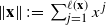 $\|\mathbf{x}\|\,:\!=\,\sum_{j=1}^{\ell(\mathbf{x})} x^{\,j}$
,
$\|\mathbf{x}\|\,:\!=\,\sum_{j=1}^{\ell(\mathbf{x})} x^{\,j}$
, $\mathbf{x}\in S$
. Given
$\mathbf{x}\in S$
. Given $\mathbf{x},\mathbf{y}\in S$
, let
$\mathbf{x},\mathbf{y}\in S$
, let
 \begin{align*} p_{\mathbf{x},\mathbf{y}} \,:\!=\, \begin{cases} \dfrac{x^i\lambda_2}{(\lambda_2+\mu_2)\|\mathbf{x}\|+\ell(\mathbf{x})\lambda_1}, & \mathbf{y}=(x^1,x^2,\ldots,x^{i-1},x^i+1,x^{i+1},\ldots,x^{\ell(\mathbf{x})}),\ 1\leq i\leq \ell(\mathbf{x}), \\[12pt] \dfrac{x^i\mu_2}{(\lambda_2+\mu_2)\|\mathbf{x}\|+\ell(\mathbf{x})\lambda_1}, & \mathbf{y}=(x^1,x^2,\ldots,x^{i-1},x^i-1,x^{i+1},\ldots,x^{\ell(\mathbf{x})}),\ 1\leq i\leq \ell(\mathbf{x}), \\[12pt] \dfrac{\ell(\mathbf{x})\lambda_1}{(\lambda_2+\mu_2)\|\mathbf{x}\|+\ell(\mathbf{x})\lambda_1}, & \mathbf{y}=(x^1,x^2,\ldots,x^{\ell(\mathbf{x})},1),\ 1\leq i\leq \ell(\mathbf{x}). \end{cases}\end{align*}
Now let
 \begin{equation} \mathbf{d}=(\mathbf{d}_t)_{t\in\mathbb{N}}\quad \text{with}\ \mathbf{d}_t=(d_t^1,d_t^2,\ldots,d_t^{\ell(\mathbf{d}_t)}), \ t\in\mathbb{N}_0,\end{equation}
be the uniquely determined discrete-time Markov chain with state space S, transition probabilities $(p_{\mathbf{x},\mathbf{y}})_{\mathbf{x},\mathbf{y}\in S}$
, and initial distribution
$(p_{\mathbf{x},\mathbf{y}})_{\mathbf{x},\mathbf{y}\in S}$
, and initial distribution $\delta_{(1)}$
. Ionescu-Tulcea’s theorem guarantees the existence of a probability space
$\delta_{(1)}$
. Ionescu-Tulcea’s theorem guarantees the existence of a probability space $(\Omega,\mathcal{F},\mathbb{P})$
such that
$(\Omega,\mathcal{F},\mathbb{P})$
such that $\mathbb{P}(\mathbf{d}_0=(1))=1$
and
$\mathbb{P}(\mathbf{d}_0=(1))=1$
and $\mathbb{P}(\mathbf{d}_{t+1}=\mathbf{y}\mid\mathbf{d}_t=\mathbf{x})=p_{\mathbf{x},\mathbf{y}}$
for all
$\mathbb{P}(\mathbf{d}_{t+1}=\mathbf{y}\mid\mathbf{d}_t=\mathbf{x})=p_{\mathbf{x},\mathbf{y}}$
for all $\mathbf{x},\mathbf{y}\in S$
and
$\mathbf{x},\mathbf{y}\in S$
and $t\in\mathbb{N}_0$
. We write
$t\in\mathbb{N}_0$
. We write ${\mathbb E}$
and
${\mathbb E}$
and $\mathbb{V}$
for the expectation and variance associated with
$\mathbb{V}$
for the expectation and variance associated with ${\mathbb P}$
, respectively.
${\mathbb P}$
, respectively.
3. Limit in-degree distributions and tail behaviour
For any $t\in \mathbb{N}_0$
, let
$t\in \mathbb{N}_0$
, let
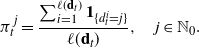 \begin{equation*} \pi_t^{\,j} = \frac{\sum_{i=1}^{\ell(\mathbf{d}_t)}\mathbf{1}_{\{d_t^i=j\}}}{\ell(\mathbf{d}_t)}, \quad j\in\mathbb{N}_0.\end{equation*}
Since $\ell(\mathbf{d}_t)$
equals the number
$\ell(\mathbf{d}_t)$
equals the number $|V_t|$
of vertices in
$|V_t|$
of vertices in $G_t^{\lambda_1,\lambda_2,\mu_2}$
, the random variable
$G_t^{\lambda_1,\lambda_2,\mu_2}$
, the random variable $\pi_t^{\,j}$
may be viewed as the number of vertices in
$\pi_t^{\,j}$
may be viewed as the number of vertices in $G_t^{\lambda_1,\lambda_2,\mu_2}$
having in-degree j. Let
$G_t^{\lambda_1,\lambda_2,\mu_2}$
having in-degree j. Let $d(V_t)$
be the random variable on
$d(V_t)$
be the random variable on $(\Omega,\mathcal{F},\mathbb{P})$
fully determined by the set of conditional distributions
$(\Omega,\mathcal{F},\mathbb{P})$
fully determined by the set of conditional distributions
 \begin{equation} {\mathbb P}(d(V_t)=j\mid\ell(\mathbf{d}_t)=n) = \frac{1}{n}\sum_{i=1}^n{\mathbb P}(d_t^i=j \mid \ell(\mathbf{d}_t)=n), \quad n\in\mathbb{N},\ j\in\mathbb{N}_0.\end{equation}
It may be viewed as the in-degree of a vertex chosen uniformly at random in $G_t^{\lambda_1,\lambda_2,\mu_2}$
. Conditioning on
$G_t^{\lambda_1,\lambda_2,\mu_2}$
. Conditioning on $\ell(\mathbf{d}_t)$
and using (4), we obtain
$\ell(\mathbf{d}_t)$
and using (4), we obtain
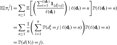 \begin{align*} {\mathbb E}[\pi_t^{\,j}] & = \sum_{n\geq 1}{\mathbb E}\Bigg[\Bigg( \frac{\sum_{i=1}^{\ell(\mathbf{d}_t)}\mathbf{1}_{\{d_t^i=j\}}}{\ell(\mathbf{d}_t)}\Bigg)\mid\ell(\mathbf{d}_t)=n\Bigg] {\mathbb P}(\ell(\mathbf{d}_t)=n) \\[3pt] & = \sum_{n\geq 1}\frac{1}{n}\Bigg(\sum_{i=1}^n{\mathbb P}(d_t^i=j\mid \ell(\mathbf{d}_t)=n)\Bigg) {\mathbb P}(\ell(\mathbf{d}_t)=n) \\[3pt] & = {\mathbb P}(d(V_t)=j).\end{align*}
That is, at any fixed time $t\in\mathbb{N}_0$
, the expectation under
$t\in\mathbb{N}_0$
, the expectation under $\mathbb{P}$
of the empirical in-degree distribution
$\mathbb{P}$
of the empirical in-degree distribution $(\pi_t^{\,j})_{j\geq 0}$
and the in-degree distribution
$(\pi_t^{\,j})_{j\geq 0}$
and the in-degree distribution ${\mathbb P}(d(V_t)=\cdot)$
under
${\mathbb P}(d(V_t)=\cdot)$
under $\mathbb{P}$
of a vertex chosen uniformly at random coincide.
$\mathbb{P}$
of a vertex chosen uniformly at random coincide.
Our main statement is about the limit of these in-degree distributions as $t\to\infty$
. It says that a limit distribution exists and follows different asymptotic regimes as
$t\to\infty$
. It says that a limit distribution exists and follows different asymptotic regimes as $j\to\infty$
.
$j\to\infty$
.
Theorem 1. Let $\lambda_1,\lambda_2>0$
and
$\lambda_1,\lambda_2>0$
and $\mu_2\geq 0$
, let
$\mu_2\geq 0$
, let $\mathbf{d}$
be as in (3), and let
$\mathbf{d}$
be as in (3), and let $d(V_t)$
be the random variable determined by (4). Then the limits
$d(V_t)$
be the random variable determined by (4). Then the limits
 \begin{equation} p_j\,:\!=\,\lim_{t\rightarrow\infty}{\mathbb P}(d(V_t)=j),\quad j\in\mathbb{N}_0, \end{equation}
exist. As $j\to\infty$
, the limit distribution
$j\to\infty$
, the limit distribution $(p_j)_{j\geq 0}$
shows the following asymptotic behaviour:
$(p_j)_{j\geq 0}$
shows the following asymptotic behaviour:
-
(i) If
$\mu_2=0$
, then
\begin{align*}p_j\sim c_1\,j^{-(1+{\lambda_1}/{\lambda_2})} \quad \text{with}\ c_1=\frac{\lambda_1}{\lambda_2}\Gamma\bigg(1+\frac{\lambda_1}{\lambda_2}\bigg).\end{align*}
-
(ii) If
$\mu_2>0$
and
$\lambda_2>\mu_2$
, then
\begin{align*}p_j \sim c_2 j^{-(1+{\lambda_1}/({\lambda_2-\mu_2}))} \quad \text{with}\ c_2=\frac{\lambda_1}{\lambda_2}\bigg(\frac{\lambda_2}{\lambda_2-\mu_2}\bigg)^{{\lambda_1}/({\lambda_2-\mu_2})} \Gamma\bigg(1+\frac{\lambda_1}{\lambda_2-\mu_2}\bigg).\end{align*}
-
(iii) If
$\mu_2>0$
and
$\lambda_2<\mu_2$
, then
\begin{align*}p_j \sim c_3\bigg(\frac{\lambda_2}{\mu_2}\bigg)^{j+1}\!\! j^{-(1+{\lambda_1}/({\mu_2-\lambda_2}))} \,\,\, \text{with}\ c_3=\frac{\lambda_1}{\mu_2}\bigg(\frac{\mu_2}{\mu_2-\lambda_2}\bigg)^{-{\lambda_1}/({\mu_2-\lambda_2})} \!\! \Gamma\bigg(1+\frac{\lambda_1}{\mu_2-\lambda_2}\bigg).\end{align*}
-
(iv) If
$\mu_2>0$
and
$\lambda_2=\mu_2$
, then
$j^mp(j)\to 0$
for any
$m\in \mathbb{N}$
but
${\mathrm{e}}^{\varepsilon j}p(j)\to +\infty$
for any
$\varepsilon>0$
.


For the expectation of a random variable $d(V_\infty)$
with distribution
$d(V_\infty)$
with distribution $(p_j)_{j\geq 0}$
we have
$(p_j)_{j\geq 0}$
we have
 \begin{equation} \mathbb{E}[d(V_\infty)]= \begin{cases} \dfrac{\lambda_1}{\lambda_1-(\lambda_2-\mu_2)} & \text{if } \lambda_2 < \mu_2 \text{ or } 0 < \lambda_2-\mu_2 < \lambda_1, \\[5pt] 1 & \text{if } \lambda_2=\mu_2, \\[5pt] \infty & \text{otherwise}. \end{cases} \end{equation}
Theorem 1 follows from Theorem 3 stated in Section 5 and known asymptotics for $\mathbf{B}$
,
$\mathbf{B}$
, ${}_2\mathbf{F}_1$
, and
${}_2\mathbf{F}_1$
, and $\mathbf{U}$
. The proof of Theorem 3 is based on an embedding of the Markov chain
$\mathbf{U}$
. The proof of Theorem 3 is based on an embedding of the Markov chain $\mathbf{d}$
into a generalized Yule model and on the asymptotics for the latter proved in [Reference Lansky, Polito and Sacerdote21].
$\mathbf{d}$
into a generalized Yule model and on the asymptotics for the latter proved in [Reference Lansky, Polito and Sacerdote21].
Remark 1. In regime (i) no edge detachment happens and $(p_j)_{j\geq 0}$
is a Yule–Simon distribution. In the supercritical regime (ii) edge detachment happens, but attachment outweighs it,
$(p_j)_{j\geq 0}$
is a Yule–Simon distribution. In the supercritical regime (ii) edge detachment happens, but attachment outweighs it, $\lambda_2>\mu_2$
. In this case we observe a power-law behaviour of
$\lambda_2>\mu_2$
. In this case we observe a power-law behaviour of $(p_j)_{j\geq 0}$
. In the subcritical regime (iii) detachment outweighs attachment and the tail of
$(p_j)_{j\geq 0}$
. In the subcritical regime (iii) detachment outweighs attachment and the tail of $(p_j)_{j\geq 0}$
decays exponentially. In the critical regime (iv) we observe an intermediate decay, strictly faster than polynomial and strictly slower than exponential.
$(p_j)_{j\geq 0}$
decays exponentially. In the critical regime (iv) we observe an intermediate decay, strictly faster than polynomial and strictly slower than exponential.
If the detachment rate equals the positive attachment rate, $\mu_2=\lambda_2$
, then the ‘expected degree at infinity’
$\mu_2=\lambda_2$
, then the ‘expected degree at infinity’ $\mathbb{E}[d(V_\infty)]$
is one. If detachment dominates attachment,
$\mathbb{E}[d(V_\infty)]$
is one. If detachment dominates attachment, $\lambda_2<\mu_2$
, or the rate at which new vertices appear dominates a positive bias towards attachment,
$\lambda_2<\mu_2$
, or the rate at which new vertices appear dominates a positive bias towards attachment, $0<\lambda_2 -\mu_2<\lambda_1$
, then
$0<\lambda_2 -\mu_2<\lambda_1$
, then $\mathbb{E}[d(V_\infty)]$
is smaller than one. In the first case this is linked to the exponential decay in the subcritical regime (iii), while the second case concerns the supercritical regime, but
$\mathbb{E}[d(V_\infty)]$
is smaller than one. In the first case this is linked to the exponential decay in the subcritical regime (iii), while the second case concerns the supercritical regime, but $jp_j\sim j^{-\lambda_1/(\lambda_2-\mu_2)}$
is summable. The transition between these cases is continuous. If no detachment happens,
$jp_j\sim j^{-\lambda_1/(\lambda_2-\mu_2)}$
is summable. The transition between these cases is continuous. If no detachment happens, $\mu_2=0$
, and
$\mu_2=0$
, and $\lambda_2<\lambda_1$
, then again
$\lambda_2<\lambda_1$
, then again $\mathbb{E}[d(V_\infty)]$
is less than one, and in particular,
$\mathbb{E}[d(V_\infty)]$
is less than one, and in particular, $jp_j\sim j^{-\lambda_1/\lambda_2}$
in (i) is summable. If
$jp_j\sim j^{-\lambda_1/\lambda_2}$
in (i) is summable. If $\mu_2=0$
and
$\mu_2=0$
and $\lambda_2\geq \lambda_1$
, or if attachment dominates a positive detachment,
$\lambda_2\geq \lambda_1$
, or if attachment dominates a positive detachment, $\lambda_2>\mu_2>0$
, and the rate at which new vertices appear is rather small,
$\lambda_2>\mu_2>0$
, and the rate at which new vertices appear is rather small, $\lambda_1\leq \lambda_2-\mu_2$
, then too many edges are produced to have a finite expectation. In the first case the summability of
$\lambda_1\leq \lambda_2-\mu_2$
, then too many edges are produced to have a finite expectation. In the first case the summability of $jp_j$
is lost in (i), in the second case it is lost in (ii).
$jp_j$
is lost in (i), in the second case it is lost in (ii).
4. A generalized Yule model
Recall that a birth–death process with birth rate $\lambda>0$
and death rate
$\lambda>0$
and death rate $\mu\geq 0$
is a continuous-time Markov chain
$\mu\geq 0$
is a continuous-time Markov chain $(Z_u)_{u\geq0}$
with state space
$(Z_u)_{u\geq0}$
with state space ${\mathbb N}_0$
and infinitesimal generator
${\mathbb N}_0$
and infinitesimal generator $A\,:\!=\,((a_{ij}))$
, where
$A\,:\!=\,((a_{ij}))$
, where $a_{ii}=-i(\lambda+\mu)$
,
$a_{ii}=-i(\lambda+\mu)$
, $a_{ij}= i\lambda$
if
$a_{ij}= i\lambda$
if $j=i+1$
,
$j=i+1$
, $a_{ij}= i\mu$
if
$a_{ij}= i\mu$
if $j=i-1$
, and
$j=i-1$
, and $a_{ij}=0$
if
$a_{ij}=0$
if $j\neq i,i+1,i-1$
. If
$j\neq i,i+1,i-1$
. If $\mu=0$
, then it is also called a pure birth process with birth rate
$\mu=0$
, then it is also called a pure birth process with birth rate $\lambda > 0$
. We say that a birth–death process
$\lambda > 0$
. We say that a birth–death process $(Z_u)_{u\geq0}$
starts at one if
$(Z_u)_{u\geq0}$
starts at one if $Z_0=1$
.
$Z_0=1$
.
Recall that for a birth–death process $(Z_u)_{u\geq0}$
the transition from a state
$(Z_u)_{u\geq0}$
the transition from a state $k > 0$
can go either to state
$k > 0$
can go either to state $k+1$
or to state
$k+1$
or to state $k - 1$
, at exponential rates
$k - 1$
, at exponential rates $k\lambda$
or
$k\lambda$
or $k\mu$
, respectively. The waiting time between the last transition to
$k\mu$
, respectively. The waiting time between the last transition to $k>0$
and the transition from k to
$k>0$
and the transition from k to $k+1$
or
$k+1$
or $k-1$
is independent of the history up to this last transition and exponentially distributed with parameter
$k-1$
is independent of the history up to this last transition and exponentially distributed with parameter $k(\lambda+\mu)$
.
$k(\lambda+\mu)$
.
Informally speaking, a generalized Yule model with detachment [Reference Lansky, Polito and Sacerdote21] and with parameters $\lambda_1,\lambda_2 > 0$
and
$\lambda_1,\lambda_2 > 0$
and $\mu_2\geq 0$
is a combination of a pure birth process and a sequence of birth–death processes. It models the evolution of a population divided into households (or families). The pure-birth process describes the growth of the number of households, while the birth–death processes describe the evolution of the numbers of individuals within the particular households. The model works as follows:
$\mu_2\geq 0$
is a combination of a pure birth process and a sequence of birth–death processes. It models the evolution of a population divided into households (or families). The pure-birth process describes the growth of the number of households, while the birth–death processes describe the evolution of the numbers of individuals within the particular households. The model works as follows:
-
(i) Households appear according to a pure birth process with parameter
$\lambda_1$
and starting at one. -
(ii) Each time a new household appears, it starts a copy of a birth–death process with parameters
$\lambda_2$
and
$\mu_2$
, and starting with one individual.


This gives rise to a sequence of birth–death processes, which grow independently from each other and from the birth process modeling the appearance of households. The case $\mu_2=0$
reproduces the classical Yule model [Reference Yule33].
$\mu_2=0$
reproduces the classical Yule model [Reference Yule33].
To give a more detailed description, let S be as in (1). A generalized Yule model with detachment is a continuous-time S-valued process $\hat Z=(\hat{Z}_u)_{u\geq 0}$
,
$\hat Z=(\hat{Z}_u)_{u\geq 0}$
,
 \begin{equation} \hat{Z}_u=\big(\hat{Z}^1_u,\hat{Z}_u^2,\ldots,\hat{Z}_u^{\ell(\hat{Z}_u)}\big),\quad u\geq 0;\end{equation}
here we use the notation from (2). The random vector $\hat{Z}_u$
describes a population at time u, which at that time consists of
$\hat{Z}_u$
describes a population at time u, which at that time consists of $\ell(\hat{Z}_u)$
separate households of sizes
$\ell(\hat{Z}_u)$
separate households of sizes $\hat{Z}_u^{\,j}$
,
$\hat{Z}_u^{\,j}$
, $j\geq 1$
. As the process
$j\geq 1$
. As the process $\hat Z$
evolves, new households appear and, independently of the formation of these new households, individuals within each household are born or die. Let
$\hat Z$
evolves, new households appear and, independently of the formation of these new households, individuals within each household are born or die. Let $\hat{Z}^{\,j}=(\hat{Z}^{\,j}_u)_{u\geq 0}$
,
$\hat{Z}^{\,j}=(\hat{Z}^{\,j}_u)_{u\geq 0}$
, $j\geq 1$
, be a sequence of independent copies of a birth–death process
$j\geq 1$
, be a sequence of independent copies of a birth–death process $Z=(Z_u)_{u\geq 0}$
with parameters
$Z=(Z_u)_{u\geq 0}$
with parameters $\lambda_2>0$
and
$\lambda_2>0$
and $\mu_2\geq 0$
. At time
$\mu_2\geq 0$
. At time $u=0$
the process
$u=0$
the process $\hat Z$
starts with a household formed by a single individual, that is,
$\hat Z$
starts with a household formed by a single individual, that is,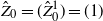 $\hat{Z}_0=(\hat{Z}_0^1)=(1)$
, and we have
$\hat{Z}_0=(\hat{Z}_0^1)=(1)$
, and we have $\ell(\hat Z_0)=1$
. As time passes, three different events may occur. First, a new individual may be born into the household counted by
$\ell(\hat Z_0)=1$
. As time passes, three different events may occur. First, a new individual may be born into the household counted by $\hat{Z}^1$
. Second, an individual in this household may pass away. The third possibility is that a new household, then counted by
$\hat{Z}^1$
. Second, an individual in this household may pass away. The third possibility is that a new household, then counted by $\hat{Z}^2$
, is formed. This happens according to a pure birth process
$\hat{Z}^2$
, is formed. This happens according to a pure birth process $\ell(\hat Z)$
with rate
$\ell(\hat Z)$
with rate $\lambda_1>0$
and independent of
$\lambda_1>0$
and independent of $\hat{Z}^1$
. Whichever event happens first, we label the random time it happens as
$\hat{Z}^1$
. Whichever event happens first, we label the random time it happens as $\hat{\sigma}_1$
. Now further births and deaths may happen in
$\hat{\sigma}_1$
. Now further births and deaths may happen in $\hat{Z}^1$
, and if it was already started, also in
$\hat{Z}^1$
, and if it was already started, also in $\hat{Z}^2$
. In addition, a new household with a single individual may be formed, counted by another independent copy of Z. We write
$\hat{Z}^2$
. In addition, a new household with a single individual may be formed, counted by another independent copy of Z. We write $\hat{\sigma}_2$
for the time that passes after
$\hat{\sigma}_2$
for the time that passes after $\hat{\tau}_1\,:\!=\,\hat{\sigma}_1$
until another birth, death, or independent formation of a new household occurs, and we set
$\hat{\tau}_1\,:\!=\,\hat{\sigma}_1$
until another birth, death, or independent formation of a new household occurs, and we set $\hat{\tau}_2\,:\!=\,\hat{\tau}_1+\hat{\sigma}_2$
. We now continue in a similar manner. This creates a sequence
$\hat{\tau}_2\,:\!=\,\hat{\tau}_1+\hat{\sigma}_2$
. We now continue in a similar manner. This creates a sequence $(\hat{\sigma}_k)_{k\in \mathbb{N}}$
of random times with partial sums
$(\hat{\sigma}_k)_{k\in \mathbb{N}}$
of random times with partial sums $\hat{\tau}_t=\sum_{k=1}^t \hat{\sigma}_k$
. We refer to the random times
$\hat{\tau}_t=\sum_{k=1}^t \hat{\sigma}_k$
. We refer to the random times $\hat{\tau}_t$
as census times; they form an increasing sequence
$\hat{\tau}_t$
as census times; they form an increasing sequence $(\hat{\tau}_t)_{t\in \mathbb{N}}$
. We write
$(\hat{\tau}_t)_{t\in \mathbb{N}}$
. We write $(\hat{\tau}^\ast_t)_{t\geq 1}$
for the subsequence of those census times at which a new houshold is formed, and we call them formation times. The households appear according to the pure birth process
$(\hat{\tau}^\ast_t)_{t\geq 1}$
for the subsequence of those census times at which a new houshold is formed, and we call them formation times. The households appear according to the pure birth process $\ell(\hat Z)$
and the formation times are exactly the successive jump times of this process. Consequently
$\ell(\hat Z)$
and the formation times are exactly the successive jump times of this process. Consequently $\hat{\tau}^\ast_1,\hat{\tau}^\ast_2-\hat{\tau}^\ast_1,\ldots,\hat{\tau}^\ast_{t}-\hat{\tau}^\ast_{t-1},\ldots$
are independent exponentially distributed random variables with parameters
$\hat{\tau}^\ast_1,\hat{\tau}^\ast_2-\hat{\tau}^\ast_1,\ldots,\hat{\tau}^\ast_{t}-\hat{\tau}^\ast_{t-1},\ldots$
are independent exponentially distributed random variables with parameters $\lambda_1,2\lambda_1,\ldots,t\lambda_1,\ldots$
, respectively. In the following, we assume that
$\lambda_1,2\lambda_1,\ldots,t\lambda_1,\ldots$
, respectively. In the following, we assume that $\hat Z=(\hat{Z}_u)_{u\geq 0}$
is defined on a probability space
$\hat Z=(\hat{Z}_u)_{u\geq 0}$
is defined on a probability space $(\hat{\Omega},\hat{\mathcal{F}},\hat{\mathbb{P}})$
. We provide a detailed construction in Appendix A.
$(\hat{\Omega},\hat{\mathcal{F}},\hat{\mathbb{P}})$
. We provide a detailed construction in Appendix A.
Since $\hat{\mathbb{P}}(\hat{\tau}_t\leq \hat{\tau}_{t+1}\colon t\in \mathbb{N}_0)=1$
by construction, and since the sequence of jump times
$\hat{\mathbb{P}}(\hat{\tau}_t\leq \hat{\tau}_{t+1}\colon t\in \mathbb{N}_0)=1$
by construction, and since the sequence of jump times $(\hat{\tau}^\ast_t)_{t\in \mathbb{N}_0}$
of the pure birth process
$(\hat{\tau}^\ast_t)_{t\in \mathbb{N}_0}$
of the pure birth process $\ell(\hat{Z})$
is a subsequence of
$\ell(\hat{Z})$
is a subsequence of $(\hat{\tau}_t)_{t\in\mathbb{N}_0}$
, we have
$(\hat{\tau}_t)_{t\in\mathbb{N}_0}$
, we have
 \begin{equation} \hat{\mathbb{P}}\Big(\lim_{t\to\infty}\hat{\tau}_t=+\infty\Big) = \hat{\mathbb{P}}\Big(\lim_{t\to\infty}\hat{\tau}_t^\ast=+\infty\Big) = 1.\end{equation}
5. An embedding and its consequences
We observe the following embedding of $\mathbf{d}$
into
$\mathbf{d}$
into $\hat{Z}$
.
$\hat{Z}$
.
Theorem 2. Let $\lambda_1,\lambda_2 > 0$
and
$\lambda_1,\lambda_2 > 0$
and $\mu_2\geq 0$
. Let
$\mu_2\geq 0$
. Let $\mathbf{d}=(\mathbf{d}_t)_{t\in\mathbb{N}_0}$
be the discrete-time Markov chain in (3), let
$\mathbf{d}=(\mathbf{d}_t)_{t\in\mathbb{N}_0}$
be the discrete-time Markov chain in (3), let $\hat Z=(\hat{Z}_u)_{u\geq 0}$
be the continuous-time S-valued process in (7), and let
$\hat Z=(\hat{Z}_u)_{u\geq 0}$
be the continuous-time S-valued process in (7), and let $(\hat{\tau}_t)_{t\in\mathbb{N}_0}$
be the associated sequence of census times. Then the processes
$(\hat{\tau}_t)_{t\in\mathbb{N}_0}$
be the associated sequence of census times. Then the processes $(\hat{Z}_{\hat{\tau}_t})_{t\in\mathbb{N}_0}$
and
$(\hat{Z}_{\hat{\tau}_t})_{t\in\mathbb{N}_0}$
and $(\mathbf{d}_t)_{t\in\mathbb{N}_0}$
have the same distribution.
$(\mathbf{d}_t)_{t\in\mathbb{N}_0}$
have the same distribution.
The arguments for the proof are standard; see, for instance, [Reference Athreya1, Theorem 3.3]. For the convenience of the reader we provide some comments in Appendix A.
Let $\hat Z=(\hat{Z}_u)_{u\geq 0}$
be the continuous-time S-valued process
$\hat Z=(\hat{Z}_u)_{u\geq 0}$
be the continuous-time S-valued process $\hat Z=(\hat{Z}_u)_{u\geq 0}$
in (7) with parameters
$\hat Z=(\hat{Z}_u)_{u\geq 0}$
in (7) with parameters $\lambda_1$
,
$\lambda_1$
, $\lambda_2$
, and
$\lambda_2$
, and $\mu_2$
. For any
$\mu_2$
. For any $u\geq 0$
, let
$u\geq 0$
, let $s(\hat{Z}_u)$
be the random variable on
$s(\hat{Z}_u)$
be the random variable on $(\hat{\Omega},\hat{\mathbb{P}},\hat{\mathcal{F}})$
fully determined by the set of conditional distributions
$(\hat{\Omega},\hat{\mathbb{P}},\hat{\mathcal{F}})$
fully determined by the set of conditional distributions
 \begin{equation} \hat{{\mathbb P}}\big(s(\hat{Z}_u)=j\mid \ell(\hat{Z}_u)=n\big) = \frac{1}{n}\sum_{i=1}^n\hat{{\mathbb P}}\big(\hat{Z}_u^i=j \mid \ell(\hat{Z}_u)=n\big),\quad n\in\mathbb{N}.\end{equation}
It may be interpreted as the size of a household chosen uniformly at random at time u. The next result is immediate from Theorem 2 and (8).
Corollary 1. Let $\lambda_1,\lambda_2>0$
and
$\lambda_1,\lambda_2>0$
and $\mu_2\geq 0$
. Given
$\mu_2\geq 0$
. Given $t\in \mathbb{N}_0$
and
$t\in \mathbb{N}_0$
and $u\geq 0$
, let
$u\geq 0$
, let $d(V_t)$
and
$d(V_t)$
and $s(\hat{Z}_u)$
be the random variables determined by (4) and (9), respectively. Then we have
$s(\hat{Z}_u)$
be the random variables determined by (4) and (9), respectively. Then we have $\mathbb{P}(d(V_t)= j)=$ $\hat{\mathbb{P}}(s(\hat{Z}_{\hat\tau_t})=j)$
for any
$\hat{\mathbb{P}}(s(\hat{Z}_{\hat\tau_t})=j)$
for any $t\in\mathbb{N}_0$
and
$t\in\mathbb{N}_0$
and $j\in\mathbb{N}_0$
, where
$j\in\mathbb{N}_0$
, where $(\hat{\tau}_t)_{t\in\mathbb{N}_0}$
is the sequence of census times associated with
$(\hat{\tau}_t)_{t\in\mathbb{N}_0}$
is the sequence of census times associated with $\hat{Z}$
. In particular,
$\hat{Z}$
. In particular,
 \begin{equation*} \lim_{t\rightarrow\infty}{\mathbb P}(d(V_t)= j) = \lim_{u\rightarrow\infty}\hat{{\mathbb P}}(s(\hat{Z}_u)= j),\quad j\in\mathbb{N}_0. \end{equation*}
Theorem 3 is a straightforward consequence of Theorem 2 and Corollary 1, together with [Reference Yule33] and the results in [21, Sections 2 and 3]. For the convenience of the reader we recall the known key facts from [Reference Lansky, Polito and Sacerdote21, Reference Yule33] in Appendix B, together with brief comments on (6).
Theorem 3. Let $\lambda_1,\lambda_2>0$
and
$\lambda_1,\lambda_2>0$
and $\mu_2\geq 0$
, let
$\mu_2\geq 0$
, let $\mathbf{d}$
be as in (3), and let
$\mathbf{d}$
be as in (3), and let $d(V_t)$
be the random variable determined by (4). Then the limits
$d(V_t)$
be the random variable determined by (4). Then the limits $p_j$
in (5) exist and are as follows:
$p_j$
in (5) exist and are as follows:
-
(i) If
$\mu_2=0$
, then (10)
\begin{equation} p_0=0, \qquad p_j=\frac{\lambda_1}{\lambda_2}\boldsymbol{B}\bigg(j,1+\frac{\lambda_1}{\lambda_2}\bigg),\quad j\in\mathbb{N}. \end{equation}
-
(ii) If
$\mu_2>0$
and
$\lambda_2>\mu_2$
, then (11)
\begin{align} p_0 & = \frac{\mu_2\lambda_1}{\lambda_2(\lambda_2-\mu_2)} \mathbf{B}\bigg(2,\frac{\lambda_1}{\lambda_2-\mu_2}\bigg) {}_2\mathbf{F}_1\bigg(1,\frac{\lambda_1}{\lambda_2-\mu_2},2+\frac{\lambda_1}{\lambda_2-\mu_2}, \frac{\mu_2}{\lambda_2}\bigg), \nonumber\\[-8pt] \end{align}
(12)
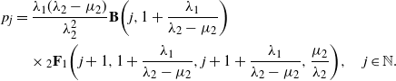
\begin{align} p_j & = \frac{\lambda_1(\lambda_2-\mu_2)}{\lambda_2^2} \mathbf{B}\bigg(j,1+\frac{\lambda_1}{\lambda_2-\mu_2}\bigg) \nonumber \\ & \quad \times {}_2\mathbf{F}_1\bigg(j+1,1+\frac{\lambda_1}{\lambda_2-\mu_2}, j+1+\frac{\lambda_1}{\lambda_2-\mu_2},\frac{\mu_2}{\lambda_2}\bigg), \quad j\in \mathbb{N}. \end{align}
-
(iii) If
$\mu_2>0$
and
$\lambda_2<\mu_2$
, then (13)
\begin{align} p_0 & = \frac{\lambda_1}{\mu_2-\lambda_2} \mathbf{B}\bigg(2,\frac{\lambda_1}{\mu_2-\lambda_2}\bigg) {}_2\mathbf{F}_1\bigg(1,\frac{\lambda_1}{\mu_2-\lambda_2},2+\frac{\lambda_1}{\mu_2-\lambda_2}, \frac{\lambda_2}{\mu_2}\bigg), \nonumber\\[-6pt]\end{align}
(14)
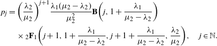
\begin{align} p_j & = \bigg(\frac{\lambda_2}{\mu_2}\bigg)^{j+1}\frac{\lambda_1(\mu_2-\lambda_2)}{\mu_2^2} \mathbf{B}\bigg(j,1+\frac{\lambda_1}{\mu_2-\lambda_2}\bigg) \nonumber \\ & \quad \times {}_2\mathbf{F}_1\bigg(j+1,1+\frac{\lambda_1}{\mu_2-\lambda_2}, j+1+\frac{\lambda_1}{\mu_2-\lambda_2},\frac{\lambda_2}{\mu_2}\bigg), \quad j\in \mathbb{N}. \end{align}
-
(iv) If
$\mu_2>0$
and
$\lambda_2=\mu_2$
, then (15)
\begin{equation} p_0 = \mathbf{U}\bigg(1,0,\frac{\lambda_1}{\lambda_2}\bigg), \qquad p_j = \frac{\lambda_1}{\lambda_2}\Gamma(j)\mathbf{U}\bigg(j,0,\frac{\lambda_1}{\lambda_2}\bigg), \quad j\in \mathbb{N}. \end{equation}









To obtain Theorem 1(i)–(iv) from Theorem 3 we can use known asymptotics for $\mathbf{B}$
,
$\mathbf{B}$
, ${}_2\mathbf{F}_1$
, and
${}_2\mathbf{F}_1$
, and $\mathbf{U}$
. For the convenience of the reader comments are provided in Appendix C.
$\mathbf{U}$
. For the convenience of the reader comments are provided in Appendix C.
Appendix A. Details on generalized Yule models and embeddings
A.1. A detailed construction of the generalized Yule model
Let $(\Omega',\mathcal{F}',\mathbb{P}')$
be the probability space over which the birth–death process
$(\Omega',\mathcal{F}',\mathbb{P}')$
be the probability space over which the birth–death process $Z=(Z_u)_{u\geq 0}$
is defined and such that
$Z=(Z_u)_{u\geq 0}$
is defined and such that $\mathbb{P}'(Z_0=1)=1$
. We consider the space
$\mathbb{P}'(Z_0=1)=1$
. We consider the space $(\hat{\Omega},\hat{\mathcal{F}},\hat{\mathbb{P}})$
, where
$(\hat{\Omega},\hat{\mathcal{F}},\hat{\mathbb{P}})$
, where

here, $\mathcal{E}_{k\lambda_1}$
denotes the exponential distribution with parameter
$\mathcal{E}_{k\lambda_1}$
denotes the exponential distribution with parameter $k\lambda_1>0$
. We use the notation
$k\lambda_1>0$
. We use the notation $(\omega,\pi)=((\omega_1,\omega_2,\ldots),(\pi_1,\pi_2,\ldots))$
with
$(\omega,\pi)=((\omega_1,\omega_2,\ldots),(\pi_1,\pi_2,\ldots))$
with $\omega_j\in \Omega'$
and
$\omega_j\in \Omega'$
and $\pi_k\in [0,+\infty)$
for the elements of
$\pi_k\in [0,+\infty)$
for the elements of $\hat{\Omega}$
. We now define
$\hat{\Omega}$
. We now define $\hat{Z}$
inductively.
$\hat{Z}$
inductively.
Let $\hat{Z}^1=(\hat{Z}^1_u)_{u\geq 0}$
be the process over
$\hat{Z}^1=(\hat{Z}^1_u)_{u\geq 0}$
be the process over $(\hat{\Omega},\hat{\mathcal{F}},\hat{\mathbb{P}})$
defined by
$(\hat{\Omega},\hat{\mathcal{F}},\hat{\mathbb{P}})$
defined by $\hat{Z}_u^1((\omega,\pi))\,:\!=\,Z_u(\omega_1), u\geq 0$
. It is convenient to set
$\hat{Z}_u^1((\omega,\pi))\,:\!=\,Z_u(\omega_1), u\geq 0$
. It is convenient to set $\hat{\sigma}_0\,:\!=\,0$
,
$\hat{\sigma}_0\,:\!=\,0$
, $\hat{\tau}_0\,:\!=\,0$
, and
$\hat{\tau}_0\,:\!=\,0$
, and $\hat{\tau}^\ast_0\,:\!=\,0$
.
$\hat{\tau}^\ast_0\,:\!=\,0$
.
We define the random times
 \begin{align*} \sigma_1^+(\hat{Z}^1) \,:\!=\, \inf\big\{u > 0\colon \hat{Z}_u^1=\hat{Z}_0^1+1\big\}, \qquad \sigma_1^-(\hat{Z}^1) \,:\!=\, \inf\big\{u>0\colon \hat{Z}_u^1=\hat{Z}_0^1-1\big\},\end{align*}
and $\sigma_1^\ast(\hat{Z})((\omega,\pi))\,:\!=\,\pi_{\ell(\hat{Z}_0)}=\pi_1$
; note that under
$\sigma_1^\ast(\hat{Z})((\omega,\pi))\,:\!=\,\pi_{\ell(\hat{Z}_0)}=\pi_1$
; note that under $\hat{\mathbb{P}}$
the time
$\hat{\mathbb{P}}$
the time $\sigma_1^\ast(\hat{Z})$
is independent of
$\sigma_1^\ast(\hat{Z})$
is independent of $\hat{Z}^1$
and exponentially distributed with parameter
$\hat{Z}^1$
and exponentially distributed with parameter $\lambda_1$
. We then set
$\lambda_1$
. We then set $\hat{\sigma}_1\,:\!=\,\min\big\{\sigma_1^+(\hat{Z}^1),\sigma_1^-(\hat{Z}^1),\sigma_1^\ast(\hat{Z})\big\}$
and
$\hat{\sigma}_1\,:\!=\,\min\big\{\sigma_1^+(\hat{Z}^1),\sigma_1^-(\hat{Z}^1),\sigma_1^\ast(\hat{Z})\big\}$
and $\hat{\tau}_1\,:\!=\,\hat{\sigma}_1$
, and define
$\hat{\tau}_1\,:\!=\,\hat{\sigma}_1$
, and define $\hat{Z}$
up to time
$\hat{Z}$
up to time $\hat{\tau}_1$
by
$\hat{\tau}_1$
by $\hat{Z}_u\,:\!=\,\big(\hat{Z}^1_u\big)$
,
$\hat{Z}_u\,:\!=\,\big(\hat{Z}^1_u\big)$
, $\hat{\tau}_0\leq u<\hat{\tau}_1$
.
$\hat{\tau}_0\leq u<\hat{\tau}_1$
.
If $\hat{\sigma}_1=\sigma_1^+(\hat{Z}^1)$
or
$\hat{\sigma}_1=\sigma_1^+(\hat{Z}^1)$
or $\hat{\sigma}_1=\sigma_1^-(\hat{Z}^1)$
, then we set
$\hat{\sigma}_1=\sigma_1^-(\hat{Z}^1)$
, then we set $\check{Z}_u^{(1)}\,:\!=\,\big(\hat{Z}_u^1\big)$
,
$\check{Z}_u^{(1)}\,:\!=\,\big(\hat{Z}_u^1\big)$
, $u\geq \hat{\tau}_1$
. If
$u\geq \hat{\tau}_1$
. If $\hat{\sigma}_1=\sigma_1^\ast(\hat{Z})$
, then we set
$\hat{\sigma}_1=\sigma_1^\ast(\hat{Z})$
, then we set $\hat{\tau}_1^\ast\,:\!=\,\hat{\tau}_1$
and
$\hat{\tau}_1^\ast\,:\!=\,\hat{\tau}_1$
and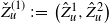 $\check{Z}_u^{(1)}\,:\!=\,\big(\hat{Z}_u^1,\hat{Z}^2_u\big)$
,
$\check{Z}_u^{(1)}\,:\!=\,\big(\hat{Z}_u^1,\hat{Z}^2_u\big)$
, $u\geq \hat{\tau}_1$
, where
$u\geq \hat{\tau}_1$
, where $\hat{Z}^2_u((\omega,\pi))\,:\!=\,Z_{u-\hat{\tau}_1^\ast}(\omega_2)$
,
$\hat{Z}^2_u((\omega,\pi))\,:\!=\,Z_{u-\hat{\tau}_1^\ast}(\omega_2)$
, $u\geq \hat{\tau}_1^\ast$
. The process
$u\geq \hat{\tau}_1^\ast$
. The process $\big(\check{Z}_u^{(1)}\big)_{u\geq \hat{\tau}_1}$
is a preliminary future version of
$\big(\check{Z}_u^{(1)}\big)_{u\geq \hat{\tau}_1}$
is a preliminary future version of $\hat{Z}$
starting at time
$\hat{Z}$
starting at time $\hat{\tau}_1$
.
$\hat{\tau}_1$
.
Now suppose that $t\in\mathbb{N}$
, the random time
$t\in\mathbb{N}$
, the random time $\hat{\tau}_t$
has been determined, and
$\hat{\tau}_t$
has been determined, and $\big(\check{Z}_u^{(t)}\big)_{u\geq \hat{\tau}_t}$
has been defined. The vector
$\big(\check{Z}_u^{(t)}\big)_{u\geq \hat{\tau}_t}$
has been defined. The vector $\check{Z}_{\hat{\tau}_t}^{(t)}$
has
$\check{Z}_{\hat{\tau}_t}^{(t)}$
has $\ell\big(\check{Z}_{\hat{\tau}_t}^{(t)}\big)$
components,
$\ell\big(\check{Z}_{\hat{\tau}_t}^{(t)}\big)$
components,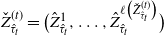 $\check{Z}_{\hat{\tau}_t}^{(t)}=\big(\hat{Z}^1_{\hat{\tau}_t}, \ldots, \hat{Z}^{\ell\big(\check{Z}_{\hat{\tau}_t}^{(t)}\big)}_{\hat{\tau}_t}\big)$
.
$\check{Z}_{\hat{\tau}_t}^{(t)}=\big(\hat{Z}^1_{\hat{\tau}_t}, \ldots, \hat{Z}^{\ell\big(\check{Z}_{\hat{\tau}_t}^{(t)}\big)}_{\hat{\tau}_t}\big)$
.
For any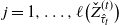 $j=1,\ldots,\ell\big(\check{Z}_{\hat{\tau}_t}^{(t)}\big)$
, define the random times
$j=1,\ldots,\ell\big(\check{Z}_{\hat{\tau}_t}^{(t)}\big)$
, define the random times
 \begin{align*} \hat{\sigma}_{t+1}^+(\hat{Z}^{\,j}) \,:\!=\, \inf\big\{u>0\colon\hat{Z}_{\hat{\tau}_t+u}^{\,j}=\hat{Z}_{\hat{\tau}_t}^{\,j}+1\big\},\qquad \hat{\sigma}_{t+1}^-(\hat{Z}^{\,j}) \,:\!=\, \inf\big\{u>0\colon\hat{Z}_{\hat{\tau}_t+u}^{\,j}=\hat{Z}_{\hat{\tau}_t}^{\,j}-1\big\},\end{align*}
and $\sigma^\ast_{t+1}(\hat{Z})((\omega,\pi))\,:\!=\,\pi_{\ell\big(\check{Z}_{\check{\tau}_t}^{(t)}\big)}.$
Under
$\sigma^\ast_{t+1}(\hat{Z})((\omega,\pi))\,:\!=\,\pi_{\ell\big(\check{Z}_{\check{\tau}_t}^{(t)}\big)}.$
Under $\hat{\mathbb{P}}$
the time
$\hat{\mathbb{P}}$
the time $\sigma^\ast_{t+1}(\hat{Z})$
is independent of
$\sigma^\ast_{t+1}(\hat{Z})$
is independent of $\big(\check{Z}_u^{(t)}\big)_{u\geq \hat{\tau}_t}$
and exponentially distributed with parameter
$\big(\check{Z}_u^{(t)}\big)_{u\geq \hat{\tau}_t}$
and exponentially distributed with parameter $\ell\big(\check{Z}_{\hat{\tau}_t}^{(t)}\big)\lambda_1$
. We set
$\ell\big(\check{Z}_{\hat{\tau}_t}^{(t)}\big)\lambda_1$
. We set
 \begin{align*} \hat{\sigma}_{t+1}\,:\!=\,\min\big\{\sigma_{t+1}^+(\hat{Z}^1), \ldots, \sigma_{t+1}^+\big(\hat{Z}^{\ell\big(\check{Z}_{\hat{\tau}_t}^{(t)}\big)}\big), \sigma_{t+1}^-(\hat{Z}^1), \ldots, \sigma_{t+1}^-\big(\hat{Z}^{\ell\big(\check{Z}_{\hat{\tau}_t}^{(t)}\big)}\big), \sigma_{t+1}^\ast(\hat{Z})\big\}\end{align*}
and $\hat{\tau}_{t+1}\,:\!=\,\sum_{k=1}^{t+1}\hat{\sigma}_k$
, and define
$\hat{\tau}_{t+1}\,:\!=\,\sum_{k=1}^{t+1}\hat{\sigma}_k$
, and define $\hat{Z}$
between time
$\hat{Z}$
between time $\hat{\tau}_t$
and
$\hat{\tau}_t$
and $\hat{\tau}_{t+1}$
by
$\hat{\tau}_{t+1}$
by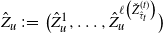 $\hat{Z}_u\,:\!=\,\big(\hat{Z}^1_u,\ldots,\hat{Z}^{\ell\big(\check{Z}_{\hat{\tau}_t}^{(t)}\big)}_u\big)$
,
$\hat{Z}_u\,:\!=\,\big(\hat{Z}^1_u,\ldots,\hat{Z}^{\ell\big(\check{Z}_{\hat{\tau}_t}^{(t)}\big)}_u\big)$
, $\hat{\tau}_t\leq u<\hat{\tau}_{t+1}$
.
$\hat{\tau}_t\leq u<\hat{\tau}_{t+1}$
.
If, for some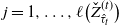 $j=1,\ldots,\ell\big(\check{Z}_{\hat{\tau}_t}^{(t)}\big)$
we have
$j=1,\ldots,\ell\big(\check{Z}_{\hat{\tau}_t}^{(t)}\big)$
we have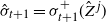 $\hat{\sigma}_{t+1}=\sigma_{t+1}^+(\hat{Z}^{\,j})$
or
$\hat{\sigma}_{t+1}=\sigma_{t+1}^+(\hat{Z}^{\,j})$
or $\hat{\sigma}_{t+1}=\sigma_{t+1}^-(\hat{Z}^{\,j})$
, then we set
$\hat{\sigma}_{t+1}=\sigma_{t+1}^-(\hat{Z}^{\,j})$
, then we set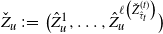 $\check{Z}_u\,:\!=\,\big(\hat{Z}^1_u,\ldots,\hat{Z}^{\ell\big(\check{Z}_{\hat{\tau}_t}^{(t)}\big)}_u\big)$
,
$\check{Z}_u\,:\!=\,\big(\hat{Z}^1_u,\ldots,\hat{Z}^{\ell\big(\check{Z}_{\hat{\tau}_t}^{(t)}\big)}_u\big)$
, $u\geq \hat{\tau}_{t+1}$
. If instead
$u\geq \hat{\tau}_{t+1}$
. If instead $\hat{\sigma}_{t+1}=\sigma_{t+1}^\ast(\hat{Z})$
, then we set
$\hat{\sigma}_{t+1}=\sigma_{t+1}^\ast(\hat{Z})$
, then we set $\hat{\tau}_{t+1}^\ast\,:\!=\,\hat{\tau}_{t+1}$
and
$\hat{\tau}_{t+1}^\ast\,:\!=\,\hat{\tau}_{t+1}$
and $\check{Z}_u\,:\!=\,\big(\hat{Z}^1_u,\ldots,\hat{Z}^{\ell\big(\check{Z}_{\hat{\tau}_t}^{(t)}\big)}_u, \hat{Z}^{\ell\big(\check{Z}_{\hat{\tau}_t}^{(t)}\big)+1}_u\big)$
,
$\check{Z}_u\,:\!=\,\big(\hat{Z}^1_u,\ldots,\hat{Z}^{\ell\big(\check{Z}_{\hat{\tau}_t}^{(t)}\big)}_u, \hat{Z}^{\ell\big(\check{Z}_{\hat{\tau}_t}^{(t)}\big)+1}_u\big)$
, $u\geq \hat{\tau}_{t+1}$
, where
$u\geq \hat{\tau}_{t+1}$
, where $\hat{Z}^{\ell\big(\check{Z}_{\hat{\tau}_t}^{(t)}\big)+1}_u((\omega,\pi))\,:\!=\,Z_{u-\hat{\tau}_{t+1}^\ast}(\omega_{t+2})$
,
$\hat{Z}^{\ell\big(\check{Z}_{\hat{\tau}_t}^{(t)}\big)+1}_u((\omega,\pi))\,:\!=\,Z_{u-\hat{\tau}_{t+1}^\ast}(\omega_{t+2})$
, $u\geq \hat{\tau}_{t+1}^\ast$
.
$u\geq \hat{\tau}_{t+1}^\ast$
.
Proceeding inductively, we now obtain the desired process $\hat Z=(\hat{Z}_u)_{u\geq 0}$
on
$\hat Z=(\hat{Z}_u)_{u\geq 0}$
on $(\hat{\Omega},\hat{\mathcal{F}},\hat{\mathbb{P}})$
.
$(\hat{\Omega},\hat{\mathcal{F}},\hat{\mathbb{P}})$
.
A.2. Comments on Theorem 2
Recall that if $Y_1,\ldots, Y_k$
are independent exponential random variables with parameters
$Y_1,\ldots, Y_k$
are independent exponential random variables with parameters $\delta_1,\ldots, \delta_k$
, then
$\delta_1,\ldots, \delta_k$
, then $\min(Y_1, Y_2,\ldots , Y_k)$
is exponentially distributed with parameter
$\min(Y_1, Y_2,\ldots , Y_k)$
is exponentially distributed with parameter $\delta_1+\cdots+\delta_k$
, and the probability that
$\delta_1+\cdots+\delta_k$
, and the probability that $\min(Y_1, Y_2,\ldots , Y_k)=Y_i$
is
$\min(Y_1, Y_2,\ldots , Y_k)=Y_i$
is $\delta_i\big(\sum_{j=1}^k \delta_j\big)^{-1}$
.
$\delta_i\big(\sum_{j=1}^k \delta_j\big)^{-1}$
.
Proof. Suppose that $n\in\mathbb{N}$
,
$n\in\mathbb{N}$
, ${\bf{x}}=(x_1,x_2,\ldots,x_n)\in S$
, and
${\bf{x}}=(x_1,x_2,\ldots,x_n)\in S$
, and $\hat{Z}_{\hat{\tau}_{t}}=\mathbf{x}$
. Stepping from
$\hat{Z}_{\hat{\tau}_{t}}=\mathbf{x}$
. Stepping from $\hat{\tau}_{t}$
to
$\hat{\tau}_{t}$
to $\hat{\tau}_{t+1}$
, a birth of an individual in household
$\hat{\tau}_{t+1}$
, a birth of an individual in household $\hat{Z}^i$
occurs with probability
$\hat{Z}^i$
occurs with probability
 \begin{align*} \hat{\mathbb{P}}\big(\hat{\sigma}_{t+1}=\sigma_{t+1}^+(\hat{Z}^i)\mid \hat{Z}_{\hat{\tau}_{t}}=\mathbf{x}\big) = \frac{x_i\lambda_2}{\sum_{j=1}^n(\lambda_2+\mu_2)x_j + n\lambda_1}, \end{align*}
a death of an individual in household $\hat{Z}^i$
with probability
$\hat{Z}^i$
with probability
 \begin{align*} \hat{\mathbb{P}}\big(\hat{\sigma}_{t+1}=\sigma_{t+1}^-(\hat{Z}^i)\mid\hat{Z}_{\hat{\tau}_{t}}=\mathbf{x}\big) = \frac{x_i\mu_2 }{\sum_{j=1}^n(\lambda_2+\mu_2)x_j + n\lambda_1}, \end{align*}
and the formation of a new household with probability
 \begin{align*} \hat{\mathbb{P}}\big(\hat{\sigma}_{t+1}=\sigma_{t+1}^\ast(\hat{Z})\mid\hat{Z}_{\hat{\tau}_{t}}=\mathbf{x}\big) = \frac{n\lambda_1}{\sum_{j=1}^n(\lambda_2+\mu_2)x_j + n\lambda_1}. \end{align*}
A comparison shows that these are exactly the transition probabilities of $\mathbf{d}$
in (3). In particular, the process
$\mathbf{d}$
in (3). In particular, the process $(\hat{Z}_{\hat{\tau}_t})_{t\in\mathbb{N}_0}$
is a discrete-time Markov chain with state space S. Since also
$(\hat{Z}_{\hat{\tau}_t})_{t\in\mathbb{N}_0}$
is a discrete-time Markov chain with state space S. Since also $\mathbf{d}_0=(1)=\hat{Z}_{\hat{\tau}_0}$
by construction, the Markov chains have the same distribution.
$\mathbf{d}_0=(1)=\hat{Z}_{\hat{\tau}_0}$
by construction, the Markov chains have the same distribution.
Appendix B. Some known key facts
The first fact was observed in [Reference Neuts and Resnick24, Theorem 1 and its proof]. Given $0\leq s_1\leq \cdots \leq s_n\leq u$
, we have
$0\leq s_1\leq \cdots \leq s_n\leq u$
, we have
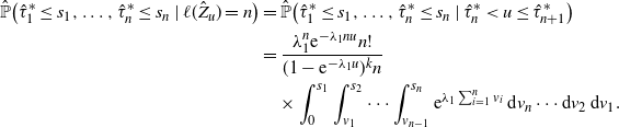 \begin{align} \hat{\mathbb{P}}\big(\hat{\tau}_1^\ast\leq s_1,\ldots,\hat{\tau}_n^\ast\leq s_n \mid \ell(\hat Z_u)=n\big) & = \hat{\mathbb{P}}\big(\hat{\tau}_1^\ast\leq s_1,\ldots,\hat{\tau}_n^\ast\leq s_n \mid \hat{\tau}^\ast_n < u\leq \hat{\tau}^\ast_{n+1}\big) \nonumber \\ & = \frac{\lambda_1^n{\mathrm{e}}^{-\lambda_1 nu}n!}{(1-{\mathrm{e}}^{-\lambda_1u})^kn} \nonumber \\ & \quad \times \int_0^{s_1}\int_{v_1}^{s_2}\cdots\int_{v_{n-1}}^{s_n}{\mathrm{e}}^{\lambda_1\sum_{i=1}^nv_i}\,{\mathrm{d}} v_n\cdots {\mathrm{d}} v_2\,{\mathrm{d}} v_1. \end{align}
The next fact was used in [Reference Lansky, Polito and Sacerdote21] and the sources quoted there. Suppose that $T_1,\ldots,T_n$
are independent [0,u]-valued random variables over some probability space with probability measure
$T_1,\ldots,T_n$
are independent [0,u]-valued random variables over some probability space with probability measure $\mathbb{Q}$
and all have the same density
$\mathbb{Q}$
and all have the same density $f_u(s)=\lambda_1{\mathrm{e}}^{\lambda_1 s}({\mathrm{e}}^{\lambda_1 u}-1)^{-1}$
,
$f_u(s)=\lambda_1{\mathrm{e}}^{\lambda_1 s}({\mathrm{e}}^{\lambda_1 u}-1)^{-1}$
, $0\leq s\leq u$
.
$0\leq s\leq u$
.
Now let $T_{(1)},\ldots,T_{(n)}$
denote their order statistics. Then
$T_{(1)},\ldots,T_{(n)}$
denote their order statistics. Then $\mathbb{Q}(T_{(1)}\leq s_1,\ldots,T_{(n)}\leq s_n)$
equals (16). Consequently, given
$\mathbb{Q}(T_{(1)}\leq s_1,\ldots,T_{(n)}\leq s_n)$
equals (16). Consequently, given $0\leq s\leq u$
, we have
$0\leq s\leq u$
, we have
 \begin{align*} \frac{1}{n}\sum_{j=1}^n\hat{\mathbb{P}}\big(\hat{\tau}^\ast_j\leq s\mid \ell(\hat Z_u)=n\big) = \frac{1}{n}\sum_{j=1}^n\mathbb{Q}(T_{(j)}\leq s)=\mathbb{Q}(T_1\leq s).\end{align*}
That is, $f_u$
is the density of the formation time of a household chosen with uniform probability among all the households existing at time u. Consequently, using the Markov property of the birth–death process
$f_u$
is the density of the formation time of a household chosen with uniform probability among all the households existing at time u. Consequently, using the Markov property of the birth–death process $Z=(Z_u)_{u\geq 0}$
starting at one over
$Z=(Z_u)_{u\geq 0}$
starting at one over $(\Omega',\mathcal{F}',\mathbb{P}')$
,
$(\Omega',\mathcal{F}',\mathbb{P}')$
,
 \begin{align} p_j = \lim_{u\rightarrow\infty}\hat{\mathbb{P}}\big(s(\hat{Z}_u)=j\big) & = \lim_{u\rightarrow\infty}\int_{0}^{u}\mathbb{P}'\big(Z_{u-s}=j \mid Z_s=1\big)f_u(s)\,{\mathrm{d}} s \nonumber \\ & = \lim_{u\rightarrow\infty}\frac{\lambda_1}{1-{\mathrm{e}}^{-\lambda_1 u}}\int_{0}^{u}{\mathrm{e}}^{-\lambda_1 v}\mathbb{P}'(Z_{v}=j)\,{\mathrm{d}} v \nonumber \\ & = \lambda_1\int_{0}^{\infty}{\mathrm{e}}^{-\lambda_1 v}\mathbb{P}'(Z_{v}=j)\,{\mathrm{d}} v, \quad j\in\mathbb{N}_0. \end{align}
For the pure birth case $\mu_2=0$
, we can now use the classical fact that
$\mu_2=0$
, we can now use the classical fact that $\mathbb{P}'(Z_{v}=0)=0$
and
$\mathbb{P}'(Z_{v}=0)=0$
and $\mathbb{P}'(Z_{v}=j)={\mathrm{e}}^{-\lambda_2 v}(1-{\mathrm{e}}^{-\lambda_2 v})^{j-1}$
,
$\mathbb{P}'(Z_{v}=j)={\mathrm{e}}^{-\lambda_2 v}(1-{\mathrm{e}}^{-\lambda_2 v})^{j-1}$
, $j\in \mathbb{N}$
(see, for instance, [Reference Bailey3, Chapter 8]). This gives the well-known expression (10) in terms of
$j\in \mathbb{N}$
(see, for instance, [Reference Bailey3, Chapter 8]). This gives the well-known expression (10) in terms of $\mathbf{B}$
, cf. [Reference Lansky, Polito and Sacerdote21, Section 2] or [Reference Yule33]. Now suppose that
$\mathbf{B}$
, cf. [Reference Lansky, Polito and Sacerdote21, Section 2] or [Reference Yule33]. Now suppose that $\mu_2>0$
. In the super- and subcritical cases we can use the known fact that
$\mu_2>0$
. In the super- and subcritical cases we can use the known fact that
 \begin{align*} \mathbb{P}'(Z_{v}=0) & = \frac{\mu_2(1-{\mathrm{e}}^{(\lambda_2-\mu_2)u})}{\lambda_2-\mu_2{\mathrm{e}}^{-(\lambda_2-\mu_2)u}}, \\ \mathbb{P}'(Z_{v}=j) & = (\lambda_2-\mu_2)^2{\mathrm{e}}^{-(\lambda_2-\mu_2)u}\frac{\lambda_2^{j-1}(1-{\mathrm{e}}^{-(\lambda_2-\mu_2)u})^{j-1}}{(\lambda_2-\mu_2{\mathrm{e}}^{-(\lambda_2-\mu_2)u})^{j+1}}, \quad j\in \mathbb{N};\end{align*}
see [Reference Bailey3, Chapter 8]. Plugging these expressions into (17), we can rewrite the result in terms of ${}_2\mathbf{F}_1$
to obtain (11), (12), (13), and (14). This was observed in [Reference Lansky, Polito and Sacerdote21, Section 3.2]. In the critical case we can use
${}_2\mathbf{F}_1$
to obtain (11), (12), (13), and (14). This was observed in [Reference Lansky, Polito and Sacerdote21, Section 3.2]. In the critical case we can use
 \begin{align*} \mathbb{P}'(Z_{v}=0) = \frac{\lambda_2 u}{1+\lambda_2 u}, \qquad \mathbb{P}'(Z_{v}=j) = \frac{(\lambda_2 u)^{j-1}}{(1+\lambda_2 u)^{j+1}}, \quad j\in \mathbb{N},\end{align*}
[Reference Bailey3, Chapter 8]. Plugging into (17), we obtain (15), as found in [Reference Lansky, Polito and Sacerdote21, Section 3.1].
To see (6), let $\mathbb{E}'$
denote the expectation with respect to
$\mathbb{E}'$
denote the expectation with respect to $\mathbb{P}'$
and note that Fubini and (17) give
$\mathbb{P}'$
and note that Fubini and (17) give
 \begin{align*} \mathbb{E}[d(V_\infty)] = \sum_{j=0}^\infty jp_j = \lambda_1\int_0^\infty{\mathrm{e}}^{-\lambda_1 v}\sum_{j=0}^\infty j\mathbb{P}'(Z_v=j)\,{\mathrm{d}} v = \lambda_1\int_0^\infty{\mathrm{e}}^{-\lambda_1 v}\mathbb{E}'[Z_v]\,{\mathrm{d}} v.\end{align*}
Now it suffices to take into account the known fact that
 \begin{align*} {\mathbb E}'(Z_v) = \begin{cases} {\mathrm{e}}^{(\lambda_2-\mu_2)v}, & \lambda_2\neq \mu_2, \\ 1, & \lambda_2= \mu_2; \end{cases}\end{align*}
see [Reference Bailey3, Chapter 8].
Remark 2. In a similar manner we can calculate the variance $\mathbb{V}[d(V_\infty)]$
of a random variable
$\mathbb{V}[d(V_\infty)]$
of a random variable $d(V_\infty)$
with distribution
$d(V_\infty)$
with distribution $(p_j)_{j\geq 0}$
. This gives
$(p_j)_{j\geq 0}$
. This gives
 \begin{align*} & \mathbb{V}[d(V_\infty)] \\ & = \begin{cases} \dfrac{\frac{2\lambda_1\lambda_2}{\lambda_1-2(\lambda_2-\mu_2)}-\frac{\lambda_1(\lambda_2+\mu_2)} {\lambda_1-(\lambda_2-\mu_2)}}{\lambda_2-\mu_2} - \bigg(\dfrac{\lambda_1}{\lambda_1-(\lambda_2-\mu_2)}\bigg)^2 & \text{if } \mu_2>\lambda_2 \text{ or } \lambda_2-2\lambda_1<\mu_2 <\lambda_2, \\ 2\bigg(\dfrac{\lambda_2}{\lambda_1}\bigg) & \text{if } \lambda_2=\mu_2, \\ \infty & \text{otherwise}. \end{cases} \end{align*}
Appendix C. Large-parameter asymptotics
For fixed $b>0$
we have
$b>0$
we have $\mathbf{B}(j,b)\sim \Gamma(b)j^{-b}$
as
$\mathbf{B}(j,b)\sim \Gamma(b)j^{-b}$
as $j\to \infty$
. Combined with Theorem 3(i) this gives Theorem 1(i).
$j\to \infty$
. Combined with Theorem 3(i) this gives Theorem 1(i).
To obtain the asymptotics in Theorem 1(ii) and (iii) from (12) and (14), respectively, note that for any $b>0$
,
$b>0$
, $\gamma>0$
, and
$\gamma>0$
, and $0<z<1$
, we have
$0<z<1$
, we have
 \begin{align*}{}_2\mathbf{F}_1(j+1,b,j+1+\gamma,z)={}_2\mathbf{F}_1(b, j+1,j+1+\gamma,z)\sim (1-z)^{-b};\end{align*}
see [Reference Temme30, Section 2].
To see Theorem 1(iv) we use the fact that for any $z>0$
there is a function R(j) of j and a constant
$z>0$
there is a function R(j) of j and a constant $C>0$
such that
$C>0$
such that $\limsup_{j\to\infty} R(j) < C$
and
$\limsup_{j\to\infty} R(j) < C$
and
 \begin{equation} \Gamma(j)\mathbf{U}(j,0,z) = 2{\mathrm{e}}^{{z}/{2}}\bigg(\sqrt{2\beta\tanh\bigg(\frac{w}{2}\bigg)}K_1(2j\beta) + \frac{({1}/{j})+\beta}{j+j\beta}{\mathrm{e}}^{-2j\beta}R(j)\bigg);\end{equation}
here, $w=w(j)$
and
$w=w(j)$
and $\beta=\beta(j)$
are given by
$\beta=\beta(j)$
are given by $w(j)=\cosh^{-1}(1+{z}/{2j})$
and
$w(j)=\cosh^{-1}(1+{z}/{2j})$
and $\beta(j)=\frac12(w(j)+\sinh(w(j)))$
, and
$\beta(j)=\frac12(w(j)+\sinh(w(j)))$
, and $K_1$
denotes the modified Bessel function of the second kind of order one; see [Reference Olver, Daalhuis, Lozier, Schneider, Boisvert, Clark, Miller, Saunders, Cohl and McClain26, 13.8(iii)]. Since
$K_1$
denotes the modified Bessel function of the second kind of order one; see [Reference Olver, Daalhuis, Lozier, Schneider, Boisvert, Clark, Miller, Saunders, Cohl and McClain26, 13.8(iii)]. Since $w(j)\sim ({z}/{2j})+\sqrt{(1+{z}/{2j})^2-1}$
and
$w(j)\sim ({z}/{2j})+\sqrt{(1+{z}/{2j})^2-1}$
and $\beta(j)\sim w(j)$
, we find that
$\beta(j)\sim w(j)$
, we find that
 \begin{equation} 2j\beta(j)\sim z+2\sqrt{jz+\frac{z^2}{4}}\sim 2\sqrt{jz}, \qquad \frac{\beta(j)}{j}\sim \frac{\sqrt{z}}{j^{3/2}}.\end{equation}
The known asymptotics for $K_1$
gives
$K_1$
gives
 \begin{align*}K_1(2j\beta(j))\sim \sqrt{\frac{\pi}{4 j\beta(j)}}{\mathrm{e}}^{-2j\beta(j)};\end{align*}
see [Reference Olver, Daalhuis, Lozier, Schneider, Boisvert, Clark, Miller, Saunders, Cohl and McClain26, 10.25(ii)]. Consequently the first summand in brackets on the right-hand side of (18) behaves like
 \begin{align*}\sim \beta(j)K_1(2j\beta(j))\sim \frac{\sqrt{\pi}}{2}\sqrt{\frac{\beta(j)}{j}}{\mathrm{e}}^{-2j\beta(j)}.\end{align*}
Given $m\in \mathbb{N}$
we have
$m\in \mathbb{N}$
we have $j^m{\mathrm{e}}^{-2j\beta(j)} < j^m(2j\beta(j))^{-2m}\leq z^{-m}$
for all large enough j by the first part in (19). Using also the second part we see that
$j^m{\mathrm{e}}^{-2j\beta(j)} < j^m(2j\beta(j))^{-2m}\leq z^{-m}$
for all large enough j by the first part in (19). Using also the second part we see that $j^m \beta(j)K_1(2j\beta(j))\to 0$
. For any
$j^m \beta(j)K_1(2j\beta(j))\to 0$
. For any $\varepsilon>0$
we eventually have
$\varepsilon>0$
we eventually have ${\mathrm{e}}^{\varepsilon j}{\mathrm{e}}^{-2j\beta(j)}<{\mathrm{e}}^{\frac{\varepsilon}{2}j}$
, and therefore
${\mathrm{e}}^{\varepsilon j}{\mathrm{e}}^{-2j\beta(j)}<{\mathrm{e}}^{\frac{\varepsilon}{2}j}$
, and therefore ${\mathrm{e}}^{\varepsilon j}\beta(j)K_1(2j\beta(j))\to +\infty$
. The second summand in parentheses on the right-hand side of (18) behaves similarly.
${\mathrm{e}}^{\varepsilon j}\beta(j)K_1(2j\beta(j))\to +\infty$
. The second summand in parentheses on the right-hand side of (18) behaves similarly.
Acknowledgements
We thank the anonymous referee for various suggestions that helped us to improve the text.
Funding information
There are no funding bodies to thank relating to the creation of this article.
Competing interests
There were no competing interests to declare which arose during the preparation or publication process of this article.

 Open access

