1.1. Models of the space–time spectrum of turbulence

Kraichnan (Reference Kraichnan1964) and Lumley (Reference Lumley1965) both proposed a model spectrum of turbulence in which small-scale turbulent fluctuations, $u$, were convected by a spatially and temporally uniform fluctuating field, $v$, in addition to some mean velocity, $U$. Lumley found that the width of the resulting frequency spectrum, as measured by its normalized second moment, was described by the magnitude of fluctuations of the convective velocity, $\langle v^2 \rangle$, divided by their corresponding Taylor microscale. Therefore, the observed broadening of the energy spectrum was indicative of variations in instantaneous convection velocities about the mean convection velocity predicted by Taylor's hypothesis. Kraichnan utilized this same scalar convection model of turbulence to study the more general validity of Kolmogorov's assumption that large and small scales are statistically independent when sufficiently separated. Since Kraichnan's work, this convection model has been referred to as the ‘random-sweeping hypothesis’, since the large scale, $v$, was assumed to sweep the turbulence along as a passive scalar.

The random-sweeping model was extended by Wilczek & Narita (Reference Wilczek and Narita2012) to obtain an analytical expression for the frequency–wavenumber spectrum, in which the mean convection velocity was represented by Taylor's hypothesis and the width of the spectrum in the frequency domain was found to scale with the magnitude of fluctuations of the convective velocity, $\langle v^2 \rangle$, consistent with Lumley. They also showed that their model was consistent with predictions from an alternative, elliptic approximation model (He & Zhang Reference He and Zhang2006; He, Jin & Yang Reference He, Jin and Yang2017). Wilczek, Stevens & Meneveau (Reference Wilczek, Stevens and Meneveau2015b) later applied this analytical spectral model to the case of wall-bounded flows by using the Townsend's log law for the Reynolds stresses to represent the turbulence intensity associated with the spectral width (Marusic et al. Reference Marusic, Monty, Hultmark and Smits2013). They reported good qualitative agreement between the analytical frequency–wavenumber spectrum and that obtained via large eddy simulations (LES), although some deviations were apparent.

Importantly, Wilczek et al. (Reference Wilczek, Stevens, Narita and Meneveau2014) noted that the true spectral width (in the frequency domain) is non-zero when approaching the smallest wavenumbers, and yet the one-dimensional (1-D) random-sweeping model predicted zero width in this limit. They attributed this discrepancy to two possible sources: the neglect of scale interactions at the large scales of turbulence and the lack of influence from spanwise wavenumbers. Later, Wilczek, Stevens & Meneveau (Reference Wilczek, Stevens and Meneveau2015a) extended the 1-D sweeping model to include spanwise wavenumbers and showed how this appeared to resolve the low-wavenumber singularity, but they did not provide a quantitative comparison of spectral width variation with wavenumbers, and they left open the question of the influence of scale interactions.

Liu & Gayme (Reference Liu and Gayme2020) proposed an alternative approach to calculating the distribution of convection velocities based on a linearized, input–output model of turbulent channel flow, and they estimated power-spectral densities as a function of convection velocity, where the width of the power spectrum was shown to narrow for smaller scales and was found to be roughly symmetric about the mean convection velocity (except for certain intermediate-sized scales), largely consistent with the sweeping model predictions. However, they also did not report quantitative comparisons of spectral width with respect to wavenumber, and their linear analysis necessarily neglected the influence of scale interactions.

There are a number of analytical tools available for describing and reconstructing the width of the space–time spectrum, most of which appear in the important study by Beall, Kim & Powers (Reference Beall, Kim and Powers1982). If we denote the turbulent spectral density of the streamwise velocity component, $u$, with streamwise wavenumber, $k_x$, and frequency, $\omega$, as $\phi _{uu}(k_x,\omega )$, then Beall et al. (Reference Beall, Kim and Powers1982) introduced the idea of a ‘conditional spectral density’, $\phi _{uu}(\omega | k_x)$, as the normalized spectrum

(1.1)\begin{equation} \phi_{uu}(\omega | k_x) = \frac{\phi_{uu}(k_x,\omega)}{\int_{-\infty}^{\infty} \phi_{uu}(k_x,\omega) \, {\rm d}\omega}, \end{equation}

such that $\phi _{uu}(\omega | k_x) \Delta \omega$ represents the fraction of power at $k_x$ due to fluctuations between $(\omega,\omega +\Delta \omega )$ and is analogous to a conditional probability. This means that the conditional spectral density can be interpreted naturally as a probability density function (p.d.f.), and according to the model of Wilczek & Narita (Reference Wilczek and Narita2012), that p.d.f. is predicted to be a normal distribution. (The results of Liu & Gayme (Reference Liu and Gayme2020) show some non-Gaussian spectral distributions for intermediate $k_x$ scales, but Wilczek et al. (Reference Wilczek, Stevens and Meneveau2015a) found that the Gaussian behaviour was largely maintained even for anisotropic, wall-bounded flows.) As a consequence, the conditional spectral density can be used directly to determine the spectral width by integrating its second moment (variance) directly, as discussed in Narita (Reference Narita2017).

Because the spectral width in the frequency domain, $\omega$, can be transformed into a spectral width in the phase-speed domain, $c$, for a fixed wavenumber, where $c = \omega /k_x$, the spectral width provides a direct measure of the variability of the turbulent energy across phase speeds, which is a natural way of thinking about the sweeping model described above, where the variance of the analytical spectrum was found to depend on the variance of the large-scale velocity signal, $\langle v^2 \rangle$.

In addition to the direct measurement of the spectral moments from the space–time spectrum, Beall et al. (Reference Beall, Kim and Powers1982) also showed that the spectral moments can be inferred from the joint p.d.f. of the auto-spectral energy and local frequencies (or wavenumbers) that are defined via the cross-spectrum. This technique allows for the reconstruction of the space–time spectrum with limited two-point measurements in either one of the dimensions, a technique that was later employed by De Kat & Ganapathisubramani (Reference De Kat and Ganapathisubramani2015). Furthermore, Beall et al. (Reference Beall, Kim and Powers1982) showed that the spectral variance calculated from the joint p.d.f. is expected to differ from the direct integration of the spectral moment by an amplitude-dependent term – this result was later emphasized by Wu et al. (Reference Wu, Geng, Yao, Xu and He2017) who empirically compensated for the discrepancy in their spectral models (see their review of these topics in Wu & He Reference Wu and He2021a). However, all of these techniques for quantifying the spectral width must be applied with care, in particular, accounting for the limitations of experiments, which have mostly focused on establishing a mean convection velocity and not its variance.

1.2. Measurement and quantification of convection velocities

A significant number of experimental studies have sought to measure the mean convection velocities of coherent structures in turbulence, from the early studies of Cliff & Sandborn (Reference Cliff and Sandborn1973) and later Kim & Hussain (Reference Kim and Hussain1992), to more recent efforts to measure the space–time spectrum directly with particle image velocimetry (PIV) by Dennis & Nickels (Reference Dennis and Nickels2008), Elsinga et al. (Reference Elsinga, Poelma, Schrãder, Geisler, Scarano and Westerweel2012) and LeHew, Guala & McKeon (Reference LeHew, Guala and McKeon2011). The key computational study by Del Álamo & Jiménez (Reference Del Álamo and Jiménez2009) summarized many of the challenges in defining a single characteristic convection velocity for each wavenumber or frequency, given the width of the space–time spectrum in both dimensions, and they proposed weighted-integral approaches to answer this question consistently. Some physical insights into this problem from a transport perspective were later offered by Geng et al. (Reference Geng, He, Wang, Xu, Lozano-Durán and Wallace2015). A comprehensive study of the convection velocity, based on an LES calculation at ${Re}_\theta = 13\,000$ was performed by Renard & Deck (Reference Renard and Deck2015), who also reviewed and tabulated all the previous measurements and calculation techniques.

Despite the extensive studies involving wavenumber–frequency spectra, there are very few reports of the wavenumber dependence of the frequency spectrum variance. Direct numerical simulation (DNS) channel flow calculations of the spectral variance at ${Re}_\tau = 187$ (Yang et al. Reference Yang, Jin, Wu, Yang and He2020) and ${Re}_\tau = 550$ (Wu & He Reference Wu and He2021b) have been reported, although they enforced Taylor's hypothesis in their definition of the second spectral moment, and their Reynolds numbers were relatively low.

1.3. Convection velocities and the inclination angles of coherent structures

Like the interest in the scale dependence of convection velocities, there has been similar interest in the scale dependence of coherent structure inclination angles. Deshpande, Monty & Marusic (Reference Deshpande, Monty and Marusic2019) reported inclination angle variation as a function of streamwise wavelength for different spanwise scale sizes, and validated the traditionally assumed inclination angle of $45^\circ$ for individual, large-scale, wall-attached structures (as opposed to the $15^\circ$ for overall packets). Li et al. (Reference Li, Hutchins, Zheng, Marusic and Baars2022) examined the same scale dependence of inclination angles in the atmospheric surface layer under both unstable and neutrally stable conditions. Following Chauhan et al. (Reference Chauhan, Hutchins, Monty and Marusic2013), they developed a log-law-type empirical formula to relate the inclination angle and structure wavelength.

A few studies have looked at how structure geometry and scale-specific convection velocity are related. LeHew, Guala & McKeon (Reference LeHew, Guala and McKeon2013) examined the connection between the convection velocity of vortices and whether they were attached to the wall and found a higher variance in the convection velocity for attached structures. Lozano-Durán & Jiménez (Reference Lozano-Durán and Jiménez2014) performed a similar analysis, computationally. More recently, Huang (Reference Huang2019) developed a model to relate the mean velocity profile to the inclination angles of coherent structures by utilizing an expression for the variance of velocity fluctuations for an individual eddy by Banerjee & Katul (Reference Banerjee and Katul2013). They confirmed that the inclination angle can be used to improve predictions of the mean velocity profile, via comparison with DNS profiles, although they did not explore the indirect dependence of their model on the local convection velocity variance, which would require detailed measurements of the local, scale-dependent convection velocities of the eddies. The relationship between scale-specific convection velocity and inclination angle of coherent structures also arises in the context of resolvent-based modelling of turbulence, in which the phase velocity of modes dictates the mode shape, including its relative inclination to the wall (see McKeon (Reference McKeon2017) for an overview and Cui & Jacobi (Reference Cui and Jacobi2023) for specific observations on inclination angles).

In this study we performed experimental measurements of a turbulent boundary layer to obtain the scale-dependent variance of phase speeds and to examine its relationship to the scale-dependent inclination angles of coherent structures in the flow. The experiments are described in § 2. In § 3 we report the spectral variance of phase speed as a function of streamwise and spanwise wavenumbers and identify persistent discrepancies with previous versions of the random-sweeping model. We extend the random-sweeping model of turbulence (under simplifying assumptions) to include 1-D scale interactions in order to explain the dominant streamwise-wavenumber dependence of variance for large-scale motions (LSMs). Then, in § 4 we explore the relations between structure size, inclination angle and phase speed, using space–time cross-spectral analysis, in order to develop intuition about how variations in phase speed are associated with the average inclination angles of velocity modes, the size of the modes and the strength of the mean shear of the flow field.

3.1. Space–time spectral density

The 2-D space–time spectral energy density with respect to streamwise wavenumber, $k_x$, and frequency, $\omega$, was calculated from the 2-D fast Fourier transform (FFT) of the fluctuating velocity for each height from the streamwise/wall-normal measurements. Each of the continuous time series was segmented by Welch's method with a temporal segment size selected to be comparable to the spatial domain size of the FOV. The mean was removed and Hanning windows were applied to both the streamwise spatial and temporal segments. The data was zero padded, and the FFT was calculated with 50 % overlap between the segments, all following the procedure in LeHew et al. (Reference LeHew, Guala and McKeon2011) with the exception of mean removal, where they removed the global mean and we removed the segment mean. The effect of the choice of mean removal on the energy of LSMs is explored in detail in Appendix A.

The $k_x/\omega$ spectrum is shown in figure 2(a), where the slope of the solid red line indicates the convective velocity associated with Taylor's hypothesis and the dashed cyan line indicates the frequency-weighted average velocity obtained from the first spectral moment (Jiménez, Del Alamo & Flores Reference Jiménez, Del Alamo and Flores2004; Flores & Jimenez Reference Flores and Jimenez2006). The black contour line marks the isocontour of spectral energy density that contains within it 30 % of the total streamwise turbulent kinetic energy (TKE), $\overline {u'^2}$. This constant energy fraction contour was used to observe trends in the spectral distribution of the streamwise TKE as a function of wall-normal height, shown in figure 2(b) and as a function of Reynolds number, shown in figure 2(c). For validation, the space–time spectral density from the wall-parallel plane at this height (not shown), integrated over all spanwise wavenumbers, $k_z$, was found to match the spectrum obtained from the streamwise/wall-normal measurements.

Figure 2.

(a) Space–time spectral energy density, $\phi _{uu}(k_x,\omega )$ at $y/\delta \approx 0.1$ for ${Re}_\tau =3070$. The local mean velocity (Taylor's hypothesis) is marked in red; the average convection velocity (Jiménez et al. Reference Jiménez, Del Alamo and Flores2004) is marked in dashed cyan. The isocontour of spectral energy containing 30 % of the streamwise TKE is in black. (b) The 30 % energy fraction contours for varying wall-normal locations, $y/\delta \approx 0.04, 0.1, 0.5$ (darker lines at higher $y$), at fixed ${Re}_\tau =3070$. (c) The energy fraction contours for varying ${Re}_\tau$ (darker lines at higher ${Re}_\tau$) at $y/\delta \approx 0.1$.

As the wall-normal position increases, the energy fraction contour expands to include more small-scale, high frequency content (beyond the wall-normal location of the outer LSM peak). The large-scale, low frequency region of the contour also shifts slightly to larger, faster coherent motions appearing further away from the wall. For a fixed wall-normal location (in outer units), increasing the Reynolds number results in a contraction of the energy contour, indicating increased domination of the flow by large-scale coherent motions. But ultimately, the Reynolds numbers effects on the large scales are rather weak over this range, as noted in the subsequent analysis.

Previous studies (Jiménez et al. Reference Jiménez, Del Alamo and Flores2004; Flores & Jimenez Reference Flores and Jimenez2006; LeHew et al. Reference LeHew, Guala and McKeon2011) have focused on the fact that the weighted-average convective velocity, marked as the cyan line in figure 2(a), does not have a constant slope, as Taylor's hypothesis would dictate (red line), but varies with wavenumber, with the greatest deviation for the large scales near the wall. However, in addition to the variation of the weighted average frequency with wavenumber, figure 2(a) also shows a significant variation in the width of the frequency spectrum with wavenumber. The width of the frequency spectrum for a given wavenumber can be thought of in terms of the phase velocity variation, since $c = \omega /k_x$, and thus represents the distribution of energy across different phase velocities associated with velocity modes of that particular wavenumber. Based on this, variations in the width of the space–time spectrum with wavenumber indicate that the distribution of convective velocities is strongly size dependent. However, from figure 2(b,c), it is clear that the distribution of convective velocities (the width of the $\omega$-spectral density) varies only weakly with wall-normal location, $y$, and ${Re}_\tau$. However, stronger y variation is expected in the near wall region below the log layer that was not resolved in the experimental measurements.

3.2. Conditional wavenumber spectrum and convection velocity variance

In order to quantify the changing distribution of convective velocities with structure size, we first transform the frequency, $\omega$, of the 2-D spectrum, $\phi _{uu}(k_x,\omega )$, into phase speed $c$, via the relation $c = \omega /k_x$, to obtain $\phi _{uu}(k_x,c)$. Then we employ the conditional wavenumber spectral density described by Beall et al. (Reference Beall, Kim and Powers1982) to calculate the p.d.f. of phase speeds for each wavenumber, $\phi _{uu}(c|k_x)$. The conditional spectrum provides a spectral view on the relative distribution of phase speeds associated with the coherent structures in the boundary layer. The distribution of phase speeds is here taken as representative of the distribution of convective velocities, and the terms will be used interchangeably, forgiving the slight imprecision involved. Similarly, the mode shapes associated with individual wavenumbers are assumed to characterize the typical coherent structure of the corresponding scale, although in reality coherent structures contain spectral energy content from a range of wavenumbers.

For calculating conditional spectral density, it is important to remove the noise floor of the spectrum due to the PIV measurements first, in order not to contaminate the shape of the resulting p.d.f. by the appearance of spurious distribution tails that are actually just noise. This baseline subtraction was based on the power calculated at the Nyquist frequency, following Oxlade et al. (Reference Oxlade, Valente, Ganapathisubramani and Morrison2012). The resulting conditional spectrum is shown in figure 3. The wavenumber dependence of the width of the convective velocity distribution is quite prominent, particularly for the large scales, $k_x \delta \lesssim 2 {\rm \pi}$. Past a wavenumber of $k_x \delta \gtrsim 25$, the signal-to-noise (SNR) ratio – defined as the ratio between the spectral peak and noise floor – dips below $10$. Thus, the noise floor becomes so large relative to the turbulent spectral energy that the distribution becomes noticeably truncated for these high wavenumbers.

Figure 3.

The conditional wavenumber spectrum, $\phi _{uu}(c|k_x)$, following Beall et al. (Reference Beall, Kim and Powers1982), but in terms of the deviation of the phase speed, $c$, from the local mean velocity, $\bar {u}$ dictated by Taylor's hypothesis. For $k_x \delta \gtrsim 25$, the SNR $<10$ and the distribution tails are truncated.

The predicted shape of the conditional spectrum $\phi _{uu}(c|k_x)$ was obtained by Wilczek & Narita (Reference Wilczek and Narita2012), based on the random-sweeping model of Kraichnan (Reference Kraichnan1964). As noted in the introduction, the sweeping model assumes that a small-scale turbulence field, $u(x,t)$, is advected by a large-scale (sweeping) velocity field, $v$, and a background mean velocity, $U$, where the $u$ and $v$ are statistically independent due to scale separation. For notational simplicity, only the streamwise components and derivatives of the fields are described here. The streamwise linearized advection equation describing this system can be written as

(3.1)\begin{equation} \frac{\partial u}{\partial t} + (U + v)\frac{\partial}{\partial x} u = 0, \end{equation}

where $U + v$ represents the instantaneous velocity advecting the small-scale turbulence, $u$. Wilczek & Narita (Reference Wilczek and Narita2012) then developed a full space–time spectrum from this equation by transforming and solving it in wavenumber space, then constructing the two-point covariance tensor and finally transforming again to frequency space. In this procedure, the velocity $u(x,t)$ was assumed to vary in space and time, while $v$ was assumed uniform in space and time, with Gaussian-distributed fluctuations across the ensemble. The uniformity of $v$ represented a significant scale separation between the turbulence being advected and the large-scale fluctuations causing the advection. The final form of the space–time spectrum, $\phi _{uu}(k_x,\omega )$, took the form of normal distributions in the frequency domain for each wavenumber $k_x$, centred on the frequency $k_x U$ that is associated with Taylor's hypothesis:

(3.2)\begin{equation} \frac{\phi_{uu}(k_x,\omega)}{\phi_{uu}(k_x) } = \frac{1}{\sqrt{2 {\rm \pi}}} \frac{1}{\sqrt{k_x^2 \left\langle v^2 \right\rangle} } \exp\left[-\frac{1}{2}\frac{(\omega - k_x U)^2}{k_x^2 \left\langle v^2 \right\rangle } \right]. \end{equation}

Transforming this result from the frequency domain, $\omega$, to the phase-speed domain, $c = \omega /k_x$, and writing in the form of the conditional spectrum, yields

(3.3)\begin{equation} \phi_{uu}(c|k_x) = \frac{1}{\sqrt{2 {\rm \pi}}} \frac{1}{\sqrt{ \left\langle v^2 \right\rangle} } \exp\left[-\frac{1}{2}\frac{(c - U)^2}{ \left\langle v^2 \right\rangle } \right], \end{equation}

where we note that $\phi _{uu}(k_x,c) = k_x \phi _{uu}(k_x,\omega )$ in this coordinate change. The resulting conditional wavenumber spectrum takes the form of a normal distribution with mean $\mu = U$ and standard deviation, $\sigma = \langle v^2 \rangle ^{1/2}$. This normal distribution model fits the measured conditional spectrum well, with an r-squared coefficient of determination near $0.99$ across the range of wavenumbers with high SNR. This is consistent with previous qualitative comparisons of the shape of the conditional spectrum calculated from LES (Wilczek et al. Reference Wilczek, Stevens and Meneveau2015b).

The two parameters of the normal distribution, $\mu$ and $\sigma$, provide a convenient way of quantifying the variation in the spectrum with $k_x$ that is visible in figure 3. The parameters can be obtained directly by integrating the conditional spectrum p.d.f.s, following the usual definition of central moments described in Narita (Reference Narita2017) and Wu & He (Reference Wu and He2021a), according to

(3.4a,b)\begin{equation} \mu = \int_{-\infty}^{\infty} c \phi_{uu}(c|k_x,k_z) \, {\rm d}c, \quad \sigma^2 = \int_{-\infty}^{\infty} (c - \mu)^2 \phi_{uu}(c|k_x,k_z) \, {\rm d}c. \end{equation}

However, for PIV measurements with a prominent noise floor, we found that fitting the conditional spectrum to a normal distribution provided smoother trends with respect to the wavenumber than direct integration (although both methods yield consistent $k_x$ variation). Therefore, the conditional spectrum, $\phi _{uu}(c|k_x)$ , at each wavenumber, $k_x$, was fitted to a normal distribution with respect to the variable $c$ by a nonlinear least squares routine (using the Levenberg–Marquardt algorithm implemented in Matlab). The resulting $\mu$ and $\sigma$ parameters for each $k_x$ are shown in figure 4(a,b).

Figure 4.

The wavenumber variation of the (a) mean, $\mu$, and (b) standard deviation, $\sigma$, of the conditional spectrum normal distribution, $\phi _{uu}(c|k_x)$ at $y/\delta$ = 0.2 in black solid lines. The grey line in (a) represents the mean convection velocity $c_{u_1}$ from the DNS of Del Álamo & Jiménez (Reference Del Álamo and Jiménez2009). The grey lines in (b) represent other wall-normal locations, to show the very weak dependence on $y$. The red dashed line corresponds to the analytical model presented in (3.20) with fitted parameters $\langle |\hat {v}(k_{v})|^2 \rangle ^{1/2}/u_\tau \approx 1.3$ and $k_v \delta \approx 3.8$.

The discrepancy between the mean phase speed, $\mu$, and the local mean velocity, $\bar {u}$, is shown in figure 4(a) along with DNS calculations at a lower ${Re}_\tau$ previously reported in Del Álamo & Jiménez (Reference Del Álamo and Jiménez2009). Both show similar trends with most scales convecting slightly slower than the mean velocity at $y/\delta = 0.2$. However, as noted above, the problem of describing and explaining this mean convection velocity has already received significant attention and is provided here primarily for validation purposes.

The width of the phase-speed distribution, $\sigma$, as a function of wavenumber has received less focus in past studies and is shown in figure 4(b). For high wavenumbers, the distribution width appears roughly constant, consistent with the 1-D version of the random-sweeping model, which assumes that the standard deviation should be some constant associated with the magnitude of the fluctuations of the large-scale advective motions, $\langle v^2 \rangle ^{1/2}$, which is independent of wavenumber (although can depend on wall-normal location). The independence from wavenumber is a result of the scale-separation assumption of the sweeping model that requires the advecting and advected scales to be sufficiently separated as to be independent, and also a result of the neglect of spanwise wavenumbers in the 1-D formulation.

However, for small wavenumbers, the standard deviation clearly varies quite strongly with $k_x$. For these LSMs, as $k_x$ increases, the width of the conditional spectrum decreases as $k_x^{-1}$, indicating that there is more variability in the convection velocity for increasingly larger-scale coherent motions. Wilczek et al. (Reference Wilczek, Stevens, Narita and Meneveau2014) already noted that the 1-D sweeping model predicts constant variance (in the phase-speed domain) in the limit of small wavenumbers, and thus suggested that two possible effects may explain the discrepancy: the absence of scale interactions at large scales and the absence of spanwise wavenumber contribution. Wilczek et al. (Reference Wilczek, Stevens and Meneveau2015a) addressed the spanwise wavenumber assumption and derived a new expression for the standard deviation that accounts for $k_z$ dependence:

(3.5)\begin{equation} \sigma = \left \langle v_x^2 \right \rangle^{1/2} \left[1 + C^2 \left(\frac{k_z}{k_x}\right)^2\right]^{1/2}. \end{equation}

Here the ratio of Reynolds stresses is denoted as $C^2 = \langle v_z^2 \rangle / \langle v_x^2 \rangle$ for any fixed wall-normal location. This expression shows the same inverse dependence on $k_x$ visible in the measurements in figure 4(b), although it is coupled with a direct dependence on spanwise wavenumber, $k_z$. Therefore, the three-dimensional (3-D) sweeping model implies that the variance in the convection velocity increases with decreasing $k_x$ but also decreases with decreasing $k_z$. But this cannot be verified from the streamwise/wall-normal measurements utilized so far. In order to validate this model, and to determine whether there is still a need to consider the role of scale interactions in addition to 3-D effects, we needed to quantitatively compare (3.5) to 3-D spectral measurements from the wall-parallel experiment.

3.3. Unexplained convection velocity variance from the $(k_x,k_z,\omega )$ spectrum

Wall-parallel velocity measurements were used to construct the 3-D spectrum, $\phi _{uu}(\omega,k_x,k_z)$, at a single wall-normal location, $y/\delta = 0.13$. The conditional spectrum, $\phi _{uu}(c|k_x,k_z)$, was then calculated and the standard deviation of the convection velocity was determined as a function of both wavenumbers, $\sigma (k_x,k_z)$, shown in figure 5(a). As in figure 4(b), we see a strong trend in $\sigma$ with streamwise wavenumber, $k_x$, decreasing as the scales become smaller. But now we also observe a relatively weak variation of $\sigma$ with the spanwise wavenumber, $k_z$. This weak variation in $k_z$ means it is unlikely that the 3-D sweeping model fully explains the variance trend at lower $k_x$, since it unavoidably couples the two wavenumbers together as $k_z/k_x$.

Figure 5.

(a) Standard deviation of phase speed, $\sigma (k_x,k_z)$, for all streamwise and spanwise wavenumbers calculated from the wall-parallel experiments, showing weak $k_z$ dependence. (b) The standard deviation calculated from (3.5), where the fitting constants were obtained from the same wall-parallel experimental data shown in (a). In this model, the $k_z$ dependence cannot be separated from $k_x$.

To compare the model in (3.5), we fitted the two model parameters $( \langle v_x^2 \rangle ^{1/2},C) \approx (0.10, 0.56)$ by least squares over the full range of wavenumbers resolved in this experiment to obtain the predicted map of $\sigma$ shown in figure 5(b). The result of the coupling between the two wavenumbers is now quite clear: it is impossible to capture the true $k_x$ variation without also generating an exaggerated $k_z$ variation. The relative errors resulting from the model fit approach 50 % for the lowest wavenumbers in both directions.

The question is how to model the $k_x$ dependence of $\sigma$ without coupling it to a $k_z$ dependence? The other unexplored source of potential variance is scale interactions. Therefore, we return to the 1-D sweeping model in order to focus on just the streamwise dependence, but now introduce scale interactions in order to generate a $k_x$ dependence that is decoupled from $k_z$.

3.4. Wavenumber-dependent sweeping model

In this section we develop a modification to the 1-D random-sweeping model of Wilczek & Narita (Reference Wilczek and Narita2012) that can capture the $k_x$ dependence of the conditional spectrum width shown in figures 4(b) and 5(a). We apply the basic procedure of Wilczek & Narita (Reference Wilczek and Narita2012) but now we assume that the advective velocity signal, $v$, can vary spatially, $v(x)$, such that it possess a Fourier transform in wavenumber space. This spatially varying $v$ extension was first proposed in Kraichnan (Reference Kraichnan1964), although its specific implications on the spectral width were not elaborated. In doing so, we allow for the wavenumbers associated with $v$ to overlap those associated with the turbulence contained in $u$. Therefore, the $v$ and $u$ no longer strictly represent large- and small-scale motions, but rather signals of actively advecting and passively advected structures.

The pure convection equation (3.1) is Fourier transformed from $x$ into spectral space with wavenumber $k_x$, where the Fourier transform of the velocity $u(x,t)$ is denoted $\hat {u}(k_x,t)$ and the transform of $v(x)$ as $\hat {v}(k_x)$. The resulting momentum equation is then

(3.6)\begin{equation} \frac{\partial \hat{u}}{\partial t} + {\rm i} k_x U \hat{u} + \sum_{k'} {\rm i}(k_x - k')\hat{u}(k_x-k')\hat{v}(k') =0, \end{equation}

where the final term is the discrete convolution that results from application of the convolution theorem to the $v$ and $u$ signals. The convolution indicates that only triads of wavenumbers, $(k_x,k',k_x-k')$, participate in the nonlinear interactions. In his earlier proposal of a spatially varying advection signal, Kraichnan (Reference Kraichnan1964) assumed that the fluctuations were confined to a narrow range of large wavenumbers. This assumption appears even more reasonable, now, in light of studies on scale interactions in turbulence that have established that a narrow range of wavenumbers associated just with very-large-scale motions (VLSMs) dominate the observed amplitude modulation effect (see the spectral analysis in Jacobi & McKeon Reference Jacobi and McKeon2013). Based on this, we assumed that the set of triads is highly restricted, such that there is only a single wavenumber $k'$ that interacts with each $k_x$. This is equivalent to assuming that there is only one wavenumber $k'$ of the $v$ signal that predominantly interacts with each wavenumber $k_x-k'$ to result in the observed energy at wavenumber $k_x$ of the $u$ signal. All the other interactions that could potentially contribute to the energy at $k_x$ are assumed negligible. Because this wavenumber is associated with the $v$ signal, we call it $k_v$.

In reality, a small but finite set of components of $v$ are involved in scale interactions, and thus we include an $ O (1)$ energy scaling factor, $C_v$, to represent the actual spectral energy associated with the $v$ interactions that are not included in the mathematically simpler, single wavenumber formulation. Then we write the spectral convection equation as

(3.7)\begin{equation} \frac{\partial \hat{u}(k_x)}{\partial t} + {\rm i} (k_x - k_v) \hat{u}(k_x - k_v) C_v \hat{v}(k_v) + U {\rm i} k_x \hat{u}(k_x) = 0. \end{equation}

In order to solve this initial value problem for $\hat {u}(k_x,t)$, we need to rewrite $\hat {u}(k_x - k_v)$ in terms of $\hat {u}(k_x)$. In the original formulation of the sweeping model, a significant scale separation was assumed between the wavenumbers of the $u$ and $v$ signals, and that was the basis for treating the $v$ signals as spatially uniform with respect to the $u$. Here, we do not assume spatial uniformity and we allow for $k_x$ and $k_v$ to be close to one another. Therefore, we expand $\hat {u}(k_x - k_v)$ in a Taylor series about $k_x$ in the form $\hat {u}(k_x-k_{v}) = \hat {u}(k_x) - ({\partial \hat {u}(k_x)}/{\partial k_x}) k_{v}$ and substituting this expansion yields a linear, first-order partial differential equation:

(3.8)\begin{equation} \frac{\partial \hat{u}(k_x)}{\partial t} - {\rm i} (k_x - k_{v}) C_v \hat{v}(k_{v}) \frac{\partial \hat{u}(k_x)}{\partial k_x} k_{v} + {\rm i} (k_x - k_{v}) \hat{u}(k_x) C_v \hat{v}(k_{v}) + U {\rm i} k_x \hat{u}(k_x) = 0. \end{equation}

This initial value problem can be solved with the initial spectral velocity signal, $\hat {u}(k_x,0)$, to obtain

(3.9)\begin{equation} \hat{u}(k_x,t) = \hat{u}(k_x,0)\, \exp{\left\{-{\rm i} k_{v} t U + \frac{k_{v}-k_x}{k_{v}}\frac{U + C_v \hat{v}}{C_v \hat{v}} \left({\rm e}^{{\rm i} k_{v} t C_v \hat{v}}-1 \right) \right\}}. \end{equation}

This velocity signal will result in non-stationary two-point statistics over long times. In order to obtain stationary statistical quantities, we can expand the inner exponential in Taylor series for early times, $t$, according to $\exp ({{\rm i} k_{v} t C_v \hat {v}})-1 \approx {\rm i} k_{v} C_v \hat {v} t - \tfrac {1}{2} k_{v}^2 C_v^2 \hat {v}^2 t^2 + \cdots$ to obtain

(3.10)\begin{equation} \hat{u}(k_x,t) \approx \hat{u}(k_x,0)\exp{\left\{-{\rm i} k_{v} t U + \frac{k_{v}-k_x}{k_{v}}\frac{U + C_v \hat{v}}{C_v \hat{v}}\left( {\rm i} k_{v} C_v \hat{v} t - \frac{1}{2} k_{v}^2 C_v^2 \hat{v}^2 t^2 + \cdots \right) \right\}}. \end{equation}

Assuming that the time is early enough such that $k_v C_v |\hat {v}(k_v)| t \ll 1$, we can truncate this approximation and simplify to obtain

(3.11)\begin{equation} \hat{u}(k_x,t) = \hat{u}(k_x,0) \exp{\left\{-{\rm i} k_{v} t U + {\rm i} t (k_{v}-k_x)(U + C_v \hat{v}) \right\}}. \end{equation}

This early time assumption is equivalent to assuming that the dominant wavenumber of the interacting scale is very low, i.e. that the scale is very large. Therefore, our analysis applies only within the time scale that characterizes the large-interacting structure. Kraichnan (Reference Kraichnan1964) adopted a similar early time assumption and argued that it enforced minimal shear distortion of the $u$ field by $v$ in space.

Now, we employ the two-point time covariance following the procedure described in Wilczek & Narita (Reference Wilczek and Narita2012, Appendix B), which we will eventually transform in the frequency spectrum. We write the spectral quantities at distinct wavenumbers $k_x,k_v$ and $k_x',k'_v$ and times $t$ and $t+\tau$ and, for simplicity, we abbreviate $\hat {u}(k_x',0) = \hat {u}'$ and $\hat {v}(k'_v) = \hat {v}'$, to obtain

(3.12)\begin{align} \langle \hat{u}(k_x,t) \hat{u}(k_x',t+\tau) \rangle &= \left\langle \left[ \hat{u} \exp\left({\left\{-{\rm i} k_{v} t U + {\rm i} t (k_{v}-k_x)(U + C_v \hat{v}) \right\}}\right) \right]\right.\nonumber\\ &\left.\qquad \left[ \hat{u}' \exp\left({\left\{-{\rm i} k'_{v} (t+\tau) U + {\rm i} (t+\tau) (k'_{v}-k_x')(U + C_v \hat{v}') \right\}}\right) \right] \right \rangle \end{align}

(3.13)\begin{align} &= \left\langle \hat{u} \hat{u}' \right \rangle \left\langle \exp\left({\left\{-{\rm i} k_{v} t U + {\rm i} t (k_{v}-k_x)(U + C_v \hat{v}) \right\}}\right)\right.\nonumber\\ &\left.\qquad \exp\left({\left\{-{\rm i} k'_{v} (t+\tau) U + {\rm i} (t+\tau) (k'_{v}-k_x')(U + C_v \hat{v}') \right\}}\right)\right \rangle, \end{align}

where we have assumed that the initial conditions are independent of the fluctuating statistics. Then multiplying both sides by the delta function and rewriting in terms of the initial spectral density, we find that

(3.14)$$\begin{gather} \delta(k_x+k_x') \phi_{uu}(k_x',\tau) = \delta(k_x+k_x') \phi_{uu}(k_x',0)\nonumber\\ \left\langle \exp\left({\left\{ -{\rm i} k_{v} t U + {\rm i} t (k_{v}-k_x)(U + C_v \hat{v}) -{\rm i} k'_{v} (t+\tau) U + {\rm i} (t+\tau) (k'_{v}-k_x')(U + C_v \hat{v}') \right\}}\right) \right \rangle. \end{gather}$$

We integrate over $k_x'$ to eliminate the delta functions and simplify, noting that $k_v$ is also affected indirectly by the delta function due to the triadic relationship $(k_x,k_v,k_x-k_v)$. We also assume, for simplicity, that the dominant structure in the $v$ signal is symmetric in the streamwise direction, such that $\hat {v}(k_v) = \hat {v}(-k_v)$, to obtain

(3.15)\begin{equation} \phi_{uu}({-}k_x,\tau) = \phi_{uu}({-}k_x,0) {\rm e}^{\left\{ {\rm i} k_x \tau U \right\}} \left\langle \exp\left({\left\{ -{\rm i} \tau (k_{v}-k_x) C_v\hat{v} \right\}}\right) \right\rangle \end{equation}

and taking account of the $k_x$ symmetry of the power spectrum yields

(3.16)\begin{equation} \phi_{uu}(k_x,\tau) = \phi_{uu}(k_x,0) {\rm e}^{\left\{ -{\rm i} k_x \tau U \right\}} \left\langle \exp\left({\left\{ -{\rm i} \tau (k_{v}+k_x)C_v \hat{v} \right\}}\right) \right \rangle. \end{equation}

To evaluate the ensemble average, we need to make use of the definition of the expectation value for the random variable $-{\rm i} \tau (k_{v}+k_x)C_v \hat {v}{(k_v)}$. This variable is just a scaled version of the ensemble of Fourier coefficients for $\hat {v}{(k_v)}$. Following Brillinger (Reference Brillinger2001, theorem 4.4.1), we can treat the distribution of Fourier coefficients of a random stationary signal, $v$, as a complex normal distribution with zero mean, with variance denoted $\tau ^2 (k_v+k_x)^2 C_v^2 \langle |\hat {v}(k_v)|^2\rangle$. Calculating the ensemble average then yields

(3.17)\begin{equation} \phi_{uu}(k_x,y,\tau) = \phi_{uu}(k_x,y) {\rm e}^{-{\rm i} k_x \tau U} \exp\left({-\frac{1}{2} (k_1 + k_{1v})^2 \tau^2 C_v^2 \left\langle|\hat{v}(k_v)|^2 \right\rangle}\right). \end{equation}

Finally, we Fourier transform this spectral slice from the time domain, $\tau$, to the frequency domain, $\omega$, to obtain a model for the space–time spectrum:

(3.18) \begin{equation} \phi_{uu}(k_x,\omega) = \phi_{uu}(k_x,0) \frac{1}{\sqrt{2 {\rm \pi}}} \frac{1}{\sqrt{(k_x \!+\! k_{v})^2 C_v^2 \left\langle | \hat{v}(k_v)|^2 \right\rangle} } \exp\left[-\frac{1}{2}\frac{(\omega - k_x U)^2}{(k_x \!+ k_{v})^2 C_v^2 \left\langle |\hat{v}(k_v)|^2 \right\rangle } \right]. \end{equation}

This formulation can be reduced to the form reported above in (3.2) for the case where $v$ has no spatial variation, in which case then $\langle |\hat {v}(k_v)|^2 \rangle = \langle v^2 \rangle$ by Parseval's theorem, and the $k_v$ dependence drops out. But given the presence of a spatially varying $v$ signal, we see that the variance of the p.d.f. now depends on both $k_x$ and $k_v$.

If we rewrite the frequency dependence, $\omega$, in terms of phase speed, $c = \omega /k_x$, as above, we obtain

(3.19)\begin{equation} \phi_{uu}(c|k_x) = \frac{1}{\sqrt{2 {\rm \pi}}} \frac{1}{\sqrt{\left(1 + \dfrac{k_{v}}{k_x} \right)^2 C_v^2 \left\langle |\hat{v}(k_v)|^2 \right\rangle} } \exp\left[-\frac{1}{2}\frac{(c - U)^2}{ \left(1 + \dfrac{k_{v}}{k_x} \right)^2 C_v^2 \left\langle | \hat{v}(k_v)|^2 \right\rangle } \right], \end{equation}

from which we see that the bandwidth of the space–time spectrum now takes the wavenumber-dependent form

(3.20)\begin{equation} \sigma(k_x\delta) = C_v \left\langle |\hat{v}(k_{v} \delta)|^2 \right\rangle^{1/2}\left(1 + \frac{k_{v} \delta}{k_x \delta} \right), \end{equation}

where we have returned to non-dimensional form for comparison with the experimental results above. We note that this wavenumber-dependent analytical result has the inverse $k_x$ dependence anticipated from figure 4(b), but without the coupling to the spanwise wavenumber, $k_z$.

Like in the case of the 3-D sweeping model of Wilczek et al. (Reference Wilczek, Stevens and Meneveau2015a), this 1-D scale-interaction sweeping model has two parameters that determine the value of the conditional spectrum bandwidth, $k_v$ and $C_v \langle |\hat {v}(k_{v})|^2 \rangle ^{1/2}$. The first of these parameters represents the wavenumber, $k_v$, of the dominant, large-scale contribution to the advection included in the model. The second parameter represents the spectral energy content in that wavenumber, $\langle |\hat {v}(k_{v})|^2 \rangle ^{1/2}$, together with the scale factor, $C_v$, used to capture energy from other, large scales with analogous behaviour. Although we would expect that generally $k_v < k_x$, in principle there is nothing in the model that requires the large-scale advection mode to be larger than the modes it is advecting in $u$. And, in particular, we are interested in describing the variation of $\sigma$ for small $k_x$ where the $k_x$ dependence is apparent; as $k_x$ becomes large, the model predicts that $\sigma$ converges to a constant value independent of wavenumber.

Fitting the model in (3.20) to the measured $\sigma$ in figure 4(b) at $y/\delta = 0.2$ by linear least squares optimization yields $C_v \langle |\hat {v}(k_{v}\delta )|^2 \rangle ^{1/2}{/u_\tau } \approx 1.3$ and $k_v \delta \approx 3.8$, illustrated as the red dashed line in the figure. The value of $k_v \delta$ corresponds to a large-scale coherent structure for the turbulent boundary layer, $\lambda _v \approx 1.6 \delta$, and thus appears consistent with the physical interpretation of the advection equation in (3.1). But we expect these modelling parameters to vary with wall-normal position as the relevant advective scales and energy content of those scales change with $y$, although that variation is likely to be very subtle given the weak dependence of $\sigma$ on $y$ shown in figure 4(b). We also expect the wavenumber, $k_v$, and spectral energy, $C_v \langle |\hat {v}(k_{v}\delta )|^2 \rangle ^{1/2}$, parameters to be related in a way consistent with other spectral models of wall-bounded turbulence. Therefore, we examine whether the empirical parameters from the scale-interaction model are consistent with these physical trends.

3.5. Physical motivation and trends for the model parameters

The parameter, $k_v$, represents the characteristic length scale associated with the large eddy that is advecting the eddy of size $k_x$. In the region from the wall and extending out to the location of the VLSM peak, we would expect this scale to be the VLSM scale itself, which exerts a footprint down to the wall (Hutchins & Marusic Reference Hutchins and Marusic2007). Past the VLSM peak, we expect the energetically dominant large scale to decrease in size linearly with $y$ as reported based on experiments by Kim & Adrian (Reference Kim and Adrian1999).

Figure 6(a) shows the variation of $k_v\delta$ with wall-normal position as the solid black line. Near the wall, the characteristic length scale of the advection according to the model is roughly constant with a value around $k_v \delta \approx 3.8$, consistent with the footprint of a LSM. However, for $y/\delta \gtrsim 0.3$, the wavenumber, $k_v$, begins to increase linearly with wall-normal height, as Kim & Adrian (Reference Kim and Adrian1999) observed for the dominant large scale in the outer region of pipe flow experiments. Comparing the trend in $k_v\delta$ with the pipe flow observations (shown in squares), the relevant wavenumber for the model fit tends to be about three times larger than the dominant VLSM scale, $k_v \approx 3 k_{VLSM}$, and thus, is better represented by the boundary layer thickness itself in the near-wall region and then by smaller scales farther from the wall. In other words, the empirical $k_v$ represent an intermediate range of energetically dominant wavenumbers between the outer scale and smaller, viscous scales, varying with wall-normal location.

Figure 6.

(a) The $y$ variation of $k_v\delta$ fitted to the model (3.20) shown by the black line. The grey square points represent the large-scale peak from pipe flow measurements at ${Re}_\tau = 1649$ in Kim & Adrian (Reference Kim and Adrian1999); the two dashed lines represent the attached-eddy trend near the wall, and the inverse trend for large scales in the outer region, which is parallel to the model fit. (b) The power law between the fitted $k_v$ and the fitted energy spectrum $C_v^2 \langle |\hat {v}(k_{v})|^2 \rangle$ for all wall-normal locations, as a function of $k_v$. Inset (c) shows the estimated value of $C_v$ inferred from the quotient of $C_v^2 \langle |\hat {v}(k_{v})|^2 \rangle$ and $\phi _{uu}(k_x = k_v)$.

The parameter, $C_v^2 \langle |\hat {v}(k_{v})|^2 \rangle$, represents the spectral energy associated with the dominant large scale of the advection, $\langle |\hat {v}(k_{v})|^2 \rangle$, and the energy associated with similar, neighbouring scales that is captured through the scaling factor $C_v$. The expected behaviour of the spectral energy parameter was considered from the perspective of the spectral overlap theory of Perry, Henbest & Chong (Reference Perry, Henbest and Chong1986). For a general, wall-bounded flow, within the log layer, we expect a $k_x^{-1}$ scaling of the spectral energy density as a result of overlap between outer- and attached-eddy length scales, and a $k_x^{-5/3}$ scaling as a result of overlap between attached-eddy and dissipative length scales. Assuming a continuous spectral energy density, we would then expect a spectral scaling $k_x^{n}$ with exponent, $n$, between these two limits $-5/3 < n < -1$ for scales that range from outer scales to detached eddies that are larger than dissipative scales. Figure 6(b) shows the variation of $C_v^2 \langle |\hat {v}(k_{v})|^2 \rangle$ with $k_v \delta$ and indicates a power law spectral scaling with exponent $-3/2$, consistent with the range of length scales identified in figure 6(a). This power law spectral scaling provides qualitative support for the interpretation of the $k_v$ and $C_v^2 \langle |\hat {v}(k_{v})|^2 \rangle$ parameters in our single wavenumber approximation of the advection signal, $v$.

The scaling factor $C_v$ is designed to capture the additional energy associated with other interacting large scales of the $v$ signal that was neglected by the single wavenumber mathematical simplification. In order to assess its relative magnitude, independent from the spectral energy associated with the single scale, $\langle |\hat {v}(k_{v})|^2 \rangle$, we used the streamwise energy spectral density, $\phi _{uu}(k_x,y)$, evaluated at the fitted wavenumbers, $k_v$, as a means of estimating $\langle |\hat {v}(k_{v})|^2 \rangle$. Figure 6(c) shows $C_v^2 \langle |\hat {v}(k_{v})|^2 \rangle$ divided by $\phi _{uu}(k_x=k_v)$, in order to isolate an approximation of $C_v$. As expected, $C_v$ is roughly constant across the boundary layer, with a magnitude around $4$–$6$, indicating that the other wavenumbers that contribute to the scale-interaction behaviour similarly (proportionally) to the single dominant wavenumber, $k_v$.

The spectral trends for the 1-D scale-interaction model shown in figure 6 were also examined for the other Reynolds numbers described in table 1 and the equivalent results are presented in Appendix D. The experiments at all Reynolds numbers demonstrated roughly the same behaviour, but we were not able to identify any trends in the parameter values with respect to the Reynolds number, itself.

Because the 1-D scale-interaction version of the sweeping model does not contain any $k_z$ dependence, the fit displayed in figure 4(b) applies for all $k_z$, consistent with the very weak dependence on $k_z$ shown in figure 5(a). In reality, we might expect both the 3-D and scale-interaction effects to contribute, and ideally a combined model could be derived to express both of these effects. But in the present analysis, we are limited to concluding that the scale-interaction model provides an explanation for the increased convection velocity variance at low $k_x$, without introducing $k_z$ dependence. This appears consistent with experiments, although the exact quantification of the relative contributions of the nonlinear effect remains unknown, and the experiments considered a limited range of spanwise wavenumbers.

Besides examining the variability of the convection velocity, we also investigated the relationship between variations in convection velocity to the average inclination angles of the corresponding velocity modes.

4.1. Inclination angles from the space–time cross-spectrum

The streamwise cross-spectrum between two wall-normal locations has been used by Deshpande et al. (Reference Deshpande, Monty and Marusic2019) to obtain the wavenumber dependence of structure inclination angles, and here we extend their procedure to the 2-D $k_x/\omega$ spectrum in order to obtain the simultaneous wavenumber and phase-speed dependence of the inclination angles. Starting from two fluctuating streamwise velocity signals separated in height by $\Delta y$, $u(x, t; y)$ and $u(x, t; y+ \Delta y)$, we define the cross-spectrum as

(4.1)\begin{equation} \phi_{u_y u_{y+\Delta y}}(k_x, \omega; y) = \langle \hat{u}^*(k_x, \omega, y) \hat{u}(k_x; \omega, y+ \Delta y) \rangle, \end{equation}

where $\hat {u}$ denotes the space–time Fourier transform of $u$, superscript $*$ denotes the complex conjugate and $\langle {\cdot } \rangle$ denotes the ensemble average over all space–time segments in the ensemble (calculated following the same procedure as the space–time spectrum itself, described in § 3.1). The phase of the ensemble-averaged complex cross-spectrum, $\theta$, is then defined as

(4.2)\begin{equation} \theta (k_x, \omega; y) = \tan^{{-}1} \left\{ \frac{\text{Im}\left[\phi_{u_y u_{y+\Delta y}} \right]}{\text{Re}\left[\phi_{u_y u_{y+\Delta y}} \right]} \right\} \end{equation}

and the average inclination angle, $\alpha$, measured with respect to the wall, is defined as

(4.3)\begin{equation} \alpha(k_x, \omega; y) = \tan^{{-}1}\left\{ \frac{\Delta y}{\Delta x} \right\}, \quad \text{where}\ \Delta x ={-}\frac{ \theta (k_x, \omega; y)}{k_x}. \end{equation}

Note that because the cross-spectrum phase is bounded to the branch $-{\rm \pi} < \theta < {\rm \pi}$, the measurable inclination angle is also bounded for each wavenumber, $k_x$, by $\tan ^{-1} ( {k_x \Delta y}/{{\rm \pi} }) < \alpha < {\rm \pi}- \tan ^{-1} ({k_x \Delta y}/{{\rm \pi} })$. In other words, the minimum (and maximum) detectable inclination angle magnitudes increase with increasing $k_x$. Physically, inclination angles smaller than ${\rm \pi} /2$ indicate downstream inclination, where $\alpha = 0$ aligns with the wall itself; angles greater than ${\rm \pi} /2$ indicate upstream inclination.

Figure 7 illustrates the geometric sense of the inclination angle defined from the cross-spectrum. Because of resolution limits at high Reynolds number, the near-wall region was not resolved and, thus the origin for the angle measurement, $y_0$, was fixed to the minimum wall-normal location, $y/\delta \approx 0.04$. The distance between neighbouring points for the inclination calculation was chosen as the spatial resolution in the wall-normal direction, $\Delta y/\delta \approx 0.0375$. But the resulting trends in inclination angle, $\alpha$, with scale and phase speed were relatively robust to the specific choices of $y_0$ and $\Delta y$. The variation with the choice of $y_0$ is a result of the changing velocity profile across the boundary layer and will be examined below in figure 9. We also examined doubling the magnitude of $\Delta y$ and observed no qualitative differences in the inclination angle trends (not shown).

Figure 7.

Illustration of the inclination angle, $\alpha$, calculated from the cross-spectrum between measurements at $y_0$ and $y_0+\Delta y$, for modes with three different relative phase speeds, $\tilde {c}$. The relative inclination angle, $\Delta \alpha$, with respect to the inclination angle of the mode with the mean phase velocity, $\tilde {c}=0$, is also marked. The differing trends for large scales near the wall (a) and smaller scales away from the wall (b) are explained in § 4.2.

In the analysis below, we employed a normalized phase speed, $\tilde {c} = ({c-\mu })/{\sigma }$, using the average phase speed $\mu$ and standard deviation, $\sigma$, for each wavenumber $k_x$. Figure 7 illustrates modes going faster than the mean, $\tilde {c} > 0$, at the mean, $\tilde {c}=0$, or slower than the mean, $\tilde {c}<0$. Each of these modes has a corresponding inclination angle, $\alpha$, and we defined the difference between that inclination angle and the angle associated with modes at the mean phase speed as $\Delta \alpha (k_x, \tilde {c}) = \alpha (k_x, \tilde {c}) - \alpha (k_x, \tilde {c}=0)$. Then $\Delta \alpha > 0$ indicates a mode that is inclined farther away from the wall than the mode at the mean velocity, and $\Delta \alpha < 0$ indicates a mode inclined shallower with respect to the wall than the mode at the mean velocity.

The interpretation of the inclination angle requires a bit of care due to the potential bias induced by isotropy of small scales. Appendix B discusses the details, but the crucial point for the following analysis is that the calculated $\alpha$ represents an upper bound on the inclination angle. This bound is tighter for lower $k_x$ and becomes increasingly loose, biased toward $90^\circ$ with higher $k_x$. The confidence in the meaning of $\alpha$ for any given combination of $(k_x,c,y)$ can be determined via appropriate thresholds on the linear coherence spectrum, $\gamma ^2$, used previously in Deshpande et al. (Reference Deshpande, Monty and Marusic2019) and Baars, Hutchins & Marusic (Reference Baars, Hutchins and Marusic2017), and only angle measurements with sufficient robustness are included in this analysis.

4.2. Inclination angle variation with convection velocity

Applying this cross-spectrum technique, and transforming from $\omega$ to $c = \omega /k_x$, we calculated the ensemble average inclination angles for each $(k_x,c)$ pair. Figure 8(a) shows the variation in the average inclination angle $\alpha$ with respect to $k_x$ for the range of phase speeds within one standard deviation of the mean, $|\tilde {c}| < 1$. Examining the trend along the mean phase speed, $\tilde {c}=0$, we note that as the wavenumber increases, there is a steady increase in inclination angle from an angle of approximately $20^\circ$ for the largest scales up to $90^\circ$ for the smallest scales. This increase was also observed by Deshpande et al. (Reference Deshpande, Monty and Marusic2019), albeit for just the lower range of wavenumbers. They concluded that the typical attached-eddy inclination angle was $45^\circ$, whereas the inclination of large-scale packets was closer to the traditionally assumed $15^\circ$. For the small scales, the nearly linear increase in inclination angle with increasing $k_x$ is roughly uniform across all phase speeds, $\tilde {c}$. However, for the LSMs, there is a noticeable variation of inclination angle with phase speed.

Figure 8.

(a) Inclination angle $\alpha$ for all wavenumbers and phase speeds within one standard deviation of the mean, $|\tilde {c}|<1$ at $y/\delta \approx 0.1$. (b) The inclination angle deviation from the mean convection velocity, $\Delta \alpha (k_x, \tilde {c}) = \alpha (k_x, \tilde {c}) - \alpha (k_x, \tilde {c}=0)$, which shows opposite inclination trends for faster and slower moving large-scale structures.

Figure 8(b) shows the relative inclination angle, $\Delta \alpha$, with respect to that of modes travelling at the mean phase speed. For large scales, $k_x \delta \lesssim 4$, modes moving slower than the mean appear to be more steeply inclined than those convecting at the mean itself, whereas modes moving faster than the mean appear to have shallower inclination to the wall. For small-scale structures, the trend is reversed, albeit weakly.

These trends can be explained in terms of the form of the coherent structures and the mean shear of the flow. Due to their size, the large-scale structures are affected strongly by the mean shear of the boundary layer, which elongates and inclines coherent motions near the wall, as noted by Li et al. (Reference Li, Hutchins, Zheng, Marusic and Baars2022). As these structures convect faster, the relative effect of the mean shear across the structure height becomes stronger, resulting in increased inclination toward the wall.

By contrast, the small-scale structures are not as strongly distorted by the mean shear. As they convect faster, they experience an associated increase in inclination angle that we speculate is a consequence of the asymmetry of the eddy shape itself. For instance, in Theodorsen's classic hairpin vortex shape, the geometry of the two legs is substantially different from the head. And more generally, depending on the eddy composition (e.g. the orientation of pairs of prograde and retrograde vortices, see Natrajan, Wu & Christensen Reference Natrajan, Wu and Christensen2007), different spatial regions of an eddy can experience different accelerations from purely kinematic considerations, resulting in a change of inclination even in the absence of a mean shear. Of course, eddy dynamics may also be an important consideration beyond kinematics, but we focus here on the simplest considerations that can fit the observations.

According to this proposed explanation, the cutoff wavenumber, $k_x$, between eddies whose inclination is shear dominated versus eddies whose inclination is due to their vortex structure should vary with wall-normal location, $y$, as the strength of the mean velocity gradient varies. Furthermore, for a logarithmic velocity profile, where the velocity gradient scales as $y^{-1}$, we would expect the cutoff wavenumber to vary according to $k_x \sim y^{-1}$. To test this hypothesis, we averaged the profile of $\Delta \alpha$ separately over the positive and negative phase-speed deviations, weighted by the spectral energy, $\phi _{uu}(k_x,c)$, to obtain $\langle \Delta \alpha (k_x,\tilde {c}_{-}) \rangle$ for $\tilde {c} < 0$ and $\langle \Delta \alpha (k_x,\tilde {c}_{+}) \rangle$ for $\tilde {c} > 0$. These average trends in the inclination angle discrepancy were then plotted against wall-normal location, as shown in figure 9(a,b).

Figure 9.

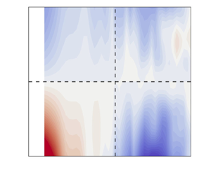
Scale-dependent inclination angle difference, $\Delta \alpha$, averaged over phase speeds (a) $\tilde {c}<0$ and (b) $\tilde {c}>0$, for different wall-normal locations. The black dashed line represents the scale of $k_x\delta = 0.5( y/\delta )^{-1}$ that appears to divide the shear-driven region in the lower-left corner from the eddy-structure region in the upper right.

For the case of slower than average phase speeds, shown in figure 9(a), we find clear evidence for a shear-dominated region near the wall, at lower wavenumbers, where the inclination angle variation, $\Delta \alpha$, is opposite (red) in sign to the phase-speed variation, $\tilde {c}$. This shear region appears to be confined by $k_x \lesssim y^{-1}$. Outside of the region, the sign between $\Delta \alpha$ and $\tilde {c}$ is reversed (blue), where we speculate that the inclination angle change is largely determined by the eddy vortex structure and not the shear. For the case of faster than average phase speeds, shown in figure 9(b), the same trends appear, although the evidence for the $k_x \lesssim y^{-1}$ cutoff is weaker. These distinct regions also appear across other Reynolds numbers, as illustrated in Appendix D. This general trend is also shown in figure 7, for large-scale, near-wall structures (right) compared with small-scale, outer structures (left).

To further support the above claim that eddy geometry and mean shear are key factors in explaining the inclination angle/phase-speed trends, we develop a crude kinematical model based on an asymmetric rigid ‘eddy’ in Appendix E. The model illustrates how the shear-driven inclination effect and the vortex structure inclination effect can result in opposite behaviour with respect to small changes in the convection velocity of an eddy. More detailed examination of the fine structure of instantaneous eddies is still needed to provide additional validation for these observations. But the basic variation of inclination angle across structures with different phase speeds appears to be the result of competing physical mechanisms in the turbulent boundary layer.