





1. Introduction
Quantitative characterization of the subsurface flow and transport processes is fundamental to predict the hydrodynamic transport of solute or heat in numerous applications, such as underground carbon storage (Hyman et al. Reference Hyman, Dentz, Hagberg and Kang2019; Wang et al. Reference Wang, Li, Liu, Xu, Liu and Wang2023), deep geothermal energy production (Yoo et al. Reference Yoo, Park, Xie, Kim, Min, Rutqvist and Rinaldi2021), underground nuclear waste disposal (Poinssot Reference Poinssot2012; Hadgu et al. Reference Hadgu, Karra, Kalinina, Makedonska, Hyman, Klise, Viswanathan and Wang2017; Tran et al. Reference Tran, Zavrin, Kersting, Klein-BenDavid, Teutsch and Weisbrod2021) and groundwater management and remediation (Neuman Reference Neuman2005).
Geological media, porous or fractured, are characterized by structural heterogeneity of hydraulic parameters at different scales. The hydraulic conductivity $ K$
of such formations can vary spatially abruptly and by several orders of magnitude: for clay or granite,
$ K$
of such formations can vary spatially abruptly and by several orders of magnitude: for clay or granite, $K$
is of the order of
$K$
is of the order of $10^{-12}\,\textrm{m s}^{-1}$
, and can reach
$10^{-12}\,\textrm{m s}^{-1}$
, and can reach $1\,\textrm{m s}^{-1}$
for coarse sand or gravel (Bear Reference Bear1972; Sanchez-Vila et al. Reference Sanchez-Vila, Guadagnini and Carrera2006). In fractured formations, the genesis of fractures is attributable to tectonic activities, exhumation-induced temperature changes or artificially induced reservoir stimulation (Gale et al. Reference Gale, Laubach, Olson, Eichhubl and Fall2014). Fractures tend to develop into networks, whose permeability is orders of magnitude higher than that of the host rock matrix. Therefore, the flow occurs predominantly through such networks of interconnected fractures, and is governed by both the transmissivity of individual fractures and the network’s connectivity and geometrical properties (Long & Witherspoon Reference Long and Witherspoon1985; Bour & Davy Reference Bour and Davy1998; de Dreuzy et al. 2002, Reference de Dreuzy, Méheust and Pichot2012; Viswanathan et al. Reference Viswanathan2022). The former strongly depends on the pore scale heterogeneity of the rough walls that constitute each fracture, while the latter determines network-scale flow patterns and the bulk volume of fluid conducted through pathways in the rock mass (Bour & Davy Reference Bour and Davy1998; Jing & Stephansson Reference Jing and Stephansson2007).
$1\,\textrm{m s}^{-1}$
for coarse sand or gravel (Bear Reference Bear1972; Sanchez-Vila et al. Reference Sanchez-Vila, Guadagnini and Carrera2006). In fractured formations, the genesis of fractures is attributable to tectonic activities, exhumation-induced temperature changes or artificially induced reservoir stimulation (Gale et al. Reference Gale, Laubach, Olson, Eichhubl and Fall2014). Fractures tend to develop into networks, whose permeability is orders of magnitude higher than that of the host rock matrix. Therefore, the flow occurs predominantly through such networks of interconnected fractures, and is governed by both the transmissivity of individual fractures and the network’s connectivity and geometrical properties (Long & Witherspoon Reference Long and Witherspoon1985; Bour & Davy Reference Bour and Davy1998; de Dreuzy et al. 2002, Reference de Dreuzy, Méheust and Pichot2012; Viswanathan et al. Reference Viswanathan2022). The former strongly depends on the pore scale heterogeneity of the rough walls that constitute each fracture, while the latter determines network-scale flow patterns and the bulk volume of fluid conducted through pathways in the rock mass (Bour & Davy Reference Bour and Davy1998; Jing & Stephansson Reference Jing and Stephansson2007).
At the scale of a single fracture, flow takes place in the void space existing between the two rough walls. Since they were originally formed by fracturing of a rock mass, the fracture walls are self-affine (Schmittbuhl et al. Reference Schmittbuhl, Schmitt and Scholz1995; Bouchaud Reference Bouchaud1997), that is, they exhibit peculiar scale invariance and spatial correlation properties. The two walls are geometrically matched, but only up to a characteristic correlation length, which implies that the aperture field is self-affine only below that scale (Brown Reference Brown1995). The aperture field is thus characterized by strong heterogeneity, with areas with wide apertures and low flow resistance contrasting with zones with low apertures, or contact zones that hinder the flow, associated with large viscous energy losses. The flow through geological fractures has been studied for nearly 40 years, using flow models either based on the depth-averaging over local apertures (Brown Reference Brown1987; Méheust & Schmittbuhl Reference Méheust and Schmittbuhl2001) or on full three-dimensional (Navier-)Stokes flow resolution (Brush & Thomson Reference Brush and Thomson2003). They have shown that aperture field heterogeneity results in flow channelling (Brown Reference Brown1987; Méheust & Schmittbuhl Reference Méheust and Schmittbuhl2001), that is, the existence of preferential flow paths up to the scale of the correlation length (Méheust & Schmittbuhl Reference Méheust and Schmittbuhl2003), which strongly impacts the fracture’s permeability. This flow heterogeneity is all the larger as the relative fracture closure $\sigma _a / \langle a\rangle$
, defined as the ratio of the aperture field’s standard deviation to its mean value, is larger. Flow heterogeneity is even more pronounced for shear-thinning fluids, which exhibit stronger flow localization than Newtonian fluids (Lenci et al. Reference Lenci, Méheust, Putti and Di Federico2022a
,
Reference Lenci, Putti, Di Federico and Méheustb
). Besides, due to the intrinsically stochastic nature of fracture geometries, and the dominant impact on the flow of the largest Fourier modes of the aperture field (Méheust & Schmittbuhl Reference Méheust and Schmittbuhl2001), a population of fractures with identical statistical geometrical parameters exhibits a very large dispersion over the hydraulic behaviour, and this all the more as the correlation length is large (Méheust & Schmittbuhl Reference Méheust and Schmittbuhl2003), so that any generic behaviour can only be obtained through a stochastic approach, considering a large number of fracture realizations (Lenci et al. Reference Lenci, Méheust, Putti and Di Federico2022a
, Reference Lenci, Méheust, Di Federico and Ciriello2024). In turn, this stochastic flow heterogeneity strongly impacts solute transport through geological fractures.
$\sigma _a / \langle a\rangle$
, defined as the ratio of the aperture field’s standard deviation to its mean value, is larger. Flow heterogeneity is even more pronounced for shear-thinning fluids, which exhibit stronger flow localization than Newtonian fluids (Lenci et al. Reference Lenci, Méheust, Putti and Di Federico2022a
,
Reference Lenci, Putti, Di Federico and Méheustb
). Besides, due to the intrinsically stochastic nature of fracture geometries, and the dominant impact on the flow of the largest Fourier modes of the aperture field (Méheust & Schmittbuhl Reference Méheust and Schmittbuhl2001), a population of fractures with identical statistical geometrical parameters exhibits a very large dispersion over the hydraulic behaviour, and this all the more as the correlation length is large (Méheust & Schmittbuhl Reference Méheust and Schmittbuhl2003), so that any generic behaviour can only be obtained through a stochastic approach, considering a large number of fracture realizations (Lenci et al. Reference Lenci, Méheust, Putti and Di Federico2022a
, Reference Lenci, Méheust, Di Federico and Ciriello2024). In turn, this stochastic flow heterogeneity strongly impacts solute transport through geological fractures.
Starting from the pioneering works of De Josselin De Jong (Reference De Josselin De Jong1958) and Saffman (Reference Saffman1959), significant efforts have been dedicated to systematically quantifying solute or heat transport in heterogeneous porous and fractured media through stochastic modelling (Dagan Reference Dagan1989; Gelhar Reference Gelhar1993; Rubin Reference Rubin2003; Yeh et al. Reference Yeh, Khaleel and Carroll2015). In particular, the onset of anomalous (i.e. non-Fickian) dispersion has been a subject of debate: laboratory and in situ observations showed its dependence on a reference scale (Gelhar et al. Reference Gelhar, Welty and Rehfeldt1992), indicating that it arises as a direct result of medium heterogeneity (Warren & Skiba Reference Warren and Skiba1964; Pickens & Grisak Reference Pickens and Grisak1981; Silliman & Simpson Reference Silliman and Simpson1987). A unified theory explaining scale effects in both flow and transport based on the underlying fractal structure of the hydraulic conductivity field of a porous medium was proposed by Di Federico & Neuman (Reference Di Federico and Neuman1997, Reference Di Federico and Neuman1998a , Reference Di Federico and Neumanb ). In low-heterogeneity porous media characterized by a single and finite integral scale, the macrodispersion coefficient evolves in time in the preasymptotic regime and tends to a constant asymptotic Fickian value proportional to the variance of the logarithm of hydraulic conductivity (Dagan Reference Dagan1984). Recent research has established that anomalous transport phenomena in fractured media are deeply connected to structural heterogeneities such as mean aperture variability and correlation length, and that these can be effectively captured through stochastic frameworks such as continuous time random walk (CTRW) models. For instance, Hyman et al. (Reference Hyman, Dentz, Hagberg and Kang2019) and Hyman & Dentz (Reference Hyman and Dentz2021) investigated how flow channelling and network-scale structure in three-dimensional discrete fracture networks control Lagrangian velocity distributions and transport signatures, linking transport behaviours to the underlying network topology. Edery et al. (Reference Edery, Geiger and Berkowitz2016) emphasized the role of fracture aperture orientation and heterogeneity within the network in shaping breakthrough curve (BTC) tailing. Sund et al. (Reference Sund, Parashar and Pham2021) and Elhanati et al. (Reference Elhanati, Goeppert and Berkowitz2024) extended these analyses to karst and fractured aquifers, showing how large-scale structural features and temporal rainfall variability drive transport anomalies.
For single fractures, early studies of solute transport have addressed the purely self-affine aperture field (Roux et al. Reference Roux, Plouraboué and Hulin1996; Plouraboué et al. Reference Plouraboué, Hulin, Roux and Koplik1998; Drazer et al. Reference Drazer, Auradou, Koplik and Hulin2004), focusing on the link between the geometry of the solute front and that of the fracture. More recently, mostly numerical studies (Thompson Reference Thompson1991; Wang & Cardenas Reference Wang and Cardenas2014) have addressed solute transport in single fracture geometries. Wang & Cardenas (Reference Wang and Cardenas2014) successfully adopted a CTRW approach to reproduce non-Fickian transport behaviours from experiments by Cardenas et al. (Reference Cardenas, Slottke, Ketcham and Sharp2007), such as early solute breakthrough and heavy tailing in BTCs. They found that predictions from the standard advection–dispersion equation became increasingly inaccurate when closing the fracture, while the CTRW model provided significantly better fits to the BTCs.
Stochastic transport in fractures has also been addressed in studies based on heterogeneous transmissivity fields, including those of Cvetkovic & Gotovac (Reference Cvetkovic and Gotovac2014) and Fiori & Becker (Reference Fiori and Becker2015). In these works, transmissivity heterogeneity was modelled through multi-Gaussian random fields with prescribed variance and spatial correlation structure. These and other works on transport in highly heterogeneous multi-Gaussian conductivity fields (most of them addressing porous media rather than fractures) (Fiori et al. Reference Fiori, Janković, Dagan and Cvetković2007; Le Borgne et al. Reference Le Borgne, Dentz and Carrera2008; Gotovac et al. Reference Gotovac, Cvetkovic and Andricevic2009; Comolli et al. Reference Comolli, Hakoun and Dentz2019) have identified non-Fickian transport signatures characterized by early breakthrough and power-law BTC tailing. These transport signatures have also been upscaled using stochastic modelling approaches based on time-domain and CTRWs (Delay et al. Reference Delay, Porel and Sardini2002; Berkowitz et al. Reference Berkowitz, Cortis, Dentz and Scher2006; Cvetkovic et al. Reference Cvetkovic, Fiori and Dagan2014; Noetinger et al. Reference Noetinger, Roubinet, Russian, Le Borgne, Delay, Dentz, de Dreuzy and Gouze2016).
Given the experimentally documented self-affine nature of natural fracture walls (Schmittbuhl et al. Reference Schmittbuhl, Schmitt and Scholz1995; Bouchaud Reference Bouchaud1997), an alternative and physically grounded description consists in deriving transmissivity variability directly from the fracture geometry. In this framework, velocity statistics emerge from aperture fluctuations through the Reynolds equation governing flow in rough fractures. The present study adopts this approach to investigate how the fracture’s two main geometric parameters, the relative closure $\sigma _a/\langle a \rangle$
and the correlation length
$\sigma _a/\langle a \rangle$
and the correlation length $L_{\textit{c}}$
, control the velocity distributions and the associated purely advective (i.e. infinite Péclet) transport behaviour, under Stokes (i.e. creeping) flow conditions. We perform a stochastic analysis to account for the potential strong variability among the solute transport behaviour of fracture realizations with identical geometrical parameters. We investigate preasymptotic non-Fickian transport, and discuss the approach of the asymptotic Fickian behaviour. We also investigate the impact of initial conditions (i.e. flux-weighted or uniform injection). To the best of our knowledge, this is the first study that investigates the impact of the mean fracture aperture (or, equivalently, mean transmissivity) on advective transport considering a transmissivity field that relies both on self-affinity of the aperture field below the correlation length and on a Gaussian probability density function (PDF) of the local apertures. It is also the first study of transport in geological fractures that adopts a stochastic approach in which many fractures described by the same statistical geometrical parameters are considered, with results being interpreted in terms of both the mean behaviour of the population and the fluctuations of the statistics around that mean. Because flow channelling in a rough fracture is sensitive to the particular realization of the aperture field, considering a single fracture does not, in general, provide a behaviour that is representative of the mean behaviour of the population. This is particularly true when the correlation length is not much smaller than the fracture size, so that the sampled aperture structures are not representative of the ensemble. Here, we show how fluctuations around the ensemble average decrease when the correlation length becomes very small with respect to the fracture size; this is the limit for which ergodicity can be considered to hold for any given fracture of the population. Hence, we do not postulate ergodic representativeness a priori for advective transport, but show how it appears in the limit of very small correlation lengths.
$L_{\textit{c}}$
, control the velocity distributions and the associated purely advective (i.e. infinite Péclet) transport behaviour, under Stokes (i.e. creeping) flow conditions. We perform a stochastic analysis to account for the potential strong variability among the solute transport behaviour of fracture realizations with identical geometrical parameters. We investigate preasymptotic non-Fickian transport, and discuss the approach of the asymptotic Fickian behaviour. We also investigate the impact of initial conditions (i.e. flux-weighted or uniform injection). To the best of our knowledge, this is the first study that investigates the impact of the mean fracture aperture (or, equivalently, mean transmissivity) on advective transport considering a transmissivity field that relies both on self-affinity of the aperture field below the correlation length and on a Gaussian probability density function (PDF) of the local apertures. It is also the first study of transport in geological fractures that adopts a stochastic approach in which many fractures described by the same statistical geometrical parameters are considered, with results being interpreted in terms of both the mean behaviour of the population and the fluctuations of the statistics around that mean. Because flow channelling in a rough fracture is sensitive to the particular realization of the aperture field, considering a single fracture does not, in general, provide a behaviour that is representative of the mean behaviour of the population. This is particularly true when the correlation length is not much smaller than the fracture size, so that the sampled aperture structures are not representative of the ensemble. Here, we show how fluctuations around the ensemble average decrease when the correlation length becomes very small with respect to the fracture size; this is the limit for which ergodicity can be considered to hold for any given fracture of the population. Hence, we do not postulate ergodic representativeness a priori for advective transport, but show how it appears in the limit of very small correlation lengths.
To model transport numerically, we employ two complementary approaches: a time-domain random walk (TDRW) that directly tracks fluid particles, and an upscaled one-dimensional spatial CTRW framework in which the fluctuating Lagrangian velocity series is represented by an Ornstein–Uhlenbeck process (Dentz et al. Reference Dentz, Kang, Comolli, Le Borgne and Lester2016; Kang et al. Reference Kang, Dentz, Le Borgne, Lee and Juanes2017; Morales et al. Reference Morales, Dentz, Willmann and Holzner2017). Such random walk approaches, which directly model particle motion in heterogeneous media, have been proposed to investigate non-Fickian behaviour while avoiding numerical diffusion. Among random walks, TDRWs have been adopted to model particle motion, relying on evenly displacing particles along streamlines with variable residence times (Noetinger et al. Reference Noetinger, Roubinet, Russian, Le Borgne, Delay, Dentz, de Dreuzy and Gouze2016), as the flow field is organized on fixed length scales (Berkowitz & Scher Reference Berkowitz and Scher1997; Benke & Painter Reference Benke and Painter2003; Kang et al. Reference Kang, Dentz, Le Borgne and Juanes2011). The TDRWs are computationally efficient as they avoid unnecessary iterations in low-velocity zones. The CTRW upscaling formulations, on the other hand, allow linking transport scaling to the low-velocity structure of the flow field (Painter et al. Reference Painter, Cvetkovic and Selroos2002; Comolli et al. Reference Comolli, Hakoun and Dentz2019; Puyguiraud et al. Reference Puyguiraud, Gouze and Dentz2019; Hyman & Dentz Reference Hyman and Dentz2021; Dentz & Hyman Reference Dentz and Hyman2023). The simulations show that, in single synthetic fractures with realistic wall roughness, the interplay of relative closure and correlation length gives rise to a wide range of transport regimes, even in the high-Péclet limit. Moreover, these behaviours can be efficiently captured using the upscaled CTRW-based Ornstein–Uhlenbeck model, validating its application at the fracture scale and confirming its robustness to link fracture geometry to macroscopic transport scaling, under moderate ergodicity conditions, from the sole knowledge of the velocity statistics, flow tortuosity and a Lagrangian correlation length. In addition, the CTRW model allows us to theoretically predict the exponents of long time power law exponents in the BTCs from the low velocity asymptotic behaviour of the Eulerian velocities’ PDF.
The organization of the article is as follows: § 2.1 describes rough fracture geometries and how synthetic fractures with such geometries can be generated numerically, the derivation of the Reynolds equation describing depth-averaged Stokes flow, and the finite-volume Stokes-flow solver. Section 2.2 presents the models of hydrodynamic transport in heterogeneous media, which are a time domain random walk particle tracking scheme and a one-dimensional upscaled model based on a CTRW. Section 3 reports on the results of the stochastic analysis for the velocity field and advective transport. Section 4 summarizes the study and provides potential further prospects for future studies.
2. Methods
We investigate advective transport through synthetic rough-walled geological fractures. The modelling framework presented here relies on the following assumptions. The flow is assumed to be steady, incompressible and isothermal, and is governed by the Stokes equations. Because of the small fracture aperture and the gradual spatial variation of the walls, we adopt the lubrication approximation, yielding the two-dimensional Reynolds equation. Fracture walls are modelled as self-affine and statistically isotropic, with their mutual matching controlled by a finite correlation length. Ideal plastic closure is used to model contact zones, i.e. negative aperture values are set to zero. Particle transport is modelled in the purely advective limit (i.e. at infinite Péclet number). The transported entities are fluid particles, which have no mass, follow streamlines and interact neither with the solid boundaries nor with each other.
2.1. Flow in geological fractures
2.1.1. Heterogeneous aperture fields
The aperture field $a$
of a geological fracture is defined as the distance between the two wall topographies along the direction perpendicular to the fracture’s mean plane. For a fracture whose mean plane is horizontal, if the top and bottom wall topographies (each with zero mean) are denoted, respectively, by
$a$
of a geological fracture is defined as the distance between the two wall topographies along the direction perpendicular to the fracture’s mean plane. For a fracture whose mean plane is horizontal, if the top and bottom wall topographies (each with zero mean) are denoted, respectively, by $h_{\textit{u}}$
and
$h_{\textit{u}}$
and $h_{\textit{b}}$
, then the aperture field is
$h_{\textit{b}}$
, then the aperture field is
 \begin{equation} a({\boldsymbol{x}}) = h_{\textit{u}}({\boldsymbol{x}})\;-\;h_{\textit{b}}({\boldsymbol{x}})\;+\;a_{\textit{m}}, \end{equation}
where the mechanical aperture $a_{\text{m}}$
is the distance between the mean planes of the wall topographies, and
$a_{\text{m}}$
is the distance between the mean planes of the wall topographies, and ${\boldsymbol{x}} = (x_1,x_2)^\top$
is the position vector in the
${\boldsymbol{x}} = (x_1,x_2)^\top$
is the position vector in the $(x_1,x_2)$
plane (with
$(x_1,x_2)$
plane (with $\top$
denoting the transpose).
$\top$
denoting the transpose).
The fracturing process that forms the fracture causes the fracture walls’ topography to exhibit self-affine scale invariance across all scales (Bouchaud et al. Reference Bouchaud, Lapasset and Planès1990; Schmittbuhl et al. Reference Schmittbuhl, Schmitt and Scholz1995; Candela et al. Reference Candela, Renard, Bouchon, Brouste, Marsan, Schmittbuhl and Voisin2009). One consequence of this self-affinity is that the two-dimensional power spectral density $\mathcal{G}$
of the wall topography scales as a power law of the wavenumber modulus
$\mathcal{G}$
of the wall topography scales as a power law of the wavenumber modulus $k$
, namely
$k$
, namely
 \begin{equation} \mathcal{G}\propto k^{-2(H + 1)}, \end{equation}
where $H$
is the so-called Hurst exponent (Schmittbuhl et al. Reference Schmittbuhl, Schmitt and Scholz1995). The value of
$H$
is the so-called Hurst exponent (Schmittbuhl et al. Reference Schmittbuhl, Schmitt and Scholz1995). The value of $H$
, governed by the fracturing process, typically lies in the range
$H$
, governed by the fracturing process, typically lies in the range $[0.5, 0.9]$
and is nearly universal (close to 0.8) for most brittle materials, including igneous rocks such as granite and basalt (Bouchaud et al. Reference Bouchaud, Lapasset and Planès1990; Méheust & Schmittbuhl Reference Méheust and Schmittbuhl2000). A value of 0.5 is usually measured in sandstone, due to its intergranular fracturing (Boffa et al. Reference Boffa, Allain, Chertcoff, Hulin, Plouraboué and Roux1999). In any case, the Hurst exponent can be considered a petrophysical parameter of the geological formation.
$[0.5, 0.9]$
and is nearly universal (close to 0.8) for most brittle materials, including igneous rocks such as granite and basalt (Bouchaud et al. Reference Bouchaud, Lapasset and Planès1990; Méheust & Schmittbuhl Reference Méheust and Schmittbuhl2000). A value of 0.5 is usually measured in sandstone, due to its intergranular fracturing (Boffa et al. Reference Boffa, Allain, Chertcoff, Hulin, Plouraboué and Roux1999). In any case, the Hurst exponent can be considered a petrophysical parameter of the geological formation.
The walls of a fresh brittle fracture are identical at all scales. In contrast, in geological fractures, due to the combined action (over geological times) of chemical weathering and interaction between the fracture walls, such as tectonics-induced relative movement and mechanical grinding, their topographies are only matched at scales larger than a characteristic matching scale that we denote the correlation length $L_{\textit{c}}$
(Brown Reference Brown1995). Consequently, the aperture field, being related to the two topographies through (2.1), retains self-affine scaling only at scales smaller than
$L_{\textit{c}}$
(Brown Reference Brown1995). Consequently, the aperture field, being related to the two topographies through (2.1), retains self-affine scaling only at scales smaller than $L_{\textit{c}}$
. In particular, the power spectral density of the aperture field only exhibits a power law of the type presented in (2.2) at wavenumbers larger than
$L_{\textit{c}}$
. In particular, the power spectral density of the aperture field only exhibits a power law of the type presented in (2.2) at wavenumbers larger than $k_{\textit{c}} = 2\pi / L_{\textit{c}}$
.
$k_{\textit{c}} = 2\pi / L_{\textit{c}}$
.
In this work, fracture aperture fields are thus generated according to the algorithm proposed by Méheust & Schmittbuhl (Reference Méheust and Schmittbuhl2001) and Lenci et al. (Reference Lenci, Putti, Di Federico and Méheust2022b
). Specifically, the algorithm enforces (2.2) for wavenumbers $k \gt k_{\textit{c}}$
, corresponding to scales smaller than the correlation length, and assumes no dependence on
$k \gt k_{\textit{c}}$
, corresponding to scales smaller than the correlation length, and assumes no dependence on $k$
for
$k$
for $k \leqslant k_{\textit{c}}$
. This ensures that the aperture field is self-affine up to the correlation length
$k \leqslant k_{\textit{c}}$
. This ensures that the aperture field is self-affine up to the correlation length $L_{\textit{c}}$
and uncorrelated beyond it. This is achieved by multiplying the two-dimensional white-noise Fourier transform by
$L_{\textit{c}}$
and uncorrelated beyond it. This is achieved by multiplying the two-dimensional white-noise Fourier transform by
 \begin{equation} \biggl [\max \Bigl (\sqrt {k_{x_1}^2 + k_{x_2}^2},\,k_{\textit{c}}\Bigr )\biggr ]^{-2(H+1)}, \end{equation}
and then taking the inverse Fourier transform of the product to generate a two-dimensional isotropic aperture field. Finally, the aperture field is rescaled and translated to match the desired mean, $\langle a\rangle$
, and standard deviation,
$\langle a\rangle$
, and standard deviation, $\sigma _a$
. If the relative fracture closure, defined as
$\sigma _a$
. If the relative fracture closure, defined as $\sigma _a / \langle a\rangle$
, is sufficiently large, some regions of the generated aperture field may become negative; these are set to zero (ideal plastic closure). In such cases, the mean aperture
$\sigma _a / \langle a\rangle$
, is sufficiently large, some regions of the generated aperture field may become negative; these are set to zero (ideal plastic closure). In such cases, the mean aperture $\langle a\rangle$
no longer coincides with the mechanical aperture
$\langle a\rangle$
no longer coincides with the mechanical aperture $a_{\textit{m}}$
. Throughout § 3, we therefore characterize fracture closure using
$a_{\textit{m}}$
. Throughout § 3, we therefore characterize fracture closure using $\sigma _a / \langle a \rangle$
. Figure 1 provides an illustration of fracture geometries and their corresponding spectral characteristics. Figure 1(a) presents one longitudinal profile of a synthetic rough fracture, where the fracture walls are depicted along with the key geometric fields that define the fracture geometry. In figure 1(b), the power spectrum is shown for two different values of
$\sigma _a / \langle a \rangle$
. Figure 1 provides an illustration of fracture geometries and their corresponding spectral characteristics. Figure 1(a) presents one longitudinal profile of a synthetic rough fracture, where the fracture walls are depicted along with the key geometric fields that define the fracture geometry. In figure 1(b), the power spectrum is shown for two different values of $L/L_{\textit{c}}$
, showing the cutoff of the power law behaviour at
$L/L_{\textit{c}}$
, showing the cutoff of the power law behaviour at $k_{\textit{c}}$
. Figure 1(c) shows aperture fields and corresponding PDFs for closures of 0.25 and 0.75, each at two system sizes:
$k_{\textit{c}}$
. Figure 1(c) shows aperture fields and corresponding PDFs for closures of 0.25 and 0.75, each at two system sizes: $L/L_{\textit{c}} = 2^3$
and
$L/L_{\textit{c}} = 2^3$
and $L/L_{\textit{c}} = 2^5$
. The generated aperture fields are self-affine up to
$L/L_{\textit{c}} = 2^5$
. The generated aperture fields are self-affine up to $L_{\textit{c}}$
, i.e. they exhibit long-range correlations up to that scale. This explains why the largest areas of approximately uniform colour have a characteristic size of order
$L_{\textit{c}}$
, i.e. they exhibit long-range correlations up to that scale. This explains why the largest areas of approximately uniform colour have a characteristic size of order $L_{\textit{c}}$
; the size of the closed regions also reflects the value of
$L_{\textit{c}}$
; the size of the closed regions also reflects the value of $L_{\textit{c}}$
, for the same reason. Note that in the limit
$L_{\textit{c}}$
, for the same reason. Note that in the limit $L/L_{\textit{c}} \to 1$
, the aperture field would approach uniformity. Additionally, the numerical discretization introduces an implicit small-scale cutoff at the grid size. The unresolved finescale roughness is, in reality, a continuation of the self-affine behaviour down to micrometric length scales. Since small-scale spectral modes have diminishing influence on the flow organization, resolving the geometry more would not result in a significantly different velocity field. The adopted spatial resolution (
$L/L_{\textit{c}} \to 1$
, the aperture field would approach uniformity. Additionally, the numerical discretization introduces an implicit small-scale cutoff at the grid size. The unresolved finescale roughness is, in reality, a continuation of the self-affine behaviour down to micrometric length scales. Since small-scale spectral modes have diminishing influence on the flow organization, resolving the geometry more would not result in a significantly different velocity field. The adopted spatial resolution ( $2^{10}$
control volumes per side) ensures that geometric features are accurately represented down to the grid scale, which is much smaller than the correlation length in all cases. Finally, the PDF of the local apertures is approximately Gaussian in all cases, as shown in figure 1(c), with a cutoff at zero when contact regions are present in the fracture plane.
$2^{10}$
control volumes per side) ensures that geometric features are accurately represented down to the grid scale, which is much smaller than the correlation length in all cases. Finally, the PDF of the local apertures is approximately Gaussian in all cases, as shown in figure 1(c), with a cutoff at zero when contact regions are present in the fracture plane.
Overview of the geometries and associated spectra from synthetic geological fractures. Panel (a) shows one longitudinal profile of the fracture, with the representation of the walls and the definition of the geometrical fields that define the fracture geometry. Panel (b) presents the power spectrum for the cases $L/L_{\textit{c}} = 2^5$
in red and
$L/L_{\textit{c}} = 2^5$
in red and $L/L_{\textit{c}} = 2^3$
in green. Panel (c) shows four aperture field realizations arranged from (i) to (iv), each with its corresponding local aperture PDF displayed below. Realizations (i) and (ii) correspond to
$L/L_{\textit{c}} = 2^3$
in green. Panel (c) shows four aperture field realizations arranged from (i) to (iv), each with its corresponding local aperture PDF displayed below. Realizations (i) and (ii) correspond to $L/L_{\textit{c}} = 2^3$
with closure values of 0.25 and 0.75, respectively, while (iii) and (iv) correspond to
$L/L_{\textit{c}} = 2^3$
with closure values of 0.25 and 0.75, respectively, while (iii) and (iv) correspond to $L/L_{\textit{c}} = 2^5$
, also with closures of 0.25 and 0.75. In all cases, the local aperture PDFs are approximately Gaussian, with a cutoff at zero when contact regions are present in the fracture plane.
$L/L_{\textit{c}} = 2^5$
, also with closures of 0.25 and 0.75. In all cases, the local aperture PDFs are approximately Gaussian, with a cutoff at zero when contact regions are present in the fracture plane.

Figure 1. Long description
Panel A: A line graph displays one longitudinal profile of a fracture, with the representation of the walls and the definition of the geometrical fields that define the fracture geometry. The x-axis is labeled x1/L and the y-axis is labeled h/a_m. The graph shows two sections, one above and one below the horizontal axis, with annotations indicating (h_u/a_m) + 0.5 and (h_b/a_m) - 0.5. Panel B: A line graph presents the power spectrum for two cases, one in red and one in green. The x-axis is labeled Log2 k and the y-axis is labeled Log2 G(k). The graph shows two lines representing different ratios of L/L_c, with annotations indicating L/L_c = 2^3 and L/L_c = 2^5. Panel C: Four images show aperture field realizations arranged from (i) to (iv), each with its corresponding local aperture PDF displayed below. The x-axis of the PDF graphs is labeled a/<a> and the y-axis is labeled PDF. The images and graphs illustrate different closure values and the associated probability density functions.
Geological fractures typically have mean apertures ranging from tens of microns to several millimetres. In this work, we set $\langle a\rangle = 1$
mm, representative of typical fracture apertures in crystalline and sedimentary rocks, as indicated by various laboratory measurements (Watanabe et al. Reference Watanabe, Hirano and Tsuchiya2008). Furthermore, we consider two different values of the fracture relative closure
$\langle a\rangle = 1$
mm, representative of typical fracture apertures in crystalline and sedimentary rocks, as indicated by various laboratory measurements (Watanabe et al. Reference Watanabe, Hirano and Tsuchiya2008). Furthermore, we consider two different values of the fracture relative closure $\sigma _a/\langle a\rangle$
to represent distinct degrees of aperture variability. We also fix the correlation length to
$\sigma _a/\langle a\rangle$
to represent distinct degrees of aperture variability. We also fix the correlation length to $L_{\textit{c}} = 0.1\,\mathrm{m}$
, based on characteristic lengths observed in fractured rock outcrops and laboratory studies (Brown Reference Brown1995; Méheust & Schmittbuhl Reference Méheust and Schmittbuhl2000). We then vary the fracture length
$L_{\textit{c}} = 0.1\,\mathrm{m}$
, based on characteristic lengths observed in fractured rock outcrops and laboratory studies (Brown Reference Brown1995; Méheust & Schmittbuhl Reference Méheust and Schmittbuhl2000). We then vary the fracture length $L$
, so as to obtain different values of the ratio
$L$
, so as to obtain different values of the ratio $L/L_{\textit{c}}$
. This means that we consider the correlation length to be a property of the fracturing process, which is uniform over a given fractured medium; fractures of different lengths within that medium still exhibit the same correlation length
$L/L_{\textit{c}}$
. This means that we consider the correlation length to be a property of the fracturing process, which is uniform over a given fractured medium; fractures of different lengths within that medium still exhibit the same correlation length $L_{\textit{c}}$
.
$L_{\textit{c}}$
.
2.1.2. Flow equation
Under steady and isothermal conditions, the viscous flow of an incompressible fluid through a fracture of variable aperture $a=a(x_1,x_2)$
is governed by the Stokes equations
$a=a(x_1,x_2)$
is governed by the Stokes equations
 \begin{align} \boldsymbol{\nabla }' P &= \mu \boldsymbol{\nabla} ^{\prime 2}\boldsymbol{u}', \quad \boldsymbol{\nabla }'\boldsymbol{\cdot }\boldsymbol{u}' = 0, \end{align}
where $\boldsymbol{x}=(x_1,x_2,x_3)^\top$
is the position vector,
$\boldsymbol{x}=(x_1,x_2,x_3)^\top$
is the position vector, $\mu$
is the fluid’s dynamic viscosity,
$\mu$
is the fluid’s dynamic viscosity, $\boldsymbol{u}'=(u_1,u_2,u_3)^{\top }$
is the velocity field,
$\boldsymbol{u}'=(u_1,u_2,u_3)^{\top }$
is the velocity field, $P$
is the pressure field (including gravity effects) and
$P$
is the pressure field (including gravity effects) and $\boldsymbol{\nabla }'$
is the gradient operator. If the aperture field
$\boldsymbol{\nabla }'$
is the gradient operator. If the aperture field $a$
is sufficiently smooth, we apply the lubrication approximation, according to which the in-plane component of the velocity field is much larger than its out-of-plane component. It follows that the gap-averaged velocity field,
$a$
is sufficiently smooth, we apply the lubrication approximation, according to which the in-plane component of the velocity field is much larger than its out-of-plane component. It follows that the gap-averaged velocity field, $\boldsymbol{u}= (u_1,u_2)^{\top }$
, satisfies the Darcy-type equation (Zimmerman & Bodvarsson Reference Zimmerman and Bodvarsson1996)
$\boldsymbol{u}= (u_1,u_2)^{\top }$
, satisfies the Darcy-type equation (Zimmerman & Bodvarsson Reference Zimmerman and Bodvarsson1996)
 \begin{align} {\boldsymbol{u}} = - \frac {a^2}{12 \mu } \boldsymbol{\nabla }\!P, \end{align}
at any position within the mean fracture plane and with $ \boldsymbol{\nabla}$
denoting the gradient operator in the
$ \boldsymbol{\nabla}$
denoting the gradient operator in the $(x_1,x_2)$
plane. Since the three-dimensional velocity field
$(x_1,x_2)$
plane. Since the three-dimensional velocity field $\boldsymbol{u}^\prime$
is divergence-free, the depth-integrated velocity
$\boldsymbol{u}^\prime$
is divergence-free, the depth-integrated velocity $\boldsymbol{q} = a\,\boldsymbol{u}$
, previously referred to as the local flux (Méheust & Schmittbuhl Reference Méheust and Schmittbuhl2001), also satisfies the continuity condition
$\boldsymbol{q} = a\,\boldsymbol{u}$
, previously referred to as the local flux (Méheust & Schmittbuhl Reference Méheust and Schmittbuhl2001), also satisfies the continuity condition $\boldsymbol{\nabla }\!\boldsymbol{\cdot }\!\boldsymbol{q} = 0$
. By combining this condition and (2.5), one then obtains the Reynolds equation governing the pressure distribution within the fracture:
$\boldsymbol{\nabla }\!\boldsymbol{\cdot }\!\boldsymbol{q} = 0$
. By combining this condition and (2.5), one then obtains the Reynolds equation governing the pressure distribution within the fracture:
 \begin{equation}\boldsymbol{\nabla }\boldsymbol{\cdot }(a^3 \boldsymbol{\nabla }\!P) =0. \end{equation}
We determine the PDF of Eulerian flow velocities $u_e({\boldsymbol{x}}) = \|{\boldsymbol{u}}({\boldsymbol{x}})\|$
by spatial sampling in the flow domain
$u_e({\boldsymbol{x}}) = \|{\boldsymbol{u}}({\boldsymbol{x}})\|$
by spatial sampling in the flow domain $\varOmega$
of area
$\varOmega$
of area $|\varOmega |$
:
$|\varOmega |$
:
 \begin{align} f_e(u) = \frac {1}{|\varOmega |} \int _{\varOmega } \text{d}\boldsymbol{x}\; \delta [u - u_e(\boldsymbol{x})]. \end{align}
Furthermore, we calculate the advective tortuosity, which is given by
 \begin{align} \chi = \frac {\langle u_e \rangle }{\langle u_1\rangle }, \end{align}
where the angular brackets denote spatial averaging. The advective tortuosity $\chi$
quantifies how much the average particle trajectories deviate from the mean flow direction due to flow channelling. It measures the geometric elongation of transport paths and is critical for relating streamwise distances to longitudinal displacements in upscaled models.
$\chi$
quantifies how much the average particle trajectories deviate from the mean flow direction due to flow channelling. It measures the geometric elongation of transport paths and is critical for relating streamwise distances to longitudinal displacements in upscaled models.
(a) Representation of the domain partitioning with boundary conditions. (b) Finite volume scheme five-point stencil: pressure is defined at the centre of each control volume, while the local aperture is estimated along the edge of the cells by arithmetic averaging.

2.1.3. Numerical implementation
The fracture is modelled as a two-dimensional square domain ( $\varOmega$
) of side length
$\varOmega$
) of side length $L$
and boundary
$L$
and boundary $\partial \varOmega =\partial \varOmega _{\textit{D}}\cup \partial \varOmega _{\textit{N}}$
, as shown in figure 2(a). This domain corresponds to the projection of the fracture volume onto its mean plane, positioned at an equal distance between the mean planes of the two walls (which are parallel to each other). The flow (2.6) is solved numerically under the action of an externally imposed macroscopic pressure gradient
$\partial \varOmega =\partial \varOmega _{\textit{D}}\cup \partial \varOmega _{\textit{N}}$
, as shown in figure 2(a). This domain corresponds to the projection of the fracture volume onto its mean plane, positioned at an equal distance between the mean planes of the two walls (which are parallel to each other). The flow (2.6) is solved numerically under the action of an externally imposed macroscopic pressure gradient $\overline {\boldsymbol{\nabla }\!P}$
. Along the left- and right-hand side of the fracture (
$\overline {\boldsymbol{\nabla }\!P}$
. Along the left- and right-hand side of the fracture ( $\partial \varOmega _{\textit{D}}$
), Dirichlet boundary conditions are considered:
$\partial \varOmega _{\textit{D}}$
), Dirichlet boundary conditions are considered: $P(0,x_2)=\overline {\boldsymbol{\nabla }\!P}\, L$
and
$P(0,x_2)=\overline {\boldsymbol{\nabla }\!P}\, L$
and $P(L,x_2)=0$
, respectively. Neumann boundary conditions are imposed on the remaining portion of the boundary (
$P(L,x_2)=0$
, respectively. Neumann boundary conditions are imposed on the remaining portion of the boundary ( $\partial \varOmega _{\textit{N}}$
). The aperture field
$\partial \varOmega _{\textit{N}}$
). The aperture field $a({\boldsymbol{x}})$
is defined over a discrete regular partition of
$a({\boldsymbol{x}})$
is defined over a discrete regular partition of $\varOmega$
in
$\varOmega$
in $n^2$
non-overlapping control volumes
$n^2$
non-overlapping control volumes $\omega$
of linear size
$\omega$
of linear size $\Delta x=L/n$
, with
$\Delta x=L/n$
, with $n=2^{10}$
. This ensures that both the geometric heterogeneity and the resulting velocity gradients are well resolved; for instance, when
$n=2^{10}$
. This ensures that both the geometric heterogeneity and the resulting velocity gradients are well resolved; for instance, when $L_{\textit{c}} = 0.1$
m, and
$L_{\textit{c}} = 0.1$
m, and $L/L_{\textit{c}}=32$
, the domain size
$L/L_{\textit{c}}=32$
, the domain size $L$
is 3.2 m and that of each control volume is
$L$
is 3.2 m and that of each control volume is $\Delta x = 3.1$
mm, which is comparable to the mean aperture. Consequently, the convergence of the pressure and velocity fields is ensured, in good consistency with prior studies (Méheust & Schmittbuhl Reference Méheust and Schmittbuhl2001; Lenci et al. Reference Lenci, Putti, Di Federico and Méheust2022b
). Figure 2(a) shows a schematic of the computational domain, the partitioning into finite volumes, and the boundary conditions applied. A finite-volume discretization of the Reynolds equation is formulated to solve the equation (as shown in figure 2
b). For each control volume
$\Delta x = 3.1$
mm, which is comparable to the mean aperture. Consequently, the convergence of the pressure and velocity fields is ensured, in good consistency with prior studies (Méheust & Schmittbuhl Reference Méheust and Schmittbuhl2001; Lenci et al. Reference Lenci, Putti, Di Federico and Méheust2022b
). Figure 2(a) shows a schematic of the computational domain, the partitioning into finite volumes, and the boundary conditions applied. A finite-volume discretization of the Reynolds equation is formulated to solve the equation (as shown in figure 2
b). For each control volume $\omega _{\!j}$
, whose set of neighbouring control volumes is indexed as
$\omega _{\!j}$
, whose set of neighbouring control volumes is indexed as $\sigma (j)=\{N, S, E, W\}$
, the following linear equation holds:
$\sigma (j)=\{N, S, E, W\}$
, the following linear equation holds:
 \begin{equation} \sum \limits _{k\in \sigma (j)} c_{k}^{(j)}(p_{k}-p_{\!j})=0, \end{equation}
where $p_i$
denotes the pressure in the centre of the
$p_i$
denotes the pressure in the centre of the $i$
th cell, and the coefficient
$i$
th cell, and the coefficient $c_k^{(j)}=(a_k+a_{\!j})^3/(8 \Delta x^2)$
is obtained as the arithmetic average of the local apertures of cells
$c_k^{(j)}=(a_k+a_{\!j})^3/(8 \Delta x^2)$
is obtained as the arithmetic average of the local apertures of cells $k$
and
$k$
and $j$
. It is the same in the
$j$
. It is the same in the $1$
- and
$1$
- and $2$
-directions. Note that the harmonic mean would be energetically consistent and thus preferable in principle, but we chose to employ the arithmetic mean to mitigate numerical instability issues. Specifically, the arithmetic average is less sensitive to the ill-conditioning caused by the strong aperture variability, which can span several orders of magnitude (Mazzia et al. Reference Mazzia, Manzini and Putti2011). The coordinate of the centre point of the pixel
$2$
-directions. Note that the harmonic mean would be energetically consistent and thus preferable in principle, but we chose to employ the arithmetic mean to mitigate numerical instability issues. Specifically, the arithmetic average is less sensitive to the ill-conditioning caused by the strong aperture variability, which can span several orders of magnitude (Mazzia et al. Reference Mazzia, Manzini and Putti2011). The coordinate of the centre point of the pixel $i$
is denoted by
$i$
is denoted by ${\boldsymbol{x}}^{(i)}$
. Equation (2.9) is equivalent to the linear system
${\boldsymbol{x}}^{(i)}$
. Equation (2.9) is equivalent to the linear system $\boldsymbol{A}\! \boldsymbol{p}=\boldsymbol{f}$
, whose coefficient matrix
$\boldsymbol{A}\! \boldsymbol{p}=\boldsymbol{f}$
, whose coefficient matrix $\boldsymbol{A}$
is
$\boldsymbol{A}$
is
 \begin{equation} A_{ij}= \begin{cases} -\sum \limits _{\substack {k\in \sigma (j)}}c_{k}^{(j)} \quad &\textrm {if} \quad i=j;\\[15pt] c_{i}^{(j)}\quad &\textrm {if} \quad i\in \sigma (j);\\[7pt] 0 \quad &\textrm {otherwise,} \end{cases}\, \end{equation}
while the vector $\mathbf f$
is
$\mathbf f$
is
 \begin{equation} f_{\!j}= -c_{W}^{(j)}\overline {\boldsymbol{\nabla }\!P}\, L, \end{equation}
at the nodes in the left-hand boundary and zero otherwise. The system is well-posed provided that the coefficient matrix $\boldsymbol{A}$
is an M-matrix, which is ensured in this case by strictly positive diagonal entries
$\boldsymbol{A}$
is an M-matrix, which is ensured in this case by strictly positive diagonal entries $A_{ii}$
. This condition requires the enforcement of a non-null aperture
$A_{ii}$
. This condition requires the enforcement of a non-null aperture $a_0$
at the contact zones: the approximation does not affect the solution as long as
$a_0$
at the contact zones: the approximation does not affect the solution as long as $a_0$
is sufficiently small. To estimate velocities at the centre of each control volume, we use an arithmetic average of the edge velocities. While methods such as that of Pollock (Reference Pollock1988) are designed for accurate streamline tracing in heterogeneous fields, our regular grid structure allows for a simpler velocity reconstruction that preserves the essential flow features. In this case, the longitudinal and transverse components of the velocity are obtained by arithmetic averaging due to the regular partitioning of the domain,
$a_0$
is sufficiently small. To estimate velocities at the centre of each control volume, we use an arithmetic average of the edge velocities. While methods such as that of Pollock (Reference Pollock1988) are designed for accurate streamline tracing in heterogeneous fields, our regular grid structure allows for a simpler velocity reconstruction that preserves the essential flow features. In this case, the longitudinal and transverse components of the velocity are obtained by arithmetic averaging due to the regular partitioning of the domain,
 \begin{align} u_1({\boldsymbol{x}}^{(j)}) =\frac {u_E^{(j)}+u_W^{(j)}}{2}, \quad u_2({\boldsymbol{x}}^{(j)})=\frac {u_N^{(j)}+u_S^{(j)}}{2}, \end{align}
where $u_k^{(j)}$
, with
$u_k^{(j)}$
, with $k\in \sigma (j)$
, are the edge velocities.
$k\in \sigma (j)$
, are the edge velocities.
From the numerical flow simulations, we estimate the Eulerian velocity distribution $f_e(u)$
as
$f_e(u)$
as
 \begin{align} f_e(u_k) = \frac {1}{N_{\textit{c}}} \sum _{j=1}^{N_{\textit{c}}} \frac {\mathbb{I}\!\left [u_k \leqslant u_e(\boldsymbol{x}^{(j)}) \lt u_k + \delta u_k\right ]}{\delta u_k}, \end{align}
where the sum runs over all $N_{\textit{c}}$
computational cells (or grid nodes),
$N_{\textit{c}}$
computational cells (or grid nodes), $u_k$
denotes the lower edge of the
$u_k$
denotes the lower edge of the $k$
th velocity bin of width
$k$
th velocity bin of width $\delta u_k$
and
$\delta u_k$
and $\mathbb{I}[\boldsymbol{\cdot }]$
is the indicator function. Similarly, the advective tortuosity is estimated as
$\mathbb{I}[\boldsymbol{\cdot }]$
is the indicator function. Similarly, the advective tortuosity is estimated as
 \begin{align} \chi = \frac {\sum _{\!j} u_e({\boldsymbol{x}}_{\!j})}{\sum _{\!j} u_1({\boldsymbol{x}}_{\!j})}. \end{align}
2.2. Hydrodynamic transport in fractures
2.2.1. Transport model
We consider purely advective transport in the rough fracture. Thus, the evolution of a scalar field $c({\boldsymbol{x}},t)$
is described by the advection equation:
$c({\boldsymbol{x}},t)$
is described by the advection equation:
 \begin{align} \frac {\partial c({\boldsymbol{x}},t)}{\partial t} = - \boldsymbol{\nabla }\boldsymbol{\cdot }\left [ {\boldsymbol{u}}({\boldsymbol{x}}) c({\boldsymbol{x}},t) \right ]. \end{align}
However, instead of solving this partial differential equation, we adopt a Lagrangian approach based on a TDRW framework, in which fluid particle trajectories and residence times are explicitly tracked. The concentration field $c(\boldsymbol{x},t)$
is obtained a posteriori by ensemble averaging over the
$c(\boldsymbol{x},t)$
is obtained a posteriori by ensemble averaging over the $10^7$
particle trajectories. The TDRW scheme is defined in such a manner that the
$10^7$
particle trajectories. The TDRW scheme is defined in such a manner that the $c(\boldsymbol{x},t)$
thus obtained coincides with the one that would be obtained by solving the advection (2.15) in the Eulerian framework. The fluid particles are thus infinitesimal, massless and passive; they perfectly follow the local velocity field, without mechanical interaction with the fracture walls or each other. They are also appropriate for representing the transport of dilute conservative solute particles in the limit of very high Péclet numbers (Zvikelsky & Weisbrod Reference Zvikelsky and Weisbrod2006; Dontsov & Peirce Reference Dontsov and Peirce2014; Cheng et al. Reference Cheng, Wu, Huppert, Ma, Chen and Tan2025).
$c(\boldsymbol{x},t)$
thus obtained coincides with the one that would be obtained by solving the advection (2.15) in the Eulerian framework. The fluid particles are thus infinitesimal, massless and passive; they perfectly follow the local velocity field, without mechanical interaction with the fracture walls or each other. They are also appropriate for representing the transport of dilute conservative solute particles in the limit of very high Péclet numbers (Zvikelsky & Weisbrod Reference Zvikelsky and Weisbrod2006; Dontsov & Peirce Reference Dontsov and Peirce2014; Cheng et al. Reference Cheng, Wu, Huppert, Ma, Chen and Tan2025).
2.2.2. Time-domain random walk
This equation is solved using a TDRW scheme based on an upstream weighting scheme. In this scheme, fluid particles move between the control volumes of the regular grid used for the finite volume solution of the flow problem, according to
 \begin{align} x_1^{(n+1)} = x_1^{(n)} + \xi ^{(n)} \Delta x\frac {u_1({\boldsymbol{x}}^{(n)})}{|u_1({\boldsymbol{x}}^{(n)})|}, && x_2^{(n+1)} = x_2^{(n)} + (1 - \xi ^{(n)}) \Delta x\frac {u_2({\boldsymbol{x}}^{(n)})}{|u_2({\boldsymbol{x}}^{(n)})|}, \end{align}
where $\xi ^{(n)}$
is a random variable that takes the value 1 with the transition probability towards the longitudinal downstream cell,
$\xi ^{(n)}$
is a random variable that takes the value 1 with the transition probability towards the longitudinal downstream cell,
 \begin{align} w_{\parallel }^{(n)}= \frac {|u_1({\boldsymbol{x}}^{(n)})|}{|u_1({\boldsymbol{x}}^{(n)})| + |u_2({\boldsymbol{x}}^{(n)})|} \end{align}
and $0$
with probability
$0$
with probability $w_{\perp }^{(n)} = 1 - w_{\parallel }^{(n)}$
, corresponding to movement into the transverse downstream cell. Note that
$w_{\perp }^{(n)} = 1 - w_{\parallel }^{(n)}$
, corresponding to movement into the transverse downstream cell. Note that $u_1({\boldsymbol{x}}^{(n)})$
and
$u_1({\boldsymbol{x}}^{(n)})$
and $u_2({\boldsymbol{x}}^{(n)})$
are the velocity components in the centres of the finite volumes. The transition time is given by
$u_2({\boldsymbol{x}}^{(n)})$
are the velocity components in the centres of the finite volumes. The transition time is given by
 \begin{align} t^{(n+1)} = t^{(n)} + \tau ^{(n)}, \quad \tau ^{(n)} = \frac {\Delta x}{|u_1({\boldsymbol{x}}^{(n)})| + |u_2({\boldsymbol{x}}^{(n)})|}. \end{align}
This expression reflects the total advective flux along the coordinate directions, rather than the Euclidean norm of the velocity, which would overestimate the effective displacement rate on a Cartesian grid. It ensures that the particle residence time is inversely proportional to the total outflow from the current control volume. In this way, residence times adapt to the local flow field: slower velocities yield longer dwell times, while faster velocities result in shorter steps. We provide more details about the equivalence between this scheme and the advection equation (2.15) in Appendix A.
Note that, although the system is purely advective, stochastic routeing is employed in this TDRW scheme to capture uncertainty in the direction of particle motion at the grid scale. The local velocity vectors are not necessarily aligned with the Cartesian grid, and the finite-volume discretization introduces ambiguity in determining the dominant direction of flow across cell faces. The stochastic routeing scheme resolves this by assigning probabilistic transitions based on local velocity magnitudes, preserving mass conservation and compatibility with the underlying upwind discretization. Particle motion is restricted to transitions between adjacent control volumes to maintain consistency with the finite-volume discretization of the flow field. The TDRW scheme preserves compatibility with the fluxes computed at control volume interfaces, and ensures numerical stability. Moreover, the adopted routeing scheme is equivalent to an upwind finite-volume advection solver and accurately captures the effects of flow heterogeneity.
Maps of fracture apertures (a) and the corresponding Eulerian velocity magnitude (b,c) at two different times, with $10^7$
superimposed flux-weighted injected particles at the indicated times
$10^7$
superimposed flux-weighted injected particles at the indicated times $t$
, for two synthetic fractures with different correlation lengths,
$t$
, for two synthetic fractures with different correlation lengths, $L/L_{\textit{c}} = 2^3$
and
$L/L_{\textit{c}} = 2^3$
and $2^5$
, for
$2^5$
, for $\sigma _a/\langle a\rangle =0.75$
,
$\sigma _a/\langle a\rangle =0.75$
, $L_{\textit{c}}=0.1\,\textrm {m}$
and
$L_{\textit{c}}=0.1\,\textrm {m}$
and $\langle a\rangle =0.001\,\textrm {m}$
. Contact zones are depicted in black.
$\langle a\rangle =0.001\,\textrm {m}$
. Contact zones are depicted in black.

2.2.3. Initial particle distributions
The distribution of initial particle positions ${\boldsymbol{x}}^{(0)}$
is denoted by
${\boldsymbol{x}}^{(0)}$
is denoted by $\rho ({\boldsymbol{x}})$
. Particles are injected along a line on the inlet boundary at
$\rho ({\boldsymbol{x}})$
. Particles are injected along a line on the inlet boundary at $x_1 = 0$
, so that
$x_1 = 0$
, so that
 \begin{align} \rho ({\boldsymbol{x}}) = \delta (x_1) \rho (x_2) . \end{align}
The initial particle distribution and, thus, the initial velocity distribution, affects the average preasymptotic behaviour, as demonstrated by several authors (Hyman et al. Reference Hyman, Painter, Viswanathan, Makedonska and Karra2015; Dentz et al. Reference Dentz, Kang, Comolli, Le Borgne and Lester2016; Fiori et al. Reference Fiori, Zarlenga, Jankovic and Dagan2017; Kang et al. Reference Kang, Dentz, Le Borgne, Lee and Juanes2017; Zech et al. Reference Zech, D’Angelo, Attinger and Fiori2018; Comolli et al. Reference Comolli, Hakoun and Dentz2019; Dentz & Massoudieh Reference Dentz and Massoudieh2025).
We employ two different initial particle distributions. First, we consider the uniform distribution, for which the particles are injected with a uniform density
 \begin{align} \rho (x_2) = \frac {1}{L_2}, \end{align}
where $L_2$
is the length of the initial line along the inlet boundary. Second, we consider a flux-weighted distribution, for which particles are injected with a density proportional to the velocity magnitude along the same line, that is,
$L_2$
is the length of the initial line along the inlet boundary. Second, we consider a flux-weighted distribution, for which particles are injected with a density proportional to the velocity magnitude along the same line, that is,
 \begin{align} \rho (x_2) = \frac {|{\boldsymbol{u}}(0,x_2)|}{\displaystyle \int \limits _0^{L_2} \text{d} x_2 |{\boldsymbol{u}}(0,x_2)|}. \end{align}
In both injection modes, particles are released along a central portion of the inlet boundary, covering approximately half its length. This injection strategy avoids proximity to the lateral Neumann boundaries, ensuring that particle trajectories are not affected by boundary artefacts. Numerical tests confirmed that the results are insensitive to the injection location within this central region. Examples of particle plumes resulting from flux-weighted injection are presented in figure 3 at different times. Here, $\tau _{\textit{c}}$
denotes the characteristic advection time, defined as the average time required for a fluid particle to travel a distance equal to the correlation length in the longitudinal direction.
$\tau _{\textit{c}}$
denotes the characteristic advection time, defined as the average time required for a fluid particle to travel a distance equal to the correlation length in the longitudinal direction.
2.2.4. Observables
In order to analyse particle transport through rough-walled fractures, for the two injection modes, we consider the mean and variance of streamwise displacement, as well as the distribution of first passage times through the fracture’s outlet control plane. The displacement mean and variance are defined analogously as
 \begin{align} \mathcal{M} (t) = \left \langle x_1^{(n_t)} \right \rangle , \quad \mathcal V(t) = \left \langle \left (x_1^{(n_t)} \right )^2 \right \rangle - \left \langle x_1^{(n_t)} \right \rangle ^2 \!, \end{align}
where the number of TDRW steps at time $t$
is given by
$t$
is given by
 \begin{align} n_t = \sup \big\{ n|t^{(n)} \lt t \big\}. \end{align}
The angular brackets denote the averaging over all particles. The longitudinal dispersion coefficient, which describes the temporal rate of change of the displacement variance, is given by
 \begin{equation} \mathcal{D}_{\textit{L}}(t)=\frac {1}{2}\frac {\text{d}\mathcal{V}(t)}{\text{d}t}. \end{equation}
The breakthrough times of particles at a control plane located at a distance $x_1$
from the inlet boundary along the mean flow direction is defined by
$x_1$
from the inlet boundary along the mean flow direction is defined by
 \begin{align} \mathcal{T}(x_1) = t^{(n_{x_1})}, \quad n_{x_1} = \inf \big \{ n \mid x_1^{(n)} \geqslant x_1 \big \}. \end{align}
The BTC or arrival time distribution at longitudinal position $x_1$
from the inlet boundary is defined by
$x_1$
from the inlet boundary is defined by
 \begin{equation} \mathcal{F}(t,x_1) = \langle \delta [t-\mathcal{T}(x_1) ]\rangle . \end{equation}
Monte Carlo simulation sets (MC1–MC4) and corresponding dataset parameters. The associated Zenodo datasets (Runs 01–04) are detailed in the Data availability statement.

Table 1. Long description
The table presents Monte Carlo simulation sets (MC1–MC4) and their corresponding dataset parameters. It includes columns for Monte Carlo ID, N sub MC, Aperture field generator inputs (L over L sub c, sigma sub a over left angle bracket a right angle bracket, left angle bracket a right angle bracket, L sub c, H), Fluid properties (mu), Upscaled model inputs (ell sub c in meters, chi), and Zenodo dataset information (number of particles, dataset). The table has four rows and twelve columns. The following values are common to all four rows: N sub MC, 100; left angle bracket a right angle bracket, 1 millimeter; L sub c, 0.1 meters; H, 0.8; mu, 10 superscript -3 Pascal seconds; number of particles, 10 superscript 7. Row 1: ID, 1; L over L sub c, 2 superscript 5; sigma sub a over left angle bracket a right angle bracket, 0.75; ell sub c, 0.04 meters; chi, 1.12; Dataset, Run 01. Row 2: ID, 2; L over L sub c, 2 superscript 5; sigma sub a over left angle bracket a right angle bracket, 0.25; ell sub c, 0.05 meters; chi, 1.01; Dataset, Run 02. Row 3: ID, 3; L over L sub c, 2 superscript 3; sigma sub a over left angle bracket a right angle bracket, 0.75; ell sub c, 0.05 meters; chi, 1.11; Dataset, Run 03. Row 4: ID, 4; L over L sub c, 2 superscript 3; sigma sub a over left angle bracket a right angle bracket, 0.25; ell sub c, 0.04 meters; chi, 1.01; Dataset, Run 04.
2.3. Monte Carlo simulations of fracture flow and transport
In order to systematically study the impact of fracture heterogeneity on fracture scale flow and transport we perform a Monte Carlo (MC) analysis. The analysis is conducted by generating heterogeneous fracture aperture fields according to the four combinations of parameters listed in table 1. For each combination, $N_{\textit{MC}} = 100$
MC realizations of the flow field are obtained by solving the Reynolds equation over a synthetic aperture field, partitioned in
$N_{\textit{MC}} = 100$
MC realizations of the flow field are obtained by solving the Reynolds equation over a synthetic aperture field, partitioned in $2^{10}\times 2^{10}$
non-overlapping finite volumes. A plume of fluid particles is released along the inlet boundary using either uniform or flux-weighted injection, depending on the simulation scenario. Unless otherwise stated, figures and results referring to specific realizations use the flux-weighted mode, as noted in the captions. Table 1 reports the combinations of parameters adopted to generate the synthetic aperture fields. In particular, we consider two relative closures, 0.25 and 0.75. The higher value (0.75) guarantees that the fractures exhibit a large flow heterogeneity while also ensuring that all fracture realizations maintain at least one connected flow pathway between the inlet and outlet boundaries and even that there is only one connected flow domain (i.e. no closed region isolates an open region from other open regions). This choice simplifies the MC analysis by avoiding pathological cases. Note also that all results are non-dimensionalized with respect to the mean aperture
$2^{10}\times 2^{10}$
non-overlapping finite volumes. A plume of fluid particles is released along the inlet boundary using either uniform or flux-weighted injection, depending on the simulation scenario. Unless otherwise stated, figures and results referring to specific realizations use the flux-weighted mode, as noted in the captions. Table 1 reports the combinations of parameters adopted to generate the synthetic aperture fields. In particular, we consider two relative closures, 0.25 and 0.75. The higher value (0.75) guarantees that the fractures exhibit a large flow heterogeneity while also ensuring that all fracture realizations maintain at least one connected flow pathway between the inlet and outlet boundaries and even that there is only one connected flow domain (i.e. no closed region isolates an open region from other open regions). This choice simplifies the MC analysis by avoiding pathological cases. Note also that all results are non-dimensionalized with respect to the mean aperture $\langle a \rangle$
, which is set to
$\langle a \rangle$
, which is set to $1\,\mathrm{mm}$
in all simulations. The flow structure and transport behaviour are fully characterized by the two dimensionless parameters
$1\,\mathrm{mm}$
in all simulations. The flow structure and transport behaviour are fully characterized by the two dimensionless parameters $\sigma _a / \langle a \rangle$
and
$\sigma _a / \langle a \rangle$
and $L / L_{\textit{c}}$
(the Hurst exponent
$L / L_{\textit{c}}$
(the Hurst exponent $H$
being always equal to 0.8).
$H$
being always equal to 0.8).
We also consider a correlation length $L_{\textit{c}} = 0.1\,\mathrm{m}$
, representative of the experimentally measured correlation lengths in fractured rock surfaces (Brown Reference Brown1995; Méheust & Schmittbuhl Reference Méheust and Schmittbuhl2000), and vary
$L_{\textit{c}} = 0.1\,\mathrm{m}$
, representative of the experimentally measured correlation lengths in fractured rock surfaces (Brown Reference Brown1995; Méheust & Schmittbuhl Reference Méheust and Schmittbuhl2000), and vary $L/L_{\textit{c}}$
to assess the impact of fracture scale on advective transport. The synthetic aperture and velocity fields used in this study are grouped into four MC datasets (MC1–MC4), each comprising 100 realizations. These datasets are publicly available via Zenodo (Lenci Reference Lenci2025a
,
Reference Lencib
,Reference Lenci
c
,
Reference Lencid
). After solving the flow problem for each realization and combination of parameters, the hydrodynamic transport is simulated using the TDRW scheme presented in § 2.2.2 and Appendix A. Ensemble statistics are produced to analyse the average behaviour across different realizations. The schematic flow chart (see figure 4) summarizes the overall workflow of the study. The chart highlights the generation of synthetic aperture fields, the computation of flow using the Reynolds equation, the particle transport simulations via TDRWs, and the application of the upscaled CTRW model. The entire pipeline is embedded in the MC simulation scheme used to generate ensemble statistics across fracture realizations.
$L/L_{\textit{c}}$
to assess the impact of fracture scale on advective transport. The synthetic aperture and velocity fields used in this study are grouped into four MC datasets (MC1–MC4), each comprising 100 realizations. These datasets are publicly available via Zenodo (Lenci Reference Lenci2025a
,
Reference Lencib
,Reference Lenci
c
,
Reference Lencid
). After solving the flow problem for each realization and combination of parameters, the hydrodynamic transport is simulated using the TDRW scheme presented in § 2.2.2 and Appendix A. Ensemble statistics are produced to analyse the average behaviour across different realizations. The schematic flow chart (see figure 4) summarizes the overall workflow of the study. The chart highlights the generation of synthetic aperture fields, the computation of flow using the Reynolds equation, the particle transport simulations via TDRWs, and the application of the upscaled CTRW model. The entire pipeline is embedded in the MC simulation scheme used to generate ensemble statistics across fracture realizations.
Flow chart of the numerical modelling workflow. From geometry generation and flow simulation to particle transport and upscaling, all steps are embedded within the MC framework.

2.4. Upscaled transport model
The TDRW model requires detailed knowledge of the full velocity field and resolved individual trajectories across the grid, which is computationally intensive for large domains or ensembles. We propose below an upscaled approach based on a correlated CTRW that formulates transport as a one-dimensional Ornstein–Uhlenbeck process, replacing local dynamics with a stochastic description based on a few global parameters (e.g. velocity PDF, tortuosity, correlation length). This reduces computational costs while retaining the essential features of non-Fickian dispersion, making it well-suited for uncertainty quantification and predictive modelling across realizations. This approach has been used to quantify stochastic particle motion in heterogeneous flow fields at the pore scale (Morales et al. Reference Morales, Dentz, Willmann and Holzner2017; Puyguiraud et al. Reference Puyguiraud, Gouze and Dentz2019) and Darcy scale (Comolli et al. Reference Comolli, Hakoun and Dentz2019), as well as at the fracture network scale (Dentz & Hyman Reference Dentz and Hyman2023). We summarize its main elements below.
We describe particle motion along a streamline parameterized by the curvilinear coordinate $s$
. Its projection onto the mean flow direction is denoted by
$s$
. Its projection onto the mean flow direction is denoted by $x_1$
. The coupled kinematics are
$x_1$
. The coupled kinematics are
 \begin{align} \frac {\text{d}x_1(s)}{\text{d}s} = \frac {1}{\chi }, \quad \frac {\text{d}t(s)}{\text{d}s} = \frac {1}{u_s(s)}, \end{align}
where $\chi$
is defined by (2.14) and
$\chi$
is defined by (2.14) and $u_s(s)$
is the Lagrangian particle velocity along the streamline. The particle velocities
$u_s(s)$
is the Lagrangian particle velocity along the streamline. The particle velocities $u_s(s)$
are distributed according to the flux-weighted Eulerian velocity PDF, which is defined from the Eulerian velocity PDF
$u_s(s)$
are distributed according to the flux-weighted Eulerian velocity PDF, which is defined from the Eulerian velocity PDF $f_e$
as (Dentz et al. Reference Dentz, Kang, Comolli, Le Borgne and Lester2016)
$f_e$
as (Dentz et al. Reference Dentz, Kang, Comolli, Le Borgne and Lester2016)
 \begin{align} f_s(u)=\frac {u f_e(u)}{\langle u_e\rangle } . \end{align}
The initial velocity distribution $f_0(u)$
is
$f_0(u)$
is
 \begin{align} f_0(u) = f_e(u) \end{align}
for the uniform injection mode and
 \begin{align} f_0(u) = f_s(u) \end{align}
for the flux-weighted injection mode. Note that this equivalence requires ergodicity of the initial line in the sense that along the initial line a representative part of the velocity statistics can be sampled.
The series of Lagrangian velocities $\{u_s(s)\}$
is modelled as a stationary Markov process (Dentz et al. Reference Dentz, Kang, Comolli, Le Borgne and Lester2016; Hakoun et al. Reference Hakoun, Comolli and Dentz2019) characterized by the transition probability
$\{u_s(s)\}$
is modelled as a stationary Markov process (Dentz et al. Reference Dentz, Kang, Comolli, Le Borgne and Lester2016; Hakoun et al. Reference Hakoun, Comolli and Dentz2019) characterized by the transition probability $r(u,s|u')$
and the stationary distribution
$r(u,s|u')$
and the stationary distribution $f_s(u)$
. This implies that we assume Lagrangian ergodicity, that is, that a particle is able to sample the full velocity statistics along a sufficiently long streamline. In this framework, the distribution of particles along the mean flow direction is given by
$f_s(u)$
. This implies that we assume Lagrangian ergodicity, that is, that a particle is able to sample the full velocity statistics along a sufficiently long streamline. In this framework, the distribution of particles along the mean flow direction is given by
 \begin{align} c(x_1,t)=\left \langle \delta \left [x_1 - s(t) / \chi \right ]\right \rangle \quad \mathrm{with} \quad s(t) = \sup (s|t(s) \leqslant t) , \end{align}
where $\langle \boldsymbol{\cdot }\rangle$
represents the average on all particles. The displacement mean and variance are, respectively,
$\langle \boldsymbol{\cdot }\rangle$
represents the average on all particles. The displacement mean and variance are, respectively,
 \begin{align} \mathcal{M} (t )=\frac {\langle s(t)\rangle }{\chi } \quad \text{ and } \quad \mathcal{V}(t)=\frac {\langle [s(t)-\langle s(t)\rangle ]^2\rangle }{\chi ^2}. \end{align}
The BTC is obtained from the particle times $t(s)$
as
$t(s)$
as
 \begin{equation} \mathcal{F}(t,x_1) = \langle \delta [t-t(x_1/\chi )]\rangle . \end{equation}
It can be shown that the joint distribution of longitudinal particle position and velocity $f(x_1,u,t) = \langle \delta [x_1 - x_1(t)]\delta [u-u(t)]\rangle$
satisfies the integrodifferential equation (Comolli et al. Reference Comolli, Hakoun and Dentz2019)
$f(x_1,u,t) = \langle \delta [x_1 - x_1(t)]\delta [u-u(t)]\rangle$
satisfies the integrodifferential equation (Comolli et al. Reference Comolli, Hakoun and Dentz2019)
 \begin{align} \frac {\partial f(x_1,u,t)}{\partial t}+\frac {u}{\chi }\frac {\partial f(x_1,u,t)}{\partial x_1}=-\frac {u}{\Delta s}f(x_1,u,t)+\int \limits _0^\infty \text{d}u^\prime \frac {u^\prime r(u,\Delta s|u^\prime )}{\Delta s}f(x_1,u^\prime ,t). \end{align}
The second term on the left-hand side of the equation describes the translation of the distribution by the local velocity, the first term on the right-hand side transitions away from the current velocity, and the second term on the right-hand side towards the current velocity.
The evolution of $u_s$
is modelled through an Ornstein–Uhlenbeck process for the normal score transform
$u_s$
is modelled through an Ornstein–Uhlenbeck process for the normal score transform $z(s)$
of
$z(s)$
of $u_s(s)$
, which is defined by
$u_s(s)$
, which is defined by
 \begin{align} z(s)=\varPhi ^{-1}\{F_s[u_s(s)]\} \text{ or, equivalently, } u_s(s)=F_s^{-1}\{\varPhi [z(s)]\}, \end{align}
where $F_s(u)$
is the cumulative distribution function of the
$F_s(u)$
is the cumulative distribution function of the $s$
-Lagrangian velocity and
$s$
-Lagrangian velocity and $\varPhi (z)$
is the cumulative distribution function of the Gaussian distribution of zero mean and unit variance. The evolution of
$\varPhi (z)$
is the cumulative distribution function of the Gaussian distribution of zero mean and unit variance. The evolution of $z(s)$
is then defined by the Ornstein–Uhlenbeck process (Gardiner Reference Gardiner2009)
$z(s)$
is then defined by the Ornstein–Uhlenbeck process (Gardiner Reference Gardiner2009)
 \begin{equation} \frac {dz(s)}{ds} = -\frac {z(s)}{\ell _{\textit{c}}}+\sqrt {\frac {2}{\ell _{\textit{c}}}}\eta (s), \end{equation}
where $\eta (s)$
is a Gaussian white noise with zero mean and correlation
$\eta (s)$
is a Gaussian white noise with zero mean and correlation $\langle \eta (s)\eta (s') \rangle = \delta (s - s')$
. The parameter
$\langle \eta (s)\eta (s') \rangle = \delta (s - s')$
. The parameter $\ell _{\textit{c}}$
sets the characteristic correlation length of
$\ell _{\textit{c}}$
sets the characteristic correlation length of $u_s(s)$
. As shown by Lenci et al. (Reference Lenci, Méheust, Di Federico and Ciriello2024), the correlation length of the flow field increases more rapidly than that of the underlying aperture due to channel connectivity. These findings support interpreting the dynamic correlation scale
$u_s(s)$
. As shown by Lenci et al. (Reference Lenci, Méheust, Di Federico and Ciriello2024), the correlation length of the flow field increases more rapidly than that of the underlying aperture due to channel connectivity. These findings support interpreting the dynamic correlation scale $\ell _{\textit{c}}$
introduced here as an emergent Lagrangian persistence length, typically smaller than the nominal geometric correlation length
$\ell _{\textit{c}}$
introduced here as an emergent Lagrangian persistence length, typically smaller than the nominal geometric correlation length $L_{\textit{c}}$
.
$L_{\textit{c}}$
.
The numerical implementation of this CTRW approach is based on the discretized versions of (2.25),
 \begin{align} x_1(s + \Delta s) = x_1(s) + \frac {\Delta s}{\chi }, \quad t(s + \Delta s) = t(s) + \frac {\Delta s}{u_s(s)}, \end{align}
and (2.34),
 \begin{align} z(s+\Delta s) = z(s)\left (1-\frac {\Delta s}{\ell _{\textit{c}}}\right )+\sqrt {2\frac {\Delta s}{\ell _{\textit{c}}}}\eta (s), \end{align}
where $u_s(s)$
is given by the expression (2.33).
$u_s(s)$
is given by the expression (2.33).
To be applicable to a single fracture realization, this framework must assume Lagrangian ergodicity, meaning that particle trajectories sample the full velocity distribution along sufficiently long streamlines. This assumption may be violated in systems with limited spatial extent or large correlation lengths. In such cases, statistical fluctuations and structural constraints reduce the representativeness of the local velocity field, potentially affecting the predictive accuracy of the upscaled model.
However, in this study, the CTRW framework is adopted to analyse the preasymptotic transport behaviours and the evolution of the following ensemble-averaged quantities (i.e. averaged over the fracture population) obtained from the detailed numerical simulations described in § 2.3: mean longitudinal displacement, mean longitudinal variance as well as mean BTC at the fracture’s outlet. Hence, flow ergodicity in individual fractures is not required for the upscaled model to accurately predict the results obtained with direct (TDRW-based) simulations. The upscaled model therefore requires the following inputs: (i) the Eulerian velocity PDF ( $f_e(u)$
); (ii) the advective tortuosity (
$f_e(u)$
); (ii) the advective tortuosity ( $\chi$
); (iii) the characteristic length of the flow (
$\chi$
); (iii) the characteristic length of the flow ( $\ell _{\textit{c}}$
). These quantities are obtained by averaging over the MC flow simulations. The correlation length
$\ell _{\textit{c}}$
). These quantities are obtained by averaging over the MC flow simulations. The correlation length $\ell _{\textit{c}}$
is estimated by fitting the upscaled model to the late-time evolution of the BTCs obtained from the TDRW simulations. This approach allows us to identify the correlation length that best reproduces the ensemble transport dynamics observed in the full-resolution model. The parameters for the upscaled CTRW model are reported in table 1.
$\ell _{\textit{c}}$
is estimated by fitting the upscaled model to the late-time evolution of the BTCs obtained from the TDRW simulations. This approach allows us to identify the correlation length that best reproduces the ensemble transport dynamics observed in the full-resolution model. The parameters for the upscaled CTRW model are reported in table 1.
3. Fracture scale flow and transport behaviours
In this section we discuss the flow and transport behaviours in single rough fractures for the heterogeneity scenarios given in table 1. We first analyse the velocity statistics in light of the upscaled CTRW model presented in the previous section. Then, we discuss the advective transport behaviours obtained from the detailed numerical flow and transport simulations and compare them with the behaviours predicted by the CTRW model.
3.1. Velocity fields and velocity PDFs
Figure 3 provides two examples of aperture fields generated with a relative closure of $\sigma _a/\langle a \rangle = 0.75$
, and with
$\sigma _a/\langle a \rangle = 0.75$
, and with $L/L_{\textit{c}} = 2^3$
and
$L/L_{\textit{c}} = 2^3$
and $2^5$
. The corresponding stationary velocity fields are shown as well. The flow patterns vary on the correlation length
$2^5$
. The corresponding stationary velocity fields are shown as well. The flow patterns vary on the correlation length $L_{\textit{c}}$
; hence this length scale controls the spatial extent of flow channelling (Méheust & Schmittbuhl Reference Méheust and Schmittbuhl2003; Lenci et al. Reference Lenci, Méheust, Di Federico and Ciriello2024). The PDF of the Eulerian velocity offers insights into the impact of the medium’s heterogeneity on that of the flow, enabling the characterization of transport properties based on flow statistics. Specifically, the behaviour of the PDF at high velocities can be associated with preferential flow channels and governs the medium’s transmissivity. In contrast, the low velocity behaviour of the PDF is related to the occurrence of quasistagnant zones, which dominate the late time scaling of solute transport.
$L_{\textit{c}}$
; hence this length scale controls the spatial extent of flow channelling (Méheust & Schmittbuhl Reference Méheust and Schmittbuhl2003; Lenci et al. Reference Lenci, Méheust, Di Federico and Ciriello2024). The PDF of the Eulerian velocity offers insights into the impact of the medium’s heterogeneity on that of the flow, enabling the characterization of transport properties based on flow statistics. Specifically, the behaviour of the PDF at high velocities can be associated with preferential flow channels and governs the medium’s transmissivity. In contrast, the low velocity behaviour of the PDF is related to the occurrence of quasistagnant zones, which dominate the late time scaling of solute transport.
In fact, the plume evolution is driven by velocity contrasts resulting from the medium’s heterogeneity: the leading edge of the plume rapidly migrates through high-velocity channels, while the trailing edge remains trapped in quasistagnant zones. The mechanism of advective spreading dominates transport for times much longer than the characteristic diffusive time scale of the medium (Andrade et al. Reference Andrade, Almeida, Mendes Filho, Havlin, Suki and Stanley1997; Dentz et al. Reference Dentz, Cortis, Scher and Berkowitz2004; Tyukhova et al. Reference Tyukhova, Dentz, Kinzelbach and Willmann2016). Therefore, understanding flow heterogeneity, particularly low-velocity behaviour, constitutes a powerful tool for characterizing hydrodynamic transport. Figure 5 displays the normalized Eulerian velocity PDFs, used as inputs for the upscaled CTRW model, together with the corresponding $s$
-Lagrangian PDFs obtained by flux weighting, as described in (2.26). The PDFs for the same relative closures (figures 5
a and 5
c for
$s$
-Lagrangian PDFs obtained by flux weighting, as described in (2.26). The PDFs for the same relative closures (figures 5
a and 5
c for $\sigma _a/\langle a \rangle = 0.75$
, and figures 5
b and 5
d for
$\sigma _a/\langle a \rangle = 0.75$
, and figures 5
b and 5
d for $\sigma _a/\langle a \rangle = 0.25$
) are virtually identical, whereas the relative correlation length plays only a minor, or no, role. Thus, the aperture heterogeneity clearly dominates the behaviour of the velocity PDF, while the correlation length has virtually no impact on the flow velocities’ ensemble statistics, at least for the values under consideration. This can be understood by the fact that the ratio between fracture length and correlation length is an estimate for the number of independent samples of aperture values, for example within a single realization. Thus, the ratio would affect the flow velocity statistics determined for a single aperture field. Here, however, we are considering ensemble statistics, which are obtained by sampling across different realizations.
$\sigma _a/\langle a \rangle = 0.25$
) are virtually identical, whereas the relative correlation length plays only a minor, or no, role. Thus, the aperture heterogeneity clearly dominates the behaviour of the velocity PDF, while the correlation length has virtually no impact on the flow velocities’ ensemble statistics, at least for the values under consideration. This can be understood by the fact that the ratio between fracture length and correlation length is an estimate for the number of independent samples of aperture values, for example within a single realization. Thus, the ratio would affect the flow velocity statistics determined for a single aperture field. Here, however, we are considering ensemble statistics, which are obtained by sampling across different realizations.
These behaviours are proper to flow in random media, be it at the pore, continuum or regional scales, as long as a characteristic heterogeneity length scale exists such that the media can be considered ergodic. Ergodicity means that the statistics sampled in a single medium realization are representative of the ensemble statistics. For the more heterogeneous aperture distribution of $\sigma _a/\langle a \rangle = 0.75$
, we observe a high frequency of low velocities expressed by the power-law behaviour
$\sigma _a/\langle a \rangle = 0.75$
, we observe a high frequency of low velocities expressed by the power-law behaviour $f_e(u) \propto u^{\alpha - 1}$
with
$f_e(u) \propto u^{\alpha - 1}$
with $\alpha = 0.40$
and
$\alpha = 0.40$
and $f_s(u) \propto u^{\alpha }$
correspondingly. For
$f_s(u) \propto u^{\alpha }$
correspondingly. For $\sigma _a/\langle a \rangle = 0.25$
,
$\sigma _a/\langle a \rangle = 0.25$
, $f_e(u)$
has a peak at around the mean velocity and then decreases for decreasing velocity towards a plateau at small values. In the limit
$f_e(u)$
has a peak at around the mean velocity and then decreases for decreasing velocity towards a plateau at small values. In the limit $\sigma _a/\langle a \rangle = 0$
(parallel plate fracture), the velocity PDF is expected to approach a delta function corresponding to uniform flow; that is, the smaller the relative closure, the higher and narrower the peak becomes. At low velocity a uniform asymptote
$\sigma _a/\langle a \rangle = 0$
(parallel plate fracture), the velocity PDF is expected to approach a delta function corresponding to uniform flow; that is, the smaller the relative closure, the higher and narrower the peak becomes. At low velocity a uniform asymptote $f_e(u) \propto u^0$
is observed, and
$f_e(u) \propto u^0$
is observed, and $f_s(u) \propto u$
correspondingly. Similar behaviours for the velocity PDFs in media of different heterogeneity have been observed for flow in porous media at the pore and continuum scales (de Anna et al. Reference de Anna, Quaife, Biros and Juanes2017; Hakoun et al. Reference Hakoun, Comolli and Dentz2019; Souzy et al. Reference Souzy, Lhuissier, Méheust, Le Borgne and Metzger2020).
$f_s(u) \propto u$
correspondingly. Similar behaviours for the velocity PDFs in media of different heterogeneity have been observed for flow in porous media at the pore and continuum scales (de Anna et al. Reference de Anna, Quaife, Biros and Juanes2017; Hakoun et al. Reference Hakoun, Comolli and Dentz2019; Souzy et al. Reference Souzy, Lhuissier, Méheust, Le Borgne and Metzger2020).
The PDFs of Eulerian (blue) and $s$
-Lagrangian (yellow) velocities for the four MC realizations: (a) MC1; (b) MC2; (c) MC3; (d) MC4. The corresponding parameters used for aperture field generation are listed in table 1. Trend lines emphasize the scaling behaviour of the low-velocity tails: the Eulerian PDF scales as
$s$
-Lagrangian (yellow) velocities for the four MC realizations: (a) MC1; (b) MC2; (c) MC3; (d) MC4. The corresponding parameters used for aperture field generation are listed in table 1. Trend lines emphasize the scaling behaviour of the low-velocity tails: the Eulerian PDF scales as $u^{\alpha - 1}$
(dashed line), while the
$u^{\alpha - 1}$
(dashed line), while the $s$
-Lagrangian PDF scales as
$s$
-Lagrangian PDF scales as $u^{\alpha }$
(dash–dotted line), in agreement with theoretical predictions for transport in heterogeneous flow fields. The shaded areas represent the confidence interval between the 5th and 95th percentiles.
$u^{\alpha }$
(dash–dotted line), in agreement with theoretical predictions for transport in heterogeneous flow fields. The shaded areas represent the confidence interval between the 5th and 95th percentiles.

3.2. Displacement statistics
3.2.1. Mean displacement
At times much shorter than the characteristic advection time, $\tau _{\textit{c}}=\ell _{\textit{c}}/\langle u_1\rangle$
, the particle velocities are approximately constant and equal to the initial velocities. Thus, the mean displacement is given by
$\tau _{\textit{c}}=\ell _{\textit{c}}/\langle u_1\rangle$
, the particle velocities are approximately constant and equal to the initial velocities. Thus, the mean displacement is given by
 \begin{equation} \mathcal{M}(t)=\int \text{d} x_2 \rho (x_2) u_1(0,x_2) t \quad \textrm {for} \quad t\ll \tau _{\textit{c}}. \end{equation}
For $t \ll \tau _{\textit{c}}$
, the CTRW model thus estimates
$t \ll \tau _{\textit{c}}$
, the CTRW model thus estimates
 \begin{equation} \mathcal{M}(t) = \frac {1}{\chi } \int _0^\infty \text{d}u f_0(u) u t. \end{equation}
For uniform injection, $\rho (x_2)$
is given by (2.18). Under ergodic conditions, the initial velocity distribution is
$\rho (x_2)$
is given by (2.18). Under ergodic conditions, the initial velocity distribution is $f_0(u) = f_e(u)$
and thus both the direct simulations and CTRW model give
$f_0(u) = f_e(u)$
and thus both the direct simulations and CTRW model give
 \begin{align} \mathcal M(t) = \langle u_1 \rangle t. \end{align}
For the flux-weighted injection, $\rho (x_2)$
is given by (2.19). Under ergodic conditions, the corresponding initial velocity distribution is
$\rho (x_2)$
is given by (2.19). Under ergodic conditions, the corresponding initial velocity distribution is $f_0(u) = f_s(u)$
. Thus, the mean displacement is
$f_0(u) = f_s(u)$
. Thus, the mean displacement is
 \begin{align} \mathcal M(t) = \langle u_1 \rangle \frac {\langle u_e^2 \rangle }{\langle u_e \rangle } t. \end{align}
For times $t \gg \tau _{\textit{c}}$
, the time evolution of the centre of mass is
$t \gg \tau _{\textit{c}}$
, the time evolution of the centre of mass is
 \begin{align} \mathcal M(t) = \langle u_1 \rangle t \end{align}
because the stationary velocity distribution is given by the Eulerian flow statistics. Thus, for an ergodic source, the mean displacement for the uniform distribution should be stationary and given by $\langle u_1 \rangle t$
. For the flux-weighted injection, the mean particle velocity decreases from the higher flux-weighted mean towards the Eulerian mean velocity.
$\langle u_1 \rangle t$
. For the flux-weighted injection, the mean particle velocity decreases from the higher flux-weighted mean towards the Eulerian mean velocity.
Mean displacement for uniform (orange) and flux-weighted (blue) injection, obtained from direct simulations (solid lines) and the upscaled model (symbols). The fracture aperture field parameters used in each case are reported in table 1 for the four parameter combinations: (a) MC1; (b) MC2; (c) MC3; (d) MC4. Shaded areas represent the confidence interval between the 5th and 95th percentiles.

Figure 6. Long description
Panel A: A line graph shows mean displacement for uniform and flux-weighted injection using direct simulations and an upscaled model. The x-axis represents normalized time (t/tc) on a logarithmic scale, and the y-axis represents mean displacement (M(t)) on a logarithmic scale. The graph includes solid lines for direct simulations and symbols for the upscaled model, with orange representing uniform injection and blue representing flux-weighted injection. Shaded areas indicate the confidence interval between the 5th and 95th percentiles. Panel B: A line graph shows mean displacement for uniform and flux-weighted injection using direct simulations and an upscaled model. The x-axis represents normalized time (t/tc) on a logarithmic scale, and the y-axis represents mean displacement (M(t)) on a logarithmic scale. The graph includes solid lines for direct simulations and symbols for the upscaled model, with orange representing uniform injection and blue representing flux-weighted injection. Shaded areas indicate the confidence interval between the 5th and 95th percentiles. Panel C: A line graph shows mean displacement for uniform and flux-weighted injection using direct simulations and an upscaled model. The x-axis represents normalized time (t/tc) on a logarithmic scale, and the y-axis represents mean displacement (M(t)) on a logarithmic scale. The graph includes solid lines for direct simulations and symbols for the upscaled model, with orange representing uniform injection and blue representing flux-weighted injection. Shaded areas indicate the confidence interval between the 5th and 95th percentiles. Panel D: A line graph shows mean displacement for uniform and flux-weighted injection using direct simulations and an upscaled model. The x-axis represents normalized time (t/tc) on a logarithmic scale, and the y-axis represents mean displacement (M(t)) on a logarithmic scale. The graph includes solid lines for direct simulations and symbols for the upscaled model, with orange representing uniform injection and blue representing flux-weighted injection. Shaded areas indicate the confidence interval between the 5th and 95th percentiles. The four panels differ in the parameter combination: Panel A, sigma sub a over left angle bracket a right angle bracket = 0.75 and L over L sub c = 2 superscript 5; Panel B, 0.25 and 2 superscript 5; Panel C, 0.75 and 2 superscript 3; Panel D, 0.25 and 2 superscript 3.
Figure 6 shows the evolution of the mean displacement for both uniform and flux-weighted distributions from the detailed MC simulations and the upscaled CTRW model for the scenarios given in table 1, in good agreement with the behaviours expected from the theoretical CTRW predictions. The upscaled model captures the full evolution of the mean displacement. In figure 6 the confidence intervals show the variability of the mean displacement in individual fracture realizations around the ensemble mean behaviour, between the 5th and 95th percentiles. While the ensemble mean behaviour is of course independent of the fracture size, the variance is larger for the small fractures. The variability between fracture realizations decreases with increasing fracture size because large fractures are more representative of the ensemble statistics than small fractures. Hence, the only difference between figures 6(a) and 6(c) (as well as between figures 6 b and 6 d) lies in the fact that the confidence intervals are consistently larger for the shorter fractures than for the longer ones.
3.2.2. Displacement variance
At times $t \ll \tau _{\textit{c}}$
, the displacement variance increases ballistically, that is,
$t \ll \tau _{\textit{c}}$
, the displacement variance increases ballistically, that is,
 \begin{equation} \mathcal{V}(t) = \sigma _{u_{1,0}}^2 t^2, \end{equation}
where $\sigma _{u_{1,0}}^2$
is the variance of the initial particle velocity. The CTRW model approximates this short time behaviour by
$\sigma _{u_{1,0}}^2$
is the variance of the initial particle velocity. The CTRW model approximates this short time behaviour by
 \begin{equation} \mathcal{V}(t) = \frac {\sigma _{u_e}^2}{\chi ^2} t^2, \end{equation}
which slightly underestimates the true early time evolution (Comolli et al. Reference Comolli, Hakoun and Dentz2019).
For times $t \gg \tau _{\textit{c}}$
, the CTRW approach predicts superdiffusive behaviour for the more heterogeneous fracture with
$t \gg \tau _{\textit{c}}$
, the CTRW approach predicts superdiffusive behaviour for the more heterogeneous fracture with $\sigma _a/\langle a \rangle = 0.75$
as (Shlesinger Reference Shlesinger1974)
$\sigma _a/\langle a \rangle = 0.75$
as (Shlesinger Reference Shlesinger1974)
 \begin{align} \mathcal V(t) \propto t^{2 - \alpha }. \end{align}
The exponent $\alpha$
characterizes the behaviour of
$\alpha$
characterizes the behaviour of $f_e(u) \propto u^{\alpha -1}$
for
$f_e(u) \propto u^{\alpha -1}$
for $u \ll \langle u_e \rangle$
, for which we find
$u \ll \langle u_e \rangle$
, for which we find $\alpha = 0.4$
(see figures 5
a and 5
c).
$\alpha = 0.4$
(see figures 5
a and 5
c).
For the less heterogeneous fractures with $\sigma _a/\langle a \rangle = 0.25$
, we find
$\sigma _a/\langle a \rangle = 0.25$
, we find $\alpha = 1$
(see figures 5
b and 5
d). In this case, the CTRW approach predicts (Shlesinger Reference Shlesinger1974)
$\alpha = 1$
(see figures 5
b and 5
d). In this case, the CTRW approach predicts (Shlesinger Reference Shlesinger1974)
 \begin{align} \mathcal V(t) \propto t \ln t, \end{align}
see also Appendix B.
Figure 7 displays the evolution of the displacement variance from the detailed MC simulations and the upscaled CTRW model. The data feature the ballistic early time behaviour and the crossover to the superdiffusive scaling predicted by the CTRW model based on the Eulerian velocity statistics, for both relative fracture closures. The upscaled CTRW model provides an excellent match with the detailed numerical simulations. The ensemble mean behaviour is of course the same for the large and small fractures. As discussed above for the mean displacement (§ 3.2.1), the variability around the ensemble mean, indicated by the shaded regions in figure 7, decreases with increasing fracture size.
Displacement variances for uniform (orange) and flux-weighted (blue) distribution obtained from direct simulations (solid lines) and the upscaled model (symbols). Parameters used for fracture aperture fields generation are reported in table 1: (a) MC1; (b) MC2; (c) MC3; (d) MC4. Shaded areas represent the confidence interval between the 5th and 95th percentiles.

3.3. Breakthrough curves
Breakthrough curves for uniform (orange) and flux-weighted (blue) injections, obtained from direct simulations (lines with dark-coloured dots) and the upscaled model (light-coloured dots). The BTCs are evaluated at the fracture outlet, located at a longitudinal distance $L$
from the injection front. Synthetic fractures were generated with
$L$
from the injection front. Synthetic fractures were generated with $L_{\textit{c}} = 0.1\,\mathrm{m}$
(
$L_{\textit{c}} = 0.1\,\mathrm{m}$
( $L/L_{\textit{c}}=2^5$
) and average aperture
$L/L_{\textit{c}}=2^5$
) and average aperture $\langle a\rangle = 0.001\,\mathrm{m}$
. The parameters used to generate the fracture aperture fields are listed in table 1. Only MC1 and MC2 are shown, as MC3 and MC4 exhibit similar behaviour due to averaging over a sufficiently large MC ensemble. Note the different tail exponents dictated by
$\langle a\rangle = 0.001\,\mathrm{m}$
. The parameters used to generate the fracture aperture fields are listed in table 1. Only MC1 and MC2 are shown, as MC3 and MC4 exhibit similar behaviour due to averaging over a sufficiently large MC ensemble. Note the different tail exponents dictated by $\alpha$
:
$\alpha$
: $\alpha =0.4$
for
$\alpha =0.4$
for $\sigma _a/\langle a\rangle =0.75$
and
$\sigma _a/\langle a\rangle =0.75$
and $\alpha =1$
for
$\alpha =1$
for $\sigma _a/\langle a\rangle =0.25$
.
$\sigma _a/\langle a\rangle =0.25$
.

Figure 8. Long description
Two line graphs compare breakthrough curves for uniform and flux-weighted injections, showing direct simulations and upscaled model results. Panel A: The line graph shows breakthrough curves for uniform (orange) and flux-weighted (blue) injections with a relative closure of 0.75. The x-axis represents the normalized time (t/tc) on a logarithmic scale from 10^0 to 10^4, and the y-axis represents the breakthrough curve (F(t,L)) on a logarithmic scale from 10^-6 to 10^0. The graph includes lines with dark-colored dots for direct simulations and light-colored dots for the upscaled model. Annotations indicate different tail exponents for the curves. Panel B: The line graph shows breakthrough curves for uniform (orange) and flux-weighted (blue) injections with a relative closure of 0.25. The x-axis represents the normalized time (t/tc) on a logarithmic scale from 10^1.8 to 10^2.3, and the y-axis represents the breakthrough curve (F(t,L)) on a logarithmic scale from 10^-8 to 10^-1. The graph includes lines with dark-colored dots for direct simulations and light-colored dots for the upscaled model. Annotations indicate different tail exponents for the curves.
Figure 8 shows BTC data for the large fracture ( $L/L_{\textit{c}}=2^5$
) at the two investigated relative fracture closures, obtained both from the particle tracking simulations and from the upscaled CTRW model. The graphs for the smaller fractures (
$L/L_{\textit{c}}=2^5$
) at the two investigated relative fracture closures, obtained both from the particle tracking simulations and from the upscaled CTRW model. The graphs for the smaller fractures ( $L/L_{\textit{c}}=2^3$
) with the same fracture closures are not shown, but, as for the other observables (plume position and variance), we would expect the same mean behaviour for the smaller fractures as for the larger fractures. The upscaled (i.e. CTRW) model provides a good match with the features of the BTCs inferred from the direct simulations, including their late-time power law behaviour, both for uniform and flux-weighted initial conditions, and for both fracture closures.
$L/L_{\textit{c}}=2^3$
) with the same fracture closures are not shown, but, as for the other observables (plume position and variance), we would expect the same mean behaviour for the smaller fractures as for the larger fractures. The upscaled (i.e. CTRW) model provides a good match with the features of the BTCs inferred from the direct simulations, including their late-time power law behaviour, both for uniform and flux-weighted initial conditions, and for both fracture closures.
The BTCs depicted in figure 8(a) refer to the parameter combination MC1 (ratio $L/L_{\textit{c}}=2^5$
and relative closure
$L/L_{\textit{c}}=2^5$
and relative closure $\sigma _a/\langle a\rangle =0.75$
). Power law tails in the form
$\sigma _a/\langle a\rangle =0.75$
). Power law tails in the form $\mathcal F(t,L) \propto t^{-\gamma }$
are obtained at large times, with exponents of absolute values
$\mathcal F(t,L) \propto t^{-\gamma }$
are obtained at large times, with exponents of absolute values $\gamma = 1.4$
and
$\gamma = 1.4$
and $2.4$
for the uniform and the flux-weighted injection, respectively. These scalings are consistent with the power-law scaling observed in the velocity PDFs shown in figure 5 at low flow velocities. Indeed, the CTRW approach relates the power exponent of the velocity PDF to the BTC scaling (Comolli et al. Reference Comolli, Hakoun and Dentz2019; Dentz & Hyman Reference Dentz and Hyman2023). For
$2.4$
for the uniform and the flux-weighted injection, respectively. These scalings are consistent with the power-law scaling observed in the velocity PDFs shown in figure 5 at low flow velocities. Indeed, the CTRW approach relates the power exponent of the velocity PDF to the BTC scaling (Comolli et al. Reference Comolli, Hakoun and Dentz2019; Dentz & Hyman Reference Dentz and Hyman2023). For $f_s(u) \propto u^{\alpha }$
and flux-weighted initial velocity distribution, it predicts that
$f_s(u) \propto u^{\alpha }$
and flux-weighted initial velocity distribution, it predicts that $\mathcal F(t,L) \propto t^{-2-\alpha }$
(here,
$\mathcal F(t,L) \propto t^{-2-\alpha }$
(here, $\alpha = 0.4$
). For a uniform initial distribution, the BTC tailing is dominated by the long-waiting times at the origin. It thus scales as
$\alpha = 0.4$
). For a uniform initial distribution, the BTC tailing is dominated by the long-waiting times at the origin. It thus scales as $\mathcal F(t,L) \propto t^{-1-\alpha }$
because the initial velocity PDF scales as
$\mathcal F(t,L) \propto t^{-1-\alpha }$
because the initial velocity PDF scales as $f_0(u) \propto u^{\alpha -1}$
.
$f_0(u) \propto u^{\alpha -1}$
.
Figure 8(b) shows results for simulations obtained for $L/L_{\textit{c}}=2^5$
and relative closure
$L/L_{\textit{c}}=2^5$
and relative closure $\sigma _a/\langle a\rangle =0.25$
. This case is characterized by aperture fields of smaller variability with respect to the previous case, but the same ratio of the fractures’ length to their correlation length. As expected, the peak of the BTC is much narrower than that obtained for a closure of 0.75 (see figure 8
b); in the limit of zero relative closure, it would approach a delta function. The velocity PDF scales as
$\sigma _a/\langle a\rangle =0.25$
. This case is characterized by aperture fields of smaller variability with respect to the previous case, but the same ratio of the fractures’ length to their correlation length. As expected, the peak of the BTC is much narrower than that obtained for a closure of 0.75 (see figure 8
b); in the limit of zero relative closure, it would approach a delta function. The velocity PDF scales as $f_s(u) \propto u$
at low velocities and the initial velocity as
$f_s(u) \propto u$
at low velocities and the initial velocity as $f_0(u) \propto$
constant (i.e. the same scalings as for the relative closure 0.75, but with
$f_0(u) \propto$
constant (i.e. the same scalings as for the relative closure 0.75, but with $\alpha =1$
instead of
$\alpha =1$
instead of $\alpha =0.4$
). Thus we expect the BTC tailing of
$\alpha =0.4$
). Thus we expect the BTC tailing of $\mathcal F(t,L) \propto t^{-2}$
for the uniform and
$\mathcal F(t,L) \propto t^{-2}$
for the uniform and $\mathcal F(t,L) \propto t^{-3}$
for flux-weighted injection. The detailed numerical simulations confirm these scalings.
$\mathcal F(t,L) \propto t^{-3}$
for flux-weighted injection. The detailed numerical simulations confirm these scalings.
Note that, at sufficiently large relative closure $\sigma _a/\langle a\rangle$
, since the aperture PDF remains finite at
$\sigma _a/\langle a\rangle$
, since the aperture PDF remains finite at $a=0$
due to contact zones, a change of variables from
$a=0$
due to contact zones, a change of variables from $a$
to
$a$
to $T$
yields a power law asymptotic low-transmissivity behaviour for the PDF of local transmissivities:
$T$
yields a power law asymptotic low-transmissivity behaviour for the PDF of local transmissivities:
 \begin{align} f_T(T) \propto f_a(a)\left |\frac {\text{d}a}{\text{d}T}\right | \sim _{T\to 0} f_a(0) T^{-2/3}\,. \end{align}
Using an approach where local transmissivities were prescribed as a log-normal distribution, i.e. $Y=\ln T$
prescribed as a Gaussian random field with the variance
$Y=\ln T$
prescribed as a Gaussian random field with the variance $\sigma _Y^2$
and correlation length as independent statistical parameters, Fiori & Becker (Reference Fiori and Becker2015) identified the range
$\sigma _Y^2$
and correlation length as independent statistical parameters, Fiori & Becker (Reference Fiori and Becker2015) identified the range $[-1;0]$
of exponents for the low-
$[-1;0]$
of exponents for the low- $T$
behaviour of
$T$
behaviour of $f_T(T)$
as that for which persistent anomalous transport arises. The present value
$f_T(T)$
as that for which persistent anomalous transport arises. The present value $-2/3$
falls into that range, which explains that a similar qualitative transport behaviour is seen here, with a BTC long time power law exponent also smaller than −2; however, in contrast to the absolute values of up to 6 obtained by these authors for large heterogeneities, here the exponent does not go below −3. As expected, since the BTC long-times power law scaling is controlled by the low velocity behaviour of the velocity PDF, it depends on the details of the local transmissivity PDF and correlation structure.
$-2/3$
falls into that range, which explains that a similar qualitative transport behaviour is seen here, with a BTC long time power law exponent also smaller than −2; however, in contrast to the absolute values of up to 6 obtained by these authors for large heterogeneities, here the exponent does not go below −3. As expected, since the BTC long-times power law scaling is controlled by the low velocity behaviour of the velocity PDF, it depends on the details of the local transmissivity PDF and correlation structure.
4. Summary and conclusions
In this work, flow properties and hydrodynamic transport in realistic synthetic rough fracture geometries have been analysed from random walk simulations and an upscaled CTRW-based model, using a MC framework to account for the stochasticity of the fracture realizations. To the best of our knowledge, this is the first time that such an approach has been applied to systematically characterize the anomalous features of hydrodynamic transport in single geological fractures.
One hundred independent realistic synthetic rough fracture aperture fields were generated numerically with a prescribed relative closure of $\sigma _a / \langle a \rangle = 0.75$
and a prescribed correlation length
$\sigma _a / \langle a \rangle = 0.75$
and a prescribed correlation length $L_{\textit{c}}$
, below which the aperture fields are self-affine. For each of them, another aperture field with the same fluctuations but a mean value such that
$L_{\textit{c}}$
, below which the aperture fields are self-affine. For each of them, another aperture field with the same fluctuations but a mean value such that $\sigma _a / \langle a \rangle = 0.25$
, was also obtained by subtracting the appropriate constant value. This procedure was performed for two different fracture sizes, such that the ratio of the fracture length to the correlation length was either
$\sigma _a / \langle a \rangle = 0.25$
, was also obtained by subtracting the appropriate constant value. This procedure was performed for two different fracture sizes, such that the ratio of the fracture length to the correlation length was either $2^3$
or
$2^3$
or $2^5$
. Thus, 100 fracture realizations were obtained for each of the four different sets of statistical geometrical parameters defining the fracture geometry, for the two
$2^5$
. Thus, 100 fracture realizations were obtained for each of the four different sets of statistical geometrical parameters defining the fracture geometry, for the two $L/L_{\textit{c}}$
ratios and the two relative closures. A finite-volume scheme was employed to solve the steady, isothermal, depth-averaged flow in all heterogeneous aperture fields under the lubrication approximation. Purely advective transport was then simulated within each resulting velocity field using two complementary approaches: (i) a TDRW particle-tracking scheme based on an upstream-weighting formulation, and (ii) a one-dimensional CTRW upscaled model. The TDRW scheme is well suited for parallel computation and computationally efficient, enabling the tracking of up to
$L/L_{\textit{c}}$
ratios and the two relative closures. A finite-volume scheme was employed to solve the steady, isothermal, depth-averaged flow in all heterogeneous aperture fields under the lubrication approximation. Purely advective transport was then simulated within each resulting velocity field using two complementary approaches: (i) a TDRW particle-tracking scheme based on an upstream-weighting formulation, and (ii) a one-dimensional CTRW upscaled model. The TDRW scheme is well suited for parallel computation and computationally efficient, enabling the tracking of up to $10^7$
particles across multiple fracture aperture realizations. Both the TDRW and CTRW models were run for two injection modes: uniform and flux-weighted.
$10^7$
particles across multiple fracture aperture realizations. Both the TDRW and CTRW models were run for two injection modes: uniform and flux-weighted.
The results were analysed in terms of five quantities of interest: the Eulerian and Lagrangian velocity PDF; the time evolution of the mean plume position; that of the plume’s longitudinal variance; and the BTCs at the fracture’s outlet. For each of them, we considered the mean behaviour over the population of 100 fractures. We also considered a confidence interval around that mean behaviour, defined by the 5th and 95th percentiles (except for the BTCs).
The velocity PDFs (either Eulerian or Lagrangian) do not depend on the correlation length $L_{\textit{c}}$
, because they are sampled across all realizations of the aperture field. However, statistical fluctuations between velocity PDFs sampled in individual realizations are all the larger as the ratio
$L_{\textit{c}}$
, because they are sampled across all realizations of the aperture field. However, statistical fluctuations between velocity PDFs sampled in individual realizations are all the larger as the ratio $L/L_{\textit{c}}$
is smaller, because
$L/L_{\textit{c}}$
is smaller, because $L/L_{\textit{c}}$
controls the number of statistically independent velocity values within a single realization. For the same reason, the other quantities of interest exhibit a similar dependence on the correlation length: their ensemble average does not depend on it, while the fluctuations around that mean for a finite number of realizations in the fracture population are all the larger as the ratio
$L/L_{\textit{c}}$
controls the number of statistically independent velocity values within a single realization. For the same reason, the other quantities of interest exhibit a similar dependence on the correlation length: their ensemble average does not depend on it, while the fluctuations around that mean for a finite number of realizations in the fracture population are all the larger as the ratio $L/L_{\textit{c}}$
is smaller. In contrast, the closure of the fracture strongly impacts the velocity PDF: the more closed the fracture is, the more the PDF deviates from a peaked shape; the Eulerian PDF, in particular, decreases monotonically for a relative closure of 0.75 (for which
$L/L_{\textit{c}}$
is smaller. In contrast, the closure of the fracture strongly impacts the velocity PDF: the more closed the fracture is, the more the PDF deviates from a peaked shape; the Eulerian PDF, in particular, decreases monotonically for a relative closure of 0.75 (for which $\sim 10 \%$
of the fracture plane is closed). The tails of the velocity PDFs exhibit a power-law behaviour (
$\sim 10 \%$
of the fracture plane is closed). The tails of the velocity PDFs exhibit a power-law behaviour ( $f(u) \propto u^{\alpha -1}$
for the Eulerian PDF,
$f(u) \propto u^{\alpha -1}$
for the Eulerian PDF, $f(u) \propto u^{\alpha }$
for the Lagrangian PDF) for low velocities, as expected from theoretical considerations. The mean plume displacement exhibits a linear scaling as a function of time at both short and long times, and for both uniform and flux-weighted injections. The variance varies ballistically at short times (i.e. as the square of time), and exhibits a long time behaviour controlled by the small velocity scaling of the velocity PDF, characterized by the exponent
$f(u) \propto u^{\alpha }$
for the Lagrangian PDF) for low velocities, as expected from theoretical considerations. The mean plume displacement exhibits a linear scaling as a function of time at both short and long times, and for both uniform and flux-weighted injections. The variance varies ballistically at short times (i.e. as the square of time), and exhibits a long time behaviour controlled by the small velocity scaling of the velocity PDF, characterized by the exponent $\alpha$
, which is 0.4 for the larger investigated closure (
$\alpha$
, which is 0.4 for the larger investigated closure ( $\sigma _a/\langle a\rangle = 0.75$
), and 1 for the smaller investigated closure (
$\sigma _a/\langle a\rangle = 0.75$
), and 1 for the smaller investigated closure ( $\sigma _a/\langle a\rangle = 0.25$
). From CTRW theory, the large time scaling of the mean variance is then expected to be
$\sigma _a/\langle a\rangle = 0.25$
). From CTRW theory, the large time scaling of the mean variance is then expected to be $t^{2-\alpha }$
and
$t^{2-\alpha }$
and $t\, \ln t$
for
$t\, \ln t$
for $\sigma _a/\langle a\rangle = 0.75$
and
$\sigma _a/\langle a\rangle = 0.75$
and $\sigma _a/\langle a\rangle = 0.25$
, respectively. Both these long time scalings and the short time ballistic scaling are consistent with the behaviours obtained from the detailed numerical simulations.
$\sigma _a/\langle a\rangle = 0.25$
, respectively. Both these long time scalings and the short time ballistic scaling are consistent with the behaviours obtained from the detailed numerical simulations.
The BTC peaks become narrower as the fracture closure decreases, and the scaling of their long-time power-law tails exhibits exponents in the form $-1-\alpha$
(for uniform injection) and
$-1-\alpha$
(for uniform injection) and $-2-\alpha$
(for flux-weighted injection), as expected from the CTRW theory, with
$-2-\alpha$
(for flux-weighted injection), as expected from the CTRW theory, with $\alpha =0.4$
for
$\alpha =0.4$
for $\sigma _a/\langle a\rangle = 0.75$
and
$\sigma _a/\langle a\rangle = 0.75$
and $\alpha =1$
for
$\alpha =1$
for $\sigma _a/\langle a\rangle = 0.25$
.
$\sigma _a/\langle a\rangle = 0.25$
.
The one-dimensional upscaled CTRW model, based on an Ornstein–Uhlenbeck stochastic process, captures all the main transport features obtained from the detailed numerical simulations. In fact, the upscaled model’s predictions are consistent with all the aforementioned properties of the mean displacement and variance time evolutions, as well as those of the BTCs. Notably, the CTRW model reproduces well the time evolution of spatial moments from preasymptotic to asymptotic transport behaviour (with the related scalings, both at early and long times), as well as the BTC tailing observed in the detailed numerical simulations. Its reliance on a few input parameters, i.e. the Eulerian velocity PDF, advective tortuosity and correlation length, ensures computational efficiency while maintaining accuracy. Together with its reduced computational cost, this makes it a useful tool for upscaled characterization of transport in complex geological fractures, for which fully resolved particle tracking may be impractical. Furthermore, it provides a theoretical explanation of the exponents of the BTCs tailing’s power law from the power law exponents of the Eulerian velocity PDFs at low velocities. Those PDFs arise themselves from the aperture field’s variability, which directly links the scaling of late time advective transport to measurable geometric parameters of the fracture.
The transport signatures obtained here are consistent with the broader phenomenology of anomalous transport in heterogeneous porous and fractured media, where velocity heterogeneity, preferential pathways, and low-velocity regions can produce early breakthrough, broad transition-time distributions and non-Fickian spreading. In geological fractures Stokes flow is channelized and exhibits persistent Lagrangian velocity correlations up to the correlation length. These flow features in turn control plume spreading and breakthrough statistics for advective transport. The ensemble analysis further shows how the representativeness of individual fractures in the fracture population depends on the ratio between correlation length and fracture size, providing a direct assessment of how ergodicity is approached when the former becomes much smaller than the latter. Future work should extend the framework to finite-Péclet-number conditions by including molecular diffusion and assessing how diffusive mixing modifies the impacts of the relative closure and correlation length on solute transport.
Acknowledgements
A.L. acknowledges that part of the computing for this project was performed on the Sherlock cluster. The authors thank Stanford University and the Stanford Research Computing Center for providing computational resources and technical support that contributed to these research results. A.L. also acknowledges the Italian SuperComputing Resource Allocation (ISCRA) for granting access to the Leonardo supercomputer, owned by the EuroHPC Joint Undertaking and hosted by CINECA (Italy).
Funding
A.L., Y.M. and V.D.F. acknowledge funding from the European Union’s Horizon Europe research and innovation programme under the Marie Skłodowska–Curie grant agreement no. 101111216, Project GEONEAT – ‘Complex Fluids in Fractured Geological Media for Enhanced Heat Transfer’. M.D. acknowledges funding from the European Union’s Horizon Europe research and innovation programme under the European Research Council (ERC) grant agreement no. 101071836, Project KARST – ‘Karst Aquifer Transport and Reaction Processes from Pore to Regional Scale’. A.L. also acknowledges additional support from the Research Fund (RFO) of the Department of Civil, Chemical, Environmental and Materials Engineering, University of Bologna. Views and opinions expressed are, however, those of the authors only and do not necessarily reflect those of the European Union or the European Research Council Executive Agency. Neither the European Union nor the granting authority can be held responsible for them.
Declaration of interests
The authors report no conflict of interest.
Author contributions
A.L. contributed to conceptualization, methodology, formal analysis, software development, validation, investigation, data curation, visualization, writing (original draft, review and editing) and funding acquisition. Y.M. contributed to conceptualization, methodology, formal analysis, writing (review and editing) supervision and funding acquisition. M.D. contributed to conceptualization, methodology, formal analysis, validation, writing (review and editing) and supervision. V.D.F. contributed to conceptualization, supervision, project administration, and funding acquisition. All authors reviewed and approved the final version of the manuscript.
Data availability statement
The MC datasets generated in this study, including the generated fracture aperture fields, the pressure fields and the longitudinal and transverse velocity fields obtained by solving the Reynolds equation, are publicly available via Zenodo: (i) Run 01, https://doi.org/10.5281/zenodo.15252746; (ii) Run 02, https://doi.org/10.5281/zenodo.15253945; (iii) Run 03, https://doi.org/10.5281/zenodo.15256903; (iv) Run 04, https://doi.org/10.5281/zenodo.15257372. This dataset contains 100 MC realizations stored in HDF5 format. The datasets are documented in accordance with the GEONEAT Data Management Plan and are compatible with MATLAB, Python (via h5py), and HDFView. Hydrodynamic transport simulations are not included in the shared files due to their large size; however, they can be fully reproduced from the provided aperture and velocity fields using the methods detailed in the manuscript.
Appendix A. The TDRW scheme
In order to show the equivalence of the TDRW scheme (2.16) and the advection (2.15), we discretize the spatial derivatives on the right-hand side using an upstream weighting scheme, such that
 \begin{align} \frac {\text{d} c^{(i,j)}(t)}{\text{d} t} &= - u_1^{(i,j)} \frac {c^{(i,j)}(t) - c^{(i-1,j)}(t)}{\Delta x} H\big(u_1^{(i,j)}\big) + u_1^{(i,j)} \frac {c^{(i,j)}(t) - c^{(i+1,j)}(t)}{\Delta x} H\big(-u_1^{(i,j)}\big) \nonumber \\ &- u_2^{(i,j)} \frac {c^{(i,j)}(t) - c^{(i,j-1)}(t)}{\Delta x} H\big(u_2^{(i,j)}\big) + u_2^{(i,j)} \frac {c^{(i,j)}(t)- c^{(i,j+1)}(t)}{\Delta x} H\big(-u_2^{(i,j)}\big), \end{align}
where $H(u)$
denotes the Heaviside step function which is one if its argument is positive and zero else. Furthermore, we set
$H(u)$
denotes the Heaviside step function which is one if its argument is positive and zero else. Furthermore, we set $c^{(i,j)}(t) = c(i \Delta x, j \Delta x,t)$
,
$c^{(i,j)}(t) = c(i \Delta x, j \Delta x,t)$
, $u_1^{(i,j)} = u_1(i \Delta x, j\Delta x)$
and
$u_1^{(i,j)} = u_1(i \Delta x, j\Delta x)$
and $u_2^{(i,j)} = u_2(i \Delta x, j \Delta x)$
at node
$u_2^{(i,j)} = u_2(i \Delta x, j \Delta x)$
at node $(i,j)$
of the regular computational grid. Equation (A1) can be written as
$(i,j)$
of the regular computational grid. Equation (A1) can be written as
 \begin{align} \frac {\text{d} c^{(i,j)}(t)}{\text{d} t} &= -\,\tau ^{(i,j)}\, c^{(i,j)}(t) + \tau ^{(i,j)} \Big [ w^{(i,j)}_{\parallel } H \big (u_1^{(i,j)}\big )\, c^{(i-1,j)}(t) \nonumber \\ &\quad + w^{(i,j)}_{\parallel } H \big (-u_1^{(i,j)}\big )\, c^{(i+1,j)}(t) + w^{(i,j)}_{\perp } H \big (u_2^{(i,j)}\big )\, c^{(i,j-1)}(t) \nonumber \\ &\quad + w^{(i,j)}_{\perp } H \big (-u_2^{(i,j)}\big )\, c^{(i,j+1)}(t) \Big ], \end{align}
where we have defined the probabilities to move horizontally or vertically, respectively, as
 \begin{align} w^{(i,j)}_{\parallel } = \frac {|u_1^{(i,j)}|}{|u_1^{(i,j)}| + |u_2^{(i,j)}|} \quad\text{and}\quad w^{(i,j)}_{\perp } = \frac {|u_2^{(i,j)}|}{|u_1^{(i,j)}| + |u_2^{(i,j)}|} , \end{align}
and the transition time at node $(i,j)$
of the regular grid as
$(i,j)$
of the regular grid as
 \begin{align} \tau ^{(i,j)} = \frac {\Delta x}{|u_1^{(i,j)}| + |u_2^{(i,j)}|}. \end{align}
The denominator does not represent a physical norm of the velocity vector, but rather serves as a proxy for the total advective flux exiting the cell at node $(i,j)$
. Specifically, the sum
$(i,j)$
. Specifically, the sum $|u_1^{(i,j)}| + |u_2^{(i,j)}|$
approximates the total magnitude of the outflow along the principal grid directions, consistent with the upstream weighting discretization. This formulation ensures numerical consistency with the finite-volume fluxes and leads to a stable and efficient random walk approximation of the advection equation. Equation (A2) is a master equation. The first term on the right-hand side describes particle transitions away from node
$|u_1^{(i,j)}| + |u_2^{(i,j)}|$
approximates the total magnitude of the outflow along the principal grid directions, consistent with the upstream weighting discretization. This formulation ensures numerical consistency with the finite-volume fluxes and leads to a stable and efficient random walk approximation of the advection equation. Equation (A2) is a master equation. The first term on the right-hand side describes particle transitions away from node $(i,j)$
during time
$(i,j)$
during time $\tau ^{(i,j)}$
, the remaining terms describe downstream horizontal and vertical particle transitions during time
$\tau ^{(i,j)}$
, the remaining terms describe downstream horizontal and vertical particle transitions during time $\tau ^{(i,j)}$
.
$\tau ^{(i,j)}$
.
Due to its lattice-based nature, the scheme may be subject to numerical dispersion (Russian et al. Reference Russian, Dentz and Gouze2016), which can be mitigated by adopting a sufficiently fine mesh. The stochastic media generation, along with the flow and transport simulations, was performed using the Sherlock cluster provided by Stanford University and the Stanford Research Computing Center, as well as the Leonardo supercomputer owned by the EuroHPC Joint Undertaking. The datasets were stored in HDF5 format, a hierarchical data format that offers optimal performance in terms of computational time for large arrays. Upscaled model simulations and data postprocessing were performed on a standard desktop workstation (Intel(R) Core(TM) i7-4790 CPU @ 3.60 GHz, 16 GB RAM).
Appendix B. Scalings
The correlated CTRW model presented in § 2.4 can be coarse-grained on the correlation scale $\ell _{\textit{c}}$
. For distances larger than
$\ell _{\textit{c}}$
. For distances larger than $\ell _{\textit{c}}$
, successive velocities can be considered statistically independent. Particle motion can thus be approximated by the uncorrelated CTRW,
$\ell _{\textit{c}}$
, successive velocities can be considered statistically independent. Particle motion can thus be approximated by the uncorrelated CTRW,
 \begin{align} x_1^{(n+1)} &= x_{1}^{(n)} + \frac {\ell _{\textit{c}}}{\chi }, \end{align}
 \begin{align} t^{(n+1)} &= t^{(n)} + \tau _n, \quad \tau _n = \frac {\ell _{\textit{c}}}{u_n}, \end{align}
where $\chi$
is the advective tortuosity that accounts for streamline curvature. Each transition corresponds to a displacement of length
$\chi$
is the advective tortuosity that accounts for streamline curvature. Each transition corresponds to a displacement of length $\ell _{\textit{c}}/\chi$
along the mean flow direction and a random travel time
$\ell _{\textit{c}}/\chi$
along the mean flow direction and a random travel time $\tau _n$
drawn from the
$\tau _n$
drawn from the $s$
-Lagrangian velocity PDF
$s$
-Lagrangian velocity PDF $f_s(u)$
.
$f_s(u)$
.
The distribution $\psi (t)$
of transition times is given in terms of
$\psi (t)$
of transition times is given in terms of $f_s(u)$
by
$f_s(u)$
by
 \begin{align} \psi (t) = \frac {\tau _{\textit{c}}}{t^{2}} f_s(\ell _{\textit{c}}/t). \end{align}
This implies that
 \begin{align} \psi (t) \propto t^{-2-\alpha } \end{align}
for $f_s(u) \propto u^{\alpha }$
or equivalently
$f_s(u) \propto u^{\alpha }$
or equivalently $f_e(u) \propto u^{\alpha -1}$
. Correspondingly, the transition time distribution
$f_e(u) \propto u^{\alpha -1}$
. Correspondingly, the transition time distribution $\psi _0(t)$
for the first step is given by
$\psi _0(t)$
for the first step is given by
 \begin{align} \psi _0(t) = \frac {\tau _{\textit{c}}}{t^{2}} f_0(\ell _{\textit{c}}/t). \end{align}
Shlesinger (Reference Shlesinger1974) shows that for $0 \lt \alpha \lt 1$
the displacement variance scales asymptotically as
$0 \lt \alpha \lt 1$
the displacement variance scales asymptotically as $\mathcal V(t) \propto t^{2- \alpha }$
and for
$\mathcal V(t) \propto t^{2- \alpha }$
and for $\alpha = 1$
as
$\alpha = 1$
as $\mathcal V(t) \propto t \ln t$
.
$\mathcal V(t) \propto t \ln t$
.
The late time scaling of the BTCs can also be understood from this reasoning because they scale as the transition time distributions for an instantaneous injection. For the uniform injection $\psi _0(t) \propto t^{-1-\alpha }$
while
$\psi _0(t) \propto t^{-1-\alpha }$
while $\psi (t) \propto t^{-2-\alpha }$
as indicated above. For uniform injection, the BTC tails are dominated by the long transition times at the first step and thus
$\psi (t) \propto t^{-2-\alpha }$
as indicated above. For uniform injection, the BTC tails are dominated by the long transition times at the first step and thus $\mathcal F(t) \propto t^{-1-\alpha }$
. For the flux-weighted injection,
$\mathcal F(t) \propto t^{-1-\alpha }$
. For the flux-weighted injection, $\psi _0(t) = \psi (t)$
and the BTC scales as
$\psi _0(t) = \psi (t)$
and the BTC scales as $\mathcal F(t) \propto t^{-2-\alpha }$
.
$\mathcal F(t) \propto t^{-2-\alpha }$
.

 L/Lc=25
 L/Lc=23
 L/Lc=23
 L/Lc=25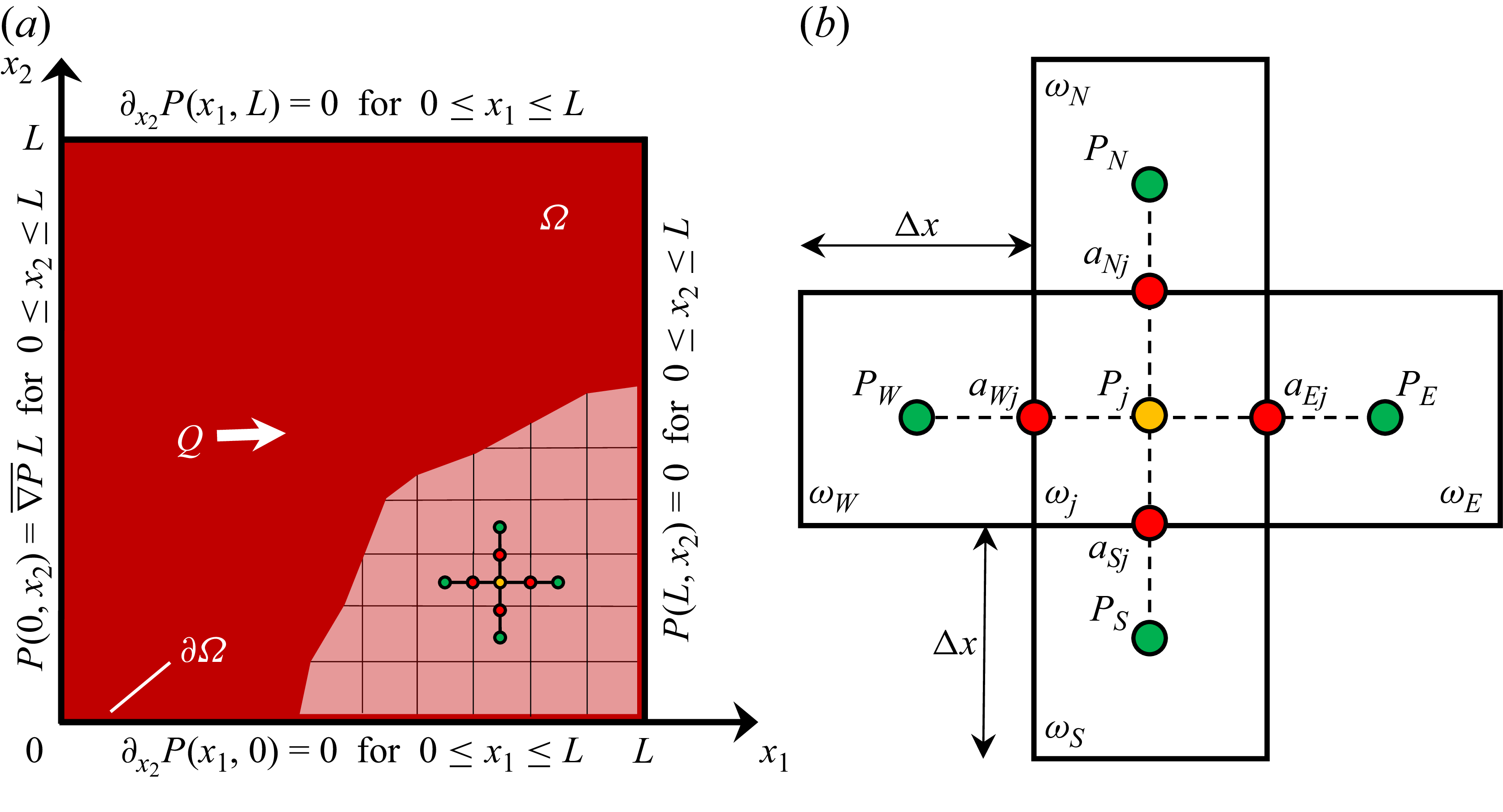
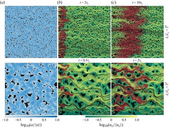
 107
107 t
t L/Lc=23
 25
25 σa/⟨a⟩=0.75
 Lc=0.1m
 ⟨a⟩=0.001m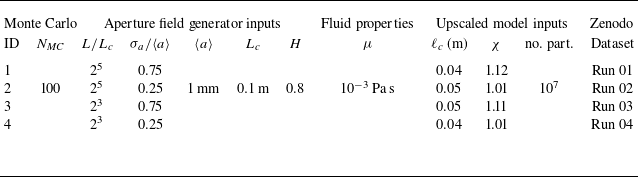
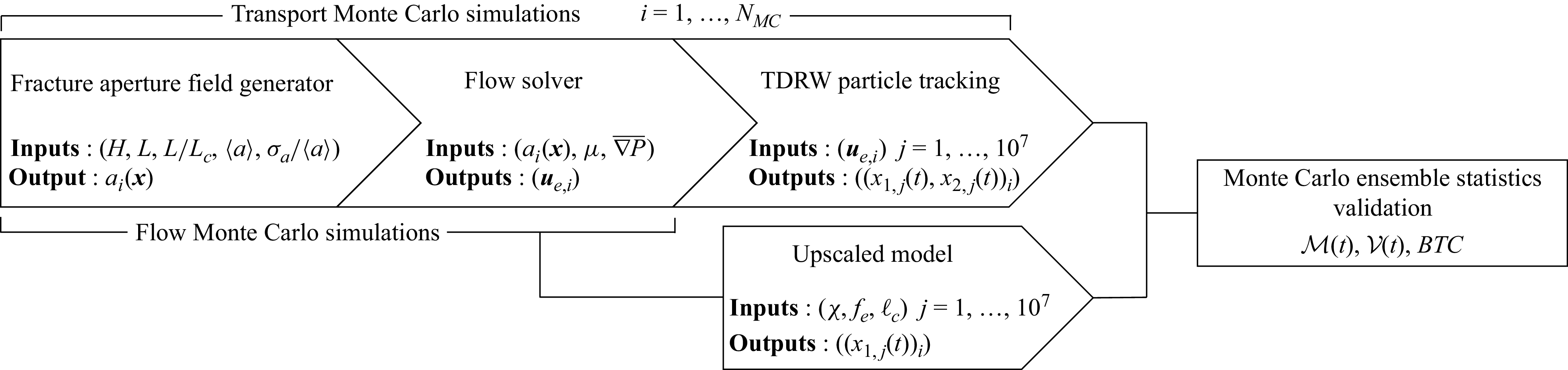

 s
s uα−1
uα−1 s
s uα
uα


 L
L Lc=0.1m
 L/Lc=25
 ⟨a⟩=0.001m
 α
α α=0.4
α=0.4 σa/⟨a⟩=0.75
 α=1
α=1 σa/⟨a⟩=0.25
 Open access

