





1. Introduction
Elastic loops, from a simple rubber band to the closed shells that encase soft actuators, combine the constraint of closed geometry with the compliance of a thin structure. This combination allows large shape change at modest energetic cost. Rich examples of mechanically driven deformations of elastic loops includes in-plane bending (Hazel & Mullin Reference Hazel and Mullin2017), out-of-plane bending (Davidovitch et al. Reference Davidovitch, Schroll, Vella, Adda-Bedia and Cerda2011; Box et al. Reference Box, Kodio, O’Kiely, Cantelli, Goriely and Vella2020), twisting (Goriely Reference Goriely2006), folding (Mouthuy et al. Reference Mouthuy, Coulombier, Pardoen, Raskin and Jonas2012; Lu et al. Reference Lu, Leanza, Dai, Hutchinson and Zhao2024) and even snap-through inversion (Yang et al. Reference Yang, Liu, Li, Xin and Dang2025). These versatile deformation modes suggest promising opportunities for adaptive morphing, which could be achieved by leveraging compliant closed-loop structures and actively controlling the morphology of the enclosing surfaces. While the effective control of compliant closed-loop structures demands precise manipulation of transient patterns, the development of a comprehensive methodology for generating diverse patterns on an elastic loop and elucidating the dynamics that govern them remains largely unexplored. Most prior studies on deformable elastic loops have instead focused on passive deformations driven by a surrounding fluid environment, such as flapping (Jung et al. Reference Jung, Mareck, Shelley and Zhang2006; Kim et al. Reference Kim, Huang, Shin and Sung2012) and sedimentation (Gruziel-Słomka et al. Reference Gruziel-Słomka, Kondratiuk, Szymczak and Ekiel-Jeżewska2019; Waszkiewicz, Szymczak & Lisicki Reference Waszkiewicz, Szymczak and Lisicki2021).
One promising approach for manipulating the shape changes of an elastic loop lies in applying surface instabilities such as wrinkling. Among various techniques for producing surface patterns, wrinkling based on elastic instability is particularly effective in generating complex and regular morphologies (Cerda & Mahadevan Reference Cerda and Mahadevan2003; Brojan et al. Reference Brojan, Terwagne, Lagrange and Reis2015). In addition to its use in measuring material properties (Stafford et al. Reference Stafford, Harrison, Beers, Karim, Amis, VanLandingham, Kim, Volksen, Miller and Simonyi2004; Chung, Nolte & Stafford Reference Chung, Nolte and Stafford2011), the reproducibility of wrinkling under well-defined geometrical and mechanical conditions enables precise control of surface topography (Chan et al. Reference Chan, Smith, Hayward and Crosby2008; Yang, Khare & Lin Reference Yang, Khare and Lin2010; Holmes & Crosby Reference Holmes and Crosby2010; Pocivavsek et al. Reference Pocivavsek, Pugar, O’Dea, Ye, Wagner, Tzeng, Velankar and Cerda2018; Liu et al. Reference Liu2019), thus serving as a bridge to drive three-dimensional morphing from two-dimensional configurations (Shim et al. Reference Shim, Perdigou, Chen, Bertoldi and Reis2012; Liu, Hacker & Daraio Reference Liu, Hacker and Daraio2021; Tanaka et al. Reference Tanaka, Montgomery, Yue, Wei, Song, Nomura and Qi2023).
On an elastic surface subjected to internal compression and buckling, wrinkle morphology emerges from the interplay between the resistance to bending and to transverse displacement (Cerda & Mahadevan Reference Cerda and Mahadevan2003). In particular, the deformation of an elastic loop under various buckling conditions has been addressed in classical elastica theory, and corresponding exact equilibrium profiles have been well established (Lévy Reference Lévy1884; Carrier Reference Carrier1947; Flaherty, Keller & Rubinow Reference Flaherty, Keller and Rubinow1972). Compared with quasi-static buckling systems (Mora et al. Reference Mora, Phou, Fromental, Audoly and Pomeau2012; Foster et al. Reference Foster, Verschueren, Knobloch and Gordillo2022), dynamic buckling provides access to a broader range of patterns, allowing higher modes of instability to occur without external constraints (Box et al. Reference Box, Kodio, O’Kiely, Cantelli, Goriely and Vella2020). Additionally, pattern selection can be readily tuned through system parameters, such as the impact speed of an external projectile onto a buckling structure (Gladden et al. Reference Gladden, Handzy, Belmonte and Villermaux2005; Vermorel, Vandenberghe & Villermaux Reference Vermorel, Vandenberghe and Villermaux2009). However, such parameter tuning is inherently an open-loop control problem, often requiring multiple trials to achieve the desired pattern. To mechanically guide the wrinkle patterns through dynamic interaction with the elastic loop, a comprehensive understanding of the effects of time-varying parameters is essential. These time-dependent parameters can reshape the spatiotemporal evolution of loop deformation in striking ways; for example, in the parametric resonance of an elastic loop, a spatially uniform yet temporally modulated stiffness can produce inhomogeneous large-amplitude responses (Cortez et al. Reference Cortez, Peskin, Stockie and Varela2004). This highlights how temporal modulation can strongly influence the dynamics of a deforming loop, offering insight into mechanically guided evolution of wrinkles.
In the context of wrinkling dynamics, a particularly relevant time-varying loading parameter is the external pressure applied to the elastic loop, which modulates the internal compressive force. The transient loading profile not only determines wrinkle localisation by competing with wave-propagation speed (Putelat & Triantafyllidis Reference Putelat and Triantafyllidis2014), but also influences the emergent mode number (Box et al. Reference Box, Kodio, O’Kiely, Cantelli, Goriely and Vella2020). However, in contrast to simple two-dimensional sheets (Wang et al. Reference Wang, Sun, He and Ni2023), experimental manifestations of transient loading effects on wrinkling in elastic loops are still lacking because it is technically challenging to impose a well-prescribed transient load on a closed-loop structure. Box et al. (Reference Box, Kodio, O’Kiely, Cantelli, Goriely and Vella2020) used the surface tension of a contacting soap film within a loop as a transient loading source. However, in that configuration, the loading process originates from the bursting of the soap film, so that the opening must propagate from the puncture point to the loop. The resulting loading may therefore contain an inherent azimuthal bias, which can promote the inhomogeneous growth of the instability on the loop. A complementary experimental approach that overcomes this difficulty and provides a more well-defined transient loading condition is needed as a testbed for studying the effects of transient loading on wrinkle dynamics.
In this paper, we investigate the hydrodynamic wrinkling of a circular elastic loop placed inside a Hele-Shaw type of apparatus. Because of the confined geometry of the apparatus, the transient radial gap flow generated by the motion of the apparatus applies nearly axisymmetric compressive loading prior to buckling, and the subsequent deformation of the loop induces the spatiotemporal redistribution of hydrodynamic pressure through fluid–structure interaction. This experimental platform facilitates the application of time-varying hydrodynamic forcing relevant to pattern formation (Ito Reference Ito1999; Chan & Crosby Reference Chan and Crosby2006; Xie, Luo & Gray Reference Xie, Luo and Gray2017), and reveals direct links between the transient characteristics of the hydrodynamic pressure and the resulting wrinkle geometry.
Section 2.1 describes the experimental set-up and the transient radial gap flow generated by the apparatus, and § 2.2 explains the loop fabrication process and relevant properties. In § 2.3, the transient hydrodynamic pressure acting on the loop is modelled by simulating radial flow around a fixed rigid loop as a surrogate system. A low-order numerical model that resolves loop deformation, while accounting for fluid–structure interaction, is then proposed in § 2.4. Using experimental and numerical results, the transient kinematics and mode selection mechanism of the loop are examined in § 3.1. Section 3.2 analyses wrinkle morphology in terms of the degree of which the pattern approaches a pure harmonic mode, and § 3.3 discusses an approach to mechanically guide a particular wrinkle pattern using spatially varying loop thickness. Concluding remarks are presented in § 4.
2. Problem description
2.1. Experimental set-up and radial gap flow distribution
A circular elastic loop was coaxially immersed in a water-filled gap between a stationary bottom substrate and a vertically translating cylindrical disk (figure 1 $a$
). The disk was translated by a linear guide vertically mounted to the disk. An incoming flow was generated by rapidly lifting the disk upwards according to the displacement profile
$a$
). The disk was translated by a linear guide vertically mounted to the disk. An incoming flow was generated by rapidly lifting the disk upwards according to the displacement profile $H(t)=H_{0}+A[1-\cos (2\pi t/T)]$
for
$H(t)=H_{0}+A[1-\cos (2\pi t/T)]$
for $t\leqslant T/2$
. After reaching a total displacement of
$t\leqslant T/2$
. After reaching a total displacement of $2A$
, the disk was kept stationary. The background flow in the absence of the loop was transient and axisymmetric, exhibiting a nearly uniform radial velocity profile (
$2A$
, the disk was kept stationary. The background flow in the absence of the loop was transient and axisymmetric, exhibiting a nearly uniform radial velocity profile ( $u_{r}$
) and a linear vertical velocity profile (
$u_{r}$
) and a linear vertical velocity profile ( $u_{z}$
) when the Reynolds number
$u_{z}$
) when the Reynolds number $Re = H_{0}\dot{H}_{\mathit{max}}/\nu$
is of
$Re = H_{0}\dot{H}_{\mathit{max}}/\nu$
is of $O(10^2)$
(figure 1
$O(10^2)$
(figure 1 $b$
); these velocity profiles were confirmed by the experiments that are described below.
$b$
); these velocity profiles were confirmed by the experiments that are described below.
( $a$
) Schematic of the experimental set-up. The gap distance
$a$
) Schematic of the experimental set-up. The gap distance $H(t)$
between the bottom substrate and the top disk is controlled by a linear guide (
$H(t)$
between the bottom substrate and the top disk is controlled by a linear guide ( $H_{0}=2.1$
–
$H_{0}=2.1$
– $5.0$
mm,
$5.0$
mm, $A=1.5$
–
$A=1.5$
– $3.6$
mm,
$3.6$
mm, $T=69$
–
$T=69$
– $135$
ms), and is measured with a laser displacement sensor. The wrinkling process is captured by a high-speed camera. (
$135$
ms), and is measured with a laser displacement sensor. The wrinkling process is captured by a high-speed camera. ( $b$
) Idealised profiles of normalised radial velocity
$b$
) Idealised profiles of normalised radial velocity $-u_{r}/U_{r}$
and normalised vertical velocity
$-u_{r}/U_{r}$
and normalised vertical velocity $u_{z}/\dot{H}$
of the incoming gap flow, in the absence of the elastic loop.
$u_{z}/\dot{H}$
of the incoming gap flow, in the absence of the elastic loop.

As a preliminary step towards understanding the fluid–structure interaction during the buckling of an elastic loop, we obtained the velocity field over time in the fluid domain between the moving disk and the bottom substrate, in the absence of the elastic loop, using particle image velocimetry. A high-speed camera (FASTCAM MINI-UX50, Photron, Inc.) was mounted in front of the water tank in which the substrate and the disk were submerged, and images were captured at 2000 frames per second. Hollow glass particles (Potters Industries LLC) with an average diameter of 11.7 $\unicode{x03BC}$
m and a density of 1.1 g ml
$\unicode{x03BC}$
m and a density of 1.1 g ml $^{-1}$
were seeded into the tank. A vertical laser sheet was generated by illuminating a plane including the central axis of the disk with a continuous laser (10 W, MGL-W-532A, CNI Co. Ltd). Image pairs were cross-correlated using a multi-grid interrogation method (PIVview2C 3.6, PIVTEC GmbH), starting with an initial window size of 128
$^{-1}$
were seeded into the tank. A vertical laser sheet was generated by illuminating a plane including the central axis of the disk with a continuous laser (10 W, MGL-W-532A, CNI Co. Ltd). Image pairs were cross-correlated using a multi-grid interrogation method (PIVview2C 3.6, PIVTEC GmbH), starting with an initial window size of 128 $\times$
128 pixels and refining to a final window size of 32
$\times$
128 pixels and refining to a final window size of 32 $\times$
32 pixels (50
$\times$
32 pixels (50 $\,\%$
overlap).
$\,\%$
overlap).
Two experimental conditions, $[H_{0}, A, T]$
= [3.0 mm, 1.1 mm, 208 ms] and [3.0 mm, 1.5 mm, 88 ms], were considered, corresponding to Reynolds numbers (
$[H_{0}, A, T]$
= [3.0 mm, 1.1 mm, 208 ms] and [3.0 mm, 1.5 mm, 88 ms], were considered, corresponding to Reynolds numbers ( $Re=H_{0}\dot{H}_{\mathit{max}}/\nu$
) of 100 and 321, respectively; these values are of
$Re=H_{0}\dot{H}_{\mathit{max}}/\nu$
) of 100 and 321, respectively; these values are of $O(10^2)$
, as required in the main experiments. Figure 2 shows velocity profiles in the radial (
$O(10^2)$
, as required in the main experiments. Figure 2 shows velocity profiles in the radial ( $u_{r}$
) and vertical (
$u_{r}$
) and vertical ( $u_{z}$
) directions over time at various radial positions
$u_{z}$
) directions over time at various radial positions $r$
. As the incoming flow develops under the action of the upper disk, the radial velocity becomes almost uniform (
$r$
. As the incoming flow develops under the action of the upper disk, the radial velocity becomes almost uniform ( $-u_{r}/U_{r}\approx 1$
), except at the top and bottom boundaries, for
$-u_{r}/U_{r}\approx 1$
), except at the top and bottom boundaries, for $2t/T\leqslant 0.75$
in both cases, while the vertical velocity tends to increase linearly with respect to
$2t/T\leqslant 0.75$
in both cases, while the vertical velocity tends to increase linearly with respect to $z$
(
$z$
( $u_{z}/\dot{H}=z/H$
). Velocity
$u_{z}/\dot{H}=z/H$
). Velocity $U_{r}=r\dot{H}/2H$
is the reference radial velocity of the flow, derived from the continuity condition for a cylindrical control volume of radius
$U_{r}=r\dot{H}/2H$
is the reference radial velocity of the flow, derived from the continuity condition for a cylindrical control volume of radius $r$
and height
$r$
and height $H$
. Here, the uniformity of the radial velocity is indicated by steep velocity gradients near the top and bottom boundaries and nearly constant velocity in the middle region. However, as
$H$
. Here, the uniformity of the radial velocity is indicated by steep velocity gradients near the top and bottom boundaries and nearly constant velocity in the middle region. However, as $\dot{H}$
decreases to 0 in
$\dot{H}$
decreases to 0 in $0.5\leqslant 2t/T\leqslant 1$
, the incoming flow decelerates to satisfy the continuity condition, reducing the radial velocity in the middle region to negative or near-zero values at
$0.5\leqslant 2t/T\leqslant 1$
, the incoming flow decelerates to satisfy the continuity condition, reducing the radial velocity in the middle region to negative or near-zero values at $2t/T\gt 0.75$
. Although fluid inertia makes the flow more complex during the deceleration stage, the transient gap flow can be regarded as nearly uniform in the radial direction and linear in the vertical direction prior to the post-buckling of the elastic loop, which is the focus of our study.
$2t/T\gt 0.75$
. Although fluid inertia makes the flow more complex during the deceleration stage, the transient gap flow can be regarded as nearly uniform in the radial direction and linear in the vertical direction prior to the post-buckling of the elastic loop, which is the focus of our study.
( $a$
) Normalised radial velocity
$a$
) Normalised radial velocity $-u_{r}/U_{r}$
and (
$-u_{r}/U_{r}$
and ( $b$
) normalised vertical velocity
$b$
) normalised vertical velocity $u_{z}/\dot{H}$
of the incoming gap flow, in the absence of the elastic loop, along the vertical direction at three instants; in each panel,
$u_{z}/\dot{H}$
of the incoming gap flow, in the absence of the elastic loop, along the vertical direction at three instants; in each panel, $[H_{0}, A, T]$
= [3.0 mm, 1.1 mm, 208 ms] (left) and [3.0 mm, 1.5 mm, 88 ms] (right). Squares, triangles and circles denote the radial positions
$[H_{0}, A, T]$
= [3.0 mm, 1.1 mm, 208 ms] (left) and [3.0 mm, 1.5 mm, 88 ms] (right). Squares, triangles and circles denote the radial positions $r=20$
, 30 and 40 mm, respectively.
$r=20$
, 30 and 40 mm, respectively.

2.2. Elastic loop fabrication and properties
As a result of the fluid–structure interaction, the elastic loop undergoes buckling, accompanied by an upward drift. In particular, the radial component ( $\boldsymbol{r}$
) of the gap flow generates a pressure difference between the inner and outer surfaces of the elastic loop, which in turn induces internal compression in the tangential direction (
$\boldsymbol{r}$
) of the gap flow generates a pressure difference between the inner and outer surfaces of the elastic loop, which in turn induces internal compression in the tangential direction ( $\boldsymbol{t}$
) and triggers the buckling of the loop (figure 3
$\boldsymbol{t}$
) and triggers the buckling of the loop (figure 3 $a$
) (Box et al. Reference Box, Kodio, O’Kiely, Cantelli, Goriely and Vella2020; Foster et al. Reference Foster, Verschueren, Knobloch and Gordillo2022). Because the aspect ratio between the thickness
$a$
) (Box et al. Reference Box, Kodio, O’Kiely, Cantelli, Goriely and Vella2020; Foster et al. Reference Foster, Verschueren, Knobloch and Gordillo2022). Because the aspect ratio between the thickness $w$
and the height
$w$
and the height $h$
of the loop is set to
$h$
of the loop is set to $w/h \lt 1$
, in-plane buckling occurs. A variety of wrinkle patterns are observed depending on the loop’s properties and the dynamic parameters, which have different numbers of wrinkle crests and troughs (figure 3
$w/h \lt 1$
, in-plane buckling occurs. A variety of wrinkle patterns are observed depending on the loop’s properties and the dynamic parameters, which have different numbers of wrinkle crests and troughs (figure 3 $b$
). Several elastic loops with different values of the diameter
$b$
). Several elastic loops with different values of the diameter $D$
, density
$D$
, density $\rho _{s}$
and Young’s modulus
$\rho _{s}$
and Young’s modulus $E$
were fabricated by mould casting of polydimethylsiloxane (PDMS).
$E$
were fabricated by mould casting of polydimethylsiloxane (PDMS).
( $a$
) Schematics of hydrodynamic wrinkling: initial geometry of the elastic loop before wrinkling (top) and buckled shape under the action of hydrodynamic pressure (bottom). (
$a$
) Schematics of hydrodynamic wrinkling: initial geometry of the elastic loop before wrinkling (top) and buckled shape under the action of hydrodynamic pressure (bottom). ( $b$
) Representative snapshots of wrinkle pattern. The corresponding parameter sets [
$b$
) Representative snapshots of wrinkle pattern. The corresponding parameter sets [ $D$
,
$D$
, $H_{0}$
,
$H_{0}$
, $A$
,
$A$
, $T$
] are (i) [40, 2.2, 2.9 mm, 133 ms], (ii) [50, 2.1, 2.4 mm, 81 ms], (iii) [80, 2.8, 3.0 mm, 83 ms] and (iv) [90, 2.3, 2.9 mm, 82 ms]; see table 1 for loop properties.
$T$
] are (i) [40, 2.2, 2.9 mm, 133 ms], (ii) [50, 2.1, 2.4 mm, 81 ms], (iii) [80, 2.8, 3.0 mm, 83 ms] and (iv) [90, 2.3, 2.9 mm, 82 ms]; see table 1 for loop properties.

To make an elastic loop with a rectangular cross-section, we used a mould-casting technique based on the temperature-dependent curing property of PDMS. An acrylic mould was pre-assembled with the layers of laser-cut acrylic plates. A mix ratio of 10:1 between the base and the curing agent (Sylgard 184, Dow Corning Ltd) was chosen, and the mixture was poured into the acrylic mould after 5 min of stirring. To eliminate gas bubbles, the sample was depressurised in a vacuum chamber, and an acrylic lid component was placed on the sample to cover the exposed top. Depressurisation was repeated to remove additional gas bubbles that might have formed when covering the exposed top. The curing time and temperature of the oven were set to 1 h and $100\,^\circ \textrm {C}$
, and the sample was removed from the oven to be cooled at room temperature
$100\,^\circ \textrm {C}$
, and the sample was removed from the oven to be cooled at room temperature $(25\,^\circ \textrm {C})$
.
$(25\,^\circ \textrm {C})$
.
The mechanical properties of the elastic loop were required for our analysis. Thus, we constructed a tensile testing device that can apply extension to the elastic loop and measure the stress for a given strain. The tensile testing device in figure 4 held each side of the loop with cylindrical pins when extension was applied. A linear guide provided the displacement required for the extension of the loop, while a fixed load cell (MBP-5, Interface, Inc.) was connected to the other side of the loop to measure the applied load. During the measurement, the distance between the two ends was steadily increased such that only a static load was in effect. Here, the Poisson’s ratio was not directly measured and was approximated as $\nu =0.49$
, which is reasonable considering that the Poisson’s ratio of PDMS is reportedly 0.49 for strain below 45 % (Johnston et al. Reference Johnston, McCluskey, Tan and Tracey2014).
$\nu =0.49$
, which is reasonable considering that the Poisson’s ratio of PDMS is reportedly 0.49 for strain below 45 % (Johnston et al. Reference Johnston, McCluskey, Tan and Tracey2014).
(a) Schematic of the tensile testing device and (b) force–distance data for elastic loops with different diameters $D$
. The measured data are plotted with square markers, and the corresponding linear fits (2.1) are shown as solid lines.
$D$
. The measured data are plotted with square markers, and the corresponding linear fits (2.1) are shown as solid lines.

By deriving the relation between the applied load $F$
on the load cell and the distance
$F$
on the load cell and the distance $l$
between the two ends, the elastic modulus of the elastic loop was estimated. In figure 4, the loop with cross-sectional area
$l$
between the two ends, the elastic modulus of the elastic loop was estimated. In figure 4, the loop with cross-sectional area $S=wh$
deforms under
$S=wh$
deforms under $F/2$
, resulting in an elongation of strain
$F/2$
, resulting in an elongation of strain $\epsilon =(l+\pi a-\pi D/2)/(\pi D/2)$
, where
$\epsilon =(l+\pi a-\pi D/2)/(\pi D/2)$
, where $D$
is the initial diameter of the loop and
$D$
is the initial diameter of the loop and $a$
is the radius of the cylindrical pins. Following the linear elasticity relation, the stress is represented as
$a$
is the radius of the cylindrical pins. Following the linear elasticity relation, the stress is represented as $\sigma =E\epsilon$
, where
$\sigma =E\epsilon$
, where $E$
is the elastic modulus. Because
$E$
is the elastic modulus. Because $F/2=\sigma S$
, the applied load is given by
$F/2=\sigma S$
, the applied load is given by $F=2Ewh\epsilon$
. By substituting
$F=2Ewh\epsilon$
. By substituting $\epsilon =(l+\pi a-\pi D/2)/(\pi D/2)$
, the following relation was obtained:
$\epsilon =(l+\pi a-\pi D/2)/(\pi D/2)$
, the following relation was obtained:
 \begin{equation} F(l)=2Ewh\left [\frac {2(l/\pi +a)}{D}-1\right ]. \end{equation}
The elastic modulus was then extracted from the measured $F$
and
$F$
and $l$
. The models and their properties used in the experiments are summarised in table 1.
$l$
. The models and their properties used in the experiments are summarised in table 1.
Properties of elastic loops with uniform thickness used in the experiments. The elastic modulus of loops with non-uniform thickness was not measured and is therefore not included. The height of the loop is $h=2$
mm.
$h=2$
mm.

Table 1. Long description
The table presents properties of elastic loops with uniform thickness used in experiments. It includes seven models with varying diameters, thicknesses, elastic moduli, and densities. The diameter ranges from 30 to 90 millimeters, thickness from 1.1 to 1.3 millimeters, elastic modulus from 0.76 to 1.37 megapascals, and density from 870 to 998 kilograms per cubic meter. The elastic modulus of loops with non-uniform thickness was not measured and is therefore not included. The height of the loop is in millimeters.
2.3. Model of transient hydrodynamic pressure
The dynamic buckling of an elastic loop introduces a complex fluid–structure interaction and eventually leads to asymmetric gap flow. Moreover, the local motion of a loop segment per unit length, which is described in figure 5, alleviates the hydrodynamic pressure difference between the inner and outer sides of the loop segment, and creates an asymmetric pressure field with respect to the $z$
axis. To simplify the problem, the asymmetric flow can be divided into the undisturbed flow component, which arises when the loop is assumed to be rigid with no deformation, and the disturbed flow component due to the deformation of the elastic loop. For a fixed rigid loop, the loop geometry remains axisymmetric, and the resultant undisturbed flow is assumed to be axisymmetric. Although asymmetric components arise in the hydrodynamic pressure of an elastic loop, they are not significant during the early stage of buckling when the deformation is small. The undisturbed axisymmetric pressure associated with a fixed rigid loop can be regarded as an effective pressure scale governing the instantaneous hydrodynamic loading responsible for wrinkle formation in the elastic loop. To reduce the complexity of the analysis, we first model this undisturbed axisymmetric pressure in this section. Then, a low-order numerical model that accounts for spatiotemporal variations in the pressure along the circumference of the deforming loop is presented in § 2.4.
$z$
axis. To simplify the problem, the asymmetric flow can be divided into the undisturbed flow component, which arises when the loop is assumed to be rigid with no deformation, and the disturbed flow component due to the deformation of the elastic loop. For a fixed rigid loop, the loop geometry remains axisymmetric, and the resultant undisturbed flow is assumed to be axisymmetric. Although asymmetric components arise in the hydrodynamic pressure of an elastic loop, they are not significant during the early stage of buckling when the deformation is small. The undisturbed axisymmetric pressure associated with a fixed rigid loop can be regarded as an effective pressure scale governing the instantaneous hydrodynamic loading responsible for wrinkle formation in the elastic loop. To reduce the complexity of the analysis, we first model this undisturbed axisymmetric pressure in this section. Then, a low-order numerical model that accounts for spatiotemporal variations in the pressure along the circumference of the deforming loop is presented in § 2.4.
Schematic of the gap flow induced by the disk moving upwards. An enlarged image near the elastic loop is depicted inside the red dashed box. In the box, velocity profiles of undisturbed flow (for a fixed rigid loop) and disturbed flow (for a deforming elastic loop) are denoted by the dashed and solid lines, respectively.

By treating the elastic loop as rigid and conducting simple simulations that compute the axisymmetric undisturbed gap flow, the scale of the transient hydrodynamic pressure acting on the elastic loop can be estimated. By virtue of the axisymmetric assumption, a reduced computational fluid domain was constructed in a two-dimensional domain composed of the radial ( $r$
) and vertical (
$r$
) and vertical ( $z$
) coordinates. The radial length and vertical height of the computational domain were set to 150 and 40 mm, respectively (figure 6). A no-slip condition for the velocity and a zero gradient in the normal direction for the pressure were imposed on the bottom (substrate surface) and the surfaces of the loop. The other boundaries, except the axisymmetric
$z$
) coordinates. The radial length and vertical height of the computational domain were set to 150 and 40 mm, respectively (figure 6). A no-slip condition for the velocity and a zero gradient in the normal direction for the pressure were imposed on the bottom (substrate surface) and the surfaces of the loop. The other boundaries, except the axisymmetric $z$
axis, were assigned a zero-gradient velocity in the normal direction and zero pressure.
$z$
axis, were assigned a zero-gradient velocity in the normal direction and zero pressure.
For the fluid solver, the incompressible PISO algorithm in OpenFOAM was adopted to solve the following mass and momentum conservation equations:
 \begin{align} \boldsymbol{\nabla }\boldsymbol{\cdot }\boldsymbol{u} & = 0, \end{align}
 \begin{align} \frac {\partial \boldsymbol{u}}{\partial t} + \boldsymbol{\nabla }\boldsymbol{\cdot }(\boldsymbol{u} \boldsymbol{u}) & = -\frac {1}{\rho _f} \boldsymbol{\nabla }p + \nu {\boldsymbol{\nabla} }^2\boldsymbol{u}, \end{align}
( $a$
) Fluid domain with background grid and boundary conditions and (b) background grid layout. The black dashed box in (
$a$
) Fluid domain with background grid and boundary conditions and (b) background grid layout. The black dashed box in ( $a$
) depicts the domain near the rigid loop, and the black rectangle inside region I of (b) denotes the loop. (c) Fluid domain near the moving disk with dynamic grid and boundary conditions and (d) dynamic grid layout.
$a$
) depicts the domain near the rigid loop, and the black rectangle inside region I of (b) denotes the loop. (c) Fluid domain near the moving disk with dynamic grid and boundary conditions and (d) dynamic grid layout.

where $\boldsymbol{u}$
,
$\boldsymbol{u}$
, $p$
,
$p$
, $\rho _{f}$
and
$\rho _{f}$
and $\nu$
denote the fluid velocity, pressure, density and kinematic viscosity, respectively. In this study, the fluid density and kinematic viscosity were held constant at values of
$\nu$
denote the fluid velocity, pressure, density and kinematic viscosity, respectively. In this study, the fluid density and kinematic viscosity were held constant at values of $\rho _{f}=1.0\times 10^3$
kg m
$\rho _{f}=1.0\times 10^3$
kg m $^{-3}$
and
$^{-3}$
and $\nu =8.9\times 10^{-7}$
m
$\nu =8.9\times 10^{-7}$
m $^2$
s
$^2$
s $^{-1}$
. For the discretisation of the temporal derivative term, the implicit Euler scheme was applied. The Gauss linear scheme was employed to discretise the spatial derivative terms.
$^{-1}$
. For the discretisation of the temporal derivative term, the implicit Euler scheme was applied. The Gauss linear scheme was employed to discretise the spatial derivative terms.
The displacement profiles of the disk were set to $H(t)=H_{0}+A[1-\cos (2\pi t/T)]$
, and the disk remained stationary at
$H(t)=H_{0}+A[1-\cos (2\pi t/T)]$
, and the disk remained stationary at $H= H_0+ 2A$
for
$H= H_0+ 2A$
for $t\gt T/2$
. However, because the sinusoidal profile causes a discontinuous hydrodynamic force at
$t\gt T/2$
. However, because the sinusoidal profile causes a discontinuous hydrodynamic force at $t=0$
s due to the non-zero initial acceleration, the smooth profiles measured in the experiments were used in the simulations. The simulations were conducted for several periods
$t=0$
s due to the non-zero initial acceleration, the smooth profiles measured in the experiments were used in the simulations. The simulations were conducted for several periods $T=[0.13$
–
$T=[0.13$
– $0.28]$
s and loop diameters
$0.28]$
s and loop diameters $D=[60, 80]$
mm, while the initial gap distance and the amplitude of the motion were fixed to
$D=[60, 80]$
mm, while the initial gap distance and the amplitude of the motion were fixed to $H_{0}=3$
mm and
$H_{0}=3$
mm and $A=2$
mm, respectively. In addition, to account for the experimentally observed vertical displacement of the loop (
$A=2$
mm, respectively. In addition, to account for the experimentally observed vertical displacement of the loop ( $\Delta z\lesssim 3(H_{0}-h)/4$
), the rigid loop was fixed at the centre of the initial gap,
$\Delta z\lesssim 3(H_{0}-h)/4$
), the rigid loop was fixed at the centre of the initial gap, $z = H_{0}/2$
. Preliminary simulations comparing the net hydrodynamic pressure acting on a rigid loop fixed at different vertical positions showed that the transient pressure profile is not distinctly affected by moderate variations in the vertical position of the loop. Accordingly,
$z = H_{0}/2$
. Preliminary simulations comparing the net hydrodynamic pressure acting on a rigid loop fixed at different vertical positions showed that the transient pressure profile is not distinctly affected by moderate variations in the vertical position of the loop. Accordingly, $z = H_{0}/2$
was adopted as a representative vertical position for the simulations.
$z = H_{0}/2$
was adopted as a representative vertical position for the simulations.
To implement the moving boundary of the disk in the simulations, overset grids were constructed by merging a stationary background grid and a dynamic grid. In figure 6(c,d), the moving disk (with radial length of 75 mm and vertical height of 10 mm) is included in the dynamic grid, which moves in the stationary background grid during the simulation. At the beginning of each time step, $\boldsymbol{u}$
and
$\boldsymbol{u}$
and $p$
were interpolated from the background grid to the boundaries of the dynamic grid. Simultaneously, the values of
$p$
were interpolated from the background grid to the boundaries of the dynamic grid. Simultaneously, the values of $\boldsymbol{u}$
and
$\boldsymbol{u}$
and $p$
on the disk were interpolated from the boundaries of the dynamic grid to the background grid. The interpolation weights were calculated using the inverse of the distance between the adjacent cell of the dynamic grid and the interpolated cell of the background grid (and vice versa). The interpolation results were then used to solve the mass and momentum conservation equations (2.2a
)–(2.2b
) in both the background and dynamic grids.
$p$
on the disk were interpolated from the boundaries of the dynamic grid to the background grid. The interpolation weights were calculated using the inverse of the distance between the adjacent cell of the dynamic grid and the interpolated cell of the background grid (and vice versa). The interpolation results were then used to solve the mass and momentum conservation equations (2.2a
)–(2.2b
) in both the background and dynamic grids.
The background grid in the regions near the loop (I–III) and the dynamic grid in this study were composed of uniform cells obtained from multiple refinements (figure 6). Region I is the reference grid with the finest cell size of 25 $\unicode{x03BC}$
m, and the cells are coarsened to 50
$\unicode{x03BC}$
m, and the cells are coarsened to 50 $\unicode{x03BC}$
m (region II) and 100
$\unicode{x03BC}$
m (region II) and 100 $\unicode{x03BC}$
m (region III). Regions I–III in the dynamic grid have identical cell sizes to the corresponding regions I–III in the background grid, thus reducing the interpolation error. A non-uniform grid was employed in regions far from the loop (IV and V) to reduce the computational cost. The cell size in region IV on the right and upper side of the uniform grid (figure 6
$\unicode{x03BC}$
m (region III). Regions I–III in the dynamic grid have identical cell sizes to the corresponding regions I–III in the background grid, thus reducing the interpolation error. A non-uniform grid was employed in regions far from the loop (IV and V) to reduce the computational cost. The cell size in region IV on the right and upper side of the uniform grid (figure 6 $a{,}b$
) expands from 100
$a{,}b$
) expands from 100 $\unicode{x03BC}$
m in the radial and vertical directions, respectively. The size of the largest cell is four times greater than that of the coarsest uniform cell (100
$\unicode{x03BC}$
m in the radial and vertical directions, respectively. The size of the largest cell is four times greater than that of the coarsest uniform cell (100 $\unicode{x03BC}$
m). Region V consists of cells expanding in both the radial and vertical directions, and the expansion ratio is the same as that in region IV.
$\unicode{x03BC}$
m). Region V consists of cells expanding in both the radial and vertical directions, and the expansion ratio is the same as that in region IV.
A grid convergence test was conducted to determine appropriate cell sizes. The cell sizes in region I were $\Delta x=[30, 25, 17, 12.5]$ $\unicode{x03BC}$
m for the four test cases. In each case, the radial force per unit length,
$\unicode{x03BC}$
m for the four test cases. In each case, the radial force per unit length, $F_r$
(N m
$F_r$
(N m $^{-1}$
), acting on the loop was calculated for the input parameters
$^{-1}$
), acting on the loop was calculated for the input parameters $T=0.13$
s and
$T=0.13$
s and $D=80$
mm. The time histories of the negative radial force per unit length,
$D=80$
mm. The time histories of the negative radial force per unit length, $-F_r$
, feature the overall increase, reaching a global maximum, and the subsequent decrease. In figure 7(
$-F_r$
, feature the overall increase, reaching a global maximum, and the subsequent decrease. In figure 7( $a$
), the magnitudes of
$a$
), the magnitudes of $F_r$
at the global maximum are compared for the four cases. We confirmed that the numerical results converged in
$F_r$
at the global maximum are compared for the four cases. We confirmed that the numerical results converged in $\Delta x\leqslant 25$ $\unicode{x03BC}$
m with an error of less than 0.7 %. Accordingly, the cell size in region I was set to
$\unicode{x03BC}$
m with an error of less than 0.7 %. Accordingly, the cell size in region I was set to $\Delta x=25$ $\unicode{x03BC}$
m in all the simulations.
$\unicode{x03BC}$
m in all the simulations.
( $a$
) Grid convergence test: global maximum of the radial force magnitude per unit length,
$a$
) Grid convergence test: global maximum of the radial force magnitude per unit length, $|F_r|_{\mathit{max}}$
, acting on the rigid loop for four cases with different cell sizes (
$|F_r|_{\mathit{max}}$
, acting on the rigid loop for four cases with different cell sizes ( $T=0.13$
s and
$T=0.13$
s and $D=80$
mm). (
$D=80$
mm). ( $b$
) Validation: temporal evolution of the vertical force
$b$
) Validation: temporal evolution of the vertical force $F_z$
acting on the moving disk from the experiment and simulation (
$F_z$
acting on the moving disk from the experiment and simulation ( $T=0.33$
s).
$T=0.33$
s).

The time step was adjusted by setting the maximum Courant–Friedrichs–Lewy (CFL) number to a target value. The initial time step was $10$
$10$ $\unicode{x03BC}$
s, while the target CFL number was determined through a preliminary test by varying the target CFL number between 0.125 and 0.50. The differences in the magnitude of
$\unicode{x03BC}$
s, while the target CFL number was determined through a preliminary test by varying the target CFL number between 0.125 and 0.50. The differences in the magnitude of $F_r$
at the global maximum among the cases were less than 0.3 %. Thus, the target CFL number for the simulations was fixed to 0.50 in this study.
$F_r$
at the global maximum among the cases were less than 0.3 %. Thus, the target CFL number for the simulations was fixed to 0.50 in this study.
The numerical method was validated by comparing the vertical force $F_z$
(N) acting on the moving disk between the experimental and simulation results when there is no loop in the gap;
$F_z$
(N) acting on the moving disk between the experimental and simulation results when there is no loop in the gap; $T=0.33$
s. In the experiment, a load cell (MBP-5, Interface, Inc.) was installed between the linear guide and the disk to measure the vertical hydrodynamic load exerted on the moving disk. Because the hydrodynamic force varies rapidly over time, the load cell response exhibits a finite dynamic delay that must be corrected. We therefore applied a correction based on the mass–spring–damper model of the load cell, such that
$T=0.33$
s. In the experiment, a load cell (MBP-5, Interface, Inc.) was installed between the linear guide and the disk to measure the vertical hydrodynamic load exerted on the moving disk. Because the hydrodynamic force varies rapidly over time, the load cell response exhibits a finite dynamic delay that must be corrected. We therefore applied a correction based on the mass–spring–damper model of the load cell, such that $(1/\omega _{n}^2)\ddot {F}_{z}+(2\zeta /\omega _{n})\dot{F}_{z}+F_{z}=F_{z,c}$
, where
$(1/\omega _{n}^2)\ddot {F}_{z}+(2\zeta /\omega _{n})\dot{F}_{z}+F_{z}=F_{z,c}$
, where $F_{z}(t)$
is the measured force and
$F_{z}(t)$
is the measured force and $F_{z,c}(t)$
is the corrected force. The natural frequency
$F_{z,c}(t)$
is the corrected force. The natural frequency $\omega _{n}$
and damping ratio
$\omega _{n}$
and damping ratio $\zeta$
were obtained from a separate calibration experiment in which the step response of the load cell was measured and fitted to the analytical solution of a mass–spring–damper system. This procedure yielded
$\zeta$
were obtained from a separate calibration experiment in which the step response of the load cell was measured and fitted to the analytical solution of a mass–spring–damper system. This procedure yielded $\omega _{n}=71.7$
s
$\omega _{n}=71.7$
s $^{-1}$
and
$^{-1}$
and $\zeta =0.675$
. In the simulation, the vertical force acting on the disk was obtained by multiplying the vertical force per unit area by the disk area. According to figure 7(
$\zeta =0.675$
. In the simulation, the vertical force acting on the disk was obtained by multiplying the vertical force per unit area by the disk area. According to figure 7( $b$
), the simulation result is in good agreement with the experimental result.
$b$
), the simulation result is in good agreement with the experimental result.
The net hydrodynamic pressure $\bar {p}_{\mathit{und}}$
(where the subscript ‘und’ denotes the undisturbed axisymmetric pressure associated with the fixed rigid loop) between the inner and outer surfaces of the elastic loop is then estimated based on the aforementioned numerical simulations. The time evolution of the hydrodynamic pressure is then obtained from the simulation results. In figure 8(
$\bar {p}_{\mathit{und}}$
(where the subscript ‘und’ denotes the undisturbed axisymmetric pressure associated with the fixed rigid loop) between the inner and outer surfaces of the elastic loop is then estimated based on the aforementioned numerical simulations. The time evolution of the hydrodynamic pressure is then obtained from the simulation results. In figure 8( $a$
), an area of lower negative (gauge) pressure appears in the wake (inner) region of the loop, causing a pressure difference between the inner and outer regions of the loop. The radial hydrodynamic force per unit circumferential length,
$a$
), an area of lower negative (gauge) pressure appears in the wake (inner) region of the loop, causing a pressure difference between the inner and outer regions of the loop. The radial hydrodynamic force per unit circumferential length, $F_{r}$
, is composed of a pressure force component and a friction force component. The rectangular geometry of the loop’s cross-section means that the pressure force component corresponds to the radial force acting on the inner and outer surfaces normal to the
$F_{r}$
, is composed of a pressure force component and a friction force component. The rectangular geometry of the loop’s cross-section means that the pressure force component corresponds to the radial force acting on the inner and outer surfaces normal to the $r$
direction, whereas the friction force component corresponds to the radial force acting on the top and bottom surfaces normal to the
$r$
direction, whereas the friction force component corresponds to the radial force acting on the top and bottom surfaces normal to the $z$
direction. According to the simulations, the magnitude of the pressure force component is
$z$
direction. According to the simulations, the magnitude of the pressure force component is $O(10^{2})$
times that of the friction force component.
$O(10^{2})$
times that of the friction force component.
( $a$
) Pressure fields and streamlines near the rigid loop (corresponding to the dashed box in figure 5) at
$a$
) Pressure fields and streamlines near the rigid loop (corresponding to the dashed box in figure 5) at $t/T=0.16$
:
$t/T=0.16$
: $D=80$
mm,
$D=80$
mm, $T=0.13$
s (left) and
$T=0.13$
s (left) and $D=60$
mm,
$D=60$
mm, $T=0.14$
s (right). (
$T=0.14$
s (right). ( $b$
) Net hydrodynamic pressure
$b$
) Net hydrodynamic pressure $\bar {p}_{\mathit{und}}$
acting on the rigid loop during a loading cycle of the gap flow. The solid lines denote the simulation results and the dashed lines denote the scaled values
$\bar {p}_{\mathit{und}}$
acting on the rigid loop during a loading cycle of the gap flow. The solid lines denote the simulation results and the dashed lines denote the scaled values $\bar {p}_{\mathit{und}}= ({1}/{2})C_{D}\rho _{f}U^2$
in (2.3):
$\bar {p}_{\mathit{und}}= ({1}/{2})C_{D}\rho _{f}U^2$
in (2.3): $D=80$
mm (left) and
$D=80$
mm (left) and $D=60$
mm (right). (
$D=60$
mm (right). ( $c$
) Drag coefficient
$c$
) Drag coefficient $C_D$
with respect to period
$C_D$
with respect to period $T$
, corresponding to each case in (
$T$
, corresponding to each case in ( $b$
). (
$b$
). ( $d$
) Time history of
$d$
) Time history of $\bar {p}_{\mathit{und}}$
modelled as (2.3) for a sinusoidal
$\bar {p}_{\mathit{und}}$
modelled as (2.3) for a sinusoidal $H(t)$
profile:
$H(t)$
profile: $H=H_0+A[1-\cos (2\pi t/T)]$
.
$H=H_0+A[1-\cos (2\pi t/T)]$
.

Using the reference dynamic pressure $({1}/{2})\rho _{f}U^2$
, the value of
$({1}/{2})\rho _{f}U^2$
, the value of $-F_r$
(radial force in the inward direction) can be expressed as
$-F_r$
(radial force in the inward direction) can be expressed as $-F_r = ({1}/{2})C_D \rho _{f}U^2h$
, where
$-F_r = ({1}/{2})C_D \rho _{f}U^2h$
, where $C_D$
and
$C_D$
and $U$
denote the drag coefficient and reference flow velocity, respectively, and
$U$
denote the drag coefficient and reference flow velocity, respectively, and $\rho _{f}$
is the fluid density. To define
$\rho _{f}$
is the fluid density. To define $U$
, we consider the mass balance in the control volume enclosed by a cylindrical surface that has diameter
$U$
, we consider the mass balance in the control volume enclosed by a cylindrical surface that has diameter $D$
and height
$D$
and height $H(t)$
. The rate of volumetric flux entrained into the control volume is
$H(t)$
. The rate of volumetric flux entrained into the control volume is $\pi D^2\dot{H}/4=\pi D(H-h)U$
, yielding
$\pi D^2\dot{H}/4=\pi D(H-h)U$
, yielding $U=D\dot{H}/[4(H-h)]$
. The net hydrodynamic pressure acting on the loop in the radial direction,
$U=D\dot{H}/[4(H-h)]$
. The net hydrodynamic pressure acting on the loop in the radial direction, $\bar {p}_{\mathit{und}}\ (=-F_r/h)$
, is modelled as
$\bar {p}_{\mathit{und}}\ (=-F_r/h)$
, is modelled as
 \begin{equation} \bar {p}_{\mathit{und}}= \frac {1}{2}C_D \rho _{f}U^2 = \frac {1}{2}C_D \rho _{f} \left (\frac {D\dot{H}}{4(H-h)}\right )^2, \end{equation}
which provides a reasonable match with the simulation results in figure 8( $b$
). Even without considering the effect of added mass force due to flow acceleration separately, the net hydrodynamic force can be modelled reasonably based on (2.3). The ratio of the maximum of the added mass force (
$b$
). Even without considering the effect of added mass force due to flow acceleration separately, the net hydrodynamic force can be modelled reasonably based on (2.3). The ratio of the maximum of the added mass force ( $\sim \rho _fhw\dot{U}$
) to the maximum of the drag force (
$\sim \rho _fhw\dot{U}$
) to the maximum of the drag force ( $({1}/{2})C_D\rho _fhU^2$
) scales as
$({1}/{2})C_D\rho _fhU^2$
) scales as $\mathrm{max}(w\dot{U})/\mathrm{max}(U^2)\sim w/D$
, which just has an order of magnitude
$\mathrm{max}(w\dot{U})/\mathrm{max}(U^2)\sim w/D$
, which just has an order of magnitude $O(10^{-2})$
.
$O(10^{-2})$
.
The drag coefficient $C_{D}$
in (2.3) is obtained from the ratio between the maximum pressure calculated from the simulations and the maximum of
$C_{D}$
in (2.3) is obtained from the ratio between the maximum pressure calculated from the simulations and the maximum of $({1}/{2})\rho _{f}U^2$
; this quantity is plotted in figure 8(
$({1}/{2})\rho _{f}U^2$
; this quantity is plotted in figure 8( $c$
). Drag coefficient
$c$
). Drag coefficient $C_{D}$
ranges between 2.0 and 2.3 depending on the variations in the period
$C_{D}$
ranges between 2.0 and 2.3 depending on the variations in the period $T$
. As the differences in
$T$
. As the differences in $C_{D}$
are minor and the absolute value of
$C_{D}$
are minor and the absolute value of $C_{D}$
is insignificant in the analysis, it is acceptable to use the averaged value
$C_{D}$
is insignificant in the analysis, it is acceptable to use the averaged value $C_{D}=2.18$
for every case considered in this study. For the sinusoidal profile of
$C_{D}=2.18$
for every case considered in this study. For the sinusoidal profile of $H(t)$
, the pressure
$H(t)$
, the pressure $\bar {p}_{\mathit{und}}(t)$
exhibits a bell-shaped temporal profile that is skewed to the right (figure 8
$\bar {p}_{\mathit{und}}(t)$
exhibits a bell-shaped temporal profile that is skewed to the right (figure 8 $d$
). The characteristic parameters describing this transient pressure profile are expressed as
$d$
). The characteristic parameters describing this transient pressure profile are expressed as
 \begin{align} \bar {p}_{\mathit{max}}&=\frac {\pi ^2C_{D}\rho _{f}D^2}{8\alpha (\alpha +2)T^2}, \end{align}
 \begin{align} t_{P}&=\frac {T}{2\pi }\tan ^{-1}[\alpha ^{1/2}(\alpha +2)^{1/2}], \end{align}
 \begin{align} \Delta t_{P/2}&=\frac {T}{2\pi }\left [ \cos ^{-1}\left (\frac {1+\alpha -\sqrt {2}\alpha (\alpha +2)}{2\alpha (\alpha +2)+1}\right ) - \cos ^{-1}\left (\frac {1+\alpha +\sqrt {2}\alpha (\alpha +2)}{2\alpha (\alpha +2)+1}\right ) \right ], \end{align}
where $\bar {p}_{\mathit{max}}$
is the peak magnitude,
$\bar {p}_{\mathit{max}}$
is the peak magnitude, $t_{P}$
is the instant of the pressure peak and
$t_{P}$
is the instant of the pressure peak and $\Delta t_{P/2}$
is the duration of the pressure profile between the two instants corresponding to
$\Delta t_{P/2}$
is the duration of the pressure profile between the two instants corresponding to $\bar {p}_{\mathit{max}}/2$
(figure 8
$\bar {p}_{\mathit{max}}/2$
(figure 8 $d$
); here,
$d$
); here, $\alpha =(H_{0}-h)/A$
. As the skewness of the pressure profile depends on the ratio of the peak time to the time interval of loading, namely
$\alpha =(H_{0}-h)/A$
. As the skewness of the pressure profile depends on the ratio of the peak time to the time interval of loading, namely $t_{P}/(T/2)=\tan ^{-1}[\alpha ^{1/2}(\alpha +2)^{1/2}]/\pi$
, the pressure profile in figure 8(
$t_{P}/(T/2)=\tan ^{-1}[\alpha ^{1/2}(\alpha +2)^{1/2}]/\pi$
, the pressure profile in figure 8( $d$
) becomes more symmetric (i.e. less skewed) as
$d$
) becomes more symmetric (i.e. less skewed) as $\alpha$
increases.
$\alpha$
increases.
2.4. Low-order numerical model for fluid–structure interaction of the loop
With the transient hydrodynamic pressure profile characterised, low-order numerical simulations of the wrinkling of an elastic loop are conducted by solving Kirchhoff’s equation (Audoly & Pomeau Reference Audoly and Pomeau2010; Kodio, Goriely & Vella Reference Kodio, Goriely and Vella2020). In the low-order numerical model, spatiotemporal variation in hydrodynamic pressure along the loop should be accounted for to reflect the fluid–structure interaction arising during the wrinkling process. Figure 9( $a$
) depicts the elastic loop undergoing deformation due to net hydrodynamic pressure
$a$
) depicts the elastic loop undergoing deformation due to net hydrodynamic pressure $\bar {p}$
between the inner and outer surfaces, where the subscript ‘und’ is dropped to distinguish it from the spatially uniform pressure
$\bar {p}$
between the inner and outer surfaces, where the subscript ‘und’ is dropped to distinguish it from the spatially uniform pressure $\bar {p}_{\mathit{und}}$
obtained with the fixed rigid loop assumption (2.3). A local material point is defined as
$\bar {p}_{\mathit{und}}$
obtained with the fixed rigid loop assumption (2.3). A local material point is defined as $\boldsymbol{r}(s,t)=x(s,t)\boldsymbol{e}_{x}+y(s,t)\boldsymbol{e}_{y}$
, where
$\boldsymbol{r}(s,t)=x(s,t)\boldsymbol{e}_{x}+y(s,t)\boldsymbol{e}_{y}$
, where $s$
is the curvilinear coordinate. For
$s$
is the curvilinear coordinate. For $\bar {p}$
of the deforming loop, (2.3) is modified by substituting
$\bar {p}$
of the deforming loop, (2.3) is modified by substituting $U(t)$
with a normal component of a relative flow velocity
$U(t)$
with a normal component of a relative flow velocity $U_n(\boldsymbol{r},t)-v_{n}$
, where
$U_n(\boldsymbol{r},t)-v_{n}$
, where $U_n(\boldsymbol{r},t)=\lvert \boldsymbol{r}\rvert \dot{H}\sin (\psi -\gamma _1)/[2(H-h)]$
is the normal component of the gap flow velocity (2.3) and
$U_n(\boldsymbol{r},t)=\lvert \boldsymbol{r}\rvert \dot{H}\sin (\psi -\gamma _1)/[2(H-h)]$
is the normal component of the gap flow velocity (2.3) and $v_n=\lvert \boldsymbol{v}\rvert \sin (\psi -\gamma _2)$
is the normal component of the loop’s local velocity
$v_n=\lvert \boldsymbol{v}\rvert \sin (\psi -\gamma _2)$
is the normal component of the loop’s local velocity $\boldsymbol{v}$
;
$\boldsymbol{v}$
; $\gamma _1$
is the angle between
$\gamma _1$
is the angle between $\boldsymbol{e}_{x}$
and
$\boldsymbol{e}_{x}$
and $\boldsymbol{r}$
, and
$\boldsymbol{r}$
, and $\gamma _2$
is the angle between
$\gamma _2$
is the angle between $\boldsymbol{e}_{x}$
and
$\boldsymbol{e}_{x}$
and $\boldsymbol{v}=\partial \boldsymbol{r}/\partial t$
(figure 9
$\boldsymbol{v}=\partial \boldsymbol{r}/\partial t$
(figure 9 $a$
). By adjusting the sign of the pressure to that of the relative flow velocity, the modified net hydrodynamic pressure in the normal direction (
$a$
). By adjusting the sign of the pressure to that of the relative flow velocity, the modified net hydrodynamic pressure in the normal direction ( $\boldsymbol{n}$
) is given as (Leclercq & de Langre Reference Leclercq and de Langre2018)
$\boldsymbol{n}$
) is given as (Leclercq & de Langre Reference Leclercq and de Langre2018)
 \begin{align} \bar {p}&= \frac {1}{2}C_D \rho _{f}(U_n-v_n)\lvert U_n-v_n \rvert , \end{align}
 \begin{align} U_n-v_n & = \frac {\lvert \boldsymbol{r}\rvert \dot{H}}{2(H-h)}\sin (\psi -\gamma _1)+\lvert \boldsymbol{v}\rvert \sin (\psi -\gamma _2). \end{align}
( $a$
) Schematic of a deforming elastic loop under hydrodynamic pressure
$a$
) Schematic of a deforming elastic loop under hydrodynamic pressure $\bar {p}$
. An infinitesimal segment of the elastic loop is highlighted in red, with local velocity
$\bar {p}$
. An infinitesimal segment of the elastic loop is highlighted in red, with local velocity $\boldsymbol{v}$
. (
$\boldsymbol{v}$
. ( $b$
) Distribution of dimensionless radius
$b$
) Distribution of dimensionless radius $\hat{r}=2r/D$
as a function of
$\hat{r}=2r/D$
as a function of $\hat{s}$
for an elastic loop with variable thickness
$\hat{s}$
for an elastic loop with variable thickness $w(\hat{s})$
and
$w(\hat{s})$
and $n_0=3$
. The inset illustrates the corresponding loop geometry.
$n_0=3$
. The inset illustrates the corresponding loop geometry.

Variations in the loop’s thickness along its perimeter are reflected through $w(s)$
. Two cases are considered in this study: (i) constant thickness
$w(s)$
. Two cases are considered in this study: (i) constant thickness $w(s)=w_{\mathit{uni}}$
and (ii) variable thickness
$w(s)=w_{\mathit{uni}}$
and (ii) variable thickness $w(s)=w_{\mathit{uni}}[1+\Delta \hat{w}\sin ({2n_{0}s/D})]$
. For brevity, the notation
$w(s)=w_{\mathit{uni}}[1+\Delta \hat{w}\sin ({2n_{0}s/D})]$
. For brevity, the notation $w$
expressed without
$w$
expressed without $(s)$
means
$(s)$
means $w_{\mathit{uni}}$
of constant-thickness cases:
$w_{\mathit{uni}}$
of constant-thickness cases: $w=w_{\mathit{uni}}$
. Using the resultant internal force
$w=w_{\mathit{uni}}$
. Using the resultant internal force $\boldsymbol{F}$
on the
$\boldsymbol{F}$
on the $xy$
plane and the internal moment
$xy$
plane and the internal moment $\boldsymbol{M}$
with respect to the
$\boldsymbol{M}$
with respect to the $z$
axis, the governing equations of the motion with negligible rotary inertia are given by (Goriely Reference Goriely2017)
$z$
axis, the governing equations of the motion with negligible rotary inertia are given by (Goriely Reference Goriely2017)
 \begin{align} \frac {\partial \boldsymbol{F}}{\partial s} + \bar {p}h\boldsymbol{n}& = \rho _{s}hw(s)\frac {\partial ^{2}\boldsymbol{r}}{\partial t^2}, \end{align}
 \begin{align} \frac {\partial \boldsymbol{M}}{\partial s} + \boldsymbol{t}\times \boldsymbol{F}& =\boldsymbol{0}, \end{align}
where $\boldsymbol{t}$
and
$\boldsymbol{t}$
and $\boldsymbol{n}$
are unit tangent and normal vectors on the loop, respectively, and
$\boldsymbol{n}$
are unit tangent and normal vectors on the loop, respectively, and $\psi$
is the angle between
$\psi$
is the angle between $\boldsymbol{e}_x$
and
$\boldsymbol{e}_x$
and $\boldsymbol{t}$
(figure 9
$\boldsymbol{t}$
(figure 9 $a$
).
$a$
).
Equations (2.6a
) and (2.6b
) are made dimensionless using the length scale $D/2$
and the inertial time scale
$D/2$
and the inertial time scale $\tau =(D^2/2w_{\mathit{uni}})(3\rho _{s}/E)^{1/2}$
:
$\tau =(D^2/2w_{\mathit{uni}})(3\rho _{s}/E)^{1/2}$
:
 \begin{align} \frac {\partial \boldsymbol{\hat{F}}}{\partial \hat{s}} + \hat{p}\boldsymbol{n}& = \frac {w(\hat{s})}{w_{\mathit{uni}}}\frac {\partial ^{2}\boldsymbol{\hat{r}}}{\partial \hat{t}^2}, \end{align}
 \begin{align} \frac {\partial \boldsymbol{\hat{M}}}{\partial \hat{s}} + \boldsymbol{t}\times \boldsymbol{\hat{F}}&=\boldsymbol{0}, \end{align}
where $\hat{p}=(hD^{3}/8EI)\bar {p}$
,
$\hat{p}=(hD^{3}/8EI)\bar {p}$
, $\boldsymbol{\hat{F}}=(D^{2}/4EI)\boldsymbol{F}$
and
$\boldsymbol{\hat{F}}=(D^{2}/4EI)\boldsymbol{F}$
and $\boldsymbol{\hat{M}}=(D/2EI)\boldsymbol{M}$
; here,
$\boldsymbol{\hat{M}}=(D/2EI)\boldsymbol{M}$
; here, $I=hw_{\mathit{uni}}^3/12$
. The dimensionless pressure
$I=hw_{\mathit{uni}}^3/12$
. The dimensionless pressure $\hat{p}$
represents the ratio of hydrodynamic pressure to the bending stress of the elastic loop.
$\hat{p}$
represents the ratio of hydrodynamic pressure to the bending stress of the elastic loop.
In the case of variable loop thickness, a sinusoidal distribution $w(s)=w_{\mathit{uni}}[1+\Delta \hat{w}\sin ({2n_{0}s/D})]$
, where
$w(s)=w_{\mathit{uni}}[1+\Delta \hat{w}\sin ({2n_{0}s/D})]$
, where $n_0$
is an integer, is considered. Figure 9(
$n_0$
is an integer, is considered. Figure 9( $b$
) depicts the geometry of the elastic loop, showing the outer radius
$b$
) depicts the geometry of the elastic loop, showing the outer radius $r_o$
, the inner radius
$r_o$
, the inner radius $r_i$
and the centreline of the loop cross-section
$r_i$
and the centreline of the loop cross-section $\lvert \boldsymbol{r}_{0}\rvert =(r_o+r_i)/2$
. Since the elastic loop was fabricated by varying the inner radius while keeping the outer radius fixed, the profile of the centreline of the loop cross-section is given by
$\lvert \boldsymbol{r}_{0}\rvert =(r_o+r_i)/2$
. Since the elastic loop was fabricated by varying the inner radius while keeping the outer radius fixed, the profile of the centreline of the loop cross-section is given by $\lvert \boldsymbol{\hat{r}_{0}}\rvert =1-(w_{\mathit{uni}}\Delta \hat{w}/D)\sin ({n_{0}\hat{s}})$
. This creates a non-uniform initial curvature of
$\lvert \boldsymbol{\hat{r}_{0}}\rvert =1-(w_{\mathit{uni}}\Delta \hat{w}/D)\sin ({n_{0}\hat{s}})$
. This creates a non-uniform initial curvature of $\hat{\kappa }_{0}(\hat{s})$
, which in turn produces a moment of
$\hat{\kappa }_{0}(\hat{s})$
, which in turn produces a moment of $\boldsymbol{\hat{M}}=(w(\hat{s})/w_{\mathit{uni}})^{3}[\hat{\kappa }(\hat{s},\hat{t})-\hat{\kappa }_{0}(\hat{s})]\boldsymbol{k}$
;
$\boldsymbol{\hat{M}}=(w(\hat{s})/w_{\mathit{uni}})^{3}[\hat{\kappa }(\hat{s},\hat{t})-\hat{\kappa }_{0}(\hat{s})]\boldsymbol{k}$
; $\hat{\kappa }=\partial _{\hat{s}}\psi$
is the dimensionless curvature and
$\hat{\kappa }=\partial _{\hat{s}}\psi$
is the dimensionless curvature and $\boldsymbol{k}$
is the unit vector along the
$\boldsymbol{k}$
is the unit vector along the $z$
axis. By projecting (2.7a
) and (2.7b
) on
$z$
axis. By projecting (2.7a
) and (2.7b
) on $\boldsymbol{e}_x$
and
$\boldsymbol{e}_x$
and $\boldsymbol{e}_y$
, the equations are transformed into
$\boldsymbol{e}_y$
, the equations are transformed into
 \begin{align} \frac {\partial \hat{x}}{\partial \hat{s}}& = \cos {\psi }, \end{align}
 \begin{align} \frac {\partial \hat{y}}{\partial \hat{s}}& = \sin {\psi }, \end{align}
 \begin{align} \frac {\partial \hat{F_{x}}}{\partial \hat{s}} - \hat{p}\sin {\psi }& = \frac {w(\hat{s})}{w_{\mathit{uni}}}\frac {\partial ^2 \hat{x}}{\partial \hat{t}^2}, \end{align}
 \begin{align} \frac {\partial \hat{F_{y}}}{\partial \hat{s}} + \hat{p}\cos {\psi }& = \frac {w(\hat{s})}{w_{\mathit{uni}}}\frac {\partial ^2 \hat{y}}{\partial \hat{t}^2}, \end{align}
 \begin{align} \frac {\partial }{\partial \hat{s}}\left (\frac {w(\hat{s})}{w_{\mathit{uni}}}\right )^{3}\left (\frac {\partial \psi }{\partial \hat{s}}-\hat{\kappa }_{0}\right ) + \left (\frac {w(\hat{s})}{w_{\mathit{uni}}}\right )^{3}\left (\frac {\partial ^2 \psi }{\partial \hat{s}^2}-\frac {\partial \hat{\kappa }_{0}}{\partial \hat{s}}\right )& = \hat{F_{x}}\sin {\psi } - \hat{F_{y}}\cos {\psi }. \end{align}
Equations (2.8a
)–(2.8e
) are solved using the finite-difference method along with (2.5a
) and (2.5b
) determined spatiotemporally. The central difference is used for nodes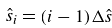 $\hat{s}_{i}={}(i-1)\Delta \hat{s}$
with spacing
$\hat{s}_{i}={}(i-1)\Delta \hat{s}$
with spacing $\Delta \hat{s}=2\pi /N$
(
$\Delta \hat{s}=2\pi /N$
( $N=256$
) and
$N=256$
) and $i = 1$
–
$i = 1$
– $N$
, and the second-order backward difference is used for time
$N$
, and the second-order backward difference is used for time $\hat{t}_{j}=(j-1)\Delta \hat{t}$
with time step
$\hat{t}_{j}=(j-1)\Delta \hat{t}$
with time step $\Delta \hat{t} = 2.5\times 10^{-3}\hat{t}_{P}$
. These values of
$\Delta \hat{t} = 2.5\times 10^{-3}\hat{t}_{P}$
. These values of $\Delta \hat{s}$
and
$\Delta \hat{s}$
and $\Delta \hat{t}$
are determined from convergence tests:
$\Delta \hat{t}$
are determined from convergence tests:
 \begin{align} \frac {\hat{x}_{i+1}^{j}-\hat{x}_{i}^{j}}{\Delta \hat{s}}& = \cos {\psi _{i+1/2}^{j}}, \end{align}
 \begin{align} \frac {\hat{y}_{i+1}^{j}-\hat{y}_{i}^{j}}{\Delta \hat{s}}& = \sin {\psi _{i+1/2}^{j}}, \end{align}
 \begin{align} \frac {\hat{F}_{x,i+1}^{j}-\hat{F}_{x,i}^{j}}{\Delta \hat{s}}- \hat{p}_{i+1/2}^{j}\sin {\psi _{i+1/2}^{j}}& = W_{i+1/2}^{1/3}\frac {3u_{x,i+1/2}^{j}-4u_{x,i+1/2}^{j-1}+u_{x,i+1/2}^{j-2}}{2\Delta \hat{t}}, \end{align}
 \begin{align} &\frac {\hat{F}_{y,i+1}^{j}-\hat{F}_{y,i}^{j}}{\Delta \hat{s}}+ \hat{p}_{i+1/2}^{j}\cos {\psi _{i+1/2}^{j}} = W_{i+1/2}^{1/3}\frac {3u_{y,i+1/2}^{j}-4u_{y,i+1/2}^{j-1}+u_{y,i+1/2}^{j-2}}{2\Delta \hat{t}}, \end{align}
 \begin{align} &\qquad\qquad\qquad\qquad\qquad\hat{p}_{i}^{j} = \frac {C_D \rho _f D}{4\rho _s w_{uni}}(U_n-v_n)_{i}^{j} \lvert U_n-v_n \rvert _{i}^{j}, \end{align}
 \begin{align} &\qquad\qquad\qquad\qquad(U_n-v_n)_{i}^{j}=\frac {\lvert \boldsymbol{\hat{r}}\rvert ^{j-1}_{i}(\partial \hat{H}/\partial \hat{t})^{j}}{2(\hat{H}^{j}-\hat{h})}\sin (\psi _{i}^{j-1}-\gamma _{1,i}^{j-1}) \notag \\& \qquad\qquad\qquad\qquad \qquad + \left [(u_{x,i}^{j-1})^{2}+(u_{y,i}^{j-1})^{2}\right ]^{1/2}\sin (\psi _{i}^{j-1}-\gamma _{2,i}^{j-1}), \end{align}
 \begin{align}& \qquad\qquad\qquad\qquad\qquad\qquad u_{x,i}^{j} = \frac {3\hat{x}_{i}^{j}-4\hat{x}_{i}^{j-1}+\hat{x}_{i}^{j-2}}{2\Delta \hat{t}}, \end{align}
 \begin{align} &\qquad\qquad\qquad\qquad\qquad\qquad u_{y,i}^{j} = \frac {3\hat{y}_{i}^{j}-4\hat{y}_{i}^{j-1}+\hat{y}_{i}^{j-2}}{2\Delta \hat{t}}, \end{align}
 \begin{align} &\frac {\partial W_{i+1/2}}{\partial \hat{s}}(\hat{\kappa }_{i+1/2}^{j}-\hat{\kappa }_{0,i+1/2}) + W_{i+1/2}\left (\frac {\hat{\kappa }_{i+1}^{j}-\hat{\kappa }_{i}^{j}}{\Delta \hat{s}}-\frac {\partial \hat{\kappa }_{0,i+1/2}}{\partial \hat{s}}\right ) \notag \\ & \qquad\qquad = \hat{F}_{x,i+1/2}^{j}\sin {\psi _{i+1/2}^{j}}-\hat{F}_{y,i+1/2}^{j}\cos {\psi _{i+1/2}^{j}}, \end{align}
 \begin{align}& \qquad\qquad\qquad\qquad \frac {\psi _{i+1}^{j}-\psi _{i}^{j}}{\Delta \hat{s}} = \hat{\kappa }_{i+1/2}^{j}, \end{align}
with $\hat{H}^{j}= (2/D)[H_0+A(1-\cos (2\pi \tau \hat{t}_{j}/T))]$
and
$\hat{H}^{j}= (2/D)[H_0+A(1-\cos (2\pi \tau \hat{t}_{j}/T))]$
and $W_{i}=(w(\hat{s}_{i})/w_{uni})^{3}=[1+\Delta \hat{w}\sin ({n_{0}\hat{s}_{i}})]^{3}$
. The subscript
$W_{i}=(w(\hat{s}_{i})/w_{uni})^{3}=[1+\Delta \hat{w}\sin ({n_{0}\hat{s}_{i}})]^{3}$
. The subscript $i$
and superscript
$i$
and superscript $j$
indicate the
$j$
indicate the $i$
th node and
$i$
th node and $j$
th time step, and the index notation
$j$
th time step, and the index notation $X_{i+1/2}$
denotes
$X_{i+1/2}$
denotes $(X_{i+1}+X_{i})/2$
for all variables. Using the built-in Newton’s solver ‘fsolve’ in MATLAB (The MathWorks, Inc.), the above equations are solved at
$(X_{i+1}+X_{i})/2$
for all variables. Using the built-in Newton’s solver ‘fsolve’ in MATLAB (The MathWorks, Inc.), the above equations are solved at $\hat{t}_{j}$
, given the values at
$\hat{t}_{j}$
, given the values at $\hat{t}_{j-1}$
and
$\hat{t}_{j-1}$
and $\hat{t}_{j-2}$
, based on the nonlinear least-squares algorithm (Li & Coleman Reference Li and Coleman1994; Coleman & Li Reference Coleman and Li1996).
$\hat{t}_{j-2}$
, based on the nonlinear least-squares algorithm (Li & Coleman Reference Li and Coleman1994; Coleman & Li Reference Coleman and Li1996).
The elastic loop is initially stationary, and its shape is described by the dimensionless radius $1-(w_{\mathit{uni}}\Delta \hat{w}/D)\sin ({n_{0}\hat{s}})$
. To impose a perturbation that triggers the buckling instability, a random noise
$1-(w_{\mathit{uni}}\Delta \hat{w}/D)\sin ({n_{0}\hat{s}})$
. To impose a perturbation that triggers the buckling instability, a random noise $\epsilon (\hat{s}) \in [-\Delta \hat{s}^2, \Delta \hat{s}^2]$
is added to the local radius for the initial condition at
$\epsilon (\hat{s}) \in [-\Delta \hat{s}^2, \Delta \hat{s}^2]$
is added to the local radius for the initial condition at $\hat{t} = 0$
:
$\hat{t} = 0$
: $\psi (\hat{s},0)=\hat{s}$
,
$\psi (\hat{s},0)=\hat{s}$
, $\hat{x}(\hat{s},0)=[1-(w_{\mathit{uni}}\Delta \hat{w}/D)\sin ({n_{0}\hat{s}})+\epsilon (\hat{s})]\sin {\hat{s}}$
and
$\hat{x}(\hat{s},0)=[1-(w_{\mathit{uni}}\Delta \hat{w}/D)\sin ({n_{0}\hat{s}})+\epsilon (\hat{s})]\sin {\hat{s}}$
and $\hat{y}(\hat{s},0)=-[1-(w_{\mathit{uni}}\Delta \hat{w}/D)\sin ({n_{0}\hat{s}})+\epsilon (\hat{s})]\cos {\hat{s}}$
. The periodic boundary conditions for the closed loop are given by
$\hat{y}(\hat{s},0)=-[1-(w_{\mathit{uni}}\Delta \hat{w}/D)\sin ({n_{0}\hat{s}})+\epsilon (\hat{s})]\cos {\hat{s}}$
. The periodic boundary conditions for the closed loop are given by
 \begin{align} \psi (2\pi ,\hat{t}) = \psi (0,\hat{t}) + 2\pi , \quad \partial _{\hat{s}}\psi (2\pi ,\hat{t}) = \partial _{\hat{s}}\psi (0,\hat{t}), \end{align}
 \begin{align} \hat{x}(2\pi ,\hat{t}) = \hat{x}(0,\hat{t}), \quad \hat{y}(2\pi ,\hat{t}) = \hat{y}(0,\hat{t}), \end{align}
 \begin{align} \hat{F}_{x}(2\pi ,\hat{t}) = \hat{F}_{x}(0,\hat{t}), \quad \hat{F}_{y}(2\pi ,\hat{t}) = \hat{F}_{y}(0,\hat{t}). \end{align}
For validation, test cases for an elastic loop subjected to a constant pressure acting in the surface normal direction ( $\boldsymbol{n}$
) are solved by setting the dimensionless pressure
$\boldsymbol{n}$
) are solved by setting the dimensionless pressure $\hat{p}$
to a constant value, and using the uniform thickness
$\hat{p}$
to a constant value, and using the uniform thickness $\Delta \hat{w}=0$
(Kodio et al. Reference Kodio, Goriely and Vella2020). In figure 10(
$\Delta \hat{w}=0$
(Kodio et al. Reference Kodio, Goriely and Vella2020). In figure 10( $a$
), wrinkle modes are presented for several values of
$a$
), wrinkle modes are presented for several values of $\hat{p}$
, which are similar to the results in figure 3 of Kodio et al. (Reference Kodio, Goriely and Vella2020). The numerical error is evaluated by considering the inextensibility constraint. The total arc length of the elastic loop at every
$\hat{p}$
, which are similar to the results in figure 3 of Kodio et al. (Reference Kodio, Goriely and Vella2020). The numerical error is evaluated by considering the inextensibility constraint. The total arc length of the elastic loop at every $\hat{t}_{j}$
is calculated as
$\hat{t}_{j}$
is calculated as $L_{j}=\varSigma _{i=1}^{N}[(\hat{x}_{i+1}^{j}-\hat{x}_{i}^{j})^2+(\hat{y}_{i+1}^{j}-\hat{y}_{i}^{j})^2]^{1/2}$
. The relative error is defined as
$L_{j}=\varSigma _{i=1}^{N}[(\hat{x}_{i+1}^{j}-\hat{x}_{i}^{j})^2+(\hat{y}_{i+1}^{j}-\hat{y}_{i}^{j})^2]^{1/2}$
. The relative error is defined as $\mathit{\varGamma }=\lvert L_{j}/(2\pi )-1\rvert$
, and is plotted with respect to
$\mathit{\varGamma }=\lvert L_{j}/(2\pi )-1\rvert$
, and is plotted with respect to $\hat{t}$
in figure 10(
$\hat{t}$
in figure 10( $b$
). Although the relative error at
$b$
). Although the relative error at $\hat{t}=0$
is 1.3 %–1.4 % due to the initial perturbation, the magnitude of the relative error is less than
$\hat{t}=0$
is 1.3 %–1.4 % due to the initial perturbation, the magnitude of the relative error is less than $O(10^{-14})$
from the next time step.
$O(10^{-14})$
from the next time step.
( $a$
) Numerical results of dynamic wrinkling under constant pressure
$a$
) Numerical results of dynamic wrinkling under constant pressure $\hat{p}$
(
$\hat{p}$
( $\Delta \hat{t} =$
(
$\Delta \hat{t} =$
( $4\times 10^{-4}$
s)
$4\times 10^{-4}$
s) $/\tau$
). For each
$/\tau$
). For each $\hat{p}$
, deformed profiles at several instants are superimposed, with the colours representing the time sequence
$\hat{p}$
, deformed profiles at several instants are superimposed, with the colours representing the time sequence $\hat{t}$
. (
$\hat{t}$
. ( $b$
) Relative error
$b$
) Relative error $\mathit{\varGamma }$
with respect to
$\mathit{\varGamma }$
with respect to $\hat{t}$
for each case of
$\hat{t}$
for each case of $\hat{p}$
.
$\hat{p}$
.

3. Results and discussion
3.1. Mode selection of wrinkle
In §§ 3.1 and 3.2, the cases of uniform loop thickness are discussed, and the cases of non-uniform thickness are examined in § 3.3. Transient wrinkle patterns are characterised by their apparent mode number $n$
, which is estimated as the number of crest–trough pairs along the loop at a given time. Under the transient hydrodynamic pressure
$n$
, which is estimated as the number of crest–trough pairs along the loop at a given time. Under the transient hydrodynamic pressure $\bar {p}_{\mathit{und}}$
((2.3) and figure 8
$\bar {p}_{\mathit{und}}$
((2.3) and figure 8 $d$
), the apparent mode number
$d$
), the apparent mode number $n$
increases until its maximum
$n$
increases until its maximum $n_{\mathit{max}}$
is reached near
$n_{\mathit{max}}$
is reached near $t\approx t_N$
(defined as the midpoint of the time interval during which
$t\approx t_N$
(defined as the midpoint of the time interval during which $n_{\mathit{max}}$
appears), and subsequently decreases after the pressure reaches its peak
$n_{\mathit{max}}$
appears), and subsequently decreases after the pressure reaches its peak $\bar {p}_{\mathit{max}}$
, as shown in figure 11(
$\bar {p}_{\mathit{max}}$
, as shown in figure 11( $a$
,
$a$
, $b$
); see supplementary movie 1 available at https://doi.org/10.1017/jfm.2026.11651. In the figure, the apparent mode number
$b$
); see supplementary movie 1 available at https://doi.org/10.1017/jfm.2026.11651. In the figure, the apparent mode number $n$
peaks at
$n$
peaks at $n_{\mathit{max}}=9$
after
$n_{\mathit{max}}=9$
after $t=28$
ms and subsequently cascades to lower values. Higher
$t=28$
ms and subsequently cascades to lower values. Higher $\bar {p}_{\mathit{max}}$
results in higher
$\bar {p}_{\mathit{max}}$
results in higher $n_{\mathit{max}}$
with reduced
$n_{\mathit{max}}$
with reduced $t_{N}$
, and vice versa. A cascade of the apparent mode number occurs as two adjacent crests merge into a single crest, similar to the coarsening of wrinkles observed under pulse loading (Box et al. Reference Box, O’Kiely, Kodio, Inizan, Castrejón-Pita and Vella2019; Wang et al. Reference Wang, Sun, He and Ni2023). However, compared with the wrinkle coarsening reported by Box et al. (Reference Box, O’Kiely, Kodio, Inizan, Castrejón-Pita and Vella2019) where the wavelength scales as
$t_{N}$
, and vice versa. A cascade of the apparent mode number occurs as two adjacent crests merge into a single crest, similar to the coarsening of wrinkles observed under pulse loading (Box et al. Reference Box, O’Kiely, Kodio, Inizan, Castrejón-Pita and Vella2019; Wang et al. Reference Wang, Sun, He and Ni2023). However, compared with the wrinkle coarsening reported by Box et al. (Reference Box, O’Kiely, Kodio, Inizan, Castrejón-Pita and Vella2019) where the wavelength scales as $\lambda \sim t^{2/5}$
, the apparent mode number in our experiment decreases somewhat more rapidly than expected from the scaling
$\lambda \sim t^{2/5}$
, the apparent mode number in our experiment decreases somewhat more rapidly than expected from the scaling $n=\pi D/\lambda \sim t^{-2/5}$
(figure 11
$n=\pi D/\lambda \sim t^{-2/5}$
(figure 11 $b$
). Furthermore, although crest merging can also occur under nearly constant loading (Kodio et al. Reference Kodio, Goriely and Vella2020), pressure attenuation after its peak in the present hydrodynamically coupled system allows the apparent mode number to continue to reduce slowly.
$b$
). Furthermore, although crest merging can also occur under nearly constant loading (Kodio et al. Reference Kodio, Goriely and Vella2020), pressure attenuation after its peak in the present hydrodynamically coupled system allows the apparent mode number to continue to reduce slowly.
( $a$
) Evolution of the elastic loop (
$a$
) Evolution of the elastic loop ( $D=80$
mm) under transient hydrodynamic pressure with
$D=80$
mm) under transient hydrodynamic pressure with $\bar {p}_{\mathit{max}}=1800$
Pa (
$\bar {p}_{\mathit{max}}=1800$
Pa ( $\alpha =0.31$
and
$\alpha =0.31$
and $T=111$
ms). See supplementary movie 1. (
$T=111$
ms). See supplementary movie 1. ( $b$
) Temporal change in apparent mode number
$b$
) Temporal change in apparent mode number $n$
and elastic bending energy
$n$
and elastic bending energy $E_b$
for the condition of (
$E_b$
for the condition of ( $a$
). The peak instants of
$a$
). The peak instants of $n$
and
$n$
and $E_b$
(
$E_b$
( $t_N$
and
$t_N$
and $t_E$
, respectively) are denoted by the dashed lines. (
$t_E$
, respectively) are denoted by the dashed lines. ( $c$
) Normalised peak instants
$c$
) Normalised peak instants $t_{E}/t_{P}$
versus
$t_{E}/t_{P}$
versus $t_{N}/t_{P}$
. The solid line and the dashed line denote
$t_{N}/t_{P}$
. The solid line and the dashed line denote $t_{E}/t_{P}=t_{N}/t_{P}$
and
$t_{E}/t_{P}=t_{N}/t_{P}$
and $t_{N}/t_{P}=1$
, respectively.
$t_{N}/t_{P}=1$
, respectively.

The bending energy of the elastic loop, $E_{b}= ({1}/{2})EI\int _{0}^{\pi D}(\kappa -\kappa _{0})^{2}\,\text{d}s$
(Ye et al. Reference Ye, Wei, Huang and Lu2017), where
$E_{b}= ({1}/{2})EI\int _{0}^{\pi D}(\kappa -\kappa _{0})^{2}\,\text{d}s$
(Ye et al. Reference Ye, Wei, Huang and Lu2017), where $\kappa$
and
$\kappa$
and $\kappa _{0}$
denote the local and initial curvature, respectively, exhibits a temporal trend following that of the mode number
$\kappa _{0}$
denote the local and initial curvature, respectively, exhibits a temporal trend following that of the mode number $n$
, but with a different peak time
$n$
, but with a different peak time $t=t_{E}$
. The sequence of the three peak instants of pressure, apparent mode number and bending energy follows
$t=t_{E}$
. The sequence of the three peak instants of pressure, apparent mode number and bending energy follows $t_{P}\lesssim t_{N}\lesssim t_{E}$
as shown in figure 11(
$t_{P}\lesssim t_{N}\lesssim t_{E}$
as shown in figure 11( $c$
). The difference between
$c$
). The difference between $t_N$
and
$t_N$
and $t_E$
indicates continued storage of the elastic energy even as the wrinkles cascade to lower
$t_E$
indicates continued storage of the elastic energy even as the wrinkles cascade to lower $n$
. After the pressure reaches its peak, the continued growth of unstable modes lower than
$n$
. After the pressure reaches its peak, the continued growth of unstable modes lower than $n_{\mathit{max}}$
appears to overtake that of the mode corresponding to
$n_{\mathit{max}}$
appears to overtake that of the mode corresponding to $n_{\mathit{max}}$
, leading to the decrease in
$n_{\mathit{max}}$
, leading to the decrease in $n$
while
$n$
while $E_{b}$
continues to increase. After
$E_{b}$
continues to increase. After $t=t_{E}$
, the cascade to lower modes proceeds as the elastic energy relaxes.
$t=t_{E}$
, the cascade to lower modes proceeds as the elastic energy relaxes.
The results from the low-order numerical simulation (§ 2.4) that resolves the deformation of the loop are compared with the experimental results. Figure 12( $a$
) shows the deformed profiles of the elastic loop in sequence, which were obtained under identical parameters,
$a$
) shows the deformed profiles of the elastic loop in sequence, which were obtained under identical parameters, $D=60$
mm and
$D=60$
mm and $\bar {p}_{\mathit{max}}=1020$
Pa (
$\bar {p}_{\mathit{max}}=1020$
Pa ( $\alpha =(H_0-h)/A=0.5$
,
$\alpha =(H_0-h)/A=0.5$
, $T=87$
ms), corresponding to a case where strong hydrodynamic pressure deforms the loop notably. Although a discrepancy in the profile of the loop between the experimental and numerical cases becomes greater after the apparent mode number reaches its maximum
$T=87$
ms), corresponding to a case where strong hydrodynamic pressure deforms the loop notably. Although a discrepancy in the profile of the loop between the experimental and numerical cases becomes greater after the apparent mode number reaches its maximum $n_{\mathit{max}}$
, both cases exhibit a similar tendency of transient wrinkle development, as shown in the evolution of the apparent mode number
$n_{\mathit{max}}$
, both cases exhibit a similar tendency of transient wrinkle development, as shown in the evolution of the apparent mode number $n$
(figure 12
$n$
(figure 12 $b$
) and the bending energy of the loop
$b$
) and the bending energy of the loop $E_b$
(figure 12
$E_b$
(figure 12 $c$
). There is also a slight difference in the initial value of
$c$
). There is also a slight difference in the initial value of $n$
; the apparent mode number increases from
$n$
; the apparent mode number increases from $n=2$
due to the minor intrinsic eccentricity of the initial loop geometry in the experiment, whereas it increases from
$n=2$
due to the minor intrinsic eccentricity of the initial loop geometry in the experiment, whereas it increases from $n=0$
in the low-order numerical simulation. Nevertheless, the two cases display comparable values of
$n=0$
in the low-order numerical simulation. Nevertheless, the two cases display comparable values of $n_{\mathit{max}}$
occurring at similar times
$n_{\mathit{max}}$
occurring at similar times $t_N\approx 17$
ms (
$t_N\approx 17$
ms ( $n_{\mathit{max}}=7$
for the experiment and
$n_{\mathit{max}}=7$
for the experiment and $n_{\mathit{max}}=8$
for the numerical simulation). In addition, the bending energy
$n_{\mathit{max}}=8$
for the numerical simulation). In addition, the bending energy $E_b$
increases and subsequently decreases in both cases, with peaks occurring at similar times
$E_b$
increases and subsequently decreases in both cases, with peaks occurring at similar times $t_E$
(
$t_E$
( $t_E=28$
ms for the experiment and
$t_E=28$
ms for the experiment and $t_E=23$
ms for the numerical simulation).
$t_E=23$
ms for the numerical simulation).
( $a$
) Comparison of time-evolving wrinkle profiles between experimental (first row) and numerical (second row) results. The parametric conditions for both cases are
$a$
) Comparison of time-evolving wrinkle profiles between experimental (first row) and numerical (second row) results. The parametric conditions for both cases are $D=60$
mm and
$D=60$
mm and $\bar {p}_{\mathit{max}}=1020$
Pa (
$\bar {p}_{\mathit{max}}=1020$
Pa ( $\alpha =0.5$
,
$\alpha =0.5$
, $T=87$
ms). The third and fourth columns correspond to
$T=87$
ms). The third and fourth columns correspond to $t=t_N$
and
$t=t_N$
and $t=t_E$
, respectively. For the numerical results, a crest (blue marker) and a trough (red marker) are highlighted on the deforming loop. Time histories of (
$t=t_E$
, respectively. For the numerical results, a crest (blue marker) and a trough (red marker) are highlighted on the deforming loop. Time histories of ( $b$
) apparent mode number
$b$
) apparent mode number $n$
and (
$n$
and ( $c$
) bending energy
$c$
) bending energy $E_b$
obtained from the experimental (solid line) and numerical (dashed line) results. (
$E_b$
obtained from the experimental (solid line) and numerical (dashed line) results. ( $d$
) Time histories of hydrodynamic pressure
$d$
) Time histories of hydrodynamic pressure $\bar {p}$
at the crest (blue) and trough (red) shown in (
$\bar {p}$
at the crest (blue) and trough (red) shown in ( $a$
). The profile of the undisturbed axisymmetric pressure
$a$
). The profile of the undisturbed axisymmetric pressure $\bar {p}_{\mathit{und}}$
is shown by the black curve for comparison.
$\bar {p}_{\mathit{und}}$
is shown by the black curve for comparison.

To elucidate the effect of fluid–structure interaction arising from loop deformation on the wrinkling behaviour, the temporal evolution of the net hydrodynamic pressure $\bar {p}$
defined in (2.5a
) is examined at a crest (blue marker) and a trough (red marker) depicted in figure 12(
$\bar {p}$
defined in (2.5a
) is examined at a crest (blue marker) and a trough (red marker) depicted in figure 12( $a$
), using the numerical result. Fluid–structure interaction during wrinkling induces spatial non-uniformity in
$a$
), using the numerical result. Fluid–structure interaction during wrinkling induces spatial non-uniformity in $\bar {p}$
(figure 12
$\bar {p}$
(figure 12 $d$
), particularly after the pressure peak of the undisturbed axisymmetric pressure
$d$
), particularly after the pressure peak of the undisturbed axisymmetric pressure $\bar {p}_{\mathit{und}}$
. As the loop deforms, the pressure increases relatively at the bulging crest and decreases at the receding trough (blue and red solid lines in figure 12
$\bar {p}_{\mathit{und}}$
. As the loop deforms, the pressure increases relatively at the bulging crest and decreases at the receding trough (blue and red solid lines in figure 12 $d$
, respectively). However, due to the elastic constraint originating from the closed geometry of the loop, the majority of the loop (except the crest) tends to recede in the radial direction during the deformation and thus experiences the decrease in
$d$
, respectively). However, due to the elastic constraint originating from the closed geometry of the loop, the majority of the loop (except the crest) tends to recede in the radial direction during the deformation and thus experiences the decrease in $\bar {p}$
. In addition, the change in the surface normal
$\bar {p}$
. In addition, the change in the surface normal $\boldsymbol{n}$
between the crest and the trough causes the direction of
$\boldsymbol{n}$
between the crest and the trough causes the direction of $\bar {p}$
to misalign with the radial direction:
$\bar {p}$
to misalign with the radial direction: $\boldsymbol{n}\neq -\hat{\boldsymbol{r}}$
. This spatial non-uniformity in pressure tends to decelerate wrinkle development, ultimately leading to attenuation of the wrinkle profile after reaching its maximum deformation (
$\boldsymbol{n}\neq -\hat{\boldsymbol{r}}$
. This spatial non-uniformity in pressure tends to decelerate wrinkle development, ultimately leading to attenuation of the wrinkle profile after reaching its maximum deformation ( $t\gt t_E$
).
$t\gt t_E$
).
Next, the mode selection of transient wrinkle patterns is discussed, particularly in terms of the maximum mode number $n_{\mathit{max}}$
. Although the time scale required for the development of the maximum mode number is slightly longer than the time required to reach the pressure peak (
$n_{\mathit{max}}$
. Although the time scale required for the development of the maximum mode number is slightly longer than the time required to reach the pressure peak ( $t_P\lesssim t_N$
), the wrinkle corresponding to
$t_P\lesssim t_N$
), the wrinkle corresponding to $n_{\mathit{max}}$
begins to emerge before
$n_{\mathit{max}}$
begins to emerge before $t=t_N$
(at
$t=t_N$
(at $t=19$
ms in figure 11
a,b). This observation suggests that the time scale governing mode selection is shorter than
$t=19$
ms in figure 11
a,b). This observation suggests that the time scale governing mode selection is shorter than $t_N$
, and
$t_N$
, and $t_P$
may therefore be regarded as a natural candidate for characterising this time scale. In figure 12(
$t_P$
may therefore be regarded as a natural candidate for characterising this time scale. In figure 12( $d$
), the spatial non-uniformity of the pressure remains small before the pressure reaches its peak. Consequently, within the time scale relevant to mode selection, the hydrodynamic pressure can be approximated to be spatially uniform (i.e.
$d$
), the spatial non-uniformity of the pressure remains small before the pressure reaches its peak. Consequently, within the time scale relevant to mode selection, the hydrodynamic pressure can be approximated to be spatially uniform (i.e. $\bar {p}\approx \bar {p}_{\mathit{und}}$
for
$\bar {p}\approx \bar {p}_{\mathit{und}}$
for $t\lt t_P$
), and the transient profile of
$t\lt t_P$
), and the transient profile of $\bar {p}_{\mathit{und}}$
can be used to describe the mode-selection mechanism. Accordingly, the magnitude and instant of pressure peak,
$\bar {p}_{\mathit{und}}$
can be used to describe the mode-selection mechanism. Accordingly, the magnitude and instant of pressure peak, $\bar {p}_{\mathit{max}}$
and
$\bar {p}_{\mathit{max}}$
and $t_P$
in (2.4) and figure 8(
$t_P$
in (2.4) and figure 8( $d$
), which are derived from the profile of
$d$
), which are derived from the profile of $\bar {p}_{\mathit{und}}$
, can be chosen as the primary parameters of characterising the increasing pressure during
$\bar {p}_{\mathit{und}}$
, can be chosen as the primary parameters of characterising the increasing pressure during $t\lt t_P$
and the mode selection.
$t\lt t_P$
and the mode selection.
Substituting $T=2\pi t_P/\tan ^{-1}[\alpha ^{1/2}(\alpha +2)^{1/2}]$
from (2.4b
) into (2.4a
), the dimensionless peak pressure
$T=2\pi t_P/\tan ^{-1}[\alpha ^{1/2}(\alpha +2)^{1/2}]$
from (2.4b
) into (2.4a
), the dimensionless peak pressure $\hat{p}_{\mathit{max}}\ (=\bar {p}_{\mathit{max}}hD^3/8EI)$
can be expressed in terms of
$\hat{p}_{\mathit{max}}\ (=\bar {p}_{\mathit{max}}hD^3/8EI)$
can be expressed in terms of $\hat{t}_P\ (=t_P/\tau )$
and
$\hat{t}_P\ (=t_P/\tau )$
and $\alpha$
:
$\alpha$
:
 \begin{equation} \hat{p}_{\mathit{max}}=\frac {C_D\rho _fD}{16\rho _sw}\left [\frac {\tan ^{-1}(\alpha ^{1/2}(\alpha +2)^{1/2})}{\alpha ^{1/2}(\alpha +2)^{1/2}}\right ]^2\hat{t}_{P}^{-2}. \end{equation}
Figure 13( $a$
) shows a correlation between
$a$
) shows a correlation between $\hat{p}_{\mathit{max}}$
and
$\hat{p}_{\mathit{max}}$
and $\hat{t}_{P}$
, indicating that a hydrodynamic pressure profile with lower
$\hat{t}_{P}$
, indicating that a hydrodynamic pressure profile with lower $\hat{t}_P$
has greater
$\hat{t}_P$
has greater $\hat{p}_{\mathit{max}}$
and vice versa. As
$\hat{p}_{\mathit{max}}$
and vice versa. As $\hat{p}_{\mathit{max}}$
increases (or
$\hat{p}_{\mathit{max}}$
increases (or $\hat{t}_{P}$
decreases), the maximum mode number
$\hat{t}_{P}$
decreases), the maximum mode number $n_{\mathit{max}}$
increases correspondingly, revealing
$n_{\mathit{max}}$
increases correspondingly, revealing $\hat{p}_{\mathit{max}}$
as a key dynamic variable that determines
$\hat{p}_{\mathit{max}}$
as a key dynamic variable that determines $n_{\mathit{max}}$
.
$n_{\mathit{max}}$
.
( $a$
) Correlation between maximum pressure
$a$
) Correlation between maximum pressure $\hat{p}_{\mathit{max}}$
and the instant of pressure peak
$\hat{p}_{\mathit{max}}$
and the instant of pressure peak $\hat{t}_{P}$
. The colourbar denotes the maximum apparent mode number
$\hat{t}_{P}$
. The colourbar denotes the maximum apparent mode number $n_{\mathit{max}}$
from experiments. The inset shows the temporal profile of pressure
$n_{\mathit{max}}$
from experiments. The inset shows the temporal profile of pressure $\hat{p}_{\mathit{und}}$
. (
$\hat{p}_{\mathit{und}}$
. ( $b$
) Maximum apparent mode number
$b$
) Maximum apparent mode number $n_{\mathit{max}}$
with respect to maximum pressure
$n_{\mathit{max}}$
with respect to maximum pressure $\hat{p}_{\mathit{max}}$
. The mode selection relation (3.4) is denoted by the black solid line and compared with experimental (grey circles) and low-order numerical (red squares) results.
$\hat{p}_{\mathit{max}}$
. The mode selection relation (3.4) is denoted by the black solid line and compared with experimental (grey circles) and low-order numerical (red squares) results.

To quantitatively explain the dependence of $n_{\mathit{max}}$
on
$n_{\mathit{max}}$
on $\hat{p}_{\mathit{max}}$
, we next present a theoretical analysis based on an energy balance. The profiles of the buckled loop are composed of harmonic modes
$\hat{p}_{\mathit{max}}$
, we next present a theoretical analysis based on an energy balance. The profiles of the buckled loop are composed of harmonic modes $r^{*}(\theta ,t)=\lvert \boldsymbol{r}\rvert =\varSigma _{m=0}^{\infty }a_{m}(t)\cos (m\theta +\varphi _{m})$
. Among harmonic modes, the wrinkle profile eventually conforms to a fastest-growing unstable mode. Modelling the simultaneous growth of all harmonic modes introduces significant nonlinear complexity. As a modelling strategy to avoid dealing with such nonlinearity, we instead consider multiple hypothetical scenarios, each of which involves only a single harmonic mode. The scenario associated with the highest growth rate corresponds to the dominant mode and ultimately represents the behaviour that occurs in reality.
$r^{*}(\theta ,t)=\lvert \boldsymbol{r}\rvert =\varSigma _{m=0}^{\infty }a_{m}(t)\cos (m\theta +\varphi _{m})$
. Among harmonic modes, the wrinkle profile eventually conforms to a fastest-growing unstable mode. Modelling the simultaneous growth of all harmonic modes introduces significant nonlinear complexity. As a modelling strategy to avoid dealing with such nonlinearity, we instead consider multiple hypothetical scenarios, each of which involves only a single harmonic mode. The scenario associated with the highest growth rate corresponds to the dominant mode and ultimately represents the behaviour that occurs in reality.
A wrinkle profile that has a single harmonic mode of a mode number $m$
is given as
$m$
is given as $r^{*}_{m}(\theta ,t)=a_{0}(t)+a_{m}(t)\cos (m\theta )$
; the inextensibility of the elastic loop constrains
$r^{*}_{m}(\theta ,t)=a_{0}(t)+a_{m}(t)\cos (m\theta )$
; the inextensibility of the elastic loop constrains $a_{0}\approx D/2-(m^2+1)a_{m}^2/2D$
. The length scale of deformation is small (
$a_{0}\approx D/2-(m^2+1)a_{m}^2/2D$
. The length scale of deformation is small ( $2a_{m}/D\leqslant O(10^{-1})$
), so an approximate differential arc length of
$2a_{m}/D\leqslant O(10^{-1})$
), so an approximate differential arc length of $r^{*}_{m}\text{d}\theta$
is used to calculate the bending energy
$r^{*}_{m}\text{d}\theta$
is used to calculate the bending energy $E_{b}$
and kinetic energy
$E_{b}$
and kinetic energy $E_{k}$
of the loop, and the work
$E_{k}$
of the loop, and the work $W$
done on the loop by the pressure
$W$
done on the loop by the pressure $\bar {p}_{\mathit{und}}$
. Then,
$\bar {p}_{\mathit{und}}$
. Then, $E_{b}\approx ({1}/{2})EI\int _{0}^{2\pi }(\kappa -\kappa _{0})^{2}r^{*}_{m}\,\text{d}\theta$
and
$E_{b}\approx ({1}/{2})EI\int _{0}^{2\pi }(\kappa -\kappa _{0})^{2}r^{*}_{m}\,\text{d}\theta$
and $E_{k}\approx ({1}/{2})\rho _{s}wh\int _{0}^{2\pi }(\partial _{t}r^{*}_{m})^{2}r^{*}_{m}\,\text{d}\theta$
. The harmonic profile of the wrinkle mode leads to
$E_{k}\approx ({1}/{2})\rho _{s}wh\int _{0}^{2\pi }(\partial _{t}r^{*}_{m})^{2}r^{*}_{m}\,\text{d}\theta$
. The harmonic profile of the wrinkle mode leads to $\kappa \approx \kappa _{0}+\Delta \kappa \cos (m\theta )$
, where
$\kappa \approx \kappa _{0}+\Delta \kappa \cos (m\theta )$
, where $\Delta \kappa =4(m^2-1)a_{m}/D^2$
. The above integrals then yield
$\Delta \kappa =4(m^2-1)a_{m}/D^2$
. The above integrals then yield $E_{b}\approx ({\pi }/{2})EIa_{0}\Delta \kappa ^2$
and
$E_{b}\approx ({\pi }/{2})EIa_{0}\Delta \kappa ^2$
and $E_{k}\approx ({\pi }/{2})\rho _{s}wha_{0}\dot{a}_{m}^2$
. The work done on a unit surface area is
$E_{k}\approx ({\pi }/{2})\rho _{s}wha_{0}\dot{a}_{m}^2$
. The work done on a unit surface area is $\delta W=-\int _{0}^{t}\bar {p}_{\mathit{und}}\partial _{t'}r^{*}_{m}\text{d}t'$
, and thus
$\delta W=-\int _{0}^{t}\bar {p}_{\mathit{und}}\partial _{t'}r^{*}_{m}\text{d}t'$
, and thus $W\approx \int _{0}^{2\pi }\delta Whr^{*}_{m}\,\text{d}\theta =\pi h\int _{0}^{t}\bar {p}_{\mathit{und}}a_{m}\dot{a}_{m}[m^2-(m^2+1)^2a_{m}^2/D^2 ]\, \text{d}t'$
. Neglecting the high-order term
$W\approx \int _{0}^{2\pi }\delta Whr^{*}_{m}\,\text{d}\theta =\pi h\int _{0}^{t}\bar {p}_{\mathit{und}}a_{m}\dot{a}_{m}[m^2-(m^2+1)^2a_{m}^2/D^2 ]\, \text{d}t'$
. Neglecting the high-order term $(a_{m}/D)^2$
in
$(a_{m}/D)^2$
in $E_{b}$
,
$E_{b}$
, $E_{k}$
and
$E_{k}$
and $W$
, the energy balance (
$W$
, the energy balance ( $W=E_{b}+E_{k}$
) is approximated as
$W=E_{b}+E_{k}$
) is approximated as
 \begin{equation} \pi hm^2\int _{0}^{t}\bar {p}_{\mathit{und}}a_{m}\dot{a}_{m} \text{d}t' \approx \frac {4\pi EI}{D^3}(m^{2}-1)^{2}a_{m}^{2} + \frac {\pi \rho _{s}whD}{4}\dot{a}_{m}^{2}. \end{equation}
As a simplified model of the transient $\bar {p}_{\mathit{und}}$
which increases until
$\bar {p}_{\mathit{und}}$
which increases until $t=t_{P}$
, we substitute a linear profile of
$t=t_{P}$
, we substitute a linear profile of $\hat{p}_{\mathit{und}} \ (=\bar {p}_{\mathit{und}}hD^3/8EI)$
with respect to
$\hat{p}_{\mathit{und}} \ (=\bar {p}_{\mathit{und}}hD^3/8EI)$
with respect to $t$
(
$t$
( $\hat{p}_{\mathit{und}}\approx \hat{p}_{\mathit{max}}t/t_{P}$
for
$\hat{p}_{\mathit{und}}\approx \hat{p}_{\mathit{max}}t/t_{P}$
for $t\leqslant t_{P}$
) in (3.2) (inset of figure 13
$t\leqslant t_{P}$
) in (3.2) (inset of figure 13 $a$
). Assuming the exponential growth of
$a$
). Assuming the exponential growth of $a_{m}\sim \exp (\sigma _{m} t/t_{P})$
, a dispersion relation describing the growth of the instability of each unstable mode at
$a_{m}\sim \exp (\sigma _{m} t/t_{P})$
, a dispersion relation describing the growth of the instability of each unstable mode at $t=t_{P}$
is obtained, such that
$t=t_{P}$
is obtained, such that
 \begin{equation} \sigma _{m}^2 \approx \frac {4Ew^{2}t_{P}^{2}}{3\rho _{s}D^{4}}\left [m^{2}\hat{p}_{\mathit{max}}-(m^{2}-1)^{2}\right ]. \end{equation}
Linearly unstable modes exist for $(\hat{p}_{\mathit{max}}/2+1)[1-(1-4/(\hat{p}_{\mathit{max}}+2)^{2})^{1/2}]\lt m^{2}\lt (\hat{p}_{\mathit{max}}/2+1)[1+(1-4/(\hat{p}_{\mathit{max}}+2)^{2})^{1/2}]$
, and the fastest-growing mode corresponds to the integer that is closest to
$(\hat{p}_{\mathit{max}}/2+1)[1-(1-4/(\hat{p}_{\mathit{max}}+2)^{2})^{1/2}]\lt m^{2}\lt (\hat{p}_{\mathit{max}}/2+1)[1+(1-4/(\hat{p}_{\mathit{max}}+2)^{2})^{1/2}]$
, and the fastest-growing mode corresponds to the integer that is closest to
 \begin{equation} n^{*}\approx \left (\frac {\hat{p}_{\mathit{max}}}{2}\right )^{1/2} \end{equation}
with a maximum growth rate of $\sigma _{\mathit{max}}\approx [\hat{p}_{\mathit{max}}(\hat{p}_{\mathit{max}}/4+1)]^{1/2}t_{P}/\tau$
, where
$\sigma _{\mathit{max}}\approx [\hat{p}_{\mathit{max}}(\hat{p}_{\mathit{max}}/4+1)]^{1/2}t_{P}/\tau$
, where $\tau =(3\rho _{s}D^{4}/4w^{2}E)^{1/2}$
denotes the inertial time scale. Parameters
$\tau =(3\rho _{s}D^{4}/4w^{2}E)^{1/2}$
denotes the inertial time scale. Parameters $\hat{p}_{\mathit{max}}$
and
$\hat{p}_{\mathit{max}}$
and $n^*$
have a square-root relationship, and the growth rate is affected by the loop’s inertia (
$n^*$
have a square-root relationship, and the growth rate is affected by the loop’s inertia ( $\rho _{s}$
) under hydrodynamic loading conditions, which were also reported for dynamic buckling induced by a rapid change in surface tension on an elastic loop in Box et al. (Reference Box, Kodio, O’Kiely, Cantelli, Goriely and Vella2020).
$\rho _{s}$
) under hydrodynamic loading conditions, which were also reported for dynamic buckling induced by a rapid change in surface tension on an elastic loop in Box et al. (Reference Box, Kodio, O’Kiely, Cantelli, Goriely and Vella2020).
The dependence of $n_{\mathit{max}}$
on
$n_{\mathit{max}}$
on $\hat{p}_{\mathit{max}}$
predicted by the theoretically derived relation (3.4) is compared with the experimental and low-order numerical results (figure 13
$\hat{p}_{\mathit{max}}$
predicted by the theoretically derived relation (3.4) is compared with the experimental and low-order numerical results (figure 13 $b$
). The parameter ranges considered are
$b$
). The parameter ranges considered are $D=60$
mm,
$D=60$
mm, $\alpha =0.05$
–
$\alpha =0.05$
– $2$
and
$2$
and $T=11$
–
$T=11$
– $1358$
ms, corresponding to
$1358$
ms, corresponding to $\hat{p}_{\mathit{max}}=10$
–
$\hat{p}_{\mathit{max}}=10$
– $8000$
and
$8000$
and $\hat{t}_{P}=0.023$
–
$\hat{t}_{P}=0.023$
– $0.848$
. As intuitively expected, hydrodynamic pressure profiles with higher
$0.848$
. As intuitively expected, hydrodynamic pressure profiles with higher $\hat{p}_{\mathit{max}}$
(or equivalently shorter
$\hat{p}_{\mathit{max}}$
(or equivalently shorter $\hat{t}_P$
) lead to wrinkle patterns with higher
$\hat{t}_P$
) lead to wrinkle patterns with higher $n_{\mathit{max}}$
. However, (3.4) serves as an upper bound for mode selection, which tends to overestimate
$n_{\mathit{max}}$
. However, (3.4) serves as an upper bound for mode selection, which tends to overestimate $n_{\mathit{max}}$
in comparison with the experimental and numerical values for the cases of high
$n_{\mathit{max}}$
in comparison with the experimental and numerical values for the cases of high $\hat{p}_{\mathit{max}}$
(
$\hat{p}_{\mathit{max}}$
( $\hat{p}_{\mathit{max}}\gt 200$
), rather than indicating a direct correlation between
$\hat{p}_{\mathit{max}}\gt 200$
), rather than indicating a direct correlation between $\hat{p}_{\mathit{max}}$
and
$\hat{p}_{\mathit{max}}$
and $n_{\mathit{max}}$
; specifically,
$n_{\mathit{max}}$
; specifically, $n_{\mathit{max}}\lesssim n^{*}$
.
$n_{\mathit{max}}\lesssim n^{*}$
.
The discrepancy between $n^{*}$
and
$n^{*}$
and $n_{\mathit{max}}$
can be attributed to the simplifying assumptions associated with the undisturbed pressure model
$n_{\mathit{max}}$
can be attributed to the simplifying assumptions associated with the undisturbed pressure model $\hat{p}_{\mathit{und}}$
used in deriving (3.4), which does not account for the influence of fluid–structure interaction on the pressure. As the elastic loop deforms, the net hydrodynamic pressure acting on the loop is locally alleviated through changes in the relative flow velocity (2.5a
) and surface orientation (2.6a
). According to the above linear stability analysis, the growth rate of the fastest-growing mode increases with the mode number as
$\hat{p}_{\mathit{und}}$
used in deriving (3.4), which does not account for the influence of fluid–structure interaction on the pressure. As the elastic loop deforms, the net hydrodynamic pressure acting on the loop is locally alleviated through changes in the relative flow velocity (2.5a
) and surface orientation (2.6a
). According to the above linear stability analysis, the growth rate of the fastest-growing mode increases with the mode number as $\sigma _{\mathit{max}}\approx [n^{*2}(n^{*2}+2)]^{1/2}\hat{t}_P$
from (3.4) and the following expression of
$\sigma _{\mathit{max}}\approx [n^{*2}(n^{*2}+2)]^{1/2}\hat{t}_P$
from (3.4) and the following expression of $\sigma _{\mathit{max}}$
. Since
$\sigma _{\mathit{max}}$
. Since $\partial r^{*}_{n^{*}}/\partial t\propto \dot{a}_{n^{*}}\propto \sigma _{\mathit{max}}$
, the magnitude of the local velocity of the deforming loop (
$\partial r^{*}_{n^{*}}/\partial t\propto \dot{a}_{n^{*}}\propto \sigma _{\mathit{max}}$
, the magnitude of the local velocity of the deforming loop ( $\lvert \partial \boldsymbol{r}/\partial t\rvert$
) also increases with the mode number. This increase in the local loop velocity leads to a reduction in the relative flow velocity (2.5b
) and consequently to an attenuation of the actual hydrodynamic pressure (2.5a
). Moreover, as the number of wrinkle lobes increases, a greater portion of the loop experiences a reduction in the pressure acting towards the normal direction (2.6a
) due to changes in the surface normal
$\lvert \partial \boldsymbol{r}/\partial t\rvert$
) also increases with the mode number. This increase in the local loop velocity leads to a reduction in the relative flow velocity (2.5b
) and consequently to an attenuation of the actual hydrodynamic pressure (2.5a
). Moreover, as the number of wrinkle lobes increases, a greater portion of the loop experiences a reduction in the pressure acting towards the normal direction (2.6a
) due to changes in the surface normal $\boldsymbol{n}$
during buckling. That is, in actual scenarios, the combined effects of pressure attenuation and spatial non-uniformity become more pronounced for the higher mode number. As a result, the linear stability analysis that neglects such combined effects overestimates
$\boldsymbol{n}$
during buckling. That is, in actual scenarios, the combined effects of pressure attenuation and spatial non-uniformity become more pronounced for the higher mode number. As a result, the linear stability analysis that neglects such combined effects overestimates $n_{\mathit{max}}$
, in particular for the cases of high
$n_{\mathit{max}}$
, in particular for the cases of high $\hat{p}_{\mathit{max}}$
.
$\hat{p}_{\mathit{max}}$
.
The value of $n_{\mathit{max}}$
with respect to
$n_{\mathit{max}}$
with respect to $\hat{p}_{\mathit{max}}$
also differs between the experimental and numerical results, and the difference is notable for higher
$\hat{p}_{\mathit{max}}$
also differs between the experimental and numerical results, and the difference is notable for higher $\hat{p}_{\mathit{max}}$
(figure 13
$\hat{p}_{\mathit{max}}$
(figure 13 $b$
). Generally, the numerical results tend to predict higher values of
$b$
). Generally, the numerical results tend to predict higher values of $n_{\mathit{max}}$
than those observed experimentally. Although the elastic loop is assumed to be inextensible in both the numerical model and the linear stability analysis, the circumferential length of the loop undergoing wrinkling actually exhibits a transient change in the experiments. Prior to buckling, the hydrodynamic pressure pushes the initially circular elastic loop radially inwards, inducing a reduction in the circumferential length. For cases with high
$n_{\mathit{max}}$
than those observed experimentally. Although the elastic loop is assumed to be inextensible in both the numerical model and the linear stability analysis, the circumferential length of the loop undergoing wrinkling actually exhibits a transient change in the experiments. Prior to buckling, the hydrodynamic pressure pushes the initially circular elastic loop radially inwards, inducing a reduction in the circumferential length. For cases with high $\hat{p}_{\mathit{max}}$
, this reduction is more distinct than for cases with low
$\hat{p}_{\mathit{max}}$
, this reduction is more distinct than for cases with low $\hat{p}_{\mathit{max}}$
. For example, the average circumferential strain
$\hat{p}_{\mathit{max}}$
. For example, the average circumferential strain $\epsilon =\Delta L/\pi D$
evaluated at the instant of peak pressure,
$\epsilon =\Delta L/\pi D$
evaluated at the instant of peak pressure, $\hat{t}=\hat{t}_{P}$
, is
$\hat{t}=\hat{t}_{P}$
, is $\epsilon =0.048$
for
$\epsilon =0.048$
for $\hat{p}_{\mathit{max}}=3420$
, whereas it is
$\hat{p}_{\mathit{max}}=3420$
, whereas it is $\epsilon =0.006$
for
$\epsilon =0.006$
for $\hat{p}_{\mathit{max}}=136$
. Additional elastic stretch energy
$\hat{p}_{\mathit{max}}=136$
. Additional elastic stretch energy $E_s$
by the circumferential contraction scales with the square of the strain
$E_s$
by the circumferential contraction scales with the square of the strain $\epsilon$
(
$\epsilon$
( $E_s\sim ({1}/{2})E\epsilon ^2 \times \pi Dwh$
). Due to partial conversion into additional stretch energy
$E_s\sim ({1}/{2})E\epsilon ^2 \times \pi Dwh$
). Due to partial conversion into additional stretch energy $E_s$
, a fraction of the hydrodynamic work converted into the bending energy is smaller than that predicted with the assumption of an inextensible loop. This redistribution of energy is expected to bias unstable modes towards lower mode numbers in the experiments. Because the circumferential strain and the elastic strain energy increase with
$E_s$
, a fraction of the hydrodynamic work converted into the bending energy is smaller than that predicted with the assumption of an inextensible loop. This redistribution of energy is expected to bias unstable modes towards lower mode numbers in the experiments. Because the circumferential strain and the elastic strain energy increase with $\hat{p}_{\mathit{max}}$
, greater deviations from inextensibility for the cases of high
$\hat{p}_{\mathit{max}}$
, greater deviations from inextensibility for the cases of high $\hat{p}_{\mathit{max}}$
lead to lower values of the experimental
$\hat{p}_{\mathit{max}}$
lead to lower values of the experimental $n_{\mathit{max}}$
in figure 13(
$n_{\mathit{max}}$
in figure 13( $b$
).
$b$
).
3.2. Mode similarity
( $a$
) Correlation between degree of similarity,
$a$
) Correlation between degree of similarity, $A_{n_{\mathit{max}}}/\lambda _{n_{\mathit{max}}}$
, and relative growth-time of the apparent mode
$A_{n_{\mathit{max}}}/\lambda _{n_{\mathit{max}}}$
, and relative growth-time of the apparent mode $n_{\mathit{max}}$
,
$n_{\mathit{max}}$
, $\Delta t_{P/2}/\tau _{N}$
. (
$\Delta t_{P/2}/\tau _{N}$
. ( $b$
) Instantaneous deformation profiles illustrating lower
$b$
) Instantaneous deformation profiles illustrating lower $A_{n_{\mathit{max}}}/\lambda _{n_{\mathit{max}}}$
(left panel) and higher
$A_{n_{\mathit{max}}}/\lambda _{n_{\mathit{max}}}$
(left panel) and higher $A_{n_{\mathit{max}}}/\lambda _{n_{\mathit{max}}}$
(right panel) for each
$A_{n_{\mathit{max}}}/\lambda _{n_{\mathit{max}}}$
(right panel) for each $n_{\mathit{max}}$
. The values of
$n_{\mathit{max}}$
. The values of $A_{n_{\mathit{max}}}/\lambda _{n_{\mathit{max}}}$
(left, right) are (
$A_{n_{\mathit{max}}}/\lambda _{n_{\mathit{max}}}$
(left, right) are ( $0.010$
,
$0.010$
, $0.033$
) for
$0.033$
) for $n_{\mathit{max}} = 4$
, (
$n_{\mathit{max}} = 4$
, ( $0.021$
,
$0.021$
, $0.050$
) for
$0.050$
) for $n_{\mathit{max}} = 5$
and (
$n_{\mathit{max}} = 5$
and ( $0.047$
,
$0.047$
, $0.103$
) for
$0.103$
) for $n_{\mathit{max}} = 6$
.
$n_{\mathit{max}} = 6$
.

When the apparent mode number $n$
reaches its maximum
$n$
reaches its maximum $n_{\mathit{max}}$
as shown in figure 11(
$n_{\mathit{max}}$
as shown in figure 11( $b$
), the regularity of the wrinkle morphology differs by the magnitude of
$b$
), the regularity of the wrinkle morphology differs by the magnitude of $n_{\mathit{max}}$
. For cases with lower
$n_{\mathit{max}}$
. For cases with lower $n_{\mathit{max}}$
,
$n_{\mathit{max}}$
, $t_{N}/t_{P}$
increases (figure 11
$t_{N}/t_{P}$
increases (figure 11 $c$
), indicating that the duration of pressure loading is small compared with the relative time scale of mode growth. The short duration of pressure loading restricts the growth of lower
$c$
), indicating that the duration of pressure loading is small compared with the relative time scale of mode growth. The short duration of pressure loading restricts the growth of lower $n_{\mathit{max}}$
and produces a less-distinct crest–trough pattern than that of higher
$n_{\mathit{max}}$
and produces a less-distinct crest–trough pattern than that of higher $n_{\mathit{max}}$
. Therefore, the physical condition under which a distinct crest–trough pattern forms needs to be elucidated.
$n_{\mathit{max}}$
. Therefore, the physical condition under which a distinct crest–trough pattern forms needs to be elucidated.
Although the hydrodynamic pressure varies spatiotemporally, the spatial non-uniformity induced by fluid–structure interaction remains limited when loop deformation is weak. Under such a condition, the transient characteristics of the undisturbed axisymmetric hydrodynamic pressure $\hat{p}_{\mathit{und}}$
are useful to describe the factors influencing the regularity of wrinkle morphology. Accordingly, we focus on the transient profile of
$\hat{p}_{\mathit{und}}$
are useful to describe the factors influencing the regularity of wrinkle morphology. Accordingly, we focus on the transient profile of $\hat{p}_{\mathit{und}}$
to explain the emergence of regular wrinkle patterns. It is plausible to presume that the time scale for the growth of unstable harmonic modes under the transient
$\hat{p}_{\mathit{und}}$
to explain the emergence of regular wrinkle patterns. It is plausible to presume that the time scale for the growth of unstable harmonic modes under the transient $\hat{p}_{\mathit{und}}$
is analogous to that under a piecewise-constant
$\hat{p}_{\mathit{und}}$
is analogous to that under a piecewise-constant $\hat{p}_{\mathit{und}}$
(
$\hat{p}_{\mathit{und}}$
( $\hat{p}_{\mathit{und}}=0$
for
$\hat{p}_{\mathit{und}}=0$
for $t\lt 0$
and
$t\lt 0$
and $\hat{p}_{\mathit{und}}=\hat{p}_{\mathit{max}}$
for
$\hat{p}_{\mathit{und}}=\hat{p}_{\mathit{max}}$
for $t\geqslant 0$
), considering that the pressure increases rapidly from the threshold pressure of each unstable mode to
$t\geqslant 0$
), considering that the pressure increases rapidly from the threshold pressure of each unstable mode to $\hat{p}_{\mathit{max}}$
in our study. The fastest-growing mode under a constant
$\hat{p}_{\mathit{max}}$
in our study. The fastest-growing mode under a constant $\hat{p}_{\mathit{und}} = \hat{p}_{\mathit{max}}$
(
$\hat{p}_{\mathit{und}} = \hat{p}_{\mathit{max}}$
( $t\geqslant 0$
) has a wavenumber of
$t\geqslant 0$
) has a wavenumber of $k=(2\hat{p}_{\mathit{max}})^{1/2}/D$
and a growth rate of
$k=(2\hat{p}_{\mathit{max}})^{1/2}/D$
and a growth rate of $\sigma =(2\hat{p}_{\mathit{max}}/hD^{2})(EI/\rho _{s})^{1/2}$
(Box et al. Reference Box, Kodio, O’Kiely, Cantelli, Goriely and Vella2020; Kodio et al. Reference Kodio, Goriely and Vella2020). The reciprocal of
$\sigma =(2\hat{p}_{\mathit{max}}/hD^{2})(EI/\rho _{s})^{1/2}$
(Box et al. Reference Box, Kodio, O’Kiely, Cantelli, Goriely and Vella2020; Kodio et al. Reference Kodio, Goriely and Vella2020). The reciprocal of $\sigma$
represents the time scale for the growth of the fastest-growing mode, and is denoted as
$\sigma$
represents the time scale for the growth of the fastest-growing mode, and is denoted as $\tau _{N}=(hD^{2}/2\hat{p}_{\mathit{max}})(\rho _{s}/EI)^{1/2}$
. Considering that
$\tau _{N}=(hD^{2}/2\hat{p}_{\mathit{max}})(\rho _{s}/EI)^{1/2}$
. Considering that $\Delta t_{P/2}$
given in (2.4c
) and figure 8(
$\Delta t_{P/2}$
given in (2.4c
) and figure 8( $d$
) represents the duration of dimensionless pressure greater than
$d$
) represents the duration of dimensionless pressure greater than $\hat{p}_{\mathit{max}}/2$
, the relative growth-time of the apparent mode
$\hat{p}_{\mathit{max}}/2$
, the relative growth-time of the apparent mode $n_{\mathit{max}}$
can be defined as
$n_{\mathit{max}}$
can be defined as $\Delta t_{P/2}/\tau _{N} \ (\propto \bar {p}_{\mathit{max}}\Delta t_{P/2})$
, and it indicates how long significant hydrodynamic pressure (exceeding
$\Delta t_{P/2}/\tau _{N} \ (\propto \bar {p}_{\mathit{max}}\Delta t_{P/2})$
, and it indicates how long significant hydrodynamic pressure (exceeding $\hat{p}_{\mathit{max}}/2$
) is exerted, compared with the time scale required for the apparent mode
$\hat{p}_{\mathit{max}}/2$
) is exerted, compared with the time scale required for the apparent mode $n_{\mathit{max}}$
to develop.
$n_{\mathit{max}}$
to develop.
To evaluate how regularly a wrinkle pattern is formed for low $n_{\mathit{max}}$
, we quantify its degree of similarity to a pure harmonic mode and compare this measure with respect to
$n_{\mathit{max}}$
, we quantify its degree of similarity to a pure harmonic mode and compare this measure with respect to $\Delta t_{P/2}/\tau _{N}$
. The amplitudes of the harmonic modes are determined via modal decomposition of the shape profile
$\Delta t_{P/2}/\tau _{N}$
. The amplitudes of the harmonic modes are determined via modal decomposition of the shape profile $r^{*}(\theta ,t)=\varSigma _{m=0}^{\infty }a_{m}(t)\cos (m\theta +\varphi _{m})$
, and the maximum amplitude of the mode
$r^{*}(\theta ,t)=\varSigma _{m=0}^{\infty }a_{m}(t)\cos (m\theta +\varphi _{m})$
, and the maximum amplitude of the mode $m = n_{\mathit{max}}$
is
$m = n_{\mathit{max}}$
is $A_{n_{\mathit{max}}}=\mathrm{max}[a_{n_{\mathit{max}}}(t)]$
. Then
$A_{n_{\mathit{max}}}=\mathrm{max}[a_{n_{\mathit{max}}}(t)]$
. Then $A_{n_{\mathit{max}}}$
is normalised by the characteristic wavelength of a pure harmonic mode,
$A_{n_{\mathit{max}}}$
is normalised by the characteristic wavelength of a pure harmonic mode, $\lambda _{n_{\mathit{max}}}=\pi D/n_{\mathit{max}}$
.
$\lambda _{n_{\mathit{max}}}=\pi D/n_{\mathit{max}}$
.
As the degree of similarity, $A_{n_{\mathit{max}}}/\lambda _{n_{\mathit{max}}}$
, increases, the wrinkle patterns for
$A_{n_{\mathit{max}}}/\lambda _{n_{\mathit{max}}}$
, increases, the wrinkle patterns for $n_{\mathit{max}}=4,\ 5$
and
$n_{\mathit{max}}=4,\ 5$
and $6$
(which represent the group of low
$6$
(which represent the group of low $n_{\mathit{max}}$
) increasingly resemble a pure harmonic mode, and the trend of
$n_{\mathit{max}}$
) increasingly resemble a pure harmonic mode, and the trend of $A_{n_{\mathit{max}}}/\lambda _{n_{\mathit{max}}}$
is positively correlated with
$A_{n_{\mathit{max}}}/\lambda _{n_{\mathit{max}}}$
is positively correlated with $\Delta t_{P/2}/\tau _{N}$
, as shown in figure 14(
$\Delta t_{P/2}/\tau _{N}$
, as shown in figure 14( $a$
). These results indicate that
$a$
). These results indicate that $\Delta t_{P/2}/\tau _{N}$
is crucial for the emergence of a distinct wrinkle pattern that is closer to the pure harmonic mode with
$\Delta t_{P/2}/\tau _{N}$
is crucial for the emergence of a distinct wrinkle pattern that is closer to the pure harmonic mode with $n_{\mathit{max}}$
; even with the same
$n_{\mathit{max}}$
; even with the same $n_{\mathit{max}}$
, mode similarity can differ by input conditions as depicted in figure 14(
$n_{\mathit{max}}$
, mode similarity can differ by input conditions as depicted in figure 14( $b$
). Furthermore, as
$b$
). Furthermore, as $n_{\mathit{max}}$
decreases, the upper limit of
$n_{\mathit{max}}$
decreases, the upper limit of $\Delta t_{P/2}/\tau _{N}$
decreases accordingly due to the increase in
$\Delta t_{P/2}/\tau _{N}$
decreases accordingly due to the increase in $\tau _{N}$
, which in turn limits
$\tau _{N}$
, which in turn limits $A_{n_{\mathit{max}}}/\lambda _{n_{\mathit{max}}}$
to lower values (figure 14
$A_{n_{\mathit{max}}}/\lambda _{n_{\mathit{max}}}$
to lower values (figure 14 $a$
). Consequently, distinct wrinkle patterns are difficult to observe for the case of very low
$a$
). Consequently, distinct wrinkle patterns are difficult to observe for the case of very low $n_{\mathit{max}}$
(e.g.
$n_{\mathit{max}}$
(e.g. $n_{\mathit{max}}=3$
).
$n_{\mathit{max}}=3$
).
( $a$
) Sequential change of wrinkle pattern with non-uniform loop thickness
$a$
) Sequential change of wrinkle pattern with non-uniform loop thickness $w$
(
$w$
( $n_{0}=3$
);
$n_{0}=3$
); $D=50$
mm,
$D=50$
mm, $w_{\mathit{uni}}=1.3$
mm,
$w_{\mathit{uni}}=1.3$
mm, $\Delta \hat{w}=0.21$
,
$\Delta \hat{w}=0.21$
, $\hat{p}_{\mathit{max}}=110$
(
$\hat{p}_{\mathit{max}}=110$
( $\alpha =0.2$
,
$\alpha =0.2$
, $T=107$
ms). Deformation profiles from experimental (top, black) and numerical (bottom, red) results are compared; see supplementary movie 2. (
$T=107$
ms). Deformation profiles from experimental (top, black) and numerical (bottom, red) results are compared; see supplementary movie 2. ( $b$
) Degree of mode similarity,
$b$
) Degree of mode similarity, $A_{n_{\mathit{max}}}/\lambda _{n_{\mathit{max}}}$
, with respect to amplitude of loop thickness
$A_{n_{\mathit{max}}}/\lambda _{n_{\mathit{max}}}$
, with respect to amplitude of loop thickness $\Delta \hat{w}$
(
$\Delta \hat{w}$
( $n_{0}=3$
);
$n_{0}=3$
); $D=60$
mm and
$D=60$
mm and $w_{\mathit{uni}}=1.2$
mm. Values of
$w_{\mathit{uni}}=1.2$
mm. Values of $\hat{p}_{\mathit{max}}$
differ by symbol colour, whereas
$\hat{p}_{\mathit{max}}$
differ by symbol colour, whereas $\alpha$
is fixed to
$\alpha$
is fixed to $\alpha =0.5$
. The inset shows
$\alpha =0.5$
. The inset shows $\Delta \hat{\kappa }_{0}$
versus
$\Delta \hat{\kappa }_{0}$
versus $\Delta \hat{w}$
.
$\Delta \hat{w}$
.

3.3. Effects of non-uniform thickness
In contrast to the cases of uniform loop thickness, buckling instability in a specific mode (even with very low $n_{\mathit{max}}$
) can be more easily triggered in an elastic loop with non-uniform
$n_{\mathit{max}}$
) can be more easily triggered in an elastic loop with non-uniform $w(s)$
, where
$w(s)$
, where $s$
is the curvilinear coordinate in figure 9(
$s$
is the curvilinear coordinate in figure 9( $a$
). For example, by varying the thickness profile as
$a$
). For example, by varying the thickness profile as $w(s)=w_{\mathit{uni}}[1+\Delta \hat{w}\sin (2n_{0}s/D)]$
(i.e. the initial centreline of the loop’s cross-section as
$w(s)=w_{\mathit{uni}}[1+\Delta \hat{w}\sin (2n_{0}s/D)]$
(i.e. the initial centreline of the loop’s cross-section as $\lvert \boldsymbol{r}_{0}\rvert =D/2-(w_{\mathit{uni}}\Delta \hat{w}/2)\sin (2n_{0}s/D)$
), a wrinkle pattern with a constant mode number
$\lvert \boldsymbol{r}_{0}\rvert =D/2-(w_{\mathit{uni}}\Delta \hat{w}/2)\sin (2n_{0}s/D)$
), a wrinkle pattern with a constant mode number $n_0$
is produced clearly over the entire pressure loading period in both the experiment and the numerical analysis (figure 15
a and supplementary movie 2 for
$n_0$
is produced clearly over the entire pressure loading period in both the experiment and the numerical analysis (figure 15
a and supplementary movie 2 for $n_{0}=3$
). Although the degree of deformation of the elastic loop is larger for the numerical case than that for the experimental case, the local points with the minimum thickness
$n_{0}=3$
). Although the degree of deformation of the elastic loop is larger for the numerical case than that for the experimental case, the local points with the minimum thickness $w=w_{\mathit{uni}}(1-\Delta \hat{w})$
on the loop buckle to form the crests of the wrinkle pattern consistently for both cases. Such distinct wrinkle patterns with a very low mode number are challenging to produce for the cases of uniform loop thickness.
$w=w_{\mathit{uni}}(1-\Delta \hat{w})$
on the loop buckle to form the crests of the wrinkle pattern consistently for both cases. Such distinct wrinkle patterns with a very low mode number are challenging to produce for the cases of uniform loop thickness.
The non-uniformity of the loop thickness results in inhomogeneous bending resistance and non-uniform initial curvature $\kappa _{0}(s)$
(figure 9
$\kappa _{0}(s)$
(figure 9 $b$
). The variation in
$b$
). The variation in $\kappa _{0}(s)$
along the loop, which is quantified as
$\kappa _{0}(s)$
along the loop, which is quantified as $\Delta \hat{\kappa }_{0}=(D/2)(\mathrm{max}[\kappa _{0}(s)]-\mathrm{min}[\kappa _{0}(s)])$
, increases linearly with
$\Delta \hat{\kappa }_{0}=(D/2)(\mathrm{max}[\kappa _{0}(s)]-\mathrm{min}[\kappa _{0}(s)])$
, increases linearly with $\Delta \hat{w}$
(inset of figure 15
$\Delta \hat{w}$
(inset of figure 15 $b$
). A non-zero value of
$b$
). A non-zero value of $\Delta \hat{w}$
produces wrinkle patterns of a specific mode (
$\Delta \hat{w}$
produces wrinkle patterns of a specific mode ( $n_{0}=3$
) consistently in figure 15(
$n_{0}=3$
) consistently in figure 15( $b$
). Although the trend of the degree of mode similarity
$b$
). Although the trend of the degree of mode similarity $A_{n_{\mathit{max}}}/\lambda _{n_{\mathit{max}}}$
with respect to
$A_{n_{\mathit{max}}}/\lambda _{n_{\mathit{max}}}$
with respect to $\Delta \hat{w}$
differs by
$\Delta \hat{w}$
differs by $\hat{p}_{\mathit{max}}$
,
$\hat{p}_{\mathit{max}}$
, $A_{n_{\mathit{max}}}/\lambda _{n_{\mathit{max}}}$
generally tends to increase with
$A_{n_{\mathit{max}}}/\lambda _{n_{\mathit{max}}}$
generally tends to increase with $\Delta \hat{w}$
in most cases, which is particularly pronounced for high
$\Delta \hat{w}$
in most cases, which is particularly pronounced for high $\hat{p}_{\mathit{max}}$
. When the effect of non-uniform initial curvature is excluded and only the effect of inhomogeneous bending resistance is considered by setting
$\hat{p}_{\mathit{max}}$
. When the effect of non-uniform initial curvature is excluded and only the effect of inhomogeneous bending resistance is considered by setting $\hat{\kappa }_{0}=1$
and
$\hat{\kappa }_{0}=1$
and $\partial \hat{\kappa }_{0}/\partial \hat{s}=0$
(2.8e
) in the low-order numerical simulation, the elastic loop exhibits a transient wrinkling behaviour similar to that of the elastic loop with uniform thickness in § 3.1. That is, the apparent mode number increases until
$\partial \hat{\kappa }_{0}/\partial \hat{s}=0$
(2.8e
) in the low-order numerical simulation, the elastic loop exhibits a transient wrinkling behaviour similar to that of the elastic loop with uniform thickness in § 3.1. That is, the apparent mode number increases until $n_{\mathit{max}}=7$
and subsequently decreases, rather than exhibiting a specific mode (
$n_{\mathit{max}}=7$
and subsequently decreases, rather than exhibiting a specific mode ( $n_0=3$
) over time although the other conditions except the initial curvature are identical to those of figure 15(
$n_0=3$
) over time although the other conditions except the initial curvature are identical to those of figure 15( $a$
). From these results, we conjecture that the non-uniform initial curvature plays an important role in triggering low-mode regular wrinkling.
$a$
). From these results, we conjecture that the non-uniform initial curvature plays an important role in triggering low-mode regular wrinkling.
4. Concluding remarks
We have investigated the transient wrinkling of a closed elastic loop driven by a well-defined, time-varying hydrodynamic pressure produced in a narrow gap. Under the transient load, the apparent wrinkle mode number $n$
rises rapidly to its maximum
$n$
rises rapidly to its maximum $n_{\mathit{max}}$
near the pressure peak, and subsequently cascades to lower values during the later stage of the response as the pressure attenuates. The elastic bending energy peaks later than the apparent wrinkle mode, indicating continued storage of elastic energy during wrinkle coarsening. An energy-balance model together with a low-order numerical calculation indicates that a dimensionless descriptor of the transient load, its peak magnitude
$n_{\mathit{max}}$
near the pressure peak, and subsequently cascades to lower values during the later stage of the response as the pressure attenuates. The elastic bending energy peaks later than the apparent wrinkle mode, indicating continued storage of elastic energy during wrinkle coarsening. An energy-balance model together with a low-order numerical calculation indicates that a dimensionless descriptor of the transient load, its peak magnitude $\hat{p}_{\mathit{max}}$
, governs mode selection. For the same apparent wrinkle mode, pattern similarity (closeness to a pure harmonic) is determined by the ratio of the loading time to the growth time of the fastest mode. In addition, modest geometric heterogeneity enables more regular wrinkling; spatial variations in the loop thickness bias the onset of buckling towards the thinnest locations of the loop and thus can generate distinct wrinkle patterns of low
$\hat{p}_{\mathit{max}}$
, governs mode selection. For the same apparent wrinkle mode, pattern similarity (closeness to a pure harmonic) is determined by the ratio of the loading time to the growth time of the fastest mode. In addition, modest geometric heterogeneity enables more regular wrinkling; spatial variations in the loop thickness bias the onset of buckling towards the thinnest locations of the loop and thus can generate distinct wrinkle patterns of low $n_{\mathit{max}}$
.
$n_{\mathit{max}}$
.
The present study proposes a practical methodology to attain transient compressive loading using a flow, without embedding actuators in a structure. This approach enables time-resolved mechanical guidance of dynamic buckling states that are otherwise difficult to generate and characterise experimentally. By linking flow kinematics to the resulting pressure profiles, predictive control parameters for wrinkling are derived for an elastic loop. Beyond this specific geometry, our method based on transient elastohydrodynamic instability can provide a broader strategy in soft-matter actuation and adaptive morphing where fluid forces are used to drive deformation.
Supplementary movies
Supplementary movies are available at https://doi.org/10.1017/jfm.2026.11651.
Funding
This work was supported by the National Research Foundation of Korea (NRF) grant funded by the Korea government (MSIT) (RS-2024-00355146) and the InnoCORE programme of the Ministry of Science and ICT (N10260091).
Declaration of interests
The authors report no conflict of interest.
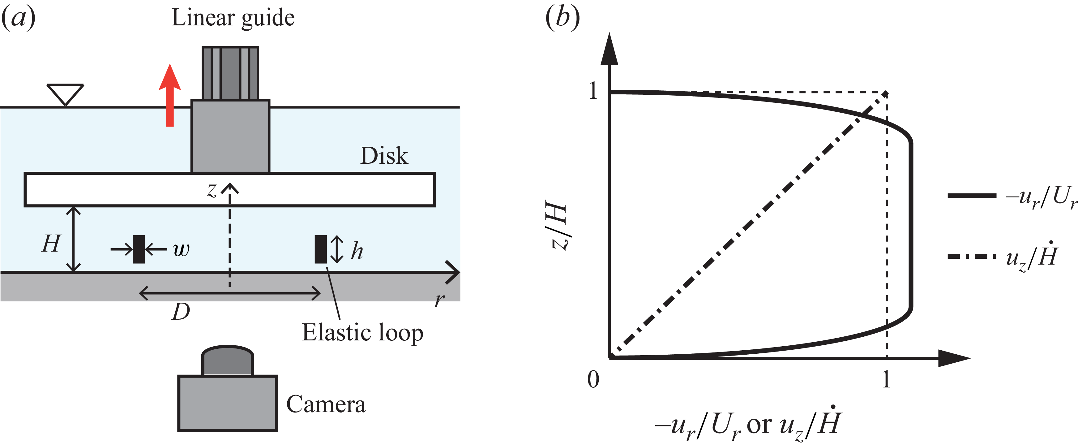
 a
a H(t)
H(t) H0=2.1
 5.0
5.0 A=1.5
A=1.5 3.6
3.6 T=69
T=69 135
135 b
b −ur/Ur
 uz/H˙
uz/H˙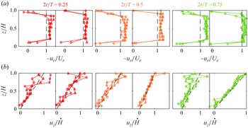
 a
a −ur/Ur
 b
b uz/H˙
uz/H˙ [H0,A,T]
 r=20
r=20
 a
a b
b D
D H0
H0 A
A T
T
 D
D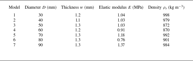
 h=2
h=2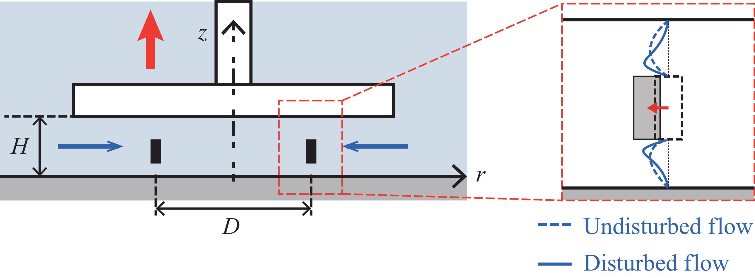

 a
a a
a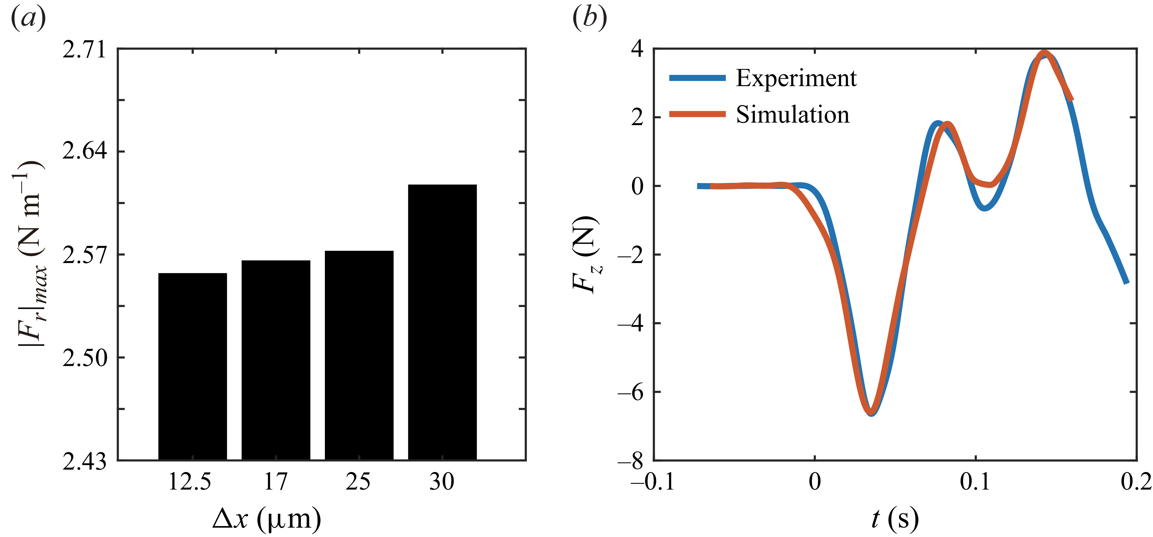
 a
a |Fr|max
 T=0.13
 D=80
D=80 b
b Fz
Fz T=0.33
 a
a t/T=0.16
 D=80
D=80 T=0.13
 D=60
D=60 T=0.14
 b
b p¯und
p¯und p¯und=(1/2)CDρfU2
 D=80
D=80 D=60
D=60 c
c CD
CD T
T b
b d
d p¯und
p¯und H(t)
H(t) H=H0+A[1−cos(2πt/T)]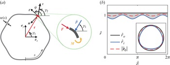
 a
a p¯
p¯ v
v b
b r^=2r/D
 s^
s^ w(s^)
w(s^) n0=3
n0=3
 a
a p^
p^ Δt^=
Δt^= 4×10⁻⁴
 /τ
/τ p^
p^ t^
t^ b
b Γ
Γ t^
t^ p^
p^
 a
a D=80
D=80 p¯max=1800
 α=0.31
 T=111
T=111 b
b n
n Eb
Eb a
a n
n Eb
Eb tN
tN tE
tE c
c tE/tP
tE/tP tN/tP
tN/tP tE/tP=tN/tP
 tN/tP=1
 a
a D=60
D=60 p¯max=1020
 α=0.5
α=0.5 T=87
T=87 t=tN
t=tN t=tE
t=tE b
b n
n c
c Eb
Eb d
d p¯
p¯ a
a p¯und
p¯und
 a
a p^max
p^max t^P
t^P nmax
nmax p^und
p^und b
b nmax
nmax p^max
p^max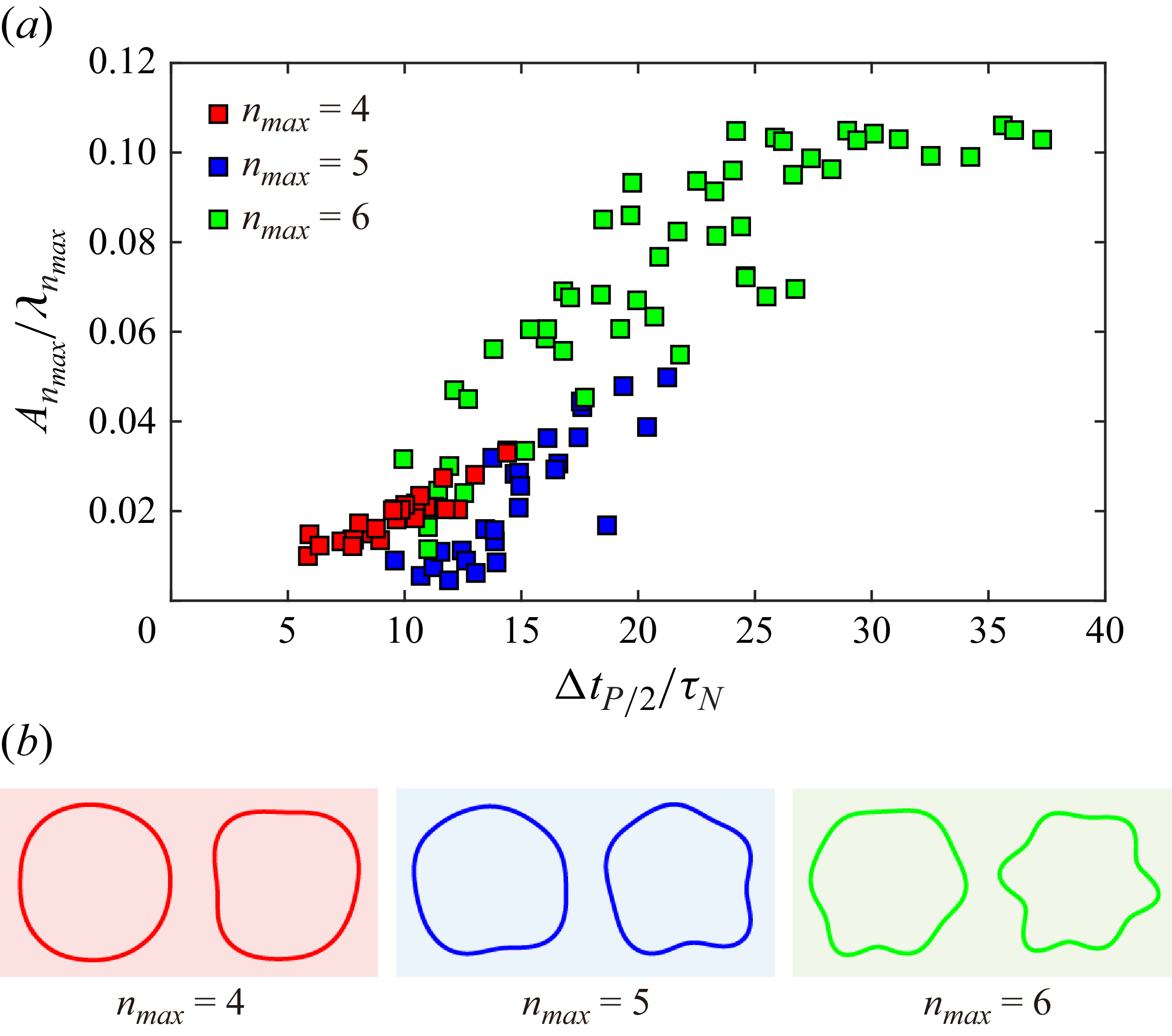
 a
a Anmax/λnmax
 nmax
nmax ΔtP/2/τN
 b
b Anmax/λnmax
 Anmax/λnmax
 nmax
nmax Anmax/λnmax
 0.010
0.010 0.033
0.033 nmax=4
 0.021
0.021 0.050
0.050 nmax=5
 0.047
0.047 0.103
0.103 nmax=6
 a
a w
w n0=3
n0=3 D=50
D=50 wuni=1.3
 Δw^=0.21
 p^max=110
 α=0.2
α=0.2 T=107
T=107 b
b Anmax/λnmax
 Δw^
Δw^ n0=3
n0=3 D=60
D=60 wuni=1.2
 p^max
p^max α
α α=0.5
α=0.5 Δκ^0
Δκ^0 Δw^
Δw^


 Open access

