





1. Introduction
In the case of moderate to severe aortic stenosis, the native aortic valve can be replaced surgically or percutaneously by a prosthesis. Surgical aortic valve prostheses can be categorised into mechanical heart valves (MHVs) and bioprosthetic heart valves (BHVs). While MHVs provide superior durability paired with the significant disadvantage of lifelong anti-coagulation therapy (Yun et al. Reference Yun, Dasi, Aidun and Yoganathan2014; Hedayat, Asgharzadeh & Borazjani Reference Hedayat, Asgharzadeh and Borazjani2017; Klusak & Quinlan Reference Klusak and Quinlan2019), the design of the BHV creates a much more physiological flow field without the need for anti-coagulation medication. However, turbulent flow during peak systole (Becsek, Pietrasanta & Obrist Reference Becsek, Pietrasanta and Obrist2020) is conjectured to contribute to the two failure modes of biological tissue valves made of porcine or bovine pericardium, resulting in a durability of $10$
to
$10$
to $15$
years (Kheradvar et al. Reference Kheradvar2015): (a) leaflet thrombosis (Egbe et al. Reference Egbe, Pislaru, Pellikka, Poterucha, Schaff, Maleszewski and Connolly2015; Holmes & Mack Reference Holmes and Mack2017; Puri, Auffret & Rodés-Cabau Reference Puri, Auffret and Rodés-Cabau2017) and (b) structural valve deterioration (Dvir et al. Reference Dvir2018; Gomel, Lee & Grande-Allen Reference Gomel, Lee and Grande-Allen2019; Li Reference Li2019; Tsolaki et al. Reference Tsolaki2023). Although various experimental studies (Saikrishnan et al. Reference Reul, Vahlbruch, Giersiepen, Schmitz-Rode, Hirtz and Effert2012; Hasler & Obrist Reference Haj-Ali, Marom, Zekry, Rosenfeld and Raanani2018; Jahren et al. Reference Huerre and Monkewitz2018; Oechtering et al. Reference Nordström, Nordin and Henningson2019; Lee et al. Reference Klusak and Quinlan2020; Ferrari & Obrist Reference Egbe, Pislaru, Pellikka, Poterucha, Schaff, Maleszewski and Connolly2024) as well as numerical studies (Borazjani Reference Becsek, Pietrasanta and Obrist2013; Bavo et al. Reference Bagheri, Schlatter, Schmid and Henningson2016; de Tullio & Pascazio Reference Tsolaki2016; Hedayat et al. Reference Hedayat, Asgharzadeh and Borazjani2017; Chen & Luo Reference Bornemann and Obrist2018; Becsek et al. Reference Becsek, Pietrasanta and Obrist2020; Kaiser et al. Reference Johnson, Wu, Xu, Wiese, Rajanna, Herrema, Ganapathysubramanian, Hughes, Sacks and Hsu2021; Gallo et al. Reference Fischer, Lottes and Kerkemeier2022; Johnson et al. Reference Jeong, Hussain, Schoppa and Kim2022; Asadi & Borazjani Reference Åkervik, Brandt, Henningson, Hœpffner, Marxen and Schlatter2023) investigated both fluid and structural motion, the temporal and spatial onset of laminar-transition mechanisms remain poorly understood for the flow around BHVs. One reason is the complex dynamics of the underpinning FSI problem. During valve opening, an aortic jet emerges from the valve orifice, forming a starting vortex. While the aortic jet impinges on the aortic wall downstream of the valve and creates retrograde flow, the valve leaflets either start oscillating periodically, so-called fluttering, or remain stable in an open position. The occurrence and intensity of fluttering is generally suspected to be connected to downstream turbulence, valve design and flow patterns within the sinus portions surrounding the leaflets. In addition, leaflet material, leaflet thickness and valve sizing might play a role in leaflet fluttering (Chen & Luo Reference Chen and Luo2020; Johnson et al. Reference Johnson, Rajanna, Yang and Hsu2020; Lee et al. Reference Lee, Rygg, Kolahdouz, Rossi, Retta, Duraiswamy, Scotten, Craven and Griffith2021).
$15$
years (Kheradvar et al. Reference Kheradvar2015): (a) leaflet thrombosis (Egbe et al. Reference Egbe, Pislaru, Pellikka, Poterucha, Schaff, Maleszewski and Connolly2015; Holmes & Mack Reference Holmes and Mack2017; Puri, Auffret & Rodés-Cabau Reference Puri, Auffret and Rodés-Cabau2017) and (b) structural valve deterioration (Dvir et al. Reference Dvir2018; Gomel, Lee & Grande-Allen Reference Gomel, Lee and Grande-Allen2019; Li Reference Li2019; Tsolaki et al. Reference Tsolaki2023). Although various experimental studies (Saikrishnan et al. Reference Reul, Vahlbruch, Giersiepen, Schmitz-Rode, Hirtz and Effert2012; Hasler & Obrist Reference Haj-Ali, Marom, Zekry, Rosenfeld and Raanani2018; Jahren et al. Reference Huerre and Monkewitz2018; Oechtering et al. Reference Nordström, Nordin and Henningson2019; Lee et al. Reference Klusak and Quinlan2020; Ferrari & Obrist Reference Egbe, Pislaru, Pellikka, Poterucha, Schaff, Maleszewski and Connolly2024) as well as numerical studies (Borazjani Reference Becsek, Pietrasanta and Obrist2013; Bavo et al. Reference Bagheri, Schlatter, Schmid and Henningson2016; de Tullio & Pascazio Reference Tsolaki2016; Hedayat et al. Reference Hedayat, Asgharzadeh and Borazjani2017; Chen & Luo Reference Bornemann and Obrist2018; Becsek et al. Reference Becsek, Pietrasanta and Obrist2020; Kaiser et al. Reference Johnson, Wu, Xu, Wiese, Rajanna, Herrema, Ganapathysubramanian, Hughes, Sacks and Hsu2021; Gallo et al. Reference Fischer, Lottes and Kerkemeier2022; Johnson et al. Reference Jeong, Hussain, Schoppa and Kim2022; Asadi & Borazjani Reference Åkervik, Brandt, Henningson, Hœpffner, Marxen and Schlatter2023) investigated both fluid and structural motion, the temporal and spatial onset of laminar-transition mechanisms remain poorly understood for the flow around BHVs. One reason is the complex dynamics of the underpinning FSI problem. During valve opening, an aortic jet emerges from the valve orifice, forming a starting vortex. While the aortic jet impinges on the aortic wall downstream of the valve and creates retrograde flow, the valve leaflets either start oscillating periodically, so-called fluttering, or remain stable in an open position. The occurrence and intensity of fluttering is generally suspected to be connected to downstream turbulence, valve design and flow patterns within the sinus portions surrounding the leaflets. In addition, leaflet material, leaflet thickness and valve sizing might play a role in leaflet fluttering (Chen & Luo Reference Chen and Luo2020; Johnson et al. Reference Johnson, Rajanna, Yang and Hsu2020; Lee et al. Reference Lee, Rygg, Kolahdouz, Rossi, Retta, Duraiswamy, Scotten, Craven and Griffith2021).
In a previous study of the two-dimensional flow field (Bornemann & Obrist Reference Borazjani2024), the onset of valve fluttering could be related to an absolute shear-layer instability initiated by a secondary vortex emerging from the interaction between a starting vortex and the aortic wall. A fluid-structure interaction instability of the leaflets was triggered by the upstream travelling hydrodynamic instability which occurred without the contribution of FSI. In Bornemann & Obrist (Reference Borazjani2024), leaflet oscillations of increasing amplitude led to vortex shedding and secondary shear-layer instabilities.
In a following study (Bornemann & Obrist Reference Bornemann and Obrist2025), we increased the model complexity by simulating the three-dimensional fluid-structure interaction between the valve, the aortic wall and the blood flow. Here, the absence of leaflet fluttering resulted in lower turbulent kinetic energy (TKE) levels in the immediate vicinity of the valve. In the presence of fluttering, peaks in the TKE occur close to the valve; however, values decrease gradually with streamwise distance while a non-fluttering valve yields the opposite trend. In terms of vortex development and breakdown to turbulence, we observed a three-lobed starting vortex followed by periodically shed secondary vortices due to the oscillating leaflet motion of the fluttering valve. The non-fluttering design created a six-lobed starting vortex which broke down to small-scale structures much faster. This previous study focused on the quantitative description of vortex development and breakdown and the relation of observed phenomena to clinically relevant parameters such as TKE, sinus washout and viscous shear stresses.
The present study aims to investigate this very complex vortex breakdown, and to identify the unstable modes during systolic acceleration in an effort to understand the instabilities responsible for the onset of laminar–turbulent transition.
While global stability analysis is an established tool for the identification of global eigenmodes for canonical, and even complex-geometry, cases, the transient flow past a BHV, which is highly influenced by its interaction with the valve structure, presents a novel and challenging configuration for a carefully tailored, quantitative analysis. Breaking down our problem to a more simplified flow configuration, while neglecting FSI, the flow field in the ascending aorta past the BHV can be characterised as a confined jet in a compliant pipe. In an unconfined jet flow, regions of local absolute instability can initiate global shear instabilities (Huerre & Monkewitz Reference Holzapfel, Gasser and Ogden1990) which are subsequently enhanced by the presence of walls (Poole & Turner Reference Peplinski, Schlatter, Fischer and Henningson2023). The evolution from a convective shear-layer instability to an absolute instability is promoted by the interaction between shear layers (Yu & Monkewitz Reference Vennemann, Rösgen, Heinisch and Obrist1990). In the case of a rigid wall, only a shear-induced mode exists, which is modified and accompanied by a wall-induced mode when introducing compliant walls as given in the cardiovascular system. While in Bornemann & Obrist (Reference Bornemann and Obrist2025) stronger confinement of the aortic jet led to quicker re-laminarisation of the flow past the BHV, Poole & Turner (Reference Peplinski, Schlatter, Fischer and Henningson2023) found both stabilising and destabilising effects of the compliant wall on the flow.
In contrast to the described simplified configurations, laminar–turbulent transition past the BHV occurs during systolic acceleration, i.e. the ejection phase of the heart when the ventricle contracts and the valve opens. During this temporal window, the inflow rate gradually increases. Evaluating a mean flow field or exploiting periodicity (i.e. Floquet theory) in the analysis of base flows is therefore not an option. As a first step in breaking down the complex flow field in the ascending aorta, we apply a moving-average approach in which the flow is temporally averaged over shifting smaller intervals within the time window of interest during systolic acceleration. After creating base flows for each time interval, three-dimensional global eigenmodes are found for both a fluttering and non-fluttering valve designs in three distinct selected time windows. In this way, the present study aims to evaluate the global instabilities present for both the fluttering and non-fluttering cases. Then, the transient growth of global modes is studied using optimal perturbation theory. In this manner, we assess the hypothesis that optimal perturbations of the shear layer for both valves are linked to the onset of transition from laminar to turbulent fluid motion.
2. Numerical fluid-structure interaction simulations
2.1. Governing equations and numerical method
A high-fidelity GPU-accelerated FSI solver developed for biomedical applications is used for simulating the interaction between valve and blood flow on hybrid high-performance computing platforms (Nestola et al. Reference Maday, Patera and Ronquist2019; Zolfaghari & Obrist Reference Yun, Dasi, Aidun and Yoganathan2021). The incompressible Navier–Stokes equations are solved by a direct numerical simulation (DNS) approach (Henniger, Obrist & Kleiser Reference Hedayat, Asgharzadeh and Borazjani2010)
 \begin{align} \rho _{\!f} \frac {\partial \boldsymbol{u}_{\!f}}{\partial t} + \rho _{\!f} \left (\boldsymbol{u}_{\!f}\boldsymbol{\cdot }\boldsymbol{\nabla }\right ) \boldsymbol{u}_{\!f} &= -\boldsymbol{\nabla }\!p_{\!f} + \mu _{\!f} {\nabla} ^2 \boldsymbol{u}_{\!f} + \boldsymbol{f}_{\!\textit{FSI}}, \end{align}
 \begin{align} \boldsymbol{\nabla }\boldsymbol{\cdot }\boldsymbol{u}_{\!f} &= 0, \end{align}
with the three-dimensional velocity field $\boldsymbol{u}_{\!f} = [u_{f,x},u_{f,y},u_{f,z} ]^T$
, pressure
$\boldsymbol{u}_{\!f} = [u_{f,x},u_{f,y},u_{f,z} ]^T$
, pressure $p_{\!f}$
, fluid density
$p_{\!f}$
, fluid density $\rho _{\!f}$
and fluid dynamic viscosity
$\rho _{\!f}$
and fluid dynamic viscosity $\mu _{\!f}$
. This high-order Navier–Stokes solver uses a third-order Runge–Kutta time stepping scheme for temporal discretisation and a sixth-order finite-difference scheme for spatial discretisation.
$\mu _{\!f}$
. This high-order Navier–Stokes solver uses a third-order Runge–Kutta time stepping scheme for temporal discretisation and a sixth-order finite-difference scheme for spatial discretisation.
Structural motions of the valve leaflets, valve stent and aortic wall are modelled using the full elastodynamic equations in their weak form
 \begin{align} \rho _s \frac {\partial \boldsymbol{u}_s}{\partial t} - \boldsymbol{\nabla }\boldsymbol{\cdot }\boldsymbol{P} &= 0, \end{align}
with the displacement field $\boldsymbol{u}_s = [u_{s,x},u_{s,y},u_{s,z} ]^T$
, the structural density
$\boldsymbol{u}_s = [u_{s,x},u_{s,y},u_{s,z} ]^T$
, the structural density $\rho _s$
and the Piola–Kirchhoff tensor
$\rho _s$
and the Piola–Kirchhoff tensor $\boldsymbol{P}$
.
$\boldsymbol{P}$
.
Fluid and structural motion are coupled by a modified immersed boundary method based on variational transfer (Nestola et al. Reference Maday, Patera and Ronquist2019). The interface conditions are described as
 \begin{align} \boldsymbol{u}_{\!f} &= \frac {\partial \boldsymbol{u}_s}{\partial t}, \end{align}
 \begin{align} J^{-1} \boldsymbol{P}\!\boldsymbol{F}^T \boldsymbol{n} &= \boldsymbol{\sigma _{\!f}} \boldsymbol{n}, \end{align}
with the deformation gradient $\boldsymbol{F} = \boldsymbol{\nabla }\boldsymbol{u}_s + \boldsymbol{I}$
, its identity matrix
$\boldsymbol{F} = \boldsymbol{\nabla }\boldsymbol{u}_s + \boldsymbol{I}$
, its identity matrix $\boldsymbol{I}$
and its respective determinant
$\boldsymbol{I}$
and its respective determinant $J = \text{det} \boldsymbol{F}$
. The Cauchy stress of the fluid is defined by
$J = \text{det} \boldsymbol{F}$
. The Cauchy stress of the fluid is defined by $\boldsymbol{\sigma _{\!f}},$ $\boldsymbol{n}$
denotes the unit normal vector to the structural surface. Further details about numerical schemes and the FSI approach can be found in Nestola et al. (Reference Maday, Patera and Ronquist2019) and Becsek et al. (Reference Becsek, Pietrasanta and Obrist2020).
$\boldsymbol{n}$
denotes the unit normal vector to the structural surface. Further details about numerical schemes and the FSI approach can be found in Nestola et al. (Reference Maday, Patera and Ronquist2019) and Becsek et al. (Reference Becsek, Pietrasanta and Obrist2020).
The rectangular fluid domain is sized at $0.045\,\textrm{m}\, \times \, 0.045\,\textrm{m}\, \times \, 0.103\,\textrm{m}$
and discretised by a rectilinear structured grid of
$0.045\,\textrm{m}\, \times \, 0.045\,\textrm{m}\, \times \, 0.103\,\textrm{m}$
and discretised by a rectilinear structured grid of $193 \times 193 \times 513$
elements. The minimum element length is reduced to approximately
$193 \times 193 \times 513$
elements. The minimum element length is reduced to approximately $125\,{\unicode{x03BC}} \textrm{m},$
by a grid stretching approach. The finest resolution is located in the region close to the valve, ensuring sufficient resolution for capturing the onset of instabilities. The structural domain (aortic wall, valve stent, valve leaflets) is resolved by approximately
$125\,{\unicode{x03BC}} \textrm{m},$
by a grid stretching approach. The finest resolution is located in the region close to the valve, ensuring sufficient resolution for capturing the onset of instabilities. The structural domain (aortic wall, valve stent, valve leaflets) is resolved by approximately $450\,000$
tetrahedral elements.
$450\,000$
tetrahedral elements.
Numerical simulations are performed on a Cray XC40/XC50 high-performance cluster with a time step size of $2.5\boldsymbol{\times }10^{-6}\, \textrm{s}$
resulting in around
$2.5\boldsymbol{\times }10^{-6}\, \textrm{s}$
resulting in around $21\,500$
node hours on
$21\,500$
node hours on $32$
nodes for the systolic acceleration phase with a physical duration of
$32$
nodes for the systolic acceleration phase with a physical duration of $0.2\,\textrm{s}$
.
$0.2\,\textrm{s}$
.
2.2. Problem set-up
The fluid is modelled as incompressible and Newtonian with material properties comparable to blood (density $\rho _{\!f} = 1050\,\textrm{kg} \, \textrm{m}^{-3}$
, dynamic viscosity
$\rho _{\!f} = 1050\,\textrm{kg} \, \textrm{m}^{-3}$
, dynamic viscosity $\mu _{\!f} = 0.004\, \textrm{Pa s}$
). The structural domain is generally divided into aortic wall, valve stent and three valve leaflets. Two valves with distinct stent and leaflet geometries, leading to fluttering and non-fluttering leaflet kinematics, are shown in figure 1. The aortic wall and valve stent are modelled as linearly elastic, exhibiting a nearly rigid behaviour with negligible wall displacement. The constitutive behaviour of the biological, flexible leaflets is modelled by a fibre-reinforced hyper-elastic Holzapfel–Gasser–Ogden model (Holzapfel, Gasser & Ogden Reference Holmes and Mack2000). An angle of
$\mu _{\!f} = 0.004\, \textrm{Pa s}$
). The structural domain is generally divided into aortic wall, valve stent and three valve leaflets. Two valves with distinct stent and leaflet geometries, leading to fluttering and non-fluttering leaflet kinematics, are shown in figure 1. The aortic wall and valve stent are modelled as linearly elastic, exhibiting a nearly rigid behaviour with negligible wall displacement. The constitutive behaviour of the biological, flexible leaflets is modelled by a fibre-reinforced hyper-elastic Holzapfel–Gasser–Ogden model (Holzapfel, Gasser & Ogden Reference Holmes and Mack2000). An angle of $60^\circ$
is set between two fibre sets in each leaflet, and material parameters are chosen according to the study of Auricchio et al. (Reference Asadi and Borazjani2014). Two valve geometries are inserted into the generic aortic root defined according to the studies of Reul et al. (Reference Puri, Auffret and Rodés-Cabau1990) and Haj-Ali et al. (Reference Gomel, Lee and Grande-Allen2012). The fluttering valve (figure 1
a, left) resembles the Intuity Elite (Edwards Lifesciences) of size
$60^\circ$
is set between two fibre sets in each leaflet, and material parameters are chosen according to the study of Auricchio et al. (Reference Asadi and Borazjani2014). Two valve geometries are inserted into the generic aortic root defined according to the studies of Reul et al. (Reference Puri, Auffret and Rodés-Cabau1990) and Haj-Ali et al. (Reference Gomel, Lee and Grande-Allen2012). The fluttering valve (figure 1
a, left) resembles the Intuity Elite (Edwards Lifesciences) of size $21\, \textrm{mm}$
and exhibits a periodic oscillatory motion of the leaflets during systole, as shown in previous studies (Becsek et al. Reference Becsek, Pietrasanta and Obrist2020; Bornemann & Obrist Reference Bornemann and Obrist2025). The fluttering frequency of this valve design was also confirmed in experimental studies of Jahren et al. (Reference Jahren, Heinisch, Hasler, Winkler, Stortecky, Pilgrim, Londono, Carrel, Tengg-Kobligk and Obrist2026). The non-fluttering valve model (figure 1
a, right) is re-constructed according to a computed tomography (CT) scan of the Carpentier–Edwards PERIMOUNT Magna Ease (Edwards Lifesciences) of size
$21\, \textrm{mm}$
and exhibits a periodic oscillatory motion of the leaflets during systole, as shown in previous studies (Becsek et al. Reference Becsek, Pietrasanta and Obrist2020; Bornemann & Obrist Reference Bornemann and Obrist2025). The fluttering frequency of this valve design was also confirmed in experimental studies of Jahren et al. (Reference Jahren, Heinisch, Hasler, Winkler, Stortecky, Pilgrim, Londono, Carrel, Tengg-Kobligk and Obrist2026). The non-fluttering valve model (figure 1
a, right) is re-constructed according to a computed tomography (CT) scan of the Carpentier–Edwards PERIMOUNT Magna Ease (Edwards Lifesciences) of size $21\, \textrm{mm}$
. Flow fields and leaflet kinematics were validated experimentally in a study of Ferrari & Obrist (Reference Egbe, Pislaru, Pellikka, Poterucha, Schaff, Maleszewski and Connolly2024). A total of
$21\, \textrm{mm}$
. Flow fields and leaflet kinematics were validated experimentally in a study of Ferrari & Obrist (Reference Egbe, Pislaru, Pellikka, Poterucha, Schaff, Maleszewski and Connolly2024). A total of $409$
DICOM images with a spacing of
$409$
DICOM images with a spacing of $34.4\,{\unicode{x03BC}} \textrm{m}$
between slices is extracted by a microCT 100 scanner (Scanco Medical AG, Switzerland). Geometrical variations between the individual leaflets are adjusted to ensure symmetry of the three leaflets. The leaflets of both valve designs have a thickness of
$34.4\,{\unicode{x03BC}} \textrm{m}$
between slices is extracted by a microCT 100 scanner (Scanco Medical AG, Switzerland). Geometrical variations between the individual leaflets are adjusted to ensure symmetry of the three leaflets. The leaflets of both valve designs have a thickness of $500\,{\unicode{x03BC}} \textrm{m}.$
(a) Fluttering (F, left of a) and non-fluttering (NF, right of a) valve geometry inserted in a generic aortic root. (b) Flow rate over time within time period of interest $t = [0.04;0.08]$
s. (c) Region of interest in cylindrical aortic domain above the sinotubular junction (STJ).
$t = [0.04;0.08]$
s. (c) Region of interest in cylindrical aortic domain above the sinotubular junction (STJ).

Applying a fringe region technique as described in Nordström et al. (Reference Nestola, Becsek, Zolfaghari, Zulian, De Marinis, Krause and Obrist1999), a penalisation term $\boldsymbol{f}_{\textit{fringe}} (\boldsymbol{x} )$
is added to the right-hand side of the Navier–Stokes equations within a specified inflow and outflow region. This way, an average systolic transvalvular pressure gradient is prescribed while simultaneously suppressing lateral velocity components, dampening incoming perturbations due to the periodic fluid domain. This approach creates a physiological inflow that mimics the systolic acceleration phase while pressurising the aortic root, in close accordance with physiological conditions.
$\boldsymbol{f}_{\textit{fringe}} (\boldsymbol{x} )$
is added to the right-hand side of the Navier–Stokes equations within a specified inflow and outflow region. This way, an average systolic transvalvular pressure gradient is prescribed while simultaneously suppressing lateral velocity components, dampening incoming perturbations due to the periodic fluid domain. This approach creates a physiological inflow that mimics the systolic acceleration phase while pressurising the aortic root, in close accordance with physiological conditions.
After the initial opening phase of the valve, lasting approximately $20\, \textrm{ms},$
the valve remains in an open position (while potentially exhibiting oscillations), until it closes asynchronously at a third of one cardiac cycle corresponding to approximately
$20\, \textrm{ms},$
the valve remains in an open position (while potentially exhibiting oscillations), until it closes asynchronously at a third of one cardiac cycle corresponding to approximately $0.3\, \textrm{s}$
(Vennemann et al. Reference de Tullio and Pascazio2018). The physical time of the presented numerical simulations is set to
$0.3\, \textrm{s}$
(Vennemann et al. Reference de Tullio and Pascazio2018). The physical time of the presented numerical simulations is set to $0.2\, \textrm{s},$
as laminar–turbulent transition is expected during the early systole (Becsek et al. Reference Becsek, Pietrasanta and Obrist2020). At this point, a flow rate of
$0.2\, \textrm{s},$
as laminar–turbulent transition is expected during the early systole (Becsek et al. Reference Becsek, Pietrasanta and Obrist2020). At this point, a flow rate of $14\, \textrm{min}^{-1}$
is reached.
$14\, \textrm{min}^{-1}$
is reached.
3. Volume-filtered transient vortical structures
Initial analysis of predominant vortical structures and vortex breakdown reveals the time period of $ [0.04,0.08 ]\, \textrm{s}$
(see figure 1
b) as the most relevant for further investigations. To this end, the flow field is first smoothed by calculating a moving average
$ [0.04,0.08 ]\, \textrm{s}$
(see figure 1
b) as the most relevant for further investigations. To this end, the flow field is first smoothed by calculating a moving average
 \begin{equation} \overline {\boldsymbol{u}}_{f,i} = \frac {1}{n} \sum _{k=i-n+1}^{i} \boldsymbol{u}_{f,k}, \end{equation}
with $n = 200$
instantaneous snapshots per interval, and a total of
$n = 200$
instantaneous snapshots per interval, and a total of $1600$
snapshots covering the full time interval
$1600$
snapshots covering the full time interval $[0.04, 0.08]\,\textrm{s}$
. The index
$[0.04, 0.08]\,\textrm{s}$
. The index $i$
advances in increments of
$i$
advances in increments of $40$
snapshots for each averaged field, resulting in
$40$
snapshots for each averaged field, resulting in $i \in \{200, 240, 280, \ldots , 1600\}$
.
$i \in \{200, 240, 280, \ldots , 1600\}$
.
For each moving-averaged flow field, the $\lambda _2$
-criterion (Jeong et al. Reference Jahren, Vennemann, Bornemann, Rösgen and Obrist1997) is computed. Iso-surfaces of the
$\lambda _2$
-criterion (Jeong et al. Reference Jahren, Vennemann, Bornemann, Rösgen and Obrist1997) is computed. Iso-surfaces of the $\lambda _2$
-criterion are extracted and the enclosed volumes are calculated. Subsequently, the individual volumes are ranked by volume size, and volumes below a certain threshold are discarded. Hereby, spurious vortical structures originating from numerical artefacts at the immersed boundary, but also smaller vortices irrelevant for the dominant mechanisms of vortex breakdown, can be excluded from further analysis. This approach enables a clearer focus on the fundamental mechanisms of vortex development.
$\lambda _2$
-criterion are extracted and the enclosed volumes are calculated. Subsequently, the individual volumes are ranked by volume size, and volumes below a certain threshold are discarded. Hereby, spurious vortical structures originating from numerical artefacts at the immersed boundary, but also smaller vortices irrelevant for the dominant mechanisms of vortex breakdown, can be excluded from further analysis. This approach enables a clearer focus on the fundamental mechanisms of vortex development.
The resulting vortical structures are displayed for the fluttering valve in figure 2 and for the non-fluttering valve in figure 3 for consecutive moving-average time periods of $\Delta t = 0.005\,\textrm{s}$
in the intervals
$\Delta t = 0.005\,\textrm{s}$
in the intervals $t \in [0.040, 0.045]\,\textrm{s}, t \in [0.050, 0.055]\,\textrm{s}, t \in [0.055, 0.060]\,\textrm{s}, t \in [0.060, 0.065]\,\textrm{s}$
and
$t \in [0.040, 0.045]\,\textrm{s}, t \in [0.050, 0.055]\,\textrm{s}, t \in [0.055, 0.060]\,\textrm{s}, t \in [0.060, 0.065]\,\textrm{s}$
and $t \in [0.065, 0.070]\,\textrm{s}$
.
$t \in [0.065, 0.070]\,\textrm{s}$
.
Volume-filtered moving-averaged $\lambda _2$
-criterion iso-surfaces for the fluttering valve, coloured by the streamwise velocity component, for the following time periods (from left to right):
$\lambda _2$
-criterion iso-surfaces for the fluttering valve, coloured by the streamwise velocity component, for the following time periods (from left to right): $t \in [0.040, 0.045]\,\textrm{s},$ $t \in [0.050, 0.055]\,\textrm{s},$ $t \in [0.055, 0.060]\,\textrm{s},$ $t \in [0.060, 0.065]\,\textrm{s}$
and
$t \in [0.060, 0.065]\,\textrm{s}$
and $t \in [0.065, 0.070]\,\textrm{s}$
.
$t \in [0.065, 0.070]\,\textrm{s}$
.

Volume-filtered moving-averaged $\lambda _2$
-criterion iso-surfaces for the non-fluttering valve, coloured by the streamwise velocity component, for the following time periods:
$\lambda _2$
-criterion iso-surfaces for the non-fluttering valve, coloured by the streamwise velocity component, for the following time periods: $t \in [0.040, 0.045]\,\textrm{s},$ $t \in [0.050, 0.055]\,\textrm{s},$ $t \in [0.055, 0.060]\,\textrm{s},$ $t \in [0.060, 0.065]\,\textrm{s}$
and
$t \in [0.060, 0.065]\,\textrm{s}$
and $t \in [0.065, 0.070]\,\textrm{s}$
.
$t \in [0.065, 0.070]\,\textrm{s}$
.

For both valves, a starting vortex is formed immediately downstream of the valve. Depending on the shape of the valve orifice, this vortex appears in a triangular or hexagonal shape for the fluttering or non-fluttering valve, respectively. We already notice the rise of three-dimensionality in the vortex, as the iso-surfaces above the valve post appear distorted in the streamwise direction. Only for the fluttering valve do we additionally observe a complex secondary vortical structure above the valve post with two vortex lines wrapping around the corners of the primary triangular starting vortex. During systolic acceleration, the starting vortex is advected downstream, passing the STJ into the ascending aorta. Because of the radial confinement of the flow field by the aortic wall and its no-slip condition, each lobe of the starting vortex bends downwards. The fluttering valve also exhibits pronounced streamwise vortices of opposite rotation, originating from the leaflet gap at the valve post and connected to the secondary structures wrapped around the corners of the starting vortex. These hyperbolic vortices remain connected to the starting vortex during its downstream advection and elongate during this process. For the non-fluttering valve this flow feature is only marginally visible. A second vortex is shed from the valve orifice of both valves – caused by two different mechanisms for fluttering and non-fluttering valves. For the fluttering valve, the leaflets undergo a periodic whiplash motion at a distinct frequency of $40\,\textrm{Hz}$
which results in periodic vortex shedding at the same frequency. In case of the non-fluttering valve, only one vortex is shed due to flow separation at the curved leaflet shape. Both kinds of secondary vortices exhibit a faster advection speed and eventually pass through the starting vortex. In general, the triangular starting vortex, the periodic vortex shedding and the existence of counter-rotating hyperbolic vortices above the valve posts yield far richer flow structures in the ascending aorta past the fluttering valve. The flow field past a non-fluttering valve is limited to one distinct starting vortex, a second smaller, but faster, vortex and small-scale vortical structures caused by flow separation at the leaflet.
$40\,\textrm{Hz}$
which results in periodic vortex shedding at the same frequency. In case of the non-fluttering valve, only one vortex is shed due to flow separation at the curved leaflet shape. Both kinds of secondary vortices exhibit a faster advection speed and eventually pass through the starting vortex. In general, the triangular starting vortex, the periodic vortex shedding and the existence of counter-rotating hyperbolic vortices above the valve posts yield far richer flow structures in the ascending aorta past the fluttering valve. The flow field past a non-fluttering valve is limited to one distinct starting vortex, a second smaller, but faster, vortex and small-scale vortical structures caused by flow separation at the leaflet.
4. Base flows across transient systolic acceleration
4.1. Definition of inlet conditions and numerical set-up
As the flow downstream of a BHV is not only highly influenced by the interaction with the flexible valve tissue but also undergoes acceleration during the systolic ejection phase, the extraction of base flows is rather complex. To enable the global stability analysis of base flows at different phases during systolic acceleration, we simplify the problem by only considering the cylindrical aortic domain downstream of the valve (diameter $d=0.01375\,\textrm{m}$
and streamwise length
$d=0.01375\,\textrm{m}$
and streamwise length $h=0.05\,\textrm{m}$
) for further analysis (figure 1
c).
$h=0.05\,\textrm{m}$
) for further analysis (figure 1
c).
Nonlinear DNSs are set up within the open-source spectral-element code Nek5000 (Fischer et al. Reference Ferrari and Obrist2008) which solves the incompressible Navier–Stokes equations by a Galerkin projection scheme for each spectral element. A $\mathbb{P}_N$
-
$\mathbb{P}_N$
- $\mathbb{P}_{N-2}$
-formalism (Maday & Patera Reference Li1989) is used, expressing velocity as a linear combination of
$\mathbb{P}_{N-2}$
-formalism (Maday & Patera Reference Li1989) is used, expressing velocity as a linear combination of $N$
th-order Lagrangian basis functions based on Gauss–Lobatto–Legendre points and pressure by Lagrangian interpolants of order
$N$
th-order Lagrangian basis functions based on Gauss–Lobatto–Legendre points and pressure by Lagrangian interpolants of order $N-2$
based on Gauss–Legendre nodes (Maday, Patera & Ronquist Reference Maday and Patera1987; Maday & Patera Reference Li1989). A third-order backward differentiation scheme, treating the viscous terms implicitly, is used for temporal integration. Aliasing errors are avoided by using over-integration for the nonlinear advection terms.
$N-2$
based on Gauss–Legendre nodes (Maday, Patera & Ronquist Reference Maday and Patera1987; Maday & Patera Reference Li1989). A third-order backward differentiation scheme, treating the viscous terms implicitly, is used for temporal integration. Aliasing errors are avoided by using over-integration for the nonlinear advection terms.
Multiple moving-average flow fields at the cross-section at the STJ are used as an inlet boundary condition for each simulation to obtain base flows corresponding to different time windows (figure 4). We consider moving-average flow fields over the temporal intervals $t \in [0.055, 0.060 ]\,\textrm{s},$ $t \in [0.060, 0.065 ]\,\textrm{s}$
and
$t \in [0.060, 0.065 ]\,\textrm{s}$
and $t \in [0.065, 0.070 ]\,\textrm{s}$
to obtain base flows for three successive time windows. These time windows correspond to the first intervals in which vortical structures shed from the valve (following the initial ring vortex) are observed in DNS in both cases (see figures 2 and 3).
$t \in [0.065, 0.070 ]\,\textrm{s}$
to obtain base flows for three successive time windows. These time windows correspond to the first intervals in which vortical structures shed from the valve (following the initial ring vortex) are observed in DNS in both cases (see figures 2 and 3).
Moving-averaged streamwise velocity profiles (coloured in velocity component $u_{f,z}$
) at inlet ( = STJ) and moving-average valve leaflet shapes (coloured in displacement magnitude
$u_{f,z}$
) at inlet ( = STJ) and moving-average valve leaflet shapes (coloured in displacement magnitude $|\boldsymbol{u}_s|$
) for (a) fluttering and (b) non-fluttering valve. Each velocity profile and leaflet displacement corresponds to the moving-average over the time interval displayed in the bottom row.
$|\boldsymbol{u}_s|$
) for (a) fluttering and (b) non-fluttering valve. Each velocity profile and leaflet displacement corresponds to the moving-average over the time interval displayed in the bottom row.

The temporal time scale of the base flow is defined as $\tau _{\textit{base}} = {Q}/\dot {Q}$
, where
$\tau _{\textit{base}} = {Q}/\dot {Q}$
, where $Q$
is the instantaneous flow rate (see figure 1
b) and
$Q$
is the instantaneous flow rate (see figure 1
b) and $\dot {Q}={\textrm d}Q/{\textrm d}t$
. This time scale represents the characteristic time over which the bulk flow rate changes appreciably relative to its instantaneous magnitude. For the time windows considered here,
$\dot {Q}={\textrm d}Q/{\textrm d}t$
. This time scale represents the characteristic time over which the bulk flow rate changes appreciably relative to its instantaneous magnitude. For the time windows considered here, $\tau _{\textit{base}}$
is of order
$\tau _{\textit{base}}$
is of order $\mathcal{O}(10^{-1})$
s. As will be shown in § 5.3, the characteristic time scales of the unstable perturbations obtained from the stability analysis are much shorter, of order
$\mathcal{O}(10^{-1})$
s. As will be shown in § 5.3, the characteristic time scales of the unstable perturbations obtained from the stability analysis are much shorter, of order $\mathcal{O}(10^{-2})$
s. This separation of time scales indicates that, at each time window, the base flow evolves slowly compared with the instability dynamics, thereby supporting the use of frozen base flows in the subsequent stability analysis. To ensure numerical stability, we eliminate the backflow at the STJ and only consider positive velocity components for the streamwise direction. It should be noted that no significant flow feature was observed in DNS that could be linked to the presence of the backflow region; thus, eliminating the backflow region is not expected to have a significant effect on the results of the stability analysis in the present study. No-slip conditions are imposed at the rigid wall, and a fringe layer is placed at the outlet. Again, the fluid is assumed to be Newtonian with material properties similar to blood (
$\mathcal{O}(10^{-2})$
s. This separation of time scales indicates that, at each time window, the base flow evolves slowly compared with the instability dynamics, thereby supporting the use of frozen base flows in the subsequent stability analysis. To ensure numerical stability, we eliminate the backflow at the STJ and only consider positive velocity components for the streamwise direction. It should be noted that no significant flow feature was observed in DNS that could be linked to the presence of the backflow region; thus, eliminating the backflow region is not expected to have a significant effect on the results of the stability analysis in the present study. No-slip conditions are imposed at the rigid wall, and a fringe layer is placed at the outlet. Again, the fluid is assumed to be Newtonian with material properties similar to blood ( $\rho _{\!f}=1050\,\textrm{kg m}^{-3}$
and
$\rho _{\!f}=1050\,\textrm{kg m}^{-3}$
and $\mu _{\!f}=0.004\,\textrm{Pa s}$
). The computational fluid domain is discretised using
$\mu _{\!f}=0.004\,\textrm{Pa s}$
). The computational fluid domain is discretised using $1\,28\,128$
spectral elements of polynomial order seven (
$1\,28\,128$
spectral elements of polynomial order seven ( $N=7$
), resulting in approximately
$N=7$
), resulting in approximately $66$
million grid points.
$66$
million grid points.
4.2. Stabilising the flow field to obtain base flows
Initially, steady simulations are run with the laminar solver implemented in ANSYS Fluent. The obtained solution $\boldsymbol{U}_{\textit{st}}$
is used as an initial condition and to define the forcing
$\boldsymbol{U}_{\textit{st}}$
is used as an initial condition and to define the forcing $\boldsymbol{f}_{\textit{fringe}}$
within the fringe layer at the outflow of the form
$\boldsymbol{f}_{\textit{fringe}}$
within the fringe layer at the outflow of the form
 \begin{equation} \boldsymbol{f}_{\textit{fringe}} = \varLambda \left (z\right )\left (\boldsymbol{U}_{\textit{st}} - \boldsymbol{u}\right ), \end{equation}
with $\varLambda (z)$
as the fringe coefficient,
$\varLambda (z)$
as the fringe coefficient, $\boldsymbol{U}_{\textit{st}}$
as the computed steady solution and
$\boldsymbol{U}_{\textit{st}}$
as the computed steady solution and $\boldsymbol{u}$
as the current velocity field. As the flow field is highly unstable, we apply selective frequency damping (SFD) to the nonlinear Navier–Stokes equations
$\boldsymbol{u}$
as the current velocity field. As the flow field is highly unstable, we apply selective frequency damping (SFD) to the nonlinear Navier–Stokes equations
 \begin{align} \rho _{\!f} \frac {\partial \boldsymbol{u}}{\partial t} + \rho _{\!f} \left (\boldsymbol{u} \boldsymbol{\cdot }\boldsymbol{\nabla }\right ) \boldsymbol{u} &= - \boldsymbol{\nabla }\!p +\mu _{\!f} {\nabla} ^2 \boldsymbol{u} + \boldsymbol{f}, \end{align}
 \begin{align} \boldsymbol{\nabla }\boldsymbol{\cdot }\boldsymbol{u} &= 0, \end{align}
to calculate the steady base flow $\boldsymbol{U}=[U_x,U_y,U_z]^T$
about which we linearise the Navier–Stokes equations. The SFD was proposed by Åkervik et al. (Reference Åkervik, Brandt, Henningson, Hœpffner, Marxen and Schlatter2006) to obtain steady states of the Navier–Stokes equations by damping unsteady oscillations with a temporal low-pass filter.
$\boldsymbol{U}=[U_x,U_y,U_z]^T$
about which we linearise the Navier–Stokes equations. The SFD was proposed by Åkervik et al. (Reference Åkervik, Brandt, Henningson, Hœpffner, Marxen and Schlatter2006) to obtain steady states of the Navier–Stokes equations by damping unsteady oscillations with a temporal low-pass filter.
An estimate of the global mode frequency, required as an input to the SFD algorithm, has been obtained by performing preliminary nonlinear DNSs; it suggests a dominant oscillation period of $T \approx 0.02\,\textrm{s}$
resulting in a filter width of
$T \approx 0.02\,\textrm{s}$
resulting in a filter width of $\Delta = 2T = 0.04\,\textrm{s}$
and a control cutoff of
$\Delta = 2T = 0.04\,\textrm{s}$
and a control cutoff of $\varTheta =1/ \Delta =25\,\textrm{s}^{-1}.$
Selective frequency damping was capable of stabilising the flow in four out of six flow cases. For the remaining two cases, we applied the BoostConv algorithm proposed by Citro et al. (Reference Citro, Luchini, Giannetti and Auteri2017). The computational cost of the nonlinear simulations is only marginally increased as the algorithm only affects the unstable modes.
4.3. Base flows
Figure 5 shows the streamwise velocity component ( $U_z$
) of the obtained base flows for the moving-window-averaged inlet conditions of
$U_z$
) of the obtained base flows for the moving-window-averaged inlet conditions of $t \in [0.055, 0.060]\,\textrm{s},$ $t \in [0.060, 0.065]\,\textrm{s}$
and
$t \in [0.060, 0.065]\,\textrm{s}$
and $t \in [0.065, 0.070]\,\textrm{s}.$
As the valve orifice area changes periodically for the fluttering valve, an aortic jet of fundamentally different shape is created over time. While the first time window (
$t \in [0.065, 0.070]\,\textrm{s}.$
As the valve orifice area changes periodically for the fluttering valve, an aortic jet of fundamentally different shape is created over time. While the first time window ( $t \in [0.055, 0.060]\,\textrm{s}$
) shows a comparably fast, triangular aortic jet with narrow extensions above the valve posts reaching towards the aortic wall, the second inlet condition (
$t \in [0.055, 0.060]\,\textrm{s}$
) shows a comparably fast, triangular aortic jet with narrow extensions above the valve posts reaching towards the aortic wall, the second inlet condition ( $t \in [0.060, 0.065]\,\textrm{s}$
) leads to an aortic jet with three major arms above the posts and three minor arms above each leaflet. The third inlet profile (
$t \in [0.060, 0.065]\,\textrm{s}$
) leads to an aortic jet with three major arms above the posts and three minor arms above each leaflet. The third inlet profile ( $t \in [0.065, 0.070]\,\textrm{s}$
) creates a complex aortic jet occupying most of the pipe’s cross-section and resulting in less backflow. The first two time windows
$t \in [0.065, 0.070]\,\textrm{s}$
) creates a complex aortic jet occupying most of the pipe’s cross-section and resulting in less backflow. The first two time windows $(t \in [0.055, 0.060]\,\textrm{s}$
and
$(t \in [0.055, 0.060]\,\textrm{s}$
and $t \in [0.060, 0.065]\,\textrm{s}$
) of the non-fluttering valve show a triangular aortic jet extending to the aortic wall with rather high velocity ranges. The third inlet condition (
$t \in [0.060, 0.065]\,\textrm{s}$
) of the non-fluttering valve show a triangular aortic jet extending to the aortic wall with rather high velocity ranges. The third inlet condition ( $t \in [0.065, 0.070]\,\textrm{s}$
), however, produces a more central aortic jet of hexagonal shape.
$t \in [0.065, 0.070]\,\textrm{s}$
), however, produces a more central aortic jet of hexagonal shape.
Base flows for fluttering valve (a) and non-fluttering valve (b) for moving-window-averaged inlet conditions for $t \in [0.055,0.060]\,\textrm{s},$ $t \in [0.060, 0.065]\,\textrm{s}$
and
$t \in [0.060, 0.065]\,\textrm{s}$
and $t \in [0.065, 0.070]\,\textrm{s}$
(from left to right).
$t \in [0.065, 0.070]\,\textrm{s}$
(from left to right).

5. Global stability analysis
5.1. Modal analysis using the Arnoldi algorithm
The governing equations for the perturbations, i.e. $\boldsymbol{u}^{\prime}=[u^{\prime}_x, u^{\prime}_y,u^{\prime}_z]^T$
and
$\boldsymbol{u}^{\prime}=[u^{\prime}_x, u^{\prime}_y,u^{\prime}_z]^T$
and $p^{\prime}$
, are derived by linearising the incompressible Navier–Stokes equations about the obtained base flows
$p^{\prime}$
, are derived by linearising the incompressible Navier–Stokes equations about the obtained base flows $\boldsymbol{U}$
. The linearised Navier–Stokes and continuity equations can be written as
$\boldsymbol{U}$
. The linearised Navier–Stokes and continuity equations can be written as
 \begin{equation} \begin{aligned} \rho _{\!f} \frac {\partial \boldsymbol{u}^{\prime}}{\partial t} + \rho _{\!f} \left (\boldsymbol{u}^{\prime} \boldsymbol{\cdot }\boldsymbol{\nabla }\boldsymbol{U} + \boldsymbol{U} \boldsymbol{\cdot }\boldsymbol{\nabla }\boldsymbol{u}^{\prime}\right ) - \mu _{\!f} {\nabla} ^2 \boldsymbol{u}^{\prime} + \boldsymbol{\nabla }\!p^{\prime} &= \boldsymbol{f}_{\textit{fringe}}, \\ \boldsymbol{\nabla }\boldsymbol{\cdot }\boldsymbol{u}^{\prime} &= 0. \end{aligned} \end{equation}
The right-hand side term $\boldsymbol{f}_{\textit{fringe}}$
forces the perturbations to zero within the last
$\boldsymbol{f}_{\textit{fringe}}$
forces the perturbations to zero within the last $8 \,\%$
of the streamwise (
$8 \,\%$
of the streamwise ( $z$
-direction) extent of the domain, to avoid reflections from the outlet boundary condition. Furthermore, homogeneous Dirichlet boundary conditions are imposed for the velocity perturbations (
$z$
-direction) extent of the domain, to avoid reflections from the outlet boundary condition. Furthermore, homogeneous Dirichlet boundary conditions are imposed for the velocity perturbations ( $\boldsymbol{u}^{\prime}$
) at the inlet of the domain. At the outlet of the domain, the boundary conditions are taken as
$\boldsymbol{u}^{\prime}$
) at the inlet of the domain. At the outlet of the domain, the boundary conditions are taken as
 \begin{equation} \mu _{\!f}\frac {\partial u_z^{\prime}}{\partial z} - p^{\prime} = 0, \qquad \qquad \frac {\partial u_x^{\prime}}{\partial z} = \frac {\partial u_y^{\prime}}{\partial z} = 0. \end{equation}
The perturbation fields $\boldsymbol{u}^{\prime}$
and
$\boldsymbol{u}^{\prime}$
and $p^{\prime}$
follow the ansatz
$p^{\prime}$
follow the ansatz
 \begin{equation} \begin{aligned} \boldsymbol{u}^{\prime}\left (\boldsymbol{x},t\right ) &= \hat {\boldsymbol{u}} \left (\boldsymbol{x}\right ) {\textrm{exp}}\left (-\textrm{i}\lambda t\right ), \\ p^{\prime}\left (\boldsymbol{x},t\right ) &= \hat {p} \left (\boldsymbol{x}\right ) {\textrm{exp}}\left (-\textrm{i} \lambda t\right ), \end{aligned} \end{equation}
where $\boldsymbol{x}=[x,y,z]^T$
, and the growth rate
$\boldsymbol{x}=[x,y,z]^T$
, and the growth rate $\sigma$
and angular frequency
$\sigma$
and angular frequency $\omega$
are deduced from
$\omega$
are deduced from $\lambda = \omega + \textrm{i} \sigma$
.
$\lambda = \omega + \textrm{i} \sigma$
.
Applying the above ansatz to (5.1), we obtain a generalised eigenvalue problem of the form
 \begin{equation} \mathcal{L} \hat {\boldsymbol{q}} = \lambda \mathcal{R}\hat {\boldsymbol{q}}, \end{equation}
with
 \begin{equation} \hat {\boldsymbol{q}}=\begin{pmatrix} \hat {\boldsymbol{u}}\\ \hat {p} \end{pmatrix}\!, \quad \mathcal{R} = \begin{bmatrix} I & 0\\ 0 & 0 \end{bmatrix}, \quad \mathcal{L} = \begin{bmatrix} \rho _{\!f} \left (-\boldsymbol{\nabla }\boldsymbol{U}-\boldsymbol{U} \boldsymbol{\cdot }\boldsymbol{\nabla }\right ) + \mu _{\!f} {\nabla} ^2 & -\boldsymbol{\nabla }\\ \boldsymbol{\nabla }\boldsymbol{\cdot }& 0 \quad \end{bmatrix}\! . \end{equation}
By eliminating the pressure via the incompressibility constraint, the linearised Navier–Stokes equations can be formulated as an initial value problem for the velocity (Schlatter, Bagheri & Henningson Reference Schlatter, Bagheri and Henningson2011) with the formal solution
 \begin{equation} \boldsymbol{u}^{\prime}\left (\boldsymbol{x},t\right ) = \boldsymbol{u}^{\prime}_0 \left (\boldsymbol{x}\right ){\textrm{exp}} \left ({\mathscr{L}} t\right ), \end{equation}
with ${\mathscr{L}}$
as the projection of
${\mathscr{L}}$
as the projection of $\mathcal{L}$
onto a divergence-free space. While sharing the same eigenvectors, the eigenvalues
$\mathcal{L}$
onto a divergence-free space. While sharing the same eigenvectors, the eigenvalues $\gamma$
of the exponential propagator, i.e.
$\gamma$
of the exponential propagator, i.e. ${\textrm{exp}} ({\mathscr{L}} t )$
, are related to the eigenvalues of
${\textrm{exp}} ({\mathscr{L}} t )$
, are related to the eigenvalues of $\mathcal{L}$
by
$\mathcal{L}$
by
 \begin{equation} \sigma = \frac {\ln \left (|\gamma | \right )}{\Delta t}, \qquad \qquad \omega = \frac {\arg \left (\gamma \right )}{\Delta t}. \end{equation}
After $n$
time steps, the temporal discretisation of (5.6) results in the solution
$n$
time steps, the temporal discretisation of (5.6) results in the solution
 \begin{equation} \boldsymbol{u}^{\prime} (\boldsymbol{x},n \Delta t ) = ({\textsf{H}} (\Delta t ) )^{n} \boldsymbol{u}^{\prime}_{0} (\boldsymbol{x} ), \end{equation}
with the discretised evolution operator ${\textsf{H}} (\Delta t ) = {\textrm{exp}} ({\textsf{L}}\Delta t )$
.
${\textsf{H}} (\Delta t ) = {\textrm{exp}} ({\textsf{L}}\Delta t )$
.
Eigenvalue pairs of ${\textsf{H}} (\Delta t )$
are computed using the implicitly restarted Arnoldi method (Sorensen Reference Sorensen1992) implemented in the ARPACK library (Lehoucq, Sorensen & Yang Reference Lehoucq, Sorensen and Yang1998). Ritz pairs as approximations of eigenvalue pairs are sought in the Krylov subspace
${\textsf{H}} (\Delta t )$
are computed using the implicitly restarted Arnoldi method (Sorensen Reference Sorensen1992) implemented in the ARPACK library (Lehoucq, Sorensen & Yang Reference Lehoucq, Sorensen and Yang1998). Ritz pairs as approximations of eigenvalue pairs are sought in the Krylov subspace
 \begin{equation} {\mathscr{K}}_m = \text{span} \left \{ \boldsymbol{u}^{\prime}_0, {\textsf{H}} \boldsymbol{u}^{\prime}_0, {\textsf{H}}^2 \boldsymbol{u}^{\prime}_0, \ldots , {\textsf{H}}^{m-1} \boldsymbol{u}^{\prime}_0\right \} \end{equation}
of dimension $m \ll \dim ( {\textsf{H}} (\Delta t ) )$
, which is built by perturbation flow field snapshots divided by the time interval
$m \ll \dim ( {\textsf{H}} (\Delta t ) )$
, which is built by perturbation flow field snapshots divided by the time interval $\Delta t$
. Initial conditions are chosen as spatially uncorrelated noise in order to obtain a non-zero projection on the eigenmodes. To satisfy the Nyquist–Shannon sampling theorem, the sampling frequency of the Krylov vectors should be chosen larger than twice the highest frequency of the expected eigenmodes. Here, the sampling frequency is conservatively chosen to be approximately twelve times higher. Also, time separation of the Krylov vectors has to be observed to reach convergence (Bagheri et al. Reference Bagheri, Åkervik, Brandt and Henningson2009a
). The implementation of the Arnoldi algorithm in Nek5000 is described in Peplinski et al. (Reference Peplinski, Schlatter, Fischer and Henningson2014).
$\Delta t$
. Initial conditions are chosen as spatially uncorrelated noise in order to obtain a non-zero projection on the eigenmodes. To satisfy the Nyquist–Shannon sampling theorem, the sampling frequency of the Krylov vectors should be chosen larger than twice the highest frequency of the expected eigenmodes. Here, the sampling frequency is conservatively chosen to be approximately twelve times higher. Also, time separation of the Krylov vectors has to be observed to reach convergence (Bagheri et al. Reference Bagheri, Åkervik, Brandt and Henningson2009a
). The implementation of the Arnoldi algorithm in Nek5000 is described in Peplinski et al. (Reference Peplinski, Schlatter, Fischer and Henningson2014).
For each inlet condition, eigenpairs are computed with a Krylov subspace dimension of $120.$
The residual tolerance of the eigenvalue computation is set to
$120.$
The residual tolerance of the eigenvalue computation is set to $10^{-6}$
.
$10^{-6}$
.
5.2. Global eigenmodes across systolic acceleration
The eigenvalue spectrum is displayed, separately for the non-fluttering and fluttering valves, for each time window in figure 6. Unstable frequencies of both valve designs are in a similar range despite the fundamentally different shapes of the aortic jet in the evaluated base flows. In case of the non-fluttering valve, no clear trend can be perceived in terms of certain frequency ranges or distinct growth rates across systolic acceleration. The growth rates of the unstable modes increase significantly for the third inlet condition.
Eigenvalue spectrum, separated in non-fluttering (a, non-filled) and fluttering (b, filled) valve, for moving-window-averaged inlet conditions $t \in [0.055, 0.060]\,\textrm{s}$
(black),
$t \in [0.055, 0.060]\,\textrm{s}$
(black), $t \in [0.060, 0.065]\,\textrm{s}$
(blue) and
$t \in [0.060, 0.065]\,\textrm{s}$
(blue) and $t \in [0.065, 0.070]\,\textrm{s}$
(green) with angular frequency
$t \in [0.065, 0.070]\,\textrm{s}$
(green) with angular frequency $\omega$
(rad s−1) and growth rate
$\omega$
(rad s−1) and growth rate $\sigma$
(s−1).
$\sigma$
(s−1).

In contrast, frequencies of the global eigenmodes for the fluttering valve show a pattern across three different inlet conditions. Going from the first towards the last time window, unstable frequencies move from a low-frequency range across moderate values to high frequencies. Also, the growth rates of the most unstable modes gradually increase over time. While the first inlet condition ( $t \in [0.055, 0.060]\,\textrm{s}$
) exhibits frequencies lower than the leaflet fluttering frequency of
$t \in [0.055, 0.060]\,\textrm{s}$
) exhibits frequencies lower than the leaflet fluttering frequency of $f_{\textit{flutter}}=40\,\textrm{Hz}$
(i.e.
$f_{\textit{flutter}}=40\,\textrm{Hz}$
(i.e. $\omega \approx 251$
rad s−1), frequencies intrinsic to the second base flow (
$\omega \approx 251$
rad s−1), frequencies intrinsic to the second base flow ( $t \in [0.060, 0.065]\,\textrm{s}$
) are located around this distinct frequency, especially in modes with the highest growth rate. The third inlet condition (
$t \in [0.060, 0.065]\,\textrm{s}$
) are located around this distinct frequency, especially in modes with the highest growth rate. The third inlet condition ( $t \in [0.065, 0.070]\,\textrm{s}$
) shows frequencies in a wide range, mostly higher than the leaflet fluttering frequency, forming two arches starting from
$t \in [0.065, 0.070]\,\textrm{s}$
) shows frequencies in a wide range, mostly higher than the leaflet fluttering frequency, forming two arches starting from $f_{\textit{flutter}}$
with equidistantly spaced eigenvalues of approximately
$f_{\textit{flutter}}$
with equidistantly spaced eigenvalues of approximately $\delta \omega = 55$
rad s−1. The frequency spacing between the most unstable modes of each inlet condition for the fluttering valve is approximately
$\delta \omega = 55$
rad s−1. The frequency spacing between the most unstable modes of each inlet condition for the fluttering valve is approximately $20\,\textrm{Hz},$
corresponding to
$20\,\textrm{Hz},$
corresponding to $0.5f_{\textit{flutter}}$
. When comparing the spectra of the non-fluttering and fluttering valves for each time window separately (see figure 7), the first window (
$0.5f_{\textit{flutter}}$
. When comparing the spectra of the non-fluttering and fluttering valves for each time window separately (see figure 7), the first window ( $t \in [0.055, 0.060]\,\textrm{s}$
) shows comparable growth rates for both valves, but different unstable-frequency ranges. For the second time window (
$t \in [0.055, 0.060]\,\textrm{s}$
) shows comparable growth rates for both valves, but different unstable-frequency ranges. For the second time window ( $t \in [0.060, 0.065]\,\textrm{s}$
), the eigenmodes of both valve designs fall into the same ranges of growth rate and frequency. Also, a most unstable eigenvalue pair at similar growth rates, but slightly different frequencies, can be observed for both valves. In the case of the third window (
$t \in [0.060, 0.065]\,\textrm{s}$
), the eigenmodes of both valve designs fall into the same ranges of growth rate and frequency. Also, a most unstable eigenvalue pair at similar growth rates, but slightly different frequencies, can be observed for both valves. In the case of the third window ( $t \in [0.065, 0.070]\,\textrm{s}$
), both valves show a large number of unstable eigenmodes distributed over a wide range of growth rates and frequencies. However, the characteristic arch-like structure of the most unstable modes is visible for both designs, albeit shifted upwards in growth rate for the non-fluttering valve.
$t \in [0.065, 0.070]\,\textrm{s}$
), both valves show a large number of unstable eigenmodes distributed over a wide range of growth rates and frequencies. However, the characteristic arch-like structure of the most unstable modes is visible for both designs, albeit shifted upwards in growth rate for the non-fluttering valve.
Eigenvalue spectrum, separated in moving-window-averaged inlet conditions $t \in [0.055, 0.060]\,\textrm{s}$
(a, black),
$t \in [0.055, 0.060]\,\textrm{s}$
(a, black), $t \in [0.060, 0.065]\,\textrm{s}$
(b, blue) and
$t \in [0.060, 0.065]\,\textrm{s}$
(b, blue) and $t \in [0.065, 0.070]\,\textrm{s}$
(c, green), for non-fluttering (non-filled) and fluttering (filled) valve with angular frequency
$t \in [0.065, 0.070]\,\textrm{s}$
(c, green), for non-fluttering (non-filled) and fluttering (filled) valve with angular frequency $\omega$
(rad s−1) and growth rate
$\omega$
(rad s−1) and growth rate $\sigma$
(s−1).
$\sigma$
(s−1).

5.3. Arch-like spectral features
For both non-fluttering and fluttering valves, the eigenvalue spectrum for the unstable modes in each case consists of two distinct arches. This suggests that the superposition of modes along the arch represents the spectral footprint of one coherent structure. To further corroborate this supposition, we assign each individual mode to its respective arch by fitting a parabola, in a least-squares sense, in figure 8. Furthermore, analogous to the temporal time scale defined for the base flow (see § 4.1), the temporal time scale associated with the global modes is defined as $\tau _{\textit{LST}} = 1/\sigma$
, where
$\tau _{\textit{LST}} = 1/\sigma$
, where $\sigma$
is the temporal growth rate of each mode. As seen in figure 8, the base flow corresponding to the time window
$\sigma$
is the temporal growth rate of each mode. As seen in figure 8, the base flow corresponding to the time window $t \in [0.065,\,0.070]\,\text{s}$
yields instability time scales
$t \in [0.065,\,0.070]\,\text{s}$
yields instability time scales $\tau _{\textit{LST}}$
of order
$\tau _{\textit{LST}}$
of order $\mathcal{O}(10^{-2})$
s, which is an order of magnitude smaller than the base-flow time scale
$\mathcal{O}(10^{-2})$
s, which is an order of magnitude smaller than the base-flow time scale $\tau _{\textit{base}}$
. This clear separation between the fast growth of the global modes and the slow evolution of the base flow justifies treating the base flow as frozen for the subsequent stability analysis. In what follows, we will only focus on the spectra of time window
$\tau _{\textit{base}}$
. This clear separation between the fast growth of the global modes and the slow evolution of the base flow justifies treating the base flow as frozen for the subsequent stability analysis. In what follows, we will only focus on the spectra of time window $t \in [0.065, 0.070]\,\text{s}.$
Eigenvalue spectra for non-fluttering and fluttering valves with fitted parabola using the least-squares method.

Figures 9 and 10 describe the upper and lower arches, respectively, of the eigenvalue spectrum of the non-fluttering valve. Iso-surfaces of the streamwise velocity component of the real part of the unstable eigenmodes along both arches show similar structures. As is common in jet flows, we observe spatial growth in the streamwise direction.
Non-fluttering valve: iso-surfaces of the streamwise velocity component of the real part of the unstable eigenmodes along the upper arch (b, left to right, top to bottom). Red iso-surfaces represent positive values, blue iso-surfaces negative values.

Non-fluttering valve: iso-surfaces of the streamwise velocity component of the real part of the unstable eigenmodes along the lower arch (b, left to right, top to bottom). Red iso-surfaces represent positive values, blue iso-surfaces negative values.

To identify the group velocity of the dominant coherent structure expressed by the individual modes along the arches, we obtain the modal frequency and phase speed of each mode along the arches. For this purpose, we extract the streamwise velocity signal along a vertical line placed within the shear layer. Along both upper and lower arch, we observe an increasing modal frequency while the modal phase speeds first increase and then decrease along the arch as shown in figure 11. While the frequencies are in a similar range for both upper and lower arches, modes located along the upper arch show much higher phase speeds compared with modes of high growth rates.
Amplitude, wavenumber and phase speed obtained along a vertical line in the shear layer along the upper (a) and lower (b) arch for $t \in [0.065, 0.070]\,\textrm{s}$
for the non-fluttering valve. Moving along each arch, modes are coloured in light blue (lowest-frequency mode of the arch) to dark blue (highest-frequency mode of the arch).
$t \in [0.065, 0.070]\,\textrm{s}$
for the non-fluttering valve. Moving along each arch, modes are coloured in light blue (lowest-frequency mode of the arch) to dark blue (highest-frequency mode of the arch).

Next, in figure 12, we show the real part of the eigenvalue $\omega _r$
over the wavenumber
$\omega _r$
over the wavenumber $k$
, which was averaged along the streamwise
$k$
, which was averaged along the streamwise $z$
-direction. Resulting discrete points are connected by a third-order spline. To obtain an estimate of the group velocity, we use a parametric derivative of the interpolating spline according to
$z$
-direction. Resulting discrete points are connected by a third-order spline. To obtain an estimate of the group velocity, we use a parametric derivative of the interpolating spline according to
 \begin{equation} u_g = \frac {\text{d}\omega _r}{\text{d}k} = \frac {\text{d}\omega _r/\text{d}s}{\text{d}k/\text{d}s}, \end{equation}
where $s$
denotes the arc-length coordinate. In this manner, we obtain an approximate group velocity of
$s$
denotes the arc-length coordinate. In this manner, we obtain an approximate group velocity of $u_{\textit{g,upper}} \approx 0.65\,\textrm{m s}^{-1}$
for the coherent structure expressed by the upper arch. For the lower arch, the same procedure yields a similar group velocity of
$u_{\textit{g,upper}} \approx 0.65\,\textrm{m s}^{-1}$
for the coherent structure expressed by the upper arch. For the lower arch, the same procedure yields a similar group velocity of $u_{\textit{g,lower}} \approx 0.73\,\textrm{m s}^{-1}.$
(a,b) real part of the eigenvalue $\omega _r$
over the averaged wavenumber
$\omega _r$
over the averaged wavenumber $k$
. (c,d) group velocity
$k$
. (c,d) group velocity $u_g$
(parametric derivative
$u_g$
(parametric derivative $\text{d}\omega _r / \text{d}k$
) along arches for
$\text{d}\omega _r / \text{d}k$
) along arches for $t \in [0.065, 0.070]\,\textrm{s}$
for the non-fluttering valve.
$t \in [0.065, 0.070]\,\textrm{s}$
for the non-fluttering valve.

We proceed by applying the same approach to the fluttering valve. Also here, perturbations are concentrated within the shear layers towards the outflow, as shown in figures 13 and 14. Even more than for the non-fluttering valve, we observe twisted structures in the iso-surfaces of the streamwise velocity component of the real part of the unstable eigenmodes. Separated structures, especially towards the higher-frequency range, can be observed that are mainly located in the shear layers above the two valve posts.
Fluttering valve: iso-surfaces of the streamwise velocity component of the real part of the unstable eigenmodes along the upper arch (b, left to right, top to bottom). Red iso-surfaces represent positive values, blue iso-surfaces negative values.

Fluttering valve: iso-surfaces of the streamwise velocity component of the real part of the unstable eigenmodes along the lower arch (b, left to right, top to bottom). Red iso-surfaces represent positive values, blue iso-surfaces negative values.

For the fluttering case, we extract streamwise velocity signals along a vertical line placed in the shear layer, as shown in figure 15. Similar to the non-fluttering valve, we see increasing instantaneous frequencies along the arch, together with increasing, then decreasing instantaneous phase speeds. Also in this case, the phase speeds are higher for the upper than the lower arch, as shown in figure 15. When approximating the group velocity for each coherent structure, represented by the arches as previously described, we obtain group velocities of $u_{\textit{g,upper}}\approx 0.37\,\textrm{m s}^{-1}$
and
$u_{\textit{g,upper}}\approx 0.37\,\textrm{m s}^{-1}$
and $u_{\textit{g,lower}}\approx 0.35\,\textrm{m s}^{-1}$
for the upper and lower arches, respectively; see figure 16.
$u_{\textit{g,lower}}\approx 0.35\,\textrm{m s}^{-1}$
for the upper and lower arches, respectively; see figure 16.
Amplitude, wavenumber and phase speed obtained along a vertical line in the shear layer along the upper (a) and lower (b) arch for $t \in [0.065, 0.070]\,\textrm{s}$
for the fluttering valve. Moving along each arch, modes are coloured in light blue (lowest-frequency mode along the arch) to dark blue (highest-frequency mode along the arch).
$t \in [0.065, 0.070]\,\textrm{s}$
for the fluttering valve. Moving along each arch, modes are coloured in light blue (lowest-frequency mode along the arch) to dark blue (highest-frequency mode along the arch).

(a,b) real part of the eigenvalue $\omega _r$
over the averaged wavenumber
$\omega _r$
over the averaged wavenumber $k$
. (c,d) group velocity (parametric derivative
$k$
. (c,d) group velocity (parametric derivative $\text{d}\omega _r / \text{d}k$
) along arches for
$\text{d}\omega _r / \text{d}k$
) along arches for $t \in [0.065, 0.070]\,\textrm{s}$
for the fluttering valve.
$t \in [0.065, 0.070]\,\textrm{s}$
for the fluttering valve.

The analysis shows that the modes along both arches in each case exhibit nearly identical group velocities. This consistency suggests that all eigenmodes, within each case, are part of a single coherent structure.
In figure 17 we display a contour with the criterion
 \begin{equation} \left (U_z-u_{\textit{g,upper}}\right )=0, \end{equation}
with the streamwise component of the base flow $U_z$
and the computed group velocities of the perturbation
$U_z$
and the computed group velocities of the perturbation $u_{\textit{g,upper}}$
. For both the non-fluttering and fluttering cases, we observe that the contour falls within the shear layer of the base flow. Moreover, it is located in a position similar to the previously shown iso-contours of the streamwise velocity component of the real part of the unstable eigenvectors. This indicates the existence of a critical layer within the shear layer surrounding the aortic jet. In the critical layer, energy is extracted from the mean flow, specifically the jet, and fuels the growth of the associated coherent structure. As a result, we observe flow instabilities and energy exchange between the mean flow and the perturbations.
$u_{\textit{g,upper}}$
. For both the non-fluttering and fluttering cases, we observe that the contour falls within the shear layer of the base flow. Moreover, it is located in a position similar to the previously shown iso-contours of the streamwise velocity component of the real part of the unstable eigenvectors. This indicates the existence of a critical layer within the shear layer surrounding the aortic jet. In the critical layer, energy is extracted from the mean flow, specifically the jet, and fuels the growth of the associated coherent structure. As a result, we observe flow instabilities and energy exchange between the mean flow and the perturbations.
Group velocity contours for $t \in [0.065, 0.070]\,\textrm{s}$
for (a) the non-fluttering and (b) the fluttering valves for the upper arch.
$t \in [0.065, 0.070]\,\textrm{s}$
for (a) the non-fluttering and (b) the fluttering valves for the upper arch.

Iso-surfaces of the streamwise vorticity for both cases are depicted in figure 18. For the fluttering case, the high-velocity region at the inlet (figure 18
b) shows an approximately triangular shape. Consequently, from each apex of the high-velocity region a pair of counter-rotating vortices emerges. In contrast, the high-velocity inlet region for the non-fluttering case has a hexagonal shape (figure 18
d) owing to the shape of the inlet valve for this case (cf. figure 4). Thus, from each point of the high-velocity region, two pairs of counter-rotating vortices, namely $V1$
–
$V1$
– $V2$
and
$V2$
and $V3$
–
$V3$
– $V4$
, emerge. The vortex pairs
$V4$
, emerge. The vortex pairs $(V1,V2)$
and
$(V1,V2)$
and $(V3,V4)$
are marked in figure 18(c). Note that the
$(V3,V4)$
are marked in figure 18(c). Note that the $V1$
and
$V1$
and $V2$
vortices are separated by the
$V2$
vortices are separated by the $(V3,V4)$
pair, as can be seen in the figure.
$(V3,V4)$
pair, as can be seen in the figure.
Iso-surfaces of streamwise ( $z$
-direction) vorticity for (a) the fluttering and (c) the non-fluttering cases. The iso-surfaces show
$z$
-direction) vorticity for (a) the fluttering and (c) the non-fluttering cases. The iso-surfaces show $\pm 1.5\,\%$
and
$\pm 1.5\,\%$
and $\pm 3 \,\%$
of maximum streamwise vorticity for the fluttering and non-fluttering cases, respectively. Green and orange colours depict positive and negative values of vorticity, respectively, while the grey iso-surface indicates the critical layer. The contour of streamwise velocity close to the inlet is depicted for the fluttering and non-fluttering cases in panels (b) and (d), respectively.
$\pm 3 \,\%$
of maximum streamwise vorticity for the fluttering and non-fluttering cases, respectively. Green and orange colours depict positive and negative values of vorticity, respectively, while the grey iso-surface indicates the critical layer. The contour of streamwise velocity close to the inlet is depicted for the fluttering and non-fluttering cases in panels (b) and (d), respectively.

5.4. Transient growth and optimal perturbations
Previous sections showed the presence of families of unstable global modes for both fluttering and non-fluttering cases. Under the modal assumption, the global modes predict the asymptotic behaviour of the linearised system over a long-time horizon. However, the transient nature and intrinsic small time scales of the present problem limit the utility of global modes alone to fully analyse the problem. These circumstances underscore the importance of an analysis of the system’s short-time response and the possible interactions of individual global modes. Our analysis then follows a framework of transient growth and optimal perturbation theory, as described below.
The perturbation energy at time $t,$
contained within the volume
$t,$
contained within the volume $V,$
can be written as
$V,$
can be written as
 \begin{equation} E(t)=\frac {1}{2}\int _V{|u^{\prime}_x|^2+|u^{\prime}_y|^2+|u^{\prime}_z|^2 {\textrm d} V}. \end{equation}
We express a general perturbation as a linear combination of $N$
different eigenmodes
$N$
different eigenmodes $\boldsymbol{\hat {u}}$
. This reads as
$\boldsymbol{\hat {u}}$
. This reads as
 \begin{equation} \boldsymbol{u}^{\prime}(\boldsymbol{x},t)=\sum _{k=1}^{N} \kappa _{k} (t) \boldsymbol{\hat {u}}_k(\boldsymbol{x}), \end{equation}
where $\kappa _{k} (t)=\kappa _k(0) {\textrm{exp}}(-i \lambda _k t)$
, and
$\kappa _{k} (t)=\kappa _k(0) {\textrm{exp}}(-i \lambda _k t)$
, and $\kappa _k(0)$
is the coefficient of the
$\kappa _k(0)$
is the coefficient of the $k$
th mode, given by the initial condition. In the context of optimal perturbations, we seek to maximise the perturbation energy
$k$
th mode, given by the initial condition. In the context of optimal perturbations, we seek to maximise the perturbation energy $E(t)$
over all possible initial conditions at
$E(t)$
over all possible initial conditions at $t=0$
by finding the optimal values for
$t=0$
by finding the optimal values for $\kappa _k(0)$
for each eigenmode in the linear combination. This optimisation problem can be formulated as
$\kappa _k(0)$
for each eigenmode in the linear combination. This optimisation problem can be formulated as
 \begin{align} G(t) = \max _{ \kappa _k(0)} \, & \frac {E(t)}{E(0)} = ||\boldsymbol{Q} {\textrm{exp}}(-i \boldsymbol{\varLambda } t) \boldsymbol{Q}^{-1}||_2^2, \end{align}
where the diagonal matrix $\boldsymbol{\varLambda }$
contains the eigenvalues
$\boldsymbol{\varLambda }$
contains the eigenvalues $\lambda$
for the eigenmodes included in the optimisation process. The matrix
$\lambda$
for the eigenmodes included in the optimisation process. The matrix $\boldsymbol{Q}$
can be obtained by a Cholesky decomposition of the matrix
$\boldsymbol{Q}$
can be obtained by a Cholesky decomposition of the matrix $\boldsymbol{M}$
, i.e.
$\boldsymbol{M}$
, i.e. $\boldsymbol{M}=\boldsymbol{Q}^H\boldsymbol{Q},$
where the entries of the matrix
$\boldsymbol{M}=\boldsymbol{Q}^H\boldsymbol{Q},$
where the entries of the matrix $\boldsymbol{M}$
are given by
$\boldsymbol{M}$
are given by
 \begin{equation} M_{ij} = \frac {1}{2}\int _V \boldsymbol{\hat {u}}_i^H \boldsymbol{\hat {u}}_j\, {\textrm d}V. \end{equation}
Once the matrix $\boldsymbol{Q}$
is found, the optimal energy gain
$\boldsymbol{Q}$
is found, the optimal energy gain $G(t)$
can be easily found by (5.14). More details can be found in Schmid & Henningson (Reference Schmid and Henningson2001) and Schmid & Henningson (Reference Schmid and Henningson2002). The optimal values of
$G(t)$
can be easily found by (5.14). More details can be found in Schmid & Henningson (Reference Schmid and Henningson2001) and Schmid & Henningson (Reference Schmid and Henningson2002). The optimal values of $\kappa (0)$
for all modes can be found using a singular value decomposition (SVD) of
$\kappa (0)$
for all modes can be found using a singular value decomposition (SVD) of $\boldsymbol{Q} {\textrm{exp}}(-i \varLambda t) \boldsymbol{Q}^{-1}$
. The SVD is defined as
$\boldsymbol{Q} {\textrm{exp}}(-i \varLambda t) \boldsymbol{Q}^{-1}$
. The SVD is defined as
 \begin{equation} \boldsymbol{Q} {\textrm{exp}}(-i \varLambda t) \boldsymbol{Q}^{-1}=\boldsymbol{U}_{\textit{opt}} \boldsymbol{\varSigma } \boldsymbol{V}_{\textit{opt}}^H, \end{equation}
where $\boldsymbol{U}_{\textit{opt}}$
and
$\boldsymbol{U}_{\textit{opt}}$
and $\boldsymbol{V}_{\textit{opt}}$
are the left and right singular vectors, respectively, and
$\boldsymbol{V}_{\textit{opt}}$
are the left and right singular vectors, respectively, and $\boldsymbol{\varSigma }$
is the diagonal matrix containing the singular values. The vector
$\boldsymbol{\varSigma }$
is the diagonal matrix containing the singular values. The vector $\boldsymbol{\kappa }_{\textit{opt}}(0)=[\kappa _1(0),{} \kappa _2(0), \ldots ,\kappa _N(0)]_{\textit{opt}}^T$
can be obtained as
$\boldsymbol{\kappa }_{\textit{opt}}(0)=[\kappa _1(0),{} \kappa _2(0), \ldots ,\kappa _N(0)]_{\textit{opt}}^T$
can be obtained as
 \begin{equation} \boldsymbol{\kappa }_{\textit{opt}}(0)=\boldsymbol{Q}^{-1}\boldsymbol{V}_{\textit{opt},1}, \end{equation}
where $\boldsymbol{V}_{\textit{opt,1}}$
denotes the first column of
$\boldsymbol{V}_{\textit{opt,1}}$
denotes the first column of $\boldsymbol{V}_{\textit{opt}}$
.
$\boldsymbol{V}_{\textit{opt}}$
.
Finally, values of $\boldsymbol{\kappa }_{\textit{opt}}(0)$
can be used in (5.13) to find the optimal initial perturbation leading to the maximum growth in energy (over all possible initial conditions) at time
$\boldsymbol{\kappa }_{\textit{opt}}(0)$
can be used in (5.13) to find the optimal initial perturbation leading to the maximum growth in energy (over all possible initial conditions) at time $t$
.
$t$
.
The optimal gain over time, computed using different eigenmodes (for the base flow corresponding to the time window $t \in [0.065,0.070]\,\text{s}$
), is shown in figure 19(a) for the non-fluttering case and in figure 19(b) for the fluttering case. The dashed and dotted lines in the figure show the energy within the domain based on the most unstable eigenmode of the upper and lower arches, respectively. Considering several eigenmodes at the same time leads to considerably higher energy growth compared with the gain associated with the most unstable mode alone. This observation is due to the non-orthogonality of different eigenvectors. Only at relatively large times (
$t \in [0.065,0.070]\,\text{s}$
), is shown in figure 19(a) for the non-fluttering case and in figure 19(b) for the fluttering case. The dashed and dotted lines in the figure show the energy within the domain based on the most unstable eigenmode of the upper and lower arches, respectively. Considering several eigenmodes at the same time leads to considerably higher energy growth compared with the gain associated with the most unstable mode alone. This observation is due to the non-orthogonality of different eigenvectors. Only at relatively large times ( $t \gt 2$
in the fluttering and
$t \gt 2$
in the fluttering and $t \gt 1$
in the non-fluttering case) does the most unstable mode dominate, and the energy growth within the domain follows its corresponding modal growth rate. As explained earlier in this paper, the laminar–turbulent transition takes place over a very short time scale (
$t \gt 1$
in the non-fluttering case) does the most unstable mode dominate, and the energy growth within the domain follows its corresponding modal growth rate. As explained earlier in this paper, the laminar–turbulent transition takes place over a very short time scale ( $t_{\textit{tr}}\lt 0.2\,\textrm{s}$
). Hence, it is more sensible to consider all unstable modes and assess the transient growth potential over the short time interval
$t_{\textit{tr}}\lt 0.2\,\textrm{s}$
). Hence, it is more sensible to consider all unstable modes and assess the transient growth potential over the short time interval $t \lt t_{\textit{tr}}.$
Optimal energy gain $G(t)$
for (a) the non-fluttering and (b) the fluttering cases. Solid curves show the gain obtained by including eigenmodes corresponding to both arches (black), the upper arch (red) and the lower arch (blue). The dashed and dotted black lines show the gain obtained by only the most unstable mode corresponding to the upper and lower arches, respectively.
$G(t)$
for (a) the non-fluttering and (b) the fluttering cases. Solid curves show the gain obtained by including eigenmodes corresponding to both arches (black), the upper arch (red) and the lower arch (blue). The dashed and dotted black lines show the gain obtained by only the most unstable mode corresponding to the upper and lower arches, respectively.

The optimal perturbation (real part of the streamwise component) leading to the maximum gain at $t=0.005\,\textrm{s}$
for the fluttering and non-fluttering cases is displayed in figures 20(a) and 20(c), respectively. Note that
$t=0.005\,\textrm{s}$
for the fluttering and non-fluttering cases is displayed in figures 20(a) and 20(c), respectively. Note that $t=0.005\,\textrm{s}$
is the length of the averaging window used for the inflow condition for both cases. The optimal perturbation for the fluttering case consists of half-ring-shaped perturbations on top of the vortical base-flow structures. The optimal perturbation is located on the curved sides of the critical layer, i.e. where the streamwise velocity is equal to the group velocity (
$t=0.005\,\textrm{s}$
is the length of the averaging window used for the inflow condition for both cases. The optimal perturbation for the fluttering case consists of half-ring-shaped perturbations on top of the vortical base-flow structures. The optimal perturbation is located on the curved sides of the critical layer, i.e. where the streamwise velocity is equal to the group velocity ( $u_g \approx 0.35\,\textrm{m s}^{-1}$
) of the global modes, as shown in the previous section. To illustrate the linear effect of the optimal perturbation on the base flow of the fluttering case, the real part of the optimal perturbation field with a finite amplitude
$u_g \approx 0.35\,\textrm{m s}^{-1}$
) of the global modes, as shown in the previous section. To illustrate the linear effect of the optimal perturbation on the base flow of the fluttering case, the real part of the optimal perturbation field with a finite amplitude $\epsilon$
, i.e.
$\epsilon$
, i.e. $\boldsymbol{u}^{\prime}= \epsilon \boldsymbol{u}^{\prime}_{\textit{opt}}$
with
$\boldsymbol{u}^{\prime}= \epsilon \boldsymbol{u}^{\prime}_{\textit{opt}}$
with $\epsilon =2\times 10^{-4}$
is superimposed on the base flow
$\epsilon =2\times 10^{-4}$
is superimposed on the base flow $\boldsymbol{U}$
. The orange iso-surfaces in figure 20(b) show a
$\boldsymbol{U}$
. The orange iso-surfaces in figure 20(b) show a $\lambda _2$
-visualisation of the resulting vortices within the constructed flow field. The vortices are situated along the curved side of the critical layer (the grey surface) and resemble half-ring-shaped vortical structures that form around the core vortex of a jet in cross-flow (Bagheri et al. Reference Bagheri, Schlatter, Schmid and Henningson2009b
).
$\lambda _2$
-visualisation of the resulting vortices within the constructed flow field. The vortices are situated along the curved side of the critical layer (the grey surface) and resemble half-ring-shaped vortical structures that form around the core vortex of a jet in cross-flow (Bagheri et al. Reference Bagheri, Schlatter, Schmid and Henningson2009b
).
Real part of the optimal perturbation (visualised by the streamwise velocity component) leading to maximum gain at $t=0.005\,\textrm{s}$
for (a) the fluttering case and (c) the non-fluttering case. Red and blue iso-surfaces depict positive and negative perturbations, respectively. Shown are
$t=0.005\,\textrm{s}$
for (a) the fluttering case and (c) the non-fluttering case. Red and blue iso-surfaces depict positive and negative perturbations, respectively. Shown are $\lambda _2$
-visualisations of the base flow with optimal perturbations, i.e.
$\lambda _2$
-visualisations of the base flow with optimal perturbations, i.e. ${\boldsymbol {u}}={\boldsymbol {U}}+\epsilon \boldsymbol{u}^{\prime}_{\textit{opt}}$
with
${\boldsymbol {u}}={\boldsymbol {U}}+\epsilon \boldsymbol{u}^{\prime}_{\textit{opt}}$
with $\epsilon =2 \times 10^{-4}$
, for (b) the fluttering and (d) the non-fluttering case.
$\epsilon =2 \times 10^{-4}$
, for (b) the fluttering and (d) the non-fluttering case.

The optimal perturbation for the non-fluttering case shows significant differences. The optimal perturbation lies mainly on top of the flat part of the critical layer. Furthermore, unlike the optimal perturbation in the fluttering case, which consists of a train of half-ring-shaped positive and negative perturbations, the optimal perturbation in the non-fluttering case consists of three such trains on each side of the critical layer. Two of these trains correspond to the $V1$
and
$V1$
and $V2$
vortices, while the third, situated in between, corresponds to the
$V2$
vortices, while the third, situated in between, corresponds to the $(V3,V4)$
vortex pair and exhibits a streamwise phase shift relative to the other two.
$(V3,V4)$
vortex pair and exhibits a streamwise phase shift relative to the other two.
Similarly to the fluttering case, the optimal perturbation with a finite amplitude (again, $\epsilon = 2\times 10^{-4}$
) is added to the base flow; the
$\epsilon = 2\times 10^{-4}$
) is added to the base flow; the $\lambda _2$
-visualisation of the resulting flow field is shown in figure 20(d). Notable differences can be observed, compared with figure 20(b). For the non-fluttering case, the vortices form on the flat part of the critical layer, and their curvature is concave, pointing inward toward the axis of the pipe. However, in the fluttering case (figure 20
b), the vortices form on the curved side of the critical layer, and their curvature is convex, pointing outward away from the pipe axis.
$\lambda _2$
-visualisation of the resulting flow field is shown in figure 20(d). Notable differences can be observed, compared with figure 20(b). For the non-fluttering case, the vortices form on the flat part of the critical layer, and their curvature is concave, pointing inward toward the axis of the pipe. However, in the fluttering case (figure 20
b), the vortices form on the curved side of the critical layer, and their curvature is convex, pointing outward away from the pipe axis.
Finally, a qualitative comparison between the $\lambda _2$
-visualisations of the reconstructed fields (figures 20
b and 20
d) and the corresponding
$\lambda _2$
-visualisations of the reconstructed fields (figures 20
b and 20
d) and the corresponding $\lambda _2$
-visualisations from the DNS for the averaging interval of
$\lambda _2$
-visualisations from the DNS for the averaging interval of $t \in [0.065, 0.070]\,\textrm{s}$
(which is the interval used to obtain the inflow condition for the present analysis) is shown in figure 21. The insets of the figure highlight notable similarities between the vortex structures obtained from the linear optimal perturbation analysis of the base flow and those observed in the nonlinear FSI DNS, despite some clear differences. For example, the insets in figures 21(a) and 21(b) both reveal a topologically similar half-ring vortex structure, characterised by a bending of the vortex toward the pipe axis. However, in the DNS results, the vortex tip exhibits streamwise shearing. As shown in figure 21(b), at the specific time instant of our analysis, a ring vortex, generated by the opening and fluttering of the valve, is attached to the tip of the half-ring vortex. This suggests that the observed streamwise shearing of the half-ring vortex in the nonlinear FSI DNS may result from interactions with the downstream-advecting ring vortex induced by valve motion.
$t \in [0.065, 0.070]\,\textrm{s}$
(which is the interval used to obtain the inflow condition for the present analysis) is shown in figure 21. The insets of the figure highlight notable similarities between the vortex structures obtained from the linear optimal perturbation analysis of the base flow and those observed in the nonlinear FSI DNS, despite some clear differences. For example, the insets in figures 21(a) and 21(b) both reveal a topologically similar half-ring vortex structure, characterised by a bending of the vortex toward the pipe axis. However, in the DNS results, the vortex tip exhibits streamwise shearing. As shown in figure 21(b), at the specific time instant of our analysis, a ring vortex, generated by the opening and fluttering of the valve, is attached to the tip of the half-ring vortex. This suggests that the observed streamwise shearing of the half-ring vortex in the nonlinear FSI DNS may result from interactions with the downstream-advecting ring vortex induced by valve motion.
A $\lambda _2$
-visualisation of the base flow with optimal perturbations for (a) the fluttering and (c) the non-fluttering cases. Volume-filtered moving-averaged
$\lambda _2$
-visualisation of the base flow with optimal perturbations for (a) the fluttering and (c) the non-fluttering cases. Volume-filtered moving-averaged $\lambda _2$
-visualisation for time period
$\lambda _2$
-visualisation for time period $t \in [0.065, 0.070]\,\textrm{s}$
for (b) the fluttering and (d) the non-fluttering cases.
$t \in [0.065, 0.070]\,\textrm{s}$
for (b) the fluttering and (d) the non-fluttering cases.

For the non-fluttering case (figures 21 c and 21 d), the optimally reconstructed vortices exhibit topological similarity those observed in the FSI DNS. In both cases, a small vortex forms on top of the shear layer, aligned with the valve tip, which is accompanied by additional vortices on either side. However, in the FSI DNS, these vortices appear slightly sheared in the streamwise direction. This discrepancy may stem from the residual influence of the initial ring vortex shed during the valve’s opening, as well as the inherent nonlinearities present in the flow. It should also be noted that some of the observed differences may also stem from the chosen simplifications when constructing the base flows for the stability analysis. Nonetheless, the prominent resemblance suggests that the optimal perturbations of the shear layer may constitute an important part of the underlying mechanism driving the vortex shedding in both cases, which ultimately leads to the breakdown of laminar flow into turbulence.
6. Conclusions
In this study, the onset of transition to turbulence downstream of a fluttering and non-fluttering bioprosthetic aortic valve is studied using global linear stability theory. During the systolic phase, the inflow rate upstream of the valve increases. While the fluttering valve undergoes an oscillating whiplash motion with a frequency of $40\,\textrm{Hz},$
the non-fluttering valve remains stable in the open position after the initial opening. To perform stability analysis of the flow field past the valves, the velocity profiles at the STJ downstream of the valves are averaged over successive time windows. The obtained inlet profiles are used as boundary conditions to obtain the base flows for the stability analysis. The three-dimensional global modes for both cases are found for three different averaging time windows. The global spectrum for both cases shows several unstable modes. The frequencies and growth rates of these unstable modes increase during the early systolic phase. This is largely expected, since the inlet velocity increases over time. The base flows obtained for the time frame
$40\,\textrm{Hz},$
the non-fluttering valve remains stable in the open position after the initial opening. To perform stability analysis of the flow field past the valves, the velocity profiles at the STJ downstream of the valves are averaged over successive time windows. The obtained inlet profiles are used as boundary conditions to obtain the base flows for the stability analysis. The three-dimensional global modes for both cases are found for three different averaging time windows. The global spectrum for both cases shows several unstable modes. The frequencies and growth rates of these unstable modes increase during the early systolic phase. This is largely expected, since the inlet velocity increases over time. The base flows obtained for the time frame $t \in [0.065, 0.070]\,\textrm{s}$
have been studied in more detail. The non-fluttering case exhibits unstable modes with generally higher growth rates compared with the unstable modes for the fluttering case. The spectrum for this time window shows that the unstable eigenvalues for each case align along two different parabolic arches, namely the upper arch and the lower arch. The eigenfunctions for fluttering and non-fluttering valves show significant differences, when compared with each other. However, within each case, the eigenfunctions corresponding to the eigenvalues of either arch are very similar in composition.
$t \in [0.065, 0.070]\,\textrm{s}$
have been studied in more detail. The non-fluttering case exhibits unstable modes with generally higher growth rates compared with the unstable modes for the fluttering case. The spectrum for this time window shows that the unstable eigenvalues for each case align along two different parabolic arches, namely the upper arch and the lower arch. The eigenfunctions for fluttering and non-fluttering valves show significant differences, when compared with each other. However, within each case, the eigenfunctions corresponding to the eigenvalues of either arch are very similar in composition.
The group velocity of different eigenfunctions for the fluttering valve has been determined as $u_g \approx 0.35\,\textrm{m s}^{-1}.$
For the non-fluttering valve, this value is nearly double (
$u_g \approx 0.35\,\textrm{m s}^{-1}.$
For the non-fluttering valve, this value is nearly double ( $u_g \approx 0.7\,\textrm{m s}^{-1}).$
This suggests that the global modes obtained by linear stability analysis may, by superposition, represent one coherent structure. Based on this premise and the fact that transition to turbulence occurs at far shorter time scales than is needed for the most unstable mode to dominate, a transient growth analysis has been performed. For each case, an optimal initial perturbation is found by linearly combining the eigenmodes of both the upper and lower arches. The coefficients for all involved modes have been found from an optimisation problem in which the energy gain at a particular time (over all possible initial conditions) has been maximised. The optimal perturbations for the two cases showed significant differences. For the fluttering valve, the optimal perturbations consist of half-ring-shaped perturbations which form on the curved surfaces of the shear layer and on top of streamwise vortices which emerge from the apex of the triangular-shaped high-velocity region of the inlet profile. In contrast, for the non-fluttering valve, the optimal perturbations consist of three trains of vortical perturbations forming on the flat part of the shear layer, on top of the more complicated vortex system of the base flow. Finally, the footprint of the optimal perturbation in both cases has been assessed by superimposing the optimal perturbations, with a finite amplitude, onto the base flow, and by comparing the resulting vortical structures between the two cases. Similar to the optimal perturbations, notable differences could be detected in the vortical structures. A qualitative comparison between the vortical structures of the linearly reconstructed field and the vortical structures of nonlinear FSI simulations has been presented. The similarities between the structures of both cases suggest that the computed optimal perturbations of the shear layer play a significant role in determining the complex vortex system shed from the bioprosthetic valve, and via their energy growth, govern and drive the breakdown of laminar fluid motion into turbulence.
$u_g \approx 0.7\,\textrm{m s}^{-1}).$
This suggests that the global modes obtained by linear stability analysis may, by superposition, represent one coherent structure. Based on this premise and the fact that transition to turbulence occurs at far shorter time scales than is needed for the most unstable mode to dominate, a transient growth analysis has been performed. For each case, an optimal initial perturbation is found by linearly combining the eigenmodes of both the upper and lower arches. The coefficients for all involved modes have been found from an optimisation problem in which the energy gain at a particular time (over all possible initial conditions) has been maximised. The optimal perturbations for the two cases showed significant differences. For the fluttering valve, the optimal perturbations consist of half-ring-shaped perturbations which form on the curved surfaces of the shear layer and on top of streamwise vortices which emerge from the apex of the triangular-shaped high-velocity region of the inlet profile. In contrast, for the non-fluttering valve, the optimal perturbations consist of three trains of vortical perturbations forming on the flat part of the shear layer, on top of the more complicated vortex system of the base flow. Finally, the footprint of the optimal perturbation in both cases has been assessed by superimposing the optimal perturbations, with a finite amplitude, onto the base flow, and by comparing the resulting vortical structures between the two cases. Similar to the optimal perturbations, notable differences could be detected in the vortical structures. A qualitative comparison between the vortical structures of the linearly reconstructed field and the vortical structures of nonlinear FSI simulations has been presented. The similarities between the structures of both cases suggest that the computed optimal perturbations of the shear layer play a significant role in determining the complex vortex system shed from the bioprosthetic valve, and via their energy growth, govern and drive the breakdown of laminar fluid motion into turbulence.
Supplementary movies
Supplementary movies are available at https://doi.org/10.1017/jfm.2026.11350.
Funding
K.-M. B. acknowledges the financial support of the University of Bern through the UniBE Short Travel Grant for (Post)Docs. M. M. has received funding from the European Union’s Horizon 2020 research and innovation programme under the Marie Skłodowska-Curie grant agreement No. 955923. The authors also acknowledge the computational resources provided by the Swiss National Supercomputing Centre (CSCS) under project ID s1240 and the UBELIX cluster at the University of Bern.
Declaration of interests
The authors report no conflicts of interest.
Author contributions
Karoline-Marie Bornemann and Mohammad Moniripiri have contributed equally.


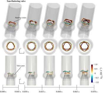


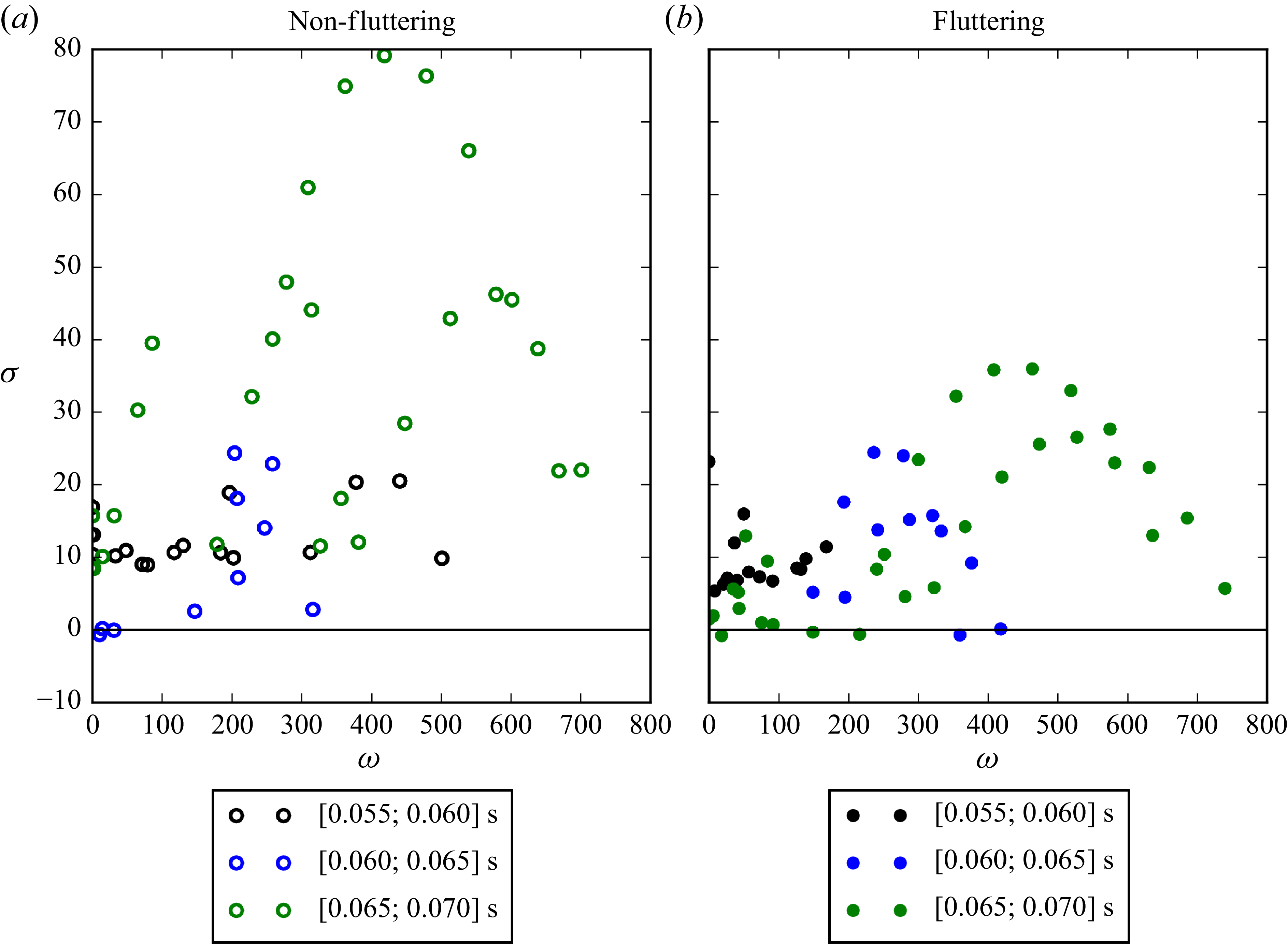


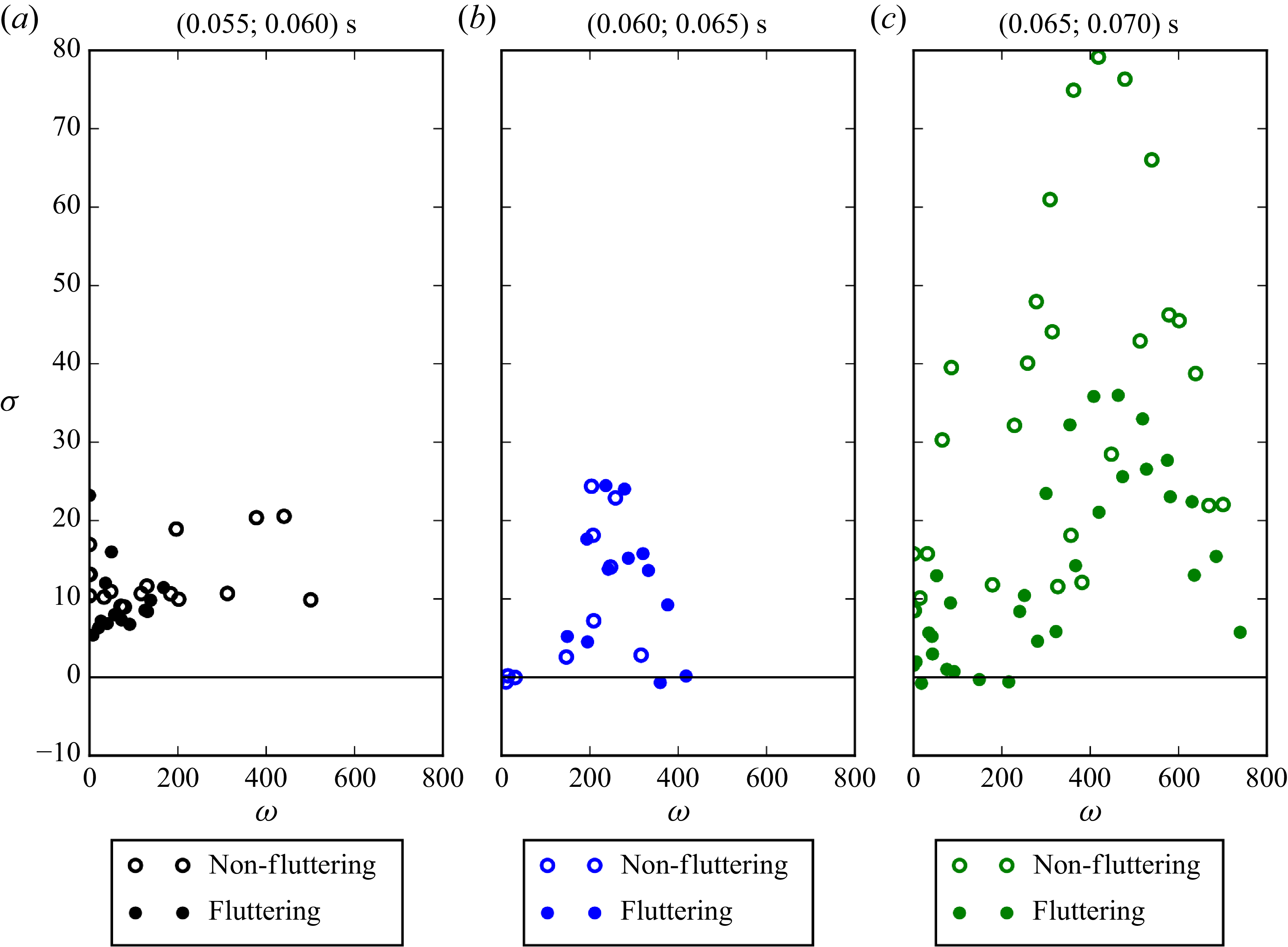


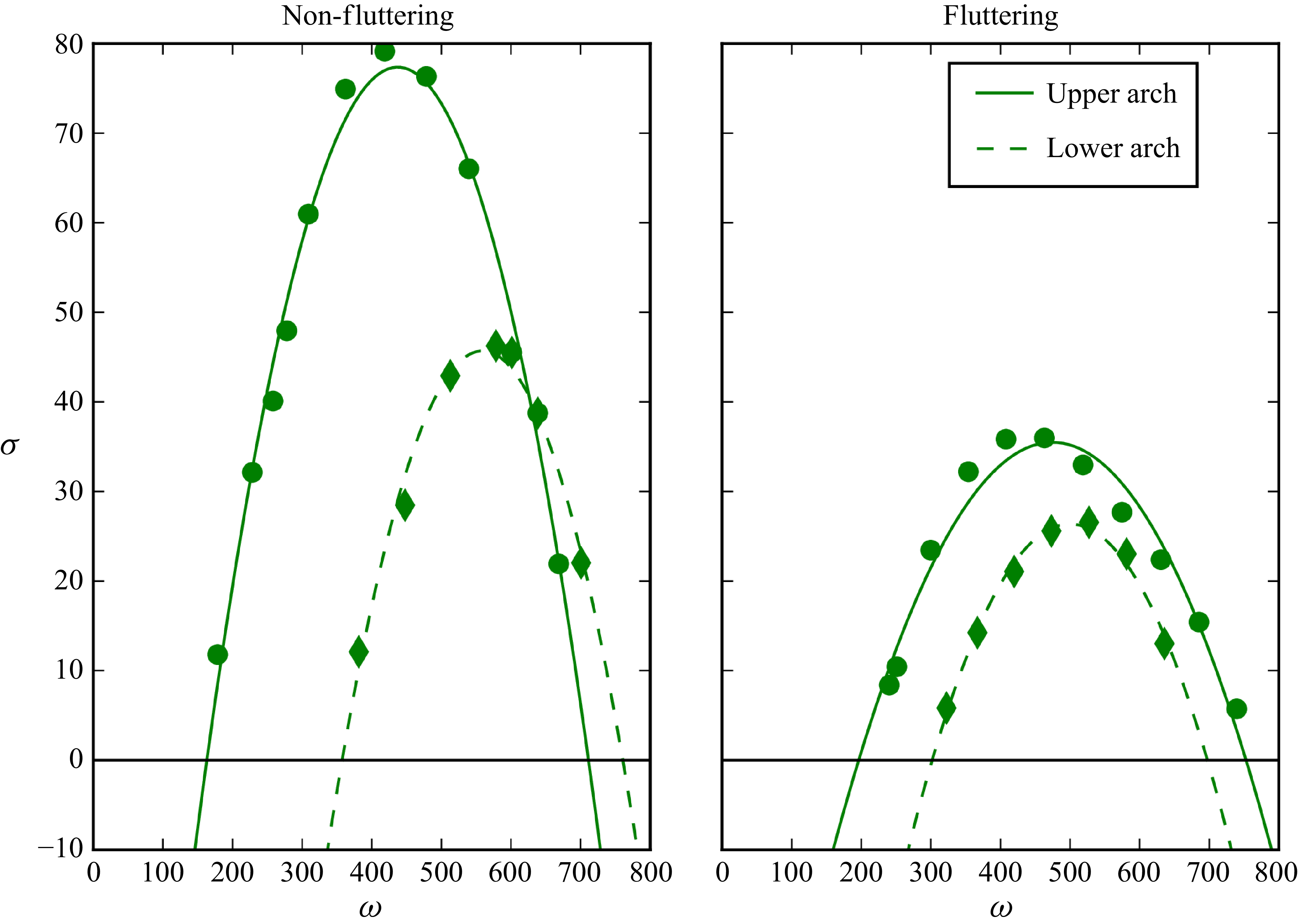


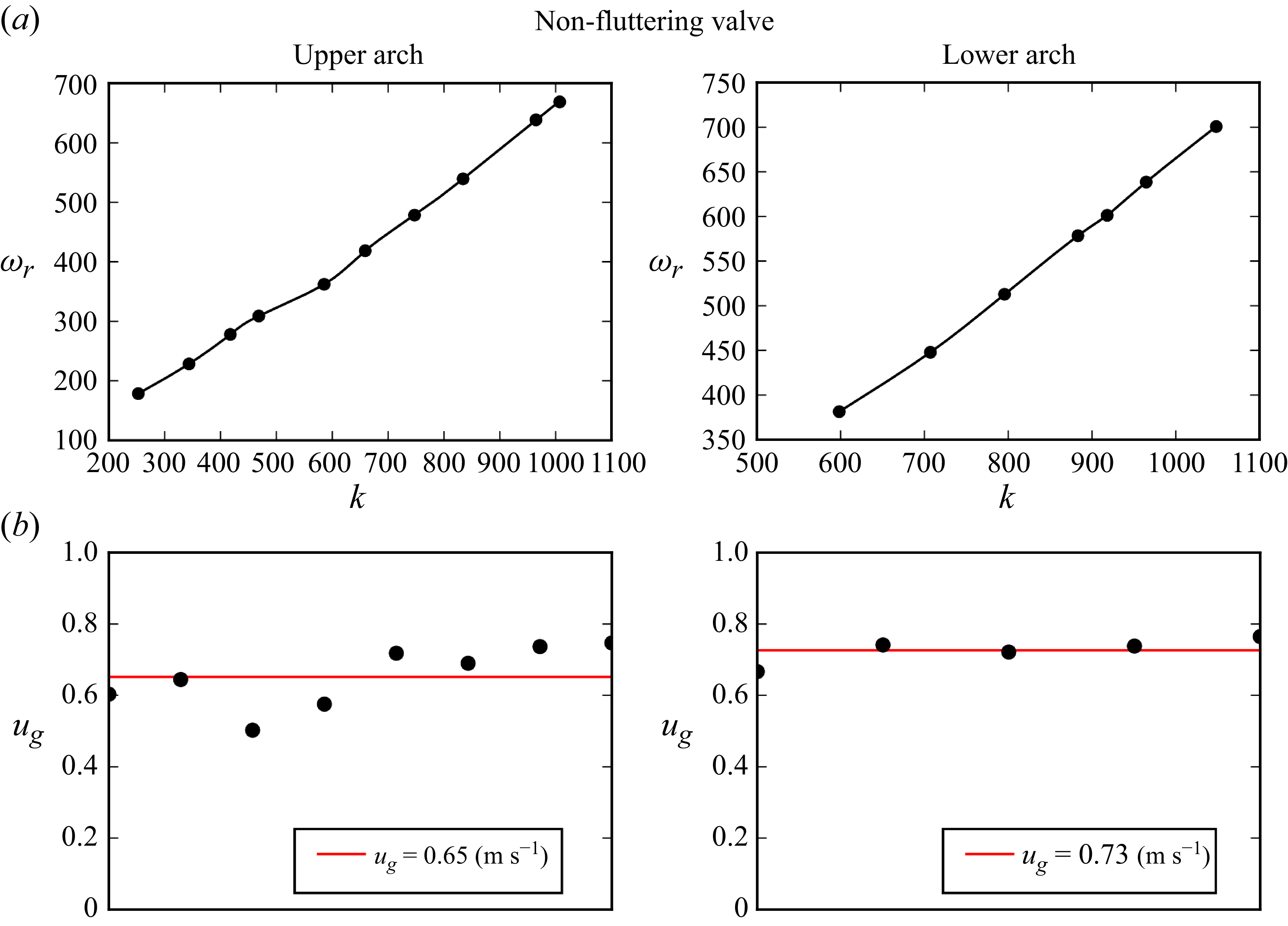


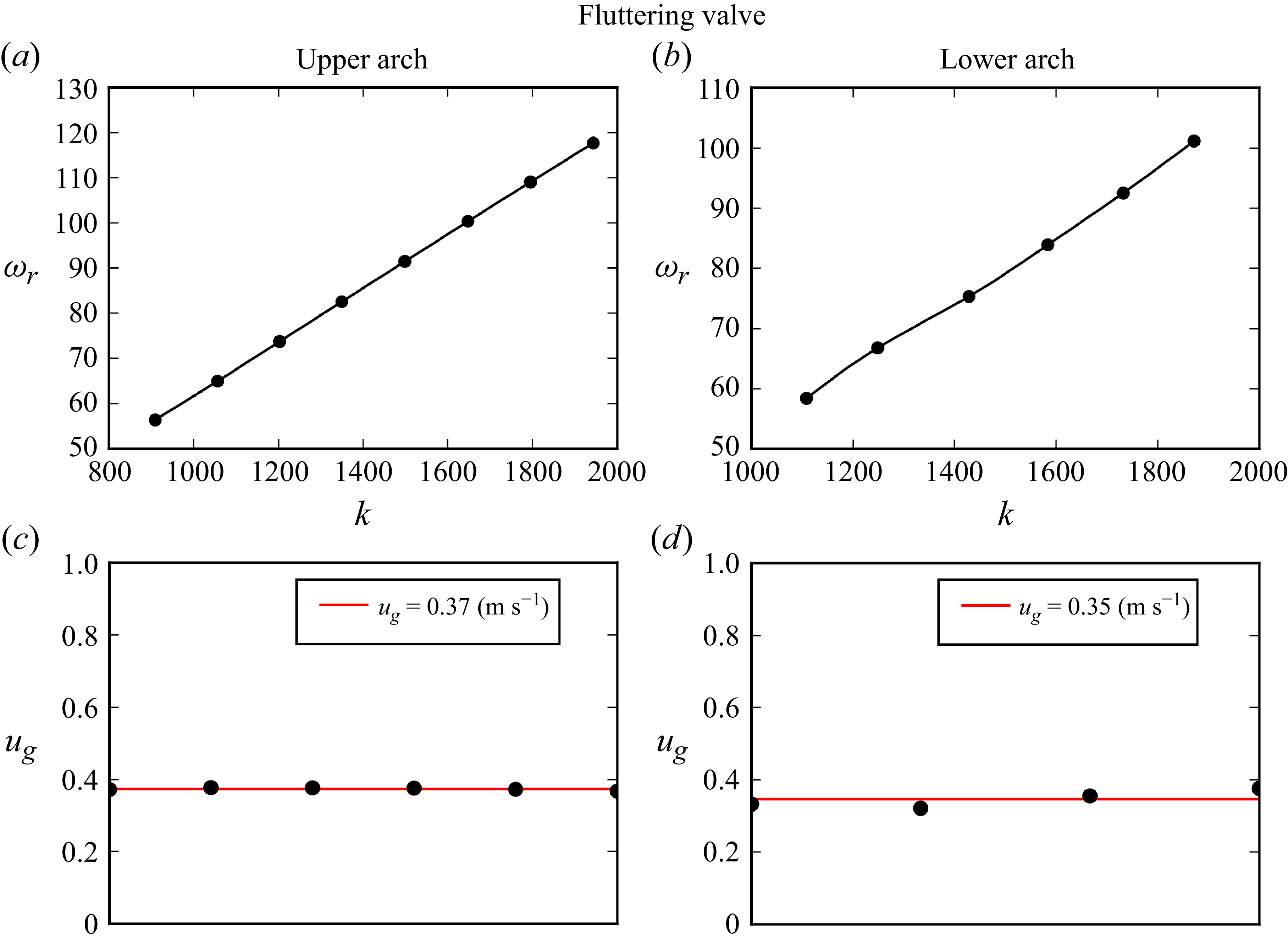


 Open access

